Embed Size (px)
Citation preview
Eduardo Haddad Fernando Perobelli
Aula 11 – Introdução ao GEMPACK
Fipe - Fundação Instituto de Pesquisas Econômicas 2
The Impact Project started in 1975 as part of the Industries Assistance Commission (now Productivity Commission)
The aim of the Impact Project was to produce general tools of use to all economists. These include the ORANI model and GEMPACK software
GEMPACK development began in 1984.
The main developers of GEMPACK are Jill Harrison, Mark Horridge and Ken Pearson
Histórico
Fipe - Fundação Instituto de Pesquisas Econômicas 3
Introduction
How to carry out a simulation?
How to implement the SJ model in GEMPACK?
Outline
Fipe - Fundação Instituto de Pesquisas Econômicas 4
General purpose package for GE models, not model specific
Allows modelers to concentrate on the economics of their models instead of computing problems
Aims to make modelers more productive
Document models for others
GEMPACK software
Fipe - Fundação Instituto de Pesquisas Econômicas 5
GEMPACK is a suite of general-purpose economic modeling software especially suitable for general and partial equilibrium models.
It can handle a wide range of economic behavior and also contains powerful capabilities for solving intertemporal models
GEMPACK provides software for calculating accurate solutions of an economic model, starting from an algebraic representation of the equations of the model.
Overview of GEMPACK Software
Fipe - Fundação Instituto de Pesquisas Econômicas 6
GEMPACK provides:
a) a simple language in which to describe and document the equations of your economic model;
b) a program which converts the equations of your model to a form ready for running simulations with the model;
c) options for varying the choice of exogenous and endogenous variables and the variables shocked;
d) utility programs to assist in managing the database on which the model is based.
Overview of GEMPACK Software
Fipe - Fundação Instituto de Pesquisas Econômicas 7
The (main) GEMPACK programs:
WinGEM – windows interface to GEMPACK
ViewHAR – for looking in the data in a Header Array File
ViewSOL – for looking at Solutions files
RunGEM – for automating simulations with models
TABmate – text editor for developing TABLO Input files
Overview of GEMPACK Software
Fipe - Fundação Instituto de Pesquisas Econômicas 8
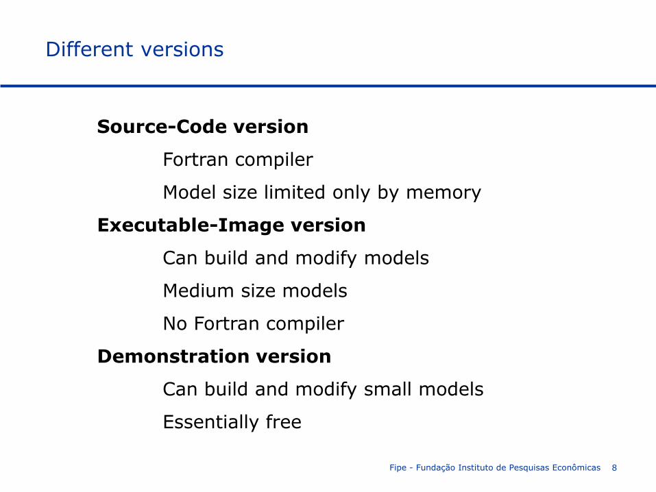
Source-Code version
Fortran compiler
Model size limited only by memory
Executable-Image version
Can build and modify models
Medium size models
No Fortran compiler
Demonstration version
Can build and modify small models
Essentially free
Different versions
Fipe - Fundação Instituto de Pesquisas Econômicas 9
Introduction
How to carry out a simulation?
How to implement the SJ model in GEMPACK?
Outline
Fipe - Fundação Instituto de Pesquisas Econômicas 10
In this part we will explain some of the terms used in GEMPACK;
Implementation
Simulation
Levels and percentage-change variables
Overview of GEMPACK Software
Fipe - Fundação Instituto de Pesquisas Econômicas 11
Write down equations in algebraic form
Collect data for initial solution
Construct TABLO Input file
Implementation
Fipe - Fundação Instituto de Pesquisas Econômicas 12
A model is implemented in GEMPACK when:
a) the equations describing its economic behavior are written down in an algebraic form following a syntax. (TABLO Input File)
b) data describing one solution of the model are assembled to be used as a starting point for simulations (ViewHAR)
Implementation
Fipe - Fundação Instituto de Pesquisas Econômicas 13
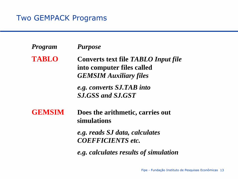
Two GEMPACK Programs
Program Purpose
TABLO Converts text file TABLO Input file
into computer files called
GEMSIM Auxiliary files
e.g. converts SJ.TAB into
SJ.GSS and SJ.GST
GEMSIM Does the arithmetic, carries out
simulations
e.g. reads SJ data, calculates
COEFFICIENTS etc.
e.g. calculates results of simulation
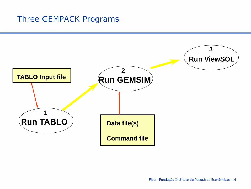
Three GEMPACK Programs
Fipe - Fundação Instituto de Pesquisas Econômicas 14
Run GEMSIM
Run TABLO
TABLO Input file
Data file(s)
Command file
1
2
Run ViewSOL
3

Fipe - Fundação Instituto de Pesquisas Econômicas 15
Many simulations are the answer to “WHAT IF” question such as:
“If the government were to increase tariffs by 10 percent, how much different would the economy be in 5 years time from what it would otherwise have been?”
Comparative-statics
Simulation
Fipe - Fundação Instituto de Pesquisas Econômicas 16
From the original solution supplied as the starting point, a simulation calculates a new solution to the equations of the model.
Within GEMPACK, the results of a simulation are usually reported as percentage changes from the original solution.
Solving models within GEMPACK is always done in the context of a simulation.
Simulation
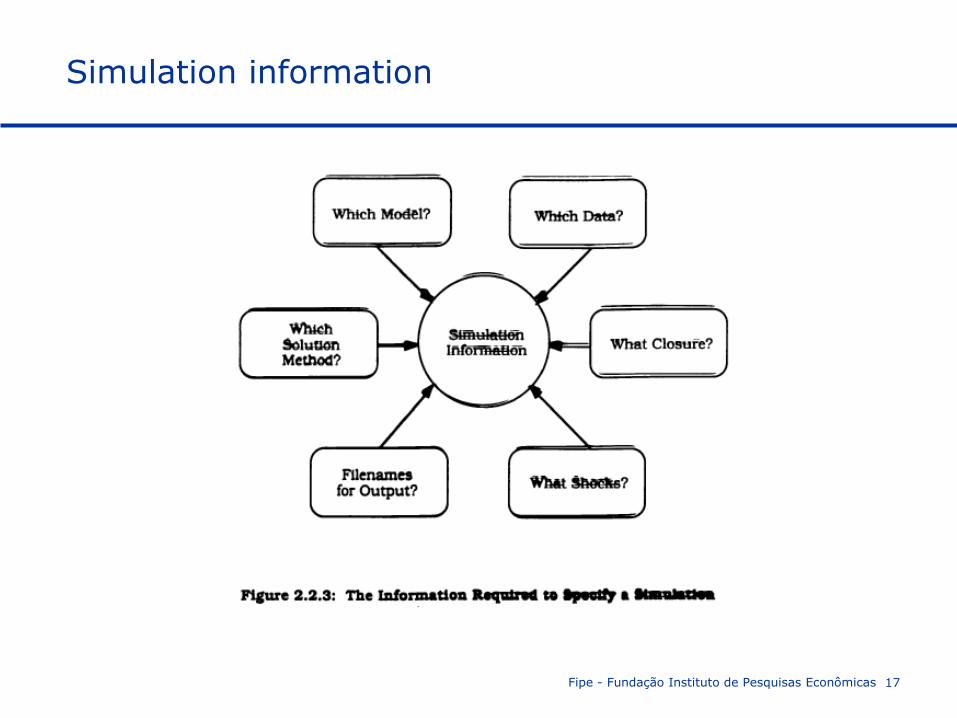
Simulation information
Fipe - Fundação Instituto de Pesquisas Econômicas 17

The GEMSIM method
Fipe - Fundação Instituto de Pesquisas Econômicas 18
Run GEMSIM
Run TABLO
TABLO
Input file
Data file(s)1
2
Command
file
Auxiliary files
ViewSOL
Solution file

TABLO-generated program
Fipe - Fundação Instituto de Pesquisas Econômicas 19
Run TABLO-
generated
program
Compile &
link
Run TABLO
TABLO Input file
Data file(s)
1
1b2
Command
file
Auxiliary files
ViewSOL
Solution file
Fipe - Fundação Instituto de Pesquisas Econômicas 20
There is a specification of the values of certain variables (“the exogenous ones” and the software calculates the values of the remaining variables (“the endogenous ones”).
The new values of the exogenous variables are usually given by specifying the percentage changes (increases or decreases) from their values in the original solution given as part of the implementation.
The process
Fipe - Fundação Instituto de Pesquisas Econômicas 21
When the model is implemented, the equations may be linearized (that is, differentiated).
The variables in these linearized equations are usually interpreted as percentage changes in the original variables.
The original variables (prices, quantities, etc.) are referred as the levels variables.
Levels and percentage-change variables
Fipe - Fundação Instituto de Pesquisas Econômicas 22
The (usually nonlinear) equations relating these levels variables are called the levels equations.
Levels equations:
D = PQ
The equation relates the dollar value, D, of a commodity to its price P ($ per ton) and its quantity Q (tons).
Levels and percentage-change variables
Fipe - Fundação Instituto de Pesquisas Econômicas 23
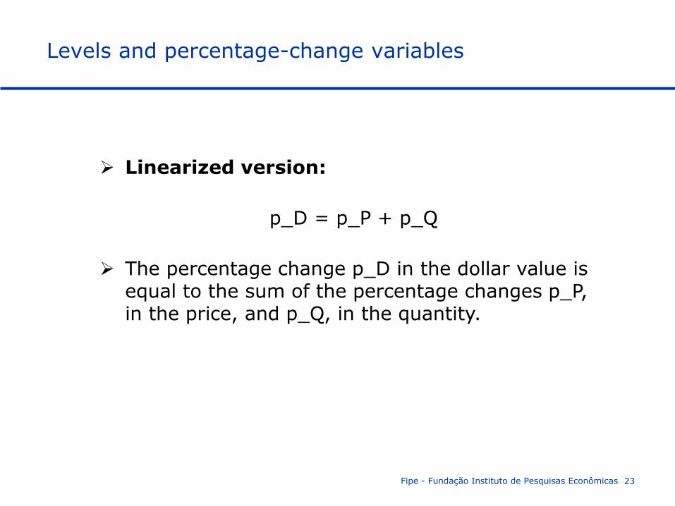
Linearized version:
p_D = p_P + p_Q
The percentage change p_D in the dollar value is equal to the sum of the percentage changes p_P, in the price, and p_Q, in the quantity.
Levels and percentage-change variables
Fipe - Fundação Instituto de Pesquisas Econômicas 24
The data for a model often consists of input-output data (giving dollar values) and parameters (including elasticities).
The data are usually sufficient to read off an initial solution to the levels equations (usually all basic prices are taken as 1 in the initial solution).
Data
Fipe - Fundação Instituto de Pesquisas Econômicas 25
Introduction
How to carry out a simulation?
How to implement the SJ model in GEMPACK?
Outline
Fipe - Fundação Instituto de Pesquisas Econômicas 26
Stylized Johansen described in Chapter 3 of Dixon et al (1992) and explained by Prof. Eduardo Haddad (Aula 8).
Single country
Two sectors “s1” and “s2” producing a single commodity (1, 2)
One household sector (0)
Two primary factors (3, 4)
Structure of the model
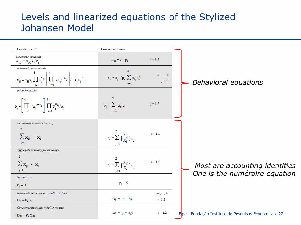
Levels and linearized equations of the Stylized Johansen Model
Fipe - Fundação Instituto de Pesquisas Econômicas 27
Behavioral equations
Most are accounting identities One is the numéraire equation
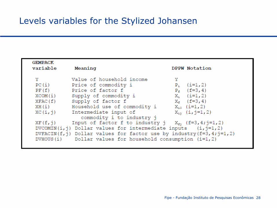
Levels variables for the Stylized Johansen
Fipe - Fundação Instituto de Pesquisas Econômicas 28
Fipe - Fundação Instituto de Pesquisas Econômicas 29
Most of variables have one or more arguments (indicating sectors and/or factors).
They are vector variables.
Variables which have no arguments (“Y” is the only one here) are referred to as scalar or macro variables.
Variables
Fipe - Fundação Instituto de Pesquisas Econômicas 30
PC(i) is regarded as a vector variable with 2 components, one for each sector, namely PC(“s1”) and PC(“s2”).
XF(f,j) is regarded as a vector variable with the following 4 components:
- component 1 XF (“labor”, “s1”): input of labor (factor 1) to sector 1.
- component 2 XF (“capital”, “s1”): input of capital (factor 2) to sector 1.
- component 3 XF (“labor”, “s2”): input of labor (factor 1) to sector 2
- component 4 XF (“capital”, “s2”): input of capital (factor 2) to sector 2.
Examples
Fipe - Fundação Instituto de Pesquisas Econômicas 31
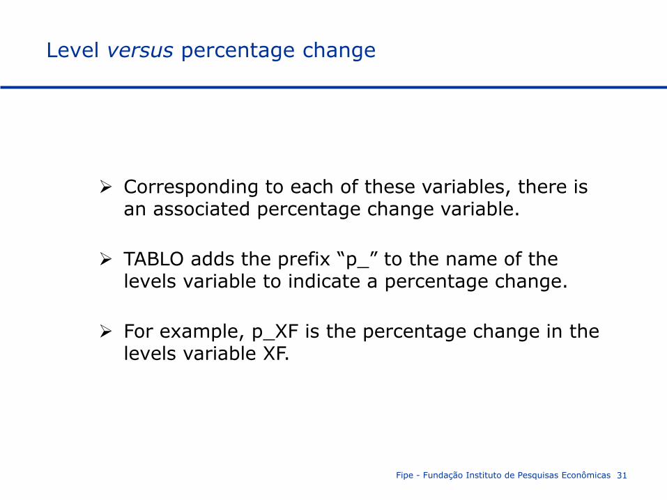
Corresponding to each of these variables, there is an associated percentage change variable.
TABLO adds the prefix “p_” to the name of the levels variable to indicate a percentage change.
For example, p_XF is the percentage change in the levels variable XF.
Level versus percentage change
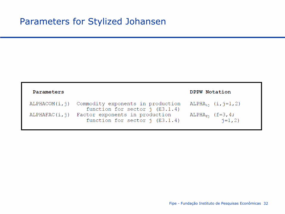
Parameters for Stylized Johansen
Fipe - Fundação Instituto de Pesquisas Econômicas 32
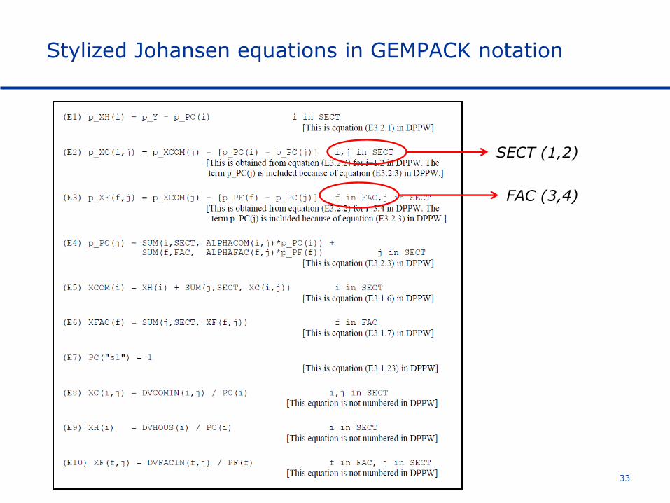
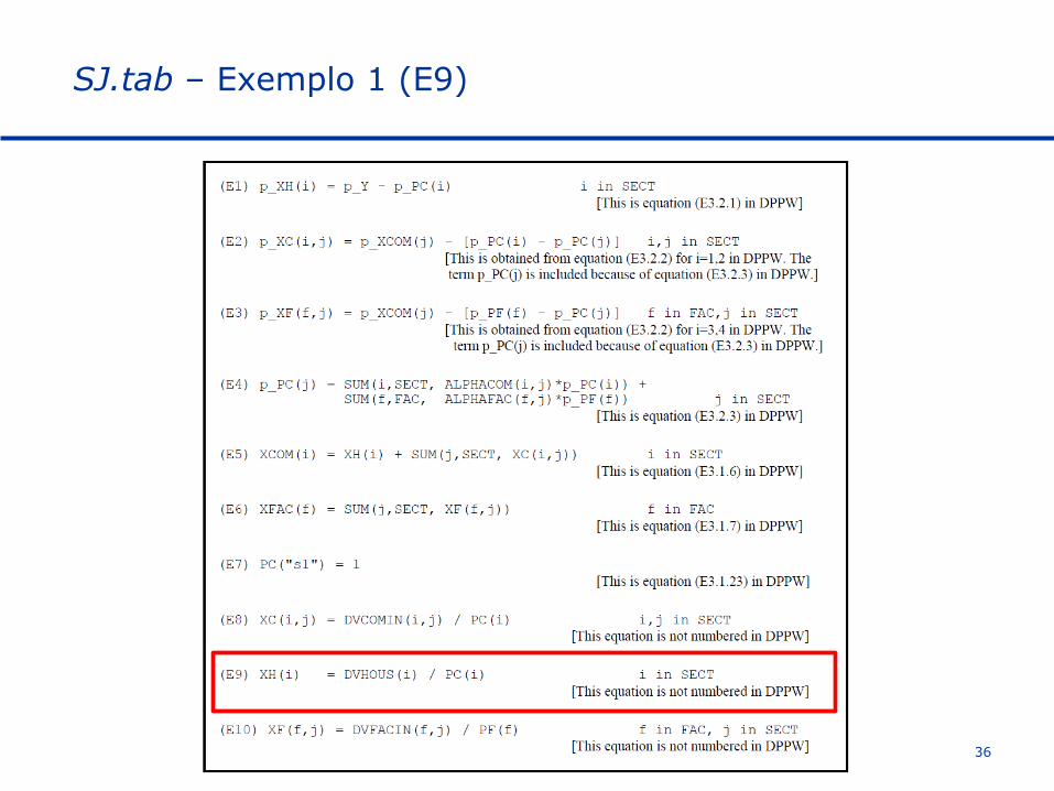
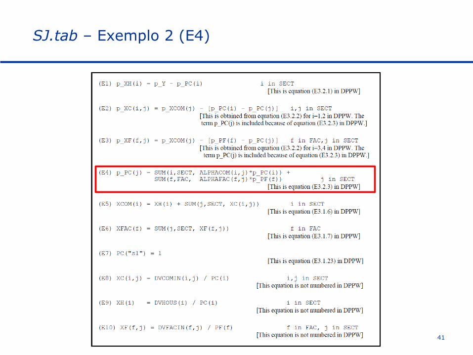
Stylized Johansen equations in GEMPACK notation
33
SECT (1,2)
FAC (3,4)
Fipe - Fundação Instituto de Pesquisas Econômicas 34
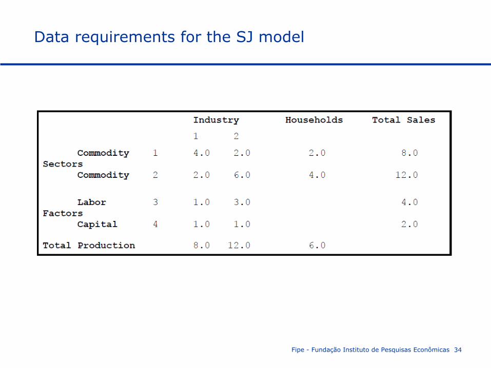
Data requirements for the SJ model
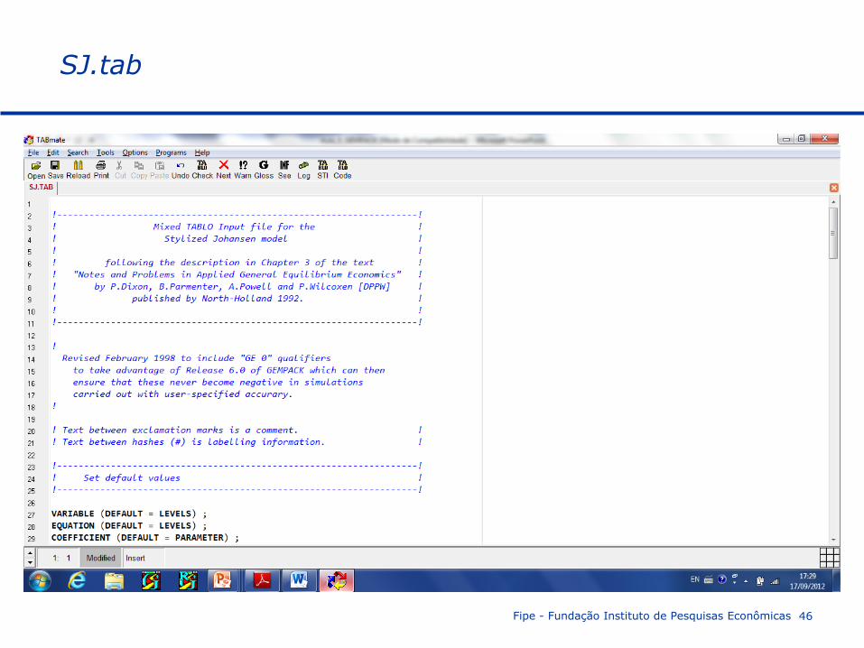
TABmate
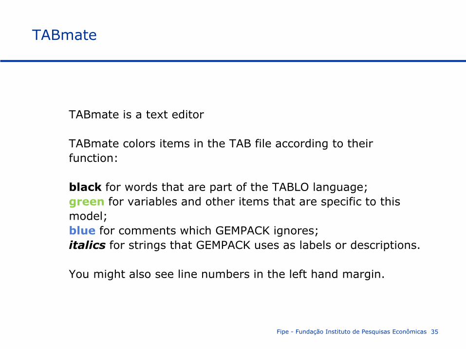
TABmate is a text editor
TABmate colors items in the TAB file according to their
function:
black for words that are part of the TABLO language;
green for variables and other items that are specific to this
model;
blue for comments which GEMPACK ignores;
italics for strings that GEMPACK uses as labels or descriptions.
You might also see line numbers in the left hand margin.
Fipe - Fundação Instituto de Pesquisas Econômicas 35
SJ.tab – Exemplo 1 (E9)
36
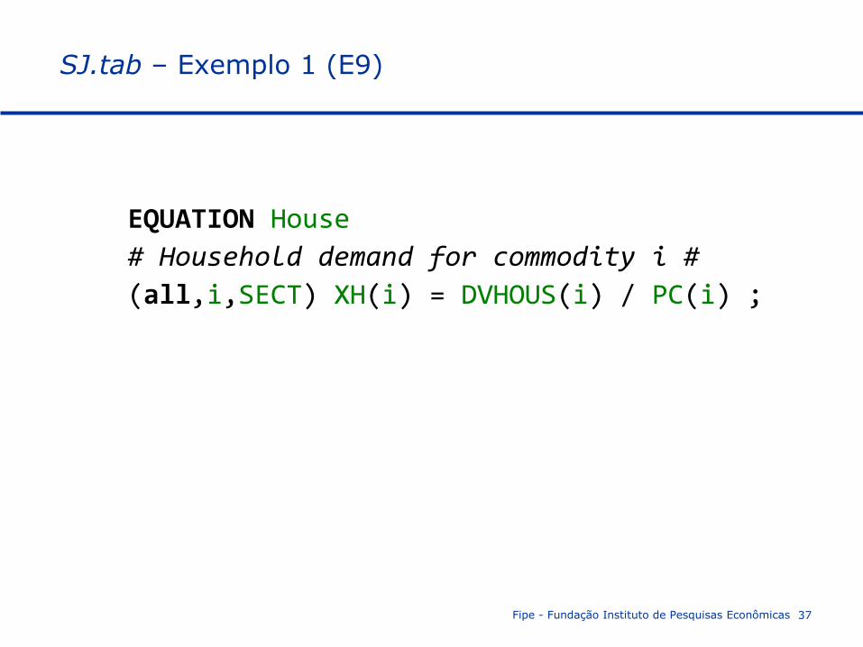
SJ.tab – Exemplo 1 (E9)
EQUATION House
# Household demand for commodity i #
(all,i,SECT) XH(i) = DVHOUS(i) / PC(i) ;
Fipe - Fundação Instituto de Pesquisas Econômicas 37
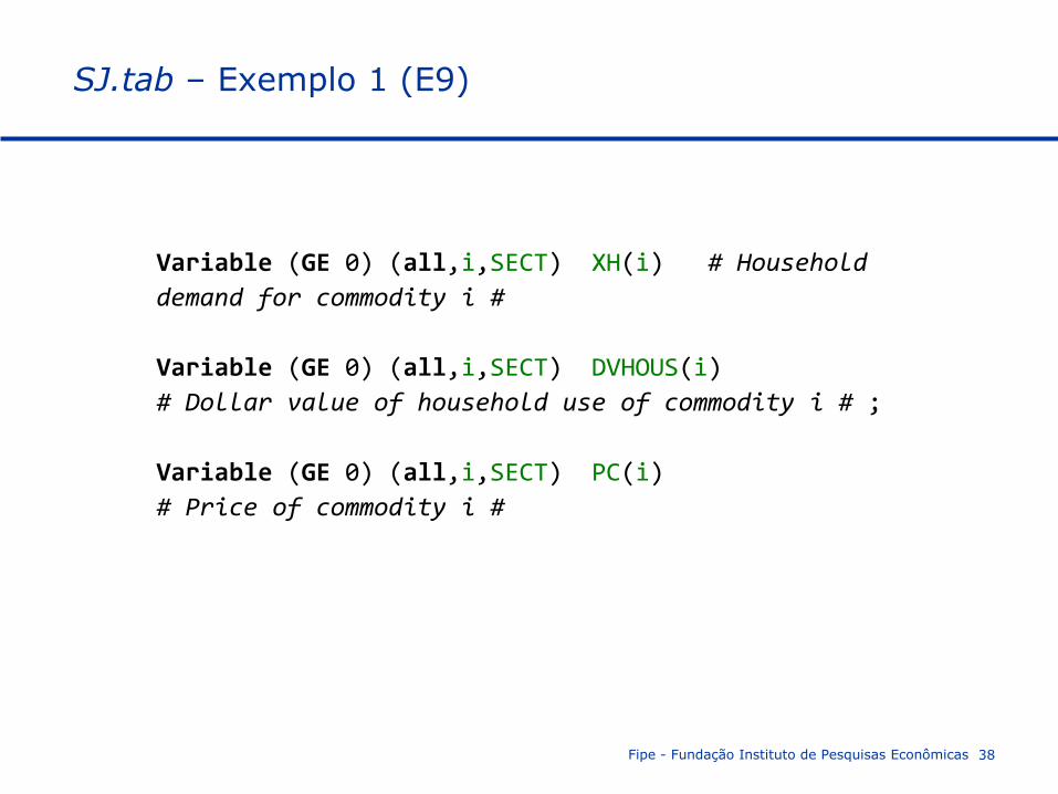
SJ.tab – Exemplo 1 (E9)
Variable (GE 0) (all,i,SECT) XH(i) # Household
demand for commodity i #
Variable (GE 0) (all,i,SECT) DVHOUS(i)
# Dollar value of household use of commodity i # ;
Variable (GE 0) (all,i,SECT) PC(i)
# Price of commodity i #
Fipe - Fundação Instituto de Pesquisas Econômicas 38
SJ.tab – Exemplo 1 (E9)
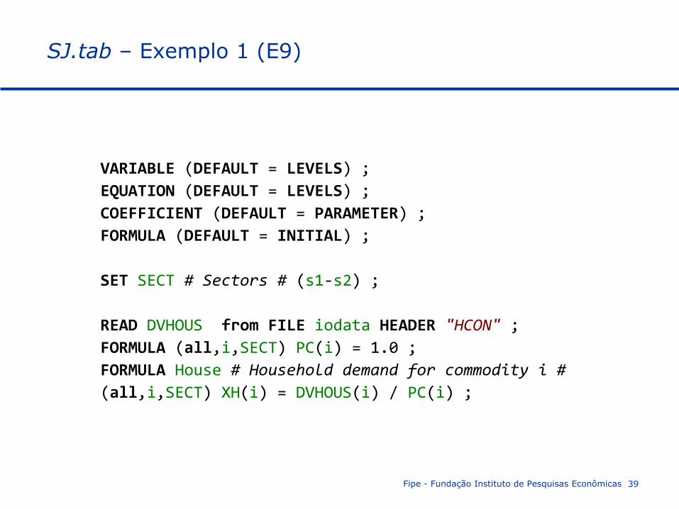
VARIABLE (DEFAULT = LEVELS) ;
EQUATION (DEFAULT = LEVELS) ;
COEFFICIENT (DEFAULT = PARAMETER) ;
FORMULA (DEFAULT = INITIAL) ;
SET SECT # Sectors # (s1-s2) ;
READ DVHOUS from FILE iodata HEADER "HCON" ;
FORMULA (all,i,SECT) PC(i) = 1.0 ;
FORMULA House # Household demand for commodity i #
(all,i,SECT) XH(i) = DVHOUS(i) / PC(i) ;
Fipe - Fundação Instituto de Pesquisas Econômicas 39
SJ.tab – Exemplo 1 (E9)
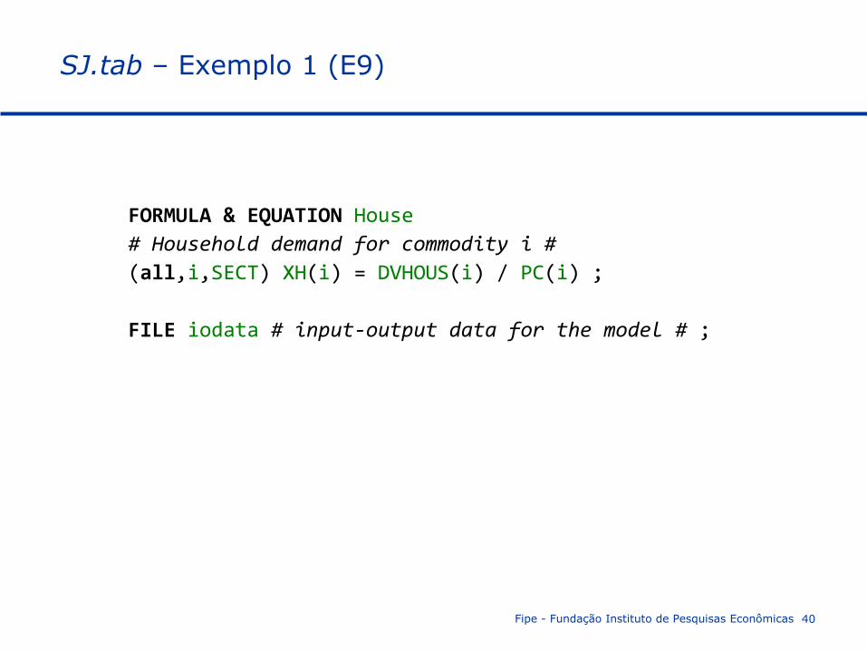
FORMULA & EQUATION House
# Household demand for commodity i #
(all,i,SECT) XH(i) = DVHOUS(i) / PC(i) ;
FILE iodata # input-output data for the model # ;
Fipe - Fundação Instituto de Pesquisas Econômicas 40
SJ.tab – Exemplo 2 (E4)
41
SJ.tab – Exemplo 2 (E4)
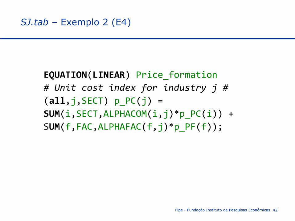
EQUATION(LINEAR) Price_formation
# Unit cost index for industry j #
(all,j,SECT) p_PC(j) =
SUM(i,SECT,ALPHACOM(i,j)*p_PC(i)) +
SUM(f,FAC,ALPHAFAC(f,j)*p_PF(f));
Fipe - Fundação Instituto de Pesquisas Econômicas 42
SJ.tab – Exemplo 2 (E4)
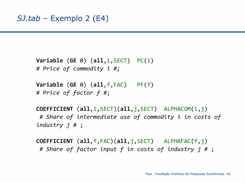
Variable (GE 0) (all,i,SECT) PC(i)
# Price of commodity i #;
Variable (GE 0) (all,f,FAC) PF(f)
# Price of factor f #;
COEFFICIENT (all,i,SECT)(all,j,SECT) ALPHACOM(i,j)
# Share of intermediate use of commodity i in costs of
industry j # ;
COEFFICIENT (all,f,FAC)(all,j,SECT) ALPHAFAC(f,j)
# Share of factor input f in costs of industry j # ;
Fipe - Fundação Instituto de Pesquisas Econômicas 43
SJ.tab – Exemplo 2 (E4)
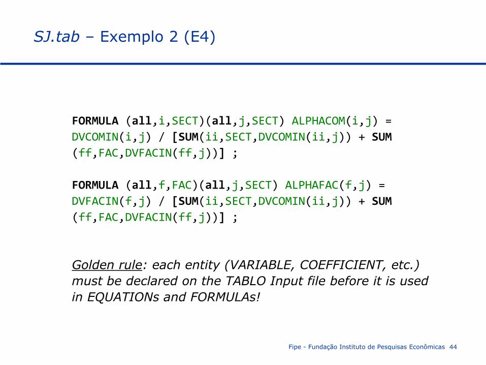
FORMULA (all,i,SECT)(all,j,SECT) ALPHACOM(i,j) =
DVCOMIN(i,j) / [SUM(ii,SECT,DVCOMIN(ii,j)) + SUM
(ff,FAC,DVFACIN(ff,j))] ;
FORMULA (all,f,FAC)(all,j,SECT) ALPHAFAC(f,j) =
DVFACIN(f,j) / [SUM(ii,SECT,DVCOMIN(ii,j)) + SUM
(ff,FAC,DVFACIN(ff,j))] ;
Golden rule: each entity (VARIABLE, COEFFICIENT, etc.)
must be declared on the TABLO Input file before it is used
in EQUATIONs and FORMULAs!
Fipe - Fundação Instituto de Pesquisas Econômicas 44
Fipe - Fundação Instituto de Pesquisas Econômicas 45
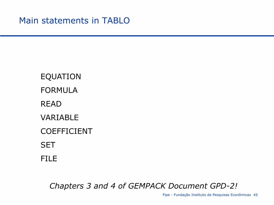
EQUATION
FORMULA
READ
VARIABLE
COEFFICIENT
SET
FILE
Chapters 3 and 4 of GEMPACK Document GPD-2!
Main statements in TABLO
SJ.tab
Fipe - Fundação Instituto de Pesquisas Econômicas 46
Fipe - Fundação Instituto de Pesquisas Econômicas 47
1. Starting WinGEM
2. Preparing a directory for Model SJ
3. Setting the working directory
4. Editing text files in WinGEM
5. Looking at the data directly (VIEWHAR)
6. Simulations with the SJ model
Examples
Fipe - Fundação Instituto de Pesquisas Econômicas 48
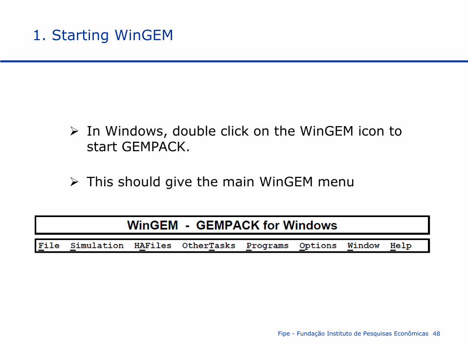
In Windows, double click on the WinGEM icon to start GEMPACK.
This should give the main WinGEM menu
1. Starting WinGEM
Fipe - Fundação Instituto de Pesquisas Econômicas 49
To keep all example files for the SJ model together in one area, we should create a separate directory \SJ for these files and how to copy the relevant files into this directory.
2. Preparing a directory for Model SJ
3. Setting the working directory
Choose a working directory (for SJ model the working
directory needs to be the directory \SJ you have just
created)
To set this, first click on File in the main WinGEM menu
In the drop-down menu, click on the menu item
Change both default directories…
So the sequence of clicks (first File then Change both
default directories) is
File|Change both default directories…
Fipe - Fundação Instituto de Pesquisas Econômicas 50
5. Looking at the data directly (VIEWHAR)
The input-output data used in SJ model are contained in
the data file SJ.DAT
This is a special GEMPACK binary file – called Header
Array file
Thus to look at SJ.DAT you have to use a special program
to read Header Array files, called ViewHAR
HA Files| View VIEWHAR
The viewHAR window will appear
Click on File|Open… and selected the file SJ.DAT
This will open the file SJ.DAT and show the contents on the
screen
Fipe - Fundação Instituto de Pesquisas Econômicas 51
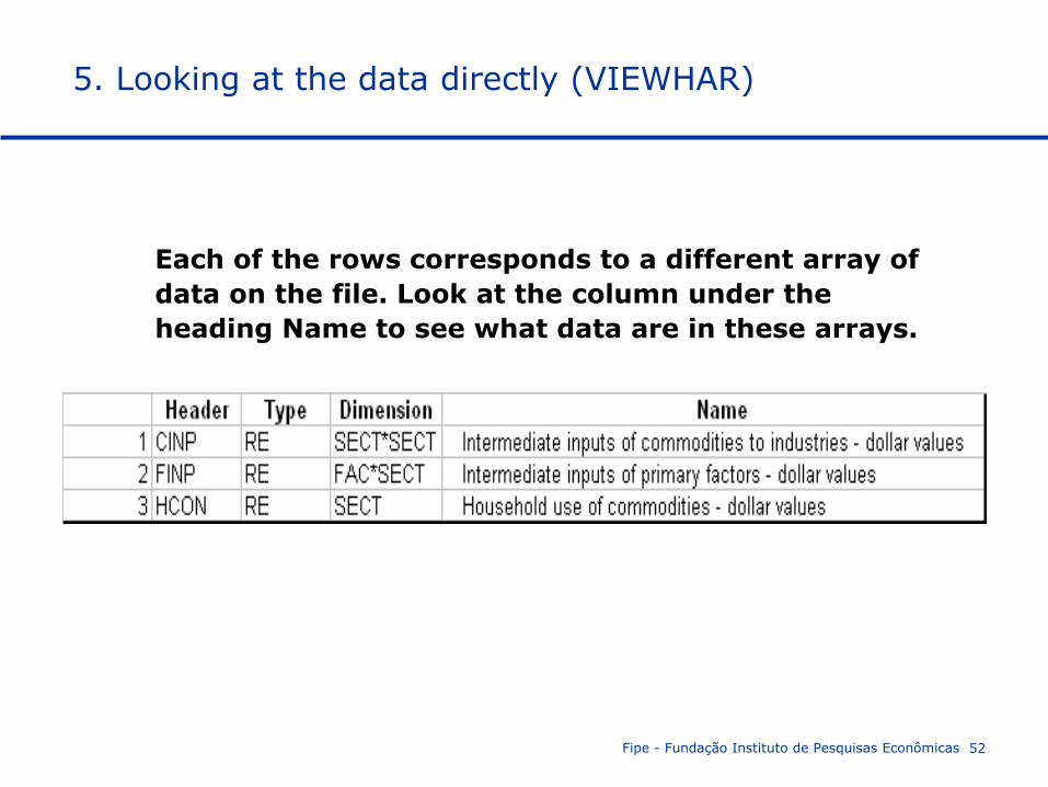
5. Looking at the data directly (VIEWHAR)
Each of the rows corresponds to a different array of
data on the file. Look at the column under the
heading Name to see what data are in these arrays.
Fipe - Fundação Instituto de Pesquisas Econômicas 52
5. Looking at the data directly (VIEWHAR)
The first array is the “Intermediate inputs of commodities
to industries – dollar values”
The Header CINP is just a label for this array (headers can
have up to 4 characters).
The array is of Type RE. The R means this is an array of
real numbers. The E means that this array has set and
element labeling.
Double click on CINP to see the numbers in this array.
Fipe - Fundação Instituto de Pesquisas Econômicas 53
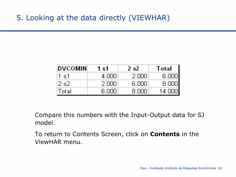
5. Looking at the data directly (VIEWHAR)
Compare this numbers with the Input-Output data for SJ
model.
To return to Contents Screen, click on Contents in the
ViewHAR menu.
Fipe - Fundação Instituto de Pesquisas Econômicas 54
Fipe - Fundação Instituto de Pesquisas Econômicas 55
We have to choose a closure:
- Supply of the two factors, labor and capital, are the exogenous variables
Thus we will specify the percentage changes in the variable XFAC, namely p_XFAC, and solve the model to find the percentage changes in all the other variables.
6. Simulations with the SJ model
Fipe - Fundação Instituto de Pesquisas Econômicas 56
For this simulation, we increase the supply of labor by 10 per cent and hold the supply of capital fixed
The starting point for any simulations with Stylized Johansen model are:
- the TABLO Input file (called SJ. TAB) and
- the data file (called SJ.DAT)
6. Simulations with the SJ model
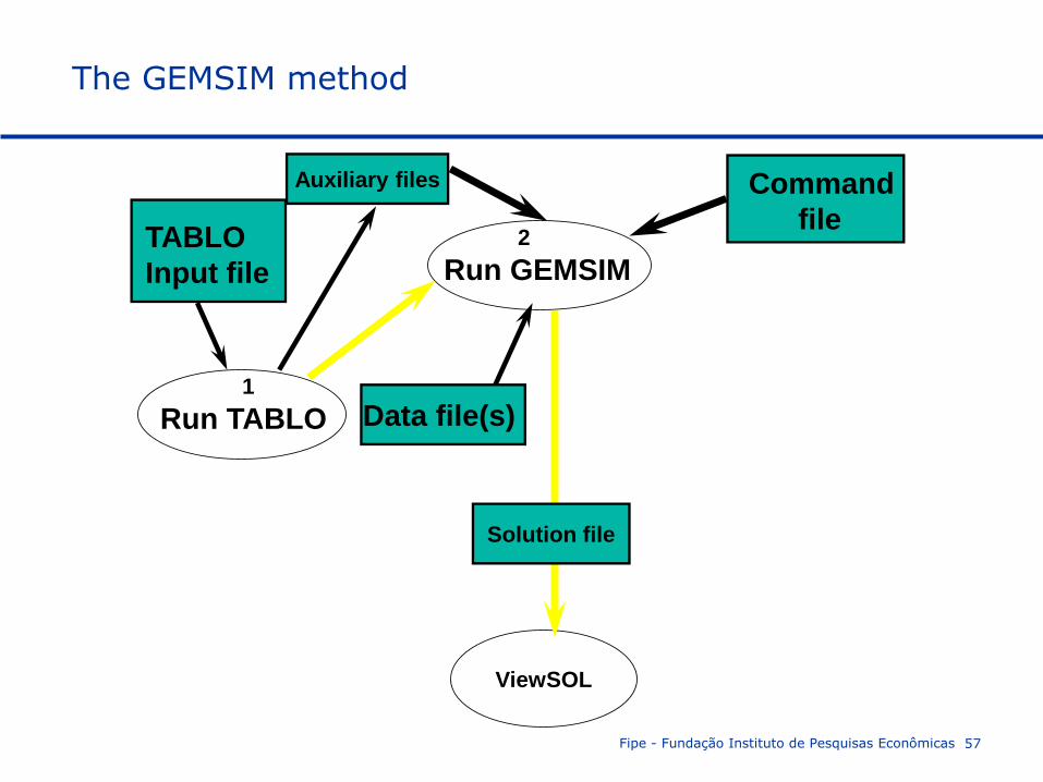
The GEMSIM method
Fipe - Fundação Instituto de Pesquisas Econômicas 57
Run GEMSIM
Run TABLO
TABLO
Input file
Data file(s)1
2
Command
file
Auxiliary files
ViewSOL
Solution file
Fipe - Fundação Instituto de Pesquisas Econômicas 58
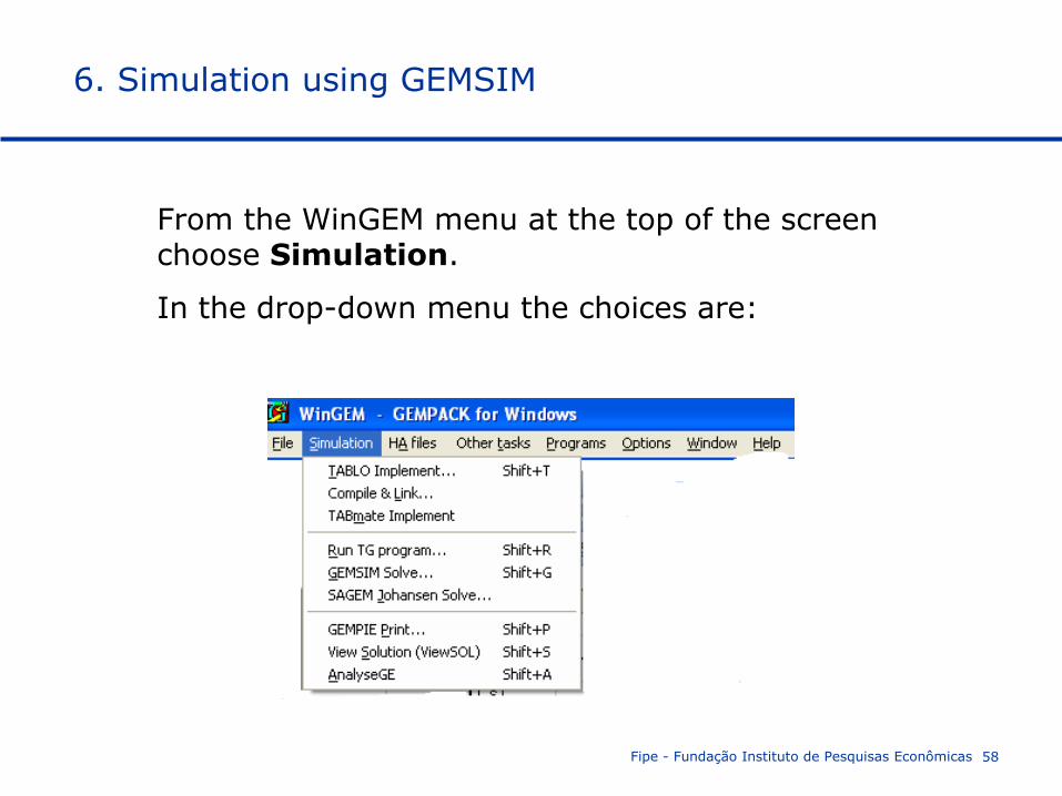
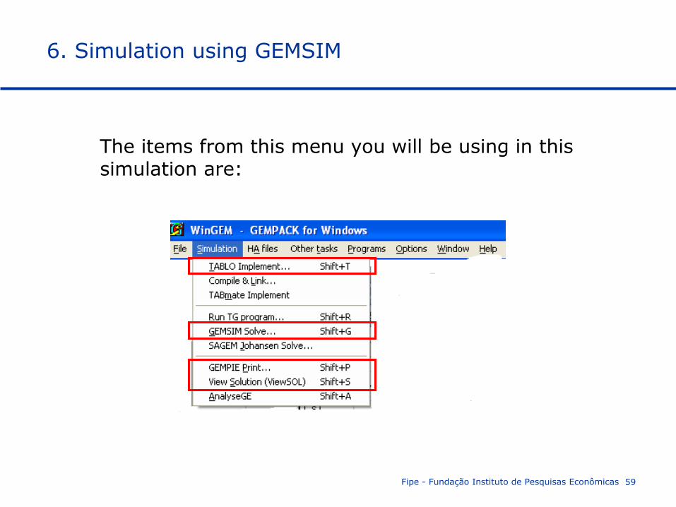
From the WinGEM menu at the top of the screen choose Simulation.
In the drop-down menu the choices are:
6. Simulation using GEMSIM
Fipe - Fundação Instituto de Pesquisas Econômicas 59
The items from this menu you will be using in this simulation are:
6. Simulation using GEMSIM
Fipe - Fundação Instituto de Pesquisas Econômicas 60
There are three steps involved in carrying out a simulation using GEMPACK:
STEP 1 – Implement the model (TABLO)
STEP 2 – Solve the equations of the model (GEMSIM)
STEP 3 – View the results (GEMPIE and VIEWSOL)
WinGEM will guide you through these steps and indicate what to do next.
6. Simulation using GEMSIM
Fipe - Fundação Instituto de Pesquisas Econômicas 61
Step 1:
Simulation / TABLO Implement…
TABLO Options… (PGS)
Go to GEMSIM
Step 2:
File SJLB.CMF
6. Simulation using GEMSIM
Fipe - Fundação Instituto de Pesquisas Econômicas 62
Step 3:
GEMPIE versus VIEWSOL
The updated data – another result of the simulation
File SJLB.UPD
6. Simulation using GEMSIM
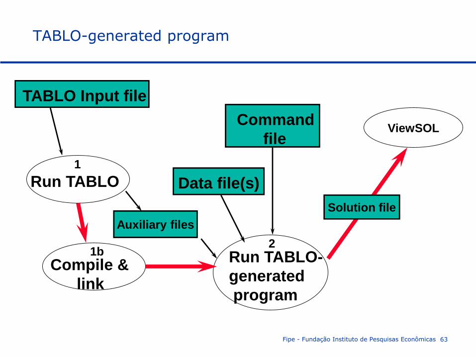
TABLO-generated program
Fipe - Fundação Instituto de Pesquisas Econômicas 63
Run TABLO-
generated
program
Compile &
link
Run TABLO
TABLO Input file
Data file(s)
1
1b2
Command
file
Auxiliary files
ViewSOL
Solution file

Fipe - Fundação Instituto de Pesquisas Econômicas 64
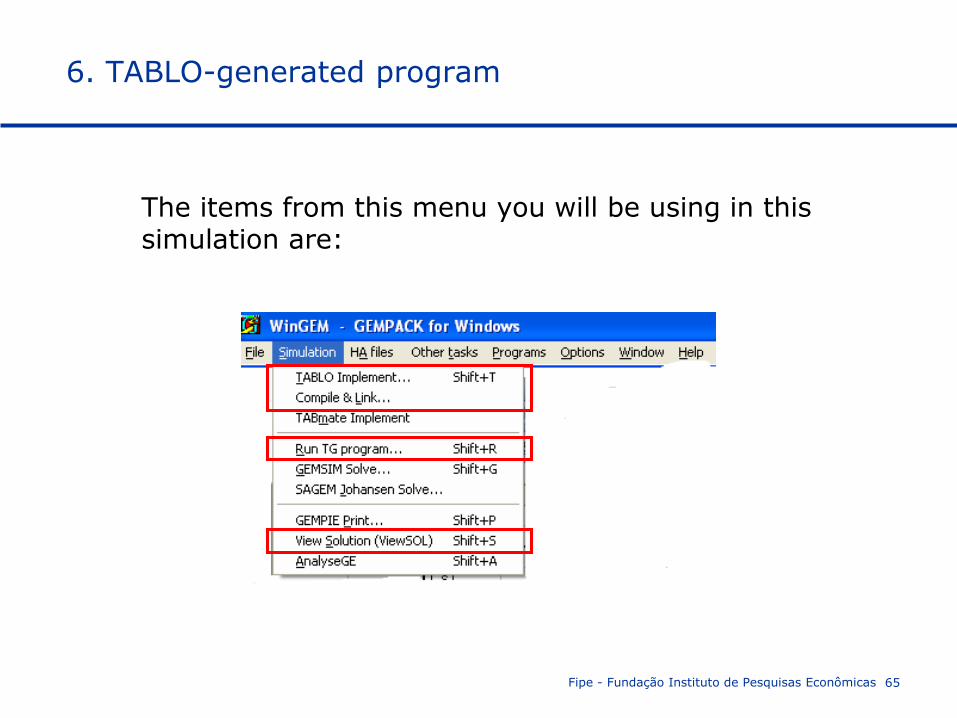
From the WinGEM menu at the top of the screen choose Simulation.
In the drop-down menu the choices are:
6. TABLO-generated program
Fipe - Fundação Instituto de Pesquisas Econômicas 65
The items from this menu you will be using in this simulation are:
6. TABLO-generated program
Fipe - Fundação Instituto de Pesquisas Econômicas 66
In the TABLO-generated program method, the GEMPACK program TABLO is used to convert the algebraic equations of the economic model into a Fortran program specific to your model.
This Fortran program (which is referred to as the TABLO-generated program or TG Program in the menu) is compiled and linked to a library of GEMPACK subroutines.
The executable image of the TABLO-generated program produced by the compiler is used to run simulations on the model.
6. TABLO-generated program
Fipe - Fundação Instituto de Pesquisas Econômicas 67
There are three steps involved in carrying out a simulation using GEMPACK:
STEP 1 – Implement the model
STEP 2 – Solve the equations of the model
STEP 3 – View the results
WinGEM and RunGEM will guide you through these steps and indicate what to do next.
6. TABLO-generated program
Fipe - Fundação Instituto de Pesquisas Econômicas 68
STEP 1 – Implement the model SJ using TABLO
Step 1 (a) – Run TABLO to create the TABLO-generated program
The TABLO Input file is called SJ.TAB. It contains the theory of the SJ model.
Choose:
Simulation|TABLO Implement….
6. TABLO-generated program
Fipe - Fundação Instituto de Pesquisas Econômicas 69
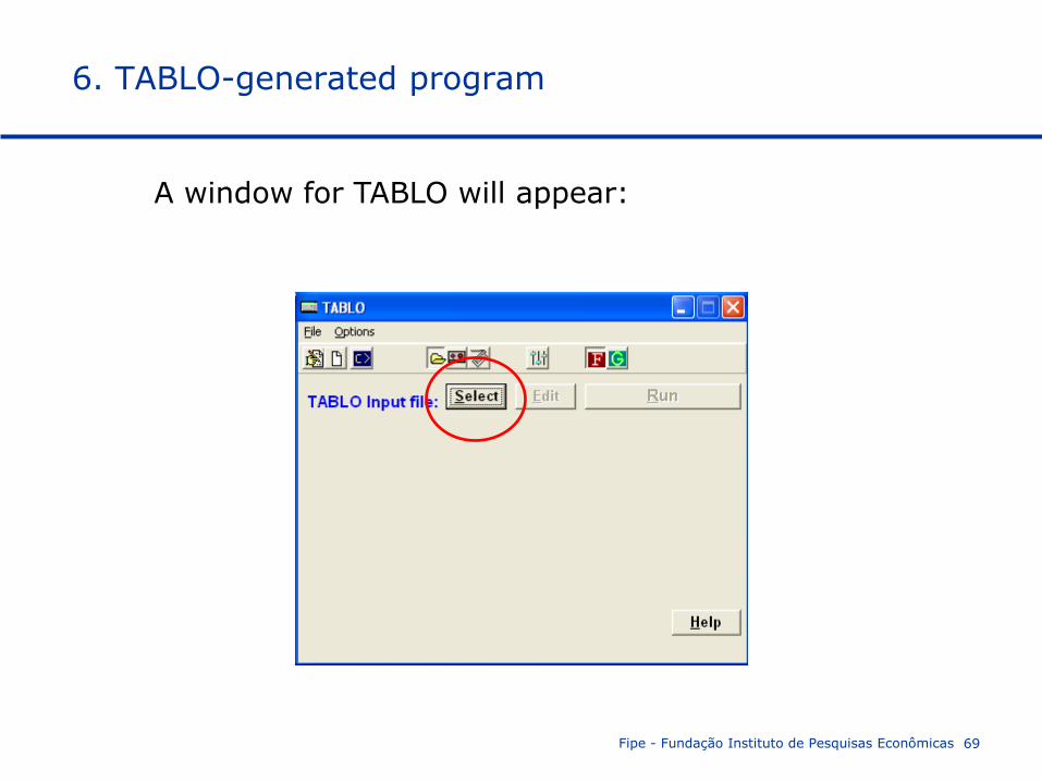
A window for TABLO will appear:
6. TABLO-generated program
Fipe - Fundação Instituto de Pesquisas Econômicas 70
Click on the Select button to select the name of the TABLO Input file SJ.TAB. This is all TABLO need to implement a model.
In the menu for the TABLO window, select Options menu item. Then in this menu choose
TABLO Options…..
A new TABLO Options window will appear…
6. TABLO-generated program
Fipe - Fundação Instituto de Pesquisas Econômicas 71
6. TABLO-generated program
Fipe - Fundação Instituto de Pesquisas Econômicas 72
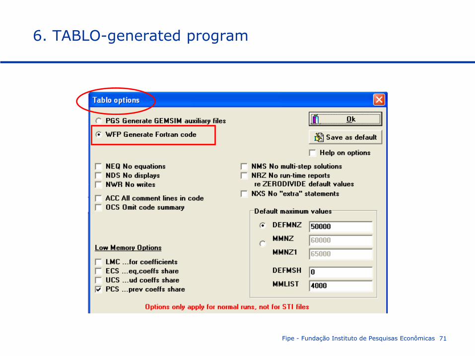
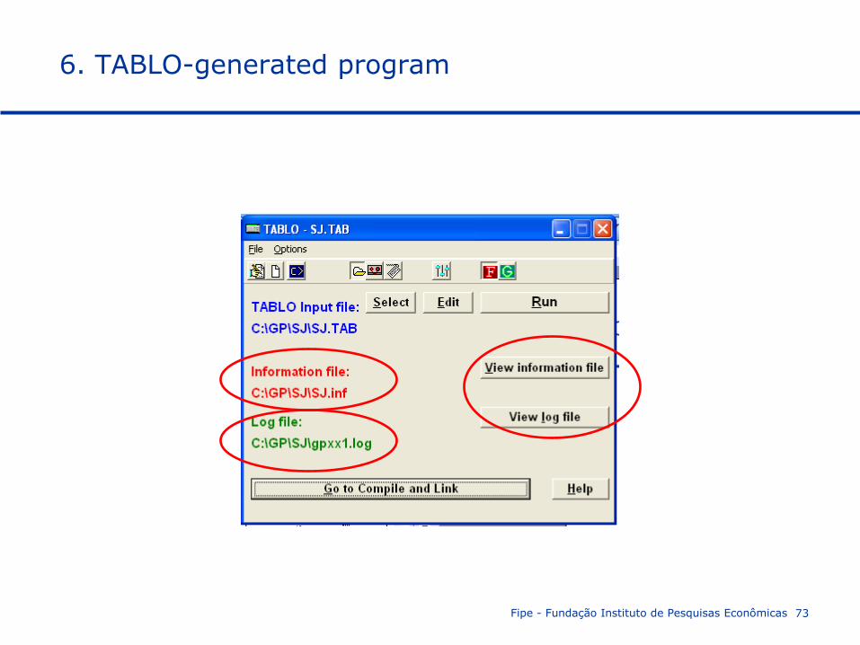
We will choose the option WFP because we want you to create the TABLO-generated program.
Then click on Ok button to return to the TABLO window.
Click on Run button
The program runs TABLO in a DOS box and when complete, returns to the TABLO window with the names of files it has created: the information file SJ.INF and Log file.
To look at files click on View buttons beside them.
6. TABLO-generated program
Fipe - Fundação Instituto de Pesquisas Econômicas 73
6. TABLO-generated program
Fipe - Fundação Instituto de Pesquisas Econômicas 74
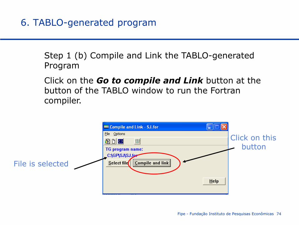
Step 1 (b) Compile and Link the TABLO-generated Program
Click on the Go to compile and Link button at the button of the TABLO window to run the Fortran compiler.
6. TABLO-generated program
File is selected
Click on this button
Fipe - Fundação Instituto de Pesquisas Econômicas 75
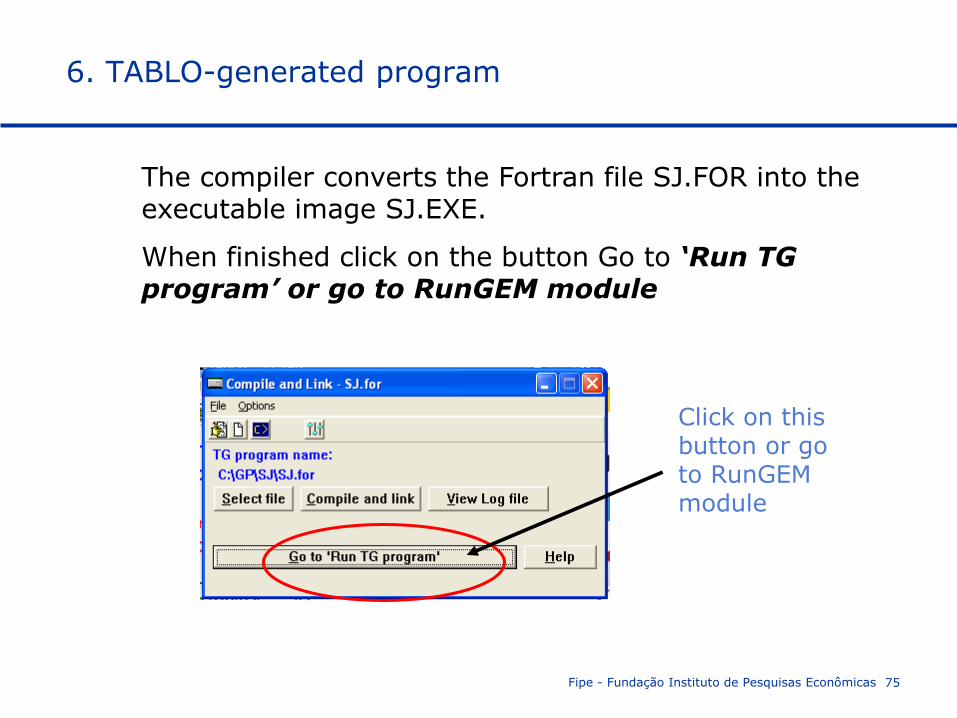
The compiler converts the Fortran file SJ.FOR into the executable image SJ.EXE.
When finished click on the button Go to ‘Run TG program’ or go to RunGEM module
6. TABLO-generated program
Click on this button or go to RunGEM module
Fipe - Fundação Instituto de Pesquisas Econômicas 76
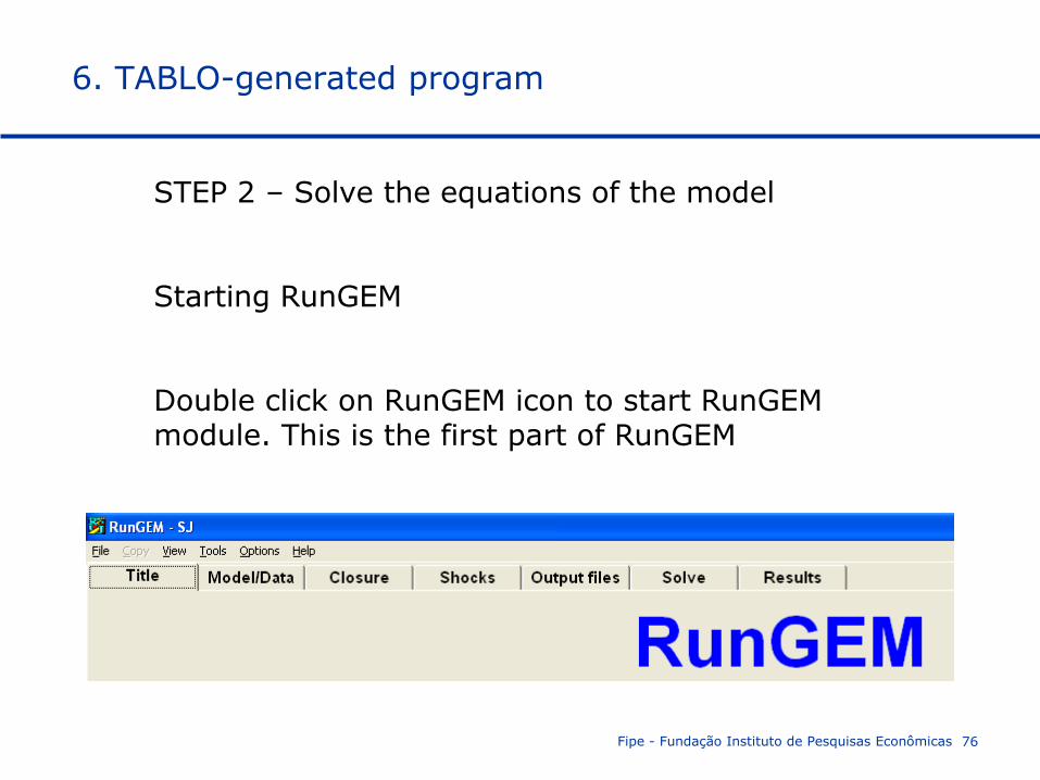
STEP 2 – Solve the equations of the model
Starting RunGEM
Double click on RunGEM icon to start RunGEM module. This is the first part of RunGEM
6. TABLO-generated program
Fipe - Fundação Instituto de Pesquisas Econômicas 77
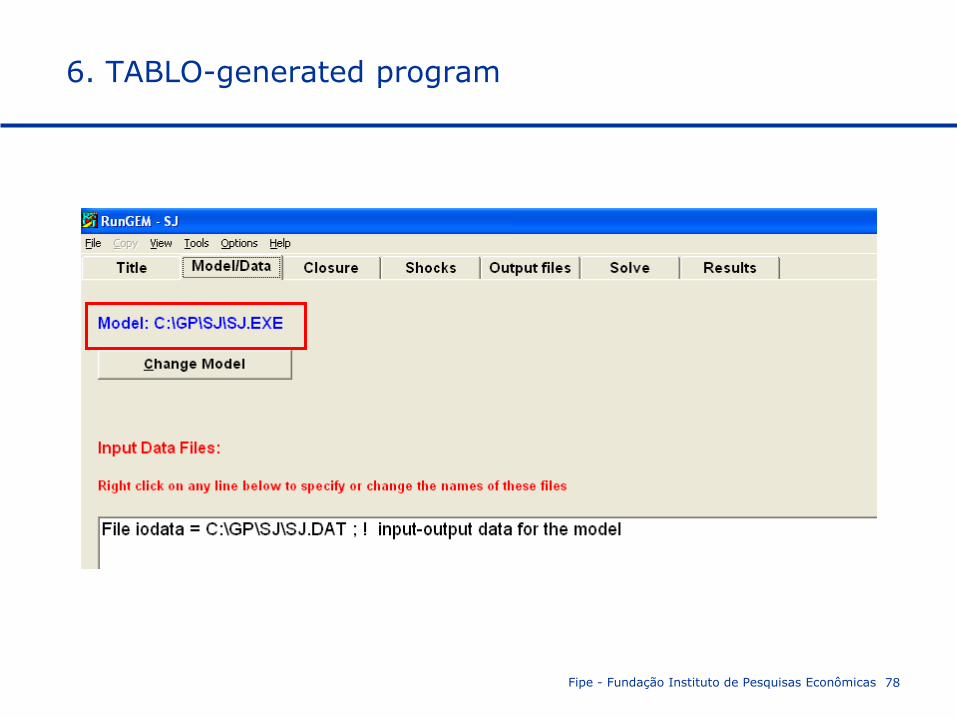
To change from Title to Model/Data for exemple is only necessary to click on the names.
Select the Model:
Go to Model/Data page by clicking on its tab.
Click on button Change Model do select your model.
Select the file SJ.EXE.
6. TABLO-generated program
Fipe - Fundação Instituto de Pesquisas Econômicas 78
6. TABLO-generated program
Fipe - Fundação Instituto de Pesquisas Econômicas 79
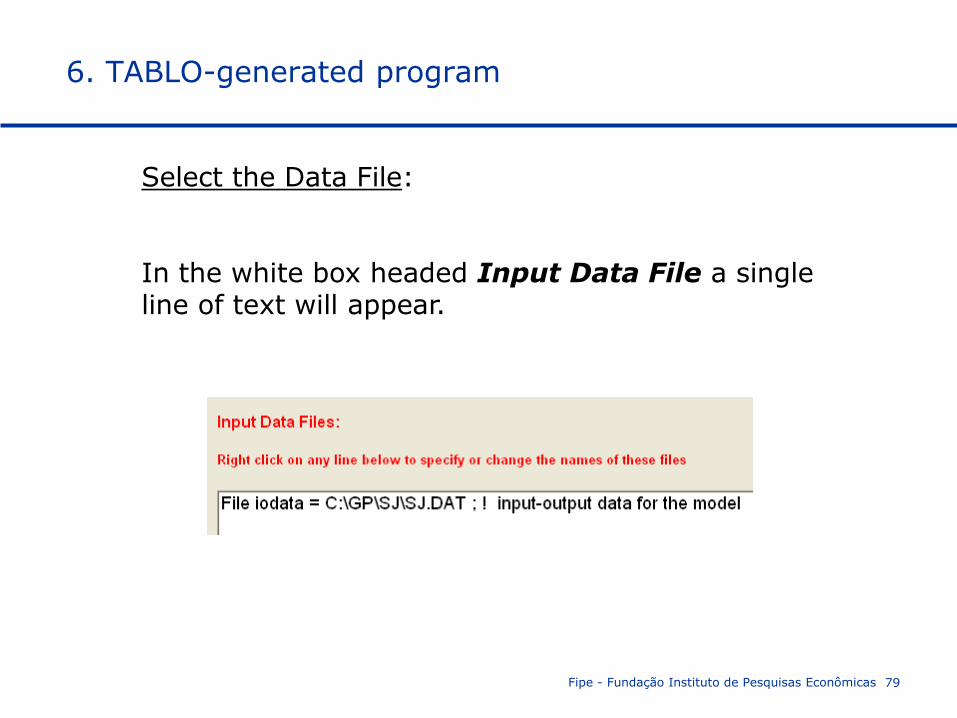
Select the Data File:
In the white box headed Input Data File a single line of text will appear.
6. TABLO-generated program
Fipe - Fundação Instituto de Pesquisas Econômicas 80
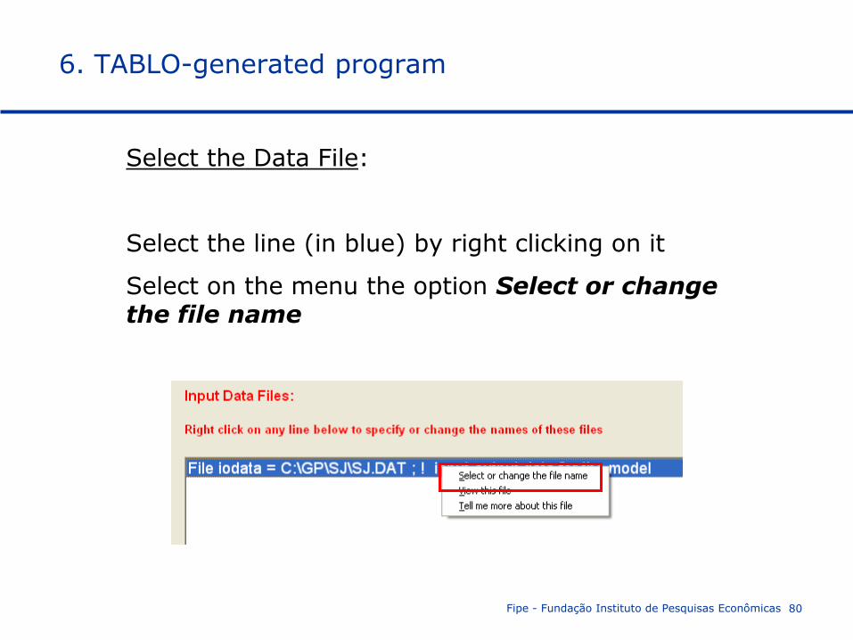
Select the Data File:
Select the line (in blue) by right clicking on it
Select on the menu the option Select or change the file name
6. TABLO-generated program
Fipe - Fundação Instituto de Pesquisas Econômicas 81
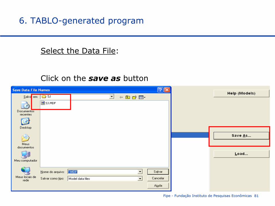
Select the Data File:
Click on the save as button
6. TABLO-generated program
Fipe - Fundação Instituto de Pesquisas Econômicas 82
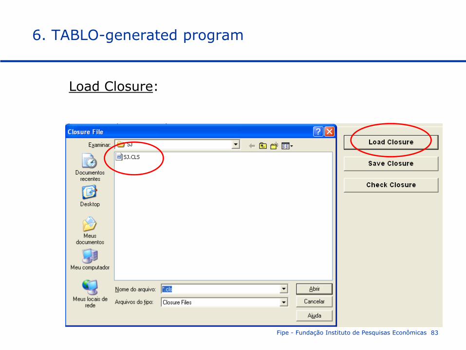
Load Closure:
Select the Closure link
Select the link Load Closure (as you have a closured saved in the SJ directory the GEMPACK will automatic open it).
If you do not have the file .CLS you can type the closure and save it.
exogenous p_FAC;
rest endogenous;
6. TABLO-generated program
Fipe - Fundação Instituto de Pesquisas Econômicas 83
Load Closure:
6. TABLO-generated program
Fipe - Fundação Instituto de Pesquisas Econômicas 84
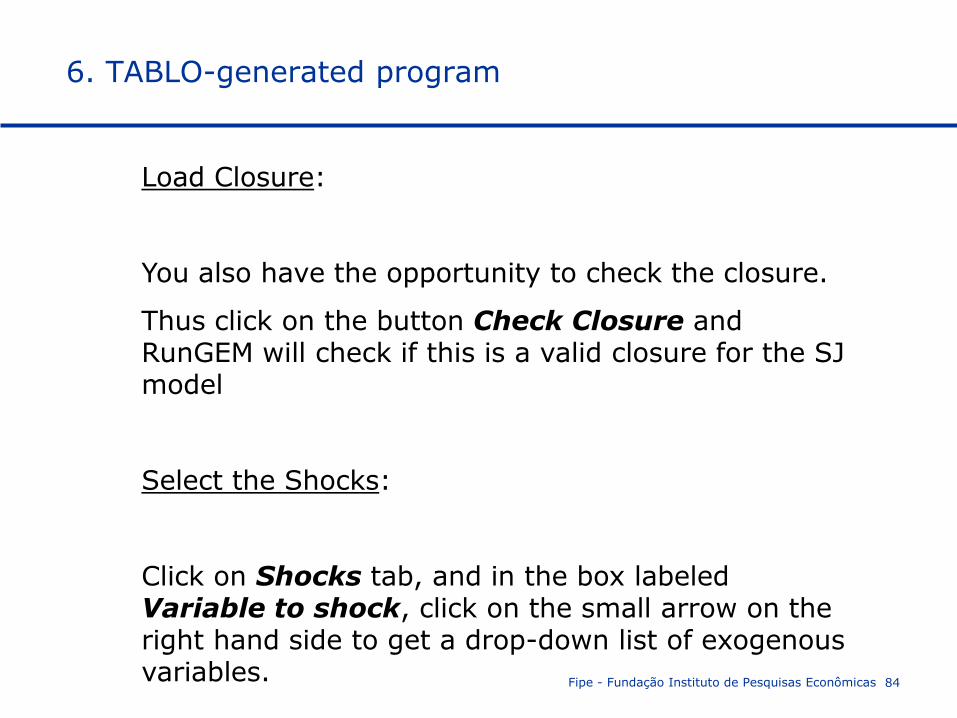
Load Closure:
You also have the opportunity to check the closure.
Thus click on the button Check Closure and RunGEM will check if this is a valid closure for the SJ model
Select the Shocks:
Click on Shocks tab, and in the box labeled Variable to shock, click on the small arrow on the right hand side to get a drop-down list of exogenous variables.
6. TABLO-generated program
Fipe - Fundação Instituto de Pesquisas Econômicas 85
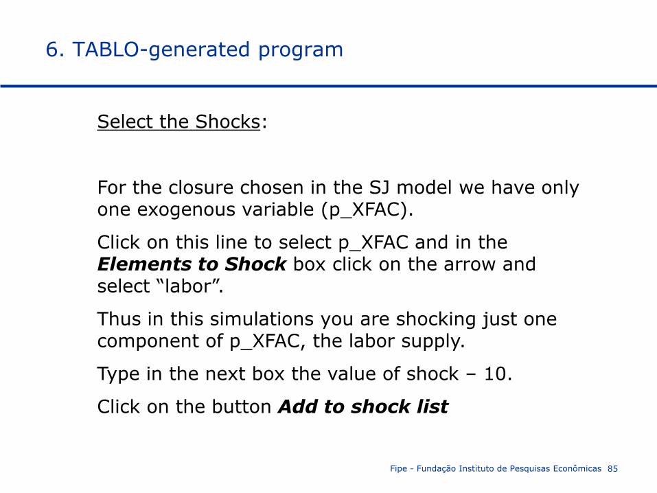
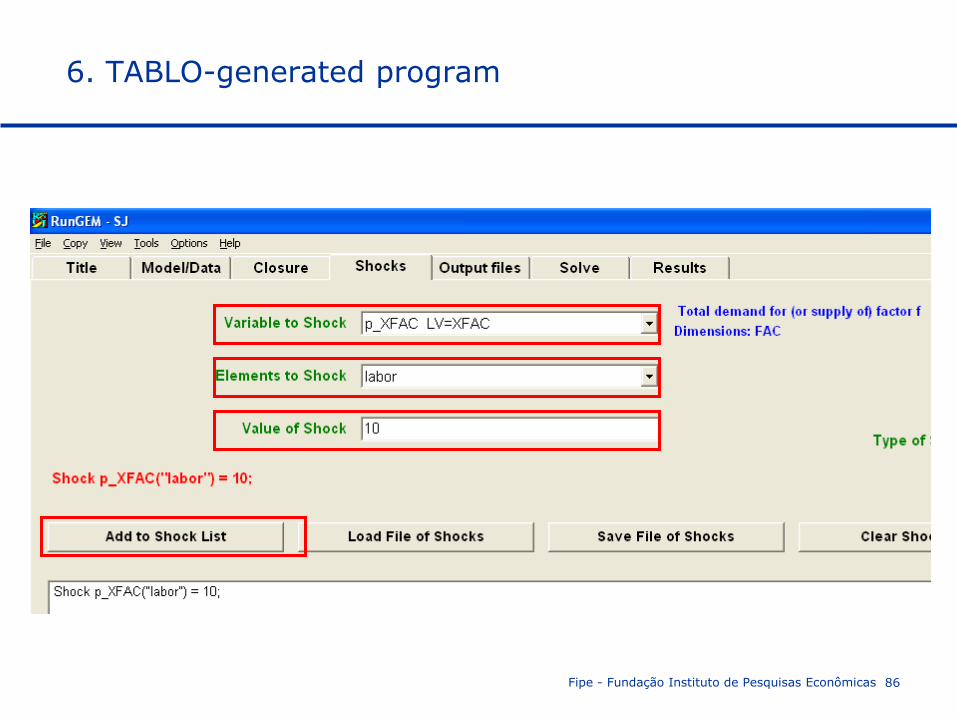
Select the Shocks:
For the closure chosen in the SJ model we have only one exogenous variable (p_XFAC).
Click on this line to select p_XFAC and in the Elements to Shock box click on the arrow and select “labor”.
Thus in this simulations you are shocking just one component of p_XFAC, the labor supply.
Type in the next box the value of shock – 10.
Click on the button Add to shock list
6. TABLO-generated program
Fipe - Fundação Instituto de Pesquisas Econômicas 86
6. TABLO-generated program
Fipe - Fundação Instituto de Pesquisas Econômicas 87
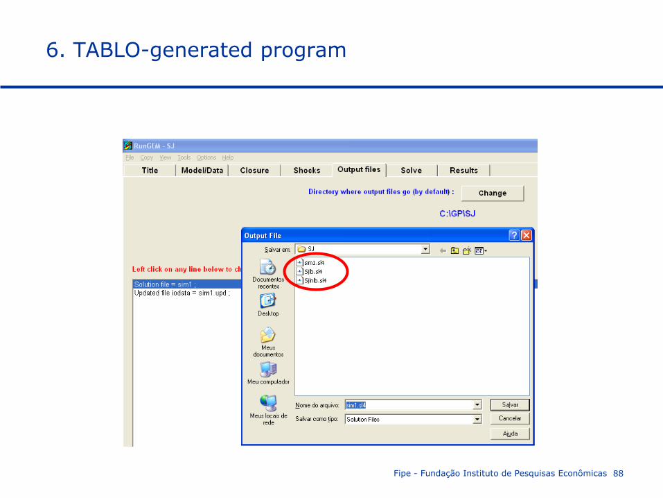
Output Files:
Click on Output files tab
To change the names of the output files, click (left click on this time) on the first line in the lower box:
Solution file = sim1.
Change the name of the Solution file to SJLB.SL4
6. TABLO-generated program
Fipe - Fundação Instituto de Pesquisas Econômicas 88
6. TABLO-generated program
Fipe - Fundação Instituto de Pesquisas Econômicas 89
Carry out a simulation:
Select the next page Solve and type in some verbal description to say
SJ. Standard closure – 10 percent increase in the labor supply
You need to select the solution method and steps.
Click on the Change button to the right of the text “Solution method”.
6. TABLO-generated program
Fipe - Fundação Instituto de Pesquisas Econômicas 90
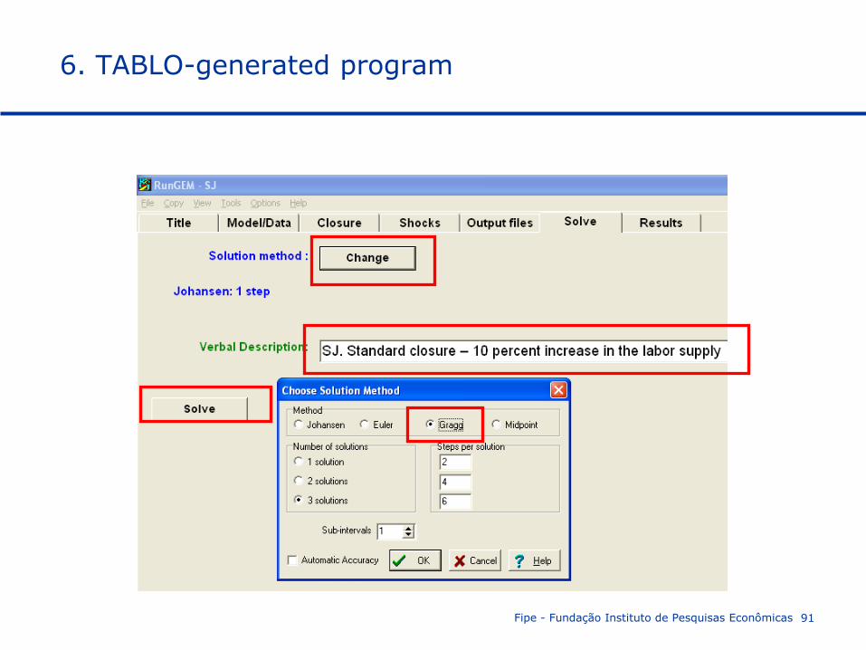
Carry out a simulation:
Select “Gragg’s method with 2,4,6 steps calculations [One subinterval, not automatic accuracy]
Click on the Solve button and the RunGEM will calculate a solution.
6. TABLO-generated program
Fipe - Fundação Instituto de Pesquisas Econômicas 91
6. TABLO-generated program
Fipe - Fundação Instituto de Pesquisas Econômicas 92
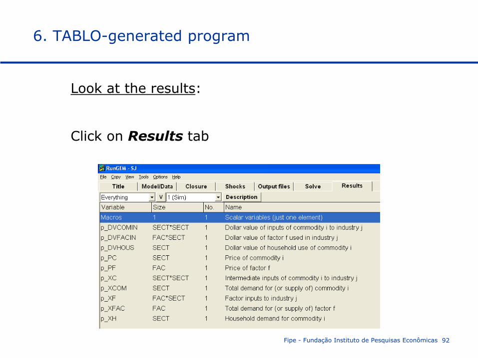
Look at the results:
Click on Results tab
6. TABLO-generated program
Fipe - Fundação Instituto de Pesquisas Econômicas 93
2.1.12. Different closures and/or shocks
2.1.13. Correcting errors in TABLO Input files
2.1.15. Creating the base data header array file
2.1.17. Condensing the model
Bonus. Sensitivity analysis to alternative functional forms to intermediate demands equations (Leontief versus Cobb-Douglas versus CES – sigma = 2)
Examples (GPD-8)