Australian Technical Guidelines for Monitoring and ...apvi.org.au/wp-content/uploads/2013/11/Australian... · Australian Technical Guidelines for Monitoring and Analysing Photovoltaic

November 2013

Jessie Copper1, Anna Bruce1, Ted Spooner2, Martina Calais3, Trevor Pryor3 and Muriel Watt1

1School of Photovoltaic and Renewable Energy Engineering, University of NSW

2School of Electrical Engineering and Telecommunications, University of NSW

33School of Engineering and Information Technology, Murdoch University

With the Support of:

Australian Technical Guidelines for Monitoring

and Analysing Photovoltaic Systems

Version 1.

1

GUIDELINE PREPARATION AND CONTACT INFORMATION

Guideline Prepared For:

The Australian Photovoltaic Institute (APVI) www.apvi.org.au

Contact:

Muriel Watt APVA Chair [email protected]

Guideline Prepared By:

Jessie Copper, Anna Bruce and Muriel Watt, School of Photovoltaic and Renewable Energy Engineering, University of NSW

Ted Spooner, School of Electrical and Telecommunications Engineering, University of NSW Martina Calais and Trevor Pryor, School of Engineering and Information Technology, Murdoch University

Guideline Reviewed By:

Lyndon Frearson and Paul Rodden, CAT Projects and additional anonymous reviewers

With the Support of:

http://www.apvi.org.au/

mailto:[email protected]

2

Contents

1 Executive Summary ....................................................................................................................... 4

2 Scope and Objectives .................................................................................................................... 9

3 Guidelines and Normative References ........................................................................................ 10

4 Nomenclature ............................................................................................................................. 11

5 Applications of PV System Monitoring ........................................................................................ 13

6 Measurement Specifications....................................................................................................... 15

6.1 Irradiance ............................................................................................................................ 18

6.1.1 Alternative Methods to Obtain Irradiance Data .......................................................... 19

6.2 Ambient air temperature .................................................................................................... 19

6.3 Wind speed ......................................................................................................................... 19

6.4 Module temperature .......................................................................................................... 20

6.5 Voltage, Current and Power ................................................................................................ 21

6.6 Measurement Sampling ...................................................................................................... 22

6.7 Recording and Monitoring Intervals .................................................................................... 24

6.8 Summary - Selecting the Appropriate Monitoring Strategy ................................................ 25

7 Reliability Specifications.............................................................................................................. 29

8 Performance Assessment............................................................................................................ 31

8.1 Check of Data Quality .......................................................................................................... 31

8.2 Derived Parameters ............................................................................................................ 31

8.3 Global Irradiation ................................................................................................................ 32

8.4 Electrical Energy Quantities ................................................................................................ 32

8.5 System Performance Indices ............................................................................................... 33

8.6 Yields ................................................................................................................................... 33

8.6.1 Normalised Losses ....................................................................................................... 33

8.6.2 Performance Ratio ...................................................................................................... 34

8.6.3 System Efficiencies ...................................................................................................... 34

8.7 Identifying Performance Issues ........................................................................................... 34

8.7.1 Graphical Analysis ....................................................................................................... 35

9 Appendices ................................................................................................................................. 38

9.1 Transposition Method of Horizontal Irradiance to In-plane Irradiance ............................... 38

9.2 Separation of Global Horizontal Irradiance into Direct and Diffuse Irradiance ................... 39

9.2.1 BRL Model ................................................................................................................... 39

9.2.2 Maxwell DISC Model ................................................................................................... 40

3

9.3 Module Temperature Models ............................................................................................. 40

9.3.1 Sandia Model .............................................................................................................. 40

9.3.2 Faiman Model ............................................................................................................. 41

9.4 Measurements at Installation ............................................................................................. 41

9.4.1 Analysis 1 – Clear Day Analysis .................................................................................... 42

9.4.2 Analysis 2 – Variation of Output across a Typical Day ................................................. 42

9.4.3 Analysis 3 – Other Days Analysis ................................................................................. 42

9.4.4 Analysis 4 – Inverter Measurements ........................................................................... 42

10 References .............................................................................................................................. 44

4

1 Executive Summary

Monitoring of photovoltaic systems is required for the detection of operational issues, and to compare the performance of different systems across a range of technologies and climates. Performance and reliability data can therefore facilitate appropriate system design and technology choice, and in the long term, establish credible expectations about PV system performance.

The purpose of this guideline is to provide recommendations for monitoring and analysis of the performance and reliability of flat plate grid connected photovoltaic (PV) systems in Australia.

This guideline was developed primarily with reference to the following documents, with adaptations for current and emerging needs and Australian conditions:

IEC Standard 61724: Photovoltaic system performance monitoring – Guidelines for measurement, data exchange and analysis

European Commission 6th Framework Programme: Monitoring guidelines for photovoltaic systems

This document offers guidance on which parameters should be measured, how they should be measured and the frequency of measurement for the following seven uses of PV performance and reliability data:

1. Performance assessment of PV technologies under outdoor conditions

a. Basic monitoring

b. Detailed monitoring

2. Performance diagnostics

3. Degradation and uncertainty analysis with time

4. Understanding/reducing system losses via comparisons to modelled performance data

5. Forecasting PV performance

6. Interaction of PV systems with the electricity network

7. Integration of distributed generation, storage and load control

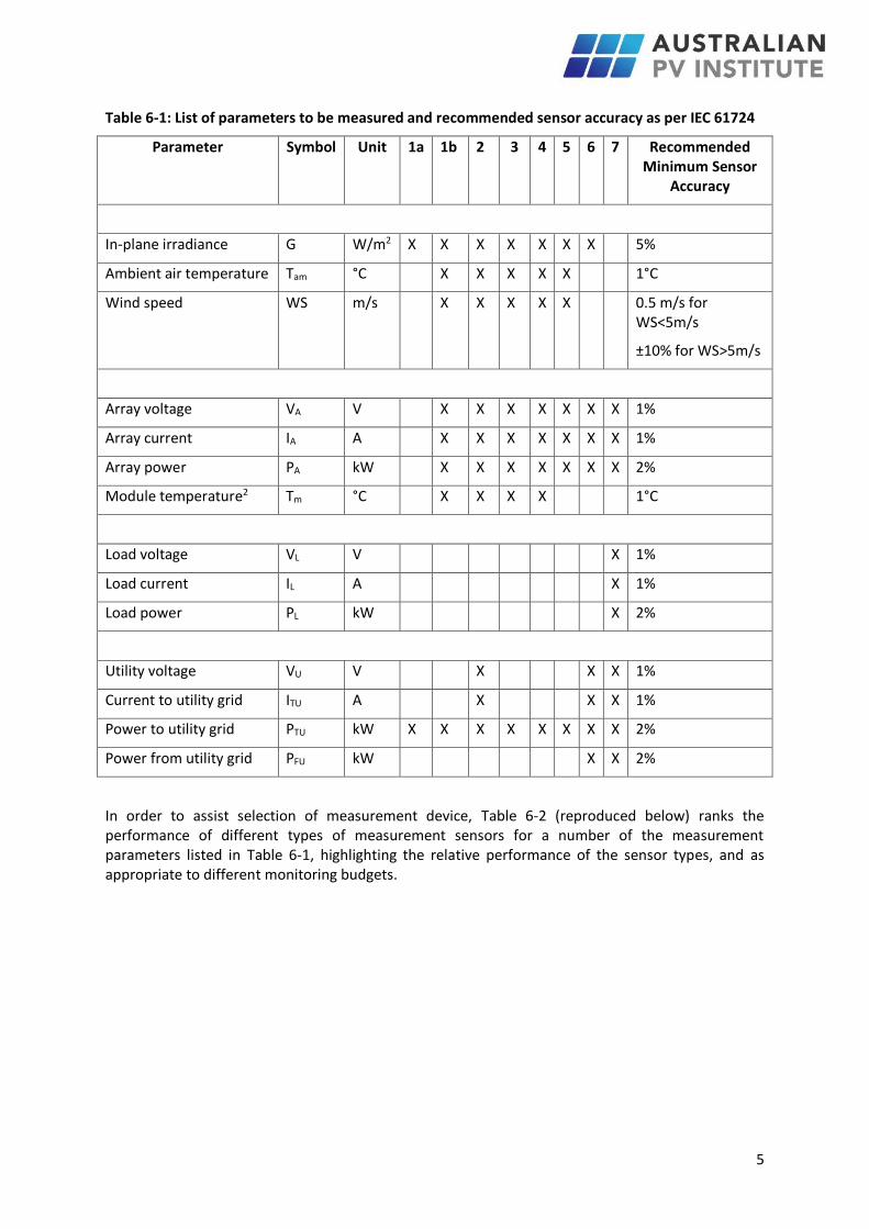
Table 6-1 (reproduced below) identifies which parameters should be measured for each of the applications 1-7 listed above, together with their recommended sensor accuracy.

5

Table 6-1: List of parameters to be measured and recommended sensor accuracy as per IEC 61724

Parameter Symbol Unit 1a 1b 2 3 4 5 6 7 Recommended Minimum Sensor

Accuracy

In-plane irradiance G W/m2 X X X X X X X 5%

Ambient air temperature Tam °C X X X X X 1°C

Wind speed WS m/s X X X X X 0.5 m/s for WS<5m/s

±10% for WS>5m/s

Array voltage VA V X X X X X X X 1%

Array current IA A X X X X X X X 1%

Array power PA kW X X X X X X X 2%

Module temperature2 Tm °C X X X X 1°C

Load voltage VL V X 1%

Load current IL A X 1%

Load power PL kW X 2%

Utility voltage VU V X X X 1%

Current to utility grid ITU A X X X 1%

Power to utility grid PTU kW X X X X X X X X 2%

Power from utility grid PFU kW X X 2%

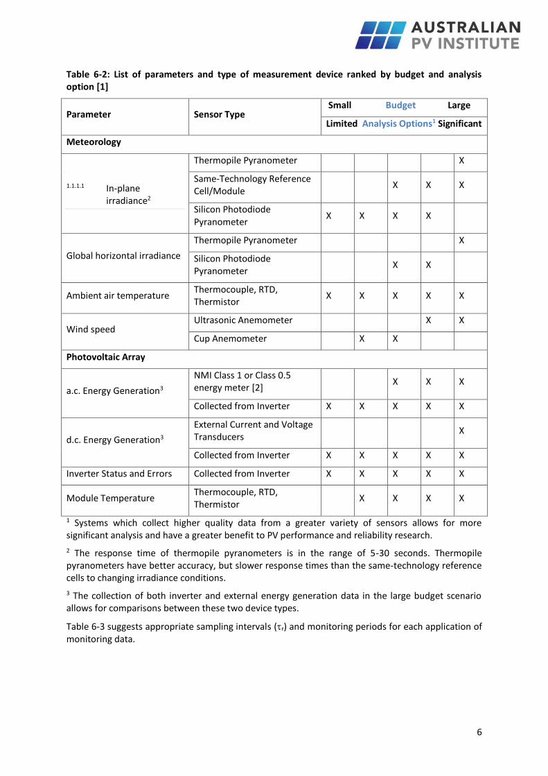
In order to assist selection of measurement device, Table 6-2 (reproduced below) ranks the performance of different types of measurement sensors for a number of the measurement parameters listed in Table 6-1, highlighting the relative performance of the sensor types, and as appropriate to different monitoring budgets.

6

Table 6-2: List of parameters and type of measurement device ranked by budget and analysis option [1]

Parameter Sensor Type Small Budget Large

Limited Analysis Options1 Significant

Meteorology

1.1.1.1 In-plane irradiance2

Thermopile Pyranometer X

Same-Technology Reference Cell/Module

X X X

Silicon Photodiode Pyranometer

X X X X

Global horizontal irradiance



X X

Ambient air temperature Thermocouple, RTD, Thermistor

X X X X X

Wind speed Ultrasonic Anemometer X X

Cup Anemometer X X

Photovoltaic Array

a.c. Energy Generation3

NMI Class 1 or Class 0.5 energy meter [2]

X X X

Collected from Inverter X X X X X

d.c. Energy Generation3

External Current and Voltage Transducers

X


Inverter Status and Errors Collected from Inverter X X X X X

Module Temperature Thermocouple, RTD, Thermistor

X X X X

1 Systems which collect higher quality data from a greater variety of sensors allows for more significant analysis and have a greater benefit to PV performance and reliability research.

2 The response time of thermopile pyranometers is in the range of 5-30 seconds. Thermopile pyranometers have better accuracy, but slower response times than the same-technology reference cells to changing irradiance conditions.

3 The collection of both inverter and external energy generation data in the large budget scenario allows for comparisons between these two device types.

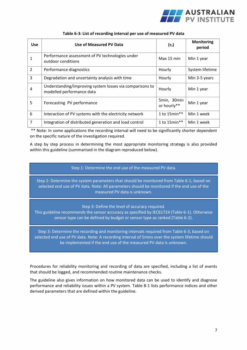
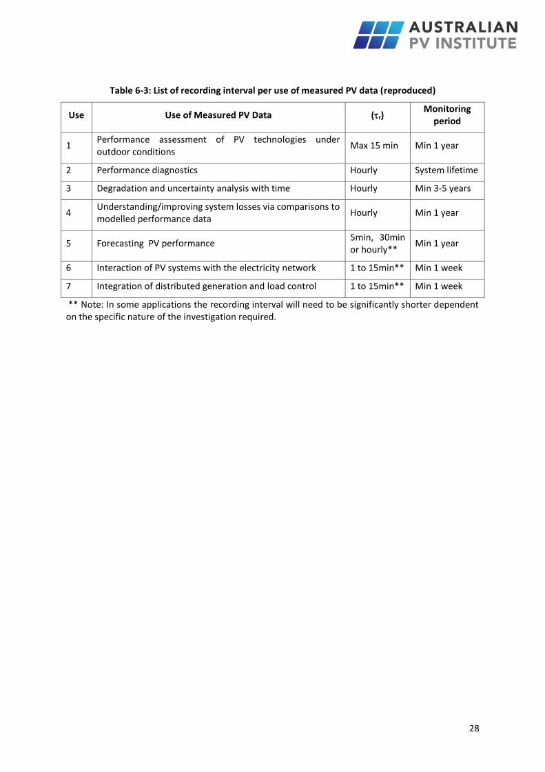
Table 6-3 suggests appropriate sampling intervals (r) and monitoring periods for each application of monitoring data.

7

Table 6-3: List of recording interval per use of measured PV data

Use Use of Measured PV Data (r) Monitoring

period

1 Performance assessment of PV technologies under outdoor conditions

Max 15 min Min 1 year

2 Performance diagnostics Hourly System lifetime

3 Degradation and uncertainty analysis with time Hourly Min 3-5 years

4 Understanding/improving system losses via comparisons to modelled performance data

Hourly Min 1 year

5 Forecasting PV performance 5min, 30min or hourly**

Min 1 year

6 Interaction of PV systems with the electricity network 1 to 15min** Min 1 week

7 Integration of distributed generation and load control 1 to 15min** Min 1 week

** Note: In some applications the recording interval will need to be significantly shorter dependent on the specific nature of the investigation required.

A step by step process in determining the most appropriate monitoring strategy is also provided within this guideline (summarised in the diagram reproduced below).

Procedures for reliability monitoring and recording of data are specified, including a list of events that should be logged, and recommended routine maintenance checks.

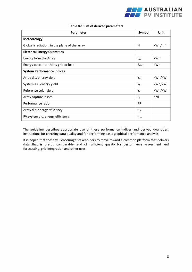
The guideline also gives information on how monitored data can be used to identify and diagnose performance and reliability issues within a PV system. Table 8-1 lists performance indices and other derived parameters that are defined within the guideline.

Step 1: Determine the end use of the measured PV data.

Step 2: Determine the system parameters that should be monitored from Table 6-1, based on selected end use of PV data. Note: All parameters should be monitored if the end use of the

measured PV data is unknown.

Step 3: Define the level of accuracy required. This guideline recommends the sensor accuracy as specified by IEC61724 (Table 6-1). Otherwise

sensor type can be defined by budget or sensor type as ranked (Table 6-2).

Step 3: Determine the recording and monitoring intervals required from Table 6-3, based on selected end use of PV data. Note: A recording interval of 5mins over the system lifetime should

be implemented if the end use of the measured PV data is unknown.

8

Table 8-1: List of derived parameters

Parameter Symbol Unit

Meteorology

Global irradiation, in the plane of the array H kWh/m2

Electrical Energy Quantities

Energy from the Array EA kWh

Energy output to Utility grid or load Eout kWh

System Performance Indices

Array d.c. energy yield YA kWh/kW

System a.c. energy yield Yf kWh/kW

Reference solar yield Yr kWh/kW

Array capture losses Lc h/d

Performance ratio PR

Array d.c. energy efficiency A

PV system a.c. energy efficiency pv

The guideline describes appropriate use of these performance indices and derived quantities; instructions for checking data quality and for performing basic graphical performance analysis.

It is hoped that these will encourage stakeholders to move toward a common platform that delivers data that is useful, comparable, and of sufficient quality for performance assessment and forecasting, grid integration and other uses.

9

2 Scope and Objectives

The purpose of this guideline is to provide recommendations for monitoring and analysis of the performance and reliability of flat plate grid connected photovoltaic (PV) systems. It does not cover issues specifically associated with stand-alone, tracking, concentrator or building integrated1 PV systems. Appropriate parameters to measure, accuracy and frequency of measurement vary for different applications of PV performance and reliability data. This document offers guidance on which parameters should be measured, how they should be measured and the frequency of measurement for the following 7 uses of PV performance and reliability data.


Either basic or detailed monitoring

2. Performance Diagnostics




6. Interaction of PV systems with electricity networks


A step by step process for determining the most appropriate monitoring strategy is provided. Procedures for the analysis of monitored data in order to identify and diagnose performance and reliability issues within a PV system are provided, including agreed definitions for performance indices and other derived parameters; appropriate use of these; instructions for checking data quality and for performing basic graphical performance analysis.

1 Within this guideline building integrated PV systems refers to PV systems where the PV modules within the system perform additional functions in addition to generating electricity. The design of building integrated systems may compromise on the PV performance to obtain other benefits from the system which would require additional measurement metrics to ascertain both the performance of the PV system electrically and with regards to other functions. PV systems that are mounted on existing building structures are not considered to be building integrated, and hence are covered by the content within this guideline.

10

3 Guidelines and Normative References

This guideline was developed primarily with reference to the following documents, with adaptations for current and emerging needs and Australian conditions:

IEC Standard 61724: Photovoltaic system performance monitoring – Guidelines for

measurement, data exchange and analysis

European Commission 6th Framework Programme: Monitoring guidelines for photovoltaic

systems

The following documents, have also been used as references:

• DERlab TG 100-01: Technical guidelines on long-term photovoltaic module outdoor tests

• IEC 60904-2: Photovoltaic devices – Part 2: Requirements for reference solar devices

• IEC 60904-6: Photovoltaic devices – Part 6: Requirements for reference solar modules

• IEC 61215: Crystalline silicon terrestrial photovoltaic (PV) modules – Design qualification and

type approval

• IEC 61829: Crystalline silicon photovoltaic (PV) array – On-site measurement of I-V

characteristics

• NMI M 6-1 Electricity Meters Part 1: Metrological and Technical Requirements.

• WMO, No. 8: Guide to meteorological Instruments and Methods of Observation: (CIMO

guide)

11

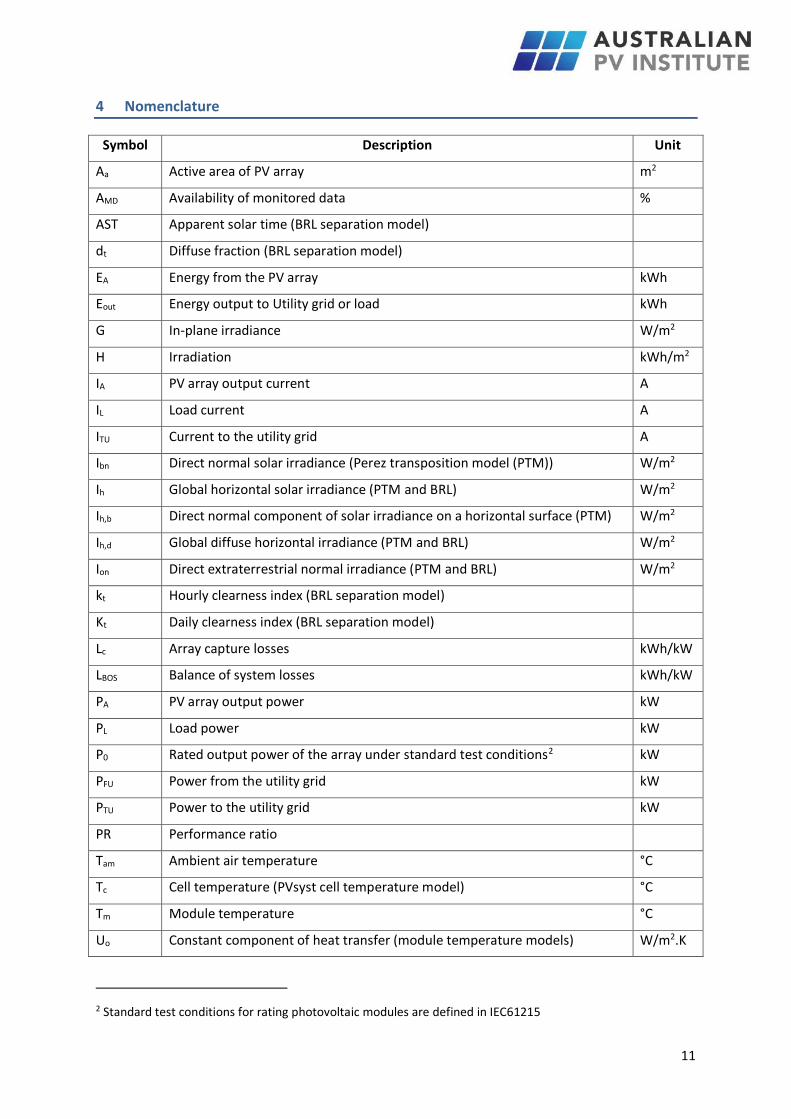
4 Nomenclature

Symbol Description Unit

Aa Active area of PV array m2

AMD Availability of monitored data %

AST Apparent solar time (BRL separation model)

dt Diffuse fraction (BRL separation model)

EA Energy from the PV array kWh

Eout Energy output to Utility grid or load kWh

G In-plane irradiance W/m2

H Irradiation kWh/m2

IA PV array output current A

IL Load current A

ITU Current to the utility grid A

Ibn Direct normal solar irradiance (Perez transposition model (PTM)) W/m2

Ih Global horizontal solar irradiance (PTM and BRL) W/m2

Ih,b Direct normal component of solar irradiance on a horizontal surface (PTM) W/m2

Ih,d Global diffuse horizontal irradiance (PTM and BRL) W/m2

Ion Direct extraterrestrial normal irradiance (PTM and BRL) W/m2

kt Hourly clearness index (BRL separation model)

Kt Daily clearness index (BRL separation model)

Lc Array capture losses kWh/kW

LBOS Balance of system losses kWh/kW

PA PV array output power kW

PL Load power kW

P0 Rated output power of the array under standard test conditions2 kW

PFU Power from the utility grid kW

PTU Power to the utility grid kW

PR Performance ratio

Tam Ambient air temperature °C

Tc Cell temperature (PVsyst cell temperature model) °C

Tm Module temperature °C

Uo Constant component of heat transfer (module temperature models) W/m2.K

2 Standard test conditions for rating photovoltaic modules are defined in IEC61215

12

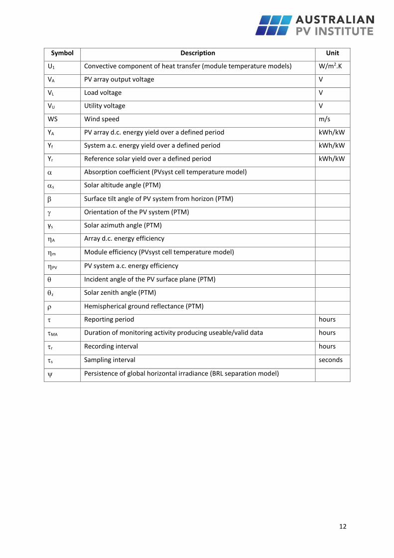
Symbol Description Unit

U1 Convective component of heat transfer (module temperature models) W/m2.K

VA PV array output voltage V

VL Load voltage V

VU Utility voltage V

WS Wind speed m/s

YA PV array d.c. energy yield over a defined period kWh/kW

Yf System a.c. energy yield over a defined period kWh/kW

Yr Reference solar yield over a defined period kWh/kW

Absorption coefficient (PVsyst cell temperature model)

s Solar altitude angle (PTM)

Surface tilt angle of PV system from horizon (PTM)

Orientation of the PV system (PTM)

γs Solar azimuth angle (PTM)

A Array d.c. energy efficiency

m Module efficiency (PVsyst cell temperature model)

PV PV system a.c. energy efficiency

Incident angle of the PV surface plane (PTM)

z Solar zenith angle (PTM)

Hemispherical ground reflectance (PTM)

Reporting period hours

MA Duration of monitoring activity producing useable/valid data hours

r Recording interval hours

s Sampling interval seconds

Persistence of global horizontal irradiance (BRL separation model)

13

5 Applications of PV System Monitoring

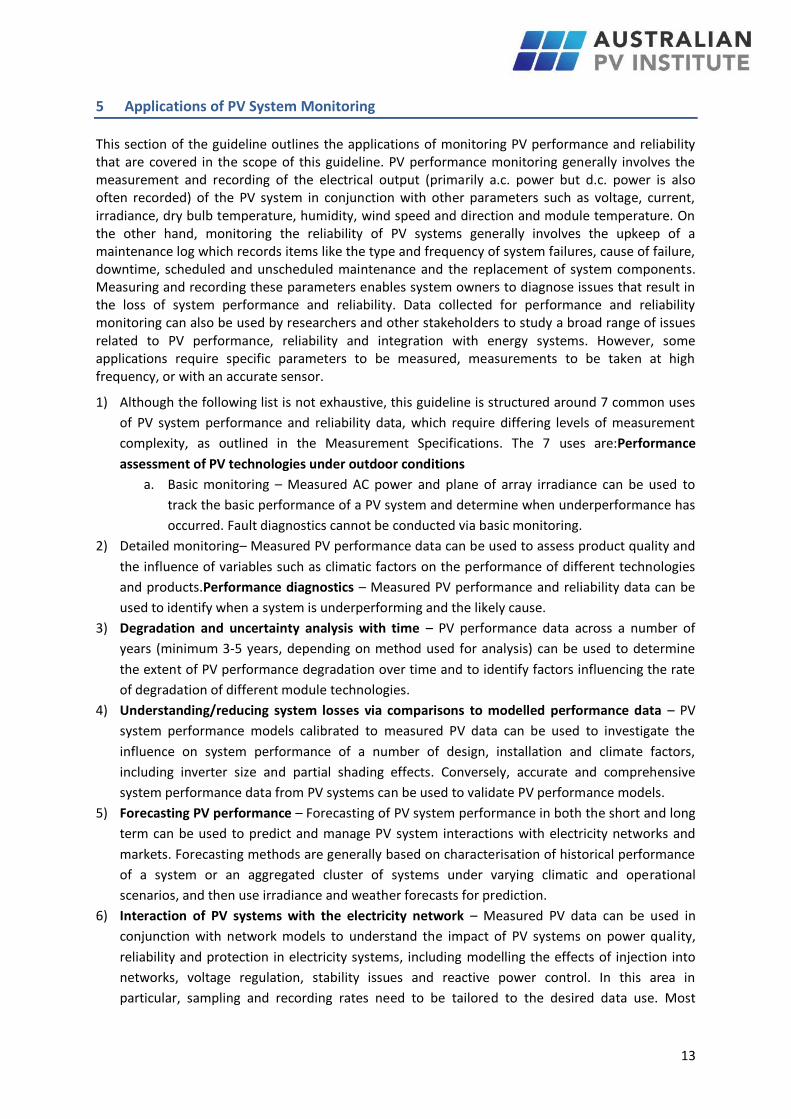
This section of the guideline outlines the applications of monitoring PV performance and reliability that are covered in the scope of this guideline. PV performance monitoring generally involves the measurement and recording of the electrical output (primarily a.c. power but d.c. power is also often recorded) of the PV system in conjunction with other parameters such as voltage, current, irradiance, dry bulb temperature, humidity, wind speed and direction and module temperature. On the other hand, monitoring the reliability of PV systems generally involves the upkeep of a maintenance log which records items like the type and frequency of system failures, cause of failure, downtime, scheduled and unscheduled maintenance and the replacement of system components. Measuring and recording these parameters enables system owners to diagnose issues that result in the loss of system performance and reliability. Data collected for performance and reliability monitoring can also be used by researchers and other stakeholders to study a broad range of issues related to PV performance, reliability and integration with energy systems. However, some applications require specific parameters to be measured, measurements to be taken at high frequency, or with an accurate sensor.

1) Although the following list is not exhaustive, this guideline is structured around 7 common uses

of PV system performance and reliability data, which require differing levels of measurement

complexity, as outlined in the Measurement Specifications. The 7 uses are:Performance

assessment of PV technologies under outdoor conditions

a. Basic monitoring – Measured AC power and plane of array irradiance can be used to

track the basic performance of a PV system and determine when underperformance has

occurred. Fault diagnostics cannot be conducted via basic monitoring.

2) Detailed monitoring– Measured PV performance data can be used to assess product quality and

the influence of variables such as climatic factors on the performance of different technologies

and products.Performance diagnostics – Measured PV performance and reliability data can be

used to identify when a system is underperforming and the likely cause.

3) Degradation and uncertainty analysis with time – PV performance data across a number of

years (minimum 3-5 years, depending on method used for analysis) can be used to determine

the extent of PV performance degradation over time and to identify factors influencing the rate

of degradation of different module technologies.

4) Understanding/reducing system losses via comparisons to modelled performance data – PV

system performance models calibrated to measured PV data can be used to investigate the

influence on system performance of a number of design, installation and climate factors,

including inverter size and partial shading effects. Conversely, accurate and comprehensive

system performance data from PV systems can be used to validate PV performance models.

5) Forecasting PV performance – Forecasting of PV system performance in both the short and long

term can be used to predict and manage PV system interactions with electricity networks and

markets. Forecasting methods are generally based on characterisation of historical performance

of a system or an aggregated cluster of systems under varying climatic and operational

scenarios, and then use irradiance and weather forecasts for prediction.

6) Interaction of PV systems with the electricity network – Measured PV data can be used in

conjunction with network models to understand the impact of PV systems on power quality,

reliability and protection in electricity systems, including modelling the effects of injection into

networks, voltage regulation, stability issues and reactive power control. In this area in

particular, sampling and recording rates need to be tailored to the desired data use. Most

14

challenging in terms of PV data requirements is the study of variability of PV output over very

short timeframes, and spatially across large systems or a number of distributed systems, which

enables assessment of the impact of climatic effects like sharp cloud boundaries on the stability

of the generated power.

7) Integration of distributed generation, storage and load control – Monitored PV data can be

used to examine issues related to the combination of PV systems with other distributed energy

technologies into electricity systems. Monitored PV data may be used to assess the need for

energy storage and/or load shifting to allow higher values of penetration.

Each of the above mentioned uses of PV data require different levels of measurement complexity. This guideline provides details on the parameters and frequency of measurement for each of the above listed uses of PV data.

15

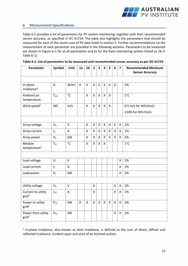
6 Measurement Specifications

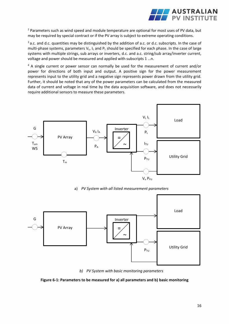
Table 6-1 provides a list of parameters for PV system monitoring, together with their recommended sensor accuracy, as specified in IEC 61724. The table also highlights the parameters that should be measured for each of the seven uses of PV data listed in section 5. Further recommendations on the measurement of each parameter are provided in the following sections. Parameters to be measured are shown in Figure 6-1 for a) all parameters and b) for the basic monitoring system (listed as 1b in Table 6-1).

Table 6-1: List of parameters to be measured and recommended sensor accuracy as per IEC 61724

Parameter Symbol Unit 1a 1b 2 3 4 5 6 7 Recommended Minimum Sensor Accuracy

In-plane irradiance1

G W/m2 X X X X X X X 5%

Ambient air temperature

Tam °C X X X X X 1°C

Wind speed2 WS m/s X X X X X 0.5 m/s for WS<5m/s

±10% for WS>5m/s




Module temperature2

Tm °C X X X X 1°C





Current to utility grid4

ITU A X X X 1%

Power to utility grid4

PTU kW X X X X X X X X 2%

Power from utility grid4

PFU kW X X 2%

1 In-plane irradiance, also known as total irradiance, is defined as the sum of direct, diffuse and reflected irradiance, incident upon unit area of an inclined surface.

16

2 Parameters such as wind speed and module temperature are optional for most uses of PV data, but may be required by special contract or if the PV array is subject to extreme operating conditions.

3 a.c. and d.c. quantities may be distinguished by the addition of a.c. or d.c. subscripts. In the case of multi-phase systems, parameters VL, IL and PL should be specified for each phase. In the case of large systems with multiple strings, sub arrays or inverters, d.c. and a.c. string/sub array/inverter current, voltage and power should be measured and applied with subscripts 1 …n.

4 A single current or power sensor can normally be used for the measurement of current and/or power for directions of both input and output. A positive sign for the power measurement represents input to the utility grid and a negative sign represents power drawn from the utility grid. Further, it should be noted that any of the power parameters can be calculated from the measured data of current and voltage in real time by the data acquisition software, and does not necessarily require additional sensors to measure these parameters.

a) PV System with all listed measurement parameters

b) PV System with basic monitoring parameters

Figure 6-1: Parameters to be measured for a) all parameters and b) basic monitoring

Load

VA IA

PA

VL IL

PL

ITU

PTU Utility Grid

Vu PFU

Inverter

= ~

PV Array

Tm

G

Tam WS

Load

PTU Utility Grid

Inverter

= ~

PV Array

G

17

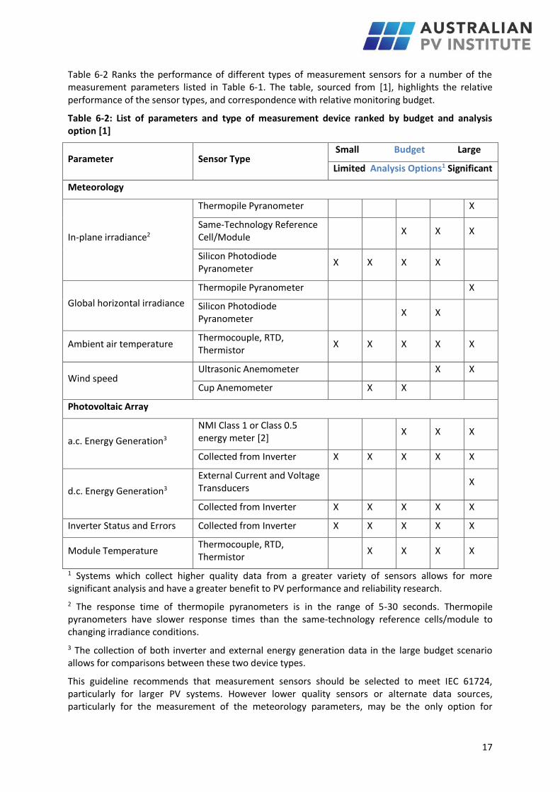
Table 6-2 Ranks the performance of different types of measurement sensors for a number of the measurement parameters listed in Table 6-1. The table, sourced from [1], highlights the relative performance of the sensor types, and correspondence with relative monitoring budget.

Table 6-2: List of parameters and type of measurement device ranked by budget and analysis option [1]



Meteorology

In-plane irradiance2



X X X


X X X X




X X


X X X X X


Cup Anemometer X X

Photovoltaic Array



X X X




X




X X X X


2 The response time of thermopile pyranometers is in the range of 5-30 seconds. Thermopile pyranometers have slower response times than the same-technology reference cells/module to changing irradiance conditions.


This guideline recommends that measurement sensors should be selected to meet IEC 61724, particularly for larger PV systems. However lower quality sensors or alternate data sources, particularly for the measurement of the meteorology parameters, may be the only option for

18

smaller PV systems with lower performance monitoring budgets. It should be noted that use of monitored performance data from systems with higher quality sensors is more valuable for research purposes and improves performance diagnostic capabilities.

Where the inverter has data collection functionality built in, it is important to compare the accuracy of the measurement sensors with the recommendations given here. Modern inverters commonly have capabilities to measure the d.c. and a.c. voltage, current and power from the PV array and power imported from and exported to the grid. This facility may reduce the need for additional sensors and hence the cost of a monitoring system, however the accuracy of the measurement undertaken by the Inverter should be checked against the requirements of IEC 61724. Most modern day inverters do not meet IEC 61724 requirements, hence inverter monitoring will reduce the ability to identify system performance issues. Monitoring of voltage, current and power parameters via an inverter is not recommended if financial decisions/calculations are required from the monitored data for contractual agreements.

6.1 Irradiance

The electrical output of photovoltaic systems is directly correlated to the incident level of irradiance on the surface of the modules. To effectively determine whether the PV system is operating according to design it is essential to have a measurement of the level of irradiance. The definition of irradiance is the instantaneous measurement of solar power on a surface in W/m2, whilst irradiation is the sum of solar energy on the surface over a defined period in Wh/m2 or kWh/m2.

For the most rigorous measurements, it is recommended that in-plane irradiance is measured according to IEC 61724. This requires the measurement of irradiance in the same plane as the photovoltaic array by means of a calibrated reference device or pyranometer. If used, reference devices should be calibrated and maintained in accordance with IEC 60904-2 or IEC 60904-6 as appropriate and, where possible, should be spectrally matched to the monitored PV array. The accuracy of the irradiance sensors, including signal condition, according to IEC 61724 should be better than 5%.

The type of sensor used to measure irradiance is largely dependent on the level of monitoring accuracy required and the budget specified for the monitoring system. Table 6-2 ranks the performance of different types of measurement sensors for a number of the measurement parameters listed in Table 6-1. The table, sourced from [1], highlights the relative performance of the sensor types, and correspondence with relative monitoring budget. It should be noted that although the thermopile pyranometers are the most accurate sensors listed in Table 6-2, they have slower response times to changes in irradiance conditions (between 5-30 seconds) in comparison to the same-technology reference devices and PV modules. The choice of irradiance sensor is therefore also dependent on the use of the measured data. Research presented in [3, 4] recommends that thermopile pyranometers should be used for PV performance monitoring. However same-technology reference devices would be the preferred method of irradiance measurement if variability effects of PV are to be investigated (use 6 in Table 6-3).

On-site measurements of irradiance will provide the highest level of accuracy, providing that appropriate calibration, installation and maintenance procedures of the sensors are carried out. Many high quality pyranometers require periodic calibration (approximately every 2 years) which often entails sending the pyranometers away to be calibrated. Such issues must be considered in maintenance planning if data gaps are to be avoided.

Regardless of sensor type and accuracy, the location of any measurement sensor should be representative of the irradiance conditions of the array. The sensor should be co-planar with the modules of the array with a maximum deviation of 2°. The sensor should be positioned where it is unshaded at all times (regardless of whether the PV array is partially shaded at any time) and in a location where it can be accessed for cleaning at regular intervals.

19

6.1.1 Alternative Methods to Obtain Irradiance Data

This guideline recommends that measurement sensors should be selected to meet IEC 61724, particularly for larger PV systems. However lower quality sensors or alternate data sources, particularly for the measurement of the meteorology parameters, may be the only option for smaller PV systems with lower performance monitoring budgets. It should be noted that use of monitored performance data from systems with higher quality sensors is more valuable for research purposes and improves performance diagnostic capabilities.

For smaller PV systems (typically smaller than 5kWp), in-plane irradiance may be either (1) measured on site (recommended method), (2) measured at another location chosen to be representative or (3) derived from remote measurements and/or synthesised from a combination of ground measured irradiance data and satellite data (e.g. the Australian Bureau of Meteorology gridded solar data set), depending on the accuracy requirements.

Use of satellite derived irradiance data may be used to infer in-plane irradiance for small PV systems where the expense and technical requirements of installing and maintaining on-site irradiance sensor(s) cannot be justified. Satellite derived irradiance is typically reported for a horizontal plane; hence a recognised method of translation to irradiance in the plane of the array must be used. The recommended method for this translation is the Perez model [5, 6] which is detailed in the appendices. It should also be noted that reduced accuracy resulting from estimates of in-plane irradiance via a transposition model, and particularly if satellite derived horizontal irradiance is used as input into the transposition model, will reduce its usefulness, for instance for identifying system loss factors. In addition satellite derived irradiance is unlikely to be reported at a measurement frequency less than an hour.

Note: On-site measurement of in-plane irradiance is the recommended option regardless of system size.

6.2 Ambient air temperature

Ambient air temperature, measured in degrees Celsius (°C), in conjunction with in-plane irradiance and wind speed are typically used in PV performance monitoring and modelling to estimate module efficiency losses due to changes in module temperatures in comparison to standard test conditions (25°C).

Again, for the most rigorous level of measurement, it is recommended that ambient air temperature should be measured according to IEC 61724. This requires that ambient temperature should be measured at a location that is representative of the array conditions, by means of temperature sensors housed in solar radiation shields. Radiation shields are required in order to ensure that the temperature sensor measures the air temperature only and is not heated by direct irradiance from the sun or cooled due to wind effects. Temperature sensors should be positioned away from any heat sources and, where possible, at least 1m above the ground. The DERlab TG 100-01 guideline recommends a position of 2m above the ground. The accuracy of air temperature sensors, including signal conditioning, according to IEC 61724 should be better than 1°C.

6.3 Wind speed

Wind speed, measured in m/s, affects the performance of PV systems by increasing convective heat loss, and reducing the temperature of the PV modules. Wind speed is a less significant determinant of system performance than ambient temperature, and it is thus a less important parameter to measure; however it is a useful parameter to improve the accuracy of module temperature estimates and therefore system performance analysis if on-site measurements of module temperatures are not recorded. Wind speed should be measured if the array is subjected to extreme weather conditions.

20

Again, for the most rigorous level of measurement, it is recommended that wind speed be measured according to IEC 61724. This requires that wind speed should be measured at a height and location that is representative of the array conditions. The accuracy of wind speed sensors should be better

than 0.5m/s for wind speeds 5m/s, and better than 10% of the measurement for wind speeds 5m/s. Ideally installation of a wind speed sensor (anemometer) should be, according to IEC 61215, at 1.2m distance on the East or West side of the system and at 0.7m above the upper edge of the system.

6.4 Module temperature

Module temperature, measured in degrees Celsius (°C), is a recommended measurement parameter, as the performance of PV systems is directly correlated to the operating temperature of the modules. The impact of module temperature on PV system performance is dependent on the PV technology employed in the system. Typically crystalline and multi-crystalline silicon technologies suffer significant performance losses due to temperature effects.

Again for the most rigorous level of measurement, it is recommended that module temperature be measured according to IEC 61724. This requires that module temperature should be measured at locations which are representative of the array conditions by means of temperature sensors located on the back surface of one or more modules. It is noted that care must be taken to ensure that the temperature of the cell in front of the sensor is not substantially altered due to the presence of the sensor. The accuracy of these sensors, including signal processing, according to IEC 61724 should be better than 1°C.

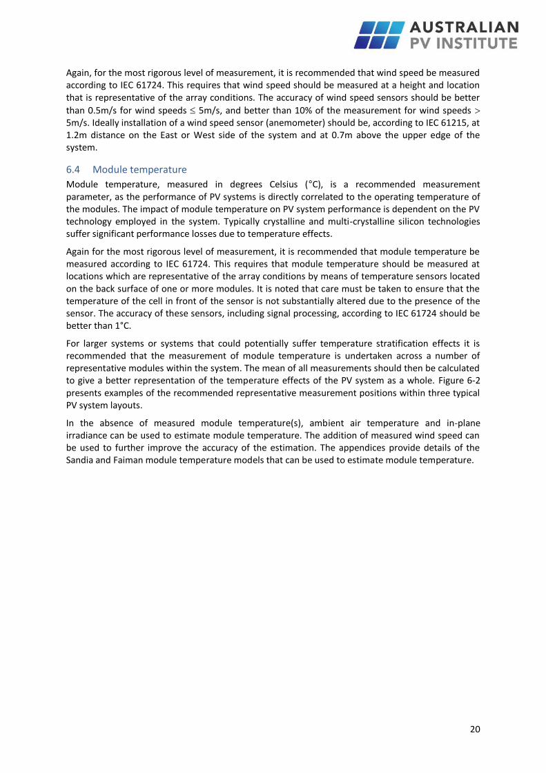
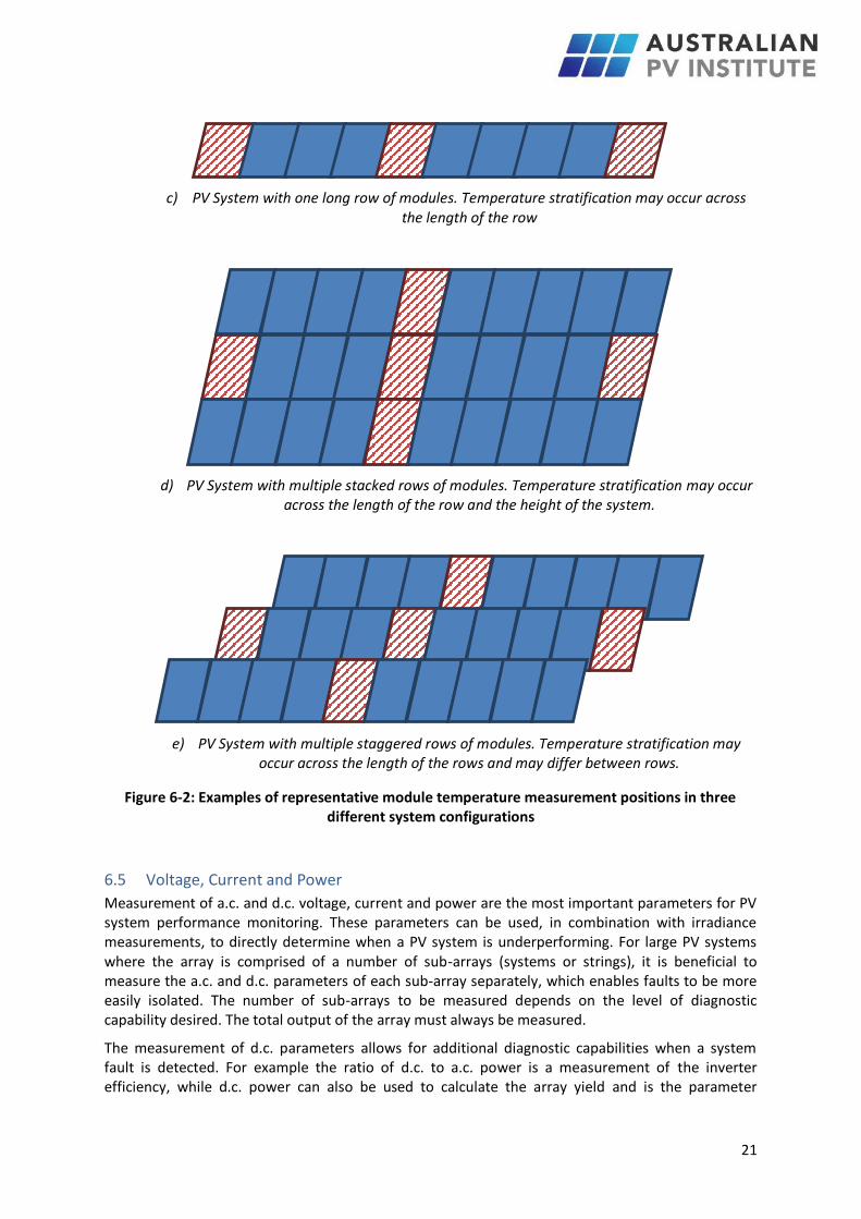
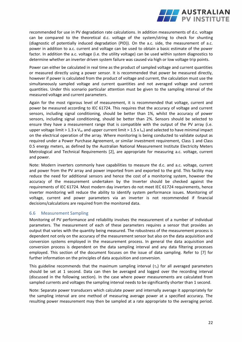
For larger systems or systems that could potentially suffer temperature stratification effects it is recommended that the measurement of module temperature is undertaken across a number of representative modules within the system. The mean of all measurements should then be calculated to give a better representation of the temperature effects of the PV system as a whole. Figure 6-2 presents examples of the recommended representative measurement positions within three typical PV system layouts.

In the absence of measured module temperature(s), ambient air temperature and in-plane irradiance can be used to estimate module temperature. The addition of measured wind speed can be used to further improve the accuracy of the estimation. The appendices provide details of the Sandia and Faiman module temperature models that can be used to estimate module temperature.

21

c) PV System with one long row of modules. Temperature stratification may occur across the length of the row

d) PV System with multiple stacked rows of modules. Temperature stratification may occur across the length of the row and the height of the system.

e) PV System with multiple staggered rows of modules. Temperature stratification may occur across the length of the rows and may differ between rows.

Figure 6-2: Examples of representative module temperature measurement positions in three different system configurations

6.5 Voltage, Current and Power

Measurement of a.c. and d.c. voltage, current and power are the most important parameters for PV system performance monitoring. These parameters can be used, in combination with irradiance measurements, to directly determine when a PV system is underperforming. For large PV systems where the array is comprised of a number of sub-arrays (systems or strings), it is beneficial to measure the a.c. and d.c. parameters of each sub-array separately, which enables faults to be more easily isolated. The number of sub-arrays to be measured depends on the level of diagnostic capability desired. The total output of the array must always be measured.

The measurement of d.c. parameters allows for additional diagnostic capabilities when a system fault is detected. For example the ratio of d.c. to a.c. power is a measurement of the inverter efficiency, while d.c. power can also be used to calculate the array yield and is the parameter

22

recommended for use in PV degradation rate calculations. In addition measurements of d.c. voltage can be compared to the theoretical d.c. voltage of the system/string to check for shunting (diagnostic of potentially induced degradation (PID)). On the a.c. side, the measurement of a.c. power in addition to a.c. current and voltage can be used to obtain a basic estimate of the power factor. In addition the a.c. voltage (i.e. the utility voltage) can be used within system diagnostics to determine whether an inverter driven system failure was caused via high or low voltage trip points.

Power can either be calculated in real time as the product of sampled voltage and current quantities or measured directly using a power sensor. It is recommended that power be measured directly, however if power is calculated from the product of voltage and current, the calculation must use the simultaneously sampled voltage and current quantities and not averaged voltage and current quantities. Under this scenario particular attention must be given to the sampling interval of the measured voltage and current parameters.

Again for the most rigorous level of measurement, it is recommended that voltage, current and power be measured according to IEC 61724. This requires that the accuracy of voltage and current sensors, including signal conditioning, should be better than 1%, whilst the accuracy of power sensors, including signal conditioning, should be better than 2%. Sensors should be selected to ensure they have a measurement range that is compatible with the output of the PV array (i.e. upper voltage limit > 1.3 x Voc and upper current limit > 1.5 x Isc) and selected to have minimal impact on the electrical operation of the array. Where monitoring is being conducted to validate output as required under a Power Purchase Agreement, or similar investment requirement, Class 1 and Class 0.5 energy meters, as defined by the Australian National Measurement Institute Electricity Meters Metrological and Technical Requirements [2], are appropriate for measuring a.c. voltage, current and power.

Note: Modern inverters commonly have capabilities to measure the d.c. and a.c. voltage, current and power from the PV array and power imported from and exported to the grid. This facility may reduce the need for additional sensors and hence the cost of a monitoring system, however the accuracy of the measurement undertaken by the Inverter should be checked against the requirements of IEC 61724. Most modern day inverters do not meet IEC 61724 requirements, hence inverter monitoring will reduce the ability to identify system performance issues. Monitoring of voltage, current and power parameters via an inverter is not recommended if financial decisions/calculations are required from the monitored data.

6.6 Measurement Sampling

Monitoring of PV performance and reliability involves the measurement of a number of individual parameters. The measurement of each of these parameters requires a sensor that provides an output that varies with the quantity being measured. The robustness of the measurement process is dependent not only on the accuracy of the measurement sensor but also on the data acquisition and conversion systems employed in the measurement process. In general the data acquisition and conversion process is dependent on the data sampling interval and any data filtering processes employed. This section of the document focuses on the issue of data sampling. Refer to [7] for further information on the principles of data acquisition and conversion.

This guideline recommends that the maximum sampling interval (s) for all averaged parameters should be set at 1 second. Data can then be averaged and logged over the recording interval (discussed in the following section). In the case where power measurements are calculated from sampled currents and voltages the sampling interval needs to be significantly shorter than 1 second.

Note: Separate power transducers which calculate power and internally average it appropriately for the sampling interval are one method of measuring average power at a specified accuracy. The resulting power measurement may then be sampled at a rate appropriate to the averaging period.

23

Alternatively, fast sampling and calculation of power by multiplying voltage and current and averaging is also a good method and can be done by many data acquisition systems.

The most important details to consider when determining sampling intervals and/or filtering are:

• the rate of change of the parameter to be measured;

• the use of the sampled data (for example whether the data will be used in further

calculations that involve other sampled datasets, as is the case when calculating power

from sampled current and voltage measurements); and

• the ultimate end use of the sampled data.

In some cases a sampling interval of 1 second may be longer than required. The sampling interval can be set lower than 1 second to increase the level of accuracy in the recorded data for uses that

have very short recording intervals (r). Such a scenario could occur if the PV data is being used to assess short term behaviour of PV systems under fast-varying irradiance caused by clouds, where the rate of change of irradiance and PV output can be significant over a period of seconds.

Note: Very high sampling rates of data can require significant data storage capabilities, particularly for long term studies.

The World Meteorological Office (WMO) recommends that irradiance observations should be made

at a sampling interval (s) less than 1/e (0.368) of the time-constant of the measurement instrument, where the time-constant of a sensor is the time taken, after a step change in the measured variable, for the instrument to register 63.2% of the step change in the measured parameter [8].

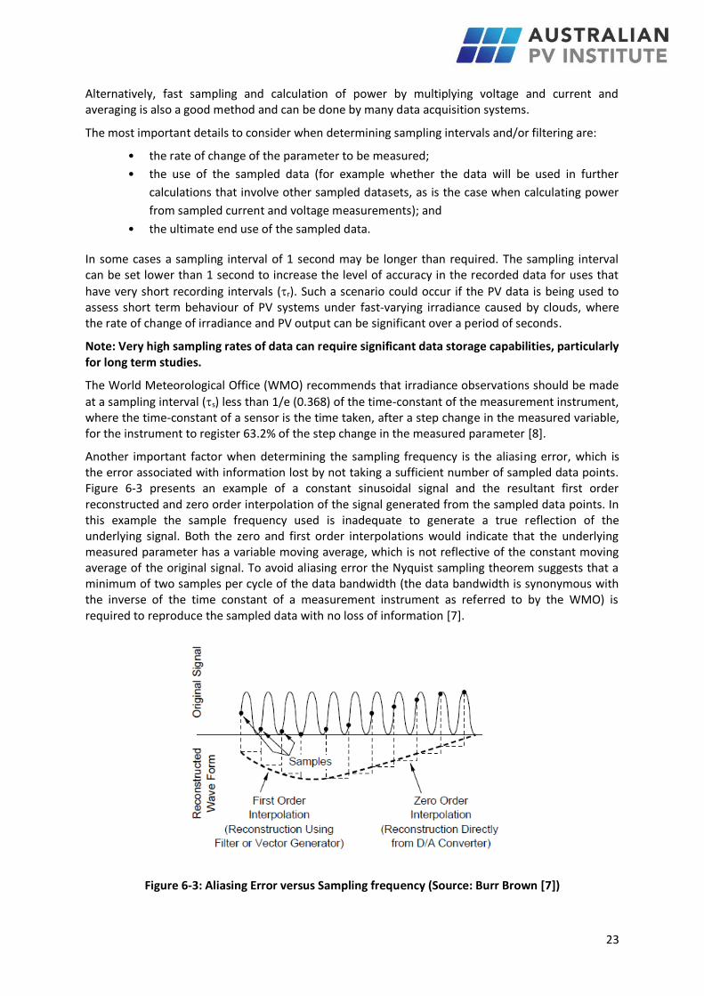
Another important factor when determining the sampling frequency is the aliasing error, which is the error associated with information lost by not taking a sufficient number of sampled data points. Figure 6-3 presents an example of a constant sinusoidal signal and the resultant first order reconstructed and zero order interpolation of the signal generated from the sampled data points. In this example the sample frequency used is inadequate to generate a true reflection of the underlying signal. Both the zero and first order interpolations would indicate that the underlying measured parameter has a variable moving average, which is not reflective of the constant moving average of the original signal. To avoid aliasing error the Nyquist sampling theorem suggests that a minimum of two samples per cycle of the data bandwidth (the data bandwidth is synonymous with the inverse of the time constant of a measurement instrument as referred to by the WMO) is required to reproduce the sampled data with no loss of information [7].

Figure 6-3: Aliasing Error versus Sampling frequency (Source: Burr Brown [7])

24

For example, the Nyquist theorem suggests that if the highest frequency in the signal to be sampled is fmax then the minimum sampling frequency would be 2fmax. However, this sampling frequency still does not achieve a very accurate reproduction of the original signal (average error between the reconstructed signal and the original signal is 32% at 2fmax) and an increase in the sampling frequency to 200fmax is required to achieve an accuracy of 1% in the reconstructed signal.

An alternative option is to filter the signal before sampling. This is a very effective method of reducing the maximum frequency of the signal, but filtering also results in the loss of information. This is not an issue if the ultimate use of the data is to calculate simple averages over a period of time. However if the data is to be used in a calculation involving other sampled parameters (for example the calculation of power from sampled voltage and current measurements) then analogue filtering before sampling removes fundamental elements of the time-dependent variation of the signal and may lead to the loss of accuracy in the calculated data. When determining the appropriate filtering level and sampling interval it is first necessary to consider the purpose for which the data is to be used and the rate at which the original signal may change.

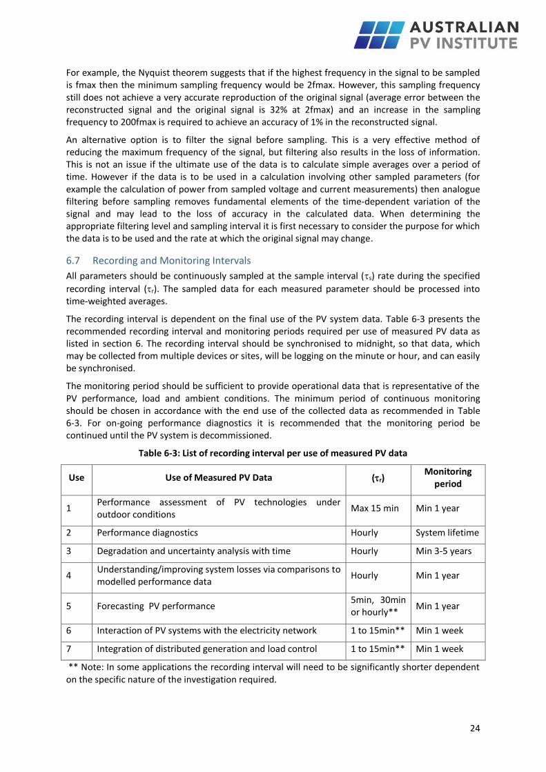
6.7 Recording and Monitoring Intervals

All parameters should be continuously sampled at the sample interval (s) rate during the specified

recording interval (r). The sampled data for each measured parameter should be processed into time-weighted averages.

The recording interval is dependent on the final use of the PV system data. Table 6-3 presents the recommended recording interval and monitoring periods required per use of measured PV data as listed in section 6. The recording interval should be synchronised to midnight, so that data, which may be collected from multiple devices or sites, will be logging on the minute or hour, and can easily be synchronised.

The monitoring period should be sufficient to provide operational data that is representative of the PV performance, load and ambient conditions. The minimum period of continuous monitoring should be chosen in accordance with the end use of the collected data as recommended in Table 6-3. For on-going performance diagnostics it is recommended that the monitoring period be continued until the PV system is decommissioned.

Table 6-3: List of recording interval per use of measured PV data


period






Hourly Min 1 year


Min 1 year




25

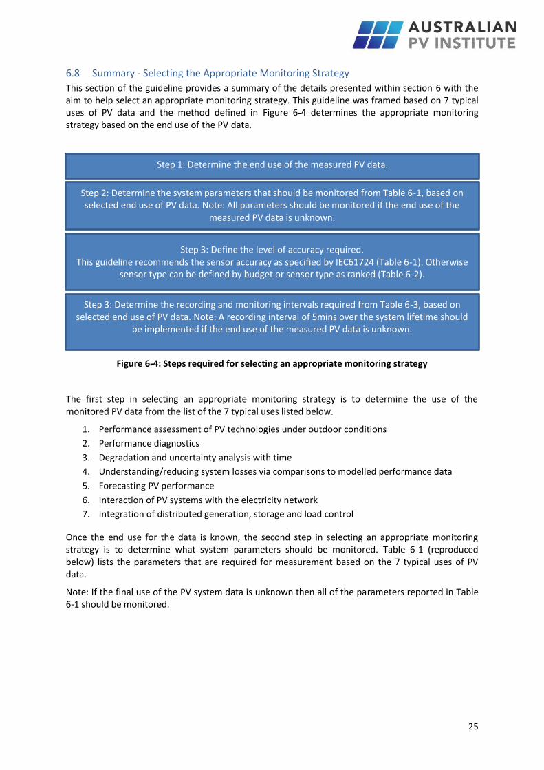
6.8 Summary - Selecting the Appropriate Monitoring Strategy

This section of the guideline provides a summary of the details presented within section 6 with the aim to help select an appropriate monitoring strategy. This guideline was framed based on 7 typical uses of PV data and the method defined in Figure 6-4 determines the appropriate monitoring strategy based on the end use of the PV data.

Figure 6-4: Steps required for selecting an appropriate monitoring strategy

The first step in selecting an appropriate monitoring strategy is to determine the use of the monitored PV data from the list of the 7 typical uses listed below.


2. Performance diagnostics




6. Interaction of PV systems with the electricity network


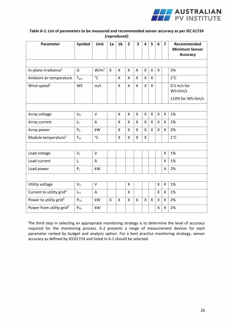
Once the end use for the data is known, the second step in selecting an appropriate monitoring strategy is to determine what system parameters should be monitored. Table 6-1 (reproduced below) lists the parameters that are required for measurement based on the 7 typical uses of PV data.

Note: If the final use of the PV system data is unknown then all of the parameters reported in Table 6-1 should be monitored.

Step 1: Determine the end use of the measured PV data.

Step 2: Determine the system parameters that should be monitored from Table 6-1, based on selected end use of PV data. Note: All parameters should be monitored if the end use of the

measured PV data is unknown.

Step 3: Define the level of accuracy required. This guideline recommends the sensor accuracy as specified by IEC61724 (Table 6-1). Otherwise

sensor type can be defined by budget or sensor type as ranked (Table 6-2).

Step 3: Determine the recording and monitoring intervals required from Table 6-3, based on selected end use of PV data. Note: A recording interval of 5mins over the system lifetime should

be implemented if the end use of the measured PV data is unknown.

26

Table 6-1: List of parameters to be measured and recommended sensor accuracy as per IEC 61724 (reproduced)

Parameter Symbol Unit 1a 1b 2 3 4 5 6 7 Recommended Minimum Sensor

Accuracy

In-plane irradiance1 G W/m2 X X X X X X X 5%

Ambient air temperature Tam °C X X X X X 1°C

Wind speed2 WS m/s X X X X X 0.5 m/s for WS<5m/s

±10% for WS>5m/s




Module temperature2 Tm °C X X X X 1°C





Current to utility grid4 ITU A X X X 1%

Power to utility grid4 PTU kW X X X X X X X X 2%

Power from utility grid4 PFU kW X X 2%

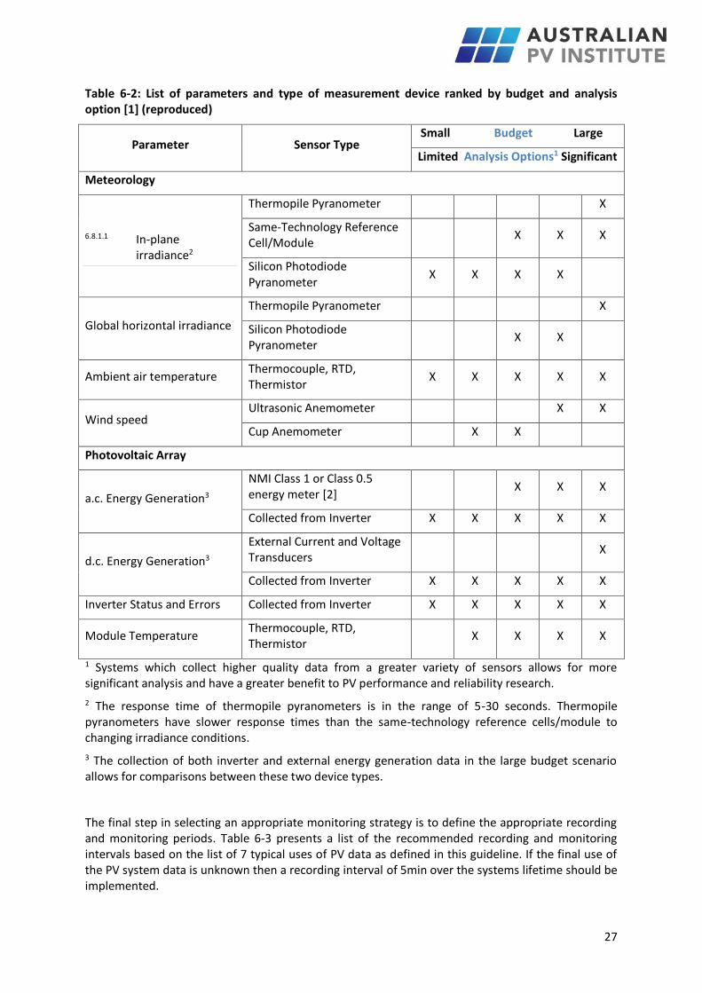
The third step in selecting an appropriate monitoring strategy is to determine the level of accuracy required for the monitoring process. 6-2 presents a range of measurement devices for each parameter ranked by budget and analysis option. For a best practice monitoring strategy, sensor accuracy as defined by IEC61724 and listed in 6-1 should be selected.

27

Table 6-2: List of parameters and type of measurement device ranked by budget and analysis option [1] (reproduced)



Meteorology

6.8.1.1 In-plane irradiance2



X X X


X X X X




X X


X X X X X


Cup Anemometer X X

Photovoltaic Array



X X X




X




X X X X


2 The response time of thermopile pyranometers is in the range of 5-30 seconds. Thermopile pyranometers have slower response times than the same-technology reference cells/module to changing irradiance conditions.


The final step in selecting an appropriate monitoring strategy is to define the appropriate recording and monitoring periods. Table 6-3 presents a list of the recommended recording and monitoring intervals based on the list of 7 typical uses of PV data as defined in this guideline. If the final use of the PV system data is unknown then a recording interval of 5min over the systems lifetime should be implemented.

28

Table 6-3: List of recording interval per use of measured PV data (reproduced)


period






Hourly Min 1 year


Min 1 year




29

7 Reliability Specifications

For measurement of system reliability a maintenance/monitoring log should be kept to record any of the following:

1. Scheduled and unscheduled maintenance

2. Unusual or extreme events such as weather events or grid outages

3. Component changes, failures or faults

4. Sensor issues, recalibration or change

5. Module and Sensor cleaning

6. Data acquisition system issues or changes

7. System operation issues or changes

8. Load issues or changes

All system maintenance must be explicitly documented. The maintenance/monitoring record should include dates and times for the start and end of each event. Table 7-1 presents an example of a maintenance log as recommended by the European Commission PV performance monitoring guidelines.

In addition, the following list identifies a number of items that should be visually inspected for on a regular basis and after extreme weather events. Any observations should be recorded in the maintenance/monitoring log.

1. PV modules –

1.1 Check for mechanical damage to glass or frame

1.2 Soiling

1.3 Delamination

1.4 Any visual changes i.e. colour, bubbles, uniformity or encapsulation, uniformity of surface

1.5 Any changes in shading from the external environment i.e. new buildings, tree growth

2. Mounting structure –

2.1 Check for mechanical damage or corrosion

2.2 Missing or loose connections/fixings

3. Electrical connections/earthing, cabling and junction boxes –

3.1 Inspect for damage by corrosion, wildlife etc.

3.2 Secure connections

3.3 Discolouration

3.4 Moisture ingress

3.5 Support of the cables and conduits

4. Inverter

4.1 Inspect external conditions i.e. damage to seals

4.2 Discolouration

4.3 Excessive noise

30

Table 7-1: Example maintenance record form (as taken from the European Commission PV performance guidelines [9])

Date and Time

Action3 Description of action

Person undertaking action

Material used4

Time taken for action

State of completion5

Counter readings6

Down time7 Comments and further action8

3 Action category: scheduled maintenance, fault inspection, fault diagnosis, repair 4 Material used: note any material or equipment used for repair or replacement, including serial numbers of old and new components if applicable 5 Stare of completion: indicate the state of completion of overall intervention resulting from this action 6 Counter readings: the energy counter reading (or equivalent measure of system output) should be recorded at the beginning and end of each action. This allows estimated of the amount of energy loss (if any) resulting from the cause of the intervention or the action itself 7 Down time: record any shutdowns of all or part of the system required to complete the action, including start time and period 8 Comments: any additional comments regarding the action and record all further actions required to complete the intervention, including schedule where possible.

31

8 Performance Assessment

This section of the guideline provides direction on how the recommended monitored data can be used to analyse PV system performance.

The extent to which losses and performance issues can be identified will be dependent on the accuracy of and uncertainty in of the measured data. The first step in the performance analysis is to check all recorded data for consistency and gaps to identify obvious anomalies in the dataset. The following procedure is based on the recommendations as presented in IEC 61724 and the European Commission PV performance guideline.

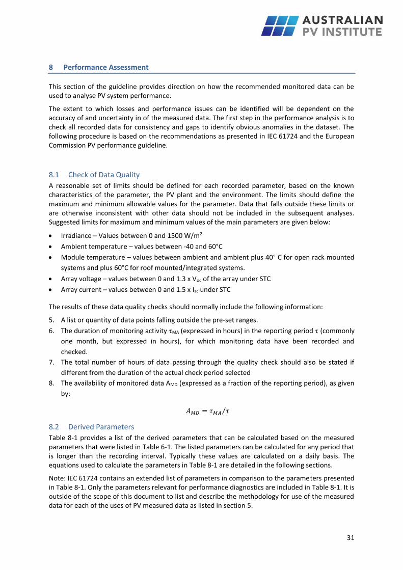
8.1 Check of Data Quality

A reasonable set of limits should be defined for each recorded parameter, based on the known characteristics of the parameter, the PV plant and the environment. The limits should define the maximum and minimum allowable values for the parameter. Data that falls outside these limits or are otherwise inconsistent with other data should not be included in the subsequent analyses. Suggested limits for maximum and minimum values of the main parameters are given below:

Irradiance – Values between 0 and 1500 W/m2

Ambient temperature – values between -40 and 60°C

Module temperature – values between ambient and ambient plus 40° C for open rack mounted

systems and plus 60°C for roof mounted/integrated systems.

Array voltage – values between 0 and 1.3 x Voc of the array under STC

Array current – values between 0 and 1.5 x Isc under STC

The results of these data quality checks should normally include the following information:

5. A list or quantity of data points falling outside the pre-set ranges.

6. The duration of monitoring activity MA (expressed in hours) in the reporting period (commonly

one month, but expressed in hours), for which monitoring data have been recorded and

checked.

7. The total number of hours of data passing through the quality check should also be stated if

different from the duration of the actual check period selected

8. The availability of monitored data AMD (expressed as a fraction of the reporting period), as given

by:

𝐴𝑀𝐷 = 𝜏𝑀𝐴 𝜏⁄

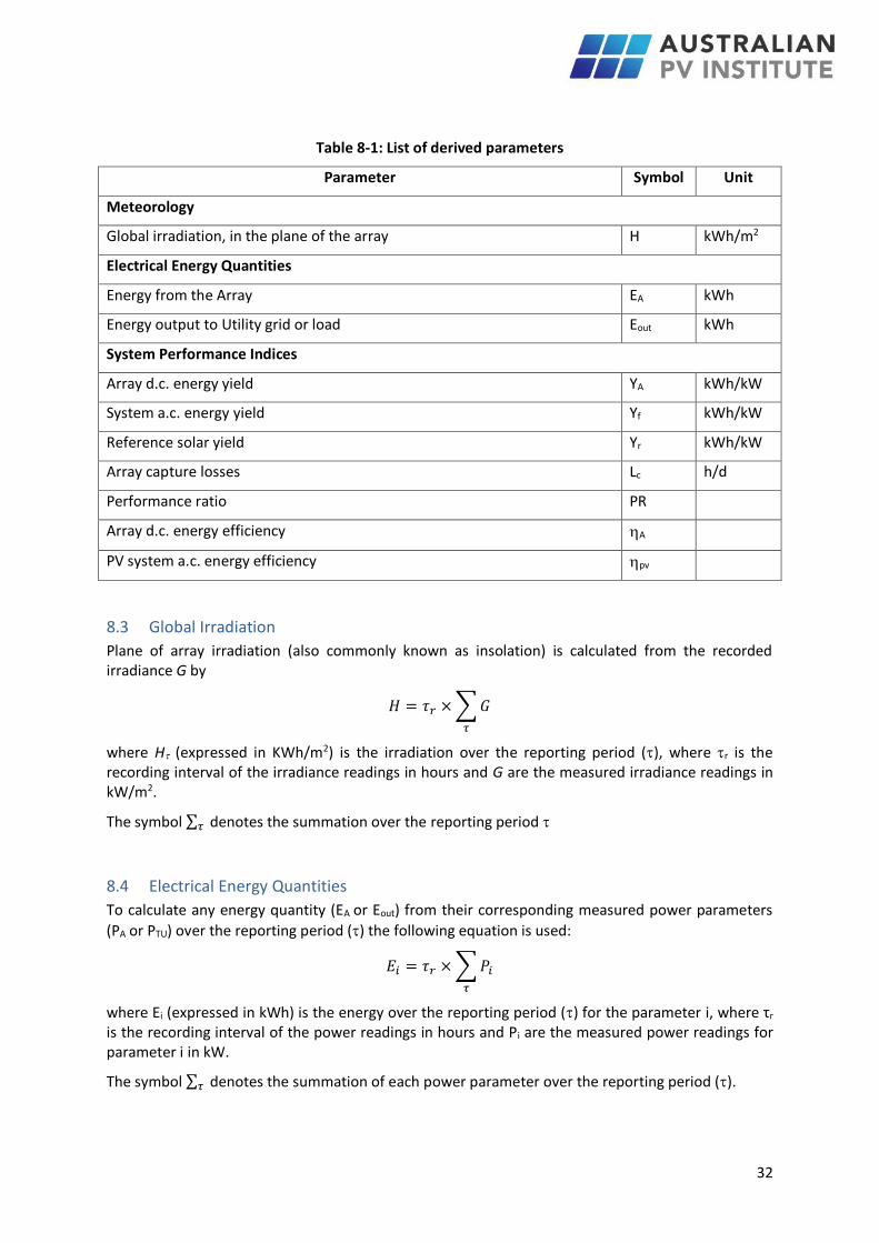
8.2 Derived Parameters

Table 8-1 provides a list of the derived parameters that can be calculated based on the measured parameters that were listed in Table 6-1. The listed parameters can be calculated for any period that is longer than the recording interval. Typically these values are calculated on a daily basis. The equations used to calculate the parameters in Table 8-1 are detailed in the following sections.

Note: IEC 61724 contains an extended list of parameters in comparison to the parameters presented in Table 8-1. Only the parameters relevant for performance diagnostics are included in Table 8-1. It is outside of the scope of this document to list and describe the methodology for use of the measured data for each of the uses of PV measured data as listed in section 5.

32

Table 8-1: List of derived parameters

Parameter Symbol Unit

Meteorology

Global irradiation, in the plane of the array H kWh/m2

Electrical Energy Quantities

Energy from the Array EA kWh

Energy output to Utility grid or load Eout kWh

System Performance Indices

Array d.c. energy yield YA kWh/kW

System a.c. energy yield Yf kWh/kW

Reference solar yield Yr kWh/kW

Array capture losses Lc h/d

Performance ratio PR

Array d.c. energy efficiency A

PV system a.c. energy efficiency pv

8.3 Global Irradiation

Plane of array irradiation (also commonly known as insolation) is calculated from the recorded irradiance G by

𝐻 = 𝜏𝑟 × ∑ 𝐺

𝜏

where H (expressed in KWh/m2) is the irradiation over the reporting period (), where r is the recording interval of the irradiance readings in hours and G are the measured irradiance readings in kW/m2.

The symbol ∑ 𝜏 denotes the summation over the reporting period

8.4 Electrical Energy Quantities

To calculate any energy quantity (EA or Eout) from their corresponding measured power parameters

(PA or PTU) over the reporting period () the following equation is used:

𝐸𝑖 = 𝜏𝑟 × ∑ 𝑃𝑖

𝜏

where Ei (expressed in kWh) is the energy over the reporting period () for the parameter i, where τr is the recording interval of the power readings in hours and Pi are the measured power readings for parameter i in kW.

The symbol ∑ 𝜏 denotes the summation of each power parameter over the reporting period ().

33

8.5 System Performance Indices

PV systems of different technologies, configurations and at different locations can be compared by calculating their normalised system performance indices such as yields, losses and efficiencies. Yields are energy quantities normalised to rated array power. System efficiencies are normalised to array area and losses are the differences between the yields. These parameters can be compared and tracked against parameters derived historically for the same system, allowing for identification of significant changes.

8.6 Yields

Yields are the ratios of energy quantities over the installed array’s rated output power P0 (kW). Yields indicate actual array operation relative to its rated capacity.

Note: Yields can be calculated over any time period. Daily, monthly and annual yields are the most frequently reported.

1. The array yield (YA) is the energy output of the PV array (EA) per kW of installed capacity.

𝑌𝐴 = 𝐸𝐴 𝑃0⁄

where P0 is the rated output power of the array under standard test conditions.

2. The final yield (Yf) is the net energy output of the entire PV system (Eout) expressed per

kWh/kW of installed capacity over the reporting period. The reporting period should be

recorded with the yield to avoid misinterpretation of the figures.

𝑌𝑓 = 𝐸𝑜𝑢𝑡 𝑃0⁄

3. The reference yield (Yr) can be calculated by dividing the total daily in-plane irradiation by

the module’s reference in-plane irradiance Gref (kW/m2), where Gref = 1kW/m2. For a

reporting interval of 24 hours, Yr is effectively the number of peak sun-hours (PSH)9 per day

(h/d).

𝑌𝑟 = 𝐻 𝐺𝑟𝑒𝑓⁄

8.6.1 Normalised Losses

Normalised losses can be calculated by finding the difference between reference, array and final yields. Two types of losses can be calculated once yields are determined. These are capture losses and system losses.

1) The array capture losses (Lc) represent the losses due to the array operating below what

would be expected at STC. Typical losses include the effect of temperature, high incidence

angles, shading, array circuit losses, including mismatch, low irradiance and soiling of the

array.

𝐿𝑐 = 𝑌𝑟 − 𝑌𝐴 Using these loss measures, maximum power point tracking (MPPT) losses will also appear as array capture losses, although they are not related to the array. However, in modern inverters, MPPT losses are generally very small. In most cases, inverter failures will also be counted as LC, since no power (or reduced power if limited) will be measured at the input to

9 PSH is the equivalent number of hours per day of irradiance of 1kW/m2 (the reference irradiance level) required to equal the actual irradiation.

34

the inverter. Care should be taken to prepare data for analysis in order to attribute losses appropriately.

2) The balance of system losses (LBOS) represent the losses that occur in the rest of the PV

system other than the array including losses due to wiring and the inverter.

𝐿𝐵𝑂𝑆 = 𝑌𝐴 − 𝑌𝑓

Note: No power will be measured at the input to the inverter, if a malfunction or inverter failure occurs. This will usually be reflected as a large LC, rather than LBOS. Unreliable inverters and complete system breakdowns appear statistically as high capture losses and relatively low system losses.

8.6.2 Performance Ratio

The performance ratio (PR), defined as the ratio of the final yield to the reference yield, indicates the overall effect of losses on the array’s rated output due to array temperature, incomplete utilisation of the irradiation and the system component inefficiencies or failures:

𝑃𝑅 = 𝑌𝑓/𝑌𝑟

PR is widely used for simple comparison of different grid-connected PV systems.

8.6.3 System Efficiencies

Efficiencies can be calculated for the whole system or for individual components within the system. In general efficiencies are the ratio of energy out to energy in represented as a percentage.

1) The array d.c. energy efficiency over the reporting period is defined by

𝜂𝐴 = 𝐸𝐴/(𝐴𝑎 × 𝐻)

where Aa is the active area of the array in m2.

This efficiency represents the average d.c. energy conversion efficiency of the PV array, which is

useful for comparison with the array efficiency A0 at its rated power, P0.

2) The PV system a.c. energy efficiency over the reporting period is defined by

𝜂𝑝𝑣 = 𝐸𝑜𝑢𝑡/(𝐴𝑎 × 𝐻)

Other efficiencies can also be calculated for example the inverter efficiency could be calculated as the a.c. energy output of the inverter to the d.c. power input into the inverter.

Note: The efficiency figures can be severely affected by poor BOS performance e.g. poor MPPT performance, by inverter failures or grid unavailability.

8.7 Identifying Performance Issues

This section of the guideline provides more details on the performance indices described previously, and provides a context for their use in identifying performance issues in PV systems, including when they are useful, and issues associated with their use. The information described in this section is based on information provided in [10, 11] and the European Commission’s performance monitoring guideline.

Reduction in system output caused by operational problems within the PV system will be reflected in the yields, efficiencies and ratios described earlier. The performance parameters can be compared against historically measured metrics for the same system or compared against predicted performance values. It should be noted however that each of these metrics has limitations in their

35

use due to the influence of weather on the calculated metric. For example the final PV system yield (Yf) is strongly influenced by its dependence on irradiance, so systems with a good solar resource will perform well on this measure. Yf essentially normalises the system performance with respect to system size so it is useful for comparing systems of different sizes and technologies to quantify the benefits of design components, or locations but it is not useful for identifying operational issues. Yf can only be used to identify issues within different sub-systems of the same array if separate monitoring of each sub-system has taken place.

The PR is typically used to diagnose system issues as it quantifies losses on the rated output of the PV system, and is influenced less by solar resource than Yf as it is normalised to solar radiation incident on the array (reference yield). It should, however, be noted that because the PR reflects losses due to module temperature, PR values tend to be greater in the winter than in the summer, and also for cold climates compared to hot climates. Other seasonal effects, like soiling, may also impact on the PR, where they vary significantly with the season. Decreasing yearly values of PR may be used to indicate a permanent loss in system performance, i.e. degradation in PV performance or worsening of shading problems. Large reductions in the PR indicate events that significantly impact the system performance, such as inverter failure or circuit breaker trips. Small or moderate decreases in PR can identify the existence of a problem, but not the cause. The European Commission guideline recommends that when the PR is less than 0.75, especially where a significant reduction in PR is observed in comparison with a previous period of similar operating conditions, then the reason for this reduction should be investigated. The approach is to consider the variation in the system output with time and/or irradiance level. This can most clearly be observed graphically.

The PV system a.c. -energy efficiency (PV) is a simple metric to calculate as it only requires the

measurement of in-plane irradiance and the a.c. power of the PV system. The advantage of the pv metric is that it provides a more accurate method for comparing the performance of widely different PV technologies as it is not dependent on the various reference conditions used to rate the different technologies [11].

8.7.1 Graphical Analysis

The following details a set of recommended graphical analyses that can be undertaken to help diagnose system performance issues when low PR values have been identified. This analysis has been taken from the European Commission’s Performance Monitoring Guidelines [9].

Note: It is worthwhile undertaking the following analysis on the sub-array data, if monitored, as issues on one or a section of the sub-arrays can be obscured when the total array output is plotted.

8.7.1.1 Clear Sky Day Analysis

For a clear sky day plot the a.c. output and in-plane irradiance as a function of time of day. If the a.c. output does not follow the same curve of the in-plane irradiance then the shape of the curve should be noted and compared to expected behaviour for different fault mechanisms.

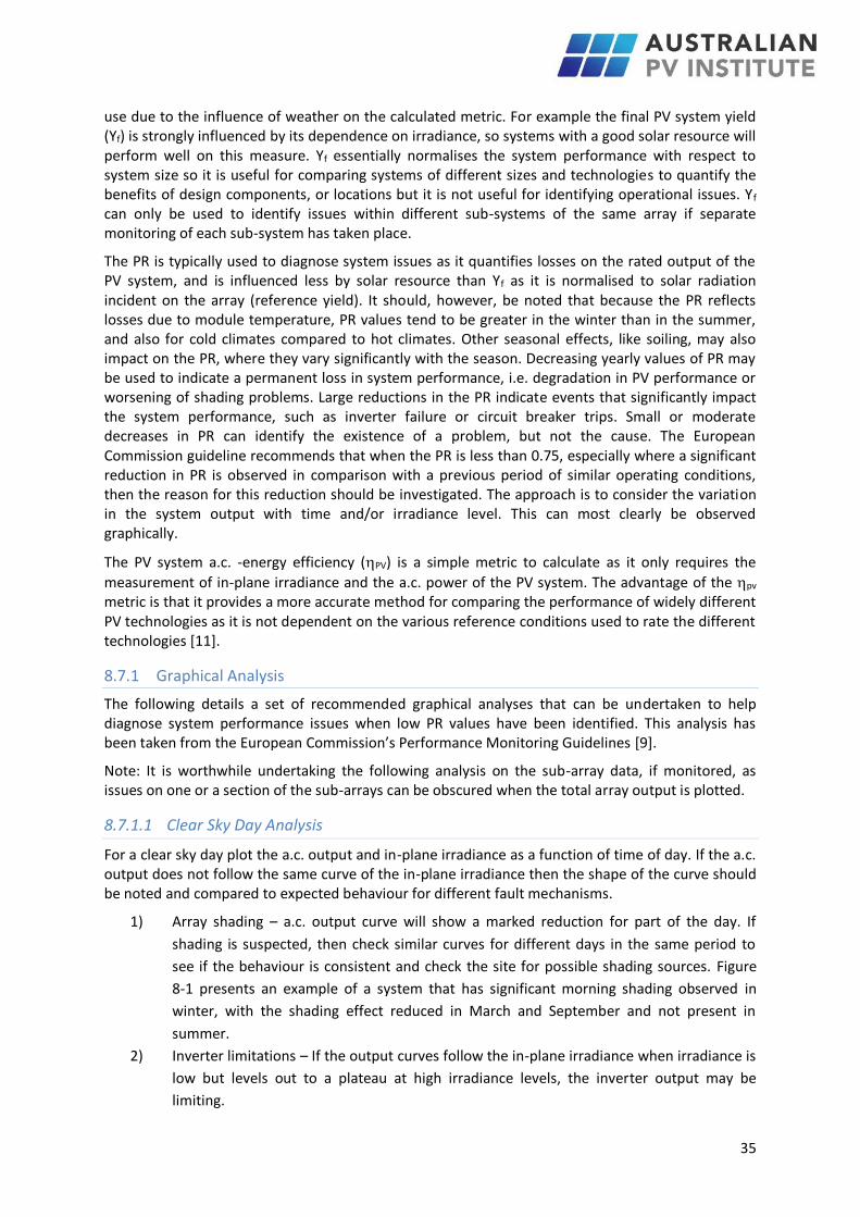
1) Array shading – a.c. output curve will show a marked reduction for part of the day. If

shading is suspected, then check similar curves for different days in the same period to

see if the behaviour is consistent and check the site for possible shading sources. Figure

8-1 presents an example of a system that has significant morning shading observed in

winter, with the shading effect reduced in March and September and not present in

summer.

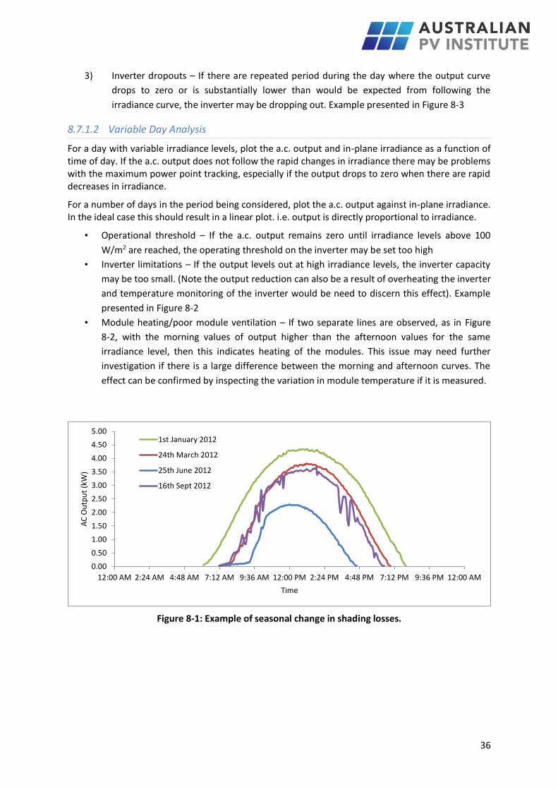
2) Inverter limitations – If the output curves follow the in-plane irradiance when irradiance is

low but levels out to a plateau at high irradiance levels, the inverter output may be

limiting.

36

3) Inverter dropouts – If there are repeated period during the day where the output curve

drops to zero or is substantially lower than would be expected from following the

irradiance curve, the inverter may be dropping out. Example presented in Figure 8-3

8.7.1.2 Variable Day Analysis

For a day with variable irradiance levels, plot the a.c. output and in-plane irradiance as a function of time of day. If the a.c. output does not follow the rapid changes in irradiance there may be problems with the maximum power point tracking, especially if the output drops to zero when there are rapid decreases in irradiance.

For a number of days in the period being considered, plot the a.c. output against in-plane irradiance. In the ideal case this should result in a linear plot. i.e. output is directly proportional to irradiance.

• Operational threshold – If the a.c. output remains zero until irradiance levels above 100

W/m2 are reached, the operating threshold on the inverter may be set too high

• Inverter limitations – If the output levels out at high irradiance levels, the inverter capacity

may be too small. (Note the output reduction can also be a result of overheating the inverter

and temperature monitoring of the inverter would be need to discern this effect). Example

presented in Figure 8-2

• Module heating/poor module ventilation – If two separate lines are observed, as in Figure

8-2, with the morning values of output higher than the afternoon values for the same

irradiance level, then this indicates heating of the modules. This issue may need further

investigation if there is a large difference between the morning and afternoon curves. The

effect can be confirmed by inspecting the variation in module temperature if it is measured.

Figure 8-1: Example of seasonal change in shading losses.

0.00

0.50

1.00

1.50

2.00

2.50

3.00

3.50

4.00

4.50

5.00

12:00 AM 2:24 AM 4:48 AM 7:12 AM 9:36 AM 12:00 PM 2:24 PM 4:48 PM 7:12 PM 9:36 PM 12:00 AM

AC

Ou

tpu

t (k

W)

Time

1st January 2012

24th March 2012

25th June 2012

16th Sept 2012

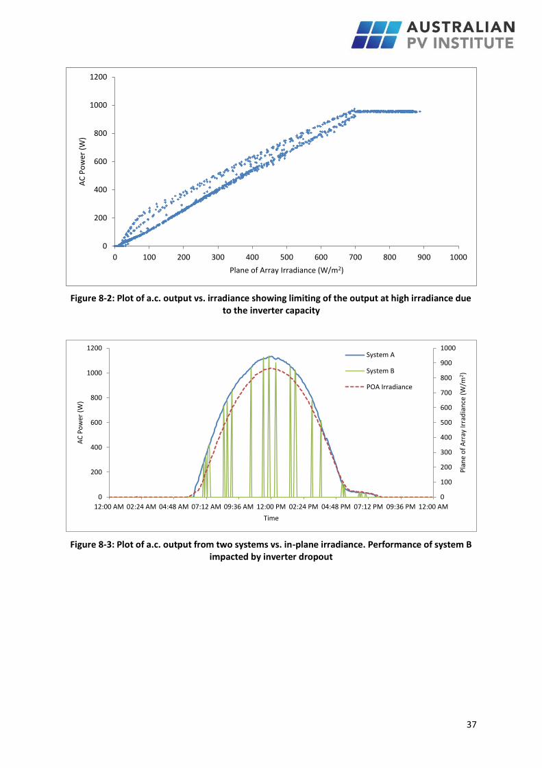
37

Figure 8-2: Plot of a.c. output vs. irradiance showing limiting of the output at high irradiance due to the inverter capacity

Figure 8-3: Plot of a.c. output from two systems vs. in-plane irradiance. Performance of system B impacted by inverter dropout

0

200

400

600

800

1000

1200

0 100 200 300 400 500 600 700 800 900 1000

AC

Po

wer

(W

)

Plane of Array Irradiance (W/m2)

0

100

200

300

400

500

600

700

800

900

1000

0

200

400

600

800

1000

1200

12:00 AM 02:24 AM 04:48 AM 07:12 AM 09:36 AM 12:00 PM 02:24 PM 04:48 PM 07:12 PM 09:36 PM 12:00 AM

Pla

ne

of

Arr

ay Ir

rad

ian

ce (

W/m

2 )

AC

Po

wer

(W

)

Time

System A

System B

POA Irradiance

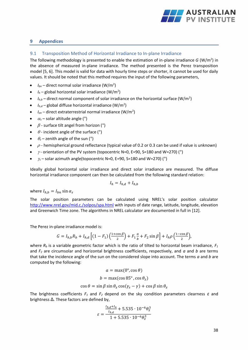
38

9 Appendices

9.1 Transposition Method of Horizontal Irradiance to In-plane Irradiance

The following methodology is presented to enable the estimation of in-plane irradiance G (W/m2) in the absence of measured in-plane irradiance. The method presented is the Perez transposition model [5, 6]. This model is valid for data with hourly time steps or shorter, it cannot be used for daily values. It should be noted that this method requires the input of the following parameters,

Ibn – direct normal solar irradiance (W/m2)

Ih – global horizontal solar irradiance (W/m2)

Ih,b – direct normal component of solar irradiance on the horizontal surface (W/m2)

Ih,d – global diffuse horizontal irradiance (W/m2)

Ion – direct extraterrestrial normal irradiance (W/m2)

s – solar altitude angle (°)

- surface tilt angel from horizon (°)

- incident angle of the surface (°)

z – zenith angle of the sun (°)

- hemispherical ground reflectance (typical value of 0.2 or 0.3 can be used if value is unknown)

- orientation of the PV system (topocentric N=0, E=90, S=180 and W=270) (°)

s – solar azimuth angle(topocentric N=0, E=90, S=180 and W=270) (°)

Ideally global horizontal solar irradiance and direct solar irradiance are measured. The diffuse horizontal irradiance component can then be calculated from the following standard relation:

𝐼ℎ = 𝐼ℎ,𝑑 + 𝐼ℎ,𝑏

where 𝐼ℎ,𝑏 = 𝐼𝑏𝑛 sin 𝛼𝑠

The solar position parameters can be calculated using NREL’s solar position calculator http://www.nrel.gov/mid.c./solpos/spa.html with inputs of date range, latitude, longitude, elevation and Greenwich Time zone. The algorithms in NREL calculator are documented in full in [12].

The Perez in-plane irradiance model is:

𝐺 = 𝐼ℎ,𝑏𝑅𝑏 + 𝐼ℎ,𝑑 [(1 − 𝐹1) (1+cos 𝛽

2) + 𝐹1

𝑎

𝑏+ 𝐹2 sin 𝛽] + 𝐼ℎ𝜌 (

1−cos 𝛽

2),

where Rb is a variable geometric factor which is the ratio of tilted to horizontal beam irradiance, F1 and F2 are circumsolar and horizontal brightness coefficients, respectively, and a and b are terms that take the incidence angle of the sun on the considered slope into account. The terms a and b are computed by the following:

𝑎 = max (0°, cos 𝜃)

𝑏 = max (cos 85° , cos 𝜃𝑧)

cos 𝜃 = sin 𝛽 sin 𝜃𝑧 cos(𝛾𝑠 − 𝛾) + cos 𝛽 sin 𝜃𝑧

The brightness coefficients F1 and F2 depend on the sky condition parameters clearness ε and brightness Δ. These factors are defined by,

𝜀 =

𝐼ℎ,𝑑+𝐼𝑛

𝐼ℎ,𝑑+ 5.535 ∙ 10−6𝜃𝑧

3

1 + 5.535 ∙ 10−6𝜃𝑧3

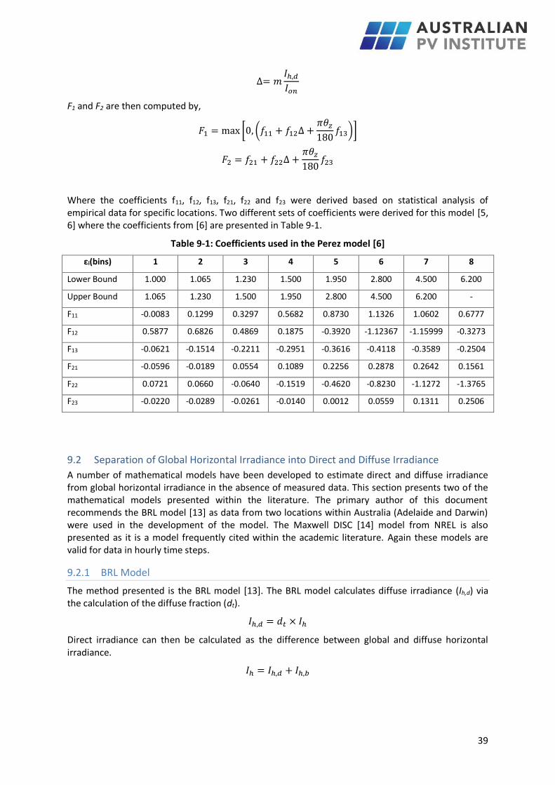
http://www.nrel.gov/midc/solpos/spa.html

39

∆= 𝑚𝐼ℎ,𝑑

𝐼𝑜𝑛

F1 and F2 are then computed by,

𝐹1 = max [0, (𝑓11 + 𝑓12∆ +𝜋𝜃𝑧

180𝑓13)]

𝐹2 = 𝑓21 + 𝑓22∆ +𝜋𝜃𝑧

180𝑓23

Where the coefficients f11, f12, f13, f21, f22 and f23 were derived based on statistical analysis of empirical data for specific locations. Two different sets of coefficients were derived for this model [5, 6] where the coefficients from [6] are presented in Table 9-1.

Table 9-1: Coefficients used in the Perez model [6]

εi(bins) 1 2 3 4 5 6 7 8

Lower Bound 1.000 1.065 1.230 1.500 1.950 2.800 4.500 6.200

Upper Bound 1.065 1.230 1.500 1.950 2.800 4.500 6.200 -

F11 -0.0083 0.1299 0.3297 0.5682 0.8730 1.1326 1.0602 0.6777

F12 0.5877 0.6826 0.4869 0.1875 -0.3920 -1.12367 -1.15999 -0.3273

F13 -0.0621 -0.1514 -0.2211 -0.2951 -0.3616 -0.4118 -0.3589 -0.2504

F21 -0.0596 -0.0189 0.0554 0.1089 0.2256 0.2878 0.2642 0.1561

F22 0.0721 0.0660 -0.0640 -0.1519 -0.4620 -0.8230 -1.1272 -1.3765

F23 -0.0220 -0.0289 -0.0261 -0.0140 0.0012 0.0559 0.1311 0.2506

9.2 Separation of Global Horizontal Irradiance into Direct and Diffuse Irradiance

A number of mathematical models have been developed to estimate direct and diffuse irradiance from global horizontal irradiance in the absence of measured data. This section presents two of the mathematical models presented within the literature. The primary author of this document recommends the BRL model [13] as data from two locations within Australia (Adelaide and Darwin) were used in the development of the model. The Maxwell DISC [14] model from NREL is also presented as it is a model frequently cited within the academic literature. Again these models are valid for data in hourly time steps.

9.2.1 BRL Model

The method presented is the BRL model [13]. The BRL model calculates diffuse irradiance (Ih,d) via the calculation of the diffuse fraction (dt).

𝐼ℎ,𝑑 = 𝑑𝑡 × 𝐼ℎ

Direct irradiance can then be calculated as the difference between global and diffuse horizontal irradiance.

𝐼ℎ = 𝐼ℎ,𝑑 + 𝐼ℎ,𝑏

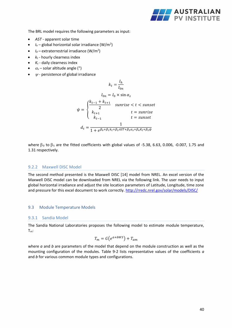
40

The BRL model requires the following parameters as input:

AST - apparent solar time

Ih – global horizontal solar irradiance (W/m2)

I0 – extraterrestrial irradiance (W/m2)

kt - hourly clearness index

Kt - daily clearness index

s – solar altitude angle (°)

- persistence of global irradiance

𝑘𝑡 =𝐼ℎ

𝐼0𝑛

𝐼0𝑛 = 𝐼0 × sin 𝛼𝑠

𝜓 = {

𝑘𝑡−1 + 𝑘𝑡+1

2 𝑠𝑢𝑛𝑟𝑖𝑠𝑒 < 𝑡 < 𝑠𝑢𝑛𝑠𝑒𝑡

𝑘𝑡+1 𝑡 = 𝑠𝑢𝑛𝑟𝑖𝑠𝑒𝑘𝑡−1 𝑡 = 𝑠𝑢𝑛𝑠𝑒𝑡

𝑑𝑡 =1

1 + 𝑒𝛽0+𝛽1𝑘𝑡+𝛽2𝐴𝑆𝑇+𝛽3𝛼𝑠+𝛽4𝐾𝑡+𝛽5𝜓

where 0 to 5 are the fitted coefficients with global values of -5.38, 6.63, 0.006, -0.007, 1.75 and 1.31 respectively.

9.2.2 Maxwell DISC Model

The second method presented is the Maxwell DISC [14] model from NREL. An excel version of the Maxwell DISC model can be downloaded from NREL via the following link. The user needs to input global horizontal irradiance and adjust the site location parameters of Latitude, Longitude, time zone and pressure for this excel document to work correctly. http://rredc.nrel.gov/solar/models/DISC/

9.3 Module Temperature Models

9.3.1 Sandia Model

The Sandia National Laboratories proposes the following model to estimate module temperature, Tm:

𝑇𝑚 = 𝐺(𝑒𝑎+𝑏𝑊𝑆) + 𝑇𝑎𝑚

where a and b are parameters of the model that depend on the module construction as well as the mounting configuration of the modules. Table 9-2 lists representative values of the coefficients a and b for various common module types and configurations.

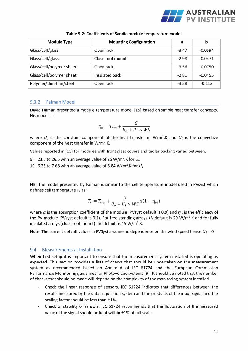
http://rredc.nrel.gov/solar/models/DISC/

41

Table 9-2: Coefficients of Sandia module temperature model

Module Type Mounting Configuration a b

Glass/cell/glass Open rack -3.47 -0.0594

Glass/cell/glass Close roof mount -2.98 -0.0471

Glass/cell/polymer sheet Open rack -3.56 -0.0750

Glass/cell/polymer sheet Insulated back -2.81 -0.0455

Polymer/thin-film/steel Open rack -3.58 -0.113

9.3.2 Faiman Model

David Faiman presented a module temperature model [15] based on simple heat transfer concepts. His model is:

𝑇𝑚 = 𝑇𝑎𝑚 +𝐺

𝑈𝑜 + 𝑈1 × 𝑊𝑆

where Uo is the constant component of the heat transfer in W/m2.K and U1 is the convective component of the heat transfer in W/m2.K.

Values reported in [15] for modules with front glass covers and tedlar backing varied between:

9. 23.5 to 26.5 with an average value of 25 W/m2.K for Uo

10. 6.25 to 7.68 with an average value of 6.84 W/m2.K for U1

NB: The model presented by Faiman is similar to the cell temperature model used in PVsyst which defines cell temperature Tc as:

𝑇𝑐 = 𝑇𝑎𝑚 +𝐺

𝑈𝑜 + 𝑈1 × 𝑊𝑆𝛼(1 − ƞ𝑚)

where is the absorption coefficient of the module (PVsyst default is 0.9) and ƞm is the efficiency of the PV module (PVsyst default is 0.1). For free standing arrays Uo default is 29 W/m2.K and for fully insulated arrays (close roof mount) the default is 15 W/m2.K.

Note: The current default values in PVSyst assume no dependence on the wind speed hence U1 = 0.

9.4 Measurements at Installation

When first setup it is important to ensure that the measurement system installed is operating as expected. This section provides a lists of checks that should be undertaken on the measurement system as recommended based on Annex A of IEC 61724 and the European Commission Performance Monitoring guidelines for Photovoltaic systems [9]. It should be noted that the number of checks that should be made will depend on the complexity of the monitoring system installed.

- Check the linear response of sensors. IEC 61724 indicates that differences between the

results measured by the data acquisition system and the products of the input signal and the

scaling factor should be less than ±1%.

- Check of stability of sensors. IEC 61724 recommends that the fluctuation of the measured

value of the signal should be kept within ±1% of full scale.

42

- Check all channels are recording correctly and investigate the reasons for any missing data

- Check that data values are within an appropriate range for the parameter being measured

as per section 8.1.

- If any parameters are not within the correct range:

o Check any calculations that are made to determine the logged values are correctly

implemented

o Check the operation connections and positioning of the sensor

o Check for electromagnetic noise disrupting the signal form the sensor (Note: this

would often be expected to affect more than one sensor)

The European Commission performance monitoring guidelines recommends the following analyses should be undertaken over a period of time at the beginning of operation of the system to determine the typical performance of the PV system and to identify any major losses existing at installation.

9.4.1 Analysis 1 – Clear Day Analysis

The aim of this analysis is to determine the typical output of the PV system under high irradiance conditions.

On a clear, sunny day, measure the energy output, the solar irradiation and the average ambient temperature and calculate final yield, system efficiency and performance ratio for the day. Record all values and keep as a record. Verify that the performance parameters are within the expected range. If the parameters fall outside the expected range, follow the instructions in section 8.7 to identify the cause of the issue.

9.4.2 Analysis 2 – Variation of Output across a Typical Day

The aim of this analysis is to determine the expected level of variation of the system performance across a typical sunny day.

On a clear, sunny day, record the energy output and solar irradiation at the recording interval that is to be used for long term monitoring (i.e. the first use of PV data as listed in section 0). On the same graph plot both quantities against time and follow the procedure detailed in section 8.7 to identify whether any performance issues exist. Record all values and the analysis and keep as a record.

9.4.3 Analysis 3 – Other Days Analysis

The aim of this analysis is to determine the typical output of the PV system under a range of possible weather scenarios.

Repeat Analysis 1 for a number of days where each day has a different weather profile. Ideally include days with a range of irradiation levels and ambient temperature conditions. Record all values and keep as a record. Verify that the performance parameters are reasonable given the weather conditions for that day.

Note: The range of levels and weather scenarios possible will depend on the prevailing climate at the location and the time of year the initial analysis is undertaken. Date of the analysis should be included in all the analysis records.

9.4.4 Analysis 4 – Inverter Measurements

The aim of this analysis is to determine the expected behaviour of the inverter under different operating conditions.

43

Performance data, both on the d.c. input side and a.c. output side of the inverter, should be measured and kept on record for each of the following scenarios. A minimum test period of 200ms is recommended to avoid system instability/disturbance.

Conditions of zero solar irradiance in order to get information on self-consumption in

idling conditions and at night time.

With increasing solar radiation the variation in voltage and current on the d.c. side and

the a.c. power flow in both directions should be monitored for the moment at which the

inverter starts full operation. Repeat test over a day to detect inverter/MPPT start-up

and shut-down thresholds

In the course of the day several measurements should be done at a range of power

levels.

If the inverter is rated lower than the PV array, establish the reaction to overload if

irradiance permits.

With inverter connected to the grid, monitor for current harmonics.

If possible, disconnect inverter and measure grid current, voltage and harmonics.

With the inverter connected to the grid, disconnect the array and measure a.c. power

backflow into the inverter (check if inverter is in a ‘night-time’ or ‘standby’ mode).

During operation the inverter should be switched off and on in order to get information

on the starting procedure after shut down.

The starting procedure should also be tested by switching off and on the grid when the

inverter is under normal operation.

44

10 References

1. Emery, K. and R. Smith, Monitoring System Performance. PV Module Reliability Workshop, NREL/PR-5200-50643, February 16, 2011.

2. NMI, NMI M 6-1 Electricity Meters Part 1: Metrological and Technical Requirements. Australian Government National Measurement Institute, 2012.

3. Sengupta, M., P. Gotseff, and T. Stoffel, Evaluation of Photodiode and Thermopile Pyranometers for Photovoltaic Applications. 27th EUPVSEC, Frankfurt, Germany, 2012: p. 3705-3708.

4. Reinhardt, S., et al., Influence of Technology Differences in Performance Ratio Calculations. 27th EUPVSEC, Frankfurt, Germany, 2012: p. 4025-4026.

5. Perez, R., et al., A new simplified version of the Perez diffuse irradiance model for tilted surfaces. Solar Energy, 1987. 36(6): p. 481-497.

6. Perez, R., P. Ineichen, and R. Seals, Modelling daylight availability and irradiance components from direct and global irradiance. Solar Energy, 1990. 44: p. 271-289.

7. Brown, B., Application Bulletin: Principles of Data Acquisition and Conversion. Texas Instrument Incorporated, http://www.ti.com/lit/an/sbaa051/sbaa051.pdf, 2000. Accessed: 20/05/2013.

8. WMO, Guide to Meteorological Instruments and Methods of Observation: (CIMO guide). World Meteorological Organisation, 2012. No. 8.

9. PERFORMANCE, Monitoring Guidelines for Photovoltaic Systems. PERFORMANCE project funded by the European Commission 6th Framework Programme, Contract No: SES-019718. http://re.jrc.ec.europa.eu/monitoring/monitoring_main.php.

10. Marion, B., et al. NREL/CP-520-37358: Performance Parameters for Grid-Connected PV Systems. in 31st IEEE Photovoltaics Specialists Conference and Exhibtion. 2005. Florida, January 3-7.

11. King, D.L. More "efficient" methods for specifying and monitoring PV system performance. in Photovoltaic Specialists Conference (PVSC), 2011 37th IEEE. 2011.

12. Reda, I. and A. Andreas, Solar Position Algorithm for Solar Radiation Applications. NREL/TP-560-34302, Golden Colorado, http://www.nrel.gov/docs/fy08osti/34302.pdf, 2008.

13. Ridley, B., J. Boland, and P. Lauret, Modelling of diffuse solar fraction with multiple predictors. Renewable Energy, 2010. 35(2): p. 478-483.

14. Maxwell, E., A quasi physical model for converting hourly global horizontal to direct normal insolation. SERI/TR-215-3087. Golden, Colorado: Solar Energy Research Institute, 1987.

15. Faiman, D., Assessing the outdoor operating temperature of photovolatic modules. Progress in Photovoltaics, 2008. 16(4): p. 307-315.

http://www.ti.com/lit/an/sbaa051/sbaa051.pdf

http://re.jrc.ec.europa.eu/monitoring/monitoring_main.php

http://www.nrel.gov/docs/fy08osti/34302.pdf

Documents

Australian Technical Guidelines for Monitoring and ...apvi.org.au/wp-content/uploads/2013/11/Australian... · Australian Technical Guidelines for Monitoring and Analysing Photovoltaic