Embed Size (px)
Citation preview

This article appeared in a journal published by Elsevier. The attachedcopy is furnished to the author for internal non-commercial researchand education use, including for instruction at the authors institution
and sharing with colleagues.
Other uses, including reproduction and distribution, or selling orlicensing copies, or posting to personal, institutional or third party
websites are prohibited.
In most cases authors are permitted to post their version of thearticle (e.g. in Word or Tex form) to their personal website orinstitutional repository. Authors requiring further information
regarding Elsevier’s archiving and manuscript policies areencouraged to visit:
http://www.elsevier.com/copyright
Author's personal copy
J. Differential Equations 251 (2011) 1276–1304
Contents lists available at ScienceDirect
Journal of Differential Equations
www.elsevier.com/locate/jde
Dynamics and pattern formation in a diffusivepredator–prey system with strong Allee effect in prey ✩
Jinfeng Wang a,b, Junping Shi c,∗, Junjie Wei b
a School of Mathematics and Y.Y. Tseng Functional Analysis Research Center, Harbin Normal University, Harbin, Heilongjiang, 150025,PR Chinab Department of Mathematics, Harbin Institute of Technology, Harbin, Heilongjiang, 150001, PR Chinac Department of Mathematics, College of William and Mary, Williamsburg, VA 23187-8795, USA
a r t i c l e i n f o a b s t r a c t
Article history:Received 3 November 2010Revised 4 March 2011Available online 24 March 2011
MSC:35K5735B3635B3292D40
Keywords:Reaction–diffusion systemPredator–preyBifurcationStrong Allee effectSpatiotemporal patterns
The dynamics of a reaction–diffusion predator–prey system withstrong Allee effect in the prey population is considered. Nonexis-tence of nonconstant positive steady state solutions are shown toidentify the ranges of parameters of spatial pattern formation. Bi-furcations of spatially homogeneous and nonhomogeneous periodicsolutions as well as nonconstant steady state solutions are studied.These results show that the impact of the Allee effect essentiallyincreases the system spatiotemporal complexity.
© 2011 Elsevier Inc. All rights reserved.
1. Introduction
The understanding of patterns and mechanisms of spatial dispersal of interacting species is an is-sue of significant current interest in conservation biology and ecology, and biochemical reactions.Different species of chemical or living organisms compete and/or consume limited resource, andsuch competition and consumption also generate feedbacks in the complex network of biological
✩ This research is partially supported by the National Natural Science Foundation of China (Nos. 11031002, 11071051),National Science Foundation of US (DMS-1022648).
* Corresponding author.E-mail addresses: [email protected] (J. Wang), [email protected] (J. Shi), [email protected] (J. Wei).
0022-0396/$ – see front matter © 2011 Elsevier Inc. All rights reserved.doi:10.1016/j.jde.2011.03.004
Author's personal copy
J. Wang et al. / J. Differential Equations 251 (2011) 1276–1304 1277
species. The spatial dispersal makes the dynamics and behavior of the organisms even more com-plicated. A typical type of interaction is the one between a pair of predator and prey, or moregenerally, a pair of consumer and resource. Mathematical model of predator–prey type has playeda major role in the studies of biological invasion of foreign species, epidemics spreading, extinc-tion/spread of flame balls in combustion or autocatalytic chemical reaction. A variety of theoreticalapproaches has been developed and considerable progress has been made during the last threedecades [5,8,11,26,30,35,44].
The spatiotemporal dynamics of a predator–prey system in a homogeneous environment can bedescribed by a system of nonlinear parabolic partial differential equations (or reaction–diffusion equa-tions) [26,33–35,40]:
∂ H(X, T )
∂T= D1�H + F (H)H − G(H)P ,
∂ P (X, T )
∂T= D2�P + kG(H)P − M(P ), (1.1)
where H(X, T ) and P (X, T ) are the densities of prey and predator at time T and position X respec-tively; here X ∈ ΩO (⊆ Rn) is the spatial habitat of the two species; the Laplace operator � describesthe spatial dispersal with passive diffusion; D1 and D2 are the diffusion coefficients of species andk is the food utilization coefficient. The function F (H) describes the per capita growth rate of theprey, G(H) is the functional response of the predator, which corresponds to the saturation of theirappetites and reproductive capacity, and M(P ) stands for predator mortality.
The functions F (H), G(H) and M(P ) can be of different types in various specific situations. Sincethe first differential equation model of predator–prey type Lotka–Volterra equation was formulated[27,52] in 1920s, a logistic type growth F (H) is usually assumed for the prey species in the models,while a linear mortality rate M(P ) is assumed for the predator. Some conventional functional responsefunctions G(H) include Holling types I, II, III and Ivlev type (see [17,24,43,53]). When F (H) is of alogistic growth, the dynamics of (1.1) has been considered in many articles, see for example [11,13,19,25,28,60].
In recent years, Allee effect in the growth of a population has been studied extensively [9]. Alleeeffect is named after ecologist Warder C. Allee [2]. A strong Allee effect refers to the phenomenonthat the population has a negative growth when the size of the population is below certain thresholdvalue [3,47,50,53], while a weak Allee effect means that growth is positive and increasing when belowa threshold [22,47,56].
By means of extensive computer simulations, Lewis and Karevia [26] used a scalar partial dif-ferential equation to model the population and they found that strong Allee effect may reduce thespread of invading organisms; Owen and Lewis [35] considered (1.1) and indicated that predationpressure can slow, stop or reverse a spatial invasion of prey; Morozov, Petrovskii and Li [32,33,39,40]showed that the dynamic of system (1.1) is remarkably rich and that its complexity increases withan increase of the prey maximum growth rate; Also in [33], a thorough study of the system (1.1) inconnection to biological invasion is fulfilled and a detailed classification of possible patterns of speciesspread and even the spatiotemporal chaos are obtained. Note that most of these studies are numericalnot analytical. There are very little mathematical analysis results for (1.1) with strong Allee effect inprey.
On the other hand, the authors [53,54] have recently completed a comprehensive study of a gen-eral ODE predator–prey system with strong Allee effect in prey. In [53] we considered a planar ODEsystem
⎧⎪⎪⎨⎪⎪⎩du
dt= g(u)
(f (u) − v
),
dv
dt= v
(g(u) − d
),
(1.2)
Author's personal copy
1278 J. Wang et al. / J. Differential Equations 251 (2011) 1276–1304
where g(u) is the predator functional response which an increasing function, and f (u) is a functionwith strong Allee effect character. We completely classified the global dynamics of (1.2) when f andg satisfy some mild conditions. In particular, we showed that the dynamics is mostly bistable withone stable state (0,0) and the other one being an equilibrium, or a periodic orbit, or a loop of hete-roclinic orbits for a threshold parameter value, and in the other case, (0,0) is globally asymptoticallystable.
In this paper, we rigorously consider the dynamics of the system (1.1) with the form considered in[32,33,40]. That is, we assume that the functional response is of Holling type II [17], and the predatormortality rate is linear:
G(H) = AH
H + B, M(P ) = M P ,
where A describes the maximum predation rate, B is the self-saturation prey density and M is theper capita mortality rate; and the prey growth rate is given by the form in [26]:
F (H) = 4ω
(K − H0)2H(H − H0)(K − H),
where K is the prey carrying capacity, ω is the maximum per capita growth rate and H0 quantifiesthe intensity of the Allee effect so that it is strong with 0 < H0 < K .
With these choices of functions and using new dimensionless variables and parameters:
u = H
K, v = P
kK, γ = 4ω
(K − H0)2, t = γ H0T
K 2, l = AKk
B, x = √
lX,
we consider the following nondimensionalized form of reaction–diffusion model:⎧⎪⎪⎪⎪⎪⎪⎪⎪⎨⎪⎪⎪⎪⎪⎪⎪⎪⎩
∂u
∂t= d1�u + u(1 − u)
(u
b− 1
)− muv
a + u, x ∈ Ω, t > 0,
∂v
∂t= d2�v − dv + muv
a + u, x ∈ Ω, t > 0,
∂u
∂n= ∂v
∂n= 0, x ∈ ∂Ω, t > 0,
u(x,0) = u0(x) � 0, v(x,0) = v0(x) � 0, x ∈ Ω,
(1.3)
where the new parameters are
d1 = D1lK 2
H0γ, d2 = D2lK 2
H0γ, m = AK 2k
γ H0, d = M K 3kl
γ H0, a = B
K, b = H0
K.
For the new parameters, d is the death rate of the predator, a measures the saturation effect [17]and m is the strength of the interaction. The Allee threshold is b = H0/K < 1 [3,51,56]: a strong Alleeeffect introduces a population threshold, and the population must surpass this threshold to grow. Weconsider an initial–boundary value problem over a smooth bounded spatial domain Ω ⊂ Rn for n � 1,and we impose a no-flux boundary condition so it is a closed ecosystem.
In this paper we prove the global existence of the solutions to (1.3), and in various situations,global asymptotical behavior of the solutions can be determined. In particular, we show that a largeamount of predator initially will always drive both population into extinction, which is called overex-ploitation [51,53] and it is a character of predator–prey system with Allee effect. We also use energyestimates to obtain a priori bounds of the dynamic and steady state solutions, which also identifiesthe regions of parameters of nonexistence of nonconstant spatial patterns. While a precise description
Author's personal copy
J. Wang et al. / J. Differential Equations 251 (2011) 1276–1304 1279
of the global dynamics cannot be obtained as the case of ODE model in [53], we prove the basicdynamics of the system is still bistable, but the PDE system possesses more spatiotemporal patterns:nonconstant spatial patterns and time-periodic orbits, at least. We use stability analysis and bifurca-tion theory to show the existence of such nonconstant steady states and time-periodic orbits, whichpartially verifies the richness of the dynamics shown in [33,40].
Methods of analysis of reaction–diffusion systems have been developed since late 1970s (see forexample, [1,5,8,36,49]). In this paper we apply some classical techniques like comparison methods,a priori estimates, and bifurcation theory. But there are several difficulties when using these methodsto (1.3). One is the lack of comparison principle for the reaction–diffusion predator–prey systems,which is well known [11–13]. Here we have to use the comparison principle in a more creative way,often to some components or variations of the original system. Another difficulty is the lack of lowerbound estimates of positive steady states, which is caused by the bistability of the system so that thesystem could have a large number of semi-trivial steady state solutions with v-component being zero.Without such lower bound, one is not able to use the powerful Leray–Schauder degree theory to provethe existence of nonconstant steady states as in [28,29,37,38,55]. Instead we use global bifurcationtheory developed in [41,48] to obtain the existence of nonconstant steady state solutions with certaineigen-modes. We also prove the existence of spatially nonhomogenous time-periodic orbits followingthe method of [60]. We believe that the class of reaction–diffusion systems with bistable charactersuch as (1.3) is an important one in the studies of mathematical biology and complex patterns, andthis paper is only the first rigorous step toward a deeper understanding.
The rest of the paper are structured in the following way. In Section 2, we carry out the analysisof basic dynamics and the a priori bound of solutions of (1.3); In Section 3, we consider the stabilityof trivial steady state solutions and bifurcation of semi-trivial steady state solutions; In Section 4, weinvestigate the a priori estimates and nonexistence of the steady state solutions; In Section 5, we showthe existence of steady state solutions and time-periodic orbits with a careful Hopf bifurcation andsteady state bifurcation analysis. We end with concluding remarks in Section 6. We denote by N theset of all the positive integers, and N0 = N ∪ {0}.
2. Basic dynamics and a priori bound
In this section, the existence of solution to the dynamical equation (1.3) is proved, and a prioribound of the solution is also established.
Theorem 2.1. Suppose that d,m,a,d1,d2 > 0, 0 < b < 1, and Ω ⊂ Rn is a bounded domain with smoothboundary:
(a) If u0(x) � 0, v0(x) � 0, then (1.3) has a unique solution (u(x, t), v(x, t)) such that u(x, t) > 0, v(x, t) > 0for t ∈ (0,∞) and x ∈ Ω;
(b) If u0(x) � b and (u0, v0) ≡ (b,0), then (u(x, t), v(x, t)) tends to (0,0) uniformly as t → ∞;(c) If d > m
a+1 , then (u(x, t), v(x, t)) tends to (uS (x),0) uniformly as t → ∞, where uS(x) is a non-negativesolution of
d1�u + u(1 − u)(b−1u − 1
) = 0, x ∈ Ω,∂u
∂n= 0, x ∈ ∂Ω; (2.1)
(d) For any solution (u(x, t), v(x, t)) of (1.3),
lim supt→∞
u(x, t) � 1, lim supt→∞
∫Ω
v(x, t)dx �(
1 + (1 − b)2
4db
)|Ω|.
Moreover, for any d2∗ > 0, there exists a positive constant C > 0 independent of u0 , v0 , d1 but dependson d2∗ only, such that for any x ∈ Ω ,
Author's personal copy
1280 J. Wang et al. / J. Differential Equations 251 (2011) 1276–1304
lim supt→∞
v(x, t) � C,
for all d2 � d2∗; if d1 = d2 , then for any x ∈ Ω ,
lim supt→∞
v(x, t) � 1 + (1 − b)2
4db.
Proof. 1. Define
M(u, v) = u(1 − u)(b−1u − 1
) − muv
a + u, N(u, v) = −dv + muv
a + u,
then Mv � 0 and Nu � 0 in R2+ = {u � 0, v � 0} and (1.3) is a mixed quasi-monotone system(see [36,59]). Let (u(x, t), v(x, t)) = (0,0) and (u(x, t), v(x, t)) = (u∗(t), v∗(t)), where (u∗(t), v∗(t)) isthe unique solution to ⎧⎪⎪⎪⎪⎨⎪⎪⎪⎪⎩
du
dt= u(1 − u)
(b−1u − 1
),
dv
dt= −dv + muv
a + u,
u(0) = u∗, v(0) = v∗,
(2.2)
where u∗ = supΩ u0(x) and v∗ = supΩ v0(x). Then (u(x, t), v(x, t)) = (0,0) and (u(x, t), v(x, t)) =(u∗(t), v∗(t)) are the lower-solution and upper-solution to (1.3), respectively, since
∂u(x, t)
∂t− �u(x, t) − M
(u(x, t), v(x, t)
) = 0
� 0 = ∂u(x, t)
∂t− �u(x, t) − M
(u(x, t), v(x, t)
),
and
∂v(x, t)
∂t− �v(x, t) − N
(u(x, t), v(x, t)
) = −dv + muv
a + u= 0
� 0 = ∂v(x, t)
∂t− �v(x, t) − N
(u(x, t), v(x, t)
),
the boundary conditions are satisfied, and 0 � u0(x) � u∗ and 0 � v0(x) � v∗ . Here we use thedefinition of lower/upper-solution in Definition 8.1.2 in [36] or Definition 5.3.1 in [59]. Therefore The-orem 8.3.3 in [36] or Theorem 5.3.3 in [59] shows that (1.3) has a unique globally defined solution(u(x, t), v(x, t)) which satisfies
0 � u(x, t) � u∗(t), 0 � v(x, t) � v∗(t), t � 0.
The strong maximum principle implies that u(x, t), v(x, t) > 0 when t > 0 for all x ∈ Ω . Moreover ifu0(x) � u∗ < b, then apparently u∗(t) → 0 and consequently v∗(t) → 0 as t → ∞. This completes theproof of parts (a) and (b).
2. From proof above, we obtain that u(x, t) � u∗(t) for all t > 0. From the ODE satisfied by u∗(t),one can see that u∗(t) → 0 if u∗ < b and u∗(t) → 1 if u∗ > b. Thus for any ε > 0, there exists T0 > 0such that u(x, t) � 1 + ε in [T0,∞) × Ω .
Author's personal copy
J. Wang et al. / J. Differential Equations 251 (2011) 1276–1304 1281
If d > ma+1 , we choose ε > 0 such that d � m(1+ε)
a+1+ε , then for t > T , u(x, t) � 1 + ε. We use thecomparison argument above again with u(T ) = u∗ � 1 + ε. Then the equation of v∗(t) implies that0 � v(x, t) � v∗(t) → 0 as t → ∞ uniformly for x ∈ Ω . The equation of u(x, t) is now asymptoticallyautonomous (see [7,21,31]), and its limit behavior is determined by the semiflow generated by thescalar parabolic equation:⎧⎨⎩
ut = d1�u + u(1 − u)(b−1u − 1
), x ∈ Ω, t > 0,
∂u
∂n= 0, x ∈ ∂Ω.
(2.3)
It is well known that (2.3) is a gradient system, and every orbit of (2.3) converges to a steadystate uS [14]. Then from the theory of asymptotically autonomous dynamical systems, the solution(u(x, t), v(x, t)) of (1.3) converges to (uS ,0) as t → ∞. This proves part (c).
3. For the estimate of v(x, t), let∫Ω
u(x, t)dx = U (t),∫Ω
v(x, t)dx = V (t), then
dU
dt=
∫Ω
ut dx =∫Ω
d1�u dx +∫Ω
[u(1 − u)
(b−1u − 1
) − muv
a + u
]dx; (2.4)
dV
dt=
∫Ω
vt dx =∫Ω
d2�v dx − dV +∫Ω
muv
a + udx. (2.5)
Adding (2.4) and (2.5) and by virtue of the Neumann boundary condition, we obtain that
(U + V )t = −dV +∫Ω
u(1 − u)(b−1u − 1
)dx
= −d(U + V ) + dU +∫Ω
u(1 − u)(b−1u − 1
)dx
� −d(U + V ) +(
d + (1 − b)2
4b
)U .
By using lim supt→∞ u(x, t) � 1 proved above, we have lim supt→∞ U (t) � |Ω|. Thus for small ε > 0,there exists T1 > 0 such that
(U + V )t � −d(U + V ) +(
d + (1 − b)2
4b
)(1 + ε)|Ω|, t > T1. (2.6)
An integration of (2.6) leads to, for T2 > T1,
∫Ω
v(x, t)dx = V (t) < U (t) + V (t) � 1 + ε
d
(d + (1 − b)2
4b
)|Ω| + ε, t > T2, (2.7)
which implies that lim supt→∞∫Ω
v(x, t)dx � (1 + (1−b)2
4db )|Ω|.From (2.7), we know that any solution v(x, t) satisfies an L1 a priori estimate K1 = (1 + (1−b)2
4db )|Ω|for large t > 0, which only depends on d, b and Ω . Furthermore we can use the L1 bound to obtainan L∞ bound K2 for large t > 0 from Theorem 3.1 in [1] (see also [4]), where K2 depends on K1and v0.
Author's personal copy
1282 J. Wang et al. / J. Differential Equations 251 (2011) 1276–1304
Recall the proof of Lemma 4.7 in [4] (and also use the notation in that proof), when d2 > d2∗ , wecan choose 2d2∗/(2 − d + m
a+1 ) < ε0 < 2d2/(2 − d + ma+1 ), then C1 depends on a, m, d, Ω and d2∗ .
Therefore the L∞ bound B∗ only depends on C1 and K1. Therefore, there exists C > 0, such thatlim supt→∞ v(x, t) � C with C independent of u0, v0,d1,d2 but only on a lower bound of d2.
4. If d1 = d2, we can add the two equations in (1.3) and obtain
⎧⎪⎪⎨⎪⎪⎩wt − d1�w = u(1 − u)
(b−1u − 1
) − dv, x ∈ Ω, t > T ,
∂ w
∂n= 0, x ∈ ∂Ω, t > T ,
w(x, T ) = u(x, T ) + v(x, T ), x ∈ Ω,
where w(x, t) = u(x, t) + v(x, t). Since when t > T , u(x, t) � 1 + ε, then we have
u(1 − u)(b−1u − 1
) − dv = u(1 − u)(b−1u − 1
) + du − dw �(
(1 − b)2
4b+ d
)u − dw
�(
(1 − b)2
4b+ d
)(1 + ε) − dw,
and for the equation
⎧⎪⎪⎨⎪⎪⎩∂φ
∂t= d1�φ +
((1 − b)2
4b+ d
)(1 + ε) − dφ, x ∈ Ω, t > T ,
∂φ
∂n= 0, x ∈ ∂Ω, t > T ,
(2.8)
it is well known that the solution φ(x, t) → d−1((1−b)2
4b + d)(1 + ε) as t → ∞, then the comparisonargument shows that
lim supt→∞
v(x, t) � lim supt→∞
w(x, t) � d−1(
(1 − b)2
4b+ d
)(1 + ε),
which implies the last part of (d). �Remark 2.2.
1. The global existence and boundedness of the positive solution to (1.3) can also be obtained froma general result of Hollis, Martin and Pierre [18] (see Theorems 1 and 2). Here we show thedetailed construction to obtain specific bounds for this particular model.
2. A discussion of the steady state solutions of (2.1) will be given in Section 3.2. In general, the dy-namics of the parabolic equation corresponding to (2.1) is bistable with two locally stable steadystates u = 0 and u = 1, and there is a co-dimension one manifold M which separates the basinsof attraction of the two locally stable steady states (see [20–22]). All other steady state solutionsdiscussed in Section 3.2 are unstable.
The results on the dynamical behavior of (1.3) in Theorem 2.1 parts (b) and (c) also imply thefollowing results on the steady state solutions of (1.3), which satisfy:
Author's personal copy
J. Wang et al. / J. Differential Equations 251 (2011) 1276–1304 1283⎧⎪⎪⎪⎪⎪⎨⎪⎪⎪⎪⎪⎩
−d1�u = u(1 − u)(b−1u − 1
) − muv
a + u, x ∈ Ω,
−d2�v = −dv + muv
a + u, x ∈ Ω,
∂u
∂n= ∂v
∂n= 0, x ∈ ∂Ω.
(2.9)
Corollary 2.3. Suppose that d,m,a,d1,d2 > 0, 0 < b < 1, and Ω is a bounded domain with smooth boundary.Let (u(x), v(x)) be a non-negative solution of (2.9):
1. If u(x) � b for all x ∈ Ω , then (u(x), v(x)) must be either (0,0) or (b,0).2. If d � m
a+1 , then (u(x), v(x)) must be in form of (uS ,0), which we call a semi-trivial solution.
Proof. From Theorem 2.1 parts (b) and (c), we only need to prove the case when d � m/(a + 1). FromTheorem 2.1 part (d), then u(x) � 1 and −d + mu(x)
a+u(x) � 0. By integrating the second equation of (2.9),we obtain
0 � d2
∫Ω
|∇v|2 dx =∫Ω
v2(
−d + mu
a + u
)dx � 0.
Hence v ≡ 0 on Ω . �For the ODE system corresponding to the kinetic system of (1.3), it is known that the predator
invasion leads to the extinction of both species, this phenomenon is called overexploitation [51,53].Mathematically it means for any given initial prey population, a large enough initial predator popula-tion will always lead to the extinction of both species, i.e. the convergence to the steady state (0,0).In the following result, we establish this result for the reaction–diffusion system (1.3).
Theorem 2.4. Suppose that d,m,a,d1,d2 > 0, 0 < b < 1 are fixed. For a given initial value of the prey popu-lation u0(x) � 0, there exists a constant v∗
0 which depends on parameters and u0(x), such that when the initialpredator population v0(x) � v∗
0 , then the corresponding solution (u(x, t), v(x, t)) of (1.3) tends to (0,0) uni-formly for x ∈ Ω as t → ∞.
Proof. For a fixed ε > 0, there exists T1 > 0 such that u(t, x) � 1 + ε for t > T1 from Theorem 2.1(d).Therefore u(x, t) satisfies{
ut = d1�u + b−1u(1 − u)(u − b) − muv
a + u, x ∈ Ω, t > T1,
u(x, T1) � 1 + ε.
Let v1(x, t) be the solution to⎧⎪⎪⎨⎪⎪⎩vt = d2�v − dv, x ∈ Ω, t > 0,
∂v
∂n= 0, x ∈ ∂Ω, t > 0,
v(x,0) = v0(x), x ∈ Ω.
(2.10)
Then v(x, t) � v1(x, t) from the comparison principle of parabolic equation for any t > 0. Moreover, ifv0(x) � v∗
0, then v(x, t) � v∗0e−d(T1+T2) when t ∈ [0, T1 + T2] for some T2 > 0.
Since b−1(1 − u)(u − b) � (1−b)2
4b ≡ M1 for all u � 0, and ma+u(x,t) � m
a+1+ε for t > T1, then u(x, t)satisfies that
Author's personal copy
1284 J. Wang et al. / J. Differential Equations 251 (2011) 1276–1304⎧⎨⎩ ut � d1�u +[
M1 − m
a + 1 + εv∗
0e−d(T1+T2)
]u, x ∈ Ω, T1 < t < T1 + T2,
u(x, T1) � 1 + ε.
Hence the comparison principle shows that for t ∈ [T1, T1 + T2], and x ∈ Ω ,
u(x, t) � (1 + ε)exp
[(M1 − m
a + 1 + εv∗
0e−d(T1+T2)
)(t − T1)
].
Direct calculation implies that if we choose
v∗0 � e2dT1
(1 + ε
b
)d/M1
· 2M1(a + 1 + ε)
m,
and
T2 � T1 + ln(1 + ε) − ln b
M1,
then
M1 − m
a + 1 + εv∗
0e−d(T1+T2) � −M1,
and for any x ∈ Ω ,
u(x, T1 + T2) � (1 + ε)exp
[(M1 − m
a + 1 + εv∗
0e−d(T1+T2)
)(T2 − T1)
]< b.
Therefore, (u(x, t), v(x, t)) tends to (0,0) for as t → ∞ from Theorem 2.1(b). Since ε is chosen ar-bitrarily, then it is clear that v∗
0 depends only on the fixed parameters and T1 which depends onu0(x). �
Theorem 2.4 implies that (0,0) is always a locally stable steady state with basin of attractionincluding all large v0 for a given u0. Thus the system (1.3) is bistable (or multi-stable) if there isanother locally stable steady state solution or periodic orbit.
3. Trivial and semi-trivial steady state solutions
3.1. Constant steady state solutions
From Theorem 2.1 part (c), the dynamics of (1.3) is reduced to that of a scalar equation (2.1) ifd > m
a+1 . Therefore in the remaining part of the paper, we always assume that d � ma+1 < m. Under
this assumption, (1.3) has the following non-negative constant steady state solutions:
(1) the trivial solution (0,0);(2) the semi-trivial solution in the absence of predator (1,0) and (b,0);(3) the unique positive constant solution (λ, vλ), where
λ = ad
m − d, vλ = (a + λ)(1 − λ)(b−1λ − 1)
m.
Author's personal copy
J. Wang et al. / J. Differential Equations 251 (2011) 1276–1304 1285
The positive constant solution (λ, vλ) exists if and only if b < λ < 1. In the following, we fix a,band d and take λ as the bifurcation parameter (or equivalently m as a parameter). Since we assumethat d � m
a+1 , then we only consider 0 < λ � 1. Theorem 2.1 part (c) and the analysis of the scalarequation (2.1) completely determine the dynamics of (1.3) for λ > 1 and λ < 0.
Recall that −� under Neumann boundary condition has eigenvalues 0 = μ0 < μ1 � μ2 � · · · andlimi→∞ μi = ∞. Let S(μi) be eigenspace corresponding to μi with multiplicity mi � 1. Let φi j , 1 �j � mi , be the normalized eigenfunctions corresponding to μi . Then the set {φi j}, i � 0,1 � j � mi
forms a complete orthonormal basis in L2(Ω).The local stability of the constant steady state solutions can be analyzed as follows:
Theorem 3.1. Suppose that d,m,a,d1,d2 > 0, 0 < b < 1, and Ω is a bounded domain with smooth boundary.Then:
(a) (0,0) is locally asymptotically stable for all λ > 0;(b) (b,0) is unstable for all λ > 0;(c) (1,0) is locally asymptotically stable for λ > 1 and is unstable for λ < 1;(d) If b < λ < 1, then (λ, vλ) is locally asymptotically stable for λ < λ < 1 and is unstable b < λ < λ, where
λ is given by
λ = b + 1 − a + √(b + 1 − a)2 + 3(ab + a − b)
3. (3.1)
Proof. The linearization of (1.3) at a constant solution e∗ = (u, v) can be expressed by(φt
ψt
)= L
(φ
ψ
):= D
(�φ
�ψ
)+ J (u,v)
(φ
ψ
)(3.2)
with domain X = {(φ,ψ) ∈ H2(Ω) × H2(Ω): ∂φ∂n = ∂ψ
∂n = 0}, where
D =(
d1 00 d2
), J (u,v) =
(A(u, v) B(u, v)
C(u, v) D(u, v)
),
and
A(u, v) = −3b−1u2 + 2(1 + b−1)u − 1 − amv
(a + u)2, B(u, v) = − mu
a + u,
C(u, v) = amv
(a + u)2, D(u, v) = −d + mu
a + u.
From Theorem 5.1.1 and Theorem 5.1.3 of [16], it is known that if all the eigenvalues of the operator Lhave negative real parts, then e∗ = (u, v) is asymptotically stable; if there is an eigenvalue with pos-itive real part, then e∗ = (u, v) is unstable; if all the eigenvalues have non-positive real parts whilesome eigenvalues have zero real part, then the stability of e∗ = (u, v) cannot be determined by thelinearization.
Let Xij = {c · φi j: c ∈ R2}, where {φi j : 1 � j � dim[S(μi)]} is an orthonormal basis of S(μi). For
i � 0, it can be observed that X = ⊕∞i=1 Xi and Xi = ⊕dim[S(μi)]
j=1 Xij is invariant under the operator Land σ is an eigenvalue of L if and only if σ is an eigenvalue of the matrix J i = −μi D + J (u,v) forsome i � 0. So the stability is reduced to consider the characteristic equation
det(σ I − J i) = σ 2 − trace J iσ + det J i, (3.3)
Author's personal copy
1286 J. Wang et al. / J. Differential Equations 251 (2011) 1276–1304
with
trace( J i) = −μi(d1 + d2) + A(u, v) + D(u, v),
det( J i) = d1d2μ2i − (
A(u, v)d2 + D(u, v)d1)μi + det J (u,v).
1. If e∗ = (0,0), then J (0,0) = ( −1 00 −d
), and
trace( J i) = −μi(d1 + d2) − (d + 1) < 0,
det( J i) = d1d2μ2i + (d1 + d2)μi + d > 0.
Thus (0,0) is locally asymptotically stable.
2. If e∗ = (b,0), then J (b,0) =( 1−b − mb
a+b
0 −d+ mba+b
). For i = 0, one of the eigenvalues is 1 − b > 0 so (b,0)
is unstable.
3. If e∗ = (1,0), then J (1,0) =(
1−b−1 − ma+1
0 −d+ ma+1
):
(a) When λ = adm−d > 1, then −d + mb
a+b > 0, so for i � 0,
trace( J i) = −μi(d1 + d2) + (1 − b−1) +
(−d + m
a + 1
)< 0,
det( J i) = d1d2μ2i +
((b−1 − 1
)d2 +
(d − m
a + 1
)d1
)μi + (
1 − b−1)(−d + m
a + 1
)> 0.
Hence (1,0) locally asymptotically stable.(b) When λ � 1, then −d + m
a+1 > 0. For i = 0, det( J i) = (1 − b−1)(−d + ma+1 ) < 0, which implies that
(3.3) has at least one root with positive real part. Hence (1,0) is an unstable steady state solutionof (1.3).
4. If e∗ = (λ, vλ), then J (λ,vλ) = ( A(λ) B(λ)
C(λ) 0
), where
A(λ) = (1 − 2λ)(b−1λ − 1
) + b−1(λ − λ2) − a(1 − λ)(b−1λ − 1)
a + λ,
B(λ) = −d, C(λ) = a(1 − λ)(b−1λ − 1)
a + λ, (3.4)
and we notice that λ ∈ (b,1) defined in (3.1) is the larger root of A(λ) = 0:
(a) When λ < λ < 1, then A(λ) < 0, so for i � 0,
trace( J i) = −μi(d1 + d2) + A(λ) < 0,
det( J i) = d1d2μ2i − A(λ)d2μi − B(λ)C(λ) > 0. (3.5)
Hence (λ, vλ) is a locally asymptotically stable steady state solution of (1.3).
Author's personal copy
J. Wang et al. / J. Differential Equations 251 (2011) 1276–1304 1287
(b) When b < λ < λ, then A(λ) > 0. For i = 0,
trace( J i) = A(λ) > 0,
which implies that (3.3) has at least one root with positive real part. Hence (λ, vλ) is an unstablesteady state solution of (1.3). �
Theorem 3.1 shows that when λ > λ, either (λ, vλ) or (1,0) is a locally asymptotically stableconstant steady state hence the overall dynamics of (1.3) is bistable.
3.2. Nonconstant semi-trivial steady state solutions
Besides the constant steady state solutions, (1.3) can have steady state solutions in form of(u(x),0). In this case, u(x) satisfies⎧⎨⎩
d1�u + u(1 − u)(b−1u − 1
) = 0, x ∈ Ω,
∂u
∂n= 0, x ∈ ∂Ω.
(3.6)
The set of solutions to (3.6) is also of independent interest. To derive some a priori estimates fornon-negative solutions of (3.6) and (2.9), we recall the following maximum principle [38]:
Lemma 3.2. Let Ω be a bounded Lipschitz domain in Rn, and let g ∈ C(Ω × R). If z ∈ H1(Ω) is a weaksolution of the inequalities
�z + g(x, z(x)
)� 0 in Ω,
∂z(x)
∂n� 0 on ∂Ω,
and if there is a constant K such that g(x, z) < 0 for z > K , then z � K a.e. in Ω .
For the semi-trivial solutions, we have the following result:
Theorem 3.3. Suppose that d1 > 0 and 0 < b < 1, Ω is a bounded domain with smooth boundary, and μmare the eigenvalues of −� under Neumann boundary condition on Ω:
(a) All nontrivial solutions of (3.6) satisfy 0 < u(x) < 1.(b) Let d1∗ = 2(b+1)
bμ1. Then for d1 > d1∗ , the only non-negative solutions to (3.6) are u = 0, u = b or u = 1.
(c) Let Dm = 1−bμm
with m � 1, then d1 = Dm is a bifurcation point for (3.6), where a continuum Σm ofpositive nontrivial solutions of (3.6) bifurcates from u = b.
(d) If μm has odd algebraic multiplicity, then either the projection of Σm to d1-axis ProjΣm ⊃ (0, Dm), orΣm contains another bifurcation point (Dk,b); Moreover if μm is a simple eigenvalue, then Σm is a curvenear the bifurcation point (Dm,b).
Proof. (a) This can be easily derived from Lemma 3.2 and strong maximum principle.(b) Let u(x) be a non-negative solution of (3.6). Denote u = |Ω|−1
∫Ω
u(x)dx � 0 and f (u) =u(1 − u)(b−1u − 1). Then ∫
Ω
(u − u)dx = 0.
Multiplying the equation in (3.6) by u − u and from part (a), we get
Author's personal copy
1288 J. Wang et al. / J. Differential Equations 251 (2011) 1276–1304
d1
∫Ω
∣∣∇(u − u)∣∣2
dx =∫Ω
(u − u) f (u)dx
=∫Ω
(u − u)(
f (u) − f (u))
dx
= 1
b
∫Ω
(u − u)2(−(u2 + uu + u2) + (b + 1)(u + u) − b
)dx
� 1
b
∫Ω
(u − u)2(b + 1)(u + u)dx
� 2(b + 1)
b
∫Ω
(u − u)2 dx. (3.7)
Then with the Poincaré inequality:
μ1
∫Ω
(u − u)2 dx �∫Ω
∣∣∇(u − u)∣∣2
dx,
we find that
d1μ1
∫Ω
(u − u)2 dx �∫Ω
2(b + 1)
b(u − u)2 dx,
which implies that d1 � 2(b+1)bμ1
unless u − u ≡ 0.(c) Rewrite (3.6) as ⎧⎨⎩
�u + pf (u) = 0, x ∈ Ω,
∂u
∂n= 0, x ∈ ∂Ω,
(3.8)
with p = d−11 and we will take p as the parameter in the following. Define F (p, u) = �u + pf (u),
u ∈ Y = {v ∈ C2,α(Ω): ∂v/∂n = 0 on ∂Ω}. Notice that (p, u) = (p,b) is a solution to the equation forany p ∈ R. The partial derivative Fu(p,b) = �+ pf ′(b) : Y → Cα(Ω) is a Fredholm operator with indexzero from Proposition 2.2 in [45]. It is clear that Fu(p,b) is not invertible if and only if pf ′(b) = μm ,equivalent to d1 = f ′(b)/μm = (1 − b)/μm , for m � 1. We can apply Theorem 11.4 in [42] (sinceF (p, u) is a potential operator) to conclude that d1 = Dm ≡ f ′(b)/μm is a bifurcation point for (3.6)where a continuum Σm of nontrivial solutions of (3.6) bifurcates from u = b. Near (d1, u) = (Dm,b),the solutions on Σm are clearly positive as they are perturbation of u = b. Since Σm is a connectedcomponent of the solution set of (3.6), then all nontrivial solutions on Σm are positive.
(d) If μm has odd algebraic multiplicity, then we define Σm = {(p, u): p = d−11 , (d1, u) ∈ Σm}.
We can apply the celebrated Rabinowitz global bifurcation theorem [41] to conclude that Σm is un-bounded or Σm contains another bifurcation point (D−1
k ,b). From part (a), all solutions are bounded,and from part (b), there is no nontrivial solutions for d1 large, thus Σm being unbounded im-plies that its projection to p-axis contains (D−1
m ,∞). Hence either the projection of Σm to d1-axisProjΣm ⊃ (0, Dm), or Σm contains another bifurcation point (Dk,b).
If μm is a simple eigenvalue, then N(Fu(Dm,b)) = span{w0}, which is one-dimensional andR(Fu(Dm,b)) = {v ∈ Cα(Ω):
∫Ω
w0 v dx = 0}, which is codimension one. Finally, F pu(Dm,b)[w0] =
Author's personal copy
J. Wang et al. / J. Differential Equations 251 (2011) 1276–1304 1289
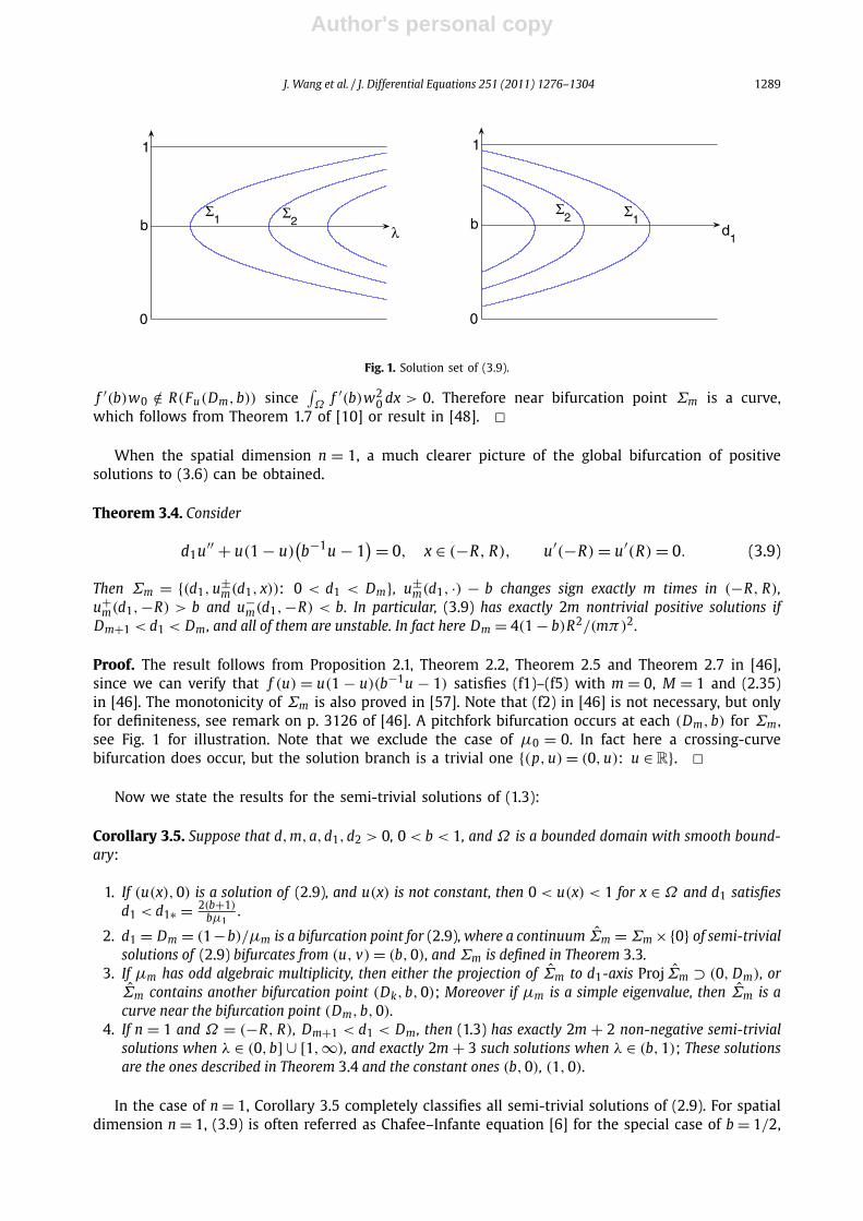
Fig. 1. Solution set of (3.9).
f ′(b)w0 /∈ R(Fu(Dm,b)) since∫Ω
f ′(b)w20 dx > 0. Therefore near bifurcation point Σm is a curve,
which follows from Theorem 1.7 of [10] or result in [48]. �When the spatial dimension n = 1, a much clearer picture of the global bifurcation of positive
solutions to (3.6) can be obtained.
Theorem 3.4. Consider
d1u′′ + u(1 − u)(b−1u − 1
) = 0, x ∈ (−R, R), u′(−R) = u′(R) = 0. (3.9)
Then Σm = {(d1, u±m(d1, x)): 0 < d1 < Dm}, u±
m(d1, ·) − b changes sign exactly m times in (−R, R),u+
m(d1,−R) > b and u−m(d1,−R) < b. In particular, (3.9) has exactly 2m nontrivial positive solutions if
Dm+1 < d1 < Dm, and all of them are unstable. In fact here Dm = 4(1 − b)R2/(mπ)2 .
Proof. The result follows from Proposition 2.1, Theorem 2.2, Theorem 2.5 and Theorem 2.7 in [46],since we can verify that f (u) = u(1 − u)(b−1u − 1) satisfies (f1)–(f5) with m = 0, M = 1 and (2.35)in [46]. The monotonicity of Σm is also proved in [57]. Note that (f2) in [46] is not necessary, but onlyfor definiteness, see remark on p. 3126 of [46]. A pitchfork bifurcation occurs at each (Dm,b) for Σm ,see Fig. 1 for illustration. Note that we exclude the case of μ0 = 0. In fact here a crossing-curvebifurcation does occur, but the solution branch is a trivial one {(p, u) = (0, u): u ∈ R}. �
Now we state the results for the semi-trivial solutions of (1.3):
Corollary 3.5. Suppose that d,m,a,d1,d2 > 0, 0 < b < 1, and Ω is a bounded domain with smooth bound-ary:
1. If (u(x),0) is a solution of (2.9), and u(x) is not constant, then 0 < u(x) < 1 for x ∈ Ω and d1 satisfiesd1 < d1∗ = 2(b+1)
bμ1.
2. d1 = Dm = (1−b)/μm is a bifurcation point for (2.9), where a continuum Σm = Σm ×{0} of semi-trivialsolutions of (2.9) bifurcates from (u, v) = (b,0), and Σm is defined in Theorem 3.3.
3. If μm has odd algebraic multiplicity, then either the projection of Σm to d1-axis Proj Σm ⊃ (0, Dm), orΣm contains another bifurcation point (Dk,b,0); Moreover if μm is a simple eigenvalue, then Σm is acurve near the bifurcation point (Dm,b,0).
4. If n = 1 and Ω = (−R, R), Dm+1 < d1 < Dm, then (1.3) has exactly 2m + 2 non-negative semi-trivialsolutions when λ ∈ (0,b] ∪ [1,∞), and exactly 2m + 3 such solutions when λ ∈ (b,1); These solutionsare the ones described in Theorem 3.4 and the constant ones (b,0), (1,0).
In the case of n = 1, Corollary 3.5 completely classifies all semi-trivial solutions of (2.9). For spatialdimension n = 1, (3.9) is often referred as Chafee–Infante equation [6] for the special case of b = 1/2,
Author's personal copy
1290 J. Wang et al. / J. Differential Equations 251 (2011) 1276–1304
which is the balanced case. Here all results for (3.6) are for higher-dimensional domains and b ∈ (0,1)
(balanced and unbalanced cases, see [46]).
4. A priori estimates and nonexistence of solutions
In this section we discuss the nonexistence of nonconstant positive solutions of (2.9) for certainparameter ranges. First we have the following a priori estimate for any non-negative solutions for (2.9),using similar argument as the proof of Theorem 2.1 part (c) with d1 = d2.
Lemma 4.1. Suppose that (u(x), v(x)) is a non-negative solution of (2.9). Then either (u, v) is a semi-trivialsolution in form of (u(x),0) where u satisfies (3.6), or for x ∈ Ω , (u(x), v(x)) satisfies
0 < u(x) < 1, and 0 < v(x) < C∗ = (1 − b)2
4bd+ d1
d2, (4.1)
where d,d1,d2,a,m > 0 and 0 < b < 1.
Proof. Let (u(x), v(x)) be a non-negative solution of (2.9). If there exists x0 ∈ Ω such that v(x0) = 0,then v(x) ≡ 0 from the strong maximum principle and u(x) satisfies (3.6). Similarly if u(x0) = 0 forsome x0 ∈ Ω , we also have u(x) ≡ 0 which also implies v ≡ 0. Otherwise u(x) > 0 and v(x) > 0 forx ∈ Ω .
From Lemma 3.2, u(x) � 1 and from the strong maximum principle, u(x) < 1 for all x ∈ Ω . Byadding the two equations in (2.9), we have
−(d1�u + d2�v) = u(1 − u)(b−1u − 1
) − dv
= u
((1 − u)
(b−1u − 1
) + dd1
d2
)− d
d2(d1u + d2 v)
�(
(1 − b)2
4b+ dd1
d2
)− d
d2(d1u + d2 v).
Then the maximum principle implies that
d1u + d2 v <1
d
((1 − b)2d2
4b+ dd1
),
which implies the desired estimate. �Now we can show the nonexistence of positive steady state solutions when the diffusion coeffi-
cients d1 and d2 are large.
Theorem 4.2. For any fixed m,a,d > 0 and 0 < b < 1, there exists d∗ = d∗(m,a,b,d,Ω) such that ifmin{d1,d2} > d∗ , then the only non-negative solutions to (2.9) are (0,0), (b,0), (1,0) and (λ, vλ).
Proof. Let (u, v) be a non-negative solution of (2.9), and denote u = |Ω|−1∫Ω
u dx, v = |Ω|−1∫Ω
v dx.Then ∫
Ω
(u − u)dx =∫Ω
(v − v)dx = 0. (4.2)
Author's personal copy
J. Wang et al. / J. Differential Equations 251 (2011) 1276–1304 1291
Multiplying the first equation in (2.9) by u − u and applying Lemma 4.1, we get
d1
∫Ω
∣∣∇(u − u)∣∣2
dx
=∫Ω
(u − u)u(1 − u)(b−1u − 1
)dx −
∫Ω
muv(u − u)
a + udx
=∫Ω
(u − u)u(1 − u)(b−1u − 1
)dx −
∫Ω
mv(u − u)2
a + udx −
∫Ω
mvu(u − u)
a + udx
� 2(b + 1)
b
∫Ω
(u − u)2 dx +∫Ω
−mvu(u − u)
a + udx. (4.3)
In a similar manner, we multiply the second equation in (2.9) by v − v to have
d2
∫Ω
∣∣∇(v − v)∣∣2
dx =∫Ω
(−d + mu
a + u
)(v − v)2 dx +
∫Ω
(−d + mu
a + u
)v(v − v)dx
=∫Ω
(−d + mu
a + u
)(v − v)2 dx +
∫Ω
muv
a + u(v − v)dx
�∫Ω
(−d + m
a + 1
)(v − v)2 dx +
∫Ω
muv
a + u(v − v)dx. (4.4)
Furthermore, adding the two equations in (2.9) and integrating over Ω , we get∫Ω
(−d1�u − d2�v)dx =∫Ω
[u(1 − u)
(b−1u − 1
) − dv]
dx, (4.5)
then the Neumann boundary conditions lead to
d
∫Ω
v dx =∫Ω
u(1 − u)(b−1u − 1
)dx � |Ω|
4b. (4.6)
Here we use the fact that |u(1 − u)| � 1/4 and |b−1u − 1| � b−1 for 0 � u � 1 (we know that0 � u(x) � 1 from Theorem 2.1). Thus
v = 1
|Ω|∫Ω
v dx � 1
4bd. (4.7)
From (4.7) and (4.2), we have∫Ω
muv
a + u(v − v)dx =
∫Ω
muv
a + u(v − v)dx −
∫Ω
muv
a + u(v − v)dx
=∫Ω
amv(v − v)
(a + u)(a + u)(u − u)dx
Author's personal copy
1292 J. Wang et al. / J. Differential Equations 251 (2011) 1276–1304
� m
4abd
∫Ω
|u − u||v − v|dx
� m
8abd
∫Ω
(u − u)2 dx + m
8abd
∫Ω
(v − v)2 dx, (4.8)
and similarly
∫Ω
−mvu
a + u(u − u)dx =
∫Ω
mu
(v
a + u− v
a + u
)(u − u)dx
=∫Ω
mu(u − u)
(a + u)(a + u)
[v(u − u) + (a + u)(v − v)
]dx
� m
4abd
∫Ω
(u − u)2 dx + m
a
∫Ω
|u − u||v − v|dx
� m
4abd
∫Ω
(u − u)2 dx + m
2a
∫Ω
(u − u)2 dx + m
2a
∫Ω
(v − v)2 dx. (4.9)
From (4.3), (4.4), (4.8) and (4.9) and the Poincaré inequality, we obtain that
d2
∫Ω
∣∣∇(v − v)2∣∣dx + d1
∫Ω
∣∣∇(u − u)2∣∣dx
� 1
μ1
(A
∫Ω
∣∣∇(v − v)2∣∣dx + B
∫Ω
∣∣∇(u − u)2∣∣dx
),
where
A = −d + m
a + 1+ m
2a
(1 + 1
4bd
), B = 2(b + 1)
b+ m
2a
(1 + 3
4bd
).
This shows that if
min{d1,d2} >1
μ1max{A, B},
then
∇(u − u) = ∇(v − v) = 0,
and (u, v) must be a constant solution. �
Author's personal copy
J. Wang et al. / J. Differential Equations 251 (2011) 1276–1304 1293
Remark 4.3.
1. One can make an apparent comparison of the results of Theorem 4.2 and Theorem 3.3(b) (orCorollary 3.5(a)) to see that
d∗ = 1
μ1max{A, B} � B
μ1>
2(b + 1)
bμ1= d1∗.
Note that Theorem 4.2 holds for any fixed a,b,m,d or equivalently any λ > 0.2. An earlier result in [8] implies the nonexistence of spatial nonhomogeneous patterns for general
reaction–diffusion systems when the diffusion coefficients are large. Our results here are morespecific to the model (1.3).
5. Bifurcation analysis and existence of steady states
5.1. Determination of bifurcation points
To prove the existence of nonconstant steady state solutions and periodic solutions of (1.3), wefurther analyze the stability/instability of the constant coexistence steady state (λ, vλ). Recall fromSection 3.1, the precise stability information of (λ, vλ) is determined by the trace and determinantof J i (i � 0), which are defined in (3.5) with A(λ), B(λ) and C(λ) defined in (3.4).
For that purpose, we define
T (λ, p) = −p(d1 + d2) + A(λ),
D(λ, p) = d1d2 p2 − d2 A(λ)p − B(λ)C(λ). (5.1)
We call the set {(λ, p) ∈ R2+: T (λ, p) = 0} to be the Hopf bifurcation curve, and the set{(λ, p) ∈ R2+: D(λ, p) = 0} to be the steady state bifurcation curve. The studies in [23,60] showthat the geometric properties of the Hopf and steady state bifurcation curves play important role inthe bifurcation analysis of (1.3).
First for the Hopf bifurcation curve, we notice that T (λ, p) = 0 is equivalent to p = A(λ)/(d1 +d2).Recall from Section 3.1,
A(λ) = λ
b(a + λ)
(−3λ2 + 2(b + 1 − a)λ + a(1 + b) − b).
The following lemma characterizes the profile of the function A(λ), and its proof is straightforwardcalculation thus omitted:
Lemma 5.1. Suppose that a > 0, 0 < b < 1, then there exist 0 < λ∗ < λ < 1 such that:
(a) If a(1 + b) − b � 0, then A(λ) > 0 in (0, λ) and A(0) = A(λ) = 0;(b) If a(1 + b) − b < 0, then there exists λc ∈ (0, λ∗) such that A(λ) < 0 in (0, λc); A(λ) > 0 in (λc, λ) and
A(0) = A(λc) = A(λ) = 0;(c) For either case, A′(λ) > 0 in (max{0, λc}, λ∗); A′(λ) < 0 in (λ∗, λ); A′(λ∗) = 0 and A(λ) attains its
maximum M∗ at λ∗ for λ ∈ [0,1]. Moreover M∗ satisfies
1 − b = A(b) � M∗ � (b2 + 1 − b + a(1 + b) + a2)
3b(a + 1).
Author's personal copy
1294 J. Wang et al. / J. Differential Equations 251 (2011) 1276–1304
Secondly for the steady state bifurcation curve D(λ, p) = 0, we notice that it is equivalent toD(λ, p) ≡ (a + λ)D(λ, p) = 0 for λ � 0. For fixed p, D is a degree 3 polynomial of λ, and for fixed λ,it is quadratic in p. Indeed we can solve p from D(p, λ) = 0,
p = p±(λ) :=d2 A(λ) ±
√d2
2 A2(λ) + 4d1d2 B(λ)C(λ)
2d1d2. (5.2)
One can also see that the function D(p, λ) has no critical points in the first quadrant, hence the set{(λ, p) ∈ R2+: D(λ, p) = 0} must be a bounded connected smooth curve.
Let S(λ) = d22 A2(λ) + 4d1d2 B(λ)C(λ). There exists a unique root of S(λ) = 0 denoted by λs , and
p±(λ) exists only for λ � λs . It is easy to verify that
S(b) = d22 A2(b) > 0 and S(λ) = 4d1d2 B(λ)C(λ) < 0,
so λs ∈ (b, λ). We can summarize the properties of p±(λ) as follows:
Lemma 5.2. Let p±(λ) be the functions defined in (5.2). Then there exists a λs ∈ (b, λ) such that p+(λ) existsfor λ ∈ [0, λs], and p−(λ) exists for λ ∈ [b, λs]. Moreover
limλ→λs
p+(λ) = limλ→λs
p−(λ) = A(λs)
2d1,
and
p+(0) =√
d
d1d2, p−(b) = 0.
Hence the steady state bifurcation curve {D(λ, p) = 0: p � 0, λ � 0} is a smooth curve connecting (λ, p) =(0,
√d
d1d2), (λ, p) = (λs,
A(λs)2d1
) and (λ, p) = (b,0). Moreover, p+(λ) attains its maximum value M∗∗ at
λ∗∗ ∈ [b, λs] thus the steady state bifurcation curve exists only for p ∈ [0, M∗∗], and M∗∗ can be estimated as
1 − b
d1= p+(b) � M∗∗ � M∗
d1� b2 + 1 − b + a(1 + b) + a2
3d1b(a + 1).
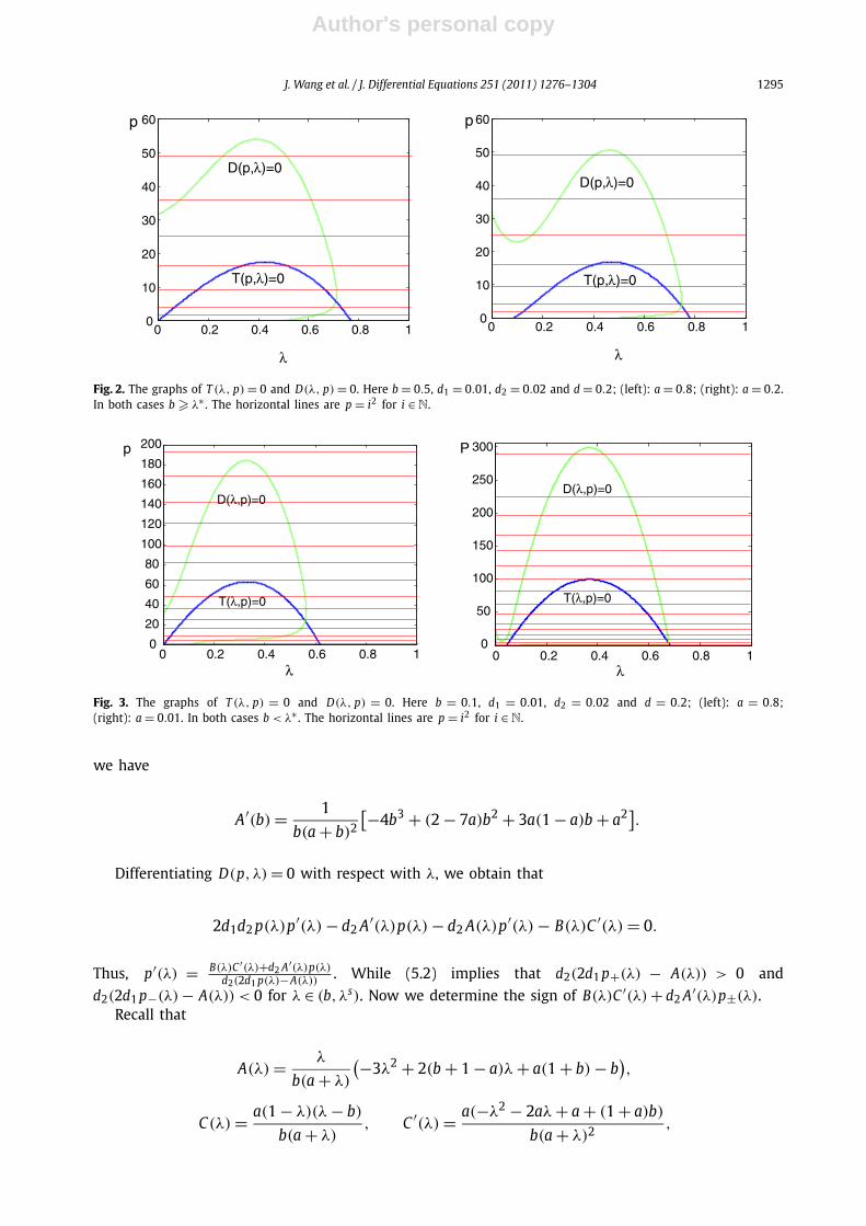
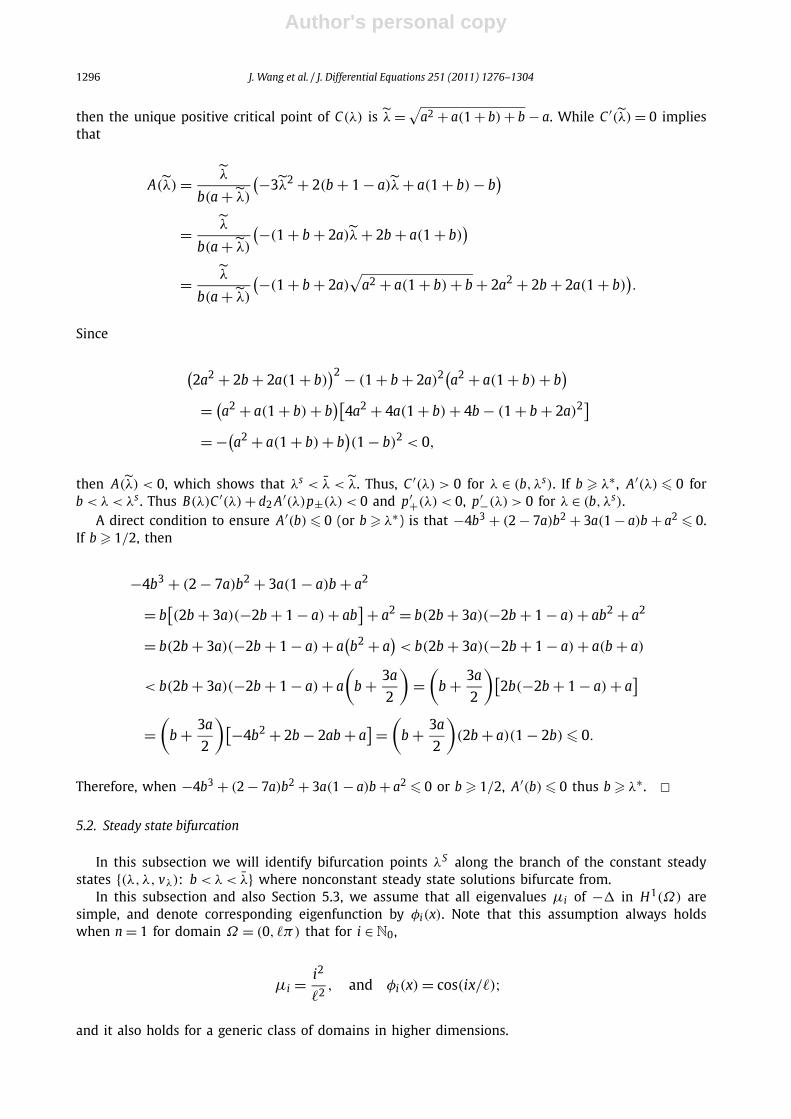
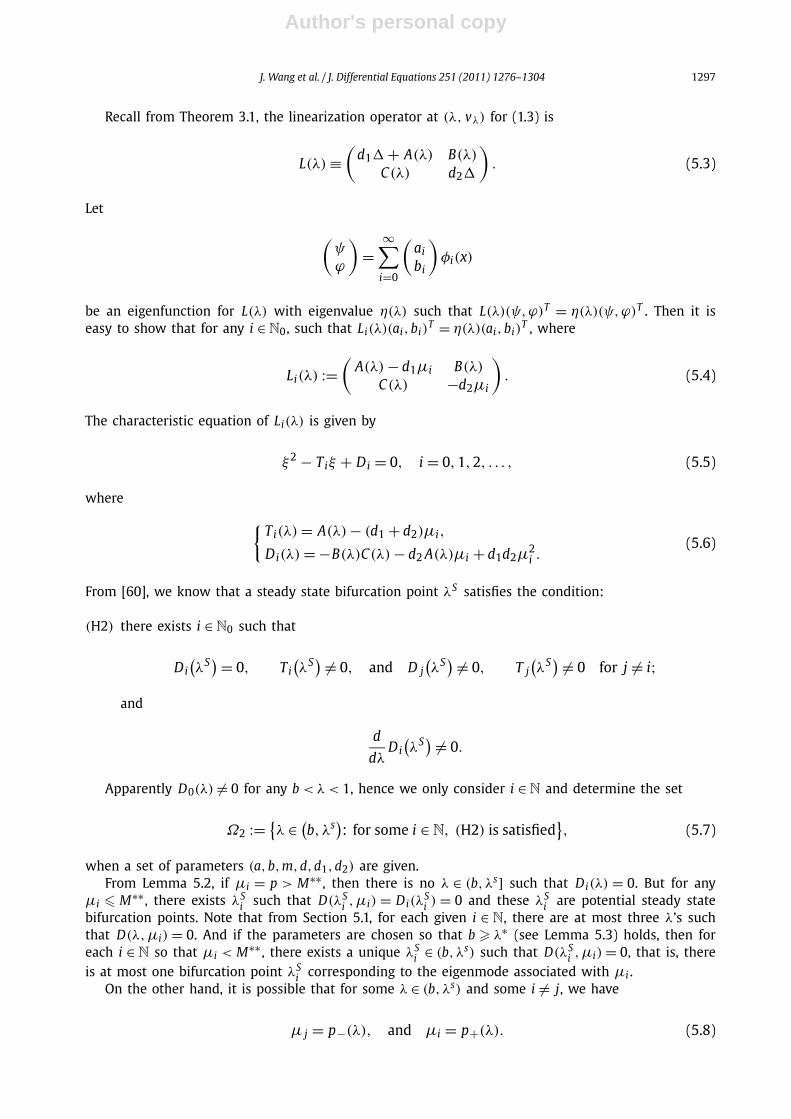
Figs. 2 and 3 show several possible graphs of the Hopf and steady state bifurcation curves. FromTheorem 3.1, the constant coexistence equilibrium (λ, vλ) is locally stable for λ ∈ (λ,1). Hence pos-sible bifurcation from (λ, vλ) can only occur for λ ∈ (b, λ). We prove a monotonicity result of p±(λ)
for λ ∈ (b, λs).
Lemma 5.3. Let λ∗ be the maximum point of A(λ) as defined in Lemma 5.1. If b � λ∗ , then p+(λ) is decreasingand p−(λ) is increasing for b < λ < λs . Moreover, if −4b3 + (2 − 7a)b2 + 3a(1 − a)b + a2 � 0 or b � 1/2,then b � λ∗ holds.
Proof. Since
A(λ) = λ
b(a + λ)
(−3λ2 + 2(b + 1 − a)λ + a(1 + b) − b),
A′(λ) = 1
b(a + λ)2
[−6λ3 + (2(1 + b) − 11a
)λ2 + 4a(1 + b − a)λ + a2(1 + b) − ab
],
Author's personal copy
J. Wang et al. / J. Differential Equations 251 (2011) 1276–1304 1295
Fig. 2. The graphs of T (λ, p) = 0 and D(λ, p) = 0. Here b = 0.5, d1 = 0.01, d2 = 0.02 and d = 0.2; (left): a = 0.8; (right): a = 0.2.In both cases b � λ∗ . The horizontal lines are p = i2 for i ∈ N.
Fig. 3. The graphs of T (λ, p) = 0 and D(λ, p) = 0. Here b = 0.1, d1 = 0.01, d2 = 0.02 and d = 0.2; (left): a = 0.8;(right): a = 0.01. In both cases b < λ∗ . The horizontal lines are p = i2 for i ∈ N.
we have
A′(b) = 1
b(a + b)2
[−4b3 + (2 − 7a)b2 + 3a(1 − a)b + a2].Differentiating D(p, λ) = 0 with respect with λ, we obtain that
2d1d2 p(λ)p′(λ) − d2 A′(λ)p(λ) − d2 A(λ)p′(λ) − B(λ)C ′(λ) = 0.
Thus, p′(λ) = B(λ)C ′(λ)+d2 A′(λ)p(λ)d2(2d1 p(λ)−A(λ))
. While (5.2) implies that d2(2d1 p+(λ) − A(λ)) > 0 andd2(2d1 p−(λ) − A(λ)) < 0 for λ ∈ (b, λs). Now we determine the sign of B(λ)C ′(λ) + d2 A′(λ)p±(λ).
Recall that
A(λ) = λ
b(a + λ)
(−3λ2 + 2(b + 1 − a)λ + a(1 + b) − b),
C(λ) = a(1 − λ)(λ − b)
b(a + λ), C ′(λ) = a(−λ2 − 2aλ + a + (1 + a)b)
b(a + λ)2,
Author's personal copy
1296 J. Wang et al. / J. Differential Equations 251 (2011) 1276–1304
then the unique positive critical point of C(λ) is λ = √a2 + a(1 + b) + b − a. While C ′ (λ) = 0 implies
that
A(λ) = λ
b(a + λ)
(−3λ2 + 2(b + 1 − a)λ + a(1 + b) − b)
= λ
b(a + λ)
(−(1 + b + 2a)λ + 2b + a(1 + b))
= λ
b(a + λ)
(−(1 + b + 2a)√
a2 + a(1 + b) + b + 2a2 + 2b + 2a(1 + b)).
Since
(2a2 + 2b + 2a(1 + b)
)2 − (1 + b + 2a)2(a2 + a(1 + b) + b)
= (a2 + a(1 + b) + b
)[4a2 + 4a(1 + b) + 4b − (1 + b + 2a)2]
= −(a2 + a(1 + b) + b
)(1 − b)2 < 0,
then A(λ) < 0, which shows that λs < λ < λ. Thus, C ′(λ) > 0 for λ ∈ (b, λs). If b � λ∗ , A′(λ) � 0 forb < λ < λs . Thus B(λ)C ′(λ) + d2 A′(λ)p±(λ) < 0 and p′+(λ) < 0, p′−(λ) > 0 for λ ∈ (b, λs).
A direct condition to ensure A′(b) � 0 (or b � λ∗) is that −4b3 + (2 − 7a)b2 + 3a(1 − a)b + a2 � 0.If b � 1/2, then
−4b3 + (2 − 7a)b2 + 3a(1 − a)b + a2
= b[(2b + 3a)(−2b + 1 − a) + ab
] + a2 = b(2b + 3a)(−2b + 1 − a) + ab2 + a2
= b(2b + 3a)(−2b + 1 − a) + a(b2 + a
)< b(2b + 3a)(−2b + 1 − a) + a(b + a)
< b(2b + 3a)(−2b + 1 − a) + a
(b + 3a
2
)=
(b + 3a
2
)[2b(−2b + 1 − a) + a
]=
(b + 3a
2
)[−4b2 + 2b − 2ab + a] =
(b + 3a
2
)(2b + a)(1 − 2b) � 0.
Therefore, when −4b3 + (2 − 7a)b2 + 3a(1 − a)b + a2 � 0 or b � 1/2, A′(b) � 0 thus b � λ∗ . �5.2. Steady state bifurcation
In this subsection we will identify bifurcation points λS along the branch of the constant steadystates {(λ,λ, vλ): b < λ < λ} where nonconstant steady state solutions bifurcate from.
In this subsection and also Section 5.3, we assume that all eigenvalues μi of −� in H1(Ω) aresimple, and denote corresponding eigenfunction by φi(x). Note that this assumption always holdswhen n = 1 for domain Ω = (0, �π) that for i ∈ N0,
μi = i2
�2, and φi(x) = cos(ix/�);
and it also holds for a generic class of domains in higher dimensions.
Author's personal copy
J. Wang et al. / J. Differential Equations 251 (2011) 1276–1304 1297
Recall from Theorem 3.1, the linearization operator at (λ, vλ) for (1.3) is
L(λ) ≡(
d1� + A(λ) B(λ)
C(λ) d2�
). (5.3)
Let (ψ
ϕ
)=
∞∑i=0
(aibi
)φi(x)
be an eigenfunction for L(λ) with eigenvalue η(λ) such that L(λ)(ψ,ϕ)T = η(λ)(ψ,ϕ)T . Then it iseasy to show that for any i ∈ N0, such that Li(λ)(ai,bi)
T = η(λ)(ai,bi)T , where
Li(λ) :=(
A(λ) − d1μi B(λ)
C(λ) −d2μi
). (5.4)
The characteristic equation of Li(λ) is given by
ξ2 − Tiξ + Di = 0, i = 0,1,2, . . . , (5.5)
where {Ti(λ) = A(λ) − (d1 + d2)μi,
Di(λ) = −B(λ)C(λ) − d2 A(λ)μi + d1d2μ2i .
(5.6)
From [60], we know that a steady state bifurcation point λS satisfies the condition:
(H2) there exists i ∈ N0 such that
Di(λS) = 0, Ti
(λS) = 0, and D j
(λS) = 0, T j
(λS) = 0 for j = i;
and
d
dλDi
(λS) = 0.
Apparently D0(λ) = 0 for any b < λ < 1, hence we only consider i ∈ N and determine the set
Ω2 := {λ ∈ (
b, λs): for some i ∈ N, (H2) is satisfied}, (5.7)
when a set of parameters (a,b,m,d,d1,d2) are given.From Lemma 5.2, if μi = p > M∗∗ , then there is no λ ∈ (b, λs] such that Di(λ) = 0. But for any
μi � M∗∗ , there exists λSi such that D(λS
i ,μi) = Di(λSi ) = 0 and these λS
i are potential steady statebifurcation points. Note that from Section 5.1, for each given i ∈ N, there are at most three λ’s suchthat D(λ,μi) = 0. And if the parameters are chosen so that b � λ∗ (see Lemma 5.3) holds, then foreach i ∈ N so that μi < M∗∗ , there exists a unique λS
i ∈ (b, λs) such that D(λSi ,μi) = 0, that is, there
is at most one bifurcation point λSi corresponding to the eigenmode associated with μi .
On the other hand, it is possible that for some λ ∈ (b, λs) and some i = j, we have
μ j = p−(λ), and μi = p+(λ). (5.8)
Author's personal copy
1298 J. Wang et al. / J. Differential Equations 251 (2011) 1276–1304
Then for this λ, 0 is not a simple eigenvalue of L(λ) and we shall not consider bifurcations at suchpoints. However from an argument in [60], for n = 1 and Ω = (0, �π), there are only countablymany �, such that (5.8) occurs for some i = j. For general bounded domains in Rn , one can also showthat (5.8) does not occur for generic domains.
Next we verify dDidλ
(λSi ) = 0 if b � λ∗ and λS
i = λs . Indeed one has D ′i(λ) = −B(λ)C(λ)− d2μi A′(λ),
and from the proof of Lemma 5.3,
p′±(λ) = B(λ)C ′(λ) + d2 A′(λ)p±(λ)
d2(2d1 p±(λ) − A(λ)).
Therefore from Lemma 5.3, dDidλ
(λSi ) = 0 if b � λ∗ and λS
i = λs .Summarizing the above discussion and using a general bifurcation theorem [57], we obtain the
main result of this section on the global bifurcation of steady state solutions:
Theorem 5.4. Suppose that a,d,d1,d2 > 0 and 0 < b < 1 are fixed. Let Ω be a bounded smooth domain sothat its spectral set S = {μi} satisfy that:
[S1] All eigenvalues μi are simple for i � 0;[S2] There exists k ∈ N such that 0 = μ0 < μ1 < · · · < μk < M∗∗ < μk+1 , where M∗∗ is a constant depend-
ing on a,b,d,d1,d2 which is defined in Lemma 5.3,
and we also assume that b � λ∗ , then for each 1 � i � k, there exists a unique λSi ∈ (b, λ) such that
D(λSi ,μi) = 0. If in addition, we assume
λSi = λS
j , for any 1 � i = j � k, and λSi = λs, for any 1 � i � k, (5.9)
then:
1. There is a smooth curve Γi of positive solutions of (2.9) bifurcating from (λ, u, v) = (λSi , λS
i , vλSi), with
Γi contained in a global branch Ci of positive nontrivial solutions of (2.9);2. Near (λ, u, v) = (λS
i , λSi , vλS
i), Γi = {(λi(s), ui(s), vi(s)): s ∈ (−ε, ε)}, where ui(s) = λS
i +saiφi(x) + sψ1,i(s), vi(s) = λS
i + sbiφi(x) + sψ2,i(s) for some C∞ smooth functions λi,ψ1,i,ψ2,i suchthat λi(0) = λS
i and ψ1,i(0) = ψ2,i(0) = 0; Here (ai,bi) satisfies
L(λS
i
)[(ai,bi)
�φi(x)] = (0,0)�.
3. Either Ci contains another (λSj , λ
Sj , vλS
j) for j = i and 1 � j � k, or the projection of Ci onto λ-axis
contains the interval (0, λSi ), or Ci contains a solution in form (λ, uS ,0) for 0 < λ � 1 and uS > 0.
Proof. The existence and uniqueness of λSi follows from discussions above. Then the local bifurcation
result follows from Theorem 3.2 in [60], and it is an application of a more general result Theorem 4.3in [48].
For the global bifurcation, we apply Theorem 4.3 in [48]. After the change of variables:
w1 = u − λ, w2 = v − vλ, m = d(a + λ)
λ, vλ = λ(1 − λ)(b−1λ − 1)
d,
we define a nonlinear equation:
Author's personal copy
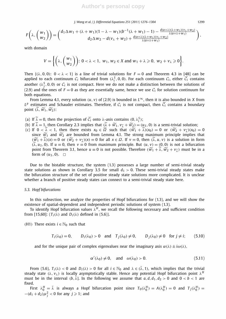
J. Wang et al. / J. Differential Equations 251 (2011) 1276–1304 1299
F
(λ,
(w1w2
))=
(d1�w1 + (λ + w1)(1 − λ − w1)(b−1(λ + w1) − 1) − d(a+λ)(λ+w1)(vλ+w2)
λ(a+λ+w1)
d2�w2 − d(vλ + w2) + d(a+λ)(λ+w1)(vλ+w2)λ(a+λ+w1)
),
with domain
V ={(
λ,
(w1w2
)): 0 < λ < 1, w1, w2 ∈ X and w1 + λ � 0, w2 + vλ � 0
}.
Then {(λ,0,0): 0 < λ < 1} is a line of trivial solutions for F = 0 and Theorem 4.3 in [48] can beapplied to each continuum Ci bifurcated from (λS
i ,0,0). For each continuum Ci , either Ci containsanother (λS
j ,0,0) or Ci is not compact. Here we do not make a distinction between the solutions of(2.9) and the ones of F = 0 as they are essentially same, hence we use Ci for solution continuum forboth equations.
From Lemma 4.1, every solution (u, v) of (2.9) is bounded in L∞ , then it is also bounded in X fromL p estimates and Schauder estimates. Therefore, if Ci is not compact, then Ci contains a boundarypoint (λ, w1, w2):
(a) If λ = 0, then the projection of Ci onto λ-axis contains (0, λSi );
(b) If λ = 1, then Corollary 2.3 implies that (λ + w1, v λ + w2) = (uS ,0) is a semi-trivial solution;(c) If 0 < λ < 1, then there exists x0 ∈ Ω such that (w1 + λ)(x0) = 0 or (w2 + v λ)(x0) = 0
since w1 and w2 are bounded from Lemma 4.1. The strong maximum principle implies that(w1 + λ)(x) ≡ 0 or (w2 + v λ)(x) ≡ 0 for all x ∈ Ω . If v ≡ 0, then (λ, u, v) is a solution in form(λ, uS ,0). If u ≡ 0, then v ≡ 0 from maximum principle. But (u, v) = (0,0) is not a bifurcationpoint from Theorem 3.1, hence u ≡ 0 is not possible. Therefore (w1 + λ, w2 + v λ) must be in aform of (uS ,0). �
Due to the bistable structure, the system (1.3) possesses a large number of semi-trivial steadystate solutions as shown in Corollary 3.5 for small d1 > 0. These semi-trivial steady states makethe bifurcation structure of the set of positive steady state solutions more complicated. It is unclearwhether a branch of positive steady states can connect to a semi-trivial steady state here.
5.3. Hopf bifurcations
In this subsection, we analyze the properties of Hopf bifurcations for (1.3), and we will show theexistence of spatial-dependent and independent periodic solutions of system (1.3).
To identify Hopf bifurcation values λH , we recall the following necessary and sufficient conditionfrom [15,60]: (Ti(λ) and Di(λ) defined in (5.6)).
(H1) There exists i ∈ N0 such that
Ti(λ0) = 0, Di(λ0) > 0 and T j(λ0) = 0, D j(λ0) = 0 for j = i; (5.10)
and for the unique pair of complex eigenvalues near the imaginary axis α(λ) ± iω(λ),
α′(λ0) = 0, and ω(λ0) > 0. (5.11)
From (5.6), Ti(λ) < 0 and Di(λ) > 0 for all i ∈ N0 and λ ∈ (λ,1), which implies that the trivialsteady state (λ, vλ) is locally asymptotically stable. Hence any potential Hopf bifurcation point λH
must be in the interval (b, λ]. In the following we assume that a,d,d1,d2 > 0 and 0 < b < 1 arefixed.
First λH0 = λ is always a Hopf bifurcation point since T0(λ
H0 ) = A(λH
0 ) = 0 and T j(λH0 ) =
−(d1 + d2)μ2j < 0 for any j � 1; and
Author's personal copy
1300 J. Wang et al. / J. Differential Equations 251 (2011) 1276–1304
Di(λH
0
) = −B(λH
0
)C(λH
0
) + d1d2μ2j > 0
for any j ∈ N0. This corresponds to the Hopf bifurcation of spatially homogeneous periodic orbitswhich have been known from the studies of Section 3 in [53]. Apparently λH
0 is also the unique valueλ for the Hopf bifurcation of spatially homogeneous periodic orbits from the uniqueness result oflimit cycle in [53].
Hence in the following we search for spatially nonhomogeneous Hopf bifurcation for i � 1 in (H1).Notice that A(b) > 0, A(λH
0 ) = 0 and A(λ) > 0 in (b, λH0 ). Similar to Theorem 5.4, we assume that
b � λ∗ , but we will comment on the case of b < λ∗ at the end of this section. Again we assume that[S1] holds, i.e. all eigenvalues μi are simple.
If b � λ∗ , then clearly A(λ) is strictly decreasing for λ ∈ (b, λ) from Lemma 5.1. We define λHi to
be the unique solution of A(λ) = (d1 + d2)μi satisfying b < λ < λ. These points satisfy
b < λHm < λH
m−1 < · · · < λH1 < λH
0 ,
where m is the largest integer so that μm < M∗/(d1 + d2), and M∗ is defined in Lemma 5.1. ClearlyTi(λ
Hi ) = 0 and T j(λ
Hi ) = 0 for any j = i. The condition Di(λ
Hi ) > 0 does not hold for all i satisfying
1 � i � m. Geometrically Di(λHi ) = D(λH
i ,μi) > 0 is equivalent to that the point (λHi ,μi) is in the
exterior of the curve D(λ, p) = 0 (see Figs. 2 and 3). From the monotonicity properties proved inLemma 5.3, the curves D(λ, p) = 0 and T (λ, p) have a unique intersection point (λ�, p�) for λ ∈ (b, λ)
and p > 0. Hence Di(λHi ) > 0 if λH
i > λ� while Di(λHi ) < 0 if λH
i < λ� . Finally D j(λHi ) = 0 if λH
i = λSj
for 1 � j � k, that is, a Hopf bifurcation point and a steady state bifurcation point do not overlap.Summarizing our analysis above and applying Theorem 2.1 in [60], we obtain the following results
on the Hopf bifurcations:
Theorem 5.5. Suppose that a,d,d1,d2 > 0 and 0 < b < 1 are fixed. Let Ω be a bounded smooth domain sothat its spectral set S = {μi} satisfies that [S1], and
[S3] There exists m ∈ N such that 0 = μ0 < μ1 < · · · < μm < M∗d1+d2
< μm+1 , where M∗ is a constant de-pending on a,b which is defined in Lemma 5.1,
and we also assume that b � λ∗ , then for each 1 � i � m, there exists a unique λHi ∈ (b, λ) such that
T (λHi ,μi) = 0, and there exist h ∈ N and h � m such that for 1 � i � h, D(λH
i ,μi) > 0. If in addition, weassume for 1 � i � h,
λHi = λS
j , for any 1 � j � k, (5.12)
where λSj (1 � j � k) are defined in Theorem 5.4, then for each 0 � i � h,
1. (1.3) undergoes a Hopf bifurcation at λ = λHj ; there is a smooth curve Λi of positive periodic orbits of (1.3)
bifurcating from (λ, u, v) = (λHi , λH
i , vλHi), with Λi contained in a global branch Pi of positive nontrivial
periodic orbits of (1.3).2. The bifurcating periodic orbits from λ = λH
0 are spatially homogeneous, which coincide with the periodicorbits of the corresponding ODE system (see [53]); the Hopf bifurcation at λ = λH
0 is supercritical andbackward; the bifurcating spatially homogeneous periodic orbits are locally asymptotically stable nearλ = λH
0 .3. The bifurcating periodic orbits from λ = λH
i with 1 � i � h are spatially nonhomogeneous; near bifurca-tion point, they are in a form of
(λ, u, v) = (λH
i + o(s), λHi + sei cos
(ω
(λH
i
)t)φi(x) + o(s), vλH
i+ sfi cos
(ω
(λH
i
)t)φi(x) + o(s)
),
Author's personal copy
J. Wang et al. / J. Differential Equations 251 (2011) 1276–1304 1301
for s ∈ (0, δ), where ω(λHi ) =
√Di(λ
Hi ) is the corresponding time frequency, φi(x) is the corresponding
spatial eigenfunction, and (ei, f i) is a corresponding eigenvector.4. The global branch of spatially homogenous periodic orbits P0 is a curve parameterized by λ ∈ (λ�, λ) from
results in [53]; the spatially homogeneous periodic orbit is unique for each λ ∈ (λ�, λ), and the period ofthe closed orbits approaches to ∞ as λ → (λ�)− , that is, the cycle converges to a loop of heteroclinic orbits,which exists only when λ = λ� .
5. For 1 � i � h, the global branch of spatially nonhomogeneous periodic orbits Pi satisfies: either Picontains another bifurcation point (λ, u, v) = (λH
j , λHj , vλH
j) for 1 � j � h and j = i, or Pi contains
a spatially homogenous periodic orbit on P0 , or the projection of Pi onto λ-axis contains the interval(0, λH
i ) or (λHi ,1), or there exists λ ∈ (0,1) such that there exists a sequence of spatially nonhomoge-
neous periodic orbits (λl, ul, vl) ∈ Pi such that λl → λ and the time period of (λl, ul, vl) tends to ∞ asl → ∞.
Proof. The local bifurcation results in parts 1 and 3 follow from discussions in this section and The-orem 2.1 in [60], and parts 2 and 4 follow from [53] as any solutions of the ODE model are spatiallyhomogenous solutions of (1.3). The stability assertion in part 2 can be obtained in a similar way as[60] and the calculation in [53]. For the global bifurcation results, we use the one in Section 6.5in [58] for the abstract setting. Indeed to obtain the four alternatives stated here, we have to usea more general version of global bifurcation theorem restricted to the positive cone in the functionspace, which is similar to the corresponding result in [48] for steady state solutions. Note that fromTheorem 2.1, we know that all periodic orbits are uniformly bounded for λ ∈ [0,1]. �Remark 5.6.
1. Notice that Theorem 5.5 does not exclude a secondary bifurcation of spatial nonhomogeneousperiodic orbits from the branch of spatially homogenous periodic orbits P0. It is known from [53]that all spatially homogenous periodic orbits on P0 are locally asymptotically stable with respectto the ODE dynamics (which also implies the stability for PDE dynamics when d1 = d2), but it isnot known that whether the stability still hold for PDE dynamics for general diffusion coefficientsd1 = d2.
2. The conditions [S2] in Theorem 5.4 and [S3] in Theorem 5.5 are compatible, as we have shown inLemma 5.1 and Lemma 5.2. Hence the steady state bifurcation points λS
i (1 � i � k) and the Hopfbifurcation points λH
i (0 � i � h) could appear in an intertwining order (see example below).However the number k of steady state bifurcation in Theorem 5.4 and the number m or h inTheorem 5.5 are in general different, as clearly shown in Figs. 2 and 3. In all cases of Figs. 2 and3, the relation k > m > h holds.
3. For a given eigen-mode φi(x), if λSi and λH
i both exist, and the simplicity conditions (5.9) and(5.12) are both satisfied, then a steady state bifurcation always occurs at λ = λS
i with eigen-mode φi , but a Hopf bifurcation with eigen-mode φi occurs only if λS
i < λHi .
4. In both Theorem 5.4 and Theorem 5.5, we assume that b � λ∗ . Note that from Lemma 5.3, b > λ∗holds if b � 1/2 or a and b satisfy a more complicated algebraic condition. Fig. 2 shows thebifurcation points in this case. However the condition b � λ∗ is not necessary for the occur-rence of steady state or Hopf bifurcations. If b < λ∗ (see Fig. 3), then the curves D(λ, p) = 0 andT (λ, p) = 0 are not monotone with respect to λ, which implies even more bifurcation points. SeeExample 5.8 below.
To visualize the cascade of steady state or Hopf bifurcations, we consider two numerical examples.In both examples, we assume the spatial dimension n = 1 and Ω = (0,π).
Example 5.7. We use the parameter values in Fig. 2 (left). Notice that the horizontal lines inFig. 2 (left) are p = μi = i2 (the eigenvalues of � for Ω = (0,π)). Then the largest number k in[S2] of Theorem 5.4 so that a steady state bifurcation can occur is k = 7. On the other hand, the
Author's personal copy
1302 J. Wang et al. / J. Differential Equations 251 (2011) 1276–1304
largest number m in [S3] of Theorem 5.5 so that a Hopf bifurcation can occur is m = 4. But for the 4intersection points of T (λ, p) = 0 and p = μi , only two of them are outside of the curve D(λ, p) = 0,so the number h in Theorem 5.5 is h = 2. Therefore there exist 3 Hopf bifurcation points and 7 steadystate bifurcation points. The occurrence of bifurcations is in the order of
λH0 ≈ 0.7698 > λH
1 ≈ 0.7601 > λH2 ≈ 0.7292 > λS
3 ≈ 0.7135 > λS2 ≈ 0.6985 > λS
4 ≈ 0.6983
> λS5 ≈ 0.6660 > λS
6 ≈ 0.6131 > λS1 ≈ 0.5847 > λS
7 ≈ 0.5126 > b = 0.5.
Here none of these bifurcation points overlap with each other, which assures the simplicity of eigen-value with zero real part. One can also find that the heteroclinic bifurcation point is λ� ≈ 0.7670,which is between the first two Hopf bifurcation points. Hence a spatially homogeneous periodic orbitonly exists for λ� ≈ 0.7670 < λ < 0.7698 ≈ λH
0 .
Example 5.8. We use the parameter values in Fig. 3 (left). Then similar to Example 5.8, we havek = 13, m = 7 and h = 4 respectively. There are 5 Hopf bifurcation points for the eigen-mode 0 � i � 4.For 1 � i � 9, there is a single steady state bifurcation point λS
i , but for 10 � i � 13, there are 2 steadystate bifurcation points (which we call λS
i,±) for each eigen-mode i. Hence totally there are 17 steadystate bifurcation points. The occurrence of bifurcations is in the order of
λH0 ≈ 0.6196 > λH
1 ≈ 0.6174 > λH2 ≈ 0.6106 > λH
3 ≈ 0.5990 > λH4 ≈ 0.5817 > λS
6 ≈ 0.5630
> λS5 ≈ 0.5595 > λS
7 ≈ 0.5589 > λS8 ≈ 0.5497 > λS
4 ≈ 0.5409 > λS9 ≈ 0.5362
> λS10,+ ≈ 0.5181 > λS
11,+ ≈ 0.4943 > λS3 ≈ 0.4724 > λS
12,+ ≈ 0.4621
> λS13,+ ≈ 0.4117 > λS
13,− ≈ 0.2415 > λS2 ≈ 0.1894 > λS
12,− ≈ 0.1847
> λS11,− ≈ 0.1455 > λS
10,− ≈ 0.1142 > λS1 ≈ 0.1127 > b = 0.1.
Note that here the heteroclinic bifurcation point λ� ≈ 0.6123, which is between λH1 and λH
2 .
Examples 5.7 and 5.8 demonstrate the richness of spatial and spatiotemporal patterns for λ be-tween λ = b (system threshold value) and λ = λ (primary Hopf bifurcation point).
6. Conclusions
Reaction–diffusion predator–prey models with strong Allee effect in prey such as (1.3) have beenproposed in [35,39,40], and numerical simulation have shown that the system (1.3) is capable to gen-erate complicated spatiotemporal dynamics. In this paper we rigorously prove some general behaviorof the dynamical equation (1.3): for λ > 1, the predator is destined to go extinct (Theorem 2.1(c));and for large predator initial values, both predator and prey go extinct (Theorem 2.4). The latter re-sult confirms the overexploitation phenomenon still exists with the addition of the diffusion. Withstrong Allee effect in prey, extinction for both species is always a locally stable equilibrium. But forλ over the threshold value b, there always exist some other spatiotemporal patterns (steady state oroscillatory ones) (Theorems 5.4 and 5.5). These patterns are usually unstable, and they may lie on athreshold manifold which separates the basin of attraction of the extinction equilibrium and all otherpersistent orbits. The threshold manifold may also contain a large number of semi-trivial prey-onlysteady state solutions (Corollary 3.5).
Compared with the ODE dynamics classified in [53], the PDE dynamics shown here is still coarse.It would be interesting to know whether a global separatrix for the bistable dynamics exists. In ODEdynamics, the separatrix is simply the stable manifold of the threshold equilibrium (b,0). Our analysisdoes show that for the parameter range that the ODE system possesses a limit cycle, the correspond-ing PDE could have more patterned solutions (Theorems 5.4, 5.5 and Examples 5.7, 5.8). Comparison
Author's personal copy
J. Wang et al. / J. Differential Equations 251 (2011) 1276–1304 1303
with the ODE dynamics also suggests a conjecture that when λ � b, the extinction equilibrium isglobally asymptotic stable. In general, it is useful to know conditions on initial conditions for thepopulations to persist, and the existence of large amplitude patterned steady state or oscillatory solu-tions far away from bifurcation points is also not known.
Our analysis here can also be generalized to diffusive predator–prey system with strong Allee effectlike (1.1) but with more general functional responses and growth rates (see [53] for such functions).Bifurcation structure in higher-dimensional domains can also be more complex than the ones shownin Examples 5.7 and 5.8.
Acknowledgments
The authors thank anonymous referee for helpful suggestions. Jinfeng Wang would like to thankChris Cosner and Steve Cantrell for helpful discussion about Theorem 2.1 during ECNU summer schoolin 2009.
References
[1] N.D. Alikakos, An application of the invariance principle to reaction–diffusion equations, J. Differential Equations 33 (1979)201–225.
[2] W.C. Allee, Animal Aggregations: A Study in General Sociology, University of Chicago Press, 1931.[3] S.D. Boukal, W.M. Sabelis, L. Berec, How predator functional responses and Allee effects in prey affect the paradox of
enrichment and population collapses, Theoret. Popul. Biol. 72 (2007) 136–147.[4] R.S. Cantrell, C. Cosner, V. Hutson, Permanence in ecological systems with spatial heterogeneity, Proc. Roy. Soc. Edinburgh
Sect. A 123 (1993) 533–559.[5] R.S. Cantrell, C. Cosner, Spatial Ecology via Reaction–Diffusion Equations, Wiley Ser. Math. Comput. Biol., John Wiley &
Sons, Ltd., 2003.[6] N. Chafee, E.F. Infante, A bifurcation problem for a nonlinear partial differential equation of parabolic type, Appl. Anal. 4
(1974/1975) 17–37.[7] X.-Y. Chen, P. Polácik, Gradient-like structure and Morse decompositions for time-periodic one-dimensional parabolic equa-
tions, J. Dynam. Differential Equations 7 (1) (1995) 73–107.[8] E. Conway, D. Hoff, J. Smoller, Large time behavior of solutions of systems of nonlinear reaction–diffusion equations, SIAM
J. Appl. Math. 35 (1) (1978) 1–16.[9] F. Courchamp, L. Berec, J. Gascoigne, Allee Effects in Ecology and Conservation, Oxford University Press, 2008.
[10] M.G. Crandall, P.H. Rabinowitz, Bifurcation from simple eigenvalues, J. Funct. Anal. 8 (1971) 321–340.[11] Y.-H. Du, J.-P. Shi, Some recent results on diffusive predator–prey models in spatially heterogeneous environment, in:
Nonlinear Dynamics and Evolution Equations, in: Fields Inst. Commun., vol. 48, Amer. Math. Soc., Providence, RI, 2006,pp. 95–135.
[12] Y.-H. Du, J.-P. Shi, A diffusive predator–prey model with a protection zone, J. Differential Equations 229 (1) (2006) 63–91.[13] Y.-H. Du, J.-P. Shi, Allee effect and bistability in a spatially heterogeneous predator–prey model, Trans. Amer. Math.
Soc. 359 (9) (2007) 4557–4593.[14] J.K. Hale, Asymptotic Behavior of Dissipative Systems, Math. Surveys Monogr., vol. 25, Amer. Math. Soc., Providence, RI,
1988.[15] B.D. Hassard, N.D. Kazarinoff, Y.-H. Wan, Theory and Applications of Hopf Bifurcation, Cambridge University Press, Cam-
bridge, 1981.[16] D. Henry, Geometric Theory of Semilinear Parabolic Equations, Lecture Notes in Math., vol. 840, Springer-Verlag, Berlin/New
York, 1981.[17] C.S. Holling, The components of predation as revealed by a study of small mammal predation of the European Pine Sawfly,
Canad. Entomol. 91 (1959) 293–320.[18] S.L. Hollis, R.H. Martin, M. Pierre, Global existence and boundedness in reaction–diffusion systems, SIAM J. Math.
Anal. 18 (3) (1987) 744–761.[19] J.-H. Huang, G. Lu, S.-G. Ruan, Existence of traveling wave solutions in a diffusive predator–prey model, J. Math. Biol. 46 (2)
(2003) 132–152.[20] J.-F. Jiang, X. Liang, X.-Q. Zhao, Saddle-point behavior for monotone semiflows and reaction–diffusion models, J. Differential
Equations 203 (2) (2004) 313–330.[21] J.-F. Jiang, J.-P. Shi, Dynamics of a reaction–diffusion system of autocatalytic chemical reaction, Discrete Contin. Dyn.
Syst. 21 (1) (2008) 245–258.[22] J.-F. Jiang, J.-P. Shi, Bistability dynamics in some structured ecological models, in: R.S. Cantrell, C. Cosner, S.-G. Ruan (Eds.),
Spatial Ecology, Chapman & Hall/CRC, 2009.[23] J.-Y. Jin, J.-P. Shi, J.-J. Wei, F.-Q. Yi, Bifurcations of patterned solutions in diffusive Lengyel–Epstein system of CIMA chemical
reaction, Rocky Mountain J. Math. (2011), in press.[24] N. Kazarinov, P. van den Driessche, A model predator–prey systems with functional response, Math. Biosci. 39 (1978) 125–
134.
Author's personal copy
1304 J. Wang et al. / J. Differential Equations 251 (2011) 1276–1304
[25] W. Ko, K. Ryu, Qualitative analysis of a predator–prey model with Holling type II functional response incorporating a preyrefuge, J. Differential Equations 231 (2006) 534–550.
[26] M.A. Lewis, P. Karevia, Allee dynamics and the spread of invading organisms, Theoret. Popul. Biol. 43 (1993) 141–158.[27] A.J. Lotka, Elements of Physical Biology, Williams and Wilkins, Baltimore, 1925.[28] Y. Lou, W.-M. Ni, Diffusion, self-diffusion and cross-diffusion, J. Differential Equations 131 (1996) 79–131.[29] Y. Lou, W.-M. Ni, Diffusion vs cross-diffusion: an elliptic approach, J. Differential Equations 154 (1999) 157–190.[30] A.B. Medvinsky, S.V. Petrovskii, I.A. Tikhonova, H. Malchow, B.-L. Li, Spatiotemporal complexity of plankton and fish dy-
namics, SIAM Rev. 44 (3) (2002) 311–370.[31] K. Mischaikow, H. Smith, H.R. Thieme, Asymptotically autonomous semiflows: chain recurrence and Lyapunov functions,
Trans. Amer. Math. Soc. 347 (5) (1995) 1669–1685.[32] A. Morozov, S. Petrovskii, B.-L. Li, Bifurcations and chaos in a predator–prey system with the Allee effect, Proc. R. Soc. Lond.
Ser. B 271 (2004) 1407–1414.[33] A. Morozov, S. Petrovskii, B.-L. Li, Spatiotemporal complexity of patchy invasion in a predator prey system with the Allee
effect, J. Theoret. Biol. 238 (2006) 18–35.[34] R.M. Nisbet, W.S.C. Gurney, Modelling Fluctuating Populations, John Wiley, New York, 1982.[35] M.R. Owen, M.A. Lewis, How predation can slow, stop or reverse a prey invasion, Bull. Math. Biol. 63 (2001) 655–684.[36] C.-V. Pao, Nonlinear Parabolic and Elliptic Equations, Plenum Press, New York, 1992.[37] R. Peng, J.-P. Shi, M.-X. Wang, Stationary pattern of a ratio-dependent food chain model with diffusion, SIAM J. Appl.
Math. 65 (2007) 1479–1503.[38] R. Peng, J.-P. Shi, M.-X. Wang, On stationary patterns of a reaction–diffusion model with autocatalysis and saturation law,
Nonlinearity 21 (2008) 1471–1488.[39] S.V. Petrovskii, A.Y. Morozov, E. Venturino, Allee effect makes possible patchy invasion in a predator prey system, Ecol.
Lett. 5 (2002) 345–352.[40] S.V. Petrovskii, A.Y. Morozov, B.-L. Li, Regimes of biological invasion in a predator prey system with the Allee effect, Bull.
Math. Biol. 67 (2005) 637–661.[41] P.H. Rabinowitz, Some global results for nonlinear eigenvalue problems, J. Funct. Anal. 7 (1971) 487–513.[42] P.H. Rabinowitz, Minimax Methods in Critical Point Theory with Applications to Differential Equations, CBMS Reg. Conf.
Ser. Math., vol. 65, 1984.[43] L.M. Rosenzweig, Paradox of enrichment: destabilization of exploitation ecosystems in ecological time, Science 171 (3969)
(1971) 385–387.[44] J.A. Sherratt, B.T. Eagan, M.A. Lewis, Oscillations and chaos behind predator–prey invasion: mathematical artifact or ecolog-
ical reality?, Philos. Trans. R. Soc. Lond. Ser. B 352 (1997) 21–38.[45] J.-P. Shi, Solution Set of Semilinear Elliptic Equations: Global Bifurcation and Exact Multiplicity, World Scientific Publishing,
2011.[46] J.-P. Shi, Semilinear Neumann boundary value problems on a rectangle, Trans. Amer. Math. Soc. 354 (8) (2002) 3117–3154.[47] J.-P. Shi, R. Shivaji, Persistence in reaction diffusion models with weak Allee effect, J. Math. Biol. 52 (6) (2006) 807–829.[48] J.-P. Shi, X.-F. Wang, On the global bifurcation for quasilinear elliptic systems on bounded domains, J. Differential Equa-
tions 246 (7) (2009) 2788–2812.[49] J. Smoller, Shock Waves and Reaction–Diffusion Equations, second ed., Grundlehren Math. Wiss., vol. 258, Springer-Verlag,
New York, 1994.[50] C.M. Taylor, A. Hastings, Allee effects in biological invasions, Ecol. Lett. 8 (2005) 895–908.[51] G.A.K. van Voorn, L. Hemerik, M.P. Boer, B.W. Kooi, Heteroclinic orbits indicate overexploitation in predator prey systems
with a strong Allee effect, Math. Biosci. 209 (2007) 451–469.[52] V. Volterra, Fluctuations in the abundance of species, considered mathematically, Nature 118 (1926) 558.[53] J.-F. Wang, J.-P. Shi, J.-J. Wei, Predator–prey system with strong Allee effect in prey, J. Math. Biol. 3 (3) (2011) 291–331.[54] J.-F. Wang, J.-P. Shi, J.-J. Wei, Nonexistence of periodic orbits for predator–prey system with strong Allee effect in prey
population, submitted for publication.[55] M.-X. Wang, Non-constant positive steady states of the Sel’kov model, J. Differential Equations 190 (2) (2003) 600–620.[56] M.-E. Wang, M. Kot, Speeds of invasion in a model with strong or weak Allee effects, Math. Biosci. 171 (2001) 83–97.[57] J. Smoller, A. Wasserman, Global bifurcation of steady-state solutions, J. Differential Equations 39 (2) (1981) 269–290.[58] J.-H. Wu, Theory and Applications of Partial Functional–Differential Equations, Springer, New York, 1996.[59] Q.-X. Ye, Z.-Y. Li, Introduction to Reaction–Diffusion Equations, Science Press, China, 1994 (in Chinese).[60] F.-Q. Yi, J.-J. Wei, J.-P. Shi, Bifurcation analysis of a diffusive predator–prey system with Holling Type-II function response,
J. Differential Equations 246 (2009) 1944–1977.