Embed Size (px)
Citation preview

This article appeared in a journal published by Elsevier. The attachedcopy is furnished to the author for internal non-commercial researchand education use, including for instruction at the authors institution
and sharing with colleagues.
Other uses, including reproduction and distribution, or selling orlicensing copies, or posting to personal, institutional or third party
websites are prohibited.
In most cases authors are permitted to post their version of thearticle (e.g. in Word or Tex form) to their personal website orinstitutional repository. Authors requiring further information
regarding Elsevier’s archiving and manuscript policies areencouraged to visit:
http://www.elsevier.com/authorsrights

Author's personal copy
Modeling diverse expectations in an aggregatedNew Keynesian Model$
Mordecai Kurz a,n, Giulia Piccillo b, Howei Wu a
a Department of Economics, Serra Street at Galvez, Stanford University, Stanford, CA 94305-6072, USAb Department of Economics, Catholic University of Leuven, Belgium
a r t i c l e i n f o
Article history:Received 30 March 2012Received in revised form19 October 2012Accepted 29 January 2013Available online 13 March 2013
JEL classification:C53D8D84E27E42E52G12G14
Keywords:New Keynesian ModelHeterogenous beliefsMarket state of beliefBayesian learningUpdating beliefsRational beliefsMonetary policy rule
a b s t r a c t
We explore a New Keynesian Model with diverse beliefs and study the aggregationproblems in the log-linearized economy. We show the solution of these problems dependupon the belief structure. Agents' beliefs are described by individual state variables andsatisfy three Rationality Axioms, leading to the emergence of an aggregate state variablenamed “mean market state of belief.” In equilibrium, endogenous variables are functionsof mean market belief and this state variable is the tool used to solve the aggregationproblems.
Diverse beliefs alter the problem faced by a central bank since the source offluctuations is not only exogenous shocks but also market expectations. Due to diversebeliefs the effects of policy instruments are not monotonic and the trade-off betweeninflation and output volatilities is complex. Also, monetary policy can counter the effectsof market belief by aggressive anti-inflation policy but at the cost of increased volatility offinancial markets and individual consumption.
& 2013 Elsevier B.V. All rights reserved.
1. Introduction
The New Keynesian Model (in short NKM) has become an important tool of macroeconomics. Due to its assumption ofmonopolistic competition, prices are firms' strategic variables and price stickiness is a cause for money non-neutrality and
Contents lists available at SciVerse ScienceDirect
journal homepage: www.elsevier.com/locate/jedc
Journal of Economic Dynamics & Control
0165-1889/$ - see front matter & 2013 Elsevier B.V. All rights reserved.http://dx.doi.org/10.1016/j.jedc.2013.01.016
☆ We thank Carsten K. Nielsen and Maurizio Motolese for very constructive comments on an earlier draft. We also thank Ken Judd, George Evans, MaikWolters and Volker Wieland for key suggestions and to participants in the 8/3/2010 workshop on New Keynesian Theory with Diverse Beliefs and OtherModifications held at Stanford University, for their valuable comments and suggestions. Finally, Mordecai Kurz thanks his student Hehui Jin for many pastdiscussions of problems studied in this paper, some of which are explored by Jin (2007).
n Correspondence to: Department of Economics, Landau Building, Stanford University, Stanford, CA 94305-6072, USA. Tel.: þ1 650 723 2220;fax: þ1 650 7255702.
E-mail addresses: [email protected] (M. Kurz), [email protected] (H. Wu).
Journal of Economic Dynamics & Control 37 (2013) 1403–1433
Author's personal copy
efficacy of monetary policy. The model is inherently heterogenous: it does not start with a representative agent and thelarge number of household-firms need not be identical. Up to now most research on the NKM has been done under thestrong Rational Expectations (in short RE) assumption that all agents are identical and with policy implications that may bequestioned. It is thus only natural to ask what is the effect of heterogeneity on the conduct of monetary policy and theexploration of this question is our long term goal. In this paper we focus on the narrow question of how to formulate anaggregate model when agents hold heterogenous expectations. To that end we formulate a microeconomic NKM in whichagents hold diverse beliefs and investigate whether the model can be aggregated. “Aggregation”means that we deduce fromthe microeconomic equilibrium, in a manner compatible with the probabilistic structure of agents' beliefs, a set of structuralrelations among macroeconomic aggregates that constitute a dynamic macroeconomic NKM. Moreover, if such aggregation ispossible, what are the implications of diverse beliefs to the resulting macroeconomic dynamics and policy?
Before proceeding we note that as the era of RE comes to a close, it is useful to keep in mind two points. First, the successof RE in disciplining macroeconomic modeling should not obscure the fact that the term “rational” is merely a label.Rationality of actions and rationality of beliefs have little to do with each other and using the term “rational” in RE hastended to brand all other beliefs as “irrational.” Rational agents who hold diverse beliefs do not satisfy the RE requirementsbut may satisfy other plausible principles of rationality. Indeed, the study of axioms of belief rationality is a fruitful area ofresearch that can fill the wide open space between the extremities of RE and true irrational beliefs.
A second point relates to private information. Many scholars use the device of asymmetric private information as the“cause” of diverse beliefs. Indeed, some view diverse beliefs as equivalent to asymmetric information. This is theoreticallyand empirically the wrong solution and Kurz (2008, 2009) explains why. Suffices to say that market behavior of agentsholding diverse beliefs with common information is very different from the case when they have private information. Underprivate information individuals guard their private information and deduce private information from prices. Without privateinformation agents are willing to reveal their forecasts and use the opinions of others (i.e. market belief) only to forecastfuture prices and other endogenous variables, not as a source from which to deduce information they do not have.In addition, all empirical evidence associates diverse forecasts to diverse modeling or diverse interpretation of publicinformation (e.g. Batchelor and Dua, 1991; Frankel and Froot, 1990; Frankel and Rose, 1995; Kandel and Pearson, 1995;Takagi, 1991). Finally, the volatility of RE models with private information is fully determined by exogenous shocks,consequently they cannot deliver the main dynamic implications of economies with rational and diverse beliefs withcommon information (see Kurz, 2009). This key implication is that diverse beliefs constitute a volatility amplificationmechanism and excess economic fluctuations are caused by diverse beliefs. It is an economic risk which is generated withinthe economy, not by exogenous shocks, and is thus called Endogenous Uncertainty (See Kurz and Wu, 1996; Kurz, 1997). Theseproperties are explored in Kurz (2009, 2011a) and discussed later in Section 4.
To explore problems of aggregation, we concentrate on the standard version of the NKM. With this in mind we followdevelopments in Woodford (2003), Walsh (2010) and Gali (2008). We note the axiomatic approach of Branch and McGough(2009) to the aggregation problem, a method adopted by others such as Branch and Evans (2006, 2011) and Branch andMcGough (2011). The Branch and McGough's (2009) axioms are made directly on the expectation operators, not on beliefs.As they are motivated by bounded rationality, they violate typical models with diverse beliefs. In contrast, we specifyrationality axioms on beliefs and show they offer a natural route to a NKMwith diverse beliefs where aggregation is attainedin the log linearized economy. This last point is important since it will be clear a “representative household” does not exist inthe model developed below and aggregation of the true economy is not possible in most cases. Instead, we study theaggregation problem in the log linear economy which is the standard economy used for virtually any policy analysis.
The source of our aggregation results is the structure of agents' beliefs. To highlight this point note there is a growingliterature on monetary policy with diverse beliefs which treats the problem of aggregation as follows. For any modeldeveloped denote the model's expectations of xtþ1 by Etxtþ1 and suppose that in the model there are N types of agents inproportions nt
i, each holding properly specified conditional expectation Eitxtþ1. All members of the same type hold the same
expectations. Then, it is assumed that
Etxtþ1 ¼ ∑N
i ¼ 1nit ½Eitxtþ1�
where the aggregate expectations Etxtþ1 is assumed a conditional expectation with respect to some probability. Examplesfor this approach are Adam (2007), Anufriev et al. (2008), Massaro (2012), Arifovic et al. (2007), Brazier et al. (2008) and DeGrauwe (2011). We first note that it is well known (see Kurz, 2008) that as defined above Etxtþ1 violates iteratedexpectations and, in general, there is no probability measure with respect to which it is a conditional expectation. Averagingprobability measures does not yield a regular probability measure. Going beyond this technical issue, we show in this paperthat the problem of aggregation is deeply connected to the problem of defining a concept of market belief. Hence, in orderfor the agents' optimal decision functions to aggregate one must impose restrictions on the individual beliefs underlying theexpectations Eitxtþ1 which cannot be arbitrary, as assumed above. We shall show in this paper that it is exactly theRationality Axioms of individual beliefs that provide a set of sufficient conditions for aggregation to be attained.
Ideas about diverse beliefs we use here are drawn from the literature on the Rational Beliefs (in short RB) theory. Kurz(1994, 1997) are early work and Kurz (2009, 2011) are recent surveys. The work here extends results of Kurz (2008) and Kurzand Motolese (2011). As to monetary policy, Motolese (2001, 2003) shows that diverse beliefs cause, on their own, moneynon-neutrality. Kurz et al. (2005) and Jin (2007) offer the first formal models showing diverse beliefs constitute an
M. Kurz et al. / Journal of Economic Dynamics & Control 37 (2013) 1403–14331404

Author's personal copy
independent cause for business cycle fluctuations and model calibration that reproduces the data of the US economy. In thesame spirit Branch and McGough (2011) and De Grauwe (2011) show that boundedly rational diverse beliefs amplifybusiness cycle fluctuations. Other approaches to the problem include Lorenzoni (2009) and Milani (2011).
We have already noted (with regard to the definition of market expectations) the growing interest in the impact ofdiverse beliefs on monetary policy. Now we add several more comments. The Kurz et al. (2005) model assumes agents holddiverse beliefs and that prices are fully flexible, yet the model exhibits money non-neutrality, showing that sticky pricesoffer only one of the routes to efficacy of monetary policy. They investigate the ability of different monetary policy rules tostabilize fluctuations caused primarily by diverse beliefs. Hence, belief diversity is a volatility amplification mechanismwhich, in turn, becomes the object of monetary stabilization policy. Woodford (2010) explores the impact of “Near RationalExpectations” on optimal monetary policy. Other non RE papers that study efficacy of policy, approach it from theperspective of learning. Howitt (1992) uses a standard macroeconomic model and shows instability under learning ofinterest rate pegging and related rules. Similarly, Bullard and Mitra (2002) show that if agents follow adaptive learning, thestability of the Taylor-type rules is questionable. Evans and Honkapohja (2003, 2006) study a NKM with a representativeagent but with non RE belief due to learning. They study the joint stability of the economy and learning and showconvergence to RE under stability of learning. They assume agents are boundedly rational as they do not know theequilibrium map and make forecasts based only on their learning model. Here we assume agents are rational and know theequilibrium map but have diverse beliefs about the state variables of the system.
What are the paper's results? Note first that the present paper is the first NKM which is studied from an RB perspective.Sections 2 and 3 develop the model and explore the problem of aggregating the log linearized economy, leading tointermediate results which clarify the basic problems that need to be solved. In Section 4 we develop the theory of beliefformation, extending ideas in Kurz (2008) and Kurz and Motolese (2011), by specifying three Axioms which must besatisfied by the belief of a rational agents, and we explain why belief diversity is compatible with the Axioms. Theserationality conditions have two implications which are central to this paper. First, they are the basis for macroeconomicdynamics in the sense that they imply volatility amplification and hence Endogenous Uncertainty. Second, we show thatunder the assumed structure of belief, aggregation is possible and leads to a consistent macroeconomic model. However, theaggregate model has key parameters deduced from the microeconomic equilibrium and which, in turn, depend upon thepolicy parameters. Hence, if a policy rule is changed, new equilibrium parameters need to be derived from the micro-equilibrium and hence the macro-model itself changes. Hence, the study of feasible stabilization of a policy rule entails astudy of the rule's impact on the parameters of the macroeconomic model it induces. This process of evaluation is entirelyabsent from the standard macroeconomic model based on the representative agent.
Section 5 explores the properties of the microeconomic equilibrium which is at the basis of the aggregated NKM with diversebeliefs developed in this paper. Section 6 provides a brief example, via simulations, of the impact of diverse beliefs on the efficacy ofmonetary policy. Understanding the results requires a clarification of what the central bank aims to stabilize when agents holddiverse beliefs. A standard Real Business Cycles (RBC) model assumes that technology shocks (to be defined later) have a standarddeviation of 0.0072 deduced from the Solow residual, a practice that has been universally rejected, leading to a consensus that thetrue standard deviation is much smaller. Our starting point is therefore a value of 0.004 assigned to this standard deviationwith theimplications that much of themodel's volatility is due to the effect of expectations and other shocks. This is a change in the problemfaced by a central bank since one conclusion of this paper is that an efficient policy rule depends upon the nature of the shocks andthe cause of volatility. Comparisons between the results of this paper with standard results in the literature show that the centralbank has different tasks in the two models: in a standard RBC model under RE the driving force is a large technology shock(perhaps with other exogenous shocks) whose effect the bank aims to stabilize due to sticky prices. In the models of this paper thetechnology shocks are small hence economic fluctuations are driven by modest exogenous shocks but amplified substantially bymarket expectations, making central bank policy concerned with stabilizing the effect of market expectations on volatility.
Volatility effects of expectations are present even in models with flexible prices; hence a central bank must stabilize thevolatility of actual output level (or its deviation from steady state) rather than the volatility of the gap between output andthe output level at the flexible price equilibrium. Section 6.1 provides details on why the gap is not an object of central bankstabilization in an economy with diverse beliefs.
As to stabilization, we study the outcomes of policy rules defined on inflation and output (or expected inflation andoutput discussed briefly in Section 7), with weights ξπ and ξy, respectively. Under a standard RE formulation of technologyshocks the response is monotonic in the two instruments: output volatility falls with ξy and rises with ξπ while inflationvolatility rises with ξy and falls with ξπ. Hence, a central bank faces a policy choice between volatility of output and inflation.With diverse beliefs and other exogenous shocks these results do not hold and Section 6 provides an example of suchresults. In a later paper we shall carry out a detailed simulation study of the impact of diverse beliefs on the efficacy ofmonetary policy (see Kurz, 2012 for a preliminary version). It will examine in detail the impact of diverse beliefs on thetrade-off between volatility of output and inflation. The example in Section 6 shows the following:
• Under diverse beliefs the effect of policy instruments (ξy, ξπ) is not monotonic, consequently there is a limited policytrade-off between volatility of aggregate output and volatility of inflation. Trade-off may be between regions of the policyspace rather than on a smooth differentiable surface.
• Monetary policy can counter the effects of market expectations on the volatility of output and inflation by aggressiveanti-inflation ξπ policy which stabilizes both (sy, sπ), but at a cost.
M. Kurz et al. / Journal of Economic Dynamics & Control 37 (2013) 1403–1433 1405
Author's personal copy
• Aggressive choice of entails the cost of fluctuating interest rates, volatile financial markets and high volatility ofindividual consumption. Hence, although aggressive anti-inflation policy can stabilize the aggregates, a central bank mayavoid such a policy due to a concern over the volatility of financial markets and individual consumption. An efficientpolicy is moderate.
2. Household j's problem and Euler equations
The standard formulation starts with a continuum of agents and products but this formulation is not natural when onedraws a random sample of the order of the continuum. Hence, although in the development below we write integrals formean values, it is natural to think of such integrals as arising in a large economy when one takes limits of means as samplesize increases to infinity.
Household j is a producer-consumer that produces intermediate commodity j at price pjt with production technologywhich uses only labor (without capital) defined by
Yjt ¼ ζtNjt ,ζt40 a random variable with EmðζtÞ ¼ 1
We explain later what the probability measure m is. The household solves a maximization problem with a penalty onexcessive borrowing and lending of the form
Max Ejt ∑∞
τ ¼ 0βτ
11−s
ðCjtþ τÞ1−s−
11þη
ðLjtþ τÞ1þ ηþ 11−b
Mjtþ τ
Ptþ τ
!1−b
−~τb2
Bjtþ τ
Ptþ τ
!20@
1A, 0oβo1, s40, η40, b40: ð1Þ
The penalty replaces an institutional constraint to limit borrowing. We set ~τb very small (typically ~τbo10−4) to replacetransversality conditions and define a solution with explosive borrowing to be a non-equilibrium. The budget constraint,with transfers used for redistribution to be explained below, is defined by
Cjtþ
Mjt
Ptþ Bj
t
Ptþ Tj
t
Pt¼ Wt
Pt
� �Ljtþ
Bjt−1ð1þrt−1ÞþMj
t−1Pt−1
" #Pt−1
Pt
� �þ 1
PtpjtYjt−WtNjt
h ið2Þ
ðMj0,B
j0Þ is given, all j. Initial aggregate debt is 0 and aggregate money supply at t¼0 is given.
C is consumption,M is money holding, L is labor supplied, T are transfers,W is nominal wage, B are bond holdings and r isa nominal interest rule defined later as a function of aggregate variables. Equilibrium real balances, inflation rate andnominal interest rate will then determine the equilibrium price level.
The standard Euler equations are as follows. Optimum with respect to bond purchases Bjt is
~τbBjt
Pt
!þðCj
tÞ−s ¼ Ejt β Cjtþ1
� �−s 1þrtðPtþ1=PtÞ
� �: ð3aÞ
Optimum with respect to labor is
ðCjtÞ−s
Wt
Pt
� �¼ ðLjtÞη ð3bÞ
and optimum with respect to money is
1−ðMj
t=PtÞ−bðCj
tÞ−s¼ Ejt β
Cjtþ1
Cjt
!−s1
ðPtþ1=PtÞ
" #: ð3cÞ
Eq. (3a)–(3c) implies that the demand for money is determined by the following condition:
ðMjt=PtÞ−bðCj
tÞ−s¼ rt
1þrt−
~τb1þrt
Bjt
PtðCjtÞ−s
!: ð4Þ
We proceed as in a cashless economy by ignoring (4) and how the central bank provides liquidity to satisfy the demandfor money in (4) via the agent's transfers. The central bank sets the nominal interest rate.
We now log linearize the Euler equations. If X has a riskless steady state X then the notation is xt ¼ ðXt−XÞ=X except forborrowing when bt ¼ Bt=ðPtYÞ with zero steady state value. Our log linear approximations assumes zero inflation steadystate hence we let π ¼ 1,logðPt=Pt−1Þ≃πt ¼ pt−pt−1 and
cjt ¼ Ejtðcjtþ1Þ−1s
� �rt−Ejtðπtþ1Þh i
þτbbj
t ,τb ¼~τBsY1þs
, τbo10−4, ð5aÞ
−sðcjtÞþðwt−ptÞ ¼ ηðℓjtÞ: ð5bÞ
In steady state Cj ¼ Y
j ¼ C ¼ Y ,π ¼ 1,Lj ¼N
j ¼ Y . The final term τbbj
t imposes j's transversality conditions which insists onbounded borrowing. Observe that (5b) aggregates and equilibrium conditions
R 10 cjtdj¼ ct ¼ yt ¼
R 10 yjt dj,
M. Kurz et al. / Journal of Economic Dynamics & Control 37 (2013) 1403–14331406
Author's personal copy
R 10 nj
t dj¼ nt ¼ ℓt ¼R 10 ℓ
jt dj imply the important relation
ðwt−ptÞ ¼ ηðntÞþsðytÞ: ð5b0ÞOn the other hand, (5a) does not aggregate since it entails an expression of the form
R 10 Ejtðcjtþ1Þdj or in the finite case
1=N∑Nj ¼ 1E
jtðcjtþ1Þ.
Average individuals' forecasts of the deviation of their future consumption from steady state is computable number but isnot a natural macroeconomic aggregate. For this reason we first rewrite (5a) as
cjt ¼ Ejtðctþ1ÞþðEjtðcjtþ1Þ−Ejtðctþ1ÞÞ−1s
� �rt−Ejtðπtþ1Þh i
þτbbj
t : ð5a′Þ
Next, introduce
Definition 1. Et ¼R 10 Ejt dj means: for any random variable x, EtðxÞ ¼
R 10 EjtðxÞdj.
Average agents' diverse probabilities are not a proper probability and the operator Et is not a conditional expectationdeduced from a probability measure (see Kurz, 2008). It is an average forecast and does not obey the law of iteratedexpectations. Since ct ¼ yt , bt ¼ 0 averaging (5a′) leads to
yt ¼ Etðytþ1ÞþZ10
Ejtðcjtþ1Þ−Ejtðctþ1Þ� �
dj−1s
� �rt�Etðπtþ1Þ� ð6Þ
Individual penalties vanish while the middle term does not aggregate. It occurs when mean agents' forecasts of ownconsumption differ from mean forecast of mean consumption. In (6) we use the definition
ΦtðcÞ ¼Z 1
0ðEjtðcjtþ1Þ−Ejtðctþ1ÞÞdj ð6aÞ
Proposition 1. Under diverse beliefs the IS curve in a log linearized economy is defined by (6)–(6a)
yt ¼ Etðytþ1ÞþΦtðcÞ−1s
� �rt−Etðπtþ1Þ� ð7Þ
where the term ΦtðcÞ is not directly aggregated. It reflects the structure of market belief.Diverse beliefs has thus a dual impact on (7): the mean forecast operator Et which violates the law of iterated
expectations and the term ΦtðcÞ. Under RE and representative household Ejtðcjtþ1Þ ¼ Etðctþ1Þ and the extra terms disappear.These terms are natural to diverse beliefs hence pivotal issues to be examined.
3. Demand functions and optimal pricing under monopolistic competition
We adopt a standard model of household-producer-monopolistic competitor with the Calvo (1983) model for stickyprices hence our development is familiar. There is a large number (perhaps a continuum or, equivalently, a large N) ofproducts and each agent produces one product which is substitutable with all others. Final consumption of household j isconstructed from intermediate outputs as follows:
Cjt ¼
Z10
ðCjitÞ
θ−1θ di
24
35
θθ−1
, θ41
At price pit consumption cost isR 10 pitC
jit di. Minimizing cost subject to Cj
trR10ðcjitÞ
θ−1θ di
" # θθ−1
leads to
Cjit ¼
pitPt
� �−θ
Cjt ð8Þ
Pt is price of final consumption, which is the price level. Equilibrium in the final goods market requires
Pt �Z10
p1−θit di
24
35
11−θ
ð8aÞ
Aggregate (8) over households j to obtain the market demand function for intermediate commodity i, given aggregateconsumption. But aggregate consumption equals aggregate income. Hence, considering j who produces intermediate good j,the demand for firm's j product is defined by
Ydjt ¼
pjtPt
� �−θ
Yt ð8bÞ
M. Kurz et al. / Journal of Economic Dynamics & Control 37 (2013) 1403–1433 1407
Author's personal copy
with implied required labor input of
Njt ¼1ζt
pjtPt
� �−θ
Yt
with probability (1−ω) a firm adjusts prices at each date, independently over time.
Assumption 1. In a Calvo model firms with diverse beliefs select different optimal prices. Assume that the sample of firmsallowed to adjust prices at each date is selected in dependently across agents hence the distribution of agents in terms ofoutput or belief is the same whether one looks at those who adjust prices or those who do not adjust prices.
We now examine the price level in (8a). At t a random sample is taken as a set of firms St in [0,1] of measure 1−ω thatadjust prices at t and St
cin [0,1] of measure ω that do not adjust. By the key Assumption 1 the mean price of those firms that
do not change price equals the date t−1 price hence
P1−θt ¼
ZStp*ð1−θÞjt djþ
ZSct
pð1−θÞj,t−1 dj¼ZStp*ð1−θÞjt djþωP1−θ
t−1
p*jt is the optimal price of j hence,
1¼ZSt
p*jtPt
!ð1−θÞ
djþωPt−1
Pt
� �1−θ
: ð9Þ
Define q*jt ¼ p*jt=Pt and log linearize (9) to conclude the equation 0¼ RSt q*jt dj−ωπt : Hence we haveZStq*jt dj¼ ωπt : ð10aÞ
At steady state p¼ p and using notation ΔXt ¼ Xt−X, it follows from (9) that a log linearization leads to;ZSCt
Δpj,t−1Pt
� �dj¼ −ωπt ð10bÞ
By Assumption 1, with probability 1, (10a) is independent of sets St. The distributions of characteristics are the same in allrandom sets and (10a) changes only by change in state variables of the economy. If every firm selects its optimal price, themean over the population is related to (10a) through the relationZ
Stq*jt dj¼ ð1−ωÞ
Z 1
0q*jt dj⇒
Z 1
0q*jt dj¼
ω
1−ωπt :
Marginal cost: Since Yjt ¼ ζtNjt variable cost function of j is WtðYjt=ζtÞ. Nominal marginal cost is Wt=ζt and real marginalcost is φt ¼ ð1=ζtÞðWt=PtÞ. Deviations from steady state are therefore φt ¼−ζtþwt−pt :
Since agent j is a monopolistic competitor, maximizing (1) with respect to output is the same as maximizing with respectto pjt. In the next section we use the demand function to define the profits function:
Πjt ¼1Pt
pjtYjt−WtNjt
h i¼ pjt
Pt−1ζt
Wt
Pt
� �Yjt ¼
pjtPt
� �1−θ
−1ζt
Wt
Pt
pjtPt
� �−θ" #
Yt ð11Þ
We now turn to optimal pricing. Agent j owns firm j and manages its business. His optimal pricing is selected bymaximizing (1) subject to (2) and (11) together with the Calvo type price limitation.
Insurance and anonymity Assumption 2:. An agent-firm chooses an optimal price subject to the budget constraint (2) and(11) and considers the transfer as a lump sum. However, the actual level of transfers made ensures all firms have the same realprofits. Hence, transfers to firm j equal.
Tjt
Pt¼Πt−Πj
t , Πt ¼Z 1
0Πj
t dt:
Discussion:. Assumption 2 removes all income effects of random price adjustments. It is equivalent to assuming either thatprofits are insured or that all agents-firms have equal ownership share in all firms but agent-firm j manages firm j byselecting an optimal price so as to maximize (1) subject to (2). Anonymity means here that agent-firm j assumes it is smalland has no effect on the transfers it receives or pays.
Profit in (11) requires j to select optimal price to maximize (1) subject to the budget constraint at all future dates (tþτ) inwhich, with probability ωτ, the firm cannot change the price at t. The budget is
Cjtþ τþ
Mjtþ τ
Ptþ τþ Bj
tþ τ
Ptþ τþ Tj
tþ τ
Ptþ τ
M. Kurz et al. / Journal of Economic Dynamics & Control 37 (2013) 1403–14331408
Author's personal copy
¼ Wtþ τ
Ptþ τ
� �Ljtþ τþ
Bjtþ τ−1ð1þrtþ τ−1ÞþMj
tþ τ−1Ptþ τ−1
" #Ptþ τ−1
Ptþ τ
� �þ pjt
Ptþ τ−
1ζtþ τ
Wtþ τ
Ptþ τ
� �pjtPtþ τ
� �−θ
Ytþ τ:
Now, the first order conditions apply only to terms involving p*jt and these conditions are
Ejt ∑∞
τ ¼ 0βτωτðCj
tþ τÞ−s ð1−θÞp*jtPtþ τ
!−θ
þθφtþ τ
p*jtPtþ τ
!−θ−10@
1AYtþ τ
Ptþ τ¼ 0
where φtþ τ ¼ ð1=ζtþ τÞðWtþ τ=Ptþ τÞ. Using (8b) this condition is equivalent to
Ejt ∑∞
t ¼ 0βτωτðCj
tþ τÞ−sYtþ τPt
Ptþ τ
� �−θ
ð1−θÞp*jtPt
!Pt
Ptþ τþθφtþ τ
!" #1p*jt
p*jtPt
!−θ
¼ 0
Cancel the end terms and solve for ðp*jt=PtÞ to deduce the optimal price of a firm that adjusts price at date t
p*jtPt
!¼ θ
θ−1
� � Ejt ∑∞
τ ¼ 0βτωτðCj
tþ τÞ−sYtþ τφtþ τðPt þ τ
PtÞθ
Ejt ∑∞
τ ¼ 0βτωτðCj
tþ τÞ−sYtþ τðPt þ τ
PtÞθ−1
ð12Þ
Aiming to aggregate (12) we log linearize it as follows. First write it as
∑∞
τ ¼ 0βτωτEjt ðCj
tþ τÞ−sYtþ τPtþ τ
Pt
� �θ−1" #
qn
jt ¼θ
θ−1
� �∑∞
τ ¼ 0βτωτEjt ðCj
tþ τÞ−sYtþ τφtþ τPtþ τ
Pt
� �θ" #
:
Log linearization of the left hand side around the riskless steady state yields
ðCjÞ1−sð1−βωÞ þ
ðCjÞ1−sð1−βωÞ q
*jtþðCjÞ1−s ∑
∞
τ ¼ 0βτωτEjt ½−sðcjtþ τÞþ ytþ τþðθ−1Þðptþ τ−ptÞ�
and the right hand side
θ
θ−1
� � ðCjÞ1−sð1−βωÞφþφðCjÞ1−s ∑
∞
τ ¼ 0βτωτEjt ½φtþ τ−sðcjtþ τÞþ ytþ τþθðptþ τ−ptÞ�
!:
Equalizing both note two facts. First, in the steady state prices are flexible and it is well known that
θ
θ−1
� �φ¼ 1
Second, when equalizing the two sides all terms involving ðCjÞ1−s, Ejtðcjtþ τÞ and ytþ τ cancel and we have
q*
jt
ð1−βωÞ ¼ ∑∞
τ ¼ 0βτωτEjt ½φtþ τþðptþ τ−ptÞ� ¼ ∑
∞
τ ¼ 0βτωτEjt ½φtþ τþ ptþ τ�−
1ð1−βωÞ pt ð13Þ
Eq. (13) shows the only difference among firms that adjust prices arises due to difference in expectations of economy widevariables. No j specific variable appears on the right side. From (13) one deduces that
q*
jtþ pt ¼ ð1−βωÞ½φtþ pt �þβωð1−βωÞEjtð ∑∞
τ ¼ 0βτωτEjtþ1½φtþ1þ τþ ptþ1þ τ�Þ:
It leads to a relation between optimal price at t and expected optimal price at tþ1 if j can adjust price at tþ1:
q*
jtþ pt ¼ ð1−βωÞ½φtþ pt �þβωEjt ½q*
jðtþ1Þ þ ptþ1�
or
q*jt ¼ ð1−βωÞφtþβωEjt ½q*jðtþ1Þ þ πtþ1�⇒Z 1
0q*jt ¼ ð1−βωÞφtþðβωÞ
Z 1
0Ejt ½q*jðtþ1Þ þ πtþ1�dj: ð14Þ
Introduce the notation:
qt ¼Z 1
0q*jt , ΦtðqÞ ¼
Z 1
0ðEjt q*jðtþ1Þ−E
jt qðtþ1ÞÞdj: ð14aÞ
ΦtðqÞ is analogous to ΦtðcÞ in (6a) and both are not aggregate variables. Using (14a) we have
qt ¼ ð1−βωÞφtþðβωÞEtðqtþ1þ πtþ1ÞþðβωÞΦtðqÞ ð15ÞNow recall that qt ¼ ðω=ð1−ωÞÞπt hence (15) can be written as
πt ¼ ð1−βωÞð1−ωÞω
φtþβEt πtþ1þβð1−ωÞΦtðqÞ ð15aÞ
M. Kurz et al. / Journal of Economic Dynamics & Control 37 (2013) 1403–1433 1409
Author's personal copy
This last term leads to the second basic proposition
Proposition 2. The forward looking Phillips Curve in the log linearized economy depends upon the market distribution of beliefsand takes the general form.
πt ¼ κφtþβEt πtþ1þβð1−ωÞΦtðqÞ, κ¼ ð1−βωÞð1−ωÞω
, φt ¼1ζt
Wt
Pt:
Diverse beliefs are expressed via the mean operator E and the extra term ΦtðqÞ.From the definition of marginal cost φt ¼ −ζtþðwt−ptÞ and from the first order condition for labor (5b′) we have
ðwt−ptÞ ¼ ηðntÞþsðytÞ: Hence φt ¼−ζtþηntþsyt . But from the production function we also have that nt ¼ yt�ζt hence wefinally have that
φt ¼−ζtþη½ytþ ζt �þsyt ¼−ð1þηÞζtþðηþsÞytWe can then rewrite the Phillips Curve as
πt ¼ −κð1þηÞζtþκðηþsÞytþβEt πtþ1þβð1−ωÞΦtðqÞThis is a forward looking Phillips Curve except that now average expectations are not of the representative household but
rather, of the diverse beliefs in the market.
3.1. Intermediate summary of the system
Suppose the monetary rule is rt ¼ xππtþxyytþut where ut measures random variability in the central bank's applicationof the rule, reflecting bank's judgment or error in special circumstances. We then have
IS curve yt ¼ Etðytþ1ÞþΦtðcÞ−1s
� �rt−Etðπtþ1Þ� ð16aÞ
Phillips curve πt ¼ κðηþsÞytþβEt πtþ1þβð1−ωÞΦtðqÞ−κð1þηÞζt ð16bÞ
Monetary rule rt ¼ ξππtþξyytþut ð16cÞ
This is a New Keynesian system with three endogenous variables and two exogenous shocks: a technology supply shockand a bank's random policy shock1, with two differences from standard models. First, the extra non-aggregate termsðΦtðcÞ,ΦtðqÞÞ. Second, expectations are not based on a single probability measure and the operator Et violates iteratedexpectations. It is merely the average date t conditional forecast. Such averaging among correlated random variablesintroduces a new economic volatility which is not present in standard models, and hence it needs to be explored.The construction of a macroeconomic model depends upon the structure of market beliefs.
4. Beliefs
For beliefs to be diverse there must be something agents do not know and onwhich they disagree. Here we stipulate it tobe the distribution of the exogenous shocks ðζt ,utÞ but exogenous shocks vary in the literature. The true process oftechnology and bank's policy shocks is not known. It is a non-stationary process, subject to structural changes and regimeshifts2. Following the RB approach (see Kurz, 1994, 1997), agents have past data on these variables hence the empiricaldistribution of the shocks is common knowledge. By “empirical distribution”wemean the distribution one computes from along series of observations by computing relative frequencies or moments of all past data together and where suchcomputations are made without judgment or attempts to estimate the effect of any transitory short term events.Computation of the empirical distribution of a stochastic process leads to the formulation of a stationary probability onsequences which is then common knowledge to all agents and plays a crucial role in the theory developed here. We denotethis stationary probability with the letter m and refer to it as the “empirical distribution” or the “empirical probability.”To simplify assume that ðζt ,utÞ have a Markov distribution with empirical transitions which are Markov of the form
ζtþ1 ¼ λζζtþρζtþ1 ð17aÞ
utþ1 ¼ λuutþρutþ1 ð17bÞ
1 Many macro-models introduce shocks without specifying their microeconomic origin. Since the policy shock u enters only through the nominal rate,it is equivalent to any shock which is restricted only to the IS curve. Hence, we view the policy shock as a proxy for any shock which is restricted only to theIS curve.
2 In our view economic growth consists of a sequence of eras with different products, technologies and institutions. Although it is common to think ofthese as “regime shifts,” transition from one era to the next is often smooth and slow, with few discontinuous jumps. Markov transition functions whichthen describe such changes in the text are then just averages over many different structures. For more details see Kurz (2009).
M. Kurz et al. / Journal of Economic Dynamics & Control 37 (2013) 1403–14331410
Author's personal copy
ρζtþ1
ρutþ1
!∼N
00,
s2ζ , 0,
0, s2u
" #¼ Σ
!, i:i:d
The truth is that both processes are subject to shifts in structure, taking the true form.
ζtþ1 ¼ λζζtþλsζstþ ~ρζtþ1 ð18aÞ
utþ1 ¼ λuutþλsustþ ~ρutþ1 ð18bÞ
~ρζtþ1
~ρutþ1
!∼N
00,
~s2ζ , 0,
0, ~s2u
" # !
The parameters st are unobserved hence (17a) and (17b) are time averages of (18a) and (18b), hence the sequence of sthas a zero mean. To simplify we assume there is only one factor and there will be only one belief parameter to pin down abelief about all state variables. More general models have multiple factors. We aim to discuss an approach to belief formationthat applies to a wide family of models. In some applications we examine specific examples of models with only oneexogenous shock, in which case we assume ut¼0.
4.1. Describing belief with state variables: rationality and belief diversity imply dynamics
Agents may believe (17a) and (17b) are the true transitions, and some do, but typically they do not and form their ownbeliefs about these structural parameters. We introduce agent i's state variable denoted by git and used to describe i's belief.It is a perception variable which pins down his subjective transition functions of all state variables. Agent i knows git but sinceforecast samples are taken, he observes the distribution of gjt across j but not specific g
jt of others. This entails a small measure
of information asymmetry as each agent knows his own git but only the distribution of the others. This asymmetry does notmatter since we also assume “anonymity.” It means agent i is small and does not assume git impacts market belief. For aproper expression of anonymity suppose for a moment the economy has finite agents with a distribution ðg1t ,g2t ,…,gNt Þ ofindividual beliefs. Anonymity means an agent perceives the distribution of market belief to be given hence agent j does notassociate gjt with himself. This problem does not arise here since, due to log-linear approximation, only the mean of the gjthas a market impact and we denote it by Zt ¼
R½0,1�g
jt djwhere the letter Z is used instead gt of. To simplify further we assume
agents observe only frequency distributions of the, gjt not individual gjt hence all past distributions are common knowledge.
How is git used by an agent? We use the notation of ðζitþ1,uitþ1Þ.3 to express i's perception of tþ1 shocks and
ðEit ζtþ1,Eitutþ1Þ are among them. It specifies the difference between date t forecast and the forecasts under the empirical
probability m. Agent i's date t perceived distribution of ðζitþ1,uitþ1Þ is
ζitþ τ ¼ λζζtþλgζg
itþρiζtþ1 ð19aÞ
uitþ1 ¼ λuutþλgug
itþρiutþ1 ð19bÞ
ρiζtþ1
ρiutþ1
0@
1A∼N
00,
s2ζ , sζu,
sζu, s2u
24
35
0@
1A
The assumption that ðs2ζ ,sζu,s2uÞ are the same for all agents is made for simplicity. It follows that given public informationIt at date t, git measures the difference.
Ei½ðζtþ1,utþ1ÞjIt ,git � − Em½ðζtþ1,utþ1ÞjIt � ¼ ðλgζgit ,λgugitÞ: ð20Þ
We adopt two rationality principles.
Rationality Principle 1: A belief cannot be a constant transition unless an agent believes the stationary transition (17a)and (17b) is the truth.Rationality Principle 2: A belief does not deviate from (17a) and (17b) consistently and hence the belief index git musthave an unconditional mean of zero.Condition (20) shows how git is measured using forecast data since Em½ðζtþ1,utþ1ÞjIt � is a standard econometric forecastemploying past data by making no judgment about special circumstances on any time interval. Whengit ¼ 0, ρiζtþ1 ¼ ρζtþ1, ρ
iutþ1, ¼ ρutþ1 agent i believes m is the truth. Since beliefs are about changes in society, git reflect
belief about different economies. For example, in 1900 the git are about electricity and combustion engines, but in 2000they reflected beliefs about information technology.
3 The notation ðζitþ1 ,uitþ1Þ is used to highlight the perception of the macro-variables ðζtþ1 ,utþ1Þ by agent i before the variables are observed. Hence,
when one uses the expectations of a macro-variable xtþ1 by agent i, there is no difference between Eitxitþ1 and Eitxtþ1. Hence, for any variable xitþ1 is the
perception of xtþ1 by agent i before it is observed, and Eitxtþ1 is the expectations of xtþ1 by i, in accordance with his perception. We stress that perception isdefined only before a variable is observed. This procedure does not apply to i-specific variables such as Eit c
itþ1 which has a natural interpretation.
M. Kurz et al. / Journal of Economic Dynamics & Control 37 (2013) 1403–1433 1411

Author's personal copy
The two rationality principles imply that if an economy has diverse beliefs and such diversity persists without opinionstending to merge, then a typical agent's belief git must fluctuate over time. This is the most important implication ofrationality requirements: rationality implies dynamics. The reason is simple. Agents cannot hold constant, invariant,transitions unless they are (17a) and (17b). Since it is a well established empirical fact that belief diversity persists onmost economic variables, (17a) and (17b) are not the belief of most, but since the time average of an agent's transitionsmust be (17a) and (17b), they must fluctuate.4 This relation between rationality and dynamics is central to the RBapproach (e.g. Kurz, 1994, 1996, 2009). The natural next step is the treatment of belief dynamics as state variables. Sincebeliefs fluctuate, such time changes of transition functions may be fixed by an agent in advance for the infinite future.More typically they are random and unknown as they may depend upon assessments made, data observed and signalsreceived in the future. Since the first two principles do not specify the dynamics of belief, the third principle addressesthe issue. To keep things simple we state it and prove it only with respect to one observed exogenous shock which, as anexample, is chosen here to be ζt .Rationality Principle 3: The transition functions of git are Markov, taking a form which exhibits persistence and if ut¼0the form is
gitþ1 ¼ λZgitþλζZ ½ζtþ1−λζζt �þρigtþ1, ρigtþ1∼Nð0,s2g Þ ð21Þ
where ρigtþ1 are correlated across i. Correlation of ρigtþ1 reflects correlated beliefs across agents and this correlation is a crucialcomponent of the theory. Analogous law of motion applies if the shock is only ut or both ut and ζt .
Rationality Principle 3 says date tþ1 agent belief state is unknown at t but has a Markov transition. It is analogous to theconcept of a “type” in games with incomplete information where an agent type is revealed only in the future. We use theterm “forecasting belief” in the sense of taking expectations of objects like (21) or its aggregate and uncertainty of futurebelief state is central to this theory. How can one justify (21) which plays such a key role in the theory? The first answer is thatthe data supports this specification (see Kurz and Motolese, 2011). Alternatively, we prove (21) analytically as a result ofBayesian rationality.
4.2. Deducing (21) from a model of Bayesian rationality5
In standard Bayesian inference an agent observes data generated by a stationary process with an unknown fixedparameter. He starts with a prior on the parameter and uses Bayesian inference for retrospective updating of his belief.The term “retrospective” stresses that inference is made after data is observed. In real time the prior is used for forecastingfuture variables while learning can improve only future forecasts. Under the simplification that there is only one shock ζt ,agents believe the true Markov transitions are (see (18a) with λsζ ¼ 1) ζtþ1−λζζt ¼ stþεζtþ1, ε
ζtþ1∼Nð0,1=vÞ. From the data
they discover λζ and we assume they are sure what ν is but not what the “regimes” parameters st are. This is a strongassumption but uncertainty about both(v, st) raises technical difficulties. The infinite number of parameters st expresses thenon-stationary economy. They reflect changed technologies and social institutions and since commodities change over time,st actually represent different objects and a single commodity over time is a simplification.
We now suggest that the structure of changing parameters requires us to supplement the standard Bayesian inference.To explain why note that at t−1 an agent has a prior about st-1 used to forecast ζt . After observing ζt he updates theprior into a sharper posterior estimate Eitðst−1jζtÞ of st−1 which, as a random variable, we denote by st−1ðζtÞ. But at date t heneeds to forecast ζtþ1. For that he does not need a posterior estimate of st−1 but rather, a new prior on st! Agents do notknow if and when parameters change. If they knew st changes slowly or st¼st−1 then an updated posterior of st−1 is a goodprior of st. Without knowledge, they presume st-1ast is possible and seek additional information to arrive at a sharpersubjective estimate of st. Public qualitative information is an important source which offers a route to such alternativeestimate.
4.2.1. Qualitative information as a public signalQuantitative data like ζt arrive with qualitative information about unusual conditions under which the data was
generated. For example, if ζt are profits of a firm then ζt is a number in a financial report which contains qualitativeinformation about changing consumer taste, new products, technology, joint ventures, research & development etc. If ζtreflect measures of productivity then a great deal of qualitative information is available about technologic discoveries, newproducts or new processes. If ζt is growth rate of GDP much public information is available about business conditions, publicpolicy or political environment. Qualitative information cannot, in general, be compared over time and does not constituteconventional “data”. To avoid complex modeling, we simply translate Kurz's (2008) approach to qualitative information into
4 Lack of merging of opinions follows from Rationality Principle 3 since any Bayesian updating procedure with infinite number of unknown parametersdoes not converge, even if the data is i.i.d. For a formal treatment see Freedman (1963, 1965). The main effect of Rationality Principle 3 is the specificMarkov distribution of the limiting Bayes estimates.
5 The role of belief dynamics is essential in this paper and its foundations are presented in Section 4.2. However, this section is technical in nature and afirst time reader who takes (21) as given can maintain continuity of the paper's development by skipping to Section 4.3 and returning to Section 4.2 aftercompleting the explorations of monetary policy.
M. Kurz et al. / Journal of Economic Dynamics & Control 37 (2013) 1403–14331412
Author's personal copy
date t qualitative public signal which allows an agent to form a subjective belief about st. Since it is based on qualitativeinformation it is naturally open to diverse subjective assessments. More specifically, we assume at date t, in addition to dataζt , there is a public signal leading agent i to formulate an alternate prior on st which, as a random variable, we denote by Sitdefined by
Sit∼N Ψ it ,1γ
� �
We interpret Ψ it as a prior subjective mean deduced from the public signal. One can say either that i “observes” Ψ i
t and γor that he assesses these values from a qualitative public signal and public data. The main question is how to reconcile Sitwith the posterior st−1ðζtÞ formulated earlier, given the data ζt . To do that we specify the updating process.
4.2.2. A Bayesian inference: beliefs are Markov state variables with transition (21)Agents believe (18a) with λsζ ¼ 1 is the truth with known precision ν. At t−1 (say t−1¼−1) he forecasts ζt and uses
a prior about st−1described by sit−1∼Nðs, 1aÞ. At t (here t¼0), after observing st (recall εζtþ1∼Nð0,ð1=vÞÞ) the posterior on st-1is
updated to be
Eitðst−1jζtÞ ¼αsþv½ζt−λζζt−1�
αþv, st−1ðζtÞ∼N½Eitðst−1jζtÞ,
1αþv
�
Using the qualitative public signal, agent i makes the assessment Sit∼NðΨ it ,ð1=γÞÞ independently of the random variable
st−1ðζtÞ and we have two alternative priors. The assumption made is as follows.
Assumption 3. With subjective probability μ agent i forms date t prior belief about st defined by
stðζt ,Ψ itÞ ¼ μst−1ðζtÞþð1−μÞSit , 0oμo1
More generally, if at any stage stðζtþ1,ΨitÞ is a posterior updated only by ζtþ1, a revised prior given the subjective assessment
Sitþ1 is defined by6
stþ1ðζtþ1,Ψitþ1Þ ¼ μstðζtþ1,Ψ
itÞþð1−μÞSitþ1,
Eitþ1ðstþ1jζtþ1,Ψitþ1Þ ¼ μEitþ1ðst jζtþ1,Ψ
itÞþð1−μÞΨ i
tþ1 0oμo1:
Theorem 1. If Assumption 3 holds then for large t ΓðstÞ ¼ Precision ðst jζt ,Ψ itÞ converges to a constant Γ* but the Bayes estimate
Eitðst jζt ,Ψ itÞ fluctuates indefinitely. Let the posterior belief of i about st be defined by git ¼ Eitðst jζt ,Ψ i
tÞ. Then this index is a Markovstate variable and (21) holds.
gitþ1 ¼ λzgitþλzZ ½ζtþ1−λζζt �þρigtþ1, ρigtþ1∼Nð0,s2g Þwith ρigtþ1 ¼ ð1−μÞΨ i
tþ1 : Assumption 3 implies (21).
Proof. See Appendix A
The random component ρigtþ1 ¼ ð1−μÞΨ itþ1 arises from random arrival of commonly observed qualitative public signals
subjectively interpreted by each agent. Correlation across agents is then a direct consequence of the fact that all observe thesame public qualitative signal. Restrictions on the parameters ðλZ ,λζZÞ are explored in Appendix A and in Section 4.3.
4.3. Modeling diverse beliefs: market belief and the central role of correlation
The fact that individual beliefs fluctuate implies market belief (i.e. the distribution of git) may also fluctuate anduncertainty about an agent future belief imply that future market belief is also uncertain. Indeed, market belief is a crucialmacroeconomic uncertainty which needs to be explored.
Averaging (21), denote by the mean of Zt the cross sectional distribution of git and refer to it as “average market belief.”It is observable. Due to correlation across agents' ρigt , the law of large numbers does not apply and the average of ρigt over idoes not vanish. We write it in the form
Ztþ1 ¼ λZZtþλζZ ½ζtþ1−λζζt �þ ~ρZtþ1 ð22ÞThe distribution of ~ρZtþ1 is unknown and may vary over time. But the fact that this random term is present reveals that
the dynamics of Zt depends upon the correlation across agents' beliefs. Had ρigt in (21) been independent across i, the law oflarge numbers would have implied ~ρZt ¼ 0 hence the correlation ensures market belief does not degenerate into a relationZtþ1 ¼ λZZtþλζZ ½ζtþ1−λζζt �. Since correlation is not determined by individual rationality it becomes an important belief
6 Eit ðst jζt ,Ψ it Þ is the notation for date t prior belief about st used to forecast ζtþ1. We then use Eitþ1ðst jζtþ1 ,Ψ
it Þ for the posterior belief about the same st
given the observation of ζtþ1 but without changing the estimate of Ψ it . Assumption 3 uses this posterior belief as a building block to construct the prior
Eitþ1ðstþ1jζtþ1 ,Ψit Þ about the new parameter stþ1.
M. Kurz et al. / Journal of Economic Dynamics & Control 37 (2013) 1403–1433 1413
Author's personal copy
externality. In sum, random individual belief translates into macro-uncertainty about future market belief. This uncertaintyplays a central role in the theory and correlation externality is the basis for such uncertainty.
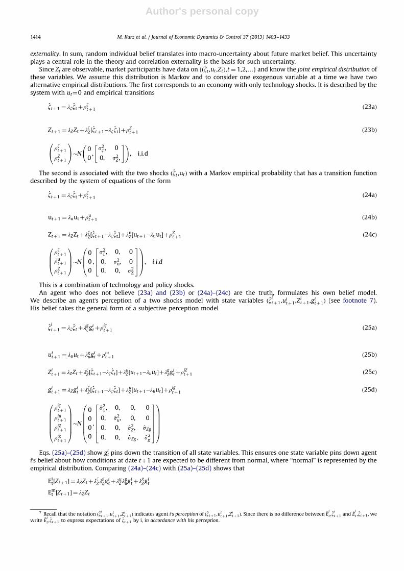
Since Zt are observable, market participants have data on fðζt ,ut ,ZtÞ,t ¼ 1,2,…g and know the joint empirical distribution ofthese variables. We assume this distribution is Markov and to consider one exogenous variable at a time we have twoalternative empirical distributions. The first corresponds to an economy with only technology shocks. It is described by thesystem with ut¼0 and empirical transitions
ζtþ1 ¼ λζζtþρζtþ1 ð23aÞ
Ztþ1 ¼ λZZtþλζZ ½ζtþ1−λζζt�þρZtþ1 ð23bÞ
ρζtþ1
ρZtþ1
0@
1A∼N
00,
s2ζ , 0
0, s2Z ,
" # !, i:i:d
The second is associated with the two shocks ðζt ,utÞ with a Markov empirical probability that has a transition functiondescribed by the system of equations of the form
ζtþ1 ¼ λζζtþρζtþ1 ð24aÞ
utþ1 ¼ λuutþρutþ1 ð24bÞ
Ztþ1 ¼ λZZtþλζZ½ζtþ1−λζζt�þλuZ½utþ1−λuut�þρZtþ1 ð24cÞ
ρζtþ1
ρutþ1
ρZtþ1
0BB@
1CCA∼N
000,
s2ζ , 0, 0
0, s2u, 00, 0, s2Z
2664
3775
0BB@
1CCA, i:i:d
This is a combination of technology and policy shocks.An agent who does not believe (23a) and (23b) or (24a)–(24c) are the truth, formulates his own belief model.
We describe an agent's perception of a two shocks model with state variables ðζitþ1,uitþ1,Z
itþ1,g
itþ1Þ (see footnote 7).
His belief takes the general form of a subjective perception model
ζitþ1 ¼ λζζtþλgζg
itþρiζtþ1 ð25aÞ
uitþ1 ¼ λuutþλgug
itþρiutþ1 ð25bÞ
Zitþ1 ¼ λZZtþλζZ ½ζtþ1−λζζt �þλuZ ½utþ1−λuut �þλgZg
itþρiZtþ1 ð25cÞ
gitþ1 ¼ λZgitþλζZ ½ζtþ1−λζζt �þλuZ ½utþ1−λuut �þρigtþ1 ð25dÞ
ρiζtþ1
ρiutþ1
ρiZtþ1
ρigtþ1
0BBBBB@
1CCCCCA∼N
0000
,
s2ζ , 0, 0, 0
0, s2u, 0, 0
0, 0, s2Z , sZg
0, 0, sZg , s2g
2666664
3777775
0BBBBB@
1CCCCCA
Eqs. (25a)–(25d) show git pins down the transition of all state variables. This ensures one state variable pins down agenti's belief about how conditions at date tþ1 are expected to be different from normal, where “normal” is represented by theempirical distribution. Comparing (24a)–(24c) with (25a)–(25d) shows that
Eit½Ztþ1� ¼ λZZtþλζZλgζg
itþλuZλ
gug
itþλgZg
it
Emt ½Ztþ1� ¼ λZZt
7 Recall that the notation ðζitþ1 ,uitþ1 ,Z
itþ1Þ indicates agent i's perception of ðζtþ1 ,ui
tþ1 ,Zitþ1Þ. Since there is no difference between E
it ,ζ
itþ1 and E
it ,ζtþ1, we
write Eit ,ζtþ1 to express expectations of ζtþ1 by i, in accordance with his perception.
M. Kurz et al. / Journal of Economic Dynamics & Control 37 (2013) 1403–14331414
Author's personal copy
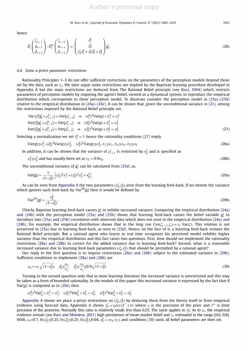
hence
Eit
ζtþ1
utþ1
Ztþ1
0B@
1CA−Emt
ζtþ1
utþ1
Ztþ1
0B@
1CA¼
λgζ
λguλζZλ
gζ þλuZλ
guþλgZ
0BB@
1CCAgit : ð26Þ
4.4. Some a-priori parameter restrictions
Rationality Principles 1–3 do not offer sufficient restrictions on the parameters of the perception models beyond thoseset by the data, such as λζ . We later argue some restrictions are implied by the Bayesian learning procedure developed inAppendix A but the main restrictions are deduced from The Rational Belief principle (see Kurz, 1994) which restrictsparameters of perception models by requiring the agent's belief, viewed as a dynamical system, to reproduce the empiricaldistribution which corresponds to these perception model. To illustrate consider the perception model in (25a)–(25d)relative to the empirical distribution in (24a)–(24c). It can be shown that, given the unconditional variance in (21), amongthe restrictions imposed by the Rational Belief principle are.
Var ½λgζgitþρiζtþ1� ¼ Var½ρζtþ1� ⇒ ðλgζ Þ2VarðgÞþ s2ζ ¼ s2ζ
Var½λgugitþρiutþ1� ¼ Var½ρutþ1� ⇒ ðλguÞ2VarðgÞþ s2u ¼ s2u
Var½λgZgitþρiZtþ1� ¼ Var½ρZtþ1� ⇒ ðλgZÞ2VarðgÞþ s2Z ¼ s2Z ð27Þ
Selecting a normalization we set λgζ ¼ 1 hence the rationality conditions (27) imply
VarðgÞ≤s2ζ , ðλguÞ2VarðgÞ≤s2u, ðλgZÞ2VarðgÞ≤s2Z , ~sζ≤sζ , ~su≤su, ~sZ≤sZ ð28aÞ
In addition, it can be shown that the variance of ρztþ1 is restricted by s2g and is specified as
s2Z≤s2g and has usually been set at sZ ¼ 0:9sg : ð28bÞ
The unconditional variance of git can be calculated from (25d) as.
Var g½ � ¼ 1ð1−λ2Z Þ
ðλζZ Þ2s2ζ þðλuZÞ2s2uþs2gh i
: ð29aÞ
As can be seen from Appendix A the two parameters ðλζZ ,λuZ Þ arise from the learning feed-back. If we denote the variancewhich ignores such feed-back by VarNF½g� then it would be defined by
VarNF g½ � ¼ s2gð1−λ2ZÞ
: ð29bÞ
Clearly, Bayesian learning feed-back causes git to exhibit increased variance. Comparing the empirical distribution (24a)and (24b) with the perception model (25a) and (25b) shows that learning feed-back causes the belief variable git tointroduce into (25a) and (25b) correlation with observed data which does not exist in the empirical distribution (24a) and(24b). For example, the empirical distribution shows that in the long run Covðζtþ1,ζtÞ ¼ λζ VarðζÞ. This relation is notpreserved in (25a) due to learning feed-back, as seen in (25d). Hence, on the face of it, a learning feed-back violates theRational Belief principle. But a rational agent who learns in real time recognizes his perceived model exhibits highervariance than the empirical distribution and this fact raises two questions. First, how should we implement the rationalityrestrictions (28a) and (28b) to correct for the added variance due to learning feed-back? Second, what is a reasonableincreased variance due to learning feed-back parameters ðλζZ ,λuZÞ that should be permitted by a rational agent?
Our reply to the first question is to impose restrictions (28a) and (28b) subject to the estimated variance in (29b).Sufficient conditions to implement (28a) and (28b) are
sg ¼ sζffiffiffiffiffiffiffiffiffiffiffiffiffiffið1−λ2ZÞ
q, λgu≤
susζ, λgZ≤
sZsζ≤0:9
ffiffiffiffiffiffiffiffiffiffiffiffiffiffið1−λ2ZÞ
qð30Þ
Turning to the second question note that in most learning literature the increased variance is unrestricted and this maybe taken as a form of bounded rationality. In the models of this paper this increased variance is expressed by the fact that ifVar(g) is computed as in (29a) then
ðλgζ Þ2Var2gþ s2ζ 4s2ζ , ðλguÞ2Var2gþ s2u4s2u, ðλgZÞ2Var2gþ s2Z4s2Z :
Appendix A shows we place a-priori restrictions on ðλζZ ,λuZÞ by deducing them from the theory itself or from empiricalevidence using forecast data. Appendix A shows λζZ ¼ ðμvÞ=ðΓ*þvÞ where ν is the precision of the prior and Γ* is limitprecision of the posterior. Normally this ratio is relatively small, less than 0.25. The same applies to λuZ . As to λz, the empiricalevidence reveals (see Kurz and Motolese, 2011) high persistence of mean market belief and λz estimated in the range [0.6, 0.8].With, λz≃0:7, 0≤λζZ≤0:25, 0≤λ
uZ≤0:25, 0≤λ
gZ≤0:64, λ
gu ¼ ðsu=sζÞ and conditions (30) used, all belief parameters are then set.
M. Kurz et al. / Journal of Economic Dynamics & Control 37 (2013) 1403–1433 1415
Author's personal copy
4.5. Definition of equilibrium
Having specified the belief of the agents, we define an equilibrium in the log-linearized economy.
Definition 2. Given a rule rt ¼ ξππtþξyytþut , an equilibrium in the log-linearized economy with two exogenous shocks is a
stochastic process fðrt ,pt ,πt ,wt ,ytÞ,t ¼ 1,2,…g and a collection of decision functions ðc jt ,b
j
t ,ℓjt ,n
jt ,y
jt ,q
*jtÞ such that:
(i) decision functions are optimal for all j given j's belief (25a)–(25d),(ii) markets clear:
R 10 cjtdj¼ yt ,
R 10 b
jt dj¼ 0, and
R 10 ℓ
jt dj¼
R 10 nj
t dj, and(iii) j's borrowing is bounded, transversality conditions satisfied and equilibrium is determinate.
Optimal decision functions ðc jt ,b
j
t ,ℓjt ,n
jt ,y
jt ,q
*jtÞ are linear in state variables but the issues at hand are the relevant state
variables. An equilibrium is said to be regular if it is expressed with finite state variables, a finite number of laggedendogenous variables and hence it is of finite memory. If xt is a finite vector of state variables in a regular equilibrium of thelog linearized economy then, as an equilibrium condition, an endogenous variable wt has a reduced form Awxt where Aw is avector of parameters. An equilibrium is irregular if it is not regular. In such equilibria endogenous variables depend on aninfinite number of lagged variables or on expectation over infinite number of forward looking variables which cannot bereduced to a finite set of past or present variables. Irregular equilibria are important but analytically more difficult tosimulate. This is of particular importance whenwe vary the monetary rule and consider later other rules which are differentfrom rt ¼ ξππtþξyytþut .
One uses standard dynamic programming to show that for the economy at hand equilibria leading to (16a)–(16c) withbeliefs (25a)–(25d) are regular. Individual decisions are functions of the state variables ðZt ,ζt ,ut ,b
j
t−1,gjtÞ while the
equilibrium map of the macro-variables ðrt ,pt ,πt ,wt ,ytÞ is stated, as a set of functions of the state variables ðZt ,ζt ,utÞ. Thedifference between state spaces relevant to each individual agent and state spaces relevant to the macro economy is animportant outcome of individual belief diversity.
Comment 4.1: comparison with the Arrow–Debreu's view of riskEquilibrium endogenous variables depend upon ðZt ,ζt ,utÞ and this highlights the fact that our equilibrium theory goes far
beyond the modeling of risk in an Arrow–Debreu economy. This fact was first explored in Kurz (1994), Kurz and Wu (1996)and Kurz (1997) who define the added uncertainty in our model as “Endogenous Uncertainty.” The essential point is that inan Arrow–Debreu economy the state space is defined only with respect to exogenous shocks while in our theory a centralsource of market risk is the future belief of agents. Since endogenous variables are functions of market belief and sinceagents need to forecast endogenous variables, they must forecast uncertain future market belief which, for each agent, is“the belief of others.” In the log linear economy the belief of others is defined by Zt and compared with an Arrow–Debreueconomy, our state space is expanded from ðζt ,utÞ to ðZt ,ζt ,utÞ. Since all three state variables are observed, there is noproblem of infinite regress and higher order beliefs. Market belief is observed and is thus common knowledge. All agentsform belief about future market belief in the way they form belief about any aggregate variable. Markets, however, areincomplete since data on belief (and on other variables such as unemployment) can only be collected by survey methods,making the data subject to errors in observation. Although such data is sufficient for economic analysis and decisions, it ishard to enforce contracts which are contingent upon information containing errors in measurement, a reason that maycause such contracts to be contested in court.
The expanded state space of our economy permits phenomena which an Arrow–Debreu economy does not permit. Theseare equilibrium movements which are volatile and “unexplainable” in the familiar way of pointing to exogenous shocks that“explain” events. Sudden shifts in belief distributions result in crashes of asset prices or dramatic moves of commodityprices. No technological or exogenous event can explain the 2007–2008 Financial Crisis but we do know that real estate andprivate housing portfolios were based on widely shared and correlated forecasts of ever rising real estate prices. Whenagents began to realize late in 2006 that these forecasts were highly correlated mistaken forecasts they first tried to unwindtheir leveraged positions. However, as expectations about future market belief shifted, asset prices began their long declineculminating in the financial crisis. These are exactly the phenomena captured by an equilibrium with endogenousuncertainty. No Black Swans or herding behavior with private information is needed to explain such events. All we need isfor individual agents to hold diverse but correlated beliefs and the conditions required for our theory to hold are simple:that agents hold common information, that this fact is common knowledge, that our economic environment is a complex,changing and non-stationary, and that in a changing environment agents can never learn the true economic structuregenerating the data. This collective ignorance is then common knowledge. Even when subjected to Rationality Axioms, roomis left for diverse models of deduction from available data, subjective but correlated interpretation of public signals availableto all (in the form of qualitative information) and persistence of diverse but correlated posterior estimates and forecasts.A central implication of our theory insists that holding a Rational belief and being wrong are not contradictory, and afinancial crisis can be ignited exactly by a large number of agents who commit substantial resources based on wrong andcorrelated forecasts. Indeed, the Rationality Axioms are exactly where one finds the formal route to explain the independentnature and persistence of the dynamics of belief, which is at the heart of the impact of expectations on market fluctuations.
M. Kurz et al. / Journal of Economic Dynamics & Control 37 (2013) 1403–14331416
Author's personal copy
We finally note this paper shows that, under the postulated beliefs, aggregation of equilibrium quantities is possible inthe log linearized economy. The paper also studies the impact of diverse beliefs on the performance of this log-linearizedeconomy. However, it is important to clarify the relationship between the microeconomic equilibrium of the log linearizedeconomy and the macroeconomic model implied by it. To understand why, recall that in a representative agent economy amacroeconomic model is a solution of a single agent's dynamic optimization. With diverse beliefs this is not true. Weexplain below that to define the macroeconomic model one must solve the log-linearized micro-equilibrium from which todeduce key parameters needed for the macro-model. Hence, changes in policy require a reconstruction of the macroeconomy and to that end one must re-solve the micro-equilibrium. In short, equilibrium of the log-linearized micro-economy remains a basic tool needed for the functioning of the macro-model!
5. Equilibrium of the log-linearized economy and the Effects of diverse Beliefs
A macro-model requires a solution of the problems arising from the terms ðΦtðcÞ,ΦtðqÞÞ and the mean forecast operatorEt ¼
R 10 Ejt dj: The following provides a general answer to these questions.
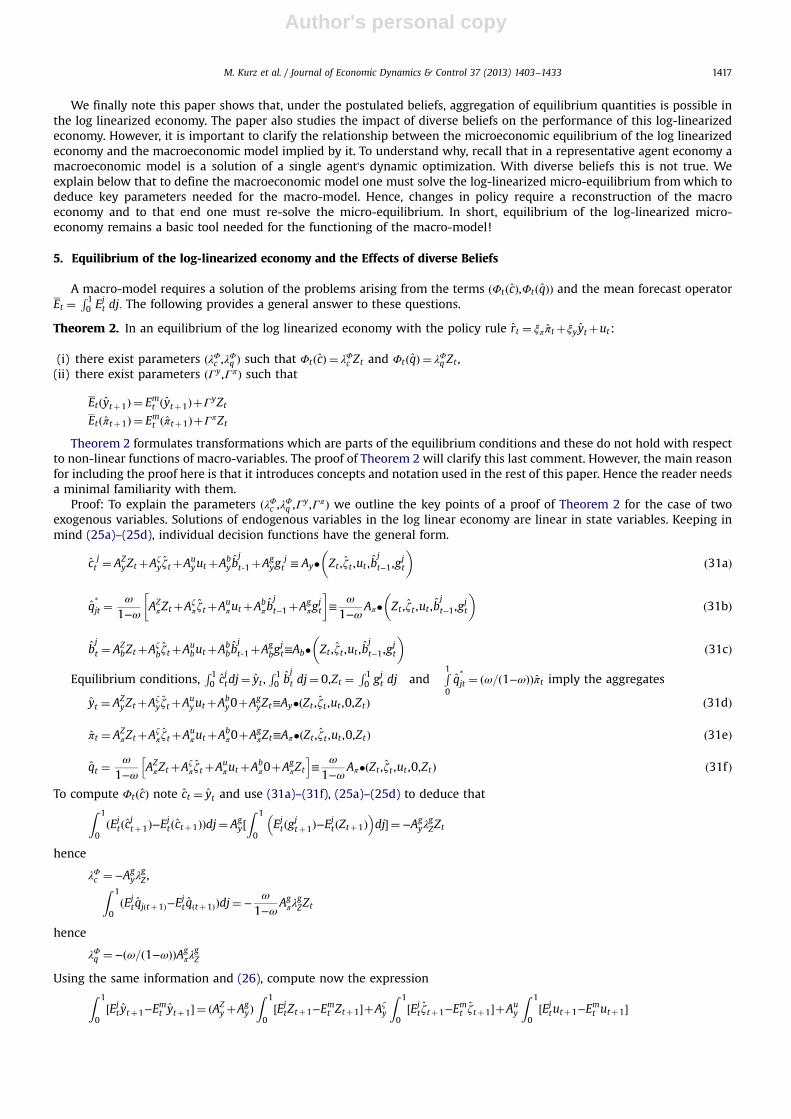
Theorem 2. In an equilibrium of the log linearized economy with the policy rule rt ¼ ξππtþξyytþut:
(i) there exist parameters ðλΦc ,λΦq Þ such that ΦtðcÞ ¼ λΦc Zt and ΦtðqÞ ¼ λΦq Zt ,(ii) there exist parameters ðΓy,ΓπÞ such that
Etðytþ1Þ ¼ Emt ðytþ1ÞþΓyZt
Etðπtþ1Þ ¼ Emt ðπtþ1ÞþΓπZt
Theorem 2 formulates transformations which are parts of the equilibrium conditions and these do not hold with respectto non-linear functions of macro-variables. The proof of Theorem 2 will clarify this last comment. However, the main reasonfor including the proof here is that it introduces concepts and notation used in the rest of this paper. Hence the reader needsa minimal familiarity with them.
Proof: To explain the parameters ðλΦc ,λΦq ,Γy,ΓπÞ we outline the key points of a proof of Theorem 2 for the case of twoexogenous variables. Solutions of endogenous variables in the log linear economy are linear in state variables. Keeping inmind (25a)–(25d), individual decision functions have the general form.
c jt ¼ AZ
yZtþAζyζtþAu
yutþAbyb
jt-1þAg
ygjt ≡ Ay�
�Zt ,ζt ,ut ,b
jt−1,g
jt
�ð31aÞ
q*jt ¼ω
1−ωAZπZtþAζ
π ζtþAuπutþAb
π bj
t−1þAgπg
jt
� �≡
ω
1−ωAπ� Zt ,ζt ,ut ,b
j
t−1,gjt
� �ð31bÞ
bjt ¼ AZ
bZtþAζbζtþAu
butþAbbb
jt-1þAg
bgjt≡Ab�
�Zt ,ζt ,ut ,b
jt−1,g
jt
�ð31cÞ
Equilibrium conditions,R 10 cjtdj¼ yt ,
R 10 b
j
t dj¼ 0,Zt ¼R 10 gjt dj and
R10q*jt ¼ ðω=ð1−ωÞÞπt imply the aggregates
yt ¼ AZyZtþAζ
yζtþAuyutþAb
y0þAgyZt≡Ay�ðZt ,ζt ,ut ,0,ZtÞ ð31dÞ
πt ¼ AZπZtþAζ
π ζtþAuπutþAb
π0þAgπZt≡Aπ�ðZt ,ζt ,ut ,0,ZtÞ ð31eÞ
qt ¼ω
1−ωAZπZtþAζ
π ζtþAuπutþAb
π0þAgπZt
h i≡
ω
1−ωAπ�ðZt ,ζt ,ut ,0,ZtÞ ð31f Þ
To compute ΦtðcÞ note ct ¼ yt and use (31a)–(31f), (25a)–(25d) to deduce thatZ 1
0ðEjtðcjtþ1Þ−Ejtðctþ1ÞÞdj¼ Ag
y½Z 1
0Ejtðgjtþ1Þ−EjtðZtþ1Þ� �
dj� ¼ −Agyλ
gZZt
hence
λΦc ¼−Agyλ
gZ ,Z 1
0ðEjt qjðtþ1Þ−E
jt qðtþ1ÞÞdj¼−
ω
1−ωAgπλ
gZZt
hence
λΦq ¼−ðω=ð1−ωÞÞAgπλ
gZ
Using the same information and (26), compute now the expressionZ 1
0½Ejt ytþ1−E
mt ytþ1� ¼ ðAZ
yþAgyÞZ 1
0½EjtZtþ1−Emt Ztþ1�þAζ
y
Z 1
0½Ejt ζtþ1−E
mt ζtþ1�þAu
y
Z 1
0½Ejtutþ1−Emt utþ1�
M. Kurz et al. / Journal of Economic Dynamics & Control 37 (2013) 1403–1433 1417
Author's personal copy
¼ ððAZyþAg
yÞ½λζZλgζ þλuZλguþλgZ �þAζ
yλgζ þAζ
yλguÞZt
Similar argument holds with respect to inflation hence we have that
Γy ¼ ðAZyþAg
yÞ½λζZλgζ þλuZλguþλgZ �þAζ
yλgζ þAu
yλgu ð31gÞ
Γπ ¼ ðAZπþAg
πÞ½λζZλgζ þλuZλguþλgZ �þAζ
πλgζ þAu
πλgu ð31hÞ
Note these transformations do not hold for, say ðytÞ2 which is not a linear function of state variables. □To study the systemwe transform it into one in which the expectation operator obeys the law of iterated expectations so
as to enable us to use standard techniques of analysis. To do that we observe that for defining the macro-model one needsonly the two parameters defined by
By ¼ λΦc þΓyþ 1s
� �Γπ , Bπ ¼ ð1−ωÞλΦq þΓπ :
Using the theorem above we can now rewrite system (16a)–(16c) in the form
IS curve yt ¼ Emt ðytþ1ÞþByZt �1s
� �rt−Emt ðπtþ1Þ� ð32aÞ
Phillips curve πt ¼ κðηþsÞytþβEmt πtþ1þβBπZt−κð1þηÞζt ð32bÞ
Monetary rule rt ¼ ξππtþξyytþut ð32cÞ
together with the law of motion of ðζt ,ut ,ZtÞ under the empirical transitions (24a)–(24c). Since this system is operative undera single probability law m which satisfies the law of iterated expectations, standard methods of Blanchard–Kahn (1980) areapplicable for setting conditions to ensure determinacy.
The system at hand shows that diverse beliefs have two effects. First, the mean market belief Zt has an amplificationeffect on the dynamics of the economy. The second is more subtle. To explain it note the probability in (32a) and (32b) is m,not the true dynamics (18a) and (18b) that is unknown to anyone and simulations are conducted with respect to theempirical probability m. Hence, (32a)–(32c) may not reflect changes in st (see (18a) and (18b)) if they are not predicted bythe public and expressed in Zt. But this fact shows that a central bank faces an enduring problem for which only imperfectsolutions exist. To capture what it does not observe, the bank has two options. One is to base policy upon market belief,expressed either directly by Zt or by asset prices which are functions of Zt (see Kurz and Motolese, 2011). A second option isto use the bank's own belief model in making policy decisions, giving rise to what the market would view as random policyshocks, which may turn out to be costly in becoming an independent cause of volatility. We return to this subject later whenwe discuss the implications to monetary policy.
5.1. Some characteristics of the microeconomic equilibrium
It follows from (31g) and (31h) that (By, Bπ) are functions of (Ay, Aπ, Ab) which is an equilibrium of the log-linearizedmicro-economy. That is, to deduce a solution of the macro-model (32a)–(32c), one must first obtain a micro-equilibriumsolution of (Ay, Aπ, Ab). Note that an equilibrium depends upon the model parameters including policy parameters. Since westudy the impact of changes in policy parameters, the shape of the map from parameters to equilibria (Ay, Aπ, Ab) isimportant. For this reasonwe use the term “EquilibriumManifold” to describe the set of equilibria (Ay, Aπ, Ab) as a function ofthe model's parameters.
Appendix B reviews computation of (Ay, Aπ, Ab) for a simple model of a technology shock with ut¼0. Exploring this modelfurther, note it is a system with endogenous variables ðπt ,ytÞ and shocks ðζt ,ZtÞ. Rewriting the system in a standard mannerwe have
ζtþ1 ¼ λζζtþρζtþ1 ð33aÞ
Ztþ1 ¼ λZZtþλζZ ½ζtþ1−λζζt �þρZtþ1 ð33bÞ
ρζtþ1
ρZtþ1
0@
1A∼N
00,
s2ζ ,sζZ
sζZ ,s2Z,
" # !
Emt ðytþ1Þ ¼ ytþ1s
� �ξππtþξyyt−E
mt ðπtþ1Þ
� −ByZt , By ¼ λΦc þΓyþ 1
s
� �Γπ ð33cÞ
Emt πtþ1 ¼1βπt−
κðηþsÞβ
yt−BπZt−1βκð1þηÞζt , Bπ ¼ ð1−ωÞλΦq þΓπ , κ¼ ð1−βωÞð1−ωÞ
ωð33dÞ
M. Kurz et al. / Journal of Economic Dynamics & Control 37 (2013) 1403–14331418
Author's personal copy
Eqs. (32a)–(32c) together with (33a)–(33d) show that endogenous variables do not affect the dynamics of either theexogenous shock or the dynamics of belief. It then follows that we have Proposition 3.
Proposition 3. Determinacy of equilibrium is not affected by diversity of beliefs.
Proof. It follows from Blanchard–Kahn (1980) that to compute the relevant eigenvalues one ignores the first two equations.For the case ut¼0, the condition for determinacy when ξy≥0, ξπ≥0 is
ξyð1−βÞþðξπ−1ÞκðηþsÞ40: ð34ÞIt does not involve belief parameters and is the same as an equivalent model with homogenous beliefs. □Does Proposition 3 mean that existence and uniqueness are the same as they would be without diverse beliefs?
The answer is No. To explain why, we continue to study the simple version of the model with a single exogenous technologyshock. We now explore some features of the equilibrium system.
Proposition 4. It is impossible to solve the macro-model using only the Macro-system (33a)–(33d). To solve (33a)–(33d) onemust first deduce (By, Bπ) from a micro-equilibrium of the log-linearized economy underlying (33a)–(33d).
Proof. See Appendix A □
Comment 5.1: interpretation of equilibrium; have we just created a new representative agent?This is an appropriate time to clarify what Theorem 2 says about the meaning of aggregation. After all, our starting point
is a diverse agent economy which we reduced to an economy where the aggregates follow their equilibrium path based onone probability measure, independently of the diversity with which we started. If diversity plays no role in the equilibriumpath, have we not created a new representative agent? We offer two answers. We first note that our methods andassumptions actually remove some effects of diversity but second, we explain why diversity is still at the heart of oureconomy.
By design, an equilibrium of a log linear economy disregards variances, focusing on mean values. In addition, thesampling Assumption 1 and Insurance Assumption 2 are designed to disregard income and distributional effects. It is thusno surprise that out of the diversity of beliefs represented by the distribution of git , all we find in the equilibrium of Theorem 2is only the mean Zt. Hence, our assumptions ensure that for any policy parameters, the dynamics of the aggregates in thelinearized economy do not depend upon time changes in the distribution of the heterogenous economy underneath theaggregates. This conclusion is in conflict with the empirical evidence of Kurz andMotolese (2011) who show that asset prices andexcess returns change in response to changes in the cross-sectional distribution of the git . It is thus clear that our model providesa first approximation inwhich some distributional effects on the aggregates have been assumed away. But then, if one is to arguethat Theorem 2 does not lead to a new representative agent economy, what is the role of belief diversity in the functioning ofthe model?
Our answer to the last question has two parts. One is formal and the second is a positive explanation of the role ofdiversity in the model's functioning. As to the formal part, since Zt is the mean belief, individual agents define their ownbeliefs relative to how they differ from Zt who, for each of them, reflects the belief of “others.” Hence, as a single agenteconomy the model in its present form loses its meaning. Under common knowledge of a single belief, agents know Zt ¼ githence they also know they do not need to forecast Zt≠git . Under such condition we must drop (22) and all transitions andperceptions like (23b), (24b) or (25c). With these changes the macro-system derived from Theorem 2 is not valid any longer.In short, without a background of belief diversity the model has no reasonable interpretation. By itself, Zt reflects beliefdiversity. A complimentary argument insists that the distinction between git and Zt results from the assumption of a non-stationary environment, which implies both the dynamics (21) of git and the belief diversity in the market. As long as weassume a non-stationary environment and deduce (21) we must also maintain a distinction between git and Zt. The fact thatwe reduced, via linearization and Assumptions 1 and 2, the causal impact of diversity on the aggregates does not mean thatthis needs to be the case in all future versions of the model. One important extension was proposed by Kurz and Motolese(2001) who show (p. 533) that changes in the cross-sectional distribution of the git changes the variance of Zt. To implementthis idea in our model recall that since the git in (21) are correlated, the random variable ~ρZtþ1 in (22) is the result ofaveraging (21), leading to the definition
limK→∞1K
∑K
i ¼ 1ρigtþ1 ¼ ~ρZtþ1:
The correlation across the ρigtþ1 is a belief externality, not subject to the rationality of any agent. Hence, it can exhibitcomplex behavior and the empirical distribution of ~ρZtþ1 does not need to have a constant variance s2Z , as assumed in (23b)above. Alternatively, ~ρZtþ1 can exhibit stochastic volatility, allowing the variance s2Z to be a function of the cross sectionalvariance of the ρigtþ1. There is substantial evidence for stochastic volatility in asset returns and in other macro economicvariables related to financial markets. The introduction of such stochastic volatility into our equilibrium would be a noveltyof its own.
Turning now to the positive explanation we suggest that our model is intended first of all to study the interactionbetween policy and market belief hence belief diversity plays an important role in two pivotal aspects of the model. First,diversity has an effect on the aggregates via its interaction with policy. Proposition 4 shows that in order to derive the
M. Kurz et al. / Journal of Economic Dynamics & Control 37 (2013) 1403–1433 1419
Author's personal copy
solution of the aggregates one must first compute the parameters ðBy,BπÞ, derived from the micro-equilibrium. Any changein policy changes the micro-equilibrium and hence ðBy,BπÞ. Second, since monetary policy is formulated as a function of theaggregates, the model aims to study how aggregates, via their impact on policy, affect the distribution and volatility of debtholdings and consumption. That is, instead of asking what is the effect of the distributions on the aggregates we suggest thatthe reverse question is very important. Hence, we question what is the effect of policy (and the resulting aggregates) on thedistribution and volatility of individual consumption and debt holdings. One of the important conclusions of this paper isthat the current exclusive focus on the aggregates is probably an error of policy. Belief diversity causes individualconsumption to be different from mean consumption which, in this model, equals output per capita. But if individualconsumption is different from per capita output then welfare considerations suggest that policy should be concerned withindividual consumption volatility at least as much as it is interested in the stability of the aggregates. In fact, policies thatstabilize the aggregates often cause high volatility of interest rates and financial markets, leading to volatile bond holdingand increased individual consumption volatility. In short, the fact that the economy is heterogenous remains a central factthat has an impact on the way we use the model for policy analysis and on the way we interpret its results. We now returnto exploring the characteristics of the micro-equilibrium.
Proposition 4 raises questions of existence and uniqueness of equilibria ðAy,Aπ ,AbÞ in the log linearized economy.The system of equations in the proof of Proposition 4 (Appendix A) implied by parameter matching is non-linear due to thepresence of products which arise from the borrowing function (Appendix A, Eqs. (A.8a)–(A.8c)). Indeed, there are 8 suchproducts: ðAb
yAzb;A
byA
ζb;A
byA
bb;A
byA
gbÞ and ðAb
πAZb ,A
bπA
ζb,A
bπA
bb,A
bπA
gbÞ. A close inspection leads to the following observation.
Proposition 5. The equation system defining equilibrium for τb40 is non-linear with at least two solutions where one entailsexplosive optimal borrowing (i.e. Ponzi ), independent of determinacy conditions.
Proof. See Appendix A. □
The dynamic determinacy condition (34) plays no role in Proposition 5. This fact suggests that determinacy conditionsrestrict the map which defines the micro-economic equilibrium only partly. This map can exhibit properties with importantconsequences (e.g. for individual borrowing patterns) which are not implied by dynamic determinacy. This, indeed, is theconclusion which is now explored.
5.2. Understanding equilibrium consequences of interactions of policy and beliefs
Selecting a non-explosive solution of Aby and Ab
π ¼ 0 proved in Proposition 5 reduces the system to six linear equations insix unknowns ðAy,AπÞ. Denote this equation system by MA¼f and inspection of (A.8a) and (A.8b) in Appendix A reveal thatterms included in the right hand vector f are only parameters of the exogenous shocks to the system. Hence, altering theseshocks impacts the equilibrium solution of A. But also, for a system without shocks f¼0, and there is no micro-economicequilibrium since belief variables are redundant: there is no equilibrium if one cannot define what beliefs are about.We refer to the determinant jMj as the “Equilibrium Determinant.” It helps understand the impact of diverse beliefs on policysince changes in policy parameters change the values of ðAy,Aπ ,AbÞ and ðBy,BπÞ in (33a)–(33d), and as we sweep over thefeasible space of policy parameters ðξy,ξπÞ the determinant changes. We know the basic fact that
Proposition 6. As one varies policy over the policy parameter space, the Equilibrium Determinant takes the value zero andchanges sign.
Note that Proposition 6 is not restricted to a determinacy region. As we sweep over feasible policies that satisfy determinacy(34), we sweep over the Equilibrium Manifold and raise two questions which are pivotal for the impact of policy on (sy,sπ):
(i) Do ðξy,ξπÞ have a monotonic effect on (sy, sπ) and what is the implied trade-off between them?(ii) Do ðξy,ξπÞ have a continuous effect on (sy, sπ)?
To resolve the question of continuity we later provide a simulation example to show the Equilibrium Determinant of aneconomy with diverse beliefs may take zero value and change sign inside the region of determinacy. This is not true forrational expectations under which determinacy excludes a zero determinant. Hence, the equilibrium map of an economywith diverse beliefs may have singularity inside the determinacy region when ðBy, BπÞ are unbounded and, by implication, insuch economy (sy, sπ) may not be continuous with respect to ðξy, ξπÞ within the region of determinacy. We now turn to thequestion of monotonicity.
To highlight the issues consider standard results of the RBC model (33a)–(33d) with ut ¼ 0 and RE under which all believe(24a) is the truth. Table 1.1 reports simulation results for ðξy≥0, ξπ≥1Þ which is the standard range used in most literature.8
8 Our model is quarterly but we report annualized statistics in all tables hence the inflation rate in the model is one quarter the rate reported in thetables. For consistency, the policy weight on output is also annualized in the table and hence in the simulations the rule would be defined asrt ¼ ξπ πtþðξy=4Þytþut .
M. Kurz et al. / Journal of Economic Dynamics & Control 37 (2013) 1403–14331420
Author's personal copy
The specified quarterly model parameters are standard (e.g. Galí, 2008; Woodford, 2003), and will be maintained throughout:
β¼ 0:99, s¼ 0:9, η¼ 1:0, τb ¼ 10−4, ω¼ 23, θ¼ 6, λζ ¼ 0:90
Assuming β¼ 0:99 means the riskless annualized rate is 4% which is compatible with the empirical record although wedo not aim here at exact calibration. The standard RBC assumption sζ ¼ 0:0072 of (measured for the “Solow Residuals”) isbeing used and we comment on this matter below. Also, recall that the empirical record for the US exhibits sy¼1.81,sπ¼1.79.
Table 1.1 shows that for sζ ¼ 0:0072 there are policy configurations for which the simulated values are within range ofthe data. More important is the effect of policy. The conclusions are as follows:
• Increasing ξy results in a monotonic decrease of sy and a monotonic increase of sπ .• Increasing ξπ results in a monotonic increase of syand a monotonic decrease of sπ .
These results imply a policy trade-off between sy and sπ , offering the central bank a choice between these volatilitymeasures. These results are consistent with the RE based model estimates of Taylor (1979), Fuhrer (1994), Ball (1999) andRudebusch and Svensson (1999) that imply such a trade-off. Although the steps of parameter change are wide, choice ofsmaller steps shows the results are continuous with respect to policy.
Why study monotonicity properties at all? There are two reasons for that. First, monotonic responses render the impactof policy predictable since it means a central bank knows the direction of an effect of increasing weight of a policyinstrument. In reality no central bank knows the exact effect of its instruments. Hence, a policy with non-monotonic effectsmeans a bank is uncertain not only about the size of the effect of policy but even about the direction of effects. This is anundesirable state of affairs.
A second reason for interest in the monotonic effects of ðξy,ξπÞ or other policy parameters is the one studied by Taylor(1979), Fuhrer (1994), Ball (1999), Rudebusch and Svensson (1999) and others who explored the policy trade-off between syand sπ . Monotonic response is a precondition for the policy trade-off exhibited by these authors for their models. Non-monotonic response may imply that a central bank does not have a policy trade-off between sy and sπ , a problem thatwould call for further examination.
Before proceeding we address the question of the size of the technological shock. The RBC approach assumedsζ ¼ 0:0072. Strong objections were raised against this measure and persuasive case was made in support of the viewthat much of this residual is not technology (e.g. Basu, 1996; Eichenbaum, 1991; King and Rebelo, 1999; Summers, 1986).Most scholars suggest it should be no more than sζ ¼ 0:004 hence we set sζ ¼ 0:004. Table 1.2 shows the well known factthat under RE with a single technology shock and sζ ¼ 0:004 the models’ business cycles volatility virtually disappears(see King and Rebelo, 1999). We will later show that when diverse beliefs are introduced, volatility is amplified andfluctuations contain a major component due to market belief. Under such conditions the model exhibits realistic volatilityand public stabilization policy of output and inflation becomes relevant. That is, central bank policy has an importantobjective of stabilizing the volatility amplification effect of market expectations!
6. An example: simulation results of the effects of diverse beliefs
6.1. Some preliminary Issues: determinacy Conditions and output difference vs. output gap
In this section we examine a two shock model with ut≠0 and a wider policy space which allows ðξyo0, ξπ≥1Þ.This implies that we need to revise the determinacy conditions. A condition ðξπo1Þ clearly violates determinacy. It followsfrom Proposition 1 of Bullard and Mitra (2002) that for determinacy to hold when ξyo0, condition (34) needs to besupplemented by the additional condition
ξyþκðηþsÞξπ4−ð1−βÞs: ð34aÞ
Table 1.1Annualized RBC Volatility and monotonicity under rational expectations. Standard RBC with sζ ¼ 0:0072.
sy ξy sp xy
0.0 0.6 1.2 1.5 30 0.0 0.6 1.2 1.5 30
ξπ 1.1 1.52 1.25 1.06 0.98 0.13 ξπ 1.1 2.74 5.98 8.24 9.12 19.251.6 1.68 1.57 1.47 1.43 0.38 1.6 0.86 2.15 3.28 3.80 16.302.2 1.71 1.65 1.59 1.56 0.59 2.2 0.47 1.22 1.91 2.24 13.772.8 1.72 1.68 1.64 1.62 0.75 2.8 0.33 0.85 1.34 1.58 11.9130 1.75 1.75 1.74 1.74 1.61 30 0.02 0.06 0.09 0.11 1.68
M. Kurz et al. / Journal of Economic Dynamics & Control 37 (2013) 1403–1433 1421
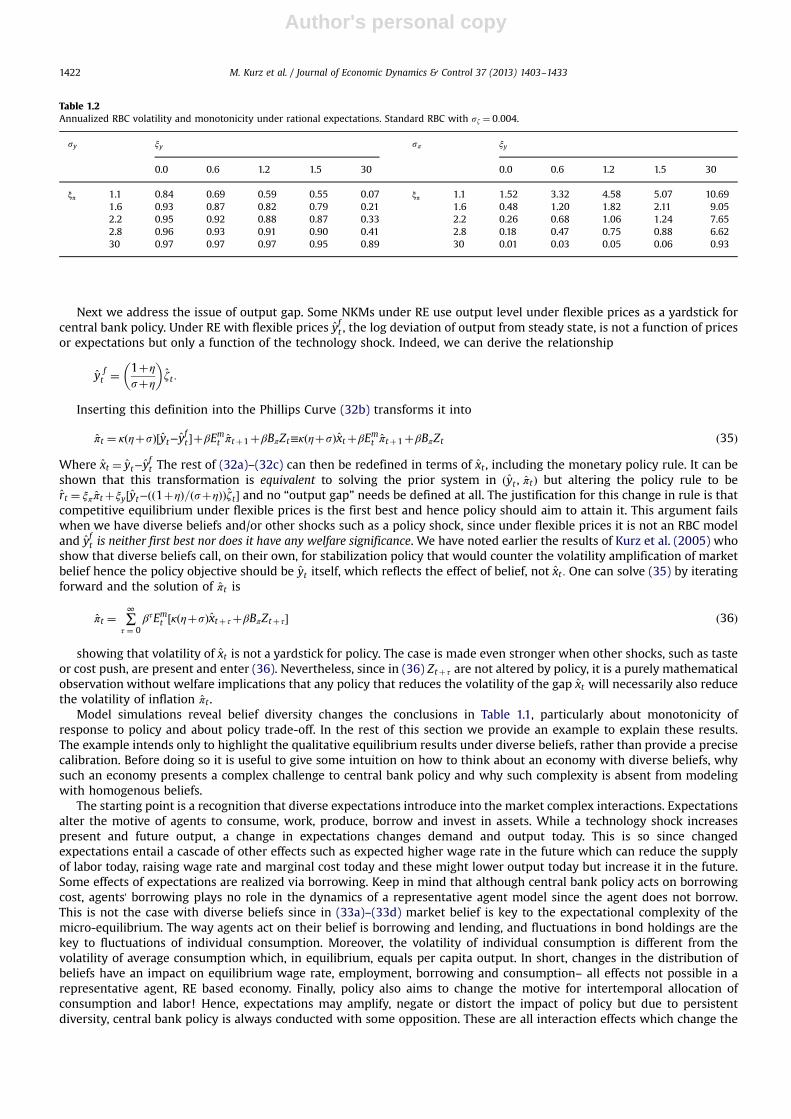
Author's personal copy
Next we address the issue of output gap. Some NKMs under RE use output level under flexible prices as a yardstick forcentral bank policy. Under RE with flexible prices yft , the log deviation of output from steady state, is not a function of pricesor expectations but only a function of the technology shock. Indeed, we can derive the relationship
y ft ¼ 1þη
sþη
� �ζt :
Inserting this definition into the Phillips Curve (32b) transforms it into
πt ¼ κðηþsÞ½yt−yft �þβEmt πtþ1þβBπZt≡κðηþsÞxtþβEmt πtþ1þβBπZt ð35Þ
Where xt ¼ yt−yft The rest of (32a)–(32c) can then be redefined in terms of xt , including the monetary policy rule. It can be
shown that this transformation is equivalent to solving the prior system in ðyt , πtÞ but altering the policy rule to bert ¼ ξππtþξy½yt−ðð1þηÞ=ðsþηÞÞζt � and no “output gap” needs be defined at all. The justification for this change in rule is thatcompetitive equilibrium under flexible prices is the first best and hence policy should aim to attain it. This argument failswhen we have diverse beliefs and/or other shocks such as a policy shock, since under flexible prices it is not an RBC modeland yft is neither first best nor does it have any welfare significance. We have noted earlier the results of Kurz et al. (2005) whoshow that diverse beliefs call, on their own, for stabilization policy that would counter the volatility amplification of marketbelief hence the policy objective should be yt itself, which reflects the effect of belief, not xt : One can solve (35) by iteratingforward and the solution of πt is
πt ¼ ∑∞
τ ¼ 0βτEmt ½κðηþsÞxtþ τþβBπZtþ τ� ð36Þ
showing that volatility of xt is not a yardstick for policy. The case is made even stronger when other shocks, such as tasteor cost push, are present and enter (36). Nevertheless, since in (36) Ztþ τ are not altered by policy, it is a purely mathematicalobservation without welfare implications that any policy that reduces the volatility of the gap xt will necessarily also reducethe volatility of inflation πt .
Model simulations reveal belief diversity changes the conclusions in Table 1.1, particularly about monotonicity ofresponse to policy and about policy trade-off. In the rest of this section we provide an example to explain these results.The example intends only to highlight the qualitative equilibrium results under diverse beliefs, rather than provide a precisecalibration. Before doing so it is useful to give some intuition on how to think about an economy with diverse beliefs, whysuch an economy presents a complex challenge to central bank policy and why such complexity is absent from modelingwith homogenous beliefs.
The starting point is a recognition that diverse expectations introduce into the market complex interactions. Expectationsalter the motive of agents to consume, work, produce, borrow and invest in assets. While a technology shock increasespresent and future output, a change in expectations changes demand and output today. This is so since changedexpectations entail a cascade of other effects such as expected higher wage rate in the future which can reduce the supplyof labor today, raising wage rate and marginal cost today and these might lower output today but increase it in the future.Some effects of expectations are realized via borrowing. Keep in mind that although central bank policy acts on borrowingcost, agents' borrowing plays no role in the dynamics of a representative agent model since the agent does not borrow.This is not the case with diverse beliefs since in (33a)–(33d) market belief is key to the expectational complexity of themicro-equilibrium. The way agents act on their belief is borrowing and lending, and fluctuations in bond holdings are thekey to fluctuations of individual consumption. Moreover, the volatility of individual consumption is different from thevolatility of average consumption which, in equilibrium, equals per capita output. In short, changes in the distribution ofbeliefs have an impact on equilibrium wage rate, employment, borrowing and consumption– all effects not possible in arepresentative agent, RE based economy. Finally, policy also aims to change the motive for intertemporal allocation ofconsumption and labor! Hence, expectations may amplify, negate or distort the impact of policy but due to persistentdiversity, central bank policy is always conducted with some opposition. These are all interaction effects which change the
Table 1.2Annualized RBC volatility and monotonicity under rational expectations. Standard RBC with sζ ¼ 0:004.
sy ξy sπ ξy
0.0 0.6 1.2 1.5 30 0.0 0.6 1.2 1.5 30
ξπ 1.1 0.84 0.69 0.59 0.55 0.07 ξπ 1.1 1.52 3.32 4.58 5.07 10.691.6 0.93 0.87 0.82 0.79 0.21 1.6 0.48 1.20 1.82 2.11 9.052.2 0.95 0.92 0.88 0.87 0.33 2.2 0.26 0.68 1.06 1.24 7.652.8 0.96 0.93 0.91 0.90 0.41 2.8 0.18 0.47 0.75 0.88 6.6230 0.97 0.97 0.97 0.95 0.89 30 0.01 0.03 0.05 0.06 0.93
M. Kurz et al. / Journal of Economic Dynamics & Control 37 (2013) 1403–14331422

Author's personal copy
simple picture in Table 1.1. The visible effect of diverse beliefs is seen in the fact that when policy parameters change, theequilibrium map changes, altering the parameters ðBy,BπÞ in (33a)–(33d) and hence ðsy,sπÞ.
6.2. The two shock ðζ,uÞ model (32a)–(32c) and individual consumption volatility
We allow ξyo0 as long as determinacy holds. Next, Table 2 provides results of simulating the diverse belief model (32a)–(32c) with realistic belief parameter values, most of which were motivated earlier: λz ¼ 0:7,λu ¼ 0:7, λζz ¼ 0:25,λuz ¼ 0:25, λgz ¼ 0:2, λgζ ¼ 1, λgu ¼ 0:5, sζ ¼ 0:004, su ¼ 0:002, sg ¼ 0:003: The parameters λu ¼ 0:7, su ¼ 0:002 were estimatedusing quarterly data on policy choices by the Federal Reserve.
Tables 2.1–2.4 reveal a more complex pattern of non-monotonicity than under RE in Table 1.1 with several reversals inthe effect of policy. In each of the tables one notes that, confining discussion to the region of determinacy, there are threeregions which are delineated by either the darker ridge on the right or by the minimum (with respect to ξy) region on theleft. For example, in Region 1 defined for sπ in Table 2.2 by approximately [−0.2, 0], as ξy rises from −0.2 the volatility ofinflation declines. In Region 2, defined between the minimal points of sy and up to the “ridge” extending from ξy ¼ 0:6 toξy ¼ 30, output volatility rises. In Region 3, beyond the ridge to the right, the volatility declines again with ξy: The same threeRegions are defined for inflation and individual consumption but both the region of minimum volatility and the ridge ofmaximal volatility vary among the three variables. Observe that in Region 2 an aggressive output stabilization policy usinglarger values of ξy is self defeating since it increases the volatility of output rather than decrease it. For individualconsumption the curve of minimal sc (with respect to ξy) extends across Table 2.3.
Table 2.4 provides the example of changed sign of the Equilibrium Determinant we promised earlier. It is seen that themaximal “ridge” of output and inflation volatilities correspond exactly to the values of policy parameters for which thedeterminant changes sign. It is thus clear that the non-monotonicity phenomenon discussed here is associated with thebehavior of the determinant over the feasible policy space.
We dispose of Region 1 which is clearly inefficient; no policy would be selected there since all three volatilities fall in thatregion. The key differences are between Regions 2 and 3. Before examining policy differences between these last tworegions, consider the effect of increasing the value of ξπ on the three endogenous variables. This effect clearly depends uponξy: In Region 3 the effect of increased ξπ is to increase the volatility of output, inflation and individual consumption. In thatregion the policy maker selects ξπ small in the region of determinacy (say ξπ¼1.1) and employs ξy to stabilize the market.In Region 2 the effect of increasing ξπ is drastically different since
• it reduces the volatility of output,• it reduces the volatility of inflation, and• it reduces the volatility of individual consumption up to a minimum level, marked in Table 2.3 by italics and dark shading,showing there is a limit to benefits of aggressive anti-inflation policy.
The difference between Regions 2 and 3 is that in Region 2 stabilization of output and inflation is achieved by anaggressive anti-inflation policy according to which the central bank selects ξπ at the largest politically feasible value. Suchpolicy cannot reduce output volatility beyond a lower bound but can reduce inflation volatility down to zero. Region 3 ischaracterized by a central bank that aims to lower output volatility to a level which is lower than the lower bound in Region 2,since in Region 3 output volatility can be reduced to zero by an aggressive ξy policy.
We examined the economy of Table 2 also with a policy that targets the gap xt ¼ yt−yft , discussed in Section 6.1. We can
report that, as one would expect, the quantitative results are slightly different but the qualitative results regarding non-monotonicity and different regions of reaction to policy are the same.
Turning now to a comparison of Regions 2 and 3, observe that an aggressive anti-inflationary policy in Region 2 aims tocontrol volatility caused, in part, by market belief. The policy has two limitations. The first, which we have already noted, isthat it has a bounded effect on output volatility, as seen at the bottom of Table 2.1. As ξπ⇒∞, the value of sy is bounded awayfrom zero (0.98 in Table 2.1). To reduce output volatility below this bound, the policy must move to Region 3. In this regionaggressive output stabilization policy is effective and large values of ξy do suppress output volatility but at the cost of veryhigh volatility of inflation and individual consumption. This volatility is too high and we comment on it later. Confiningourselves, for the moment, to output and inflation, the tables show a limited trade-off between sy and sπ in the conventionalsense of being defined on a concave surface. Instead, in this model a trade-off between inflation and output volatilities takesplace by a choice between regions of the policy space which reflect choice between aggressive inflation stabilization inRegion 2 and output stabilization policies in Region 3. These are two different but efficient visions of central bank policy.More generally, a trade-off faced by a central bank in our economy is a complex choice over regions in Tables 2.1–2.3 ratherthan a smooth choice over a continuous surface.
The second limitation of an anti-inflationary policy in Region 2 is unique to heterogenous economies and does not existin a single agent economy: the volatility of financial markets and individual consumption. Table 2.3 reports the volatility ofindividual consumption sc: This volatility cannot be computed from the macro-model; it must be computed from themicroeconomic equilibrium in which individual agents are symmetric. These agents hold diverse beliefs and borrow or lendto act upon these beliefs. Monetary policy has an impact on their choices and fluctuating interest rates interact with private
M. Kurz et al. / Journal of Economic Dynamics & Control 37 (2013) 1403–1433 1423
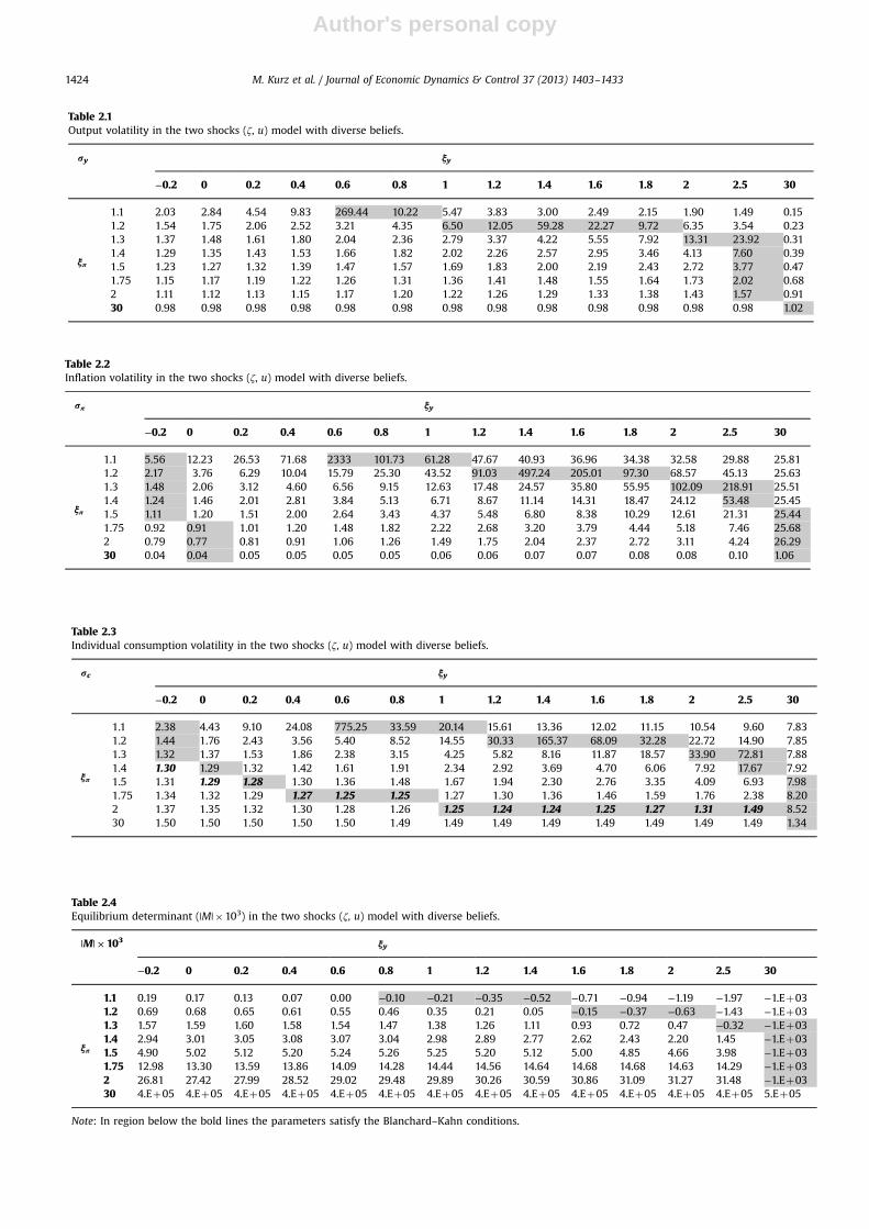
Author's personal copy
Table 2.4Equilibrium determinant (|M|�103) in the two shocks (ζ, u) model with diverse beliefs.
|M|�103 ξy
−0.2 0 0.2 0.4 0.6 0.8 1 1.2 1.4 1.6 1.8 2 2.5 30
ξπ
1.1 0.19 0.17 0.13 0.07 0.00 −0.10 −0.21 −0.35 −0.52 −0.71 −0.94 −1.19 −1.97 −1.Eþ031.2 0.69 0.68 0.65 0.61 0.55 0.46 0.35 0.21 0.05 −0.15 −0.37 −0.63 −1.43 −1.Eþ031.3 1.57 1.59 1.60 1.58 1.54 1.47 1.38 1.26 1.11 0.93 0.72 0.47 −0.32 −1.Eþ031.4 2.94 3.01 3.05 3.08 3.07 3.04 2.98 2.89 2.77 2.62 2.43 2.20 1.45 −1.Eþ031.5 4.90 5.02 5.12 5.20 5.24 5.26 5.25 5.20 5.12 5.00 4.85 4.66 3.98 −1.Eþ031.75 12.98 13.30 13.59 13.86 14.09 14.28 14.44 14.56 14.64 14.68 14.68 14.63 14.29 −1.Eþ032 26.81 27.42 27.99 28.52 29.02 29.48 29.89 30.26 30.59 30.86 31.09 31.27 31.48 −1.Eþ0330 4.Eþ05 4.Eþ05 4.Eþ05 4.Eþ05 4.Eþ05 4.Eþ05 4.Eþ05 4.Eþ05 4.Eþ05 4.Eþ05 4.Eþ05 4.Eþ05 4.Eþ05 5.Eþ05
Note: In region below the bold lines the parameters satisfy the Blanchard–Kahn conditions.
Table 2.3Individual consumption volatility in the two shocks (ζ, u) model with diverse beliefs.
rc ξy
−0.2 0 0.2 0.4 0.6 0.8 1 1.2 1.4 1.6 1.8 2 2.5 30
ξπ
1.1 2.38 4.43 9.10 24.08 775.25 33.59 20.14 15.61 13.36 12.02 11.15 10.54 9.60 7.831.2 1.44 1.76 2.43 3.56 5.40 8.52 14.55 30.33 165.37 68.09 32.28 22.72 14.90 7.851.3 1.32 1.37 1.53 1.86 2.38 3.15 4.25 5.82 8.16 11.87 18.57 33.90 72.81 7.881.4 1.30 1.29 1.32 1.42 1.61 1.91 2.34 2.92 3.69 4.70 6.06 7.92 17.67 7.921.5 1.31 1.29 1.28 1.30 1.36 1.48 1.67 1.94 2.30 2.76 3.35 4.09 6.93 7.981.75 1.34 1.32 1.29 1.27 1.25 1.25 1.27 1.30 1.36 1.46 1.59 1.76 2.38 8.202 1.37 1.35 1.32 1.30 1.28 1.26 1.25 1.24 1.24 1.25 1.27 1.31 1.49 8.5230 1.50 1.50 1.50 1.50 1.50 1.49 1.49 1.49 1.49 1.49 1.49 1.49 1.49 1.34
Table 2.1Output volatility in the two shocks (ζ, u) model with diverse beliefs.
ry ξy
−0.2 0 0.2 0.4 0.6 0.8 1 1.2 1.4 1.6 1.8 2 2.5 30
ξπ
1.1 2.03 2.84 4.54 9.83 269.44 10.22 5.47 3.83 3.00 2.49 2.15 1.90 1.49 0.151.2 1.54 1.75 2.06 2.52 3.21 4.35 6.50 12.05 59.28 22.27 9.72 6.35 3.54 0.231.3 1.37 1.48 1.61 1.80 2.04 2.36 2.79 3.37 4.22 5.55 7.92 13.31 23.92 0.311.4 1.29 1.35 1.43 1.53 1.66 1.82 2.02 2.26 2.57 2.95 3.46 4.13 7.60 0.391.5 1.23 1.27 1.32 1.39 1.47 1.57 1.69 1.83 2.00 2.19 2.43 2.72 3.77 0.471.75 1.15 1.17 1.19 1.22 1.26 1.31 1.36 1.41 1.48 1.55 1.64 1.73 2.02 0.682 1.11 1.12 1.13 1.15 1.17 1.20 1.22 1.26 1.29 1.33 1.38 1.43 1.57 0.9130 0.98 0.98 0.98 0.98 0.98 0.98 0.98 0.98 0.98 0.98 0.98 0.98 0.98 1.02
Table 2.2Inflation volatility in the two shocks (ζ, u) model with diverse beliefs.
rπ ξy
−0.2 0 0.2 0.4 0.6 0.8 1 1.2 1.4 1.6 1.8 2 2.5 30
ξπ
1.1 5.56 12.23 26.53 71.68 2333 101.73 61.28 47.67 40.93 36.96 34.38 32.58 29.88 25.811.2 2.17 3.76 6.29 10.04 15.79 25.30 43.52 91.03 497.24 205.01 97.30 68.57 45.13 25.631.3 1.48 2.06 3.12 4.60 6.56 9.15 12.63 17.48 24.57 35.80 55.95 102.09 218.91 25.511.4 1.24 1.46 2.01 2.81 3.84 5.13 6.71 8.67 11.14 14.31 18.47 24.12 53.48 25.451.5 1.11 1.20 1.51 2.00 2.64 3.43 4.37 5.48 6.80 8.38 10.29 12.61 21.31 25.441.75 0.92 0.91 1.01 1.20 1.48 1.82 2.22 2.68 3.20 3.79 4.44 5.18 7.46 25.682 0.79 0.77 0.81 0.91 1.06 1.26 1.49 1.75 2.04 2.37 2.72 3.11 4.24 26.2930 0.04 0.04 0.05 0.05 0.05 0.05 0.06 0.06 0.07 0.07 0.08 0.08 0.10 1.06
M. Kurz et al. / Journal of Economic Dynamics & Control 37 (2013) 1403–14331424
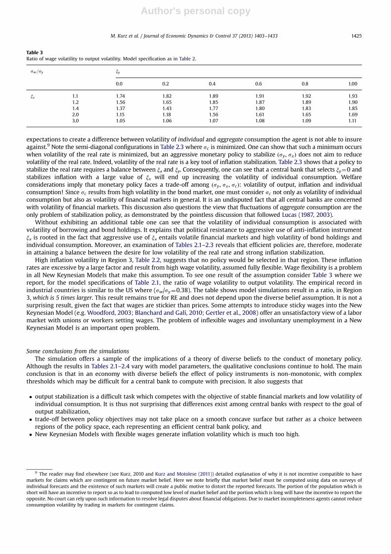
Author's personal copy
expectations to create a difference between volatility of individual and aggregate consumption the agent is not able to insureagainst.9 Note the semi-diagonal configurations in Table 2.3 where sc is minimized. One can show that such a minimum occurswhen volatility of the real rate is minimized, but an aggressive monetary policy to stabilize ðsy, sπÞ does not aim to reducevolatility of the real rate. Indeed, volatility of the real rate is a key tool of inflation stabilization. Table 2.3 shows that a policy tostabilize the real rate requires a balance between ξπ and ξy. Consequently, one can see that a central bank that selects ξy¼0 andstabilizes inflation with a large value of ξπ will end up increasing the volatility of individual consumption. Welfareconsiderations imply that monetary policy faces a trade-off among ðsy, sπ , scÞ: volatility of output, inflation and individualconsumption! Since sc results from high volatility in the bond market, one must consider sc not only as volatility of individualconsumption but also as volatility of financial markets in general. It is an undisputed fact that all central banks are concernedwith volatility of financial markets. This discussion also questions the view that fluctuations of aggregate consumption are theonly problem of stabilization policy, as demonstrated by the pointless discussion that followed Lucas (1987, 2003).
Without exhibiting an additional table one can see that the volatility of individual consumption is associated withvolatility of borrowing and bond holdings. It explains that political resistance to aggressive use of anti-inflation instrumentξπ is rooted in the fact that aggressive use of ξπ entails volatile financial markets and high volatility of bond holdings andindividual consumption. Moreover, an examination of Tables 2.1–2.3 reveals that efficient policies are, therefore, moderatein attaining a balance between the desire for low volatility of the real rate and strong inflation stabilization.
High inflation volatility in Region 3, Table 2.2, suggests that no policy would be selected in that region. These inflationrates are excessive by a large factor and result from high wage volatility, assumed fully flexible. Wage flexibility is a problemin all New Keynesian Models that make this assumption. To see one result of the assumption consider Table 3 where wereport, for the model specifications of Table 2.1, the ratio of wage volatility to output volatility. The empirical record inindustrial countries is similar to the US where (sw/sy¼0.38). The table shows model simulations result in a ratio, in Region3, which is 5 times larger. This result remains true for RE and does not depend upon the diverse belief assumption. It is not asurprising result, given the fact that wages are stickier than prices. Some attempts to introduce sticky wages into the NewKeynesian Model (e.g. Woodford, 2003; Blanchard and Galí, 2010; Gertler et al., 2008) offer an unsatisfactory view of a labormarket with unions or workers setting wages. The problem of inflexible wages and involuntary unemployment in a NewKeynesian Model is an important open problem.
Some conclusions from the simulationsThe simulation offers a sample of the implications of a theory of diverse beliefs to the conduct of monetary policy.
Although the results in Tables 2.1–2.4 vary with model parameters, the qualitative conclusions continue to hold. The mainconclusion is that in an economy with diverse beliefs the effect of policy instruments is non-monotonic, with complexthresholds which may be difficult for a central bank to compute with precision. It also suggests that
• output stabilization is a difficult task which competes with the objective of stable financial markets and low volatility ofindividual consumption. It is thus not surprising that differences exist among central banks with respect to the goal ofoutput stabilization,
• trade-off between policy objectives may not take place on a smooth concave surface but rather as a choice betweenregions of the policy space, each representing an efficient central bank policy, and
• New Keynesian Models with flexible wages generate inflation volatility which is much too high.
Table 3Ratio of wage volatility to output volatility. Model specification as in Table 2.
sw=sy ξy
0.0 0.2 0.4 0.6 0.8 1.00
ξπ 1.1 1.74 1.82 1.89 1.91 1.92 1.931.2 1.56 1.65 1.85 1.87 1.89 1.901.4 1.37 1.43 1.77 1.80 1.83 1.852.0 1.15 1.18 1.56 1.61 1.65 1.693.0 1.05 1.06 1.07 1.08 1.09 1.11
9 The reader may find elsewhere (see Kurz, 2010 and Kurz and Motolese (2011)) detailed explanation of why it is not incentive compatible to havemarkets for claims which are contingent on future market belief. Here we note briefly that market belief must be computed using data on surveys ofindividual forecasts and the existence of such markets will create a public motive to distort the reported forecasts. The portion of the population which isshort will have an incentive to report so as to lead to computed low level of market belief and the portion which is long will have the incentive to report theopposite. No court can rely upon such information to resolve legal disputes about financial obligations. Due to market incompleteness agents cannot reduceconsumption volatility by trading in markets for contingent claims.
M. Kurz et al. / Journal of Economic Dynamics & Control 37 (2013) 1403–1433 1425
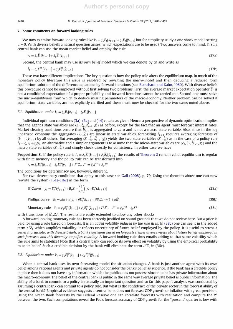
Author's personal copy
7. Some comments on forward looking rules
We now examine forward looking rules like rt ¼ ξπEt ½πtþ1�þξyEt ½ytþ1� but for simplicity study a one shock model, settingut¼0. With diverse beliefs a natural question arises: which expectations are to be used? Two answers come to mind. First, acentral bank can use the mean market belief and employ the rule
rt ¼ ξπEt ½πtþ1�þξyEt ½ytþ1� ð37aÞSecond, the central bank may use its own belief model which we can denote by cb and write as
rt ¼ ξπEcbt πtþ1� þξyE
cbt ½ytþ1� ð37bÞ
These two have different implications. The key question is how the policy rule alters the equilibrium map. In much of themonetary policy literature this issue is resolved by rewriting the macro-model and then deducing a reduced formequilibrium solution of the difference equations by forward iterations (see Blanchard and Kahn, 1980). With diverse beliefsthis procedure cannot be employed without first solving two problems. First, the average market expectation operator Et isnot a conditional expectation of a proper probability and forward iterations cannot be carried out. Second one must solvethe micro-equilibrium from which to deduce missing parameters of the macro-economy. Neither problem can be solved ifequilibrium state variables are not explicitly clarified and these must now be checked for the two cases noted above.
7.1. Equilibrium under rt ¼ ξπEt ½πtþ1�þξyEt ½ytþ1�
Individual optimum conditions (3a)–(3c) and (14) rt take as given. Hence, a perspective of dynamic optimization impliesthat the agent's state variables are ðZt , ζt , b
j
t−1, gjtÞ as before, except for the fact that an agent must forecast interest rates.
Market clearing conditions ensure that bj
t−1 is aggregated to zero and is not a macro-state variable. Also, since in the loglinearized economy the aggregates ðπt , ytÞ are linear in state variables, forecasting rtþ1 requires averaging forecasts ofðπtþ1, ytþ1Þ by all others. But averaging ðZt , ζt , b
j
t−1, gjtÞ yields the two state variables ðZt , ζtÞ as in the case of a policy rule
rt ¼ ξππtþξyyt . An alternative and a simpler argument is to assume that the micro-state variables are ðZt , ζt , bj
t−1, gjtÞ and the
macro state variables ðZt , ζtÞ and simply check directly for consistency. In either case we have
Proposition 8. If the policy rule is rt ¼ ξπEt ½πtþ1�þξyEt ½ytþ1� the results of Theorem 2 remain valid: equilibrium is regularwith finite memory and the policy rule can be transformed into
rt ¼ ξπEmt ½πtþ1�þξyE
mt ½ytþ1�þΓrZt , Γ
r ¼ ξyΓπþξyΓ
y
The conditions for determinacy are, however, different.For two determinacy conditions that apply to this case see Galí (2008), p. 79. Using the theorem above one can now
rewrite the system (16a)–(16c) in the form
IS Curve yt ¼ Emt ðytþ1ÞþByZt−1s
� �rt−Emt ðπtþ1Þ� ð38aÞ
Phillips curve πt ¼ κðηþsÞytþβEmt πtþ1þβBπZt−κð1þηÞζt ð38bÞ
Monetary rule rt ¼ ξπEmt ½πtþ1�þξyE
mt ½ytþ1�þΓrZt , Γr ¼ ξπΓ
πþξyΓy ð38cÞ
with transitions of ðζt ,ZtÞ. The results are easily extended to allow any other shocks.A forward looking monetary rule has been correctly justified on sound grounds that we do not review here. But a price is
paid for using a rule based on forecasts. It is an added volatility induced by the rule itself. In (38c) one can see it in the addedterm ΓrZt which amplifies volatility. It reflects uncertainty of future belief employed by the policy. It is useful to stress ageneral principle:with diverse beliefs, a bank's decisions based on forecasts trigger diverse views about future beliefs employed insuch forecasts and this diversity amplifies volatility. A forward looking rule thus entails adding to that same volatility whichthe rule aims to stabilize! Note that a central bank can reduce its own effect on volatility by using the empirical probabilitym as its belief. Such a credible decision by the bank will eliminate the term ΓrZt in (36c).
7.2. Equilibrium under rt ¼ ξπEcbt ½πtþ1�þξyE
cbt ½ytþ1�
When a central bank uses its own forecasting model the situation changes. A bank is just another agent with its ownbelief among rational agents and private agents do not consider the bank's belief as superior. If the bank has a credible policyin place then it does not have any information which the public does not possess since no one has private information aboutthe macro-economy. The belief of the central bank is public in the same way average private belief is public information. Theability of a bank to commit to a policy is naturally an important question and so far this paper's analysis was conducted byassuming a central bank can commit to a policy rule. But what is the confidence of the private sector in the forecast ability ofthe central bank? Empirical evidence suggests a central bank does not forecast GDP growth or inflation with great precision.Using the Green Book forecasts by the Federal Reserve one can correlate forecasts with realization and compute the R2
between the two. Such computations reveal the Fed's forecast accuracy of GDP growth for the “present” quarter is low with
M. Kurz et al. / Journal of Economic Dynamics & Control 37 (2013) 1403–14331426
Author's personal copy
R2 of about 0.5. For longer horizons they are very unreliable with R2 of about 0.25 for one quarter and R2 that fall to around0.15 for horizons above 6 months. The standard errors of the forecasts are usually very large. Inflation is highly persistenthence forecasting it is much easier. Even here the typical R2 between forecasts and realization by the Fed is about 0.5 forhorizons longer than 6 months.
Two additional facts about the Fed forecasting may be mentioned. First, the Green Book forecasts are made by the FederalReserve staff and released five years later. If the aim is to inform the public about the Fed's views why are the forecastsreleased only five years later? Second, members of the open market committee make their own individual forecasts andthese are released with the committee's minutes. Examination of these reveals wide differences in forecasts of GDP growthand inflation among members even for relatively short horizons. With wide differences of forecasts within the Fed, anyofficial “Central Bank Forecast” can only be some sort of a compromise the nature of which will only trigger more marketspeculations. It is thus not surprising markets treat the Fed forecasts as just one more forecast made by just one more agent.An important agent, to be sure, but not different in structure from the belief of anyone else.
To model the central bank as an agent requires us to specify the belief index gtcb
of the central bank. Using the same logicas the private sector, one establishes the transition of gt
cbto be as in (25c) and express the belief model of the bank by
ðζcbtþ1,Zcbtþ1,g
cbtþ1Þ with transitions
ζcbtþ1 ¼ λζζtþλgcbζ gcbt þρcbζtþ1, ð39aÞ
Zcbtþ1 ¼ λZZtþλζZ ½ζtþ1−λζζt �þλgcbZ gcbt þρcbZtþ1, ð39bÞ
gcbtþ1 ¼ λZgcbt þλζZ ½ζtþ1−λζζt �þρcbgtþ1, ð39cÞ
ρcbζtþ1
ρcbZtþ1
ρcbgtþ1
0BBB@
1CCCA∼N
00,0
s2ζ , 0, 0
0, s2Z , sZg ,
0, sZg , s2g
2664
3775
0BB@
1CCA
and a normalization λgcbζ ¼ 1. Eq. (39c) is the empirical distribution of gtcb. Agents take gt
cbas a new and relevant state variable
hence agent j's vector of state variables becomes ðZt ,ζt ,bj
t−1,gjt ,g
cbt Þ. One then recognizes the profound effect of the new state
variable which triggers private sector speculations about its future evolution. That is, is it true that (37c) is the truetransition of gcbt ? With individual beliefs formed about future beliefs of the central bank, the belief structure of the privatesector is further complicated. In this case private belief change from (25a)–(25c) to a general form of perception by privateagent i
ζitþ1 ¼ λζζtþλgζg
itþρiζtþ1 ð40aÞ
Zitþ1 ¼ λZZtþλζZ ½ζtþ1−λζζt �þλgZg
itþρiZtþ1 ð40bÞ
gcbitþ1 ¼ λZgcbt þλζZ ½ζtþ1−λζζt �þλgcbgitþρcbgtþ1 ð40cÞ
gitþ1 ¼ λZgitþλζZ ½ζtþ1−λζζt �þρigtþ1 ð40dÞ
with a covariance matrix. In (40a)–(40d) a belief state gtiimpacts three perceived transitions of macro-state variables
ðζt ,Zt ,gcbt Þ taken exogenously by i. Both private agents and the central bank formulate belief about future business conditionsexpressed by values of ζtþ1. This triggers an expanded individual state space and belief about future market belief Ztþ1 andfuture central bank belief gcbtþ1 with parameters ðλgZ ,λgcbÞ. Note the general principle implied: an ambiguity about the futureleads to an expansion of the issues subject to diverse belief and further amplification of market volatility. By basing policy onits own belief, a central bank opens the door for the market to endogenously add a component of uncertainty which was notthere before.
Aggregation and market clearing conditions show that macro-state variables ðZt ,ζt ,gcbt Þ are. In this case an equilibriumwith the central bank as an agent becomes regular with finite memory hence using (37a)–(37c) one can compute the newpolicy rule as follows. First compute the differences
Ecbt ½πtþ1�−Emt ½πtþ1� ¼ ½ðAZπþAg
πÞλζZþAζπþAgcb
π λgcbZ �gcbt
Ecbt ½ytþ1�−Emt ½ytþ1� ¼ ½ðAZyþAg
yÞλζZþAζyþAgcb
y λgcbZ �gcbt :
Next, write the new policy rule for the linearized economy expressed in terms of the probability m
rt ¼ ξπEcbt ½πtþ1�þξyE
cbt ½ytþ1� ¼ ξπE
mt ½πtþ1�þξyE
mt ½ytþ1�þ½ξπΓπcbþξyΓ
ycb�gcbt ð41Þ
M. Kurz et al. / Journal of Economic Dynamics & Control 37 (2013) 1403–1433 1427
Author's personal copy
where
Γπcb ¼ ½ðAZπþAg
πÞλζZþAζπþAgcb
π λgcbZ �, Γycb ¼ ½ðAZyþAg
yÞλζZþAζyþAgcb
y λgcbZ �,
But recall that the equilibrium parameters ðAZπ ,A
gπ ,A
ζπ ,A
gcbπ ,AZ
y ,Agy ,A
ζy;A
gcby Þ depend upon the policy!
The conclusion we draw from (36a) to (36c) and (39) is that, in the case at hand, when the central bank's belief is Markovand the empirical probability m is Markov, the resulting equilibrium has the same analytical structure as (32a)–(32c).Different policies will surely exhibit different dynamic properties but the causal structure remains the same: market beliefdoes not have an effect on determinacy, and Theorem 2 and Propositions 3 and 4 continue to hold. Since this macro systemhas different parameters the conditions for determinacy are different but employ the same formula (see Galí, (2008),page79).
Appendix A. Proofs of Theorem 1 and of Propositions 4 and 5
Proof of Theorem 1
Assumption 3. The alternate prior, based on the public signal, incorporates a direct learning process where
Sit∼N ψ it ,1γ
� �
One interpret ψ it as a prior subjective mean, positive or negative, given the qualitative public signal.
Proof. Using Assumption 3 combine the two sources to have that
Stðζt ,ψ itÞ ¼ μst−1ðζtÞþð1−μÞSit
with a mean of Eitðst ζt ,ψ itÞ ¼ μEitðst−1 ζtÞþð1−μÞψ i
t 0oμo1�����
and conditional variance Varðst jζt ,ψ itÞ ¼
μ2
ðαþνÞ þð1−μÞ2
γ
Let ξ1 ¼ ð1=μ2Þ and ξ2 ¼ ð1=ð1−μÞ2Þ and we write the precision of the distribution of this new posterior as
Precisionðst jζt ,ψ itÞ ¼ ΓðstÞ ¼ 1=
1ξ1ðαþνÞ þ
1ξ2γ
� �¼ ξ1ðαþνÞξ2γ
ξ1ðαþνÞþξ2γ
At date tþ1 the agent observes ζtþ1. By (18a) in the text in the form ζtþ1-λζζt ¼ stþεζtþ1, εζtþ1 �N 0, 1v
� it follows that
updating Eitðst jζt ,ψ itÞ the agent has
Eitþ1ðst jζtþ1,ψitÞ ¼
ΓðstÞEitðst jζt ,ψ itÞþν½ζtþ1�λζζt �
ΓðstÞþν,
stðζtþ1,ψitÞ∼N Eitðst jζtþ1,ψ
itÞ,
1ΓðstÞþν
� �:
After assessing the mean ψ itþ1 he formulates the new posterior which is
stþ1ðζtþ1,ψitþ1Þ ¼ μstðζtþ1,ψ
itÞþð1−μÞSitþ1
with mean
Eitþ1ðstþ1jζtþ1,ψitþ1Þ ¼ μEitþ1ðst jζtþ1,ψ
itÞþð1−μÞψ i
tþ1 0oμo1 ðA:1Þconditional variance
Varðstþ1jζtþ1,ψitþ1Þ ¼
1ξ1ðΓðstÞþνÞ þ
1ξ2γ
ðA:2Þ
and precision
Γðstþ1Þ ¼ 1=1
ξ1ðΓðstÞþνÞ þ1ξ2γ
� �¼ ξ1ðΓðstÞþνÞξ2γ
ξ1ðΓðstÞþνÞþξ2γðA:3Þ
We can now deduce the full symmetry of the process. For large t we then have
stðζtþ1,ψitÞ∼N Eitðst jζtþ1,ψ
itÞ,
1ΓðstÞþν
� �
Eitðst jζtþ1,ψitÞ ¼
ΓðstÞEitðst jζt ,ψ itÞþν½ζtþ1−λζζt �
ΓðstÞþν
M. Kurz et al. / Journal of Economic Dynamics & Control 37 (2013) 1403–14331428
Author's personal copy
After observing ψ itþ1 the new posterior is
stþ1ðζtþ1,ψitþ1Þ ¼ μstðζtþ1,ψ
itÞþð1−μÞSitþ1
The mean, conditional variance and precision are then as in (A1)–(A.3) and hence we have an equation for the precision
Γtþ1 ¼ξ1ðΓtþνÞξ2γξ1ðΓtþνÞþξ2γ
It is well defined for 1oξ1o∞ (i.e. 0oμo1) and in that case it has the unique positive solution
ξ1 ¼1μ2
and ξ2 ¼1
ð1−μÞ2, Γ* ¼
ðνþξ2γð1−ð1=ξ1ÞÞÞþffiffiffiffiffiffiffiffiffiffiffiffiffiffiffiffiffiffiffiffiffiffiffiffiffiffiffiffiffiffiffiffiffiffiffiffiffiffiffiffiffiffiffiffiffiffiffiffiffiffiffiðνþξ2γð1−ð1=ξ1ÞÞÞ2þ4ν
q2
40
The negative root has no economic meaning. When ξ1 ¼ 1, ξ2 ¼∞ there is no solution, and Γt diverges for large t, whichis the classical case. Now insert Γ ¼ Γ* into the equations above to deduce that
Eitþ1ðstþ1jζtþ1,ψitþ1Þ ¼ μEitþ1ðst jζtþ1,ψ tÞþð1−μÞψ i
tþ1
hence
Eitþ1ðstþ1jζtþ1,ψitþ1Þ ¼ μ
Γ*Eitðst jζt ,ψ itÞþν½ζtþ1−λζζt �Γ*þν
þð1−μÞψ itþ1 ðA:4Þ
Now define
gitþ1 ¼ Eitþ1ðstþ1jζtþ1,ψitþ1Þ, λz ¼
μΓ*
Γ*þν40, λζz ¼
μν
Γ*þν40, ρigtþ1 ¼ ð1−μÞψ i
tþ1
Hence, the law of motion of gitþ1 is
gitþ1 ¼ λzgitþλζz ½ζtþ1−λζζt �þρigtþ1 □ ðA:5ÞSome comments: Aggregation implies an empirical distribution of the form
Ztþ1 ¼ λzZtþλζz ½ζtþ1−λζζt �þρztþ1 ðA:6Þand a belief of i in the mean belief of others is defined by
Zitþ1 ¼ λzZtþλζz ½ζtþ1−λζζt �þλgzg
itþρiztþ1
For simulations one uses expressions (A.5) and (A.6). General equilibrium computations are based on expectations of(A.5) and (A.6) which are
Eit gitþ1
� �¼ λzþλζz�
git
Eit Zitþ1
� �¼ λzZtþ λζzþλgz
� git
These are then used in the general equilibrium computations of (Ay, Aπ) In addition, we have thatZ 1
0Eit gitþ1
� �−Eit Zi
tþ1
� �h idt ¼ λgzZt ðA:7Þ
Proof of Proposition 4. It is explained in Appendix B that equilibrium values (Ay, Aπ, Ab) of the micro-model are deducedfrom the log-linearized Euler Eqs. (5a) and (14) which we write in the form
cjtþ1s
� �ξππtþξyyt� ¼ Ejt cjtþ1
� �þ 1
s
� �Ejt πtþ1ð Þþτbb
j
t
1−ωω
q*jt ¼−κð1þηÞζtþκðηþsÞytþβð1−ωÞEjt q*jðtþ1Þ þ πtþ1
h iBy (31a)–(31f) one writes these equations in the following linear form in j's expected values
Ay�ðZt ,ζt ,bj
t−1,gjtÞþ
ξπs
Aπ�ðZt ,ζt ,0,ZtÞh i
þ ξys
Ay�ðZt ,ζt ,0,ZtÞh i
¼ Ay� Ejt Ztþ1�
,Ejt ζtþ1
h i,b
j
t ,Ejt gjtþ1
h i� �þ 1
s
� �Aπ�ðEjt Ztþ1
� ,Ejt ζtþ1
h i,0,Ejt Ztþ1
� ÞþτbAb�ðZt ,ζt ,bj
t−1,gjtÞ ðA:8aÞ
Aπ�ðZt ,ζt ,bjt−1,g
jtÞþκðηþsÞAy�ðZt ,ζt ,0,ZtÞ�
¼�κð1þηÞζtþβωAπ�ðEjt ½Ztþ1�,Ejt ½ζtþ1�,bj
t ,Ejt ½gjtþ1�Þþβð1−ωÞAπ�ðEjt ½Ztþ1�,Ejt ½ζtþ1�,0,Ejt ½Ztþ1�Þ ðA:8bÞ
and expectations defined by
M. Kurz et al. / Journal of Economic Dynamics & Control 37 (2013) 1403–1433 1429
Author's personal copy
Ejt ½ζjtþ1� ¼ λζζtþλgζg
it
Ejt ½Ztþ1� ¼ λZZtþλζZgjtþλgZg
jt
Ejt ½gjtþ1� ¼ λzgjtþλζZg
jt
The 12 equilibrium function values (Ay, Aπ, Ab) are determined by matching coefficients of the four state variables acrossequations. Inserting the expectation values into (A.8a) and (A.8b) one obtains 8 equations in the 12 unknown equilibriumvalues. It is shown in Appendix B that the final four restrictions follow from the optimal borrowing function which isdeduced from the budget constraint of agent j. Under the insurance assumption, this equation is defined by
bj
t ¼1βbj
t−1þ 1þ θ−1θ
sη
� �ðyt−cjtÞ ðA:8cÞ
Return now to (31a)–(31d) and by matching coefficients one deduces that the final four restrictions are
Azb ¼ Ag
y 1þ θ−1θ
sη
� �, Aζ
b ¼ 0, Abb ¼
1β−Ab
y 1þ θ�1θ
sη
� �, Ag
b ¼−Agy 1þ θ−1
θ
sη
� �ðA:8dÞ
This procedure cannot be carried out for (31a)–(31d). Using (31d) and (31e) one can write it in a linear form, and even byusing the borrowing restriction (A.8c) one can deduce only eight equations in 12 unknowns. □
Proof. of Proposition 5
Matching parameters of the state variable bi
tþ1 in (A.8a) and (A.8b) leads to two non-linear equations
Abyð1−Ab
bÞ ¼ τbAbb ðA:9aÞ
Abπ ¼ βωAb
πAbb ðA:9bÞ
Now, Aby ¼ 0⇒Ab
b ¼ 0 due to (A.9a) and Abb ¼ ð1=βÞ40 due to (A.8d). This is a contradiction, hence Ab
y≠0 (A.8d) and (A.9a)imply that
Abb ¼
Aby
Abyþτb
¼ 1β−Ab
y 1þ θ−1θ
sη
� �hence Ab
y ¼1β−
Aby
Abyþτb
" #1
½1þððθ−1Þ=θÞðs=ηÞ� ðA:9cÞ
If Abπ≠0 it follows that Ab
b ¼ ð1=βωÞ which contradicts (A.9c) hence Abπ ¼ 0. This implies that
AbπA
zb ¼ 0, Ab
πAζb ¼ 0, Ab
πAgb ¼ 0
Now use (A.8d) and (A.9c) to deduce
AbyA
zb ¼
1β−
Aby
Abyþτb
" #Agy
AbyA
ζb ¼ 0
AbyA
gb ¼−
1β−
Aby
Abyþτb
" #Agy
Next, let Ξ ¼ 1þððθ−1Þ=θÞðs=ηÞ which is positive since θ41 Then, (A.9c) implies the equation.
ðAbyÞ2−
1Ξ
1−ββ
−τb� �
Aby−
τbβΞ
¼ 0
for which there are two exact solutions
Aby ¼
ð1ΞÞð1−ββ −τbÞ7ffiffiffiffiffiffiffiffiffiffiffiffiffiffiffiffiffiffiffiffiffiffiffiffiffiffiffiffiffiffiffiffiffiffiffiffiffi1Ξ2 ð1−ββ −τbÞ2þ4 τb
βΞ
q2
ðA:10Þ
one positive and one negative. Indeed, these are approximately
Aby≅
1Ξ
1−ββ
� �40, Ab
y≅−τb
j ffiffiffiffiffiffiβΞ
p j o0
To deduce equilibrium insert a solution of (A.10) into the six products. Eqs. (A.9a) and (A.9b) then imply six linearequations in the six parameters (Ay, Aπ). But two solutions of Ab
y imply two solutions for (Ay, Aπ, Ab). Since Aby measures the
effect of bond holdings on consumption, Abyo0 imply increased consumption and borrowing when in debt and this causes
individual debt to diverge for any τb. This second solution is thus not an equilibrium! For τb40 the only equilibrium is the oneimplied by Ab
y40 in (A.10). □
M. Kurz et al. / Journal of Economic Dynamics & Control 37 (2013) 1403–14331430
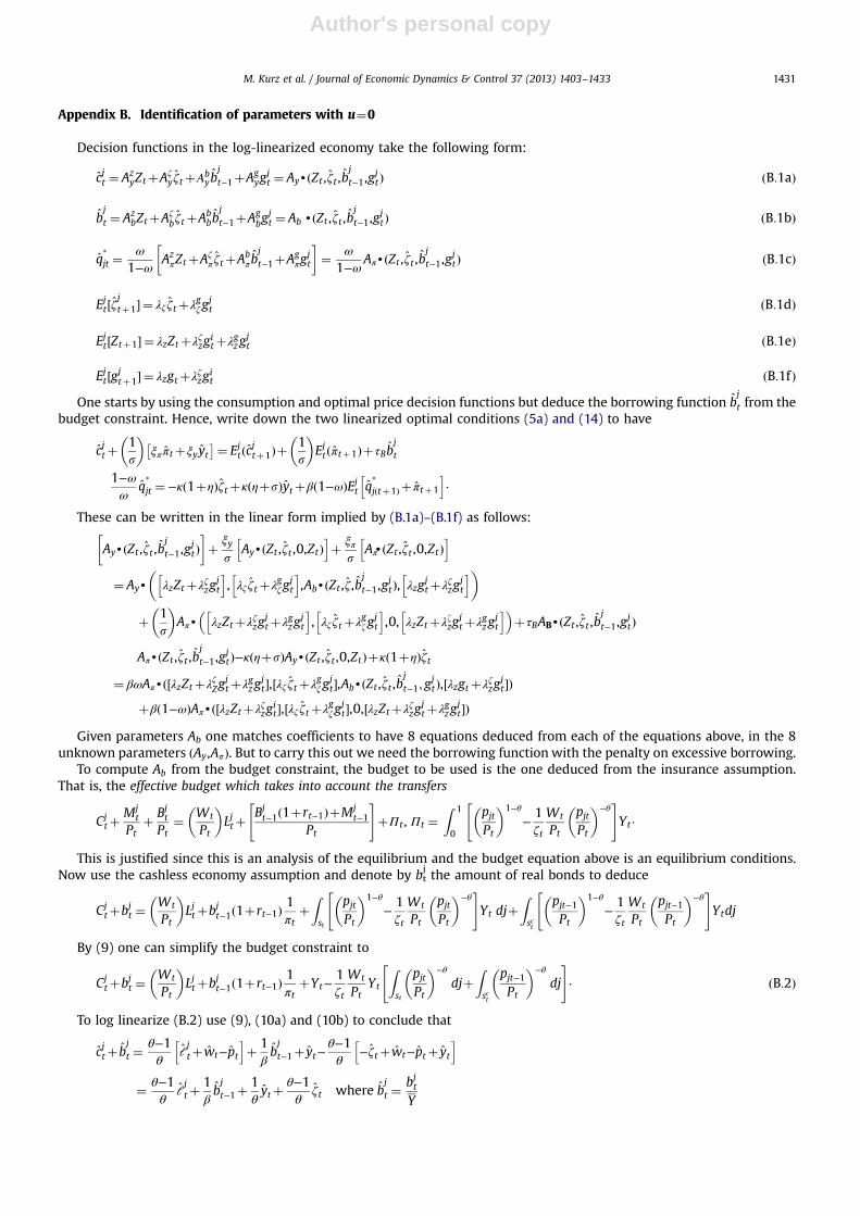
Author's personal copy
Appendix B. Identification of parameters with u¼0
Decision functions in the log-linearized economy take the following form:
cjt ¼ AzyZtþAζ
yζtþΑbyb
j
t−1þAgyg
jt ¼ AydðZt ,ζt ,b
j
t−1,gjtÞ ðB:1aÞ
bj
t ¼ AzbZtþAζ
bζtþAbbb
j
t−1þAgbg
jt ¼ Ab dðZt ,ζt ,b
j
t−1,gjtÞ ðB:1bÞ
q*jt ¼ω
1−ωAzπZtþAζ
π ζtþAbπ b
j
t−1þAgπg
jt
� �¼ ω
1−ωAπdðZt ,ζt ,b
j
t−1,gjtÞ ðB:1cÞ
Ejt ½ζjtþ1� ¼ λζζtþλgζg
jt ðB:1dÞ
Ejt ½Ztþ1� ¼ λzZtþλζzgitþλgzg
jt ðB:1eÞ
Ejt ½gjtþ1� ¼ λzgtþλζzgit ðB:1fÞ
One starts by using the consumption and optimal price decision functions but deduce the borrowing function bj
t from thebudget constraint. Hence, write down the two linearized optimal conditions (5a) and (14) to have
cjtþ1s
� �ξππtþξyyt� ¼ Ejtðcjtþ1Þþ
1s
� �Ejtðπtþ1ÞþτBb
j
t
1−ωω
q*jt ¼−κð1þηÞζtþκðηþsÞytþβð1−ωÞEjt q*jðtþ1Þ þ πtþ1
h i⋅
These can be written in the linear form implied by (B.1a)–(B.1f) as follows:
AydðZt ,ζt ,bj
t−1,gjtÞ
� �þ ξy
sAydðZt ,ζt ,0,ZtÞh i
þ ξπs
AπdðZt ,ζt ,0,ZtÞh i
¼ Ayd λzZtþλζzgjt
h i, λζζtþλgζg
jt
h i,AbdðZt ,ζ,b
j
t−1,gjtÞ, λzg
jtþλζzg
jt
h i� �
þ 1s
� �Aπd λzZtþλζzg
jtþλgzg
jt
h i, λζζtþλgzg
jt
h i,0, λzZtþλzzg
jtþλgzg
jt
h i� �þτBABdðZt ,ζt ,b
j
t−1,gjtÞ
AπdðZt ,ζt ,bj
t−1,gjtÞ−κðηþsÞAydðZt ,ζt ,0,ZtÞþκð1þηÞζt
¼ βωAπdð½λzZtþλζZgjtþλgzg
jt �,½λζζtþλgζg
jt �,AbdðZt ,ζt ,b
j
t−1; gjtÞ,½λzgtþλζzg
jt �Þ
þβð1−ωÞAπdð½λzZtþλζzgit �,½λζζtþλgζg
jt �,0,½λzZtþλζzg
jtþλgzg
jt �Þ
Given parameters Ab one matches coefficients to have 8 equations deduced from each of the equations above, in the 8unknown parameters ðAy,AπÞ. But to carry this out we need the borrowing function with the penalty on excessive borrowing.
To compute Ab from the budget constraint, the budget to be used is the one deduced from the insurance assumption.That is, the effective budget which takes into account the transfers
Cjtþ
Mjt
Ptþ Bj
t
Pt¼ Wt
Pt
� �Ljtþ
Bjt−1ð1þrt−1ÞþMj
t−1Pt
" #þΠt , Πt ¼
Z 1
0
pjtPt
� �1−θ
−1ζt
Wt
Pt
pjtPt
� �−θ" #
Yt ⋅
This is justified since this is an analysis of the equilibrium and the budget equation above is an equilibrium conditions.Now use the cashless economy assumption and denote by bt
jthe amount of real bonds to deduce
Cjtþbjt ¼
Wt
Pt
� �Ljtþbjt−1ð1þrt−1Þ
1πt
þZst
pjtPt
� �1−θ
−1ζt
Wt
Pt
pjtPt
� �−θ" #
Yt djþZsct
pjt−1Pt
� �1−θ
−1ζt
Wt
Pt
pjt−1Pt
� �−θ" #
Ytdj
By (9) one can simplify the budget constraint to
Cjtþbjt ¼
Wt
Pt
� �Ljtþbjt−1ð1þrt−1Þ
1πt
þYt−1ζt
Wt
PtYt
Zst
pjtPt
� �−θ
djþZsct
pjt−1Pt
� �−θ
dj
#⋅
"ðB:2Þ
To log linearize (B.2) use (9), (10a) and (10b) to conclude that
cjtþ bj
t ¼θ−1θ
ℓjtþwt−pt
h iþ 1
βbj
t−1þ yt−θ−1θ
−ζtþwt−ptþ yth i
¼ θ−1θ
ℓjtþ
1βbj
t−1þ1θytþ
θ−1θ
ζt where bj
t ¼bjtY
M. Kurz et al. / Journal of Economic Dynamics & Control 37 (2013) 1403–1433 1431
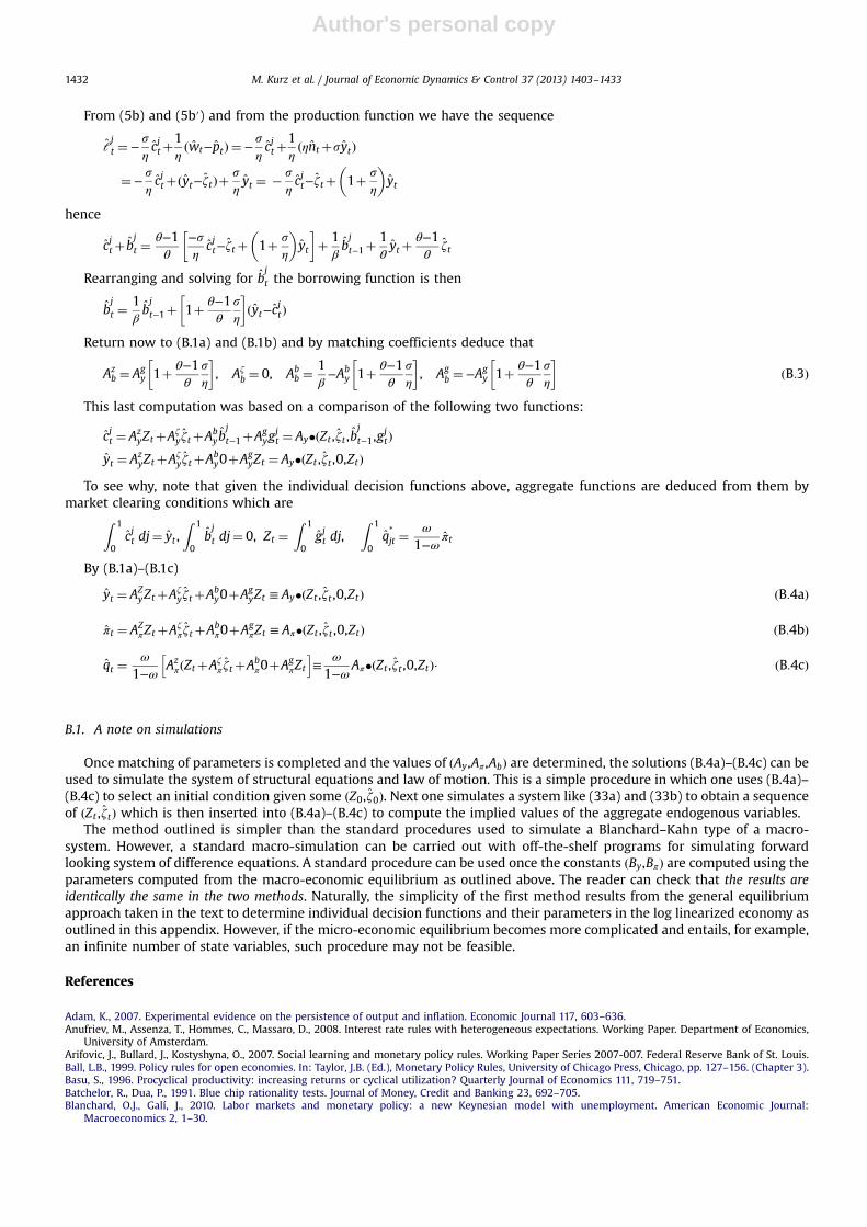
Author's personal copy
From (5b) and (5b′) and from the production function we have the sequence
ℓjt ¼−
sηcjtþ
1ηðwt−ptÞ ¼−
sηcjtþ
1ηðηntþsytÞ
¼−sηcjtþðyt−ζtÞþ
sηyt ¼ � s
ηcjt−ζtþ 1þ s
η
� �yt
hence
cjtþ bj
t ¼θ−1θ
−sη
cjt−ζtþ 1þ sη
� �yt
� �þ 1
βbj
t−1þ1θytþ
θ−1θ
ζt
Rearranging and solving for bjt the borrowing function is then
bj
t ¼1βbj
t−1þ 1þ θ−1θ
sη
� �ðyt−cjtÞ
Return now to (B.1a) and (B.1b) and by matching coefficients deduce that
Azb ¼ Ag
y 1þ θ−1θ
sη
� �, Aζ
b ¼ 0, Abb ¼
1β−Ab
y 1þ θ−1θ
sη
� �, Ag
b ¼−Agy 1þ θ−1
θ
sη
� �ðB:3Þ
This last computation was based on a comparison of the following two functions:
cjt ¼ AzyZtþAζ
yζtþAbyb
jt−1þAg
ygjt ¼ Ay�ðZt ,ζt ,b
jt−1,g
jtÞ
yt ¼ AzyZtþAζ
yζtþAby0þAg
yZt ¼ Ay�ðZt ,ζt ,0,ZtÞ
To see why, note that given the individual decision functions above, aggregate functions are deduced from them bymarket clearing conditions which areZ 1
0cjt dj¼ yt ,
Z 1
0bj
t dj¼ 0, Zt ¼Z 1
0gjt dj,
Z 1
0q*jt ¼
ω
1−ωπt
By (B.1a)–(B.1c)
yt ¼ AZyZtþAζ
yζtþAby0þAg
yZt ≡ Ay�ðZt ,ζt ,0,ZtÞ ðB:4aÞ
πt ¼ AZπZtþAζ
π ζtþAbπ0þAg
πZt ≡ Aπ�ðZt ,ζt ,0,ZtÞ ðB:4bÞ
qt ¼ω
1−ωAzπðZtþAζ
π ζtþAbπ0þAg
πZt
h i≡
ω
1−ωAπ�ðZt ,ζt ,0,ZtÞ⋅ ðB:4cÞ
B.1. A note on simulations
Once matching of parameters is completed and the values of ðAy,Aπ ,AbÞ are determined, the solutions (B.4a)–(B.4c) can beused to simulate the system of structural equations and law of motion. This is a simple procedure in which one uses (B.4a)–(B.4c) to select an initial condition given some ðZ0,ζ0Þ. Next one simulates a system like (33a) and (33b) to obtain a sequenceof ðZt ,ζtÞ which is then inserted into (B.4a)–(B.4c) to compute the implied values of the aggregate endogenous variables.
The method outlined is simpler than the standard procedures used to simulate a Blanchard–Kahn type of a macro-system. However, a standard macro-simulation can be carried out with off-the-shelf programs for simulating forwardlooking system of difference equations. A standard procedure can be used once the constants ðBy,BπÞ are computed using theparameters computed from the macro-economic equilibrium as outlined above. The reader can check that the results areidentically the same in the two methods. Naturally, the simplicity of the first method results from the general equilibriumapproach taken in the text to determine individual decision functions and their parameters in the log linearized economy asoutlined in this appendix. However, if the micro-economic equilibrium becomes more complicated and entails, for example,an infinite number of state variables, such procedure may not be feasible.
References
Adam, K., 2007. Experimental evidence on the persistence of output and inflation. Economic Journal 117, 603–636.Anufriev, M., Assenza, T., Hommes, C., Massaro, D., 2008. Interest rate rules with heterogeneous expectations. Working Paper. Department of Economics,
University of Amsterdam.Arifovic, J., Bullard, J., Kostyshyna, O., 2007. Social learning and monetary policy rules. Working Paper Series 2007-007. Federal Reserve Bank of St. Louis.Ball, L.B., 1999. Policy rules for open economies. In: Taylor, J.B. (Ed.), Monetary Policy Rules, University of Chicago Press, Chicago, pp. 127–156. (Chapter 3).Basu, S., 1996. Procyclical productivity: increasing returns or cyclical utilization? Quarterly Journal of Economics 111, 719–751.Batchelor, R., Dua, P., 1991. Blue chip rationality tests. Journal of Money, Credit and Banking 23, 692–705.Blanchard, O.J., Galí, J., 2010. Labor markets and monetary policy: a new Keynesian model with unemployment. American Economic Journal:
Macroeconomics 2, 1–30.
M. Kurz et al. / Journal of Economic Dynamics & Control 37 (2013) 1403–14331432

Author's personal copy
Blanchard, O.J., Kahn, C.M., 1980. The solution of linear difference models under rational expectations. Econometrica 48, 1305–1311.Branch, W.A., Evans, G.W., 2006. Intrinsic heterogeneity in expectation formation. Journal of Economic Theory 127, 264–295.Branch, W.A., Evans, G.W., 2011. Monetary policy with heterogeneous expectations. Economic Theory 47, 365–393.Branch, W.A., McGough, B., 2009. A new Keynesian model with heterogenous expectations. Journal of Economic Dynamics and Control 33, 1036–1051.Branch, W.A., McGough, B., 2011. Business cycle amplification with heterogenous expectations. Economic Theory 47, 395–421.Brazier, A., Harrison, R., King, M., Yates, T., 2008. The danger of inflating expectations of macroeconomic stability: heuristic switching in an overlapping
generations monetary model. International Journal of Central Banking 4, 219–254.Bullard, J., Mitra, K., 2002. Learning about monetary policy rules. Journal of Monetary Economics 49, 1005–1129.Calvo, G.A., 1983. Staggered prices in a utility maximizing framework. Journal of Monetary Economics 12, 983–998.De Grauwe, P., 2011. Animal spirits and monetary policy. Economic Theory 47, 423–457.Eichenbaum, M., 1991. Real business-cycle theory, wisdom or whimsy? Journal of Economic Dynamics and Control 15, 607–626.Evans, G., Honkapohja, S., 2003. Expectations and the stability problem for optimal monetary policies. Review of Economic Studies 70, 807–824.Evans, G., Honkapohja, S., 2006. Monetary policy, expectations and commitment. Scandinavian Journal of Economics 108 (1), 15–38.Frankel, J.A., Froot, K.A., 1990. Chartists, fundamentalists and the demand for dollars. In: Courakis, A.S., Taylor, M.P. (Eds.), Private Behavior and Government
Policy in Interdependent Economies, Oxford University Press, New York., pp. 73–126.Frankel, J.A., Rose, A.K., 1995. A survey of empirical research on nominal exchange rates. In: Grossman, G.M., Rogoff, K. (Eds.), Handbook of International
Economics III, North Holland, Amsterdam., pp. 1689–1729 (Chapter 33).Freedman, D., 1963. On the asymptotic behavior of bayes estimates in the discrete case I. Annals of Mathematical Statistics 34, 1386–1403.Freedman, D., 1965. On the asymptotic behavior of bayes estimates in the discrete case II. Annals of Mathematical Statistics 36, 454–456.Fuhrer, J.C., 1994. Optimal Monetary Policy and the Sacrifice Ratio. Boston Federal Reserve.Galí, J., 2008. Monetary Policy, Inflation and the Business Cycle: An Introduction to the New Keynesian Framework. Princeton University Press, Princeton.Gertler, M., Sala, L., Trigari, A., 2008. An estimated monetary DSGE model with unemployment and staggered nominal wage bargaining. Journal of Money,
Credit and Banking 40, 1713–1764.Howitt, P., 1992. Interest rate control and nonconvergence to rational expectations. Journal of Political Economy 100, 776–800.Jin, H., 2007. Nominal interest rate rules under heterogenous beliefs. Rivista Internazionale Di Scienze Sociali CXV 3, 403–442.Kandel, E., Pearson, N.D., 1995. Differential interpretation of public signals and trade in speculative markets. Journal of Political Economy 4, 831–872.King, R.G., Rebelo, S.T., 1999. Resuscitating real business cycles. In: Taylor, J., Woodford, M. (Eds.), Handbook of Macroeconomics, vol. 1B. , North-Holland,
Amsterdam., pp. 927–1007 (Chapter 14).Kurz, M., 1994. On the structure and diversity of rational beliefs. Economic Theory 4, 877–900 (an edited version appears as Chapter 2 of Kurz, M. (Ed.),
1997).Kurz, M. (Ed.), Studies in Economic Theory, vol. 6. , Springer-Verlag, Berlin, New York.Kurz, M., 2008. Beauty contests under private information and diverse beliefs: how different? Journal of Mathematical Economics 44, 762–784.Kurz, M., 2009. Rational diverse beliefs and economic volatility. In: Hens, T., Schenk-Hoppé, K.R. (Eds.), Handbook of Financial Markets: Dynamics
and Evolution, North-Holland, Amsterdam., pp. 440–506 (Chapter 8).Kurz, M., 2011. On the role of market belief in economic dynamics: an introduction. Economic Theory 47, 189–204.Kurz, M., 2012. A new Keynesian model with diverse beliefs. Working Paper. Stanford University, February 27, 2012.Kurz, M., Motolese, M., 2001. Endogenous uncertainty and market volatility. Economic Theory 17, 497–544.Kurz, M., Motolese, M., 2011. Diverse beliefs and time variability or risk premia. Economic Theory 47, 293–335.Kurz, M., Wu, H.M., 1996. Endogenous uncertainty in a general equilibrium model with price contingent contracts. Economic Theory 8, 461–488 (appears as
Chapter 2 of Kurz, M. (Ed.), 1997).Kurz, M., Jin, H., Motolese, M., 2005. The role of expectations in economic fluctuations and the efficacy of monetary policy. Journal of Economic Dynamics
and Control 29, 2017–2065.Lorenzoni, G., 2009. A theory of demand shocks. American Economic Review 99, 2050–2084.Lucas Jr., R.E., 1987. Models of Business Cycles. Basil Blackwell, New York Yrjö Jahnsson Lectures, Section III, pp. 20–31.Lucas Jr., R.E., 2003. Macroeconomic priorities. American Economic Review 4, 1–14.Massaro, D., 2012. Heterogeneous expectations in monetary DSGE models. Mimeo. University of Amsterdam.Milani, M., 2011. Expectation shocks and learning as drivers of the business cycle. Economic Journal 121, 379–401.Motolese, M., 2001. Money non-neutrality in a rational belief equilibrium with financial assets. Economic Theory 18, 97. 16.Motolese, M., 2003. Endogenous uncertainty and the non-neutrality of money. Economic Theory 21, 317–345.Rudebusch, G., Svensson, L.E.O., 1999. Policy rules for inflation targeting. In: Taylor, J.B. (Ed.), Monetary Policy Rules, University of Chicago Press, Chicago.,
pp. 203–262 (Chapter 5).Summers, L.H., 1986. Some skeptical observations on real business cycle theory. Federal Reserve Bank of Minneapolis Quarterly Review 10, 23–27.Takagi, S., 1991. Exchange rate expectations: a survey of survey studies. International Monetary Fund Staff Papers 38, 156–183.Taylor, B., 1979. Estimation and control of a macroeconomic model with rational expectations. Econometrica 47, 1267–1286.Walsh, C.E., 2010. Monetary Theory and Policy, Third edition The MIT Press, Massachusetts.Woodford, M., 2003. Interest and Prices: Foundations of a Theory of Monetary Policy. Princeton University Press, Princeton.Woodford, M., 2010. Robustly optimal monetary policy with near rational expectations. American Economic Review 100, 274–303.
M. Kurz et al. / Journal of Economic Dynamics & Control 37 (2013) 1403–1433 1433