Auto-B acklund Transformations and New Exact Travelling ... · description and the theoretical aspects of the model. The KP equation and its solitary answer are derived and described

Advanced Studies in Theoretical Physics

Vol. 8, 2014, no. 18, 789 - 810

HIKARI Ltd, www.m-hikari.com

http://dx.doi.org/10.12988/astp.2014.4797

Auto-Backlund Transformations and New Exact

Travelling Wave Solutions of Kadomtsev-Petviashvili

Equation for Nonlinear Dust Acoustic Solitary Waves

in Dust Plasmas with Variable Dust Charge and

Two Temperature Ions

R.S. Ibrahim1,a), A. R. Seadawy1,2 and H.A. Abd El-Hamed1

1 Mathematics Department, Faculty of Science

Beni-Suef University, Egypt

Mathematics Department, Faculty of Science

Taibah University, Al-Ula, Saudi Arabia

Copyright c© 2014 R.S. Ibrahim, A. R. Seadawy and H.A. Abd El-Hamed. This is an open access

article distributed under the Creative Commons Attribution License, which permits unrestricted use,

distribution, and reproduction in any medium, provided the original work is properly cited.

Abstract

The nonlinear dust acoustic solitary waves(DASWs) in two-dimensional dust

plasma with variable dust charge and two temperature ions has been studied an-

alytically. The Kadomtsev-Petviashvili equation (KP) equation for unmagnitized

dusty plasmas is derived by using the reductive perturbation theory. It suggests that

the nonlinear dust acoustic solitary waves with variable dust charge are stable even

there are some higher order transverse perturbations. We used the auto-Backlund

(BT) Transformation, the sine-cosine expansion method, the sinh-coshine expansion

method, the sech-tanh expansion method and the modified GG expansion method for

nonlinear partial differential equations(NPDEs) to obtained the new exact travelling

wave solutions of the KP equation describing the nonlinear DASWs in dust plasma.

790 R.S. Ibrahim, A. R. Seadawy and H.A. Abd El-Hamed

Keywords: dust plasma; KP equation, Reductive perturbation method, solitary

waves, Backlund transformations, Traveling wave solutions, Nonlinear partial differen-

tial equations

1 Introduction

The study of dusty plasmas represents one the most rapidly growing branches of plasma

physics. A dusty plasma is an ionized gas containing small particles of solid matter,

which acquire a large electric charge by collecting electrons and ions from the plasma.

Dust grains or particles are usually highly charged. Charged dust components appear

naturally in space environments such as planetary rings, cometary surroundings, inter-

stellar clouds, and lower parts of earths ionospheres [1-4]. The low frequency oscillations

in DASWs have been studied in [5-11]. Rao et al [12] first predicted theoretically the exis-

tence of extremely low phase velocity dust acoustic waves in unmagnetized dusty plasmas

whose constituents were inertial charged dust grains and Boltzmann-distributed ions and

electrons. These waves were reported experimentally and their nonlinear features investi-

gated by Barkar et al [13]. Due to their importance, the solitary waves in unmagnetized

plasma without geometry distortion and the dissipation effects have been extensively in-

vestigated and it was found that the solitary waves could be described by the Korteweg-de

Vries (KdV) equation or Kadomtsev-Petviashvili (KP) equation [14-16].

In the presented paper, the DASWs with variable dust charge and two temperature ions

has been considered. One can obtain the KP equation using the reductive perturbation

method on two dimensional unmagnetized case of this system. We would like to use the

homogeneous balance method [17,18] to constructed an auto-Backlund Transformation

(BT)[19-22] , new exact soliton solutions of KP equation are obtained and we have ap-

plied the sine-cosine expansion method, the sinh-coshine expansion method [23-26] , the

sech-tanh expansion method [24,27,28] and the modified GG

expansion method [29-35] to

obtained a new travelling wave solutions of KP equation.

The paper is organized as follows :This introduction in Section 1. In Section 2, the model

description and the theoretical aspects of the model. The KP equation and its solitary

answer are derived and described in this section. In section 3, the auto-Backlund Transfor-

mation (BT) applying to construct new exact soliton solutions of KP equation. In Section

4, the sine-cosine expansion method, the sinh-coshine expansion method, the sech-tanh

expansion method and the modified GG

expansion method are applied to construct new

travelling wave solutions of the KP equation. Finally, physical application of the solutions

are given in section 5. Conclusions are given in section 6.

Auto-Backlund transformations 791

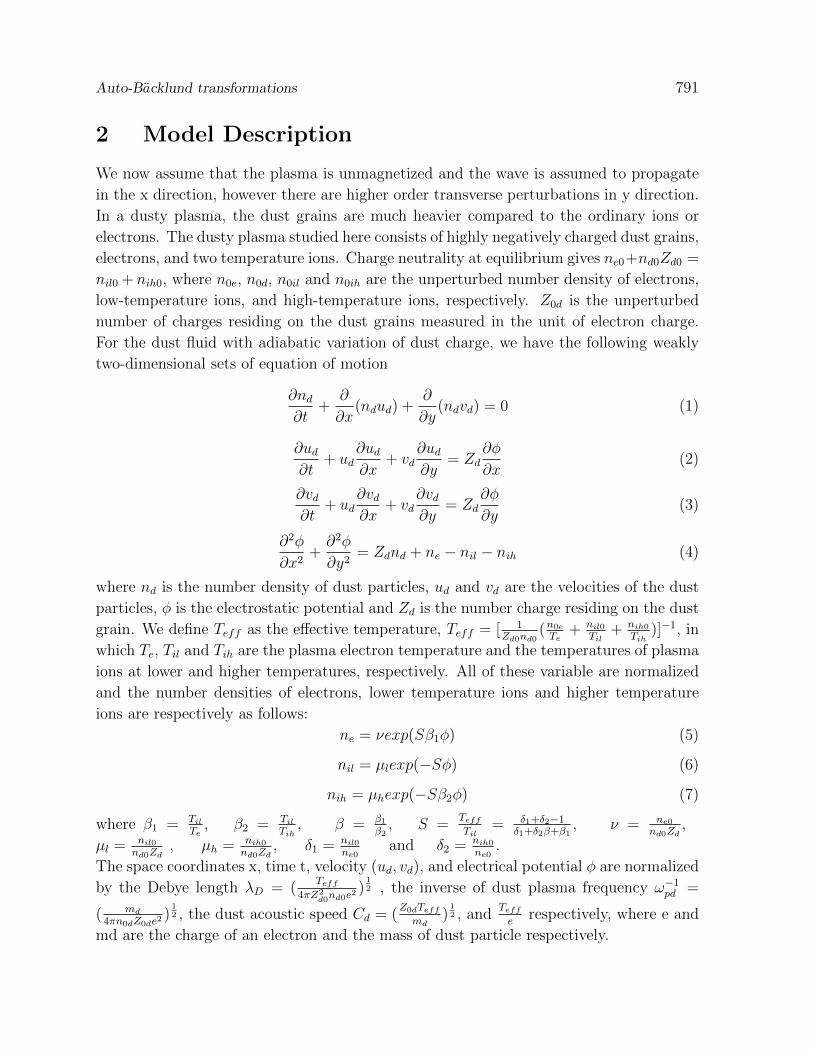
2 Model Description

We now assume that the plasma is unmagnetized and the wave is assumed to propagate

in the x direction, however there are higher order transverse perturbations in y direction.

In a dusty plasma, the dust grains are much heavier compared to the ordinary ions or

electrons. The dusty plasma studied here consists of highly negatively charged dust grains,

electrons, and two temperature ions. Charge neutrality at equilibrium gives ne0+nd0Zd0 =

nil0 + nih0, where n0e, n0d, n0il and n0ih are the unperturbed number density of electrons,

low-temperature ions, and high-temperature ions, respectively. Z0d is the unperturbed

number of charges residing on the dust grains measured in the unit of electron charge.

For the dust fluid with adiabatic variation of dust charge, we have the following weakly

two-dimensional sets of equation of motion

∂nd∂t

+∂

∂x(ndud) +

∂

∂y(ndvd) = 0 (1)

∂ud∂t

+ ud∂ud∂x

+ vd∂ud∂y

= Zd∂φ

∂x(2)

∂vd∂t

+ ud∂vd∂x

+ vd∂vd∂y

= Zd∂φ

∂y(3)

∂2φ

∂x2+∂2φ

∂y2= Zdnd + ne − nil − nih (4)

where nd is the number density of dust particles, ud and vd are the velocities of the dust

particles, φ is the electrostatic potential and Zd is the number charge residing on the dust

grain. We define Teff as the effective temperature, Teff = [ 1Zd0nd0

(n0e

Te+ nil0

Til+ nih0

Tih)]−1, in

which Te, Til and Tih are the plasma electron temperature and the temperatures of plasma

ions at lower and higher temperatures, respectively. All of these variable are normalized

and the number densities of electrons, lower temperature ions and higher temperature

ions are respectively as follows:

ne = νexp(Sβ1φ) (5)

nil = µlexp(−Sφ) (6)

nih = µhexp(−Sβ2φ) (7)

where β1 = TilTe

, β2 = TilTih

, β = β1β2

, S =TeffTil

= δ1+δ2−1δ1+δ2β+β1

, ν = ne0nd0Zd

,

µl = nil0nd0Zd

, µh = nih0nd0Zd

, δ1 = nil0ne0

and δ2 = nih0ne0

.

The space coordinates x, time t, velocity (ud, vd), and electrical potential φ are normalized

by the Debye length λD = (Teff

4πZ2d0nd0e

2 )12 , the inverse of dust plasma frequency ω−1

pd =

( md4πn0dZ0de2

)12 , the dust acoustic speed Cd = (

Z0dTeffmd

)12 , and

Teffe

respectively, where e and

md are the charge of an electron and the mass of dust particle respectively.


We now use the reductive perturbation method to obtain the Kadomtrev-Petriashvili

(KP) equation that governs the behavior of small amplitude dust acoustic waves. The

independent variables are stretched as

X = ε(x− v0t), T = ε3t, Y = ε2y (8)

where ε is a small dimensionless expansion parameter which characterizes the strength of

nonlinearity in the system and v0 is the phase velocity of the wave along the x direction.

We can expand physical quantities which have been appeared in (1-4) in term of the

expansion parameter ε as

nd = 1 + ε2n1 + ε4n2 + .... (9)

ud = ε2u1 + ε4u2 + .... (10)

vd = ε3v1 + ε5v2 + .... (11)

φ = ε2φ1 + ε4φ2 + .... (12)

Zd = 1 + ε2Z1 + ε4Z2 + .... (13)

where Z1 = γ1φ1, Z2 = γ1φ2 + γ2φ21 [36]

Substituting from equations (9-13)into equations (1-4). The KP equation is derived in

the form∂

∂X[∂φ1

∂T+ Aφ1

∂φ1

∂X+B

∂3φ1

∂X3] +D

∂2φ1

∂Y 2= 0 (14)

where

A =v3

0

2[(δ1 + δ2β

2 − β21)

δ1 + δ2 − 1

(δ1 + δ2β + β21)− 2γ2] +

3

2γ1v0 −

3

2v0

, B =v3

0

2, D =

v0

2(15)

3 Auto-Backlund Transformation (BT) and New Ex-

act Soliton Solutions of KP Equation.

By using the idea of the Homogeneous balance method [37], we seek for Backlund trans-

formation (BT) of KP equation (14) in the form

φ1(X, Y, T ) = ψ(Y, T )∂2Xf [ξ(X, Y, T ), η(X, Y, T )] + φ0(X, Y, T ), (16)

where ψ(Y, T ) is a differentiable function, f(ξ, η) is a function to be determined later and

φ0 be the special (old) solution of KP equation (14).

In the following analysis, we will stay with the following conditions

ψ(Y, T )) = 1, ηX(X, Y, T ) = 0⇒ η(X, Y, T ) = η(Y, T ) (17)

Substituting (16)and (17)into equation (14) yields


(Af 2ξξξ+Bfξξξξξξ+Afξξξξfξξ)ξ

6X+(ξXXXT+2AξXXXφ0X+BξXXXXXX+DξXXY Y +AξXXφ0XX

+AξXXXXφ0)fξ+(3ξXXξXT+3ξXξXXT+ξT ξXXX+6AξXξXXφ0X+15BξXXξXXXX+6BξXξXXXXX

+2Dξ2XY +2DξXξXY Y +10Bξ2

XXX+DξY Y ξXX+2DξY ξXXY +Aξ2Xφ0XX+3Aξ2

XXφ0+4AξXξXXXφ0)fξξ

+(3ξ2XξXT +3ξXξT ξXX +2Aξ3

Xφ0X +60BξXξXXξXXX +DξY Y ξ2X +4DξY ξXξXY +Dξ2

Y ξXX

+15Bξ2XξXXXX+15Bξ3

XX+6Aξ2XξXXφ0)fξξξ+(ξ3

XξT +45Bξ2Xξ

2XX+20Bξ3

XξXXX+Dξ2Y ξ

2X

+Aξ4Xφ0)fξξξξ+15Bξ4

XξXXfξξξξξ+12Aξ4XξXXfξξfξξξ+Aξ

4XξXXfξfξξξξ+(2AξXXXξ

3X+6Aξ2

Xξ2XX)fξfξξξ

+(12Aξ2Xξ

2XX + 4Aξ3

XξXXX)f 2ξξ + (10AξXξXXξXXX + Aξ2

XξXXXX + 3Aξ3XX)fξfξξ

+(Aξ2XXX+AξXXξXXXX)f 2

ξ +(ηT ξXXX+γξXXηY Y +2DηY ξXXY )fξη+(3ηT ξXξXX+4DηY ξXξXY

+2DξY ηY ξXX +DηY Y ξ2X)fξξη + (ξ3

XηT + 2DξY ηY ξ2X)fξξξη

+Dη2Y ξ

2Xfξξηη + φ0TX +Bφ0XXXX +Dφ0Y Y + Aφ0φ0XX + Aφ2

0X = 0 (18)

Setting the coefficients of ξ6X in (18) to zero, we obtain the ordinary differential equation

for f; namely

Af 2ξξξ +Bfξξξξξξ + Afξξξξfξξ = 0 (19)

which admits the solution

f = c ln(ξ) + ξσ(η) (20)

where σ(η) is differential function and c is arbitrary constant. According to (20), we

obtain

fξ =c

ξ+ σ, fξξ =

−cξ2, fξξξ =

2c

ξ3, fξξξξ =

−6c

ξ4, fξξξξξ =

24c

ξ5

, f 2ξξ =

−c6fξξξξ, f

2ξ =−1

c(c+ ξσ(η))2fξξ, fξfξξ =

−1

2(c+ ξσ(η))fξξξ,

fξfξξξ =−1

3(c+ ξσ(η))fξξξξ, fξξfξξξ =

−c12fξξξξξ, fξfξξξξ =

−1

4(c+ ξσ(η))fξξξξξ (21)

Substituting (19)and(21)into (18)yields a linear polynomial of fξ,fξξ,fξξξ, ... . Equating

the coefficients of fξ,fξξ,fξξξ, ... to zero, holds

ξXXXT + 2AξXXXφ0X +BξXXXXXX +DξXXY Y + AξXXφ0XX + AξXXXXφ0 = 0 (22)


3ξXXξXT + 3ξXξXXT + ξT ξXXX + 6AξXξXXφ0X + 15BξXXξXXXX + 6BξXξXXXXX

+2Dξ2XY + 2DξXξXY Y + 10Bξ2

XXX +DξY Y ξXX + 2DξY ξXXY + Aξ2Xφ0XX

+3Aξ2XXφ0 + 4AξXξXXXφ0 −

1

c(c+ ξσ(η))2(Aξ2

XXX + AξXXξXXXX) = 0 (23)

3ξ2XξXT + 3ξXξT ξXX + 2Aξ3

Xφ0X + 60BξXξXXξXXX +DξY Y ξ2X + 4DξY ξXξXY

+Dξ2Y ξXX + 15Bξ2

XξXXXX + 15Bξ3XX + 6Aξ2

XξXXφ0 −1

2(c+ ξσ(η))

(10AξXξXXξXXX + Aξ2XξXXXX + 3Aξ3

XX) = 0 (24)

ξ3XξT + 45Bξ2

Xξ2XX + 20Bξ3

XξXXX +Dξ2Y ξ

2X + Aξ4

Xφ0 −c

6(12Aξ2

Xξ2XX + 4Aξ3

XξXXX)

−1

3(c+ ξσ(η))(2AξXXXξ

3X + 6Aξ2

Xξ2XX) = 0 (25)

15Bξ4XξXX −

c

12(12Aξ4

XξXX)− 1

4(c+ ξσ(η))(Aξ4

XξXX) = 0 (26)

φ0TX +Bφ0XXXX +Dφ0Y Y + Aφ0φ0XX + Aφ20X = 0 (27)

The next crucial step is the assumption that

ξ(X, Y, T ) = 1 + expλ(T )±k1X±k2Y and φ0(X, Y, T ) = φ0 (28)

where k1 and k2 are arbitrary constants. Substituting into equations (22-27), results in

k1λ′(T ) +Bk4

1 +Dk22 + Aφ0k

21 = 0 (29)

7k1λ′(T ) + 31Bk4

1 + 7Dk22 + 7Aφ0k

21 −

2A

c(c+ ξσ(η))2(k4

1) = 0 (30)

6k1λ′(T ) + 90Bk4

1 + 6Dk22 + 6Aφ0k

21 − (c+ ξσ(η))(7Ak4

1) = 0 (31)

k1λ′(T ) +Dk2

2 + Aφ0k21 + (65B − 8

3Ac)k4

1 −8

3(c+ ξσ(η))(Ak4

1) = 0 (32)

60B − 5Ac− Aξσ(η) = 0 (33)

Solving the above system , we have

Case I.

λ =−Bk4

1 −Dk22 − Aφ0k

21

k1

T + c0, σ = 0, c =12B

A, (34)


where c0 is an integration constant, and let c0 = 0 . Substituting from equation (34) into

equation (28), we have

ξ(X, Y, T ) = 1 + exp−Bk41−Dk

22−Aφ0k

21

k1T±k1X±k2Y (35)

Substituting from equation (35) into equation (20), we have

f =12B

Aln(1 + exp

−Bk41−Dk22−Aφ0k

21

k1T±k1X±k2Y ) (36)

Substituting from equation (36) into equation (16), we get the new exact soltion solution

of KP equation (14) in the form

φ1 =6Bk2

1

A+ Acosh(Bk31T − k2Y +

Dk22T

k1+ k1(−X + Aφ0T ))

+ φ0 (37)

Case II.

λ =−Dk2

2

k1

T + c0, σ =−5(−2 + c)

ξ, (38)

where c0 is an integration constant, and let c0 = 0 . Substituting from equation (38) into

equation (28), we have

ξ(X, Y, T ) = 1 + exp−Dk22k1

T±k1X±k2Y (39)

Substituting from equation (39) into equation (20), we have

f = c ln(1 + exp−Dk22k1

T±k1X±k2Y )− 5(−2 + c) (40)

Substituting from equation (40) into equation (16), we have the new exact soltion solution

of KP equation (14) in the form

φ1 =ck2

1

2 + 2cosh(−Dk22Tk1

+ k1X + k2Y )+ φ0, (41)

under the condition

c =4(−2 + cosh(−Dk2

2T/k1 + k1X + k2Y ))(Bk22 + Ak2

1φ0)

(−4Ak41 + 5Ak4

1sech(1/2(−Dk22T/k1 + k1X + k2Y )2)

(42)


4 Travelling Wave solutions of the KP equation by

Applying the sine-cosine expansion method, the

sinh-coshine expansion method, the sech-tanh ex-

pansion method and the modified GG expansion method

4.1 The sine-cosine expansion method

Suppose that a nonlinear partial differential equation (NPDE) is given by

F (φ, φX , φY , φT , φXX , φY Y , φXY , φTT , .......) = 0. (43)

where φ = φ(X, Y, T ) is unknown function and F is a polynomial in and its partial

derivatives, in which the highest order derivatives and nonlinear terms are involved. In

the following we give the main steps of the sine-cosine expansion method:

Step 1.The traveling wave variable

φ(X, Y, T ) = φ(ξ), ξ = kX + lY − cT, (44)

where k, l and c are constants, permits us to reduce (43) into the following ordinary

differential equation (ODE);

F (φ, φ′, φ′′, φ′′′, .....) = 0. (45)

Step 2. Suppose that the solution of (45) can be expressed in the form as follows;

φ(ξ) = A0 +n∑i=1

cosi−1(w(ξ))[Aisin(w(ξ))] +Bicos(w(ξ))], (46)

whereAi (i = 0, 1, ...., n) and Bi (i =1, ...., n) are constants to be determined.

Step 3.The parameter ”n” in (46) can be found by balancing the highest order derivatives

term and the highest nonlinear term in (45);

(i)if n is a positive integer then go to step 4;

(ii)if n is not positive integer, we put φ = vn and then return to step 1.

Step 4. Substitute (46) with the fixed parameter n into the obtained ODE using

dω(ξ)

dξ= µ

√a+ bsin2ω(ξ), µ = ±1, (47)

where a and b are constants. collecting all terms with the same powers of w′ssiniwcosjw

together. Set to zero the coefficients of w′ssiniwcosjw(i = 0, 1; s = 0, 1; j = 0,1, 2,...,n)

to get a set of algebraic equations Cijs (AS, BS) = 0 with respect to the unknowns A0, c,


Ai(i = 1, ...., n) and Bi (i=1, ...., n).

Step 5.Solve the set of algebraic equations to get A0, Ai and Bi, then we have the

traveling wave solutions of the given nonlinear equation. In The sine-cosine expansion

method there are three cases of (35) :

Case I

In these case a=0, b=1, then the equation reduces to the first-order ODE

dw(ξ)

dξ= sin(w(ξ)), (48)

which has the solutions:

sin(w(ξ)) = sech(ξ), orcos(w(ξ)) = −tanh(ξ)

and sin(w(ξ)) = icsch(ξ), orcos(w(ξ)) = −coth(ξ),

where i =√−1

Case II

In these case a = 1, b = −m2, then the equation reduces to the first-order ODE

dw(ξ)

dξ= ±

√1−m2sin2(w(ξ)), (49)

where m is the modulus of Jacobi elliptic functions, which has the solutions

sin(w(ξ)) = sn(ξ;m), orcos(w(ξ)) = cn(ξ;m)

and sin(w(ξ)) = ns(ξ;m)m

, orcos(w(ξ)) = ids(ξ;m)m

Case III

In these case a = m2, b = −1, then the equation reduces to the first-order ODE,

dw(ξ)

dξ= ±

√m2 − sin2(w(ξ)), (50)

which has the solutions,

sin(w(ξ)) = msn(ξ;m), orcos(w(ξ)) = dn(ξ;m).

and sin(w(ξ)) = ns(ξ;m), orcos(w(ξ)) = ics(ξ;m).

To obtain traveling wave solutions of KP equation (14), take the traveling wave transfor-

mation φ(X, Y, T ) = φ(ξ); ξ = kX + lY − cT , then (14) reduces to

Bk4φ′′′′1 + Ak2φ1φ′′1 + Ak2φ′21 + (Dl2 − ck)φ′′1 = 0, (51)

where A, B, D, k, l and c are constants according to step 2 , we know that n=2 in (46)

and suppose that the solution is in the form

φ1 = A0 + A1sin(w(ξ)) +B1cos(w(ξ)) + A2sin(w(ξ))cos(w(ξ)) +B2cos2(w(ξ)) (52)

with the aid of Mathematica , substituting (52) into ODE (51), then we have the poly-

nomial of siniwcosjw(i = 0, 1; j = 0, 1, ...., n). Setting their coefficients to zero yields


a set of algebraic equations. By solving the set of algebraic equations, we can fix those

parameters, therefore we have the following doubly periodic solutions,

if {A0 = 3bck−3bDl2+12abBk4µ2+24b2Bk4µ2

3Abk2, A1 = 0, A2 = 0, B1 = 0, B2 = −12bBk2µ2

A}, then

φ1 =3bck − 3bDl2 + 12abBk4µ2 + 24b2Bk4µ2

3Abk2− 12bBk2µ2

Acos2(w(ξ)) (53)

Case I:


3Abk2− 12bBk2µ2

Atanh2(ξ) (54)

or


3Abk2− 12bBk2µ2

Acoth2(ξ) (55)

Case II:


3Abk2− 12bBk2µ2

Acn2(ξ;m) (56)

or


3Abk2− 12bBk2µ2

A

ids2(ξ;m)

m2(57)

Case III:


3Abk2− 12bBk2µ2

Adn2(ξ;m). (58)

or


3Abk2− 12bBk2µ2

Aics2(ξ;m). (59)

4.2 The sinh-coshine expansion method

Suppose that NPDE is given by





the following we give the main steps of the sinh-coshine expansion method:

Step 1.The travelling wave variable

φ(X, Y, T ) = φ(ξ), ξ = kX + lY − cT, (61)

where k, l and c are constants, permits us to reduce (60)into ODE;

F (φ, φ′, φ′′, φ′′′, .....) = 0. (62)


φ(ξ) = A0 +n∑i=1

coshi−1(ξ)[Aisinh(ξ) +Bicosh(ξ)], (63)

whereAi (i = 0, 1, ...., n) and Bi (i = 1, ...., n) are constants to be determined.


term and the highest nonlinear term in (62) ;


(ii)if n is not positive integer, we put φ = vn and then return to step 1.

Step 4. Substitute (63) with the fixed parameter n into the obtained ODE. Collecting

all terms with the same powers of sinhiξcoshjξ together. Set to zero the coefficients of

sinhiξcoshjξ(i = 0, 1; j = 0, 1, 2,...,n) to get a set of algebraic equations Cijs (AS, BS) = 0

with respect to the unknowns A0, c, Ai(i = 1, ...., n) and Bi (i = 1, ...., n).

Step 5.Solve the set of algebraic equations to get A0, Ai and Bi then we have the trav-

eling wave solutions of the given NPDE.

The ODE(51) according to steps ,we know that n=2 in (63) and suppose that the so-

lution take the form

φ1 = A0 + A1sinh(ξ) +B1cosh(ξ) + A2sinh(ξ)cosh(ξ) +B2cosh2(ξ) (64)

with the aid of mathematica , substituting (64) into (51), we have the polynomial of

sinhiξcoshjξ(i = 0, 1; j = 0, 1, ...., n). Setting their coefficients to zero yields a set of

algebraic equations. By solving the set of algebraic equations, we can fix those parameters,

therefore we have the doubly periodic solutions,

if({A1 = 0, B1 = 0, c = 4Bk4+Dl2

k}), then

φ1 = A0 + A2sinh(ξ)cosh(ξ) +B2cosh2(ξ), (65)

where A0 = 12(2ck−8Bk4−2Dl2

Ak2− 2A2sinh(2ξ)− (1 + 2cosh(2ξ))B2 +

−A22+B2

2

A2sinh(2ξ)+B2cosh(2ξ)))


4.3 The sech-tanh expansion method





the following we give the main steps of the sech-tanh expansion method:


φ(X, Y, T ) = φ(ξ), ξ = kX + lY − cT, (67)


F (φ, φ′, φ′′, φ′′′, .....) = 0. (68)


φ(ξ) = A0 +n∑i=1

sechi−1(ξ)[Aitanh(ξ)] +Bisech(ξ)], (69)

whereAi (i = 0, 1, ...., n) and Bi (i = 1, ...., n) are constants to be determined.


term and the highest nonlinear term in (68);


(ii)if n is not positive integer,we put φ = vn and then return to step 1.

Step 4. Substitute (69) with the fixed parameter n into the obtained ODE. Collecting

all terms with the same powers of sechiξtanhjξ together. Set to zero the coefficients of

sechiξtanhjξ (i = 0, 1; j = 0, 1, 2,...,n) to get a set of algebraic equations Cijs (AS, BS) = 0

with respect to the unknowns A0, β, Ai(i = 1, ...., n) and Bi (i = 1, ...., n).

Step 5.Solve the set of algebraic equations to get A0, Ai and Bi then we have the traveling

wave solutions of the given NPDE .

The ODE(51) according to steps ,we know that n=2 in (69) and suppose that the solution

take the form

φ1 = A0 + A1tanh(ξ) +B1sech(ξ) + A2tanh(ξ)sech(ξ) +B2sech2(ξ) (70)

with the aid of mathematica , substituting (70) into (51) , we have the polynomial of

sechiξtanhjξ(i = 0, 1;j = 0, 1, ...., n). Setting their coefficients to zero yields a set of

algebraic equations. By solving the set of algebraic equations, we can fix those parameters,


therefore we have the following doubly periodic solutions:

if{A0 = ck−4Bk4−Dl2Ak2

, A1 = 0, B2 = 12Bk2

A, A2 = 0, B1 = 0}, then

φ1 =ck − 4Bk4 −Dl2

Ak2+

12Bk2

Asech2(ξ) (71)

4.4 The modified GG

expansion method


F (φ, φX , φY , φT , φXX , φY Y , φXY , φTT , .......) = 0, (72)



the following we give the main steps of the modified GG

Expansion method:


φ(X, Y, T ) = φ(ξ), ξ = kX + lY − cT, (73)


F (φ, φ′, φ′′, φ′′′, .....) = 0. (74)

Step 2. Suppose that the solution of (74) can be expressed by a polynomial GG

in as

follows;

φ(ξ) = α0 +m∑i=1

[αi(G

G)i + α−i(

G

G)−i], (75)

where G = G(ξ) satisfies the second order linear ODE

G′′ + µG = 0, (76)

where α0, αi, α−i and µ are constants to be determined.

Step 3. The parameter ”m” in (75) can be found by balancing the highest order deriva-

tives term and the highest nonlinear term in (74) ;

(i)if m is a positive integer then go to step 4;

(ii)if m is not positive integer, we put φ = vm and then return to step 1.

Step4. Substituting (75) into (74) and using (76), collecting all terms with the same

powers of GG

together,and then equating each coefficient of the resulted polynomial to

zero, yield a system of algebraic equations for α0, αi, α−i and µ.

Step 5. Since the general solutions (74) are well known to us, then substituting α0, αi, α−i


and µ and the general solutions (75) into (74), we have the traveling wave solutions of

the given NPDE.

The ODE(51) according to steps ,we know that n=2 in (75) and suppose that the solution

take the form

φ1 = α0 + α1(G

G) + α−1(

G

G)−1 + α2(

G

G)2 + α−2(

G

G)−2. (77)

with the aid of mathematica , substituting (77) into (51) , we have the polynomial of the

terms with the same powers of GG

together.Setting their coefficients to zero yields a set of

algebraic equations.By solving the set of algebraic equations, we can fix those parameters,

therefore we have the traveling wave solutions:

if {α0 = 3ckµ−3Dl2µ−24Bk4µ2

3Ak2µ, α1 = 0, α−1 = 0, α2 = 0, α−2 = −12Bk2µ2

A}, then

φ1 =3ckµ− 3Dl2µ− 24Bk4µ2

3Ak2µ− 12Bk2µ2

A(−c1√µsin√µξ + c2

√µcos√µξ

c1cos√µξ + c2sin

√µξ

)−2. (78)

5 Applications

Now, we shall look at four explicit physical applications of the solutions given above. We

investigate Sagdeev potential φ1 corresponding to the solutions of KP equation (14).The

detailed application of these solutions requires a judicious of the free parameters occurring

in the solutions.

5.1 First application by using Auto-Backlund transformation

Now on inserting the special (old) solution φ0 [8, 38] of the KP equation (14) given by

φ0 =3(c−D)

ASech2(

X + Y − cTW

),W = 2

√B

c−D(79)

The new exact soltion solution (37)of the KP equation (14) can be given as

φ1 =6Bk2

1

A+ Acosh(Bk31T − k2Y +

Dk22T

k1+ k1(−X + Aφ0T ))

+3(c−D)

ASech2(

X + Y − cT

2√

Bc−D

) (80)

Applicable to some relevant values of A, B, D, c, k1 and k2 , the Sagdeev potential φ1 is

displayed in Figure 1.

5.2 Second application by using the sine-cosine expansion method


Now, using the backward substitution of the solution (54) through the backward trans-

formation (44), we obtain the travelling wave solution of the KP equation (14) in the

form

φ1(X, Y, T ) =3bck − 3bDl2 + 12abBk4µ2 + 24b2Bk4µ2

3Abk2− 12bBk2µ2

Atanh2(kX + lY − cT )

(81)

Applicable to some relevant values of A, B, D, a, b, c, k, l and µ, the Sagdeev potential

φ1 is displayed in Figure 2.

5.3 Third application by using the sinh-coshine expansion method



form

φ1(X, Y, T ) = A0 +A2sinh(kX + lY − cT )cosh(kX + lY − cT ) +B2cosh2(kX + lY − cT ),

(82)

where, A0 = 12(2ck−8Bk4−2Dl2

Ak2− 2A2sinh(2(kX + lY − cT )) − (1 + 2cosh(2(kX + lY −

cT ))B2 +−A2

2+B22

A2sinh(2(kX+lY−cT ))+B2cosh(2(kX+lY−cT ))))

Applicable to some relevant values of A, B, D, c, k, l, A2, and B2, the Sagdeev potential


5.4 Fourth application by using the sech-tanh expansion method



form

φ1(X, Y, T ) =ck − 4Bk4 −Dl2

Ak2+

12Bk2

Asech2(kX + lY − cT ) (83)

Applicable to some relevant values of A, B, D, c, k, and l, the Sagdeev potential φ1 isdisplayed in Figure 4.

5.5 Fifth application by using the modified GG

expansion methodNow, using the backward substitution of the solution (78) through the backward trans-formation (73), we obtain the travelling wave solution of the KP equation (14) in theform

φ1 =3ckµ− 3Dl2µ− 24Bk4µ2

3Ak2µ−12Bk2µ2

A(−c1√µsin

√µ(kX + lY − cT ) + c2

√µcos√µ(kX + lY − cT )

c1cos√µ(kX + lY − cT ) + c2sin

√µ(kX + lY − cT )

)−2.

(84)

Applicable to some relevant values of A, B, D, c, k, l, c1, c2, and µ, the Sagdeev potential


6 Conclusion

Employing the reductive perturbation technique, a KP equation is derived for describing

the DASWs in unmagnetized dusty plasma with variable dust charge and two temper-


ature ions. For the KP equation(14) , parameters B and D are always positive, but

parameter A can be positive or negative; howevere it is negative for most of the cases.

This means that generally a rarefactive soliton is appeared in the medium. Consequently

amplitude of the solitary waves is smaller as compared to the one-dimensional case[39] .

Equation (15) with γ1 = γ2 = 0, reduces to the results of[20] for warm plasmas with one

ion. The effects of dust charge variation and nonthermal ions on dust acoustic solitary

wave structure in magnetized dusty plasmas has been studied using the KdV equation

in[25]. The solitary solutions and travelling wave solutions of the KP equation are de-

rived. The auto-Backlund (BT) transformations, the Sine-Cosine expansion method,the

Sinh-Coshine expansion method, the Sech-Tanh expansion method and the modified GG

expansion method have been successfully applied to find the Sagdeev potential φ1 for KP

equation.


Figure(1) The Sagdeev potential φ1 (80) in the surface graphic for T = 1,D = 1, A = 1.5,

B = 0.5, k1 = 0.75, k2 = 0.74,c = 1.5


b = 0.3, B = 0.9, k = 0.3, c = 0.49, l = 1, a = 2, µ = 0.4

Figure(3) The Sagdeev potential φ1 (82) in the surface graphic for T = 1, D = 1, A = 0.3,

B = 0.99, k = 0.7, l = 0.25, A2 = 2,B2 = 5



B = 3, k = 0.5, c = 0.2, l = 4

Figure(5) The Sagdeev potential φ1 (84) in the surface graphic for T = 1, B = 0.9,

k = 0.4, l = 0.2, µ = 1.6, A = −1.2, c1 = 0.75 ,c2 = 0.74,D = 1, c = 0.32


References

[1] M. G. M. Anowar and A. A. Mamun, Effects of two-temperature electrons and

trapped ions on multidimensional instability of dust-acoustic solitary waves, IEEE

Transactions on plasma science 37(2009), 1638-1645.

[2] W. F. El-Taibany and R. Sabry, Dust-acoustic solitary waves and double layers in a

magnetized dust plasma with nonthermal ions and dust charge variation, Physics of

Plasmas 12(2005), 1-9.

[3] M. Dopita, Foreword Astrophysics and space science 326(2010), 323-323, Erratum

to: Astrophysics and space science 324(2009), 77.

[4] N. N. Rao, P.K. Shukla and M. Y. Yu, Dust-acoustic waves in dusty plasmas, Planet

Space Sci 38(1990), 543-546.

[5] C. K. Goertz, Dusty plasmas in the solar, Rev Geophys 27(1989), 271-292.

[6] E. C. Whipple, T. G. Northrop and D. A. Mendis, The electrostatics od a dusty

plasma, J. Geophys Res. 90(1985), 7405-7413.

[7] H. R. Pakzad and K. Javidan, Solitary waves in dusty plasmas with variable dust

charge and two temperature ions, Chaos, Soliton and Fractals 42(2009), 2904-2913.

[8] S. S. Moghadam and D. Dorramian, Effect of size distribution on the dust acous-

tic solitary waves in dusty plasma with two kinds of nonthermal ions, Advances in

Materials Science and Engineering 2013 (2013), 1-6.

[9] W. S. Duan, Effect of weakly transverse perturbations on dust acoustic solitary waves

with adiabatic variation of dust charge, Commun. Theor. Phys. (Beijing, China)

38(2002), 660-662.

[10] LIN Chang and ZHANG Xiu-Lian , Analytical study of nonlinear dust acoustic

waves in two-dimensional dust plasma with dust charge variation, Commun. Theor.

Phys.(Beijing, China) 44(2005), 247-251.

[11] H. Ur-Rehman, The Kadomtsev-Petviashvili equation for dust ion-accoustic solitons

in pir-ion plasmas Chin. Phys. B 22(3)(2013), 035202.

[12] N. N. Rao, P. K. Shukla and M. Y. Yu, Dust-acoustic waves in dusty plasmas, Planet.

Space Sci. 38(1990), 543-546.

[13] A. Barkar, R. L. Meclino and N. D. Angelo, Laboratory observation of the dust-

acoustic wave mode, Phys. Plasmas 2(1995), 3563-3565.


[14] S. Maxon and J. Viecelli, Spherical solitons, Phys. Rev. Lett. 32(1974), 4-6.

[15] Y. Hase, S. Watanabe and H. Tanaca, Cylindrical Ion Acoustic Soliton in Plasma

with Negative Ion, J. Phys. Soc. Jpn 54(1985), 4115-4125.

[16] S. K. El-Labany, S. A. El-Warraki and W. M. Moslem, Cylindrical ion-acoustic waves

in a warm multicomponent plasma, J. Plasma Phys. 63(2000), 343-353.

[17] M. H. M. Moussa and M. Rehab, Auto-Backlund transformation and similarity

reductions to the variable coefficients variant Boussinesq system, Phys Lett A.

372(9)(2008), 1429-1434.

[18] M. H. M. Moussa and M. Rehab, Two applications of the homogeneous balance

method for solving the generalized Hirota-Satsume Coupled KdV system with vari-

able coefficient, International journal of nonlinear science 7(2009), 29-38.

[19] T. S. Gill, N. S. Saini and H. Kaur, The Kadomstev-Petviashvili equation in dust

plasma with variable dust charge and two temperature ions, Chaos, Soliton and

Fractals 28(2006), 1106-1111.

[20] M. M. Lin and W. S. Duan, The Kadomstev-Petviashvili (KP), MKP, and coupled

KP equations for two-ion-temperature dusty plasmas, Chaos, Soliton and Fractals,

23(2005), 929-937.

[21] Yang Yun-Qing, Wang Yun-Hu, Lixin and Cheng Xue-Ping, Riccati-type Backlund

transformations of nonisospectral and generalized variable-coefficient KdV equations,

Chin. Phys. B 23 (3)(2014), 030506.

[22] A. Khater, D. Callebaut and R. S. Ibrahim, Backlund transformations and Painleve

analysis:exact solutions for the unstable nonlinear Schodinger equation modeling elec-

tron beam plasma, Phys. Plasmas 5(2)(1998), 395-400.

[23] Z. T. Fu, S. K. Liu and S. D. Liu, New transformations and new approach to find

exact solutions to nonlinear equations, Phys.Lett.A 299(2002), 507-512.

[24] Z. Yan, A new sine-Gordan equation expansion algorithm to investigate some special

nonlinear differential equations, MMRC, AMSS, Academia Sinica 23(2004), 300-310.

[25] L. Z. Chang, Y. T. Pan and X. M. Ma, New Exact traveling wave solutions of Davey-

Stewartson equation, Journal of Computational Information Systems 4(2013), 1687-

1693.


[26] L. Zhong and S. Tang, Exact explicit traveling solutions for a (2+1)-dimensional gen-

eralized KP-BBME equation, British Journal of Mathematics and Computer Science

3(2013), 655-663.

[27] A. J. Jawad, Soliton solutions for the Boussinesq equations, J. Math. Comput.

Sci.3(2013), 254-265.

[28] A. R. Seadawy and A. Sayed, Traveling wave solution of two dimensional nonlinear

KdV-Burgers equation, Applied Mathematical Sciences 7(2013), 3367-3377.

[29] A. R. Shehata, The traveling wave solutions of the perturbed nonlinear Schrodinger

equation and the cubic-quintic Ginzbury Landau equation using the modified ( GG

)

expansion method, Applied Mathematics and Computation 217(2010), 1-10.

[30] S. Khaleghizadeh and M. A. Mirzazadeh, Exact complex solutions of the general-

ized Zakharov equation, World Applied Sciences Journal 21(2013),(Special Issue of

Applied Math) 39-45.

[31] S. H. Javadi, M. Miri Karbasaki and M. Jani, Traveling wave solutions of a bio-

logical reaction-convection-diffusion equation model by using GG

expansion method,

Communications in Numerical Analysis 2013(2013), 1-5.

[32] A. Bekir and ozkan Guner, Exact solutions of nonlinear fractional differential equa-

tions by ( GG

)-expansion method, Chin. Phys. B 22(11)(2013), 110202.

[33] E. M. E. Zayed and M. A. S. EL-Malky, The generalized ( GG

) - expansion method

for solving nonlinear paratial differential equations in mathematical physics, Int. J.

Contemp. Math. Sciences 6(2011), 263-278.

[34] Harun-Or-Roshid, N. Rahman and M. A. Akbar, Traveling wave solutions of nonlin-

ear Klein-Gordon equation by extended ( GG

) -expansion method, Annals of Pure and

Applied Mathematics 3(2013), 10-16.

[35] A. I. Singh, I. Tomba I and K. S. Bhamra, Solutions of Burger type nonlinear partial

differential equations using GG

method, International Journal of Advance Research,

IJOAR. org. 3(2013), 1-6.

[36] B. Xie, K. He, and Z. Huang, Effect of adiabatic variation of dust charges on dust-

acoustic solitary waves, Phys. Lett. A247 (1998), 403-409.

[37] R. Hirota, Exact solution of the Korteweg de Vries equation for multiple collisions

of solitons, Phys. Rev. Lett. 27(1971), 1192-1194.


[38] H. R. Pakzad, Kadomstev-Petviashvili (KP) equation in warm dusty plasma with

variable dust charge, two-temperature ion and nonthermal electron Pramana J. Phys.

74 (2010), 605-614.

[39] B. S. Xie , K. F. He and Z. Q. Huang, Dust-acoustic solitary waves and double layers

in dusty plasma with variable dust charge and two-temperature ions Chaos, Soliton

and Fractals 6 (1999), 3808-3816.

Received: July 1, 2014

Documents

Auto-B acklund Transformations and New Exact Travelling ... · description and the theoretical aspects of the model. The KP equation and its solitary answer are derived and described