HAL Id: hal-00620792https://hal-upec-upem.archives-ouvertes.fr/hal-00620792

Submitted on 13 Feb 2013

HAL is a multi-disciplinary open accessarchive for the deposit and dissemination of sci-entific research documents, whether they are pub-lished or not. The documents may come fromteaching and research institutions in France orabroad, or from public or private research centers.

L’archive ouverte pluridisciplinaire HAL, estdestinée au dépôt et à la diffusion de documentsscientifiques de niveau recherche, publiés ou non,émanant des établissements d’enseignement et derecherche français ou étrangers, des laboratoirespublics ou privés.

Automata for matching patternsMaxime Crochemore, Christophe Hancart

To cite this version:Maxime Crochemore, Christophe Hancart. Automata for matching patterns. Rozenberg G., SalomaaA. Handbook of Formal Languages, 2, Linear Modeling: Background and Application, Springer-Verlag,pp.399-462, 1997. <hal-00620792>

Table of ContentsAutomata for Matching PatternsMaxime Crochemore and Christophe Hancart : : : : : : : : : : : : : : : : : : : : : : : : : : : : : : : : : : : : : : : : : : : : : 21. Pattern matching and automata : : : : : : : : : : : : : : : : : : : : : : : : : : : : : : : : : : : : : : : : : : : : : : : : : : : : : : 22. Notations : : : : : : : : : : : : : : : : : : : : : : : : : : : : : : : : : : : : : : : : : : : : : : : : : : : : : : : : : : : : : : : : : : : : : : : : : : 32.1 Alphabet and words : : : : : : : : : : : : : : : : : : : : : : : : : : : : : : : : : : : : : : : : : : : : : : : : : : : : : : : : : : : : : 32.2 Languages : : : : : : : : : : : : : : : : : : : : : : : : : : : : : : : : : : : : : : : : : : : : : : : : : : : : : : : : : : : : : : : : : : : : : 32.3 Regular expressions : : : : : : : : : : : : : : : : : : : : : : : : : : : : : : : : : : : : : : : : : : : : : : : : : : : : : : : : : : : : : 32.4 Finite automata : : : : : : : : : : : : : : : : : : : : : : : : : : : : : : : : : : : : : : : : : : : : : : : : : : : : : : : : : : : : : : : : 42.5 Algorithms for matching patterns : : : : : : : : : : : : : : : : : : : : : : : : : : : : : : : : : : : : : : : : : : : : : : : : : 53. Representations of deterministic automata : : : : : : : : : : : : : : : : : : : : : : : : : : : : : : : : : : : : : : : : : : : : : 63.1 Transition matrix : : : : : : : : : : : : : : : : : : : : : : : : : : : : : : : : : : : : : : : : : : : : : : : : : : : : : : : : : : : : : : : 63.2 Adjacency lists : : : : : : : : : : : : : : : : : : : : : : : : : : : : : : : : : : : : : : : : : : : : : : : : : : : : : : : : : : : : : : : : : 73.3 Transition list : : : : : : : : : : : : : : : : : : : : : : : : : : : : : : : : : : : : : : : : : : : : : : : : : : : : : : : : : : : : : : : : : : 73.4 Failure function : : : : : : : : : : : : : : : : : : : : : : : : : : : : : : : : : : : : : : : : : : : : : : : : : : : : : : : : : : : : : : : : : 73.5 Table-compression : : : : : : : : : : : : : : : : : : : : : : : : : : : : : : : : : : : : : : : : : : : : : : : : : : : : : : : : : : : : : : 84. Matching regular expressions : : : : : : : : : : : : : : : : : : : : : : : : : : : : : : : : : : : : : : : : : : : : : : : : : : : : : : : : : 84.1 Outline : : : : : : : : : : : : : : : : : : : : : : : : : : : : : : : : : : : : : : : : : : : : : : : : : : : : : : : : : : : : : : : : : : : : : : : : 84.2 Regular-expression-matching automata : : : : : : : : : : : : : : : : : : : : : : : : : : : : : : : : : : : : : : : : : : : : 94.3 Searching with regular-expression-matching automata : : : : : : : : : : : : : : : : : : : : : : : : : : : : : : : 114.4 Time-space trade-o� : : : : : : : : : : : : : : : : : : : : : : : : : : : : : : : : : : : : : : : : : : : : : : : : : : : : : : : : : : : : : 125. Matching �nite sets of words : : : : : : : : : : : : : : : : : : : : : : : : : : : : : : : : : : : : : : : : : : : : : : : : : : : : : : : : : 125.1 Outline : : : : : : : : : : : : : : : : : : : : : : : : : : : : : : : : : : : : : : : : : : : : : : : : : : : : : : : : : : : : : : : : : : : : : : : : 125.2 Dictionary-matching automata : : : : : : : : : : : : : : : : : : : : : : : : : : : : : : : : : : : : : : : : : : : : : : : : : : : : 135.3 Linear dictionary-matching automata : : : : : : : : : : : : : : : : : : : : : : : : : : : : : : : : : : : : : : : : : : : : : : 145.4 Searching with linear dictionary-matching automata : : : : : : : : : : : : : : : : : : : : : : : : : : : : : : : : : 176. Matching words : : : : : : : : : : : : : : : : : : : : : : : : : : : : : : : : : : : : : : : : : : : : : : : : : : : : : : : : : : : : : : : : : : : : : 186.1 Outline : : : : : : : : : : : : : : : : : : : : : : : : : : : : : : : : : : : : : : : : : : : : : : : : : : : : : : : : : : : : : : : : : : : : : : : : 186.2 String-matching automata : : : : : : : : : : : : : : : : : : : : : : : : : : : : : : : : : : : : : : : : : : : : : : : : : : : : : : : 196.3 Linear string-matching automata : : : : : : : : : : : : : : : : : : : : : : : : : : : : : : : : : : : : : : : : : : : : : : : : : : 206.4 Properties of string-matching automata : : : : : : : : : : : : : : : : : : : : : : : : : : : : : : : : : : : : : : : : : : : : 226.5 Searching with linear string-matching automata : : : : : : : : : : : : : : : : : : : : : : : : : : : : : : : : : : : : : 247. Su�x automata : : : : : : : : : : : : : : : : : : : : : : : : : : : : : : : : : : : : : : : : : : : : : : : : : : : : : : : : : : : : : : : : : : : : : 267.1 Outline : : : : : : : : : : : : : : : : : : : : : : : : : : : : : : : : : : : : : : : : : : : : : : : : : : : : : : : : : : : : : : : : : : : : : : : : 267.2 Sizes and properties : : : : : : : : : : : : : : : : : : : : : : : : : : : : : : : : : : : : : : : : : : : : : : : : : : : : : : : : : : : : : 277.3 Construction : : : : : : : : : : : : : : : : : : : : : : : : : : : : : : : : : : : : : : : : : : : : : : : : : : : : : : : : : : : : : : : : : : : 317.4 As indexes : : : : : : : : : : : : : : : : : : : : : : : : : : : : : : : : : : : : : : : : : : : : : : : : : : : : : : : : : : : : : : : : : : : : : 367.5 As string-matching automata : : : : : : : : : : : : : : : : : : : : : : : : : : : : : : : : : : : : : : : : : : : : : : : : : : : : : 397.6 Factor automata : : : : : : : : : : : : : : : : : : : : : : : : : : : : : : : : : : : : : : : : : : : : : : : : : : : : : : : : : : : : : : : : 41

Automata for Matching PatternsMaxime Crochemore1 and Christophe Hancart21 Institut Gaspard Monge, Universit�e de Marne-la-Vall�ee, 93166 Noisy-le-Grand Cedex, France2 Laboratoire d'Informatique de Rouen, Universit�e de Rouen, Facult�e des Sciences et Techniques, 76821 Mont-Saint-Aignan Cedex, France1. Pattern matching and automataThis chapter describes several methods of word pattern matching that are based on the use of automata.Pattern matching (in words) is the problem of locating occurrences of a pattern in a text �le. The�le is just a string of symbols, but the pattern can be speci�ed in various ways. Here, we only considerpatterns described by regular expressions or weaker mechanisms.Solutions to the problem are basic parts of many text processing tools, such as editors, parsers,and information retrieval systems. They are also widely used in the analysis of biological sequences. Thealgorithms that solve the problem classically decompose in two steps: a preprocessing phase and a searchphase. When the text �le is considered to be dynamic (as in editing applications), the preprocessing isapplied to the pattern (see Sections 4, 5, and 6). This leads a posteriori to a good solution regarding thee�ciency of the algorithms of this chapter. When the text �le is static (if it is a dictionary, for example)the preprocessing applied to the text builds an index that can later support e�ciently several series ofqueries (see Section 7).We present solutions in which the search phase is based on automata as opposed to solutions basedon combinatorial properties of words. Thus, the algorithms perform on-line searches with a bu�er onthe text that does not need to store more than one letter at a time. The solutions are adequate forprocessing sequential-access �les or streams of symbols.The main algorithms of this chapter solve special instances of the determinization or minimizationproblems of automata. Basically, given an automaton that recognizes the language X on the alphabetA, algorithms build a deterministic, and sometimes minimal, automaton for the language A�X, whichis applied afterwards to search e�ciently for words of X.The time complexity of algorithms is given as a function of the input, and is typically linear in thelength of the input. This takes into account the set of letters actually occurring in the input. But therunning time may depend on the output as well. So, a careful statement of each problem is necessary,to avoid for example quadratic-size outputs that would obviously imply quadratic-time algorithms.The complexity of algorithms is analyzed in a model of a machine in which the basic operation onletters is comparison in the form less-equal-greater. The implicit ordering on the alphabet is exploited inseveral algorithms. The assumption on the model makes it possible to process words over a potentiallyunbounded alphabet. Some algorithms for the simplest pattern-matching problem (searching for onlyone word) operates in a weaker model (comparison in the form equal-unequal). We also mention how therunning times of most algorithms are a�ected when branchings in automata are performed by lookingup a transition table (see Section 3). This is valid if the alphabet is known in advance and if theletters can be assimilated to indices on a table. Otherwise, a straightforward simulation implies thatthe running times are multiplied by O(log card(A)), while in the comparison model the running timesof some algorithms are independent of the alphabet.The regular-expression-matching problem (Section 4) is when the pattern is a general regular ex-pression. The standard solution is certainly by Thompson (1968). The mechanism is one of the basicfeatures of the UNIX operating system and of its tools.When the language described by the pattern reduces to a �nite set of words (Section 5), called adictionary, the pattern-matching algorithm runs in linear time (on a �xed alphabet) instead of quadratictime for the general solution. Moreover, when the pattern is only one word (Section 6), the same runningtime holds, independently of the alphabet.The su�x automata presented in Section 7 serve as indexes. They provide a solution to the pattern-matching instance where the searched text has to be preprocessed. The main point of the section is

Automata for Matching Patterns 3the linear-time construction of su�x automata (on a �xed alphabet), which results partially from theirlinear size.The e�ciency of pattern-matching algorithms based on automata strongly relies on particular rep-resentations of these automata. This is why a review of several techniques is given in Section 3. Theregular-expression-matching problem, the dictionary-matching problem, and the string-matching prob-lem are treated respectively in Sections 4, 5, and 6. Section 7 deals with su�x automata and theirapplications.2. NotationsThis section is devoted to a review of the material used in this chapter: alphabet, words, languages,regular expressions, �nite automata, algorithms for matching patterns.2.1 Alphabet and wordsLet A be a �nite set, called the alphabet. Its elements are called letters, and, for convenience, we denotethem by a, b, c, and so on. Furthermore, we assume that there is an ordering on the alphabet.A word is a �nite-length sequence of letters. The length of a word u is denoted by juj, and its j-thletter by uj . The set of all words is denoted by A�, the empty word by ", and A+ stands for A�nf"g.The product of two words u and v, denoted by u �v or uv, is the word obtained by writing sequentiallythe letters of u then the letters of v. Given a word u, the product of k words identical with u is denotedby uk, setting u0 = ". Denoted respectively by uw�1 and v�1u are the words v and w when u = vw.A word v is said to be a factor of a word u if u = u0vu00 for some words u0 and u00; it is a properfactor of u if v 6= u, a pre�x of u if u0 = ", and a su�x of u if u00 = ".2.2 LanguagesA language is any subset of A�. The product of two languages U and V , denoted by U � V or UV , isthe language fuv j (u; v) 2 U � V g. Denoted by Uk is the set of words obtained by making productsof k words of U . The star of U , denoted by U�, is the language Sk>0Uk. By convention, the orderof decreasing precedence for language operations in expressions denoting languages is star or power,product, union. By misuse, a language reduced to only one word u may be denoted by u itself if noconfusion arises (with further notations).The sets of pre�xes, of factors, and of su�xes of a language U are denoted respectively by Pref (U ),Fact(U ), and Su� (U ). If U is �nite, jU j stands forPu2U juj (therefore, note that card(A) = jAj).The right context of a word u according to a language W is the language fu�1w j w 2 Wg. Theequivalence generated over A� by the relationsu�1W = v�1W; u; v 2 A�is denoted by �W ; it is the right syntactic congruence associated with the language W .2.3 Regular expressionsRegular expressions and the languages they describe, the regular languages, are de�ned inductively asfollows:{ 0, 1, and a are regular expressions and describes respectively ? (the empty set), f"g, and fag, foreach a 2 A;{ if u and v are regular expressions describing respectively the regular languages U and V , then u+v,u � v, and u� are regular expressions describing respectively the regular languages U [ V , U � V , andU�.

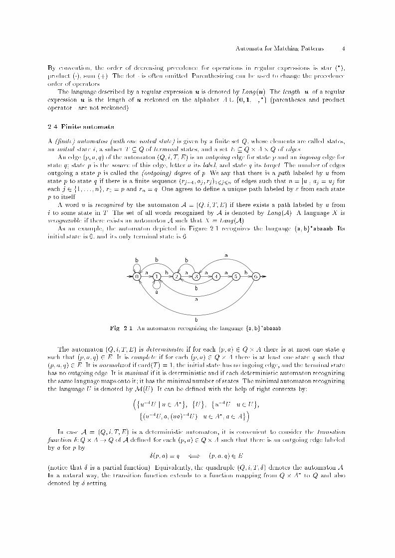
Automata for Matching Patterns 4By convention, the order of decreasing precedence for operations in regular expressions is star (�),product (�), sum (+). The dot � is often omitted. Parenthesizing can be used to change the precedenceorder of operators.The language described by a regular expression u is denoted by Lang (u). The length juj of a regularexpression u is the length of u reckoned on the alphabet A [ f0;1;+; �g (parentheses and productoperator � are not reckoned).2.4 Finite automataA (�nite) automaton (with one initial state) is given by a �nite set Q, whose elements are called states,an initial state i, a subset T � Q of terminal states, and a set E � Q�A �Q of edges.An edge (p; a; q) of the automaton (Q; i; T;E) is an outgoing edge for state p and an ingoing edge forstate q; state p is the source of this edge, letter a its label, and state q its target. The number of edgesoutgoing a state p is called the (outgoing) degree of p. We say that there is a path labeled by u fromstate p to state q if there is a �nite sequence (rj�1; aj; rj)16j6n of edges such that n = juj, aj = uj foreach j 2 f1; : : : ; ng, r0 = p and rn = q. One agrees to de�ne a unique path labeled by " from each statep to itself.A word u is recognized by the automaton A = (Q; i; T;E) if there exists a path labeled by u fromi to some state in T . The set of all words recognized by A is denoted by Lang(A). A language X isrecognizable if there exists an automaton A such that X = Lang (A).As an example, the automaton depicted in Figure 2.1 recognizes the language fa; bg�abaaab. Itsinitial state is 0, and its only terminal state is 6.0 1 2 3 4 5 6a b a a a bb ab b bab aFig. 2.1. An automaton recognizing the language fa; bg�abaaab.The automaton (Q; i; T;E) is deterministic if for each (p; a) 2 Q � A there is at most one state qsuch that (p; a; q) 2 E. It is complete if for each (p; a) 2 Q � A there is at least one state q such that(p; a; q) 2 E. It is normalized if card(T ) = 1, the initial state has no ingoing edge, and the terminal statehas no outgoing edge. It is minimal if it is deterministic and if each deterministic automaton recognizingthe same languagemaps onto it; it has the minimalnumber of states. The minimal automaton recognizingthe language U is denoted byM(U ). It can be de�ned with the help of right contexts by:��u�1U j u 2 A�; �U; �u�1U j u 2 U;�(u�1U; a; (ua)�1U ) j u 2 A�; a 2 A�In case A = (Q; i; T;E) is a deterministic automaton, it is convenient to consider the transitionfunction �:Q�A! Q of A de�ned for each (p; a) 2 Q�A such that there is an outgoing edge labeledby a for p by �(p; a) = q () (p; a; q) 2 E(notice that � is a partial function). Equivalently, the quadruple (Q; i; T; �) denotes the automaton A.In a natural way, the transition function extends to a function mapping from Q � A� to Q and alsodenoted by � setting

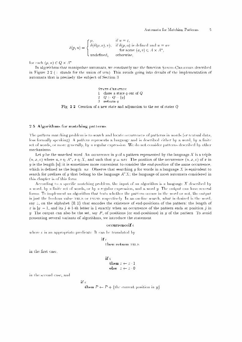
Automata for Matching Patterns 5�(p; u) = 8><>: p; if u = ",�(�(p; a); v); if �(p; a) is de�ned and u = avfor some (a; v) 2 A� A�,unde�ned; otherwise,for each (p; u) 2 Q� A�.In algorithms that manipulate automata, we constantly use the function State-Creation describedin Figure 2.2 (+ stands for the union of sets). This avoids going into details of the implementation ofautomata that is precisely the subject of Section 3.State-Creation1 chose a state q out of Q2 Q Q + fqg3 return qFig. 2.2. Creation of a new state and adjunction to the set of states Q.2.5 Algorithms for matching patternsThe pattern matching problem is to search and locate occurrences of patterns in words (or textual data,less formally speaking). A pattern represents a language and is described either by a word, by a �niteset of words, or more generally, by a regular expression. We do not consider patterns described by othermechanisms.Let y be the searched word. An occurrence in y of a pattern represented by the language X is a triple(u; x; v) where u; v 2 A�, x 2 X, and such that y = uxv. The position of the occurrence (u; x; v) of x iny is the length juj; it is sometimes more convenient to consider the end-position of the same occurrence,which is de�ned as the length juxj. Observe that searching y for words in a language X is equivalent tosearch for pre�xes of y that belong to the language A�X; the language of most automata considered inthis chapter is of this form.According to a speci�c matching problem, the input of an algorithm is a language X described bya word, by a �nite set of words, or by a regular expression, and a word y. The output can have severalforms. To implement an algorithm that tests whether the pattern occurs in the word or not, the outputis just the boolean value true or false respectively. In an on-line search, what is desired is the word,say z, on the alphabet f0; 1g that encodes the existence of end-positions of the pattern; the length ofz is jyj+ 1, and its j + 1-th letter is 1 exactly when an occurrence of the pattern ends at position j iny. The output can also be the set, say P , of positions (or end-positions) in y of the pattern. To avoidpresenting several variants of algorithms, we introduce the statementoccurrenceif ewhere e is an appropriate predicate. It can be translated byif ethen return truein the �rst case, if ethen z z � 1else z z � 0in the second case, and if ethen P P + fthe current position in yg

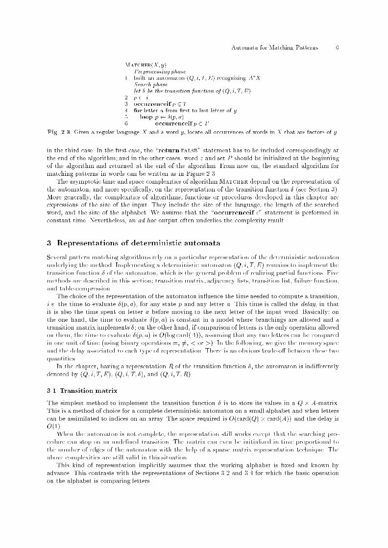
Automata for Matching Patterns 6Matcher(X;y)Preprocessing phase1 built an automaton (Q; i; T; E) recognizing A�XSearch phaselet � be the transition function of (Q; i; T; E)2 p i3 occurrenceif p 2 T4 for letter a from �rst to last letter of y5 loop p �(p; a)6 occurrenceif p 2 TFig. 2.3. Given a regular language X and a word y, locate all occurrences of words in X that are factors of y.in the third case. In the �rst case, the \return false" statement has to be included correspondingly atthe end of the algorithm; and in the other cases, word z and set P should be initialized at the beginningof the algorithm and returned at the end of the algorithm. From now on, the standard algorithm formatching patterns in words can be written as in Figure 2.3.The asymptotic time and space complexities of algorithmMatcher depend on the representation ofthe automaton, and more speci�cally, on the representation of the transition function � (see Section 3).More generally, the complexities of algorithms, functions or procedures developed in this chapter areexpressions of the size of the input. They include the size of the language, the length of the searchedword, and the size of the alphabet. We assume that the \occurrenceif e" statement is performed inconstant time. Nevertheless, an ad hoc output often underlies the complexity result.3. Representations of deterministic automataSeveral pattern matching algorithms rely on a particular representation of the deterministic automatonunderlying the method. Implementing a deterministic automaton (Q; i; T;E) remains to implement thetransition function � of the automaton, which is the general problem of realizing partial functions. Fivemethods are described in this section: transition matrix, adjacency lists, transition list, failure function,and table-compression.The choice of the representation of the automaton in uence the time needed to compute a transition,i.e. the time to evaluate �(p; a), for any state p and any letter a. This time is called the delay, in thatit is also the time spent on letter a before moving to the next letter of the input word. Basically: onthe one hand, the time to evaluate �(p; a) is constant in a model where branchings are allowed and atransition matrix implements �; on the other hand, if comparison of letters is the only operation allowedon them, the time to evaluate �(p; a) is O(log card(A)), assuming that any two letters can be comparedin one unit of time (using binary operations =, 6=, < or >). In the following, we give the memory spaceand the delay associated to each type of representation. There is an obvious trade-o� between these twoquantities.In the chapter, having a representation R of the transition function �, the automaton is indi�erentlydenoted by (Q; i; T;E), (Q; i; T; �), and (Q; i; T;R).3.1 Transition matrixThe simplest method to implement the transition function � is to store its values in a Q � A-matrix.This is a method of choice for a complete deterministic automaton on a small alphabet and when letterscan be assimilated to indices on an array. The space required is O(card(Q) � card(A)) and the delay isO(1).When the automaton is not complete, the representation still works except that the searching pro-cedure can stop on an unde�ned transition. The matrix can even be initialized in time proportional tothe number of edges of the automaton with the help of a sparse matrix representation technique. Theabove complexities are still valid in this situation.This kind of representation implicitly assumes that the working alphabet is �xed and known byadvance. This contrasts with the representations of Sections 3.2 and 3.4 for which the basic operationon the alphabet is comparing letters.

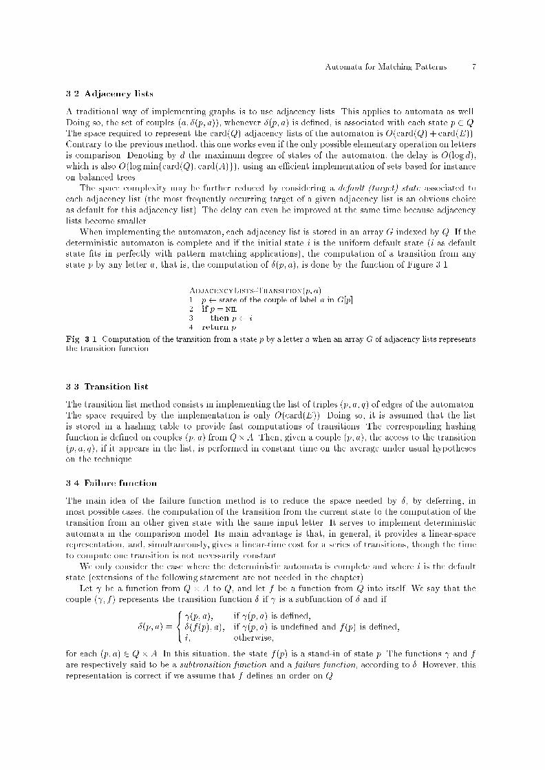
Automata for Matching Patterns 73.2 Adjacency listsA traditional way of implementing graphs is to use adjacency lists. This applies to automata as well.Doing so, the set of couples (a; �(p; a)), whenever �(p; a) is de�ned, is associated with each state p 2 Q.The space required to represent the card(Q) adjacency lists of the automaton is O(card(Q) + card(E)).Contrary to the previous method, this one works even if the only possible elementary operation on lettersis comparison. Denoting by d the maximum degree of states of the automaton, the delay is O(log d),which is also O(logminfcard(Q); card(A)g), using an e�cient implementation of sets based for instanceon balanced trees.The space complexity may be further reduced by considering a default (target) state associated toeach adjacency list (the most frequently occurring target of a given adjacency list is an obvious choiceas default for this adjacency list). The delay can even be improved at the same time because adjacencylists become smaller.When implementing the automaton, each adjacency list is stored in an array G indexed by Q. If thedeterministic automaton is complete and if the initial state i is the uniform default state (i as defaultstate �ts in perfectly with pattern matching applications), the computation of a transition from anystate p by any letter a, that is, the computation of �(p; a), is done by the function of Figure 3.1.AdjacencyLists-Transition(p; a)1 p state of the couple of label a in G[p]2 if p = nil3 then p i4 return pFig. 3.1. Computation of the transition from a state p by a letter a when an array G of adjacency lists representsthe transition function.3.3 Transition listThe transition list method consists in implementing the list of triples (p; a; q) of edges of the automaton.The space required by the implementation is only O(card(E)). Doing so, it is assumed that the listis stored in a hashing table to provide fast computations of transitions. The corresponding hashingfunction is de�ned on couples (p; a) from Q�A. Then, given a couple (p; a), the access to the transition(p; a; q), if it appears in the list, is performed in constant time on the average under usual hypotheseson the technique.3.4 Failure functionThe main idea of the failure function method is to reduce the space needed by �, by deferring, inmost possible cases, the computation of the transition from the current state to the computation of thetransition from an other given state with the same input letter. It serves to implement deterministicautomata in the comparison model. Its main advantage is that, in general, it provides a linear-spacerepresentation, and, simultaneously, gives a linear-time cost for a series of transitions, though the timeto compute one transition is not necessarily constant.We only consider the case where the deterministic automata is complete and where i is the defaultstate (extensions of the following statement are not needed in the chapter).Let be a function from Q � A to Q, and let f be a function from Q into itself. We say that thecouple ( ; f) represents the transition function � if is a subfunction of � and if�(p; a) = 8<: (p; a); if (p; a) is de�ned,�(f(p); a); if (p; a) is unde�ned and f(p) is de�ned,i; otherwise,for each (p; a) 2 Q� A. In this situation, the state f(p) is a stand-in of state p. The functions and fare respectively said to be a subtransition function and a failure function, according to �. However, thisrepresentation is correct if we assume that f de�nes an order on Q.

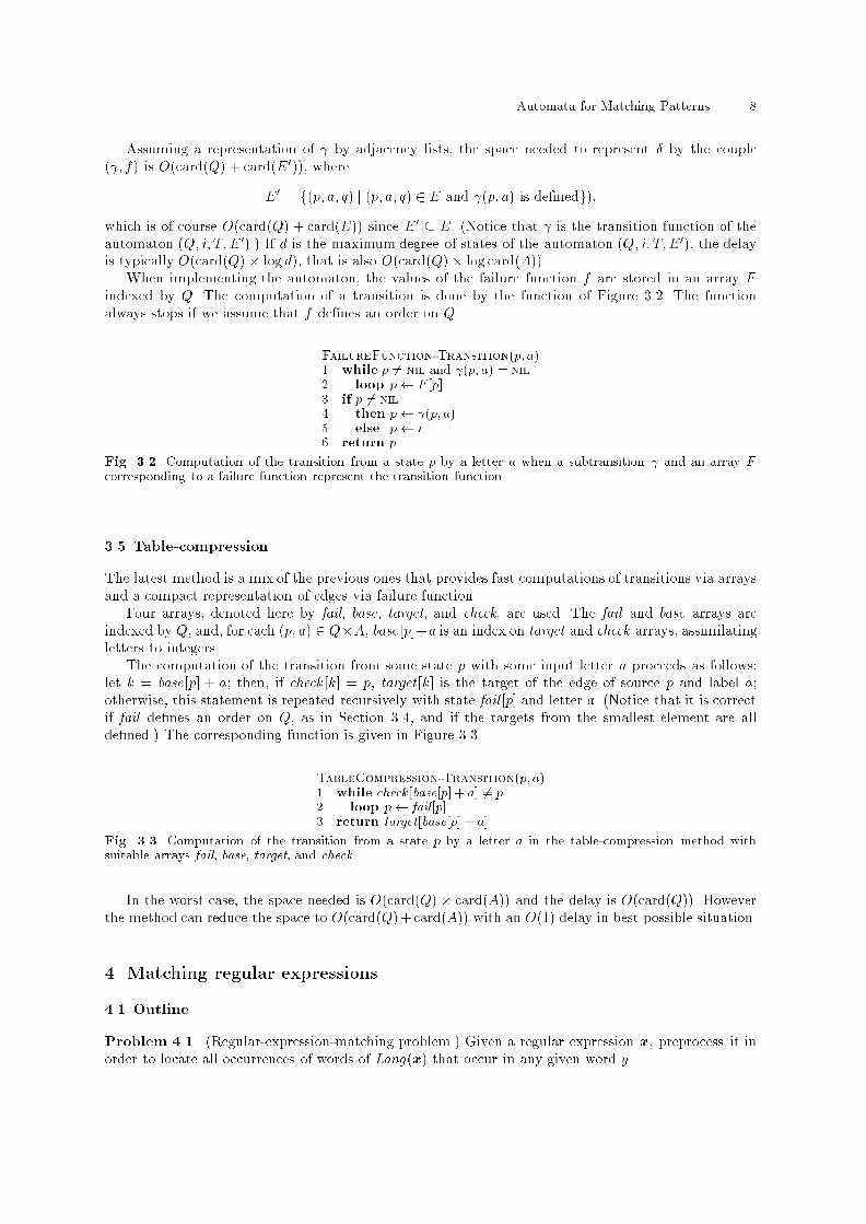
Automata for Matching Patterns 8Assuming a representation of by adjacency lists, the space needed to represent � by the couple( ; f) is O(card(Q) + card(E0)), whereE0 = f(p; a; q) j (p; a; q) 2 E and (p; a) is de�nedg);which is of course O(card(Q) + card(E)) since E0 � E. (Notice that is the transition function of theautomaton (Q; i; T;E0).) If d is the maximum degree of states of the automaton (Q; i; T;E0), the delayis typically O(card(Q) � logd), that is also O(card(Q) � log card(A)).When implementing the automaton, the values of the failure function f are stored in an array Findexed by Q. The computation of a transition is done by the function of Figure 3.2. The functionalways stops if we assume that f de�nes an order on Q.FailureFunction-Transition(p; a)1 while p 6= nil and (p; a) = nil2 loop p F [p]3 if p 6= nil4 then p (p; a)5 else p i6 return pFig. 3.2. Computation of the transition from a state p by a letter a when a subtransition and an array Fcorresponding to a failure function represent the transition function.3.5 Table-compressionThe latest method is a mix of the previous ones that provides fast computations of transitions via arraysand a compact representation of edges via failure function.Four arrays, denoted here by fail, base, target, and check, are used. The fail and base arrays areindexed by Q, and, for each (p; a) 2 Q�A, base [p]+a is an index on target and check arrays, assimilatingletters to integers.The computation of the transition from some state p with some input letter a proceeds as follows:let k = base[p] + a; then, if check [k] = p, target[k] is the target of the edge of source p and label a;otherwise, this statement is repeated recursively with state fail [p] and letter a. (Notice that it is correctif fail de�nes an order on Q, as in Section 3.4, and if the targets from the smallest element are allde�ned.) The corresponding function is given in Figure 3.3.TableCompression-Transition(p; a)1 while check[base[p] + a] 6= p2 loop p fail[p]3 return target[base[p] + a]Fig. 3.3. Computation of the transition from a state p by a letter a in the table-compression method withsuitable arrays fail, base, target, and check.In the worst case, the space needed is O(card(Q) � card(A)) and the delay is O(card(Q)). Howeverthe method can reduce the space to O(card(Q)+card(A)) with an O(1) delay in best possible situation.4. Matching regular expressions4.1 OutlineProblem 4.1. (Regular-expression-matching problem.) Given a regular expression x, preprocess it inorder to locate all occurrences of words of Lang(x) that occur in any given word y.

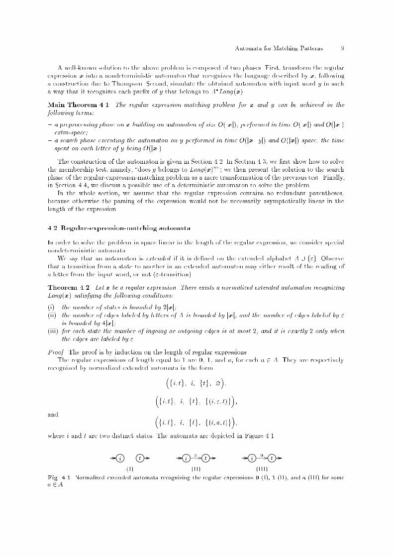
Automata for Matching Patterns 9A well-known solution to the above problem is composed of two phases. First, transform the regularexpression x into a nondeterministic automaton that recognizes the language described by x, followinga construction due to Thompson. Second, simulate the obtained automaton with input word y in sucha way that it recognizes each pre�x of y that belongs to A�Lang (x).Main Theorem 4.1. The regular expression-matching problem for x and y can be achieved in thefollowing terms:{ a preprocessing phase on x building an automaton of size O(jxj), performed in time O(jxj) and O(jxj)extra-space;{ a search phase executing the automaton on y performed in time O(jxj jyj) and O(jxj) space, the timespent on each letter of y being O(jxj).The construction of the automaton is given in Section 4.2. In Section 4.3, we �rst show how to solvethe membership test, namely, \does y belongs to Lang(x)?"; we then present the solution to the searchphase of the regular-expression-matching problem as a mere transformation of the previous test. Finally,in Section 4.4, we discuss a possible use of a deterministic automaton to solve the problem.In the whole section, we assume that the regular expression contains no redundant parentheses,because otherwise the parsing of the expression would not be necessarily asymptotically linear in thelength of the expression.4.2 Regular-expression-matching automataIn order to solve the problem in space linear in the length of the regular expression, we consider specialnondeterministic automata.We say that an automaton is extended if it is de�ned on the extended alphabet A [ f"g. Observethat a transition from a state to another in an extended automaton may either result of the reading ofa letter from the input word, or not ("-transition).Theorem 4.2. Let x be a regular expression. There exists a normalized extended automaton recognizingLang(x) satisfying the following conditions:(i) the number of states is bounded by 2jxj;(ii) the number of edges labeled by letters of A is bounded by jxj, and the number of edges labeled by "is bounded by 4jxj;(iii) for each state the number of ingoing or outgoing edges is at most 2, and it is exactly 2 only whenthe edges are labeled by ".Proof. The proof is by induction on the length of regular expressions.The regular expressions of length equal to 1 are 0, 1, and a, for each a 2 A. They are respectivelyrecognized by normalized extended automata in the form��i; t; i; �t; ?�;��i; t; i; �t; �(i; "; t)�;and ��i; t; i; �t; �(i; a; t)�;where i and t are two distinct states. The automata are depicted in Figure 4.1.i t i t" i ta(I) (II) (III)Fig. 4.1. Normalized extended automata recognizing the regular expressions 0 (I), 1 (II), and a (III) for somea 2 A.

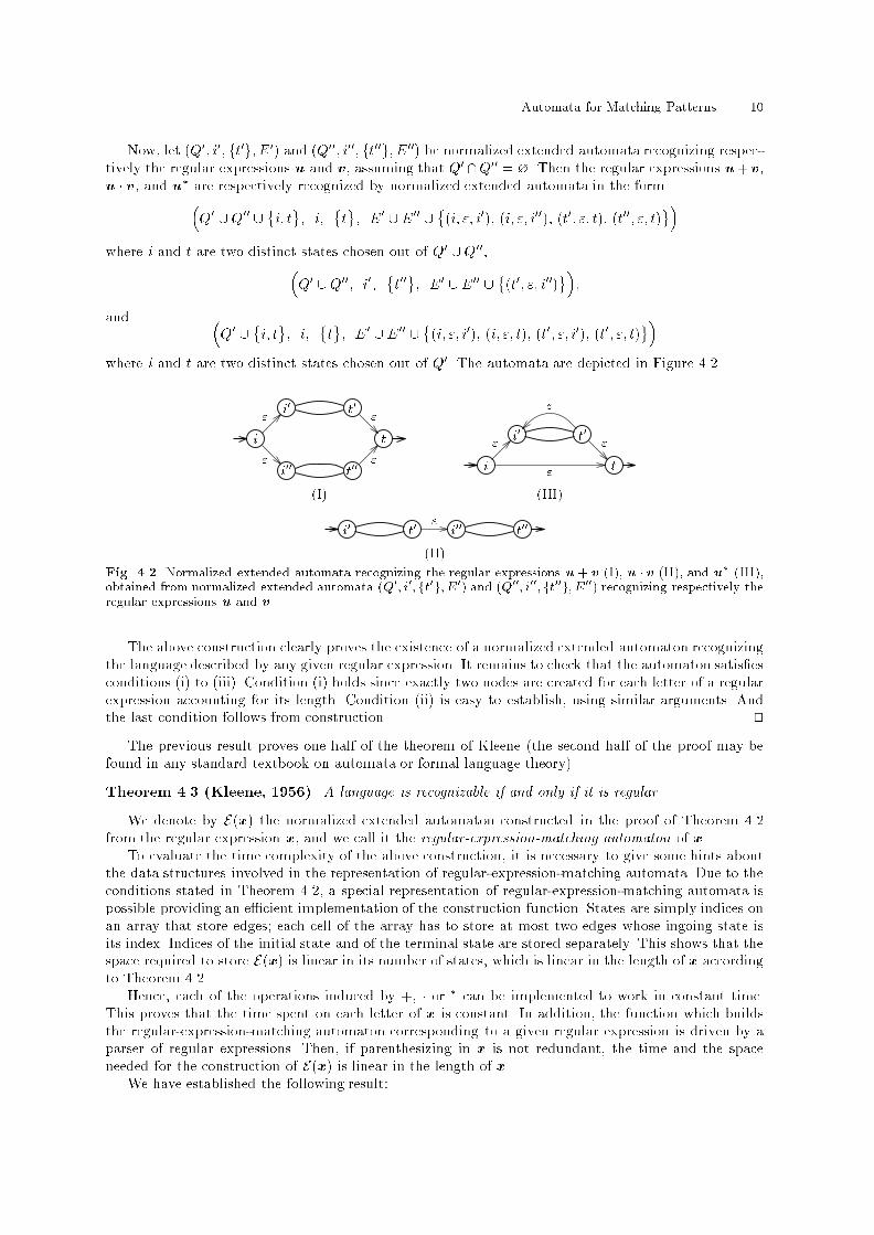
Automata for Matching Patterns 10Now, let (Q0; i0; ft0g; E0) and (Q00; i00; ft00g; E00) be normalized extended automata recognizing respec-tively the regular expressions u and v, assuming that Q0\Q00 = ?. Then the regular expressions u+v,u � v, and u� are respectively recognized by normalized extended automata in the form�Q0 [Q00 [ �i; t; i; �t; E0 [E00 [ �(i; "; i0); (i; "; i00); (t0; "; t); (t00; "; t)�where i and t are two distinct states chosen out of Q0 [Q00,�Q0 [Q00; i0; �t00; E0 [E00 [ �(t0; "; i00)�;and �Q0 [ �i; t; i; �t; E0 [E00 [ �(i; "; i0); (i; "; t); (t0; "; i0); (t0; "; t)�where i and t are two distinct states chosen out of Q0. The automata are depicted in Figure 4.2.i i0 t0i00 t00 t"" "" i i0 t0 t" """(I) (III)i0 t0 i00 t00"(II)Fig. 4.2. Normalized extended automata recognizing the regular expressions u+ v (I), u � v (II), and u� (III),obtained from normalized extended automata (Q0; i0; ft0g; E0) and (Q00; i00; ft00g; E00) recognizing respectively theregular expressions u and v.The above construction clearly proves the existence of a normalized extended automaton recognizingthe language described by any given regular expression. It remains to check that the automaton satis�esconditions (i) to (iii). Condition (i) holds since exactly two nodes are created for each letter of a regularexpression accounting for its length. Condition (ii) is easy to establish, using similar arguments. Andthe last condition follows from construction. utThe previous result proves one half of the theorem of Kleene (the second half of the proof may befound in any standard textbook on automata or formal language theory).Theorem 4.3 (Kleene, 1956). A language is recognizable if and only if it is regular.We denote by E(x) the normalized extended automaton constructed in the proof of Theorem 4.2from the regular expression x, and we call it the regular-expression-matching automaton of x.To evaluate the time complexity of the above construction, it is necessary to give some hints aboutthe data structures involved in the representation of regular-expression-matching automata. Due to theconditions stated in Theorem 4.2, a special representation of regular-expression-matching automata ispossible providing an e�cient implementation of the construction function. States are simply indices onan array that store edges; each cell of the array has to store at most two edges whose ingoing state isits index. Indices of the initial state and of the terminal state are stored separately. This shows that thespace required to store E(x) is linear in its number of states, which is linear in the length of x accordingto Theorem 4.2.Hence, each of the operations induced by +, � or � can be implemented to work in constant time.This proves that the time spent on each letter of x is constant. In addition, the function which buildsthe regular-expression-matching automaton corresponding to a given regular expression is driven by aparser of regular expressions. Then, if parenthesizing in x is not redundant, the time and the spaceneeded for the construction of E(x) is linear in the length of x.We have established the following result:

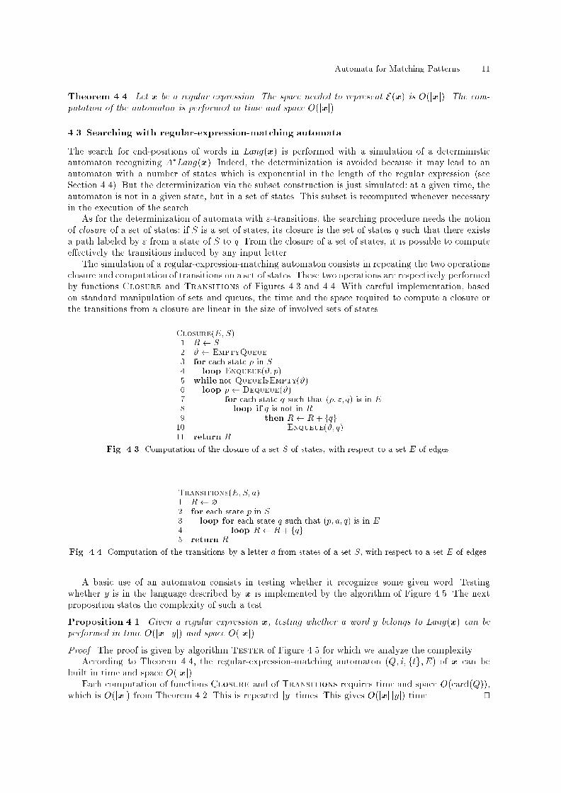
Automata for Matching Patterns 11Theorem 4.4. Let x be a regular expression. The space needed to represent E(x) is O(jxj). The com-putation of the automaton is performed in time and space O(jxj).4.3 Searching with regular-expression-matching automataThe search for end-positions of words in Lang(x) is performed with a simulation of a deterministicautomaton recognizing A�Lang(x). Indeed, the determinization is avoided because it may lead to anautomaton with a number of states which is exponential in the length of the regular expression (seeSection 4.4). But the determinization via the subset construction is just simulated: at a given time, theautomaton is not in a given state, but in a set of states. This subset is recomputed whenever necessaryin the execution of the search.As for the determinization of automata with "-transitions, the searching procedure needs the notionof closure of a set of states: if S is a set of states, its closure is the set of states q such that there existsa path labeled by " from a state of S to q. From the closure of a set of states, it is possible to computee�ectively the transitions induced by any input letter.The simulation of a regular-expression-matching automaton consists in repeating the two operationsclosure and computation of transitions on a set of states. These two operations are respectively performedby functions Closure and Transitions of Figures 4.3 and 4.4. With careful implementation, basedon standard manipulation of sets and queues, the time and the space required to compute a closure orthe transitions from a closure are linear in the size of involved sets of states.Closure(E; S)1 R S2 # EmptyQueue3 for each state p in S4 loop Enqueue(#; p)5 while not QueueIsEmpty(#)6 loop p Dequeue(#)7 for each state q such that (p; "; q) is in E8 loop if q is not in R9 then R R+ fqg10 Enqueue(#;q)11 return RFig. 4.3. Computation of the closure of a set S of states, with respect to a set E of edges.Transitions(E;S; a)1 R ?2 for each state p in S3 loop for each state q such that (p; a; q) is in E4 loop R R+ fqg5 return RFig. 4.4. Computation of the transitions by a letter a from states of a set S, with respect to a set E of edges.A basic use of an automaton consists in testing whether it recognizes some given word. Testingwhether y is in the language described by x is implemented by the algorithm of Figure 4.5. The nextproposition states the complexity of such a test.Proposition 4.1. Given a regular expression x, testing whether a word y belongs to Lang(x) can beperformed in time O(jxj jyj) and space O(jxj).Proof. The proof is given by algorithm Tester of Figure 4.5 for which we analyze the complexity.According to Theorem 4.4, the regular-expression-matching automaton (Q; i; ftg; E) of x can bebuilt in time and space O(jxj).Each computation of functions Closure and of Transitions requires time and space O(card(Q)),which is O(jxj) from Theorem 4.2. This is repeated jyj times. This gives O(jxj jyj) time. ut

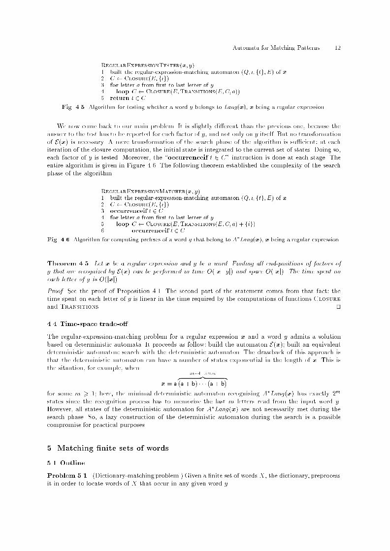
Automata for Matching Patterns 12RegularExpressionTester(x; y)1 built the regular-expression-matching automaton (Q; i; ftg; E) of x2 C Closure(E; fig)3 for letter a from �rst to last letter of y4 loop C Closure(E;Transitions(E;C; a))5 return t 2 CFig. 4.5. Algorithm for testing whether a word y belongs to Lang(x), x being a regular expression.We now come back to our main problem. It is slightly di�erent than the previous one, because theanswer to the test has to be reported for each factor of y, and not only on y itself. But no transformationof E(x) is necessary. A mere transformation of the search phase of the algorithm is su�cient: at eachiteration of the closure computation, the initial state is integrated to the current set of states. Doing so,each factor of y is tested. Moreover, the \occurrenceif t 2 C" instruction is done at each stage. Theentire algorithm is given in Figure 4.6. The following theorem established the complexity of the searchphase of the algorithm.RegularExpressionMatcher(x; y)1 built the regular-expression-matching automaton (Q; i; ftg; E) of x2 C Closure(E; fig)3 occurrenceif t 2 C4 for letter a from �rst to last letter of y5 loop C Closure(E;Transitions(E;C; a) + fig)6 occurrenceif t 2 CFig. 4.6. Algorithm for computing pre�xes of a word y that belong to A�Lang(x), x being a regular expression.Theorem 4.5. Let x be a regular expression and y be a word. Finding all end-positions of factors ofy that are recognized by E(x) can be performed in time O(jxj jyj) and space O(jxj). The time spent oneach letter of y is O(jxj).Proof. See the proof of Proposition 4.1. The second part of the statement comes from that fact: thetime spent on each letter of y is linear in the time required by the computations of functions Closureand Transitions. ut4.4 Time-space trade-o�The regular-expression-matching problem for a regular expression x and a word y admits a solutionbased on deterministic automata. It proceeds as follow: build the automaton E(x); built an equivalentdeterministic automaton; search with the deterministic automaton. The drawback of this approach isthat the deterministic automaton can have a number of states exponential in the length of x. This isthe situation, for example, when x = a m�1 timesz }| {(a + b) � � � (a+ b)for some m > 1; here, the minimal deterministic automaton recognizing A�Lang(x) has exactly 2mstates since the recognition process has to memorize the last m letters read from the input word y.However, all states of the deterministic automaton for A�Lang(x) are not necessarily met during thesearch phase. So, a lazy construction of the deterministic automaton during the search is a possiblecompromise for practical purposes.5. Matching �nite sets of words5.1 OutlineProblem 5.1. (Dictionary-matching problem.) Given a �nite set of words X, the dictionary, preprocessit in order to locate words of X that occur in any given word y.

Automata for Matching Patterns 13The classical solution to this problem is due to Aho and Corasick. It essentially consists in a linear-space implementation of a complete deterministic automaton recognizing the language A�X. The im-plementation uses both adjacency lists and an appropriate failure function.Main Theorem 5.1 (Aho and Corasick, 1975). The dictionary-matching problem for X and y canbe achieved in the following terms:{ a preprocessing phase on X building an implementation of size O(jXj) of an automaton recognizingA�X, performed in time O(jXj � log card(A)) and O(card(X)) extra-space;{ a search phase executing the automaton on y performed in time O(jyj � log card(A)) and constantextra-space, the delay being O(jXj � log card(A)).If we allow more extra-space, the asymptotic time complexities can be reduced. This is achieved, forinstance, by using techniques of Section 3 for representing deterministic automata with a sparse matrix,and assuming that O(jXj � card(A)) space is available. The time complexities of the preprocessing andsearch phases are respectively reduced to O(jXj) and O(jyj), and the delay to O(jXj). Nevertheless,notice that the times complexities given in the above theorem are still linear in jXj or jyj if we consider�xed alphabets.The method behind Theorem 5.1 is based on a speci�c automaton recognizing A�X: its states arethe pre�xes of words in X (their number is �nite as X is). The automaton is not minimal in the generalcase. It is presented in Section 5.2, and its implementation with a failure function is given in Section 5.3.Section 5.4 is devoted to the search for X with the automaton.5.2 Dictionary-matching automataWe give a complete deterministic automaton that recognizes A�X. In order to formalize this automaton,we introduce for each language U the mapping hU :A� ! Pref (U ) de�ned for each word v byhU (v) = the longest su�x of v that belongs to Pref (U ):(In the whole Section 5, U refers to an ordinary language, and X refers to a �nite language.)Proposition 5.1. Let X be a �nite language. Then the automaton�Pref (X); "; Pref (X) \A�X; �(p; a; hX(pa)) j p 2 Pref (X); a 2 A�recognizes the language A�X. This automaton is deterministic and complete.In the following, we denote by D(X) the automaton of Proposition 5.1 applied to X, and we call itthe dictionary-matching automaton of X.The proof of Proposition 5.1 relies on the following result.Lemma 5.1. Let U � A�. Then(i) v 2 A�U i� hU (v) 2 A�U , for each v 2 A�.Furthermore, hU satis�es the relations:(ii) hU(") = ";(iii) hU(va) = hU(hU (v)a), for each (v; a) 2 A� �A.Proof. If v 2 A�U , then v is in the form wu where w 2 A� and u 2 U ; by de�nition of hU , u is necessarilya su�x of hU (v); therefore hU (v) 2 A�U . Conversely, if hU (v) 2 A�U , we have also v 2 A�U , becausehU (v) is a su�x of v. Which proves (i).Property (ii) clearly holds.It remains to prove (iii). Both words hU (va) and hU(v)a are su�xes of va, and therefore one of themis a su�x of the other. Then we distinguish two cases according to which word is a su�x of the other.First case: hU (v)a is a proper su�x of hU (va) (hence hU (va) 6= "). Consider the word w de�ned byw = hU (va)a�1. Thus we have: hU (v) is a proper su�x of w, w is a su�x of v, and since hU (va) 2

Automata for Matching Patterns 14Pref (U ), w 2 Pref (U ). Whence w is a su�x of v that belongs to Pref (U ), but strictly longest thanhU (v). This contradicts the maximality of jhU(v)j. So this case is impossible.Second case: hU (va) is a su�x of hU (v)a. Then, hU(va) is a su�x of hU (hU(v)a). Now, since hU (v)ais a su�x of va, hU (hU(v)a) is a su�x of hU (va). Both properties implies hU(va) = hU(hU (v)a), andthe expected result follows. utProof of Proposition 5.1. Let v 2 A�. It follows from properties (ii) and (iii) of Lemma 5.1 that�hX(v1v2 � � �vj�1); vi; hX(v1v2 � � �vj)�16j6jvjis a path labeled by v from the initial state " to the state hX (v).If v 2 A�X, we get hX (v) 2 A�X from (i) of Lemma 5.1; which shows that hX (v) is a terminal state,and �nally that v is recognized by the automaton.Conversely, if v is recognized by the automaton,we have hX(v) 2 A�X by de�nition of the automaton.This implies that v 2 A�X from (i) of Lemma 5.1 again. utWe show how to implement the automaton D(X) in the next section.5.3 Linear dictionary-matching automataThe automaton D(X) is implemented with a failure function. The aim is to get a representation thatdoes not depend on the size of the alphabet.For each language U , let fU :Pref (U )! Pref (U ) be the function de�ned for each nonempty word uin Pref (U ) by fU (u) = the longest proper su�x of u that belongs to Pref (U ):Lemma 5.2. Let U � A�. For each (u; a) 2 Pref (U ) �A, we have:hU (ua) = 8<:ua; if ua 2 Pref (U ),hU (fU (u)a); if u 6= " and ua 62 Pref (U ),"; otherwise.Proof. The identity clearly holds when ua 2 Pref (U ) or when ua 62 Pref (U ) but u = ".It remains to examine the case where ua 62 Pref (U ) and u 6= ". Here, fU (u)a is a proper su�x of ua.What is more, hU(fU (u)a) is the longest su�x of ua that belongs to Pref (U ). Indeed, if we assume theexistence of a su�x v of ua satisfying v 2 Pref (U ) and jvj > jfU(v)aj, we get that va�1 is a proper su�xof u belonging to Pref (U ); then va�1 = fU (u) because of the maximality of jfU (u)j. Which achieves theproof. utWe introduce for each language U the function U :Pref (U ) � A ! Pref (U ) associating with each(u; a) 2 Pref (U ) � A such that ua 2 Pref (U ) the word ua. Thus, with conventions of Section 3.4, wehave:Proposition 5.2. For each �nite language X, the couple ( X ; fX) represents the transition functionof D(X); function X is a subtransition function and function fx a failure function, according to thetransition function of D(X).Proof. Follows from Lemma 5.2. utNow, let us observe that function X is exactly the transition function of the deterministic automaton�Pref (X); "; X; �(p; a; pa) j p 2 Pref (X); a 2 A; pa 2 Pref (X)�:This automaton recognizes the language X, and is classically called the trie of X, as a reference to\information retrieval". It is built by function Trie of Figure 5.1.Proposition 5.3. Function Trie applied to any �nite language X builds the trie of X. If the edges ofthe automaton are implemented via adjacency lists, the size of the trie is O(jXj), and the constructionis performed in time O(jXj � log d) within constant extra-space, d being the maximum degree of states.

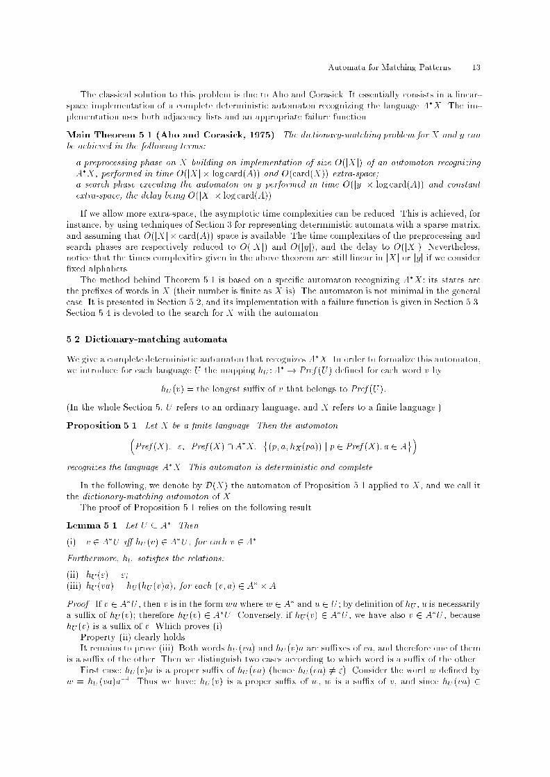
Automata for Matching Patterns 15Trie(X)let � be the transition function of (Q; i; T;E)1 (Q;T;E) (?;?;?)2 i State-Creation3 for word x from �rst to last word of X4 loop t i5 for letter a from �rst to last letter of x6 loop q �(t; a)7 if q = nil8 then q State-Creation9 E E + f(t; a; q)g10 t q11 T T + ftg12 return (Q; i; T; E)Fig. 5.1. Construction of the trie of a �nite set of words X.0 1 23 4 5 67a bb a b bbFig. 5.2. The trie of fab; babb; bbg.When X = fab; babb; bbg, the trie of X is as depicted in Figure 5.2. This example shall be consideredtwice in the following.To achieve the goal of implementing D(X) in linear size, we use Proposition 5.2. Then, it remainsto give methods for computing fX and for marking the set of terminal states. This can be done by abreadth �rst search on the graph underlying the trie starting at the initial state, as shown by the twofollowing lemmas.Lemma 5.3. Let U � A�. For each (u; a) 2 Pref (U ) �A, we have:fU (ua) = �hU (fU (u)a); if u 6= ","; otherwise.Proof. Similar to the proof of Lemma 5.2. utLemma 5.4. Let U � A�. For each u 2 Pref (U ), we have:u 2 A�U () (u 2 U ) or (u 6= " and fU (u) 2 A�U ):Proof. It is clearly su�cient to prove thatu 2 (A�U )nU =) fU (u) 2 A�U:So, let u 2 (A�U )nU . The word u is in the form vw where v 2 A� and w is a proper su�x of ubelonging to U . Then, by de�nition of fU , w is a su�x of fU (u). Therefore fU (u) 2 A�U . Which endsthe proof. utThe complete function constructing the representation of D(X) with the subtransition X and thefailure function fX is given in Figure 5.3. Let us recall that the transition function � of D(X) is assumedto be computed by function FailureFunction-Transition of Section 3.4. The next theorem statesthe correctness of the construction and its time and space complexities. We call this representationof D(X) the linear dictionary-matching automaton of X. The term \linear" (in jXj is understood) issuitable if we work with a �xed alphabet, since degrees are upper-bounded by card(A).

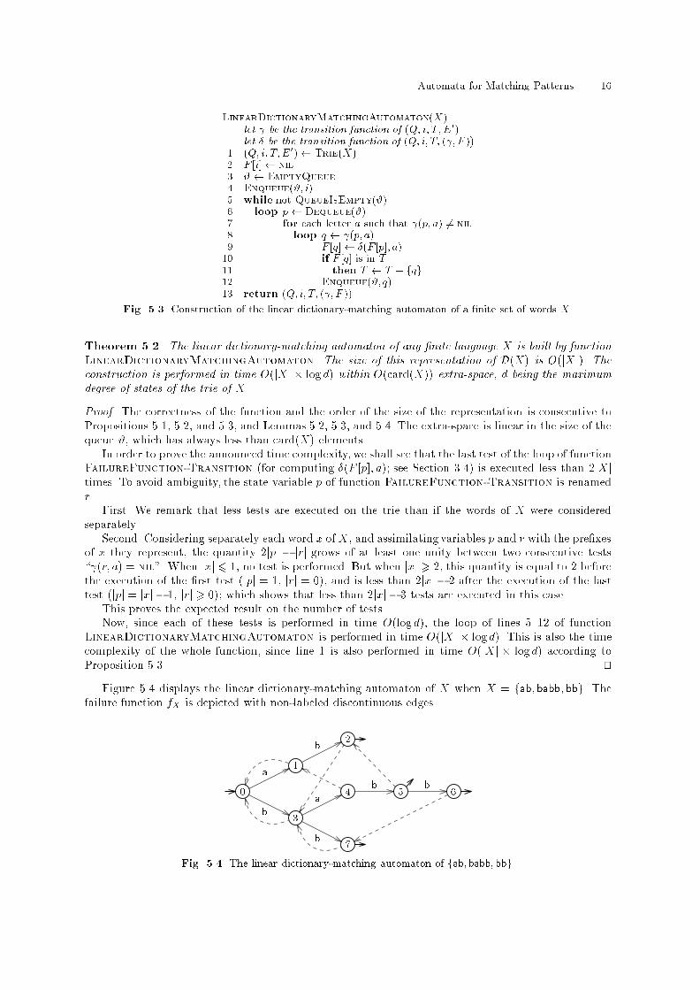
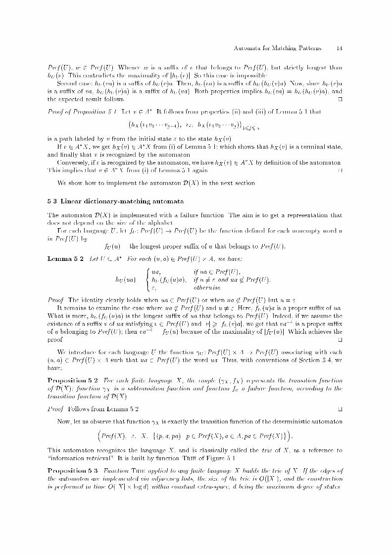
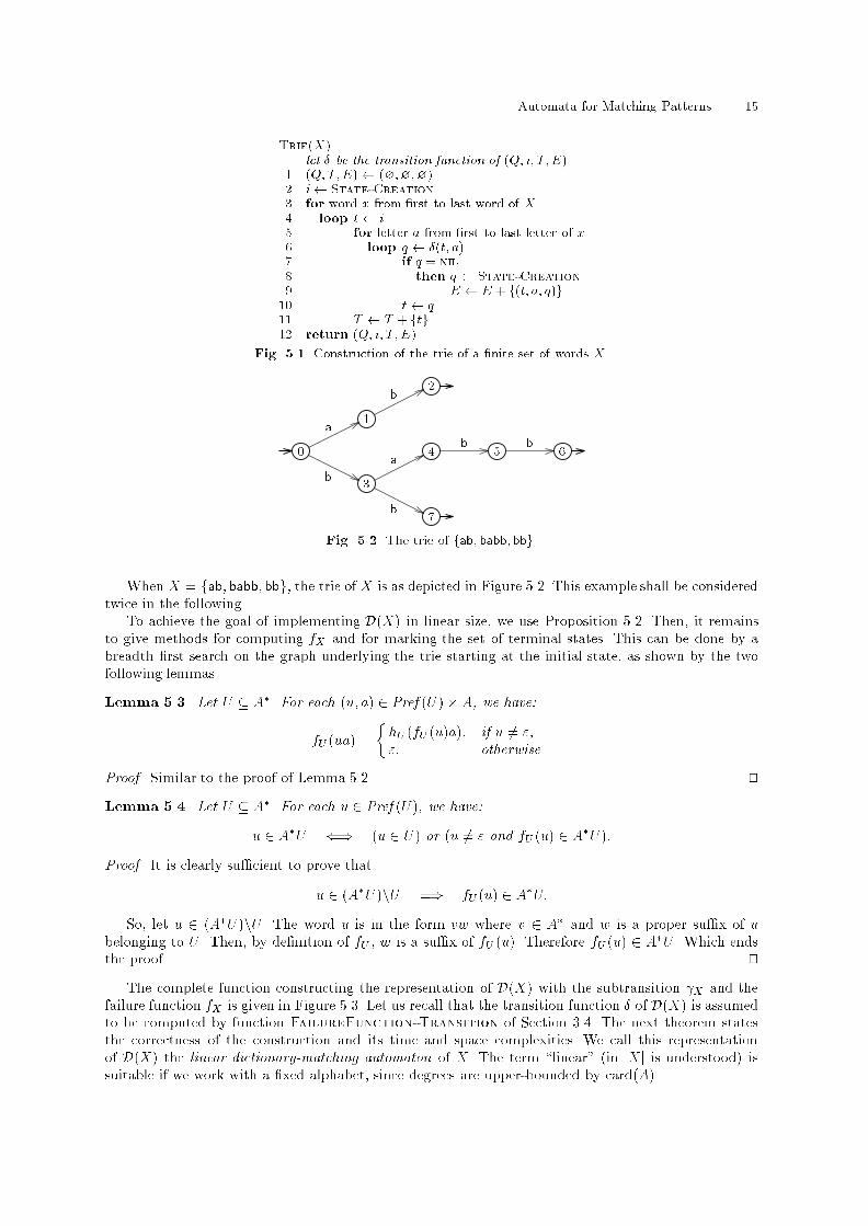
Automata for Matching Patterns 16LinearDictionaryMatchingAutomaton(X)let be the transition function of (Q; i; T; E0)let � be the transition function of (Q; i; T; ( ;F ))1 (Q; i; T;E0) Trie(X)2 F [i] nil3 # EmptyQueue4 Enqueue(#; i)5 while not QueueIsEmpty(#)6 loop p Dequeue(#)7 for each letter a such that (p; a) 6= nil8 loop q (p; a)9 F [q] �(F [p]; a)10 if F [q] is in T11 then T T + fqg12 Enqueue(#;q)13 return (Q; i; T; ( ;F ))Fig. 5.3. Construction of the linear dictionary-matching automaton of a �nite set of words X.Theorem 5.2. The linear dictionary-matching automaton of any �nite language X is built by functionLinearDictionaryMatchingAutomaton. The size of this representation of D(X) is O(jXj). Theconstruction is performed in time O(jXj � log d) within O(card(X)) extra-space, d being the maximumdegree of states of the trie of X.Proof. The correctness of the function and the order of the size of the representation is consecutive toPropositions 5.1, 5.2, and 5.3, and Lemmas 5.2, 5.3, and 5.4. The extra-space is linear in the size of thequeue #, which has always less than card(X) elements.In order to prove the announced time complexity, we shall see that the last test of the loop of functionFailureFunction-Transition (for computing �(F [p]; a); see Section 3.4) is executed less than 2jXjtimes. To avoid ambiguity, the state variable p of function FailureFunction-Transition is renamedr. First. We remark that less tests are executed on the trie than if the words of X were consideredseparately.Second. Considering separately each word x ofX, and assimilating variables p and r with the pre�xesof x they represent, the quantity 2jpj � jrj grows of at least one unity between two consecutive tests\ (r; a) = nil". When jxj 6 1, no test is performed. But when jxj > 2, this quantity is equal to 2 beforethe execution of the �rst test (jpj = 1, jrj = 0), and is less than 2jxj � 2 after the execution of the lasttest (jpj = jxj � 1, jrj > 0); which shows that less than 2jxj � 3 tests are executed in this case.This proves the expected result on the number of tests.Now, since each of these tests is performed in time O(logd), the loop of lines 5{12 of functionLinearDictionaryMatchingAutomaton is performed in time O(jXj � logd). This is also the timecomplexity of the whole function, since line 1 is also performed in time O(jXj � logd) according toProposition 5.3. utFigure 5.4 displays the linear dictionary-matching automaton of X when X = fab; babb; bbg. Thefailure function fX is depicted with non-labeled discontinuous edges.0 1 23 4 5 67a bb a b bbFig. 5.4. The linear dictionary-matching automaton of fab; babb; bbg.

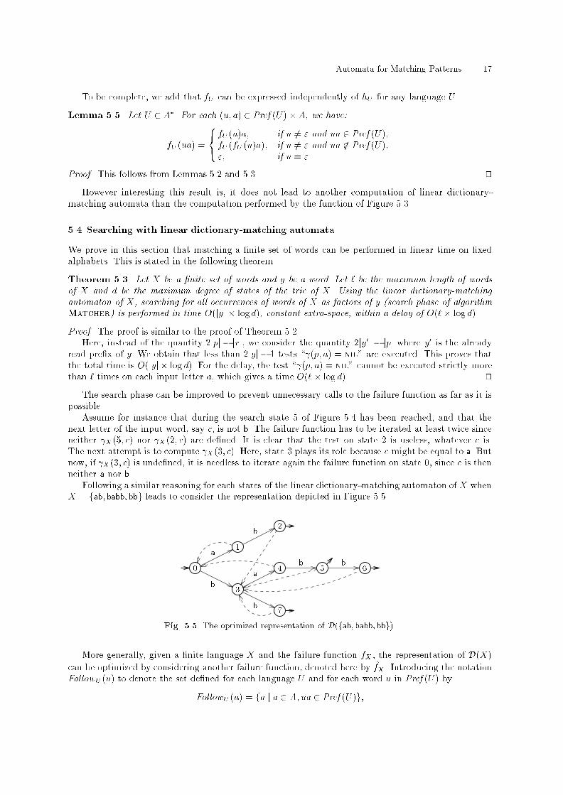
Automata for Matching Patterns 17To be complete, we add that fU can be expressed independently of hU for any language U .Lemma 5.5. Let U 2 A�. For each (u; a) 2 Pref (U )�A, we have:fU (ua) = 8<: fU (u)a; if u 6= " and ua 2 Pref (U ),fU (fU (u)a); if u 6= " and ua 62 Pref (U ),"; if u = ".Proof. This follows from Lemmas 5.2 and 5.3. utHowever interesting this result is, it does not lead to another computation of linear dictionary-matching automata than the computation performed by the function of Figure 5.3.5.4 Searching with linear dictionary-matching automataWe prove in this section that matching a �nite set of words can be performed in linear time on �xedalphabets. This is stated in the following theorem.Theorem 5.3. Let X be a �nite set of words and y be a word. Let ` be the maximum length of wordsof X and d be the maximum degree of states of the trie of X. Using the linear dictionary-matchingautomaton of X, searching for all occurrences of words of X as factors of y (search phase of algorithmMatcher) is performed in time O(jyj � logd), constant extra-space, within a delay of O(`� log d).Proof. The proof is similar to the proof of Theorem 5.2.Here, instead of the quantity 2jpj � jrj, we consider the quantity 2jy0j � jpj where y0 is the alreadyread pre�x of y. We obtain that less than 2jyj � 1 tests \ (p; a) = nil" are executed. This proves thatthe total time is O(jyj � log d). For the delay, the test \ (p; a) = nil" cannot be executed strictly morethan ` times on each input letter a, which gives a time O(` � log d). utThe search phase can be improved to prevent unnecessary calls to the failure function as far as it ispossible.Assume for instance that during the search state 5 of Figure 5.4 has been reached, and that thenext letter of the input word, say c, is not b. The failure function has to be iterated at least twice sinceneither X (5; c) nor X (2; c) are de�ned. It is clear that the test on state 2 is useless, whatever c is.The next attempt is to compute X (3; c). Here, state 3 plays its role because c might be equal to a. Butnow, if X (3; c) is unde�ned, it is needless to iterate again the failure function on state 0, since c is thenneither a nor b.Following a similar reasoning for each states of the linear dictionary-matching automaton of X whenX = fab; babb; bbg leads to consider the representation depicted in Figure 5.5.0 1 23 4 5 67a bb a b bbFig. 5.5. The optimized representation of D(fab; babb; bbg).More generally, given a �nite language X and the failure function fX , the representation of D(X)can be optimized by considering another failure function, denoted here by f̂X . Introducing the notationFollowU (u) to denote the set de�ned for each language U and for each word u in Pref (U ) byFollowU (u) = fa j a 2 A; ua 2 Pref (U )g;

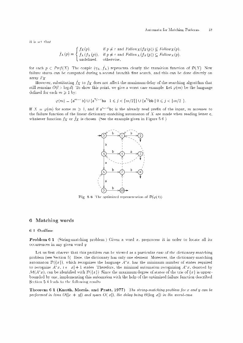
Automata for Matching Patterns 18it is set that f̂X (p) = 8<: fX (p); if p 6= " and FollowX(fX (p)) * FollowX(p),f̂X (fX (p)); if p 6= " and FollowX(fX (p)) � FollowX(p),unde�ned; otherwise,for each p 2 Pref (X). The couple ( X ; f̂X) represents clearly the transition function of D(X). Newfailure states can be computed during a second breadth �rst search, and this can be done directly onarray FX .However, substituting f̂X to fX does not a�ect the maximum delay of the searching algorithm thatstill remains O(l � log d). To show this point, we give a worst case example. Let '(m) be the languagede�ned for each m > 1 by:'(m) = fam�1bg [ fa2j�1ba j 1 6 j < dm=2eg [ fa2jbb j 0 6 j < bm=2cg:If X = '(m) for some m > 1, and if am�1bc is the already read pre�x of the input, m accesses tothe failure function of the linear dictionary-matching automaton of X are made when reading letter c,whatever function fX or f̂X is chosen. (See the example given in Figure 5.6.)0 1 23 4 56 7 89 10b ba b aa b ba bFig. 5.6. The optimized representation of D('(4)).6. Matching words6.1 OutlineProblem 6.1. (String-matching problem.) Given a word x, preprocess it in order to locate all itsoccurrences in any given word y.Let us �rst observe that this problem can be viewed as a particular case of the dictionary-matchingproblem (see Section 5). Here, the dictionary has only one element. Moreover, the dictionary-matchingautomaton D(fxg), which recognizes the language A�x, has the minimum number of states requiredto recognize A�x, i.e. jxj + 1 states. Therefore, the minimal automaton recognizing A�x, denoted byM(A�x), can be identi�ed with D(fxg). Since the maximumdegree of states of the trie of fxg is upper-bounded by one, implementing this automaton with the help of the optimized failure function describedSection 5.4 leads to the following results.Theorem 6.1 (Knuth, Morris, and Pratt, 1977). The string-matching problem for x and y can beperformed in time O(jxj+ jyj) and space O(jxj), the delay being �(log jxj) in the worst-case.

Automata for Matching Patterns 19We just have to hark back to the order of the delay for the algorithm of Knuth, Morris and Pratt. Itis proved that the number of times the transition function of the trie of fxg is performed on any inputletter cannot exceed blog�(jxj + 1)c where � = �1 + p5�=2 is the golden ratio. This upper bound isa consequence of a combinatorial property of words due to Fine and Wilf (known as the \periodicitylemma"). But it is closed to the worst-case bound, obtained when x is a pre�x of the in�nite Fibonacciword (see Chapter \Combinatorics of words").However, as we shall see, implementing M(A�x) with adjacency lists solves the string-matchingproblem with the additional feature of having a real-time search phase on �xed alphabets, i.e. with adelay bounded by a constant.Main Theorem 6.2. The string-matching problem for x and y can be achieved in the following terms:{ a preprocessing phase on x building an implementation of M(A�x) of size O(jxj), performed in timeO(jxj) and constant extra-space;{ a search phase executing the automaton on y performed in time O(jyj) and constant extra-space, thedelay being O(logminf1 + blog2 jxjc; card(A)g).Underlying the above result are indeed optimal bounds on the complexity of string-matching algo-rithms for which the search phase is on-line with a one-letter bu�er. Relaxing the on-line condition leadsto another theorem stated below. But its proof is based on combinatorial properties of words unrelatedto automata and not considered in this chapter.Theorem 6.3 (Galil and Seiferas, 1983). The string-matching problem for x and y previously storedin memory can be performed in time O(jxj+ jyj) and constant extra-space.In Section 6.2, we describe an on-line construction ofM(A�x). The linear implementation via adja-cency lists is discussed in Section 6.3. We establish in Section 6.4 properties of M(A�x) that are usedin Section 6.5 to prove the asymptotic bounds of the search phase claimed in Theorem 6.2.6.2 String-matching automataWe give a method to build the automatonM(A�x). The feature of this method is that it is based on anon-line construction and that it does not use the usual procedures of determinization and minimizationof automata.In the remainder of Section 6 we identify M(A�x) with D(fxg), which is the automaton�Pref (x); "; �x; �(p; a; hx(pa)) j p 2 Pref (x); a 2 A�;hx(v) being the longest su�x of v which is a pre�x of x, for each v 2 A�. We call this automaton thestring-matching automaton of x.An example of string-matching automaton is given in Figure 2.1: the depicted automaton isM(A�abaaab) assuming that A = fa; bg.We introduce the notions of \border" as follows. A word v is said to be a border of a word u if v isboth a pre�x and a su�x of u. The longest proper border of a nonempty word u is said to be the borderof u and is denoted by Bord(u). As a consequence of de�nitions, we have:hx(pa) = � pa; if pa is a pre�x of x,Bord (pa); otherwise,for each (p; a) 2 Pref (x) �A.In order to buildM(A�x), the construction of the set of edges of the string-matching automaton ofx is to be settled. The construction is on-line, as suggested by the following lemma.Lemma 6.1. Let us denote by Eu the set of edges of M(A�u) for any u 2 A�. We have:E" = �("; b; ") j b 2 A:Furthermore, for each (u; a) 2 A� �A we have:

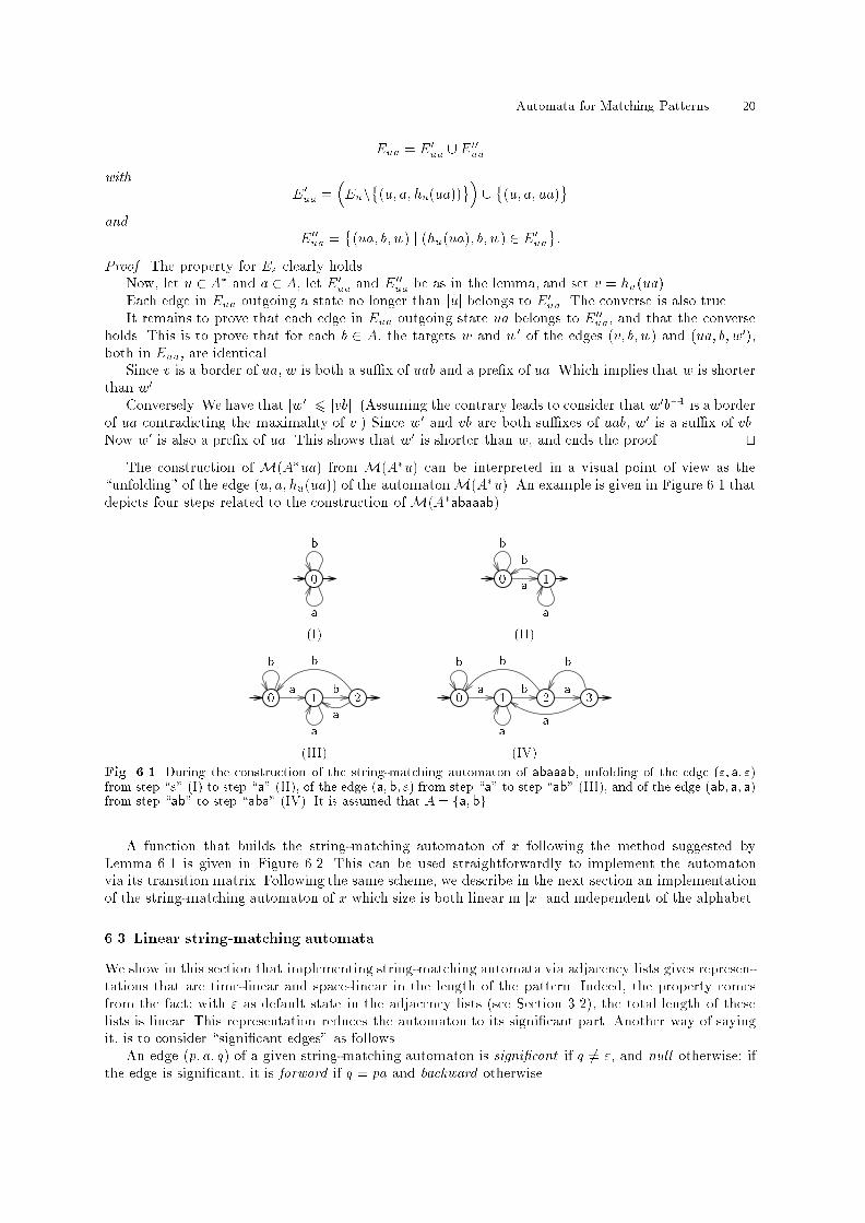
Automata for Matching Patterns 20Eua = E0ua [E00uawith E0ua = �Eun�(u; a; hu(ua))� [ �(u; a; ua)and E00ua = �(ua; b; w) j (hu(ua); b; w) 2 E0ua:Proof. The property for E" clearly holds.Now, let u 2 A� and a 2 A, let E0ua and E00ua be as in the lemma, and set v = hu(ua).Each edge in Eua outgoing a state no longer than juj belongs to E0ua. The converse is also true.It remains to prove that each edge in Eua outgoing state ua belongs to E00ua, and that the converseholds. This is to prove that for each b 2 A, the targets w and w0 of the edges (v; b; w) and (ua; b; w0),both in Eua, are identical.Since v is a border of ua, w is both a su�x of uab and a pre�x of ua. Which implies that w is shorterthan w0.Conversely. We have that jw0j 6 jvbj. (Assuming the contrary leads to consider that w0b�1 is a borderof ua contradicting the maximality of v.) Since w0 and vb are both su�xes of uab, w0 is a su�x of vb.Now w0 is also a pre�x of ua. This shows that w0 is shorter than w, and ends the proof. utThe construction of M(A�ua) from M(A�u) can be interpreted in a visual point of view as the\unfolding" of the edge (u; a; hu(ua)) of the automatonM(A�u). An example is given in Figure 6.1 thatdepicts four steps related to the construction of M(A�abaaab).0ba 0 1ab ab(I) (II)0 1 2a bb ab a 0 1 2 3a b ab ab ba(III) (IV)Fig. 6.1. During the construction of the string-matching automaton of abaaab, unfolding of the edge (";a; ")from step \"" (I) to step \a" (II), of the edge (a;b; ") from step \a" to step \ab" (III), and of the edge (ab; a; a)from step \ab" to step \aba" (IV). It is assumed that A = fa;bg.A function that builds the string-matching automaton of x following the method suggested byLemma 6.1 is given in Figure 6.2. This can be used straightforwardly to implement the automatonvia its transition matrix. Following the same scheme, we describe in the next section an implementationof the string-matching automaton of x which size is both linear in jxj and independent of the alphabet.6.3 Linear string-matching automataWe show in this section that implementing string-matching automata via adjacency lists gives represen-tations that are time-linear and space-linear in the length of the pattern. Indeed, the property comesfrom the fact: with " as default state in the adjacency lists (see Section 3.2), the total length of theselists is linear. This representation reduces the automaton to its signi�cant part. Another way of sayingit, is to consider \signi�cant edges" as follows.An edge (p; a; q) of a given string-matching automaton is signi�cant if q 6= ", and null otherwise; ifthe edge is signi�cant, it is forward if q = pa and backward otherwise.

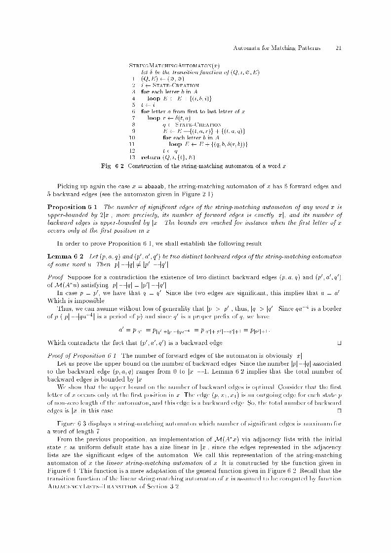
Automata for Matching Patterns 21StringMatchingAutomaton(x)let � be the transition function of (Q; i;?; E)1 (Q;E) (?;?)2 i State-Creation3 for each letter b in A4 loop E E + f(i; b; i)g5 t i6 for letter a from �rst to last letter of x7 loop r �(t; a)8 q State-Creation9 E E � f(t; a; r)g+ f(t; a; q)g10 for each letter b in A11 loop E E + f(q; b; �(r; b))g12 t q13 return (Q; i; ftg; E)Fig. 6.2. Construction of the string-matching automaton of a word x.Picking up again the case x = abaaab, the string-matching automaton of x has 6 forward edges and5 backward edges (see the automaton given in Figure 2.1).Proposition 6.1. The number of signi�cant edges of the string-matching automaton of any word x isupper-bounded by 2jxj; more precisely, its number of forward edges is exactly jxj, and its number ofbackward edges is upper-bounded by jxj. The bounds are reached for instance when the �rst letter of xoccurs only at the �rst position in x.In order to prove Proposition 6.1, we shall establish the following result.Lemma 6.2. Let (p; a; q) and (p0; a0; q0) be two distinct backward edges of the string-matching automatonof some word u. Then jpj � jqj 6= jp0j � jq0j.Proof. Suppose for a contradiction the existence of two distinct backward edges (p; a; q) and (p0; a0; q0)of M(A�u) satisfying jpj � jqj = jp0j � jq0j.In case p = p0, we have that q = q0. Since the two edges are signi�cant, this implies that a = a0.Which is impossible.Thus, we can assume without loss of generality that jpj > jp0j, thus, jqj > jq0j. Since qa�1 is a borderof p (jpj � jqa�1j is a period of p) and since q0 is a proper pre�x of q, we havea0 = pjq0j = pjq0j+jpj�jqa�1j = pjq0j+jp0 j�jq0j+1 = pjp0j+1:Which contradicts the fact that (p0; a0; q0) is a backward edge. utProof of Proposition 6.1. The number of forward edges of the automaton is obviously jxj.Let us prove the upper bound on the number of backward edges. Since the number jpj�jqj associatedto the backward edge (p; a; q) ranges from 0 to jxj � 1, Lemma 6.2 implies that the total number ofbackward edges is bounded by jxj.We show that the upper bound on the number of backward edges is optimal. Consider that the �rstletter of x occurs only at the �rst position in x. The edge (p; x1; x1) is an outgoing edge for each state pof non-zero length of the automaton, and this edge is a backward edge. So, the total number of backwardedges is jxj in this case. utFigure 6.3 displays a string-matching automaton which number of signi�cant edges is maximum fora word of length 7.From the previous proposition, an implementation of M(A�x) via adjacency lists with the initialstate " as uniform default state has a size linear in jxj, since the edges represented in the adjacencylists are the signi�cant edges of the automaton. We call this representation of the string-matchingautomaton of x the linear string-matching automaton of x. It is constructed by the function given inFigure 6.4. This function is a mere adaptation of the general function given in Figure 6.2. Recall that thetransition function of the linear string-matching automaton of x is assumed to be computed by functionAdjacencyLists-Transition of Section 3.2.

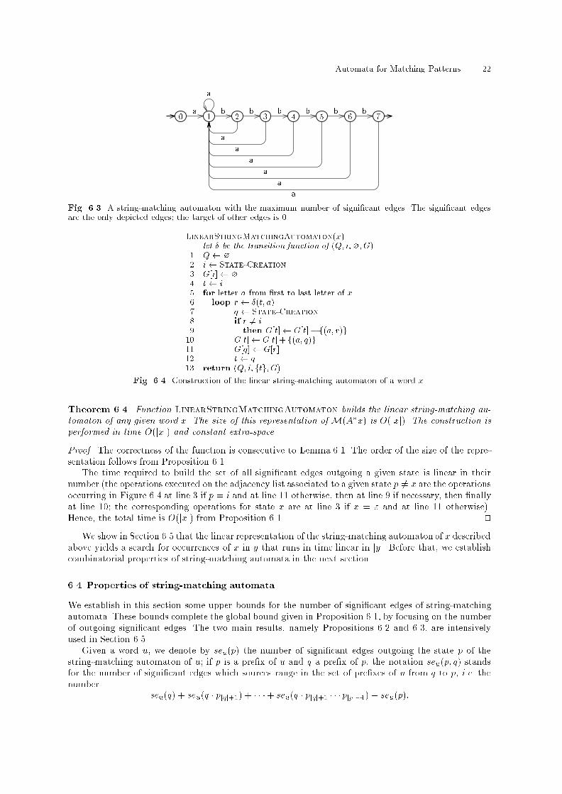
Automata for Matching Patterns 220 1 2 3 4 5 6 7a b b b b b ba a a a a a aFig. 6.3. A string-matching automaton with the maximum number of signi�cant edges. The signi�cant edgesare the only depicted edges; the target of other edges is 0.LinearStringMatchingAutomaton(x)let � be the transition function of (Q; i;?;G)1 Q ?2 i State-Creation3 G[i] ?4 t i5 for letter a from �rst to last letter of x6 loop r �(t; a)7 q State-Creation8 if r 6= i9 then G[t] G[t]� f(a; r)g10 G[t] G[t] + f(a; q)g11 G[q] G[r]12 t q13 return (Q; i; ftg;G)Fig. 6.4. Construction of the linear string-matching automaton of a word x.Theorem 6.4. Function LinearStringMatchingAutomaton builds the linear string-matching au-tomaton of any given word x. The size of this representation of M(A�x) is O(jxj). The construction isperformed in time O(jxj) and constant extra-space.Proof. The correctness of the function is consecutive to Lemma 6.1. The order of the size of the repre-sentation follows from Proposition 6.1.The time required to build the set of all signi�cant edges outgoing a given state is linear in theirnumber (the operations executed on the adjacency list associated to a given state p 6= x are the operationsoccurring in Figure 6.4 at line 3 if p = i and at line 11 otherwise, then at line 9 if necessary, then �nallyat line 10; the corresponding operations for state x are at line 3 if x = " and at line 11 otherwise).Hence, the total time is O(jxj) from Proposition 6.1. utWe show in Section 6.5 that the linear representation of the string-matching automaton of x describedabove yields a search for occurrences of x in y that runs in time linear in jyj. Before that, we establishcombinatorial properties of string-matching automata in the next section.6.4 Properties of string-matching automataWe establish in this section some upper bounds for the number of signi�cant edges of string-matchingautomata. These bounds complete the global bound given in Proposition 6.1, by focusing on the numberof outgoing signi�cant edges. The two main results, namely Propositions 6.2 and 6.3, are intensivelyused in Section 6.5.Given a word u, we denote by seu(p) the number of signi�cant edges outgoing the state p of thestring-matching automaton of u; if p is a pre�x of u and q a pre�x of p, the notation seu(p; q) standsfor the number of signi�cant edges which sources range in the set of pre�xes of u from q to p, i.e. thenumber seu(q) + seu(q � pjqj+1) + � � �+ seu(q � pjqj+1 � � �pjpj�1) + seu(p):

Automata for Matching Patterns 23The next two lemmas provide recurrence relations satis�ed by the numbers seu(p). The expressions arestated using the following notation: given a predicate e, the integer denoted by �(e) has value 1 whene is true, and value 0 otherwise.Lemma 6.3. Let (u; a) 2 A� �A. For each v 2 Pref (ua), we have:seua(v) =8<: seu(Bord(ua)); if v = ua,seu(u) + �(Bord(ua) = "); if v = u,seu(v); otherwise.Proof. This is a straightforward consequence of Lemma 6.1. utLemma 6.4. Let u 2 A+. For each v 2 Pref (u), we have:seu(v) = 8><>: seu(Bord(u)); if v = u,seu(Bord(v)) + �(Bord(va) = "); if va 2 Pref (u)for some a 2 A,1; if v = ".Proof. Follows from Lemma 6.3. utThe next lemma is the \cornerstone" of the proof of the logarithmic bound given in Proposition 6.2stated afterwards.Lemma 6.5. Let u 2 A+. For each v 2 Pref (u)nf"g, we have:2jBord(v)j > jvj =) seu(Bord(v)) = seu(Bord2(v)):Proof. Set k = 2jBord(v)j� jvj, w = v1v2 � � �vk, and a = vk+1. Since wa is a proper border of Bord (v)a,the border of Bord(v)a is nonempty. Then we apply Lemma 6.4 to the proper pre�x Bord (v) of u. utProposition 6.2. Let u 2 A�. For each state p of M(A�u), we have:seu(p) 6 1 + blog2(jpj+ 1)c:Proof. We prove the result by induction on jpj. From Lemma 6.4, this is true if jpj = 0. Next, supposejpj > 1.Let j be the integer such that 2j 6 jpj+ 1 < 2j+1;then let k be the integer such thatjBordk+1(p)j+ 1 < 2j 6 jBordk(p)j+ 1:Let ` 2 f0; : : : ; k � 1g; we have 2jBord`+1(p)j > 2j+1 � 2 > jpj > jBord`(p)j; which impliesseu(Bord`+1(p)) = seu(Bord`+2(p)) from Lemma 6.5. Hence we get the equalityseu(Bord(p)) = seu(Bordk+1(p)):From the induction hypothesis applied to the state Bordk+1(p), we getseu(Bordk+1(p)) 6 1 + blog2(jBordk+1(p)j+ 1)c:Now Lemma 6.4 implies seu(p) 6 seu(Bord (p)) + 1:This shows that seu(p) 6 j + 1 = 1 + blog2(jpj+ 1)c;and ends the proof. ut

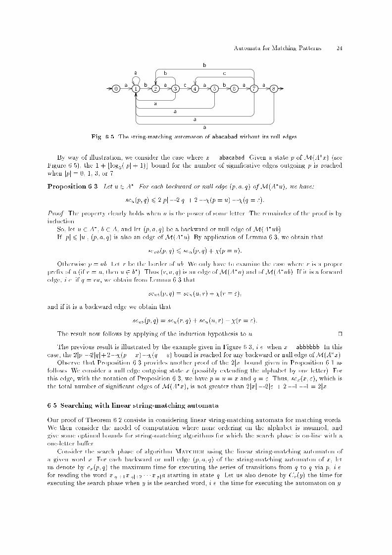
Automata for Matching Patterns 240 1 2 3 4 5 6 7 8a b a c a b a aa a a a ab b cFig. 6.5. The string-matching automaton of abacabad without its null edges.By way of illustration, we consider the case where x = abacabad. Given a state p of M(A�x) (seeFigure 6.5), the 1 + blog2(jpj + 1)c bound for the number of signi�cative edges outgoing p is reachedwhen jpj = 0, 1, 3, or 7.Proposition 6.3. Let u 2 A�. For each backward or null edge (p; a; q) of M(A�u), we have:seu(p; q) 6 2jpj � 2jqj+ 2� �(p = u)� �(q = "):Proof. The property clearly holds when u is the power of some letter. The remainder of the proof is byinduction.So, let u 2 A�, b 2 A, and let (p; a; q) be a backward or null edge of M(A�ub).If jpj 6 juj, (p; a; q) is also an edge of M(A�u). By application of Lemma 6.3, we obtain thatseub(p; q) 6 seu(p; q) + �(p = u):Otherwise p = ub. Let r be the border of ub. We only have to examine the case where r is a properpre�x of u (if r = u, then u 2 b�). Thus (r; a; q) is an edge ofM(A�u) and ofM(A�ub). If it is a forwardedge, i.e. if q = ra, we obtain from Lemma 6.3 thatseub(p; q) = seu(u; r) + �(r = ");and if it is a backward edge we obtain thatseub(p; q) = seu(r; q) + seu(u; r) + �(r = "):The result now follows by applying of the induction hypothesis to u. utThe previous result is illustrated by the example given in Figure 6.3, i.e. when x = abbbbbb. In thiscase, the 2jpj�2jqj+2��(p = x)��(q = ") bound is reached for any backward or null edge ofM(A�x).Observe that Proposition 6.3 provides another proof of the 2jxj bound given in Proposition 6.1 asfollows. We consider a null edge outgoing state x (possibly extending the alphabet by one letter). Forthis edge, with the notation of Proposition 6.3, we have p = u = x and q = ". Thus, sex(x; "), which isthe total number of signi�cant edges of M(A�x), is not greater than 2jxj � 2j"j+ 2� 1� 1 = 2jxj.6.5 Searching with linear string-matching automataOur proof of Theorem 6.2 consists in considering linear string-matching automata for matching words.We then consider the model of computation where none ordering on the alphabet is assumed, andgive some optimal bounds for string-matching algorithms for which the search phase is on-line with aone-letter bu�er.Consider the search phase of algorithm Matcher using the linear string-matching automaton ofa given word x. For each backward or null edge (p; a; q) of the string-matching automaton of x, letus denote by cx(p; q) the maximum time for executing the series of transitions from q to q via p, i.e.for reading the word xjqj+1xjqj+2 � � �xjpja starting in state q. Let us also denote by Cx(y) the time forexecuting the search phase when y is the searched word, i.e. the time for executing the automaton on y.

Automata for Matching Patterns 25Lemma 6.6. Let x; y 2 A�. There exists a �nite sequence of backward or null edges of M(A�x), say((pj ; aj; qj))16j6k, satisfying the three following conditions:(i) qk = ";(ii) Pkj=1�jpjj � jqjj+ 1� = jyj;(iii) Cx(y) 6Pkj=1 cx(pj; qj).Proof. The proof is by induction on jyj. Since the property trivially holds when jyj = 0, we assume thatjyj > 1.Observe �rst that since an upper bound is expected for Cx(y), we can assume, even if the alphabethas to be extended by one letter, that the last letter of y is not a letter occurring actually in x. Hence,we can assume that the lastly performed transition corresponds to a null edge.Now, let (p`)06`6jyj be the sequence of successive values of the current state p of algorithmMatcher(in other words p` = hx(y1y2 � � �y`)). Let m, 0 6 m 6 jyj � 1, be the minimal integer satisfyingpm+1 = pm0 for some m0 6 m, then let m0 be the integer in f0; : : : ;mg such that pm0 = pm+1. Thus,the triple (pm; ym+1; pm0) is a backward or null edge of M(A�x), and the m�m0 + 1 successive lettersym0+1, ym0+2, : : : , ym+1 of y have been read during the computation of the transitions from pm0 to pm+1via pm. Consider the word y0 de�ned by y0 = y1y2 � � �ym0 � ym+2ym+3 � � �yjyj. Following the de�nition ofm and m0 we have that Cx(y) 6 cx(pm; pm0) + Cx(y0). Applying the induction hypothesis to y0 givesthe existence of a �nite sequence e0 as depicted in the statement. The expected sequence related to ycan then be obtained by adding the edge ((pm; ym+1; pm0)) in front of the sequence e0. It clearly satis�esconditions (i) to (iii). This ends the proof. utTheorem 6.5. Let x and y be words. Using the linear string-matching automaton of x, searching forall occurrences of x as factors of y (search phase of algorithm Matcher) is performed in time O(jyj),constant extra-space, within a delay O(logminf1 + blog2 jxjc; card(A)g).Proof. Whatever e�cient is the implementation of adjacency lists, we may assume that the time forexecuting the transition from the current state by the current input letter is asymptotically linear inthe number of signi�cant edges outgoing the involved state. For each backward or null edge (p; a; q) ofM(A�x), this assumption implies that cx(p; q) = O(sex(p; q));which leads to cx(p; q) = O(jpj � jqj+ 1);by application of Proposition 6.3. We �nally apply Lemma 6.6, and get the O(jyj) bound.We now turn to the proof of the delay. The cardinality of each adjacency list is both upper-boundedby card(A), and, from Lemma6.3 and Proposition 6.2, by 1+blog2 jxjc. Now, observe that each adjacencylist can be arranged in a balanced tree when computing it, without loosing the linear-time complexityof the construction. This provides a logarithmic time for computing a transition. Which proves theasymptotic bound of the delay. utIn the remainder of the section, no ordering on the alphabet is assumed, contrary to what is assumedfor the previous statement. The model of computation is the comparison model in which algorithms haveaccess to the input words by comparing pairs of letters to test whether they are equal or not. Withinthis model, given a word x, we denote by S(x) the family of the string-matching algorithms for whichthe search phase is on-line with a one-letter bu�er.String-matching algorithms based on the linear string-matching automaton of x can be classi�edaccording to the way the adjacency lists are ordered or scanned. For example, the adjacency lists can beordered by decreasing length of target, or by the frequency of labels as letters of the pre�x already read;each adjacency list can also be scanned according to a random processing. (Let us observe that any ofthese variations preserves the linear time of the search). We denote by L(x) the subfamily of algorithmsin S(x) which use the linear string-matching automaton of x to search a given word for occurrences ofx.

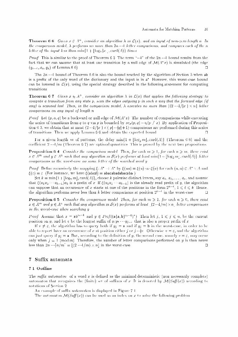
Automata for Matching Patterns 26Theorem 6.6. Given x 2 A+, consider an algorithm � in L(x), and an input of non-zero length n. Inthe comparison model, � performs no more than 2n� 1 letter comparisons, and compares each of the nletter of the input less than minf1 + blog2 jxjc; card(A)g times.Proof. This is similar to the proof of Theorem 6.5. The term \�1" of the 2n� 1 bound results from thefact that we can assume that at least one transition by a null edge of M(A�x) is simulated (the edge(qk�1; ak; qk) of Lemma 6.6). utThe 2n� 1 bound of Theorem 6.6 is also the bound reached by the algorithm of Section 5 when abis a pre�x of the only word of the dictionary and the input is in a�. However, this worst-case boundcan be lowered in L(x), using the special strategy described in the following statement for computingtransitions.Theorem 6.7. Given x 2 A+, consider an algorithm � in L(x) that applies the following strategy: tocompute a transition from any state p, scan the edges outgoing p in such a way that the forward edge (ifany) is scanned last. Then, in the comparison model, � executes no more than b(2 � 1=jxj)� nc lettercomparisons on any input of length n.Proof. Let (p; a; q) be a backward or null edge of M(A�x). The number of comparisons while executingthe series of transitions from q to q via p is bounded by sex(p; q)� �(p 6= x). By application of Proposi-tion 6.3, we obtain that at most (2�1=jxj)� (jpj� jqj+1) comparisons are performed during this seriesof transitions. Then we apply Lemma 6.6 and obtain the expected bound. utFor a given length m of patterns, the delay minf1 + blog2mc; card(A)g (Theorem 6.6) and thecoe�cient 2� 1=m (Theorem 6.7) are optimal quantities. This is proved by the next two propositions.Proposition 6.4. Consider the comparison model. Then, for each m > 1, for each n > m, there existx 2 Am and y 2 An such that any algorithm in S(x) performs at least minf1+ blog2mc; card(A)g lettercomparisons in the worst-case on some letter of the searched word y.Proof. De�ne recursively the mapping �:A� ! A� by �(ua) = �(u) �a � �(u) for each (u; a) 2 A��A and�(") = ". (For instance, we have �(abcd) = abacabadabacaba.)Set k = minf1+blog2mc; card(A)g, choose k pairwise distinct letters, say a1, a2, : : : , ak, and assumethat �(a1a2 � � �ak�1)ak is a pre�x of x. If �(a1a2 � � �ak�1) is the already read pre�x of y, the algorithmcan suppose that an occurrence of x starts at one of the positions in the form 2k�`, 1 6 ` 6 k. Hence,the algorithm performs never less than k letter comparisons at position 2k�1 in the worst-case. utProposition 6.5. Consider the comparison model. Then, for each m > 1, for each n > 0, there existx 2 Am and y 2 An such that any algorithm in S(x) performs at least b(2�1=m)�nc letter comparisonsin the worst-case when searching y.Proof. Assume that x = abm�1 and y 2 Pref ((afa; bgm�1)�). Then let j, 1 6 j 6 n, be the currentposition on y, and let v be the longest su�x of y1y2 � � �yj�1 that is also a proper pre�x of x.If v 6= ", the algorithm has to query both if yj = a and if yj = b in the worst-case, in order to beable to report later an occurrence of x at position either j or j�jvj. Otherwise v = ", and the algorithmcan just query if yj = a. But, according to the de�nition of y, the second case, namely v = ", may occuronly when j � 1 (modm). Therefore, the number of letter comparisons performed on y is then neverless than 2n� dn=me = b(2 � 1=m) � nc in the worst-case. ut7. Su�x automata7.1 OutlineThe su�x automaton of a word x is de�ned as the minimal deterministic (non necessarily complete)automaton that recognizes the (�nite) set of su�xes of x. It is denoted by M(Su� (x)) according tonotations of Section 2.An example of su�x automaton is displayed in Figure 7.1.The automatonM(Su� (x)) can be used as an index on x to solve the following problem.

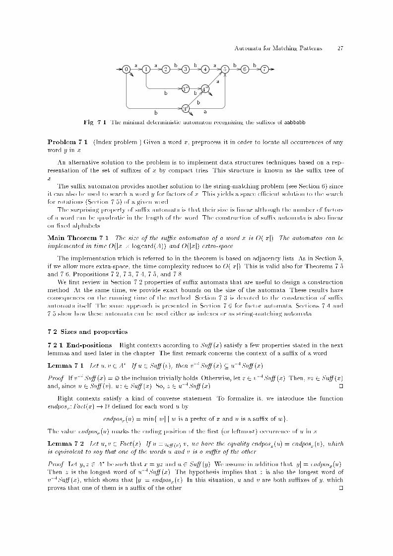
Automata for Matching Patterns 270 1 2 3 4 5 6 730300 400a a b b a b bb b ab b aFig. 7.1. The minimal deterministic automaton recognizing the su�xes of aabbabb.Problem 7.1. (Index problem.) Given a word x, preprocess it in order to locate all occurrences of anyword y in x.An alternative solution to the problem is to implement data structures techniques based on a rep-resentation of the set of su�xes of x by compact tries. This structure is known as the su�x tree ofx. The su�x automaton provides another solution to the string-matching problem (see Section 6) sinceit can also be used to search a word y for factors of x. This yields a space e�cient solution to the searchfor rotations (Section 7.5) of a given word.The surprising property of su�x automata is that their size is linear although the number of factorsof a word can be quadratic in the length of the word. The construction of su�x automata is also linearon �xed alphabets.Main Theorem 7.1. The size of the su�x automaton of a word x is O(jxj). The automaton can beimplemented in time O(jxj � log card(A)) and O(jxj) extra-space.The implementation which is referred to in the theorem is based on adjacency lists. As in Section 5,if we allow more extra-space, the time complexity reduces to O(jxj). This is valid also for Theorems 7.5and 7.6, Propositions 7.2, 7.3, 7.4, 7.5, and 7.8.We �rst review in Section 7.2 properties of su�x automata that are useful to design a constructionmethod. At the same time, we provide exact bounds on the size of the automata. These results haveconsequences on the running time of the method. Section 7.3 is devoted to the construction of su�xautomata itself. The same approach is presented in Section 7.6 for factor automata. Sections 7.4 and7.5 show how these automata can be used either as indexes or as string-matching automata.7.2 Sizes and properties7.2.1 End-positions. Right contexts according to Su� (x) satisfy a few properties stated in the nextlemmas and used later in the chapter. The �rst remark concerns the context of a su�x of a word.Lemma 7.1. Let u; v 2 A�. If u 2 Su� (v), then v�1Su� (x) � u�1Su� (x).Proof. If v�1Su� (x) = ? the inclusion trivially holds. Otherwise, let z 2 v�1Su� (x). Then, vz 2 Su� (x)and, since u 2 Su� (v), uz 2 Su� (x). So, z 2 u�1Su� (x). utRight contexts satisfy a kind of converse statement. To formalize it, we introduce the functionendposx:Fact(x)! N de�ned for each word u byendposx(u) = minfjwj j w is a pre�x of x and u is a su�x of wg:The value endposx(u) marks the ending position of the �rst (or leftmost) occurrence of u in x.Lemma 7.2. Let u; v 2 Fact(x). If u �Su� (x) v, we have the equality endposx(u) = endposx(v), whichis equivalent to say that one of the words u and v is a su�x of the other.Proof. Let y; z 2 A� be such that x = yz and u 2 Su� (y). We assume in addition that jyj = endposx(u).Then z is the longest word of u�1Su� (x). The hypothesis implies that z is also the longest word ofv�1Su� (x), which shows that jyj = endposx(v). In this situation, u and v are both su�xes of y, whichproves that one of them is a su�x of the other. ut

Automata for Matching Patterns 28Another often used property of the syntactic congruence associated with Su� (x) is that it partitionsthe su�xes of factors into intervals (with respect to the lengths of su�xes).Lemma 7.3. Let u; v; w 2 Fact(x). Then, if u 2 Su� (v), v 2 Su� (w), and u �Su� (x) w, we haveu �Su� (x) v �Su� (x) w.Proof. By Lemma 7.1, we have the inclusions w�1Su� (x) � v�1Su� (x) � u�1Su� (x). But then, theequality u�1Su� (x) = w�1Su� (x) implies the conclusion of the statement. utA consequence of the next property is that the direct inclusion of right contexts relative to Su� (x)induces a tree structure on them. In the tree, the parent link corresponds to the proper direct inclusion.This link is discussed in Section 7.2.2 where it is called the \su�x function".Corollary 7.1. Let u; v 2 A�. Then, one of the three following conditions holds:(i) u�1Su� (x) � v�1Su� (x);(ii) v�1Su� (x) � u�1Su� (x);(iii) u�1Su� (x) \ v�1Su� (x) = ?.Proof. We just have to show that if u�1Su� (x) \ v�1Su� (x) 6= ?, then we have the inclusionu�1Su� (x) � v�1Su� (x) or the inclusion v�1Su� (x) � u�1Su� (x). Let z 2 u�1Su� (x) \ v�1Su� (x).Then, uz and vz are su�xes of x. So, u and v are su�xes of xz�1, which implies that one of the wordsu and v is a su�x of the other. Therefore, the conclusion follows by Lemma 7.1. ut7.2.2 Su�x function. We consider the function sx:Fact(x) ! Fact(x) de�ned for each nonemptyword v in Fact(x) by sx(v) = the longest u 2 Su� (v) such that u 6�Su� (x) v:Regarding Lemma 7.1, this is equivalent tosx(v) = the longest u 2 Su� (v) such that v�1Su� (x) � u�1Su� (x):The function sx is called the su�x function relative to x. An obvious consequence of the de�nition isthat sx(v) is a proper su�x of v. The next lemma shows that the su�x function sx induces what wecall a \su�x link" on states ofM(Su� (x)).Lemma 7.4. Assuming x 6= ", let u; v 2 Fact(x)nf"g. If u �Su� (x) v, then sx(u) = sx(v).Proof. FromLemma7.2 we can assume without loss of generality that u 2 Su� (v). The word u cannot bea su�x of sx(v), because Lemma 7.3 would then imply sx(v)�1Su� (x) = v�1Su� (x), which contradictsthe de�nition of sx(v). Therefore, sx(v) is a su�x of u. Since, by de�nition, it is the longest su�x of vnon equivalent to it, it is equal to sx(u). utLemma 7.5. If x 6= ", sx(x) is the longest su�x of x that occurs at least twice in x.Proof. The set x�1Su� (x) is equal to f"g. Since x and sx(x) are not equivalent, the set sx(x)�1Su� (x)contains some nonempty word z. Therefore, sx(x)z and sx(x) are su�xes of x, which proves that sx(x)occurs at least twice in x. Any su�x w of x, longer than sx(x), satis�es w�1Su� (x) = x�1Su� (x) = f"gby de�nition of sx(x). Thus, w occurs only as a su�x of x, which ends the proof. utThe next lemma shows that the image of a factor of x by the su�x function is a word of maximumlength in its own congruence class. This fact is needed in Section 7.5 where the su�x automaton is usedas a matching automaton.Lemma 7.6. Assuming x 6= ", let u 2 Fact(x)nf"g. Then, any word equivalent to sx(u) is a su�x ofsx(u).Proof. Let w = sx(u) and v �Su� (x) sx(u). The word w is a proper su�x of u. If the conclusion of thestatement is false, Lemma 7.2 insures that w is a proper su�x of v. Let z 2 u�1Su� (x). Since w is asu�x of u and is equivalent to v, we have z 2 w�1Su� (x) = v�1Su� (x). Therefore, u and v are bothsu�xes of xz�1, which implies that one of them is a su�x of the other. But this contradicts either thede�nition of w, or the conclusion of Lemma 7.3. This proves that v is necessarily a su�x of w. ut

Automata for Matching Patterns 297.2.3 State splitting. In this section we present the properties that yield to the on-line construction ofsu�x automata described in Section 7.3. This is achieved by deriving relations between the congruences�Su� (w) and �Su� (wa) for any couple (w; a) 2 A� �A. The �rst property, stated in Lemma 7.8, is that�Su� (wa) is a re�nement of �Su� (w). The next lemma shows how right contexts evolves.Lemma 7.7. Let w 2 A� and a 2 A. For each u 2 A�, we have:u�1Su� (wa) = �u�1Su� (w)a [ f"g; if u 2 Su� (wa),u�1Su� (w)a; otherwise.Proof. Note �rst that " 2 u�1Su� (wa) is equivalent to u 2 Su� (wa). So, it remains to proveu�1Su� (wa)nf"g = u�1Su� (w)a.Let z be a nonempty word in u�1Su� (wa). This means uz 2 Su� (wa). The word uz can then bewritten uz0a with uz0 2 Su� (w). Thus, z0 2 u�1Su� (w), and z 2 u�1Su� (w)a.Conversely. Let z be a (nonempty) word in u�1Su� (w)a. It can be written z0a for some z0 2u�1Su� (w). Therefore, uz0 2 Su� (w), which implies uz = uz0a 2 Su� (wa), that is z 2 u�1Su� (wa).utLemma 7.8. Let w 2 A� and a 2 A. The congruence �Su� (wa) is a re�nement of the congruence�Su� (w), that is, for each u; v 2 A�, u �Su� (wa) v implies u �Su� (w) v.Proof. We assume u �Su� (wa) v, that is, u�1Su� (wa) = v�1Su� (wa), and prove u �Su� (w) v, that is,u�1Su� (w) = v�1Su� (w). We only show that u�1Su� (w) � v�1Su� (w) because the reverse inclusionfollows by symmetry.If u�1Su� (w) is empty, the inclusion trivially holds. Otherwise, let z 2 u�1Su� (w). This is equivalentto uz 2 Su� (w), which implies uza 2 Su� (wa). The hypothesis gives vza 2 Su� (wa), and thusvz 2 Su� (w) or z 2 v�1Su� (w), which achieves the proof. utGiven a word w, the congruence �Su� (w) partitions A� into classes. And Lemma 7.8 remains to saythat these classes are union of classes according to �Su� (wa), a 2 A. It turns out that only one or twoclasses according to �Su� (w) split into two sub-classes to get the partition induced by �Su� (wa). One ofthe class that splits is the class of words not occurring in w. It contains the word wa itself that gives riseto a new class and a new state of the su�x automaton (see Lemma 7.9). Theorem 7.2 and its corollariesexhibit conditions under which another class also splits and how it splits.Lemma 7.9. Let w 2 A� and a 2 A. Let z be the longest su�x of wa occurring in w. If u is a su�x ofwa such that juj > jzj, u �Su� (wa) wa.Proof. This is a straightforward consequence of Lemma 7.5. utTheorem 7.2. Let w 2 A� and a 2 A. Let z be the longest su�x of wa occurring in w. Let z0 be thelongest factor of w such that z0 �Su� (w) z. For each u; v 2 Fact(w), we have:u �Su� (w) v and u 6�Su� (w) z =) u �Su� (wa) v:Furthermore, for each u 2 A�, we have:u �Su� (w) z =) �u �Su� (wa) z; if juj 6 jzj,u �Su� (wa) z0; otherwise.Proof. Let u; v 2 Fact(w) be such that u �Su� (w) v, that is, u�1Su� (w) = v�1Su� (w). We �rst assumeu 6�Su� (w) z and prove u �Su� (wa) v, that is u�1Su� (wa) = v�1Su� (wa).By Lemma 7.7, we just have to prove that u 2 Su� (wa) is equivalent to v 2 Su� (wa). Indeed, it iseven su�cient to prove that u 2 Su� (wa) implies v 2 Su� (wa) because the reverse implication comesby symmetry.Assume then that u 2 Su� (wa). Since u 2 Fact(w), u is a su�x of z, by de�nition of z. So, we canconsider the largest integer k > 0 such that juj 6 jswk(z)j. Note that swk(z) is a su�x of wa (as z is),and that Lemma 7.3 insures that u �Su� (w) swk(z). So, v �Su� (w) swk(z) by transitivity.

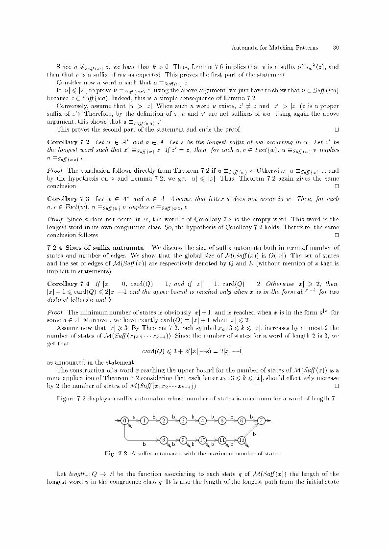
Automata for Matching Patterns 30Since u 6�Su� (w) z, we have that k > 0. Thus, Lemma 7.6 implies that v is a su�x of swk(z), andthen that v is a su�x of wa as expected. This proves the �rst part of the statement.Consider now a word u such that u �Su� (w) z.If juj 6 jzj, to prove u �Su� (wa) z, using the above argument, we just have to show that u 2 Su� (wa)because z 2 Su� (wa). Indeed, this is a simple consequence of Lemma 7.2.Conversely, assume that juj > jzj. When such a word u exists, z0 6= z and jz0j > jzj (z is a propersu�x of z0). Therefore, by the de�nition of z, u and z0 are not su�xes of wa. Using again the aboveargument, this shows that u �Su� (wa) z0.This proves the second part of the statement and ends the proof. utCorollary 7.2. Let w 2 A� and a 2 A. Let z be the longest su�x of wa occurring in w. Let z0 bethe longest word such that z0 �Su� (w) z. If z0 = z, then, for each u; v 2 Fact(w), u �Su� (w) v impliesu �Su� (wa) v.Proof. The conclusion follows directly from Theorem 7.2 if u 6�Su� (w) z. Otherwise, u �Su� (w) z, andby the hypothesis on z and Lemma 7.2, we get juj 6 jzj. Thus, Theorem 7.2 again gives the sameconclusion. utCorollary 7.3. Let w 2 A� and a 2 A. Assume that letter a does not occur in w. Then, for eachu; v 2 Fact(w), u �Su� (w) v implies u �Su� (wa) v.Proof. Since a does not occur in w, the word z of Corollary 7.2 is the empty word. This word is thelongest word in its own congruence class. So, the hypothesis of Corollary 7.2 holds. Therefore, the sameconclusion follows. ut7.2.4 Sizes of su�x automata. We discuss the size of su�x automata both in term of number ofstates and number of edges. We show that the global size of M(Su� (x)) is O(jxj). The set of statesand the set of edges ofM(Su� (x)) are respectively denoted by Q and E (without mention of x that isimplicit in statements).Corollary 7.4. If jxj = 0, card(Q) = 1; and if jxj = 1, card(Q) = 2. Otherwise jxj > 2; then,jxj+ 1 6 card(Q) 6 2jxj � 1 and the upper bound is reached only when x is in the form abjxj�1 for twodistinct letters a and b.Proof. The minimum number of states is obviously jxj+1, and is reached when x is in the form ajxj forsome a 2 A. Moreover, we have exactly card(Q) = jxj+ 1 when jxj 6 2.Assume now that jxj > 3. By Theorem 7.2, each symbol xk, 3 6 k 6 jxj, increases by at most 2 thenumber of states of M(Su� (x1x2 � � �xk�1)). Since the number of states for a word of length 2 is 3, weget that card(Q) 6 3 + 2(jxj � 2) = 2jxj � 1;as announced in the statement.The construction of a word x reaching the upper bound for the number of states ofM(Su� (x)) is amere application of Theorem 7.2 considering that each letter xk, 3 6 k 6 jxj, should e�ectively increaseby 2 the number of states of M(Su� (x1x2 � � �xk�1)). utFigure 7.2 displays a su�x automaton whose number of states is maximum for a word of length 7.0 1 2 3 4 5 6 78 9 10 11 12a b b b b b bb b b b b bFig. 7.2. A su�x automaton with the maximum number of states.Let lengthx:Q ! N be the function associating to each state q of M(Su� (x)) the length of thelongest word u in the congruence class q. It is also the length of the longest path from the initial state

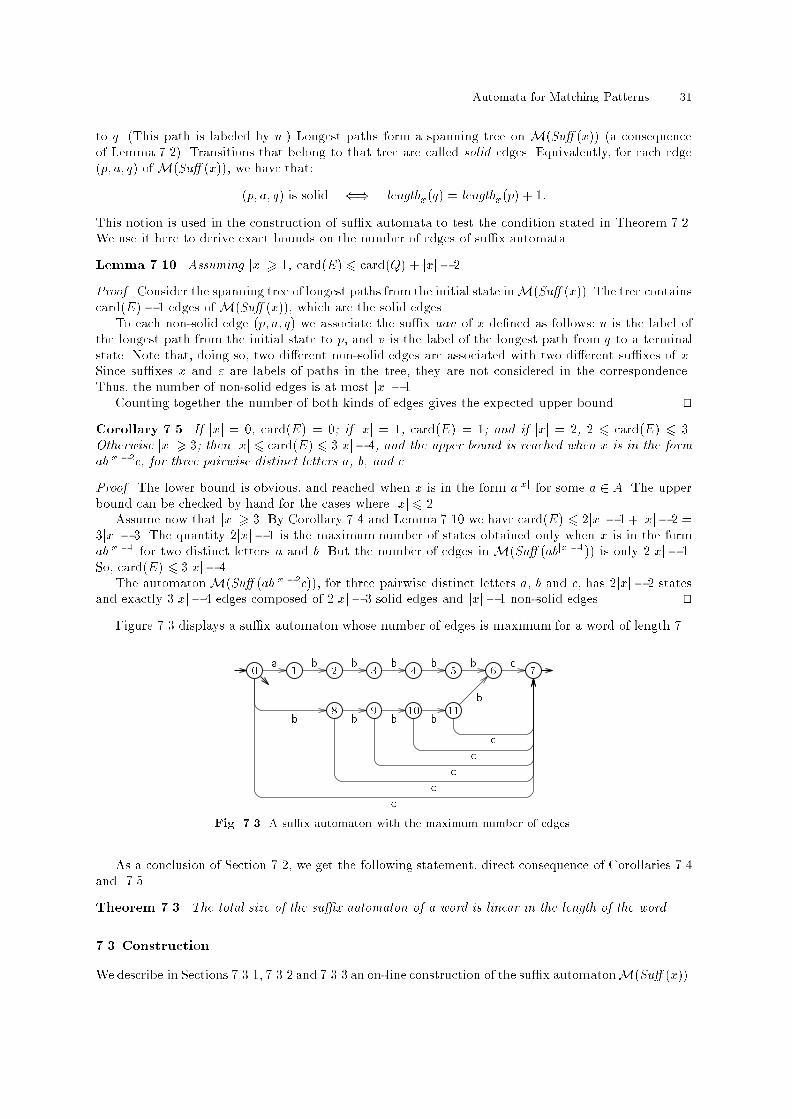
Automata for Matching Patterns 31to q. (This path is labeled by u.) Longest paths form a spanning tree on M(Su� (x)) (a consequenceof Lemma 7.2). Transitions that belong to that tree are called solid edges. Equivalently, for each edge(p; a; q) ofM(Su� (x)), we have that:(p; a; q) is solid () lengthx(q) = lengthx(p) + 1:This notion is used in the construction of su�x automata to test the condition stated in Theorem 7.2.We use it here to derive exact bounds on the number of edges of su�x automata.Lemma 7.10. Assuming jxj > 1, card(E) 6 card(Q) + jxj � 2.Proof. Consider the spanning tree of longest paths from the initial state inM(Su� (x)). The tree containscard(E) � 1 edges ofM(Su� (x)), which are the solid edges.To each non-solid edge (p; a; q) we associate the su�x uav of x de�ned as follows: u is the label ofthe longest path from the initial state to p, and v is the label of the longest path from q to a terminalstate. Note that, doing so, two di�erent non-solid edges are associated with two di�erent su�xes of x.Since su�xes x and " are labels of paths in the tree, they are not considered in the correspondence.Thus, the number of non-solid edges is at most jxj � 1.Counting together the number of both kinds of edges gives the expected upper bound. utCorollary 7.5. If jxj = 0, card(E) = 0; if jxj = 1, card(E) = 1; and if jxj = 2, 2 6 card(E) 6 3.Otherwise jxj > 3; then jxj 6 card(E) 6 3jxj � 4, and the upper bound is reached when x is in the formabjxj�2c, for three pairwise distinct letters a, b, and c.Proof. The lower bound is obvious, and reached when x is in the form ajxj for some a 2 A. The upperbound can be checked by hand for the cases where jxj 6 2.Assume now that jxj > 3. By Corollary 7.4 and Lemma 7.10 we have card(E) 6 2jxj� 1 + jxj � 2 =3jxj � 3. The quantity 2jxj � 1 is the maximum number of states obtained only when x is in the formabjxj�1 for two distinct letters a and b. But the number of edges in M(Su� (abjxj�1)) is only 2jxj � 1.So, card(E) 6 3jxj � 4.The automatonM(Su� (abjxj�2c)), for three pairwise distinct letters a, b and c, has 2jxj � 2 statesand exactly 3jxj � 4 edges composed of 2jxj � 3 solid edges and jxj � 1 non-solid edges. utFigure 7.3 displays a su�x automaton whose number of edges is maximum for a word of length 7.0 1 2 3 4 5 6 78 9 10 11a b b b b b cb b b b bc ccccFig. 7.3. A su�x automaton with the maximum number of edges.As a conclusion of Section 7.2, we get the following statement, direct consequence of Corollaries 7.4and 7.5.Theorem 7.3. The total size of the su�x automaton of a word is linear in the length of the word.7.3 ConstructionWe describe in Sections 7.3.1, 7.3.2 and 7.3.3 an on-line construction of the su�x automatonM(Su� (x)).

Automata for Matching Patterns 327.3.1 Su�x links and su�x paths. The construction of M(Su� (x)) follows Theorem 7.2 andits corollaries stated in Section 7.2. Conditions that appear in these statements are checked on theautomaton with the help of a function de�ned on its states and called the \su�x link". It is a failurefunction in the sense of Section 3.4, and is used with this purpose in Section 7.5.Let (Q; i; T;E) = M(Su� (x)) and � be the corresponding transition function. Let p 2 Qnfig. Statep is a class of factors of x congruent with respect to �Su� (x). Let u be any word in the class of p (u 6= "because p 6= i). Then, the su�x link of p is the congruence class of sx(u). By Lemma 7.4 the value sx(u)is independent of the word u chosen in the class p, which makes the de�nition coherent. We denote byfx the function assignating to each state p its congruence class sx(u).Su�x links induce by iteration \su�x paths" in M(Su� (x)). Note that if q = fx(p), thenlengthx(q) < lengthx(p). Therefore, the sequence(p; fx(p); fx2(p); : : :)is �nite and ends with the initial state i. It is called the su�x path of p.We denote by lastx the state of M(Su� (x)) that is the class of x itself. State lastx has no outgoingedge (otherwise M(Su� (x)) would recognize words longer than x). The su�x path of lastx, i.e.(lastx; fx(lastx); fx2(lastx); : : :);plays an important role in the on-line construction. It is used to test e�ciently conditions appearing instatements of the previous section.Proposition 7.1. Let u 2 Fact(x)nf"g and set p = �(i; u). Then, for any integer k > 0 for whichsxk(u) is de�ned, fxk(p) = �(i; sxk(u)).Proof. The proof is by induction on k.For k = 0, the equality holds by hypothesis.Next, let k > 1 such that sxk(u) is de�ned and assume that fxk�1(p) = �(i; sxk�1(u)). By de�nitionof fx, fx(fxk�1(p)) is the congruence class of the word sx(sxk�1(u)). Therefore, fxk(p) = �(i; sxk(u)) asexpected. utCorollary 7.6. Terminal states of M(Su� (x)), the states in T , are exactly the states of the su�x pathof state lastx.Proof. Let p be a state of the su�x path of lastx. Then, p = fxk(lastx) for some integer k > 0. ByProposition 7.1, since lastx = �(i; x), we have p = �(i; sxk(x)). Since sxk(x) is a su�x of x, p 2 T .Conversely, let p 2 T . So, for some u 2 Su� (x), p = �(i; u). Since u 2 Su� (x), we can considerthe largest integer k > 0 such that juj 6 jsxk(x)j. By Lemma 7.3 we get u �Su� (x) sxk(x). Thus, p =�(i; sxk(x)) by de�nition of M(Su� (x)). Then, Proposition 7.1 applied to x shows that p = fxk(lastx),which proves that p belongs to the su�x path of lastx. ut7.3.2 On-line construction. This section presents an on-line construction of su�x automata. Ateach stage of the construction, just after processing a pre�x x1x2 � � �x` of x, the su�x automatonM(Su� (x1x2 � � �x`)) is built. Terminal states are implicitly known by the su�x path of lastx1x2 ���x` (seeCorollary 7.6). The state lastx1x2���x` is explicitly represented by a variable in the function building theautomaton.Two other elements are also used: Length and F . The table Length represents the function lengthxde�ned on states of the automaton. All edges are solid or non-solid according to the de�nition ofSection 7.2 that relies on function lengthx. Su�x links of states (di�erent from the initial state) arestored in a table denoted by F that stands for the function fx. The implementation ofM(Su� (x)) withthese extra features is discussed in the next section.The on-line construction in Figure 7.4 is based on procedure SA-Extend given in Figure 7.5. Thelatter procedure processes the next letter, say x`, of the word x. It transforms the su�x automatonM(Su� (x1x2 � � �x`�1)) already built into the su�x automaton M(Su� (x1x2 � � �x`)).We illustrate how procedure SA-Extend processes the current automaton through three examples.Let us consider that x1x2 � � �x`�1 = ccccbbccc, and let us examine three possible cases according to

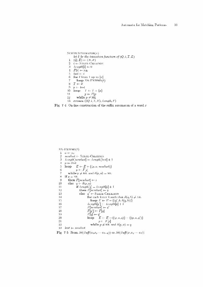
Automata for Matching Patterns 33SuffixAutomaton(x)let � be the transition function of (Q; i; T;E)1 (Q;E) (?;?)2 i State-Creation3 Length[i] 04 F [i] nil5 last i6 for ` from 1 up to jxj7 loop SA-Extend(`)8 T ?9 p last10 loop T T + fpg11 p F [p]12 while p 6= nil13 return ((Q; i; T;E);Length; F )Fig. 7.4. On-line construction of the su�x automaton of a word x.SA-Extend(`)1 a x`2 newlast State-Creation3 Length[newlast] Length[last] + 14 p last5 loop E E + f(p; a; newlast)g6 p F [p]7 while p 6= nil and �(p; a) = nil8 if p = nil9 then F [newlast] i10 else q �(p; a)11 if Length[q] = Length[p] + 112 then F [newlast] q13 else q0 State-Creation14 for each letter b such that �(q; b) 6= nil15 loop E E + f(q0; b; �(q; b))g16 Length[q0] Length[p] + 117 F [newlast] q018 F [q0] F [q]19 F [q] q020 loop E E � f(p; a; q)g+ f(p; a; q0)g21 p F [p]22 while p 6= nil and �(p; a) = q23 last newlastFig. 7.5. FromM(Su� (x1x2 � � �x`�1)) toM(Su� (x1x2 � � �x`)).

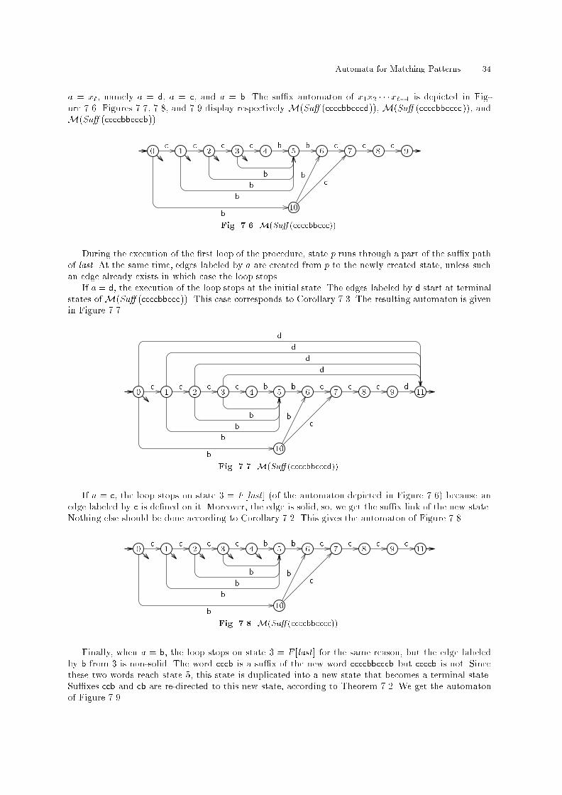
Automata for Matching Patterns 34a = x`, namely a = d, a = c, and a = b. The su�x automaton of x1x2 � � �x`�1 is depicted in Fig-ure 7.6. Figures 7.7, 7.8, and 7.9 display respectively M(Su� (ccccbbcccd)), M(Su� (ccccbbcccc)), andM(Su� (ccccbbcccb)).0 1 2 3 4 5 6 7 8 910c c c c b b c c cb bbb b cFig. 7.6.M(Su� (ccccbbccc)).During the execution of the �rst loop of the procedure, state p runs through a part of the su�x pathof last. At the same time, edges labeled by a are created from p to the newly created state, unless suchan edge already exists in which case the loop stops.If a = d, the execution of the loop stops at the initial state. The edges labeled by d start at terminalstates ofM(Su� (ccccbbccc)). This case corresponds to Corollary 7.3. The resulting automaton is givenin Figure 7.7. 0 1 2 3 4 5 6 7 8 910 11c c c c b b c c c db bbb b c ddddFig. 7.7.M(Su� (ccccbbcccd)).If a = c, the loop stops on state 3 = F [last] (of the automaton depicted in Figure 7.6) because anedge labeled by c is de�ned on it. Moreover, the edge is solid, so, we get the su�x link of the new state.Nothing else should be done according to Corollary 7.2. This gives the automaton of Figure 7.8.0 1 2 3 4 5 6 7 8 910 11c c c c b b c c c cb bbb b cFig. 7.8. M(Su� (ccccbbcccc)).Finally, when a = b, the loop stops on state 3 = F [last] for the same reason, but the edge labeledby b from 3 is non-solid. The word cccb is a su�x of the new word ccccbbcccb but ccccb is not. Sincethese two words reach state 5, this state is duplicated into a new state that becomes a terminal state.Su�xes ccb and cb are re-directed to this new state, according to Theorem 7.2. We get the automatonof Figure 7.9.

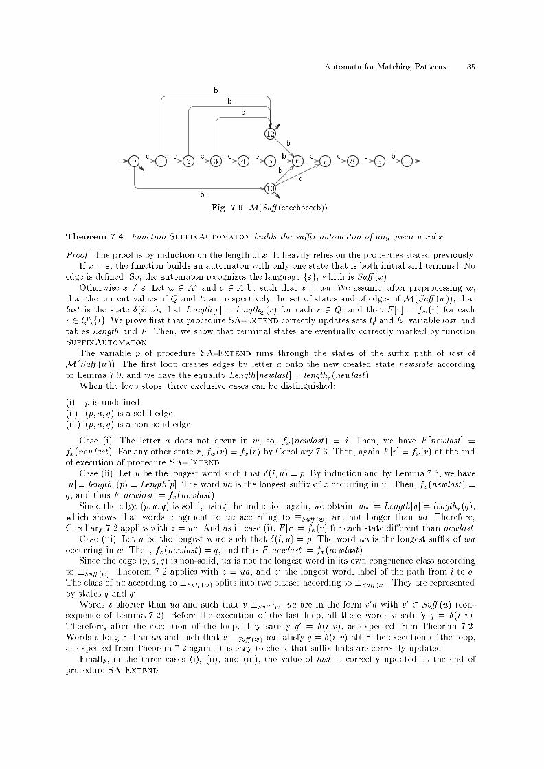
Automata for Matching Patterns 350 1 2 3 4 5 6 7 8 910 1112c c c c b b c c c bb bbb b cbFig. 7.9.M(Su� (ccccbbcccb)).Theorem 7.4. Function SuffixAutomaton builds the su�x automaton of any given word x.Proof. The proof is by induction on the length of x. It heavily relies on the properties stated previously.If x = ", the function builds an automaton with only one state that is both initial and terminal. Noedge is de�ned. So, the automaton recognizes the language f"g, which is Su� (x).Otherwise x 6= ". Let w 2 A� and a 2 A be such that x = wa. We assume, after preprocessing w,that the current values of Q and E are respectively the set of states and of edges of M(Su� (w)), thatlast is the state �(i; w), that Length[r] = lengthw(r) for each r 2 Q, and that F [r] = fw(r) for eachr 2 Qnfig. We prove �rst that procedure SA-Extend correctly updates sets Q and E, variable last, andtables Length and F . Then, we show that terminal states are eventually correctly marked by functionSuffixAutomaton.The variable p of procedure SA-Extend runs through the states of the su�x path of last ofM(Su� (w)). The �rst loop creates edges by letter a onto the new created state newstate accordingto Lemma 7.9, and we have the equality Length [newlast] = lengthx(newlast).When the loop stops, three exclusive cases can be distinguished:(i) p is unde�ned;(ii) (p; a; q) is a solid edge;(iii) (p; a; q) is a non-solid edge.Case (i). The letter a does not occur in w, so, fx(newlast) = i. Then, we have F [newlast] =fx(newlast). For any other state r, fw(r) = fx(r) by Corollary 7.3. Then, again F [r] = fx(r) at the endof execution of procedure SA-Extend.Case (ii). Let u be the longest word such that �(i; u) = p. By induction and by Lemma 7.6, we havejuj = lengthx(p) = Length[p]. The word ua is the longest su�x of x occurring in w. Then, fx(newlast) =q, and thus F [newlast] = fx(newlast).Since the edge (p; a; q) is solid, using the induction again, we obtain juaj = Length [q] = lengthx(q),which shows that words congruent to ua according to �Su� (w) are not longer than ua. Therefore,Corollary 7.2 applies with z = ua. And as in case (i), F [r] = fx(r) for each state di�erent than newlast.Case (iii). Let u be the longest word such that �(i; u) = p. The word ua is the longest su�x of waoccurring in w. Then, fx(newlast) = q, and thus F [newlast] = fx(newlast).Since the edge (p; a; q) is non-solid, ua is not the longest word in its own congruence class accordingto �Su� (w). Theorem 7.2 applies with z = ua, and z0 the longest word, label of the path from i to q.The class of ua according to �Su� (w) splits into two classes according to �Su� (x). They are representedby states q and q0.Words v shorter than ua and such that v �Su� (w) ua are in the form v0a with v0 2 Su� (u) (con-sequence of Lemma 7.2). Before the execution of the last loop, all these words v satisfy q = �(i; v).Therefore, after the execution of the loop, they satisfy q0 = �(i; v), as expected from Theorem 7.2.Words v longer than ua and such that v �Su� (w) ua satisfy q = �(i; v) after the execution of the loop,as expected from Theorem 7.2 again. It is easy to check that su�x links are correctly updated.Finally, in the three cases (i), (ii), and (iii), the value of last is correctly updated at the end ofprocedure SA-Extend.

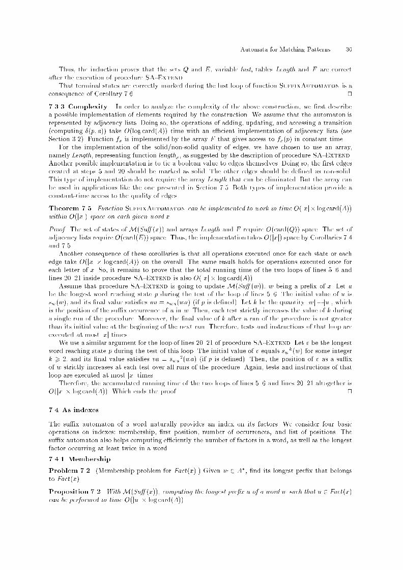
Automata for Matching Patterns 36Thus, the induction proves that the sets Q and E, variable last, tables Length and F are correctafter the execution of procedure SA-Extend.That terminal states are correctly marked during the last loop of function SuffixAutomaton is aconsequence of Corollary 7.6. ut7.3.3 Complexity. In order to analyze the complexity of the above construction, we �rst describea possible implementation of elements required by the construction. We assume that the automaton isrepresented by adjacency lists. Doing so, the operations of adding, updating, and accessing a transition(computing �(p; a)) take O(log card(A)) time with an e�cient implementation of adjacency lists (seeSection 3.2). Function fx is implemented by the array F that gives access to fx(p) in constant time.For the implementation of the solid/non-solid quality of edges, we have chosen to use an array,namely Length, representing function lengthx, as suggested by the description of procedure SA-Extend.Another possible implementation is to tie a boolean value to edges themselves. Doing so, the �rst edgescreated at steps 5 and 20 should be marked as solid. The other edges should be de�ned as non-solid.This type of implementation do not require the array Length that can be eliminated. But the array canbe used in applications like the one presented in Section 7.5. Both types of implementation provide aconstant-time access to the quality of edges.Theorem 7.5. Function SuffixAutomaton can be implemented to work in time O(jxj� log card(A))within O(jxj) space on each given word x.Proof. The set of states ofM(Su� (x)) and arrays Length and F require O(card(Q)) space. The set ofadjacency lists require O(card(E)) space. Thus, the implementation takes O(jxj) space by Corollaries 7.4and 7.5.Another consequence of these corollaries is that all operations executed once for each state or eachedge take O(jxj � log card(A)) on the overall. The same result holds for operations executed once foreach letter of x. So, it remains to prove that the total running time of the two loops of lines 5{6 andlines 20{21 inside procedure SA-Extend is also O(jxj � log card(A)).Assume that procedure SA-Extend is going to update M(Su� (w)), w being a pre�x of x. Let ube the longest word reaching state p during the test of the loop of lines 5{6. The initial value of u issw(w), and its �nal value satis�es ua = swa(wa) (if p is de�ned). Let k be the quantity jwj � juj, whichis the position of the su�x occurrence of u in w. Then, each test strictly increases the value of k duringa single run of the procedure. Moreover, the �nal value of k after a run of the procedure is not greaterthan its initial value at the beginning of the next run. Therefore, tests and instructions of that loop areexecuted at most jxj times.We use a similar argument for the loop of lines 20{21 of procedure SA-Extend. Let v be the longestword reaching state p during the test of this loop. The initial value of v equals swk(w) for some integerk > 2, and its �nal value satis�es va = swa2(wa) (if p is de�ned). Then, the position of v as a su�xof w strictly increases at each test over all runs of the procedure. Again, tests and instructions of thatloop are executed at most jxj times.Therefore, the accumulated running time of the two loops of lines 5{6 and lines 20{21 altogether isO(jxj � log card(A)). Which ends the proof. ut7.4 As indexesThe su�x automaton of a word naturally provides an index on its factors. We consider four basicoperations on indexes: membership, �rst position, number of occurrences, and list of positions. Thesu�x automaton also helps computing e�ciently the number of factors in a word, as well as the longestfactor occurring at least twice in a word.7.4.1 Membership.Problem 7.2. (Membership problem for Fact(x).) Given w 2 A�, �nd its longest pre�x that belongsto Fact(x).Proposition 7.2. With M(Su� (x)), computing the longest pre�x u of a word w such that u 2 Fact(x)can be performed in time O(juj � log card(A)).

Automata for Matching Patterns 37Proof. Just spell the word w in M(Su� (x)) considering the two implementations described in Sec-tion 7.3. Stopping the search on the �rst unde�ned transition gives the longest pre�x u of w for which�(i; u) is de�ned, which means that it is a factor of x. ut7.4.2 First position.Problem 7.3. (First (respectively last) position ofw in x.) Givenw 2 Fact(x), �nd its �rst (respectivelylast) position in x.We assume that w 2 Fact(x). This test (\does w belong to Fact(x)?") can be performed separatelyas in Section 7.4.1, or can be merged with the solution of the present problem.The problem of �nding the �rst position fpx(w) of w in x is equivalent to computing endposx(w)because fpx(w) = endposx(w)� jwj:Moreover, this is also equivalent to computing the maximum length of right contexts of w in x,lcx(w) = maxfjzj j z 2 w�1Fact(x)g;because fpx(w) = jxj � lcx(w)� jwj:Symmetrically, �nding the last position lpx(w) of w in x remains to computing the smallest lengthscx(w) of its right contexts because lpx(w) = jxj � scx(w) � jwj:To be able to answer e�ciently requests on the �rst or last positions of factors of x, we precomputearrays indexed by states of M(Su� (x)) representing functions lcx and scx. We get the next result.Proposition 7.3. The automaton M(Su� (x)) can be preprocessed in time O(jxj) so that the �rst (orlast) position in x of any word w 2 Fact(x) can be computed in time O(jwj� log card(A)) within O(jxj)space.Proof. We consider an array LC de�ned on states of M(Su� (x)) as follows. Let p be a state and u besuch that p = �(i; u); then, we de�ne LC [p] = lcx(u). Note that the value of LC [p] does not depend onthe word u because for an equivalent word v, lcx(u) = lcx(v) (by Lemma 7.2). The array LC satis�esthe induction relation:LC [p] = � 0; if p = lastx,1 + maxfLC [q] j q = �(p; a); a 2 Ag; otherwise.So, the computation of LC can be done during a depth-�rst traversal of the graph ofM(Su� (x)). Sincethe total size of the graph is O(jxj) (Theorem 7.3), this takes time O(jxj).To compute fpx(w), we �rst locate the state p = �(i; w), and then return jxj � jwj � LC [p]. Thistakes the same time as for the membership problem.To �nd the last occurrence of w in x we consider the array SC that represents the function scx.If p = �(i; u), we set SC [p] = scx(u), which is a coherent de�nition. We then use the next relation tocompute the array during a depth-�rst traversal of M(Su� (x)):SC [p] = � 0; if p 2 T ,1 +minfSC [q] j q = �(p; a); a 2 Ag; otherwise.After the preprocessing, we get the same complexity as above. This ends the proof. ut

Automata for Matching Patterns 387.4.3 Occurrence number.Problem 7.4. (Number of occurrences of w in x.) Given w 2 Fact(x), �nd how many times w occursin x.Proposition 7.4. The automaton M(Su� (x)) can be preprocessed in time O(jxj) so that the numberof occurrences in x of any word w 2 Fact(x) can be computed in time O(jwj� log card(A)) within O(jxj)space.Proof. The number of occurrences of w in x iscardfz j z 2 A� and wz 2 Su� (x)g:If �(i; w) = p, this is also cardfz j z 2 A� and �(p; z) 2 Tg:Let NB [p] be this quantity, for any state of M(Su� (x)).The array NB satis�es the recurrence relation:NB [p] = � 1 +Pq=�(p;a);a2A NB [q]; if p 2 T ,Pq=�(p;a);a2A NB [q]; otherwise,which shows that the array NB can be computed in time proportional to the size of the automatonduring a depth-�rst traversal of the graph. This takes O(jxj) time.Afterwards, the problem remains to access NB [p] for p = �(i; w). (If p is unde�ned, w does not occurin x.) Computing p takes the time announced in the statement. utAn argument similar to that of the previous proof gives the computation of the number of factorsoccurring in x, i.e. the size of Fact(x). Indeed, Fact(x) is the particular right context associated withthe initial state of M(Su� (x)). And to compute its size, we evaluate contexts sizes CS [p] of all statesof the automaton using the relation:CS [p] = � 1; if p = lastx,1 +Pq=�(p;a);a2A CS [q]; otherwise.This provides a linear-time computation of card(Fact(x)) = CS [i].7.4.4 List of positions.Problem 7.5. (Positions of w in x.) Given w 2 Fact(x), produce the list of positions of w in x.Proposition 7.5. The automaton M(Su� (x)) can be preprocessed in time O(jxj) so that the list L ofpositions in x of any w 2 Fact(x) can be computed in time O(jwj� log card(A)+card(L)) within O(jxj)space.Proof. We just sketch the proof of the statement. The automaton is preprocessed in order to createshortcuts over states on which exactly one edge is de�ned and that are not terminal states. To doso, we create a graph structure superimposed on the automaton. The nodes of the graph are eitherterminal states or states whose degree is at least two. Arcs of the graph are labeled by the labels of thecorresponding path in the automaton. From a given state, labels of outgoing arcs start with pairwisedistinct letters (because the automaton is deterministic).Once the node q associated with w (or an extension of it) is found in the graph, the list of positionsof w in x is computed by traversing the subgraph rooted at q. Consider the tree of the traversal. Itsinternal nodes have at least two children, and its leaves are associated with distinct positions (somepositions can correspond to internal nodes). Therefore, the number of nodes of the tree is less than2� card(L), which proves that the time of the traversal is O(card(L)). The extra running time is usedto �nd q. ut

Automata for Matching Patterns 397.4.5 Longest repeated factor. There are two dual problems e�ciently solvable with the su�xautomaton of x:{ �nd a longest factor repeated in x;{ �nd a shortest factor occurring only once in x.Problem 7.6. (Longest repeated factor in x.) Produce a longest word u 2 Fact(x) that occurs twicein x.If the table NB used to compute the number of occurrences of a factor is already computed, theproblem is equivalent to �nd the deepest state p in M(Su� (x)) for which NB [p] > 1. The label of thepath from the initial state to p is a solution to the problem. In fact, the problem can be solved withoutany use of the table NB. We just consider the deepest state p which satis�es one of the two conditions:(i) the degree of p is at least two;(ii) p is a terminal state and the degree of p is at least one.Doing so, no preprocessing on M(Su� (x)) is even needed, which gives the following result.Proposition 7.6. With M(Su� (x)), computing a longest repeated factor of x can be performed in timeO(jxj).Given a longest repeated factor u of x, ua is a factor of x for some letter a. It is clear that this wordis a shortest factor occurring once only in x, i.e., this word is a solution to the dual problem. Hence,the proposition also holds for the second problem.7.5 As string-matching automataThe su�x automaton M(Su� (x)) of x can be used to solve the string-matching problem, to locate theoccurrences of x in a word y. The search procedure behaves like the search phase of algorithmMatcher(see Section 2) that processes y in an on-line manner. The existence of failure links in M(Su� (x)) isessential for this application, which gives them their name. The search procedure is a consequence of ageneric procedure, given Figure 7.10, that can be used for other purposes.7.5.1 Ending factors. Procedure EndingFactors of Figure 7.10 computes the longest factor of xending at each position in y, or more exactly the length of this factor. More precisely, we de�ne for eachk 2 f0; : : : ; jyjg the number`k = maxfjwj j w 2 Su� (y1y2 � � �yk) \ Fact(x)g:The procedure EndingFactors performs an on-line computation of the sequence (`k)06k6jyj of lengthsof longest ending factors. The output is given as a word on the alphabet f0; : : : ; jxjg. Function lengthxof Section 7.2 (implemented via table Length) is used to reset properly the current length just after asu�x link has been traversed.The core of procedure EndingFactors is the computation of transitions with the failure table F(implementing the su�x link fx), similarly as in the general method described in Sections 3.4 and 5.4.Theorem 7.6. Procedure EndingFactors computes the lengths of longest ending factors of x in yin time O(jyj � log card(A)). It executes less than 2jyj transitions in M(Su� (x)), and requires O(jxj)space.Proof. See the proof of Theorem 5.3. ut

Automata for Matching Patterns 40EndingFactors((Q; i; T; E);Length; F;y)let � be the transition function of (Q; i; T; E)1 (`; p) (0; i)2 L 03 for letter a from �rst to last letter of y4 loop if �(p; a) 6= nil5 then (`; p) (`+ 1; �(p; a))6 else loop p F [p]7 while p 6= nil and �(p; a) = nil8 if p 6= nil9 then (`; p) (Length[p] + 1; �(p; a))10 else (`; p) (0; i)11 L L � `12 return LFig. 7.10. Computing lengths of factors of a word x ending at all positions in a word y, with (Q; i; T;E) =M(Su� (x)).7.5.2 Optimization of su�x links. Indeed, instead of the su�x link fx, we rather use another link,denoted by f̂x, that optimizes the delay of searches. Its de�nition is based on transitions de�ned onstates of the automaton, and parallels what is done in Section 5.4.The \follow set" of a state q of M(Su� (x)) isFollowx(q) = fa j a 2 A; �(q; a) is de�nedg:Then, f̂x(q) is de�ned by the relation:f̂x(q) = � fx(q); if Followx(fx(q)) * Followx(q),f̂x(fx(q)); otherwise.Note that f̂x(q) can be left unde�ned with this de�nition.A property of Followx sets simpli�es the computation of f̂x. In the su�x automaton we always haveFollowx(q) � Followx(fx(q)). This is because fx(q) corresponds to a su�x v of any word u for whichq = �(i; u). Then, any letter following u in x also follows v (see Lemma 7.1). And this property transfersto follow sets of q and fx(q) respectively. With this remark, the de�nition of the failure function f̂x canbe equivalently stated as:f̂x(q) = � fx(q); if the degrees of q and of fx(q) are di�erent,f̂x(fx(q)); otherwise.Thus, the computation of f̂x has only to consider degrees of states of the automatonM(Su� (x)), andcan be executed in linear time.Proposition 7.7. For procedure EndingFactors using a table, say F̂ , implementing the su�x link f̂xinstead of the table F , the delay is O(card(A)).Proof. This is a consequence of: Followx(q) � Followx(f̂x(q)) � Afor any state q for which f̂x(q) is de�ned. ut7.5.3 Searching for rotations. The knowledge of the sequence of lengths (`k)06k6jyj leads to severalapplications such as searching for x in y, computing lcf (x; y), the maximum length of a factor commonto x and y, or computing the subword distance between two words:d(x; y) = jxj+ jyj � 2� lcf (x; y):The computation of positions of x in y relies on the simple observation:`k = jxj () x occurs at position k � jxj in y:The same remark applies as well to design an e�cient solution to the next problem. A rotation (ora conjugate) of a word u is a word in the form wv, w; v 2 A�, when u = vw.

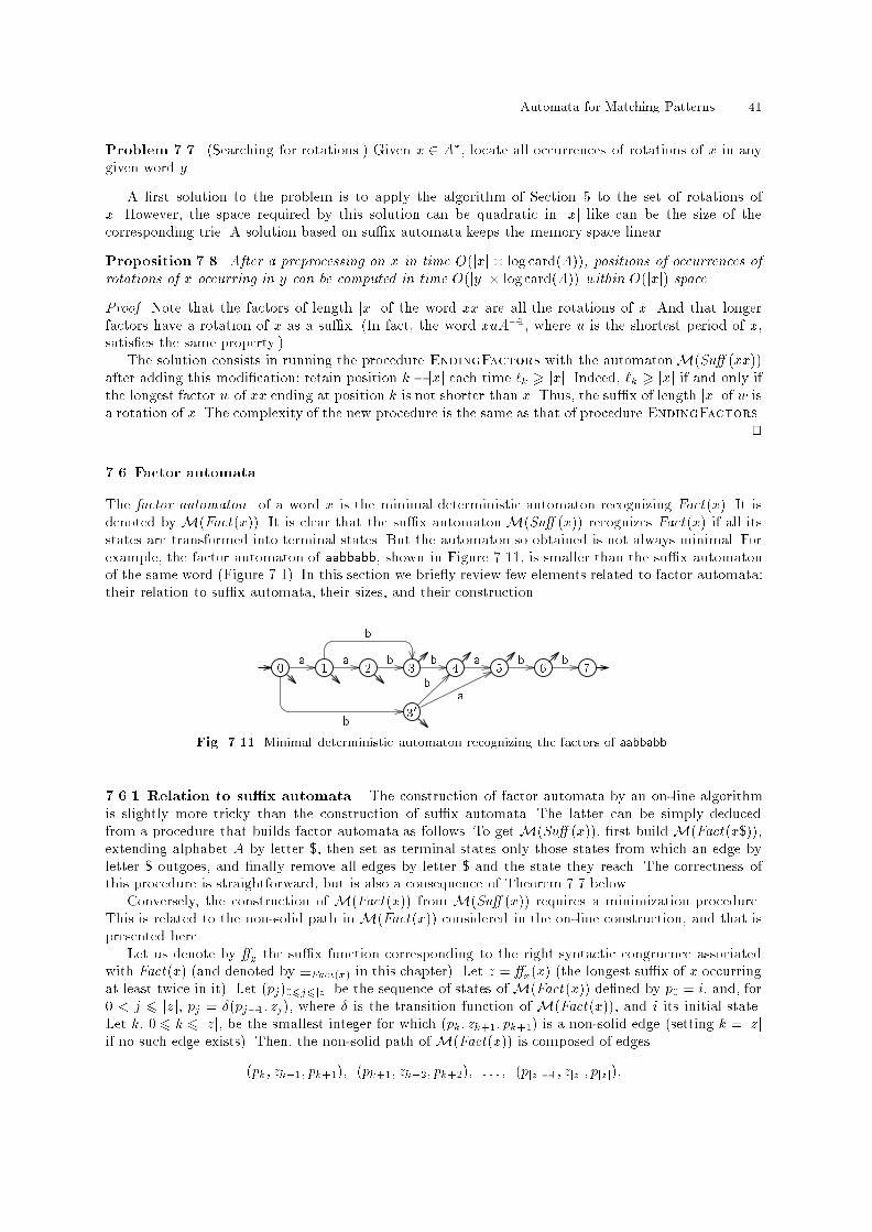
Automata for Matching Patterns 41Problem 7.7. (Searching for rotations.) Given x 2 A�, locate all occurrences of rotations of x in anygiven word y.A �rst solution to the problem is to apply the algorithm of Section 5 to the set of rotations ofx. However, the space required by this solution can be quadratic in jxj like can be the size of thecorresponding trie. A solution based on su�x automata keeps the memory space linear.Proposition 7.8. After a preprocessing on x in time O(jxj � log card(A)), positions of occurrences ofrotations of x occurring in y can be computed in time O(jyj � log card(A)) within O(jxj) space.Proof. Note that the factors of length jxj of the word xx are all the rotations of x. And that longerfactors have a rotation of x as a su�x. (In fact, the word xuA�1, where u is the shortest period of x,satis�es the same property.)The solution consists in running the procedure EndingFactors with the automatonM(Su� (xx))after adding this modi�cation: retain position k � jxj each time `k > jxj. Indeed, `k > jxj if and only ifthe longest factor w of xx ending at position k is not shorter than x. Thus, the su�x of length jxj of w isa rotation of x. The complexity of the new procedure is the same as that of procedure EndingFactors.ut7.6 Factor automataThe factor automaton of a word x is the minimal deterministic automaton recognizing Fact(x). It isdenoted by M(Fact(x)). It is clear that the su�x automatonM(Su� (x)) recognizes Fact(x) if all itsstates are transformed into terminal states. But the automaton so obtained is not always minimal. Forexample, the factor automaton of aabbabb, shown in Figure 7.11, is smaller than the su�x automatonof the same word (Figure 7.1). In this section we brie y review few elements related to factor automata:their relation to su�x automata, their sizes, and their construction.0 1 2 3 4 5 6 730a a b b a b bb b abFig. 7.11. Minimal deterministic automaton recognizing the factors of aabbabb.7.6.1 Relation to su�x automata. The construction of factor automata by an on-line algorithmis slightly more tricky than the construction of su�x automata. The latter can be simply deducedfrom a procedure that builds factor automata as follows. To get M(Su� (x)), �rst build M(Fact(x$)),extending alphabet A by letter $, then set as terminal states only those states from which an edge byletter $ outgoes, and �nally remove all edges by letter $ and the state they reach. The correctness ofthis procedure is straightforward, but is also a consequence of Theorem 7.7 below.Conversely, the construction of M(Fact(x)) from M(Su� (x)) requires a minimization procedure.This is related to the non-solid path in M(Fact(x)) considered in the on-line construction, and that ispresented here.Let us denote by �x the su�x function corresponding to the right syntactic congruence associatedwith Fact(x) (and denoted by �Fact(x) in this chapter). Let z = �x(x) (the longest su�x of x occurringat least twice in it). Let (pj)06j6jzj be the sequence of states ofM(Fact(x)) de�ned by p0 = i, and, for0 < j 6 jzj, pj = �(pj�1; zj), where � is the transition function of M(Fact(x)), and i its initial state.Let k, 0 6 k 6 jzj, be the smallest integer for which (pk; zk+1; pk+1) is a non-solid edge (setting k = jzjif no such edge exists). Then, the non-solid path of M(Fact(x)) is composed of edges(pk; zk+1; pk+1); (pk+1; zk+2; pk+2); : : : ; (pjzj�1; zjzj; pjzj):

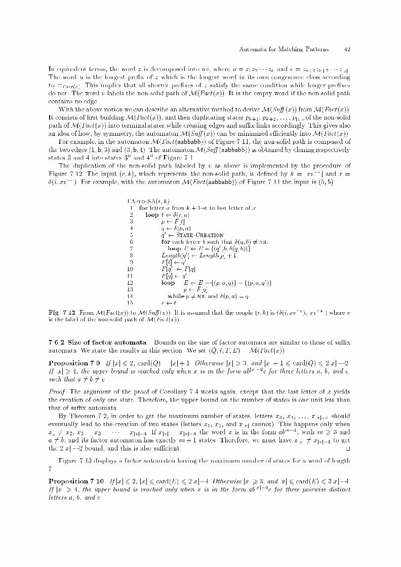
Automata for Matching Patterns 42In equivalent terms, the word z is decomposed into uv, where u = z1z2 � � � zk and v = zk+1zk+2 � � �zjzj.The word u is the longest pre�x of z which is the longest word in its own congruence class accordingto �Fact(x). This implies that all shorter pre�xes of z satisfy the same condition while longer pre�xesdo not. The word v labels the non-solid path ofM(Fact(x)). It is the empty word if the non-solid pathcontains no edge.With the above notion we can describe an alternative method to deriveM(Su� (x)) fromM(Fact(x)).It consists of �rst buildingM(Fact(x)), and then duplicating states pk+1, pk+2, : : : , pjzj, of the non-solidpath ofM(Fact(x)) into terminal states while creating edges and su�x links accordingly. This gives alsoan idea of how, by symmetry, the automatonM(Su� (x)) can be minimized e�ciently intoM(Fact(x)).For example, in the automatonM(Fact(aabbabb)) of Figure 7.11, the non-solid path is composed ofthe two edges (1; b; 3) and (3; b; 4). The automatonM(Su� (aabbabb)) is obtained by cloning respectivelystates 3 and 4 into states 300 and 400 of Figure 7.1.The duplication of the non-solid path labeled by v as above is implemented by the procedure ofFigure 7.12. The input (r; k), which represents the non-solid path, is de�ned by k = jxv�1j and r =�(i; xv�1). For example, with the automatonM(Fact(aabbabb)) of Figure 7.11 the input is (5; 5).FA-to-SA(r; k)1 for letter a from k + 1-st to last letter of x2 loop t �(r; a)3 p F [t]4 q �(p; a)5 q0 State-Creation6 for each letter b such that �(q; b) 6= nil7 loop E E + f(q0; b; �(q; b))g8 Length[q0] Length[p] + 19 F [t] q010 F [q0] F [q]11 F [q] q012 loop E E � f(p; a; q)g+ f(p; a; q0)g13 p F [q]14 while p 6= nil and �(p; a) = q15 r tFig. 7.12. FromM(Fact(x)) toM(Su� (x)). It is assumed that the couple (r; k) is (�(i; xv�1); jxv�1j) where vis the label of the non-solid path ofM(Fact(x)).7.6.2 Size of factor automata. Bounds on the size of factor automata are similar to those of su�xautomata. We state the results in this section. We set (Q; i; T;E) =M(Fact(x)).Proposition 7.9. If jxj 6 2, card(Q) = jxj+ 1. Otherwise jxj > 3, and jxj+ 1 6 card(Q) 6 2jxj � 2.If jxj > 4, the upper bound is reached only when x is in the form abjxj�2c for three letters a, b, and c,such that a 6= b 6= c.Proof. The argument of the proof of Corollary 7.4 works again, except that the last letter of x yieldsthe creation of only one state. Therefore, the upper bound on the number of states is one unit less thanthat of su�x automata.By Theorem 7.2, in order to get the maximum number of states, letters x3, x4, : : : , xjxj�1 shouldeventually lead to the creation of two states (letters x1, x2, and xjxj cannot). This happens only whenx1 6= x2, x2 = x3 = � � � = xjxj�1. If xjxj = xjxj�1 the word x is in the form abm�1, with m > 3 anda 6= b, and its factor automaton has exactly m+ 1 states. Therefore, we must have xjxj 6= xjxj�1 to getthe 2jxj � 2 bound, and this is also su�cient. utFigure 7.13 displays a factor automaton having the maximum number of states for a word of length7.Proposition 7.10. If jxj 6 2, jxj 6 card(E) 6 2jxj�1. Otherwise jxj > 3, and jxj 6 card(E) 6 3jxj�4.If jxj > 4, the upper bound is reached only when x is in the form abjxj�2c for three pairwise distinctletters a, b, and c.

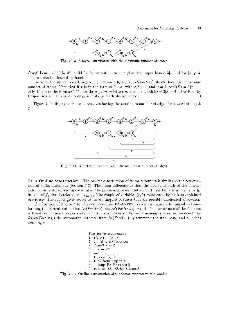
Automata for Matching Patterns 430 1 2 3 4 5 6 78 9 10 11a b b b b b ab b b b b aFig. 7.13. A factor automaton with the maximum number of states.Proof. Lemma 7.10 is still valid for factor automata, and gives the upper bound 3jxj � 4 for jxj > 3.The rest can be checked by hand.To reach the upper bound, regarding Lemma 7.10 again, M(Fact(x)) should have the maximumnumber of states. Note that if x is in the form abjxj�2a, with a; b 2 A and a 6= b, card(E) = 2jxj � 1only. If x is in the form abjxj�2c for three pairwise letters a, b, and c, card(E) = 3jxj � 4. Therefore, byProposition 7.9, this is the only possibility to reach the upper bound. utFigure 7.14 displays a factor automaton having the maximum number of edges for a word of length7. 0 1 2 3 4 5 6 78 9 10 11a b b b b b cb b b b b cccccFig. 7.14. A factor automaton with the maximum number of edges.7.6.3 On-line construction. The on-line construction of factor automata is similar to the construc-tion of su�x automata (Section 7.3). The main di�erence is that the non-solid path of the currentautomaton is stored and updated after the processing of each letter, and that table F implements �xinstead of fx that is related to �Su� (x). The couple of variables (r; k) represents the path as explainedpreviously. The couple gives access to the waiting list of states that are possibly duplicated afterwards.The function of Figure 7.15 relies on procedure FA-Extend (given in Figure 7.16) aimed at trans-forming the current automatonM(Fact(w)) intoM(Fact(wa)), a 2 A. The correctness of the functionis based on a crucial property stated in the next theorem. For each nonempty word w, we denote byR(M(Fact(w))) the automaton obtained from M(Fact(w)) by removing the state lastw and all edgesreaching it. FactorAutomaton(x)1 (Q;E) (?;?)2 i State-Creation3 Length[i] 04 F [i] nil5 last i6 (r; k) (i; 0)7 for ` from 1 up to x8 loop FA-Extend(`)9 return (Q; i;Q;E);Length; FFig. 7.15. On-line construction of the factor automaton of a word x.

Automata for Matching Patterns 44Theorem 7.7. Let w 2 A�, z the longest su�x of w that occurs at least twice in it, and a 2 A. Ifza 62 Fact(w), then, disregarding terminal states,R(M(Fact(wa))) =M(Su� (w)):Before proving the theorem, we prove the following lemma.Lemma 7.11. Let w 2 A�, z the longest su�x of w that occurs twice in it, and a 2 A. If za 62 Fact(w),then, for each s 2 A�, we have s �Fact(wa) z =) s 2 Su� (z):Proof. The condition on z implies that (za)�1Fact(wa) = f"g. Then, we have (sa)�1Fact(wa) = f"g,which implies that s is a su�x of w. Since z occurs twice in w, this is also the case for s (because someword ta, with t 6= ", belongs to z�1Fact(wa) = s�1Fact(wa)). Therefore, by the de�nition of z, s is asu�x of z. utProof of Theorem 7.7. We prove that, for any words u; v 2 Fact(w),u �Fact(wa) v () u �Su� (w) v;which is a re-statement of the conclusion of the theorem.Assume �rst u �Fact(wa) v. After Lemma 7.2 we can consider, for example, that u 2 Su� (v). Then,v�1Su� (w) � u�1Su� (w), and to prove u �Su� (w) v it remains to show u�1Su� (w) � v�1Su� (w).Let t 2 u�1Su� (w). We show that t 2 v�1Su� (w). Since ut 2 Su� (w), we have uta 2 Su� (wa) �Fact(wa), and using the hypothesis, namely u �Fact(wa) v, we get that vta 2 Fact(wa). If ut occurs onlyonce in w, (ut)�1Fact(w) = f"g. Therefore, (vt)�1Fact(w) = f"g because �Fact(wa) is a congruence,which proves that vt 2 Su� (w), i.e. t 2 v�1Su� (w). If ut occurs at least twice in w, by de�nition of z,ut is a su�x of z. So, z = z0ut for some pre�x z0 of z. Then, z0vt �Fact(wa) z, which implies that vt is asu�x of z and consequently of w by Lemma 7.11. Hence again, t 2 v�1Su� (w). This ends the �rst partof the statement.Conversely, let us consider that u �Su� (w) v, and prove u �Fact(wa) v. Without loss of generality, weassume u 2 Su� (v), so it remains to prove u�1Fact(wa) � v�1Fact(wa).Let t 2 u�1Fact(wa). If t = ", t 2 v�1Fact(wa) because v 2 Fact(w). We then assume that t isa nonempty word. If ut 2 Fact(w), for some t0 2 A�, utt0 2 Su� (w), that is tt0 2 u�1Su� (w). Thehypothesis u �Su� (w) v implies tt0 2 v�1Su� (w), and consequently t 2 v�1Fact(wa). If vt 62 Fact(w), t isa su�x of wa. It can be written t0a for some su�x t0 of w. So, t0 2 u�1Su� (w), and then t0 2 v�1Su� (w)which shows that vt0 is a su�x of w. Therefore, t 2 v�1Fact(wa). This ends both the second part of thestatement and the whole proof. utDuring the construction ofM(Fact(x)), the following property is invariant: let M(Fact(w)) be thecurrent automaton and z be as in Theorem 7.7, then �(i; z) = F [last]. Consequently, the condition onz that appears in Theorem 7.7 translates into the test \�(F [last]; a) 6= nil". If its value is true, theautomaton and the su�x z extend, and the procedure FA-Extend updates the pair (r; k) if necessaryin a natural way. Otherwise, Theorem 7.7 applies, which leads to �rst transform M(Fact(w)) intoM(Su� (w)). After that, the automaton is extended by the letter a. In this situation, the new non-solidpath is composed of at most one edge, as a consequence of Lemma 7.6 (see also the proof of Theorem 7.7).Finally, we state the complexity of function FactorAutomaton: the construction of factor au-tomata by this function takes linear time on a �xed alphabet.Theorem 7.8. Function FactorAutomaton can be implemented to work on the input word x in timeO(jxj � log card(A)) within O(jxj) space.Proof. If, for a moment, we do not consider the calls to procedure FA-to-SA, it is rather simpleto see that there is a linear number of instructions executed to built M(Fact(x)). Implementing theautomaton with adjacency lists, the cost of computing a transition is O(log card(A)). Which gives theO(jxj � log card(A)) time for the considered instructions.

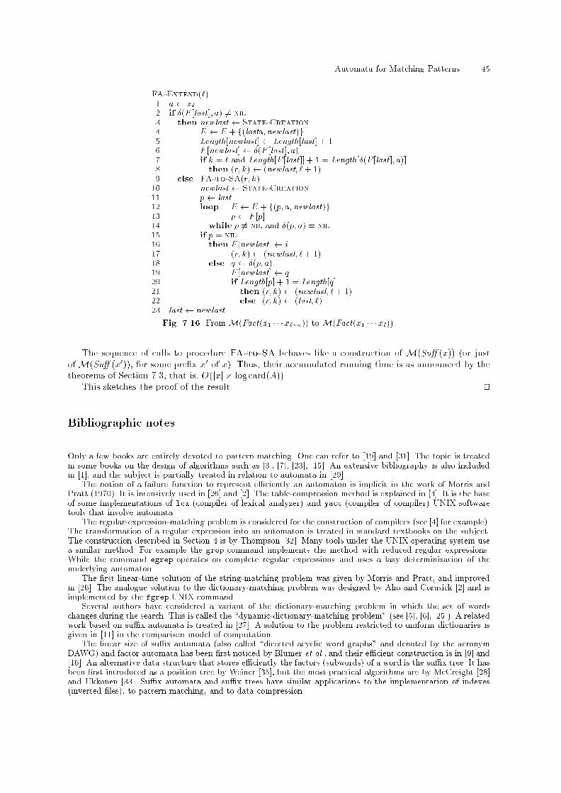
Automata for Matching Patterns 45FA-Extend(`)1 a x`2 if �(F [last]; a) 6= nil3 then newlast State-Creation4 E E + f(lasta;newlast)g5 Length[newlast] Length[last] + 16 F [newlast] �(F [last]; a)7 if k = ` and Length[F [last]] + 1 = Length[�(F [last]; a)]8 then (r; k) (newlast; `+ 1)9 else FA-to-SA(r; k)10 newlast State-Creation11 p last12 loop E E + f(p; a; newlast)g13 p F [p]14 while p 6= nil and �(p; a) = nil15 if p = nil16 then F [newlast] i17 (r; k) (newlast; `+ 1)18 else q �(p; a)19 F [newlast] q20 if Length[p] + 1 = Length[q]21 then (r; k) (newlast; `+ 1)22 else (r; k) (last; `)23 last newlastFig. 7.16. FromM(Fact(x1 � � �x`�1)) toM(Fact(x1 � � �x`)).The sequence of calls to procedure FA-to-SA behaves like a construction of M(Su� (x)) (or justof M(Su� (x0)), for some pre�x x0 of x). Thus, their accumulated running time is as announced by thetheorems of Section 7.3, that is, O(jxj � log card(A)).This sketches the proof of the result. utBibliographic notesOnly a few books are entirely devoted to pattern matching. One can refer to [19] and [31]. The topic is treatedin some books on the design of algorithms such as [3], [7], [23], [15]. An extensive bibliography is also includedin [1], and the subject is partially treated in relation to automata in [29].The notion of a failure function to represent e�ciently an automaton is implicit in the work of Morris andPratt (1970). It is intensively used in [26] and [2]. The table-compression method is explained in [4]. It is the baseof some implementations of lex (compiler of lexical analyzer) and yacc (compiler of compiler) UNIX softwaretools that involve automata.The regular-expression-matching problem is considered for the construction of compilers (see [4] for example).The transformation of a regular expression into an automaton is treated in standard textbooks on the subject.The construction described in Section 4 is by Thompson [32]. Many tools under the UNIX operating system usea similar method. For example the grep command implements the method with reduced regular expressions.While the command egrep operates on complete regular expressions and uses a lazy determinization of theunderlying automaton.The �rst linear-time solution of the string-matching problem was given by Morris and Pratt, and improvedin [26]. The analogue solution to the dictionary-matching problem was designed by Aho and Corasick [2] and isimplemented by the fgrep UNIX command.Several authors have considered a variant of the dictionary-matching problem in which the set of wordschanges during the search. This is called the \dynamic-dictionary-matching problem" (see [5], [6], [25]). A relatedwork based on su�x automata is treated in [27]. A solution to the problem restricted to uniform dictionaries isgiven in [11] in the comparison model of computation.The linear size of su�x automata (also called \directed acyclic word graphs" and denoted by the acronymDAWG) and factor automata has been �rst noticed by Blumer et al., and their e�cient construction is in [9] and[16]. An alternative data structure that stores e�ciently the factors (subwords) of a word is the su�x tree. It hasbeen �rst introduced as a position tree by Weiner [35], but the most practical algorithms are by McCreight [28]and Ukkonen [33]. Su�x automata and su�x trees have similar applications to the implementation of indexes(inverted �les), to pattern matching, and to data compression.

Automata for Matching Patterns 46The solution of the string-matching problem presented in Section 6 is adapted from an original algorithmof Simon [30]. It has been analyzed and improved by Hancart [24]. These algorithms as well as algorithms in[26] solve the string-pre�x-matching problem which is the computation of ending pre�xes at each position onthe searched word. Breslauer et al. [12] gave lower bounds to this problem that meet the upper bounds ofTheorem 6.7. Galil showed in [20] how to transform the algorithms of Knuth, Morris and Pratt, so that thesearch phase works in real time (independently of the alphabet). This applies as well to the algorithm of Simon.There are many other solutions to the string-matching problem if we relax the condition that the bu�eron the searched word is reduced to only one letter. The most practically e�cient solutions are based on thealgorithm of Boyer and Moore [10]. With the use of automata, it has been extended to the dictionary-matchingproblem by Commentz-Walter [14] (see also [1]) and by Crochemore et al. (see [19]). The set of con�gurationspossibly met during the search phase of a variant of the algorithm of Boyer and Moore in which all informationis retained leads to what is called the \Boyer-Moore automaton". It is still unknown if the number of states ofthe automaton is polynomial as conjectured by Knuth (see [26, 13, 8]). Theorem 6.3 is by Galil and Seiferas [21].Like their solution, several other proofs (in [18, 17, 22]) of the same result are based on combinatorial propertiesof words (see Chapter \Combinatorics of words").Other kinds of patterns are considered in the approximate string-matching problem (see [19] for referenceson the subject). The �rst kind arises when mismatches are allowed between a given word and factors of thesearched word (base of the Hamming distance). A second kind of patterns arises when approximate patterns arede�ned by transformation rules (substitution, insertion, and deletion) that yield the edit distance (see Chapter\String editing and DNA"). This notion is widely used for matching patterns in DNA sequences (see [34]).References1. A. V. Aho. Algorithms for �nding patterns in strings. In J. van Leeuwen, editor, Handbook of TheoreticalComputer Science, volume A, chapter 5, pages 255{300. Elsevier, Amsterdam, 1990.2. A. V. Aho and M. J. Corasick. E�cient string matching: an aid to bibliographic search. Communications ofthe ACM, 18:333{340, 1975.3. A. V. Aho, J. E. Hopcroft, and J. D. Ullman. The design and analysis of computer algorithms. Addison-Wesley, Reading, MA, 1974.4. A. V. Aho, R. Sethi, and J. D. Ullman. Compilers { Principles, techniques and tools. Addison-Wesley,Reading, MA, 1986.5. A. Amir and M. Farach. Adaptative dictionary matching. In Proceedings of the 32th IEEE Annual Symposiumon Foundations of Computer Science, pages 760{766. IEEE Computer Society Press, 1991.6. A. Amir, M. Farach, Z. Galil, R. Giancarlo, and K. Park. Fully dynamic dictionary matching. Journal ofComputer and System Sciences, 49:208{222, 1994.7. S. Baase. Computer algorithms { Introduction to design and analysis. Addison-Wesley, Reading, MA, 1988.8. R. A. Baeza-Yates, C. Cho�rut, and G. H. Gonnet. On Boyer-Moore automata. Algorithmica, 12:268{292,1994.9. A. Blumer, J. Blumer, A. Ehrenfeucht, D. Haussler, M. T. Chen, and J. Seiferas. The smallest automatonrecognizing the subwords of a text. Theoretical Computer Science, 40:31{55, 1985.10. R. S. Boyer and J. S. Moore. A fast string searching algorithm. Communications of the ACM, 20:762{772,1977.11. D. Breslauer. Dictionary-matching on unbounded alphabets: uniform length dictionaries. Journal of Algo-rithms, 18:278{295, 1995.12. D. Breslauer, L. Colussi, and L. Toniolo. Tight comparison bounds for the string pre�x-matching problem.Information Processing Letters, 47:51{57, 1993.13. V. Bruy�ere. Automates de Boyer-Moore. Th�ese annexe, Universit�e de Mons-Hainaut, Belgique, 1991.14. B. Commentz-Walter. A string matching algorithm fast on the average. In Proceedings of the 6th Interna-tional Conference on Automata, Languages and Programmation, Lecture Notes in Computer Science, pages118{132. Springer-Verlag, Berlin, 1979.15. T. H. Cormen, C. E. Leiserson, and R. L. Rivest. Introduction to algorithms. MIT Press, 1990.16. M. Crochemore. Transducers and repetitions. Theoretical Computer Science, 45:63{86, 1986.17. M. Crochemore. String-matching on ordered alphabets. Theoretical Computer Science, 92:33{47, 1992.18. M. Crochemore and D. Perrin. Two-way string-matching. Journal of the ACM, 38:651{675, 1991.19. M. Crochemore and W. Rytter. Text algorithms. Oxford University Press, 1994.20. Z. Galil. String matching in real time. Journal of the ACM, 28:134{149, 1981.21. Z. Galil and J. Seiferas. Time-space optimal string matching. Journal of Computer and System Sciences,26:280{294, 1983.22. L. G�asieniec, W. Plandowski, and W. Rytter. The zooming method: a recursive approach to time-spacee�cient string-matching. Theoretical Computer Science, 147:19{30, 1995.

Automata for Matching Patterns 4723. G. H. Gonnet and R. A. Baeza-Yates. Handbook of algorithms and data structures. Addison-Wesley, Reading,MA, 1991.24. C. Hancart. On Simon's string searching algorithm. Information Processing Letters, 47:95{99, 1993.25. R. M. Idury and A. A. Sch�a�er. Dynamic dictionary matching with failure function. Theoretical ComputerScience, 131:295{310, 1994.26. D. E. Knuth, J. H. Morris, Jr, and V. R. Pratt. Fast pattern matching in strings. SIAM Journal onComputing, 6:323{350, 1977.27. G. Kucherov and M. Rusinowitch. Matching a set of strings with variable length don't cares. In Proceedingsof the 6th Annual Symposium on Combinatorial Pattern Matching, number 937 in Lecture Notes in ComputerScience, pages 230{247. Springer-Verlag, Berlin, 1995.28. E. M. McCreight. A space-economical su�x tree construction algorithm. Journal of Algorithms, 23:262{272,1976.29. D. Perrin. Finite automata. In J. van Leeuwen, editor, Handbook of Theoretical Computer Science, volume B,chapter 1, pages 1{57. Elsevier, Amsterdam, 1990.30. I. Simon. String matching algorithms and automata. In Results and Trends in Theoretical Computer Science,number 814 in Lecture Notes in Computer Science, pages 386{395. Springer-Verlag, Berlin, 1994.31. G. A. Stephen. String searching algorithms. World Scienti�c Press, 1994.32. K. Thompson. Regular expression search algorithm. Communications of the ACM, 11:419{422, 1968.33. E. Ukkonen. Constructing su�x trees on-line in linear time. In J. van Leeuwen, editor, Proceedings of theIFIP 12th World Computer Congress, pages 484{492, Madrid, 1992. North-Holland.34. M. S. Waterman. Introduction to computational biology. Chapman and Hall, 1995.35. P. Weiner. Linear pattern matching algorithm. In Proceedings of the 14th Annual IEEE Symposium onSwitching and Automata Theory, pages 1{11, 1973.

IndexAlgorithm 6Automaton 2, 4, 10, 13, 15, 19, 21, 26, 41{ determinization 2, 12{ implementation 6Border of a word 19Conjugate of a word 40Delay 6Dictionary 2, 12Factor automaton 41Failure function 7, 14, 32Index 2, 27, 36Occurrence of a pattern 5Pattern matching 2, 5Periodicity lemma 19Regular expression 2, 3, 8Repeated factor 39Rotation of a word 40String matching 3, 18Subword distance 40Su�x automaton 2, 26Syntactic congruence 3, 28, 41Trie 14, 27

48