Automated Analysis of Simulation Output Data and

the AutoSimOA Project

Stewart Robinson and Katy Hoad and Ruth Davies

Warwick Business School

Simulation Group Seminar, 5 May 2006

Outline

The problem

An automated output Analyser:• Warm-up analysis• Replications analysis• Run-length analysis: batch means method

Example (demonstration)

Discussion

The AutoSimOA Project

The Problem

Prevalence of simulation software: ‘easy-to-develop’ models and use by non-experts.

Simulation software generally have very limited facilities for directing/advising on simulation experiments.

Main exception is directing scenario selection through ‘optimisers’.

With a lack of the necessary skills and support, it is highly likely that simulation users are using their models poorly.

The Problem

Despite continued theoretical developments in simulation output analysis, little is being put into practical use.

There are 3 factors that seem to inhibit the adoption of output analysis methods:

• Limited testing of methods• Requirement for detailed statistical knowledge• Methods generally not implemented in simulation

software (AutoMod/AutoStat is an exception)

A solution would be to provide an automated output ‘Analyser’.

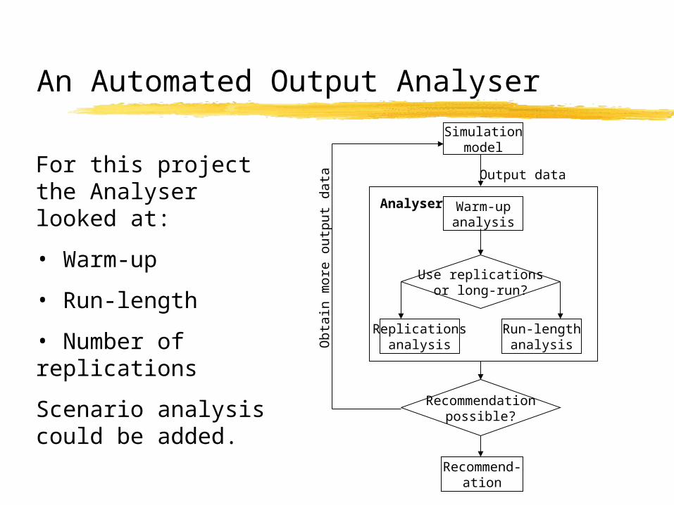
An Automated Output Analyser

Simulationmodel

Warm-upanalysis

Run-lengthanalysis

Replicationsanalysis

Use replicationsor long-run?

Recommendationpossible?

Recommend-ation

Output data

Analyser

Obt

ain

mor

e ou

tput

dat

a

For this project the Analyser looked at:

• Warm-up

• Run-length

• Number of replications

Scenario analysis could be added.

An Automated Output Analyser

A prototype Analyser has been developed in Microsoft Excel.

At present it links to the SIMUL8 software, but it could be used with any software that can be controlled from Excel VBA.

Warm-up Analysis

The Analyser uses 3 procedures from which the user can select the desired warm-up period: MSER-5, Batch Means Bias Detection, Welch’s Method.

The 3 procedures were chosen on the basis of:• Accuracy• Reliability• Generality• Ease of implementation (in Excel)• Requires minimum user intervention• Varied (e.g. not all graphical procedures)

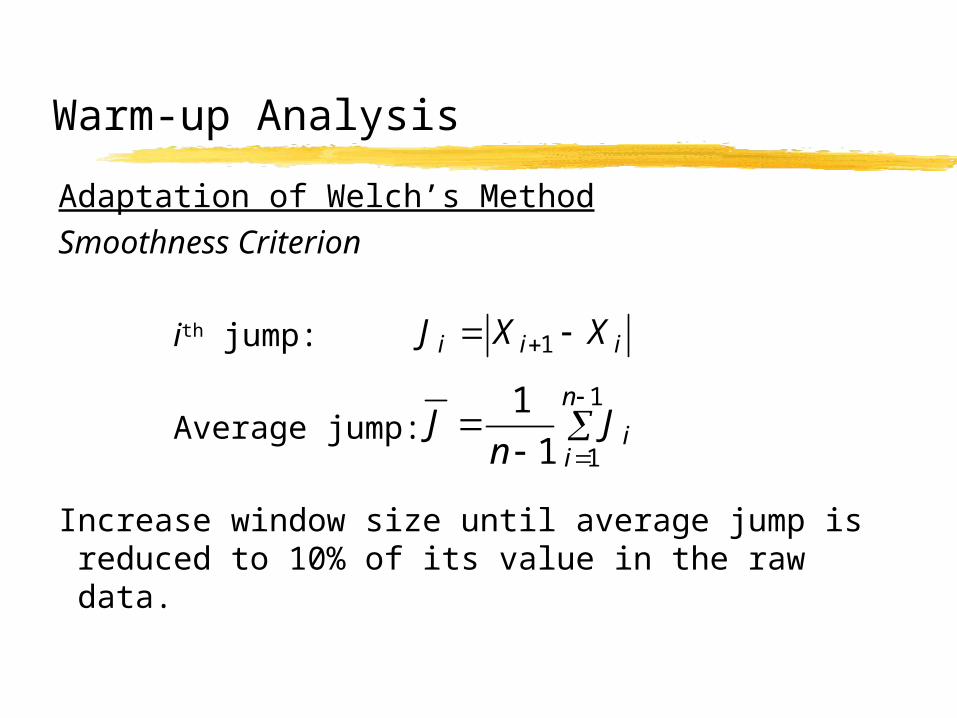
Warm-up Analysis

Adaptation of Welch’s Method

Smoothness Criterion

ith jump:

Average jump:

Increase window size until average jump is reduced to 10% of its value in the raw data.

iii XXJ 1

1

11

1 n

iiJn

J

Warm-up Analysis

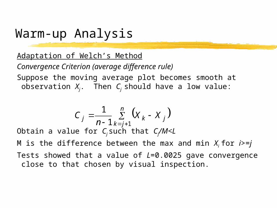
Adaptation of Welch’s Method

Convergence Criterion (average difference rule)

Suppose the moving average plot becomes smooth at observation Xj. Then Cj should have a low value:

Obtain a value for Cj such that Cj/M<L

M is the difference between the max and min Xi for i>=j

Tests showed that a value of L=0.0025 gave convergence close to that chosen by visual inspection.

n

jkjkj XX

nC

11

1

Replications Analysis

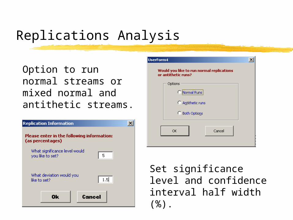
Option to run normal streams or mixed normal and antithetic streams.

Set significance level and confidence interval half width (%).

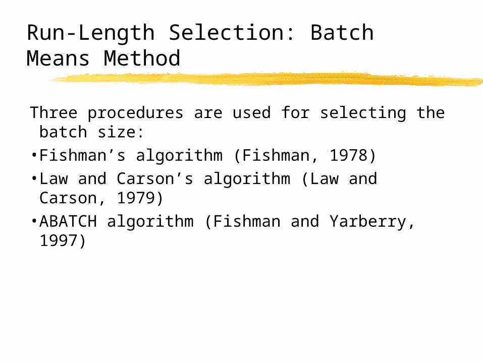
Run-Length Selection: Batch Means Method

Three procedures are used for selecting the batch size:• Fishman’s algorithm (Fishman, 1978)• Law and Carson’s algorithm (Law and Carson, 1979)• ABATCH algorithm (Fishman and Yarberry, 1997)

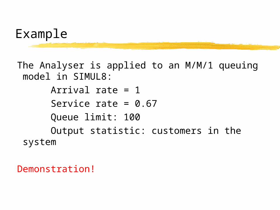
Example

The Analyser is applied to an M/M/1 queuing model in SIMUL8:

Arrival rate = 1

Service rate = 0.67

Queue limit: 100

Output statistic: customers in the system

Demonstration!

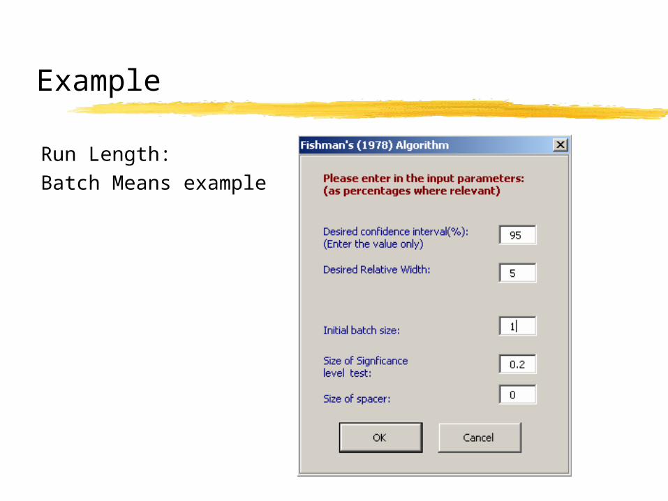
Example

Run Length:

Batch Means example

Example

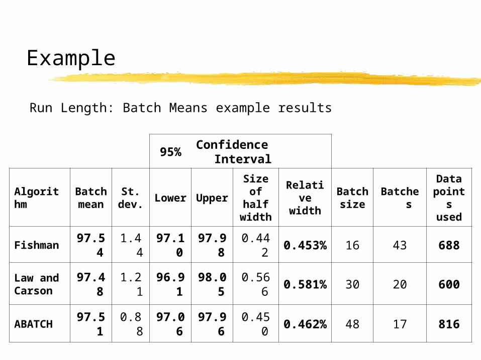
Run Length: Batch Means example results

95% Confidence Interval  

AlgorithmBatch mean

St. dev.

Lower UpperSize of

half width

Relative width

Batch size

BatchesData

points used

Fishman 97.54 1.44 97.10 97.98 0.442 0.453% 16 43 688

Law and Carson 97.48 1.21 96.91 98.05 0.566 0.581% 30 20 600

ABATCH 97.51 0.88 97.06 97.96 0.450 0.462% 48 17 816

Discussion

It is possible to link an Automated Analyser in Excel to a simulation software tool.

At present this is just a proof of concept.

Key issues to address:• More thorough testing of output analysis methods for their

accuracy and their generality.• Adaptation of methods to sequential procedures and to

minimise the need for user intervention.

A 3 year, EPSRC funded project in collaboration with SIMUL8 Corporation.

The AutoSimOA Project

Objectives

• To determine the most appropriate methods for automating simulation output analysis

• To determine the effectiveness of the analysis methods• To revise the methods where necessary in order to

improve their effectiveness and capacity for automation• To propose a procedure for automated output analysis of

warm-up, replications and run-length

Only looking at analysis of a single scenario

The AutoSimOA Project

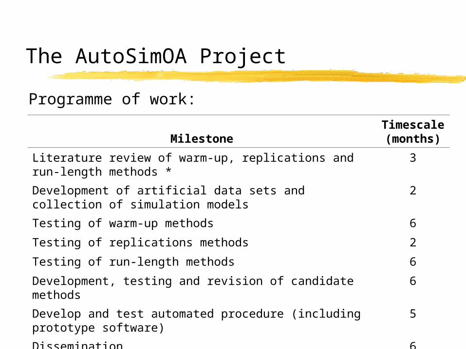
MilestoneTimescale (months)

Literature review of warm-up, replications and run-length methods * 3

Development of artificial data sets and collection of simulation models 2

Testing of warm-up methods 6

Testing of replications methods 2

Testing of run-length methods 6

Development, testing and revision of candidate methods 6

Develop and test automated procedure (including prototype software) 5

Dissemination 6

Total 36

Programme of work:

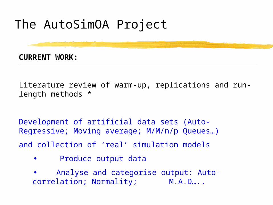
The AutoSimOA Project

CURRENT WORK:

Literature review of warm-up, replications and run-length methods *

Development of artificial data sets (Auto-Regressive; Moving average; M/M/n/p Queues…)

and collection of ‘real’ simulation models

• Produce output data

• Analyse and categorise output: Auto-correlation; Normality; M.A.D…..

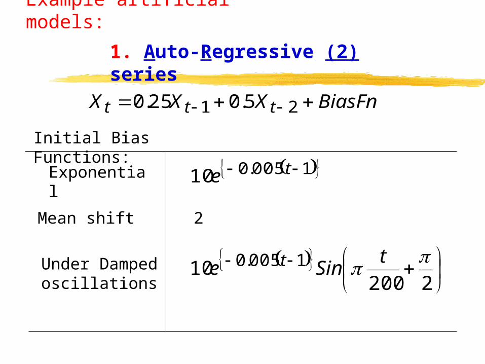
Example artificial models:

1. Auto-Regressive (2) series

BiasFnXXX ttt 21 5.025.0

1005.010 te

220010 1005.0 t

Sine t

Exponential

Under Damped oscillations

Mean shift 2

Initial Bias Functions:

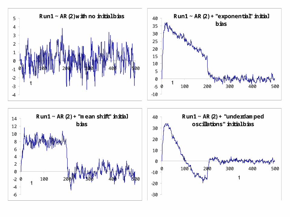
Run1 ~ AR(2) + "underdamped oscillations" initial bias

-30

-20

-10

0

10

20

30

40

0 100 200 300 400 500

t

Run1 ~ AR(2) + "mean shift" initial bias

-6

-4

-2

0

2

4

6

8

10

12

14

0 100 200 300 400 500t

Run1 ~ AR(2) + "exponential" initial bias

-10

-5

0

5

10

15

20

25

30

35

40

0 100 200 300 400 500t

Run1 ~ AR(2) with no initial bias

-4

-3

-2

-1

0

1

2

3

4

5

0 100 200 300 400 500

t

mean 1.8

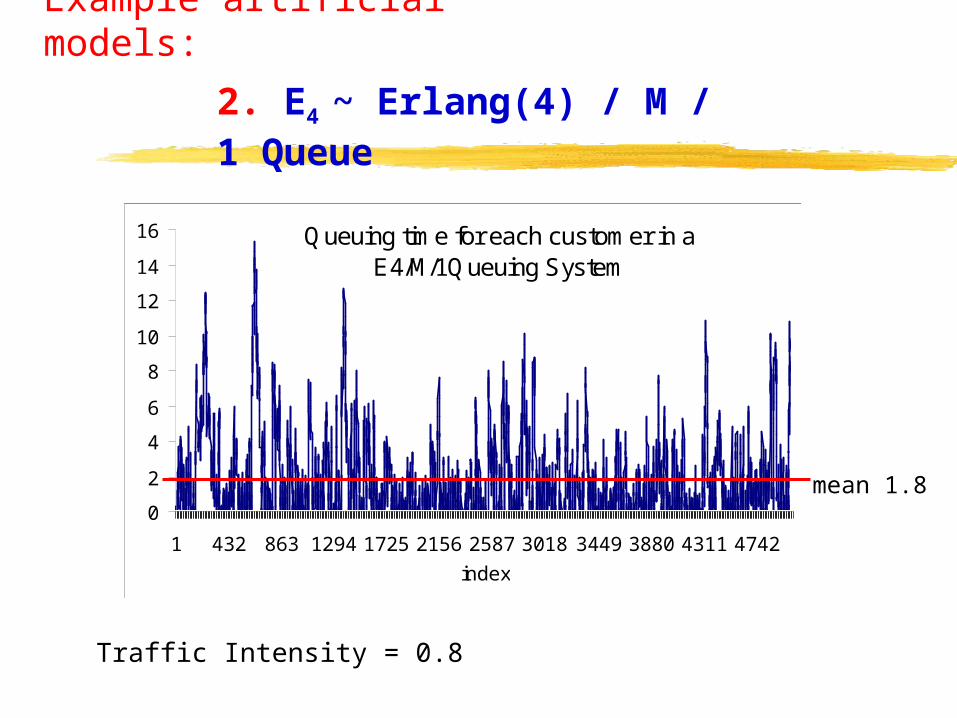
Example artificial models:

2. E4 ~ Erlang(4) / M / 1 Queue

Traffic Intensity = 0.8

Queuing time for each customer in a E4/M/1Queuing System

0

2

4

6

8

10

12

14

16

1 432 863 1294 1725 2156 2587 3018 3449 3880 4311 4742

index

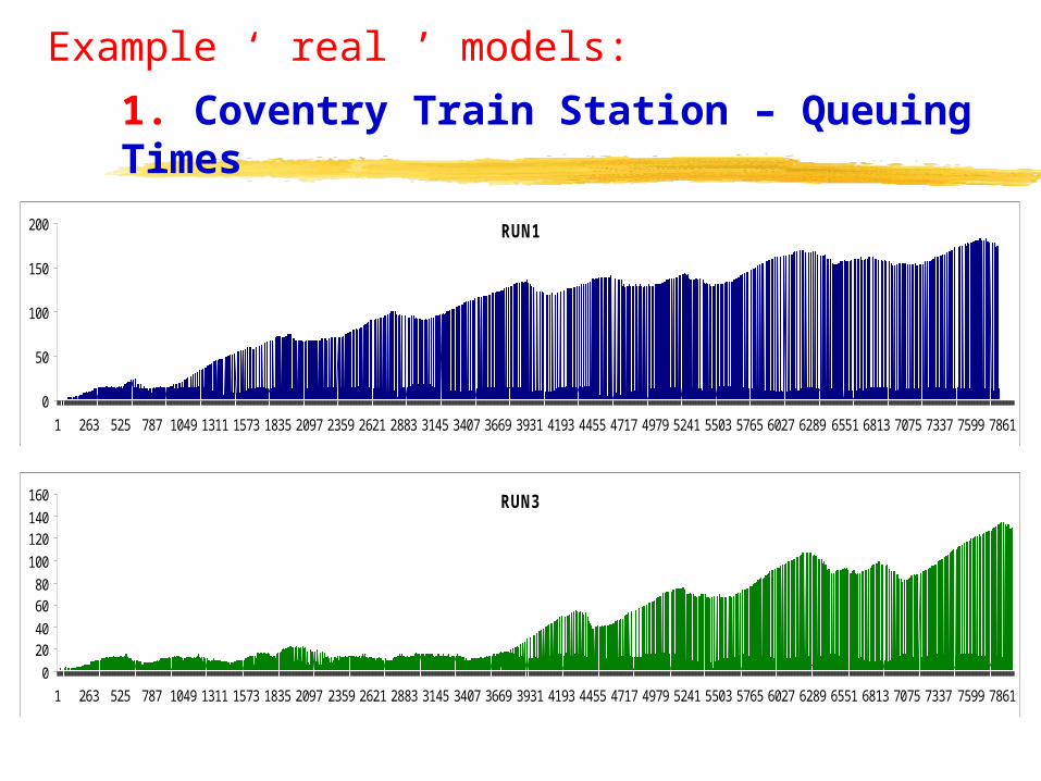
Example ‘ real ’ models:

1. Coventry Train Station – Queuing Times

RUN1

0

50

100

150

200

1 263 525 787 1049 1311 1573 1835 2097 2359 2621 2883 3145 3407 3669 3931 4193 4455 4717 4979 5241 5503 5765 6027 6289 6551 6813 7075 7337 7599 7861

RUN3

0

2040

6080

100

120140

160

1 263 525 787 1049 1311 1573 1835 2097 2359 2621 2883 3145 3407 3669 3931 4193 4455 4717 4979 5241 5503 5765 6027 6289 6551 6813 7075 7337 7599 7861

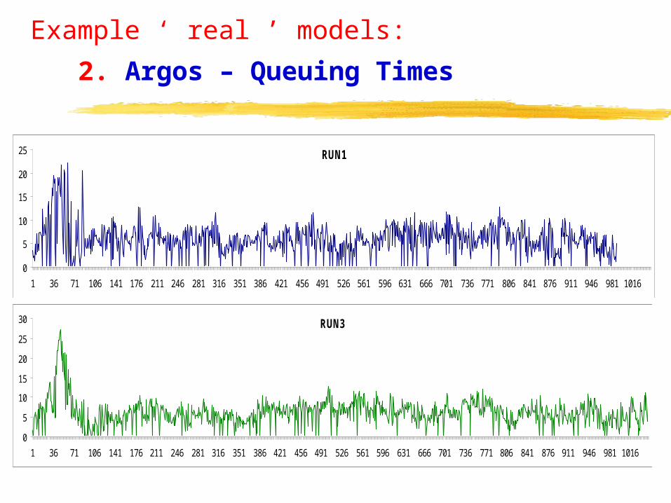
Example ‘ real ’ models:

2. Argos – Queuing Times

RUN1

0

5

10

15

20

25

1 36 71 106 141 176 211 246 281 316 351 386 421 456 491 526 561 596 631 666 701 736 771 806 841 876 911 946 981 1016

RUN3

0

5

10

15

20

25

30

1 36 71 106 141 176 211 246 281 316 351 386 421 456 491 526 561 596 631 666 701 736 771 806 841 876 911 946 981 1016

Example ‘ real ’ models:

3. Tesco petrol Station – Queuing Times

RUN1

0

5

10

15

20

1 186 371 556 741 926 1111 1296 1481 1666 1851 2036 2221 2406 2591 2776 2961 3146 3331 3516 3701 3886 4071 4256 4441 4626 4811 4996 5181 5366 5551

RUN3

0

5

10

15

20

1 185 369 553 737 921 1105 1289 1473 1657 1841 2025 2209 2393 2577 2761 2945 3129 3313 3497 3681 3865 4049 4233 4417 4601 4785 4969 5153 5337 5521

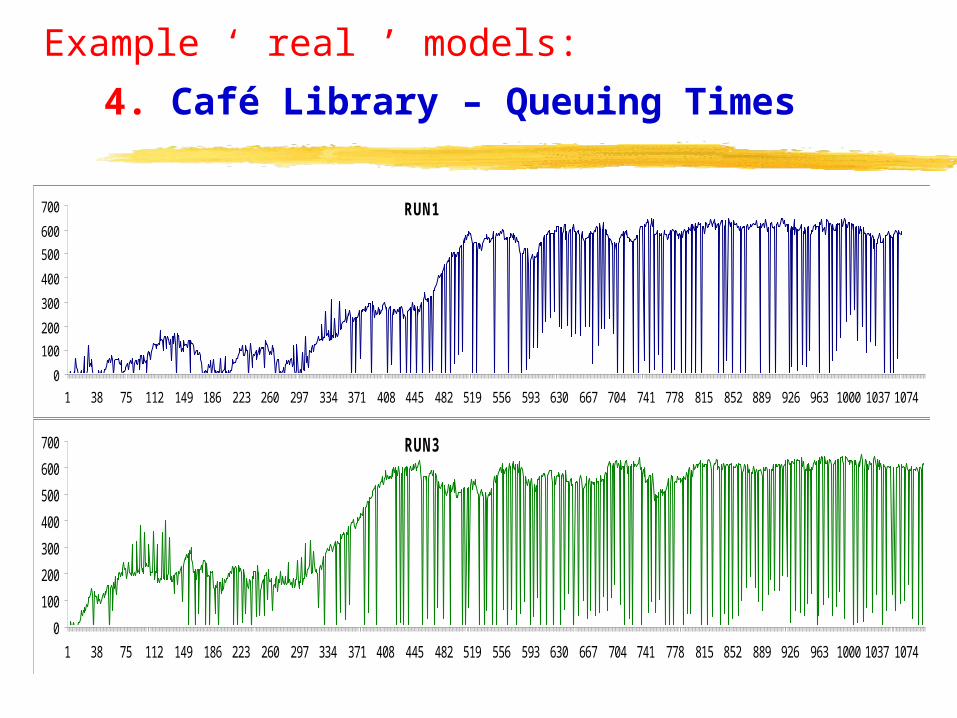
Example ‘ real ’ models:

4. Café Library – Queuing Times

RUN1

0

100

200

300

400

500

600

700

1 38 75 112 149 186 223 260 297 334 371 408 445 482 519 556 593 630 667 704 741 778 815 852 889 926 963 1000 1037 1074

RUN3

0

100

200

300

400

500

600

700

1 38 75 112 149 186 223 260 297 334 371 408 445 482 519 556 593 630 667 704 741 778 815 852 889 926 963 1000 1037 1074

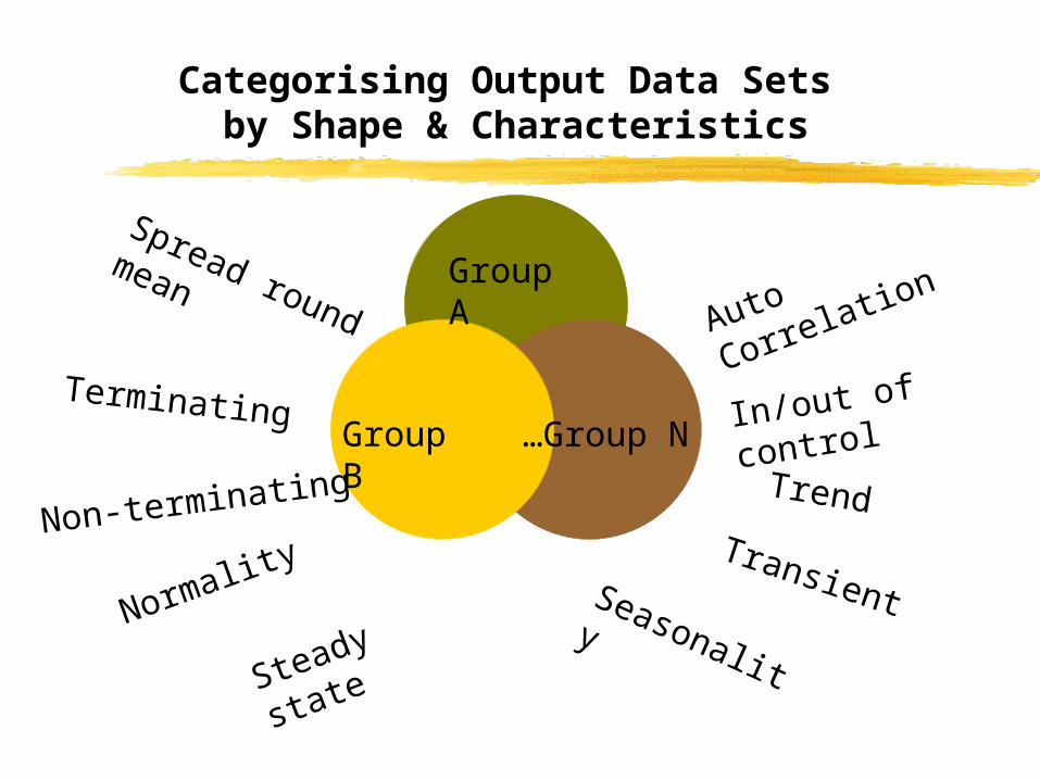
Categorising Output Data Sets by Shape & Characteristics

Group A

…Group NGroup B

Auto Correlation Spread round mean

Normality

Trend

Seasonality

Terminating

Non-terminating

Steady state

In/out of control

Transient