Embed Size (px)
Citation preview

Rochester Institute of Technology Rochester Institute of Technology
RIT Scholar Works RIT Scholar Works
Theses
4-28-2020
Automated brain segmentation methods for clinical quality MRI Automated brain segmentation methods for clinical quality MRI
and CT images and CT images
Viraj Reddy Adduru [email protected]
Follow this and additional works at: https://scholarworks.rit.edu/theses
Recommended Citation Recommended Citation Adduru, Viraj Reddy, "Automated brain segmentation methods for clinical quality MRI and CT images" (2020). Thesis. Rochester Institute of Technology. Accessed from
This Dissertation is brought to you for free and open access by RIT Scholar Works. It has been accepted for inclusion in Theses by an authorized administrator of RIT Scholar Works. For more information, please contact [email protected].

i
Automated brain segmentation methods for
clinical quality MRI and CT images
by
Viraj Reddy Adduru
B.Tech Jawaharlal Nehru Technological University, 2010
M.S. Rochester Institute of Technology, 2014
A dissertation submitted in partial fulfillment of the requirements for the
Degree of Doctor of Philosophy
in the Chester F. Carlson Center for Imaging Science
College of Science
Rochester Institute of technology
April 28th, 2020
Signature of the Author _______________________________________________
Accepted by ________________________________________________________
Coordinator, PhD. Degree Program Date

ii
CHESTER F. CARLSON CENTER FOR IMAGING SCIENCE
COLLEGE OF SCIENCE
ROCHESTER INSTITUTE OF TECHNOLOGY
ROCHESTER, NEW YORK
CERTIFICATE OF APPROVAL
Ph.D. DISSERTATION
The Ph.D. Degree Dissertation of Viraj Reddy Adduru
has been examined and approved by the
dissertation committee as satisfactory for the
dissertation requirement for the
Ph.D. degree in Imaging Science.
____________________________________
Dr. Andrew Michael, Dissertation Advisor
____________________________________
Dr. Stefi Baum, Dissertation Advisor
____________________________________
Dr. Maria Helguera, Academic Advisor
____________________________________
Dr. Linwei Wang, External Chair
____________________________________
Dr. Nathan Cahill, Committee Member
____________________________________
Date

iii
Automated brain segmentation methods for
clinical quality MRI and CT images
by
Viraj Reddy Adduru
Submitted to the
Chester F. Carlson Center for Imaging Science
in partial fulfillment of the requirements for the
Doctor of Philosophy Degree
at the Rochester Institute of Technology
Abstract
Alzheimer’s disease (AD) is a progressive neurodegenerative disorder associated with brain tissue
loss. Accurate estimation of this loss is critical for the diagnosis, prognosis, and tracking the
progression of AD. Structural magnetic resonance imaging (sMRI) and X-ray computed
tomography (CT) are widely used imaging modalities that help to in vivo map brain tissue
distributions. As manual image segmentations are tedious and time-consuming, automated
segmentation methods are increasingly applied to head MRI and head CT images to estimate brain
tissue volumes. However, existing automated methods can be applied only to images that have
high spatial resolution and their accuracy on heterogeneous low-quality clinical images has not
been tested. Further, automated brain tissue segmentation methods for CT are not available,
although CT is more widely acquired than MRI in the clinical setting. For these reasons, large
clinical imaging archives are unusable for research studies. In this work, we identify and develop
iv
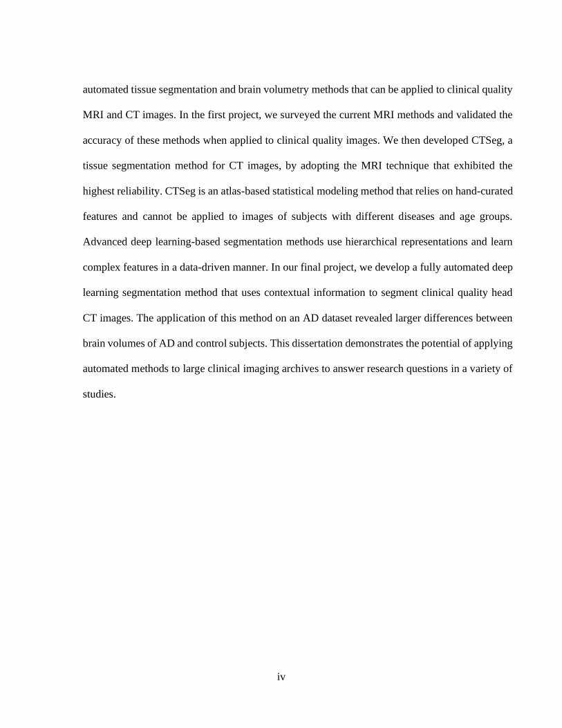
automated tissue segmentation and brain volumetry methods that can be applied to clinical quality
MRI and CT images. In the first project, we surveyed the current MRI methods and validated the
accuracy of these methods when applied to clinical quality images. We then developed CTSeg, a
tissue segmentation method for CT images, by adopting the MRI technique that exhibited the
highest reliability. CTSeg is an atlas-based statistical modeling method that relies on hand-curated
features and cannot be applied to images of subjects with different diseases and age groups.
Advanced deep learning-based segmentation methods use hierarchical representations and learn
complex features in a data-driven manner. In our final project, we develop a fully automated deep
learning segmentation method that uses contextual information to segment clinical quality head
CT images. The application of this method on an AD dataset revealed larger differences between
brain volumes of AD and control subjects. This dissertation demonstrates the potential of applying
automated methods to large clinical imaging archives to answer research questions in a variety of
studies.

v
Acknowledgments
As the last piece of writing that I have done for my PhD, a span of several years filled with a
variety of feelings and life lessons, I want to use this section to thank the wonderful people that I
met and had the pleasure to work with during these years.
First of all, I want to thank my advisor, Andrew M. Michael for his endless help and support,
without whom this work would be possible. I’m very fortunate to have known you Andrew and
have you as an advisor. You believed in me no matter what and gave me help in every possible
way to support me through this journey. You made sure that this work was always funded, which
played an enormous role by helping me focus on the important things. I can never forget the
patience and support you have demonstrated when there were delays in writing of the papers to
churn out all this research into words. It’s an honor to have worked under your guidance.
I thank my advisors Stefi Baum and Maria Helguera for their endless support and
encouragement they have given me, especially when I needed it the most. Their support and trust
in me kept my spirits high and kept me going. Critical research discussions with you all, especially
in the early stages of this work were the ones that shaped the trajectory of my research. I also want
to thank my committee members Nathan Cahill and Linwei Wang who were always kind, humble
and ready to give their time.
I’m very thankful to have had wonderful lab mates Gajendra, Chase and Chao during my days
in the beautiful town of Lewisburg. This journey would have been a tough one without them. All
the interesting conversations and fun we had will be among the memories I will cherish for the rest
of my life.

vi
My sincere gratitude goes to CIS and RIT for the academic and financial support throughout
my time as a student at RIT. I want to specially thank Elizabeth Lockwood, and Joyce French for
being on top of things and taking care of my academic requirements and made sure that I received
my stipend on time. My fellow PhD students: Shagan Sah, Bikash Basnet, Ritu Basnet, Chao
Zhang, Gajendra Katuwal with whom I had the immense pleasure and fun of learning together.
I want to thank Geisinger Health Systems for funding this research and letting us use its
valuable data that forms the foundation over which all my research work stands. I’m very thankful
for the time I did my PhD for all the wonderful resources, and communication tools I had at my
disposal as a student. The resources and experiences shared openly by the online research
community played a key role in my learning as a PhD student.
I thank Sadid Hassan under who’s guidance I had the pleasure of working during my internship
at Philips Research, Cambridge, Mass. Our discussions about ideas and possibilities of what we
could achieve inspired me and played a key role in shaping my career. I’m very grateful for the
opportunity to work with and know the best in the field.
Finally, I express my endless thanks to my parents, brother and wonderful friends who
supported me throughout this long and difficult journey. They gave me all the support and courage
to take the decisions that I have taken through this journey which ultimately shaped me into what
I am today. Importantly I want to thank Sowmya for being with me all these years and letting me
use the time that belonged to her, for my growth. Thank you for being with me during all the highs
and lows with your unconditional love.

vii
This thesis is dedicated to my teachers and my family

viii
Contents
1 Introduction ...............................................................................................................................1
2 Background ...............................................................................................................................6
2.1 Structural imaging of the human brain ........................................................................... 6
2.2 3D Brain Images ............................................................................................................. 7
2.3 Brain imaging applications in Alzheimer’s disease (AD) .............................................. 8
2.4 sMRI ............................................................................................................................. 10
2.5 CT Imaging ................................................................................................................... 14
2.6 Clinical imaging datasets .............................................................................................. 15
2.7 Brain Image Analysis .................................................................................................... 20
2.8 Segmentation using deep learning ................................................................................ 25
3 Reliability of automated brain segmentation methods on clinical quality MRI .....................31
3.1 Introduction ................................................................................................................... 31
3.2 Materials and Methods .................................................................................................. 32
3.3 Results ........................................................................................................................... 38
3.4 Discussion ..................................................................................................................... 46
4 CTSeg: A Probabilistic brain segmentation method for clinical quality head CT
images. ....................................................................................................................................49
4.1 Introduction ................................................................................................................... 49
4.2 Materials and Methods .................................................................................................. 51
4.3 Image Pre-processing .................................................................................................... 53
4.4 Results ........................................................................................................................... 60
4.5 Discussion ..................................................................................................................... 69
4.6 Conclusions ................................................................................................................... 73
5 Head CT segmentation using fully convolutional neural networks with spatial
context .....................................................................................................................................74
5.1 Introduction ................................................................................................................... 74
5.2 Materials ....................................................................................................................... 77

ix
5.3 Statistical Analysis ........................................................................................................ 82
5.4 Results ........................................................................................................................... 83
5.5 Discussion ..................................................................................................................... 93
5.6 Conclusion .................................................................................................................... 98
6 Conclusion ............................................................................................................................100
6.1 Contributions............................................................................................................... 100
6.2 Future work ................................................................................................................. 103
7 Bibliography .........................................................................................................................106

x
List of Figures
Figure 2.1 (A) Illustrates the three acquisition planes of the 3D structural brain image. (B) MRI
and (C) X-ray CT image of the human head in the three acquisition planes (Chudler,
2010). ............................................................................................................................................... 8
Figure 2.2 Illustration of the loss of brain volume at different stages of Alzheimer’s disease
(Frisoni et al. 2010). ......................................................................................................................... 9
Figure 2.3 (A) healthy and (B) AD patient brain MRI images showing global and hippocampal
atrophy (Smith et al., 2017)............................................................................................................ 10
Figure 2.4 Axial Slices (vertical) of a brain MRI image acquired using different scanner
parameters that highlight the contrast between different brain tissue types (Sweeney,
2016). ............................................................................................................................................. 13
Figure 2.5 (A) Illustration of CT image acquisition (Shivnauth et al., 2013). (B) Acquired CT
image in axial, sagittal and coronal planes..................................................................................... 14
Figure 2.6 (top row) Images containing different imaging artifacts. (Bottom row) Images
containing brains with abnormal pathology. .................................................................................. 18
Figure 2.7 Images assigned with different levels of grades for different levels of motion noise and
tissue contrast. ................................................................................................................................ 19
Figure 2.8 Brain tissues in a single section of a brain image. ..................................................................... 22
Figure 2.9 SPM brain segmentation pipeline illustrating probabilistic segmentation of GM, WM
and CSF and voxel based morphometry (Ashburner and Friston, 2012). ...................................... 24

xi
Figure 2.10 (left to right) The sigmoid, tanh and ReLU activation functions............................................. 28
Figure 2.11 Illustration of the max pooling operation. ............................................................................... 29
Figure 3.1 Flow chart of the inter-method brain volume comparison methodology between thick-
and thin-slice MR images. Green arrows represent the raw image input to three different
automated volume estimation methods: SPM, FreeSurfer, and FSL. Orange arrows
represent estimated brain volumes. The volume comparison box represents performing
statistical analyses to compare thick-slice and thin-slice image volumes. The inter-
method comparison box (gray box) represents the comparison of performance between
the three methods. .......................................................................................................................... 36
Figure 3.2 Scatter plots between thick-slice (y-axis) and thin-slice estimates (x-axis) of total brain
volume (TBV), gray matter volume (GMV), and white matter volume (WMV) as
estimated by three different automated methods: SPM, FreeSurfer and FSL. Blue lines
represent the trend lines fitted to the scatter points. Black lines represent the y=x reference
lines. ............................................................................................................................................... 41
Figure 3.3 Bland-Altman plots showing (thick – thin volume) difference (y-axis) plotted against
the respective mean value (x-axis) of thick and thin volumes for each subject for total
brain volume (TBV), gray matter volume (GMV) and white matter volume (WMV)
estimated by three automated volume estimation methods: SPM, FreeSurfer and FSL.
Solid blue line represents the trend lines. Numerical values of the mean difference (red
line) and ± 2 standard deviations (dashed blue line) are also presented. ....................................... 43
Figure 3.4 Effect of age on reliability. Intraclass correlation coefficient (ICC) (y-axis) between
thick- and thin-slice SPM estimates for total brain volume (TBV), gray matter volume

xii
(GMV) and white matter volume (WMV) as age (x-axis) of the oldest subject in the group
increases. The extreme left data points correspond to ICC for the ................................................ 44
Figure 3.5 Sagittal and axial views of intraclass correlation coefficient (ICC) between thick- and
thin-slice MR images in SPM voxel based morphometry for gray matter (in A) and white
matter (in B). All red regions represent fair to excellent agreement (ICC>0.37, P<0.01,
N=38) and all green regions represent insignificant ICC. The slice coordinates are in
Montreal Neurological Institute (MNI) space. ............................................................................... 46
Figure 4.1 CTSeg pipeline for intracranial space and brain parenchyma segmentation from head
CT images. Within parenthesis is the 3D coordinate space of the image. MNI: Montreal
Neurological Institute. .................................................................................................................... 55
Figure 4.2 Dice similarity index (DSI) computed for brain and intracranial binary masks of the
test subjects. ................................................................................................................................... 60
Figure 4.3 Axial views of head CT image slices for the three subjects that showed highest TBV
error. Top row of each subject is the original CT image viewed in brain intensity window
(40-80 Hounsfield Units) and second row is the binary brain mask of CTSeg overlaid on
top of manual segmentation mask and the original CT image slices. Brown represents
regions where CTSeg and the manual segmentations agree. Red regions represent false
positive labelling by CTSeg and green regions represent the false negatives. .............................. 62
Figure 4.4 Axial views of head CT images for the three subjects that showed the highest TIV
error. Top row of each subjects is the original CT image viewed in bone intensity window
(300-1500 Hounsfield Units) and second row is the binary intracranial mask from CTSeg
overlaid on top of manual segmentation mask and the original CT image. Brown regions
represent the voxels where the CTSeg and manual segmentations agree. Red regions

xiii
represent false positive labelling by CTSeg and green regions represent the false
negatives. ........................................................................................................................................ 63
Figure 4.5 (Top row) Scatter plots of automated vs manual volume estimates. Thin black line
represents the line of equality. Thick black lines represent the linear fit between
automated and manual volumes. (Bottom row) Bland-Altman plots presenting automated
minus manual volumes on y-axis and average of automated and manual volumes on x-
axis. Mean difference and ± 2 standard deviations (σ) are represented by dotted and
dashed horizontal lines respectively............................................................................................... 66
Figure 4.6 (left) Scatter plot of %TBV estimated using CTSeg maps vs age. (right) Scatter plot of
TBV vs TIV. Lines represent linear fits. ........................................................................................ 67

xiv
List of Tables
Table 3.1 Image and scanner parameters .................................................................................................... 34
Table 3.2 Summary of statistical analysis on thick and thin-slice volume estimations, for the three
automated methods: SPM (N = 38), FreeSurfer (N = 35) and FSL (N = 38). ............................... 39
Table 4.1 Image and Scanner parameters.................................................................................................... 53
Table 4.2 Comparison of automated TBV and TIV estimates with manual ground truth estimates.
........................................................................................................................................................ 65
Table 4.3 Results of linear regression analysis ........................................................................................... 68
Table 4.4 Segmentation failure rates of CTSeg pipeline for different scanners. ........................................ 69
Table 5.1 Segmentation performance of automated methods using validation data ................................... 84
Table 5.2 Comparison of volume estimations using automated methods from test set (N=8). .................. 89
Table 5.3 Comparison of %TBV estimates between Alzheimer’s(N=58) and control subjects
(N=58). ........................................................................................................................................... 93

1
Chapter 1
1 Introduction
STRUCTURAL BRAIN IMAGING
Structural brain imaging using magnetic resonance (MR) and computed tomography (CT)
modalities is capable of non-invasively mapping brain structure. In addition to visualizing brain
structure, these images are used to determine the volume of various anatomical regions inside the
brain. Quantifying the volumes of brain anatomical regions is referred to as brain volumetry
(Giorgio and De Stefano, 2013). Segmentation is the process of delineating the regions of interest
from the brain images and is an important tool for brain volumetry. Brain regions can be segmented
using manual or automated methods. Due to the time-consuming and tedious nature of the manual
methods, automated methods are increasingly used for brain volumetry.
BRAIN VOLUMETRY IN ALZHEIMER’S DISEASE
AD is an irreversible, progressive neurodegenerative disorder resulting in loss of brain tissue
volume. It is the most common form of dementia. As of 2017, one person develops dementia every

2
66 seconds in the USA (Yolanda Smith, 2017). This rate is expected to double by 2050.
Neuroimaging studies report that regional brain volume loss starts as early as five years before
symptoms are evident (Johnson et al., 2012). Accurate early identification of brain tissue loss
(atrophy) using automated brain volumetry allows for early clinical intervention and aids in
slowing down disease progression. Recent advances in brain image processing and volumetry
methods not only detect atrophy at an early stage, called mild cognitive impairment (MCI), but
also predict the patients that are likely to advance to AD (Jack et al., 2010; McEvoy et al., 2011).
Therefore, the disease can be controlled, if not prevented, if the disease is detected in the early
stages. Brain volumetry using automated methods is an important tool for diagnosis, prognosis,
and tracking the progression of Alzheimer’s disease (AD) (Johnson et al., 2012) and other
neurodegenerative diseases. Automated methods that are capable of tracking atrophy using
clinically acquired brain images collected at different timepoints of the same patient are desirable
for early detection of AD.
RELIABILITY OF AUTOMATED METHODS
The accuracy of the methods that use brain volumetry depends on the accuracy of the automated
segmentation methods being used. This raises important questions about the reproducibility of
research studies that rely on the segmentation methods (Maclaren et al., 2014). Current widely
used brain segmentation methods are developed and validated using high-quality images acquired
for research purposes. Their reproducibility has not been validated on clinical quality images that
are heterogeneous in image quality, scanner model, brain abnormalities, medical conditions,
motion and other factors.

3
RESEARCH VS CLINICAL QUALITY IMAGING
Unlike research-quality images which are homogenous, as they are collected using advanced
image acquisition protocols and by following strict quality-control, clinical-quality images are
heterogenous. Research hospitals maintain large archives of (tens of thousands) images obtained
for diagnostic purposes using standard-of-care acquisition protocols. These images are consented
for research studies after deidentification by removing patient-specific information. These datasets
are a great resource to obtain a deeper understanding of various medical conditions. However,
clinical images are highly heterogenous and exhibit a wide range of image quality, medical
conditions, and patient demographics. The clinical-quality images are typically acquired at lower
resolutions (thick slices) to aid in better tissue contrast, faster acquisition times, and lower costs.
Other additional issues with clinical images are low contrast-to-noise ratio, resolution, the presence
of artifacts and the presence of brain abnormalities.
Conventional machine learning based segmentation methods require careful engineering and
domain expertise to select imaging features to detect or segment a region of interest (LeCun et al.,
2015). Due to the heterogenous nature of the clinical-quality imaging data it is extremely difficult
to engineer these features. Therefore, automating the feature engineering process is highly
desirable for developing robust segmentation methods.
DEEP LEARNING
Recent advancements in deep learning methods like convolutional neural networks (CNNs) are
data-driven i.e. they automatically learn complex features required for segmentation directly from
the data (LeCun et al., 2015). However, these methods require large datasets with ground truth
labels, computationally intensive, and difficult to train. Recent advances in computer technologies
4
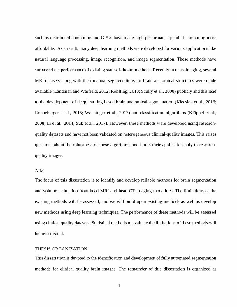
such as distributed computing and GPUs have made high-performance parallel computing more
affordable. As a result, many deep learning methods were developed for various applications like
natural language processing, image recognition, and image segmentation. These methods have
surpassed the performance of existing state-of-the-art methods. Recently in neuroimaging, several
MRI datasets along with their manual segmentations for brain anatomical structures were made
available (Landman and Warfield, 2012; Rohlfing, 2010; Scully et al., 2008) publicly and this lead
to the development of deep learning based brain anatomical segmentation (Kleesiek et al., 2016;
Ronneberger et al., 2015; Wachinger et al., 2017) and classification algorithms (Klöppel et al.,
2008; Li et al., 2014; Suk et al., 2017). However, these methods were developed using research-
quality datasets and have not been validated on heterogeneous clinical-quality images. This raises
questions about the robustness of these algorithms and limits their application only to research-
quality images.
AIM
The focus of this dissertation is to identify and develop reliable methods for brain segmentation
and volume estimation from head MRI and head CT imaging modalities. The limitations of the
existing methods will be assessed, and we will build upon existing methods as well as develop
new methods using deep learning techniques. The performance of these methods will be assessed
using clinical quality datasets. Statistical methods to evaluate the limitations of these methods will
be investigated.
THESIS ORGANIZATION
This dissertation is devoted to the identification and development of fully automated segmentation
methods for clinical quality brain images. The remainder of this dissertation is organized as

5
follows. Chapter 2 contains basic concepts and introduce the current state-of-the-art followed by
advanced methods that will be frequently used in this thesis. Chapter 3 analyses the reliability of
existing fully automated brain segmentation methods on clinical quality brain MRIs. The
performance of three widely used MRI segmentation methods are compared between clinical- and
research-quality images of the same subjects. Chapter 4 presents a novel CT segmentation pipeline
developed by adapting an existing widely used atlas-based MRI segmentation method and
demonstrates its application in the detection of atrophy in Alzheimer’s disease patients. Chapter 5
presents a novel deep learning architecture using CNN that is designed to overcome the
shortcomings of the atlas-based CT segmentation method. In chapter 6 we conclude by presenting
key contributions of this work and discuss potential future work.

6
Chapter 2
2 Background
This chapter provides an understanding of the structural brain imaging of the human brain using
sMRI and CT imaging modalities. Later, we discuss the process of cleaning the clinical imaging
data and preparing them for research purposes. Clinical images are highly heterogenous and should
be subjected to strict quality control at various stages. The quality control strategies that were
employed in this work will be discussed here. Then we introduce several existing widely used
image preprocessing and analysis methods for segmentation and volume estimation of brain
regions from 3D brain images. Challenges related to application of these methods on clinical
quality images will be discussed. New segmentation methods using advanced artificial neural
networks will be discussed. Finally, we will present the application of brain segmentation methods
for Alzheimer’s Disease applications.
2.1 Structural imaging of the human brain
Structural imaging of the brain involves in vivo imaging of the structure of the human nervous
system. There are several technologies available to create brain images: MRI, CT, positron
emission tomography (PET), electroencephalography (EEG), Magnetoencephalography (MEG)
and near infrared spectroscopy (NIRS) (Michael Demitri, 2018). Of these technologies, structural
MRI (sMRI) and CT are the widely used modalities for imaging the human brain for both research
and clinical purposes. 3D and 2D images can be acquired using sMRI and CT imaging modalities.

7
Structural brain imaging is increasingly used to study the brain structure in research and
clinical applications for disease diagnosis, prognosis and to monitor treatment effects (Giorgio and
De Stefano, 2013). There are numerous other applications of structural brain imaging, one of them,
which is the major focus of this work, is brain volumetry. Brain volumetry involves quantifying
various anatomical regions of the brain like gray matter (GM), white matter (WM), cerebrospinal
fluid (CSF), intracranial space and subcortical structures like amygdala, hippocampus etc.
2.2 3D Brain Images
Every 3D sMRI or CT image consists of a 3D array of elements called voxels. A voxel is a cuboidal
volume encompassing a 3D volume in space. The voxel size is determined by the length, width
and height of the cuboid. Each voxel is assigned a value that represents the intensity of the
encompassed 3D space. The dimensions of these voxels (length, width and height) in the sMRI or
CT imaging methods, are determined by the acquisition parameters set during scanning and the
intensity value at each voxel represents the average signal intensity received from the physical
volume imaged inside the voxel.
In practice, sMRI and CT images are acquired in planar sections: coronal, axial, and sagittal,
on which the voxels are arranged in a 2D grid (Figure 2.1 A) along the x and y axes, just like pixels
in an image. Figure 2.1 B and C illustrate MRI and CT sections, respectively, acquired in different
acquisition planes. These 2D sections of voxels are arranged along an orthogonal grid along the z
axis (orthogonal to x and y axes) making the image a 3D image.

8
Figure 2.1 (A) Illustrates the three acquisition planes of the 3D structural brain image. (B) MRI
and (C) X-ray CT image of the human head in the three acquisition planes.
2.3 Brain imaging applications in Alzheimer’s disease (AD)
Diagnosis of AD is typically made by neuropsychological and neuroimaging assessment.
Neuroimaging is routinely used for assessment of brain atrophy in AD patients to track disease
progression. Neuroimaging studies in AD have shown that the brain exhibits atrophy in various
regions up to 5 years before the diagnosis (Chan et al., 2003). Figure 2.2 illustrates the loss of
volume in various brain regions as the disease progresses through the three stages: asymptomatic,
MCI and dementia. Hippocampal and entorhinal volumes show a loss of 15-25% of overall volume
at the time of diagnosis (Chan et al., 2001). The volume and the rate of brain volume loss in these
regions can be quantified using brain images acquired at different timepoints from the same
patient. Hence imaging has prognostic capabilities which can lead to early diagnosis of AD.

9
Figure 2.2 Illustration of the loss of brain volume at different stages of Alzheimer’s disease
(Frisoni et al., 2010).
MRI is the preferred neuroimaging modality for AD because of its ability to distinguish various
anatomical regions inside the brain like Hippocampus. Though not as fast as a CT, a high-
resolution volumetric scan can be acquired in 5-10 mins using MRI. MRI is safe and doesn’t
involve exposure to harmful radiation and therefore individuals can be imaged for routine checks
without any concerns about the harmful side effects.
In a typical imaging protocol for AD diagnosis, patients are imaged with CT and then followed-
up by MRI to rule out other causes of dementia (Johnson et al., 2012). Although CT may not be

10
used for primary diagnosis of the disease, cerebral atrophy (loss of whole brain volume) which is
typical of advanced AD can be detected using CT. Figure 2.3 compares the MRI image of an AD
patient with a healthy subject illustrating cerebral atrophy in addition to loss of volume in
hippocampus and both the left and right lobes.. Hence CT is sometimes recommended for the
routine evaluation of AD. CT is preferred over MR when MR is contraindicated, not readily
available or not affordable (Petrella, 2003).
Figure 2.3 (A) healthy and (B) AD patient brain MRI images showing global and hippocampal
atrophy (Duara et al., 2008).
2.4 sMRI
sMRI is a widely used medical imaging modality for both research and clinical applications. About
20,000 research articles are published on MRI every year (Vlaardingerbroek and Boer, 2013).
Applications of sMRI covers every part of the human body from head to toe and it is used in a
wide variety of diseases such as stroke, cancer, and AD. One main advantage of MR is that there

11
are no reported side effects on the human body. Since its introduction in the 1980s MR imaging
has improved in image quality and resolution enabling it to create detailed representations of the
tissues inside the human body.
Figure 2.4 (a) Illustration of the MRI image acquisition system. (b) Illustration of the gradient coils
in all three dimensions. Transceiver consists of a transmitter, coil and receiver (Coyne, 2012).
MRI machine (Figure 2.4a) consists of a large magnet that maintains a constant magnetization all
through its core and small gradient coils that create a gradient magnetic field along each of the
three axes. The strong magnetization aligns the spins of the protons present in the body that we are
interested in imaging, perpendicular to the direction of the magnetization. The gradient magnetic
coils (Figure 2.4b) are used for spatial encoding of the MRI signal by making the protons precess
at slightly different rates. Phase and frequency encoding is achieved using the gradient magnetic
fields which encode the RF signals coming from different regions of the 3D space thereby
providing the RF receiver with a spatial information to reconstruct the 3D image.
A 3D sMRI is created by stacking a number of 2D sections or slices each containing a matrix
of voxels. The intensity values of the voxels in the sMRI images are unitless. sMRI is acquired
using a combination of settings, called pulse sequences. Every sequence is designed to achieve the
12
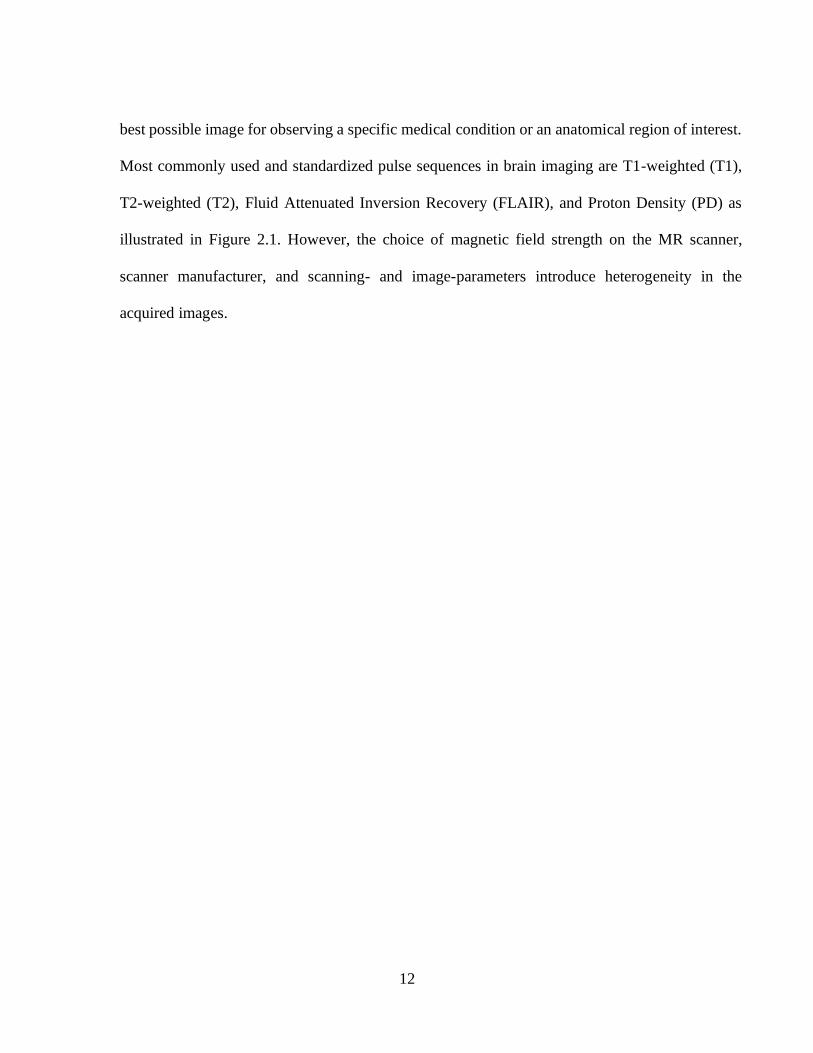
best possible image for observing a specific medical condition or an anatomical region of interest.
Most commonly used and standardized pulse sequences in brain imaging are T1-weighted (T1),
T2-weighted (T2), Fluid Attenuated Inversion Recovery (FLAIR), and Proton Density (PD) as
illustrated in Figure 2.1. However, the choice of magnetic field strength on the MR scanner,
scanner manufacturer, and scanning- and image-parameters introduce heterogeneity in the
acquired images.

13
Figure 2.5 Axial slices (vertical) of a brain MRI image acquired using different scanner parameters
that highlight the contrast between different brain tissue types (Sweeney, 2016).
In spite of MRI being a great imaging tool with no reported side effects, in a clinical setting it
is not as widely used as CT due to several reasons; MRI is very expensive to acquire and takes
longer scanning time which leads to high operating costs. Due to the large magnetization, people
who have metal implants or shrapnel cannot have an MRI.

14
2.5 CT Imaging
X-ray Computed Tomography (CT) is the most widely used modality for imaging in the clinical
setting. Compared to MRI, CT has lower cost, faster acquisition, and fewer contraindications, as
well as reasonable image quality making CT applicable for a plethora of medical conditions and
situations. Therefore, CT is the imaging modality of choice in case of emergencies. However, CT
exposes the patient to a dose of ionizing radiation which is associated with side effects and
complications. This makes it difficult to justify its use in a research setting especially for obtaining
brain images from healthy volunteers. Hence, CT is used mostly only in a clinical setting when the
procedure is essential for diagnostic purposes.
Figure 2.6 (A) Illustration of CT image acquisition (Shivnauth et al., 2013). (B) Acquired CT
image viewed in the tissue intensity window (0-100Hu) in axial, sagittal and coronal planes.
Although CT brain image also consists of an array of 3D voxels just like MRI, the method of
acquisition is quite different. CT takes advantage of the X-ray attenuation property of the tissues.
The intensity of each voxel is the measure of X-ray attenuation in Hounsfield units (HU) of the
15
physical medium enclosed by the voxel. Therefore, the voxel intensity is consistent irrespective of
the scanner and scanner brand. In contrast to MR, CT exhibits a low contrast-to-noise ratio between
soft tissues like GM and WM regions of the brain. For dense tissues like bone, the attenuation is
very high therefore the intensity of such structures in a CT image is very high compared to the soft
tissues. Therefore, it is very hard to distinguish soft tissues like GM, WM and other subcortical
structures in a CT brain image. Unlike MRI the freedom of selecting the axis of imaging in CT
images is limited. The axis is determined by the angle of the CT imager gantry. The gantry is
usually perpendicular to the axial axis of the head when acquiring axial slices of the head.
However, sometimes gantry is tilted to avoid the artifacts due to bone in CT images resulting in
the slices that are tilted at an angle but still acquired along the axial direction. The range of the tilt
angle is very limited due to the physical constraints.
The scope of the research in this work is limited to the 3D structural imaging of the brain.
Henceforth for the rest of the dissertation MRI refers to the 3D sMRI and CT refers to 3D X-ray
CT. All the MRI images used in this work are T1-weighted MRI images. Both MRI and CT
datasets used in this work consist of images acquired from patients of a large hospital system
acquired for diagnostic purposes using standard-of-care imaging practices.
2.6 Clinical imaging datasets
Clinical datasets are a collection of images that are obtained from the imaging archives of a hospital
that are primarily acquired for diagnostic purposes. These images are acquired using standard-of-
care procedures. Clinical images are originally ordered by a physician for diagnosing a condition
and the image parameters for the acquisition are chosen by the operator to best capture the region
of interest.

16
Clinical quality image datasets in this work were created from images available in Geisinger
Health System’s clinical picture archiving and communication system (PACS). MRI and CT
images obtained from the archives were de-identified (i.e. removal of all protected health
information (PHI) to comply with HIPAA regulations). The data access for the research studies in
this work was approved by Geisinger’s institutional Review Board. Preparation of datasets using
these images and handling of the image files is described below.
2.6.1 Preparing Clinical Quality Brain Images
Clinical-quality images are highly heterogeneous with respect to image parameters, subject age,
diagnosis, etc. Due to this heterogeneity, the datasets prepared by collecting these images should
be subjected to strict quality checks at different stages. The process we used for obtaining the
imaging dataset, preparation of the clinical datasets, and post processing quality assessment is
outlined in this section.
The images obtained from PACS come in the Digital Imaging and Communications in
Medicine (DICOM) format containing one DICOM file per image slice. DICOM files contain
image intensity data along with a large amount of metadata which includes information about
image acquisition, type of scan, scanning equipment information, patient and image parameters
etc. This overhead of metadata makes the DICOM images less portable for research. Further, for
research questions we require only a small number of those variables, mainly the intensity matrix
and imaging parameters. Therefore, in research, the practice is to convert the images from the
DICOM format to the Neuroimaging Informatics Technology Initiative (NIfTI) format (Cox et al.,
2004). This format is lighter and simpler to use and includes sufficient information to process the
images.

17
Creating Clinical datasets starts with selecting DICOM images of patients that satisfy
specific criteria that we are interested in for a study (for example: patients from age 60 to 80 years
diagnosed with AD). This is followed by a two-step quality check in which images with
undesirable structural abnormalities and artifacts are removed.
2.6.2 Pre-processing quality check
Clinical images may contain abnormalities that are visibly present like motion artifacts,
implants, noise, cancerous growth, hemorrhage, abnormal brain conditions etc. Some of the
common image artifacts and brain abnormalities are presented in Figure 2.7. These abnormalities,
if they are not part of the study, create undesirable noise and biases during analysis. Therefore, it
is very important that a rigorous quality check is done to remove such images and grade the
remaining images for quality before any analysis methods are applied. This grading helps us
understand the performance of analysis methods when applied on images with different quality
grades. This quality check is a two-step process as outlined below.
Step1. In this step the images undergo a careful visual inspection to exclude the images that
contain abnormalities that do not concern the research question. This visual inspection should be
performed under the supervision of an experienced neuro-radiologist. This step reduces the
undesirable heterogeneity in the image dataset.

18
Figure 2.7 (top row) Images containing different imaging artifacts. (Bottom row) Images
containing brains with abnormal pathology.
Step 2. After the removal of images with artifacts and brain abnormalities, the images undergo
a second visual inspection to grade them according to the quality of the tissue reconstruction. In
this step the images are visually examined for signal to noise ratio, tissue contrast to noise and
graded into three categories: grade 0 or ‘low’ quality, grade 1 for ‘good’ quality and grade 2 for
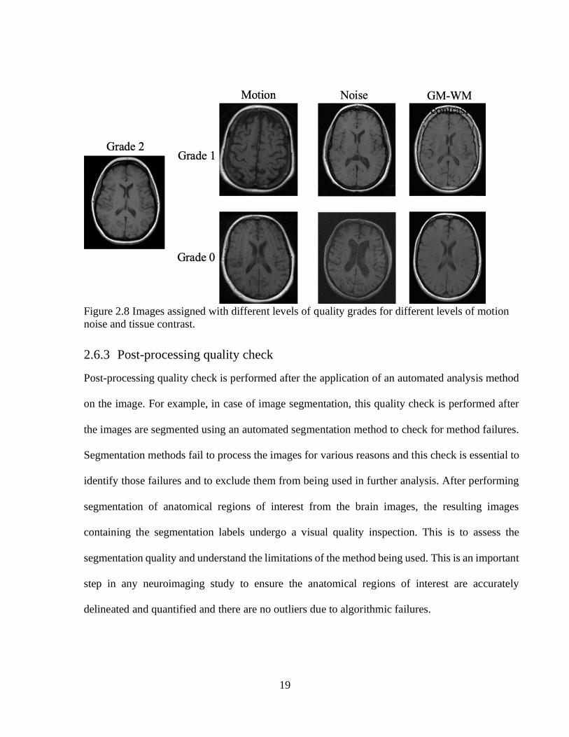
‘high’ quality. Figure 2.8 illustrates brain images with different levels of motion, noise and tissue
contrast and the grades assigned to them. This quality rating helps us to understand the influence
of image quality on study results. This method of grading is qualitative, and subjective and should
be performed only by a trained operator. Although some image quality metrics like signal-to-noise
ratio can be measured, there is no standard criteria to grade these images.
19
Figure 2.8 Images assigned with different levels of quality grades for different levels of motion
noise and tissue contrast.
2.6.3 Post-processing quality check
Post-processing quality check is performed after the application of an automated analysis method
on the image. For example, in case of image segmentation, this quality check is performed after
the images are segmented using an automated segmentation method to check for method failures.
Segmentation methods fail to process the images for various reasons and this check is essential to
identify those failures and to exclude them from being used in further analysis. After performing
segmentation of anatomical regions of interest from the brain images, the resulting images
containing the segmentation labels undergo a visual quality inspection. This is to assess the
segmentation quality and understand the limitations of the method being used. This is an important
step in any neuroimaging study to ensure the anatomical regions of interest are accurately
delineated and quantified and there are no outliers due to algorithmic failures.

20
2.7 Brain Image Analysis
2.7.1 Brain volumetry
Brain volumetry typically involves segmentation and quantification of various tissue types of the
brain such as GM, WM and CSF. Other Global metrics include total intracranial volume (TIV)
and total brain volume (TBV) which are volume estimates of the intracranial space and the brain
parenchyma respectively. These metrics are called global metrics as they are computed for the
brain as a whole which includes the brain cortex, subcortical regions, cerebellum, brainstem and
for TIV the fluid surrounding these structures. Regional brain volume metrics comprise of volumes
of anatomical brain structures like hippocampus, amygdala, thalamus, nucleus accumbens, etc
which constitute the subcortical structures. Other types of regional brain volumes measures include
lobes and regions that represent various functions like speech, vision, memory etc.
The volume of a brain tissue is measured by integrating the volumes of the voxels belonging
to the region of interest in a structural image. These regions of interest are segmented using manual
or automated methods. Manual brain segmentation is performed by individuals with training in
brain anatomy with the aid of MRI visualization software tools. This is a laborious procedure
which results in inter and intra-operator variability of the estimated volume. Nordenskjöld et al.,
(2013) reported that manual segmentation of TIV of a brain image with 50 image slices can take
up to 25 minutes for an experienced operator. Therefore, automated tools are increasingly used for
brain volumetry. A wide variety of automated methods are available for the segmentation of brain
images. A study by Helms, (2016) provides an extensive review of the available state-of-the-art
brain segmentation methods.

21
The whole brain volume metrics are directly computed from the brain images by identifying
the voxels within the intensity range of the tissues. Whereas the regional brain volumes are
computed from the voxels delineated by identifying complex region boundaries that make these
regional structures. In practice, the voxels belonging to these complex brain structures are
identified by carefully registering standard brain atlases onto the brain image. Most of the work in
this thesis is focused on accurately estimating global brain volumes.
2.7.2 Automated Brain Image Segmentation
Brain segmentation involves accurately delineating the brain images into different tissues: GM,
WM, and CSF (Figure 2.9). A variety of automated segmentation methods currently exist of which
Statistical Parametric Mapping (SPM) (Ashburner and Friston, 2005), FreeSurfer
(surfer.nmr.mgh.harvard.edu/) (Dale et al., 1999; Fischl et al., 2002a), and FMRIB Software
Library (FSL) (https://fsl.fmrib.ox.ac.uk/fsl) (Smith et al., 2004) are the most widely used. This
section outlines the brain segmentation methodology used by each of these automated methods.

22
Figure 2.9 Brain tissues in a single section of a brain image from (A.) an MRI image, (B.)an
average MRI brain tissue probabilistic map.
STATISTICAL PARAMETRIC MAPPING (SPM)
SPM uses an atlas-based Bayesian method to perform brain segmentation. SPM starts by
registering the subject’s brain image onto a tissue probability map (TPM). TPM contains prior
probability maps of different tissue classes of the voxels in the standard space template. For linear
and non-linear registration SPM uses a default International Consortium for Brain Mapping space
template (ICBM; Rex et al., 2003) whose coordinates are defined in the Montreal Neurological
Institute (MNI) space. The unified segmentation algorithm also accounts for any biases present in
the image intensity. The segmentation algorithm performs tissue classification, bias correction and
registration steps iteratively to optimize the parameters for maximum a posteriori solution.

23
The above segmentation yields three types of images: (1) probabilistic tissue maps in the native
space of the subject, (2) probabilistic tissue intensity maps in the template space and (3) modulated
tissue intensity maps in the template space (Figure 2.10). The modulated images preserve the local
volumetric changes in grey and white matter intensity on a voxel-by-voxel basis while spatially
normalizing to the template. The modulated images are used for voxel-based morphometry (VBM)
(Ashburner and Friston, 2000) as they measure subtle changes in the anatomical brain structures
by removing the global affine effects (like scaling, rotation and translation). GM volume (GMV)
and WM volume (WMV) are obtained by integrating the product of the corresponding tissue
probabilities and the voxel volume in the native space of the subject. We will be using VBM to
estimate the volumes of subcortical structures of the brain in chapter 3.

24
Figure 2.10 SPM brain segmentation pipeline illustrating probabilistic segmentation of GM, WM
and CSF and voxel based morphometry (Ashburner and Friston, 2012).
FREESURFER
FreeSurfer utilizes a complex fully automated segmentation method for segmenting the brain into
various cortical and subcortical regions (Fischl et al., 2002a). Segmentation is done by modeling
a segment as an anisotropic Markov random field by using the priors for anatomical regions which
are obtained after registering the image onto a template. FreeSurfer uses recon-all pipeline for
segmentation, which also includes several preprocessing stages such as motion correction, non-
uniform intensity normalization, Talairach transform computation, intensity normalization, skull
stripping, and cortical parcellation. In addition to volumetric analysis FreeSurfer also provides

25
surface-based analysis of the brain. It creates a vertex map for surfaces which forms the interfaces
(e.g., WM-GM, GM-CSF) between different soft tissues.
FMRIB SOFTWARE LIBRARY (FSL)
FSL uses the SIENAX algorithm to perform brain extraction and tissue segmentation. SIENAX
first creates a brain mask for the T1 image using FSL’s brain extraction tool (BET) (Jenkinson et
al., 2002b). BET performs brain segmentation by growing a tessellated mesh inside the cranium
until the boundary between brain and CSF is reached. After brain extraction, brain tissues are
segmented using FSL’s Automated Segmentation Tool (FAST) (Zhang et al., 2001). FAST uses
hidden Markov random field segmentation with expectation maximization algorithm and segments
the brain into GM and WM segmentations.
2.8 Segmentation using deep learning
One of the important steps in brain segmentation is the feature learning. These features represent
the patterns for identifying region boundaries for detecting various structures like GM, WM and
CSF. In atlas-based methods as discussed above the probabilistic tissue maps are the examples of
these features which determine the soft tissues in the brain. These probabilistic tissue maps created
using manually segmented tissue maps which require careful delineation of the tissues from good
quality healthy brain images or using statistical methods that rely on manually selected features.
These features are highly task dependent and different task requires deriving a set of new features.
For example, the probabilistic tissue maps that are used for segmenting healthy brains of a certain
age cannot be used for segmenting images that have artifacts, certain brain conditions or from a
different age group. Furthermore, curating these features requires a lot of domain knowledge that

26
is very difficult to obtain in many cases. Therefore, data-driven methods that can automatically
learn these features from the ground truth data are highly desirable for developing robust
segmentation methods. As segmenting brain structures involves identification of complex features
that can be derived from a combination of simpler features, having a hierarchical feature learning
setup is much more efficient.
Although deep learning dates back to 1980’s, only in the recent years has gained popularity
due to the advances in neural networks and availability of large computing power. Deep learning
neural network architecture consists of layers of neural networks that are stacked to form a larger
neural network. With more layers the network can learn more complex representations.
2.8.1 Convolution neural networks
CONVOLUTION
Convolution neural network (CNNs) (Krizhevsky et al., 2012; LeCun et al., 1998) is a special kind
of neural network in which each layer consists of filters, also called kernels, that convolve with
the input data and computes features or representations. These features are fed to the consecutive
layers which have another set of filters to learn hierarchical representations and so forth. Kernels
may be of 2D for 2D images or 3D for 3D images and consist of weights. Weights are
automatically learned by training the model using the ground truth data. Convolution neural
networks are suitable for data that are arranged in grid-like fashion and contain sparse but repeated
features e.g. images.
Discrete convolution is defined as follows:
𝑆(𝑖, 𝑗) = (𝐼 ∗ 𝐾)(𝑖, 𝑗) = ∑ ∑ 𝐼(𝑚, 𝑛) × 𝐾(𝑖 − 𝑚, 𝑗 − 𝑛)
𝑛𝑚

27
Where I is the input signal/image, K is the convolutional kernel and the output S is called the
feature map. The three important properties that help CNNs to perform well over conventional
neural networks are sparsity, parameter sharing and shift invariance (Goodfellow et al., 2016).
These properties are elaborated below briefly to support the usage of CNNs for segmentation.
SPARSITY:
The values of the features in CNNs are computed over the entire input image by advancing the
kernel from start to end along all the dimensions. Each value in the feature map is obtained by the
neighborhood around it and it’s the same as the size of the kernel being used. The kernel size is
usually selected much smaller than the input size resulting in a finite number of advances along
each dimension resulting in a feature size with same number of dimensions as the input although
the size is different. Smaller size of the kernel provides a number of advantages: reduced memory
requirement, decreased computational costs and statistical efficiency.
PARAMETER SHARING:
As convolution operation is performed by advancing the kernel over the input, the weights in the
kernel are used multiple times resulting in weight sharing. Contrastingly in conventional neural
networks each weight is only used once to compute the feature values. This results in substantial
reduction in number of parameters in the neural network there by reducing its memory footprint.
SHIFT INVARIANCE:
CNNs are shift (also called translation) invariant which means that when the image is shifted,
convolving that input with the kernel produces a shifted feature output. Therefore, the same kernel
is capable of detecting the same features wherever it is present in the image. However,

28
convolutions are sensitive to other image operations like rotation, scaling and shearing (Figure
2.11).
Figure 2.11 Illustration of different operations performed on images.
ACTIVATION FUNCTIONS
At the end of each layer in a CNN non-linearities are introduced in the output feature maps using
the activation functions. Without non-linearity any number of neural networks connected one after
the other can be solved using a single shallow neural network. The main advantage of deep neural
networks is creating hierarchical features which can only be accomplished by introducing a
nonlinearity after every layer. Most common activation functions used in CNNs are sigmoid, tanh,
and rectified linear unit (ReLU). Sigmoid and tanh activation functions have a disadvantage of
diminishing the gradients in the shallower layers during the back-propagation which slows down
the learning. Therefore, ReLU is the recommended nonlinear activation function in neural
networks containing multiple layers. In addition to avoiding the vanishing gradient problem, ReLU
also contributes to the computational efficiency.
Figure 2.12 (left to right) The sigmoid, tanh and ReLU activation functions

29
POOLING
Pooling is another operation often used after convolutional layers. Pooling involves replacing a
rectangular neighborhood with some statistics summarizing the responses in the feature map. For
instance, max and average pooling replace the neighborhood with the maximum and average
responses respectively. Figure 2.6 provides an illustration for the max pooling operation. Max
pooling is the more frequently used form of pooling which has two major advantages: the compact
representation and the translational invariance. Pooling makes the feature representation smaller
and more manageable, therefore cheaper to store and computationally more efficient. Translational
invariance means that the operation is insensitive to small translations of the structure of interest.
This becomes more notable once having several pooling layers, which implies no matter where
the structures similar to the feature detectors (kernels) appear, the operation will result in an
appropriate response to the feature. This is especially useful when dealing with classification
problems.
Figure 2.13 Illustration of the max pooling operation.
CNNs can be used for classification as well as segmentation. In a simple classification model,
the entire input data (an image containing voxels in our case) is assigned to a single class or
probability of a few classes is computed in case of multi class classification. An example of image

30
classification is predicting if the whole brain image is from a patient with Alzheimer’s disease or
not. Segmentation is a kind of classification in which each voxel is assigned a probability of
belonging to a class (which represents a tissue or a region of interest). This type of segmentation
is also called semantic segmentation. The main advantage of CNNs is that the user doesn’t need
to explicitly design the kernels that are required for the segmentation. The network automatically
learns these kernels from the training data by optimizing a cost function. Recently, deep learning
CNNs for imaging applications are gaining increasing attention as these methods surpass the
accuracies of existing state-of-the-art methods. In AD, deep learning algorithms exhibit very high
accuracy (91%) for classification of AD patients from healthy controls (Suk et al., 2017; Zhu et
al., 2014). Deep neural networks for skull stripping (Kleesiek et al., 2016), and anatomical brain
segmentation (Wachinger et al., 2017) exhibited higher segmentation accuracies than the existing
state-of-the-art methods. However, all these methods used research-quality datasets for training
and validation. One main reason that limits the usage of deep learning methods in clinical
applications is that the features learned by these methods are unexplainable and hence we do not
know if these methods are detecting the features that are meaningful in the context of the disease
or some feature that is specific to the dataset. It is still unknown how these methods perform when
applied to clinical-quality standard of care images. Hence it is very important that these methods
are systematically validated on a variety of datasets.
31
Chapter 3
3 Reliability of automated brain segmentation
methods on clinical quality MRI
3.1 Introduction
Traditionally radiologists treated images as pictures and made interpretations by visual inspection
of these images. However, by applying appropriate methods to the brain images various metrics
that can aid in diagnostic assistance can be estimated. Now a days automated brain volumetry is
increasingly utilized on structural MR images for both research and clinical applications to
diagnose disease, track disease progression, and monitor treatment effects (Giorgio and De
Stefano, 2013). MR images that are acquired for clinical purposes are different in their quality
from the images that are specially acquired for usage in research studies. Typically, clinical images
are acquired using low slice-resolution (i.e. usually with a slice thickness > 3mm) to maintain
better signal to noise ratio and low acquisition time and costs. Whereas the research quality images
are acquired with higher slice resolutions (typically with a slice thickness < 2mm). It is unknown
how reliable are the brain volume metrics that are estimated from thick-slice images compared to
those estimated from thin-slice images. Answering this question establishes the reliability of
clinical MR imaging data for research-driven volumetric analysis and allows the utilization of vast

32
archives of previously unutilized clinical images. Additionally, it also identifies the methods that
can be reliably used for processing clinical quality MR images.
Limited studies are available that performed brain volumetry using thick-slice images. Smith
et al., (2002) validated FSL’s SIENAX (structural image evaluation using normalization of atrophy
for cross-sectional measurement) algorithm on MR images acquired from the same subjects with
varying slice thicknesses (1mm to 6mm) and found that FSL estimated TBV did not vary with
slice thickness. Eritaia et al., (2000) examined the effect of sparse sampling of image slices and
showed that reliable estimates of TIV can be achieved up to a sampling density of 1 in 25 slices.
These results were confirmed in a recent study (Sargolzaei et al., 2014). Klauschen et al., (2009)
compared the performances of SPM, FSL, and FreeSurfer in calculating gray matter volume
(GMV), white matter volume (WMV), and TBV using thin-slice images. This study found that
volumetric accuracy of SPM5 and FSL were better than FreeSurfer. A more recent study showed
that SPM12 performed better than FreeSurfer in calculating TIV (Malone et al., 2015). However,
the reliability of applying automated methods on clinical quality MR images has not been well
established in the literature. In this study, our aim is to validate the use of thick-slice clinically
acquired MR images for estimating GMV, WMV, and TBV using three widely used automated
methods SPM, FreeSurfer, and FSL. Sections in this chapter are taken from our article published
in the journal Radiology as (Adduru et al., 2017).
3.2 Materials and Methods
3.2.1 Study population
This study was reviewed and approved by Geisinger institutional review board. The data used in
this study was not identifiable and no protected health information (PHI) was collected, accessed,

33
used or distributed. This study was part of a larger research initiative on the question of leveraging
clinical imaging archives for research studies. As part of that initiative we de-identified 2,500
randomly selected head MRIs from our clinical picture archiving and communication system
(PACS) archive; all images were acquired between March and November of 2014. Of these head
MRIs, a total of 44 images had both thick- and thin-slice images with complete head coverage
acquired from the same scanner in the same scanning session. Of the 44 images, 38 were free of
intracranial abnormalities based on a neuroradiologist’s clinical review (GJM, 6 years of
experience). These 38 images (age range: 1–71 years, mean age: 22 years, 11 females) were used
as the final dataset of this study. A retrospective inspection of the de-identified radiology reports
indicated that these 38 images were acquired for clinical purposes as part of our institution’s
routine clinical imaging protocol for evaluating patients with seizures or reported headaches.
3.2.2 Image Acquisition
Twenty-two of the patients were scanned using a 1.5 Tesla Achieva (Philips Medical systems) and
sixteen patients were scanned using 1.5 Tesla Signa HDxt (GE Medical systems). For thin-slice
images coronal T1 spoiled gradient recalled (T1 SPGR) acquisition was used and for thick-slice
images axial T1 spin echo (T1 SE) acquisition was used. Further information on image parameters
is available in Table 3.1.
All the images were obtained in DICOM format containing one file per image slice and were
converted into Neuroimaging Informatics Technology Initiative (NIfTI) format using dcm2nii
(2013 version, distributed with MRIcro; Rorden and Brett, 2000).

34
Table 3.1 Image and scanner parameters
Thin-slice images Thick-slice images
MRI pulse sequence T1 SPGR T1 SE
Acquisition plane Coronal Axial
Scanner Manufacturer GE Phillips GE Phillips
Scanner Model 1.5T Signa 1.5T Achieva 1.5T Signa 1.5T Achieva
Number of subjects 16 22 16 22
Slice Thickness (mm) 0.8 to 1.6 1.10 5.5 to 6 4.4 to 5.5
voxel width (mm) 0.35 to 0.43 0.43 to 0.83 0.39 to 0.47 0.63 to 0.9
Note. -- T1 SPGR = T1 spoiled gradient recalled, T1 SE = T1 spoiled echo
3.2.3 Brain volumentry
To estimate brain volumes using SPM, we applied the unified segmentation algorithm (Ashburner
and Friston, 2005) provided as ‘Segment’ tool in SPM12 (SPM version 12). GMV and WMV were
calculated according to “Approach 2” outlined in Malone et al., (2015) using the native space
probabilistic tissue maps produced during segmentation. FreeSurfer volumes were obtained using
the ‘recon-all –all’ pipeline of FreeSurfer (version 6 beta). The ‘total gray matter volume’ and
‘cerebral white matter volume’ values found in the aseg.stats output file were used for GMV and
WMV respectively. Further information on the FreeSurfer segmentation process can be found in
Fischl et al., (2002b). In FSL (version 5.0.8) segmentation, volumes were obtained using SIENAX
(Smith et al., 2002). We utilized the un-normalized GMV and WMV volumes produced by
SIENAX. All images were processed using the default parameters of the toolboxes.

35
3.2.4 Voxel Based Morphometry
VBM in SPM uses the modulated GM and WM maps created by the unified segmentation pipeline
(Mechelli et al., 2005). Modulated images allow users to compare regional tissue density and
absolute volume differences across subjects (Good et al., 2001). To examine if thick-slice clinical
images can reliably be utilized for VBM, we obtained modulated images for GM and WM for both
thick- and thin-slice MR images using the ‘Modulated’ option for ‘Warped Tissue’ selection in the
‘Segment’ tool in SPM12. Modulated images produced from thick-slice images had aliasing
artifacts due to low resolution. To remove this artifact, the thick-slice images were resliced to 1mm
using nearest-neighbor interpolation before running the unified segmentation pipeline.
3.2.5 Statistical analysis
GMV, WMV, and TBV were obtained for thick- and thin-slice images using SPM, FreeSurfer,
and FSL. TBV is calculated as a summation of GMV and WMV. The reliability and level of
agreement between thick- and thin-slice image volumes were evaluated using intraclass correlation
coefficient (ICC) for all three volumes. ICC was computed using one-way random effects model
(‘case-1’ as defined in McGraw and Wong, (1996)) with subjects (row effects) as random effects
assuming a normal distribution. Before applying ICC, volumes estimated by the automated
methods were tested for normal distribution using Kolmogorov-Smirnov test (Massey, 1951).
Reliability is classified based on ICCs using the following scale: 0–0.36, poor; 0.37–0.47, fair;
0.48–0.55, good; and 0.56–1.0, excellent. For our sample size of N=38, the scales fair, good and
excellent correspond to a statistical significance of P<0.01, P<0.001 and P<0.0001 respectively.
The difference in volumes between thick- and thin-slice images was compared using percentage
difference and Bland-Altman plots (Martin Bland and Altman, 1986). Percentage differences

36
between the thick- and thin-slice estimates were calculated as a percentage of the thin-slice
estimate. Figure 3.1 outlines the inter-method comparison methodologic analysis.
Figure 3.1 Flow chart of the inter-method brain volume comparison methodology between thick-
and thin-slice MR images. Green arrows represent the raw image input to three different automated
volume estimation methods: SPM, FreeSurfer, and FSL. Orange arrows represent estimated brain
volumes. The volume comparison box represents performing statistical analyses to compare thick-
slice and thin-slice image volumes. The inter-method comparison box (gray box) represents the
comparison of performance between the three methods.
In addition to the above reliability tests and after establishing the most reliable method, the
following analyses were performed using estimates from the most reliable method. The effect of

37
age on GM/WM contrast in structural MR images was previously demonstrated by several studies
(Kim et al., 2002; Knight et al., 2016). To evaluate the effect of age on the reliability of thick-slice
brain volume estimates the following experiment was performed. ICCs between thick- and thin-
slice volume estimates were iteratively calculated starting with the ten youngest subjects (age: 1–
4 years) and then sequentially adding the next older subject to the group.
The structure and signal intensities of infant MR images are different from that of adults. To
verify if the infant subjects influenced the reliability, ICCs were calculated between thick- and
thin-slice volumes for the cohort after excluding the infants (age<2 years, N=5).
MR image intensity range, noise and tissue contrast are different for images scanned using
different scanners. The effect of scanner heterogeneity on reliability is verified by computing ICCs
for each scanner separately (N=22 for Phillips Achieva, N=16 for GE Signa).
To study the reliability in VBM analysis, voxel-by-voxel ICC was calculated between the
voxels of the modulated images obtained from thick- and thin-slice images for GM and WM maps.
The voxel-by-voxel analysis creates a stereotaxic map of voxels where the tissue concentrations
are reliably reproduced. As in previous studies (Lorio et al., 2014; Peelle et al., 2012) voxels with
10% or greater probability of belonging to GM or WM were selected for analysis. The tissue
probability is given by the tissue probability map (TPM) distributed with the SPM12 package. The
TPM is defined in the Montreal Neurological Institute (MNI) space (Tzourio-Mazoyer et al.,
2002). All the statistical analyses were performed using MATLAB (version 8.6.0).

38
3.3 Results
3.3.1 Brain Volumetry
Out of the 38 subjects included in the study three failed FreeSurfer processing. FreeSurfer failed
to automatically register images of two subjects to the atlas. The processing of the third subject
had to be manually terminated as the processing time exceeded 36 hours. These three subjects were
excluded from the FreeSurfer analysis.
The performance of the three automated methods between thick-slice and thin-slice image
volumes is presented in Table 3.2. All volumes estimated by the methods satisfied the criterion for
normal distribution as determined by the Kolmogorov-Smirnov test. SPM showed excellent
reliability between thick- and thin-sliced image volumes for TBV, GMV and WMV (ICC=0.97,
0.85 and 0.83, respectively). FSL exhibited excellent reliability for TBV, and WMV (ICC=0.69,
0.60, respectively) and good reliability for GMV (ICC=0.51), but ICC values were lower than that
of SPM. FreeSurfer showed the lowest reliability among the methods for all the volumes with
excellent reliability only for TBV (ICC=0.63) and poor reliability for GMV and WMV (ICC=0.30,
0.16, respectively). GMV in SPM (0.70 liters) showed the largest estimates while FreeSurfer
exhibited the lowest (0.52 liters). In WMV, however, SPM showed the lowest (0.38 liters) estimate
for WMV while FSL exhibited the highest (0.56 liters). One outlier (seen in Figure 3.2) was
observed in the case of FSL which exhibited a thick-slice GMV of 1.423 liters – more than four
standard deviations away from the mean thick-slice GMV of FSL 0.63 liters. The GMV from the
same subject’s thick-slice image for SPM and FreeSurfer were 0.58 liters and 0.43 liters
respectively, which were within one standard deviation from their respective means. Figure 3.2
illustrates volumes derived from thick-slice images plotted against thin-slice images for TBV,

39
GMV, and WMV for all three methods with trend lines and reference lines. Points with identical
estimates from thick-slice and thin-slice volumes should fall on the reference line. SPM showed
the best linear trend among the three methods for all the volumes followed by FSL. FreeSurfer
showed large deviations from the trend line for all the volumes.
Table 3.2 Summary of statistical analysis on thick and thin-slice volume estimations, for the three
automated methods: SPM (N = 38), FreeSurfer (N = 35) and FSL (N = 38).
Method
Mean ± SD (liters) Percentage
difference
(Mean ± SD)
ICC Paired t-test
t-value Thin-slice Thick-slice
TBV SPM 1.10 ± 0.18 1.08 ± 0.17 -1.19 ± 3.95 0.97 *** 2.23
FreeSurfer 1.13 ± 0.20 1.07 ± 0.21 -4.87 ± 14.80 0.63 * 2.15
FSL 1.13 ± 0.17 1.19 ± 0.20 6.25 ± 12.52 0.69 ** -3.11 *
GM
V
SPM 0.69 ± 0.13 0.70 ± 0.13 2.29 ± 11.88 0.85 *** -0.89
FreeSurfer 0.59 ± 0.15 0.52 ± 0.12 -7.92 ± 30.98 0.30 3.02 *
FSL 0.61 ± 0.12 0.63 ± 0.18 4.43 ± 25.96 0.51 * -0.94
WM
V
SPM 0.41 ± 0.11 0.38 ± 0.13 -7.35 ± 16.29 0.83 *** 2.31
FreeSurfer 0.49 ± 0.22 0.51 ± 0.24 12.84 ± 59.70 0.16 -0.23
FSL 0.52 ± 0.11 0.56 ± 0.13 9.53 ± 21.05 0.60 * -2.54
*** P<10-10
** 10-10<P<10-6
* 10-6<P<10-2
Note. -- TBV = total brain volume, GMV = gray matter volume, WMV = white matter volume, ICC =
intraclass correlation coefficient, SD = standard deviation, N = number of subjects.

40
Further, we also compared the three methods after excluding the three subjects that failed
FreeSurfer from SPM and FSL and observed similar results Table 3.3.
Table 3.3 Results of intraclass correlation and paired t-test for TBV, GMV, and WMV, across the
three automated methods: SPM, FreeSurfer and FSL. N = 35 for all three methods.
Method Mean ± SD (liters) Percentage
difference
(Mean ± SD)
ICC Paired t-test
t-value Thin-slice Thick-slice
TBV SPM 1.10 ± 0.18 1.09 ± 0.17 -0.59 ± 2.71 0.98 *** 1.75
FreeSurfer 1.13 ± 0.20 1.07 ± 0.21 -4.87 ± 14.80 0.63 * 2.15
FSL 1.13 ± 0.17 1.19 ± 0.20 6.47 ± 13.03 0.68 * -2.96
GMV SPM 0.69 ± 0.14 0.70 ± 0.14 2.63 ± 12.13 0.86 *** -1.04
FreeSurfer 0.59 ± 0.15 0.52 ± 0.12 -7.92 ± 30.98 0.30 3.02 *
FSL 0.61 ± 0.12 0.63 ± 0.18 5.56 ± 26.58 0.51 * -1.15
WM
V
SPM 0.41 ± 0.11 0.39 ± 0.13 -6.03 ± 13.16 0.85 *** 2.11
FreeSurfer 0.49 ± 0.22 0.51 ± 0.24 12.84 ± 59.70 0.16 -0.23
FSL 0.52 ± 0.12 0.56 ± 0.13 8.73 ± 21.09 0.60 * -2.16
*** P < 10-10
** 10-10 < P < 10-6
* 10-6 < P < 10-2 Note. -- TBV = total brain volume, GMV = gray matter volume, WMV = white matter volume, ICC = intraclass
correlation, SD = standard deviation, N = number of subjects.

41
Figure 3.2 Scatter plots between thick-slice (y-axis) and thin-slice estimates (x-axis) of total brain
volume (TBV), gray matter volume (GMV), and white matter volume (WMV) as estimated by
three different automated methods: SPM, FreeSurfer and FSL. Blue lines represent the trend lines
fitted to the scatter points. Black lines represent the y=x reference lines.
SPM exhibited the lowest mean and standard deviation of the percentage difference for all
three volumes (Table 3.2). The difference between thick-slice and thin-slice volumes was plotted
against their mean in Bland-Altman plots, in Figure 3.3. SPM showed the lowest standard

42
deviation of the volume error (thick – thin volume) for all the three brain volumes. The trend line
fitted between volume difference vs. mean volume of the thick- and thin-slice pair showed no
particular pattern for all three methods. The mean of the difference between thick- and thin-slice
volumes represents the bias introduced by the methods.

43
Figure 3.3 Bland-Altman plots showing (thick – thin volume) difference (y-axis) plotted against
the respective mean value (x-axis) of thick and thin volumes for each subject for total brain volume
(TBV), gray matter volume (GMV) and white matter volume (WMV) estimated by three
automated volume estimation methods: SPM, FreeSurfer and FSL. Solid blue line represents the
trend lines. Numerical values of the mean difference (red line) and ± 2 standard deviations (dashed
blue line) are also presented.
The effect of age on SPM reliability is provided in Figure 3.4. Results indicate that the
reliability of TBV is stable with increasing age, but the reliability of GMV and WMV declined

44
marginally with increasing age. However, the reliability for all three volumes remained excellent
at all ages. When ICCs were calculated for SPM estimates after excluding the infants (age < 2
years, N=5) from the cohort, all the volumes showed excellent agreement. After the removal of
infants ICC did not change for TBV (ICC=0.97), marginally improved from 0.85 to 0.86 for GMV,
and marginally declined from 0.83 to 0.78 for WMV.
Figure 3.4 Effect of age on reliability. Intraclass correlation coefficient (ICC) (y-axis) between
thick- and thin-slice SPM estimates for total brain volume (TBV), gray matter volume (GMV)
and white matter volume (WMV) as age (x-axis) of the oldest subject in the group increases. The
extreme left data points correspond to ICC for the
When the effect of scanner heterogeneity was assessed using SPM estimates, for each scanner
separately, despite lower sample size, the reliability was robust. For the Phillips scanner (N=22)
reliability was excellent for the all three estimates; TBV, GMV and WMV (ICC=0.99, 0.90 and

45
0.85 respectively, P<0.0001). The reliability of GE scanner (N=16) was excellent for TBV
(ICC=0.90, P<0.0001), but for WMV (ICC=0.74, P<0.001) and GMV (ICC=0.57, P<0.01)
reliability dropped but remained significant.
3.3.2 VBM Modulated images
ICC for GM and WM tissue regions between thick- and thin-slice images are presented in Figure
3.5. The sagittal and axial maps of the GM (Figure 3.5.A) and WM (Figure 3.5.B) are shown with
red regions representing significantly (P<0.01, N=38) correlated voxels with fair to excellent
reliability of ICC>0.37 and green regions showing voxels with ICC≤0.36. 80.35% (377282 of
469502 voxels, ICC=0.37 to 0.97) and 88.47% (306924 of 346916 voxels, ICC=0.37 to 0.98) of
the GM and WM voxels respectively show agreement between thick- and thin-slice images. GM
voxels above the spinal cord, GM-WM boundary in the cerebellum and near the ventricles
exhibited poor reliability. In WM, mismatches were seen in voxels near the ventricles and GM-
WM boundary in the cerebellum.
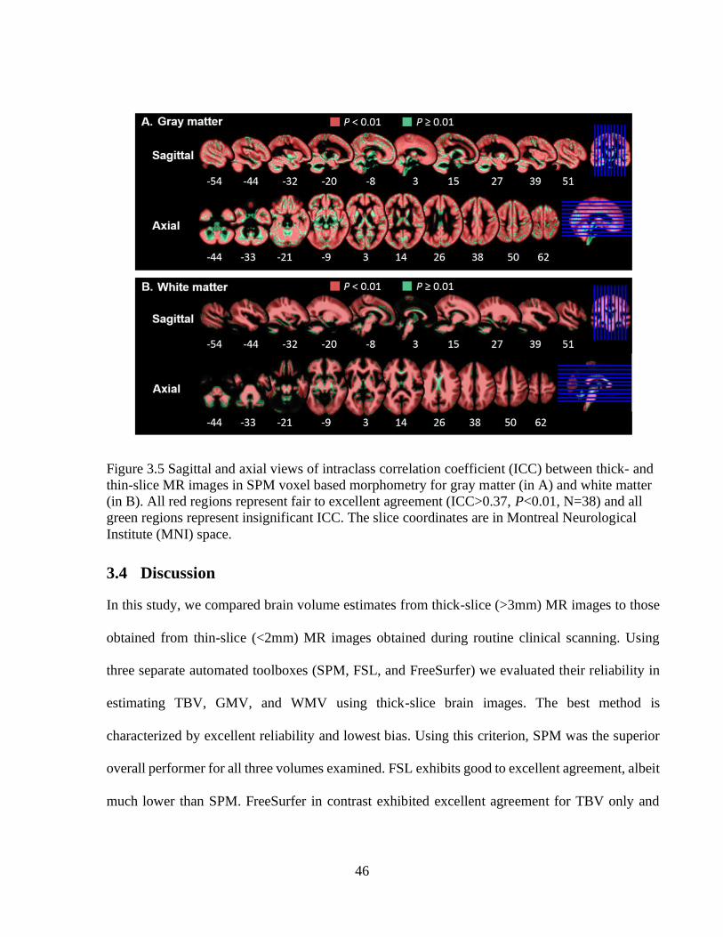
46
Figure 3.5 Sagittal and axial views of intraclass correlation coefficient (ICC) between thick- and
thin-slice MR images in SPM voxel based morphometry for gray matter (in A) and white matter
(in B). All red regions represent fair to excellent agreement (ICC>0.37, P<0.01, N=38) and all
green regions represent insignificant ICC. The slice coordinates are in Montreal Neurological
Institute (MNI) space.
3.4 Discussion
In this study, we compared brain volume estimates from thick-slice (>3mm) MR images to those
obtained from thin-slice (<2mm) MR images obtained during routine clinical scanning. Using
three separate automated toolboxes (SPM, FSL, and FreeSurfer) we evaluated their reliability in
estimating TBV, GMV, and WMV using thick-slice brain images. The best method is
characterized by excellent reliability and lowest bias. Using this criterion, SPM was the superior
overall performer for all three volumes examined. FSL exhibits good to excellent agreement, albeit
much lower than SPM. FreeSurfer in contrast exhibited excellent agreement for TBV only and

47
poor agreement for GMV and WMV. In VBM using SPM12, our results indicate fair to excellent
reliability between thick- and thin-slice images for GM and WM maps for the majority of brain
voxels. Our findings suggest that thick-slice MR images can be reliably used for estimating total
brain and brain tissue volumes using SPM, a widely applied automated method. Additionally,
clinical quality images may be utilized for VBM in SPM.
Previous work has not directly attempted to compare thick- and thin-slice MR image reliability
for computing brain volumes although several studies have examined the effect of sparse sampling
of MR image slices for computing TIV manually (Eritaia et al., 2000; Sargolzaei et al., 2014).
These studies indicated that sparse sampling can provide accurate TIV estimates. Similarly, our
findings indicate that thick-slice images can provide reliable brain volume estimates using
automated methods. Previous studies indicate that SPM gives the most accurate estimates for brain
volumes in comparison to ground truth (Klauschen et al., 2009; Malone et al., 2015). Our study
builds on these findings and we report that SPM gives the most reliable estimates for TBV, GMV,
and WMV among the three methods when utilizing thick-slice images.
In addition, we demonstrated that the reliability of automated methods for thin vs thick
estimation for TBV was stable with increasing age but declined marginally for GMV and WMV.
Although there was a marginal decline of ICC for GMV and WMV, all ICC values remained
excellent. The decline in GMV and WMV reliability can be attributed to decreasing GM and WM
contrast with age (Kim et al., 2002; Knight et al., 2016).
There are two important limitations to address regarding our findings. First, images were
acquired from different scanners and had varying acquisition planes and acquisition sequences.
Despite this heterogeneity, consistent results emerged. We therefore do not expect that differences

48
in scanners and scanner parameters significantly influenced the results. The second limitation is
that our study has a small sample size and our findings need to be further validated using a large
dataset.
Despite the presence of large archives of clinical quality MR images this source of valuable
data has not been utilized to its full extent in research studies. This study demonstrates the potential
to utilize large existing clinical brain imaging archives for radiomics opening a vast new data
resource to researchers and clinicians for a variety of studies. These include clinical
outcome/association studies, studies of pharmacologic efficacy, and phenome/genome-wide
association studies.
49
Chapter 4
4 CTSeg: A Probabilistic brain segmentation method
for clinical quality head CT images.
4.1 Introduction
Total brain volume (TBV) is an important measure for assessing brain atrophy in aging and
neurodegenerative diseases (Smeets et al., 2016). TBV is estimated from MR or X-ray CT brain
images by segmenting the brain parenchyma. A number of automated segmentation methods are
available for MR images that are extensively applied in the clinical domain (Giorgio and De
Stefano, 2013). In the clinical setting, CT is more widely used than MRI due to faster acquisition
speed, smaller number of contraindications, lower cost, and its ability to answer a range of clinical
questions (Li et al., 2016). In current practice, CT images are analyzed by visual inspection.
However, quantifying brain tissue volumes or brain volumetry is desirable for aiding accurate
diagnosis. Although a number of automated segmentation methods are available for MR images
that are extensively applied in the clinical domain (Giorgio and De Stefano, 2013), only a handful
of automated segmentation methods exist for head CT images. There are two major reasons
responsible for this limitation: CT images from healthy subjects are difficult and unethical to
obtain due to the permanent effects of the exposure to ionizing radiation as brain segmentation
methods are developed using healthy images for brain volumetry. Second, the contrast to noise

50
ratio in CT is low between various tissues (e.g. GM-WM contrast) making them undistinguishable
leading to the complexity in modelling them.
Several existing methods in CT segmentation are either semi-automated (Mandell et al.,
2015; Manniesing et al., 2017) targeted towards a specific brain region (Chen et al., 2009; Liu et
al., 2010; Ruttimann et al., 1993) or a disease condition (Cherukuri et al., 2018; Mandell et al.,
2015). Methods available for segmenting CT images for measuring global volumes metrics such
as TIV and TBV from images with no detectable pathology were not formally validated (Gupta et
al., 2010; Imabayashi et al., 2013; Kemmling et al., 2012). Some well validated methods segment
only TIV (Aguilar et al., 2015; Muschelli et al., 2015) but not TBV. However, TBV is more
indicative of disease conditions in neurodegenerative diseases (Jenkins et al., 2000) and TIV is
used merely as a nuisance variable for normalization purposes. Manniesing et al., (2017) estimated
TBV using head CT, but used enhanced CT images. However, their method cannot be applied to
single time point CT images with no image enhancement. Irimia et al., (2019) adapted SPM12
(http://www.fil.ion.ucl.ac.uk/spm/) (Ashburner and Friston, 2005), a widely used MRI based
segmentation method, for CT segmentation and validated by comparing with MRI images
segmented using Freesurfer. However, they validated only the accuracy of ventricular CSF and
not TIV or TBV.
We present a fully automated CT segmentation (CTSeg) algorithm for brain segmentation and
estimation of TBV and TIV from non-enhanced single time-point head CT images by adapting
SPM12. CTSeg was validated for brain segmentation and volume estimation by comparing with
manual segmentation (N=20). Additionally, we present a clinical application where CTSeg is used

51
to show TBV differences in AD (N=116). Sections in this chapter are taken from our article
published in the American Journal of Neuroradiology as Adduru et al., (2020)
4.2 Materials and Methods
4.2.1 Study population
This study was reviewed and approved by Geisinger’s Health System Foundation’s institutional
review board. No protected health information (PHI) was collected or accessed for the subjects
used in this study. This study was a part of a larger research initiative on the question of leveraging
clinical imaging archives for research studies. A large cohort of 10000 patients containing head
CT scans were identified from Geisinger health system’s clinical picture archiving and
communication system (PACS). The patients who have undergone CT scans were selected by
going back in time, starting from March 2014, until a count of 10000 patients was reached. The
oldest scan was from September 2007. All the scans were fully de-identified.
From the cohort we created two datasets: (1) manual segmentation dataset (N=20, subjects free
of brain abnormalities) and (2) AD dataset (N=167, subjects with and without a diagnosis of AD).
Fifteen of the AD subjects had catheters and were removed from further analysis. The AD dataset
that was further analyzed consisted of 152 subjects.
4.2.2 Manual segmentation dataset
A total of 20 subjects (mean age, 66 years; age range, 32-89 years; 10 females) were randomly
selected for manual segmentation of the intracranial space and the brain parenchyma. These
subjects were free of brain abnormalities and were unremarkable according to the radiology

52
reports. Additionally, through visual inspection we confirmed that the images were free of imaging
artifacts.
4.2.3 AD dataset
The initial cross-sectional AD dataset consisted of 62 subjects (mean age, 77 years; age range, 68-
83 years; 41 females) with a diagnosis of AD and 90 controls (mean age, 78 years; age range, 68-
83 years, 64 females), who did not have a diagnosis of AD or dementia. AD and control subjects
were selected based on ICD 9 (ICD-9-CM 331.0) codes (“ICD – Classification of Diseases,
Functioning, and Disability (2009) National Center for Health Statistics,” n.d.). Subjects
containing gross head pathologies visible on CT images were excluded from this study. All CT
images were free of imaging artifacts and the radiology reports of the images confirmed no acute
pathologies or brain abnormalities. A retrospective evaluation indicated that the controls obtained
a CT scan following headaches or head injury. The CT images were acquired using multiple CT
scanners and details of the scanner models and image parameters are provided inTable 4.1.

53
Table 4.1 Image and Scanner parameters
Manual segmentation
Dataset (N=20)
AD Dataset (N=152)
AD (N=62) Controls (N=90)
Scanner Model
GE LightSpeed VCT (12)
GE LightSpeed16 (4)
Toshiba Aquilion (4)
GE LightSpeed VCT (26)
GE LightSpeed16 (18)
Siemens Sensation 64 (1)
Toshiba Aquilion (17)
GE LightSpeed VCT (42)
GE LightSpeed16 (19)
Siemens Sensation 64 (1)
Siemens Sensation 16 (2)
Toshiba Aquilion (26)
Slice Thickness
(mm)
5.0 5.0 5.0
Pixel size
(mm)
0.4x0.4 (2)
0.5x0.5 (18)
0.4x0.4 (5)
0.5x0.5 (57)
0.4x0.4 (3)
0.5x0.5 (87)
Note— Number of images are indicated within the parenthesis.
4.3 Image Pre-processing
The DICOM images obtained for above selected subjects from the PACS archive were converted
to NifTi format using dcm2niix software (provided with MRIcroGL, 2016 version) (Li et al.,
2016). During the conversion dcm2niix automatically corrected the images for both gantry tilt, and
varying slice thickness within the image. All the images were reconstructed with 5mm slice
thickness.
4.3.1 Manual Segmentation
Manual segmentation was performed by a trained operator using the ITK-SNAP 3.6
(www.itksnap.org) (Yushkevich et al., 2006). The intracranial space was outlined according to the

54
guidelines provided by (Nordenskjöld et al., 2013). The segmented intracranial image was then
used to segment the brain parenchyma by tracing the boundary between brain tissue and CSF.
4.3.2 Automated brain segmentation
CTSeg adapts the unified segmentation algorithm from the statistical parametric mapping (SPM)
toolbox, version 12 (http://www.fil.ion.ucl.ac.uk/spm/software/spm12/). SPM is widely used for
segmenting brain tissues such as the GM, WM, CSF, and skull from MR images. SPM creates
probabilistic tissue maps for each tissue type, and these maps describe the probability of each voxel
belonging to a certain tissue. SPM segments the brain tissues by iteratively modeling the intensity
distribution of each tissue type to derive posterior tissue probabilities using Bayes rule followed
by spatial normalization of the standard tissue probabilistic atlas maps (TPM) (Mazziotta et al.,
2001) to the obtained posterior probabilistic map, and updates the priors to be used in the next
iteration. This method is independent of the absolute tissue intensity in the original image, i.e., the
intensity distributions are modeled for each image independently, which makes this method easily
adaptable for segmentation of brain images from different modalities that have different intensities
for the tissues. CT images differ from MR images in both, the range of tissue-intensity, and the
contrast-to-noise ratio between tissue types. In this work, we adapt SPM segmentation to model
CT image intensities.
The first step in SPM segmentation is to perform an initial registration of the native space MR
image to be segmented onto an International Consortium of Brain Mapping (ICBM) MR brain
template (Mazziotta et al., 2001) in the MNI space. The registered image iteratively goes through
tissue classification, bias-correction, and spatial normalization until all the parameters are
optimized to construct the final partial tissue volume maps (Ashburner and Friston, 2005). The

55
initial registration of native space image is the only step that is specific to an MR image as the
template used is an MR template. We adapted this method for our CTSeg pipeline to perform CT
image segmentation by using a CT template, that was registered to the TPM or the ICBM MR
template, needed for the initial affine registration step. Using an adult CT brain template developed
by Rorden et al., (2012), we aligned the CT image to TPM in the MNI space. In the process of
creating the CT template, they used an intensity transformation for the CT images for better
registration with the MR image template. The CT template thus created was in the new intensity
space and therefore an initial step was required to transform the CT image intensities before
proceeding with the registration. The TPM used here during segmentation was created originally
for MR images. However, TPM only contains voxel wise tissue probabilities and is independent
of the imaging modality. Therefore, we used the default TPM provided in SPM for the CTSeg
pipeline.
Figure 4.1 CTSeg pipeline for intracranial space and brain parenchyma segmentation from head
CT images. Within parenthesis is the 3D coordinate space of the image. MNI: Montreal
Neurological Institute.

56
The CTSeg pipeline is outlined in Figure 4.1 and the steps involved in the pipeline are
described below:
1. Intensity transformation: CT image voxel intensities (in Hounsfield units (HU)) are
transformed to the Cormack units using the method outlined in Rorden et al., (2012) to
match the intensity space of the CT template.
2. Registration: The transformed image is then spatially registered to the CT template
using a 12-parameter affine registration using FMRIB image registration tool (FLIRT)
(Jenkinson et al., 2002a; Smith et al., 2002). The affine matrix obtained during the
registration is retained for use in Step 5.
3. SPM segmentation: The registered CT image is segmented using SPM, with default
parameters, to create tissue probability maps for GM, WM and CSF. The affine
regularization option is selected as ‘no affine registration’ as we already registered the
CT image to the MNI space template in Step 2.
4. Adding probabilistic maps: GM and WM maps are added to obtain a probabilistic map
for the brain parenchyma and GM, WM and CSF maps are added to obtain the
probabilistic map of the intracranial space.
5. Affine transformation to native space: The probabilistic segmentation maps of the brain
and intracranial space are transformed back to the native space of the original CT image
using the inverse of the affine registration matrix computed in Step 2.

57
6. Binarization: The probabilistic maps of the intracranial space and brain parenchyma in
the native space are binarized by thresholding using respective optimal threshold values
to create binary segmentation maps. Selection of optimal threshold is discussed in the
next section.
Though CTSeg creates individual GM and WM maps we summed them up to obtain brain
parenchymal maps to obtain TBV. Moreover, the validity of individual GM and WM maps derived
through the above process is questionable due to low contrast to noise ratio between the tissues in
CT. Though several previous studies used GM and WM probabilistic maps obtained from CT
images (Imabayashi et al., 2013; Kemmling et al., 2012), they did not systematically establish the
validity of the GM and WM maps using ground truth segmentations.
OPTIMAL THRESHOLD SELECTION
The probabilistic maps of the brain and the intracranial space obtained by applying CTSeg were
binarized by thresholding them to obtain the respective binary masks and were compared with
their respective manual segmentation masks using Dice similarity index (DSI) (Dice, 1945). DSI
was calculated using the following formula:
𝑆𝐼 =2 × 𝑇𝑃
2 × 𝑇𝑃 + 𝐹𝑁 + 𝐹𝑃
where 𝑇𝑃 refers to the ‘True Positive’ voxels where both the binary mask voxels and the
corresponding ground truth voxels (from manual segmentation) indicated the tissue presence. FP
refers to ‘False Positive’ voxels where the binary mask indicated the tissue presence when there
was no tissue in ground truth. FN refers to the number of ‘False Negative’ voxels where the binary
mask indicated no tissue while the ground truth indicated tissue presence. For both brain and
58
intracranial probabilistic maps, DSI was computed for a range of probability threshold values
between 0 and 1 on the training dataset (subset of manual dataset) and tested on the rest of the
images. The optimal threshold was selected using the following procedure for brain and
intracranial space maps independently: A set of 10 images from the manual dataset were randomly
selected as the training set with the remaining 10 used for testing. All the voxels from images in
the training set were pooled into a single array, separately for the probabilistic map and the manual
segmentation mask. The optimal threshold was identified using random search between 0 and 1
as the threshold value that exhibits the highest DSI on the pooled array of voxels. The optimal
threshold was then applied to binarize the probabilistic maps of the test images and DSI was
computed for each test image individually. The robustness of the optimal thresholds was also
verified using leave-one-out cross-validation.
4.3.3 Statistical Methods
The overlap between the automated and manual segmentation masks was measured using Dice
similarity index (DSI) (Dice, 1945). TIV and TBV were obtained from the probabilistic maps as
well as the binary masks obtained using CTSeg. For probabilistic maps, volumes were calculated
by integrating the partial tissue volumes (tissue probability × voxel volume) over all the voxels
from the respective tissue maps. Volume estimates were calculated from binary masks, by
multiplying the number of masked voxels by the unit voxel volume.
Volumes estimated using CTSeg were compared with the manual estimates using scatter plots
and Pearson’s correlation coefficient. The systematic bias was assessed using Bland-Altman (B-
A) analysis (Martin Bland and Altman, 1986) and percentage difference calculated as a percentage
of the manual estimates. The absolute agreement between automated and manual volumes was

59
evaluated using the intra-class correlation coefficient (ICC) computed using two-way ANOVA
(McGraw and Wong, 1996) with fixed effects. The volumes were checked for normality using the
Kolmogorov-Smirnov test (Massey, 1951).
The TIV estimates of CTSeg were also compared with the state-of-the-art brain extraction
method (BET) for CT (Muschelli et al., 2015). The images were processed using the BET pipeline
with the smoothing option. The bash script used for this pipeline is available at
http://bit.ly/CTBET_BASH. The TIV was estimated by integrating the volumes of the voxels from
the binary intracranial mask.
CTSeg estimated volumes from the images of age-matched AD and control subjects were used
to compare brain atrophy between AD and controls. AD and control subjects were age-matched
by minimizing the age-difference using the MatchIt package (Ho et al., 2011) in R (Core Team,
2013). Previous studies have demonstrated that sex has no significant effect on TBV as a
percentage of TIV (%TBV) (Smith et al., 2007) as it is a normalized measure that accounts for the
variability introduced by the head size and sex (Kruggel, 2006; Smith et al., 2007). Therefore,
subjects were not sex-matched as all our analyses were performed on %TBV. TBV vs TIV, and
%TBV vs age scatter plots were used to compare brain atrophy in AD and controls. Linear
regression models were used to determine the significance of age, sex and ADdiagnosis on %TBV.
For the regression models, age x ADdiagnosis interaction term was added to check if the rate of
brain volume loss was significantly different between AD and controls. Additionally, we
investigated the effect of TIV by modeling TBV using TIV as a confounding factor in the linear
models, as recommended in recent studies (Nordenskjöld et al., 2013; Voevodskaya, 2014). TIV
and sex were in addition to age and ADdiagnosis while modeling TBV. Results with P < 0.05 are

60
considered significant for all statistical analyses. Statistical analyses were performed using Python
2.7, R 3.4.3 and MATLAB 8.6.0.
4.4 Results
4.4.1 Segmentation
CTSeg successfully segmented all 20 images from the manual segmentation dataset. The optimal
image intensity threshold obtained using a random selection of 10 training images was 0.2 for the
brain mask and 0.0006 for the intracranial mask. These thresholds were robust when applied on
the test set (Figure 4.2).
Figure 4.2 Dice similarity index (DSI) computed for brain and intracranial binary masks of the
test subjects.

61
Binary masks from CTSeg agreed well with that of the manual segmentation masks (DSI was
0.94±0.008 for brain, and 0.98 ± 0.002 for the intracranial masks). The gyri and sulci in the superior
slices of the brain were well captured by CTSeg (Figure 4.3).

62
Figure 4.3 Axial views of head CT image slices for the three subjects that showed highest TBV
error. Top row of each subject is the original CT image viewed in brain intensity window (40-80
Hounsfield Units) and second row is the binary brain mask of CTSeg overlaid on top of manual
segmentation mask and the original CT image slices. Brown represents regions where CTSeg
and the manual segmentations agree. Red regions represent false positive labelling by CTSeg and
green regions represent the false negatives.

63
Figure 4.4 Axial views of head CT images for the three subjects that showed the highest TIV
error. Top row of each subjects is the original CT image viewed in bone intensity window (300-
1500 Hounsfield Units) and second row is the binary intracranial mask from CTSeg overlaid on
top of manual segmentation mask and the original CT image. Brown regions represent the voxels
where the CTSeg and manual segmentations agree. Red regions represent false positive labelling
by CTSeg and green regions represent the false negatives.

64
4.4.2 Brain volumetry
Comparison between automated and manual volume estimates is presented in Table 4.2. The
binarized TBV, and TIV estimates showed excellent agreement with the manual estimates (ICCs
were 0.94 and 0.97 respectively) whereas the probabilistic estimates showed lower agreement
(ICCs were 0.74 and 0.71 for TBV and TIV respectively). The variance of ICC was low for
binarized estimates. TIV estimated using BET also showed excellent agreement with manual (ICC,
0.94) but lower than binarized TIV from CTSeg. Binarized CTSeg also exhibited the lowest bias
in-terms of the percentage difference (Table 4.2) in the B-A plots (Figure 4.5) for both, TIV (mean
difference of -0.04L for CTSeg binarized vs. -0.05L for BET and -0.13 for CTSeg probabilistic)
and TBV(mean difference of 0.02L for CTSeg binarized vs. -0.08L for CTSeg probabilistic for
TBV). The pattern of the linear fit in the B-A plots shows that error increases with average volume
and therefore head size, for both TIV and TBV estimates from CTSeg. However, the rate of
increase is higher for probabilistic estimates than binarized estimates of CTSeg. BET TIV estimate
showed lowest dependence of error on the average volume but showed larger bias than the
binarized CTSeg TIV. As the binarized CTSeg estimates showed better agreement with manual
estimates, proceeding evaluations are made only using the binarized CTSeg method.

65
Table 4.2 Comparison of automated TBV and TIV estimates with manual ground truth estimates.
Parameter Method %difference Pearson's r
(P-value)
ICC
(P-value)
Bootstrap
mean ICC
(95% CI)
TBV
CTSeg-
probabilistic
-7.22±2.98 0.96
(<1E-10)
0.74
(<1E-10)
0.727
(0.724, 0.730)
CTSeg-
binarized
1.58±3.46 0.95
(<1E-10)
0.94
(<1E-10)
0.937
(0.935, 0.939)
TIV
CTSeg-
probabilistic
-12.15±1.44 0.99
(<1E-20)
0.71
(0)
0.685
(0.680, 0.689)
CTSeg-
binarized
-3.28±1.36 0.99
(<1E-20)
0.97
(0)
0.962
(0.961, 0.963)
BET -5.12±0.667 0.99
(<1E-25)
0.94
(0)
0.930
(0.928, 0.932)
Note: %difference is reported as mean ± standard deviation.

66
Figure 4.5 (Top row) Scatter plots of automated vs manual volume estimates. Thin black line
represents the line of equality. Thick black lines represent the linear fit between automated and
manual volumes. (Bottom row) Bland-Altman plots presenting automated minus manual volumes
on y-axis and average of automated and manual volumes on x-axis. Mean difference and ± 2
standard deviations (σ) are represented by dotted and dashed horizontal lines respectively
4.4.3 Brain volumetry in AD
CTSeg was applied to the AD dataset containing 152 images. CTSeg successfully segmented 135
images (58 AD and 77 controls) of 152 images (88%). Reasons for CTSeg failures are discussed
in the section 4.4.4. After excluding CTSeg failures, 58 control subjects were optimally age-
matched to 58 AD subjects. A paired t-test confirmed no significant age-difference (P=0.74)
between the two groups after age-matching. Group comparisons were performed on binarized
volumes estimated from the age-matched subjects. TBV and %TBV computed for AD and controls
are presented in Figure 4.6.

67
Figure 4.6 (left) Scatter plot of %TBV estimated using CTSeg maps vs age. (right) Scatter plot of
TBV vs TIV. Lines represent linear fits.
Linear fit to %TBV indicates a higher loss with age in the AD group than controls. We
observed significantly lower mean %TBV (P<0.05) in the AD group (76.24±2.87) than the control
group (77.52±3.05). A paired t-test between %TBVs of the matched subjects also showed a
significant difference (P<0.05) between the two groups. The linear fit in the TBV vs TIV plot
shows that the slope is lower for AD suggesting lower TBV to TIV ratio in AD subjects.
Linear regression analysis (Table 4.3) showed that both age (P<0.001) and ADdiagnosis
(P<0.05) had significant effect on %TBV. Age x ADdiagnosis term was insignificant as an
interaction term in the linear model. Similar results were observed when TBV was modeled using
sex and TIV as additional covariates. Age and ADdiagnosis exhibited significance when these
variables are modeled as main effects. TIV exhibited significant contribution in all regression
models. Results remained same when sex was removed from the main effects model.
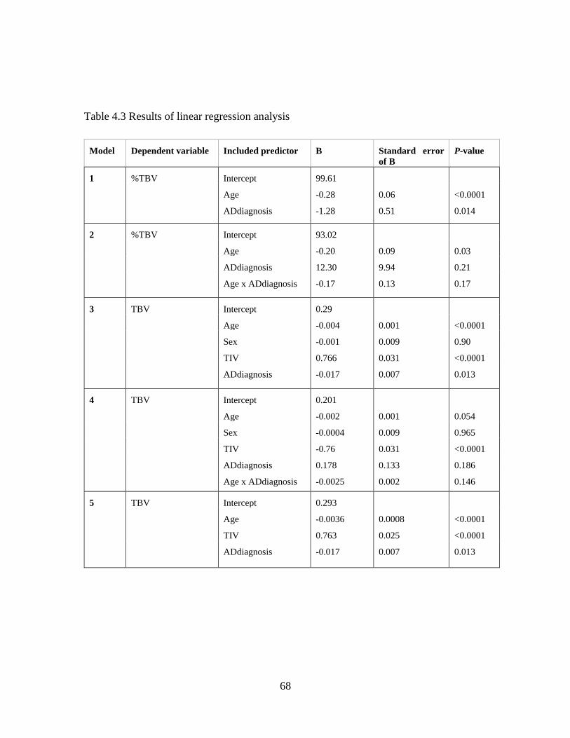
68
Table 4.3 Results of linear regression analysis
Model Dependent variable Included predictor B Standard error
of B
P-value
1 %TBV Intercept 99.61
Age -0.28 0.06 <0.0001
ADdiagnosis -1.28 0.51 0.014
2 %TBV Intercept 93.02
Age -0.20 0.09 0.03
ADdiagnosis 12.30 9.94 0.21
Age x ADdiagnosis -0.17 0.13 0.17
3 TBV Intercept 0.29
Age -0.004 0.001 <0.0001
Sex -0.001 0.009 0.90
TIV 0.766 0.031 <0.0001
ADdiagnosis -0.017 0.007 0.013
4 TBV Intercept 0.201
Age -0.002 0.001 0.054
Sex -0.0004 0.009 0.965
TIV -0.76 0.031 <0.0001
ADdiagnosis 0.178 0.133 0.186
Age x ADdiagnosis -0.0025 0.002 0.146
5 TBV Intercept 0.293
Age -0.0036 0.0008 <0.0001
TIV 0.763 0.025 <0.0001
ADdiagnosis -0.017 0.007 0.013

69
4.4.4 Segmentation failures in AD dataset
CTSeg failed to produce acceptable segmentations for 4 of 62 AD images and 13 of 90 control
images. Failures in the segmentation include segmentations of non-brain regions like eyes as brain
tissue or segmentation maps that do not resemble brain or intracranial space. Table 4.4 summarizes
the failure rate of the CTSeg for different scanners. Overall the failure rate was <15% across all
the scanners.
Table 4.4 Segmentation failure rates of CTSeg pipeline for different scanners.
Scanner AD controls Total
GE LightSpeed VCT 2/26 7/42 9/68 (13%)
GE LightSpeed16 1/18 3/19 4/37 (11%)
Siemens Sensation 16 0/0 0/1 0/1 (0%)
Siemens Sensation 64 0/1 0/2 0/3 (0%)
Toshiba Aquilion 1/17 3/26 4/43 (10%)
Total 4/62 (6%) 13/90 (14%) 17/152 (11%)
Note—Values are 𝑁𝑓𝑎𝑖𝑙𝑒𝑑/𝑁𝑡𝑜𝑡𝑎𝑙, in parenthesis are failure rates as a percentage.
4.5 Discussion
TBV is an important measure for assessing brain atrophy in AD and other
neurodegenerative diseases. Although CT is widely used in the clinical setting, segmentation
methods to estimate TBV from head CT images are not available. We presented CTSeg, an
automated head CT segmentation method and validated the method by comparing with manual
segmentation.

70
TBV and TIV from binary CTSeg masks showed better agreement with manual estimates
than the TBV and TIV estimates from probabilistic masks. This was expected as the MRI based
default TPM that we used does not model some of the anatomy present in CT images and
binarizing the masks by thresholding mitigated these errors. Additionally, the systematic bias in
TIV estimate using the binary masks was better than TIV estimated using a BET based method by
Muschelli et al., (2015).
The utility of CTSeg was demonstrated in a cross-sectional dataset containing AD and
control groups. We found that CTSeg estimated volumes exhibited significant %TBV (P<0.05)
difference between AD and control groups in a linear regression model with age, sex and
ADdiagnosis as covariates. The sex of the subjects had no significant effect on the %TBV. This
finding is in agreement with previous findings using MR images that normalized global brain
volumes using TIV (Kruggel, 2006; Smith et al., 2007). The average %TBV estimated from AD
images was lower than that for matched controls. The statistical insignificance of age x
ADdiagnosis interaction on %TBV can be attributed to the cross-sectional nature of our dataset.
We expect that significant TBV group differences can be achieved if longitudinal head CT images
of the same subjects are tracked. Further, some of the %TBV variability may be due to not
accounting for the duration from the actual onset of AD with respect to the time of CT image
acquisition. Another factor that may have contributed to the %TBV is that our controls may have
atrophy due to undiagnosed disorders. We expect to see higher AD differences if compared against
healthy controls. Additionally, when TBV is modeled with TIV as a confounding variable we
observed similar results as with %TBV. TIV was a significant confounding variable in all the
models. Sex was insignificant in all the models suggesting that correction for TIV removes the

71
structural differences between males and females, which agrees with previous findings using MRI
estimated volumes (Voevodskaya, 2014).
Unlike MRI, the intensity of CT images is standardized and is a measure of radiation
attenuation of the tissue. Therefore, we do not expect the scanner variability to have significantly
affected our method. The standardized intensity in CT is, in fact, an advantage and makes the
comparison of CT images across scanners easier, compared to MR images. Additionally, we
expect the optimal thresholds of CTSeg to be widely applicable as SPM models the tissue
intensities separately for each image. We confirmed the optimal threshold using two different
approaches: random search and leave-one-out cross-validation. High DSI in both approaches
demonstrated the robustness of the optimal threshold. However, further validation on a larger
dataset is required to verify the robustness of the threshold at different noise levels of CT images.
In CTSeg we used a standard MR image based TPM specific to an age range of 18-90 years
for the segmentation (Mazziotta et al., 2001). The CT template used for initial registration was
developed for an age range of 46-79 years (Rorden et al., 2012). Although the age of the subjects
used for this study is 67-89 years, we achieved a good segmentation accuracy using the standard
TPM and the CT template. However, if age appropriate CT-based TPMs are used, we expect that
segmentation accuracy can further improve. The TPM and the CT templates were created using
images without brain abnormalities. Therefore, CTSeg assumes that the CT images to be
segmented have brains that are free of large structural abnormalities like glioma, stroke, surgeries,
and of image artifacts due to beam hardening and implants. CTSeg can be extended for applications
for abnormal brain, like identifying lesions (Cabezas et al., 2011).

72
CTSeg marginally overestimated TBV due to the misclassification of dura as brain, in the
superior slices of the image. This can be attributed to the low contrast-to-noise ratio between the
soft tissues of CT images. Misclassification of dura is a known problem even in the segmentation
of T1 weighted MR images (Viviani et al., 2017). TIV and TBV estimates from all automated
methods tested in this study exhibited a linear dependence of error with head size. Binarizing the
probabilistic maps using an optimal threshold slightly reduced this linear dependence to some
extent and this phenomenon can be attributed to several reasons. One reason may be partial volume
effect, where a single voxel represents two or more tissues due to the finite spatial resolution of
the image (Tohka et al., 2004). The number of voxels at tissue boundaries increases with head size
thereby increasing the error in volume estimation due to the partial volume effect. The linear
dependence of error and head size can also be attributed to errors in spatial registration and
allometric effect of the tissue priors. In the case of intracranial mask, the optimal threshold was
very low due to the influence of the high bone intensity (compared to CSF) on the partial volume
effect for voxels near the bone-CSF interface.
We computed optimal thresholds for CT images with 5mm image slice thickness, which is the
clinical standard for CT images. As partial volume effect increases with slice thickness (Souza et
al., 2005) thresholds may need to be derived independently for images with different slice
thicknesses. However, it should be noted that CT images reconstructed with smaller slice
thicknesses exhibit a lower contrast-to-noise which can lead to larger errors in the segmentation of
brain tissue using CTSeg. Therefore, care should be taken when applying CTSeg to high-resolution
images. Upon close visual inspection, we note that some brain-CSF boundary regions were
misclassified especially in the left and right regions of the frontal lobe where the brain is closer to

73
the skull and in regions between the brain hemispheres where the dura is present (Figure 4.3). The
misclassifications in intracranial maps (Figure 4.4) were observed at the boundaries of the
intracranial space in the superior and inferior slices resulting in lower TIV estimates compared to
the manual. We also note that the binarized segmentation misclassified some parts of the eyes as
the intracranial space. This shortcoming can be corrected by registering a standard intracranial
mask on to the binary intracranial mask obtained using CTSeg and excluding the voxels classified
as TIV that are outside the registered standard intracranial mask (Malone et al., 2015).
4.6 Conclusions
We present CTSeg to automatically estimate TBV and TIV from non-enhanced head CT images
acquired for diagnostic purposes that were originally intended for visual evaluations by
radiologists. We show that CTSeg can accurately estimate TBV and TIV. Application of CTSeg
on CT images from AD and controls provides evidence that CTSeg can be used for detection and
tracking global brain atrophy in neurodegenerative diseases. AD does not exhibit symptoms until
the mild cognitive impairment stage which occurs several years after the onset and CTSeg may be
used to track brain atrophy in these patients. In addition, CTSeg can be applied to clinical CT
archives to develop normative brain volumes and to research studies involving neurodegenerative
diseases that exhibit global brain volume loss.
74
Chapter 5
5 Head CT segmentation using fully convolutional
neural networks with spatial context
5.1 Introduction
Currently available head CT methods are able to successfully estimate TIV but not TBV, the
volume of the brain parenchyma (Akkus et al., 2018; Muschelli et al., 2015). In our previous
chapter we developed CTSeg (Adduru et al., 2020), a method for segmenting head CT images to
segment brain parenchyma and intracranial space and accurately estimate both TBV and TIV.
CTSeg adapted SPM to segment the brain parenchyma and the intracranial space from CT images.
SPM being an atlas-based statistical modeling method, has the following limitations; poor
efficiency (takes ~20 minutes/image), requires age specific templates, poor performance when CT
images contain imaging artifacts or brain abnormalities. SPM is also sensitive to partial volume
effect which is prevalent especially in thick-slice standard of care CT images.
Convolution neural networks (CNN) have demonstrated state of the art performance in
segmenting brain MRI images (Akkus et al., 2017; Litjens et al., 2017). CNNs have been widely
adapted for medical image segmentation for tasks like whole brain segmentation (Moeskops et al.,
2016; Shakeri et al., 2016), tumor segmentation (Havaei et al., 2015; Menze et al., 2014; Shen and
Anderson, 2015), lesion segmentation (Brosch et al., 2016; Kamnitsas et al., 2017), and

75
hemorrhage segmentation (Kuo et al., 2019). CNNs are data-driven and they automatically learn
complex features when trained on a subset of data. Former CNN based segmentations provide
single label predictions for the complete input patch of an image (Ciresan and Giusti, 2013; Farabet
et al., 2013; Vaidya et al., 2015). These models have several limitations including slow prediction
times and post-processing (Bernal et al., 2018). These limitations are resolved by using fully
convolutional neural networks (FCNN) (Long and Shelhamer, 2015) that perform dense
prediction. FCNNs are different from traditional CNNs in their last layers where fully connected
layers are replaced by convolution layers containing filters of single pixel/voxel. Additionally,
FCNNs can perform segmentations on variable input sizes without change in performance while
enabling faster predictions (Kleesiek et al., 2016).
Ever since their introduction, FCNNs have been widely applied in semantic segmentation of
medical images. Newer FCNN architectures like Unet (Ronneberger et al., 2015) for 2D and Vnet
(Wangobani and Macdonald, 2016) for 3D improved the segmentation performance of the FCNNs
significantly and have demonstrated state of the art performance on various medical image
segmentation tasks (Zhou et al., 2019).
However, only a limited number of deep learning based methods are available, that were
properly validated for unenhanced head CT image segmentation. Among them are two methods
(Akkus et al., 2020; Kleesiek et al., 2016) for brain tissue segmentation for the purpose of brain
volumetry. However, both of these only segmented the intracranial volume and not the brain
parenchyma. Other available deep learning segmentation methods for head CT are for segmenting
specific brain abnormalities like hemorrhage (Helwan et al., 2018; Islam et al., 2019; Muelly and
Peng, 2019), tumors (Amiri et al., 2018; van der Heyden et al., 2019), or lesions (Gao and Qian,

76
2018). This lack of methods for CT brain segmentation can be attributed to the reasons that we
discussed in chapter 4, mainly to the unavailability of proper head CT image datasets. In the
context of brain segmentation Kleesiek et al. developed a 3D FCNN model to perform brain
segmentation on MRI images and showed state-of-the-art performance (Kleesiek et al., 2016).
Their approach included an additional post-processing step of using a connected component filter
to remove groups of connected voxels lying outside the skull. This additional step was required as
the CNNs are translation invariant (Rawat and Zenghui, 2017) and identify regions of same
patterns irrespective of the location. However, removing just connected components is not
sufficient as regions containing similar patterns may occur connected to the brain. For example,
regions inside the eye and optic nerve are connected to the brain and connected component filter
doesn’t filter such regions. Furthermore, this problem aggravates in the presence of noise
especially in case of the soft tissue regions in CT images. Therefore, a method of incorporating
location context into the FCNN is required to train the network to learn the spacial context.
In this work we present an FCNN architecture that incorporates location context to segment
brain and intracranial space from CT images. We train and validate our model on a dataset
containing 5mm non-enhanced standard of care CT images (N=20) by comparing with manual
segmentation. Additionally, we present a clinical application where the network is used to show
TBV differences in AD vs controls (N=116). To our knowledge this is the first application of a
deep learning network to segment head CT images.

77
5.2 Materials
5.2.1 Data
This work used head CT images obtained from the Geisinger Health system’s clinical imaging
archive. These images were originally collected for our previous study in chapter 4 and contain 20
CT images in the manual segmentation dataset and 152 images in the Alzheimer’s disease dataset.
The 20 CT images were manually segmented, and binary ground-truth tissue masks were created.
The AD dataset contained 62 AD subjects and 90 control subjects. For more information on the
subjects, image selection and manual segmentation please refer to Section 4.2.
5.2.2 Automated brain segmentation
FCNN
We used a 2D deep FCNN architecture that trains on 2D patches extracted from the axial slices of
the CT images. Model in Figure 5.1 (top) shows the architecture of the simple FCNN network for
CT segmentation. This network consists of seven hidden convolution layers followed by the final
1x1 convolution layer which is a softmax output layer that predicts the probabilities of each voxel
belonging to one of the following three tissue classes: brain, CSF and background. This network
was inspired by the architecture used to segment the intracranial space from 3D MRI (Kleesiek et
al., 2016). We experimented with several different variations of this architecture by
increasing/decreasing the number of layers and found negligible change in performance. However,
compared to their network, we used rectified linear unit (ReLu) as the nonlinear activation function
for all the hidden convolutional layers, a smaller input size of (61x61) and a larger filter size (7x7)
in the first layer followed by a 2x2 average pooling layer instead of max pooling for reasons as
explained below.

78
During training the network accepts a 61x61x1 2D input patch (corresponding to height, width
and channel respectively) from the CT image and applies the convolution operation with 16
different filters of size 7x7 in the first layer followed by the non-linear activation function
producing 16 2D features. The resulting features are down-sampled using an average pooling of
size 2x2. The average pooling acts as a low pass filter that filters the high frequency noise from
the 2D features. Since the signal to noise ratio in soft tissues is high for CT images the usage of
average pooling is advantageous as it filters out the noise from the features. The output of one
hidden layer is fed as an input to the next layer resulting in a final output of size 3x3 which is a
sparse output with a stride of 2x2 that covers an output field of 5x5.
FCNNs are capable of using variable input size patches (Bernal et al., 2018), e.g., an FCNN
trained on an input patch of size 61x61 can also be applied on a patch of different size e.g. 95x95.
However, the only requirement is that the resolution (mm/voxel) of both the patches are be similar.
This feature of FCNNs makes it faster to segment large images containing millions of voxels
compared to traditional CNNs that predict one voxel at a time.
FCNN WITH CONTEXT MASK (FCNN+CM)
One challenge when using CNNs is that the network is translation invariant. Which means that the
CNNs look for patterns in the image but are not sensitive to the spatial context on where the
patterns occur. If two regions, one inside the brain and the other outside the skull, have similar
intensity patterns the network may identify both the regions as brain. This leads to false positive
segmentations in locations outside the region of interest where similar intensity patterns occur.

79
Figure 5.1 Preprocessing pipeline for patch preparation and proposed network architectures. S1
and S2 are input image channels.
Neural networks can be trained to the learn the spatial context by using the location specific
features as inputs. This can be easily implemented in traditional single voxel prediction models by
supplying the dense layers with additional location specific input features (Ghafoorian et al., 2017)
e.g., the coordinates of the center voxel of the input patch. However, these location features are
very difficult to introduce in an FCNN model where the network only learns to recognize the
patterns but are incapable of learning the scalar values of the input features. Another possibility is
to create a model with multi-scale patches to train independent convolutional layers for each scale
like U-net (Ronneberger et al., 2015) or multi-scale fusion models. U-nets performed better
segmentation of complex structures, for example the subcortical brain structures, and multi-scale
fusion methods segmented white-matter hyperintensities. However, these complex architectures
lead to unnecessary increase in the number of parameters of the neural network, leading to model
overfitting.

80
Therefore, we used an approach in which we provide contextual information to the network
using a region mask to limit the search region where the network looks for important patterns only
within the mask. The contextual mask is provided as an additional channel along with the input
image patch. We create this mask by registering an MNI template to the CT image. First a CT
template defined in the MNI space is registered onto the CT image using a 12-parameter affine
matrix. This affine registration matrix is used to transform the ICBM 152 intracranial mask in the
MNI space (Fonov et al., 2009) onto the CT image. Figure 5.1 (bottom) illustrates the architecture
of our method.
5.2.3 Preprocessing:
Before creating patches for the network, the CT images were pre-processed using the following
steps:
1. Intensity transformation: CT image voxel intensities (in Hounsfield units (HU)) are
transformed to the Cormac units using the method outlined in (Rorden et al., 2012) to match
the intensity space of the CT template.
2. MNI ICV mask registration: CT template is registered onto the intensity transformed CT
image using a 12-parameter affine registration using FMRIB image registration tool
(FLIRT). This affine matrix obtained during the registration is used to register the ICBM
152 (Fonov et al., 2009) intracranial mask onto the CT image.
3. Intensity normalization: The CT image intensities are clipped to the [0-4500] range and
then rescaled to be within the [0-1] range. During clipping any intensity outside the
accepted range is set to the nearest boundary value of the clipping range.

81
TRAINING, VALIDATION AND TEST SETS
The manual segmentation dataset is randomly divided into 8 training, 4 development and 8 test
images.
PATCH PREPARATION
Patches of size 61x61 were extracted from each voxel neighborhood from each axial slice of the
CT images. For FCNN+CM model, 61x61 patches are extracted from the registered ICBM
intracranial mask and paired with corresponding image patches creating 61x61x2 patches. The last
dimension corresponds to the channel number.
5.2.4 Training
The neural networks were implemented in Python 3.5 using Keras 2.1.2 with tensorflow 1.4.1 as
the backend. Stochastic gradient descent algorithm with momentum of 0.9, and Nesterov (Bengio
et al., 2013) update was used to train the network weights to optimize a cross-entropy as the cost
function. We use a mini-batch size of 128. The weights were initialized randomly using the Glorot
initialization (Glorot and Bengio, 2010). To avoid overfitting, we used dropout regularization with
0.3 probability on all the hidden layers. At each step, batches of size 128 are created by randomly
sampling the patches without replacement from the training images. To increase the robustness of
the model, we modify the patch intensities by randomly shifting and scaling by a random value.
The intensities are shifted by adding a random value in the range [-0.15, 0.15] and scaled by
multiplying the patch intensities by a random value in the range [0.90, 1.10]. We initiate training
with a learning rate of 0.025 and reduce it to 0.001 after 200 epochs. Finally, we picked the best
model with the lowest error on the validation set.

82
5.3 Statistical Analysis
FCNN and FCNN+CM were used to segment and obtain the probabilistic masks of brain and CSF
from the manual segmentation dataset. The intracranial mask is obtained by adding the CSF and
brain masks. The probabilistic masks are binarized by classifying each voxel to the class with
maximum probability. The overlap between the automated and ground truth manual segmentation
masks was determined using Dice similarity index (DSI) (Dice, 1945). In addition, the sensitivity
score was also computed. As we perform a multiclass classification, sensitivity is computed in a
one vs all manner. For statistical significance a 5-fold cross validation is performed by training the
network on three folds of the data and using the other two folds for validation and testing. The
mean and standard deviation of the DSI of the test data are compared between the folds.
Additionally, the performance of FCNN based segmentation was compared with that of CTSeg .
TBV and TIV were estimated using the binary masks of the brain and intracranial space
respectively. Volumes were computed by multiplying the number of masked voxels in the binary
mask by the unit voxel volume. The estimated volumes from automated methods were compared
with the manual estimates using %difference, intra-class correlation (ICC) and paired t-test. A
two-way ANOVA (McGraw and Wong, 1996) with fixed effects was used to compute ICC. Bland-
Altman plots (Martin Bland and Altman, 1986) were used to assess the systematic bias in the
volumes obtained from the automated methods.
FCNN+CM and CTSeg were applied to estimate TIV and TBV from the images of age-
matched AD and control subjects. The estimated volumes were used to compare brain atrophy
between AD and controls. AD and control subjects were age-matched by minimizing the age-
difference using the MatchIt package (Ho et al., 2011) in R (Core Team, 2013). Previous studies

83
have demonstrated that sex has no significant effect on TBV as a percentage of TIV (%TBV) as it
is a normalized measure that accounts for the variability introduced by the head size and sex
(Kruggel, 2006; Smith et al., 2007). Therefore, subjects were not sex-matched as all our analyses
were performed on %TBV. TBV vs TIV, and %TBV vs age scatter plots were used to compare
brain atrophy in AD and controls. Linear regression models were used to determine the
significance of age, sex and ADdiagnosis on %TBV. For the regression model, age x AD diagnosis
interaction term was added to check if the rate of brain volume loss was significantly different
between AD and controls. A P-value < 0.05 is considered statistically significant for all the
analyses. All statistical analyses were performed using Python 3.5 using scikit-learn 0.19.1, and R
programming language.
5.4 Results
5.4.1 Segmentation
Table 5.1 presents the comparison of brain and intracranial space binary masks obtained using the
automated methods on the CT images from the test set (N=8). All three methods; FCNN,
FCNN+CM and CTSeg successfully segmented all the twenty manually segmented CT images.
We used the same thresholds for CTSeg (0.2 for brain, 0.0006 for intracranial mask) to binarize
the probabilistic masks as obtained in chapter 4. With highest DSI and sensitivity on the test set,
the FCNN+CM model (DSI: 0.953±0.005, sensitivity: 0.972±0.008) exhibited the best
segmentation performance among the three methods followed by FCNN which was only
marginally low. SPM exhibited lowest DSI and sensitivity. The above results were observed for
the validation and training images as well.

84
Table 5.1 Segmentation performance of automated methods using validation data
Brain ICV
DSI Sensitivity DSI Sensitivity
Test (N=8)
FCNN 0.951±0.006 0.971±0.007 0.985±0.004 0.986±0.008
FCNN+CM 0.953±0.005 0.972±0.008 0.989±0.003 0.988±0.007
CTSeg 0.942±0.006 0.945±0.009 0.977±0.003 0.962±0.007
Valid (N=4)
FCNN 0.942±0.010 0.967±0.010 0.985±0.003 0.985±0.005
FCNN+CM 0.946±0.009 0.967±0.009 0.989±0.003 0.988±0.003
CTSeg 0.930±0.013 0.958±0.004 0.979±0.001 0.968±0.003
Train (N=8)
FCNN 0.960±0.004 0.972±0.007 0.991±0.002 0.995±0.002
FCNN+CM 0.962±0.004 0.972±0.007 0.993±0.001 0.995±0.002
CTSeg 0.946±0.007 0.947±0.011 0.979±0.002 0.970±0.006
Note: Number of images are indicated within the parenthesis. Values are mean ± Standard deviation.

85
Figure 5.2 Axial views of head CT image slices for the two images for which FCNN+CM
showed highest TBV error. Binary brain mask of automated methods are overlaid on top of
manual segmentation mask and the original CT image slices. Yellow represents regions where
automated methods and the manual segmentations agree. Red regions represent false negative
labelling by the automated methods and green regions represent the false positives.
Brain masks obtained from FCNN+CM and FCNN matched the manual segmentation well
with low DSI for all of the subjects except the ones shown above. Both FCNN methods segmented
a region in the middle of ventricles as brain in both the subject images shown in Figure 5.2. When

86
images were examined retrospectively, we observed slightly higher intensity in those regions.
These regions may not be included in the manual segmentation due to human error. The images
show that the both the FCNN based methods were able to classify the dura correctly in the top
slices in both images shown in Figure 5.2. Whereas, SPM segmented dura as brain.

87
Figure 5.3 Axial views of head CT image slices for the two subjects for which FCNN+CM
showed highest TIV error. Binary Intracranial mask of automated methods are overlaid on top of
manual segmentation mask and the original CT image slices. Yellow represents regions where
automated methods and the manual segmentations agree. Red regions represent false positive
labelling by the automated methods and green regions represent the false negatives.

88
The segmentation masks of TIV from FCNN+CM and FCNN match well with that of the
manual segmentation (Figure 5.3). The FCNN methods were able to successfully segment the
boundaries of the CSF and skull regions despite the presence of the partial volume effect (Souza
et al., 2005) unlike CTSeg which was very sensitive to the partial volume effect and couldn’t
accurately segment the CSF-skull boundary which is illustrated by the presence of false positive
regions in the top slices of both the examples in Figure 5.3. The FCNN model segmented some
localized regions outside the skull as brain (Figure 5.3 B) whereas no such regions were found in
the segmentations of FCNN+CM supporting the value of using the context mask.
5.4.2 Brain volumetry
In this section the performance of the methods to compute brain volume metrics for TIV and TBV
is compared. Since FCNN+CM has exhibited that usage of contextual map has improved the
segmentation from the network variant without the contextual map, we will be comparing the brain
volume metrics between FCNN+CM and CTSeg from here on. Both the methods are compared
using the separate test set (N=8) from the manual segmentation dataset.

89
Table 5.2 Comparison of volume estimations using automated methods from test set (N=8).
% difference ICC ICC p-value Paired t-test
t-value
Paired t-test
p-value
TBV
FCNN+CM 3.92±2.77 0.89 <1E-4 4.30 <0.01
CTSeg -7.98±2.41 0.652 <1E-4 -8.69 <1E-4
TIV
FCNN+CM -0.09±1.16 0.99 <1E-6 -0.27 0.79
CTSeg -2.89±1.04 0.93 <1E-6 -7.12 <1E-3
Note: %difference values are mean ± standard deviation.
Figure 5.4 (left) Scatter plot of automated vs manual TBV estimates. (right) Bland-Altman plots
presenting difference between automated and manual TBV (y-axis) vs the mean of the automated
and manual TBV (x-axis). Solid, and dashed lines represent mean difference and 2 standard
deviations respectively.

90
Figure 5.5 (left) Scatter plot of automated vs manual TIV estimates. (right) Bland-Altman plots
present difference between automated and manual TIV (y-axis) vs the mean of the automated and
manual TIV (x-axis). Solid, and dashed lines are mean difference and 2 standard deviation
respectively.
Comparison between automated and manual volume estimates from the images in the test set
is presented in (Table 5.2). ICCs of TBV, and TIV estimates from FCNN+CM show excellent
agreement with the manual estimates compared to SPM. The paired t-test shows significant
difference between the estimated volumes and manual TBV for both the methods. However, the
statistical significance of FCNN+CM is higher than CTSeg. TIV estimates from FCNN+CM were
not significantly different from manual estimates, whereas the CTSeg estimates exhibited higher
difference. FCNN+CM also exhibited the lowest bias in-terms of the percentage difference (Table
5.2) and mean-difference in the B-A plots (Figure 5.4 and Figure 5.5) for both, TBV and TIV
estimates (0.04L and -0.09L respectively). The pattern of the linear fit in the B-A plots shows an
increase in error with average volume and therefore head size, for TBV. However, the rate of
increase for FCNN+CM is lower than for CTSeg. The TIV error dependence was very low for

91
FCNN+CM with a low systematic bias (mean-difference, 0.001L) whereas CTSeg showed a high
systematic bias (mean-difference, 0.045L).
5.4.3 Brain volumetry in AD
Figure 5.6 Brain volumes between AD and controls estimated using FCNN+CM (Top row) and
SPM (Bottom row). (left) Scatter plot of %TBV estimated using binarized CTSeg maps vs age
after excluding images with catheters. (right) Scatter plot of TBV vs TIV. Red and green represent
the AD, and the controls groups respectively. Solid lines represent linear fits.
FCNN+CM and CTSeg were applied to the AD dataset containing 152 images. CTSeg
successfully segmented 135 images (58 AD and 77 controls) of 152 images (88%). FCNN+CM

92
was able to successfully segment 148 (62 AD and 86 controls) of 152 images (97%). However, for
comparing the results between FCNN+CM and CTSeg we have only used same subjects that were
successfully segmented by CTSeg. After excluding the subjects that CTSeg failed to segment, 58
control subjects were optimally age-matched to 58 AD subjects. A paired t-test confirmed no
significant age-difference (P=0.86) between the two groups. TBV and %TBV of AD and controls
for both the methods are presented in Figure 5.6. The slopes of the linear fits to %TBV indicate a
higher loss with age in the AD group than in the controls. The linear fits are clearly separated in
case of FCNN+CM indicating that the AD subjects have lower brain volume than controls at all
ages. This trend is not observed for volumes estimated using CTSeg. The linear fit in the TBV vs
TIV plot shows that the slope is lower for AD suggesting lower TBV to TIV ratio in AD subjects
in FCNN+CM compared to CTSeg. The results of the statistical tests comparing %TBV between
AD and controls are presented in Table 5.3. We observe a significantly lower mean %TBV (P<1E-
6) in the AD group (72.64±3.45) than the control group (76.07±3.48) using FCNN+CM. A paired
t-test also confirmed a significant difference. Although a significant difference (P<0.005) was
observed between %TBV of AD and controls for CTSeg the difference was not as significant as
FCNN+CM. Linear regression analysis showed that both age and ADdiagnosis had significant
effect on %TBV for both the methods. This means that AD group exhibited lower %TBV than the
control group at all ages. However, these values had higher statistical significance in FCNN+CM.
Sex and age x ADdiagnosis variables did not exhibit any significant contribution to %TBV when
added as variables in the model for both FCNN+CM and SPM.

93
Table 5.3 Comparison of %TBV estimates between Alzheimer’s(N=58) and control subjects
(N=58).
%TBV
(AD)
%TBV
(Controls)
2 sample t-test
p-value
Paired t-test
p-value
Linear model p-values
age diagnosis
FCNN+CM 72.63±3.45 76.07±3.48 <1E-6 <1E-6 <1E-3 <1E-10
CTSeg 76.24±2.87 77.52±3.05 0.023 0.024 <1E-4 0.014
Note: -- % TBV values are mean ± standard deviation
5.5 Discussion
In this chapter we present FCNN+CM, a 2D deep FCNN with context masking, for the
segmentation of brain and intracranial volume from clinical quality 5mm thick-slice CT images.
We compare the performance of our network with FCNN, a similar network without context
masking, and SPM a state-of-the-art method adapted to perform CT segmentation. We compare
the segmentations of these two methods using DSI and sensitivity with manual segmented tissue
masks as the ground truth. ICC, %difference and paired t-test were used to compare the estimated
volumes. By comparing these metrics FCNN+CM was the best performer for both brain and ICV
estimation. Both TBV and TIV estimated using FCNN+CM exhibited excellent agreement with
manual volume estimates. The low dependence of volume error on the average TIV estimated
using FCNN+CM shows that the network is less sensitive to the partial volume effect in the voxels
near the CSF-skull boundary.

94
APPLICATION IN ALZHEIMER DATASET
The utility of FCNN+CM was demonstrated in a cross-sectional dataset containing AD and control
groups and was compared with the results from CTSeg. FCNN+CM estimated volumes exhibited
significant %TBV (P<1E-6) difference between AD and control groups at all ages. Linear
regression model also confirmed this result. The sex of the subjects had no significant effect on
the %TBV for both the methods. This finding is in agreement with findings from previous studies
using MR images that normalized global brain volumes using TIV (Voevodskaya, 2014). The
average %TBV estimated from AD images was significantly lower than matched controls for both
the methods. However, %TBV estimated using CTSeg was only marginally different between AD
and Controls. This can be attributed to over-estimation of TBV by CTSeg due to the inability to
segment regions like dura where the brain-dura boundary is affected by noise in CT. Furthermore,
CTSeg being an atlas-based method depends on the age specific atlas to perform accurate
segmentation. Usage of a healthy atlas to segment AD images may be one of the reasons for
inaccurate segmentation by CTSeg. FCNN+CM was robust and performed well in such difficult
to segment regions.
Compared to conventional brain segmentation methods which use hand crafted features, deep
learning models using CNN learn features in a data driven manner. However, deep learning
requires a training dataset that contains the required features, for the method to generalize well on
testing datasets. In brain tissue segmentation, brain images contain more or less similar imaging
features and the number of features that the network had to learn are small compared to general
domain image datasets that contains a variety of images. Therefore, our network needed only a
small set of images (N=8) for learning the task of segmenting brain and intracranial volume. Using

95
the 2D segmentation on each slice independently provided large number of image slices despite
the small number of 3D images. Additionally, usage of patches, and data augmentation, by adding
noise to the patches during training, further improved the model by making the model learn a
robust set of features. The requirement of small training dataset makes this network easy to train
and makes it easily adaptable to segment CT images of brain diseases, or images with artifacts etc.
This can be done by manually segmenting a small set of images and to train the network from
scratch or using transfer learning.
USE OF PATCH-BASED SEGMENTATION
Patch-based segmentation allows FCNN+CM to focus on a small portion of the image at a time
making the method robust to features like artifacts or abnormal brain conditions that may be
present elsewhere in the image. This allows the FCNN+CM to accurately segment regions that are
not affected by such artifacts. However, in Whole brain segmentation architectures, or atlas-based
methods like CTSeg, presence of the artifact in any part of the image effects the segmentation of
the entire image. This is because the atlas-based methods use registration of the image with the
atlas and registration is very sensitive to the presence of artifacts.
USAGE OF LARGE INITIAL FILTER SIZE
Large initial filter size (7x7) was beneficial as it learned to identify larger features that are required
for segmentation of simpler brain structures like brain parenchyma and intracranial volume instead
of learning unwanted smaller features responsible for more complex regions at the first layer.
Unlike MRI, such small features are dominated by noise in CT images and using smaller filter size
may learn on such noisy features thereby leading to overfitting. Usage of the average pooling layer
96
after the first convolutional layer helped to reduce noise present in the patch thereby improving
the signal to noise ratio of the larger structural features.
LOCATION CONTEXT CONTRIBUTION
Highest DSI for the FCNN+CM model show that the novel procedure in which contextual
information supplied as a second channel to the CNN was beneficial. The context information
provided in the form of an intracranial mask was successful in training the FCNN network to
distinguish if the classified voxels belonged to the background or the foreground (inside or outside
the cranium respectively).
INCORPORATION OF COORDINATES INSTEAD OF MASK
Previous methods to incorporate location information used coordinate information as additional
input features to the dense layers in the neural network architectures. However, single voxel
segmentation methods only segment one voxel at a time increasing the segmentation time
significantly. With FCNN+CM we have the advantage of incorporating location context as well
as making dense predictions. Furthermore, FCNN+CM can use larger input image-patches thereby
speeding up the segmentation unlike single voxel segmentation networks which use a fixed input
patch size.
We experimented with two types of rescaling; (1) rescaling the intensity transformed image
to [0,1] by using 0 as minimum intensity and maximum as the maximum intensity of the image
and (2) clipping the maximum intensity of the image to 4500 HU and using that as the upper bound
to rescale the image. The clipping method worked better, and the model was able to converge to a
lower validation loss. This is expected as the upper bound intensities are highly variable across CT
images. As all the high intensity voxels above 500HU are mostly bone, in CT, it is useful to clip

97
the images to a fixed higher bound for normalization so that the intensity distributions of various
tissues are normalized across images.
2D VS 3D
We used 2D convolution layers in the network that segment 2D patches obtained from the slices
of the CT images. Although 3D image data can provide more useful spatial information, given the
slice thickness of 5mm, image features present in consecutive slices were different. Furthermore,
use of 2D slices allows segmentation of CT images that do not contain the entire head, which is
often the case in diagnostic imaging, especially with CT where the usage is regulated due to the
ionizing radiation (Rorden et al., 2012).
RESTRICTED TO 5MM NOISE LEVEL CHANGES
One limitation of FCNN+CM is that the network cannot be used to segment slices with
significantly different resolution. This model was trained to segment CT images reconstructed with
5mm slice thickness and 0.4-0.5 mm/voxel resolution. Applying this model on images with
different resolutions will impact the prediction quality. However, by rescaling the input slices to
the same resolution will solve this limitation. Another solution is to train the network by feeding
small patches of the same image with different resolutions.
Unlike MRI, the intensity of CT images is standardized and is a measure of radiation
attenuation of the tissue. Therefore, we do not expect the scanner variability to have significantly
affected our method. Compared to MRimages, the standardized intensity in CT is, in fact, an
advantage and makes the comparison of CT images across scanners easier. However, further
validation on a larger dataset is required to verify the robustness of the method.

98
Before applying the trained network for segmenting CT images on new images from a different
scanner we recommend validating the performance of the network on a small set of images with
ground truth segmentations from that scanner. In case of a significant difference in performance,
the network should be retrained to adapt to the new image quality by applying transfer learning
using a small independent set of images acquired from the new scanner. Additionally, we advise
that the method may be calibrated from time to time using independently collected images that
represent the target population to ensure that the method exhibits acceptable performance.
MNI TIV MASK
We used a standard MNI space ICBM ICV mask specific to an age range of (47-88) to register to
the CT images. Although the images have ages different from that of the mask, we do not expect
this to influence the segmentation because of two reasons. First, we are only using an intracranial
mask which does not have age specific changes for the brain mask. Second, even if the registration
is not accurate, the neural network is capable of automatically learning these differences and can
incorporate these differences to segment the image.
5.6 Conclusion
In this chapter we present a 2D fully convolutional deep learning architecture FCNN+CM for
segmenting the brain and intracranial volume from 5mm standard of care head CT images. This
method incorporates spatial context using a standard space intracranial mask registered onto the
CT image and thereafter successfully segments regions within the mask to and achieve
segmentation with high accuracy. In addition to fast prediction times, FCNN+CM requires only a
few segmented ground truth labels and making it easy to adapt our method to a variety of head CT

99
images. Using a separate Alzheimer’s dataset, we also demonstrated the utility of this model to
automatically track brain atrophy in patients with AD. FCNN+CM also enables the inclusion of
clinical quality CT images in volumetric studies opening new data resources to researchers and
clinicians for variety of research studies.

100
Chapter 6
6 Conclusion
The main contributions in this thesis and their implication are discussed below. We first discuss
the major contributions and specifications of the studies. We will also briefly discuss future
directions and prospective studies on better understanding of methods for clinical quality images.
6.1 Contributions
6.1.1 Thick-slice clinical quality images are reliable for brain volumetry.
By comparing the performance of three widely used fully automated methods we demonstrated
that the thick-slice clinical quality brain MRI images can be reliably used for brain volumetry.
Global brain volume metrics like TBV, GMV and WMV can be reliably estimated using the
clinical quality images. This enables the inclusion of large clinical archives of brain images in
hospitals for a variety of clinical and research studies involving brain volume estimations.
6.1.2 SPM is the most reliable method for brain volumetry on clinical quality
images.
In chapter 3, in addition to finding the reliable usage of thick-slice images, we have shown that
SPM is the most reliable among the existing state-of-the-art MRI brain segmentation methods for
clinical quality images. Our image dataset was heterogeneous spanning different scanners and
image parameters. Despite the heterogeneity in the data, SPM exhibited consistent results.

101
However, our study used a small dataset and these results need to be further validated using a
larger dataset.
6.1.3 Clinical Quality images can be used for Voxel-based morphometry
We show that the clinical quality images can be reliably used for voxel-based morphometry except
for some regions at the boundaries of the brain tissues. This means clinical quality images can also
be used for group comparison studies enabling the inclusion of large imaging archives to study the
effect of diseases on various regions of the brain in comparison with healthy controls.
6.1.4 CTSeg is a reliable brain segmentation method for clinical quality head CT
images
In chapter 4 we presented a novel brain segmentation algorithm for clinical quality CT images by
adapting the reliable segmentation algorithm from our first study. We designed a pipeline using
the existing MRI segmentation algorithm for segmenting CT images and found that the brain
volume measurements were very accurate when validated by comparing with the measures derived
from ground-truth manual segmentations. With CTSeg, we then unlock a large clinical image
archive of CT images, much larger than that of the MRI. However, we had to binarize the
probabilistic maps as the bone intensity in CT was influencing the segmentation by a phenomenon
called partial volume effect. Several other disadvantages were observed in this approach due to the
very nature of the SPM algorithm. Being an atlas-based method, it needed age specific and group
specific atlases for accurate segmentation.

102
6.1.5 Clinical quality CT with CTSeg can be used for detection and tracking of brain
volume loss in AD.
We applied CTSeg on a large dataset containing images from AD and control subjects and found
that CTSeg derived volumes exhibited similar results as observed in previous studies with research
quality MRI images. This demonstrated that thick-slice clinical quality CT images can be used for
estimating and tracking brain atrophy in neurodegenerative diseases. However, a longitudinal
study is needed to further validate the method for tracking brain atrophy.
6.1.6 Deep learning brain segmentation method for CT surpassed the state-of-the
art in brain segmentation.
In chapter 5 we present a novel deep learning architecture to segment clinical CT images. This
method was trained on the same dataset that is used in the previous study. We used the ground
truth manual segmentations to train the deep learning architecture for segmenting the CT images
into brain and intracranial volumes. This method surpassed the performance of previous
segmentation methods for CT segmentation. The deep learning model was robust to data from
different scanners and also for images containing abnormal brain structures or artifacts. We used
normalization of the intensities before training and found that this improved the convergence of
the model significantly. One limitation of our model was that the model was trained for images
with a noise model in 5mm thick slice reconstructions of CT images. This means the model may
not be as robust when used on higher or lower resolution images. This may require retraining the
model using images with different resolutions. Additionally, we excluded images that contain
artifacts and abnormal brains as we do not have enough number of samples of those images to
train the deep learning model. However, with reasonable samples of image that exhibit artifacts
and other features, the deep learning based segmentation can be made more robust.

103
6.1.7 Contextual awareness helped deep learning brain segmentation network
Another contribution of this work is presenting a contextual aware neural network for
segmentation. Existing CNN based segmentation methods used only the sparse features derived
from the images. However, in images, same features repeat in different locations and the
classification of a region depends on the overall context in which these features have occurred.
Adding local features to the network in the form of intracranial mask is shown to be very straight
forward, efficient and effective. This mask is a registered standard space tissue probabilistic mask
which provides only a rough overall context of the location of the patch (inside/outside of the
cranium). Therefore, this mask can be used irrespective of age of the image that is being segmented
6.2 Future work
6.2.1 Need for robust methods for segmenting images with artifacts.
In this thesis we have mainly focused on the following two aspects of the clinical images: slice
thickness and CT imagery. However, clinical images come with a variety of heterogeneity which
includes both image artifacts, and abnormal pathology due to brain condition. One of the main
challenges with developing methods that are robust to this level of heterogeneity is the lack of
sufficient samples of imaging data representing each kind of heterogeneity and it is very hard to
collect these images. Artificially creating these samples is another possibility. This can be achieved
by using generative networks that can artificially create the artifacts or brain abnormalities on the
input images that are normal. Using these generative networks (Nazeri et al., 2000), artifacts of
different sizes and types can be created in locations of our choice in the images. Binary maps that
specify the location of these artifacts can also be created using the same generative networks.

104
These generated heterogenous images and their binary ground-truth can then be used to train the
segmentation models to learn to segment images with these abnormalities.
6.2.2 Better evaluation techniques
An important challenge is providing better reference standards for the evaluation of the
segmentation methods. Although human expert annotations were used as the ground truth for the
evaluation, it is difficult to demonstrate the performance of the intelligent systems. For example,
when comparing segmentation maps created by the automated methods with ground truth, in many
cases the methods may identify a region correctly which the human raters may fail to delineate.
Such a detection was not rewarded in the performance assessment. On the contrary, it was counted
as a false positive due to the nature of the metrics we used. A recommended approach for future
work, that addresses this problem is to use several human raters on the test set and obtain multiple
ratings from each rater for the same images. This gives us the opportunity to also study intra and
inter-rater reliability and score how the automated method performs relative to multiple raters.
6.2.3 Longitudinal studies for detecting Alzheimer’s disease progression.
Application of the segmentation methods in AD was limited by the cross-sectional nature of the
data set that we used. Therefore, the method was not validated for its performance in tracking the
disease progression. In this work, we were limited to observing group differences between AD and
controls. We recommend creation of a dataset containing multiple time point images of the same
subjects for this purpose. Clinical archives contain images from different modalities collected from
patients for diagnostic purposes taken at multiple visits. Due to the heterogenous nature of the

105
clinical data, the data collection process for creating a longitudinal data can be challenging and
tedious involving long hours of human effort.
6.2.4 Clinical adoption of deep learning segmentation methods.
Although latest advances in image segmentation methods provide cutting edge tools, transferring
these technologies for clinical usage is posed with several key challenges (Kelly et al., 2019). Care
must be taken to ensure that the methods perform as per requirements by performing regular
periodic validation and calibration using current data that is independently collected and that is
representative of the target populations. Health care systems need to design regulatory frameworks
to perform these periodic audits effectively. Machine learning methods are prone to the biases
exhibited by the dataset that is used to train these methods. These limitations and biases must be
understood and well documented by the developers. The developers must be aware and be
educated of potential unintended consequences these methods can have on the quality of the health
care. Careful validation and research are needed to improve the validity of these models thereby,
leading to understanding the limitations of these methods. It’s very important to document where
the method fails, for the clinicians to understand in which scenarios the results from the method
cannot be trusted and therefore not applied. Researchers must work in close collaboration with
clinicians to understand their requirements and focus on problems that add value to the clinical
needs. This will lead that the clinical community cares about for them to be excited about the
methods and build trust leading to effective clinical adoption. A detailed discussion of these
challenges is beyond the scope of this work and we refer to (Kelly et al., 2019) for deeper
understanding.

106
7 Bibliography
Adduru, V., Baum, S.A., Zhang, C., Helguera, M., Zand, R., Lichtenstein, M., Griessenauer, C.J.,
Michael, A.M., 2020. A Method to Estimate Brain Volume from Head CT Images and
Application to Detect Brain Atrophy in Alzheimer Disease 1–7.
doi:http://dx.doi.org/10.3174/ajnr.A6402
Adduru, V.R., Michael, A.M., Helguera, M., Baum, S.A., Moore, G.J., 2017. Leveraging Clinical
Imaging Archives for Radiomics: Reliability of Automated Methods in Measuring Brain
Volumes. Radiol. RSNA.
Aguilar, C., Edholm, K., Simmons, A., Cavallin, L., Muller, S., Skoog, I., Larsson, E.-M.,
Axelsson, R., Wahlund, L.-O., Westman, E., 2015. Automated CT-based segmentation and
quantification of total intracranial volume. Eur. Radiol. 25, 3151–3160. doi:10.1007/s00330-
015-3747-7
Akkus, Z., Galimzianova, A., Hoogi, A., Rubin, D.L., Erickson, B.J., 2017. Deep Learning for
Brain MRI Segmentation: State of the Art and Future Directions. J. Digit. Imaging 30, 449–
459. doi:10.1007/s10278-017-9983-4
Akkus, Z., Kostandy, P., Philbrick, K.A., Erickson, B.J., 2020. Robust brain extraction tool for CT
head images. Neurocomputing 392, 189–195.
doi:https://doi.org/10.1016/j.neucom.2018.12.085

107
Akkus, Z., Kostandy, P., Philbrick, K.A., Erickson, B.J., 2018. Extraction of brain tissue from CT
head images using fully convolutional neural networks 1057420, 71. doi:10.1117/12.2293423
Amiri, S., Mahjoub, M.A., Rekik, I., 2018. Bayesian network and structured random forest
cooperative deep learning for automatic multi-label brain tumor segmentation. ICAART 2018
- Proc. 10th Int. Conf. Agents Artif. Intell. 2, 183–190. doi:10.5220/0006629901830190
Ashburner, J., Friston, K.J., 2012. SPM 12 Course [WWW Document]. URL
https://www.unil.ch/files/live/sites/lren/files/shared/map_UNIL_biophore/Computational_a
natomy.pdf
Ashburner, J., Friston, K.J., 2005. Unified segmentation. Neuroimage 26, 839–51.
doi:10.1016/j.neuroimage.2005.02.018
Ashburner, J., Friston, K.J., 2000. Voxel-Based Morphometry—The Methods. Neuroimage 11,
805–821. doi:10.1006/nimg.2000.0582
Bengio, Y., Boulanger-Lewandowski, N., Pascanu, R., 2013. Advances in optimizing recurrent
networks. ICASSP, IEEE Int. Conf. Acoust. Speech Signal Process. - Proc. 8624–8628.
doi:10.1109/ICASSP.2013.6639349
Bernal, J., Kushibar, K., Cabezas, M., Valverde, S., Oliver, A., Lladó, X., 2018. Quantitative
analysis of patch-based fully convolutional neural networks for tissue segmentation on brain
magnetic resonance imaging.

108
Brosch, T., Tang, L.Y.W., Yoo, Y., Li, D.K.B., Traboulsee, A., Tam, R., 2016. Deep 3D
Convolutional Encoder Networks With Shortcuts for Multiscale Feature Integration Applied
to Multiple Sclerosis Lesion Segmentation. IEEE Trans. Med. Imaging 35, 1229–1239.
doi:10.1109/TMI.2016.2528821
Cabezas, M., Oliver, A., Lladó, X., Freixenet, J., Bach Cuadra, M., 2011. A review of atlas-based
segmentation for magnetic resonance brain images. Comput. Methods Programs Biomed.
104, e158–e177. doi:10.1016/j.cmpb.2011.07.015
Chan, D., Fox, N.C., Scahill, R.I., Crum, W.R., Whitwell, J.L., Leschziner, G., Rossor, A.M.,
Stevens, J.M., Cipolotti, L., Rossor, M.N., 2001. Patterns of temporal lobe atrophy in
semantic dementia and Alzheimer’s disease. Ann. Neurol. 49, 433–442.
Chan, D., Janssen, J.C., Whitwell, J.L., Watt, H.C., Jenkins, R., Frost, C., Rossor, M.N., Fox, N.C.,
2003. Change in rates of cerebral atrophy over time in early-onset Alzheimer’s disease:
Longitudinal MRI study. Lancet 362, 1121–1122. doi:10.1016/S0140-6736(03)14469-8
Chen, W., Smith, R., Ji, S.-Y., Ward, K.R., Najarian, K., 2009. Automated ventricular systems
segmentation in brain CT images by combining low-level segmentation and high-level
template matching. BMC Med. Inform. Decis. Mak. 9 Suppl 1, S4. doi:10.1186/1472-6947-
9-S1-S4
Cherukuri, V., Ssenyonga, P., Warf, B.C., Kulkarni, A. V., Monga, V., Schiff, S.J., 2018. Learning
based segmentation of CT brain images: Application to postoperative hydrocephalic scans.

109
IEEE Trans. Biomed. Eng. 65, 1871–1884. doi:10.1109/TBME.2017.2783305
Ciresan, D.C., Giusti, A., 2013. Deep Neural Networks Segment Neuronal Membranes in Electron
Microscopy Images 1–9.
Core Team, R., 2013. R: A Language and Environment for Statistical Computing [WWW
Document]. URL http://www.r-project.org/
Cox, R.W., Ashburner, J., Breman, H., Fissell, K., Haselgrove, C., Holmes, C.J., Lancaster, J.L.,
Rex, D.E., Smith, S.M., Woodward, J.B., Strother, S.C., 2004. A (Sort of) New Image Data
Format Standard: NIfTI-1. Neuroimage 22, 1.
Coyne, K., 2012. MRI: A Guided Tour [WWW Document]. URL
https://nationalmaglab.org/education/magnet-academy/learn-the-basics/stories/mri-a-
guided-tour (accessed 7.4.20).
Dale, A.M., Fischl, B., Sereno, M.I., 1999. Cortical Surface-Based Analysis:I. Segmentation,
Surface Reconstruction. Neuroimage 9, 179–194.
Dice, L.R., 1945. Measures of the Amount of Ecologic Association Between Species. Ecology 26,
297–302. doi:10.2307/1932409
Duara, R., Loewenstein, D.A., Potter, E., Appel, J., Greig, M.T., Urs, R., Shen, Q., Raj, A., Small,
B., Barker, W., Schofield, E., Wu, Y., Potter, H., 2008. Medial temporal lobe atrophy on MRI
scans and the diagnosis of Alzheimer disease. Neurology 71, 1986–1992.

110
doi:10.1212/01.wnl.0000336925.79704.9f
Eritaia, J., Wood, S.J., Stuart, G.W., Bridle, N., Dudgeon, P., Maruff, P., Velakoulis, D., Pantelis,
C., 2000. An optimized method for estimating intracranial volume from magnetic resonance
images. Magn. Reson. Med. 44, 973–7. doi:10.1002/1522-2594(200012)44:6<973::AID-
MRM21>3.0.CO;2-H
Farabet, C., Couprie, C., Najman, L., Lecun, Y., 2013. Learning Hierarchical Features for Scene
Labeling. Pattern Anal. Mach. Intell. IEEE Trans. 35, 1915–1929.
doi:10.1109/TPAMI.2012.231
Fischl, B., Salat, D.H., Busa, E., Albert, M., Dieterich, M., Haselgrove, C., van der Kouwe, A.,
Killiany, R., Kennedy, D., Klaveness, S., Montillo, A., Makris, N., Rosen, B., Dale, A.M.,
2002a. Whole brain segmentation: automated labeling of neuroanatomical structures in the
human brain. Neuron 33, 341–55.
Fischl, B., Salat, D.H., Busa, E., Albert, M., Dieterich, M., Haselgrove, C., van der Kouwe, A.,
Killiany, R., Kennedy, D., Klaveness, S., Montillo, A., Makris, N., Rosen, B., Dale, A.M.,
2002b. Whole Brain Segmentation: Automated Labeling of Neuroanatomical Structures in
the Human Brain. Neuron 33, 341–355.
Fonov, V.S., Evans, A.C., McKinstry, R.C., Almli, C.R., Collins, D.L., 2009. Unbiased nonlinear
average age-appropriate brain templates from birth to adulthood. Neuroimage 47, S102.
doi:https://doi.org/10.1016/S1053-8119(09)70884-5

111
Frisoni, Fox, Jack, Scheltens, P., Thompson, P.M., 2010. The clinical use of structural MRI in
Alzheimer disease. Nat. Rev. Neurol 6, 67–77. doi:10.1038/nrneurol.2009.215.The
Gao, X., Qian, Y., 2018. Segmentation of brain lesions from CT images based on deep learning
techniques. doi:10.1117/12.2286844
Ghafoorian, M., Karssemeijer, N., Heskes, T., van Uden, I.W.M., Sanchez, C.I., Litjens, G., de
Leeuw, F.-E., van Ginneken, B., Marchiori, E., Platel, B., 2017. Location Sensitive Deep
Convolutional Neural Networks for Segmentation of White Matter Hyperintensities. Sci.
Rep. 7, 5110. doi:10.1038/s41598-017-05300-5
Giorgio, A., De Stefano, N., 2013. Clinical use of brain volumetry. J. Magn. Reson. Imaging 37,
1–14. doi:10.1002/jmri.23671
Glorot, X., Bengio, Y., 2010. Understanding the difficulty of training deep feedforward neural
networks. Proc. 13th Int. Conf. Artif. Intell. Stat. 9, 249–256.
Good, C.D., Johnsrude, I.S., Ashburner, J., Henson, R.N. a, Friston, K.J., Frackowiak, R.S.J.,
2001. A voxel-based morphometric study of ageing in 465 normal adult human brains.
Neuroimage 14, 21–36. doi:10.1006/nimg.2001.0786
Goodfellow, I., Bengio, Y., Courville, A., 2016. Deep learning.
Gupta, V., Ambrosius, W., Qian, G., Blazejewska, A., Kazmierski, R., Urbanik, A., Nowinski,
W.L., 2010. Automatic segmentation of cerebrospinal fluid, white and gray matter in

112
unenhanced computed tomography images. Acad. Radiol. 17, 1350–1358.
doi:10.1016/j.acra.2010.06.005
Havaei, M., Davy, a, Warde-Farley, D., 2015. [M] Brain Tumor Segmentation with Deep Neural
Networks. arXiv Prepr. arXiv … 13.
Helms, G., 2016. Segmentation of human brain using structural MRI. Magn. Reson. Mater.
Physics, Biol. Med. 29, 111–124. doi:10.1007/s10334-015-0518-z
Helwan, A., El-Fakhri, G., Sasani, H., Uzun Ozsahin, D., 2018. Deep networks in identifying CT
brain hemorrhage. J. Intell. Fuzzy Syst. 35, 2215–2228. doi:10.3233/JIFS-172261
Ho, D.E., Imai, K., King, G., Stuart, E.A., 2011. MatchIt : Nonparametric Preprocessing for
Parametric Causal Inference. J. Stat. Softw. 42. doi:10.18637/jss.v042.i08
ICD – Classification of Diseases, Functioning, and Disability (2009) National Center for Health
Statistics [WWW Document], n.d. URL http://www.cdc.gov/nchs/icd.htm (accessed
8.13.19).
Imabayashi, E., Matsuda, H., Tabira, T., Arima, K., Araki, N., Ishii, K., Yamashita, F., Iwatsubo,
T., 2013. Comparison between brain CT and MRI for voxel-based morphometry of
alzheimer’s disease. Brain Behav. 3, 487–493. doi:10.1002/brb3.146
Irimia, A., Maher, A.S., Rostowsky, K.A., Chowdhury, N.F., Hwang, D.H., Law, E.M., 2019.
Brain Segmentation From Computed Tomography of Healthy Aging and Geriatric

113
Concussion at Variable Spatial Resolutions. Front. Neuroinform. 13, 1–12.
doi:10.3389/fninf.2019.00009
Islam, M., Sanghani, P., See, A.A.Q., James, M.L., King, N.K.K., Ren, H., 2019. ICHNet:
Intracerebral Hemorrhage (ICH) Segmentation Using Deep Learning BT - Brainlesion:
Glioma, Multiple Sclerosis, Stroke and Traumatic Brain Injuries, in: Crimi, A., Bakas, S.,
Kuijf, H., Keyvan, F., Reyes, M., van Walsum, T. (Eds.), . Springer International Publishing,
Cham, pp. 456–463.
Jack, C.R., Knopman, D.S., Jagust, W.J., Shaw, L.M., Aisen, P.S., Weiner, M.W., Petersen, R.C.,
Trojanowski, J.Q., 2010. Hypothetical model of dynamic biomarkers of the Alzheimer’s
pathological cascade. Lancet Neurol. 9, 119–128. doi:10.1016/S1474-4422(09)70299-6
Jenkins, R., Fox, N.C., Rossor, A.M., Harvey, R.J., Rossor, M.N., 2000. Intracranial Volume and
Alzheimer Disease. Arch. Neurol. 57, 220–224. doi:10.1001/archneur.57.2.220
Jenkinson, M., Bannister, P., Brady, M., Smith, S., 2002a. Improved optimization for the robust
and accurate linear registration and motion correction of brain images. Neuroimage 17, 825–
841.
Jenkinson, M., Pechaud, M., Smith, S., 2002b. BET2 - MR-Based Estimation of Brain , Skull and
Scalp Surfaces. Elev. Annu. Meet. Organ. Hum. Brain Mapp. 17, 2002. doi:citeulike-article-
id:1179617

114
Johnson, K.A., Fox, N.C., Sperling, R.A., Klunk, W.E., 2012. Brain imaging in Alzheimer disease.
Cold Spring Harb. Perspect. Med. 2, 1–23. doi:10.1101/cshperspect.a006213
Kamnitsas, K., Ledig, C., Newcombe, V.F.J., Simpson, J.P., Kane, A.D., Menon, D.K., Rueckert,
D., Glocker, B., 2017. Efficient multi-scale 3D CNN with fully connected CRF for accurate
brain lesion segmentation. Med. Image Anal. 36, 61–78. doi:10.1016/j.media.2016.10.004
Kelly, C.J., Karthikesalingam, A., Suleyman, M., Corrado, G., King, D., 2019. Key challenges for
delivering clinical impact with artificial intelligence. BMC Med. 17, 1–9.
doi:10.1186/s12916-019-1426-2
Kemmling, A., Wersching, H., Berger, K., Knecht, S., Groden, C., Nölte, I., 2012. Decomposing
the Hounsfield unit: Probabilistic segmentation of brain tissue in computed tomography. Clin.
Neuroradiol. 22, 79–91. doi:10.1007/s00062-011-0123-0
Kim, D.M., Xanthakos, S.A., Tupler, L.A., Barboriak, D.P., Charles, H.C., MacFall, J.R.,
Krishnan, K.R.R., 2002. MR signal intensity of gray matter/white matter contrast and
intracranial fat: Effects of age and sex. Psychiatry Res. - Neuroimaging 114, 149–161.
doi:10.1016/S0925-4927(02)00024-0
Klauschen, F., Goldman, A., Barra, V., Meyer-Lindenberg, A., Lundervold, A., 2009. Evaluation
of automated brain MR image segmentation and volumetry methods. Hum. Brain Mapp. 30,
1310–1327. doi:10.1002/hbm.20599

115
Kleesiek, J., Urban, G., Hubert, A., Schwarz, D., Maier-Hein, K., Bendszus, M., Biller, A., 2016.
Deep MRI brain extraction: A 3D convolutional neural network for skull stripping.
Neuroimage 129, 460–469. doi:10.1016/j.neuroimage.2016.01.024
Klöppel, S., Stonnington, C.M., Chu, C., Draganski, B., Scahill, R.I., Rohrer, J.D., Fox, N.C., Jack,
C.R., Ashburner, J., Frackowiak, R.S.J., 2008. Automatic classification of MR scans in
Alzheimer’s disease. Brain 131, 681–689. doi:10.1093/brain/awm319
Knight, M.J., McCann, B., Tsivos, D., Couthard, E., Kauppinen, R.A., 2016. Quantitative T1 and
T2 MRI signal characteristics in the human brain: different patterns of MR contrasts in normal
ageing. Magn. Reson. Mater. Physics, Biol. Med. 29, 1–10. doi:10.1007/s10334-016-0573-0
Krizhevsky, a, Sutskever, I., Hinton, G., 2012. Imagenet classification with deep convolutional
neural networks. Adv. Neural Inf. Process. Syst. 1097–1105.
Kruggel, F., 2006. MRI-based volumetry of head compartments: Normative values of healthy
adults. Neuroimage 30, 1–11. doi:10.1016/j.neuroimage.2005.09.063
Kuo, W., Hӓne, C., Mukherjee, P., Malik, J., Yuh, E.L., 2019. Expert-level detection of acute
intracranial hemorrhage on head computed tomography using deep learning. Proc. Natl.
Acad. Sci. U. S. A. 116, 22737–22745. doi:10.1073/pnas.1908021116
Landman, B.A., Warfield, S.K., 2012. MICCAI 2012 workshop on multi-atlas labeling, in:
Medical Image Computing and Computer Assisted Intervention Conference 2012: MICCAI

116
2012 Grand Challenge and Workshop on Multi-Atlas Labeling Challenge Results.
LeCun, Y., Bengio, Y., Hinton, G., 2015. Deep learning. Nature 521, 436–444.
LeCun, Y., Bottou, L., Bengio, Y., Haffner, P., 1998. Gradient-based learning applied to document
recognition. Proc. IEEE 86, 2278–2323. doi:10.1109/5.726791
Li, F., Tran, L., Thung, K.-H., Ji, S., Shen, D., Li, J., 2014. Robust Deep Learning for Improved
Classification of AD / MCI Patients. MICCAI 2014 Mach. Learn. Med. Imaging Work. 19,
240–247.
Li, X., Morgan, P.S., Ashburner, J., Smith, J., Rorden, C., 2016. The first step for neuroimaging
data analysis: DICOM to NIfTI conversion. J. Neurosci. Methods 264, 47–56.
doi:10.1016/j.jneumeth.2016.03.001
Litjens, G., Kooi, T., Bejnordi, B.E., Setio, A.A.A., Ciompi, F., Ghafoorian, M., van der Laak,
J.A.W.M., van Ginneken, B., Sánchez, C.I., 2017. A Survey on Deep Learning in Medical
Image Analysis.
Liu, J., Huang, S., Ihar, V., Ambrosius, W., Lee, L.C., Nowinski, W.L., 2010. Automatic Model-
guided Segmentation of the Human Brain Ventricular System From CT Images. Acad.
Radiol. 17, 718–726. doi:10.1016/j.acra.2010.02.013
Long, J., Shelhamer, E., 2015. Fully Convolutional Networks pixels in , pixels out.

117
Lorio, S., Lutti, A., Kherif, F., Ruef, A., Dukart, J., Chowdhury, R., Frackowiak, R.S., Ashburner,
J., Helms, G., Weiskopf, N., Draganski, B., 2014. Disentangling in vivo the effects of iron
content and atrophy on the ageing human brain. Neuroimage 103, 280–289.
doi:10.1016/j.neuroimage.2014.09.044
Maclaren, J., Han, Z., Vos, S.B., Fischbein, N., Bammer, R., 2014. Reliability of brain volume
measurements: A test-retest dataset. Sci. Data 1, 140037. doi:10.1038/sdata.2014.37
Malone, I.B., Leung, K.K., Clegg, S., Barnes, J., Whitwell, J.L., Ashburner, J., Fox, N.C.,
Ridgway, G.R., 2015. Accurate automatic estimation of total intracranial volume: A nuisance
variable with less nuisance. Neuroimage 104, 366–372.
doi:10.1016/j.neuroimage.2014.09.034
Mandell, J.G., Langelaan, J.W., Webb, A.G., Schiff, S.J., 2015. Volumetric brain analysis in
neurosurgery: Part 1. Particle filter segmentation of brain and cerebrospinal fluid growth
dynamics from MRI and CT images. J. Neurosurg. Pediatr. 15, 113–124.
doi:10.3171/2014.9.PEDS12426
Manniesing, R., Oei, M.T.H., Oostveen, L.J., Melendez, J., Smit, E.J., Platel, B., Sánchez, C.I.,
Meijer, F.J.A., Prokop, M., van Ginneken, B., 2017. White Matter and Gray Matter
Segmentation in 4D Computed Tomography. Sci. Rep. 7, 119. doi:10.1038/s41598-017-
00239-z
Martin Bland, J., Altman, D., 1986. Statistical Methods for Assessing Agreement Between Two

118
Methods of Clinical Measurement. Lancet 1, 307–310. doi:10.1016/S0140-6736(86)90837-8
Massey, F.J., 1951. The Kolmogorov-Smirnov Test for Goodness of Fit. J. Am. Stat. Assoc. 46,
68–78. doi:10.2307/2280095
Mazziotta, J., Toga, A., Evans, A., Fox, P., Lancaster, J., Zilles, K., Woods, R., Paus, T., Simpson,
G., Pike, B., Holmes, C., Collins, L., Thompson, P., MacDonald, D., Iacoboni, M.,
Schormann, T., Amunts, K., Palomero-Gallagher, N., Geyer, S., Parsons, L., Narr, K.,
Kabani, N., Goualher, G.L., Boomsma, D., Cannon, T., Kawashima, R., Mazoyer, B., 2001.
A probabilistic atlas and reference system for the human brain: International Consortium for
Brain Mapping (ICBM). Philos. Trans. R. Soc. London. Ser. B 356, 1293–1322.
doi:10.1098/rstb.2001.0915
McEvoy, L.K., Holland, D., Hagler, D.J., Fennema-Notestine, C., Brewer, J.B., Dale, A.M., 2011.
Mild cognitive impairment: baseline and longitudinal structural MR imaging measures
improve predictive prognosis. Radiology 259, 834–843. doi:10.1148/radiol.11101975
McGraw, K.O., Wong, S.P., 1996. Forming inferences about some intraclass correlation
coefficients. Psychol. Methods 1, 30–46. doi:10.1037/1082-989X.1.1.30
Mechelli, A., Price, C.J., Friston, K.J., Ashburner, J., 2005. Voxel-based morphometry of the
human brain: Methods and applications. Curr. Med. Imaging Rev. 1, 105–113. doi:Doi
10.2174/1573405054038726

119
Menze, B.H., Jakab, A., Bauer, S., Kalpathy-cramer, J., Farahani, K., Kirby, J., Burren, Y., Porz,
N., Slotboom, J., Wiest, R., Lanczi, L., Gerstner, E., Weber, M., Arbel, T., Avants, B.B.,
Ayache, N., Buendia, P., Collins, D.L., Cordier, N., Corso, J.J., Criminisi, A., Das, T., Durst,
C.R., Dojat, M., Doyle, S., Festa, J., Forbes, F., Geremia, E., Glocker, B., Golland, P., Guo,
X., Hamamci, A., Iftekharuddin, K.M., Jena, R., John, N.M., Meier, R., Precup, D., Price,
S.J., Riklin-raviv, T., Reza, S.M.S., Ryan, M., Schwartz, L., Shin, H., Shotton, J., Silva, C. a,
Sousa, N., Subbanna, N.K., Szekely, G., Taylor, T.J., Thomas, O.M., Tustison, N.J., Unal,
G., Vasseur, F., Wintermark, M., Ye, D.H., Zhao, L., Zhao, B., Zikic, D., Prastawa, M.,
Reyes, M., Leemput, K. Van, 2014. The Multimodal Brain Tumor Image Segmentation
Benchmark ( BRATS ). Ieee Tmi 1–32. doi:10.1109/TMI.2014.2377694
Michael Demitri, M.D., 2018. Types of brain imaging techniques [WWW Document]. URL
https://psychcentral.com/lib/types-of-brain-imaging-techniques/
Moeskops, P., Viergever, M.A., Mendrik, A.M., de Vries, L.S., Benders, M.J.N.L., Isgum, I.,
2016. Automatic Segmentation of MR Brain Images With a Convolutional Neural Network.
IEEE Trans. Med. Imaging 35, 1252–1261. doi:10.1109/TMI.2016.2548501
Muelly, M.C., Peng, L., 2019. Spotting brain bleeding after sparse training. Nat. Biomed. Eng. 3,
161–162. doi:10.1038/s41551-019-0368-5
Muschelli, J., Ullman, N.L., Mould, W.A., Vespa, P., Hanley, D.F., Crainiceanu, C.M., 2015.
Validated automatic brain extraction of head CT images. Neuroimage 114, 379–385.
doi:10.1016/j.neuroimage.2015.03.074

120
Nazeri, K., Ng, E., Ebrahimi, M., 2000. Generative Adversarial Networks 1–11.
Nordenskjöld, R., Malmberg, F., Larsson, E.M., Simmons, A., Brooks, S.J., Lind, L., Ahlström,
H., Johansson, L., Kullberg, J., Nordenskjold, R., Malmberg, F., Larsson, E.M., Simmons,
A., Brooks, S.J., Lind, L., Ahlstrom, H., Johansson, L., Kullberg, J., 2013. Intracranial
volume estimated with commonly used methods could introduce bias in studies including
brain volume measurements. Neuroimage 83, 355–360.
doi:10.1016/j.neuroimage.2013.06.068
Peelle, J.E., Cusack, R., Henson, R.N.A., 2012. Adjusting for global effects in voxel-based
morphometry: Gray matter decline in normal aging. Neuroimage 60, 1503–1516.
doi:10.1016/j.neuroimage.2011.12.086
Petrella, J., 2003. Neuroimaging and early diagnosis of Alzheimer disease: a look to the future.
Rawat, W., Zenghui, W., 2017. Deep Convolutional Neural Networks for Image Classification: A
Comprehensive Review. Neural Comput. 29, 2352–2449. doi:10.1162/neco_a_00990
Rex, D.E., Ma, J.Q., Toga, A.W., 2003. The LONI Pipeline Processing Environment. Neuroimage
19, 1033–1048. doi:10.1016/S1053-8119(03)00185-X
Rohlfing, T., 2010. Image Similarity and Tissue Overlaps as Surrogates for Image Registration
Accuracy: Widely Used but Unreliable. Clin. Lymphoma 9, 19–22.
doi:10.3816/CLM.2009.n.003.Novel

121
Ronneberger, O., Fischer, P., Brox, T., 2015. U-Net: Convolutional Networks for Biomedical
Image Segmentation. Miccai 234–241. doi:10.1007/978-3-319-24574-4_28
Rorden, C., Bonilha, L., Fridriksson, J., Bender, B., Karnath, H.O., 2012. Age-specific CT and
MRI templates for spatial normalization. Neuroimage 61, 957–965.
doi:10.1016/j.neuroimage.2012.03.020
Rorden, C., Brett, M., 2000. Stereotaxic Display of Brain Lesions. Behav. Neurol. 12, 191–200.
doi:10.1155/2000/421719
Ruttimann, U.E., Joyce, E.M., Rio, D.E., Eckardt, M.J., 1993. Fully automated segmentation of
cerebrospinal fluid in computed tomography. Psychiatry Res. 50, 101–119.
doi:10.1016/0925-4927(93)90015-a
Sargolzaei, S., Goryawala, M., Cabrerizo, M., Chen, G., Jayakar, P., Duara, R., Barker, W.,
Adjouadi, M., 2014. Comparative reliability analysis of publicly available software packages
for automatic intracranial volume estimation. Conf. Proc. ... Annu. Int. Conf. IEEE Eng.
Med. Biol. Soc. IEEE Eng. Med. Biol. Soc. Annu. Conf. 2014, 2342–2345.
doi:10.1109/EMBC.2014.6944090
Scully, M., Magnotta, V., Gasparovic, C., Pelligrimo, P., Feis, D., Bockholt, H.J., 2008. 3D
Segmentation In The Clinic: A Grand Challenge II at MICCAI 2008 - MS Lesion
Segmentation. MICCAI.

122
Shakeri, M., Tsogkas, S., Ferrante, E., Lippe, S., Kadoury, S., Paragios, N., Kokkinos, I., Paris-
saclay, U., Montreal, P., 2016. SUB-CORTICAL BRAIN STRUCTURE SEGMENTATION
USING F-CNN ’ S University of Montreal , 4 Sainte-Justine Hospital Research Center, in:
ISBI. pp. 269–272.
Shen, L., Anderson, T., 2015. Multimodal Brain MRI Tumor Segmentation via Convolutional
Neural Networks 18, 2014.
Shivnauth, K., Kangabasai, P., Sonu Mangat, 2013. Computed tomography: How it works?. URL
https://computertomography.weebly.com/how-does-it-work.html
Smeets, D., Ribbens, A., Sima, D.M., Cambron, M., Horakova, D., Jain, S., Maertens, A., Van
Vlierberghe, E., Terzopoulos, V., Van Binst, A.M., Vaneckova, M., Krasensky, J., Uher, T.,
Seidl, Z., De Keyser, J., Nagels, G., De Mey, J., Havrdova, E., Van Hecke, W., 2016. Reliable
measurements of brain atrophy in individual patients with multiple sclerosis. Brain Behav. 6,
1–12. doi:10.1002/brb3.518
Smith, C.D., Chebrolu, H., Wekstein, D.R., Schmitt, F.A., Markesbery, W.R., 2007. Age and
gender effects on human brain anatomy: A voxel-based morphometric study in healthy
elderly. Neurobiol. Aging 28, 1075–1087. doi:10.1016/j.neurobiolaging.2006.05.018
Smith, S.M., Jenkinson, M., Woolrich, M.W., Beckmann, C.F., Behrens, T.E.J., Johansen-Berg,
H., Bannister, P.R., De Luca, M., Drobnjak, I., Flitney, D.E., Niazy, R.K., Saunders, J.,
Vickers, J., Zhang, Y., De Stefano, N., Brady, J.M., Matthews, P.M., 2004. Advances in
123
functional and structural MR image analysis and implementation as FSL. Neuroimage 23,
208–220. doi:10.1016/j.neuroimage.2004.07.051
Smith, S.M., Zhang, Y., Jenkinson, M., Chen, J., Matthews, P.M., Federico, A., De Stefano, N.,
2002. Accurate, robust, and automated longitudinal and cross-sectional brain change analysis.
Neuroimage 17, 479–489. doi:10.1006/nimg.2002.1040
Souza, A., Udupa, J.K., Saha, P.K., 2005. Volume Rendering in the Presence of Partial Volume
Effects. IEEE Trans. Med. Imaging 24, 223–235. doi:10.1109/TMI.2004.840295
Suk, H.-I., Lee, S.-W., Shen, D., 2017. Deep ensemble learning of sparse regression models for
brain disease diagnosis. Med. Image Anal. 37, 101–113. doi:10.1002/elan.
Sweeney, E.M., 2016. Statistical Methods for Analysis of Structural Magnetic Resonance Imaging
in Patients with Multiple Sclerosis. John’s Hopkins University.
Tohka, J., Zijdenbos, A., Evans, A., 2004. Fast and robust parameter estimation for statistical
partial volume models in brain MRI. Neuroimage 23, 84–97.
doi:10.1016/j.neuroimage.2004.05.007
Tzourio-Mazoyer, N., Landeau, B., Papathanassiou, D., Crivello, F., Etard, O., Delcroix, N.,
Mazoyer, B., Joliot, M., 2002. Automated anatomical labeling of activations in SPM using a
macroscopic anatomical parcellation of the MNI MRI single-subject brain. Neuroimage 15,
273–289. doi:10.1006/nimg.2001.0978

124
Vaidya, S., Chunduru, A., Muthuganapathy, R., Krishnamurthi, G., 2015. LONGITUDINAL
MULTIPLE SCLEROSIS LESION SEGMENTATION USING 3D CONVOLUTIONAL
NEURAL NETWORKS. ISBI.
VanderHeyden, B., Wohlfahrt, P., Eekers, D.B.P., Richter, C., Terhaag, K., Troost, E.G.C.,
Verhaegen, F., 2019. Dual-energy CT for automatic organs-at-risk segmentation in brain-
tumor patients using a multi-atlas and deep-learning approach. Sci. Rep. 9, 1–9.
doi:10.1038/s41598-019-40584-9
Viviani, R., Pracht, E.D., Brenner, D., Beschoner, P., Stingl, J.C., Stöcker, T., 2017. Multimodal
MEMPRAGE, FLAIR, and R2* segmentation to resolve dura and vessels from cortical gray
matter. Front. Neurosci. 11. doi:10.3389/fnins.2017.00258
Vlaardingerbroek, M.T., Boer, J.A., 2013. Magnetic resonance imaging: theory and practice., 3rd
ed. Springer-Verlag Berlin Heidelberg. doi:10.1007/978-3-662-05252-5
Voevodskaya, O., 2014. The effects of intracranial volume adjustment approaches on multiple
regional MRI volumes in healthy aging and Alzheimer’s disease. Front. Aging Neurosci. 6.
doi:10.3389/fnagi.2014.00264
Wachinger, C., Reuter, M., Klein, T., 2017. DeepNAT: Deep Convolutional Neural Network for
Segmenting Neuroanatomy. Neuroimage 1–12. doi:10.1016/j.neuroimage.2017.02.035
Wangobani, E.Z., Macdonald, R.J., 2016. V-Net: Fully Convolutional Neural Networks for

125
Volumetric Medical Image Segmentation, in: Fourth International Conference on 3D Vision
(3DV). IEEE. doi:10.1088/0022-3735/6/9/035
Yolanda Smith, 2017. 2017 Alzheimer’s disease facts and figures. Alzheimer’s Dement. 5, 234–
270. doi:10.1016/j.jalz.2009.03.001
Yushkevich, P. a., Piven, J., Hazlett, H.C., Smith, R.G., Ho, S., Gee, J.C., Gerig, G., 2006. User-
guided 3D active contour segmentation of anatomical structures: Significantly improved
efficiency and reliability. Neuroimage 31, 1116–1128.
doi:10.1016/j.neuroimage.2006.01.015
Zhang, Y., Brady, M., Smith, S., 2001. Segmentation of brain MR images through a hidden
Markov random field model and the expectation-maximization algorithm. IEEE Trans. Med.
Imaging 20, 45–57. doi:10.1109/42.906424
Zhou, Z., Siddiquee, M.M.R., Tajbakhsh, N., Liang, J., 2019. UNet++: Redesigning Skip
Connections to Exploit Multiscale Features in Image Segmentation. IEEE Trans. Med.
Imaging 1–1. doi:10.1109/tmi.2019.2959609
Zhu, X., Suk, H. Il, Wang, L., Lee, S.W., Shen, D., 2014. A novel relational regularization feature
selection method for joint regression and classification in AD diagnosis. Med. Image Anal.
38, 205–214. doi:10.1016/j.media.2015.10.008