Automated Linear Controller Design For Mildly …publications.lib.chalmers.se/records/fulltext/99384.pdf · Automated Linear Controller Design For Mildly Nonlinear Systems Using Quantitative

Automated Linear Controller Design ForMildly Nonlinear Systems UsingQuantitative Feedback Theory.

Roozbeh Kianfar

Department Of Signals And Systems,

Division Of Systems, Control and Mechatronics.

Chalmers University Of Tech. Goteborg, Sweden.

EXE054/2009

2

CONTENTS

1 ABSTRACT 1

2 INTRODUCTION 2

2.1 Motivation . . . . . . . . . . . . . . . . . . . . . . . . . . . . . . . . . . . . . . . . . . . . . . . . . . . 2

2.2 Scope . . . . . . . . . . . . . . . . . . . . . . . . . . . . . . . . . . . . . . . . . . . . . . . . . . . . . . . 4

2.3 Thesis organization . . . . . . . . . . . . . . . . . . . . . . . . . . . . . . . . . . . . . . . . . . . . 4

3 BACKGROUND 6

3.1 Quantitative Feedback Theory as a tool of design and analysis . . . . . . . . . 6

3.1.1 Design the feedback compensator G(s) . . . . . . . . . . . . . . . . . . . . . 8

3.1.2 Design of prefilter F (s) . . . . . . . . . . . . . . . . . . . . . . . . . . . . . . . . . . 9

3.2 Background on Genetic Algorithm . . . . . . . . . . . . . . . . . . . . . . . . . . . . . . . . 9

4 AUTOMATED CONTROLLER SYNTHESIS USING GENETIC ALGORITHM 13

4.1 Controller Synthesis for Linear Systems . . . . . . . . . . . . . . . . . . . . . . . . . . . . 13

4.2 Controller Synthesis for Nonlinear Systems . . . . . . . . . . . . . . . . . . . . . . . . . 18

5 BENCHMARK PROBLEM 1 27

5.1 MODELING . . . . . . . . . . . . . . . . . . . . . . . . . . . . . . . . . . . . . . . . . . . . . . . . . . 27

5.2 CONTROL DESIGN . . . . . . . . . . . . . . . . . . . . . . . . . . . . . . . . . . . . . . . . . . . 29

5.3 Simulation results . . . . . . . . . . . . . . . . . . . . . . . . . . . . . . . . . . . . . . . . . . . . . 33

6 BENCHMARK PROBLEM 2 36

6.1 MODELING . . . . . . . . . . . . . . . . . . . . . . . . . . . . . . . . . . . . . . . . . . . . . . . . . . 36

6.2 Controller design . . . . . . . . . . . . . . . . . . . . . . . . . . . . . . . . . . . . . . . . . . . . . . 37

7 Conclusion 44

3

4 CONTENTS

7.1 Conclusion . . . . . . . . . . . . . . . . . . . . . . . . . . . . . . . . . . . . . . . . . . . . . . . . . . . 44

7.2 Future Work . . . . . . . . . . . . . . . . . . . . . . . . . . . . . . . . . . . . . . . . . . . . . . . . . . 44

1 ABSTRACT

A method to design simple linear controllers for mildly nonlinear systems is pre-sented. In order to design the desired controller, the behavior of the nonlinearsystem is approximated with a set of linear systems which are derived through lin-earizations. Classical local linearization is carried out around stationary points.However, in order to obtain a better approximation of the nonlinear system selectednon-stationary points are taken into account as well. This set of linear models areconsidered as an uncertainty description for a nominal plant. Quantitative FeedbackTheory (QFT) may be used to guarantee that the specifications is fulfilled for alllinear models in such an uncertainty set. Traditionally QFT design is carried out ina Nichols diagram by loop shaping of the nominal linear plant. This task is highlydependent on the experience of the designer and is difficult for unstable systems. Inorder to facilitate this task, an optimization algorithm based on Genetic algorithmis used to automatically synthesize a fixed structure controller. To illustrate andevaluate, the method is applied to a Wiener system and two nonlinear Bioreactorbenchmark problems. In result of this type of design we succeeded to improve therobustness and transient behavior of the nonlinear systems. Furthermore, differ-ent criteria can be chosen as the objective function for to optimization to fulfilla given set of criterion.Simulation and phase-plane analysis are used to select thenon-stationary points.

Keywords: Nonlinear, QFT, loop shaping, linearization, non-stationary point,genetic algorithm.

1

2 INTRODUCTION

2.1 Motivation

For most control problem there are several solutions, and every one of them mightbe interesting from a specific perspective. In the process industry ease of imple-mentation is without doubt one of the most important aspects of automatic control.Provided the performance is acceptable, fixed structure and linear controllers, suchas PID controllers, are therefore advantageous even though the process itself may benonlinear. In line with this, the aim of the work presented here is a semi-automizedmethod for determination of fixed structure low order linear controllers for mildlynonlinear single input single output (SISO) processes.

Depending on the character of a nonlinear process there are many methods for de-signing nonlinear controllers, such as Feedback linearization, Sliding control, Adap-tive control and Model predictive control (c.f. [11]). However, in many controlsystems there is little support for these methods and operators are untrained intheir use. As a consequence, most mildly nonlinear plants are controlled by linearcontrollers, mainly PID controllers, which are either tuned experimentally or syn-thesized for a specific operating point. Because of the nonlinearities the system willhave deteriorating properties and may become unstable when operated too far awayfrom the design point. The idea here is to find a controller parameterization thatgives a robust system in the sense that it has an acceptable performance in a largeoperating region.

Since there is an abundance of efficient methods for synthesis of linear controllersfrom linear models, the use of a linear process model is in many cases motivated. Ingeneral these linear models are derived from Taylor expansion of nonlinear system atstationary points. Then, the controller designed for these linear systems is appliedto nonlinear system in small regions around stationary points. In practice in manycases it is required that the feedback system works in a wider operating windowthan only a small region around stationary points. Finding suitable linear modelsfor a nonlinear system which can be used in a wider operating window is still anopen research area. One way is to use a linear model and treat the nonlinearities asmodel uncertainties. Schweickhardt and Allgover [14, 15, 16] use this to define thebest linear model as the one with the smallest gain of the uncertainty. In [15] theypursue by determining the linear controller such that the Small gain theorem can beused to guarantee stability. The drawbacks are difficulties in the computation of thenonlinearity measure (uncertainty gain), that the process needs to be stable, and thatthe use of the Small gain theorem introduces conservatism in the resulting solution.Basically, the problem of conservatism and its connection to the nonlinearity measureoriginates from the fact that the gain is considered for signals that the controllersmight neither use nor apply. To some degree this can be taken into account by

2

2.1 Motivation 3

bounding the input amplitude [16].

Olesen et al. also used the idea of treating the nonlinearities as uncertainties anddisturbances to show that only a few linear controllers are needed in gain schedulingcontrol of the temperature in an exothermic tank reactor. They use model lin-earizations to generate a set of transfer functions that can be interpreted as a modeluncertainty description. This is then followed by a controller design using Quantita-tive Feedback Theory (QFT) to guarantee robustness specifications for all transferfunctions in the set. By adding non-stationary linearization points the robustnessand operating window for each controller could be made significantly larger. Theuse of off-equilibrium linearization has also been shown to improve performance ofgain scheduling control when the controller parameters are interpolated [10].

QFT was originally developed for linear systems with uncertainties (c.f. [9]), butthere are also extensions to nonlinear systems with uncertainties, which are basedon finding so-called equivalent linear models for the nonlinear system (see [1] and [2]and references therein). The main idea in the first nonlinear QFT technique was toreplace the nonlinear system by a set of LTI systems for a set of acceptable outputs.However, this requires the knowledge of what specific input signal that generatesthe desired output, which currently limits its use. Prof. Horowitz also developedanother method for nonlinear QFT, based on the replacement of nonlinearities byan equivalent disturbances set and a simple set of equivalent LTI systems [2].

Basically, standard linear QFT design is based on loop shaping the nominal looptransfer function such that for each frequency considered it does not violate fre-quency dependent Horowitz Sidi (HS) bounds. A drawback of standard QFT forlinear systems is that the manual loop-shaping in the Nichols chart highly dependson the experience of the designer. During the last decade solutions to how to auto-mate this step have therefore been proposed. Basically, they rely on optimizationwhere the bounds constrain the search space. The optimization problem, however,is generally non-convex. Chait et al. convexifies the HS-bounds and solve the prob-lem using linear programming. However, the use is limited because the methodrequires that the closed loop poles are known beforehand. Another approach isto use a global optimization routine. Nataraj et al. propose an interval analysis,and Chen et al. use genetic algorithm. In both of them the high frequency gainof controller considered as the objective function to be minimized. To improve theaccuracy for a given numerical effort Fransson et al. [5] use a combination of a global(DIRECT method) and a local optimization routine. They also used different op-timization criteria as the objective functions for different frequencies. It should benoted that optimized control of uncertain linear systems can also be determinedusing the structured singular value for the constraints, as in [6] and [17]. However,for SISO systems with less than 8 parameters to optimize the use of HS-bounds canin general be recommended [17].

4 Chapter 2 Introduction

2.2 Scope

The method presented here for nonlinear processes is based on the manual methodused by Olesen et al., combined with an optimization using genetic algorithm, whichhas the advantage that no initial guess is required - a valuable property from anautomation point of view. Based on systematically selected simulations of the non-linear system new linearization points are added to the set of transfer functionsuntil performance and robustness are no longer improved. This method is thenapplied to a Wiener system studied by [15] and the problem is solved for two dif-ferent optimization criterion. It has been shown that by choosing an appropriatecost function for different objectives, the result can be improved. The method isalso applied to a nonlinear benchmark problem, an unstable bioreactor [13]. Somesolutions have been proposed for this problem such as [4], though it appears as ifno linear controller for the process has been evaluated earlier. The PID controllerderived with the method presented here performs well over the operating windowand also compare well to the sliding mode controller by Mehmed et al. We alsoapplied our method to a fourth order nonlinear CSTR benchmark problem. In thisproblem non-stationary points are selected automatically using simulation of openloop system for small steps as the references and the results are compared to H∞solution given in [15]. The main goal in this work is to present a simple methodfor designing linear controllers for nonlinear system. The main differences betweenthe presented method and gain scheduling are i) In this work by using optimizationalgorithm we tried to facilitate the controller design procedure and ii) to exploit arobust controller design method, we tried to increase the robustness of controller. Inresult of this type of design the number of required controllers is decreased compareto gain scheduling.

2.3 Thesis organization

The organization of this thesis is as follows:

Chapter 3: This chapter is devoted to a theoretical background on QuantitativeFeedback Theory and Genetic algorithm.

Chapter 4: In this chapter, the automated controller synthesis using the Geneticalgorithm for both linear and nonlinear systems is described. Two examples arepresented to show the efficiency of the algorithm for linear systems. Then, a methodto automatically design simple linear controllers for mildly nonlinear systems ispresented. The method is successfully applied to a linear system followed by astatic nonlinearity. It is also shown how different optimization criterion can improveour design.

Chapter 5: In this chapter the proposed method is applied to an unstable bioreactorbenchmark problem. It is shown that linearization around the non-stationary points,in addition to stationary points improves the robustness.

2.3 Thesis organization 5

Chapter 6: In order to further evaluate the method, a fourth order CSTR bench-mark problem is selected. Non-stationary points are added to the uncertainty setthrough the simulation of the open loop system. The results are compared to anH∞ design for the best linear model according to [15].

3 BACKGROUND

3.1 Quantitative Feedback Theory as a tool of de-sign and analysis

QFT is a method for design and analysis of feedback control of uncertain systems,originally developed by I. Horowitz [9].

The philosophy behind QFT is that we do not need feedback in the control designunless the uncertainties in the plant parameters or disturbance uncertainties aremore than the acceptable performance uncertainties. In other words, if the amountof these uncertainties is less than the acceptable amount of performance uncertaintieswe do not need feedback and an open loop control is sufficient. The amount ofrequired feedback depends on the interaction of three sets P = uncertainties inthe system, D = uncertainties due to the disturbance and A = the acceptableuncertainties in the performance of system. The concepts of controllabilty andobservability which play an important role in Modern control are inherently in thedesign procedure. Hence, there is no need for explicit test of controllabilty andobservability. QFT can cope both parametric and unstructured uncertainties aswell. An uncertain plant with parametric uncertainty can be defined as

P (s) ∈ P (s, q) q ∈ Rn (3.1)

where q are then uncertain parameters. A plant with unstructured multiplicativeuncertainty is written

P (s) = Pnom(s)(1 + M(s)), |M(s)| ≤ m(s) ≤ 1 (3.2)

where M(s) is an asymptotically stable transfer function. Uncertainties and spec-ifications should be translated into the frequency domain, and one arbitrary planttransfer function Pnom is considered as the nominal one. Instead of simultaneousdesign for all the loop transfer functions defined by the uncertainties, the designcan then be carried out only for the nominal loop transfer function, Lnom(jω) =Pnom(jω)G(jω), where G(jω) is the controller. This nominal loop transfer func-tion is a frequency dependent function and should satisfy frequency dependent con-straints for each frequency. In QFT for a single input single output system (SISO)we will use a two degree of freedom (DOF) controller (see Fig. 3.1), in one DOFcontroller the system response transfer function T (s) and the sensitivity functionS(s) always depend on each other because T (s) + S(s) = 1, which results in limita-tion in the design procedure. If we add a prefilter F (s) to the system the equationchanges to S = 1 − (T/F ) where F is a free function. For a system which we canmeasure the output (Y ) and input (R) there is no need for the controller to havemore than two degree of freedoms. In QFT the design process is carried out fortransfer functions and therefor, there is no need to use a state space description.

6

3.1 Quantitative Feedback Theory as a tool of design and analysis 7

In other words, for instance for a single input single output (SISO) system we haveaccess only to one of the states so there is no need to deal with the state spaceand large matrices. Another feature of QFT is the use of the nominal loop transferfunction Lnom(jω) instead of the nominal sensitivity function Snom(jω) = 1

1+Lnom(jω)

(in contrast to H∞). As the Bode, one of the father features in feedback amplifiertheory mentioned in [8], cost of feedback is mostly paid for bandwidth. The band-width of Lnom is determined by the interaction of the two sets of A and P , whichwere described before. The main reason for choosing Lnom over Snom in QFT is thatin the frequency range [ωc, ωG]where ωc and ωG are cross over frequency of Lnom andG respectively, the sensitivity function Snom is very insensitive. The effect of noiseN at the plant input U in the high frequency range where |Lnom| ¿ 1 is

TN =−U

N=

G

1 + Lnom

≈ G =Lnom

Pnom

The large noise amplification over the high frequency range ([ωc, ωG]) can saturatethe system and as mentioned before the sensitivity function is insensitive in thisimportant frequency range. In QFT design for a single input single output system,the first step is to define the plant uncertainties P (jω) and T (jω) = L(jω)

1+L(jω)toler-

ances quantitatively. Then we can easily find the resulting bounds on the nominalloop transfer function Lnom. As can be seen, the bounds on T (jω) cause bounds onthe Lnom in the Nichols diagram. Finally, in QFT design the loop transfer functionshould be shaped such that it satisfies frequency dependent boundaries (B(jω)) socalled Horowitz-Sidi bounds. In QFT design, the trade off between cost of feedback(bandwidth), its benefits and the order of compensator is clear to the designer. Un-der the assumption that the set P (ω) is a connected set in the complex plane andthe plant P (s) is a strictly proper transfer function with a fixed excess of poles overzeros the stability is guaranteed for all P (s) ∈ Pi(s). The formal proof for theforegoing claim is given in [8].

Figure 3.1. Two degree of freedom controller.

In general the design procedure in QFT includes two parts:

• Design the feedback compensator G(s).

• Design the prefilter F (s).

8 Chapter 3 Background

Now, we explain how these two task are carried out in practice.

3.1.1 Design the feedback compensator G(s)

The purpose of designing a feedback compensator G(s) is to reduce the closed loopuncertainties such that they lie within the permissible envelope of the specifications.This task is carried out through the following steps:

• Define the uncertainties in the process by a set of transfer functions Pi(s).These uncertainties can be either parametric or multiplicative. One of theplant transfer functions is selected to be the nominal one. Then we calculatethe so called templates for selected frequencies. pi(jωk), j = 1, ..n, ωk = ω1, ...ωN

The template or value set shows the plant uncertainties at each specific fre-quency. The selection of these frequencies should be carried out with specialcare, because a large number of frequencies result in a large number of tem-plates and causing calculation difficulties.

• Formulate closed loop specifications, such as servo specification and sensitiv-ity specifications. These specifications should be given in frequency domain.Specifications in time domain is therefore translated to frequency domain usingThe QFT toolbox (Qsyn) for example.

• Use the templates and specifications to calculate the corresponding Horowitz-Sidi bounds for the specifications. Here we show the procedure for a simplecase of servo specification.

a(ω) ≤∣∣∣∣F (jω)G(jω)P (jω)

1 + G(jω)P (jω)

∣∣∣∣ ≤ b(ω) (3.3)

As there are no uncertainties in F (s) the specification above indicates that thecomplex number G(jωk) at the frequency wk must be determined such that

maxi

∣∣∣ G(jωk)Pi(jωk)1+G(jωk)Pi(jωk)

∣∣∣mini

∣∣∣ G(jωk)Pi(jωk)1+G(jωk)Pi(jωk)

∣∣∣≤ b(ωk)

a(ωk)(3.4)

The above equation is called the tolerance specification at the frequency ωk.For some large values of G(jω) the above equation can be satisfied and forsome value smaller than a specific value it might not be satisfied. Hence,there exists borders Bi(jω) in the complex plane between the permissible andimpermissible values of Lnom, and those are called Horowitz-Sidi toleranceBounds. In a quite similar approach we can define the Horowitz-Sidi boundsin respect to other specifications such as sensitivity function specification orinput disturbance rejection. It is worth to mention again that if the equation:

maxi |Pi(jωk)|mini |Pi(jωk)| ≤

b(ωk)

a(ωk)∀ωk (3.5)

is satisfied for all frequency there is no need for feedback.

3.2 Background on Genetic Algorithm 9

• Given the nominal plant and the Horowitz-Sidi bounds, exploit loop shapingtechniques to shape the nominal loop transfer function such that it satisfiesall the Horowitz-Sidi bounds. The design is carried out in frequency domainin Nichols diagram. This task requires a designer with enough experience inthis area. Hence, a computer program that can do this task automatically canplay a quite constructive role in finding a good design. When a loop transferfunction that do not violate these H-S bounds is found, we can move on to thenext phase.

• Check the stability of the closed loop system for all plants with Nyquist crite-rion.

3.1.2 Design of prefilter F (s)

If the system response is not within the acceptable servo specification envelope, aprefilter F (s) is needed prior to the loop.

Over the last two decades Quantitative feedback theory is applied to many realengineering problems, such as process control systems, idle speed control for anautomotive fuel injection engine, flight control, hydraulic actuator, etc.

3.2 Background on Genetic Algorithm

There exist many optimization and computational methods which are inspired by thebiological evolution. Genetic algorithm (GA) is one of the most popular algorithmswhich belong to these evolutionary methods. It is a stochastic optimization methodwhich is inspired by biological evolution based on Darwin’s theorem. At first webegin by giving some common definitions which are used in the Genetic algorithm,then we explain how the Genetic algorithm works and explain about its features.

• Fitness function is the function we want to minimize. In standard optimizationalgorithm, it is called the objective function, cost function or lost function.

• An individual is any point or a vector with the equal length as the number ofoptimization variables that the fitness function is calculated for. The value offitness function for each individual is called score.

• The population is a matrix which consists of individuals. For instance if thepopulation size is 50 and there are 4 optimization variables in the fitnessfunction, the population is represented by a 50-by-4 matrix. At each iterationa series of computations is performed on the current population to produce anew population which is called new generation.

• In a population, diversity shows the average distance between individuals. If apopulation has individuals with a large average distance, it is a high diversity


population and the population with a low average distance among individualsis a low diversity population. Diversity is an important factor in the Geneticalgorithm because populations with high diversity makes it possible for thealgorithm to cover a larger region of space.

• In the current population the genetic algorithm selects the individuals withbetter fitness values to produce the next generation, which is called the childrenor the offspring.

In an optimization problem that is solved using GA, the optimization variables areencoded in a string called chromosomes. Each chromosome consists of a numberof genes that determine the characteristic of encoding scheme. The Algorithm isinitialized with a set of random individuals called initial population. Individualswith a better fitness values from one population are taken to form new populations.These new solutions are called offspring. In each iteration, the individuals withbetter fitness survive and are used to reproduce the next generation. This iterationcontinues until a specific condition, e.g the maximum number of iterations, or atolerance for acceptable fitness, is satisfied. Here we briefly introduce the differentcomponents of the Genetic algorithm and discuss about the interaction of thesecomponents with each other.

• Encoding Scheme.

• Fitness assignment.

• Crossover.

• Mutation.

Encoding Scheme: the representation of individual genes in a chromosome canbe chosen in several different ways. One choice is binary encoding where genes takethe values of 0 or 1. Another method is real number encoding, where genes takeany value in the sector [0, R]. These chromosomes contain information about thesolution of the problem.

Fitness assignment: The evaluation of an individual leads to a fitness assignment,which conveys information on the performance of the individuals. The simplestpossible fitness assignment consists of simply assigning the value obtained from theevaluation without any transformations. This value is known as the raw fitness.

Crossover: Crossover is one of the most important operations in GA. In this stagecrossover selects genes from parent chromosomes and creates a new offspring. Inother words it allows partial solutions from different regions of the search spaceto be assembled into a complete solution of the problem.One easy way to do thisoperation is to choose randomly some crossover points. Then everything beforethis point copy from a first parent and the rest copy from another parent and thecombination makes a new offspring.

3.2 Background on Genetic Algorithm 11

crossover Child

Figure 3.2. Crossover operation.

Mutation: Mutation is another important operator in GA. This operation takesplace after the crossover. The main goal of mutation is to prevent all solutions fromending up at local minima. It randomly changes the genes of individual parents.For example in the case of binary encoding we can switch a few randomly chosenbits from 1 to 0 and vice versa.

Mutation Child

Figure 3.3. Mutation operation.

In addition to the two types of crossover and mutation offspring, there is anothertype which is called elite children. Elite offsprings have the best fitness values amongall individuals in the current generation. These individuals automatically are passedto the next generation.

Elite Child

Figure 3.4. Elite child.

In genetic algorithm, there are several stopping criteria for the algorithm such asnumber of specific iteration or specific tolerance value. It is good to note thatthe operation of genetic algorithm is completely different from a random search.For instance the mutation, which provide new offsprings that GA can work with is


random but selection of better individual is not random. For more comprehensivediscussion about this issue the readers are referred to the references and study ofschema theorem.

Genetic algorithm is a powerful global optimization method which can handle bothconstrained and non-constrained optimization problem. The constraints can be inthe form of linear equality or inequality. It also cope with nonlinear equality andinequality constraints with bounds on the optimization variables. The Matlab tool-box for genetic algorithm is used in our work. This toolbox uses the Augmentedlagrangian Genetic algorithm to solve nonlinear constraint problems. The optimiza-tion problem can be written as below

minθ

J(θ)

subject to:

nci(θ) ≤ 0 ∀inceqi(θ) = 0 ∀i

A · θ ≤ b

Aeq · θ = beq

lb ≤ θ ≤ ub

where nci(θ) are the nonlinear inequality constraints, nceqi(θ) are nonlinear equal-ity constraints, Aθ and Aeqθ represent the linear inequality and equality constraintsrespectively.lb and ub are lower and upper bounds on the optimization variables re-spectively. As we discussed earlier, the augmented lagrangian genetic algorithm canhandle an optimization problem with nonlinear and linear constraints with boundson the optimization variables. The algorithm deals with the linear constraints andbounds separately from nonlinear constraints. In order to solve such a problem, asubproblem is formulated using the Lagrangian and the penalty parameters. Thesubproblem is shown below:

Ψ(θ, λ, s, ρ) = J(θ)−n∑

i=1

λisi log(si−nci(θ))+nt∑

i=n+1

λinci(θ)+ρ

2

nt∑i=n+1

nci(θ)2, (3.6)

where λ is a vector of nonnegative Lagrange multiplier estimates, s is the nonnega-tive shift vector and ρ is the penalty parameter. The algorithm starts with an initialvalue of ρ called the initial penalty. The genetic algorithm starts minimizing a se-quence of this type of subproblems. If the desired accuracy is reached the Lagrangianmultipliers are updated. Otherwise, the algorithm imposes a larger penalty param-eter into the problem. (in genetic algorithm toolbox it is called PenaltyFactor).These steps are continued until the stopping criteria is satisfied.

4 AUTOMATED CONTROLLER SYNTHE-SIS USING GENETIC ALGORITHM

4.1 Controller Synthesis for Linear Systems

As we mentioned in the previous chapter, one difficulty in designing a controllerusing QFT is the manual loop-shaping. To overcome this difficulty, we can use anoptimization algorithm to find a controller that not only satisfies the specificationsbut is also optimized with respect to a desired criterion.In practice, QFT loop-shaping is carried out in a Nichols diagram for a finite number of frequencies, Ω =ωk. If we assume that the controller has a fixed structure

G(s) =θmsm + θm−1s

m−1 + ... + θ0

sn + θm+nsn−1 + ... + θm+1

(4.1)

where θ is the parameter vector to be determined by optimization. The Horowitz-Sidi bounds at each frequency ωi are denoted Bi(∠L0(jωi, θ), ωi). These boundshave different shapes and may be single-valued or multiple valued, depending onthe specifications. In general though, they are non-convex.

The objective here is to synthesize a controller such that:

• The Horowitz-Sidi bounds at each frequency ωi are not violated.

• The nominal loop-transfer function is stable.

• The controller has low complexity.

• The controller is optimized with respect to the desired criterion.

In most QFT literature, the aim is to minimize the high frequency gain of thecontroller. In this work we follow that tradition. However, for one of the examplesin this chapter, it has been shown that for different targets we can use differentcriteria to optimize the results. For instance the cost function J(θ) can be the highfrequency gain of the controller or low frequency disturbance rejection, as in [5], orany other criteria.

In the next step, The Horowitz-Sidi bounds are translated to nonlinear constraintinequalities as below:

ubi(θ) = Bi(∠L0(jωi, θ), ωi)− |L0(jωi, θ)| ≤ 0 (4.2)

lbi(θ) = |L0(jωi, θ)| −Bi(∠L0(jωi, θ), ωi) ≤ 0 (4.3)

where ubi and lbi are upper and lower single-valued bound constraints. Multiplevalued bounds are split into one upper and one lower bound. There are in general

13

14 Chapter 4 AUTOMATED CONTROLLER SYNTHESIS USING GENETIC ALGORITHM

no analytical functions for these bounds and in this work we derive them numericallyusing the QSYN toolbox for Matlab [7]. The nominal closed loop transfer functionstability imposes one more constraint to the problem: the roots λ of 1 + L0 = 0should be in the LHP. Hence, the problem can now be formulated as

minθ

J(θ)

subject to:

ubi(θ) ≤ 0 ∀ilbi(θ) ≤ 0 ∀i

Re[λ(1 + L0)] ≤ 0

This problem is classified in the global optimization category with nonlinear con-straints, a class that classical gradient based optimization methods are generally notsuited for. However, Genetic algorithm, which is a powerful evolutionary methodwith the ability to handle the nonlinear constraints, is a good candidate to solvethis problem.

Advantages of this method are:

• There is no need for an initial guess.

• There is no need to determine optimization variable search space in advance,though it is still possible to do so.

• The structure of the controller can be determined by the designer to fit thetarget control system.

• It is possible to use the solution which is derived from the Genetic algorithmin a classical local optimization method to improve the solution. [5]

In order to illustrate the efficiency of this automated synthesis, a manual designexample from the QSYN-manual is compared with the solution derived by optimiza-tion. In the Qsyn manual, two different controllers are presented for the followingexample. We also use the same controller structure with unknown coefficients andtry to find these variables using our optimization algorithm.

Example 1 An uncertain plant, with parametric uncertainty is given:

P (s) = K.s + a

1 + 2ζs/ωn + s2/w2n

(4.4)

where K ∈ [2, 5], a ∈ [1, 3], ζ ∈ [0.1, 0.6] and ωn ∈ [4, 8].

The design specifications are:

MT ≤ 0.1 (4.5)

Ts ≤ 10s (4.6)

‖S(jω)‖ =1

|1 + G(jω)P (jω)| ≤ 6dB (4.7)

4.1 Controller Synthesis for Linear Systems 15

where MT is the maximum overshoot of the closed loop step response, Ts is thesettling time and S(jω) is the sensitivity function. In the first case, the structure ofG(s) is

G(s) =θ3s

3 + θ2s2 + θ1s + θ0

s4 + θ36 + θ5s2 + θ4

(4.8)

i.e. the same as the controller presented in the manual. First, the design spec-ifications (4.5) and (4.6) are translated to the frequency domain. In QSYN thistask is carried out through an approximation of the closed loop system by a loworder system, from which the correspondence between time and frequency domainis found.

The objective function to be minimized is the high frequency gain of controller,i.e. J(θ) = θ3. The optimization variables are the coefficients of G(s), i.e. θ =[θ0, θ1, ...θ6]

>. The numerical values for Horowitz-Sidi bounds are calculated usingQsyn and are fed to the genetic algorithm toolbox In the Genetic algorithm toolboxwe set the population size to 60 while the initial population is left blank, i.e. noinitial guess is made and the initial range is considered [0; 1]. If we have a roughidea about the minimal point for a function in advance, we can set initial range suchthat the minimum point lies somewhere within the initial range. For instance, foran optimization problem, we know that the minimal point is around [0, 0] the bestchoice for initial range is [−1; 1]. However, the genetic algorithm is still capableto find the minimum points for the cases that the initial range is not optimal.Theother parameters in the toolbox set as the default. The optimization time highlydepends on the number of optimization variables and population size, for this specificexample with 6 variables and initial population size of 60, it is around 30 min.

As can be seen from Fig. 4.1 and 4.2, the automatically synthesized controller sat-isfies all specifications, that is, the nominal loop transfer function for the selectedfrequencies is outside the sensitivity HS bounds and above the bounds for the servospecifications.The nominal loop transfer function L0(jω) is stable and the high fre-quency gain of the controller in the automated design is less than the solution givenin the manual.

Next, we solve the problem again but choosing the controller structure as:

G(s) =θ4s

4 + θ3s3 + θ2s

2 + θ1s + θ0

s5 + θ8s4 + θ7s3 + θ5s2 + θ5

(4.9)

and the result is illustrated in Fig. 4.3. Again we can observe that the solutionwhich is derived using genetic algorithm satisfies all specifications and minimizethe high frequency gain of the controller.The foregoing examples showed how theGenetic algorithm can be used to solve the loop-shaping problem for an uncertainlinear system. In Fig. 4.4 and 4.5 the Matlab toolbox for the Genetic algorithmand some characteristics of the solution and features of toolbox for the mentionedexample are shown.


−350 −300 −250 −200 −150 −100 −50

−40

−30

−20

−10

0

10

20

30

40

50

126

3

1

0.5

0.25

0

−40

−30

−20

−12

−6

−3

−1−1

−3

−6

−12

−20

−30

−40

0

0.25

0.5

1

3

612

Mag

[dB

]

Phase [degree]

Nichols Chart

0.20.5

1

2

0.20.51 25

102050

0.20.5

12

5

1020

50

Figure 4.1. QFT solution for manual loop-shaping. The closed curve in themiddle are sensitivity H-S bounds and the hat shape bounds are tolerance bounds.

−350 −300 −250 −200 −150 −100 −50−40

−20

0

20

40

1263

1

0.5

0.25

0

−40

−30

−20

−12

−6

−3

−1−1

−3

−6

−12

−20

−30

−40

0

0.25

0.5

1

3612

Ma

g [

dB

]

Phase [degree]

Nichols Chart

0.20.51

2

0.20.51 25 102050

0.20.5

1

2

5 1020

50

Figure 4.2. Automated loop-shaping

4.1 Controller Synthesis for Linear Systems 17

−350 −300 −250 −200 −150 −100 −50

−30

−20

−10

0

10

20

30

40

50

60

126

3

1

0.5

0.25

0

−50

−40

−30

−20

−12

−6

−3

−1−1

−3

−6

−12

−20

−30

−40

−50

0

0.25

0.5

1

3

612

Mag

[dB

]

Phase [degree]

Nichols Chart

0.20.5

1

2

0.2

12

5

10

2050

0.5

12

5

10

20

50

0.2

0.5125

10

20

50

Figure 4.3. The green curve is the automated design and the blue one is themanual design.

Figure 4.4. Matlab Toolbox GUI for Genetic Algorithm


0 5 10−1000

0

1000

Generation

Best: −25.2635 Mean: 3.9353

1 2 3 4 5 6 7 8−5

05

1015

Number of variables (8)

Cur

rent

bes

t ind

ivid

ual Current Best Individual

2 4 6 8 101

1.5

2

Generation

Ave

rgae

Dis

tanc

e

Average Distance Between Individuals

0 20 40 60

−20

0

20

Fitness of Each Individual

Best fitnessMean fitness

Figure 4.5. Different characteristics of a solution by genetic algorithm

4.2 Controller Synthesis for Nonlinear Systems

So far, we have shown how the genetic algorithm can be used to automate theloop-shaping in the Nichols diagram for LTI systems. Next step is to transformthe nonlinear system into a LTI problem inorder to solve it with GA. The ultimategoal is to present a controller that not only works in a small region around theequilibrium points but also is robust to rather large deviations from equilibria.

Quantitative feedback theory is a useful method for design and analysis of uncertainlinear systems. There are also methods to design QFT controller for nonlinearsystems. However, a so-called equivalent linear model needs to be found then. Tofind this equivalent linear model is required a good knowledge about which inputsignal will yield the desired output. For an unstable system this is not a trivial task(cf. the issues in finding the best linear model [15]). Different methods of findingthis equivalent linear model are discussed in [1]. In general the methods can bedivided into a global and a local approach. Because of difficulties dealing with theglobal approach, the local approach is our interest here in this work.

For a nonlinear system:

x = f(x, u) (4.10)

y = h(x, u) (4.11)

local linearization around (x, u) gives:

∆x = A(x, u)∆x + B(x, u)∆u

+ R(x, u) (4.12)

4.2 Controller Synthesis for Nonlinear Systems 19

where

A =∂f

∂x(x, u) (4.13)

B =∂f

∂u(x, u) (4.14)

and ∆x and ∆u are the deviations from x and u respectively.

In classic linearization this task is carried out only for stationary points which arederived from:

f(x, u) = 0 (4.15)

y = h(x, u) (4.16)

which implies R(x, u) = 0. Linearization around non-stationary points introduces aconstant R(x, u) and due to this term, properties such as stability are meaningless,because these points are reached only during transients. Equation (4.12) approxi-mates the possibe transient dynamics of the nonlinear system when the trajectoryis close to (x, u). In [10], it is shown with a phase plane analysis for a second ordersystem, that the linearization around these non-stationary points approximates theflow of a nonlinear system well. Under the assumption that R(x, u) is small enough,R can also be considered as a process disturbance. The nonlinear system is thenapproximated by a family of LTI systems and a set of process disturbances.

Another method of linearization is dynamic linearization around some nominal tra-jectory, but the problem with this method is that the resulting system is a lineartime variant system (LTV), which is not suitable for QFT analysis. The advantagesof using a combination of linearization around stationary and non-stationary pointsover the other methods are:

• We have a better approximation of the nonlinear system compared to the clas-sic method. If for a moment we forget about the nonlinear system and assumewe have an uncertain linear model instead, then we have a more comprehensivedescription of the uncertainties in the system.

• If the non-stationary points are selected appropriately the resulting systemmight have a wider region of attraction for the trajectories of the system.

• The resulting system is a LTI sysem.

In this work the design is carried out according to the following steps:

1. Define the specifications and the cost function to be minimized.

2. Determine equilibria and linearize around them to get the initial set P0i(jωk).


3. Determine the relevant non-stationary points in the desired operating window,linearize around them and add the new templates Pi(jωk).

4. Translate the specifications into Horowitz-Sidi bounds in the Nichols chart.

5. Decide the structure of the controller.

6. Run the optimization algorithm using GA.

7. Simulate the system with initial conditions in the desired operating window.

8. If the response becomes unstable, go back to the step 3 and repeat the algo-rithm again.

In this, we add work not only non-stationary points to the linearization points set,but we also try to find an effective way for selecting the best non-stationary points.For a second order system, this task can be carried out by using phase-plane anal-ysis. It means that the stationary points are calculated first. Then the operatingwindow in the state space is determined. In the next step we start to deviate fromthe stationary curve and select the non-stationary points in the desired operatingwindow close to the stationary points curve. we continue this task iteratively untilimprovement ceases. It means that by adding non-stationary points to the lineariza-tion points set, the uncertainties in the plant increases in such a way that makesit impossible for genetic algorithm to find a feasible solution. In chapter 5, thismethod is applied to a second order unstable benchmark problem and the resultshows how linearization around these non-stationary points improved the robust-ness of our controller. This method is not limited to only second order systems.For cases when the plant has an order larger than two, instead of using phase-planeanalysis, the simulations are used to select the relevant non-stationary points. Forstable systems one possible way to pick the non-stationary points is to simulate theopen loop system for small steps in the input. In other words, if the input signalu ∈ [u, u] then we can simulate the open loop for different input in the allowableinterval and save the trajectories which are evolved in the desired operating window.Then we can use points on these trajectories as the non-stationary points. The pro-posed method is applied to a fourth order CSTR benchmark problem (see Chapter6.). The method is not restricted to stable systems. For an unstable system withthe order greater than two, at first a stabilizable controller can be designed for themain operating window. Then, we can follow the same procedure as the stable case.

Example 2

In [15], an example which compares the capability of two controllers in rejectingdisturbances is presented. One of the controllers is designed for the best linear modeland another one is designed for a linear model derived through classic linearization.Here, we applied the proposed method, based on QFT, on the same nonlinear systemand compared the results with the two previous ones.


The nonlinear model is a simple Wiener system. The Wiener system is given by theseries connection of the linear system P (s) = 1

(s+1)3followed by a static nonlinearity

f(x) = x + x3. The control signal is limited to be u ∈ [−2, 2].

First, the nonlinear system is linearized around stationary and relevant non-stationarypoints. The effect of linearizing at different points is only in the DC gain of thesystem. It can be interpreted that we can replace the nonlinear system with an un-certain linear system with uncertainty only in the DC gain. Then, in the next stepthe servo and disturbance rejection specifications are translated to the frequencydomain. Finally, Genetic algorithm is used to synthesize a PID controller for thissystem such that the high frequency gain of the controller is minimized.

The two controllers presented in [15], are the controller designed for the best linearmodel

u = (0.2 +0.12

s)e (4.17)

and the controller derived from local linearization:

u = (1 +0.6

s)e (4.18)

The controller designed using QFT and linearization at stationary and non-stationarypoints is

u = (0.397s2 + 0.562s + 0.334

s)e (4.19)

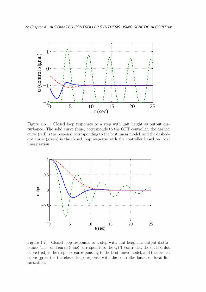
In this example the nonlinear system is a third order system, Hence we cannot usephase plane analysis to decide the selection of non-stationary points. One possibleway is to use simulation. Basically, we start with designing a controller only forthe desired operating point. Then we define the desired operating window andperturb the system with different step signals as the output disturbances. For thetrajectories that stay in the operating window, we can collect the data and addpoints from trajectories to the set of non-stationary points. As can be seen inFig. 4.7 and 4.8 adding non-stationary linearization points improves the robustnessand performance considerably. The derived PID controller also compares well to thecontroller based on the best linear model [15].

In [12] different optimization criteria for tuning the PID controllers are presented.To improve the performance in the foregoing example we can minimize ouput dis-turbance rejection criterion instead of the high frequency gain of the controller. i.e,

JLF = ‖S(s)‖∞ (4.20)

(4.21)

where S(s) is the sensitivity function.

The foregoing criterion is a measure of the system’s ability to handle LF outputdisturbances. The controller derived for this criterion is:

u = (0.588s2 + 0.614s + 0.336

s)e (4.22)


0 5 10 15 20 25−2

−1

0

1

t (sec)

u (c

ontr

ol s

igna

l)

Figure 4.6. Closed loop responses to a step with unit height as output dis-turbance. The solid curve (blue) corresponds to the QFT controller, the dashedcurve (red) is the response corresponding to the best linear model, and the dashed-dot curve (green) is the closed loop response with the controller based on locallinearization.

0 5 10 15 20 25−1

−0.5

0

0.5

1

t(sec)

outp

ut

Figure 4.7. Closed loop responses to a step with unit height as output distur-bance. The solid curve (blue) corresponds to the QFT controller, the dashed-dotcurve (red) is the response corresponding to the best linear model, and the dashedcurve (green) is the closed loop response with the controller based on local lin-earization.


0 5 10 15 20 25−2.5

−2

−1.5

−1

−0.5

0

0.5

1

1.5

2

t(sec)

outp

ut

Figure 4.8. Closed loop responses to the step with height two as the outputdisturbance. The solid curve (blue) corresponds to the QFT controller, the dashedcurve (red) is the response corresponding to the best linear model and the dashed-dot curve (green) is the closed loop response with the controller based on locallinearization.

Criterion H∞normJHF = KD 1.17

JLF = ‖S(s)‖∞ 1.11Best linear Model 1.14

Table 4.1. H∞ norm for different optimization criterion.

Fig. 4.9 and 4.10 illustrate the output and control activity for different controllersto the output disturbance. As can be seen, with this new criterion, we could furtherimprove the performance of the system.

One might ask if it is fair to compare a PI controller with a PID controller design.To answer this question, we should note that the idea here is not to compare ourPID design with the PI design in [15]. With this comparison we would like to showthat, the outcome from the presented method is as satisfactory as the result fromthe method given in [15].

To show the importance of the optimization criterion in our design, the Wienersystem is simulated for a process disturbance instead of the output disturbance thistime. Another controller is also designed to reject the LF process disturbance. Thefollowing criterion is used in the optimization algorithm:

JLF = ‖S(s)P (s)‖∞ (4.23)


0 5 10 15 20 25−2.5

−2

−1.5

−1

−0.5

0

0.5

1

1.5

2

t (Sec)

y (o

utpu

t)

HFLFB.ML.M

Figure 4.9. The dashed curve (red) is the closed loop response to the stepwith height two as the output disturbance for the best linear model, the dashed-dot curve (blue) is the response for the QFT designed controller with the highfrequency gain of the controller as the cost function to be minimized, the solidcurve (green) is the output for the QFT controller with LF output disturbancerejection as the objective function and eventually the dotted curve(purple) is thecontroller for the local linear model.

where S(s) is the sensitivity function and P (s) is the plant transfer function. Thederived controller is then

u = (0.684s2 + 0.584s + 0.526

s)e (4.24)

Fig. 4.11 and 4.12 show that the designed controller for the LF output disturbancerejection might not have the same behavior for other purposes. In other word, weobserve that although the designed controller for the best linear model shows a goodbehavior in rejecting the output disturbance but its response is deteriorated whena process disturbance is applied to the system. The presented method in this worknot only improve robustness but can be easily optimized with our algorithm withrespect to different desired criterion. Hence, robustness, simplicity and flexibilityare of the characteristics of the proposed algorithm.


0 5 10 15 20 25−1.8

−1.6

−1.4

−1.2

−1

−0.8

−0.6

−0.4

t (Sec)

Con

trol

sig

nal (

u)

Figure 4.10. The dashed curve (red) is the control signal for the controllerdesigned for the best linear model, The solid curve (green) is the control signalfor the PID controller design to minimize the effect of LF output disturbance andthe dashed-dot curve (blue) is the control signal for the PID controller with thehigh frequency gain of the controller as the cost function

0 5 10 15 20 25−0.2

0

0.2

0.4

0.6

0.8

1

1.2

t (Sec)

outp

ut (

y)

Best ModelHFLF

Figure 4.11. Closed loop responses to a step with height one as the processdisturbance. The solid curve (purple) corresponds to the QFT controller, thedashed curve (red) is the response corresponding to the best linear model, andthe dashed-dot curve (blue) is the closed loop response with the controller basedon local linearization.


0 5 10 15 20 25−1.4

−1.2

−1

−0.8

−0.6

−0.4

−0.2

0

t (Sec)

Con

trol

sig

nal (

u)

HFB.MLF

Figure 4.12. The solid curve (purple) is the control signal corresponds to theQFT controller which is designed with respect to process disturbance rejectioncriterion, the dashed curve (red) is the control signal corresponding to the bestlinear model, and the dashed-dot curve (blue) is the control signal for the con-troller which has the minimum high frequency gain.

5 BENCHMARK PROBLEM 1

5.1 MODELING

In order to further evaluate the performance and characteristics of our method, wehave selected a Bioreactor Benchmark problem as the plant to be controlled dueto its interesting characteristic [13]. Although this process is rather simple andhas only two state variables, it is difficult to control due to strong nonlinearity.The bioreactor is a continuous flow stirred tank reactor (CSTR) with water andcells (e.g., yeast or bacteria) which consumes nutrients (’substrate’) and produceproducts (both desired and undesired) and more cells. The stated control problemis tracking a desired amount of cell mass.

Figure 5.1. Bioreactor with ρ as input and x1 as output

The state space equations of the plant are:

X1 = −X1ρ + X1(1−X2)eX2/γ (5.1)

X2 = −X2ρ + X1(1−X2)eX2/γ 1 + ρ

1 + ρ−X2

(5.2)

where X1 is dimensionless cell mass and X2 is nutrient conversion, defined as (SF −S)/SF , where SF is the concentration of nutrient in the feed to the reactor and S isthe concentration (of nutrient) in the reactor. The constraints on the state variablesare:

Ω : 0 ≤ X1, X2 ≤ 1

27

28 Chapter 5 BENCHMARK PROBLEM 1

ρ is the control signal, which is the flow rate through the reactor (0 ≤ ρ ≤ 2). Tohave a better understanding of these equations we will explain each term below:

The first term (−X1ρ) in (5.1) is the amount of cells leaving the tank and the second

term X1(1−X2)eX2ρ represents cell growth in the tank. The rate is proportional to

the current amount of cell and depends nonlinearly on the amount of X2. In (5.2),the first term (−X2) is the amount of nutrient leaving the tank and the second term

X1(1−X2)eX2/γ 1 + β

1 + β −X2

is the rate by which the nutrient is metabolized. The constants β and γ determinethe rate of cell growth and nutrient consumption. From the equations we may alsodeduce that cell growth in moderate nutrient concentrations is faster than at veryhigh or low conversion.

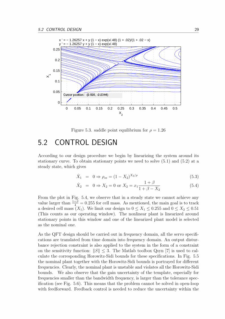
This system is a challenging benchmark because it is highly nonlinear and for somevalues of ρ limit cycle is unavoidable, see Fig. 5.2. The system is also unstable, ascan be seen in the phase portrait in Fig. 5.3. It can be noted that the system has onestable and one unstable eigenvalue in this area so the equilibrium points are saddlepoints. The system response is very sensitive to parameter variation. It means thata small error in the model can cause a large change in the control problem.

x ’ = − 1 x + y (1 − x) exp(x/.48) (1 + .02)/(1 + .02 − x)y ’ = − 1 y + y (1 − x) exp(x/.48)

0 0.1 0.2 0.3 0.4 0.5 0.6 0.7 0.8 0.9 1

0

0.05

0.1

0.15

0.2

0.25

0.3

0.35

0.4

X2

X1

Figure 5.2. Limit cycle for ρ = 1

5.2 CONTROL DESIGN 29

x ’ = − 1.26257 x + y (1 − x) exp(x/.48) (1 + .02)/(1 + .02 − x)y ’ = − 1.26257 y + y (1 − x) exp(x/.48)

0 0.05 0.1 0.15 0.2 0.25 0.3 0.35 0.4 0.45 0.5

0

0.05

0.1

0.15

0.2

0.25

X2

X1

Figure 5.3. saddle point equilibrium for ρ = 1.26

5.2 CONTROL DESIGN

According to our design procedure we begin by linearizing the system around itsstationary curve. To obtain stationary points we need to solve (5.1) and (5.2) at asteady state, which gives

X1 = 0 ⇒ ρss = (1−X2)X2/ρ (5.3)

X2 = 0 ⇒ X2 = 0 or X2 = x11 + β

1 + β −X2

(5.4)

From the plot in Fig. 5.4, we observe that in a steady state we cannot achieve anyvalue larger than 1+β

4= 0.255 for cell mass. As mentioned, the main goal is to track

a desired cell mass (X1). We limit our design to 0 ≤ X1 ≤ 0.255 and 0 ≤ X2 ≤ 0.51(This counts as our operating window). The nonlinear plant is linearized aroundstationary points in this window and one of the linearized plant model is selectedas the nominal one.

As the QFT design should be carried out in frequency domain, all the servo specifi-cations are translated from time domain into frequency domain. An output distur-bance rejection constraint is also applied to the system in the form of a constrainton the sensitivity function: ‖S‖ ≤ 3. The Matlab toolbox Qsyn [7] is used to cal-culate the corresponding Horowitz-Sidi bounds for these specifications. In Fig. 5.5the nominal plant together with the Horowitz-Sidi bounds is portrayed for differentfrequencies. Clearly, the nominal plant is unstable and violates all the Horowitz-Sidibounds. We also observe that the gain uncertainty of the template, especially forfrequencies smaller than the bandwidth frequency, is larger than the tolerance spec-ification (see Fig. 5.6). This means that the problem cannot be solved in open-loopwith feedforward. Feedback control is needed to reduce the uncertainty within the


0 0.2 0.4 0.6 0.8 10

0.05

0.1

0.15

0.2

0.25

0.3

0.35

X2

X1

Figure 5.4. Stationary points for the benchmark bioreactor

−350 −300 −250 −200 −150 −100 −50 0

−40

−30

−20

−10

0

10

20

30

40

50

1263

1

0.5

0.25

0

−50

−40

−30

−20

−12

−6

−3

−1−1

−3

−6

−12

−20

−30

−40

0

0.25

0.5

1

3612

Mag

[dB

]

Nichols Chart

0.05

0.10.2

0.5

1141050

0.050.1

0.2

0.5

1

4 10500.050.10.20.5

1

4

10

50

Figure 5.5. The blue curve to the left is nominal loop transfer function beforedesign and the pepper thick curve to the right is the loop transfer function afterdesign for only stationary points

5.2 CONTROL DESIGN 31

10−1

100

101

102

−20

0

20

rad/s

dB

Figure 5.6. The blue curve is nominal plant. Small circles, show the uncertaintiesdefined by the template. The red envelope is servo specification.

acceptable envelope. The idea here is to automatically design a PID controller insuch a way that the closed loop system becomes stable and fulfill the specificationsfor all frequencies. Preferably it should also be robust to initial error or deviationsfrom a steady state. The controller has the the following (ideal) transfer function:

G(s) =KDs2 + KP s + KI

s(5.5)

The optimization variables are θ = [KD, KP , KI ]>, and the objective function we

minimize is KD (high frequency gain of controller) subject to the following specifi-cations:

• Servo specification

a(ω) ≤∣∣∣∣F (jω)G(jω)P (jω)

1 + G(jω)P (jω)

∣∣∣∣ ≤ b(ω) (5.6)

• Sensitivity specification∣∣∣∣

1

1 + G(jω)P (jω)

∣∣∣∣ ≤ 3 (5.7)

Fig. 5.5 shows the nominal loop transfer function after design of the PID controller.From the plot we can see that the system becomes stable and the nominal looptransfer function satisfies the specifications for all frequencies. However, we cannotclaim that it has the desired performance on the original nonlinear system unless wetest our design through simulation. When we simulate the system from an initialcondition in a region close enough to the stationary points, the system response issatisfactory but for larger perturbations from equilibrium points in initial condition


−350 −300 −250 −200 −150 −100 −50 0

−40

−30

−20

−10

0

10

20

30

40

50

1263

1

0.5

0.25

0

−60

−50

−40

−30

−20

−12

−6

−3

−1−1

−3

−6

−12

−20

−30

−40

−50

−60

0

0.25

0.5

1

3612

Mag

[dB]

Phase [degree]

Nichols Chart

0.050.1

0.20.5

1

1014

1050

0.050.1

0.20.5

1

4

10

50

Figure 5.7. The blue curve is nominal loop transfer function after designing thecontroller

the system becomes unstable. These new non-stationary points are then added tothe set of linearization points iteratively. This imposes tougher boundaries on thenominal loop transfer function L0(jωk) in the Nichols chart (see Fig. 5.7). Weshould note that by selecting these new non-stationary points we aimed to makeour design more robust. The results shows the improvement in robustness butone should have in mind that there is limitation for selecting these non-stationarypoints. One possible limitation is that if we pick these non-stationary points too farfrom the equilibrium curve (or operating points) the uncertainty in the plant willincrease such that might make it impossible for the optimization algorithm to finda feasible solution. One good way to overcome this problem might be to start witha reasonable size of operating window in the state-space and try to design for thatand then iteratively enlarge the window. The problem is then solved with geneticalgorithm once more. We did not consider any initial guess for the optimizationalgorithm and the population size is set to 50. After five iteration the algorithmfound the solution. This process took almost 20 min. The simulation results forthis new controller, the former one and a sliding mode solution [4]is presented inthe next section. In Fig. 5.8 the gain extent of the closed loop system togetherwith the uncertainty in the template is portrayed. We see that after designing thefeedback the uncertainty is reduced to an acceptable level. We also conclude thatthere appears to be no need to design a prefilter F (s).

5.3 Simulation results 33

10−1

100

101

−20

0

20

rad/s

dB

Figure 5.8. The blue curve is nominal plant, the small circles show the uncer-tainty in the template, and the red envelope is the servo specification.

5.3 Simulation results

Simulations were carried out in Simulink for different initial values and differentsquare waves as reference signal. First of all the two controllers, one derived from lin-earization around only stationary points and another one from linearization aroundboth stationary and non-stationary points, are simulated for two different initialvalues. For an initial condition close enough to the stationary curve both con-trollers work, but as can be seen in Fig. 5.9 for an initial condition x1(0) = 0.15and x2(0) = 0.3 the controller designed for stationary points only results in largeovershoots. In Fig.14 we perturbed the system harder by giving an initial conditionx1(0) = 0.09 and x2(0) = 0.4 . For this rather large deviation from the stationarycurve the first controller gives an unstable response but the second one is more ro-bust and shows a satisfactory response. In [4] a sliding mode controller is designedfor this system. In Fig. 5.11 and 5.12 that sliding mode controller is compared tothe PID controller designed with the QFT method. The minimum and maximumvalues of the square wave are close to the maximum values that the system canreach. The systems are simulated for two different initial values that cause largeinitial errors in the control. As can be seen in Fig. 5.11 and 5.12 the PID controllerresponse has an acceptable response though a significant overshoot. However, froman implementation point of view the PID controller is clearly preferable.


0 100 200 300 4000.05

0.1

0.15

0.2

0.25

0.3

T(sec)

X1

Figure 5.9. Red dashed line is reference signal, blue curve is for controllerdesigned using non-stationary points and the green response is the response fromcontroller designed for stationary points only.

0 100 200 300 4000.05

0.1

0.15

0.2

0.25

0.3

T(sec)

X1

Figure 5.10. Red dashed is reference signal, blue curve is for the controller de-signed with QFT for non-stationary points and the green response is the responsefor the controller designed for stationary points only.

5.3 Simulation results 35

0 100 200 300 4000

0.05

0.1

0.15

0.2

0.25

T(sec)

X1

Figure 5.11. Red dashed line is the reference signal, blue is for the PID con-troller and the green one is for the sliding mode controller response. x1(0) =0.15, x2(0) = 0.2

0 100 200 300 4000

0.05

0.1

0.15

0.2

0.25

T(sec)

X!

Figure 5.12. Red dash line is the reference signal, the blue one is the QFTcontroller and the green one is the sliding mode controller response. x1(0) =0.05, x2(0) = 0.3

6 BENCHMARK PROBLEM 2

6.1 MODELING

The example which is considered in this chapter is a fourth order continuous stirredtank reactor (CSTR). In this process the desired product is cyclopentenol (substanceB) which is produced from cyclopentadiene (Substance A). In addition to the desiredproduct two other undesired products, dicyclopentadience (D) and cyclopentanediol(C), are produced as shown below.

AK1−→ B

K2−→ C (6.1)

2AK3−→ D (6.2)

The state space equations of the systems are

q,A,B,C,D

Q

q,A

.

Figure 6.1. Bioreactor with q as input and cB as output

cA =q

VR

(cA0 − cA)−K1cA −K3c2A (6.3)

cB = − q

VR

cB + K1cA −K2cB (6.4)

T =q

VR

(T0 − T ) +KW AR

ρCpVR

(Tc − T )− 1

ρCp

(K1cA∆HR,AB

+ K2cB∆HR,BC + K3c2A∆HR,AD) (6.5)

Tc =1

mcCpc

(Q + KW AR(T − Tc)) (6.6)

36

6.2 Controller design 37

Model Parameters Main operating pointK01,2 = (1.287± 0.04) · 1012h−1 cA|s = 1.235mol/l

K03 = (9.043± 0.27) · 1091/(molAh) cB|s = 0.9mol/lEA1,2/R = 9758.3K ±∆ T|s = 134.14CEA3/R = 8560.0K ±∆ Tc|s = 128.95C

∆HABR = 4.2± 2.36kJ/molA q = 188.3h−1

∆HBCR = −11.0± 1.92kJ/molB Q|s = −4495.7kJ/h

∆HADR = −41.85± 1.41kJ/molA ca0|s mol/l

ρ = 0.9342kg/l Cp = 3.01kJ/kgKCpk = 2kJ/kgK AR = 0.215m2

VR = 10.01 mk = 5.0kgT0 = 130C KW = 4032

Table 6.1. H∞ norm for different optimization criterion.

where K1,K2 and K3 are the reaction rate coefficient given by

Ki = Ki0eEi/(T/C+273.15), i = 1, 2, 3

cA and cB are the concentrations of the substances A and B respectively. T isthe temperature of the bioreactor and Tc is the temperature in the cooling jacket.Q is the heat flow which is removed from the coolant and finally q is the feedflow to the reactor containing substance A with the concentration cA0. The valuesfor the constant parameters and the main steady state operating point are givenin Table 6.1. Generally, this control problem is treated as a MIMO system withconcentration of substance B and temperature in the reactor (T ) as the outputs,and inflow q and heat flow Q as the control input [3]. However, we consider Qconstant (steady state value) and try to track the desired set point concentrationcB using q only. Hence, the problem is translated to a single input single outputproblem with q as the input an cB as the output. The desired operating window isconsidered in a suboptimal region relatively close to the maximum yield , i.e;

0.8 ≤ cB ≤ 1

The stationary curve for the two states ( cA and cB) is illustrated in Fig. 6.2. (Q,Tand Tc are kept at their steady state values). Although this process shows inputmultiplicity for some values of cA and cB but there is no need to be concern aboutthat in our desired operating window.

6.2 Controller design

In [15] the nonlinear system is approximated by a best linear model. With sim-ulation of the open loop system, they have shown that their best linear model issuperior to the locally linearized model in approximating the behaviour of the non-linear system. Finally, in their work they have designed an H∞ controller (C(s))


1 1.5 2 2.5 3 3.50.75

0.8

0.85

0.9

0.95

1

1.05

1.1

1.15

cA

c B

Figure 6.2. Stationary points

which is followed by a PI controller to track the desired set points for concentrationof substance B. The control signal is limited to 88.3 ≤ q ≤ 288.3 and the controlleris as below:

C(s) =1.040 · 103s3 + 1.020 · 106s2 + 4.274 · 107s + 3.563 · 108

s4 + 1.024 · 103s3 + 8.289 · 104s2 + 9.958 · 105s + 2.683 · 106(6.7)

u = (1 +25

s)C(s)e (6.8)

where e is the control error and u is the controller output.

In our work we tried to find a lower order controller which shows similar behavioras their H∞ controller designed for the Best linear model. A similar method that isshown in the two previous chapter is used to design a simple linear controller. Thedesign procedure can be summarized by the following steps:

• First the nonlinear system is linearized around its stationary points for cB ∈[0.8, 1].

• To add non-stationary points to the uncertainty set, the open loop system issimulated for small steps within q ∈ [88, 288] (see Fig. 6.3). The trajecto-ries of the responses are saved and used as the non-stationary points in thelinearization.

• The servo and sensitivity specifications are translated into the frequency do-main and HS-bounds are generated for the Nichols diagram. The sensitivity


0 0.2 0.4 0.6 0.8 1

0.65

0.7

0.75

0.8

0.85

0.9

0.95

1

1.05

1.1

Time (h)

Pla

nt o

utpu

t (m

ol/l)

Figure 6.3. Step responses of open loop system for different step sizes.

function should be ‖S(s)‖ ≤ 2.5 and for the servo specification a settling timeTs = 2h and maximum overshoot |MT | ≤ 10 percent are specified. As can beseen in Fig. 6.4 and 6.5 The results of adding these non-stationary points tothe set produces a bit tougher Horowitz-Sidi bounds in the Nichols diagram(c.f.Fig. 6.4 and 6.5.

−350 −300 −250 −200 −150 −100 −50−50

−40

−30

−20

−10

0

10

20

30

40

126

3

1

0.5

0.25

0

−50

−40

−30

−20

−12

−6

−3

−1−1

−3

−6

−12

−20

−30

−40

−50

0

0.25

0.5

1

3

612

Mag

[dB

]

Phase [degree]

Nichols Chart

0.150.2

0.3

0.5

11.5

220

1.5 24 10

0.2

0.3

0.5

Figure 6.4. Horowiz-Sidi Bounds for templates derived from only stationarypoints

• Genetic algorithm is used to do loop-shaping automatically for a fixed structure


−350 −300 −250 −200 −150 −100 −50 0−50

−40

−30

−20

−10

0

10

20

30

40

126

3

1

0.5

0.25

0

−50

−40

−30

−20

−12

−6

−3

−1−1

−3

−6

−12

−20

−30

−40

−50

0

0.25

0.5

1

3

612

Mag

[dB

]

Phase [degree]

Nichols Chart

0.150.2

0.3

0.5

11.5

220

1.52410

Figure 6.5. Horowiz-Sidi Bounds for templates derived from stationary andnon-stationary points

fourth order controller.

G(s) =θ(1)s2 + θ(2)s + θ(3)

s(s3 + θ(4)s2 + θ(5)s + θ(6)), (6.9)

where x is the optimization variable which is determined by the optimizationalgorithm. The objective function of optimization algorithm is J = θ(1) whichis the high frequency gain of the controller.

The designed controller has the transfer function as below:

G(s) =3358.454s2 + 63076.673s + 87689.366

s(s3 + 14.323s2 + 21.262s + 28.202)(6.10)

The simulation results for the controller designed using QFT and the controllerdesigned based on H∞ are illustrated in Fig. 6.6 and 6.7. It can be seen that thecontrollers have a very similar response. From the implementation point of view,using a fourth order controller is an advantageous over using a fifth order controller.Here we used the high frequency gain of the controller as the objective functionto be minimized as for the Wiener problem. Furthermore, it is possible to usedifferent criteria for different objectives. This possibility increases the flexibility ofthe method and in contrast to the Best linear model method we do not need to docomplex calculations to find the best linear model. In summary, we can mentionthe features of this method in general and compared to other methods.

• Control of nonlinear plant using linear controller.


• Using our automated controller synthesis makes the design procedure verysimple.

• Selection of non-stationary points carried out through simulation automati-cally.

• The designer has control over the structure and order of the controller. Inresult of this advantage, we succeed to design a controller with lower orderthan the H∞ controller in [15].

• By linearizing around a set of stationary and non-stationary points, we im-proved the approximation of the nonlinear system. Hence, there is no need tocalculate the best linear model with complicated calculation.

• Contrary to the proposed method in [15], our method is neither limited tostable plants nor to plants with time-delay.

0 0.5 1 1.5 2 2.5 3 3.5 40.75

0.8

0.85

0.9

0.95

1

1.05

Time (h)

Out

put

Figure 6.6. The dashed curves (green) are the closed loop step responses of theH∞ controller which is followed with a PI controller and the solid curves (blue)are the closed loop responses for the controller designed using QFT.

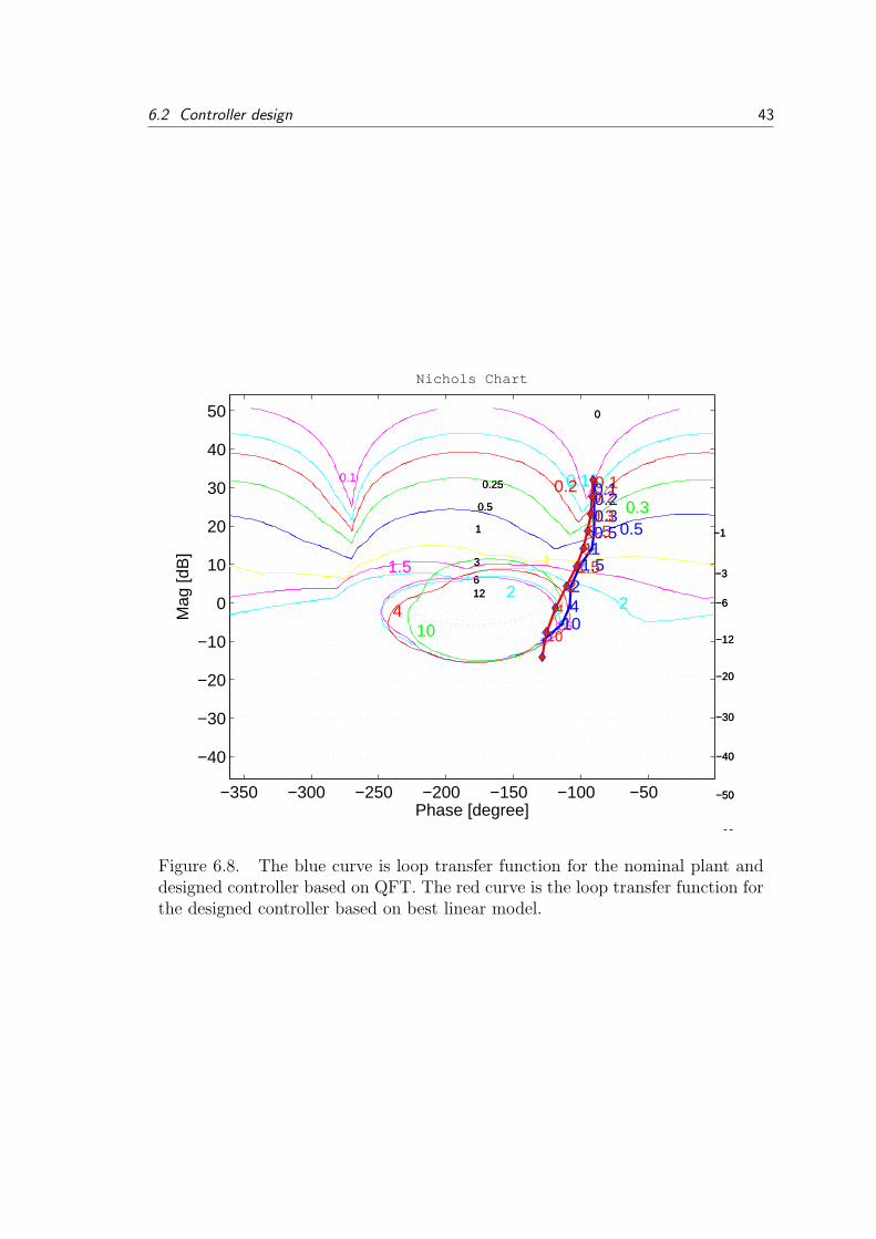
The loop transfer function for both cases of H∞ and QFT controllers are shown inthe Nichols diagram. It is interesting to see that the H∞ controller has a suprisinglysimilar loop transfer function to the QFT controller. We note that the phase of theQFT controller is slightly better than the phase for the H∞ controller.


0 0.5 1 1.5 2 2.5 3 3.5 4

100

150

200

250

300

Time (h)

Con

trol

sig

nal

Figure 6.7. The dashed curves (green) are the control activity signals of the H∞controller which is followed with a PI controller and the solid curves (blue) arethe control signals for the controller designed based on QFT.


−350 −300 −250 −200 −150 −100 −50

−40

−30

−20

−10

0

10

20

30

40

50

126

3

1

0.5

0.25

0

−60

−50

−40

−30

−20

−12

−6

−3

−1−1

−3

−6

−12

−20

−30

−40

−50

−60

0

0.25

0.5

1

3

612

Mag

[dB

]

Phase [degree]

Nichols Chart

0.1 0.150.20.3

0.5

11.5

21.5

24

10

0.10.20.30.51

1.524

10

0.10.20.30.51

1.52

4

10

Figure 6.8. The blue curve is loop transfer function for the nominal plant anddesigned controller based on QFT. The red curve is the loop transfer function forthe designed controller based on best linear model.

7 Conclusion

7.1 Conclusion

In this work a method based on linear QFT is used to design simple linear con-trollers for mildly nonlinear systems. The design is based on local linearization ofthe nonlinear system. In addition to the classical linearization around only equilib-rium points, non-equilibrium points are taken into account as well. One nominalloop transfer function is considered as the nominal plant and the rest are treatedas an uncertainty description for the nominal one. In order to facilitate the manualloop shaping in the Nichols diagram, the loop-shaping problem is translated to anoptimization problem with Horowitz-Sidi bounds as the optimization constraints.It has been shown by choosing an appropriate cost function for different controltarget, the result is improved. To solve the optimization problem with non-convexand nonlinear constraints, genetic algorithm is used. The efficiency of this algo-rithm has been shown in some examples. The linearization around non-stationarypoints improved both transient response and robustness of our design. This fact isshown through an example which is a second order unstable bioreactor benchmarkproblem. The method is also successfully applied to a fourth order CSTR bench-mark problem. In this problem the selection of non-stationary points is carried outthrough simulations of the open loop system for small step sizes as references.

7.2 Future Work

In this work genetic algorithm is used to find the coefficients of a fixed structurecontroller transfer function. It is possible to include the controller order selection inthe optimization algorithm. One important aspect in the presented method is theselection of non-stationary points. In this work, this selection is carried out throughphase plane analysis for second order systems, simulation of open loop system forstable plants, and simulation of closed loop system for unstable plant. (A controllerwhich stabilizes the main operating window is used in the simulation). If this taskis carried out on basis of solid theory it may result in a very powerful and usefulmethod to feedback design of nonlinear systems.

44

Bibliography

[1] A. Bafios, O. Yaniv, and F.J. Montoya. Nonlinear QFT based on local lin-earization. International Journal of Control, 2003.

[2] A. Banos. Nonlinear quantitative feedback theory. International Journal ofRobust And Nonlinear Control, 17:181-202, 2007.

[3] H. Chen, A. Kremling, and F. Allgower. Nonlinear predictive control of abenchmark cstr. Proceeding of 3rd Eurpean Control Conference, Rome, Italy,Sep 1995.

[4] Mehmet Onder Efe. Model refernce sliding mode control for bioreactor bench-mark problem. International Workshop on Variable Structure Systems, 2008.

[5] C. Fransson, T. Wik, B. Lennartson, M. Saunders, and P. Gutman. Non-conservative robust control: Optimized and constrained sensitivity functions.IEEE Transactions on Control Systems Technology, 17:298-308, May 2009.

[6] C. M. Fransson, B. Lennartson, T. Wik, and K. Holmstrom. Multi criteria con-troller design for uncertain MIMO systems using nonconvex global optimiza-tion. In 40th IEEE Conference on Decision and Control, volume 1-5, pages3976–3981, Orlando, FL, USA, Dec 2001.

[7] P.O. Gutman. Manual for the toolbox for Robust Control System Design foruse with Matlab, May 1996.

[8] Issac Horowitz. Survey of quantitative feedback theory (qft). InternationalJournal of Robust and Nonlinear Control, 2001.

[9] I. Horwitz. Quantitative Feedback Design Theory. QFT Publications., 1993.

[10] T. A. Johansen, K. J. Hunt, P. J. Gawthrop, and H. Fritz. Off-equilibriumlinearisation and design of gain-scheduled control with application to vehiclespeed control. pages: 167-180. Control enginnering practice, 1998.

[11] H. Khalil. Nonlinear systems. Prentice Hall., 2003.

[12] B. Kristiansson and B. Lennartson. Robust tuning of PI and PID controllers.IEEE Control Systems Magazine, Feb 2006.

[13] W. T. Miller, R. S. Sutton, and P. J. Werbos. Neural Networks for Control.MIT Press, pp.387-402, 1990.

[14] T. Schweickhardt and F. Allgower. Linear control of nonlinear systems basedon nonlinearity measures. J. Process Control, 17:273–284, 2007.

45

46 BIBLIOGRAPHY

[15] T. Schweickhardt and F. Allgower. A robustness approach to linear control ofmildly nonlinear processes. International Journal of Robust Control, 17:1163–1182, 2007.

[16] T. Schweickhardt and F. Allgower. On system gains, nonlinearity measures, andlinear models for nonlinear systems. IEEE transactions on automatic control,54(1):62–78, 2009.

[17] T. Wik, C. M. Fransson, and B. Lennartson. Feedforward feedback controllerdesign for uncertain systems. In 42th IEEE Conference on Decision and Con-trol, pages 5328–5334, Maui, Hawaii, USA, Dec 2003.

Documents

Automated Linear Controller Design For Mildly …publications.lib.chalmers.se/records/fulltext/99384.pdf · Automated Linear Controller Design For Mildly Nonlinear Systems Using Quantitative