Automated Remote Sensing with Near Infrared Reflectance Spectra: Carbonate Recognition

Joseph Ramsey, Paul Gazis, Ted Roush, Peter Spirtes and Clark Glymour1

Abstract

Reflectance spectroscopy is a standard tool for studying the mineral composition of rock and soil samples and for remote sensing of terrestrial and extraterrestrial surfaces. We describe research on automated methods of mineral identification from reflectance spectra and give evidence that a simple algorithm, adapted from a well-known search procedure for Bayes nets, identifies the most frequently occurring classes of carbonates with reliability equal to or greater than that of human experts. We compare the reliability of the procedure to the reliability of several other automated methods adapted to the same purpose. Evidence is given that the procedure can be applied to some other mineral classes as well. Since the procedure is fast with low memory requirements, it is suitable for on-board scientific analysis by orbiters or surface rovers.

1. Introduction.

The identification of surface composition from reflectance spectra has

traditionally relied on two methods. The older of the two is a direct examination of

spectra by experts, seeking lines or bands characteristic of particular substances,

sometimes taking account of overall luminosity of the spectrum, and sometimes, with

computational aids, taking account of the shapes of bands. The standard alternative is

simultaneous linear regression of an unknown spectrum against a library of known

spectra for candidate materials; a number of spectral libraries have been compiled which

can be used for this purpose. Some neural net procedures have also been used to analyze

2

spectral data, typically not for identifying surface composition directly, but rather for

finding bounded regions of similar composition in an array of point spectra from a

“visual” field. Other automated techniques have been explicitly used to identify surface

composition of minerals and rocks, including a Bayesian technique described below.

However, despite its numerous applications for planetary and terrestrial exploration and

for various military purposes, we have found no published systematic (or unsystematic)

study comparing automated classification of reflectance spectra to human expert

classification of reflectance spectra, nor any systematic comparative study of alternative

automated procedures. Using a both laboratory and field data sets, this paper provides

such comparisons.

So far as planetary exploration is concerned, reflectance spectroscopy techniques

have already shown themselves to be useful. Near-infrared reflectance spectroscopy

(from approximately 0.4 µm to 2.5 µm) in particular has offered geologists an important

potential source of petrological information for planetary, satellite and other solar system

exploration. Lightweight, low-power commercial instrumentation is available, detailed

physical models have been developed (e.g. Hapke 1993), and such data is routinely used

by geological spectroscopists in practical mineral classification (see, for example,

Chapters 3, 14, 16, 20, and 21 of Pieters and Englert, 1993 and references therein). Were

such instruments coupled with intelligent software for mineral classification from spectra,

the resulting system could be used for either remote sensing or surface based studies,

reducing data storage and information transmission requirements and aiding autonomous,

rational, scientifically-informed decisions by robot explorers about further directions for

exploration and data acquisition.

3

This interest in planetary exploration motivates an examination of the problem of

determining whether rock or soil samples contain carbonates and, in particular, whether

such samples contain either of the most frequently occurring forms of carbonate

material—calcite or dolomite. Carbonate identification is interesting for extra-terrestrial

exploration, because carbonates are typically formed by processes—such as deposition

from water—which could indicate a history of an environment that once supported life.

We therefore, focus on the task of carbonate identification. We compare the reliabilities

of (a) an expert human spectroscopist, (b) an expert system that models human expert

procedures, and (c) a variety of automated techniques, including linear regression, each

with various resampling and cross-validation techniques, on the task of carbonate

identification from visual to near infrared reflectance spectra. All of our tests of data

mining procedures use the same library of spectra for training or reference. A variety of

data sets are used for testing, including laboratory and field spectra obtained under

various conditions.

In our tests, an adaptation of the PC algorithm (Spirtes et al., 1993, 2001)

implemented in the TETRAD II program (Scheines et al., 1994) for constructing causal

Bayes nets from data, combined with appropriate data selection and data preprocessing,

performed more reliably than any other automated procedure we have tested. We will

refer to this procedure as the “modified PC “ or “modified Tetrad” algorithm. In some

tests this procedure was more informative than a human expert spectroscopist and almost

as reliable, and in other tests the procedure performed almost as well as human experts

with access both to physical samples and to measured spectra of the physical samples.

These claims are made more precise in the data summaries given below. We additionally

4

compare various preprocessing and data selection procedures, and, through an experiment

comparing expert human performance and machine performance, we investigate the

likelihood that our techniques can be successfully applied to other classes of minerals.

2. Preprocessing of Data.

Raw spectral data are preprocessed in our analysis in a variety of ways to produce

data that can usefully be analyzed by automated techniques.

First, raw spectral data are converted to intensities by comparing them to spectra

from standard white samples measured under the same conditions. To compensate for

the varying power function of sunlight, digitalized spectra, taken in the field, are

automatically divided by the spectrum of a white reference surface placed near the target,

and these ratios are recorded for a number of channels—826 channels in the instrument

used in this study.2 These ratios are the intensities of the spectral measurements for their

respective channels. Different instruments covering the same wavelength interval may

use distinct wavelength channels, and comparisons of field spectra taken with one

instrument to laboratory spectra taken with another instrument require that the channels

for one of the instruments be used to interpolate values for the channels used in the other

instrument. This interpolation ensures that data submitted to identification algorithms

utilize the same set of wavelengths throughout.

Second, anomalous lines are removed from the spectrum. For various reasons, at

some wavelengths the output of a spectroscope in the field may have out-of-range

intensity values. For example, water vapor in the atmosphere often creates anomalous

absorption lines around 1.9 µm. These lines within each spectrum can be removed by

5

computational preprocessing, or they can be removed by hand, or the spectra themselves

can be tested automatically for extreme variation and extremal spectra rejected altogether

for analysis. We use the latter two procedures—removing anomalous lines by hand and

rejecting spectra with extremal variation—for spectra taken in the field in the

experiments described in this paper.

Third, hull differences of the spectrum are calculated. After any elimination of

out-of-range channels, the intensities for each of the remaining channels in a spectrum

can then be subjected to interpretation either directly—the data are the "raw" spectral

intensities—or after transformation. The most common transformation fits a piece-wise

linear "hull" around the extremal points of hills and valleys of the spectrum and

computes, for each channel, the difference between the spectral intensity at that channel

and the numerical value of the hull at that channel on the intensity scale. The "hull

difference" values are then subjected to analysis. An alternative but less successful

procedure is to compute first differences among intensities in successive channels. We

have found that a suitably loose hull difference works best.

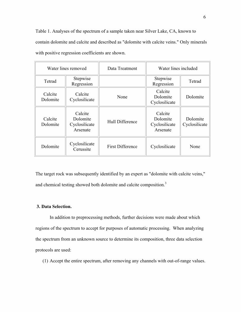
The effects of different preprocessing procedures are illustrated by analyses of the

spectrum of a rock taken near Silver Lake, CA; the results are shown in Table 1. The

composition of the rock was analyzed by two procedures, using the raw spectra, hull

differences, and first differences, with and without water lines removed. One of the

procedures was linear regression with a reference library of laboratory spectra from the

Jet Propulsion Laboratory (Grove et al. 1992) and the STEPWISE procedure in Minitab.

The other procedure was the modified PC algorithm, to be explained later in this paper.

6

Table 1. Analyses of the spectrum of a sample taken near Silver Lake, CA, known to

contain dolomite and calcite and described as "dolomite with calcite veins." Only minerals

with positive regression coefficients are shown.

Water lines removed Data Treatment Water lines included

Tetrad Stepwise Regression Stepwise

Regression Tetrad

Calcite Dolomite

Calcite Cyclosilicate None

Calcite Dolomite

Cyclosilicate Dolomite

Calcite Dolomite

Calcite Dolomite

Cyclosilicate Arsenate

Hull Difference

Calcite Dolomite

Cyclosilicate Arsenate

Dolomite Cyclosilicate

Dolomite Cyclosilicate Cerussite First Difference Cyclosilicate None

The target rock was subsequently identified by an expert as "dolomite with calcite veins,"

and chemical testing showed both dolomite and calcite composition.3

3. Data Selection.

In addition to preprocessing methods, further decisions were made about which

regions of the spectrum to accept for purposes of automatic processing. When analyzing

the spectrum from an unknown source to determine its composition, three data selection

protocols are used:

(1) Accept the entire spectrum, after removing any channels with out-of-range values.

7

(2) Accept only channels in a particular interval or union of intervals, when the

purpose is to recognize a particular component, or class of components, if present,

and this component, or class of components, is known to exhibit a distinctive

spectral features in this particular wavelength interval or set of intervals.

(3) Detect only particular spectral bands or lines characteristic of particular

components of interest, if present.

The advantage of the first strategy is evidently that it uses all of the data, but if only parts

of the spectrum provide a distinctive signal for a mineral class, use of the entire spectrum

may be a disadvantage. The advantage of the second strategy is that it makes efficient use

of background knowledge to focus on the informative part of the spectral signal; the

disadvantage is that the procedure reduces the size of the data set, which sometimes

makes statistical procedures inapplicable, as we will illustrate in subsequent sections. The

third strategy also makes use of background knowledge, but lines and bands

characteristic of the spectrum of a pure mineral may be shifted or masked in the spectrum

from a surface of mixed composition.

4. A Field Test of Automated Procedures and Data Selection Protocols.

In the winter of 1999, NASA scientists conducted field tests of a robot and

instruments in and about Silver Lake, California, a dry lake bed in the Mojave Desert

(Stoker et al. 2001). Among the instruments was a near-infrared spectrometer (Johnson et

al. 2001). Spectra were taken, usually in situ, of rocks and soils; the spectra were

identified as carbonates or non-carbonates both by the field geologists, from physical

observations of the specimens and their spectra, and by a group of geologists located

8

remotely at NASA Ames, who used both the spectra and the descriptions of the field

experts (Gazis and Roush 2001). Paul Gazis at NASA Ames provided software to correct

instrumental artifacts and to filter out spectra that, typically because of atmospheric

effects, were too noisy to process. After this pre-processing, 21 spectra remained; 13

samples were identified as carbonates and 8 samples identified as non-carbonates by the

field geologists. Subsequently, eight of the 21 samples were analyzed by standard

petrographic techniques. All eight analyses agreed with the judgements of the field

geologists and the remote geologists.

The data were analyzed using the following combinations of procedures. (The

details of the procedures, and their rationales, are explained in the next section.)

(1) The modified PC algorithm, seeking to recognize any carbonates, using a

restricted interval of wavelengths with intensity patterns characteristic of

carbonates.

(2) The modified PC algorithm, seeking to identify carbonates from calcites and

dolomites only, using a restricted interval of wavelengths with intensity patterns

characteristic of carbonates.

(3) The modified PC algorithm, seeking to recognize any carbonates, using all

wavelengths available from the instrument.

(4) The modified PC algorithm, seeking to recognize only calcites and dolomites,

using all wavelengths available from the instrument.

(5) Linear regression, seeking to recognize the presence of any carbonates using all

wavelengths available from the instrument.

9

(6) Linear regression, seeking to recognize the presence of any carbonates using all

wavelengths available from the instrument, but reporting only components with

positive regression coefficients.

(7) Linear regression, seeking to recognize carbonates from calcites or dolomites

only, using all wavelengths available from the instrument.

(8) Linear regression, seeking to recognize carbonates for calcites or dolomites only,

using all wavelengths available from the instrument, but reporting only

components with positive regression coefficients.

(9) An expert system seeking to recognize the presence of any carbonates from a

triple of lines around 2.3 µm. (Gazis and Roush 2001)

Because this data set has been incompletely described in at least two other published

reports, we give its composition in full in Tables 2 and 3. The field group’s name for

each sample is given in the leftmost columns of the tables.

10

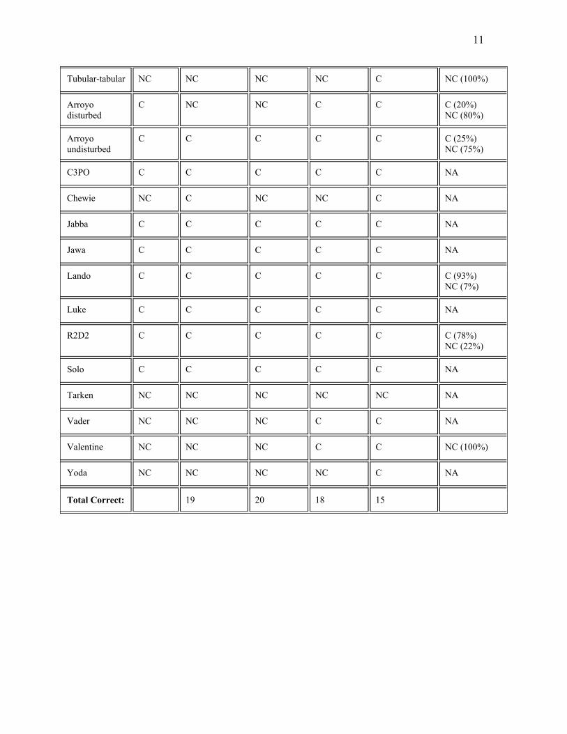
Table 2. Carbonate identifications of field spectra from Baker, CA using the modified PC

algorithm. The first column shows the nickname given to each sample for purposes of

analysis. The second column shows the carbonate ID of the rock by an expert in the

field. Columns 3 through 6 display carbonate identifications using the modified PC

algorithm, with different preparations of spectra and different criteria for carbonate

identification. In columns 3 and 4, all spectra are hull differenced and then truncated to

the interval [2.0, 2.5]; in columns 5 and 6, the spectra are hull differenced but not

truncated. In columns 3 and 6, a sample is counted as a carbonate if the modified PC

algorithm returns a set of minerals which contains any carbonate from among the 15

large-grain carbonates in the JPL mineral data set; in columns 4 and 5, a sample is

counted as a carbonate only if the modified PC algorithm returns a set containing a

calcite or a dolomite. Column 7 shows the results (where laboratory testing is available).

1. Sample

2. Field Expert ID

3. Modified PC ID (All carbonates; 2.0-2.5 µm)

4. Modified PC ID (Calcite or Dolomite Only; 2.0-2.5 µm)

5. Modified PC ID (Calcite or Dolomite Only; 0.4 – 2.5 µm)

6. Modified PC ID (All carbonates; 0.4 – 2.5 µm)

7. Laboratory ID

Emperor #1 C C C C C C (90%) NC (10%)

Emperor #2 C C C C C C (90%) NC (10%)

T 103 NC NC NC NC NC NA

T 105 NC NC NC C C NA

T 106 C C C C C NA

Endolith C C C C C C (93%) NC (7%)

11

Tubular-tabular NC NC NC NC C NC (100%)

Arroyo disturbed

C NC NC C C C (20%) NC (80%)

Arroyo undisturbed

C C C C C C (25%) NC (75%)

C3PO C C C C C NA

Chewie NC C NC NC C NA

Jabba C C C C C NA

Jawa C C C C C NA

Lando C C C C C C (93%) NC (7%)

Luke C C C C C NA

R2D2 C C C C C C (78%) NC (22%)

Solo C C C C C NA

Tarken NC NC NC NC NC NA

Vader NC NC NC C C NA

Valentine NC NC NC C C NC (100%)

Yoda NC NC NC NC C NA

Total Correct: 19 20 18 15

12

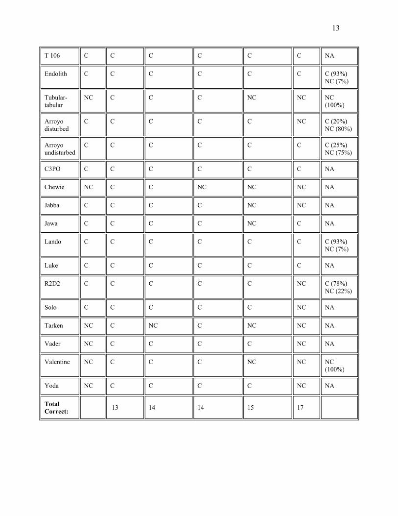
Table 3. Carbonate identifications of field spectra from Baker, CA using the

simultaneous linear regression algorithm in Minitab. Column 1 shows the nickname

given to each sample for purposes of analysis. Column 2 shows the carbonate ID of the

rock by an expert in the field. Columns 3 through 6 display carbonate identifications

using linear regression, with different criteria for carbonate identification. In columns 3

and 5, samples are counted as carbonates if when regressed onto the JPL library at least

one of the JPL carbonates has a significant regression coefficient; in columns 4 and 6,

this regression coefficient must be not only significant but also positive. Also, in

columns 3 and 4, a sample is counted as carbonate if when regressed any of the JPL

carbonates has a significant regression coefficient; in columns 5 an 6, only significant

regression coefficients for calcites and dolomites are counted. Column 7 shows the

identification by the expert system used in the study, and column 8 shows the results

(where available) of laboratory testing.

1. Sample

2. Field Expert ID

3. Regression ID (All carbonates; 0.4 – 2.5 µm)

4. Regression ID (All carbonates with positive coefficient; 0.4 – 2.5 µm)

5. Regression ID (Calcite or Dolomite Only; 0.4 – 2.5 µm)

6. Regression ID (Calcite or Dolomite Only, with positive coefficient; 0.4 – 2.5 µm)

7. Expert System ID

8. Laboratory ID

Emperor #1

C C C C C C C (90%) NC (10%)

Emperor #2

C C C C C C C (90%) NC (10%)

T 103 NC C C C C NC NA

T 105 NC C C C C NC NA

13

T 106 C C C C C C NA

Endolith C C C C C C C (93%) NC (7%)

Tubular-tabular

NC C C C NC NC NC (100%)

Arroyo disturbed

C C C C C NC C (20%) NC (80%)

Arroyo undisturbed

C C C C C C C (25%) NC (75%)

C3PO C C C C C C NA

Chewie NC C C NC NC NC NA

Jabba C C C C NC NC NA

Jawa C C C C NC C NA

Lando C C C C C C C (93%) NC (7%)

Luke C C C C C C NA

R2D2 C C C C C NC C (78%) NC (22%)

Solo C C C C C NC NA

Tarken NC C NC C NC NC NA

Vader NC C C C C NC NA

Valentine NC C C C NC NC NC (100%)

Yoda NC C C C C NC NA

Total Correct: 13 14 14 15 17

14

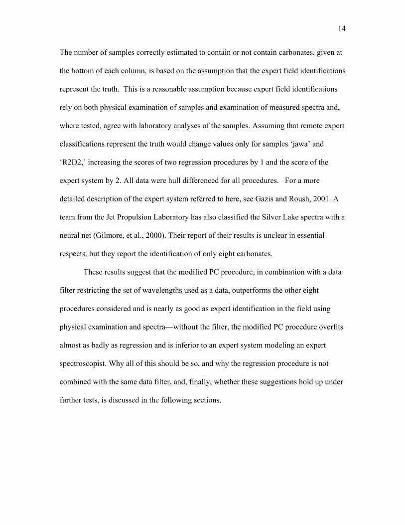
The number of samples correctly estimated to contain or not contain carbonates, given at

the bottom of each column, is based on the assumption that the expert field identifications

represent the truth. This is a reasonable assumption because expert field identifications

rely on both physical examination of samples and examination of measured spectra and,

where tested, agree with laboratory analyses of the samples. Assuming that remote expert

classifications represent the truth would change values only for samples ‘jawa’ and

‘R2D2,’ increasing the scores of two regression procedures by 1 and the score of the

expert system by 2. All data were hull differenced for all procedures. For a more

detailed description of the expert system referred to here, see Gazis and Roush, 2001. A

team from the Jet Propulsion Laboratory has also classified the Silver Lake spectra with a

neural net (Gilmore, et al., 2000). Their report of their results is unclear in essential

respects, but they report the identification of only eight carbonates.

These results suggest that the modified PC procedure, in combination with a data

filter restricting the set of wavelengths used as a data, outperforms the other eight

procedures considered and is nearly as good as expert identification in the field using

physical examination and spectra—without the filter, the modified PC procedure overfits

almost as badly as regression and is inferior to an expert system modeling an expert

spectroscopist. Why all of this should be so, and why the regression procedure is not

combined with the same data filter, and, finally, whether these suggestions hold up under

further tests, is discussed in the following sections.

15

5. Descriptions of the Automated Procedures.

5.1 Multiple Regression.

The regression procedure takes each channel wavelength as a unit and uses the

value of the intensity of the target rock at each measured wavelength as the dependent

variable. The independent variables are the intensities of each of the 135 large-grain

mineral samples in the JPL library of reflectance spectra, at the same wavelengths. The

135 minerals are divided into 17 classes, one of which is the carbonate class, with 15

minerals, including 3 dolomites and 2 calcites.4

In the regression procedure using all carbonates, a carbonate is recorded as

present if any of the 15 carbonates in the JPL library has a significant regression

coefficient, using a 0.05 significance level. In the regression procedure using only

calcites and dolomites, a carbonate is recorded as present if any of the five calcites or

dolomites has a significant regression coefficient, using a 0.05 significance level. In the

regression procedures requiring a positive sign, a carbonate is reported present if a

carbonate mineral has a significant positive coefficient. In only one case was the result

very sensitive to the significance level (an increase in the significance level to 0.054

would have resulted in the misclassification of ‘Chewie’ as a carbonate using either of the

two regression procedures that identify carbonates through calcites and dolomites.)

Otherwise, variations in the significance level between 0.100 and 0.010 would have made

no difference in the regression results.

Note that regression suffers from three difficulties, one structural and two

statistical, which make it an inferior procedure in many applications:

16

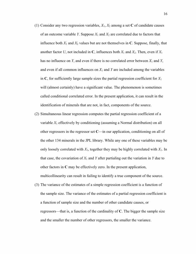
(1) Consider any two regression variables, X1, X2 among a set C of candidate causes

of an outcome variable Y. Suppose X1 and X2 are correlated due to factors that

influence both X1 and X2 values but are not themselves in C. Suppose, finally, that

another factor U, not included in C, influences both X1 and X2. Then, even if X1

has no influence on Y, and even if there is no correlated error between X1 and Y,

and even if all common influences on X1 and Y are included among the variables

in C, for sufficiently large sample sizes the partial regression coefficient for X1

will (almost certainly) have a significant value. The phenomenon is sometimes

called conditional correlated error. In the present application, it can result in the

identification of minerals that are not, in fact, components of the source.

(2) Simultaneous linear regression computes the partial regression coefficient of a

variable X1 effectively by conditioning (assuming a Normal distribution) on all

other regressors in the regressor set C—in our application, conditioning on all of

the other 134 minerals in the JPL library. While any one of these variables may be

only loosely correlated with X1, together they may be highly correlated with X1. In

that case, the covariation of X1 and Y after partialing out the variation in Y due to

other factors in C may be effectively zero. In the present application,

multicollinearity can result in failing to identify a true component of the source.

(3) The variance of the estimates of a simple regression coefficient is a function of

the sample size. The variance of the estimates of a partial regression coefficient is

a function of sample size and the number of other candidate causes, or

regressors—that is, a function of the cardinality of C. The bigger the sample size

and the smaller the number of other regressors, the smaller the variance.

17

Assuming a Normal distribution, the trade off is one for one: adding an extra

regressor variable is equivalent in its effect on the variance to reducing the sample

size by one unit. In the present application, reducing the number of channels used

for data analysis increases the variance of the estimates of regression coefficients.

In the extreme case in which the number of variables is greater than the sample

size, regression is ill-defined, and standard regression packages will not run at all.

In our application, regression procedures will not run using the JPL library as the

regressor set C and restricting the data to the channels with wavelengths in the

interval [2.0 µm, 2.5 µm].5

Several remedies to this last difficulty can be considered. The wavelength interval [2.0

µm, 2.5 µm], in this case, is chosen because previous work on carbonate spectra shows

that this region has distinctive spectral features for carbonates. We could search for a

larger range of wavelengths optimal for regression procedures in this application. We

could eliminate some of the minerals in the JPL library from the set of possible

components of the source, but that would decrease the reliability of the procedure when

those components or spectrally similar components are actually present in the source. We

could use a stepwise regression procedure, but other experiments with small samples

have found stepwise regression less reliable than the procedure used here (Spirtes et. al.,

1993, 2001). A better solution to this problem is available—viz., the algorithm described

in the next subsection.

18

5.2 The Modified PC Algorithm.

All three of the problems cited above with linear regression stem from a single

structural feature of the regression procedure, linear or otherwise. In estimating the

influence of a variable X on the outcome Y, regression conditions simultaneously on all

other candidate variables—i.e., all of the other members of C. That is, in our (rather

conventional, but not textbook) use of regression, we test the null hypothesis that X has

no influence on Y (or is not a component of Y) by using the distribution of a test statistic

that is conditioned on all other members of C.

There is an alternative procedure that minimizes the number of variables that must

be conditioned on. It takes as input a set of background variables C = {X1, X2, ...,

Xn}together with a target variable Y not in C and dynamically eliminates variables from

C using conditional independence facts, calculated from data. Variables are eliminated

which are independent of Y conditional on subsets of other remaining variables in C,

where the cardinality m of the subsets increases in size (m = 0, 1, 2, ...) until no more

variables can be eliminated from C. More formally:

Modified PC Algorithm:

Given set C of background variables and target variable Y:

(1) for each Xi in C, test the hypothesis that the correlation of Xi with Y is

zero; if the correlation of Xi with Y is zero, C:= C – {Xi};

(2) for each Xi in C, and for each Xj ≠ Xi in C, test the hypothesis that the

correlation Xi with Y, controlling for Xj , is zero; if the correlation of Xi

with It controlling for Xj is zero, C:= C – {Xi};

19

(3) for each Xi in C and each Xj, Xk ≠ Xi in C test the hypothesis that the

correlation Xi with Y, controlling for Xj , Xk is zero; if the correlation of Xi

with It controlling for Xj , Xk is zero C:= C – {Xi};

...and so on, until no more members of C can be removed. Return C.

This procedure may be understood intuitively as a application of the theory of search for

graphical causal models (Spirtes, et al, 1993, 2001), applied in this case to produce a

directed graph representing a hypothesis about the mineral composition of a source.

If n members of C are actually components of Y, no more than n variables must

be conditioned on simultaneously. If, for example, three minerals in the JPL library are

actual components of a sample, a large number of statistical tests will be done, but none

of the tests will require controlling for more than three variables—in no test will the

sample size effectively be reduced by more than 4, in contrast to multiple regression in

which the sample size is reduced by 134. For that reason, unlike multiple regression, the

procedure can be used with the JPL library with the reduced data set using only

intensities in channels for wavelengths in the interval [2.0 µm, 2.5 µm].

This procedure is subject to the statistical objection that no confidence intervals or

error probabilities can be calculated (see Robins, et al., 1999 and Spirtes, et al., 2000).

But, unlike regression, there is a proof that the procedure—under specified

assumptions—is asymptotically correct, and in simulation studies the procedure is much

more reliable than best subsets procedures (Spirtes, et al., 1993). While confidence

intervals have important uses, if the choice is between a procedure with confidence

intervals that is known to be asymptotically invalid and is unreliable in real applications

20

and in simulation studies and with small samples, or an asymptotically correct procedure

found to be reliable but admitting no confidence intervals, we prefer the latter.

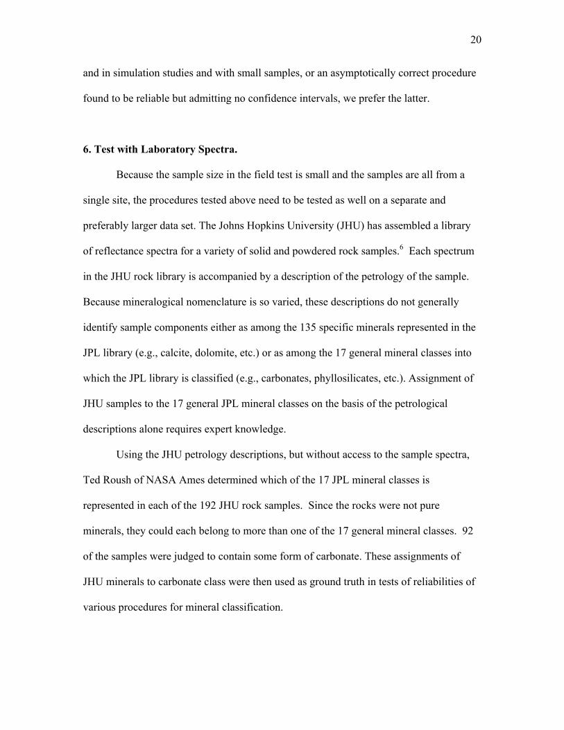
6. Test with Laboratory Spectra.

Because the sample size in the field test is small and the samples are all from a

single site, the procedures tested above need to be tested as well on a separate and

preferably larger data set. The Johns Hopkins University (JHU) has assembled a library

of reflectance spectra for a variety of solid and powdered rock samples.6 Each spectrum

in the JHU rock library is accompanied by a description of the petrology of the sample.

Because mineralogical nomenclature is so varied, these descriptions do not generally

identify sample components either as among the 135 specific minerals represented in the

JPL library (e.g., calcite, dolomite, etc.) or as among the 17 general mineral classes into

which the JPL library is classified (e.g., carbonates, phyllosilicates, etc.). Assignment of

JHU samples to the 17 general JPL mineral classes on the basis of the petrological

descriptions alone requires expert knowledge.

Using the JHU petrology descriptions, but without access to the sample spectra,

Ted Roush of NASA Ames determined which of the 17 JPL mineral classes is

represented in each of the 192 JHU rock samples. Since the rocks were not pure

minerals, they could each belong to more than one of the 17 general mineral classes. 92

of the samples were judged to contain some form of carbonate. These assignments of

JHU minerals to carbonate class were then used as ground truth in tests of reliabilities of

various procedures for mineral classification.

21

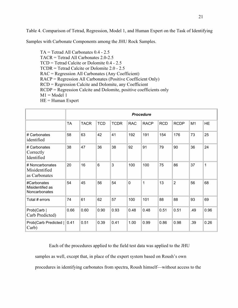
Table 4. Comparison of Tetrad, Regression, Model 1, and Human Expert on the Task of Identifying

Samples with Carbonate Components among the JHU Rock Samples.

TA = Tetrad All Carbonates 0.4 - 2.5 TACR = Tetrad All Carbonates 2.0-2.5 TCD = Tetrad Calcite or Dolomite 0.4 - 2.5 TCDR = Tetrad Calcite or Dolomite 2.0 - 2.5 RAC = Regression All Carbonates (Any Coefficient) RACP = Regression All Carbonates (Positive Coefficient Only) RCD = Regression Calcite and Dolomite, any Coefficient RCDP = Regression Calcite and Dolomite, positive coefficients only M1 = Model 1 HE = Human Expert

Procedure

TA TACR TCD TCDR RAC RACP RCD RCDP M1 HE

# Carbonates identified

58 63 42 41 192 191 154 176 73 25

# Carbonates Correctly Identified

38 47 36 38 92 91 79 90 36 24

# Noncarbonates Misidentified as Carbonates

20 16 6 3 100 100 75 86 37 1

#Carbonates Misidentifed as Noncarbonates

54 45 56 54 0 1 13 2 56 68

Total # errors 74 61 62 57 100 101 88 88 93 69

Prob(Carb | Carb Predicted)

0.66 0.60 0.90 0.93 0.48 0.48 0.51 0.51 .49 0.96

Prob(Carb Predicted | Carb)

0.41 0.51 0.39 0.41 1.00 0.99 0.86 0.98 .39 0.26

Each of the procedures applied to the field test data was applied to the JHU

samples as well, except that, in place of the expert system based on Roush’s own

procedures in identifying carbonates from spectra, Roush himself—without access to the

22

petrological descriptions of the samples—attempted to identify samples with carbonate

components. The results of these analyses are summarized in Table 4.

We recognized that among the machine classification algorithms available in the

artificial intelligence literature, there may be classifiers that perform better than the

modified PC algorithm. To search for such procedures, we used the Model 1 program, a

commercial program that uses a training set—in our study, the JPL library—to assess the

performance of a large number of algorithms. We tested one of the best-scoring

algorithms found by Model 1 on the JHU library. The procedures among which Model 1

searched included include linear regression, cross-validated linear regression, logistic

regression, cross validated logistic regression, backpropagation on a neural network,

cross-validated backpropagation, CART (classification and regression trees), naïve

Bayes, and other procedures.

The Model 1 program found that a cross-validated logistic regression procedure

performed best on the JPL library (a simple linear regression procedure performed

worst). When used on a test set to identify a target variable with a particular algorithm—

in our case to identify samples in the JHU library containing carbonates—Model 1 listed

the samples in order from those most likely to contain carbonate (according to the

algorithm tested) to those least likely and reported how far down in the ordering one must

go for any specific number of correct identifications. The result for 36 correct carbonate

identifications is shown in the next to right-most column of Table 4. Results for other

selections are similarly poor.

These results show the same pattern as in the field test. Regression procedures are

essentially useless, and one would do roughly as well flipping a coin to decide whether

23

the source of a spectrum contains carbonate. Like the expert system in the field trials, the

human expert is conservative and has (almost) no false positive carbonate identifications,

but correctly identifies only limestones and marbles, but the expert also has the largest

collection of false negatives. As in the field tests, the modified PC algorithm identifying

carbonates through calcite or dolomite and restricted to the wavelength interval [2.0 µm,

2.5 µm], stands out—its false positive rate is almost as small as the human expert's, but

its false negative rate is substantially smaller. The best procedure that the (very

expensive) Model 1 program could find was dramatically inferior.

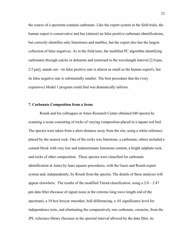
7. Carbonate Composition from a Scene

Roush and his colleagues at Ames Research Center obtained 640 spectra by

scanning a scene consisting of rocks of varying composition placed in a square soil bed.

The spectra were taken from a short distance away from the site, using a white reference

placed by the nearest rock. One of the rocks was limestone, a carbonate; others included a

cement block with very low and indeterminate limestone content, a bright sulphate rock,

and rocks of other composition. These spectra were classified for carbonate

identification at Ames by least squares procedures, with the Gazis and Roush expert

system and, independently, by Roush from the spectra. The details of these analyses will

appear elsewhere. The results of the modified Tetrad classification, using a 2.0 – 2.47

µm data filter (because of signal noise at the extreme long wave length end of the

spectrum), a 10 box boxcar smoother, hull differencing, a .01 significance level for

independence tests, and eliminating the comparatively rare carbonate, cerussite, from the

JPL reference library (because in the spectral interval allowed by the data filter, its

24

spectrum matches a sulphate) is shown in figure 1. The white rock in the upper right hand

corner is limestone.

Figure 1. Identification of pixels containing carbonates (C) and not containing carbonates (.) in a 20 x 32 pixel scene using the modified PC algorithm. For details, see text.

8. Experiments with Variable White Reference Location

Because the power spectrum of the sun varies with place and time, reflectance

spectra require comparison of the reflected light from a surface with that reflected from a

white reference surface. In laboratory studies, and in the laboratory and field studies so

far reported here, the reference is placed at or near the target sample. But remote sensing

requires that the white reference be near the spectroscope and remote from the target. We

have been able to find no study of the accuracy of deconvolution algorithms in this

deployment.

25

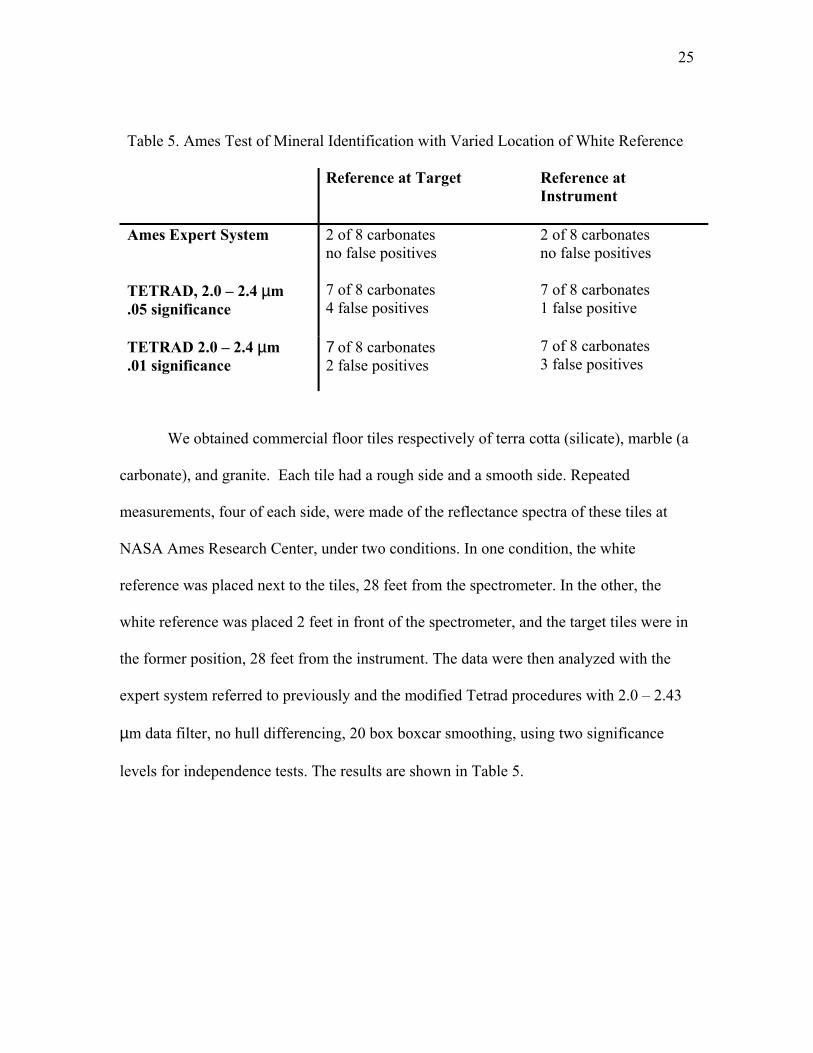
Table 5. Ames Test of Mineral Identification with Varied Location of White Reference Reference at Target

Reference at Instrument

Ames Expert System

2 of 8 carbonates no false positives

2 of 8 carbonates no false positives

TETRAD, 2.0 – 2.4 µm .05 significance

7 of 8 carbonates 4 false positives

7 of 8 carbonates 1 false positive

TETRAD 2.0 – 2.4 µm .01 significance

7 of 8 carbonates 2 false positives

7 of 8 carbonates 3 false positives

We obtained commercial floor tiles respectively of terra cotta (silicate), marble (a

carbonate), and granite. Each tile had a rough side and a smooth side. Repeated

measurements, four of each side, were made of the reflectance spectra of these tiles at

NASA Ames Research Center, under two conditions. In one condition, the white

reference was placed next to the tiles, 28 feet from the spectrometer. In the other, the

white reference was placed 2 feet in front of the spectrometer, and the target tiles were in

the former position, 28 feet from the instrument. The data were then analyzed with the

expert system referred to previously and the modified Tetrad procedures with 2.0 – 2.43

µm data filter, no hull differencing, 20 box boxcar smoothing, using two significance

levels for independence tests. The results are shown in Table 5.

26

9. Other Mineral Classes: A Human Expert Baseline and a John Henry Experiment

Many other minerals or mineral classes other than carbonates are of scientific

interest or of interest in terrestrial or Martian exploration. To investigate whether

automated procedures can approximate human expertise for other mineral classes, we

obtained an experimental human expert baseline and compared it with the performance of

the modified Tetrad program with no data filter.

Roush examined 191 JHU spectra stripped of identifiers and attempted to

determine, for each of the 17 JPL mineral classes, which classes were present in the JHU

source. He had unlimited time and was free to use any reference works or computer aids

he wished. In the event he spent about 12 hours on the task over 4 days. The modified PC

algorithm was then run on the same spectra, using the entire 0.4 µm – 2.5 µm spectrum,

hull differenced, at 0.05 significance for independence tests, and outputting any of the 17

JPL classes if a representative of that class was found for a sample. For eight of the

seventeen JPL mineral classes, no representative, or no more than two representatives,

were present in the JHU library, and for those classes the experiment is of no

significance. The results are shown graphically in Figures 2a and 2b.

27

Probability(Mineral Class = X when TETRAD Says Mineral Class = X). Probability(TETRAD Says Mineral Class = X when Mineral Class = X)

0.00

0.20

0.40

0.60

0.80

1.00

tectos

ilicate

s

phyllo

silica

tes

carbo

nates

inosili

cates

oxide

s

neso

silica

tes

phos

phate

s

sulfid

es

borat

es

cyclo

silica

tes

elemen

ts

halid

es

hydro

xides

soros

ilicate

s

sulph

ates

tungs

tates

arsen

ates

Perc

ent

P(Truth | Tetrad) P(Tetrad | Truth)

Figure 2a. See text.

Probability(Mineral Class = X when Expert Says Mineral Class = X)Probability(Expert Says Mineral Class = X when Mineral Class = X)

0.00

0.20

0.40

0.60

0.80

1.00

tectos

ilicate

s

carbo

nates

neso

silica

tes

phyllo

silica

tes

inosili

cates

oxide

s

elemen

ts

sulfid

es

cyclo

ilicate

s

halid

es

hydro

xides

sulph

ates

arsen

ates

borat

es

phos

phate

s

soros

ilicate

s

tungs

tates

Perc

ent

P(Truth | Expert) P(Expert | Truth)

s

Figure 2b. See text.

28

For tectosilicates, phyllosilicates and inosilicates the positive identifications of the human

expert have significant reliability, and can be approximated (with more false positives

and fewer false negatives) by the modified PC algorithm. We have reason to hope,

therefore, that subclasses of these mineral groups can be distinguished, and informative

spectral regions found, for which the machine procedures will be useful. The problem is

to find informative data filters for each class, if they exist.

10. Automated Construction of Data Filters

Moody et al. (2001) describe two methods for locating data filters for a given

mineral class. One procedure bins the intensities of library spectra at each frequency and

computes the information about the given class at each spectral interval. A second

procedure partitions the 4.0 – 2.5 mm spectral region into intervals and codes each

interval as an allele value (present or absent) in a genetic algorithm, using the modified

tetrad algorithm to evaluate fitness.

The information algorithm is sensitive to the number of bins used, and the genetic

algorithm is sensitive to the number of elements of the partition—the number of genes—

used. Best results in the experiments were obtained with a genetic algorithm with ten

genes. An interval for carbonates corresponding closely to the 2.0 – 2.5 mm region was

found, and reasonably well-defined intervals were also found for inosilicates. Other

mineral classes and subclasses have not been explored.

29

11. Discussion

In less formal experiments we have used the JPL library as a training set and the

JHU library as a test set to explore a number of other approaches to automated mineral

classification from reflectance spectra, with little success. Kohenen self-organizing maps

and AutoClass yield interesting classifications of the JPL spectra, but they generally do

not correspond to standard mineral classifications of geological interest. The problem of

identifying mineral composition from reflectance spectra seems as if it could fruitfully be

treated by neural net techniques, and that was our initial approach. In 1996 we generated

training data for a network with four hidden nodes by taking random linear combinations

of JPL spectra and we testing the trained network on JHU data. JPL investigators have

subsequently used a similar approach. We trained networks for carbonate identification

but found that the networks did not perform well if the test data contained significant

fractions of minerals not in the training set. A further problem is that in reality the

reflectance spectra of rocks, soils and other materials are not in general linear or even

additive functions of the spectra of their component minerals, and such training

procedures therefore lack realistic training sets.

We have attempted carbonate identification with two Support Vector Machine

programs available online (“MySvm” and “SvmLight”). Treating labels as continuous

produced some promising results superficially similar to those reported here. However,

with labels treated as discrete, as they are treated for the algorithms reported above,

neither program converged at all, no matter which general purpose kernel was used.

It may well be that boosting techniques, or carefully chosen kernels for Support

Vector Machines, or something else altogether that we have not considered, will improve

30

on the results reported here for the modified PC algorithm with appropriate data filters,

but for the present the modified PC algorithm seems to be the best available procedure

for the identification of carbonate content in minerals and perhaps for the identification of

other mineral class content as well. The algorithm can be improved in various ways, for

example by resolving ambiguities—such as that between cerussite and certain

sulphates—within the range admitted by a data filter by comparing spectral regions

excluded by the data filter.

Executables and source code for all of the algorithms described in this paper,

except the Gazis-Roush expert system and proprietary Model 1 algorithms, can be

downloaded from http://www.phil.cmu.edu/rockspec. Data sets described in this paper

can be downloaded from the same location.

31

References.

Gaffey, S.J. (1987). Spectral reflectance of carbonate minerals in the visible and near-

infrared (0.35-2.55 µm): anhydrous carbonate minerals. J. Geophys. Res., 92,

1429-1440.

Gazis, P. R. and Roush, T. (2001). Autonomous identification of carbonates using near-

IR reflectance spectra during the February 1999 Marsokhod field tests. J.

Geophys. Res. Vol. 106, No. E4.

Glymour, C. and Cooper, G. (1999). Causation, Computation and Discovery.

MIT/AAAI Press.

Grove, C. I., Hook, S. J., and Paylor II, E. D. 1992. Laboratory reflectance spectra of 160

minerals, 0.4 to 2.5 micrometers. JPL-Publication 92-2.

Hapke, B. (1993). Theory of Reflectance and Emittance Spectroscopy. New York:

Cambridge Univ. Press.

Johnson, Jeffrey R. and 11 others (2001). Geological characterization of remote field

sites using visible and infrared spectroscopy: Results from the 1999 Marsokhod

field test. J. Geophys. Res. Vol. 106, No. E4.

Moody, J., Silva, R., Vanderwaart, J. and Glymour, C. (2001). Data filtering for

automatic classification of rocks from reflectance spectra. Proceedings of the 7th

ACM SIGKDD Conference on Knowledge Discovery and Data Mining, p. 347-

352. San Francisco, CA: ACM Press.

Pearl, J. (1988). Probabilistic Reasoning in Intelligent Systems. San Mateo: Morgan and

Freeman.

32

Pieters, C.M. and P.A.J. Englert, Eds. (1993). Remote Geochemical Analysis: Elemental

and Mineralogical Composition. New York: Cambridge Univ. Press.

Scheines, R., Spirtes, P., Glymour, C. and Meek C. (1994). TETRAD II. Laurence

Erlbaum Publishers.

Spirtes, P., Glymour C. and Scheines, R. (1993). Causation, Prediction and Search. New

York: MIT Press (Springer Verlag Lecture Notes in Statistics).

Spirtes, P., Glymour C. and Scheines, R. (2000). Causation, Prediction and Search,

Second Edition. New York: MIT Press (Springer Verlag Lecture Notes in

Statistics).

Stoker, C.R., N. Cabrol, T. Roush, J. Moersch, et al. (2001). The 1999 Marsokhod Rover

mission simulation at Silver Lake California: mission overview, data sets, and

summary of results. J. Geophys. Res., v. 106, p. 7639-7663.

33

Endnote

1 In order, the associations of the authors are: Department of Philosophy, Carnegie

Mellon University, Pittsburgh, PA (jdramsey@andrew.cmu.edu); NASA Ames Research

Center, Mountain View, CA (troush@mail.arc.nasa.gov); NASA Ames Research Center,

Mountain View, CA (pgazis@mail.arc.nasa.gov); Department of Philosophy, Carnegie

Mellon University, Pittsburgh, PA (ps7z@andrew.cmu.edu); Department of Philosophy

and Center for Automated Learning and Discovery, Carnegie Mellon University; and

Department of Philosophy, Carnegie Mellon University and Institute for Human and

Machine Cognition, University of West Florida (cg09@andrew.cmu.edu). Questions and

comments should be directed to the first or last authors. This research was supported by a

grant to the last author from the NASA Ames Research Center (Award Number NCC2-

1026) and the NASA AISRP program (Award Number NAG5-9309).

2 The spectral channels for the JPL library range in wavelength from 0.400 µm to 2.500

µm. They increase by 0.001 µm from 0.400 µm to 0.800 µm and then by 0.004 µm from

0.800 µm to 2.500 µm, for a total of 826 channels.

3 We thank Dawn Robinson and Ray Arvidson of Washington University for the

petrological analysis of this sample.

4 The JPL mineral library contains spectra for 160 different minerals, each of which is

measured at from one to three different powder grain sizes. Of these 160 minerals, 135

minerals are measured at the large grain size (125 – 500 µm). It is this set of 135 large

grain spectra which is used as a background library.

5 In this case, the number of variables is 135 and the sample size is equal to the number of

channels in the interval [2.0 µm, 2.5 µm] for the JPL library = 126.

34

6 The JHU spectral library contains many more spectra than just these 192 rock spectra,

including spectra for soils and plants, but our interest was just in the rock spectra. The

rock spectra were of six types: (1) solid igneous, (2) powdered igneous, (3) large grain

powdered metamorphic, (4) small gain powdered metamorphic, (5) large grain powdered

sedimentary, and (6) small grain powdered sedimentary.