Embed Size (px)
Citation preview
Automated Target Detection for Geophysical Applications
A Dissertation Presented
by
Uri Pe’er
to
The Department of Electrical and Computer Engineering
in partial fulfillment of the requirements
for the degree of
Doctor of Philosophy
in
Electrical Engineering
Northeastern University
Boston, Massachusetts
April 2017

To my wife Yifat, whose constant support made this work possible.
i

Contents
List of Figures iv
List of Tables vi
List of Acronyms vii
Acknowledgments viii
Abstract of the Dissertation ix
1 Introduction 11.1 Motivation . . . . . . . . . . . . . . . . . . . . . . . . . . . . . . . . . . . . . . . 11.2 Related Work . . . . . . . . . . . . . . . . . . . . . . . . . . . . . . . . . . . . . 21.3 Structure of This Work . . . . . . . . . . . . . . . . . . . . . . . . . . . . . . . . 5
2 Propagation Models of GPR Signals 62.1 Review of the Target Models . . . . . . . . . . . . . . . . . . . . . . . . . . . . . 6
2.1.1 Definitions and Problem Description . . . . . . . . . . . . . . . . . . . . . 72.1.2 Model Assumptions . . . . . . . . . . . . . . . . . . . . . . . . . . . . . 82.1.3 The system of equations for the full propagation model . . . . . . . . . . . 82.1.4 Approximation 1: Elevated, Mono-Static Model . . . . . . . . . . . . . . 112.1.5 Approximation 2: Bi-Static Model . . . . . . . . . . . . . . . . . . . . . . 112.1.6 Approximation 3: Modified Bi-Static Model . . . . . . . . . . . . . . . . 122.1.7 A Polynomial Approximation to the Bi-Static Model . . . . . . . . . . . . 142.1.8 The Naıve Model - Mono-Static, Ground Coupled System . . . . . . . . . 15
2.2 Selecting the Appropriate Physics-Based Model . . . . . . . . . . . . . . . . . . . 15
3 Locally Isolated Target Case 203.1 Target Detection Algorithm . . . . . . . . . . . . . . . . . . . . . . . . . . . . . . 21
3.1.1 Definitions and Terminology . . . . . . . . . . . . . . . . . . . . . . . . . 223.1.2 Summary of Detection Steps . . . . . . . . . . . . . . . . . . . . . . . . . 243.1.3 Example of the Intermediate Steps . . . . . . . . . . . . . . . . . . . . . . 253.1.4 Computational Load of the Algorithm . . . . . . . . . . . . . . . . . . . . 293.1.5 Relationship Between Taylor Expansion and Polynomial Regression . . . . 30
ii
3.2 Learning the Model Parameters From the Target . . . . . . . . . . . . . . . . . . . 323.3 Results . . . . . . . . . . . . . . . . . . . . . . . . . . . . . . . . . . . . . . . . . 333.4 Discussion . . . . . . . . . . . . . . . . . . . . . . . . . . . . . . . . . . . . . . . 36
4 Generalization of the Automated Target Detection Algorithm 374.1 Analyzing the Weakness of the Detection Algorithm . . . . . . . . . . . . . . . . 38
4.1.1 Multi Layered Medium . . . . . . . . . . . . . . . . . . . . . . . . . . . . 394.1.2 Multiple Targets . . . . . . . . . . . . . . . . . . . . . . . . . . . . . . . 40
4.2 Detection Algorithm, Re-Visited . . . . . . . . . . . . . . . . . . . . . . . . . . . 414.2.1 Analyzing a New Scan . . . . . . . . . . . . . . . . . . . . . . . . . . . . 424.2.2 Building Trajectories . . . . . . . . . . . . . . . . . . . . . . . . . . . . . 454.2.3 Utilizing Amplitude Information . . . . . . . . . . . . . . . . . . . . . . . 474.2.4 Obtaining the Model Parameters . . . . . . . . . . . . . . . . . . . . . . . 494.2.5 Sensitivity Analysis of the Model Parameters . . . . . . . . . . . . . . . . 50
4.3 Decision Making Stage . . . . . . . . . . . . . . . . . . . . . . . . . . . . . . . . 534.4 Results . . . . . . . . . . . . . . . . . . . . . . . . . . . . . . . . . . . . . . . . . 55
4.4.1 Testing the Algorithm . . . . . . . . . . . . . . . . . . . . . . . . . . . . 554.4.2 Performance of the Algorithm . . . . . . . . . . . . . . . . . . . . . . . . 584.4.3 Comparing the Algorithm Performance with That of a Single Class SVM . 59
5 Discussion and Future Research 625.1 Processing a New Scan . . . . . . . . . . . . . . . . . . . . . . . . . . . . . . . . 625.2 Processing the T and A Matrices . . . . . . . . . . . . . . . . . . . . . . . . . . . 635.3 Decision Making . . . . . . . . . . . . . . . . . . . . . . . . . . . . . . . . . . . 645.4 Additional topics for research . . . . . . . . . . . . . . . . . . . . . . . . . . . . . 64
6 Conclusion 65
A Calculating the Theoretical Curves 68
B Sensitivity Analysis of the Propagation Models 71B.1 Sensitivity of the Full Propagation Model to the Parameters . . . . . . . . . . . . . 72
B.1.1 Effect of Parameter Changing on the Curve Offset . . . . . . . . . . . . . 72B.1.2 Effect of Parameter Changing on the change of the curvature . . . . . . . . 75
B.2 Sensitivity of the Approximated Bi Static Propagation Model to the Parameters . . 76B.2.1 Analytical Analysis of the Sensitivity of the Model . . . . . . . . . . . . . 77B.2.2 Effect of Parameter Changing on the Curve Offset . . . . . . . . . . . . . 77B.2.3 Effect of Parameter Changing on the change of the curvature . . . . . . . . 80
Bibliography 83
iii

List of Figures
2.1 Ray Tracing schematics. A Bi-Static system is located at (x,g), and the target at (0,-h). 92.2 Ray Tracing schematics of the Modified BiStatic Model. A Bi-Static system is
located at (x,0), and the target at (0,-(h+R)). . . . . . . . . . . . . . . . . . . . . . 122.3 Example for model comparison - a target was placed in Styrofoam block at depth of
14.4 cm. . . . . . . . . . . . . . . . . . . . . . . . . . . . . . . . . . . . . . . . . 172.4 Example for model comparison - a target was placed in a concrete block with a
permittivity of 5.9. . . . . . . . . . . . . . . . . . . . . . . . . . . . . . . . . . . 182.5 Example for model comparison - a target was placed in a concrete block with a
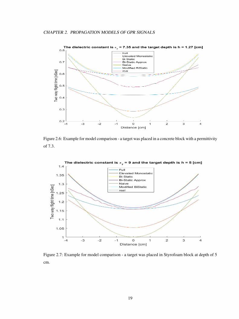
permittivity of 6.7. . . . . . . . . . . . . . . . . . . . . . . . . . . . . . . . . . . 182.6 Example for model comparison - a target was placed in a concrete block with a
permittivity of 7.3. . . . . . . . . . . . . . . . . . . . . . . . . . . . . . . . . . . 192.7 Example for model comparison - a target was placed in Styrofoam block at depth of
5 cm. . . . . . . . . . . . . . . . . . . . . . . . . . . . . . . . . . . . . . . . . . 19
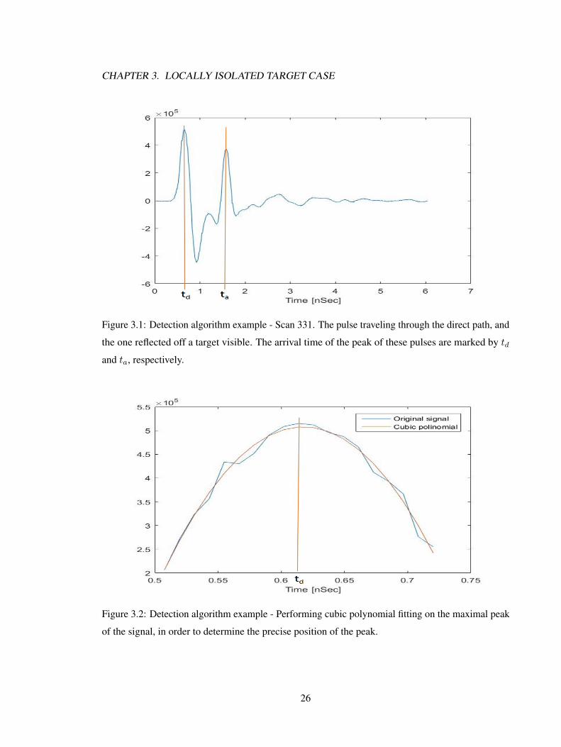
3.1 Detection algorithm example - Scan 331. The pulse traveling through the direct path,and the one reflected off a target visible. The arrival time of the peak of these pulsesare marked by td and ta, respectively. . . . . . . . . . . . . . . . . . . . . . . . . 26
3.2 Detection algorithm example - Performing cubic polynomial fitting on the maximalpeak of the signal, in order to determine the precise position of the peak. . . . . . . 26
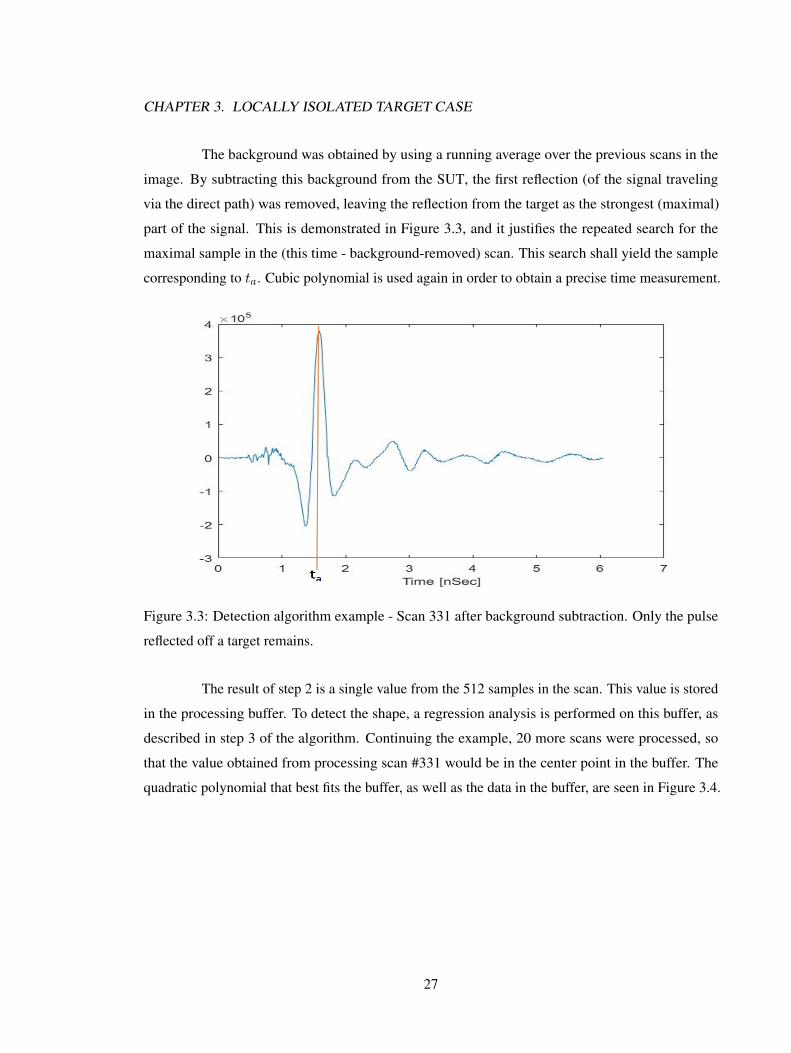
3.3 Detection algorithm example - Scan 331 after background subtraction. Only thepulse reflected off a target remains. . . . . . . . . . . . . . . . . . . . . . . . . . . 27
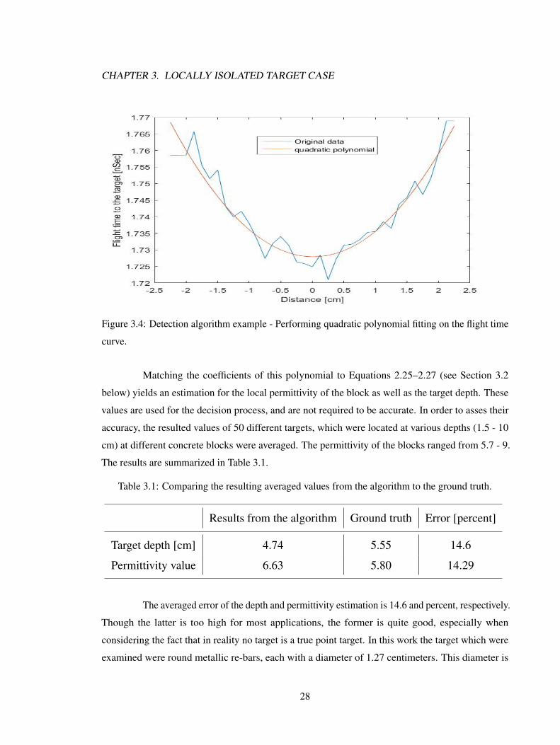
3.4 Detection algorithm example - Performing quadratic polynomial fitting on the flighttime curve. . . . . . . . . . . . . . . . . . . . . . . . . . . . . . . . . . . . . . . 28
3.5 Detection algorithm performance - Two targets block with permittivity of 5. Thealgorithm marked the detected scans. . . . . . . . . . . . . . . . . . . . . . . . . . 34
3.6 Detection algorithm performance - Six targets in depth ranging from 10 to 1.5 cm ina block with permittivity of 5.8. . . . . . . . . . . . . . . . . . . . . . . . . . . . 34
3.7 Detection algorithm performance - Six targets in depth ranging from 10 to 1.5 cm ina block with permittivity of 9. . . . . . . . . . . . . . . . . . . . . . . . . . . . . 35
3.8 Detection algorithm performance - A block with re-bars, located at depth of 10 cm.The block permittivity is 6. . . . . . . . . . . . . . . . . . . . . . . . . . . . . . . 35
4.1 Three Layered Medium. . . . . . . . . . . . . . . . . . . . . . . . . . . . . . . . 40
iv

4.2 Two mesh grids with three targets between them. . . . . . . . . . . . . . . . . . . 414.3 Analysis of a scan. The local extrema points are marks by orange X and are numbered
by the algorithm. . . . . . . . . . . . . . . . . . . . . . . . . . . . . . . . . . . . 444.4 The time of flight curve of a target before the trajectory building step. The jumps
from one peak to the next are clearly visible. . . . . . . . . . . . . . . . . . . . . . 454.5 The time of flight curve of a target after the trajectory building step. . . . . . . . . 474.6 The amplitude curve of a target after the trajectory building step. . . . . . . . . . . 484.7 Example of a single decision boundary that was created for the detection stage. . . 544.8 Block with crossing bars and tension cords. . . . . . . . . . . . . . . . . . . . . . 564.9 Block with Pan Decking. . . . . . . . . . . . . . . . . . . . . . . . . . . . . . . . 574.10 Block with PVC pipe above Re–bars. . . . . . . . . . . . . . . . . . . . . . . . . 584.11 Detection on the floor, Using Manually created decision rules for the detection stage. 604.12 Detection on the floor, using a single class SVM in the detection stage. . . . . . . . 61
A.1 Ray Tracing schematics. A transceiver is located at (y,-g), and the target at (0,h). . 69
B.1 Different Curves Produced by the Full Propagation Model for a target in differenttypes of medium. . . . . . . . . . . . . . . . . . . . . . . . . . . . . . . . . . . . 72
B.2 Different Curves Produced by the Full Propagation Model for a target in differentDepth. . . . . . . . . . . . . . . . . . . . . . . . . . . . . . . . . . . . . . . . . . 73
B.3 Different Shape of the Curves Produced by the Full Propagation Model for a targetin different types of medium. . . . . . . . . . . . . . . . . . . . . . . . . . . . . . 75
B.4 Different Shape of the Curves Produced by the Full Propagation Model for a targetin different Depth. . . . . . . . . . . . . . . . . . . . . . . . . . . . . . . . . . . . 76
B.5 Different Curves Produced by the Polynomial Approximation to the Bi Static Propa-gation Model for a target in different types of medium. . . . . . . . . . . . . . . . 78
B.6 Different Curves Produced by the Polynomial Approximation to the Bi Static Propa-gation Model for a target in different Depth. . . . . . . . . . . . . . . . . . . . . . 78
B.7 Different Shape of the Curves Produced by the Polynomial Approximation to the BiStatic Propagation Model for a target in different types of medium. . . . . . . . . . 80
B.8 Different Shape of the Curves Produced by the Polynomial Approximation to the BiStatic Propagation Model for a target in different Depth. . . . . . . . . . . . . . . 82
v

List of Tables
2.1 Averaged values for the two performance indices. . . . . . . . . . . . . . . . . . . 16
3.1 Comparing the resulting averaged values from the algorithm to the ground truth. . . 28
4.1 Final False detections. . . . . . . . . . . . . . . . . . . . . . . . . . . . . . . . . 59
B.1 Sensitivity analysis of the target depth on the resulting Curve offset in the Full Model. 73B.2 Sensitivity analysis of the medium’s permittivity on the resulting Curve offset in the
Full Model. . . . . . . . . . . . . . . . . . . . . . . . . . . . . . . . . . . . . . . 74B.3 Sensitivity analysis of the target depth on the resulting Curve offset in the Full Model. 79B.4 Sensitivity analysis of the medium’s permittivity on the resulting Curve offset in the
Approximated Bi Static Model. . . . . . . . . . . . . . . . . . . . . . . . . . . . . 79
vi

List of Acronyms
BP Band Pass In reference to filters, a Band Pass filter is a filter whose pass band contains a limitedrange of frequencies.
DCT Discrete Cosine Transform A Fourier-related transform similar to the discrete Fourier transform(DFT), but using only real numbers. The transformed signal is being expressed by sum ofcosine functions.
GPR Ground Penetrating Radar. An imaging device that works by emitting UWB signals andrecording the reflected echoes. Usually the transmitting signal is a non-modulated short pulse.
GSSI Geophysical Survey Systems, Inc. A GPR manufacturer. Situated in New Hampshire, USA.
IIR Infinite Impulse Response A type of linear filter, whose response to an impulse input does notnullify after a limited number of steps.
QoF Quality of Fit A performance index used to choose the best physical model which describesthe data. This is typically lp norm for some p.
RF Radio Frequency Electro-Magnetic wave frequencies that lie in the range extending from around3 kHz to 300 GHz.
UWB Ultra Wide Band. The FCC [1] defines UWB devise as “any device where the fractionalbandwidth is greater than 0.25 or occupies 1.5 GHz or more of spectrum. The formula proposedby the Commission for calculating fractional bandwidth is 2fH−fLfH+fL
where fH is the upperfrequency of the 10 dB emission point and fL is the lower frequency of the 10 dB emissionpoint.”
SNR Signal to Noise Ratio. The ratio of the power of the signal and the noise variance at a givensample. This is a performance metric, used in classic detection scheme to determine theperformance of a detection system.
SUT Scan Under Test. The scan for which a decision on the existence of target need to be made.
SVM Support Vector Machine. Supervised learning method. Invented by Vapnik [2] in 1995, is anefficient binary classifier. It find the optimal hyperplane that separates the two classes.
vii

Acknowledgments
I would like to thank several people who supported me in doing this work:First and foremost, Mr. Leonid Galinovsky (Geophysical Survey Systems, Inc. (GSSI)),
who made this work possible. His guidance drove me to ever perfect the algorithm, and make itapplicable for commercial use. If this work will revolutionize the field of GPR surveys, which I verymuch am hoping that it will, it will largely be thanks to him.
Dr. Roger Roberts (GSSI) and Dr. David Cist (GSSI) contributed a lot of their experiences.Whenever I would get stuck along the way, I could always count on them for fresh ideas and directionsthat I might have overlooked, and for that I am forever grateful.
My Advisor, Professor Jennifer Dy, who helped me organize my abstract thoughts intoa coherent algorithm, and stopped me when I was running too fast without explaining my stepsalong the way. Indeed, only by treading carefully was I able to understand when (and why) does mymethod not work - and what should be done to fix it.
And last but not least - to my wife, Yifat Pe’er, whose continual encouragement andconstant support gave me the strength to follow through this research.
viii
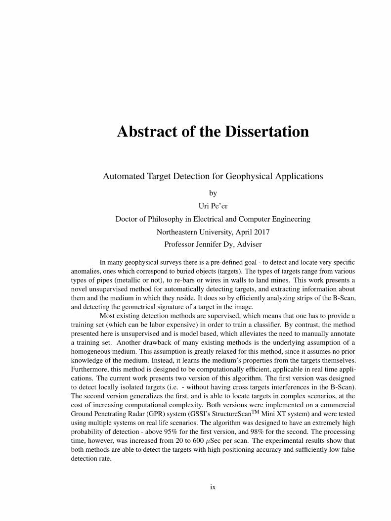
Abstract of the Dissertation
Automated Target Detection for Geophysical Applications
by
Uri Pe’er
Doctor of Philosophy in Electrical and Computer Engineering
Northeastern University, April 2017
Professor Jennifer Dy, Adviser
In many geophysical surveys there is a pre-defined goal - to detect and locate very specificanomalies, ones which correspond to buried objects (targets). The types of targets range from varioustypes of pipes (metallic or not), to re-bars or wires in walls to land mines. This work presents anovel unsupervised method for automatically detecting targets, and extracting information aboutthem and the medium in which they reside. It does so by efficiently analyzing strips of the B-Scan,and detecting the geometrical signature of a target in the image.
Most existing detection methods are supervised, which means that one has to provide atraining set (which can be labor expensive) in order to train a classifier. By contrast, the methodpresented here is unsupervised and is model based, which alleviates the need to manually annotatea training set. Another drawback of many existing methods is the underlying assumption of ahomogeneous medium. This assumption is greatly relaxed for this method, since it assumes no priorknowledge of the medium. Instead, it learns the medium’s properties from the targets themselves.Furthermore, this method is designed to be computationally efficient, applicable in real time appli-cations. The current work presents two version of this algorithm. The first version was designedto detect locally isolated targets (i.e. - without having cross targets interferences in the B-Scan).The second version generalizes the first, and is able to locate targets in complex scenarios, at thecost of increasing computational complexity. Both versions were implemented on a commercialGround Penetrating Radar (GPR) system (GSSI’s StructureScanTM Mini XT system) and were testedusing multiple systems on real life scenarios. The algorithm was designed to have an extremely highprobability of detection - above 95% for the first version, and 98% for the second. The processingtime, however, was increased from 20 to 600 µSec per scan. The experimental results show thatboth methods are able to detect the targets with high positioning accuracy and sufficiently low falsedetection rate.
ix
Chapter 1
Introduction
1.1 Motivation
Despite its name, a GPR system is not a RADAR system - it is missing a fundamental
component - target detection. Without detection, GPR is a sub-surface imaging system. To this date,
GPR manufacturers rely on skilled operator to analyze the resulting B-scan (also referred in this
work as the GPR image or the radargram), and to manually detect the anomalies that might be in it.
There are two main reasons for this missing capability: a lack of willingness to shoulder the liability
for detection (or mis-detection) among the manufacturers, and the fundamental problem of defining
what a target is.
The liability issue is an obvious one. GPR equipment is being used to locate many different
things: from cracks in ice sheets and dams to sewage or utility pipes to metallic re-bars. Failing to
detect one of the latter targets could cost a small fortune to a construction company, for example,
and might place people in real danger if one of the former targets is missed. For this reason, GPR
manufacturers sold their equipment to service providers - who then sold their expertise to those who
needed the information. However, it is the author’s personal belief that in this day and age, given that
a properly worded legal disclaimer is presented and signed by the user, this issue could be mitigated,
if not overcome completely. For this reason, this work will ignore the the legal issues that might be
involved. It does mean that when coming to design an algorithm which will be able to automatically
detect targets, it has to have a very high probability of detection, probably at the price of having a
high false detection rate.
GPR is a versatile tool, used to detect many things. It works by emitting a Radio Frequency
(RF) signal, and recording the reflected echoes. These echoes will be refracted by discontinuities
1
CHAPTER 1. INTRODUCTION
in the permittivity of the medium through which the signal is traveling. Discontinuities could be
caused by many factors, but the discontinuities of interest to the vast majority of GPR users are those
which originate from having a material which is different than its surrounding. Generally, these could
be classified into two families: discontinuities (anomalies) which are small relative to the scanned
distance, and discontinuities that are not. The former anomalies will be referred to as targets, and
this work will focus on attempting to detect and locate them in real time. The latter are layers in the
medium. Examples for targets include mines in the ground, re–bars and PVC pipes in concrete or
sewage/utility pipes/tunnels in the ground. In these cases, typically the users are would primarily
like to detect and locate the targets. Additional information of interest might include the size of the
targets and the material from which they are made of (determining whether an object is metallic or air
filled, for example). Examples for layers of interest would be asphalt layer on top of a packed gravel
layer in a paved road, and ice sheets on top of a river or a pond. In these examples, the required data
is typically the layers’ thickness and their permittivity.
This work focuses on detecting targets. This family of anomalies is wide enough to be of
interest to many of the current GPR users, and indeed, if a good enough detection method for these
targets exists - might alleviate the need for skilled GPR operator to analyze the image in order to find
these targets. Automatic target detection will result in making the data more accessible and easier for
interpretation, and this in turn might lead to more people who will use the system.
1.2 Related Work
GPR operates by emitting (“firing”) an Ultra Wide Band (UWB) signal, recording the
echoes and then being moved to a different location and starting again. The echoes from a single
signal form an A-scan. Collection of A-scans form the B-scan, that is the resultant GPR image.
Numerous works were conducted on understanding the signal as it travels in the ground. Richard
Yelf [3] and Stanley Radzevicius [4], for example, discuss the subject of finding the true time zero in
the A-scans. This time zero is the precise moment in which the energy was emitted by the system,
and hence it is the reference to the measurements of the time in which the signal was received after
its round trip to the target and back. Since the system can only sample the received signal, finding
the precise timing of transmission is non–trivial. It is crucial, however, for depth and permittivity
calculations. This work follows Yelf’s approach. In his method, the system is placed at a known
height above a metal plate reflector. Since the height is known, and the propagation speed in the
medium (which is air, making it the speed of light) is known, the expected (two way) flight time
2
CHAPTER 1. INTRODUCTION
of the signal could be calculated. By comparing the expected time to the measured, one can back
calculate time zero.
GPR is a versatile tool, and its images are used to detect a wide range of sub-surface
anomalies. Many studies were performed on detecting different type of anomalies: mine detection
( [5–8]) sinkholes [9], subterranean voids and tunnel detection [10, 11], buried utilities [12] cracks
in ice sheets [13]) as well as for bridges and roads assessment [14]. The vast majority of detection
methods involve some pre-processing stage (for example: Qin et Al. [10] used Discrete Cosine
Transform (DCT) on the image) followed by a classifier (usually Support Vector Machine (SVM) [15]
or neural network [16]). These methods, however, are computationally intensive, rendering them
unsuitable for real time decision making. In addition they need a training set to train the classifier -
which means that the datagram needs to be manually annotated to let the classifier know where the
targets in the training set are. This work presents a model based detection scheme which mitigates the
above shortcomings - being computationally efficient and minimizing the need for expert assistance
in the initial (training) stage. Another contribution is its ability to learn the model parameters - target
depth and dielectric constant - from the targets.
A point target creates a distinct shape (a hyperbola) in the datagram. This fact is being
used extensively in geophysical data processing, such as the various types of migration and move out
analysis [17], [18], as well as recent works which combined compressive sensing with GPR [19], [20].
Radzecius [4], Al-Naumi et al. [12] and Kang et al. [21] have presented simple bi-static model which
produces this shape. Khan et al. [7] uses the more accurate model than the bi-static one. Their model
incorporated some antenna distance off the ground - but ignored the fact that introducing a layer of air
above the medium will bend the energy rays as they pass from one layer to another. Gurbuz [22], [20]
uses the same model as Khan et al., but takes into account this bending. Martens et al. [23] presented
an interesting variation of the basic model, incorporating knowledge of the targets’ diameter. In
practice, however, it turned out that their model does not describe the data well - probably due to
the low ratio of the target size to the system’ wavelength. This shall be explored and elaborated in
Section 2.2.
Notable previous works are the works of Martens et al. [23], Wang et al. [24] and Pasolli et
al. [25] and Lee et al. [18]. These works do not relay on expert knowledge of the current medium’
properties (i.e. dielectric constant) but rather attempt to learn it from the data itself. However, their
pre-processing stage is computationally intensive (template matching for Wang et al., histogram
calculation of the entire image, in order to get the optimal thresholding value in Pasolli et al.). The
method proposed by Martens et al. could possibly be adapted to a real time algorithm, though their
3
CHAPTER 1. INTRODUCTION
current runtime was measured in minutes for a full B-Scan, as compared to few milliseconds for that
the algorithm presented in this work would require. Three other notable differences between those
works and the one presented here are the detection accuracy (the ability to pin-point the location of the
target), detection performance (as measured both in the probability of detection and false detection
rate in real field data) and the number of data sets used to calculate the detection performance. For
example, Pasolli et al. did not use a single field data file, but rather relied on a simulator to show
their performance. Even so, they reported a probability of detection of 62%, with no mention of the
number of false detections. Wang et al. showed a single file (albeit a long one) but do not mention
the performance of their algorithm at all. Martens et al., in contrast, did an extensive study of the
performance of their algorithm, and report a probability of detection which ranges from 72% to 92%
with some false detection. However, many of the detections were inaccurate (wrong sample was
chosen for target location) which reduces the overall performance of the algorithm. The algorithm
proposed in this work showed a probability of detection greater than 95.3%. In 50 different data sets,
collected by GSSI’s StructureScanTM Mini XT system, only 8 occurrences of false detections were
observed, as shall be described extensively in Section 3.3. Since those numbers were insufficient for
a commercial system, a second version of the algorithm was developed. Using 361 different data sets,
the probability of detection was shown to be 98.65%. This came at the price of increasing the run
time of the algorithm (from 20 to 600 µSec) and increasing the false detection rate. This is described
in Section 4.4.
4
CHAPTER 1. INTRODUCTION
1.3 Structure of This Work
The current work relies on the shape (hyperbola) created by point targets for detection. It
analyzes the GPR image to locate this shape and compare it to the expected, theoretical shape. The
first part of the work will focus on finding the best physical model that describes the true shape of the
target. Review of the different propagation models is covered in Chapter 2, as well as comparison
to the actual data collected by a GPR system. A detailed explanation of how this comparison was
carried out is found on Appendix A. This comparison will allow us to select the optimal physics
based model to be used later in the detection algorithm. Appendix B completes the analysis by
presenting a sensitivity analysis of that model.
The model is used in Chapter 3 to create a simple and effective target detection algorithm,
which is suited for real time applications and works well in most of the cases. Its shortcoming, how-
ever, are the fact that it assumes a simple enough scenario - a single target in a locally homogeneous
medium. Chapter 4 will remove those assumptions and present a method to generalize the algorithm
to more complex (and more realistic) scenarios - where multiple layers and targets interfere with
one another. It does so by modifying the pre-processing stage and the decision making stage - while
retaining the core idea of the first algorithm - that of comparing the collected data to an expected,
theoretical curve.
5
Chapter 2
Propagation Models of GPR Signals
The propagation model which will be used throughout the work shall be developed in
this chapter. It shall be used to predict the geometric shape that a target is expected to produce on
the datagram (B-Scan). The method for efficiently detect this shape will be described in the next
chapter. This chapter is organized as follows: Section 2.1 begins by detailing this model and clearly
stating the main assumptions underlying it. Since obtaining analytical solution to the model might be
challenging, three approximation to the model are derived. By comparing the predicted time-of-flight
that each model yields with data collected by a 2.6 GHz antenna, the optimal propagation model to
be used in this work is chosen in Section 2.2.
2.1 Review of the Target Models
A model-based approach was used in this work to target detection. This section provides
details of the theoretical model used. The terminology and definitions, used by the various propagation
models are presented in Section 2.1.1. The assumptions which the model is based upon are clearly
and explicitly stated in Section 2.1.2. The system of equations which mathematically describes the
full propagation model are presented in Section 2.1.3. This system is a set of non-linear equations.
Section 2.1.4, and Section 2.1.5 provide two alternative approximations to the full propagation
model – a mono-static and bi-static solution, respectively. Another approximation is provided in
Section 2.1.7 – a polynomial approximation to the bi-static solution. By equating the coefficients of
this polynomial with those obtained with a regression analysis, the detection method will be able to
efficiently determine the parameters of the model - the (unknown) target depth and the permittivity of
the bulk medium in the neighborhood above the target. For completeness, two of the approximations,
6

CHAPTER 2. PROPAGATION MODELS OF GPR SIGNALS
explored in Sections 2.1.4 and 2.1.5, are combined to yield to simplest propagation model, described
in Section 2.1.8. Indeed, it is this simplified model that one finds in most of the geophysical literature.
2.1.1 Definitions and Problem Description
The creation of the curve (the synthetic target) will be described in this section as well
as the variables and definitions used by the theoretical models which will be presented in the next
sections. By comparing the curves, created by the theoretical target model with data collected from a
GPR device, the best model could be chosen.
This work uses the following terminology and definitions:
• GPR/Imaging System - An imaging system is transmitting signals every dx meters. This
imaging system has a spatial separation of 2∆[m] between the transmitter and the receiver,
and an elevation (sometime referred as “air gap”) of g meters from the surface of the medium.
Possible sources for this air gap include the antenna housing (radom), and the sledge or the
cart in which the antenna lies. The magnitudes of the reflecting echoes are being recorded
at each location, and are used to generate the resulting images A and B-scans of the system.
Examples for these type of images are provided in Figure 3.1 (A-scan) and Figures 3.5 – 3.8
(B-scans).
• Medium - The half space in which the targets resides. This could be ice, drywall, concrete,
soil or any other material that might contains the target of interest. This work defines the
vertical (depth) axis as starting from the surface of the medium, with the positive direction
going into the medium.
• Target - In this work, targets are considered to be dimensionless (point targets). The origin of
the horizontal (distance) axis is defined to be the location of the target. The target is located h
[m] below the surface, making its coordinates (x, z) = (0, h) meters in the medium.
7
CHAPTER 2. PROPAGATION MODELS OF GPR SIGNALS
2.1.2 Model Assumptions
The assumptions listed below holds true regardless of the propagation model used.
1. The model is noise free.
2. The model assumes far field propagation.
3. The medium is locally homogeneous - it could be characterized as having a signal propagation
speed of vp(x), though the dependence on the system location x will be omitted in this work.
4. The medium has no special magnetic properties - the relative permeability Kr of the medium
is known, and equal to 1, throughout the (2 way) path.
5. The medium’ surface is flat as compared to the system wavelengths, in the small neighborhood
above the target.
6. The antennas are a point source and a point receiver.
7. The (2 way) propagation time t is known precisely.
It should be emphasized that this model deals with a single target. If multiple targets exists in the
medium, it is assumed that they are sufficiently separated spatially, so that only a single target could
be considered at a given moment.
The assumptions of locally homogeneous medium, combined with the assumption of non
magnetic medium, gives us the ability to use the dielectric constant εr of the medium is locally
constant throughout the (2 way) path:
εr =
(c
vp
)2
(2.1)
Where c is the speed of light in vacuum.
2.1.3 The system of equations for the full propagation model
Combining the definitions and assumptions above, one gets the following ray tracing
scheme for the Full Propagation Model, which will be described next. The signal is traveling from
the transmitter in the air mainly via the ray path r1, with an angle of Θ1 between the wavefront and
the surface, and gets to the target via the ray path r2 at an angle of Θ2. When the signal interacts
with the target, it is reflected off (and is refracted by) the target in all directions. The main energy
component that will eventually arrive at the receiver travels through the medium via path r3, with an
8

CHAPTER 2. PROPAGATION MODELS OF GPR SIGNALS
angle of Θ3 between the wavefront and the medium’s surface and arrives at the receiver mainly via
path r4. (See Figure 2.1 below).
Figure 2.1: Ray Tracing schematics. A Bi-Static system is located at (x,g), and the target at (0,-h).
The equations controlling the ray paths could be logically divided into three groups:
1. Equations which originate from the geometry of the problem:
From Figure 2.1 one can write the following set of equations:
r1 cos Θ1 = g (2.2)
r4 cos Θ4 = g (2.3)
r2 cos Θ2 = h (2.4)
r3 cos Θ3 = h (2.5)
r1 sin Θ1 + r2 sin Θ2 = x−∆ (2.6)
r3 sin Θ3 + r4 sin Θ4 = x+ ∆ (2.7)
9
CHAPTER 2. PROPAGATION MODELS OF GPR SIGNALS
2. Equations which originate from the boundary crossing:
Since far field propagation is assumed, one may use Snell’s law to obtain the following
connections between the angles:
sin Θ1
sin Θ2=
c
vp
∆= n (2.8)
sin Θ4
sin Θ3=
c
vp
∆= n (2.9)
Where n is the refraction coefficient of the medium. Using Equation 2.1 one get that n =√εr.
3. Time Measurement: The transmitted signal hits the target and is reflected back. The (two way)
travel time of the signal, along the path of r1 → r2 → r3 → r4 is given by:
r1 + r4
c+r2 + r3
vp= t(x, h,∆, g, vp) (2.10)
In this work t’s dependence on system location x, Bi static offset ∆, air gap g, target depth h
and signal velocity in the medium vp is dropped for brevity.
Equations 2.2 – 2.10 form a (non linear) system of 9 equations and 10 variables. Several
simplifying approximations to this system will be presented next. All of these approximations are
being used in practice, in different geophysical works. A numerical method for solving them is
presented in Appendix A. This method searches for the crossing point of the signal (from the air to the
ground or vice versa). The location of this crossing point is described by a fourth-order polynomial,
which is solved numerically. Once this point is found, the ray paths and the total time of flight are
calculated. A different method for calculating the time of flight for this model was presented by
Rappaport [26].
10
CHAPTER 2. PROPAGATION MODELS OF GPR SIGNALS
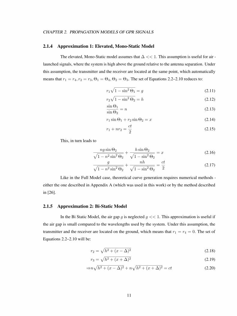
2.1.4 Approximation 1: Elevated, Mono-Static Model
The elevated, Mono-Static model assumes that ∆ << 1. This assumption is useful for air -
launched signals, where the system is high above the ground relative to the antenna separation. Under
this assumption, the transmitter and the receiver are located at the same point, which automatically
means that r1 = r4, r2 = r3,Θ1 = Θ4,Θ2 = Θ3. The set of Equations 2.2–2.10 reduces to:
r1
√1− sin2 Θ1 = g (2.11)
r2
√1− sin2 Θ2 = h (2.12)
sin Θ1
sin Θ2= n (2.13)
r1 sin Θ1 + r2 sin Θ2 = x (2.14)
r1 + nr2 =ct
2(2.15)
This, in turn leads to
ng sin Θ2√1− n2 sin2 Θ2
+h sin Θ2√1− sin2 Θ2
= x (2.16)
g√1− n2 sin2 Θ2
+nh√
1− sin2 Θ2
=ct
2(2.17)
Like in the Full Model case, theoretical curve generation requires numerical methods -
either the one described in Appendix A (which was used in this work) or by the method described
in [26].
2.1.5 Approximation 2: Bi-Static Model
In the Bi Static Model, the air gap g is neglected g << 1. This approximation is useful if
the air gap is small compared to the wavelengths used by the system. Under this assumption, the
transmitter and the receiver are located on the ground, which means that r1 = r4 = 0. The set of
Equations 2.2–2.10 will be:
r2 =√h2 + (x−∆)2 (2.18)
r3 =√h2 + (x+ ∆)2 (2.19)
⇒n√h2 + (x−∆)2 + n
√h2 + (x+ ∆)2 = ct (2.20)
11
CHAPTER 2. PROPAGATION MODELS OF GPR SIGNALS
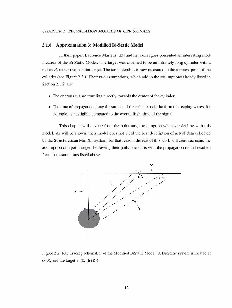
2.1.6 Approximation 3: Modified Bi-Static Model
In their paper, Laurence Martens [23] and her colleagues presented an interesting mod-
ification of the Bi Static Model: The target was assumed to be an infinitely long cylinder with a
radius R, rather than a point target. The target depth h is now measured to the topmost point of the
cylinder (see Figure 2.2 ). Their two assumptions, which add to the assumptions already listed in
Section 2.1.2, are:
• The energy rays are traveling directly towards the center of the cylinder.
• The time of propagation along the surface of the cylinder (via the form of creeping waves, for
example) is negligible compared to the overall flight time of the signal.
This chapter will deviate from the point target assumption whenever dealing with this
model. As will be shown, their model does not yield the best description of actual data collected
by the StructureScan MiniXT system; for that reason, the rest of this work will continue using the
assumption of a point target. Following their path, one starts with the propagation model resulted
from the assumptions listed above:
Figure 2.2: Ray Tracing schematics of the Modified BiStatic Model. A Bi-Static system is located at
(x,0), and the target at (0,-(h+R)).
12
CHAPTER 2. PROPAGATION MODELS OF GPR SIGNALS
From Figure 2.2 one get the following set of equations:
r1 =√
(h+R)2 + (x+ ∆)2 −R (2.21)
r2 =√
(h+R)2 + (x−∆)2 −R (2.22)
t =n
c(r1 + r2) (2.23)
This model is very interesting, because it allows the determination of the re–bar size from
the time of flight curve. Though not fully explored in the current work, the topic of re–bar size
assessment is of great importance for structural integrity and strength assessment of bridges, damns
and buildings. Re–bars tend to shrink in size due to corrosion, so having a non destructive method to
asses their size is very useful. Most existing methods [27–34] uses the amplitude of the signal in
order to determine the size of the re–bar. This has the limitation of amplitude variation from one
antenna to another, due to variabilities in the components of each antenna. Other methods (Utsi &
Utsi [27]) use ratio from cross polarize signal. This requires to double the number of channels. If the
proposed model is correct (i.e. low norm of the error when subtracting the theoretical curve from
the measured targets), then it means that the re–bar size could be inferred from the data directly
(possibly at the cost of having to assume the correct dielectric of the medium). This has several
advantages over the existing methods - for the time of flight of the GPR signal is significantly more
stable than the reflected amplitude, which allows for a more accurate estimation of the size of the
re–bar. In addition, no cross polarization information is needed in order to generate it, so compared
to the method which uses cross polarization, the number of transmitter-receiver pairs is halved.
Unfortunately, as will be shown in Section 2.2, This model does not describe the actual
data collected by the GPR system (GSSI StructureScan MiniXT system). This is probably due to
the fact that the ratio between the re–bar diameter (which, in the targets measured was 1.3 cm) to
the wavelength of the signal in the medium (which in a medium which has a dielectric constant of
εr ≈ 6 is about 5 cm) was too low.
13
CHAPTER 2. PROPAGATION MODELS OF GPR SIGNALS
2.1.7 A Polynomial Approximation to the Bi-Static Model
Since t(x) is a symmetric function with respect to the location of the system relative to
the target (t(x) = t(−x)), when calculating the McLauren polynomial which best describes it, only
even derivatives of it will be non-zero. Hence, obtain:
t(x) = t(0) + 0.5t′′(0)x2 +O(x4) (2.24)
The derivatives themselves are given by
ct(x) = n√h2 + (x−∆)2 + n
√h2 + (x+ ∆)2 (2.25)
⇒ t(0) =2n
c
√h2 + ∆2
ct′(x) =n(x−∆)√h2 + (x−∆)2
+n(x+ ∆)√h2 + (x+ ∆)2
(2.26)
⇒ t′(0) = 0
ct′′(x) =nh2
(h2 + (x−∆)2)3/2+
nh2
(h2 + (x+ ∆)2)3/2(2.27)
⇒ t′′(0) =2n
c
h2
(h2 + ∆2)3/2
ct(3)(x) =−3nh2(x−∆)
(h2 + (x−∆)2)5/2− 3nh2(x+ ∆)
(h2 + (x+ ∆)2)3/2(2.28)
⇒ t(3) = 0
Equations 2.28 , 2.26 prove Equation 2.24 and shows that a second order polynomial is
actually the third order approximation to the time of flight function, centered above the target. From
Equations 2.25 and 2.27 one gets that this parabolic function has to have positive offset (t(0) > 0)
and positive curvature (t′′(0) > 0). These facts will be exploited in the next chapters of this work.
14
CHAPTER 2. PROPAGATION MODELS OF GPR SIGNALS
2.1.8 The Naıve Model - Mono-Static, Ground Coupled System
Combine the two approximations to the Full Model - that of no elevation (g << 1) and
that of no bi-static offset (∆ << 1), one gets the wave propagation model which is commonly used
in the literature [17]. Under these assumptions, one has that r1 = r4 = 0 and r2 = r3, and the of
Equations 2.2–2.10 becomes:
t =2n√h2 + x2
c(2.29)
This approximation is very useful in practice, and is widely used. If the antenna is above
the target (t(0)), Equation 2.29 provides a linear relationship between the target depth and the
time-of-flight of the signal, and so the vertical scale of the radargram becomes linear. It also gives an
easy method of calibrating the scale: if one knows the true depth of a target, and measures the time
of flight at the apex (i.e. t(0)), the relative permittivity of the medium er = n2 is easily obtained
from Equation Equation 2.29.
2.2 Selecting the Appropriate Physics-Based Model
In order to choose the best physics-based model which describes the data collected by a
GPR system, several measurements were taken. 25 different datasets were obtained using a GPR
system - Geophysical Survey Systems, Inc. (GSSI) antenna, with a center frequency of 2.6 GHz. The
datasets were collected on various blocks of different material (in order to have a range of dielectric
constants). The material used were: Styrofoam block with a dielectric of εr = 1.07 (to test the
propagation model in extreme value), as well as several concrete slabs with dielectric values of
εr = 5.9, 6.7, 7.3 and 9.5, respectively. Re-bars at various (known) depths were placed inside these
blocks, at depths which ranged from 1.5 to 10 cm. The re–bar diameter was 1.27 cm. Each block
was scanned using several different GPR systems, and the targets were extracted from the resulting
B-Scan by tracking the maximal peak of the scan adjacent to the target location (total of 63 points per
target). A constant of toffset = 0.035 nanoseconds was added to the measured flight time of the signal
to accommodate for the time it takes for the signal to travel from the transmitter to the receiver.
The depth (and size) of the targets as well as the mediums’ permittivity were known
precisely enabling the generation of the theoretical curves, as each of the models, described in the
previous section, predicted. By comparing the data collected by the system to the different curves,
15
CHAPTER 2. PROPAGATION MODELS OF GPR SIGNALS
the optimal model will be selected. When comparing the data to a theoretical curve, two performance
metrics might be of interest:
• The shape of the curve - the l2 norm of the difference between the data points and the theoretical
curve. This metric will predict how well a given model describes the overall shape of a target.
• The difference at the apex (minimal point) - this difference (absolute or in percentage) will
describe how well could a model determine the correct depth of a target (given the dielectric)
For each target and for each of the theoretical models explored in the previous sections,
the two metrics described above were calculated. In order to choose the best model that describes the
data, the results were averaged over the range of target depths and permittivity of the mediums. The
averaged results are presented in Table 2.1.
Table 2.1: Averaged values for the two performance indices.
Theoretical model l2 norm of the difference Absolute difference
of the minimal point [percent]
Full model 0.4044 3.3091
Elevated, Mono-static model 0.8623 21.2522
Bi-static model 0.328 5.577
Modified Bi-static model 0.3096 5.194
Polynomial approximation
to the Bi-static model 0.2923 5.577
Naıve model 1.0111 33.8417
The system which was used for data collection (GSSI’s Mini XT system) has wheels which
elevates it to 8 mm above the blocks. Its instantaneous bandwidth spans from 1.2 GHz to 3.8 GHz,
which means that (in the air) the shortest wavelength is approximately 7.8 cm - almost ten times
bigger than the air gap. This can explain the fact that the polynomial approximation to the Bi-Static
model outperformed the other models - with an average l2 norm of 0.2923. It should be noted that
if one is interested in the other performance metric - which model gives the best prediction for the
target depth, given the dielectric - one gets that the Full model outperforms the other models, as the
reader might expect. It is interesting to note that though the Modified Bi Static model uses more
information (the diameter of the target) than the other models, it does not out perform any other
16
CHAPTER 2. PROPAGATION MODELS OF GPR SIGNALS
models - not in predicting the target depth (via the location of the apex of the resulting shape) nor by
predicting the target’s shape (hyperbola).
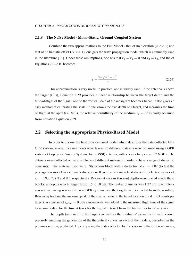
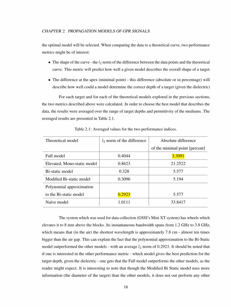
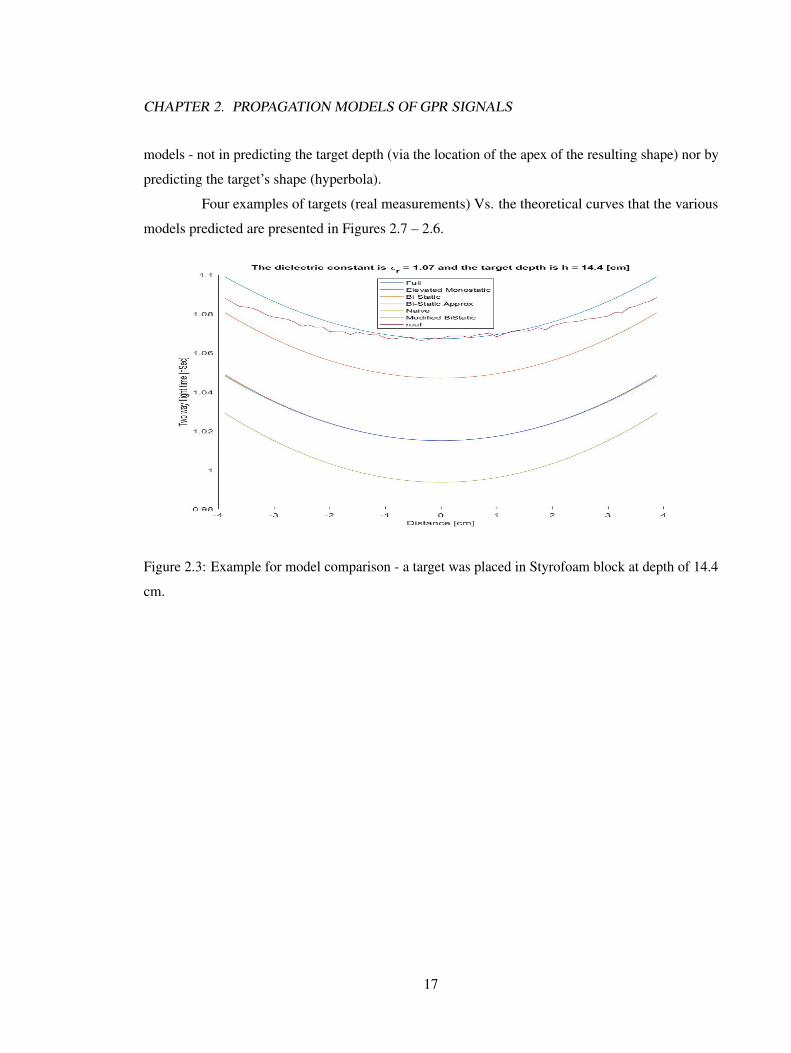
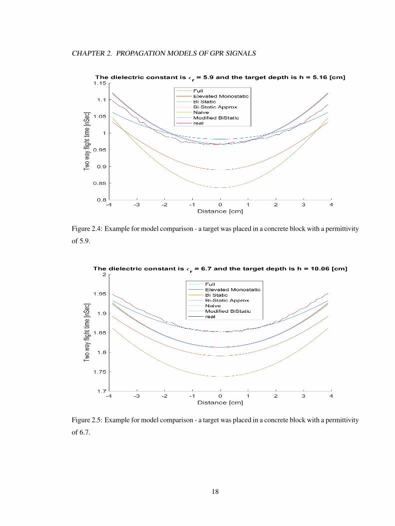
Four examples of targets (real measurements) Vs. the theoretical curves that the various
models predicted are presented in Figures 2.7 – 2.6.
Figure 2.3: Example for model comparison - a target was placed in Styrofoam block at depth of 14.4
cm.
17
CHAPTER 2. PROPAGATION MODELS OF GPR SIGNALS
Figure 2.4: Example for model comparison - a target was placed in a concrete block with a permittivity
of 5.9.
Figure 2.5: Example for model comparison - a target was placed in a concrete block with a permittivity
of 6.7.
18
CHAPTER 2. PROPAGATION MODELS OF GPR SIGNALS
Figure 2.6: Example for model comparison - a target was placed in a concrete block with a permittivity
of 7.3.
Figure 2.7: Example for model comparison - a target was placed in Styrofoam block at depth of 5
cm.
19
Chapter 3
Locally Isolated Target Case
The various propagation models used by different works were discussed in Chapter 2, as
well as the decision to use the Polynomial Approximation to the Bi-Static Model as the best model
(best in the sense that it describes the measurements with the least square error). A target detection
algorithm which utilizes this model will be described in this chapter. In order to use the model, the
algorithm will first obtain the data points of what is (potentially) the target. By comparing them to
the model (using regression analysis), the model parameters (i.e. the target depth h and the refraction
coefficient n) are being determined. By verifying that these parameters are within “normal” range, a
decision could be made regarding the existence of a target. This approach has several advantages
over existing target detection methods:
• It uses only local information. By nature, a target creates a local interference in the datagram.
While in some cases using information from different parts of the picture might assist the
decision (for example, to obtain statistics about the noise and DC levels in the B-Scan), one
cannot know in advance whether these parts of the image are indeed free from targets, layers
boundaries or any other inhomogeneity that might result in a strong signal, and will therefore
distort the noise estimation. In addition, using local information allows the algorithm to be
used in real time applications.
• It does not assume any pre-existing knowledge about the dielectric constant. As the previous
chapter showed, all the propagation model depends on the dielectric constant of the medium.
As appendix B shows, the selected model is sensitive to the dielectric. Any method that uses
a propagation model directly (for example - by performing migration, which is taking the
weighted sum of the pixels along the theoretical curve predicted by the model) has to assume
20
CHAPTER 3. LOCALLY ISOLATED TARGET CASE
the pre-knowledge of the permittivity of the medium. It is possible to asses it from the surface
reflection, but this estimation is not very accurate. In the case of multiple layers (a subject
which will be discussed in the next chapter) the estimation error of the dielectric constant of
the deeper layer is too big to be of any practical use.
This chapter is organized as follows: The proposed algorithm is discussed in Section 3.1.
This method is composed of three stages: pre-processing, feature extraction, and target detection. In
the pre-processing stage polynomial regression is performed both as a filter - increasing the resulting
Signal to Noise Ratio (SNR) which improves the accuracy of the measurements - and as a method
for reducing the dimension of the problem, lowering the overall number of computations in the
following stages of the algorithm. The feature extraction stage again uses polynomial regression,
in order to obtain the first coefficients of the Taylor’s series of the pulses’ flight time function. By
matching these coefficients to the theoretical model and using the Quality of Fit (QoF) as one of the
detection criteria, one easily determines whether the cell under test is the apex of a hyperbola or not.
Furthermore, from these coefficients one can learn the model parameters - the (locally averaged)
signal velocity in the medium and the target depth. Using this information, the decision of a target
existence is re-visited in order to rule out false detections. This step, in which the model parameters
are extracted from the targets, will be explored in Section 3.2. The overall results of the algorithm
will be presented in Section 3.3, with some discussion in Section 3.4.
3.1 Target Detection Algorithm
As was discussed in Section 2.1 and demonstrated in Section 2.2, the existence of a target
in the B-scan is visible through a distinct shape - a hyperbola. These shapes can be seen for example
in Figures 3.5 - 3.8. The location of a hyperbola’s apex and its aperture are being uniquely determined
by the model parameters - the target depth h and the permittivity of the medium εr.
The existence of a target creates an echo of the original pulse transmitted by the system
some time after the first arrival of the energy at the receiver - see Figure 3.1. In order to find
hyperbolas in the data, the pre-processing stage will locate these echoes in each of the scans, and
retain only this information. This produces a single dimensional function (instead of the full image)
- time of flight vs location. Since the influence of a target on this function diminishes the further
the system is from the target, the detection could be performed on localized observation of this
function - only the neighboring scans of the Scan Under Test (SUT) are important for the detection.
21
CHAPTER 3. LOCALLY ISOLATED TARGET CASE
This enables a real time algorithm, since the algorithm needs to retain only a limited amount of
information in order to perform the target detection.
The algorithm parameters are described in Section 3.1.1, as well as some trade-offs for
choosing their nominal values. The algorithm itself is detailed in Section 3.1.2: each new scan is
processed to determine the location of a possible echo. The timing of these locations are stacked
in a buffer, and a regression analysis for finding the best fit parabola is then performed. The model
parameters - target depth and propagation speed of the signal in the medium - are being determined
by equating the results of this analysis to the theoretical model. If these values are within range, a
detection is declared. A detailed example of this process is illustrated in Section 3.1.3.
A GPR system scan rate can be as high as a several KHz. This rate sets an upper bound on
the time frame upon which the algorithm has to run in order to be considered operating in real time.
This run time typically ranges from a few tens of microseconds up to a full millisecond. The addition
of the power consumed for the processing calls for the minimal number of computation required to
enable the desired performance of the algorithm. The computational complexity of the algorithm
shall be explored in Section 3.1.4, were a detailed review of the main mathematical tool (polynomial
regression) will be given. Since the algorithm equates the polynomial resulted from the regression to
the one resulting from a truncated Taylors’ series, the relationship between the two will be reviewed
in Section 3.1.5.
3.1.1 Definitions and Terminology
The following definitions are used throughout this section:
• M is the size of the buffer used for the time of flight function. This buffer can be viewed as a
sliding window over the time of flight function, as measured by the system. With each new
scan, this window will slide to the direction in which the system is currently moving, so the
corresponding curve could be created in real time.
• SUT - the scan in the middle of the buffer. Since the regression is performed on a full buffer,
increasing the buffer size M will cause longer delay (one will have to wait bM/2c scans to get
an answer).
• Out of the full scan, N samples are used at the pre-processing step to determine the precise
peak location.
• td - the arrival time of the direct coupling signal.
22
CHAPTER 3. LOCALLY ISOLATED TARGET CASE
• ta - the arrival time of the signal reflected from the target.
• toffset - a constant offset added to the difference between ta and td to compute the resulting time
of flight to the target. The theoretical models assume that the two way flight time is known
precisely. However, by analyzing the A-scan one can only deduce the time in which the signal
was received, and is lacking the knowledge of the time of transmission. The measured flight
time ta − td is a relative time - the true flight time to the target, minus the propagation time
from the transmitter to the receiver. In order to compare the measured and the predicted results,
one has to add the constant time of toffset, which is the propagation time of the signal from the
transmitter to the receiver. The value used in this work for toffset was found empirically by Dr.
Roger Roberts, in a similar method to the one described by Yelf [3]. This method was detailed
in Section 1.2, and it should be noted that this constant will be system dependent.
• tflight - the total time it took the signal to travel from the transmitter to the target, and back to
the receiver. It is given by
tflight = ta − td + toffset (3.1)
It should be noted that the measurement of td will depend on the material of the target.
Signals reflected off targets which have low dielectric constants (such as PVC pipes or air filled
cavities, for example) will have an opposite polarity compared to a signal reflected of a target with
a high dielectric constant (metallic re-bar, for example). This should be taken into account when
choosing the point of measurement (maximal or minimal peak).
There are several trade-offs when in choosing values for M and N . One of them - the
inherent delay of the detection algorithm - was already mentioned. Others include robustness of the
algorithm: the larger M , the more the algorithm is immune to a noisy single scan. The fact that the
“tails” of different hyperbolas created by different targets can cross makes detection harder. Similarly,
the larger N , the more the algorithm will be immune to noisy samples within a scan. As will be
shown, increasing M and N also increases the number of computations required at every step of the
algorithm.
23

CHAPTER 3. LOCALLY ISOLATED TARGET CASE
3.1.2 Summary of Detection Steps
The detection algorithm is summarized in Algorithm 1.
Algorithm 1 Summary of the detection algorithm.
1. Initialization step: Fill the buffer - go over the first M scans, and process them (as defined in
step 2 below).
2. Given a new scan, do the following :
(a) Determine the arrival time of the direct signal td (to be used as a reference):
i. Find the sample number n which corresponds to the maximal amplitude in the scan.
ii. Use polynomial regression to fit the N samples in the neighborhood of sample n.
iii. Determine the precise time, in which the polynomial reaches its maximal point.
(b) Subtract the background from the scan.
(c) Determine the arrival time of the target ta. This is done in a similar fashion to td, but is
performed on the modified scan (without the background).
(d) The (relative) time of flight for that scan is given by Equation 3.1.
(e) Store this value at the end of the buffer. This will discard the first value in the buffer and
will shift all other values one place closer to the beginning of the buffer.
3. Using quadratic regression procedure, find the best parabola which describes the data stored in
the buffer.
4. Determine whether the SUT is indeed a valid target.
5. Go back to step 2, and process a new scan.
24
CHAPTER 3. LOCALLY ISOLATED TARGET CASE
The decision which is performed in step 4 is based on several parameters:
• The QoF of the parabola. For example, the l2 or the l∞ norm of the fitting error.
• The location of the target (the apex of the parabola) has to be no more than half a scan interval
away from the SUT.
• By using feature extraction, obtain the model parameters (target depth and permittivity of the
medium - see Section 3.2); if these parameters are out of the expected range than the SUT
cannot contain a target.
This algorithm will be demonstrated in Section 3.1.3, and its computational load analyzed
in Section 3.1.4.
3.1.3 Example of the Intermediate Steps
To demonstrate how the algorithm process a given data set, a block with a permittivity of 6
was scanned using GSSI system with a center frequency of 2.6 GHz. This block has in it a mesh of
re-bars which are 10 cm apart. The resulted GPR image is presented in Figure 3.6.
The algorithm begins by processing each individual scan. For this example, scan number
331 was chosen (shown in Figure 3.1). This scan contains a target, which later will be detected by
the algorithm. This is displayed in Figure 3.2. The strongest part (maximal amplitude) of the scan is
the result of the signal traveling via the direct path, and arriving at the receiver without entering the
medium. For that reason, a simple search for the maximal value in the scan yields the sample which
corresponds to td. In order to get a more precise time of arrival of this signal, the algorithm uses
cubic polynomial with N = 15 (step 2ii in Algorithm 1).
25
CHAPTER 3. LOCALLY ISOLATED TARGET CASE
Figure 3.1: Detection algorithm example - Scan 331. The pulse traveling through the direct path, and
the one reflected off a target visible. The arrival time of the peak of these pulses are marked by td
and ta, respectively.
Figure 3.2: Detection algorithm example - Performing cubic polynomial fitting on the maximal peak
of the signal, in order to determine the precise position of the peak.
26
CHAPTER 3. LOCALLY ISOLATED TARGET CASE
The background was obtained by using a running average over the previous scans in the
image. By subtracting this background from the SUT, the first reflection (of the signal traveling
via the direct path) was removed, leaving the reflection from the target as the strongest (maximal)
part of the signal. This is demonstrated in Figure 3.3, and it justifies the repeated search for the
maximal sample in the (this time - background-removed) scan. This search shall yield the sample
corresponding to ta. Cubic polynomial is used again in order to obtain a precise time measurement.
Figure 3.3: Detection algorithm example - Scan 331 after background subtraction. Only the pulse
reflected off a target remains.
The result of step 2 is a single value from the 512 samples in the scan. This value is stored
in the processing buffer. To detect the shape, a regression analysis is performed on this buffer, as
described in step 3 of the algorithm. Continuing the example, 20 more scans were processed, so
that the value obtained from processing scan #331 would be in the center point in the buffer. The
quadratic polynomial that best fits the buffer, as well as the data in the buffer, are seen in Figure 3.4.
27
CHAPTER 3. LOCALLY ISOLATED TARGET CASE
Figure 3.4: Detection algorithm example - Performing quadratic polynomial fitting on the flight time
curve.
Matching the coefficients of this polynomial to Equations 2.25–2.27 (see Section 3.2
below) yields an estimation for the local permittivity of the block as well as the target depth. These
values are used for the decision process, and are not required to be accurate. In order to asses their
accuracy, the resulted values of 50 different targets, which were located at various depths (1.5 - 10
cm) at different concrete blocks were averaged. The permittivity of the blocks ranged from 5.7 - 9.
The results are summarized in Table 3.1.
Table 3.1: Comparing the resulting averaged values from the algorithm to the ground truth.
Results from the algorithm Ground truth Error [percent]
Target depth [cm] 4.74 5.55 14.6
Permittivity value 6.63 5.80 14.29
The averaged error of the depth and permittivity estimation is 14.6 and percent, respectively.
Though the latter is too high for most applications, the former is quite good, especially when
considering the fact that in reality no target is a true point target. In this work the target which were
examined were round metallic re-bars, each with a diameter of 1.27 centimeters. This diameter is
28
CHAPTER 3. LOCALLY ISOLATED TARGET CASE
greater than the absolute error (as measured in centimeters from the top most point of the targets).
It should be noted that the error in the estimation of both parameters is biased - the
predicted target depth and local permittivity were lower than the ground truth in all the targets tested
by the author. This presents the opportunity to decrease the (averaged) error by adding some fixed
percentage, so that the error will be unbiased. Since the estimation was used only for setting the
decision rules, this work did not pursue this route.
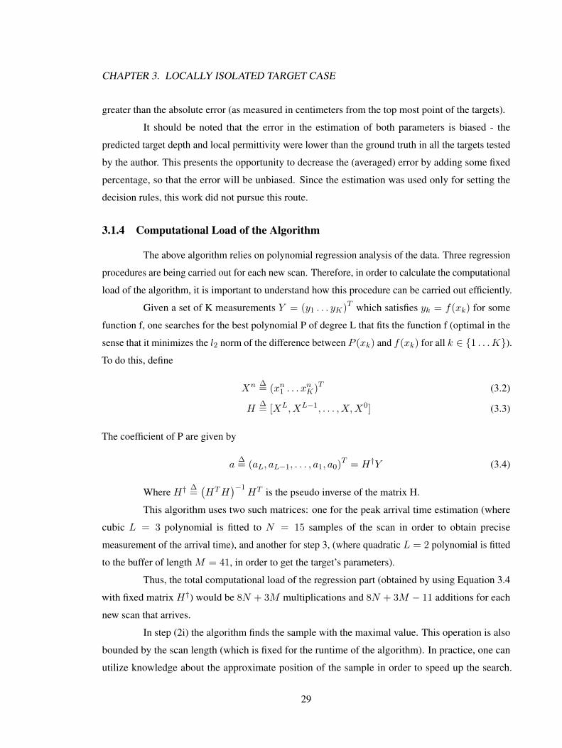
3.1.4 Computational Load of the Algorithm
The above algorithm relies on polynomial regression analysis of the data. Three regression
procedures are being carried out for each new scan. Therefore, in order to calculate the computational
load of the algorithm, it is important to understand how this procedure can be carried out efficiently.
Given a set of K measurements Y = (y1 . . . yK)T which satisfies yk = f(xk) for some
function f, one searches for the best polynomial P of degree L that fits the function f (optimal in the
sense that it minimizes the l2 norm of the difference between P (xk) and f(xk) for all k ∈ {1 . . .K}).To do this, define
Xn ∆= (xn1 . . . x
nK)T (3.2)
H∆= [XL, XL−1, . . . , X,X0] (3.3)
The coefficient of P are given by
a∆= (aL, aL−1, . . . , a1, a0)T = H†Y (3.4)
Where H† ∆=(HTH
)−1HT is the pseudo inverse of the matrix H.
This algorithm uses two such matrices: one for the peak arrival time estimation (where
cubic L = 3 polynomial is fitted to N = 15 samples of the scan in order to obtain precise
measurement of the arrival time), and another for step 3, (where quadratic L = 2 polynomial is fitted
to the buffer of length M = 41, in order to get the target’s parameters).
Thus, the total computational load of the regression part (obtained by using Equation 3.4
with fixed matrix H†) would be 8N + 3M multiplications and 8N + 3M − 11 additions for each
new scan that arrives.
In step (2i) the algorithm finds the sample with the maximal value. This operation is also
bounded by the scan length (which is fixed for the runtime of the algorithm). In practice, one can
utilize knowledge about the approximate position of the sample in order to speed up the search.
29
CHAPTER 3. LOCALLY ISOLATED TARGET CASE
Indeed, since the emission time te = td − toffset is stable from one scan to the next, one can use the
value from previous scans to narrow the search region for the new scan.
The above bound on the number of calculations required for each new scan, and the fact
that this bound is constant regardless of the number of scans, make the algorithm suitable for real
time applications.
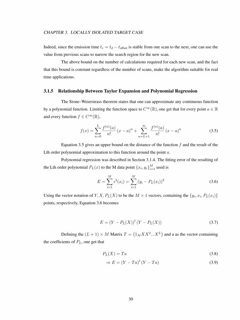
3.1.5 Relationship Between Taylor Expansion and Polynomial Regression
The Stone–Weierstrass theorem states that one can approximate any continuous function
by a polynomial function. Limiting the function space to C∞(R), one get that for every point a ∈ R
and every function f ∈ C∞(R),
f(x) =L∑n=0
f (n)(a)
n!(x− a)n +
∞∑n=L+1
f (n)(a)
n!(x− a)n (3.5)
Equation 3.5 gives an upper bound on the distance of the function f and the result of the
Lth order polynomial approximation to this function around the point a.
Polynomial regression was described in Section 3.1.4. The fitting error of the resulting of
the Lth order polynomial PL(x) to the M data point {xi, yi}Mi=1 used is
E =M∑i=1
ε2(xi) =M∑i=1
(yi − PL(xi))2 (3.6)
Using the vector notation of Y,X, PL(X) to be the M × 1 vectors, containing the {yi, xi, PL(xi)}points, respectively, Equation 3.6 becomes
E = (Y − PL(X))t (Y − PL(X)) (3.7)
Defining the (L + 1) ×M Matrix T =(1MXX
2...XL)
and a as the vector containing
the coefficients of PL, one get that
PL(X) = Ta (3.8)
⇒ E = (Y − Ta)t (Y − Ta) (3.9)
30
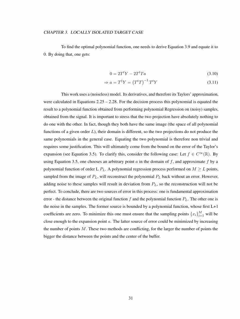
CHAPTER 3. LOCALLY ISOLATED TARGET CASE
To find the optimal polynomial function, one needs to derive Equation 3.9 and equate it to
0. By doing that, one gets:
0 = 2T tY − 2T tTa (3.10)
⇒ a = T †Y =(T tT
)−1T tY (3.11)
This work uses a (noiseless) model. Its derivatives, and therefore its Taylors’ approximation,
were calculated in Equations 2.25 – 2.28. For the decision process this polynomial is equated the
result to a polynomial function obtained from performing polynomial Regression on (noisy) samples,
obtained from the signal. It is important to stress that the two projection have absolutely nothing to
do one with the other. In fact, though they both have the same image (the space of all polynomial
functions of a given order L), their domain is different, so the two projections do not produce the
same polynomials in the general case. Equating the two polynomial is therefore non trivial and
requires some justification. This will ultimately come from the bound on the error of the Taylor’s
expansion (see Equation 3.5). To clarify this, consider the following case: Let f ∈ C∞(R). By
using Equation 3.5, one chooses an arbitrary point a in the domain of f , and approximate f by a
polynomial function of order L PL. A polynomial regression process performed on M ≥ L points,
sampled from the image of PL, will reconstruct the polynomial PL back without an error. However,
adding noise to these samples will result in deviation from PL, so the reconstruction will not be
perfect. To conclude, there are two sources of error in this process: one is fundamental approximation
error - the distance between the original function f and the polynomial function PL. The other one is
the noise in the samples. The former source is bounded by a polynomial function, whose first L+1
coefficients are zero. To minimize this one must ensure that the sampling points {xi}Mi=1 will be
close enough to the expansion point a. The latter source of error could be minimized by increasing
the number of points M . These two methods are conflicting, for the larger the number of points the
bigger the distance between the points and the center of the buffer.
31
CHAPTER 3. LOCALLY ISOLATED TARGET CASE
3.2 Learning the Model Parameters From the Target
Once a target has been detected, one naturally wishes to extract as much information
as possible about the target. This works reverses this logic: the decision of whether a given SUT
contains a target or not is based on the information extracted from it. This information are the
model parameters - the target depth h, and the signal’s speed of propagation in the medium vp in the
neighborhood of the target. Based on the model in use, one expects to obtain different curves from
different model parameters; This is demonstrated in Appendix B. Therefore, by matching the two
curves (one obtained from the quadratic regression which was described in step 3 of the algorithm,
and the other as obtained from the model) one is able to extract the desired parameters.
In general, this is an optimization problem and could easily be solved numerically. In one
special case, the approximation to the bi-static model, one can obtain an analytic solution to the curve
matching problem. This in turn guarantees that the matching is carried out with the minimum number
of computations, which allows the process to be performed in real time. For off-line calculations, the
use of a more accurate model would yield better results. Since it was shown that the approximated
bi-static model describes best (in terms of MMSE) the shape of the data, it was chosen for the initial
target detection stage. If a more precise estimation of the model parameters is required, then possibly
curve matching should be performed using a more accurate model on detected targets. To maintain
the efficiency of the overall algorithm, this stage will be performed only as a last step - on buffers
that are known to contain a target. The decision on the existence of a target in the buffer could then
be re-visited.
Step 3 of the algorithm produces a quadratic polynomial function t = a2x2 + a1x+ a0.
Equation 2.26 shows that a1 = 0. In general, this will not be true for the coefficients of the
polynomial, and therefore it needs to be centralized:
a2(x− a1
2a2)2 + a1(x− a1
2a2) + a0 = (3.12)
= a2x2 + a0 −
a21
4a2
32
CHAPTER 3. LOCALLY ISOLATED TARGET CASE
Using Equations (2.25 – 2.27), one finds that
a2 =1
2t′′(0) =
nh2
c (h2 + ∆2)3/2(3.13)
a0 −a2
1
4a2= t(0) =
2n
c
√h2 + ∆2 (3.14)
And by solving Equations 3.13 – 3.14 for h2 and n =√εr, one obtains the (approximated)
model parameters.
It should be noted that in order to avoid the inherent uncertainty of the pulse firing time
t0, one can use the second and fourth derivatives of the flight time, thus avoiding the need for toffset
which was introduced in Equation 3.1. This would require replacing the quadratic polynomial in step
3 with a fourth order one and match the resulting coefficients to the derivatives in a similar fashion to
the method that was described above.
3.3 Results
To asses the performance of the algorithm, 50 data sets with 278 targets were collected.
The targets were re-bars inserted into 6 inches blocks at known depths. The blocks were measured
independently in order to determine their (averaged) permittivity. Each block was scanned using a
GSSI system with a centered frequency of 2.6 GHz. Target depth ranged from 1.5 cm to 10 cm and
the permittivity of the blocks ranged from 1.07 to 14.
A total of 265 out of the 278 targets were located in those 50 different data sets, making the
probability of detection of these algorithm to pd = 0.953. In the entire collection of data sets, a total
of 8 scans were mis-classified as containing targets. Four examples of these data sets are presented in
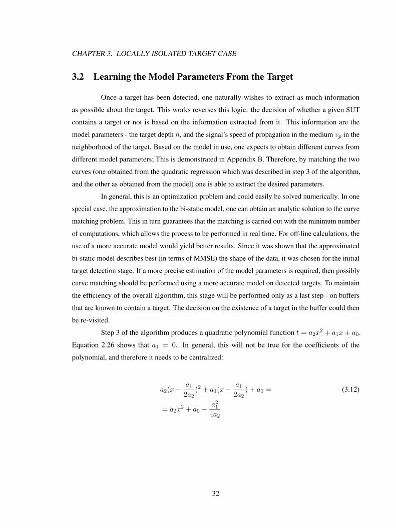
Figures 3.5 – 3.8. The location of the targets, as were found by the algorithm, are marked on the data.
33
CHAPTER 3. LOCALLY ISOLATED TARGET CASE
Figure 3.5: Detection algorithm performance - Two targets block with permittivity of 5. The
algorithm marked the detected scans.
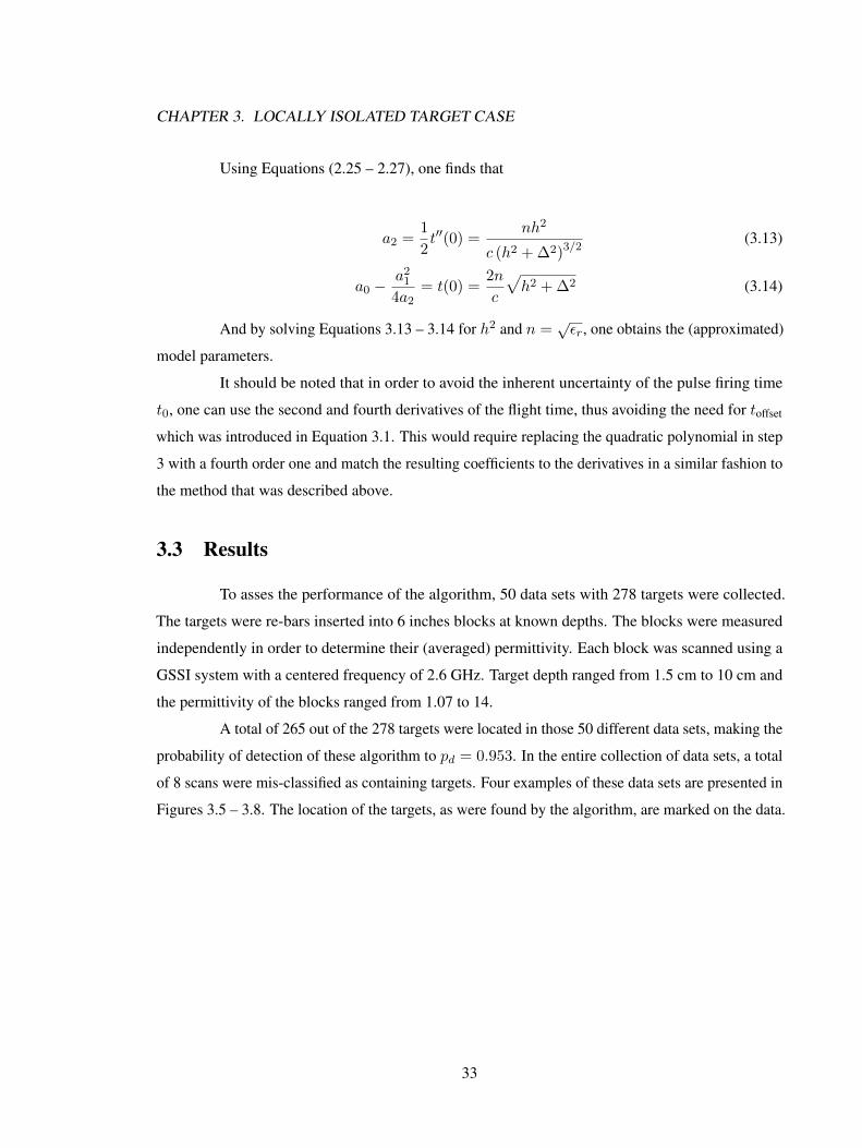
Figure 3.6: Detection algorithm performance - Six targets in depth ranging from 10 to 1.5 cm in a
block with permittivity of 5.8.
34
CHAPTER 3. LOCALLY ISOLATED TARGET CASE
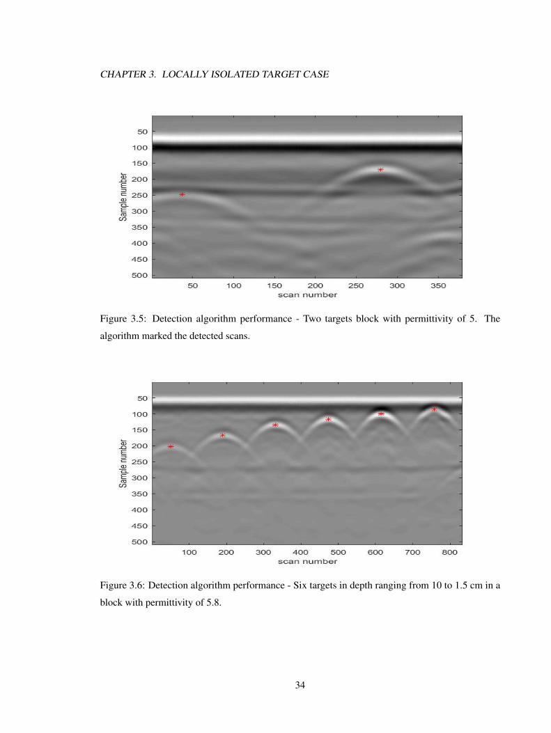
Figure 3.7: Detection algorithm performance - Six targets in depth ranging from 10 to 1.5 cm in a
block with permittivity of 9.
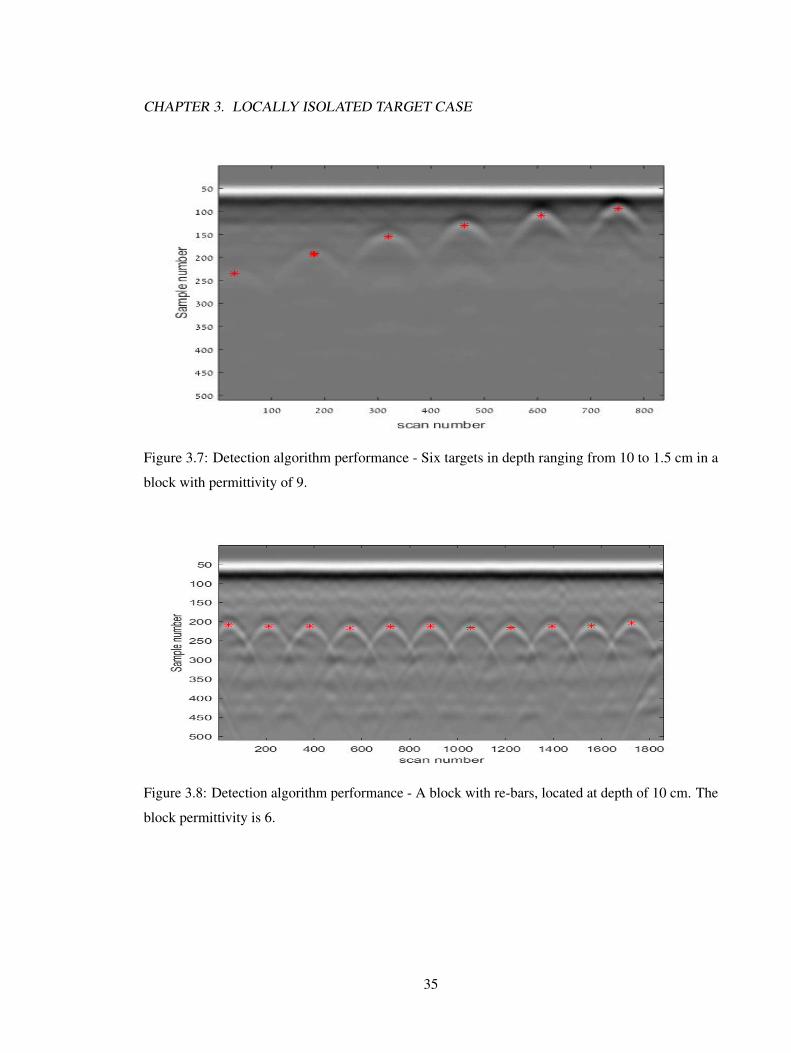
Figure 3.8: Detection algorithm performance - A block with re-bars, located at depth of 10 cm. The
block permittivity is 6.
35

CHAPTER 3. LOCALLY ISOLATED TARGET CASE
3.4 Discussion
The core ideas which drives the detection algorithm presented in this work were presented
in this chapter. They were developed into a full, working algorithm in itself, which is extremely
efficient and shows good performance metrics. Several parameters control this algorithm. The
most important one is the regression length - how many data points (scans) are used to perform the
regression analysis. This parameter presents some obvious trade-offs. On the one hand, the larger
the length is, the more noise reduction will be performed and the better the parameter estimation
will be. On the other hand, increasing this length means that the algorithm might miss targets from
the edge of the survey. Moreover, if the length is too large, the algorithm might miss all the targets
altogether when one target will start to cross another. For this work, this parameter was chosen
manually, though future work might consider adapting it in an iterative process to find an optimal
value. As will be shown in the next chapter, if multiple targets exists in the medium, in a close
proximity to one another, their hyperbole might cross, which will distort the shape of the curve in the
buffer. This in turn will lead to the wrong model parameter to be extracted, and the targets might be
missed altogether. This situation could easily be avoided if the buffer length is small enough.
The biggest shortcoming of the algorithm is in its focus on the (second) strongest reflection
in the signal as the one which contains the time information from the target. In case of multiple
layers and\or targets, this will not necessarily be the case. Mitigation to this will be the subject of
the next chapter.
36
Chapter 4
Generalization of the Automated Target
Detection Algorithm
The algorithm described in the previous chapter works very well as long as the assumptions
on which it was based hold. These are detailed in Section 2.1.2. The two weak assumption listed
there are the lack of interference that one target might introduce to another, and the fact that the
medium is locally homogeneous. The results of removing these two assumptions are the subject
of In this chapter. The effects created to the signal (and hence - to the buffer) by removing those
assumptions are explained in Section 4.1. Since these effects change the data stream at such an
early stage of the algorithm, significant modification was required to in order to enable the data
handling. While retaining the core ideas which guide the creation of the detection original algorithm,
the pre-processing stage underwent significant revision. This revision was done in order to be able to
detect the targets in any location they might be in the image - including under layers or other targets.
Additional sub-stage was added to the pre-processing stage of the original algorithm. In it, a target
trajectory is being assembled from the data stored in the buffer. It turned out that the pre-processing
stage was “too strong” - and many areas in the image were detected as targets (i.e. - increasing false
detection rate). For that reason, the decision stage was revised to incorporate more knowledge about
the targets. The end result of all of these modifications shall be described in Section 4.2, were the
algorithm will be re-built to accommodate for a more complex (and more realistic) scenario. The
results of the algorithm are presented in Section 4.4.
37
CHAPTER 4. GENERALIZATION OF THE AUTOMATED TARGET DETECTION ALGORITHM
4.1 Analyzing the Weakness of the Detection Algorithm
In a fully homogeneous medium, the only reflection which might arrive at the receiver
are those which result from the signal going from one layer to another. The boundary between the
two layers - where there is a theoretical discontinuity in the permittivity of the medium - will be the
point of refraction for the electromagnetic energy of the signal. In Section 2.1.2 this assumption (of a
locally homogeneous medium) was made, and the pre-processing stage was designed accordingly.
Step 2 of the algorithm was performed twice for each scan, on the two maximal peaks. The underlying
thought behind this was that these peaks were originated from the signal traveling via the direct path
(forming the strongest amplitude of the A-Scan) and the signal reflected off the target, forming the
second highest amplitudes in the signal. Since it was also assumed that the medium’ surface is flat
compared to the wavelength, one expect to detect the maximal amplitude of the signal at (roughly)
the same sample number at each A-scan. The design constraints included the overall efficiency
and minimal run time of the algorithm. For this reason the fact of the signal arriving at an almost
constant sample was fully exploited in the implementation. Detecting the second highest amplitude
called for a different approach, since no prior knowledge could be utilized in order to speed up the
search. To detect it efficiently, the fact that the maximal amplitude arrives at an (almost) constant
sample in the A-scans was used again: by removing the averaged scan (background) the algorithm
practically eliminated this part. Signals which were reflected off targets will exists only on few scans
out of the entire image, and the effect of such a removal on them will be minimal. This enable the
use for a simple search for a maximal amplitude on the background-removed scan, and eliminated
the need to detect all the maxima points of the scan, order them and choosing the strongest among
them. It should be noted that the permittivity of a “real-life” medium is never spatially constant, and
so reflection are generated at each and every time sample. However, the local change within the
mediums’ permittivity is typically small, and the amplitude of a reflection is relative to this change,
yielding that the reflection from the medium itself are usually weaker than the one coming from a
target, and the reflection from the target remains the (second) strongest signal in the A-scan. This
ceased to be the case if the medium is composed of multiple layers, as explained in Section 4.1.1.
Another assumption which was made in Section 2.1.2 was that of a locally isolated target.
when the medium contains multiple targets who are too close to one another, the resulted B-scan is
the composition of the reflection from all targets. This makes the separation of them challenging.
This subject is detailed in Section 4.1.2.
38
CHAPTER 4. GENERALIZATION OF THE AUTOMATED TARGET DETECTION ALGORITHM
4.1.1 Multi Layered Medium
If the assumption of a locally homogeneous medium does not hold (i.e. there is more than
a single horizontal layer in the scanned area), one might get a “hall-of-mirrors” effect: the signal will
bounce between the boundaries of the two layers, and the reflections will arrive at the receiver not
only from the surface of the medium and from the target, but also from multiples of the travel path.
The shape of the transmitted signal is Ricker Wavelet [35]. Combining this with the hall of mirrors
effect results in a “wavy” signal, where the multiple wavelets are visible in the A-Scan. In addition,
when the signal travels from a layer of relatively low permittivity to a layer with a higher one - the
polarity of the wavelet reverses. The received signal in this case will be composed of positive and
negative reflections, which might interfere with one another.
Multiple horizontal layers are very common in practice. Examples could be found in walls
(where the time range of the signal might be longer than the propagation time in the wall, causing
the signal to bounce inside the wall), as well as in paved roads (where there is the gravel underneath
the asphalt layer, and usually another bedrock underneath the gravel). Indeed, there are very few
cases where the assumption of a completely homogeneous medium does hold. There are cases,
however, where reflections from layer boundaries occlude the reflections from the target, so the
simple pre-processing approach of finding the target in a scan - by removing the background and
searching for the maximal peak - will not necessarily work in this case. An example for this is
presented in Figure 4.1, were a three layered medium was scanned. Note the bottom layer, which
might be an artifact due two energy bouncing from one layer to the next. The maximal sample in the
background removed signal in this case will be the reflection from the boundary between the first
and second layers and not from the target, leading to a complete miss-detection of the targets in the
second layer.
39
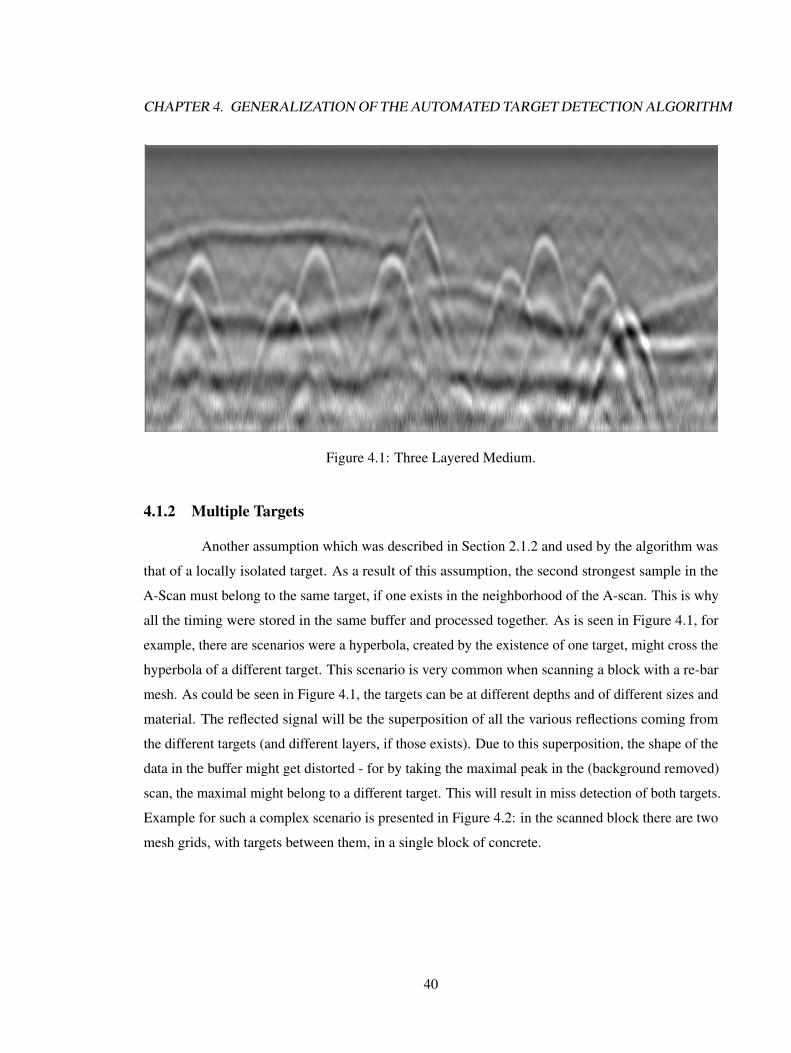
CHAPTER 4. GENERALIZATION OF THE AUTOMATED TARGET DETECTION ALGORITHM
Figure 4.1: Three Layered Medium.
4.1.2 Multiple Targets
Another assumption which was described in Section 2.1.2 and used by the algorithm was
that of a locally isolated target. As a result of this assumption, the second strongest sample in the
A-Scan must belong to the same target, if one exists in the neighborhood of the A-scan. This is why
all the timing were stored in the same buffer and processed together. As is seen in Figure 4.1, for
example, there are scenarios were a hyperbola, created by the existence of one target, might cross the
hyperbola of a different target. This scenario is very common when scanning a block with a re-bar
mesh. As could be seen in Figure 4.1, the targets can be at different depths and of different sizes and
material. The reflected signal will be the superposition of all the various reflections coming from
the different targets (and different layers, if those exists). Due to this superposition, the shape of the
data in the buffer might get distorted - for by taking the maximal peak in the (background removed)
scan, the maximal might belong to a different target. This will result in miss detection of both targets.
Example for such a complex scenario is presented in Figure 4.2: in the scanned block there are two
mesh grids, with targets between them, in a single block of concrete.
40
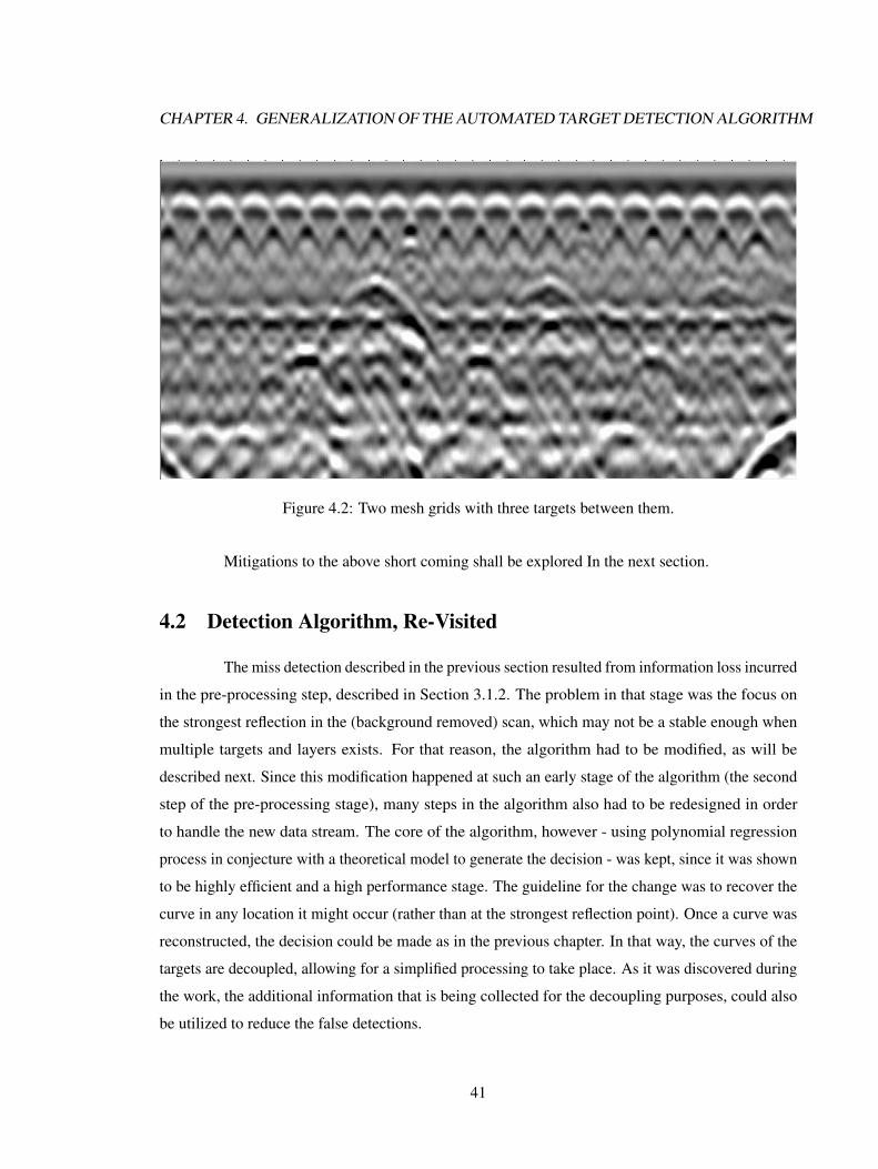
CHAPTER 4. GENERALIZATION OF THE AUTOMATED TARGET DETECTION ALGORITHM
Figure 4.2: Two mesh grids with three targets between them.
Mitigations to the above short coming shall be explored In the next section.
4.2 Detection Algorithm, Re-Visited
The miss detection described in the previous section resulted from information loss incurred
in the pre-processing step, described in Section 3.1.2. The problem in that stage was the focus on
the strongest reflection in the (background removed) scan, which may not be a stable enough when
multiple targets and layers exists. For that reason, the algorithm had to be modified, as will be
described next. Since this modification happened at such an early stage of the algorithm (the second
step of the pre-processing stage), many steps in the algorithm also had to be redesigned in order
to handle the new data stream. The core of the algorithm, however - using polynomial regression
process in conjecture with a theoretical model to generate the decision - was kept, since it was shown
to be highly efficient and a high performance stage. The guideline for the change was to recover the
curve in any location it might occur (rather than at the strongest reflection point). Once a curve was
reconstructed, the decision could be made as in the previous chapter. In that way, the curves of the
targets are decoupled, allowing for a simplified processing to take place. As it was discovered during
the work, the additional information that is being collected for the decoupling purposes, could also
be utilized to reduce the false detections.
41
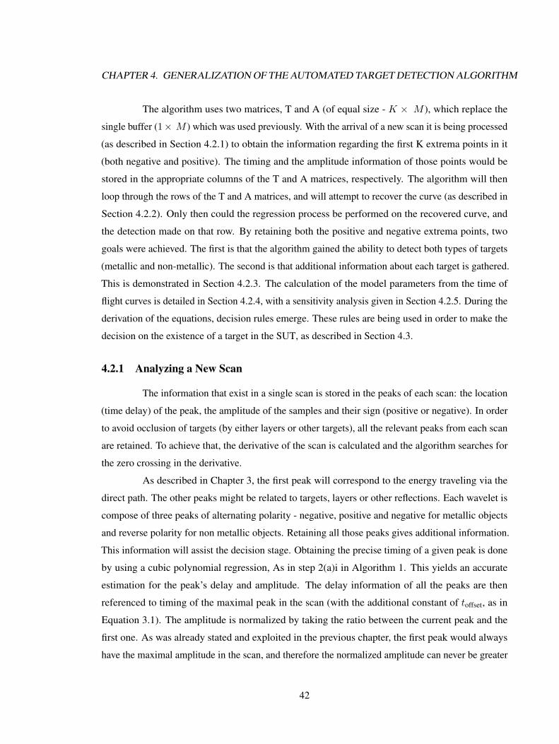
CHAPTER 4. GENERALIZATION OF THE AUTOMATED TARGET DETECTION ALGORITHM
The algorithm uses two matrices, T and A (of equal size - K × M ), which replace the
single buffer (1× M ) which was used previously. With the arrival of a new scan it is being processed
(as described in Section 4.2.1) to obtain the information regarding the first K extrema points in it
(both negative and positive). The timing and the amplitude information of those points would be
stored in the appropriate columns of the T and A matrices, respectively. The algorithm will then
loop through the rows of the T and A matrices, and will attempt to recover the curve (as described in
Section 4.2.2). Only then could the regression process be performed on the recovered curve, and
the detection made on that row. By retaining both the positive and negative extrema points, two
goals were achieved. The first is that the algorithm gained the ability to detect both types of targets
(metallic and non-metallic). The second is that additional information about each target is gathered.
This is demonstrated in Section 4.2.3. The calculation of the model parameters from the time of
flight curves is detailed in Section 4.2.4, with a sensitivity analysis given in Section 4.2.5. During the
derivation of the equations, decision rules emerge. These rules are being used in order to make the
decision on the existence of a target in the SUT, as described in Section 4.3.
4.2.1 Analyzing a New Scan
The information that exist in a single scan is stored in the peaks of each scan: the location
(time delay) of the peak, the amplitude of the samples and their sign (positive or negative). In order
to avoid occlusion of targets (by either layers or other targets), all the relevant peaks from each scan
are retained. To achieve that, the derivative of the scan is calculated and the algorithm searches for
the zero crossing in the derivative.
As described in Chapter 3, the first peak will correspond to the energy traveling via the
direct path. The other peaks might be related to targets, layers or other reflections. Each wavelet is
compose of three peaks of alternating polarity - negative, positive and negative for metallic objects
and reverse polarity for non metallic objects. Retaining all those peaks gives additional information.
This information will assist the decision stage. Obtaining the precise timing of a given peak is done
by using a cubic polynomial regression, As in step 2(a)i in Algorithm 1. This yields an accurate
estimation for the peak’s delay and amplitude. The delay information of all the peaks are then
referenced to timing of the maximal peak in the scan (with the additional constant of toffset, as in
Equation 3.1). The amplitude is normalized by taking the ratio between the current peak and the
first one. As was already stated and exploited in the previous chapter, the first peak would always
have the maximal amplitude in the scan, and therefore the normalized amplitude can never be greater
42

CHAPTER 4. GENERALIZATION OF THE AUTOMATED TARGET DETECTION ALGORITHM
than one (in absolute value). The normalization helps to eliminate differences in the signal amplitude
which might be the result of hardware changes (either from one system to another, or possibly due
to minute changes due to varied environmental conditions). They also mitigate differences in the
amplitude of the signal due to different permittivity values of different blocks. Once the peaks of
the scan were discovered and analyzed, they are being stored in the two matrices T and A (one for
the timing information and another for the amplitude, respectively). These matrices will generalize
the buffer used in Section 3.1.2, but they serve a similar purpose. This process is summarized in
Algorithm 2.
Algorithm 2 Scan Processing Procedure.Initialize the point counter by k ← 0.
For every sample n ∈ new scan
• Check the derivative of s in n. If the derivative changed its sign:
1. k ← k + 1.
2. Use polynomial regression to fit the N samples in the neighborhood of sample n.
3. On the first point (k = 0) set the reference time td and reference amplitude ad.
4. On any other point (K > 0) set the arrival time of the signal ta(k) and the amplitude
a(k).
5. The (relative) time of flight for that scan is given by
tflight(k) = ta(k)− td + toffset (4.1)
Where toffset is a constant of the system.
6. The normalized amplitude of the signal is given by
a(k) = a(k)/ad (4.2)
7. Store the tflight(k) and the a(k) values at the k-th row of the T and A matrices, respectively,
at the last column. If needed, discard the first values in that row and shift all other values
one place closer to the beginning of the matrices.
8. Verify that k ≤ K. If not - exit the loop.
43
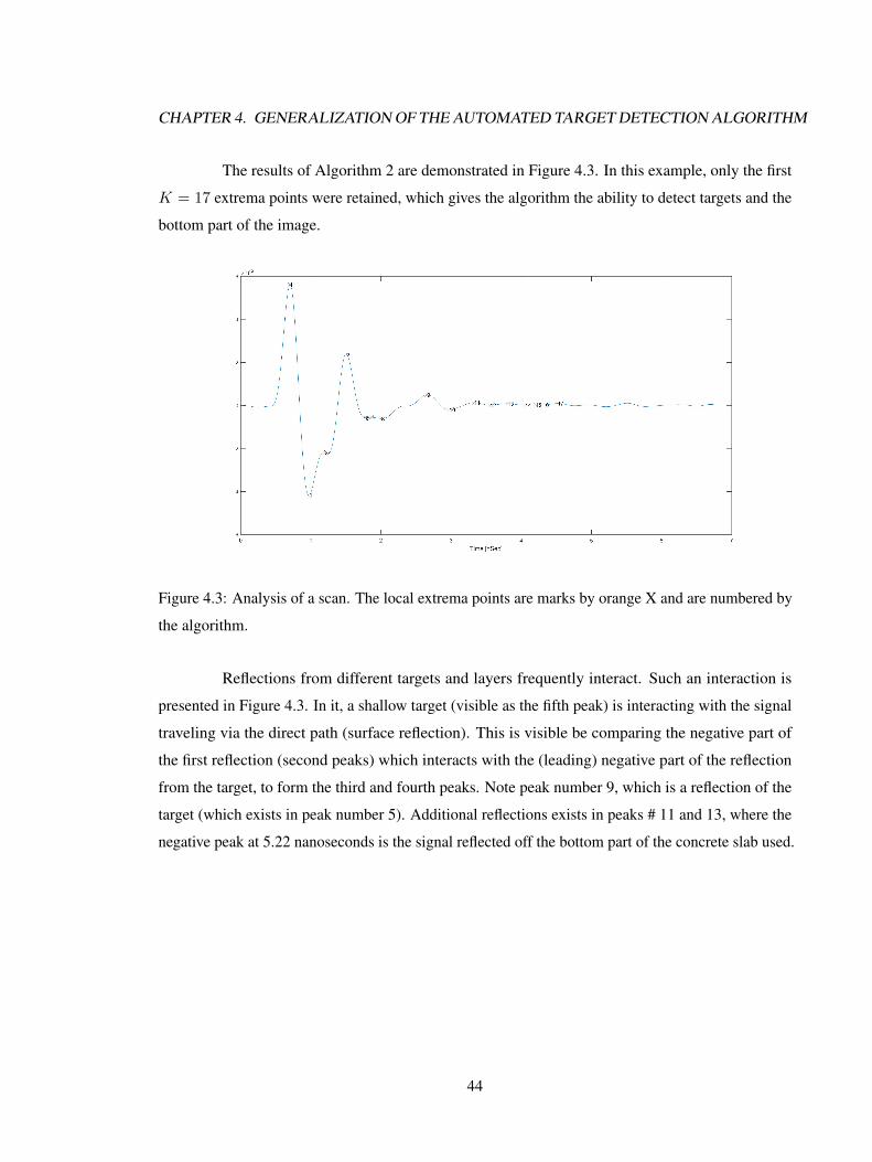
CHAPTER 4. GENERALIZATION OF THE AUTOMATED TARGET DETECTION ALGORITHM
The results of Algorithm 2 are demonstrated in Figure 4.3. In this example, only the first
K = 17 extrema points were retained, which gives the algorithm the ability to detect targets and the
bottom part of the image.
Figure 4.3: Analysis of a scan. The local extrema points are marks by orange X and are numbered by
the algorithm.
Reflections from different targets and layers frequently interact. Such an interaction is
presented in Figure 4.3. In it, a shallow target (visible as the fifth peak) is interacting with the signal
traveling via the direct path (surface reflection). This is visible be comparing the negative part of
the first reflection (second peaks) which interacts with the (leading) negative part of the reflection
from the target, to form the third and fourth peaks. Note peak number 9, which is a reflection of the
target (which exists in peak number 5). Additional reflections exists in peaks # 11 and 13, where the
negative peak at 5.22 nanoseconds is the signal reflected off the bottom part of the concrete slab used.
44
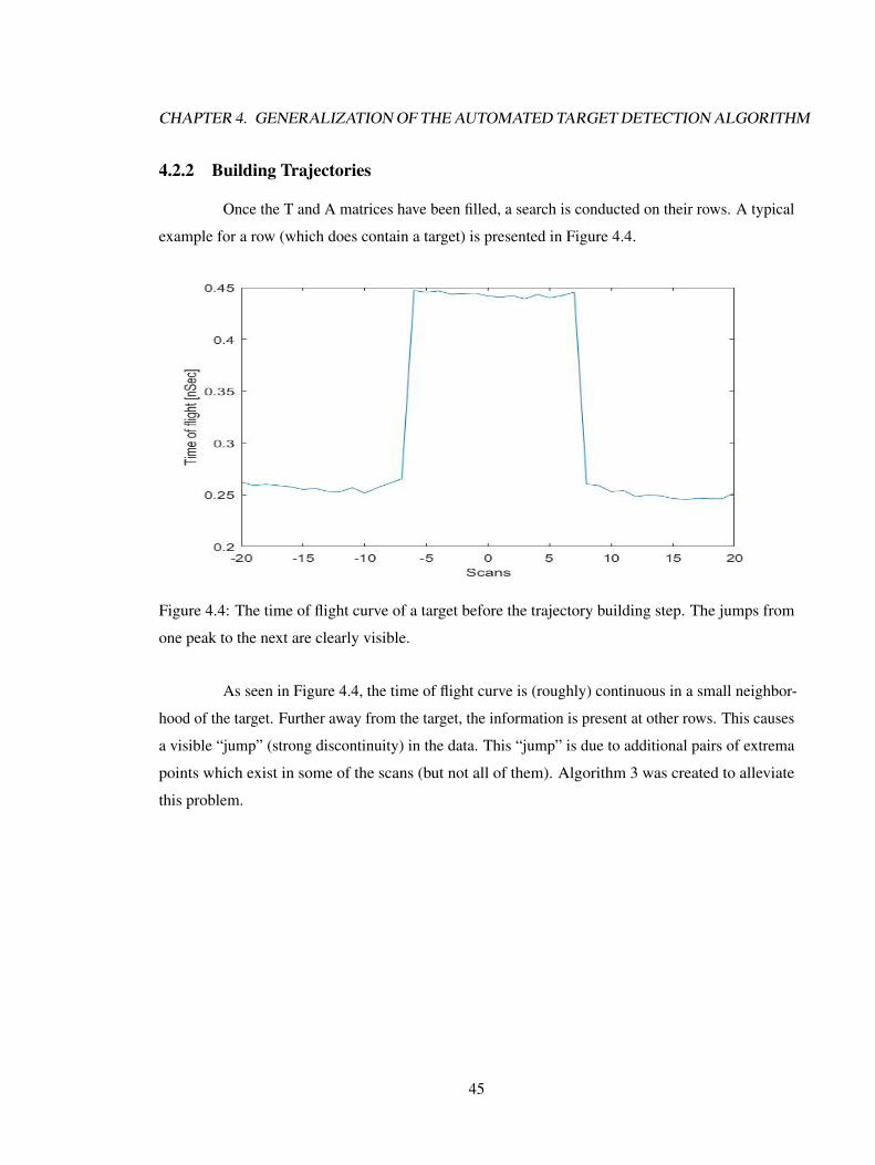
CHAPTER 4. GENERALIZATION OF THE AUTOMATED TARGET DETECTION ALGORITHM
4.2.2 Building Trajectories
Once the T and A matrices have been filled, a search is conducted on their rows. A typical
example for a row (which does contain a target) is presented in Figure 4.4.
Figure 4.4: The time of flight curve of a target before the trajectory building step. The jumps from
one peak to the next are clearly visible.
As seen in Figure 4.4, the time of flight curve is (roughly) continuous in a small neighbor-
hood of the target. Further away from the target, the information is present at other rows. This causes
a visible “jump” (strong discontinuity) in the data. This “jump” is due to additional pairs of extrema
points which exist in some of the scans (but not all of them). Algorithm 3 was created to alleviate
this problem.
45
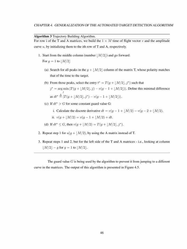
CHAPTER 4. GENERALIZATION OF THE AUTOMATED TARGET DETECTION ALGORITHM
Algorithm 3 Trajectory Building Algorithm.For row i of the T and A matrices, we build the 1 ×M time of flight vector v and the amplitude
curve u, by initializing them to the ith row of T and A, respectively.
1. Start from the middle column (number bM/2c) and go forward:
For g = 1 to bM/2c
(a) Search for all peaks in the g + bM/2c column of the matrix T, whose polarity matches
that of the time to the target.
(b) From those peaks, select the entry t∗ = T (g + bM/2c, j∗) such that
j∗ = arg minj|T (g + bM/2c, j)− v(g − 1 + bM/2c)|. Define this minimal difference
as dt∗ ∆= |T (g + bM/2c, j∗)− v(g − 1 + bM/2c)|.
(c) If dt∗ > G for some constant guard value G:
i. Calculate the discrete derivative dt = v(g − 1 + bM/2)− v(g − 2 + bM/2).
ii. v(g + bM/2) = v(g − 1 + bM/2) + dt.
(d) If dt∗ ≤ G, then v(g + bM/2) = T (g + bM/2c, j∗).
2. Repeat step 1 for u(g + bM/2), by using the A matrix instead of T.
3. Repeat steps 1 and 2, but for the left side of the T and A matrices - i.e., looking at column
bM/2c − g for g = 1 to bM/2c.
The guard value G is being used by the algorithm to prevent it from jumping to a different
curve in the matrices. The output of this algorithm is presented in Figure 4.5.
46
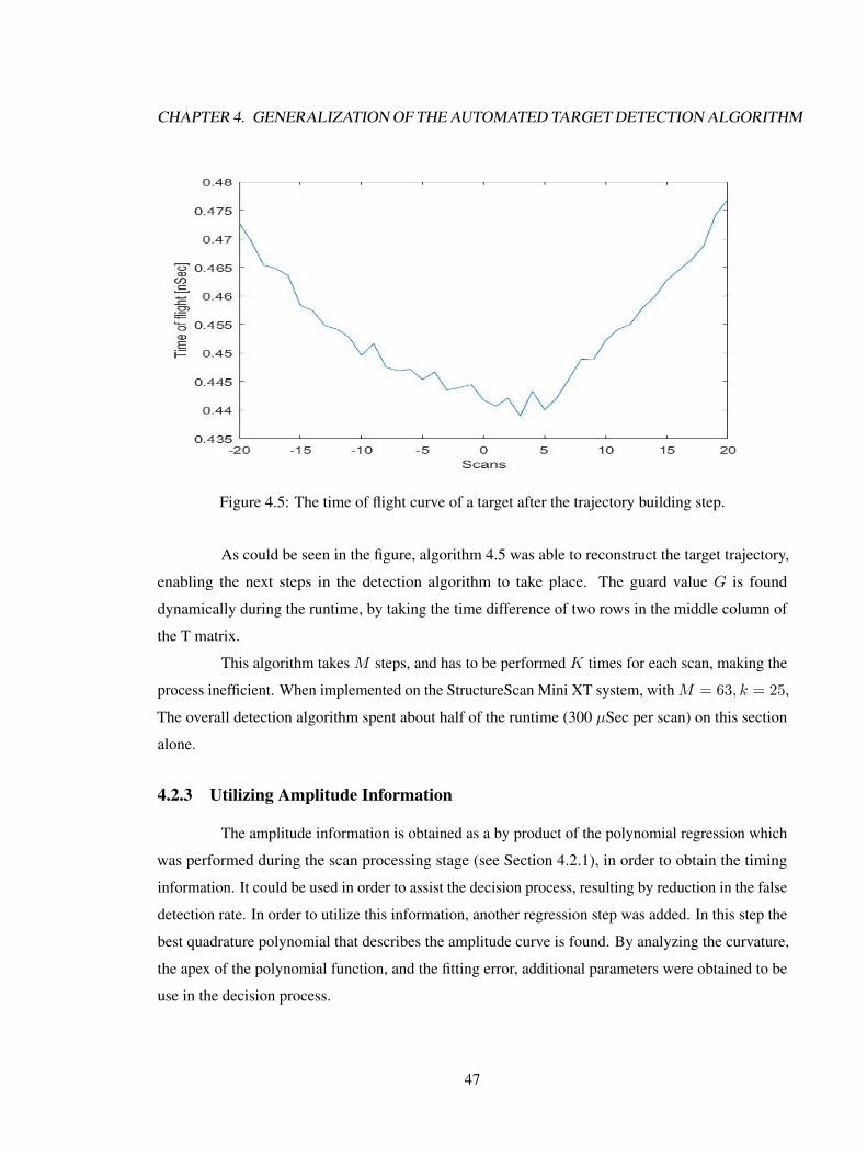
CHAPTER 4. GENERALIZATION OF THE AUTOMATED TARGET DETECTION ALGORITHM
Figure 4.5: The time of flight curve of a target after the trajectory building step.
As could be seen in the figure, algorithm 4.5 was able to reconstruct the target trajectory,
enabling the next steps in the detection algorithm to take place. The guard value G is found
dynamically during the runtime, by taking the time difference of two rows in the middle column of
the T matrix.
This algorithm takes M steps, and has to be performed K times for each scan, making the
process inefficient. When implemented on the StructureScan Mini XT system, with M = 63, k = 25,
The overall detection algorithm spent about half of the runtime (300 µSec per scan) on this section
alone.
4.2.3 Utilizing Amplitude Information
The amplitude information is obtained as a by product of the polynomial regression which
was performed during the scan processing stage (see Section 4.2.1), in order to obtain the timing
information. It could be used in order to assist the decision process, resulting by reduction in the false
detection rate. In order to utilize this information, another regression step was added. In this step the
best quadrature polynomial that describes the amplitude curve is found. By analyzing the curvature,
the apex of the polynomial function, and the fitting error, additional parameters were obtained to be
use in the decision process.
47
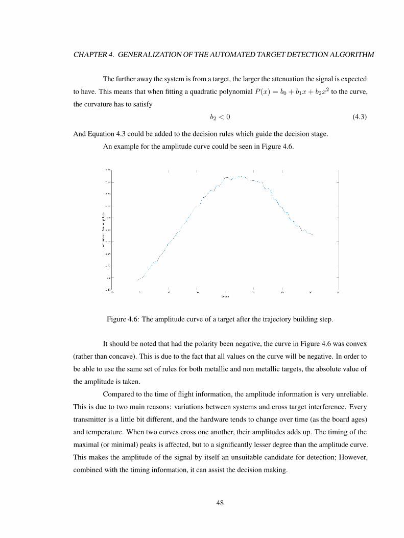
CHAPTER 4. GENERALIZATION OF THE AUTOMATED TARGET DETECTION ALGORITHM
The further away the system is from a target, the larger the attenuation the signal is expected
to have. This means that when fitting a quadratic polynomial P (x) = b0 + b1x+ b2x2 to the curve,
the curvature has to satisfy
b2 < 0 (4.3)
And Equation 4.3 could be added to the decision rules which guide the decision stage.
An example for the amplitude curve could be seen in Figure 4.6.
Figure 4.6: The amplitude curve of a target after the trajectory building step.
It should be noted that had the polarity been negative, the curve in Figure 4.6 was convex
(rather than concave). This is due to the fact that all values on the curve will be negative. In order to
be able to use the same set of rules for both metallic and non metallic targets, the absolute value of
the amplitude is taken.
Compared to the time of flight information, the amplitude information is very unreliable.
This is due to two main reasons: variations between systems and cross target interference. Every
transmitter is a little bit different, and the hardware tends to change over time (as the board ages)
and temperature. When two curves cross one another, their amplitudes adds up. The timing of the
maximal (or minimal) peaks is affected, but to a significantly lesser degree than the amplitude curve.
This makes the amplitude of the signal by itself an unsuitable candidate for detection; However,
combined with the timing information, it can assist the decision making.
48
CHAPTER 4. GENERALIZATION OF THE AUTOMATED TARGET DETECTION ALGORITHM
Other parameters which are used in the decision process are the model parameters - the
target depth h and the refraction coefficient of the block n. These are useful due to the fact the
they have physical meaning, and so their expected range could be pre-determined. Obtaining those
parameter from the time of flight curve is the subject of the next subsection.
4.2.4 Obtaining the Model Parameters
By equating a quadratic polynomial P (x) = a0 + a1x + a2x2 which describes a time
curve to the (second order) Taylor’s polynomial that describes the theoretical model, the model’s
parameter could be found (Equations 3.13 – 3.14). For completeness, the process of obtaining them
shall be repeated here. This allows to explain some of the decision rules used in the decision step.
Since the regression process is noise sensitive, a sensitivity analysis is performed in Section 4.2.5.
a2 =1
2t′′(0) =
n
c
h2
(h2 + ∆2)3/2(4.4)
a0 −a2
1
4a2= t(0) =
2n
c
√h2 + ∆2 (4.5)
Note that h ≥ 0, n ≥ 1, and define
Q∆=
√√√√a0 −a214a2
2a2=h2 + ∆2
h(4.6)
⇒ 0 = h2 −Qh+ ∆2 (4.7)
Note that a0, being the time of flight to the target, can never be negative. The curvature a2
likewise has to be strictly positive, since the time of flight has to increase the further the system is
from the target. For the SUT, one expect the center of the curve (x = − a12a2
) to be close enough to
the scan, which means that |a1| is sufficiently small, so that Q is well defined.
For the StructureScan Mini XT system, the desired target range is
0 < h ≤ 0.2[m] (4.8)
Equation 4.7 has two solutions:
h1,2 =Q
2±√Q2
4−∆2 (4.9)
49
CHAPTER 4. GENERALIZATION OF THE AUTOMATED TARGET DETECTION ALGORITHM
To ensure that the two solutions are real, Q has to satisfy
Q ≥ 2∆ (4.10)
Equations 4.8 and 4.10 could be added to the decision rules, along with the requirement
for a2 > 0 and a small enough center∣∣∣ a12a2
∣∣∣ < C for some constant C.
Using Equations 4.5 and 4.9, one gets a solution to the refraction coefficient n:
n1,2 =
(a0 −
a21
4a2
)c
2√h2
1,2 + ∆2= (4.11)
=
(a0 −
a21
4a2
)c
2√Qh1,2
Where the last equation holds because h1,2 are the solutions to Equation 4.7.
Equation 4.11 assists in determining the correct target depth h - for the value of both
parameters has to be within normal range. For the StructureScan Mini XT system, this range was set
to be
√5 ≤ n =
√εr ≤
√8 (4.12)
Note that for a large enough value of Q, the correct solution to Equations 4.9 – 4.11 will beh = 0.5Q−√
0.25Q2 −∆2
n = c2
(a0 −
a214a2
)(Qh)−1/2
(4.13)
Equation 4.13 is well defined, since Q ≥ 2∆ and h > 0.
4.2.5 Sensitivity Analysis of the Model Parameters
The regression process is sensitive to noise in the samples, so one naturally expects the
coefficients of the resulted polynomial {a0, a1, a2} to be slightly off from their nominal value. This
section explores the effect of “being slightly off”, to analyze how sensitive will the model parameters
are to the variations in the coefficient. Noting that the time of flight curve of a target should be
centralized to the scan, this analysis will begin by assuming that a1 ≈ 0, and so this coefficient has
little (if at all) effect on the model parameters. This section will therefore focus on analyzing the
effects of small perturbations in the curve’ offset a0 and curvature a2.
50
CHAPTER 4. GENERALIZATION OF THE AUTOMATED TARGET DETECTION ALGORITHM
1. Sensitivity to perturbation in the curvature. Let a2 = a2 + δa2, where δa2 << a2. From
Equation 4.6:
Q∆=
√a0
2a2 + 2δa2=
√a0
2a2
1√1 + δa2
a2
≈
≈√
a0
2a2
(1− δa2
2a2
)⇒ δQ = Q− Q =
Q
2a2δa2 (4.14)
2. Sensitivity to perturbation in the curve offset.
Q =
√a0 + δa0
2a2=
=
√a0
2a2
√1 +
δa0
a0≈
≈ Q(
1 +δa0
2a0
)(4.15)
⇒ δQ =Q
2a0δa0 (4.16)
Typical values for the offset are few nanosecond (1 < a0 < 12 for the StructureScan
MiniXT System) where typical values for the curvature range from 30 to 120 [nSec/m2], making Q
more sensitive to the offset than to the curvature. The typical range for Q is obtained by combining
the ranges mentioned above:
2∆ = 0.06 < Q < 2[m] (4.17)
51
CHAPTER 4. GENERALIZATION OF THE AUTOMATED TARGET DETECTION ALGORITHM
The sensitivity of the depth to a perturbation in Q would be:
h = 0.5(Q+ δQ)−√
0.25(Q+ δQ
)2−∆2 ≈ (4.18)
≈ 0.5(Q+ δQ)−√
0.25(Q2 + 2QδQ
)−∆2 =
= 0.5(Q+ δQ)−√
0.25Q2 −∆2
√1 +
0.5QδQ
0.25Q2 −∆2≈
≈ 0.5(Q+ δQ)−√
0.25Q2 −∆2
(1 +
0.25Q
0.25Q2 −∆2δQ
)=
= h+
0.5− 0.25Q√0.25Q2 −∆2
δQ =
= h+1
2
[1−
(1− 4∆2
Q2
)−1/2]δQ (4.19)
⇒ δh =1
2
[1−
(1− 4∆2
Q2
)−1/2]δQ (4.20)
By using the range for Q, one gets that δh ≈ 3δQ - so they are the same order of magnitude.
The sensitivity of the refraction coefficient would be:
n =c
2
(a0 −
a21
4a2+ δa
)[(Q+ δQ)(h+ δh)
]−1/2≈
≈ c
2
(a0 −
a21
4a2+ δa
)(Qh+ hδQ+ Qδh
)−1/2=
=c
2
(a0 −
a21
4a2+ δa
)(Qh+
[h+
Q
2
(1−
(1− 4∆2
Q2
)−1/2)]
δQ
)−1/2
=
=c
2
(a0 −
a21
4a2+ δa
)(Qh)−1/2
1 +
h+ Q2
[1−
(1− 4∆2
Q2
)−1/2]
QhδQ
−1/2
≈
≈ n
1−h+ Q
2
[1−
(1− 4∆2
Q2
)−1/2]
2QhδQ
+δa√Qh
(4.21)
⇒ δn =
h+ Q2
[1−
(1− 4∆2
Q2
)−1/2]
2QhnδQ+
δa√Qh
(4.22)
52
CHAPTER 4. GENERALIZATION OF THE AUTOMATED TARGET DETECTION ALGORITHM
Where δa is either δa0 in the case of perturbation in the offset or a218a2δa2 in case of a
perturbation in the curvature. Noting that a218a2
<< 1, this part could be neglected for the curvature.
Since both h and Q could be quite small, the refraction coefficient is significantly more sensitive to
any error which might be in the measurements. For that reason, when designing the final decision
boundaries, one needs to extend them beyond the physical limit of the material. This allows noisy
targets to be detected.
4.3 Decision Making Stage
During the previous steps of the algorithm, the GPR image was analyzed and converted
into potential targets. When a new scan arrives, the T and A matrices get updated. The pre-processing
stage continues by re-ordering the information in the rows of the T and A matrices, as was described
in Algorithm 3. The next step is to use quadratic polynomial regression on each (ordered) row, to
obtain the polynomial coefficient and the fitting error of the regression. From these coefficients, one
can extract the model parameters, as was described in Section 4.2.4. These steps converted the image
into potential targets, in a way that preserved the physical information of the signal, thus enabling
an efficient detection stage. Since every potential target would consist of three rows in the T and A
matrices, one gets that every potential target have 32 parameters which describe it:
• 18 polynomial coefficients and 6 fitting error values - the linf norm of the fitting error - from
the regression process of each of the six rows.
• Three estimations for the depth and dielectric, as predicted be Equation 4.13, from the time
curves.
• The polarity of the target (whether the middle row contains maxima or minima information).
• The sample number in which the target exists.
These 32 parameters define the parameter space, where each potential target is a single
point in this space. In order to ensure a high probability of detection while maintaining low false
detection rate, one needs the decision boundaries to tightly-fit the true target (i.e., minimizing the
volume in which the true targets exists). This could be achieved in different approaches. In this
work, the decision rules (which define the decision boundaries) were found manually: first, all the
GPR images were analyzed and manually annotated. In this stage, the decision rules were adjusted
to ensure that every true target will get detected. The targets were then added to a database. After
53
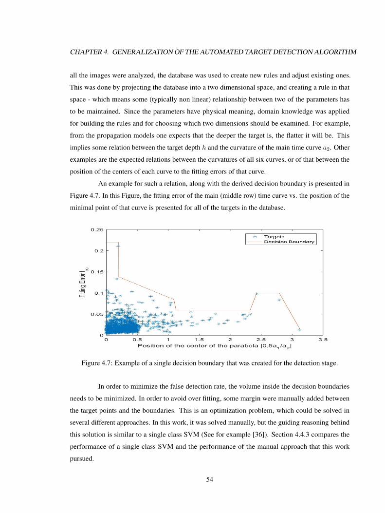
CHAPTER 4. GENERALIZATION OF THE AUTOMATED TARGET DETECTION ALGORITHM
all the images were analyzed, the database was used to create new rules and adjust existing ones.
This was done by projecting the database into a two dimensional space, and creating a rule in that
space - which means some (typically non linear) relationship between two of the parameters has
to be maintained. Since the parameters have physical meaning, domain knowledge was applied
for building the rules and for choosing which two dimensions should be examined. For example,
from the propagation models one expects that the deeper the target is, the flatter it will be. This
implies some relation between the target depth h and the curvature of the main time curve a2. Other
examples are the expected relations between the curvatures of all six curves, or of that between the
position of the centers of each curve to the fitting errors of that curve.
An example for such a relation, along with the derived decision boundary is presented in
Figure 4.7. In this Figure, the fitting error of the main (middle row) time curve vs. the position of the
minimal point of that curve is presented for all of the targets in the database.
Figure 4.7: Example of a single decision boundary that was created for the detection stage.
In order to minimize the false detection rate, the volume inside the decision boundaries
needs to be minimized. In order to avoid over fitting, some margin were manually added between
the target points and the boundaries. This is an optimization problem, which could be solved in
several different approaches. In this work, it was solved manually, but the guiding reasoning behind
this solution is similar to a single class SVM (See for example [36]). Section 4.4.3 compares the
performance of a single class SVM and the performance of the manual approach that this work
pursued.
54
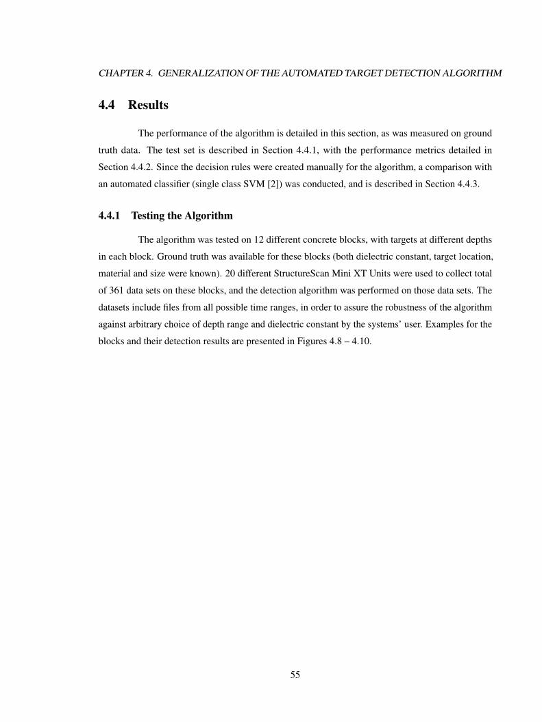
CHAPTER 4. GENERALIZATION OF THE AUTOMATED TARGET DETECTION ALGORITHM
4.4 Results
The performance of the algorithm is detailed in this section, as was measured on ground
truth data. The test set is described in Section 4.4.1, with the performance metrics detailed in
Section 4.4.2. Since the decision rules were created manually for the algorithm, a comparison with
an automated classifier (single class SVM [2]) was conducted, and is described in Section 4.4.3.
4.4.1 Testing the Algorithm
The algorithm was tested on 12 different concrete blocks, with targets at different depths
in each block. Ground truth was available for these blocks (both dielectric constant, target location,
material and size were known). 20 different StructureScan Mini XT Units were used to collect total
of 361 data sets on these blocks, and the detection algorithm was performed on those data sets. The
datasets include files from all possible time ranges, in order to assure the robustness of the algorithm
against arbitrary choice of depth range and dielectric constant by the systems’ user. Examples for the
blocks and their detection results are presented in Figures 4.8 – 4.10.
55
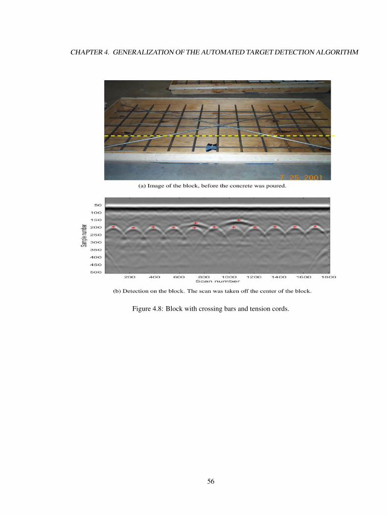
CHAPTER 4. GENERALIZATION OF THE AUTOMATED TARGET DETECTION ALGORITHM
Figure 4.8: Block with crossing bars and tension cords.
56
CHAPTER 4. GENERALIZATION OF THE AUTOMATED TARGET DETECTION ALGORITHM
Figure 4.9: Block with Pan Decking.
57
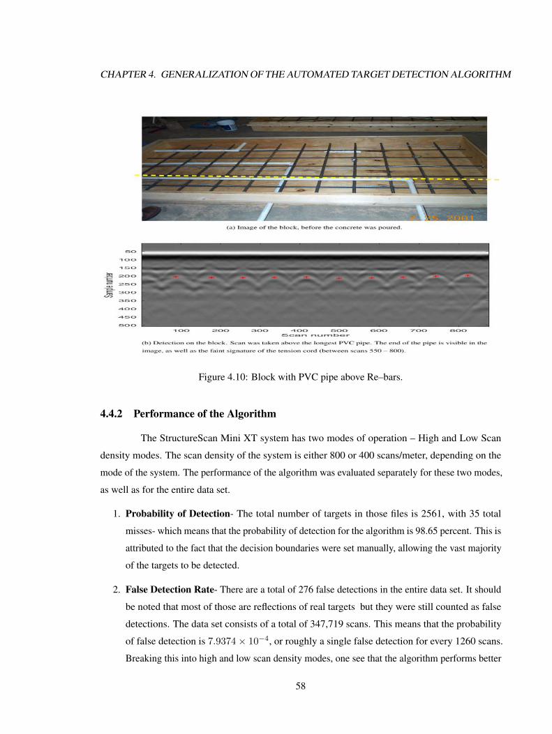
CHAPTER 4. GENERALIZATION OF THE AUTOMATED TARGET DETECTION ALGORITHM
Figure 4.10: Block with PVC pipe above Re–bars.
4.4.2 Performance of the Algorithm
The StructureScan Mini XT system has two modes of operation – High and Low Scan
density modes. The scan density of the system is either 800 or 400 scans/meter, depending on the
mode of the system. The performance of the algorithm was evaluated separately for these two modes,
as well as for the entire data set.
1. Probability of Detection- The total number of targets in those files is 2561, with 35 total
misses- which means that the probability of detection for the algorithm is 98.65 percent. This is
attributed to the fact that the decision boundaries were set manually, allowing the vast majority
of the targets to be detected.
2. False Detection Rate- There are a total of 276 false detections in the entire data set. It should
be noted that most of those are reflections of real targets but they were still counted as false
detections. The data set consists of a total of 347,719 scans. This means that the probability
of false detection is 7.9374× 10⁻⁴, or roughly a single false detection for every 1260 scans.
Breaking this into high and low scan density modes, one see that the algorithm performs better
58
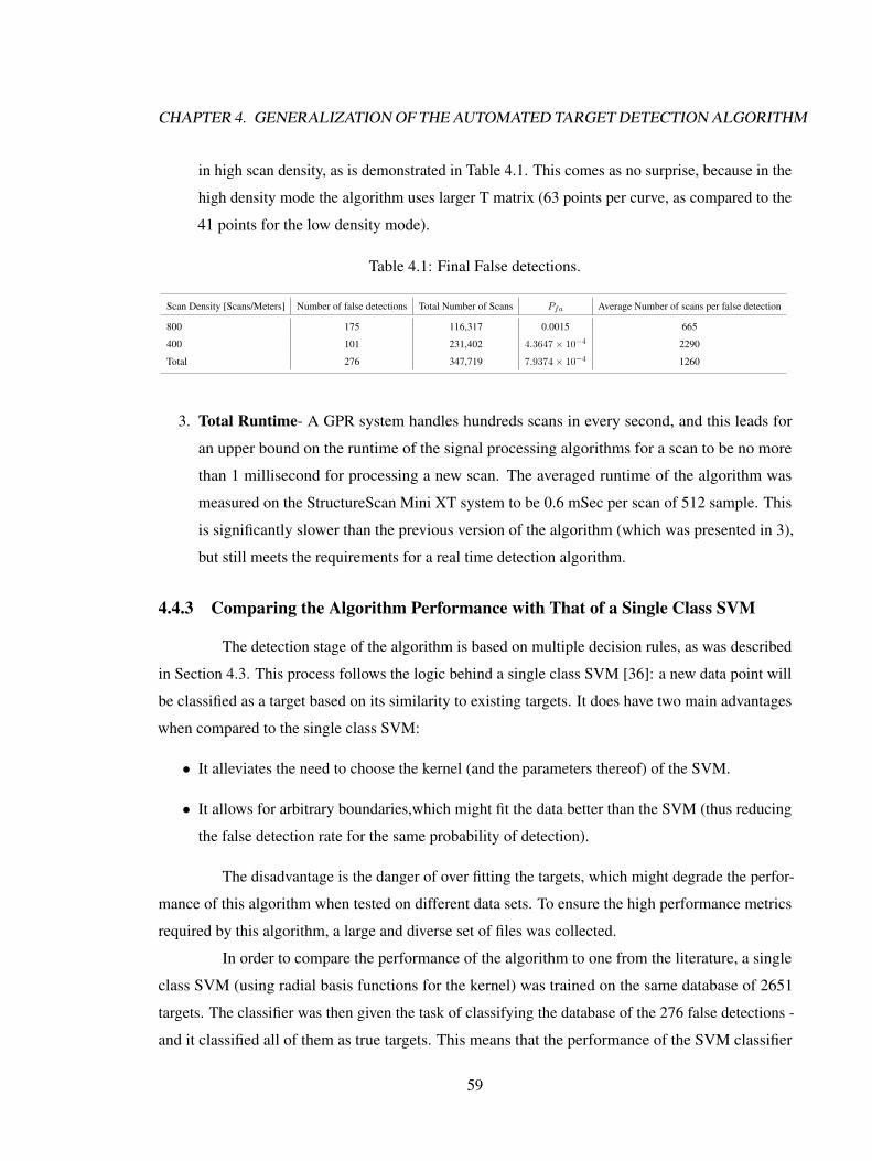
CHAPTER 4. GENERALIZATION OF THE AUTOMATED TARGET DETECTION ALGORITHM
in high scan density, as is demonstrated in Table 4.1. This comes as no surprise, because in the
high density mode the algorithm uses larger T matrix (63 points per curve, as compared to the
41 points for the low density mode).
Table 4.1: Final False detections.
Scan Density [Scans/Meters] Number of false detections Total Number of Scans Pfa Average Number of scans per false detection
800 175 116,317 0.0015 665
400 101 231,402 4.3647× 10⁻⁴ 2290
Total 276 347,719 7.9374× 10⁻⁴ 1260
3. Total Runtime- A GPR system handles hundreds scans in every second, and this leads for
an upper bound on the runtime of the signal processing algorithms for a scan to be no more
than 1 millisecond for processing a new scan. The averaged runtime of the algorithm was
measured on the StructureScan Mini XT system to be 0.6 mSec per scan of 512 sample. This
is significantly slower than the previous version of the algorithm (which was presented in 3),
but still meets the requirements for a real time detection algorithm.
4.4.3 Comparing the Algorithm Performance with That of a Single Class SVM
The detection stage of the algorithm is based on multiple decision rules, as was described
in Section 4.3. This process follows the logic behind a single class SVM [36]: a new data point will
be classified as a target based on its similarity to existing targets. It does have two main advantages
when compared to the single class SVM:
• It alleviates the need to choose the kernel (and the parameters thereof) of the SVM.
• It allows for arbitrary boundaries,which might fit the data better than the SVM (thus reducing
the false detection rate for the same probability of detection).
The disadvantage is the danger of over fitting the targets, which might degrade the perfor-
mance of this algorithm when tested on different data sets. To ensure the high performance metrics
required by this algorithm, a large and diverse set of files was collected.
In order to compare the performance of the algorithm to one from the literature, a single
class SVM (using radial basis functions for the kernel) was trained on the same database of 2651
targets. The classifier was then given the task of classifying the database of the 276 false detections -
and it classified all of them as true targets. This means that the performance of the SVM classifier
59
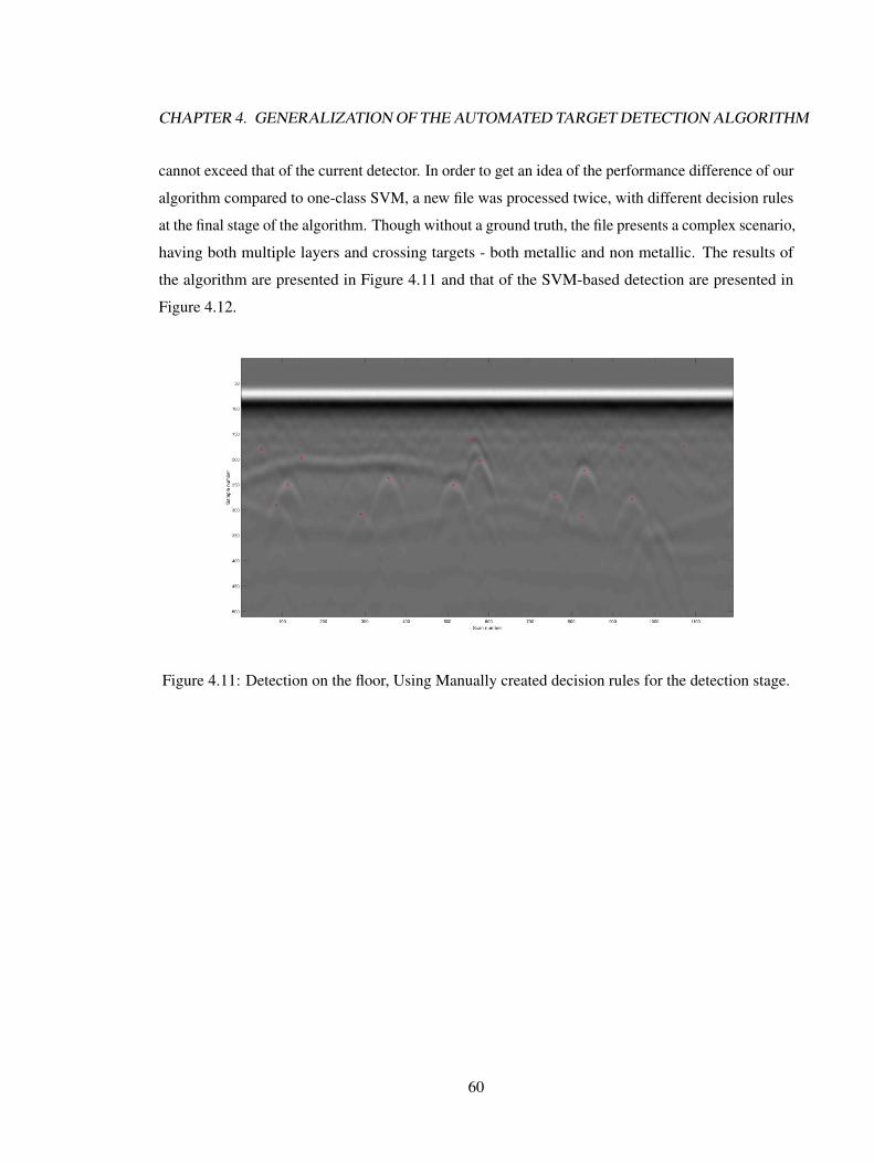
CHAPTER 4. GENERALIZATION OF THE AUTOMATED TARGET DETECTION ALGORITHM
cannot exceed that of the current detector. In order to get an idea of the performance difference of our
algorithm compared to one-class SVM, a new file was processed twice, with different decision rules
at the final stage of the algorithm. Though without a ground truth, the file presents a complex scenario,
having both multiple layers and crossing targets - both metallic and non metallic. The results of
the algorithm are presented in Figure 4.11 and that of the SVM-based detection are presented in
Figure 4.12.
Figure 4.11: Detection on the floor, Using Manually created decision rules for the detection stage.
60
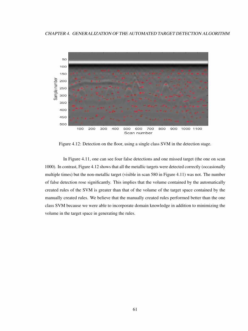
CHAPTER 4. GENERALIZATION OF THE AUTOMATED TARGET DETECTION ALGORITHM
Figure 4.12: Detection on the floor, using a single class SVM in the detection stage.
In Figure 4.11, one can see four false detections and one missed target (the one on scan
1000). In contrast, Figure 4.12 shows that all the metallic targets were detected correctly (occasionally
multiple times) but the non-metallic target (visible in scan 580 in Figure 4.11) was not. The number
of false detection rose significantly. This implies that the volume contained by the automatically
created rules of the SVM is greater than that of the volume of the target space contained by the
manually created rules. We believe that the manually created rules performed better than the one
class SVM because we were able to incorporate domain knowledge in addition to minimizing the
volume in the target space in generating the rules.
61

Chapter 5
Discussion and Future Research
The current algorithm is built in a modular way, where almost each and every component
could be replaced and\or improved. The modules shall be described in this chapter, along with a
detailed analysis of their strengths and weaknesses, accompanied by suggestions for improving them.
It should be noted that the chapter follows the data stream of the system, and not the order of the
importance of the modules or the improvements.
5.1 Processing a New Scan
1. As the new scan arrives from the RADAR board, it is being filtered first. This is done for display
purposes, but it helps the algorithm by enabling the next step, which uses information about
the derivative of the scan. Currently this is a Band Pass (BP) Infinite Impulse Response (IIR)
filter, with fixed frequencies which were found to yield good results on a large enough
data sets. Another (single pole, HP IIR) filter works horizontally - In order to remove the
background. The purpose of these filters are removing undesired features from the image
(noise, reverberations of the signal, and layers, to name a few) and increase the contrast (SNR)
of the targets. Both filters could be redesigned and re-implement in several ways:
• Combining them into a single, two dimensional filter (mask).
• Replacing them by adaptive filters.
62
CHAPTER 5. DISCUSSION AND FUTURE RESEARCH
2. Using the derivative of the scan to find the extrema points. This part could be improved in
several ways:
• Using knowledge for the location of the extrema points in the previous scans to set a
starting point for the search for a them in the new scan.
• Parallelize the search.
• For some situations, certain points matter more than others. Examples include the single
target case, which was discussed in Chapter 3. Other examples might include the search
for voids (were minima points would be proffered) vs. metallic points (were maxima
points would be. By limiting the type of targets, the number of relevant points from each
scan would be halved, and the overall performance of the algorithm be increased.
5.2 Processing the T and A Matrices
1. The first (and possible the most crucial) step of this stage is going over the buffer and apply the
Curve Building algorithm (Algorithm 3), as described in Chapter 4. This algorithm is the most
inefficient part of the entire detection algorithm, taking more than half(!) the run time of the
entire algorithm. Future research might go into early detection and elimination of undesired
parts of the signal (at the scan processing stage), so as to eliminate the need for this part.
2. Using quadratic polynomial regression fitting on the resulted curve. This part is the heart of
the detection algorithm, were the shape of the curve is revealed. As a sub-step, the shape is
compared to the theoretical model, to solve for the model parameters. It is by no means the
only method to do so. Few possible alternatives would be
• Bayesian approach: using the model ofp(x|d = 1, h, n) = t(x, h, n) + noise in presence of a target
p(x|d = 0, h, n) = noise without the presence of a target(5.1)
With d being an indicator for the existence of a target and proper statistics for the noise
models as well as priors to the model parameters. An optimal detector could be designed,
which will (possibly as a by-product) uncover the model parameters from the data.
Though possible, this would not be a simple task, since the noise in the samples (or even
the curves) that do not contain a target at the center of them might be heavily influenced
by the presence of a target, layer or a reverberation of the signal.
63
CHAPTER 5. DISCUSSION AND FUTURE RESEARCH
• Maximal Likelihood approach: similar to the Bayesian approach, assuming that the
samples of a curves are the result of a model with unknown parameters (with added
noise) may lead to the finding the optimal parameters which best describe the data.
Although more restricted than the Bayesian approach, it may be more practical since it
avoids the problems of estimating the prior for the model parameters.
5.3 Decision Making
The algorithm described in this work suffers from a (relatively) high false alarm rate. In
order to reduce it, one might use off the shelf algorithms like SVM or Neural Networks to separate
targets from non targets, based on the target parameters. Another related research would be a full
analysis of the algorithm, to produce the performance curve of the algorithm and show the trade-off
between the false detection rate and the probability of detection.
5.4 Additional topics for research
This work presented a detection algorithm, and the sections above described possible
research directions related to this specific algorithm. However, the field of target detection for
geophysical purposes has other research directions in it. Several of them will be covered in this
section.
• In a given dataset there is typically a low number of targets - which means that it could be
treated as a sparse dataset. Advances in the field of Compressed Sensing might enable a
different detection algorithm, which would take advantage of this sparsity.
• A different approach might be to attempt reconstructing the volume by placing targets in it -
using Probabilistic Graphical Models (PGMs) for example.
• This work focused solely on 2D data. A different problem exists when combining multiple
datagrams into a 3D volume cube: there is the question of alignment, similar to the one existing
in producing Synthetic Aperture Radar Images. Detecting targets in a volume would require a
different algorithm, and possibly different approach altogether, than the one presented here.
64

Chapter 6
Conclusion
The knowledge of a target’ location might lead GPR users to try to uncover it, and the
knowledge of a region free of targets might assist GPR users in selecting a suitable location for
drilling. In both these cases, a high probability of detection and a low false detection rate is required.
Since at this stage the algorithm is meant to assist in the detection, and not to replace the operator
altogether, a stronger effort was put into obtaining the former, probably at the expense of the latter. It
is the author’s hope and belief that future works will improve the results presented here. This will
allow for creation of detections devices simple enough for the general public usage.
This work presents a good starting point for that goal - an efficient, real time target detection
algorithm to be used on geophysical data sets. It was implemented and tested on a single GPR system
(GSSI’s StructureScanTM Mini XT system), but it is a general algorithm and could be applied to any
geophysical dataset - from both GPR and seismic devices - provided that the basic model assumption
(of a Bi Static system) holds true for that system. At the core of the algorithm lies a simple shape
detection. Its efficiency is being achieved by preprocessing the image, so that the the targets are
being searched only at specific regions.
A typical GPR dataset has tens of thousands of pixels in it. In order to handle the vast
amount of data, the algorithm performs the following:
• Limit the search window to be of no more than 63 scans. At 512 samples per scan for the
StructureScan Mini XT system, this gives us 32,256 pixels.
• By selecting the appropriate pixels from each scan, only 20 pixels out of every 512 are retained
(reducing the data by a factor of 25).
65
CHAPTER 6. CONCLUSION
• By iterating through the resulting layers, only three out of the 20 are being processed (reducing
the data by a factor of 7).
• By processing together groups of 63 scans and fitting a parabola to the data points, 63 values
are reduced to just 3 (reducing the data again by a factor of 20).
The resulting is a target space with 32 parameters, and it was found to be sufficient to
provide us with a good separation between real targets and false detections. The decision boundaries
were found empirically, by analyzing datasets containing targets and ensuring that those targets are
inside the detection zone (i.e. - designing the detection zone boundaries so that real targets will be
detected). Compared to automated boundary setting algorithms, such as SVM or Neural Networks,
the fact that this was a manual process has two main advantages:
• It provides an easy was to ensure a high probability of detection, as was specified for the
algorithm. Indeed, the final algorithm reached a probability of detection exceeding 98%.
• It provides the freedom to create non linear boundaries, which might be more efficient to
compute and fit the targets more tightly than a linear combination of kernel functions. Indeed,
it bypass the problem of choosing the kernel functions altogether.
In creating this space, knowledge about how a GPR system operates was utilized. This
assisted the detection process by providing criteria for the detection process. In order to do so, several
common propagation models were investigated and compared. They were contrasted with real data,
providing guidance for future researchers to use the best model appropriate for their needs.
There are several novel items in this work; possibly the most important of them is the
relaxation of the homogeneous layers’ assumption. In most of the prior work, it was always assumed
that the ground is composed of (possibly several) homogeneous layers - which means that the ground
properties are constant within the layer. This work breaks the layer into (approximately vertical)
segments, and assumes that each layer is only homogeneous in each segment. Moreover, the segments
could overlap, which would mean that the requirement of a homogeneous medium could be relaxed
in a slightly different way - by allow the properties of the layer to vary slow enough, compared to
the segment size. The relaxed requirement would be that the change in the layer’s properties will
be small relative to their average value. Another novel idea was the use of a simple polynomial
regression to perform feature extraction and detect targets. Using this allows for a very efficient
algorithm - one that works in O(m) operations per scan, where m is the number of samples in each
scan. This, in addition to the other known properties of the regression analysis: reduces the overall
66
CHAPTER 6. CONCLUSION
noise in the output, and increases the robustness of the overall algorithm. The use of Polynomial
Regression combined with Taylor’s polynomial is unconventional. The reason that it works is that
the uncertainty of the regression procedure, induced by the noise in the samples, overlaps some of
the uncertainty region caused by the approximation error of the Taylor’s polynomial and the initial
error of the model itself.
An ancient claim is that “the better is the enemy of good”. Like many other things this
algorithm could be improved and enhanced. Several possible directions were already mentioned:
• Modify the pre-process stages. During the work on the algorithm, it was found to have a
crucial effect, and so modifying the pre-processing stage will change the overall performance
of the algorithm.
• Vary the algorithm parameters automatically, based on the data.
• Replace the “detection engine”- instead of using the regression process, one might use other
approaches in order to determine the model parameters. Two likely candidates for that would
be a Bayesian, and the Maximal Likelihood approached. The former approaches utilizes (or
learn) prior knowledge regarding the statistics of the data. The latter attempts to obtain the
optimal parameters which justify the data.
• Enhance the algorithm to detect other features in the datasets: layers, rectangular targets
(pan-decking, for example) and other feature that might be of interest.
And so this work by no means provides an absolute and final solution to the problem it set
out to resolve. It is the hope of the author that the reader will find this work provides a good enough
basis for further research, adaptation and tailoring to his\hers needs.
67
Appendix A
Calculating the Theoretical Curves
The different theoretical models which were presented in Chapter 2. In that Chapter, the
resulted (predicted) curves were contrasted with the measured curve of different targets in known
conditions. Though generating the curves for the Bi Static Model (see Section 2.1.5) and its derivative
is relatively simple, the set of Equations 2.2 – 2.10 needs some manipulations in order to easily
produce the curves. In this appendix these manipulations are presented. The curves for both the Full
Model (See Section 2.1.3) and the Elevated, Mono Static Model (see Section 2.1.4) are produced
using the same mechanism: Solving for the (one way) time of flight of the signal, when the transceiver
is at a known location (y,−g). For the Elevated, Mono Static Model, x = y, that is the transmitter
is at the exact point of the receiver. By doubling the resulted flight time, the two way flight time
is obtained. In order to calculate the two way time of flight for the Full model, for each location
x of the system, two (one way) flight times should be obtained: from the transmitter to the target
(y = x−∆) and from the target to the receiver (y = x+ ∆).
In order to calculate the one way flight time of the signal from an arbitrary point (y,−g)
to the target, which is located at (0, h)), denote the crossing point of the energy to/from the ground
by (p, 0) - see Figure A.1.
68
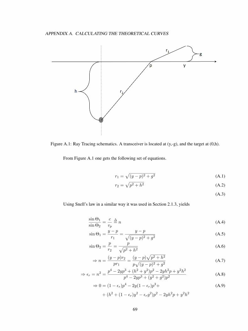
APPENDIX A. CALCULATING THE THEORETICAL CURVES
Figure A.1: Ray Tracing schematics. A transceiver is located at (y,-g), and the target at (0,h).
From Figure A.1 one gets the following set of equations.
r1 =√
(y − p)2 + g2 (A.1)
r2 =√p2 + h2 (A.2)
(A.3)
Using Snell’s law in a similar way it was used in Section 2.1.3, yields
sin Θ1
sin Θ2=
c
vp
∆= n (A.4)
sin Θ1 =y − pr1
=y − p√
(y − p)2 + g2(A.5)
sin Θ2 =p
r2=
p√p2 + h2
(A.6)
⇒ n =(y − p)r2
pr1=
(y − p)√p2 + h2
p√
(y − p)2 + g2(A.7)
⇒ εr = n2 =p4 − 2yp3 + (h2 + y2)p2 − 2yh2p+ y2h2
p4 − 2yp3 + (y2 + g2)p2(A.8)
⇒ 0 = (1− εr)p4 − 2y(1− εr)p3+ (A.9)
+ (h2 + (1− εr)y2 − εrg2)p2 − 2yh2p+ y2h2
69

APPENDIX A. CALCULATING THE THEORETICAL CURVES
Defining γ ∆= (εr − 1), one gets
0 = γp4 + 2γyp3− (A.10)
− (h2 + γy2 − εrg2)p2 + 2yh2p− y2h2
This is a polynomial equation of the fourth order, which could easily be resolved - for
example, via numerical methods. In general it will have four solutions. The correct solution has to
satisfy that p ∈ R
sgn(p) = sgn(y)
0 ≤ |p| ≤ |y|
(A.11)
Once the crossing point (p, 0) is found, the time of flight for the single sided problem is
given by
r1 =√
(y − p)2 + g2 (A.12)
r2 =√p2 + h2 (A.13)
t =r1 + nr2
c(A.14)
70

Appendix B
Sensitivity Analysis of the Propagation
Models
As a part of the of the detection algorithm, the model parameters are obtained, in order
to assist the decision making stage. For that reason, it would be beneficial if the theoretical model
used to predict the target’ shape was sensitive to the model parameters (target depth h and refraction
coefficient n), so that different curves would yield different parameters. As will be shown and
analyzed here, this is indeed the case for the model used (Polynomial Approximation to the Bi
Static Model – see Section 2.1.7). In practice, a target creates a unique shape; this means that the
information regarding the parameters should be available by studying its shape. However, due to
noise in and the limited precision of our measurements, obtaining those parameters might prove
difficult. Using the correct model is therefore crucial.
When examining the sensitivity of a model to its parameters, we shall define two criteria:
• The curve offset is defined as the two way propagation time to the target when the system is
directly above the target x = 0.
• The effect of the change in curve’ shape is defined as the change in the curve at x = 8 cm
from the target.
It should be noted that our choice of parameters is somewhat arbitrary, and other parameters
could have been used - for example, the l2 norm of the change in the curve. However, it was found
that these two are suffice for a qualitative analysis of the sensitivity of the model.
71
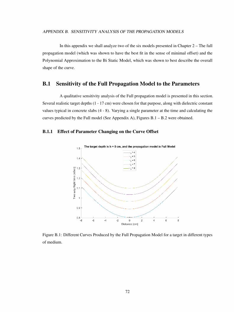
APPENDIX B. SENSITIVITY ANALYSIS OF THE PROPAGATION MODELS
In this appendix we shall analyze two of the six models presented in Chapter 2 – The full
propagation model (which was shown to have the best fit in the sense of minimal offset) and the
Polynomial Approximation to the Bi Static Model, which was shown to best describe the overall
shape of the curve.
B.1 Sensitivity of the Full Propagation Model to the Parameters
A qualitative sensitivity analysis of the Full propagation model is presented in this section.
Several realistic target depths (1 - 17 cm) were chosen for that purpose, along with dielectric constant
values typical in concrete slabs (4 - 8). Varying a single parameter at the time and calculating the
curves predicted by the Full model (See Appendix A), Figures B.1 – B.2 were obtained.
B.1.1 Effect of Parameter Changing on the Curve Offset
Figure B.1: Different Curves Produced by the Full Propagation Model for a target in different types
of medium.
72
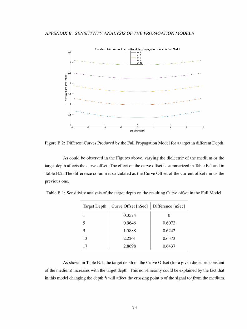
APPENDIX B. SENSITIVITY ANALYSIS OF THE PROPAGATION MODELS
Figure B.2: Different Curves Produced by the Full Propagation Model for a target in different Depth.
As could be observed in the Figures above, varying the dielectric of the medium or the
target depth affects the curve offset. The effect on the curve offset is summarized in Table B.1 and in
Table B.2. The difference column is calculated as the Curve Offset of the current offset minus the
previous one.
Table B.1: Sensitivity analysis of the target depth on the resulting Curve offset in the Full Model.
Target Depth Curve Offset [nSec] Difference [nSec]
1 0.3574 0
5 0.9646 0.6072
9 1.5888 0.6242
13 2.2261 0.6373
17 2.8698 0.6437
As shown in Table B.1, the target depth on the Curve Offset (for a given dielectric constant
of the medium) increases with the target depth. This non-linearity could be explained by the fact that
in this model changing the depth h will affect the crossing point p of the signal to\from the medium.
73

APPENDIX B. SENSITIVITY ANALYSIS OF THE PROPAGATION MODELS
Table B.2: Sensitivity analysis of the medium’s permittivity on the resulting Curve offset in the Full
Model.
Dielectric Constant εr Curve Offset [nSec] Curve Offset√εr
[nSec]
4 0.8039 0.4019
5 0.8886 0.3974
6 0.9646 0.3938
7 1.0340 0.3908
8 1.0982 0.3883
Changing the dielectric constant of the medium has a lesser effect on the Curve Offset than
the target depth - as one might expect. In addition, since the crossing point p is also affected by the
dielectric constant of the medium, one gets that the change in the ratio between the Curve Offset
and the refraction coefficient n =√εr is not constant. This, again, is explained by the fact that the
crossing point p moves towards the transceiver as we lower the dielectric.
74
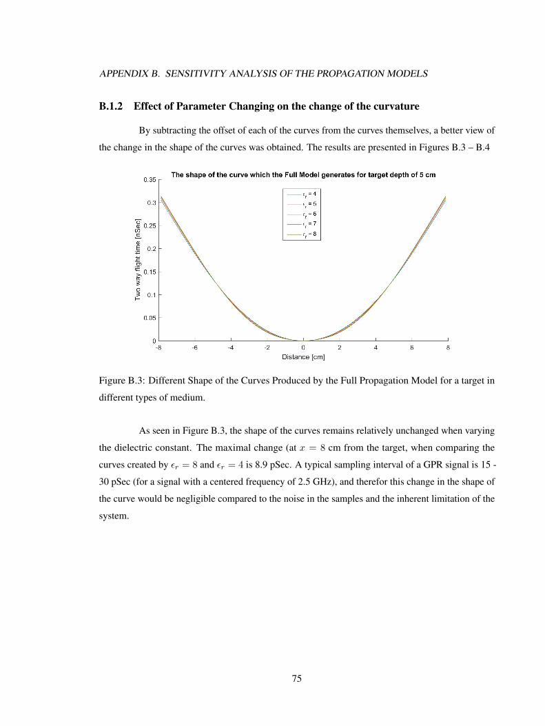
APPENDIX B. SENSITIVITY ANALYSIS OF THE PROPAGATION MODELS
B.1.2 Effect of Parameter Changing on the change of the curvature
By subtracting the offset of each of the curves from the curves themselves, a better view of
the change in the shape of the curves was obtained. The results are presented in Figures B.3 – B.4
Figure B.3: Different Shape of the Curves Produced by the Full Propagation Model for a target in
different types of medium.
As seen in Figure B.3, the shape of the curves remains relatively unchanged when varying
the dielectric constant. The maximal change (at x = 8 cm from the target, when comparing the
curves created by εr = 8 and εr = 4 is 8.9 pSec. A typical sampling interval of a GPR signal is 15 -
30 pSec (for a signal with a centered frequency of 2.5 GHz), and therefor this change in the shape of
the curve would be negligible compared to the noise in the samples and the inherent limitation of the
system.
75
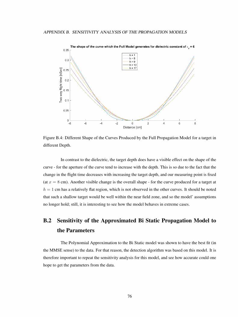
APPENDIX B. SENSITIVITY ANALYSIS OF THE PROPAGATION MODELS
Figure B.4: Different Shape of the Curves Produced by the Full Propagation Model for a target in
different Depth.
In contrast to the dielectric, the target depth does have a visible effect on the shape of the
curve - for the aperture of the curve tend to increase with the depth. This is so due to the fact that the
change in the flight time decreases with increasing the target depth, and our measuring point is fixed
(at x = 8 cm). Another visible change is the overall shape - for the curve produced for a target at
h = 1 cm has a relatively flat region, which is not observed in the other curves. It should be noted
that such a shallow target would be well within the near field zone, and so the model’ assumptions
no longer hold; still, it is interesting to see how the model behaves in extreme cases.
B.2 Sensitivity of the Approximated Bi Static Propagation Model to
the Parameters
The Polynomial Approximation to the Bi Static model was shown to have the best fit (in
the MMSE sense) to the data. For that reason, the detection algorithm was based on this model. It is
therefore important to repeat the sensitivity analysis for this model, and see how accurate could one
hope to get the parameters from the data.
76
APPENDIX B. SENSITIVITY ANALYSIS OF THE PROPAGATION MODELS
B.2.1 Analytical Analysis of the Sensitivity of the Model
The time of flight is given by Equation 2.24, which, along with Equations 2.25 – 2.27
enable a derivation of a full analytical sensitivity analysis.
t(n, h, x) ≈ 1
c
[t(0) +
1
2
∂t2
∂2x(0)x2
]= (B.1)
=2n√h2 + ∆2
c
[1 +
h2x2
2 (h2 + ∆2)2
]From Equation B.1 one gets a nice separation between the Curve Offset and it’s shape.
B.2.2 Effect of Parameter Changing on the Curve Offset
Using Equation B.1, we get the following response to a small perturbation δh in the Curve
Offset:
t(n, h+ δh, 0) =2n√
(h+ δh)2 + ∆2
c= (B.2)
=2n√h2 + ∆2 + 2hδh+ (δh)2
c≈
≈2n√h2 + ∆2
√1 + 2hδh
h2+∆2
c≈
≈ 2n√h2 + ∆2
c
(1 +
hδh
h2 + ∆2
)=
= t(n, h, 0) +2n
c
√1 +
(∆h
)2 δhAnd from Equation B.2 one can get an expression for the change in the Curve Offset
δt = t(n, h+ δh, 0)− t(n, h, 0) in response of a change δh to the target depth.
Similarly, given a small perturbation δn in the refraction coefficient, one gets
t(n+ δn, h, 0) =2(n+ δn)
√h2 + ∆2
c= (B.3)
= t(n+ δn, h, 0) +2√h2 + ∆2
cδn
Examples of the changes in The curve Offset are given in Figures B.5 - B.6 and in Tables
B.4 - B.4.
77
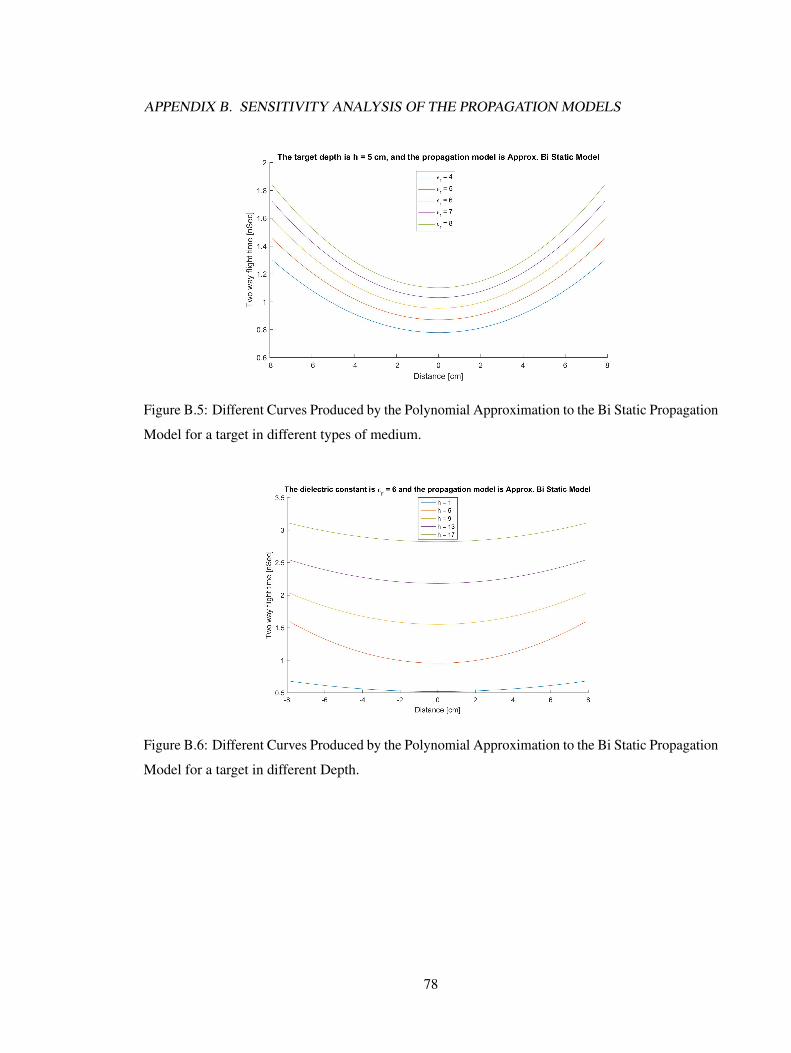
APPENDIX B. SENSITIVITY ANALYSIS OF THE PROPAGATION MODELS
Figure B.5: Different Curves Produced by the Polynomial Approximation to the Bi Static Propagation
Model for a target in different types of medium.
Figure B.6: Different Curves Produced by the Polynomial Approximation to the Bi Static Propagation
Model for a target in different Depth.
78
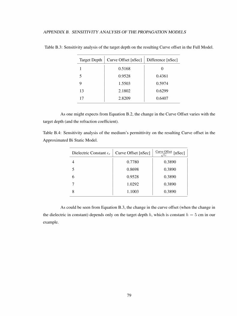
APPENDIX B. SENSITIVITY ANALYSIS OF THE PROPAGATION MODELS
Table B.3: Sensitivity analysis of the target depth on the resulting Curve offset in the Full Model.
Target Depth Curve Offset [nSec] Difference [nSec]
1 0.5168 0
5 0.9528 0.4361
9 1.5503 0.5974
13 2.1802 0.6299
17 2.8209 0.6407
As one might expects from Equation B.2, the change in the Curve Offset varies with the
target depth (and the refraction coefficient).
Table B.4: Sensitivity analysis of the medium’s permittivity on the resulting Curve offset in the
Approximated Bi Static Model.
Dielectric Constant εr Curve Offset [nSec] Curve Offset√εr
[nSec]
4 0.7780 0.3890
5 0.8698 0.3890
6 0.9528 0.3890
7 1.0292 0.3890
8 1.1003 0.3890
As could be seen from Equation B.3, the change in the curve offset (when the change in
the dielectric in constant) depends only on the target depth h, which is constant h = 5 cm in our
example.
79
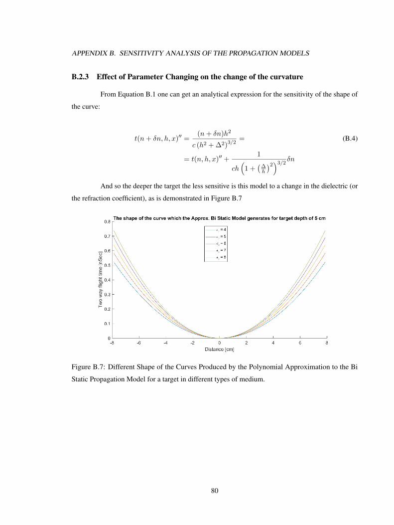
APPENDIX B. SENSITIVITY ANALYSIS OF THE PROPAGATION MODELS
B.2.3 Effect of Parameter Changing on the change of the curvature
From Equation B.1 one can get an analytical expression for the sensitivity of the shape of
the curve:
t(n+ δn, h, x)′′ =(n+ δn)h2
c (h2 + ∆2)3/2= (B.4)
= t(n, h, x)′′ +1
ch(
1 +(
∆h
)2)3/2δn
And so the deeper the target the less sensitive is this model to a change in the dielectric (or
the refraction coefficient), as is demonstrated in Figure B.7
Figure B.7: Different Shape of the Curves Produced by the Polynomial Approximation to the Bi
Static Propagation Model for a target in different types of medium.
80
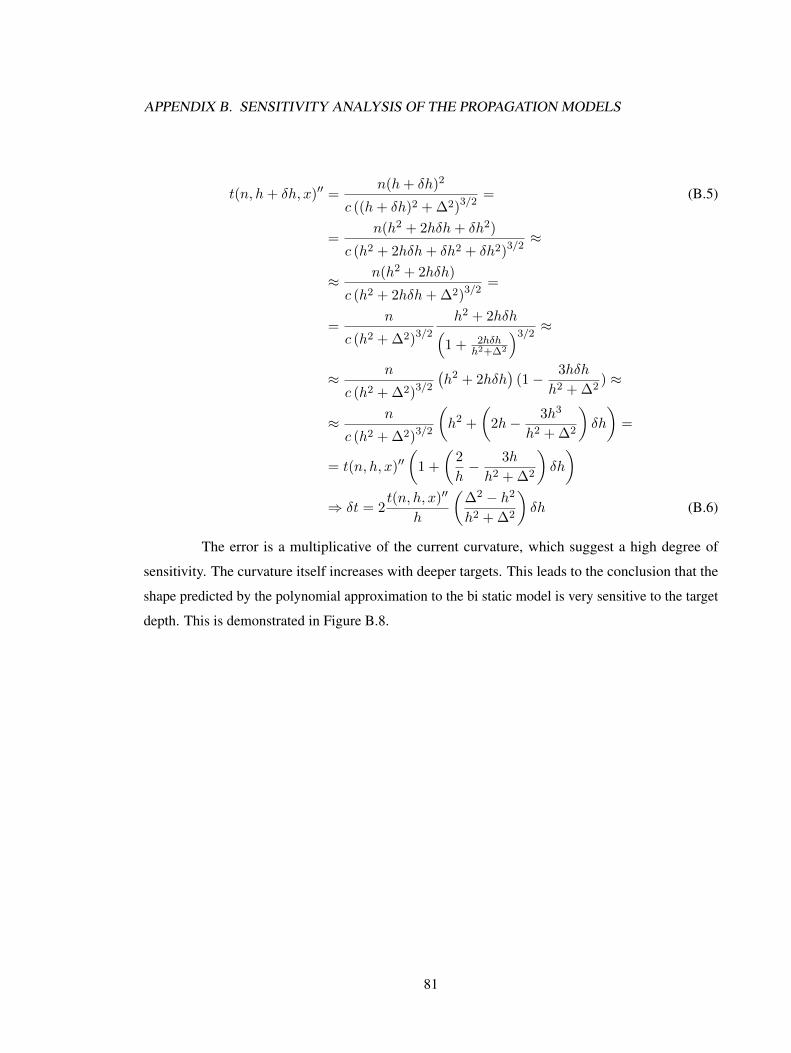
APPENDIX B. SENSITIVITY ANALYSIS OF THE PROPAGATION MODELS
t(n, h+ δh, x)′′ =n(h+ δh)2
c ((h+ δh)2 + ∆2)3/2= (B.5)
=n(h2 + 2hδh+ δh2)
c (h2 + 2hδh+ δh2 + δh2)3/2≈
≈ n(h2 + 2hδh)
c (h2 + 2hδh+ ∆2)3/2=
=n
c (h2 + ∆2)3/2
h2 + 2hδh(1 + 2hδh
h2+∆2
)3/2≈
≈ n
c (h2 + ∆2)3/2
(h2 + 2hδh
)(1− 3hδh
h2 + ∆2) ≈
≈ n
c (h2 + ∆2)3/2
(h2 +
(2h− 3h3
h2 + ∆2
)δh
)=
= t(n, h, x)′′(
1 +
(2
h− 3h
h2 + ∆2
)δh
)⇒ δt = 2
t(n, h, x)′′
h
(∆2 − h2
h2 + ∆2
)δh (B.6)
The error is a multiplicative of the current curvature, which suggest a high degree of
sensitivity. The curvature itself increases with deeper targets. This leads to the conclusion that the
shape predicted by the polynomial approximation to the bi static model is very sensitive to the target
depth. This is demonstrated in Figure B.8.
81
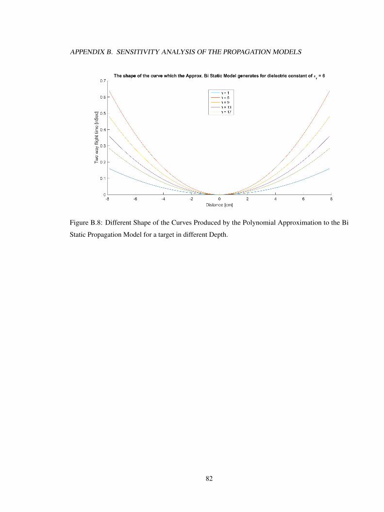
APPENDIX B. SENSITIVITY ANALYSIS OF THE PROPAGATION MODELS
Figure B.8: Different Shape of the Curves Produced by the Polynomial Approximation to the Bi
Static Propagation Model for a target in different Depth.
82
Bibliography
[1] F. C. Commission, “Fcc 02-48 - uwb regulations,” https://transition.fcc.gov/Bureaus/
Engineering Technology/Orders/2002/fcc02048.pdf.
[2] V. VAPNIK and C. CORTES, “Support-vector networks,” Machine Learning, no. 20, pp.
273–297, 1995.
[3] R. Yelf, “Where is true time zero?” in Tenth International Conference on Ground Penetrating
Radar, Delft, The Netherlands, 2004.
[4] S. Radzevicius, “Least-suare curve fitting for velocity and time zero,” in 2015 8th IWAGPR,
Florence, Italy, 2015.
[5] R. Sakaguchi, “Image processing methods applied to landmine detection in ground penetrating
radar,” Durham, NC, 2013.
[6] A. Manandhar, P. A. Torrione, L. M. Collins, and K. D. Morton, “Multiple-instance hidden
markov model for gpr-based landmine detection,” IEEE Transaction on Geoscience and Remote
Sensing, vol. 53, no. 4, pp. 1737–1745, 2015.
[7] U. S. Khan, W. Al-Nuaimy, and F. E. A. El-Samie, “Detection of landmines and underground
utilities from acoustic and gpr images with cepstral approach,” ELSEVIER Journal of Visual
Communication and Image Representation, vol. 21, no. 4, pp. 731–740, 2010.
[8] Z. Zyadaa, T. Matsunob, Y. Hasegawac, S. Satoa, and T. Fukuda, “Advances in gpr-based
landmineautomatic detection,” Elsevier Journal of the Franklin Institute, no. 348, pp. 66–78,
2009.
83
BIBLIOGRAPHY
[9] Q. Yao, H. Chunlin, and X. Shengzhi, “A compound approach for feature extraction in gpr
identification of voids underground based on support vector machine,” in 2015 8th IWAGPR,
Florence, Italy, 2015.
[10] Y. Qin and C. Huang, “Identifying underground voids using a gpr circular-end bow-tie antenna
system based on a support vector machine,” International Journal of Remote Sensing, vol. 37,
no. 4, pp. 876–888, 2016.
[11] A. P. Jaganathan, E. Allouchea, and N. Simicevic, “Numerical modeling and experimental
evaluation of a time domain uwb technique for soil void detection,” Tunnelling and Underground
Space Technology, vol. 25, no. 6, pp. 652–659, 2010.
[12] W. Al-Nuaimy, Y. Huang, M. Nakhkash, M. Fang, V. Nguyen, and A. Eriksen, “Automatic
detection of buried utilities and solid objects with gpr using neural networks and pattern
recognition,” ELSEVIER Journal of Applied Geophysics, vol. 43, no. 4, pp. 157–165, 2000.
[13] R. M. Williams, “Crevasse detection in ice sheets using ground penetrating radar and machine
learning,” IEEE Journal of Selected Topics in Applied Earth Observations and Remote Sensing,
vol. 7, no. 12, pp. 4836–4848, 2014.
[14] N. Ahmad, H. Lerenzl, and M. P. Wistuba, “Crack detection in asphalt pavements - how useful
is the gpr?” in 2011 6th IWAGPR, Aachen, 2011.
[15] N. Cristianini and J. Shawe-Taylor, An Introduction to Support Vector Machines and other
Kernel-Based Learning Methods. Cambridge University Press, 2000.
[16] A. I. Galushkin, Neural Networks Theory. Springer, 2007.
[17] O. Yilmaz, Seismic Data Analysis. Society Of Exploration Geophysicists, 2008.
[18] K. Lee and M. Mokji, “Automatic target detection in gpr images using histogram of oriented
gradients (hog),” in 2014 2nd International Conference on Electronic Design (ICED), Penang,
Malasia, 2014.
[19] R. Karlina, “Compressive sensing applied to high resolution imaging by synthetic aperture
radar,” Ph.D. dissertation, Sendai, Japan, 2013.
[20] A. C. Gurbuz, J. H. McClellan, and W. R. S. Jr., “Compressive sensing for subsurface imaging
using ground penetrating radar,” Signal Processing, vol. 89, no. 10, pp. 1959–1972, 2009.
84
BIBLIOGRAPHY
[21] F. Junginger, A. Sell, O. Schubert, B. Mayer, D. Brida, M. Marangoni, G. Cerullo, A. Leiten-
storfer, and R. Huber, “Application of ground penetrating radar to identify shallow cavities in a
coastal dyke,” Journal of Applied Science and Engineering, vol. 16, no. 1, pp. 23–28, 2013.
[22] A. C. Gurbuz, “Feature detection algorithms in computed images,” Ph.D. dissertation, Atlanta,
GA, 2008.
[23] L. Martens, R. Persico, L. Matera, and S. Lambot, “Automated detection of reflection hyperbolas
in complex gpr images with no a priori knowledge on the medium,” IEEE Transaction on
Geoscience and Remote Sensing, vol. 54, no. 1, pp. 580–596, 2016.
[24] Z. W. Wang, M. Zhou, G. G. Slabaugh, J. Zhai, and T. Fang, “Automatic detection of bridge
deck condition from ground penetrating radar images,” IEEE Transaction on Geoscience and
Remote Sensing, vol. 8, no. 3, pp. 633–639, 2011.
[25] E. Pasolli, F. Melgani, and M. Donelli, “Automatic analysis of gpr images: A pattern-recognition
approach,” IEEE Transaction on Geoscience and Remote Sensing, vol. 47, no. 7, pp. 2206–2217,
2009.
[26] C. M. Rappaport, “Accurate determination of underground gpr wavefront and b-scan shape
from above-ground point sources,” IEEE Transaction on Geoscience and Remote Sensing,
vol. 45, no. 8, pp. 2429–2434, 2007.
[27] V. Utsi and E. Utsi, “Measurement of reinforcement bar depths and diameters in concrete,” in
Proceeding of the 10th International Conference on Ground Penetrating Radar, vol. 1, Delft,
The Netherlands, 2004, pp. 21–24.
[28] S. J. Radzevicius and J. J. Daniels, “Ground penetrating radar polarization and scattering from
cylinders,” Journal of Applied Geophysics, no. 45, pp. 111–125, 2000.
[29] W. Al-Nuaimy, S. Shihab, and A. Eriksen, “Data fusion for accurate characterisation of buried
cylindrical objects using gpr,” in Proceeding of the 10th International Conference on Ground
Penetrating Radar, vol. 1, Delft, The Netherlands, 2004, pp. 359–362.
[30] S. Shihab and W. Al-Nuaimy, “Radius estimation for cylindrical objects detected by ground
penetrating radar,” Subsurface Sensing Technologies and Applications, vol. 6, no. 2, pp. 151–
166, 2005.
85
BIBLIOGRAPHY
[31] C. W. Chang, C. H. Lin, and H. S. Lien, “Measurement radius of reinforcing steel bar in
concrete using digital image gpr,” Construction and Building Materials, no. 23, pp. 1057–1063,
2009.
[32] L. Zanzi and D. Arosio, “Sensitivity and accuracy in rebar diameter measurements from
dual-polarized gpr data,” Construction and Building Materials, no. 48, pp. 1293–1301, 2013.
[33] B. Sangoju and K. Ramanjaneyulu, “Estimation of rebar diameter in concrete structural elements
using ground penetrating radar,” NDE2015, 2015.
[34] M. I. Hasan and N. Yazdani, “An experimental and numerical study on embedded rebar diameter
in concrete using ground penetrating radar,” Hindawi Publishing Corporation Chinese Journal
of Engineering, 2016.
[35] A. Gholamy and V. Kreinovich, “Why ricker wavelets are successful in processing seismic data:
Towards a theoretical explanation,” El Paso, TX, 2014.
[36] H. Yu, “Svmc: Single-class classification with support vector machines,” in Proceedings of the
Eighteenth International Joint Conference on Artificial Intelligence, vol. 1, Acapulco, Mexico,
2003, pp. 567–572.
86