Embed Size (px)
Citation preview

Lecture: Frequency domain analysis
Automatic Control 2
Frequency domain analysis
Prof. Alberto Bemporad
University of Trento
Academic year 2010-2011
Prof. Alberto Bemporad (University of Trento) Automatic Control 2 Academic year 2010-2011 1 / 37

Lecture: Frequency domain analysis Frequency response
Frequency response
Definition
The frequency response of a linear dynamical system with transfer functionG(s) is the complex function G(jω) of the real angular frequency ω≥ 0
y(t)G(s)
u(t) = U sin(!t)
Wednesday, April 28, 2010
Theorem
If G(s) is asymptotically stable (poles with negative real part), foru(t) = U sin(ωt) in steady-state conditions limt→∞ y(t)− yss(t) = 0, where
yss(t) = U|G(jω)| sin(ωt+∠G(jω))
The frequency response G(jω) of a system allows us to analyze the response of thesystem to sinusoidal excitations at different frequencies ωProf. Alberto Bemporad (University of Trento) Automatic Control 2 Academic year 2010-2011 2 / 37

Lecture: Frequency domain analysis Frequency response
Frequency response – Proof
Set U = 1 for simplicity. The input u(t) = sinωt 1I(t) has Laplace transform
U(s) =ω
s2 +ω2
As we are interested in the steady-state response, we can neglect the naturalresponse y`(t) of the output. In fact, as G(s) is asymptotically stable,y`(t)→ 0 for t→∞The forced response of the output y(t) has Laplace transform
Yf (s) = G(s)ω
s2 +ω2=
G(s)ω(s− jω)(s+ jω)
Let’s compute the partial fraction decomposition of Yf (s)
Yf (s) =ωG(jω)
2jω(s− jω)+
ωG(−jω)−2jω(s+ jω)
︸ ︷︷ ︸
Yss(s) = steady-state response
+n∑
i=1
Ri
s− pi︸ ︷︷ ︸
transient forced response1
1Ri=residue of G(s) ωs2+ω2 in s= pi. We are assuming here that G(s) has distinct poles
Prof. Alberto Bemporad (University of Trento) Automatic Control 2 Academic year 2010-2011 3 / 37
Lecture: Frequency domain analysis Frequency response
Frequency response – Proof (cont’d)
As G(s) is asymptotically stable, the inverse Laplace transform
L −1
�
n∑
i=1
Ri
s− pi
�
=n∑
i=1
Riepit tends to zero asymptotically
The remaining steady-state output response is therefore
yss(t) = L −1�
G(jω)2j(s− jω)
+G(−jω)−2j(s+ jω)
�
=−j2
G(jω)ejωt +j2
G(−jω)e−jωt
=−j2
G(jω)ejωt +�−j
2G(jω)ejωt
�
= 2ℜ�−j
2G(jω)ejωt
�
= Im�
|G(jω)|ej∠G(jω)+jωt)�
︸ ︷︷ ︸
Re(−j(a+ jb)) = Re(−ja− j2b) = Re(b− ja) = b
= |G(jω)| sin(ωt+∠G(jω))
We can repeat the proof for U 6= 1 and get the general result. �Prof. Alberto Bemporad (University of Trento) Automatic Control 2 Academic year 2010-2011 4 / 37

Lecture: Frequency domain analysis Frequency response
Example
y(t)G(s) =
10
(1 + 0.1s)2u(t) = 5 sin 10t
Wednesday, April 28, 2010
The poles are p1 = p2 = −10, the system is asymptotically stableThe steady-state response is
yss(t) = 5|G(jω)| sin(ωt+∠G(jω))
where
G(jω) =10
(1+ 0.1jω)2=
101+ 0.2jω− 0.01ω2
For ω= 10 rad/s,
G(10j) =10
1+ 2j− 1=
5j= −5j
Finally, we get
yss(t) = 5 · 5 sin(10t−π
2) = 25 sin(10t−
π
2)
Prof. Alberto Bemporad (University of Trento) Automatic Control 2 Academic year 2010-2011 5 / 37

Lecture: Frequency domain analysis Frequency response
Example (cont’d)
0 0.5 1 1.5 2−30
−20
−10
0
10
20
30
time (s)
yss
(t)
y(t)
u(t)
u(t) = 5sin(10t) → yss(t) = 25sin(10t−π
2)
Prof. Alberto Bemporad (University of Trento) Automatic Control 2 Academic year 2010-2011 6 / 37

Lecture: Frequency domain analysis Frequency response
Frequency response of discrete-time systems
y(k)G(z)
u(k) = U sin(k!)
Wednesday, April 28, 2010
A similar result holds for discrete-time systems:
Theorem
If G(z) is asymptotically stable (poles inside the unit circle), foru(k) = U sin(kθ ) in steady-state conditions limk→∞ y(k)− yss(k) = 0,where
yss(k) = U|G(ejθ )| sin(kθ +∠G(ejθ ))
Prof. Alberto Bemporad (University of Trento) Automatic Control 2 Academic year 2010-2011 7 / 37

Lecture: Frequency domain analysis Bode plot
Bode plot
U |G(j!)| sin(!t + !G(j!))U sin(!t)G(s)
The Bode plot is a graph of the module |G(jω)| and phase ∠G(jω) of atransfer function G(s), evaluated in s= jω
The Bode plot shows the system’s frequency response as a function of ω, forall ω> 0
Hendrik Wade Bode
(1905–1982)
Prof. Alberto Bemporad (University of Trento) Automatic Control 2 Academic year 2010-2011 8 / 37

Lecture: Frequency domain analysis Bode plot
Bode plot
Bode magnitude plot
Bode phase plot
−80
−70
−60
−50
−40
−30
−20
−10
0
Mag
nitu
de (
dB)
10−1
100
101
102
103
−270
−225
−180
−135
−90
−45
0
Pha
se (
deg)
Bode plot of G(s)
Frequency (rad/sec)
G(s) =1
(1+ 0.1s)(1+ 0.002s+ 0.0001s2)
Example: frequency response of a
telephone, approx. 300–3,400 Hz,
good enough for speech transmission
The frequency ω axis is in logarithmic scale
The module |G(jω)| is expressed as decibel (dB)
|G(jω)|db = 20 log10 |G(jω)|
Example: the DC-gain G(0) = 1, |G(j0)|db = 20 log10 1= 0
MATLAB»bode(G)
»evalfr(G,w)
Prof. Alberto Bemporad (University of Trento) Automatic Control 2 Academic year 2010-2011 9 / 37

Lecture: Frequency domain analysis Bode
Bode form
To study the frequency response of the system is useful to rewrite the transferfunction G(s) in Bode form
G(s) =Ksh
Πi(1+ sτi)Πj(1+ sTj)
Πi
�
1+2ζ′iω′ni
s+ 1ω′2ni
s2�
Πj
�
1+2ζj
ωnjs+ 1
ω2nj
s2�
K is the Bode gain
h is the type of the system, that is the number of poles in s= 0
Tj (for real Tj > 0) is said a time constant of the system
ζj is a damping ratio of the system, −1< ζj < 1
ωnj is a natural frequency of the system
Prof. Alberto Bemporad (University of Trento) Automatic Control 2 Academic year 2010-2011 10 / 37

Lecture: Frequency domain analysis Bode
Bode magnitude plot
|G(jω)|dB = 20 log10
�
�
�
�
�
�
�
K(jω)h
Πi(1+ jωτi)Πj(1+ jωTj)
Πi
�
1+2jζ′iωω′ni− ω2
ω′2ni
�
Πj
�
1+2jζjω
ωnj− ω2
ω2nj
�
�
�
�
�
�
�
�
Recall the following properties of logarithms:
logαβ = logα+ logβ , logα
β= logα− logβ , logαβ = β logα
Thus we get
|G(jω)|dB = 20 log10 |K| − h · 20 log10ω
+∑
i
20 log10 |1+ jωτi| −∑
j
20 log10 |1+ jωTj|
+∑
i
20 log10
�
�
�
�
1+2jζ′iω
ω′ni
−ω2
ω′2ni
�
�
�
�
−∑
j
20 log10
�
�
�
�
�
1+2jζjω
ωnj−ω2
ω2nj
�
�
�
�
�
Prof. Alberto Bemporad (University of Trento) Automatic Control 2 Academic year 2010-2011 11 / 37

Lecture: Frequency domain analysis Bode
Bode magnitude plot
We can restrict our attention to four basic components only:
|G(jω)|dB = 20 log10 |K|︸ ︷︷ ︸
#1
−h ·20 log10ω︸ ︷︷ ︸
#2
+∑
i
20 log10 |1+ jωτi| −∑
j
20 log10 |1+ jωTj|︸ ︷︷ ︸
#3
+∑
i
20 log10
�
�
�
�
1+2jζ′iω
ω′ni
−ω2
ω′2ni
�
�
�
�
−∑
j
20 log10
�
�
�
�
�
1+2jζjω
ωnj−ω2
ω2nj
�
�
�
�
�
︸ ︷︷ ︸
#4
Prof. Alberto Bemporad (University of Trento) Automatic Control 2 Academic year 2010-2011 12 / 37

Lecture: Frequency domain analysis Bode
Bode magnitude plot
Basic component #1
20 log10 |K|
jG(j!)jdb
1 !
20 log10jKj
10 100 1000
20
40
-20
Basic component #2
20 log10 |ω|
−20 log10 |ω|
jG(j!)jdb
1 !10 100 1000
20
40
-20
Prof. Alberto Bemporad (University of Trento) Automatic Control 2 Academic year 2010-2011 13 / 37

Lecture: Frequency domain analysis Bode
Bode magnitude plot
Basic component #3
20 log10 |1+ jωT|
|G(jω)| ≈ 1 for ω� 1T
|G(jω)| ≈ωT for ω� 1T
jG(j!)jdb
1 !10 100 1000
20
40
-20
3
1
T
20dbdecade/
0
Basic component #4
20 log10
�
�
�
�
1+ 2jζω
ωn−ω2
ω2n
�
�
�
�
|G(jω)| ≈ 1 for ω�ωn
|G(jω)| ≈ ω2
ω2n
for ω�ωn
jG(j!)jdb
1 !10 100 1000
20
40
-20
40dbdecade/
!n
³ ¸ 0 ³ crescente
60
³=1
For ζ < 1p2
the peak of the response is obtained
at the resonant frequency ωpeak =ωn
p
1− 2ζ2
Prof. Alberto Bemporad (University of Trento) Automatic Control 2 Academic year 2010-2011 14 / 37

Lecture: Frequency domain analysis Bode
Example
Draw the Bode plot of the transfer function
G(s) =1000(1+ 10s)
s2(1+ s)2
jG(j!)jdb
!
-60 dbdecade/
-50
0
50
100
150
-40 dbdecade/
-20 dbdecade/
0.10.01 1 10 100
For ω� 0.1: |G(jω)| ≈ 1000ω2
For ω= 0.1: 20 log101000ω2 = 20 log10 105 = 100
For 0.1<ω< 1: effect of zero s= −0.1, increase by 20 dB/decade
For ω> 1: effect of double pole s= −1, decrease by 40 dB/decade
Prof. Alberto Bemporad (University of Trento) Automatic Control 2 Academic year 2010-2011 15 / 37

Lecture: Frequency domain analysis Bode
Bode phase plot
∠G(jω) = ∠
K(jω)h
Πi(1+ jωτi)Πj(1+ jωTj)
Πi
�
1+2jζ′iωω′ni− ω2
ω′2ni
�
Πj
�
1+2jζjω
ωnj− ω2
ω2nj
�
Because of the following properties of exponentials
∠(ρejθ ) = θ∠(αβ) = ∠(ραejθαρβejθβ ) = ∠(ραρβej(θα+θβ )) = θα + θβ = ∠α+∠β∠ αβ = ∠
ραejθα
ρβ ejθβ= ∠
�
ραρβ
ej(θα−θβ )�
= θα − θβ = ∠α−∠β
we get
∠G(jω) = ∠K −∠�
(jω)h�
+∑
i
∠(1+ jωτi)−∑
j
∠(1+ jωTj)
+∑
i
∠�
1+2jζ′iω
ω′ni
−ω2
ω′2ni
�
−∑
j
∠
�
1+2jζjω
ωnj−ω2
ω2nj
�
Prof. Alberto Bemporad (University of Trento) Automatic Control 2 Academic year 2010-2011 16 / 37

Lecture: Frequency domain analysis Bode
Bode phase plot
We can again restrict our attention to four basic components only:
∠G(jω) = ∠K︸︷︷︸
#1
−∠�
(jω)h�
︸ ︷︷ ︸
#2
+∑
i
∠(1+ jωτi)−∑
j
∠(1+ jωTj)︸ ︷︷ ︸
#3
+∑
i
∠�
1+2jζ′iω
ω′ni
−ω2
ω′2ni
�
−∑
j
∠
�
1+2jζjω
ωnj−ω2
ω2nj
�
︸ ︷︷ ︸
#4
Prof. Alberto Bemporad (University of Trento) Automatic Control 2 Academic year 2010-2011 17 / 37

Lecture: Frequency domain analysis Bode
Bode phase plot
Basic component #1
∠K =§
0 for K > 0−π for K < 0
G(j!)
1 !10 100 1000
\
K<0
¼=2
-¼=2
0 K>0
-¼
Basic component #2
∠�
(jω)h�
=hπ2
G(j!)
1 !10 100 1000
\¼=2
-¼=2
0 h=0
-¼
h=1
h=2
Prof. Alberto Bemporad (University of Trento) Automatic Control 2 Academic year 2010-2011 18 / 37

Lecture: Frequency domain analysis Bode
Bode phase plot
Basic component #3
∠(1+ jωT) = atan(ωT)
∠G(jω)≈ 0 for ω� 1T
∠G(jω)≈ π2 for ω� 1
T , T > 0
∠(1− jωT) = −atan(ωT)
G(j!)
1 !10 100 1000
\¼=2
-¼=2
0
¼=4
-¼=41
T
T>0
T<0
Basic component #4
∠�
1+ 2jζω
ωn−ω2
ω2n
�
∠G(jω)≈ 0 for ω�ωn
For ζ≥ 0, ∠G(jω) = π2 for ω=ωn,
∠G(jω)≈ ∠�
−ω2
ω2n
�
= π for ω�ωn
G(j!)
1 !10 100 1000
\
¼=2
0
¼
!n
³ ¸ 0
³ crescente
Prof. Alberto Bemporad (University of Trento) Automatic Control 2 Academic year 2010-2011 19 / 37

Lecture: Frequency domain analysis Bode
Example (cont’d)
G(s) =1000(1+ 10s)
s2(1+ s)2
jG(j!)jdb
!
0.10.01 1 10 100
=
-¼
-3¼2
-¼=2
-3¼=4
-5¼=4
For ω� 0.1: ∠G(jω)≈ −πFor 0.1<ω< 1: effect of zero in s= −0.1, add π
2
Per ω> 1: effect of double pole in s= −1, subtract 2π2 = π
Prof. Alberto Bemporad (University of Trento) Automatic Control 2 Academic year 2010-2011 20 / 37
Lecture: Frequency domain analysis Bode
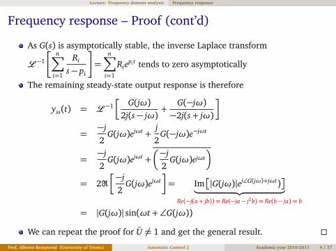
Example
G(s) =10(1+ s)
s2(1− 10s)(1+ 0.1s)
-40
Frequenza (rad/s)
Fa
se
(d
eg
)
M
od
ulo
(d
b)
-100
-50
0
50
100
10-2
10-1
1 10 102-200
-150
-100
-50
0
-60
-40
-60
For ω� 0.1: |G(jω)| ≈ 10ω2 (slope=-40 dB/dec), ∠G(jω)≈ −π
For ω= 0.1: 20 log1010ω2 = 60 dB
For 0.1<ω< 1: effect of unstable pole s= 0.1, decrease module by20 dB/dec, increase phase by π
2
For 1<ω< 10: effect of zero s= −1, +20 dB/dec module, +π2 phase
For ω> 10: effect of pole s= −10, -20 dB/dec module, -π2 phase
Prof. Alberto Bemporad (University of Trento) Automatic Control 2 Academic year 2010-2011 21 / 37

Lecture: Frequency domain analysis Bode
Summary table for drawing asymptotic Bode plots
magnitude phasestable real pole T > 0 −20 dB/dec −π/2unstable real pole T < 0 −20 dB/dec π/2stable real zero τ > 0 +20 dB/dec π/2unstable real zero τ < 0 +20 dB/dec −π/2pair of stable complex poles ζ > 0 −40 dB/dec −πpair of unstable complex poles ζ < 0 −40 dB/dec π
pair of stable complex zeros ζ′ > 0 +40 dB/dec π
pair of unstable complex zeros ζ′ < 0 +40 dB/dec −π
Prof. Alberto Bemporad (University of Trento) Automatic Control 2 Academic year 2010-2011 22 / 37

Lecture: Frequency domain analysis Bode
More on damped oscillatory modes
Let s= a± jb be complex poles, b 6= 0
Since (s− (a− jb))(s− (a+ jb)) = (s− a)2 + b2 = s2 − 2as+ (a2 + b2) =(a2 + b2)(1− 2a
a2+b2 s+ 1a2+b2 s2), we get
ωn =p
a2 + b2 = |a± jb|, ζ= −a
pa2 + b2
= − cos∠(a± jb)
Note that ζ > 0 if and only if a< 0
Vice versa, a= −ζωn, and b=ωn
p
1− ζ2
The natural response is
Me−ζωnt sin(ωn
p
1− ζ2t+φ)
where M, φ depend on the initial conditions
The frequency ωd =ωn
p
1− ζ2 is called damped natural frequency
Prof. Alberto Bemporad (University of Trento) Automatic Control 2 Academic year 2010-2011 23 / 37

Lecture: Frequency domain analysis Bode
Zero/pole/gain form and Bode form
Sometimes the transfer function G(s) is given in zero/pole/gain form (ZPK)
G(s) =K′
sh
Πi(s− zi)Πj(s− pj)
Πi
�
s2 + 2ζ′iω′nis+ω
′2ni
�
Πj
�
s2 + 2ζjωnjs+ω2nj
�
The relations between Bode form and ZPK form are
zi = −1τi
, pj = −1Ti
, K = K′Πi(−zi)Πiω
′2ni
Πj(−pj)Πiω2ni
MATLAB»zpk(G)
Prof. Alberto Bemporad (University of Trento) Automatic Control 2 Academic year 2010-2011 24 / 37

Lecture: Frequency domain analysis Nyquist plot
Nyquist (or polar) plot
Let G(s) be a transfer function of a linear time-invariant dynamical system
The Nyquist plot (or polar plot) is the graph in polar coordinates of G(jω) forω ∈ [0,+∞) in the complex plane
G(jω) = ρ(ω)ejφ(ω), where ρ(ω) = |G(jω)| and φ(ω) = ∠G(jω)
The Nyquist plot is one of the classical methods used in stability analysis oflinear systems
The Nyquist plot combines the Bode magnitude & phase plots in a single plot
Harry Nyquist
(1889–1976)
Prof. Alberto Bemporad (University of Trento) Automatic Control 2 Academic year 2010-2011 25 / 37

Lecture: Frequency domain analysis Nyquist plot
Nyquist plot
To draw a Nyquist plot of a transfer function G(s), we can give some hints:
−1 −0.8 −0.6 −0.4 −0.2 0 0.2 0.4 0.6 0.8 1−0.8
−0.6
−0.4
−0.2
0
0.2
0.4
0.6
0.80 dB
−20 dB
−10 dB
−6 dB−4 dB−2 dB
20 dB
10 dB
6 dB
4 dB 2 dB
Nyquist plot of G(s)
Real Axis
Imag
inar
y A
xis
G(s) =1
(1+ 0.1s)(1+ 0.002s+ 0.0001s2)
For ω= 0, the Nyquist plot equals the DCgain G(0)
If G(s) is strictly proper, limω→∞G(jω) = 0
In this case the angle of arrival equals(n−z − n+z − n−p + n+p )
π2 , where n+[−]z[p] is the #
of zeros [poles] with positive [negative] realpart
G(−jω) = G(jω)
A system without any zero with positive real part is called minimum phase
Prof. Alberto Bemporad (University of Trento) Automatic Control 2 Academic year 2010-2011 26 / 37

Lecture: Frequency domain analysis Nyquist criterion
Nyquist criterion
Consider a transfer function G(s) = N(s)/D(s) under unit static feedbacku(t) = −(y(t)− r(t))As y(t) = G(s)(−y(t) + r(t)), the closed-loop transfer function from r(t) to y(t)is
W(s) =G(s)
1+G(s)=
N(s)D(s) +N(s)
Nyquist stability criterion
The number NW of closed-loop unstable poles of W(s) is equal to thenumber NR of clock-wise rotations of the Nyquist plot around s= −1+ j0plus the number NG of unstable poles of G(s). [NW = NR +NG]
Corollary: simplified Nyquist criterion
For open-loop asympt. stable systems G(s) (NG = 0), the closed-loopsystem W(s) is asymptotically stable if and only if the Nyquist plot G(jω)does not encircle clock-wise the critical point −1+ j0. [NW = NR]
Prof. Alberto Bemporad (University of Trento) Automatic Control 2 Academic year 2010-2011 27 / 37

Lecture: Frequency domain analysis Nyquist criterion
Nyquist stability criterion
Proof:
Follows by the Argument principle: “The polar diagram of 1+G(s) has anumber of clock-wise rotations around the origin equal to the number ofzeros of 1+G(s) (=roots of N(s) +G(s)) minus the number of poles of1+G(s) (=roots of D(s)) of 1+G(s)”The poles of W(s) are the zeros of 1+G(s) �
Note: the number of counter-clockwise encirclements counts as a negativenumber of clockwise encirclementsUse of Nyquist criterion for open-loop stable systems:
1 draw the Nyquist plot of G(s)2 count the number of clockwise rotations around −1+ j03 if −1+ j0 is not encircled, the closed-loop system W(s) = G(s)/(1+G(s)) is stable
The Nyquist criterion is limited to SISO systems
Prof. Alberto Bemporad (University of Trento) Automatic Control 2 Academic year 2010-2011 28 / 37

Lecture: Frequency domain analysis Nyquist criterion
Example
Consider the transfer function G(s) =10
(s+ 1)2=
10s2 + 2s+ 1
under static output
feedback u(t) = −(y(t)− r(t))
−2 0 2 4 6 8 10−8
−6
−4
−2
0
2
4
6
8
Nyquist Diagram
Real Axis
Imagin
ary
Axis
MATLAB»G=tf(10,[1 2 1])»nyquist(G)
The closed-loop transfer function is
W(s) =G(s)
1+G(s)
The Nyquist plot of G(s) does not encircle−1+ j0
By Nyquist criterion, W(s) is asymptoticallystable
Prof. Alberto Bemporad (University of Trento) Automatic Control 2 Academic year 2010-2011 29 / 37

Lecture: Frequency domain analysis Nyquist criterion
Example
Consider the transfer function G(s) =10
s3 + 3s2 + 2s+ 1under unit output feedback
u(t) = −2(y(t)− r(t))
−10 −5 0 5 10 15 20−25
−20
−15
−10
−5
0
5
10
15
20
25
Nyquist Diagram
Real Axis
Imag
inar
y A
xis
MATLAB»G=tf(10,[1 3 2 1]); K=2»nyquist(K*G)»L=feedback(G,K)»pole(L)-3.87970.4398 + 2.2846i0.4398 - 2.2846i
The closed-loop transfer function is
W(s) =2G(s)
1+ 2G(s)
The Nyquist plot of 2G(s) encircles −1+ j0twice
By Nyquist criterion, W(s) is unstable
Prof. Alberto Bemporad (University of Trento) Automatic Control 2 Academic year 2010-2011 30 / 37

Lecture: Frequency domain analysis Nyquist criterion
Dealing with imaginary poles
The Nyquist plot is generated by a closed curve, the Nyquist contour, rotatingclock-wise from 0− j∞ to 0+ j∞ and back to 0− j∞ along a semi-circle ofradius∞, avoiding singularities of G(jω)We distinguish three types of curves, depending on the number of poles onthe imaginary axis:
Re(!)
Im(!)
x
+!j0
Wednesday, April 28, 2010
no poles on imaginary axis
Re(!)
Im(!)
x0+!
Wednesday, April 28, 2010
pole(s) in s= 0
(counted as stable)
Re(!)
Im(!)
x0+!
j!0
!j!0 x
x
!+0
!!+0
!!!0
!!0
Wednesday, April 28, 2010
pole(s) in s= ±jω
(counted as stable)Prof. Alberto Bemporad (University of Trento) Automatic Control 2 Academic year 2010-2011 31 / 37

Lecture: Frequency domain analysis Nyquist criterion
Stability analysis of static output feedback
Under static output feedback u(t) = −K(y(t)− r(t)), the closed-loop transferfunction from r(t) to y(t) is
W(s) =KG(s)
1+KG(s)
The number of encirclements of −1+ j0 of KG(s) is equal to the number ofencirclements of − 1
K + j0 of G(s)To analyze closed-loop stability for different values of K is enough to drawNyquist plot of G(s) and move the point − 1
K + j0 on the real axis
G(s) =60
(s2 + 2s+ 20)(s+ 1)
I0=no unstable closed-loop polesI2 =two unstable closed-loop polesI1=an unstable closed-loop pole
Prof. Alberto Bemporad (University of Trento) Automatic Control 2 Academic year 2010-2011 32 / 37

Lecture: Frequency domain analysis Phase and gain margins
Phase margin
Assume G(s) is open-loop asymptotically stableLet ωc be the gain crossover frequency, that is |G(jωc)|= 1To avoid encircling the point −1+ j0, we want the phase ∠G(jωc) as far awayas possible from −πThe phase margin is the quantity
Mp = ∠G(jωc)− (−π)
If Mp > 0, unit negative feedback control is asymptotically stabilizingFor robustness of stability we would like a large positive phase margin
Mp!G(j!)
!G(j!)
G(j!c)
!1 + j0
Wednesday, April 28, 2010
Prof. Alberto Bemporad (University of Trento) Automatic Control 2 Academic year 2010-2011 33 / 37

Lecture: Frequency domain analysis Phase and gain margins
Gain margin
Assume G(s) is open-loop asymptotically stableLet ωπ be the phase crossover frequency such that ∠G(jωπ) = −πTo avoid encircling the point −1+ j0, we want the point G(jωπ) as far aspossible away from −1+ j0.The gain margin is the inverse of |G(jωπ)|, expressed in dB
Mg = 20 log101
|G(jωπ)|= −|G(jωπ)|dB
For robustness of stability we like to have a large gain margin
1
Mg
!G(j!)
!G(j!)
!1 + j0
G(j!!)
Wednesday, April 28, 2010
Sometimes the gain margin isdefined as
Mg =1
|G(jωπ)|
and therefore G(jωπ) = −1
Mg+ j0
Prof. Alberto Bemporad (University of Trento) Automatic Control 2 Academic year 2010-2011 34 / 37

Lecture: Frequency domain analysis Phase and gain margins
Stability analysis using phase and gain margins
G(s) =8
s3 + 4s2 + 4s+ 2
The phase and gain margins help assessing the degree of robustness of aclosed-loop system against uncertainties in the magnitude and phase of theprocess model
They can be also applied to analyze the stability of dynamic output feedbacklaws u(t) = C(s)(y(t)− r(t)), by looking at the Bode plots of the loop functionC(jω)G(jω) (see next lecture on “loop shaping”)
Prof. Alberto Bemporad (University of Trento) Automatic Control 2 Academic year 2010-2011 35 / 37

Lecture: Frequency domain analysis Phase and gain margins
Stability analysis using phase and gain margins
However in some cases phase and gain margins are not good indicators, seethe following example
Mp
!G(j!)
!G(j!)
!1 + j0
Thursday, April 29, 2010
The system is characterized by a large phase margin, but the polar plot isvery close to the point (−1,0)The system is not very robust to model uncertainties changing G(s) from itsnominal value
In conclusion, phase and gain margins give good indications on how the loopfunction should be modified, but the complete Bode and Nyquist plots mustbe checked to conclude about closed-loop stability
Prof. Alberto Bemporad (University of Trento) Automatic Control 2 Academic year 2010-2011 36 / 37

Lecture: Frequency domain analysis Phase and gain margins
English-Italian Vocabulary
frequency response risposta in frequenzaangular frequency pulsazionesteady-state regime permanenteBode plot diagramma di BodeBode form forma di BodeBode gain guadagno di Bodesystem’s type tipo del sistematime constant costante di tempodamping ratio fattore di smorzamentonatural frequency frequenza naturalezero/pole/gain form forma poli/zeriminimum phase system sistema a fase minimaNyquist plot diagramma di Nyquistcrossover frequency frequenza di attraversamento
Translation is obvious otherwise.Prof. Alberto Bemporad (University of Trento) Automatic Control 2 Academic year 2010-2011 37 / 37