Automatic design of fiber-reinforced soft actuators for trajectory

ENG

INEE

RIN

G

Automatic design of fiber-reinforced soft actuatorsfor trajectory matchingFionnuala Connollya, Conor J. Walsha,b,1, and Katia Bertoldia,c,1

aHarvard John A. Paulson School of Engineering and Applied Sciences, Cambridge, MA 02138; bWyss Institute for Biologically Inspired Engineering, HarvardUniversity, Cambridge, MA 02138; and cKavli Institute, Harvard University, Cambridge, MA 02138

Edited by David A. Weitz, Harvard University, Cambridge, MA, and approved November 21, 2016 (received for review September 12, 2016)

Soft actuators are the components responsible for producingmotion in soft robots. Although soft actuators have allowed fora variety of innovative applications, there is a need for designtools that can help to efficiently and systematically design actua-tors for particular functions. Mathematical modeling of soft actu-ators is an area that is still in its infancy but has the potential toprovide quantitative insights into the response of the actuators.These insights can be used to guide actuator design, thus accel-erating the design process. Here, we study fluid-powered fiber-reinforced actuators, because these have previously been shownto be capable of producing a wide range of motions. We presenta design strategy that takes a kinematic trajectory as its inputand uses analytical modeling based on nonlinear elasticity andoptimization to identify the optimal design parameters for anactuator that will follow this trajectory upon pressurization. Weexperimentally verify our modeling approach, and finally wedemonstrate how the strategy works, by designing actuators thatreplicate the motion of the index finger and thumb.

soft robotics | fiber-reinforced actuators | customized actuators

In the field of robotics, it is essential to understand how todesign a robot such that it can perform a particular motion for

a target application. For example, this robot could be a robot armthat moves along a certain path or a wearable robot that assistswith motion of a limb. For conventional hard robots, methodshave been developed to describe the forward kinematics (i.e., forgiven actuator inputs, what will the configuration of the robotbe) and inverse kinematics (i.e., for a desired configuration ofthe robot, what should the actuator inputs be) (1–4).

Recently, there has been significant progress in the field ofsoft robotics, with the development of many soft grippers (5, 6),locomotion robots (7, 8), and assistive devices (9). Althoughtheir inherent compliance, easy fabrication, and ability to achievecomplex output motions from simple inputs have made softrobots very popular (10, 11), there is growing recognition thatthe development of methods for efficiently designing actuatorsfor particular functions is essential to the advancement of thefield. To this end, some research groups have begun focus-ing their efforts on modeling and characterizing soft actua-tors (12–20). In particular, significant progress has been madeon solving the forward kinematics problem (16–19) and evenon using dynamic modeling to perform motion planning (14).However, the practical problem of designing a soft actuatorto achieve a particular motion remains an issue. Finite ele-ment (FE) analysis has previously been used as a design toolto find the optimal geometric parameters for a soft pneumaticactuator, given some design criteria (15). Although this pro-cedure yields some nice results, only basic motions (linear orbending) were studied, because the method is computationallyintensive. An alternative approach is to use analytical modelingcombined with optimization to determine the properties of a softactuator that will achieve a particular motion for some targetapplication.

Here, we focus on fiber-reinforced actuators (17–21), andgiven a particular trajectory, we find the optimal design param-

eters for an actuator that will replicate that trajectory uponpressurization. To achieve this goal, we first use a nonlin-ear elasticity approach to derive analytical models that pro-vide a relationship between the actuator design parameters(geometry and material properties) and the actuator deforma-tion as a function of pressure for each motion type of inter-est (extending, expanding, twisting, and bending). Then, weuse optimization to determine properties for actuators thatmatch the desired trajectory (Fig. 1). Whereas similar actua-tors were previously designed empirically (22, 23), here, we pro-pose a robust and efficient strategy to streamline the designprocess. Furthermore, this strategy is not limited to the spe-cific cases presented here (namely the trajectories of the indexfinger and thumb) but, rather, could be applied to producerequired trajectories in a variety of soft robotic systems, suchas locomotion robots, assembly line robots, or devices for pipeinspection.

Analytical Modeling of Actuator SegmentsOur approach is based on assuming a desired actuator consists ofmultiple segments (mimicking the links and joints of the biologi-cal digit), where each different segment undergoes some combi-nation of axial extension, radial expansion, twisting about its axis,and bending upon pressurization. To realize actuators capableof replicating complex motions, we use segments consisting of acylindrical elastomeric tube surrounded by fibers arranged in ahelical pattern at a characteristic fiber angle α (Fig. 2A) (23, 24),because it has been shown that by varying the fiber angle andmaterials used, these segments can be easily tuned to achieve awide range of motions (17–21). When the elastomeric tube is ofuniform stiffness, the segment undergoes some combination of

Significance

Fluid-powered elastomeric soft robots have been shown tobe able to generate complex output motion using a simplecontrol input such as pressurization of a working fluid. Thiscapability, which mimics similar functions often found in biol-ogy, results from variations in mechanical properties of thesoft robotic body that cause it to strain to different degreeswhen stress is applied with the fluid. In this work, we outlinea mechanics- and optimization-based approach that enablesthe automatic selection of mechanical properties of a fiber-reinforced soft actuator to match the kinematic trajectoryof the fingers or thumb during a grasping operation. Thismethodology can be readily extended to other applicationsthat require mimicking or assisting biological motions.

Author contributions: F.C., C.J.W., and K.B. designed research; F.C. performed research;F.C. and K.B. analyzed data; and F.C., C.J.W., and K.B. wrote the paper.

The authors declare no conflict of interest.

This article is a PNAS Direct Submission.1To whom correspondence may be addressed. Email: [email protected] [email protected].

This article contains supporting information online at www.pnas.org/lookup/suppl/doi:10.1073/pnas.1615140114/-/DCSupplemental.

www.pnas.org/cgi/doi/10.1073/pnas.1615140114 PNAS | January 3, 2017 | vol. 114 | no. 1 | 51–56

mailto:[email protected]

mailto:[email protected]

http://www.pnas.org/lookup/suppl/doi:10.1073/pnas.1615140114/-/DCSupplemental

http://www.pnas.org/lookup/suppl/doi:10.1073/pnas.1615140114/-/DCSupplemental

http://www.pnas.org/cgi/doi/10.1073/pnas.1615140114

http://crossmark.crossref.org/dialog/?doi=10.1073/pnas.1615140114&domain=pdf

extension

twist

α1,L1

α2,L2

α3,L3

α4,L4

α6,L6

α5,L5

single pressure

inlet

input 2: complex kinematics

output: input 1: actuator models

A B

C

expansion

bending

Fig. 1. Designing an actuator that replicates a complex input motion.(A) Analytical models of actuator segments that can extend, expand, twist, orbend are the first input to the design tool. (B) The second input to the designtool is the kinematics of the desired motion. (C) The design tool outputs theoptimal segment lengths and fiber angles for replicating the input motion.

axial extension, radial expansion, and twisting about its axis uponpressurization (17–19). In contrast, when the tube is composedof two elastomers of different stiffness, pressurization producesa bending motion (25, 26).

Previous work has explored the design space of fiber-rein-forced actuators capable of extending, expanding, and twistingusing FE analysis (20) and kinematics and kinetostatics model-ing (17–19). Although these existing analytical models providegreat insight into the behavior of fiber-reinforced actuators, theyare restricted to exactly two sets of fibers (a set of fibers beingfibers arranged at the same angle).

Model 2: bending

isotropic core

thin anisotropic outer layer

Model 1: extension, expansion and twist

isotropic elastomer

reinforcement

simplify to

A B

SdZ

Ri

Rm

Ro

ri

rm

ro

θ

dz

Ro

dψ

dφ

Apply pressure

C

α

Rm

Ri

Fig. 2. Modeling a fiber-reinforced actuator. (A) The actuator consists of an elastomeric tube surrounded by an arrangement of fibers. In the model, thissystem is simplified to an isotropic tube, with an outer layer of anisotropic (but homogeneous) material. (B) Parameters for the analytical model of anextending, expanding, twisting actuator. (C) Parameters for the analytical model of a bending actuator.

Here, we use a nonlinear elasticity approach, which facilitatesmodeling actuators with an arbitrary number of sets of fibers.Rather than modeling the tube and the fibers individually, wetreat them as a homogeneous anisotropic material (27–29). Morespecifically, because the fibers are located on the outside of thetube and not dispersed throughout its thickness, we model theactuator as a hollow cylinder of isotropic incompressible hypere-lastic material (corresponding to the elastomer), surrounded bya thin layer of anisotropic material (corresponding to the fiberreinforcement), and impose continuity of deformation betweenthe two layers (Fig. 2A). The isotropic core has initial innerradius Ri and outer radius Rm , and the outer anisotropic layerhas initial outer radius Ro . The anisotropic material has a pre-ferred direction that is determined by the initial fiber orienta-tion S = (0, cosα, sinα). We define a deformation gradient F,from which we calculate the left Cauchy–Green deformation ten-sor B = FFT , the current fiber orientation s = FS, and the tensorinvariants I1 = tr(B) and I4 = s.s.

The inner and outer layers require different strain energyexpressions, so let W (in) be the strain energy for the isotropiccore and W (out) be the strain energy for the anisotropic outerlayer. For the isotropic core, we choose a simple incompress-ible neo-Hookean model, so that W (in) =µ/2(I1 − 3), with µdenoting the initial shear modulus. For the anisotropic layer,let W (out) be the sum of two components, W (out) = c1W

(iso) +

c2W(aniso), where W (iso) =µ/2(I1− 3) is the contribution from

the isotropic elastomeric matrix, W (aniso) is the contributionfrom the fibers, and c1 and c2 are the corresponding volume frac-tions. To derive a suitable expression for W (aniso), we consider asmall section of the helical fiber and model it as a rod subject toan axial load (SI Appendix, Fig. S5). It is trivial to show that thestrain energy density of the rod is (SI Appendix)

W (aniso) =E(√I4 − 1)

2

2, [1]

where E is its Young’s modulus. By slightly modifying the strainenergy, the above equations can easily be extended to accountfor more than one set of fibers. For example, to achieve a pureextending actuator, we might require two sets of fibers, with fiberorientations s1 and s2. In this case, the strain energy density is

W (aniso) =E(√I4 − 1)

2

2+

E(√I6 − 1)

2

2, [2]

where I4 = s1.s1 and I6 = s2.s2.

52 | www.pnas.org/cgi/doi/10.1073/pnas.1615140114 Connolly et al.

http://www.pnas.org/lookup/suppl/doi:10.1073/pnas.1615140114/-/DCSupplemental/pnas.1615140114.sapp.pdf



ENG

INEE

RIN

G

A

C

D

F

G

I

H

E

B

Fig. 3. Analytical predictions and experimental results for extending, twist-ing, and bending actuators. (A) Heat map illustrating the axial extension (λz)as a function of fiber angle and input pressure. (B) Front and bottom viewsof an extending actuator. (C) Comparison between analytical prediction andexperimental results. (D) Heat map illustrating the twist per unit length (τ )as a function of fiber angle and input pressure. (E) Front and bottom viewsof a twisting actuator. (F) Comparison between analytical prediction and

We can then use the strain energies to calculate the Cauchystresses, which take the form

σ(in) = 2W(in)1 B− pI [3]

σ(out) = 2W(out)1 B + 2W

(out)4 s1 ⊗ s1 + 2W

(out)6 s2 ⊗ s2 − pI,

[4]

where Wi = ∂W∂Ii

, I is the identity matrix, and p is a hydrostaticpressure (30).

To further simplify the analytical modeling, we decouple bend-ing from the other motions. In the following, we first introducean analytical model describing an extending, expanding, twistingactuator and then a model for a bending actuator.

Modeling Extension, Expansion, and Twist. When the elastomericpart of the actuator is of uniform stiffness, we assume that thetube retains its cylindrical shape upon pressurization, and theradii become ri , rm , and ro in the pressurized configuration(Fig. 2B). The possible extension, expansion, and twisting defor-mations are then described by (SI Appendix)

F =

Rrλz

0 00 r

Rrτλz

0 0 λz

, [5]

where R,Φ,Z and r , φ, z are the radial, circumferential, andlongitudinal coordinates in the reference and current configura-tions, respectively (28, 31). Moreover, λz and τ denote the axialstretch and the twist per unit length, respectively. To determinethe current actuator configuration, we first apply the Cauchyequilibrium equations, obtaining

P =

∫ rm

ri

σ(in)φφ − σ

(in)rr

rdr +

∫ ro

rm

σ(out)φφ − σ(out)

rr

rdr , [6]

where P is the applied pressure. Assuming there are no externalaxial forces or external axial moments applied to the tube, theaxial load, N , and axial moment, M , are given by

N = 2π

∫ rm

ri

σ(in)zz rdr + 2π

∫ ro

rm

σ(out)zz rdr = Pπr2i [7]

and

M = 2π

∫ rm

ri

σ(in)φz r2dr + 2π

∫ ro

rm

σ(out)φz r2dr = 0. [8]

Eqs. 6–8 with the Cauchy stress σ as given in Eqs. 3 and 4 andthe deformation gradient of Eq. 5 are then solved to find λz , ri ,and τ as functions of P (SI Appendix).

Modeling Bending. Because the exact solution for the finite bend-ing of an elastic body is only possible under the assump-tion that the cross-sections of the cylinder remain planar uponpressurization—a condition that is severely violated by ouractuator—we assume (i) that the radial expansion can beneglected (i.e., r/R = 1) and (ii) vanishing stress in the radialdirection (i.e., σrr = 0). Note that these conditions are closelyapproximated when the actuator has fiber angle less than 30◦ andthe actuator walls are thin (16). Furthermore, because the actu-ators have a symmetric arrangement of fibers, no twisting takesplace, so the deformation gradient reduces to (SI Appendix)

F =

λz (φ)−1 0 00 1 00 0 λz (φ)

. [9]

experimental results. (G) Heat map illustrating the bend per unit length (ω)as a function of fiber angle and input pressure. (H) Front view of a bend-ing actuator. (I) Comparison between analytical prediction and experimen-tal results.

Connolly et al. PNAS | January 3, 2017 | vol. 114 | no. 1 | 53




Because the actuator bends due to the moment created bythe internal pressure acting on the actuator caps (SI Appendix,Fig. S9), we equate this moment

Mcap = 2PR2i

∫ π

0

sin2 φabs(Ri cos φ− Ri cosφ

)dφ, [10]

with the opposing moment due to the stress in the material

Mmat =

∫ ∫λ−1z σzz (Ri + τ)

(Ri cos φ− (Ri + τ) cosφ

)dφdτ,

[11]

where φ denotes the location of the neutral bending axis, dτ isthe differential wall thickness element, and dφ is the circumfer-ential angle element (Fig. 2C).

Now solving Mmat =Mcap yields the relationship betweeninput pressure and output bend angle:

P =

∫∫λ−1z σzz (Ri + τ)

(Ro cos φ− (Ri + τ) cosφ

)dφdτ

2R2i

∫ π0

sin2 φabs(Ri cos φ− Ri cosφ)dφ,

[12]

where σzz can be obtained by substituting F into Eqs. 3 and 4(SI Appendix).

Comparing Analytical and Experimental Results. To fabricate theextending, expanding, twisting actuators, we used the elastomerSmooth-Sil 950 (µ2 = 680 kPa; Smooth-On), and for the bend-ing actuators, we used both Smooth-Sil 950 and Dragon Skin 10(µ2 = 85 kPa; Smooth-On). The fiber reinforcement was Kevlar,with a Young’s modulus E = 31,067 MPa and radius r =0.0889 mm. Each actuator had an inner radius of 6.35 mm, wallthickness of 2 mm, and length of 160 mm. The effective thicknessof the fiber layer (8.89× 10-4 mm) is a fitting parameter here andwas identified using the results in SI Appendix, Fig. S7.

For the bending model, we used an FE simulation (SIAppendix, Fig. S10) to determine the location of the neutral axis(φ= 35◦). Using FE analysis, we determined that our bendingmodel was accurate for thin-walled actuators (SI Appendix, Fig.S11). However, for thicker-walled actuators, the model yieldedlower than expected bend angles at any given pressure. Tosolve this problem, we used one FE simulation (with fiber angleα= ±5◦) to determine an effective shear modulus µ (78 kPa)for the actuator (rather than using the shear moduli µ1 andµ2). We found that using this fitting parameter, we could accu-rately predict the response for actuators with other fiber angles(SI Appendix). Note that because FE analysis generally providesmore accurate results than our analytical bending model, analternative solution would be to use FE simulations to build adatabase of simulation results for actuators with a range of dif-ferent fiber angles. However, this option would be more compu-tationally expensive, and so, although not ideal, it is preferablein our case to use just one FE simulation to identify the fittingparameters for the analytical bending model, rather than relyingsolely on FE.

We first consider extending actuators (with two sets of fibers,arranged symmetrically). Fig. 3A shows how the amount of exten-sion undergone (illustrated by the color) depends on the fiberangle of the actuator (y axis) and the current actuation pressure(x axis). We see that an actuator with fiber angleα= 0◦ yields themost extension, whereas, in contrast, actuators with larger fiberangles undergo contraction. We fabricated and tested an actua-tor with fiber angles α= ±3◦ (highlighted in red in Fig. 3A), andthe results (Fig. 3 B and C) show good agreement between themodel and the experiment. Second, we consider twisting actu-ators, which have only one set of fibers. From Fig. 3D, we cansee that an actuator with fiber angle around 30◦ produces themaximum amount of twist per unit length. Fig. 3 E and F shows

that the analytical model accurately represents the twist per unitlength undergone by an actuator with fiber angle α= 3◦.

Finally, Fig. 3G illustrates the bend angle per unit length as afunction of fiber angle and actuation pressure. At any given pres-sure, for larger fiber angles, we see less bend per unit length.Comparing analytical and experimental results for a bendingactuator with fiber angles α= ±5◦ (Fig. 3 H and I), we see agood match between the model and the experiment.

Replicating Complex MotionsWe have presented two analytical models, which describe extend-ing, expanding, twisting, and bending actuator motions. In addi-tion to using these models to explore the actuator design space,we can use them for more complex operations, such as design-ing a single-input, multisegment actuator that follows a spe-cific trajectory. In the following sections, we will demonstratethis methodology by determining the properties of multisegmentactuators that can replicate finger and thumb motion.

The target motion of the actuator was determined using elec-tromagnetic trackers that were placed on the hand at the wrist,at each joint along the finger, and at the fingertip (SI Appendix,Fig. S13) (22). Time series data of the coordinates of each sensorin 3D space were recorded as the hand was opened and closed.Using these data, the configuration of the fingers and thumb dur-ing a grasping motion can be obtained. Adjacent sensors areconnected by links, and we use the data to calculate the lengthof each link and the angles between the links at each time. Wesmooth the data by applying a Savitzky–Golay filter. Since it willnot be possible to produce an actuator that will match the finger

extending segmentsbending segments

input

initialize design

variables

calculate required segment

update design

variables

fabricate actuator

objective function (Eq 13)

minimized?

yes

no

pressure P(j)

length lext,i twist angle θi

pressure P(j)

pressure P(j)

bend angle ψi

use analytical models

input:

output:

extending twisting bending

compare to:

Ŷ Ŷ Ŷ(j)

(j)

lext,i( j) θi

(j) P(j)

(j)

ltw,1

llink,1(j)Ψ1

Ψ2

θ

llink,2llink,3

(j)

( j)

lbend,1

(j)

lbend,2(j)

lbend,3(j)

lext,1(j)

lext,2

lext,3(j)

( j)

( j)

( j)

( j)Ψ3

twisting segments

(j)

αi αi αilext,i(0) ltw,i

(0) lbend,i(0)

ŶŶ Ŷ

Ŷ

Ŷ

Ŷ

ŶŶ

Ŷ

Ŷ

Fig. 4. Optimization algorithm for actuator design.














ENG

INEE

RIN

G

A C D

B

E

F H I

G

J

Fig. 5. (A and B) Finger actuator: qualita-tive comparison of actuator motion and fingermotion. (C) Comparison of input finger trajec-tory and output actuator trajectory. (D) Illustra-tion of segment lengths and fiber angles. (E)Quantitative comparison of desired, expected,and achieved link lengths (Left) and bend angles(Right). (F and G) Thumb actuator: qualita-tive comparison of actuator motion and thumbmotion. (H) Comparison of input thumb trajec-tory and output actuator trajectory. (I) Illustra-tion of segment lengths and fiber angles. (J)Quantitative comparison of desired, expected,and achieved twist angles (Left), link lengths(Center), and bend angles (Right).

trajectory exactly at every point, we choose just four configura-tions to match. (These configurations are equally spaced alongthe trajectory; SI Appendix, Figs. S14 and S15.) Because the inputdata represent the motion of the top of the finger, the top of theactuator we design should mimic the input motion.

The actuator will consist of multiple segments, each with a dif-ferent length and fiber angle. We prescribe the number of seg-ments and the type of each segment. (For replicating finger andthumb motion, expanding segments are not required, so eachsegment type is extend, bend, or twist.) The radius, wall thick-ness, and material parameters are the same as in the previoussection. (Here, we use Dragon Skin 10 for the extending andtwisting segments.) We set the maximum allowed pressure to80 kPa. (At higher pressures, the Matlab solver fsolve is unable tosolve Eqs. 6–8.) Furthermore, to simplify the fabrication proce-dure, we impose a minimum fiber angle of 5◦. Also, we prescribea maximum allowed fiber angle of 50◦, because above this angle,the radial expansion of the actuators becomes significant (20).Note that for a finger, bending occurs at discrete joints, but forthe actuator, it will of course take place over some finite length.To approximate the motion of the finger as closely as possible, wewant this length to be as short as possible, so we impose a max-

imum allowed bending segment length of 30 mm (SI Appendix).We then input all of this information, together with the mod-els we developed in the previous sections, into a nonlinear least-squares optimization algorithm in Matlab (lsqnonlin) (Fig. 4). Tofind the design parameters for an actuator that will move throughthe given configurations (combinations of link lengths and bendangles) as it is pressurized, we minimize

f = c1∑N

j=1

∑ntw

i=1

∣∣∣θ(j)i − θ(j)i

∣∣∣2 +∑N

j=1

∑next

i=1

∣∣∣l (j)ext,i − l(j)ext,i

∣∣∣2+ c2

∑N

j=1

∑nbend

i=1

∣∣∣P (j)i − P (j)

∣∣∣2, [13]

where ntw , next , and nbend are the total numbers of twisting,extending, and bending segments, respectively, and N is thenumber of goal configurations. The first term measures the dif-ference between the required (θ) and achieved (θ) twist angles;the second term measures the difference between the required(lext ) and achieved (lext ) segment lengths, and the third termmeasures the difference between the pressures at which therequired bend angles should be achieved (P) and the pressuresat which the required bend angles are actually achieved with

Connolly et al. PNAS | January 3, 2017 | vol. 114 | no. 1 | 55



the current set of variables (P). The parameters c1 = 100 andc2 = 1,000 are weights that balance the relative importance ofthe twisting, bending, and extending segments. If f is not suf-ficiently small, the variables are updated and the optimizationloop repeats. When the minimum value of f is found, the opti-mization outputs (i) the fiber angle αi for each segment, (ii) theinitial length of each of the bending and twisting segments, and(iii) the pressures P (j) at which the goal configurations will occur.

Index Finger Motion. The fiber angles and lengths required to imi-tate the movement of the index finger are illustrated in Fig. 5D.Segments 1, 3, and 6 have length 70 mm, 22 mm, and 15 mm,with fiber angles of ±40◦, ±50◦, and ±50◦, respectively. Thesesegments undergo axial contraction when pressurized. Segments2, 4, and 5 are bending segments of length 22 mm, 28 mm, and15 mm, with fiber angles of ±6◦, ±5◦ and ±5◦, respectively.

We fabricate the actuator as detailed in SI Appendix. To com-pare the actual performance of the actuator to the expected per-formance, we characterize it by taking pictures of the actuator atvarious different actuation pressures. We evaluate its motion byusing Matlab to track points on the actuator. We see good agree-ment between expected and actual motion (Fig. 5 C and E andMovie S1), with some discrepancies that are most likely due todefects in the actuator fabrication (for example, segment lengthsbeing up to 4 mm shorter than expected, due to the fibers beingwound around the actuator between segments; SI Appendix).

Thumb Motion. As a second example, we consider the design ofan actuator that upon pressurization, replicates the motion of athumb. The motion of the thumb is more complex than that ofthe finger, because it moves out of plane. We capture this out-of-plane motion as a twisting motion. We calculate the amountof twist by fitting a plane to the twisting links at each time andthen finding the angle between the normal to this plane and thenormal to the initial plane.

Fig. 5I illustrates the fiber angles that are needed to repro-duce the motion of the thumb, as predicted by the model. Seg-ment 1 is a twisting segment of length 25 mm, with fiber angle5◦; segments 2, 4, and 6 are bending segments of length 15 mm,

30 mm, and 22 mm, each with fiber angles ±5◦; and segments3, 5, and 7 are extending segments of length 20 mm, 8 mm, and17 mm, with fiber angles ±41◦, ±50◦, and ±47◦. To analyze themotion of this actuator, we placed two cameras at right anglesto each other and took pictures of the actuator at various differ-ent actuation pressures. The images were combined to reproducethe 3D motion of the actuator (SI Appendix). Fig. 5 H and J com-pares the input thumb kinematics and the output actuator motion(Movie S2). We see reasonable agreement between the expectedand achieved motions, with discrepancies in this case most likelydue to inaccuracies in measuring the actuator motion (for exam-ple, misalignment of cameras), as well as defects in actuator fab-rication (such as nonuniform wall thickness).

ConclusionsUsing analytical models for fiber-reinforced actuators thatextend, expand, twist, and bend, we have devised a method ofdesigning actuators customized for a particular function. Giventhe kinematics of the required motion, and the number andtype of segments required, the algorithm outputs the appro-priate length and fiber angle of each segment, thereby pro-viding a recipe for how the actuator should be made. Theprocedure is somewhat limited in its current form because itrequires the user to input the type of segments required, butfuture versions will eliminate the need for this step, thus fur-ther automating the procedure. Future work will also focus ondeveloping a model that combines bending with other motions,to increase the versatility of the algorithm. The design tool wehave presented here has immense potential to streamline andaccelerate the design of soft actuators for a particular task,eliminating much of the trial and error procedure that is cur-rently used and broadening the scope of fiber-reinforced softactuators.

ACKNOWLEDGMENTS. The authors thank Dr. J. Weaver for assistance with3D printing and Dr. P. Polygerinos and Dr. S. Sanan for helpful discussions.This work was partially supported by National Science Foundation Grant1317744, the Materials Research Science and Engineering Center underNational Science Foundation Award DMR-1420570, the Wyss Institute, andHarvard’s Paulson School of Engineering and Applied Sciences.

1. Denavit J, Hartenberg RS (1955) A kinematic notation for lower pair mechanismsbased on matrices. J Appl Mech 22:215–221.

2. Murray RM, Li Z, Sastry SS (1994) A Mathematical Introduction to Robotic Manipula-tion (CRC Press, Boca Raton, FL).

3. Aristidou A, Lasenby J (2009) Inverse Kinematics: A Review of Existing Techniques andIntroduction of a New Fast Iterative Solver (University of Cambridge, Cambridge, UK).

4. Colome A, Torras C (2012) Redundant inverse kinematics: Experimental comparativereview and two enhancements (IEEE/RSJ Int Conf Intell Robot Syst, Vilamoura, Portu-gal), pp 5333–5340.

5. Suzumori K, Iikura S, Tanaka H (1992) Applying a flexible microactuator to roboticmechanisms. IEEE Control Syst 12(1):21–27.

6. Martinez RV, et al. (2013) Robotic tentacles with three-dimensional mobility based onflexible elastomers. Adv Mater 25(2):205–212.

7. Marchese AD, Onal CD, Rus D (2014) Autonomous soft robotic fish capable of escapemaneuvers using fluidic elastomer actuators. Soft Robot 1(1):75–87.

8. Tolley MT, et al. (2014) A resilient, untethered soft robot. Soft Robot 1(3):213–223.9. Connelly L, et al. (2009) Use of a pneumatic glove for hand rehabilitation following

stroke. Conf Proc IEEE Eng Med Biol Soc 2009:2434–2437.10. Rus D, Tolley MT (2015) Design, fabrication and control of soft robots. Nature

521(7553):467–475.11. Majidi C (2013) Soft robotics: a perspective - current trends and prospects for the

future. Soft Robot 1(1):5–11.12. Hirai S, et al. (2000) Qualitative synthesis of deformable cylindrical actuators through

constraint topology. IEEE/RSJ Int Conf Intell Robot Syst1:197–202.13. Case JC, White EL, Kramer RK (2015) Soft material characterization for robotic appli-

cations. Soft Robot 2(2):80–87.14. Marchese AD, Tedrake R, Rus D (2016) Dynamics and trajectory optimization for a soft

spatial fluidic elastomer manipulator. Int J Rob Res 35(8):1000–1019.15. Moseley P, et al. (2016) Modeling, design, and development of soft pneumatic actua-

tors with finite element method. Adv Eng Mater 18(6):978–98816. Polygerinos P, et al. (2015) Modeling of soft fiber-reinforced bending actuators. IEEE

Trans Robot 31(3):778–789.

17. Singh G, Krishnan G (2015) An isoperimetric formulation to predict deformationbehavior of pneumatic fiber reinforced elastomeric actuators (IEEE/RSJ Int Conf IntellRobot Syst, Hamburg, Germany), pp 1738–1743.

18. Krishnan G, Bishop-Moser J, Kim C, Kota S (2015) Kinematics of a generalized class ofpneumatic artificial muscles. J Mech Robot 7(4):041014.

19. Bishop-Moser J, Kota S (2015) Design and modeling of generalized fiber-reinforcedpneumatic soft actuators. IEEE Trans Robot 31(3):536–545.

20. Connolly F, Polygerinos P, Walsh CJ, Bertoldi K (2015) Mechanical programming ofsoft actuators by varying fiber angle. Soft Robot 2(1):26–32.

21. Galloway KC, Polygerinos P, Walsh CJ, Wood RJ (2013) Mechanically programmablebend radius for fiber-reinforced soft actuators (Int Conf Adv Robot, Montevideo,Uruguay), pp 1–6.

22. Polygerinos P, Wang Z, Galloway KC, Wood RJ, Walsh CJ (2015) Soft robotic glove forcombined assistance and at-home rehabilitation. Rob Auton Syst 73:135–143.

23. Galloway K, et al. (2015) Multi-segment reinforced actuators and applications. USPatent WO 2015066143 A1.

24. Bishop-Moser J, Krishnan G, Kota S (2015) Fiber-reinforced actuator. US Patent US20150040753 A1.

25. Suzumori K, Iikura S, Tanaka H (1991) Flexible microactuator for miniature robots(Proc IEEE Micro Electro Mech Syst, Nara, Japan), pp 204–209.

26. Firouzeh A, Salerno M, Paik J (2015) Soft pneumatic actuator with adjustable stiff-ness layers for multi-DoF actuation (IEEE/RSJ Int Conf Intell Robot Syst, Hamburg,Germany), pp 1117–1124.

27. Adkins JE, Rivlin RS (1955) Large elastic deformations of isotropic materials X. Rein-forcement by inextensible cords. Philos Trans R Soc Lond A 248(944):201–223.

28. Kassianidis F (2007) Boundary-value problems for transversely isotropic hyperelasticsolids. PhD Thesis (University of Glasgow, Glasgow, UK).

29. Goriely A, Tabor M (2013) Rotation, inversion, and perversion in anisotropic elasticcylindrical tubes and membranes. Proc Math Phys Eng Sci 469(2153):20130011.

30. Holzapfel GA (2000) Nonlinear Solid Mechanics. A Continuum Approach for Engineer-ing (Wiley, Chichester, NY).

31. Ogden RW (1984) Non-Linear Elastic Deformations (Dover, New York).



http://movie-usa.glencoesoftware.com/video/10.1073/pnas.1615140114/video-1



http://movie-usa.glencoesoftware.com/video/10.1073/pnas.1615140114/video-2


SI Appendix for

Automatic design of fiber-reinforced soft actuators for

trajectory matching

Fionnuala Connolly∗, Conor J. Walsh∗,†, Katia Bertoldi∗,‡

∗Harvard John A. Paulson School of Engineering and Applied Sciences, Cambridge, MA 02138

†Wyss Institute, Harvard University, Cambridge, MA 02138

‡Kavli Institute Harvard University, Cambridge, MA 02138

S1 Actuator fabrication and material characterization

In this section, we describe our methods for fabricating fiber-reinforced soft actuators. We first describe

how to fabricate actuators which extend, expand, and twist, then actuators which bend, and finally,

segmented actuators. We describe our procedure for molding the elastomeric tube, and for winding the

fibers at a particular angle. We also describe the procedure for characterizing the elastomers used.

1

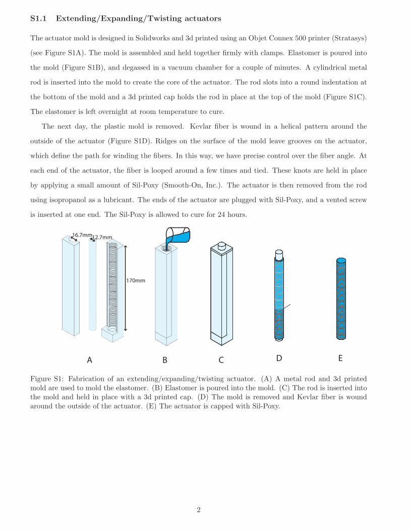
S1.1 Extending/Expanding/Twisting actuators

The actuator mold is designed in Solidworks and 3d printed using an Objet Connex 500 printer (Stratasys)

(see Figure S1A). The mold is assembled and held together firmly with clamps. Elastomer is poured into

the mold (Figure S1B), and degassed in a vacuum chamber for a couple of minutes. A cylindrical metal

rod is inserted into the mold to create the core of the actuator. The rod slots into a round indentation at

the bottom of the mold and a 3d printed cap holds the rod in place at the top of the mold (Figure S1C).

The elastomer is left overnight at room temperature to cure.

The next day, the plastic mold is removed. Kevlar fiber is wound in a helical pattern around the

outside of the actuator (Figure S1D). Ridges on the surface of the mold leave grooves on the actuator,

which define the path for winding the fibers. In this way, we have precise control over the fiber angle. At

each end of the actuator, the fiber is looped around a few times and tied. These knots are held in place

by applying a small amount of Sil-Poxy (Smooth-On, Inc.). The actuator is then removed from the rod

using isopropanol as a lubricant. The ends of the actuator are plugged with Sil-Poxy, and a vented screw

is inserted at one end. The Sil-Poxy is allowed to cure for 24 hours.

16.7mm12.7mm

170mm

A B C D E

Figure S1: Fabrication of an extending/expanding/twisting actuator. (A) A metal rod and 3d printedmold are used to mold the elastomer. (B) Elastomer is poured into the mold. (C) The rod is inserted intothe mold and held in place with a 3d printed cap. (D) The mold is removed and Kevlar fiber is woundaround the outside of the actuator. (E) The actuator is capped with Sil-Poxy.

2

S1.2 Bending actuators

The fabrication procedure for bending actuators is similar to the procedure for extending/expanding/twisting

actuators. The only difference is that the cylindrical tube is composed of two different elastomers. To

fabricate the first half of this tube, one side of the 3d printed mold is laid down flat, and Elastomer 1

is poured into the mold (Figure S2A). The metal rod is placed on top of the elastomer, and slots into

place at the top and bottom of the mold. This is left to cure overnight in a pressure chamber (curing at

high pressure reduces the size of any air bubbles present in the elastomer). The next day, the edges of

the elastomer are trimmed (without removing it from the mold) so that it forms a perfect half-cylinder.

Elastomer 2 (of different stiffness to Elastomer 1) is poured on top of the metal rod (Figure S2B), and the

top half of the mold is quickly placed on top. The two halves of the mold are held together firmly with

clamps. Again, this is left overnight in a pressure chamber to allow the second elastomer to cure (Figure

S2C). The remainder of the procedure is the same as for the extending/expanding/twisting actuators.

A

B

C D E

Figure S2: Fabrication of a bending actuator (A) The first half of the mold is laid down flat and Elastomer1 is poured in. (B) When Elastomer 1 has cured, Elastomer 2 is poured on top. (C) The second half ofthe mold is placed on top and Elastomer 2 is left to cure. (D) The mold is removed and Kevlar fiber iswound around the outside of the actuator. (E) The actuator is capped with Sil-Poxy.

3

S1.3 Segmented actuators

A segmented actuator consists of some bending actuator segments and some extending/twisting actuator

segments. One half of the actuator is made entirely of Elastomer 1. The other half is made of Elastomer 1

if it is a twisting and/or extending segment, and Elastomer 2 (different stiffness) if it is a bending segment.

Therefore, a segmented mold is used, as shown in Figure S3A.

First, the whole mold is assembled and held together with clamps, and the actuator is cast entirely from

Elastomer 1 (Figure S3B,C). Then one side of the mold (the segmented side) is removed. The segments

are then fabricated one by one. As shown in Figure S3D,E, the exposed elastomer is cut away, and the

new elastomer is poured (Elastomer 1 or 2, depending on the type of segment). The elastomer is cut away

segment by segment like this so that every time new elastomer is being poured, it is being poured on a

freshly exposed surface. This improves the bond between the elastomers. To speed up the process, the

elastomer is cured in the oven for 30 minutes at 60◦C (rather than overnight at room temperature). When

all of the segments have cured, the mold is removed, and fibers are wrapped around the outside of the

actuator.

A B C D

E

F G H

X-ACTO

Figure S3: Fabrication of a segmented actuator. (A) A metal rod and 3d printed mold are used to moldthe elastomer. (B) First, Elastomer 1 is used to make the entire actuator. (C) Elastomer 1 is left to cure.(D)-(G) The elastomeric segments are fabricated one by one. (H) The mold is removed and the actuatoris capped with Sil-Poxy.

4

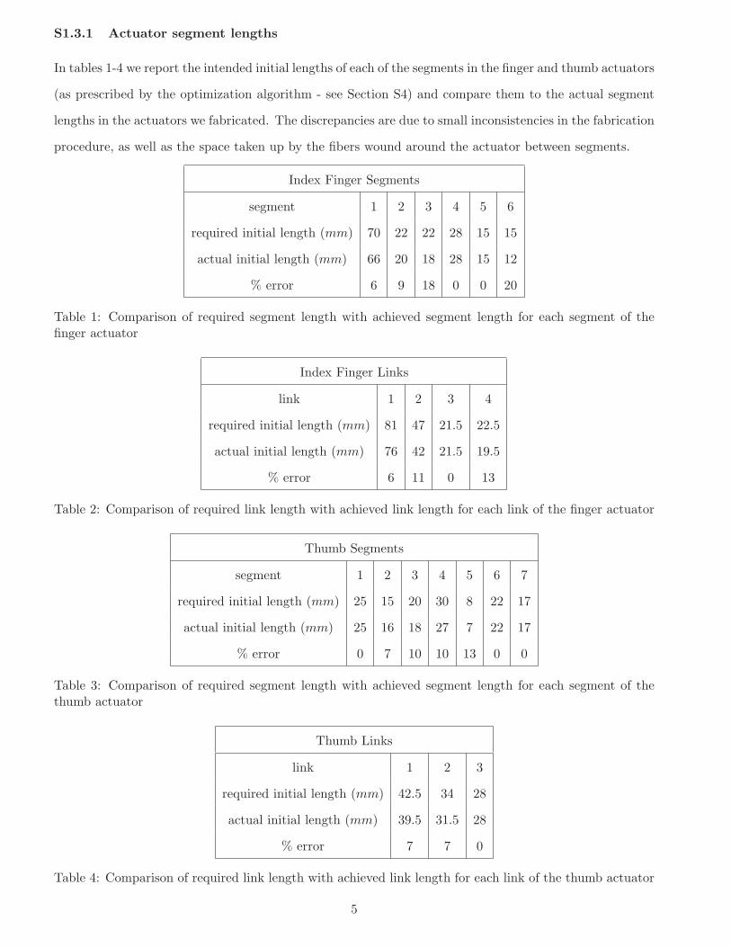
S1.3.1 Actuator segment lengths

In tables 1-4 we report the intended initial lengths of each of the segments in the finger and thumb actuators

(as prescribed by the optimization algorithm - see Section S4) and compare them to the actual segment

lengths in the actuators we fabricated. The discrepancies are due to small inconsistencies in the fabrication

procedure, as well as the space taken up by the fibers wound around the actuator between segments.

Index Finger Segments

segment 1 2 3 4 5 6

required initial length (mm) 70 22 22 28 15 15

actual initial length (mm) 66 20 18 28 15 12

% error 6 9 18 0 0 20

Table 1: Comparison of required segment length with achieved segment length for each segment of thefinger actuator

Index Finger Links

link 1 2 3 4

required initial length (mm) 81 47 21.5 22.5

actual initial length (mm) 76 42 21.5 19.5

% error 6 11 0 13

Table 2: Comparison of required link length with achieved link length for each link of the finger actuator

Thumb Segments

segment 1 2 3 4 5 6 7

required initial length (mm) 25 15 20 30 8 22 17

actual initial length (mm) 25 16 18 27 7 22 17

% error 0 7 10 10 13 0 0

Table 3: Comparison of required segment length with achieved segment length for each segment of thethumb actuator

Thumb Links

link 1 2 3

required initial length (mm) 42.5 34 28

actual initial length (mm) 39.5 31.5 28

% error 7 7 0

Table 4: Comparison of required link length with achieved link length for each link of the thumb actuator

5

S1.4 Material Characterization

Dogbone-shaped samples (ASTM standard) made out of the elastomers used to fabricate the actuators

(Smooth-Sil 950 and Dragon Skin 10, Smooth-on Inc., PA, USA) were tested under uniaxial tension using

a single-axis Instron (model 5566; Instron, Inc.) with a 100N load cell. The material behavior up to a

stretch of 2.5 is reported in Figure S4. We used a least squares method to fit an incompressible Neo-

Hookean model to the measured data, and found that the material response is best captured with an

initial shear modulus µ = 0.085 MPa for Dragon Skin 10 and µ = 0.68 MPa for Smooth-Sil 950.

λ

1 1.5 2 2.5

σ (

MP

a)

0

0.5

1

DS10 exp

DS10 !t, µ=0.085MPa

SmoothSil exp

SmoothSil !t, µ=0.68MPa

Figure S4: Experimental stress-strain data and a best-fit neo-Hookean model for Dragonskin 10 andSmoothSil 950 under uniaxial tensile loading

S2 Finite Element Simulations

As well as performing experiments, we performed finite element simulations as additional verification

for our analytical modeling. All finite element simulations were carried out using the commercial finite

element software Abaqus (SIMULIA, Providence, RI). In each case, the elastomer was modeled as an

incompressible neo-Hookean material. The Kevlar fibers were modeled as a linearly elastic material using

the manufacturer’s specifications: diameter 0.1778mm, Young’s modulus 31.067 × 106kPa and Poisson’s

ratio 0.36. For the elastomer, 20-node quadratic brick elements, with reduced integration (Abaqus ele-

ment type C3D20R) were used, and 3-node quadratic beam elements (Abaqus element type B32) were

used for the fibers. Perfect bonding between the fibers and the elastomer was assumed (the fibers were

connected to the elastomer by tie constraints). Quasi-static non-linear simulations were performed using

Abaqus/Standard. One end of the actuator was held fixed, and a pressure load was applied to the inner

surface of the actuator.

Note that sample files for running Abaqus simulations can be found on softroboticstoolkit.com.

6

S3 Analytical modeling

In this section, we present analytical models for fiber-reinforced actuators which extend, expand, twist,

and bend. We use a non-linear elasticity approach to analytically model the response of the fiber-reinforced

actuators free to deform under pressurization. Rather than modeling the tube and the fibers individually,

we treat them as a homogeneous anisotropic material [1-3]. More specifically, as the fibers are located on

the outside of the tube and not dispersed throughout its thickness, we model the actuator as a hollow

cylinder of isotropic incompressible hyperelastic material (corresponding to the elastomer), surrounded by

a thin layer of anisotropic material (corresponding to the fiber reinforcement), and impose continuity of

deformation between the two layers (Figure 2A of the main text). The isotropic core has initial inner ra-

dius Ri and outer radius Rm, while the outer anisotropic layer has initial outer radius Ro. The anisotropic

material has a preferred direction which is determined by the initial fiber orientation S = (0, cosα, sinα),

where α is the fiber angle.

In the following, we first construct the strain energy expressions for both the inner and outer layers.

Then, to simplify the analytical modeling, we decouple bending from the other motions, so we first intro-

duce a model for actuators which extend, expand, and twist upon pressurization, followed by a model for

actuators which bend upon pressurization. In each case, we use experimental and finite element results to

validate the analytical models.

S3.1 Strain energy for the actuators

The inner and outer layers require different strain energy expressions, so let W (in) be the strain energy for

the isotropic core, and W (out) be the strain energy for the anisotropic outer layer. For the isotropic core,

we choose a simple incompressible neo-Hookean model, so that

W (in) =µ

2(I1 − 3), (S1)

µ denoting the initial shear modulus and I1 = tr(FFT ), F being the deformation gradient. For the

anisotropic layer, let W (out) be the sum of two components,

W (out) = c1W(iso) + c2W

(aniso), (S2)

where W (iso) = µ/2(I1 − 3) is the contribution from the isotropic elastomeric matrix, W (aniso) is the

contribution from the fibers, and ci are the corresponding volume fractions. To derive a suitable expression

for W (aniso), we consider a helical fiber with cross-sectional area a, initial orientation S = (0, cosα, sinα),

7

and current orientation s = FS subject to an axial load F (Figure S5A). We focus on a small segment of the

helical fiber of length dl which undergoes a change in length dx. Assuming there is a linear relationship

between the force F and extension dx (as shown in Figure S5B), the strain energy for the segment,

dW (fiber), is equal to the area underneath the force-displacement curve,

dW (fiber) =1

2Fdx. (S3)

For the considered linear elastic fiber F can be expressed as

F = Eǫa (S4)

where ǫ = dx/dl is the axial strain, and E is the Young’s modulus. Substituting Equation (S4) into

Equation (S3), we have

dW (fiber) =1

2ǫEadx =

1

2ǫ2Eadl, (S5)

and integrating yields

W (fiber) =

∫ Lf

0

1

2ǫ2Eadl =

1

2ǫ2EaLf , (S6)

which is the energy of the helical fibers. Since I4 = s.s is the stretch of the fiber, we have ǫ =√I4 − 1,

and substituting this in Equation (S6) yields

W (fiber) =(√I4 − 1)2EaLf

2(S7)

Dividing by the volume of the fiber yields the strain energy density

W (aniso) =(√I4 − 1)2E

2. (S8)

If an actuator has multiple sets of fibers (i.e. fibers arranged at different fiber angles), the strain energy

can easily be modified to account for this. For example, suppose the actuator has two sets of fibers: one set

at a fiber angle α1 (i.e. with initial fiber orientation S1 = (0, cosα1, sinα1), and current fiber orientation

s1 = FS1), and one set at a fiber angle α2 (i.e. with initial fiber orientation S2 = (0, cosα2, sinα2), and

current fiber orientation s2 = FS2). Then the strain energy is

W (aniso) =(√I4 − 1)2E

2+

(√I6 − 1)2E

2, (S9)

8

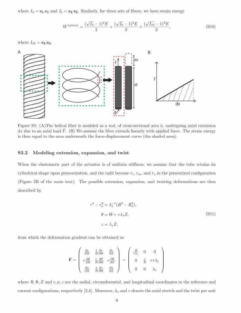
where I4 = s1.s1 and I6 = s2.s2. Similarly, for three sets of fibers, we have strain energy

W (aniso) =(√I4 − 1)2E

2+

(√I6 − 1)2E

2+

(√I10 − 1)2E

2, (S10)

where I10 = s3.s3.

F_

dl

dx

a

BA

dx

F_

ŶŶFigure S5: (A)The helical fiber is modeled as a rod, of cross-sectional area a, undergoing axial extensiondx due to an axial load F . (B) We assume the fiber extends linearly with applied force. The strain energyis then equal to the area underneath the force-displacement curve (the shaded area).

S3.2 Modeling extension, expansion, and twist

When the elastomeric part of the actuator is of uniform stiffness, we assume that the tube retains its

cylindrical shape upon pressurization, and the radii become ri, rm, and ro in the pressurized configuration

(Figure 2B of the main text). The possible extension, expansion, and twisting deformations are then

described by

r2 − r2o = λ−1z (R2 −R2

o),

θ = Θ+ τλzZ,

z = λzZ,

(S11)

from which the deformation gradient can be obtained as

F =

∂r∂R

1R

∂r∂Θ

∂r∂Z

r ∂θ∂R

rR

∂θ∂Θ r ∂θ

∂Z

∂z∂R

1R

∂z∂Θ

∂z∂Z

=

Rrλz

0 0

0 rR

rτλz

0 0 λz

where R,Φ, Z and r, φ, z are the radial, circumferential, and longitudinal coordinates in the reference and

current configurations, respectively [2,4]. Moreover, λz and τ denote the axial stretch and the twist per unit

9

length, respectively. The deformation gradient F is used to calculate the left Cauchy-Green deformation

tensor B = FFT and the current fiber orientation s = FS, from which we obtain the tensor invariants

I1 = tr(B) and I4 = s.s. Finally, we can then use the strain energies of Equations S1 and S2 to calculate

the Cauchy stresses, which take the form

σ(in) = 2W(in)1 B− pI

σ(out) = 2W(out)1 B+ 2W

(out)4 s1 ⊗ s1 + 2W

(out)6 s2 ⊗ s2 − pI

(S12)

where Wi =∂W∂Ii

, I is the identity matrix, and p is a hydrostatic pressure[4].

To determine the current actuator configuration, we first apply the Cauchy equilibrium equations (i.e.

div(σ) = 0), yielding

dσrrdr

=σθθ − σrr

r, (S13)

which can then be integrated to yield

P =

∫ rm

ri

σ(in)θθ − σ

(in)rr

rdr +

∫ ro

rm

σ(out)θθ − σ

(out)rr

rdr, (S14)

where P is the pressure applied inside the tube. Assuming there are no external axial forces or external

axial moments applied to the tube, the axial load N can be obtained as

N = 2π

∫ rm

ri

σ(in)zz rdr + 2π

∫ ro

rm

σ(out)zz rdr = Pπr2i , (S15)

while the axial moment M is given by

M = 2π

∫ rm

ri

σ(in)θz r2dr + 2π

∫ ro

rm

σ(out)θz r2dr = 0. (S16)

10

Equation (S15) can be manipulated as follows:

N = 2π

∫ rm

ri

σ(in)zz rdr + 2π

∫ ro

rm

σ(out)zz rdr

= 2π

∫ rm

ri

(σ(in)zz − σ(in)rr + σ(in)rr )rdr + 2π

∫ ro

rm

(σ(out)zz − σ(out)rr + σ(out)rr )rdr

= 2π

∫ rm

ri

(σ(in)zz − σ(in)rr )rdr + 2π

[

σ(in)rr r2

2

]rm

ri

− 2π

∫ rm

ri

r2

2

dσ(in)rr

dr

+ 2π

∫ ro

rm

(σ(out)zz − σ(out)rr )rdr + 2π

[

σ(out)rr r2

2

]ro

rm

− 2π

∫ ro

rm

r2

2

dσ(out)rr

dr

= 2π

∫ rm

ri

(σ(in)zz − σ(in)rr )rdr + Pπr2i − π

∫ rm

ri

r2σ(in)θθ − σ

(in)rr

rdr

+ 2π

∫ ro

rm

(σ(out)zz − σ(out)rr )rdr − π

∫ ro

rm

r2σ(out)θθ − σ

(out)rr

rdr

= π

∫ rm

ri

(2σ(in)zz − σ(in)rr − σ(in)θθ )rdr + Pπr2i + π

∫ ro

rm

(2σ(out)zz − σ(out)rr − σ(out)θθ )rdr

(S17)

Combining Equations (S15) and (S17), we have

N = π

∫ rm

ri

(2σ(in)zz − σ(in)rr − σ(in)θθ )rdr + Pπr2i + π

∫ ro

rm

(2σ(out)zz − σ(out)rr − σ(out)θθ )rdr = Pπr2i (S18)

Now canceling the Pπr2i on the left side of the equation with the Pπr2i term on the right side of the

equation, we can write the reduced axial load (that is, the axial load due to forces other than the applied

pressure) [3]

Nral = π

∫ rm

ri

(2σ(in)zz − σ(in)rr − σ(in)θθ )rdr + π

∫ ro

rm

(2σ(out)zz − σ(out)rr − σ(out)θθ )rdr = 0. (S19)

Finally, defining λθ =rR

and γ = rτ , and using the identities [2]

σθθ − σrr = λθ∂W

∂λθ+ γ

∂W

∂γ

σθθ + σzz − 2σrr = λθ∂W

∂λθ+ λz

∂W

∂λz

σθz =∂W

∂γ,

(S20)

11

we can write the equilibrium equations in terms of the strain energy:

P =

∫ rm

ri

λz∂W (in)

∂λz+ γ

∂W (in)

∂γ

dr

r+

∫ ro

rm

λz∂W (out)

∂λz+ γ

∂W (out)

∂γ

dr

r(S21)

Nral = π

∫ rm

ri

2λz∂W (in)

∂λz− λθ

∂W (in)

∂λθ− 3γ

∂W (in)

∂γrdr + π

∫ ro

rm

2λz∂W (out)

∂λz− λθ

∂W (out)

∂λθ− 3γ

∂W (out)

∂γrdr = 0

(S22)

M = 2π

∫ rm

ri

∂W (in)

∂γr2dr + 2π

∫ ro

rm

∂W (out)

∂γr2dr = 0 (S23)

Taylor Expansion Since Equations (S21)-(S23) are quite complex and it is computationally intensive

to solve them numerically, for thin-walled actuators we simplify the calculations by Taylor expanding the

equations.

We define ε1 = Rm−Ri

Riand ε2 = Ro−Rm

Rm, and Taylor expand Equations (S21)-(S23). Our goal was to

retain the minimum number of terms required to give an accurate solution. We found that retaining first

order terms in ǫ2 was sufficient, but for ǫ1, we had to retain terms to third order, since ǫ1 ≫ ǫ2. This gave

us the following system of equations:

P =Ri

riλz

∂W1

∂λθε1 +

Rm

rmλz

∂W2

∂λθε2 +

1

2r3i λ2z

[

−R3i

∂W1

∂λθ+ ri(R

2i − r2i λz)

∂2W1

∂λ2θ

]

ε21

+1

6r5iRiλ3z

[

(3R6i − r2iR

4i λz)

∂W1

∂λθ− ri(R

2i − r2i λz)

(

(3R3i + 2r2iRiλz)

∂2W1

∂λ2θ+ ri(−R2

i + r2i λz)∂3W1

∂λ3θ

)]

ε31

+O(ε41) +O(ε22) (S24)

Nral =Riπ

λz

[

2Riλz∂W1

∂λz− ri

∂W1

∂λθ

]

ε1 +Bπ

λz

[

2Rmλz∂W2

∂λz− rm

∂W2

∂λθ

]

ε2

+π

2riλ2z

[

2riR2i λ

2z

∂W1

∂λz−R3

i

∂W1

∂λθ+ (R2

i − r2i λz)

(

2Riλz∂2W1

∂λθ∂λz− ri

∂2W1

∂λ2θ

)]

ε21

+π(−R2

i + r2i λz)

6r3iRiλ3z

[

−R4i

∂W1

∂λθ+ 2R4

i λz∂2W1

∂λθ∂λz+ ri

(

(R3i − 2r2iRiλz)

∂2W1

∂λ2θ− (R2

i − r2i λz)(2Riλz∂3W1

∂λ2θ∂λz− ri

∂3W1

∂λ3θ)

)]

ε31

+O(ε41) +O(ε22) (S25)

M =2riR

2i π

λz

∂W1

∂γε1 +

2rmR2mπ

λz

∂W2

∂γε2 +

Riπ

riλ2z

[

(R3i + r2iRiλz)

∂W1

∂γ+ ri(R

2i − r2i λz)

∂2W1

∂λθ∂γ

]

ε21+

π

3r3iLz3

[

−(R6i − 3r2iR

4i λz)

∂W1

∂γ+ ri(R

2i − r2i λz)

(

R3i

∂2W1

∂λθ∂γ+ ri(R

2i − r2i λz)

∂3W1

∂λ2θ∂γ

)]

ε31

+O(ε41) +O(ε22) (S26)

12

As shown in Figure S6, this expansion is valid for ǫ1 ≤ 0.47 (Figure S6A,B). However, as ǫ1 increases,

the Taylor expansion becomes less accurate. This is shown in Figure S6C, where we have ǫ1 = 0.63, and

observe that the Taylor expansion deviates significantly from the full solution.

pressure (kPa)0 10 20 30 40

λz

1

1.05

1.1

1.15

1.2


τ (°

/mm

)

0

0.5

1

1.5

2


λθ

1

1.5

2

pressure (kPa)0 10 20 30

τ (°

/mm

)

0

0.5

1

1.5

2

pressure (kPa)10 20 30

λz

1

1.05

1.1

1.15

1.2


λθ

1

1.2

1.4

1.6

1.8

2


τ (°

/mm

)

-0.5

0

0.5

1

1.5

2


λz

0.95

1

1.05

1.1

1.15

1.2


λθ

1

1.5

2

2.5

3

A

B

C

Taylor expansionfull solution

α=5°α=25°

α=45°

°

α=65°

°

α=65

α=85°

ε1=0.31, ε

2=1.1 x 10-4

ε1=0.47, ε

2=9.5 x 10-5

ε1=0.63, ε

2=8.6 x 10-6

Figure S6: Comparison of solution using full system of equations (Equations (19)-(21)) with solution usingTaylor expanded equations (Equations (22)-(24)). (A) Results for an actuator with ratios ǫ1 = 0.31 andǫ2 = 1.1 × 10−4. (B) Results for an actuator with ratios ǫ1 = 0.47 and ǫ2 = 9.5 × 10−5. In each of thesecases, we see that the Taylor expansion provides a close approximation to the full solution. However, for athicker-walled actuator, the Taylor expansion becomes less accurate. This is shown in (C), where we haveratios ǫ1 = 0.63 and ǫ2 = 8.6 × 10−6, and observe that the Taylor expansion deviates significantly fromthe full solution.

S3.2.1 Verification of the Model

To verify the analytical model for actuators which extend, expand, and twist, we fabricated some actuators

from Dragon Skin 10 and from Smooth-Sil 950. In Figure S7, we compare the analytical prediction to the

experimental results for two actuators (α = 3◦ and α = 70◦) for each material. Each actuator had inner

13

radius Ri = 6.35mm, wall thickness Ro − Ri = 2mm, and length L = 160mm. The number of fibers was

n = round(13 sinα), and the fibers had radius r = 0.0889mm and Young’s modulus E = 31067MPa. We

found that the response of the actuators was best captured choosing the fitting parameter Ro − Rm =

8.89 × 10−4mm, so that ǫ1 = 0.31 and ǫ2 = 1.1 × 10−4. For this choice of Rm the volume fractions were

c1 =π(R2

o−R2m)L

π(R2o−R2

m)L+n×πr2× Lsinα

and c2 =n×πr2× L

sinα

π(R2o−R2

m)L+n×πr2× Lsinα

. In each case shown in Figure S7, we see good

agreement between the analytical prediction and the experimental results. Some deviations in Figure S7A

are most likely due to inaccuracies in the fabrication procedure. We also see some deviations at higher

pressures in Figure S7B due to the highly nonlinear response of the actuators.


λz

1

1.05

1.1


λθ

1

1.05

1.1

1.15

1.2

1.25

pressure (kPa)0 10 20 30 40 50

λz

1

1.2

1.4

1.6

pressure (kPa)0 10 20 30 40 50

λθ

1

1.2

1.4

1.6

1.8

2

pressure (kPa)0 10 20 30 40 50

τ (

°/m

m)

0

0.5

1

1.5

A Smooth-Sil 950, μ=680kPa:

B Dragon Skin 10, μ=85kPa:


τ (

°/m

m)

0

0.1

0.2

0.3extension expansion twist

extension expansion twistα=3° analyt

α=70° analyt

α=3° exp

α=70° exp

α=3° analyt

α=70° analyt

α=3° exp

α=70° exp

Figure S7: Comparison of experimental results and analytical predictions for (A) Smooth-Sil 950 and (B)Dragon Skin 10. For each material, two actuators are shown: one with fiber angle α = 3◦ and one withfiber angle α = 70◦. Axial stretch λz (left), radial stretch λθ (center), and twist per unit length τ (right)are shown in each case.

We used Finite Element analysis to verify that the model is valid for actuators with different wall

thicknesses (see Figure S8). Each actuator had inner radius Ri = 6.35mm, and length L = 160mm. Wall

thicknesses were either Ro − Ri = 1mm or Ro − Ri = 3mm and materials were either Dragon Skin 10 or

Smooth-Sil 950, as shown in Figure S8. Also in this case we chose Ro − Rm = 8.89 × 10−4mm, so that

ǫ1 = 0.16 and ǫ2 = 1.2 × 10−4 for the thinner actuator and ǫ1 = 0.47 and ǫ2 = 9.5 × 10−5 for the thicker

one. In each case, we see excellent agreement between the analytical predictions and the Finite Element

results.

14

P/µ0 0.1 0.2 0.3

λz

1

1.5

2

P/µ0 0.2 0.4 0.6 0.8

λz

1

1.2

1.4

1.6

1.8

2

P/µ0 0.1 0.2 0.3

λθ

1

1.2

1.4

1.6

1.8

2

P/µ0 0.1 0.2 0.3

τ (°

/mm

)

0

0.5

1

1.5

2A wall thickness 1mm:

B wall thickness 3mm:

P/µ0 0.2 0.4 0.6 0.8

λθ

1

1.5

2

2.5

3

P/µ0 0.2 0.4 0.6 0.8

τ (°

/mm

)

0

0.5

1

1.5

2

α=3° FEM

α=70° FEM

α=3° analyt

α=70° analyt

α=3° FEM

α=70° FEM

α=3° analyt

α=70° analyt

extension expansion twist

extension expansion twist

α

α

Figure S8: Verification of extend/expand/twist model for Dragonskin 10, for wall thicknesses of 1mm and3mm. For each wall thickness, two actuators are shown: one with fiber angle α = 3◦ and one with fiberangle α = 70◦. Axial stretch λz (left), radial stretch λθ (center), and twist per unit length τ (right) areshown in each case.

S3.3 Modeling bending

Since the exact solution for the finite bending of an elastic body is only possible under the assumption

that the cross-sections of the cylinder remain planar upon pressurization - a condition that is severely

violated by our actuator - we assume (i) that the radial expansion can be neglected (i.e. r/R = 1) and (ii)

vanishing stress in the radial direction (i.e. σrr = 0). Furthermore, since the actuators have a symmetric

arrangement of fibers, no twisting takes place, so the deformation gradient reduces to

F =

λz(φ)−1 0 0

0 1 0

0 0 λz(φ)

. (S27)

Since the actuator bends due to the moment created by the internal pressure acting on the actuator caps,

Mcap, the relationship between input pressure and bend angle can be found by equating Mcap to the

opposing moment due to the stress in the material, Mmat.

15

Ri

φ

dh

dφ

dτt1

t2

Figure S9: Cross section of the actuator, with inner radius Ri. The thickness of the inner layer is t1, andtotal wall thickness is t2. The differential angle element is dφ, differential wall thickness element is dτ ,and differential height is dh.

Calculating Mcap To calculate the moment (Mcap) due to air pressure acting on the internal cap of the

actuator, we start by noting that the force due to the air pressure acting on an infinitesimal area of the

actuator cap dA = 2Ri sinφdh is

df = P dA = P 2Ri sinφdh, (S28)

where P is the internal pressure in the actuator, and dφ and dh are the differential angle and height

respectively, as shown in Figure S9. By re-writing h in terms of φ as

h = Ri −Ri cosφ ⇒ dh = Ri sinφdφ, (S29)

we can eliminate h from Equation (S28)

df = P 2R2i sin

2 φdφ. (S30)

The moment acting on the cap is then

Mcap =

∫ 2Ri

0df × distance fromneutral axis

= 2PR2i

∫ π

0sin2 φ abs

[

Ri cos φ−Ri cosφ]

dφ,

(S31)

where φ indicates the position of the neutral axis.

16

Calculating Mmat The moment due to the stress in the material, Mmat, is

Mmat = 2

∫ t1

0

∫ π

π2

λz(φ)−1σ(in,1)zz (Ri + τ)

(

Ri cos φ− (Ri + τ) cosφ)

dφdτ

+ 2

∫ t2

t1

∫ π

π2

λz(φ)−1σ(out,1)zz (Ri + τ)

(


dφdτ

+ 2

∫ t1

0

∫ π2

0λz(φ)

−1σ(in,2)zz (Ri + τ)(


dφdτ

+ 2

∫ t2

t1

∫ π2

0λz(φ)

−1σ(out,2)zz (Ri + τ)(


dφdτ

(S32)

where σ(in,i)zz is the axial stress in the inner isotropic layer with shear modulus µi:

σ(in,i)zz = λ2zµi −µiλ2z

(S33)

and σ(out,i)zz is the axial stress in the outer anisotropic layer with shear modulus µi:

σ(out,i)zz = λ2zµi −µiλ2z

+2√I4

[

(−1 +√

I4)λ2zρ1 sin

2[α]]

+2√I6

[

(−1 +√

I6)λ2zρ2 sin

2[α]]

(S34)

The parameter t1 is the thickness of the inner isotropic layer (Rm − Ri), t2 is the total wall thickness of

the actuator (Ro −Ri), and dτ is the differential thickness of the actuator (Figure S9).

S3.3.1 Obtaining the relationship between input pressure and bend angle

Now solving Mmat =Mcap yields the relationship between input pressure and output bend angle:

P =

t1∫

0

π∫

π2

λ−1z σ

(in,1)zz (Ri + τ)

(


dφ dτ +t2∫

t1

π∫

π2

λ−1z σ

(out,1)zz (Ri + τ)

(


dφ dτ

2R2i

π∫

0

sin2 φabs(

Ri cos φ−Ri cosφ)

dφ

+

t1∫

0

π2∫

0

λ−1z σ

(in,2)zz (Ri + τ)

(


dφ dτ +t2∫

t1

π2∫

0

λ−1z σ

(out,2)zz (Ri + τ)

(


dφ dτ

2R2i

π∫

0

sin2 φabs(

Ri cos φ−Ri cosφ)

dφ

(S35)

S3.3.2 Locating the neutral bending axis

In the bending model, the parameter φ is the circumferential angle where the neutral bending axis is

located. This parameter was determined using an FE simulation for an actuator with fiber angle ±5◦,

17

Ri = 6.35mm, Ro = 8.35mm, and L = 160mm. We found the neutral bending axis occurs at φ = 35◦,

as shown in Figure S10A, where we plot the axial stretch along the line corresponding to φ = 35◦, and

compare it to the maximum axial stretch (which occurs at φ = 180◦). To demonstrate that φ does not

depend on the fiber angle, we also extracted the axial stretch at 35◦ for actuators with fiber angles ±15◦

and ±25◦ (Figure S10B).


λ

1

1.2

1.4

1.6

1.8stretch at φ=35o

stretch at φ=180o

−1.446e−03+4.401e−02+8.946e−02+1.349e−01+1.804e−01+2.258e−01+2.713e−01+3.167e−01+3.622e−01+4.076e−01+4.531e−01+4.985e−01+5.440e−01Rel. radius = 1.0000, Angle = −90.0000

LE, Max. Principal

A B


stre

tch

at φ

=35

°

1

1.2

1.4

1.6

1.8 α1=-α

2=25°

α1=-α

2=15°

α1=-α

2=5°

Figure S10: (A) FEA results for a bending actuator with fiber angle α = ±5◦, at P = 0kPa andP = 40kPa. The material line at φ = 180◦ is highlighted in black, and the line at φ = 35◦ is highlightedin red. The graph shows the corresponding axial stretches. We see that at φ = 35◦, the actuator doesnot change in length. (B) Comparison of axial stretch at φ = 35◦ for bending actuators with fiber anglesα = ±5◦, α = ±15◦ and α = ±25◦. In each case, the stretch is almost unity, showing that we can use theline at φ = 35◦ as the neutral axis.

S3.3.3 Verification of Bending Model

To verify the analytical bending model, we performed FE simulations and compared the results to the

analytical predictions, as shown in Figure S11. In each case (A-D), we used one FE simulation (α = ±5◦)

to find the location of the neutral axis φ. For case A, the thickness of the outer layer, Ro − Rm, was a

fitting parameter found using the extend/expand/twist model. For the other cases, this value was reduced

in proportion to the wall thickness to outer radius ratio (e.g. in case B, the ratio was reduced to 0.66 of

its initial value, so we also reduced the thickness of the outer layer by this amount).

18


ω (

°/m

m)

0

0.5

1

1.5

2

2.5


ω (

°/m

m)

0

1

2

3


ω (

°/m

m)

0

0.5

1

1.5

2

2.5


ω (

°/m

m)

0

0.5

1

1.5

2

2.5


ω (

°/m

m)

0

0.5

1

1.5

2

2.5


ω (

°/m

m)

0

0.5

1

1.5

2

2.5


ω (

°/m

m)

0

0.5

1

1.5

2

2.5


ω (

°/m

m)

0

0.5

1

1.5

2

2.5

effective stiffness:μ_ =104kPa



neutral axis:φ_ =20o





A

B

C

D

α1=-α

2=5° α

1=-α

2=10° α

1=-α

2=15°

α1=-α

2=20° α

1=-α

2=25° α

1=-α

2=30°

FEAanalyt

FEAanalyt

(Rm

-Ri)/R

i=0.079

(Ro-R

m)/R

o=4.3 x 10-5

without e$ective

sti$ness %tting

parameter

with e$ective

sti$ness %tting

parameter (μ_ )

(Rm

-Ri)/R

i=0.118

(Ro-R

m)/R

o=5.5 x 10-5

(Rm

-Ri)/R

i=0.157

(Ro-R

m)/R

o=8.0 x 10-5

(Rm

-Ri)/R

i=0.315

(Ro-R

m)/R

o=1.1 x 10-4

Figure S11: Comparing analytical results to FEA results for various different wall thickness to radiusratios. The column on the left shows results obtained from the model using the experimentally measuredmoduli, while the column on the right shows results obtained using an effective modulus µ (fitted using anFE simulation). As the wall thickness to radius ratio decreases (going from A to D), the analytical modelbecomes much more accurate. In case D, we see that the ratio is small enough that there is no need touse an effective stiffness, as it gives the same results as using the experimentally measured moduli (i.e. forcase D, the graphs in the left and right columns are the same).

When deriving the bending model, we assumed that the actuator walls were thin. As a result, for

thicker walled actuators, the model yields lower than expected bend angles at any given pressure, because

the actuators are too stiff. This can be seen in the left column of Figure S11, which compares analytical

and FE results for actuators with various different ratios of wall thickness to outer radius. We see that as

the thickness to radius ratio decreases, the model gives more accurate results.

In order to use the model for actuators with higher thickness to radius ratios, we use an effective shear

19

modulus in the model, rather than using the experimentally measured moduli. This is illustrated in the

right column of Figure S11. One FE simulation (α = ±5◦) is used to find the effective shear modulus.

Using this fitting parameter (from just one simulation), we can quite accurately predict the deformation

for other fiber angles. As the ratio decreases, we see that there is no need to use this fitting parameter,

since in case D, it gives almost identical results to when the experimentally measured shear moduli are

used.

To experimentally verify the bending model, we fabricated and tested bending actuators with fiber angles

ranging from ±5◦ to ±30◦. The actuators had inner radius Ri = 6.35mm, wall thickness Ro −Ri = 2mm,

and length L = 160mm. Using Rm = 8.89 × 10−4mm and effective shear modulus µ = 78kPa, we found

good agreement between the analytical model and the experimental results (Figure S12).


ω (

°/m

m)

0

1

2

3α

1=-α

2=5°

α1=-α

2=10°

α1=-α

2=15°

α1=-α

2=20°

α1=-α

2=25°

α1=-α

2=30°

analytexp

Figure S12: Comparison of experimental results and analytical predictions of bend angle per unit lengthfor actuators with fiber angles ranging from ±5◦ to ±30◦

S4 Replicating Finger Motion

In this section, we describe the procedure for gathering and processing the data describing the kinematics

of the fingers. We then describe the steps in the optimization algorithm which is used to determine

the optimal design parameters for an actuator which, upon pressurization, will replicate the motion of

the fingers. We use the optimization algorithm to design actuators which replicate the motion of the

index finger and the thumb, and verify the results using finite element analysis. Finally, we outline the

experimental procedure for determining the motion of an actuator in 3d space. Note that the Matlab

scripts corresponding to this section can be found on softroboticstoolkit.com.

S4.1 Processing the input data

We use electromagnetic (EM) trackers to record the coordinates of the index finger and thumb as they

bend. The location of the EM trackers on the hand is illustrated in Figure S13A. The lengths of each of

20

the links and the angles between the links are plotted as a function of time in Figure S14 (index finger)

and Figure S15 (thumb).

= EM tracker

llink,1

( j)Ψ1

Ψ2

θ

llink,2

llink,3

( j)

( j)( j)

( j)

( j)Ψ

3ŶŶ

ŶŶ

ŶŶ

A B

Figure S13: (A) Location of the EM trackers on the index finger and thumb (B) The link lengths llink,iare the lengths between the joints of the finger, while the bend angles ψi are the angles between adjacentlinks, as illustrated above.

time0 50 100 150

leng

th (

mm

)

20

40

60

80

100

50

L1 polynomial fit

L2 polynomial fit

L3 polynomial fit

L4 polynomial fit

4 raw input

50L

1004 polynomial fit

ψ1 polynomial fit

ψ2 polynomial fit

ψ3 polynomial fit

3

4 configurations to match

time0 50 100 150

ψ (

°)

0

20

40

60

80

100link lengths bend angles

Figure S14: Index finger EM tracker data: The dots represent the raw input. This is smoothed using aSavitzky-Golay filter in Matlab, and the smoothed data are plotted as solid lines. Solid squares denotethe four configurations which are selected to be replicated.

21

time0 50 100

θ (

°)

0

20

40

60

80

time0 50 100

leng

th (

mm

)

20

30

40

50

60

4 raw input

50L

1004 polynomial fit

ψ1 polynomial fit

ψ2 polynomial fit

ψ3 polynomial fit

L1 polynomial fit

L2 polynomial fit

L3 polynomial fit

θ polynomial fittime0 50 100

ψ (

°)

0

20

40

60

3

4 configurations to match

twist anglelink lengths bend angles

Figure S15: Thumb EM tracker data: The dots represent the raw input. This is smoothed using aSavitzky-Golay filter in Matlab, and the smoothed data are plotted as solid lines. Solid squares denotethe four configurations which are selected to be replicated.

S4.2 Optimization

We want the optimization to output (1) the fiber angle αi for each segment (2) the initial length l(0)bend,i

of each of the bending segments and (3) the pressures P (j) at which the input configurations will occur

i.e. we want to find the values of the variables αi, l(0)bend,i and P (j) which will achieve the desired link

lengths and bend angles. For the initial values of the variables, we choose pressures equally spaced

between the minimum pressure (0kPa)and maximum pressure (80kPa), and since we want the bend and

twist segment lengths to be as short as possible, we set αi and l(0)bend,i to their minimum allowed values

αi = αmin = 5◦, l(0)bend,i = Lmin = 10mm.

The maximum allowed bend segment length was chosen by doing some preliminary calculations: The

maximum bend angle required for the index finger was 93◦, and the bend angle per unit length for an

actuator with fiber angle 5◦ at the maximum allowed pressure Pmax = 80kPa is 3.3◦/mm. Dividing the

maximum required bend angle by the maximum possible bend per unit length gave a segment length of

28mm. This was rounded up to give a maximum allowed segment length of 30mm.

The main steps in the optimization are as follows:

Step 1

• Given the fiber angle α for each segment and bending and twisting segment lengths, calculate the

initial lengths of the extending segments, as shown in Figure 4 (for example, l(0)ext,2 = l

(0)link,2−

l(0)bend,2

2 −l(0)bend,4

2 ).

• Calculate the extension of the bending segments in each configuration (for example, l(j)bend,2 = l

(0)bend,2+

Riψ(j)2 (cos φ+ 1), where Ri is the inner radius of the actuator.

22

• Use the bend segment lengths in each configuration and the overall link lengths in each configuration

to calculate the required length of each of the extending segments in each configuration (for example,

l(j)ext,2 = l

(j)link,2 −

l(j)bend,2

2 − l(j)bend,4

2 ).

Step 2

• For each extending (or twisting) segment, given the fiber angle αi, use the analytical model to solve

for the segment length l (or twist θ) at each pressure P (j).

• The bending model is an inverse model (given a bend angle, it outputs the pressure at which that

bend angle is achieved). So, for each bending segment, given the fiber angle αi, use the analytical

model to find the pressures P (j) at which the required bend angles ψ are achieved.

Step 3

The function to be minimized is

f = c1

N∑

j=1

ntw∑

i=1

∣

∣

∣θ(j)i − θ

(j)i

∣

∣

∣

2+

N∑

j=1

next∑

i=1

∣

∣

∣l(j)ext,i − l

(j)ext,i

∣

∣

∣

2

+ c2

N∑

j=1

nbend∑

i=1

∣

∣

∣P(j)i − P (j)

∣

∣

∣

2,

(S36)

where ntw, next and nbend are the total number of twisting, extending, and bending segments, respectively,

and N is the number of goal configurations. If f is not sufficiently small, x is updated and the steps are

repeated. When the minimum value of f is found, the fiber angles, segment lengths, and pressures are

output.

S4.3 Glove

In the main text, we used the optimization algorithm to design an actuator where the top of the actuator

mimics the input motion. Here, we use the algorithm to design an actuator where the bottom of the

actuator mimics the input motion. This could be used to design an actuator for use in an assistive glove,

for example [5]. We follow the same procedure as before. The twist and bend angles to be matched are the

same as in the main text, but now the link lengths should be matched by the bottom edge of the actuator.

S4.3.1 Index finger

For the index finger, the optimization determined that the actuator should have extending segments 1,

3, and 6, with lengths 70mm, 21mm, and 16mm respectively, and fiber angles ±33◦, ±15◦, and ±27◦

23

respectively, and bending segments 2, 4, and 5 with lengths 23mm, 28mm, and 15mm respectively, and

fiber angles ±8.1◦, ±5◦, and ±5◦ respectively. We used FEA to investigate the response of an actuator

with this design, and we see in Figure S16 that the FE results are in good agreement with the analytical

prediction.


link

leng

th (

mm

)

20

40

60

80

100


ψ (

°)

0

20

40

60

80

100

l l l lllink,1 Ψ

1Ψ2

llink,2

Ψ3

llink,4

llink,3

-50 0 50 100

0

50

100

150

-50 0 50 100

0

50

100

150 P0

P1

P2

P3

input FEA output

analytical predictionpressure (kPa)60 80

FEA

P=19kPa P=41kPa P=61kPa P=80kPa

A

B

C

link lengths bend angles

finger kinematics

Figure S16: (A) Desired input configurations (left) and achieved FEA output configurations (right) (B)Comparing the input configurations, anaytical prediction, and FEA output for each link length and bendangle (C) FEA results for each of the four configurations

S4.3.2 Thumb

As a second example, we consider the motion of the thumb. This time the optimization determines that the

actuator should have a twisting segment 1 with length 24mm and fiber angle 5◦, extending segments 3, 5,

and 7, with lengths 21mm, 9mm, and 17mm respectively and fiber angles ±8◦, ±5◦, and ±25◦ respectively,

and bending segments 2, 4, and 6, with lengths 14mm, 30mm, and 21mm respectively, each with fiber

24

angle ±5◦. Again, we use FEA to analyze the result, and Figure S17 shows that the FE results and the

analytical prediction match closely.

l l l lθ Ψ1

Ψ2

llink,1

Ψ3

llink,3

llink,2


L (m

m)

20

30

40

50

60


θ (

°)

-20

0

20

40

60

80

pressure (kPa)10 20 30 40 50

ψ (

°)

0

20

40

60

thumb kinematicsanalytical prediction

pressure (kPa)60 80

FEA

-100-50

y0-40

-200

x

0

50

100

20z

-100

y

-50

0-40-20

0

x

20

50

100

0

z

P0

P1

P2

P3

P=5kPa P=36kPa P=50kPa P=55kPa

A

B

C

Ψ3

input FEA output

link lengths bend angles

twist angle

Figure S17: (A) Desired input configurations (left) and achieved FEA output configurations (right) (B)Comparing the input configurations, anaytical prediction, and FEA output for each link length and bendangle, and for the twist angle (C) FEA results for each of the four configurations

S4.4 Thumb actuator: reconstructing 3d motion

Here we describe our procedure for recording the motion of the thumb actuator. Since the thumb actuator

moves out of plane, tracking its motion is slightly more complex than in the case of the finger actuator. In

previous cases, we took a photograph of the actuator at each pressure increment. Now, at each pressure

increment, we take photographs of the actuator from two perspectives, using cameras positioned at right

angles to one another (Figure S18A,C). We post-process the photographs by using Matlab to track the left

25

and right edges of the actuator in each picture. We then find the center line of the actuator by calculating

the average of the left and right sides (Figure S18B,D). Finally, we interpolate the center line, so that the

front view and the side view are sampled at identical z values. We can then combine the x− z data and

the y − z data to find the x− y − z data (Figure S18E).

Y-Z view:

X-Z view:

X-10 0 10 20 30 40

Z

-40

-30

-20

-10

0

40

y

2040

x

200

0

-30

-20

-10

z

X-10 0 10 20 30 40

Z

-40

-30

-20

-10

0

X-10 0 10 20 30 40

Z

-40

-30

-20

-10

0

A

B

C

D

E

Y0 20 40

Z

-40

-30

-20

-10

0

Y0 20 40

Z

-40

-30

-20

-10

0

Y0 20 40

Z

-40

-30

-20

-10

0

40

y

P=0kPaP=19kPaP=22kPaP=28kPaP=31kPaP=34kPaP=40kPaP=43kPaP=52kPaP=56kPa

Figure S18: Reconstructing the motion of segment 6 of the thumb actuator: (A) Front view of the actuatorat 3 different actuation pressures (B) Points on either side of the actuator are tracked in Matlab, and usedto find the center line (C) Side view of the actuator at 3 different actuation pressures (D) Points on eitherside of the actuator are tracked in Matlab, and used to find the center line (E) X-Y and Y -Z values arecombined to find the configurations in X-Y -Z

S5 Video legends

Video S1: A comparison of index finger motion with an actuator designed to replicate this motion.

Video S2: A comparison of thumb motion with an actuator designed to replicate this motion.

26

References

[1] J. E. Adkins and R. S. Rivlin, Large elastic deformations of isotropic materials X. Reinforcement by

inextensible cords, Phil. T Royal Soc A, 248 (1955), pp. 201–223.

[2] F. Kassianidis, Boundary-value problems for transversely isotropic hyperelastic solids, Thesis, Univer-

sity of Glasgow, (2007).

[3] A. Goriely and M. Tabor, Rotation, inversion, and perversion in anisotropic elastic cylindrical tubes

and membranes, Proc Royal Soc A, 469 (2013), pp. 20130011.

[4] R. W. Ogden. Non-Linear Elastic Deformations, Dover, New York, 1984.

[5] P. Polygerinos, Z. Wang, K. C. Galloway, R. J. Wood and C. J. Walsh. Soft Robotic Glove for

Combined Assistance and at-Home Rehabilitation, Robot Auton Syst 73 (2015), pp. 139.

27

Documents

Automatic design of fiber-reinforced soft actuators for trajectory