Embed Size (px)
Citation preview

Automatic Design of Prosodic Features for Sentence
Segmentation
James G Fung
Electrical Engineering and Computer SciencesUniversity of California at Berkeley
Technical Report No. UCB/EECS-2011-140
http://www.eecs.berkeley.edu/Pubs/TechRpts/2011/EECS-2011-140.html
December 16, 2011

Copyright © 2011, by the author(s).All rights reserved.
Permission to make digital or hard copies of all or part of this work forpersonal or classroom use is granted without fee provided that copies arenot made or distributed for profit or commercial advantage and that copiesbear this notice and the full citation on the first page. To copy otherwise, torepublish, to post on servers or to redistribute to lists, requires prior specificpermission.
Automatic Design of Prosodic Features for Sentence Segmentation
by
James G. Fung
A dissertation submitted in partial satisfaction of the
requirements for the degree of
Doctor of Philosophy
in
Electrical Engineering and Computer Science
in the
GRADUATE DIVISION
of the
UNIVERSITY OF CALIFORNIA, BERKELEY
Committee in charge:Professor Nelson Morgan, Chair
Professor Peter BartlettDoctor Dilek Hakkani-TurProfessor Keith Johnson
Fall 2011

The dissertation of James G. Fung is approved:
Co-Chair Date
Date
Date
Co-Chair Date
University of California, Berkeley
Fall 2011

Automatic Design of Prosodic Features for Sentence Segmentation
Copyright 2011
by
James G. Fung

1
Abstract
Automatic Design of Prosodic Features for Sentence Segmentation
by
James G. Fung
Doctor of Philosophy in Electrical Engineering and Computer Science
University of California, Berkeley
Professor Nelson Morgan, Chair
This dissertation proposes a method for the automatic design and extraction of
prosodic features. The system trains a heteroscedastic linear discriminant analy-
sis (HLDA) transform using supervised learning on sentence boundary labels plus
feature selection to create a set of discriminant features for sentence segmentation.
To my knowledge, this is the first attempt to automatically design prosodic features.
The motivation for automatic feature design is to employ machine learning techniques
in aid of a task that hitherto places heavy reliance on time-intensive experimentation
by a researcher with in-domain expertise. Previous prosodic feature sets have tended
to be manually optimized for a particular language, so that, for instance, features de-
veloped for English are comparatively ineffective for Mandarin. While unsurprising,
this suggests that an automatic approach to learning good features for a new lan-
guage may be of assistance. The proposed method is tested in English and Mandarin
to determine whether it can adjust to the idiosyncracies of different languages. This
study finds that, by being able to draw on more contextual information, the HLDA
system can perform about as well as the baseline features.
Professor Nelson MorganDissertation Committee Chair

i
To my parents, Bing and Nancy, who supported me along my path.
To my brother, Steve, for his guidance and inspiration.
To my nieces, Evelyn and Melanie, who are the future.

ii
Contents
List of Figures v
List of Tables viii
1 Introduction 11.1 Feature Design . . . . . . . . . . . . . . . . . . . . . . . . . . . . . . 21.2 Organization . . . . . . . . . . . . . . . . . . . . . . . . . . . . . . . 3
2 Background 52.1 Prosody . . . . . . . . . . . . . . . . . . . . . . . . . . . . . . . . . . 5
2.1.1 Introduction . . . . . . . . . . . . . . . . . . . . . . . . . . . . 52.1.2 Uses of prosody . . . . . . . . . . . . . . . . . . . . . . . . . . 62.1.3 Prosodic features . . . . . . . . . . . . . . . . . . . . . . . . . 9
2.2 Sentence Segmentation . . . . . . . . . . . . . . . . . . . . . . . . . . 122.2.1 Motivation . . . . . . . . . . . . . . . . . . . . . . . . . . . . . 122.2.2 Background . . . . . . . . . . . . . . . . . . . . . . . . . . . . 132.2.3 Evaluation measures . . . . . . . . . . . . . . . . . . . . . . . 162.2.4 Previous work . . . . . . . . . . . . . . . . . . . . . . . . . . . 18
2.3 Feature Selection . . . . . . . . . . . . . . . . . . . . . . . . . . . . . 302.3.1 Filters and ranking . . . . . . . . . . . . . . . . . . . . . . . . 302.3.2 Subset selection methods . . . . . . . . . . . . . . . . . . . . . 322.3.3 Feature construction . . . . . . . . . . . . . . . . . . . . . . . 37
3 Feature Robustness 393.1 Background . . . . . . . . . . . . . . . . . . . . . . . . . . . . . . . . 40
3.1.1 Feature set history and applications . . . . . . . . . . . . . . . 403.2 System . . . . . . . . . . . . . . . . . . . . . . . . . . . . . . . . . . . 48
3.2.1 Classifier . . . . . . . . . . . . . . . . . . . . . . . . . . . . . . 483.2.2 Feature selection . . . . . . . . . . . . . . . . . . . . . . . . . 503.2.3 Corpus . . . . . . . . . . . . . . . . . . . . . . . . . . . . . . . 52
3.3 Results and Analysis . . . . . . . . . . . . . . . . . . . . . . . . . . . 533.3.1 Forward selection results . . . . . . . . . . . . . . . . . . . . . 53

iii
3.3.2 Feature relevancy . . . . . . . . . . . . . . . . . . . . . . . . . 573.3.3 Cross-linguistic analysis . . . . . . . . . . . . . . . . . . . . . 58
3.4 Conclusion . . . . . . . . . . . . . . . . . . . . . . . . . . . . . . . . . 60
4 Feature Extraction with HLDA 614.1 Background . . . . . . . . . . . . . . . . . . . . . . . . . . . . . . . . 62
4.1.1 Linear discriminant analysis . . . . . . . . . . . . . . . . . . . 624.1.2 Heteroscedastic LDA . . . . . . . . . . . . . . . . . . . . . . . 64
4.2 Method . . . . . . . . . . . . . . . . . . . . . . . . . . . . . . . . . . 664.2.1 Motivation . . . . . . . . . . . . . . . . . . . . . . . . . . . . . 664.2.2 System . . . . . . . . . . . . . . . . . . . . . . . . . . . . . . . 674.2.3 HLDA parameters . . . . . . . . . . . . . . . . . . . . . . . . 684.2.4 Feature selection . . . . . . . . . . . . . . . . . . . . . . . . . 734.2.5 Statistical significance . . . . . . . . . . . . . . . . . . . . . . 75
4.3 Results and Analysis . . . . . . . . . . . . . . . . . . . . . . . . . . . 764.3.1 2-word context . . . . . . . . . . . . . . . . . . . . . . . . . . 764.3.2 4-word context . . . . . . . . . . . . . . . . . . . . . . . . . . 794.3.3 Feature selection experiments . . . . . . . . . . . . . . . . . . 824.3.4 Interpretation of HLDA features . . . . . . . . . . . . . . . . . 88
4.4 Conclusion . . . . . . . . . . . . . . . . . . . . . . . . . . . . . . . . . 90
5 Language Independence 945.1 Background . . . . . . . . . . . . . . . . . . . . . . . . . . . . . . . . 95
5.1.1 Tone languages . . . . . . . . . . . . . . . . . . . . . . . . . . 955.1.2 Mandarin lexical tone . . . . . . . . . . . . . . . . . . . . . . . 97
5.2 Method . . . . . . . . . . . . . . . . . . . . . . . . . . . . . . . . . . 1045.3 Results and Analysis . . . . . . . . . . . . . . . . . . . . . . . . . . . 108
5.3.1 Statistical significance . . . . . . . . . . . . . . . . . . . . . . 1085.3.2 2-word context . . . . . . . . . . . . . . . . . . . . . . . . . . 1095.3.3 4-word context . . . . . . . . . . . . . . . . . . . . . . . . . . 111
5.4 Feature Selection . . . . . . . . . . . . . . . . . . . . . . . . . . . . . 1125.5 Feature Analysis . . . . . . . . . . . . . . . . . . . . . . . . . . . . . 1145.6 Conclusion . . . . . . . . . . . . . . . . . . . . . . . . . . . . . . . . . 118
6 Conclusion 122
Bibliography 127
A Pitch Features 146A.1 Basic Variables . . . . . . . . . . . . . . . . . . . . . . . . . . . . . . 146
A.1.1 Pitch statistics . . . . . . . . . . . . . . . . . . . . . . . . . . 146A.1.2 Speaker parameters . . . . . . . . . . . . . . . . . . . . . . . . 147
A.2 Pitch Reset . . . . . . . . . . . . . . . . . . . . . . . . . . . . . . . . 148

iv
A.3 Pitch Range . . . . . . . . . . . . . . . . . . . . . . . . . . . . . . . . 149

v
List of Figures
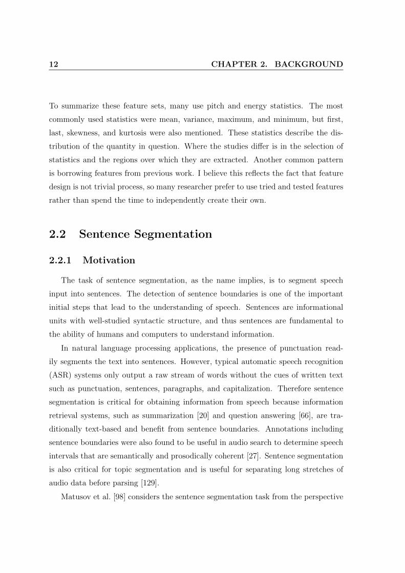
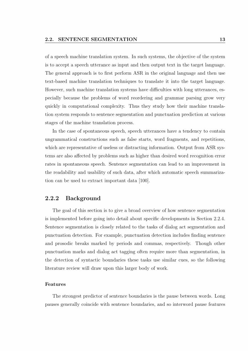
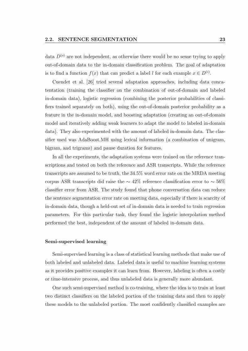
2.1 Components of a factored hidden event language model over wordboundaries Y , words W , and morphological factors M . Solid circlesindicate observations, and dotted circles the hidden events to be in-ferred. The arrows indicate variables used for estimating probabilitiesof boundary Yt, that is P (Yt|Wt,Mt, Yt−1,Wt−1,Mt−1). . . . . . . . . 27
2.2 The search space of a feature selection problem with 4 features. Eachnode is represented by a string of 4 bits where bit i = 1 means theith feature is included and 0 when it is not. Forward selection beginsat the top node and backward elimination begins at the bottom node,with daughter nodes differing in one bit. . . . . . . . . . . . . . . . . 33
2.3 Branch and bound search for selecting a 2-feature subset from 5. Bythe time the algorithm reaches the starred node, it has already searchedleaf node (1,2). If the objective function at the starred node is belowthe bound set by node (1,2), by the monotonicity condition the subtreebelow it cannot exceed the bound and can thus be pruned. . . . . . . 34
3.1 A screenshot of the Algemy feature extraction software. Note the mod-ular blocks used for the graphical programming of prosodic features andhandling of data streams. The center area shows the pitch and energypre-processing steps. . . . . . . . . . . . . . . . . . . . . . . . . . . . 43
3.2 An example of the piecewise linear stylization of a pitch contour, inthis case from Mandarin. The blue dots are the pre-stylization pitchvalues while the green lines show the piecewise linear segments. Thehorizontal axis is in 10ms frames with the purple blocks on the bottomshowing words. Notice that while stylization tends to conform to wordboundaries, the pitch contour for word A has been absorbed by thewords around it and one long linear segment crosses boundary B. . . 45

vi
3.3 An illustration of the performance of feature subsets during forwardselection for Mandarin. The horizontal axis shows F1 score while thevertical gives NIST error rate with the two black lines showing theperformance of the entire prosodic feature set before feature selection.Colors correspond to feature selection iterations: 1 provides the start-ing point, 2 magenta, 3 red, etc. The bold line shows which brancheswere not pruned by the 5th iteration. Note the preference for therightmost branch, which corresponds to the branch with highest F1
score. . . . . . . . . . . . . . . . . . . . . . . . . . . . . . . . . . . . . 55
4.1 The left figure shows the distribution of the two classes if they areprojected along the direction that maximizes the separation of thecentroids. However, because the covariance of the distributions arenot diagonal, the resulting distribution has considerable overlap. Inthe right figure, the data is projected along a direction taking intoconsideration the covariance. While the class means are closer together,there is less overlap and thus less classification error. . . . . . . . . . 64
4.2 Block diagram of the HLDA feature extraction system compared tobaseline system. Both share the same pitch statistics and classifier.Feature selection on HLDA features is optional. . . . . . . . . . . . . 68
4.3 Illustration of 2-word and 4-word context. The input to the HLDAtransform is comprised of the five pitch statistics extracted over eachword in the context, plus the speaker LTM parameter(s). . . . . . . . 70
4.4 Log of the HLDA eigenvalues for English HLDA features from 4-wordcontext and both pitch and log-pitch statistics. Note the sharp drop offat the end occurs in HLDA feature sets using both pitch and log-pitchstatistics due to highly correlated inputs. . . . . . . . . . . . . . . . . 82
4.5 Log of the HLDA eigenvalues for English HLDA features from 4-wordcontext and only log-pitch statistics. Compared to Figure 4.4, there isno sharp drop off at the end. . . . . . . . . . . . . . . . . . . . . . . . 83
4.6 F1 scores on dev and eval sets versus N for Top-N feature setsfrom English 4-word context HLDA features from pitch statistics usingmean fill. dev scores plateau around N=11 while eval continues toslowly increase. An early peak in dev score results in a relatively pooreval score. . . . . . . . . . . . . . . . . . . . . . . . . . . . . . . . . 86
4.7 F1 scores on dev and eval sets versus N for Top-N feature sets fromEnglish 4-word context HLDA features from log-pitch statistics drop-ping missing data. dev scores plateau around N=11 while eval con-tinues to slowly increase. An late peak in dev score results in a rela-tively good eval score. . . . . . . . . . . . . . . . . . . . . . . . . . 86
5.1 Idealized Mandarin lexical tone contours. . . . . . . . . . . . . . . . . 97

vii
5.2 Hypothetical pitch trajectories arguing for the existance of dynamic(sloping) pitch targets rather just high and low static targets from[170]. Figure (a) compares two potential targets, a rising dynamictarget (dotted) and static high target (upper solid line). Starting froma low pitch, because pitch asymptotically approaches targets, the twohypothetical targets would produce the dashed and lower solid line,respectively. Similarly Figure (b) compares a rising dynamic target(dotted) to a sequence of low-high static targets (outer solid lines).Again, these hypothetical targets would produce the dashed and middlesolid line, respectively. The dashed contours are more natural, and soXu concludes the existance of dynamic pitch targets. . . . . . . . . . 101
5.3 Stem-ML tone templates (green) and realized pitch (red). In the firstpair of syllables, the low ending of the 3rd tone and the high start ofthe 4th compromise to a pitch contour between them that also doesnot force the speaker to exert too much effort to change quickly. Thespeaker also manages to hit the template target for the beginning ofthe first syllable and end of the last. In the second pair of syllables, thefirst syllable closely follows the tone template while the second syllableis shifted downward. . . . . . . . . . . . . . . . . . . . . . . . . . . . 102
5.4 The first six principal components from [146]. The 2nd componentlooks like tone 4 and, if negated, resembles tone 2. The 3rd componenthas the falling-rising curve of tone 3. . . . . . . . . . . . . . . . . . . 108
5.5 Distribution of 1st HLDA feature in Mandarin relative to class labeland short vs. long pauses (shorter or longer than 255ms). Takenfrom the 4-word context, log-pitch, drop missing values HLDA featureset. All distributions are normalized to sum to one. Top subplotshows distribution relative to class only while bottom subplot showsdistribution relative to both variables simultaneously. . . . . . . . . . 116
5.6 Distribution of 12th HLDA feature in Mandarin relative to class labeland short vs. long pauses (shorter or longer than 255ms). Takenfrom the 4-word context, log-pitch, drop missing values HLDA featureset. All distributions are normalized to sum to one. Top subplotshows distribution relative to class only while bottom subplot showsdistribution relative to both variables simultaneously. . . . . . . . . . 117
5.7 Distribution of mean pitch of the word immediately before the candi-date boundary in Mandarin relative to class label and short vs. longpauses (shorter or longer than 255ms). All distributions are normal-ized to sum to one. Top subplot shows distribution relative to classonly while bottom subplot shows distribution relative to both variablessimultaneously. . . . . . . . . . . . . . . . . . . . . . . . . . . . . . . 119

viii
List of Tables
2.1 The four possible outcomes for binary classification. . . . . . . . . . . 17
3.1 Corpus size and average sentence length (in words). . . . . . . . . . . 53
3.2 Comparison of performance of prosodic, lexical, and combination sys-tems across all three languages. Recall higher F1 score and lower NISTerror rate are better (see Section 2.2.3). . . . . . . . . . . . . . . . . . 54
3.3 Performance improvement in the three languages over the first seveniterations of the modified forward selection algorithm relative to theperformance of the full feature set. The Type column lists the featuregroup to which each feature belongs using the following code: P =pause; T = speaker turn; F* = pitch (F0); E* = energy; *R = reset;*N = range; *S = slope. Note that repeated listing of FR, ER, etc.refer to different features from within the same feature group, not thesame feature selected repeatedly. . . . . . . . . . . . . . . . . . . . . 56
3.4 Feature groups of the top 15 features that ranked better in the languagenoted than the others. . . . . . . . . . . . . . . . . . . . . . . . . . . 59
3.5 Feature groups of the top 15 features that ranked worse in the languagenoted than the others. . . . . . . . . . . . . . . . . . . . . . . . . . . 60
4.1 Performance of English pitch statistics from 2-word context withoutHLDA transform relative to pause and baseline pitch feature sets. Thethree statistics feature sets are pitch, log-pitch, and their concatenation(both). Eval columns use the posterior threshold trained on the dev
set while oracle uses the threshold that maximizes F1 score on the evalset. . . . . . . . . . . . . . . . . . . . . . . . . . . . . . . . . . . . . . 78
4.2 F1 scores of English HLDA feature sets from 2-word context relativeto the pitch statistics sets they were computed from: pitch, log-pitch,or their concatenation (both). The stat column gives the performanceof the statistics without HLDA. The two HLDA columns indicate themethod of handling missing data. The F1 scores for the pause andbaseline pitch features are provided for comparison. . . . . . . . . . . 78
ix
4.3 Oracle F1 scores of English HLDA feature sets from 2-word contextrelative to the pitch statistics sets they were computed from: pitch,log-pitch, or their concatenation (both). Oracle uses the posteriorthreshold that maximizes the eval F1 score for that feature set. Thestat column gives the performance of the statistics without HLDA. Thetwo HLDA columns indicate the method of handling missing data. Theoracle F1 scores for the pause and baseline pitch features are providedfor comparison. . . . . . . . . . . . . . . . . . . . . . . . . . . . . . . 79
4.4 Performance of English pitch statistics from 4-word context withoutHLDA transform relative to pause and baseline pitch feature sets. Thethree statistics feature sets are pitch, log-pitch, and their concatenation(both). Eval columns use the posterior threshold trained on the dev
set while oracle uses the threshold that maximizes F1 score on the evalset. . . . . . . . . . . . . . . . . . . . . . . . . . . . . . . . . . . . . . 80
4.5 F1 scores of English HLDA feature sets from 4-word context relativeto the pitch statistics sets they were computed from: pitch, log-pitch,or their concatenation (both). The stat column gives the performanceof the statistics without HLDA. The two HLDA columns indicate themethod of handling missing data. The F1 scores for the pause andbaseline pitch features are provided for comparison. . . . . . . . . . . 81
4.6 Oracle F1 scores of English HLDA feature sets from 4-word contextrelative to the pitch statistics sets they were computed from: pitch,log-pitch, or their concatenation (both). Oracle uses the posteriorthreshold that maximizes the eval F1 score for that feature set. Thestat column gives the performance of the statistics without HLDA. Thetwo HLDA columns indicate the method of handling missing data. Theoracle F1 scores for the pause and baseline pitch features are providedfor comparison. . . . . . . . . . . . . . . . . . . . . . . . . . . . . . . 81
4.7 F1 scores of Top-N feature selection experiments for English 2-wordcontext HLDA features. dev-N and oracle-N refer to different stoppingcriteria, where N gives the size of the selected feature set. eval givesthe corresponding F1 score of the eval set. dev-N is based off the dev
set scores while oracle-N chooses the N with maximum eval. . . . . . 84
4.8 F1 scores of Top-N feature selection experiments for English 4-wordcontext HLDA features. dev-N and oracle-N refer to different stoppingcriteria, where N gives the size of the selected feature set. eval givesthe corresponding F1 score of the eval set. dev-N is based off the dev
set scores while oracle-N chooses the N with maximum eval. . . . . . 85

x
4.9 F1 scores of forward selection experiments for English 2-word contextHLDA features. dev-N and oracle-N refer to different stopping crite-ria, where N gives the size of the selected feature set. eval gives thecorresponding F1 score of the eval set. dev-N is based off the dev setscores while oracle-N chooses the N with maximum eval. . . . . . . . 87
4.10 F1 scores of forward selection experiments for English 4-word contextHLDA features. dev-N and oracle-N refer to different stopping crite-ria, where N gives the size of the selected feature set. eval gives thecorresponding F1 score of the eval set. dev-N is based on the dev setscores while oracle-N chooses the N with maximum eval. . . . . . . . 88
4.11 Largest correlations between HLDA feature coefficients. . . . . . . . . 90
5.1 Mean and standard deviation of pitch statistics for Mandarin syllablesby lexical tone. . . . . . . . . . . . . . . . . . . . . . . . . . . . . . . 105
5.2 Mean and standard deviation of pitch statistics for Mandarin syllablesby lexical tone of previous syllable. . . . . . . . . . . . . . . . . . . . 106
5.3 Mean and standard deviation of pitch statistics for English and Man-darin words. . . . . . . . . . . . . . . . . . . . . . . . . . . . . . . . . 106
5.4 Performance of Mandarin pitch statistics from 2-word context withoutHLDA transform relative to pause and baseline pitch feature sets. Thethree statistics feature sets are pitch, log-pitch, and their concatenation(both). Eval columns use the posterior threshold trained on the dev
set while oracle uses the threshold that maximizes F1 score on the evalset. . . . . . . . . . . . . . . . . . . . . . . . . . . . . . . . . . . . . . 110
5.5 F1 scores of Mandarin HLDA feature sets from 2-word context relativeto the pitch statistics sets they were computed from: pitch, log-pitch,or their concatenation (both). The stat column gives the performanceof the statistics without HLDA. The two HLDA columns indicate themethod of handling missing data. The F1 scores for the pause andbaseline pitch features are provided for comparison. . . . . . . . . . . 110
5.6 Oracle F1 scores of Mandarin HLDA feature sets from 2-word contextrelative to the pitch statistics sets they were computed from: pitch, log-pitch, or their concatenation (both). Oracle uses the posterior thresh-old that maximizes the eval F1 score for that feature set. The statcolumn gives the performance of the statistics without HLDA. The twoHLDA columns indicate the method of handling missing data. The or-acle F1 scores for the pause and baseline pitch features are providedfor comparison. . . . . . . . . . . . . . . . . . . . . . . . . . . . . . . 111

xi
5.7 Performance of Mandarin pitch statistics from 4-word context withoutHLDA transform relative to pause and baseline pitch feature sets. Thethree statistics feature sets are pitch, log-pitch, and their concatenation(both). Eval columns use the posterior threshold trained on the dev
set while oracle uses the threshold that maximizes F1 score on the evalset. . . . . . . . . . . . . . . . . . . . . . . . . . . . . . . . . . . . . . 112
5.8 F1 scores of Mandarin HLDA feature sets from 4-word context relativeto the pitch statistics sets they were computed from: pitch, log-pitch,or their concatenation (both). The stat column gives the performanceof the statistics without HLDA. The two HLDA columns indicate themethod of handling missing data. The F1 scores for the pause andbaseline pitch features are provided for comparison. . . . . . . . . . . 112
5.9 Oracle F1 scores of Mandarin HLDA feature sets from 4-word contextrelative to the pitch statistics sets they were computed from: pitch, log-pitch, or their concatenation (both). Oracle uses the posterior thresh-old that maximizes the eval F1 score for that feature set. The statcolumn gives the performance of the statistics without HLDA. The twoHLDA columns indicate the method of handling missing data. The or-acle F1 scores for the pause and baseline pitch features are providedfor comparison. . . . . . . . . . . . . . . . . . . . . . . . . . . . . . . 113
5.10 F1 scores of forward selection experiments for Mandarin 2-word HLDAfeatures. dev-N and oracle-N refer to different stopping criteria, whereN gives the size of the selected feature set. eval gives the F1 score ofthe eval set using the posterior threshold trained on the dev set whileoracle uses the threshold that maximizes F1. dev-N selects N basedoff the dev set scores. oracle-N chooses the N that maximizes eval andoracle individually. . . . . . . . . . . . . . . . . . . . . . . . . . . . . 114
5.11 F1 scores of forward selection experiments for Mandarin 4-word HLDAfeatures. dev-N and oracle-N refer to different stopping criteria, whereN gives the size of the selected feature set. eval gives the F1 score ofthe eval set using the posterior threshold trained on the dev set whileoracle uses the threshold that maximizes F1. dev-N selects N basedoff the dev set scores. oracle-N chooses the N that maximizes eval andoracle individually. . . . . . . . . . . . . . . . . . . . . . . . . . . . . 114
5.12 Frequencies of class labels and short vs. long pauses (shorter or longerthan 255ms) in Mandarin eval set. . . . . . . . . . . . . . . . . . . . 115

xii
Acknowledgments
I would like to thank Dr. Nelson Morgan, whose patient guidance and sage advice
made this dissertation possible. This thesis also owes much to the other members
of the ICSI staff, especially Dr. Dilek Hakkani-Tur and Dr. Elizabeth Shriberg, for
their expertise and support.

1
Chapter 1
Introduction
I begin with two observations:
1. Given sufficient data, statistical learning methods generally outperform systems
dependent on human design.
2. Prosody is complicated, yet prosodic features in speech processing research are
designed by hand.
It seems a bit of an oddity, in a field as permeated by machine learning as speech
processing, that prosodic features are solely designed by a process of researchers
carefully analyzing data, experimenting, and tweaking features. Furthermore, feature
sets are generally designed to work for a specific task, in a particular language, or
under certain conditions, and they can suffer performance degradation because the
assumptions their design was based on have changed.
This dissertation proposes that statistical learning methods can take a bigger
role in feature design. The goal is not to diminish the value of human expertise
or linguistic theory. However, if an automatic system can learn language-specific
behavior, a human researcher does not need to reproduce this work and can instead
focus on other aspects of the problem.

2 CHAPTER 1. INTRODUCTION
1.1 Feature Design
Many machine learning systems achieve success with human-designed features.
Researchers extract features they believe to be useful for the task, and much work
goes into learning algorithms to find exploitable patterns in the features.
This dissertation studies the use of prosody in the task of sentence segmentation,
which is equivalent to finding the location of sentence boundaries. Prosody will be
covered in more detail in Section 2.1, but for now think of it as the pitch, energy,
and duration properties of speech. Prosodic information has found uses in many
speech tasks, including dialog act tagging [5, 33, 139, 165], emotion [4, 143, 171],
segmentation [129, 157, 159], and speaker identity [3, 108, 114].
There are some well-known prosodic cues for breaks between syntactic units:
longer pauses; a slower rate of speech before the boundary; and drop in pitch be-
fore the boundary followed by starting the next unit at a higher pitch, a phenomena
called pitch reset.
Take, for example, the question of how to design feature(s) to capture pitch reset,
as there are other sources of pitch variation besides syntactic unit boundaries. An
upward pitch motion at the end of an utterance generally signals it is a question rather
than a statement. Pitch accents may occur due to stress, which has many uses: it is
what distinguishes the English verb progress and the noun progress ; it occurs from
the metrical pattern of the language; it provides focus within a sentence and can
disambiguate between different interpretations. In tone languages, tones and pitch
accents are part of the lexical identity of words. Furthermore, a speaker’s pattern
pitch patterns can tell the listener about the speaker’s identity and emotional state.
Prosody is complicated, with all manner of information being transmitted through
the manipulation of pitch, energy, and duration. As seen in a review of prosodic
features in Section 2.1.3 and sentence segmentation in Section 2.2.4, many researchers
borrow features from previous work. It is natural for research in the same area to
not reinvent the wheel, but some features are not robust when used in new tasks or
conditions. The design of original features is not trivial; the features in Shriberg [129]
were developed on English data over the course of years, based upon considerable in-
1.2. ORGANIZATION 3
domain knowledge about cues and what features and normalizations would be robust
to unwanted variation. This can be a barrier for researchers wishing to explore a new
domain, language, or task.
Therefore this dissertation sets out to examine how much of this process can be
automated. It does not seek replace human expertise or obviate the need to examine
the data to understand what is going on, but perhaps not all of the feature design
process needs to be done manually.
1.2 Organization
This dissertation is organized as follows: Chapter 2 provides a literature review
and covers background material for the dissertation. In particular, separate sections
are devoted to prosody, sentence segmentation, and feature selection. Section 2.1
covers prosody, its usage in communicating information in speech, and a survey of
prosodic feature sets used in modern speech processing systems. Section 2.2 goes
into detail about the speech processing task of sentence segmentation and the current
state-of-the-art. Section 2.3 gives a survey of various feature selection methods, as
feature selection figures prominently in this work.
Chapter 3 studies the robustness of a set of prosodic features designed by Shriberg
et al. [129] when ported from English to Arabic and Mandarin. As this feature set is
the foundation for the work in the rest of the dissertation, I go into detail about the
features and describe the history and development of the feature set. Feature selec-
tion experiments are used to analyze the robustness of the features. The AdaBoost
classifier used throughout this disseration is also described here.
The lack of robustness in the pitch features to Mandarin lexical tone motivates
the study of automatic feature design. In Chapter 4, I describe the proposed het-
eroscedastic linear discriminant analysis (HLDA) system for the automatic design
and extraction of pitch features. Background for LDA and HLDA are included. The
goal of the chapter is to compare the performance of the proposed system to the
baseline pitch features. The resulting linear transform on input pitch statistics is also
analyzed for any hints to be gleaned for future feature design.

4 CHAPTER 1. INTRODUCTION
Chapter 5 tests the language-robustness of the proposed HLDA system by seeing if
it can compensate for Mandarin lexical tone where the baseline features had trouble.
A survey of tone languages and two leading models of Mandarin lexical tone are
presented for background. Chapter 6 recapitulates the study and presents concluding
remarks.

5
Chapter 2
Background
2.1 Prosody
2.1.1 Introduction
In the study of language, the term prosody has a range of definitions, depending
on the field or where one looks in the literature. On one end of the spectrum are those
who use an abstract definition of prosody that refers to any structure that organizes
sound, including syntactic structure, metrical rhythm, lexical tone and stress, even
the structure of syllables [121]. In this dissertation however, following the tradition of
the speech processing literature, prosody refers to the realization of speech utterances,
including quantities such as pitch intonation, loudness, tempo, and pauses. Machine
learning researchers studying speech often refer to any supersegmental information
not pertaining to lexical identity — words and phones — as prosody, possibly to show
its relationship to the large body of text-based natural language processing research.
These two extreme definitions of prosody share the idea that there exists linguistic
structure that determines, or at least influences, the realization of speech utterances.
The study of prosody in speech processing deals with quantifying these supersegmen-
tal properties and using the observations to infer structure or information about the
utterance. For example, this dissertation studies the use of prosodic information,
especially pitch, for the automatic segmentation of speech into sentence units.

6 CHAPTER 2. BACKGROUND
The quantities associated with prosody include pitch, energy, and duration. It is
the modulation of these properties that speakers use to convey linguistic information
to the listener. While all languages use prosody to communicate, the exact rules for
achieving intended effects vary between languages. This ties into one of the central
questions of this dissertation: How will a machine learning system designed for one
language fare in another, or how much human expertise in one language will transfer
to a different one?
The field of prosody is large but not all of it is relevant to the matter of this
dissertation, such as the psycholinguistics of when and how prosodic information is
used for spoken word recognition [54]. For a review of prosody in the comprehension
of spoken language, see Cutler et al. [28]. In this chapter, Section 2.1.2 illustrates
various examples of prosody. The object is to demonstrate that prosody is used to
transmit a wide range of information, all of which use the same channels: pitch,
energy, and duration. Thus, prosody is the product of many different demands.
Section 2.1.3 gives an overview of prosodic feature sets used to quantify prosody for
various speech processing tasks, which usually try to isolate particular cues from
distracting information in the speech signal.
2.1.2 Uses of prosody
The following give brief summaries of several types of information that prosody is
used to convey.
Syntactic boundaries. Major syntactic boundaries — for instance dialog act and
sentence breaks, or breaks between phrases that might be denoted in text by a comma
— are often marked by pauses, pitch reset, and pre-boundary lengthening, with
stronger events correlating to stronger boundaries. Over the course of a sentence
or phrase, pitch tends to drop to the lower end of the speaker’s range. At the begin-
ning of the next unit, the pitch starts higher. This kind of rapid change occurring at
a boundary is called pitch reset [142]. Pre-boundary lengthening is the tendency for
longer segmental duration and slower rate of speech to precede syntactic boundaries

2.1. PROSODY 7
[162]. Finally, pauses are empirically the strongest cues for breaks between prosodic
units, with long pauses denoting the beginning of a new unit [51].
Resolving ambiguity. There are some word strings that have multiple interpre-
tations. For example, Snedeker and Trueswell [135] studied sentences like, “Tap the
frog with the flower.” For this sentence, the ambiguity lies in whether the flower is a
modifier to the frog or is an instrument with which to tap the frog. In such situations,
prosody is often used to denote which alternative was meant by the speaker. In the
above example, the author noted that different meanings could be detected by word
duration and pauses. Price et al. [110] discusses many situations where prosody aids
disambiguation, including identifying parentheticals and appositions, sentence subor-
dination, and far vs. near and left vs. right attachment.
Utterance position. Prosody can also convey where in the utterance a word occurs.
For example, Grosjean [53] recorded speakers reciting sentences of various lengths.
For example, the sentence “Earlier my sister took a dip” can be extended another
three, six, or nine words with the phrases “... in the pool / at the club / on the hill.”
When played each recording up to word “dip,” listeners could often differentiate how
many more words the utterance contained. Oller [106] studied the differences in seg-
mental duration in the initial, medial, and final positions of utterances, including
pre-boundary lengthening mentioned above.
Speaker identity. While some might not include speaker identity as part of prosody
because it is a property of the speaker, not what is being said, speakers can be rec-
ognized by their distinctive usage of the components of prosody. Pitch and energy
distributions and dynamics have also helped differentiate speakers [3]. Furthermore,
every speaker has an idiolect, with their personal patterns of word choice and pro-
nunciation [23].
Emotion. The speaker’s emotional state can also surface in their prosody. For ex-
ample, activity or arousal correlate with increased pitch height, pitch range, energy,

8 CHAPTER 2. BACKGROUND
rate of speech. In contrast, anger often exhibits a flat pitch contour with occasional
spikes in pitch and energy. For a review of the use of prosody in communicating
emotion, see Frick [39].
Lexical stress. While the speech processing literature generally excludes lexical
information from the definition of prosody, it is important to note that the compo-
nents of prosody can be used to convey lexical information as well. In English, moving
word stress can change a verb into a noun, which are called initial-stress-derived nouns
[61], such as conduct and permit. The realization of word stress varies from language
to language and may include pitch accents, pitch excursions, or accents marked by
changes in loudness or segmental duration. Stressed syllables tend to better enun-
ciated than unstressed syllables and hence more easily recognized [88]. Kochanski
et al. [77] showed that even tone languages may follow this pattern, where speakers
follow the tone template more closely in syllables with greater prosodic weight than
in weaker syllables.
Lexical tone and pitch accent. Tone languages use pitch to distinguish words,
the common example probably being the word “ma” in Mandarin, which may mean
mother, hemp, horse, or to scold, depending on whether tone 1 through 4 is used,
respectively. I cover tone languages in more depth in Section 5.1.1.
All of the above are communicated through the modulation of the same pitch, en-
ergy, and duration characteristics of speech. Separating relevant information from
distractions is thus non-trivial. Indeed, as we shall see in Chapter 3, Mandarin lex-
ical tones are conflated with the sentence pitch contour. As a result, pitch features
from Shriberg et al. [129] that work well for sentence segmentation in English and
Arabic do not perform as well in Mandarin.

2.1. PROSODY 9
2.1.3 Prosodic features
The objective of the following is to give an overview of the sorts of prosodic fea-
tures used in modern speech processing systems.
Sentence/Dialog act segmentation. One feature set [129] designed by Shriberg,
which the work in this dissertation is based on, is detailed in Section 3.1. To summa-
rize, it contains pause, pitch, energy, and duration features. Pause duration is a strong
predictor for unit boundaries. The pitch features are based on word-level statistics of
the pitch contour and aim to detect pitch reset. The duration features describe rate
of speech and segmental duration, in particular the last vowel and rhyme before the
candidate boundary. This feature set grew out of work on disfluency detection and
speaker verification, has been employed in the segmentation of sentences, dialog acts,
and topics, and has also found usage in emotion-related tasks, among others.
Warnke et al. [159] also concentrated on the word-final syllable, using duration,
pause, pitch contour, and energy quantities over six syllables as the input to a multi-
layer perceptron (MLP). This was combined with various N -gram language models
(LM). A later study by Wang et al. [157] attempted speech segmentation without us-
ing automatic speech recognizer (ASR) output included in many feature sets. They
used a vowel/consonant/pause classifier based on energy. Sufficiently long pauses are
candidate boundaries. Using vowels to locate syllables, they calcuated short-term
rate of speech features. Pitch features are also calculated looking at the six sylla-
bles surrounding the candidate boundary, looking for pitch reset and syllable contour
shape.
Dialog act tagging. Interestingly, the prosodic features used in dialog act tag-
ging and segmentation have much in common, possibly because many researchers
work in these closely related tasks. For example, the Warnke [159] paper discussed
above also classified the dialog acts it identified, though this classification mainly
relied on their LMs. Both Ang et al. [5] and Stolcke et al. [139] used the Shriberg
feature set described in [129], though [139] focused on discourse grammar, an N -gram

10 CHAPTER 2. BACKGROUND
model of dialogue act sequencing in conversation, and lexical data.
To give an idea of dialog act tagging prosodic feature sets not borrowed from
segmentation systems, Fernandez and Picard [33] took the pitch and energy contours
and their first two derivatives and extracted a variety of statistics, including variance,
skewness, and kurtosis. They also included a duration feature measuring the length
of the voiced speech. Wright et al. [165] used similar pitch, energy, and duration
features, adding pitch features from regions of interest within the utterance. For ex-
ample, they identified accents [144] and extracted starting pitch, amplitude, duration,
and shape of the accent. They also extracted pitch and energy features over the last
400ms of the utterance, and their analysis of feature usage found that features from
the tail of the utterance and the last accent were particularly useful.
Speaker identification. As opposed to many speech processing tasks where it
is desirable to normalize out variation due to speakers, speaker identification / recog-
nition / verification seeks to do the reverse. Bimbot et al. [13] advocate the use of
linear predictive coding (LPC)-based cepstral acoustic features plus delta and double
delta cepstral parameters as well as delta energy parameters. Pre-emphasis is per-
formed to enhance high frequencies, cepstral mean subtraction helps remove slowly
varying convolutive noise, and frames of silence and background noise are removed to
leave only speech. Because LPC cepstral coefficients reflect short-term information,
care must be taken that the speaker model captures speaker characteristics instead
of what is being said.
Reynolds et al. [114] combined the work of several sites. Their final system used
short-term acoustic cepstral-based features like the above from Reynolds et al. [115].
From Adami et al. [3], they used frame-based log-pitch and log-energy distributions
and pitch and energy gestures. These gestures are composed of sequences of pitch
and energy slope states combined with segmental duration and phone or word con-
texts, so that is not a purely prosodic model. The system also used some duration
and pitch statistics extracted over word-sized windows from Peskin et al. [108]. The
combined model also made use of some phone and lexical features, among which the
pronunciation modeling made the most significant contribution.

2.1. PROSODY 11
Emotion detection. To detect annoyance and frustration, say when a user finds
an automated call system not helpful, Ang et al. [4] borrowed many features from
the aforementioned Shriberg prosody features [129]. The duration/rate of speech and
pause features are identical. The pitch and energy features used the same prepro-
cessing, but the features were mainly interested in peaks, such as the maximum value
over the utterance or inside the longest normalized vowel. Spectral tilt features, which
measure the distribution of energy in the frequency spectrum, were also computed on
the longest normalized vowel. Lexical information came in the form of word trigrams.
The study found slower rate of speech and sharper pitch contours to be indicative of
frustration.
In contrast, Tato et al. [143] and Yacoub et al. [171] attempted multi-class classifi-
cation with labels ’angry,’ ’bored,’ ’happy’, ’sad,’ and ’neutral.’ For prosodic features,
both used statistics of the pitch contour, its derivative, and jitter; this last highlights
frequency changes in the signal. The statistics were selected to describe the distri-
bution of the variable: minimum, maximum, mean, standard deviation, etc. Corre-
sponding energy features were calculated in the same manner on the energy contour,
its derivative, and shimmer/tremor, the energy analog of jitter. Both also extracted
duration features, looking for patterns in the energetic segments of the utterance,
such as their length or what proportion of the utterance was energetic. Tato used
voiced vs. unvoiced frames while Yacoub split loud vs. quiet frames by thresholding
energy. Tato also used voice quality features related to articulatory precision and
vocal tract properties. These included formant bandwidth, harmonic to noise ratio,
voiced to unvoiced energy ratio, and glottal flow.
Tato found that the pitch and energy features were useful in differentiating be-
tween high, low, and neutral levels of arousal while the quality features helped decide
between emotions once the arousal level was known. In distinguishing hot anger from
neutral utterances, Yacoub found the most useful features were based on the deriva-
tive of the pitch contour, jitter, and maximum energy. When distinguishing between
hot/cold anger and neutral/sadness, the best features instead were pitch, jitter, au-
dible duration, and maximum energy.
12 CHAPTER 2. BACKGROUND
To summarize these feature sets, many use pitch and energy statistics. The most
commonly used statistics were mean, variance, maximum, and minimum, but first,
last, skewness, and kurtosis were also mentioned. These statistics describe the dis-
tribution of the quantity in question. Where the studies differ is in the selection of
statistics and the regions over which they are extracted. Another common pattern
is borrowing features from previous work. I believe this reflects the fact that feature
design is not trivial process, so many researcher prefer to use tried and tested features
rather than spend the time to independently create their own.
2.2 Sentence Segmentation
2.2.1 Motivation
The task of sentence segmentation, as the name implies, is to segment speech
input into sentences. The detection of sentence boundaries is one of the important
initial steps that lead to the understanding of speech. Sentences are informational
units with well-studied syntactic structure, and thus sentences are fundamental to
the ability of humans and computers to understand information.
In natural language processing applications, the presence of punctuation read-
ily segments the text into sentences. However, typical automatic speech recognition
(ASR) systems only output a raw stream of words without the cues of written text
such as punctuation, sentences, paragraphs, and capitalization. Therefore sentence
segmentation is critical for obtaining information from speech because information
retrieval systems, such as summarization [20] and question answering [66], are tra-
ditionally text-based and benefit from sentence boundaries. Annotations including
sentence boundaries were also found to be useful in audio search to determine speech
intervals that are semantically and prosodically coherent [27]. Sentence segmentation
is also critical for topic segmentation and is useful for separating long stretches of
audio data before parsing [129].
Matusov et al. [98] considers the sentence segmentation task from the perspective
2.2. SENTENCE SEGMENTATION 13
of a speech machine translation system. In such systems, the objective of the system
is to accept a speech utterance as input and then output text in the target language.
The general approach is to first perform ASR in the original language and then use
text-based machine translation techniques to translate it into the target language.
However, such machine translation systems have difficulties with long utterances, es-
pecially because the problems of word reordering and grammar parsing grow very
quickly in computational complexity. Thus they study how their machine transla-
tion system responds to sentence segmentation and punctuation prediction at various
stages of the machine translation process.
In the case of spontaneous speech, speech utterances have a tendency to contain
ungrammatical constructions such as false starts, word fragments, and repetitions,
which are representative of useless or distracting information. Output from ASR sys-
tems are also affected by problems such as higher than desired word recognition error
rates in spontaneous speech. Sentence segmentation can lead to an improvement in
the readability and usability of such data, after which automatic speech summariza-
tion can be used to extract important data [100].
2.2.2 Background
The goal of this section is to give a broad overview of how sentence segmentation
is implemented before going into detail about specific developments in Section 2.2.4.
Sentence segmentation is closely related to the tasks of dialog act segmentation and
punctuation detection. For example, punctuation detection includes finding sentence
and prosodic breaks marked by periods and commas, respectively. Though other
punctuation marks and dialog act tagging often require more than segmentation, in
the detection of syntactic boundaries these tasks use similar cues, so the following
literature review will draw upon this larger body of work.
Features
The strongest predictor of sentence boundaries is the pause between words. Long
pauses generally coincide with sentence boundaries, and so interword pause features

14 CHAPTER 2. BACKGROUND
are used in virtually every sentence segmentation system. The main source of confu-
sion with pause features comes, of course, when the speaker pauses in the middle of
a sentence, such as when taking a breath or deciding how to finish the sentence [140].
This leads to oversegmentation, and the usual way to address these classifier errors
is to use additional information sources. The two most common such information
sources are prosodic information and language models.
Prosodic features. Prosody was discussed in Section 2.1. In comparison to purely
text-based methods, speech provides prosodic information through its durational, in-
tonational, and energy characteristics. In addition to its relevance to discourse struc-
ture in spontaneous speech and its ability to contribute to various tasks related to
the extraction of information, prosodic cues are generally unaffected by word identity.
Prosodic information has been found to complement lexical data from ASR output
and thus improve the robustness of information extraction methods that are based on
ASR transcripts [57, 59, 129]. A sample of prosodic feature sets was given in Section
2.1.3 and the prosodic features used by this work are detailed in 3.1.
Language models. The purpose of a language model is to predict the probabil-
ity of any particular word in a given situation. For example, a unigram language
model considers each word independently. For any given English word, one would far
more likely expect “the” or similar function words than “Galapagos.” A commonly
used language model is the N -gram language model, which assumes word strings fol-
low the Markov property and estimates the probability of a word from the contextual
history of the previous N−1 words. That is the probability of a sequence of m words
is estimated by:
P (w1, . . . , wm) =m∏i=1
P (wi|w1, . . . , wi−1)
≈m∏i=1
P (wi|wi−(N−1), . . . , wi−1)
To continue our example, following the word “Galapagos,” a language model may
expect “Islands” more than the far more common word “the.” Thus language models

2.2. SENTENCE SEGMENTATION 15
are used to decide what words make sense together and in particular contexts.
More complicated language models can take into consideration other features of
words, including their parts of speech or position in a sentence. Due to the very large
vocabularies used in many tasks, common issues in language models include dealing
with words not present in its training set and data fragmentation, i.e. for an N -gram,
not all N − 1 sequences of words will occur in even a very large training set, so there
is very little data to train models for each context. For further discussion of language
models, see [70, 97].
Classifers
Usually the simplest method of sentence segmentation from a stream of speech is
through the use of word-boundaries, in which case the task becomes a classification
problem: each word-final boundary is classified as the end of the sentence or not. Sen-
tences can be further classified based on the type of sentence, for example declarative,
interrogative, unfinished, etc. by dialog act tagging. I will treat sentence segmenta-
tion as binary classification of word-final boundaries into non-sentence boundaries (n)
and sentence boundaries (s).
A common technique used with prosodic information is to make the simplifying
assumption of a bag-of-words model, that the words (and boundaries) are unordered
and conditionally independent given their observations. Then a classifier is trained
to estimate the posterior probability P (bi = s|oi), where bi is the ith boundary and
oi are its associated observations. A word-final boundary is then classified as a sen-
tence boundary if the posterior probability exceeds a chosen threshold. Obviously the
boundary decisions should not be independent — in conditions where short sentences
are rare, the presence of a sentence boundary should reduce the likelihood of another
boundary in the vicinity — but the idea is for the observations oi to incorporate
relevant contextual information from surrounding words in order to simplify the clas-
sifier. For these bag-of-words models, discriminative models such as classification and
regression tree (CART) decision trees and support vector machine (SVM) classifiers
have been used.

16 CHAPTER 2. BACKGROUND
In contrast, lexical information in the form of N -gram LMs typically use a gen-
erative sequence model that makes use of the word sequence, such as hidden Markov
models (HMM). For the purposes of sentence segmentation and punctuation pre-
diction, sentence boundaries and punctuation may be treated as tokens in the word
stream or as properties of words, such as in hidden event models. In this way, language
models can utilize patterns about the placement of sentence breaks and punctuation in
the data. For example, “The” commonly appears at the beginning of sentences while
punctuation usually does not occur in the middle of “Queen Victoria.” The following
example from [51] shows one way lexical information can cue sentence boundaries
(indicated in the following by a semi-colon):
... million pounds a year in the UK; and worldwide it’s an industry worthseveral billion; but it’s thought...
They noted that sentence structure in broadcast news speech differs from that of
written language, and some words such as “and” and “but” often appeared at the
beginning of new sentences. Therefore a language model trained on this data would
give higher likelihoods to word strings with sentence boundaries before such words
than not.
2.2.3 Evaluation measures
Before going forward, it will be useful to discuss the performance measures used
in the experiments in this thesis. As a binary classification problem, each example
falls into one of four categories, as seen in Table 2.1. Let S = Ss + Sn be the number
of true sentence boundaries, where Sn is the number of true boundaries misclassified
as non-boundaries, i.e. false negative errors. Similarly, there are Ns false positive
errors, true non-sentence boundaries wrongly labeled as sentence boundaries.
Precision denotes the fraction of sentence boundary labels that are correct:
p =Ss
Ss +Ns
To achieve high precision, a classifier could return the single sentence boundary it is
more confident of. Lower precision indicates the sentence boundary labels are less
likely to be correct.

2.2. SENTENCE SEGMENTATION 17
TruthNon-sentence Sentence
ClassifierNon-sentence
Nn SnTrue negative False negative
SentenceNs Ss
False positive True positive
Table 2.1: The four possible outcomes for binary classification.
Recall describes what percentage of the reference sentence boundary were found:
r =SsS
=Ss
Ss + Sn
To achieve high recall, the classifier could label all boundaries as sentence boundaries.
Lower recall means the classifier failed to find all of the reference sentence boundaries.
NIST error rate is a measure commonly used in evaluations, starting with those
organized by the National Institute of Standards and Technology [160]. It is defined
as the average number of misclassifications per actual sentence boundary:
NIST error rate =Sn +Ns
S
In the case of sentence segmentation, this can exceed 100%. There are far more non-
sentence boundaries than sentence boundaries, so any trigger-happy classifier may
have high recall but insert sentence breaks where none exist.
As can be seen, precision and recall are designed to be in opposition, precision
penalizing an overly-zealous classifier making false positive errors and recall penalizing
a conservative classifier making false negative errors. The only way to score 100%
in both precision and recall is to classify all boundaries correctly. Fβ is a measure
devised to capture both precision and recall when the user weights recall β times
more than precision [153]:
Fβ = (1 + β2)pr
β2p+ r(2.1)
The most common version used is β = 1, also known as F1 score or simply F -score
or F -measure. For F1 score, (2.1) simplifies to the harmonic mean of precision and

18 CHAPTER 2. BACKGROUND
recall:
F =2pr
p+ r
=1
1/p+ 1/r
To give an intuition of what this means, take two numbers a and b, and let a > b.
Then a ≥ their arithmetic mean ≥ their geometric mean ≥ their harmonic mean ≥ b.
That is the harmonic mean will be closer to the lower of the two values. Thus, under
F1 score, neither precision nor recall can be ignored. In the following experiments,
we will find that F1 score tends to be a more reliable measure for system performance
than NIST error.
2.2.4 Previous work
Model combination
Hakkani-Tur et al. [59] used both prosodic features and language models for sen-
tence and topic segmentation. The prosodic features used were an early version of
Shriberg [129] using CART-style decision trees to predict the boundary type. Due
to the greedy nature of decision trees, smaller subsets of features can produce better
results than the initial larger feature set. In order to improve computational efficiency
and remove redundant features, an iterative feature selection algorithm was used to
locate subsets of useful task-specific features.
The training of the prosodic model was done on a training set of 700,000 words.
In comparison, the HMM using an N -gram language model was trained on the same
training set and also on a far larger 130 million word dataset, almost a 200-fold
increase in training data. Due to data fragmentation, N -gram language models may
greatly benefit from additional training data. This also reflects the relative availability
of text data versus annotated speech data. The prosodic model outperformed all the
language models save one, though the prosodic model had access to interword pause
duration features while the language models did not. The language model exception
was trained on the larger 130 million word data set and incorporated speaker turn

2.2. SENTENCE SEGMENTATION 19
boundaries as pseudo-words, since a speaker ceasing to speak is a good indicator of
their having completed a sentence.
The classification problem is to find the optimal string of classifications T for:
argmaxT
P (T |W,F )
where F is the sequence of prosodic features and W is the string of words. The
prosodic and lexical information were combined by using the posterior probabilities
of the prosodic feature decision trees as emissions from the HMM system as likelihoods
P (Fi|Ti). To convert the posterior probabilities P (Ti|Fi) to likelihoods, they chose
to train the decision trees on a resampled version of the training set with a balanced
number of sentence and non-sentence boundaries, which allowed them to avoid having
to calculate prior probabilities:
P (Ti|Fi) =P (Fi|Ti)P (Ti)
P (Fi)
∝P (Fi|Ti)P (Ti)
∝P (Fi|Ti)
using the fact that P (Fi) is constant for Ti and P (Ti) is constant because of the
resampling.
The prosodic feature decision achieved 4.3% classification error rate, the best
language model HMM scored 4.0% error rate, and the combination of the two infor-
mation sources produced a 3.2% classification error rate. Note that the chance error
rate for this broadcast news domain corpus is 6.1% achievable by always guessing
non-sentence labels.
Gotoh and Renals [51] approached the problem by noting that conventional ASR
systems use language models that include sentence markers and are thus able to do
some sentence segmentation. However, because the emphasis in large vocabulary
speech recognition is on the sequence of words rather than the overall structure, the
performance is unsatisfactory, with about 60% precision and recall for the broadcast

20 CHAPTER 2. BACKGROUND
news corpus they used. Thus they sought to identify sentence breaks from the ASR
transcripts, which included sentence and silence markers that were very likely to be
sentence breaks. They noted that the reference transcripts used for training were
not exactly truth as they came from scripts prepared before the broadcast; they were
quite close but might have had a slight negative impact on their results.
Their baseline system was a bigram finite state language model, with each state
composed of a word and sentence boundary class pair and conditioned on the pre-
vious state. To this they added a pause duration model, estimating the probability
of sentence break given the length of the pause to the nearest 0.1s. Because of the
added complexity of having a bigram finite state model with states composed of
sentence boundary class, word, and pause feature, they tried a couple of model de-
compositions, making simplifying assumptions about the independence of variables
and between adjacent states, resulting in models that more closely resemble familiar
HMMs with their hidden states and observed emissions. The study found their pause
duration model, language model, and their combination produced 46%, 65%, and
70% F1 score, respectively.
Shriberg et al. [129] used both prosodic and language modeling in their study.
Prosodic modeling was used to extract features and language modeling to capture
information about sentence boundaries and to model the joint distribution of bound-
ary types in an HMM. The study compared several methods for combining the two
models:
• Posterior probability interpolation: A linear interpolation between the posterior
probabilities of the language model HMM and prosodic decision tree.
• Integrated hidden Markov modeling: An extension of Hakkani-Tur et al. [59],
the prosodic observations are treated like emissions of the HMM used for lexical
modeling. A model combination weight parameter was added to trade-off the
contributions of the language model and prosodic information.

2.2. SENTENCE SEGMENTATION 21
• HMM posteriors as decision tree features: The posterior probability of the lex-
ical model HMM is used as a feature in the prosody decision tree. However,
the authors found that the decision trees had an overreliance on the posteriors
from the HMM, which was trained on correct words, while the test data was
ASR outputs.
The paper argues that the main strength of HMMs, as likelihood models that
describe observations given hidden variables, is that they can integrate local evidence,
such as lexical and prosodic observations, with models of context, i.e. the sequence of
boundary events, in a computationally efficient way. However, they make assumptions
regarding the independence of observations and events which may not be entirely
correct and thus limit performance.
In comparison a posterior model, such as the prosodic decision tree, tries to model
the probability of the hidden variables as a function of the observations. The benefit
is that model training is directed to improving discrimination between target classes
and different features can generally be combined easily. The downside is that such
classifiers can be sensitive to skewed class distributions, classification with more than
two target classes complicates the problem because of the interaction of decision
boundaries, and discrete features with large ranges — e.g. word N -grams — are not
easily handled by most posterior models.
The results showed that prosodic information alone performs comparably to lexical
information, and that their combination leads to further improvement. One interest-
ing observation was that the integrated HMM performed better on reference output
while interpolated posteriors were more robust to ASR output errors.
Mrozinski et al. [100] adapted the sentence segmentation model from Stolcke and
Shriberg [140], which accounts for sentence boundaries truncating the word history
in the training data. A hidden segment model hypothesizes the presence or absence
of a segment boundary between each two words. Thus each word has two states,
corresponding to whether a segment starts before the word or not, and likelihood

22 CHAPTER 2. BACKGROUND
models for each state must be derived from the traditional N -gram model to take
into account truncated histories due to sentence boundary states. In this way, the
model implicitly computes the likelihood of all possible segmentations. With this,
[100] combined three separate language models, two using word-based language mod-
els and a class-based language model from [102]. No prosodic features were used in
this system.
Adaptation
Supervised learning requires that the training corpus be labeled. Manual labeling
of data is a very costly and time consuming task while automatic labeling may intro-
duce errors, which may have repercussions for learning algorithms trained upon it.
Adaptation is a method that circumvents this problem by using out-of-domain data
that has already been labeled or cleaned to build or improve a classification model
for in-domain data. Like supervised and unsupervised learning, there is supervised
and unsupervised adaptation, depending on whether some of the in-domain data is
already labeled.
Cuendet et al. state in [26] that theirs is the first published attempt to apply adap-
tation to sentence segmentation. The paper describes the supervised adaptation of
conversation telephone speech (CTS), in this case Switchboard data, to meeting-style
conversations. The benefits of using CTS include the large amounts of labeled data
and the conversational speaking style that it shares with meeting data. As opposed
to broadcast news, CTS and meeting conversations include speech irregularities such
as disruptions and floor-grabbers/holders. The primary differences between CTS and
meetings are that meetings generally have more than two speakers and the speakers
also use visual contact to communicate.
The underlying assumption in adaptation is that, for each example xi, there exists
a probability distribution p(xi, lj) for each possible label lj. Furthermore, the proba-
bility distributions p(i)(xi, lj) for in-domain data D(i) and p(o)(xi, lj) for out-of-domain
2.2. SENTENCE SEGMENTATION 23
data D(o) are not independent, as otherwise there would be no sense trying to apply
out-of-domain data to the in-domain classification problem. The goal of adaptation
is to find a function f(x) that can predict a label l for each example x ∈ D(i).
Cuendet et al. [26] tried several adaptation approaches, including data conca-
tentation (training the classifier on the combination of out-of-domain and labeled
in-domain data), logistic regression (combining the posterior probabilities of classi-
fiers trained separately on both), using the out-of-domain posterior probability as a
feature in the in-domain model, and boosting adaptation (creating an out-of-domain
model and iteratively adding weak learners to adapt the model to labeled in-domain
data). They also experimented with the amount of labeled in-domain data. The clas-
sifier used was AdaBoost.MH using lexical information (a combination of unigram,
bigram, and trigrams) and pause duration for features.
In all the experiments, the adaptation systems were trained on the reference tran-
scriptions and tested on both the reference and ASR transcripts. While the reference
transcripts are assumed to be truth, the 34.5% word error rate on the MRDA meeting
corpus ASR transcripts did raise the ∼ 42% reference classification error to ∼ 56%
classifier error from ASR. The study found that phone conversation data can reduce
the sentence segmentation error rate on meeting data, especially if there is scarcity of
in-domain data, though a held-out set of in-domain data is needed to train regression
parameters. For this particular task, they found the logistic interpolation method
performed the best, independent of the amount of labeled in-domain data.
Semi-supervised learning
Semi-supervised learning is a class of statistical learning methods that make use of
both labeled and unlabeled data. Labeled data is useful to machine learning systems
as it provides positive examples it can learn from. However, labeling is often a costly
or time-intensive process, and thus unlabeled data is generally more abundant.
One such semi-supervised method is co-training, where the idea is to train at least
two distinct classifiers on the labeled portion of the training data and then to apply
these models to the unlabeled portion. The most confidently classified examples are

24 CHAPTER 2. BACKGROUND
then added to the labeled training data, and this process can be iterated to grow the
amount of labeled training data without too much loss in accuracy.
Guz et al. [57] applied co-training to sentence segmentation using classifiers trained
on lexical and prosodic information, which provide separate and completary views of
the sentence segmentation task. Both classifiers used a boosting algorithm (BoosT-
exter). The prosodic information classifier used 34 features, including pause duration
and pitch and energy features. The lexical classifier used 6 N -gram features no longer
than trigrams.
The exact co-training algorithms used were extensions of the one used in [158].
In general, one could view co-training as a method for improving the training set for
a supervised learning classifier. However, in the case of co-training, the training set
for each classifier can be adjusted independently. [57] tried two example selection
mechanisms:
• Agreement: The examples that are labeled with high confidence by both clas-
sifiers are added to the training sets of both.
• Disagreement: Examples that are labeled with high confidence by one classifier
while labeled with low confidence in the other are added to the training set of
the less confident classifier using the more confident label. In this way, each
classifier incorporates the examples it finds harder to classify.
For comparison, the study also compared the co-training systems to self-training
systems which, as the name implies, have each classifier iteratively augment its labeled
training set with examples it believes it correctly labeled with high confidence. Their
results found that, when the original manually labeled training set is small — 1,000
examples, in this case — then co-training with 500+ thousand examples could improve
the lexical and prosodic models by 25% and 12% relative, respectively. As the amount
of labeled training data increases, the performance gap between the baseline and co-
training systems shrinks or vanishes. The self-training systems did only slightly better
than the baseline systems. The study also found that combining the prosodic and
lexical systems improved performance.

2.2. SENTENCE SEGMENTATION 25
Comparison across speaking styles
Somewhat related to the question of feature portability across languages central
to this dissertation, Shriberg et al. [127] studied the behavior of different features
for dialog act segmentation and classification across two different speaking styles,
namely the more spontaneous meetings data and the read-style broadcast news data.
The main contribution of this paper was not to improve classification accuracy. The
learning algorithm was the BoosTexter algorithm used by [26, 43, 57] and the features
consisted of pause, pitch, energy, duration, speaker turn, and lexical N -grams as used
by [26, 43, 57, 59, 129].
Because of the different chance error rates of the two styles, instead of direct
comparison of F1 scores between feature sets, the author examined relative error re-
duction. Surprisingly, the study found the pause, pitch, and energy feature groups to
have very similar relative error reduction. For example, the two speaking styles have
different turn-taking behavior, yet if short pauses (< 50ms) are ignored, the distri-
bution of pauses in the two styles is similar. This gives the possibility of performing
adaptation by scaling. This comparison of features was done using the Kolmogorov-
Smirnov (K-S) test [133]. The pitch and energy features are strikingly similar, both
in which features are best for classification and their distributions.
Of the features that differed between styles, lexical features are much stronger
in meetings than broadcast news; the difference is attributable to fillers, discourse
markers, and first person pronouns often occurring at the start of dialog acts. The
difference in relative error reduction by the duration features is attributable to news
anchors using longer duration at non-boundaries. When normalized by speaking rate,
meetings and broadcast news exhibit similar relative lengthening.
As noted in [26], having two corpora with similar speaker styles allows for the
pooling of training data. Here, Shriberg et al. goes further and hypothesizes that
feature distributions and decision threshold could also be shared, though possibly
requiring normalization.

26 CHAPTER 2. BACKGROUND
Other languages
Much of the recent work in sentence segmentation has been in English. Because
part of the objective of this dissertation is the study of language-robust prosodic
features, it behooves us to examine work in other languages.
Guz et al. [58] adapted methods to account for the agglutinative morphology of
Turkish, where affixes attach to word stems and modify their meaning. More so
than English, Turkish contains inflectional and derivational suffixes. Inflectional suf-
fixes change the grammatical properties of the word within its syntactic category,
for example in English “-ed” attaches to a verb and makes it past tense. Deriva-
tional suffixes may modify the syntactic category of the stem word, such as English
“-ment” casts a verb into a noun meaning “the action or result of [stem verb].” [58]
gives the example of the Turkish word “yapabileceglim,” which is parsed into the
morphemes “(yap) + (abil) + (ecek) + (im)” roughly meaning “(do) + (able
to) + (will) + (I)” in English. This word has three possible interpretations:
• (yap) verb, positive polarity + (+yAbil)^DB verb + yAcAk future tense +
(+yHm) 1st person singular agreement = I will be able to do it
• (yap) verb, positive polarity + (+yAbil)^DB verb + yAcAk^DB adjective, future
participle + (+yHm) 1st person singular possessive agreement = The (thing that)
I will be able to do
• (yap) verb, positive polarity + (+yAbil)^DB verb + yAcAk^DB noun, future
participle, 3rd person singular agreement + (+yHm) 1st person singular posses-
sive agreement, nominative case = The one I will be able to do
where ^DB symbolizes a derivational boundary in their representation of Turkish mor-
phology, adapted from [105]. Concatenation results in a very large part-of-speech
(POS) tag set. To handle this, the authors break up the morphosyntactic tags into
inflectional groups and focus on the final inflectional group, which determines the
word’s overall syntactic category. For these final POS tags, the study used pseudo-
morphological features consisting of the last three letters of each word, akin to looking
for the “-ed” suffix in English.
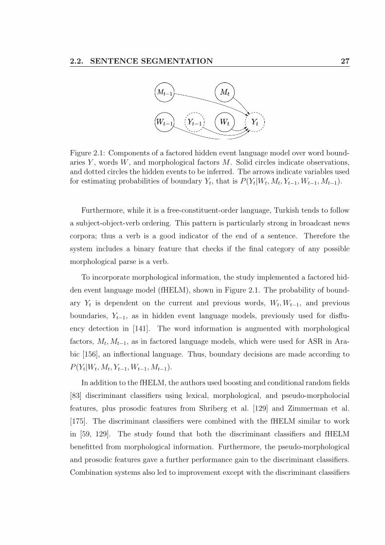
2.2. SENTENCE SEGMENTATION 27
Figure 2.1: Components of a factored hidden event language model over word bound-aries Y , words W , and morphological factors M . Solid circles indicate observations,and dotted circles the hidden events to be inferred. The arrows indicate variables usedfor estimating probabilities of boundary Yt, that is P (Yt|Wt,Mt, Yt−1,Wt−1,Mt−1).
Furthermore, while it is a free-constituent-order language, Turkish tends to follow
a subject-object-verb ordering. This pattern is particularly strong in broadcast news
corpora; thus a verb is a good indicator of the end of a sentence. Therefore the
system includes a binary feature that checks if the final category of any possible
morphological parse is a verb.
To incorporate morphological information, the study implemented a factored hid-
den event language model (fHELM), shown in Figure 2.1. The probability of bound-
ary Yt is dependent on the current and previous words, Wt,Wt−1, and previous
boundaries, Yt−1, as in hidden event language models, previously used for disflu-
ency detection in [141]. The word information is augmented with morphological
factors, Mt,Mt−1, as in factored language models, which were used for ASR in Ara-
bic [156], an inflectional language. Thus, boundary decisions are made according to
P (Yt|Wt,Mt, Yt−1,Wt−1,Mt−1).
In addition to the fHELM, the authors used boosting and conditional random fields
[83] discriminant classifiers using lexical, morphological, and pseudo-morpholocial
features, plus prosodic features from Shriberg et al. [129] and Zimmerman et al.
[175]. The discriminant classifiers were combined with the fHELM similar to work
in [59, 129]. The study found that both the discriminant classifiers and fHELM
benefitted from morphological information. Furthermore, the pseudo-morphological
and prosodic features gave a further performance gain to the discriminant classifiers.
Combination systems also led to improvement except with the discriminant classifiers

28 CHAPTER 2. BACKGROUND
with all features.
Kolar et al. [82] faced a similar problem with the highly inflectional and deriva-
tional nature of Czech. The study used a positional tag system that consisted of a
string of 15 symbols to denote the morphological category of each word, resulting in
1362 distinct tags in their training data. While the language model using tag data
did not perform as well as the word-based model, they found the system benefitted
from replacing infrequent words and out-of-vocabulary words in testing with subtags
consisting of a subset of 7 symbols. This reduced the language model vocabulary from
295k words to 62k mixed words and subtags. The work also used prosodic features
borrowed from Shriberg et al. [129].
Batista et al. [7] and Batista et al. [8] have studied punctuation detection in Por-
tuguese and, to a lesser degree, Spanish. [8] compared the detection of the two most
common punctuation, full stops and commas, in English, Portuguese, and Spanish.
The model used was a maximum entropy (ME) model using eight word LMs up to
trigrams and the eight corresponding LMs using parts of speech, pause duration, and
speaker and gender change events. In comparing the slot error rate between the three
languages, they note that overall performance is weighted toward the more common
comma, which is generally a harder problem because commas serve multiple purposes.
The Portuguese data suffered from inconsistent annotation and a greater proportion
of spontaneous speech. The spontaneous speech, being more unstructured, has a
higher word error rate, which is an issue for a system heavily dependent on lexical
data.
[7] extended their work on Portuguese punctuation by adding prosodic features
and question mark detection. The prosodic features used are based on Shriberg
et al. [127, 129], though pitch and energy features are extracted over syllable and
phone regions in addition to word regions. This interest in other linguistic units is
motivated by linguistic findings [41], especially in stressed and post-stressed syllables.
However, they find that word pitch followed by word energy features are the most
useful, in that order, and combination with syllable features does not lead to further

2.2. SENTENCE SEGMENTATION 29
improvement. They partially corroborate the findings in [127] on the contribution
and language-independence of various prosodic features.
The primary language specific issues discovered were in pitch and duration. Dif-
ferent pitch slopes are suspected of being associated with discourse functionalities
beyond sentence structure. As for duration, the literature reports three segmental
strategies at the end of intonational phrases: “epenthetic vowel, elongated segmental
material, or elision of post-stressed segmental material” [7]. However, there are no
existing features that quantify these events, and the duration features used by the
system helped little. Pre-boundary lengthening was observed in Portuguese.
Kawahara et al. [72] extended their previous work on Japanese sentence and clause
units by using local syntactic information. Because subjects and objects may be
omitted in spontaneous Japanese, the definition of a sentence is not well-defined, and
the study relied on a human annotation of three different boundary strengths. The
dependency structure used is based on minimal grammatical units called bunsetsu
consisting of one content word and adjacent functional words. Dependency is usually
left-to-right with the predicate in the final position of the sentence. To extract this
dependency structure, the study used a chunking algorithm to chunk words into bun-
setsu units, determine dependency between adjacent bunsetsu, and determine whether
a bunsetsu is a predicate. Separate classifiers were trained for each step, using surface
forms, baseforms, and POS tags.
Both their baseline and proposed systems consisted of voting pairwise SVMs
trained on the surface forms and POS tags of the three words before and three words
after the candidate boundary. While in the baseline system every word-final bound-
ary was considered a candidate boundary, the proposed system restricted candidate
boundaries to edges of the generated chunks. They found that the syntactic chunk-
ing improved the detection of boundaries in ASR output, though is some confusion
between different boundary strengths.

30 CHAPTER 2. BACKGROUND
2.3 Feature Selection
Feature selection is the process of selecting a subset of features toward some ob-
jective, such as improving the performance of the learning algorithm that uses them.
The benefits of a smaller feature set include:
• Reducing computation time and resources
• Avoiding overfitting model parameters by having more data per parameter
• Making data interpretation and visualization easier
Blum and Langley [14], Guyon and Elisseeff [55], and Saeys et al. [119] provide
good overviews of feature selection methods.
2.3.1 Filters and ranking
Filtering and ranking are methods of scoring features according to their usefulness,
either as the primary feature selection method or in aid of one. Filtering in the
literature usually considers each variable independently, which makes them fast and
linearly scaling with the number of features, but unable to consider feature interaction.
Being classifier independent has the same trade-off as generalist approaches, aiming
to be good for any given classifier selected but not guaranteed to be optimal for any.
Often, filtering performs well enough to act as a baseline feature selection method.
Common ranking criteria. The correlation coefficient between input random
variable Xi and outcome random variable Y is:
Ri =cov(Xi, Y )√var(Xi)Y
However, since the distributions of these random variables are unknown, the variances
and covariance are estimated from the data. In the context of linear regression, R2i is
the proportion of the total variance of outcome Y that can be explained by feature
Xi. Correlation criteria can be extended beyond linear fitting by performing a non-
linear transformation — for example, taking the log of or squaring the variable — or

2.3. FEATURE SELECTION 31
performing a non-linear regression and ranking the features by goodness of fit. To
use correlation coefficients for binary classification, the two class labels are assigned
values of y, typically ±1, in which case it resembles Fisher’s, T-test, and similar
criteria [44, 50, 62, 151].
Related to the idea of selecting features based on their goodness of fit, the analogue
in classification would be sorting variables by their predictive power. For binary clas-
sification, a single-variable classifier can be created by placing one decision threshold,
labeling all instances of the variable above the threshold as one class and examples
below as the other class. Adjusting the threshold trades off the false positive and
false negative error rates; common characterizations used for error curves are the
equal error rate point and area under the ROC curve.
Other filtering criteria stem from information theory [10, 30, 36, 150], many based
on the mutual information between the variable x and the target y:
Ii =
∫xi
∫y
p(xi, y) logp(xi, y)
p(xi)p(y)dxdy
In the case of discrete features and targets, estimating the marginal and joint distri-
butions is a matter of counting. However, with continuously-valued variables, their
distributions need to be estimated, for example by discretization or approximating
their densities [150].
Redundancy. One consequence of analyzing features separately without consid-
ering their interaction is the possibility of selecting redundant features. From an in-
formation theory point of view, redundant information cannot improve performance
if there is no new information to improve decision making. However, in practice,
learning algorithms might not fully utilize the information content of the input vari-
ables because of the limitations of their models and the features themselves may have
observation error. Thus redundant features can improve performance through noise
reduction.
Variable interaction. Another issue of ignoring feature interaction is whether
two or more features, while individually not useful, may together have predictive
ability. As a toy example to show this is possible, Guyon and Elisseeff [55] give an
example where for one class label features (x1, x2) have a bimodal normal distribution

32 CHAPTER 2. BACKGROUND
about (1, 1) and (−1,−1) with equal probability, and the other class label has a
similar distribution centered around (1,−1) and (−1, 1). From the perspective of
either variable xi, both classes have the same distribution about 1 and -1, but taken
together the four modes are separable. Note that this example is commonly used in
probability and statistics texts to show that independence does not imply conditional
independence, in this case the variables being not conditionally independent given
the class label.
2.3.2 Subset selection methods
As opposed to filtering, which examines each feature independently of the oth-
ers, feature subset selection methods seek to find a set of features that optimizes an
objective function, often the performance of a particular learning algorithm, some-
times with a regularization term to penalize large feature sets. For N variables, an
exhaustive search over all 2N − 1 proper subsets is only practical for small N ; thus
these methods focus on algorithms that efficiently search the space of possible feature
subsets.
Wrappers
Wrappers obviate the need to model the learning algorithm by treating it as a
black box. Instead, different feature subsets are presented to the learning algorithm,
and the fitness of a feature subset is based on the learning algorithm output. Various
algorithms can be employed to efficiently search the space of variable subsets, and
some common ones are detailed below. There is a trade-off between efficient search
strategies and system performance, but Reunanen [113] among others notes that
coarse search algorithms may reduce overfitting the feature subset to the training
data.
Two commonly used search paradigms are forward selection and backward elimi-
nation. Forward search begins with an empty feature set and iteratively adds more.
Backward elimination does the reverse, starting with all features and gradually remov-
ing them. See Figure 2.2 from [81]. In their simplest incarnations, these algorithms

2.3. FEATURE SELECTION 33
Figure 2.2: The search space of a feature selection problem with 4 features. Each nodeis represented by a string of 4 bits where bit i = 1 means the ith feature is included and0 when it is not. Forward selection begins at the top node and backward eliminationbegins at the bottom node, with daughter nodes differing in one bit.
are greedy searches that explore all possible daughter nodes, e.g. in forward selection,
the current feature subset plus each unselected feature individually. The highest
scoring daughter then becomes the parent node explored in the next iteration.
The concern with greedy algorithms is falling into local maxima, either due to
pruning a path that would lead to the global maxima or a stopping condition ending
the search too early. Kohavi and John [81] show that best-first search [118] achieves
more robustness than hill-climbing by making a couple alterations, namely instead of
exploring only the best node, maintaining a set of nodes that are within a margin of
the current best score and altering the stopping criterion by increasing the number of
iterations without progress required before stopping. Empirical evidence suggests that
greedy search is computationally efficient while being robust to overfitting. For further
variants on forward and backward search, including beam search and bidirectional
search see [111, 131].
The primary trade-off in forward versus backward search is that, while backward
elimination may capture feature interaction, training models with large features sets
can be computationally expensive. [80] proposes that backward search can be sped
up through compound operators. For example, if past iterations have shown the
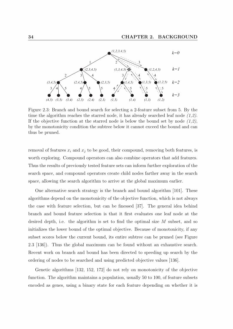
34 CHAPTER 2. BACKGROUND
Figure 2.3: Branch and bound search for selecting a 2-feature subset from 5. By thetime the algorithm reaches the starred node, it has already searched leaf node (1,2).If the objective function at the starred node is below the bound set by node (1,2),by the monotonicity condition the subtree below it cannot exceed the bound and canthus be pruned.
removal of features xi and xj to be good, their compound, removing both features, is
worth exploring. Compound operators can also combine operators that add features.
Thus the results of previously tested feature sets can inform further exploration of the
search space, and compound operators create child nodes farther away in the search
space, allowing the search algorithm to arrive at the global maximum earlier.
One alternative search strategy is the branch and bound algorithm [101]. These
algorithms depend on the monotonicity of the objective function, which is not always
the case with feature selection, but can be finessed [37]. The general idea behind
branch and bound feature selection is that it first evaluates one leaf node at the
desired depth, i.e. the algorithm is set to find the optimal size M subset, and so
initializes the lower bound of the optimal objective. Because of monotonicity, if any
subset scores below the current bound, its entire subtree can be pruned (see Figure
2.3 [136]). Thus the global maximum can be found without an exhaustive search.
Recent work on branch and bound has been directed to speeding up search by the
ordering of nodes to be searched and using predicted objective values [136].
Genetic algorithms [132, 152, 172] do not rely on monotonicity of the objective
function. The algorithm maintains a population, usually 50 to 100, of feature subsets
encoded as genes, using a binary state for each feature depending on whether it is

2.3. FEATURE SELECTION 35
included or not. The idea is for the population to improve with each iteration of
evolutionary pressure by culling the weaker genes. There must be at least one way
for genes to adapt, such as crossover (genes copy or swap portions of their code)
or mutation (random flips in the state of a feature). Such adaptation is random
but designed to keep child genes similar to their parent(s). A decision must also
be made as to how to select which genes survive to the next generation, such as
only keeping the top N genes or making survival probability a function of rank or
fitness. The strength of genetic algorithms is that, by maintaining a sufficiently large
population, they can be robust to local maxima, evaluate the fitness of large areas of
the search space simultaneously, and pass on that information to the next generation,
thus getting close to the global maxima fairly quickly. However, since mutation is
random and not always intelligent, there is no guarantee the algorithm will find the
global optimum.
Related to genetic algorithms is simulated annealing [73, 89, 132], which is named
after a metallurgical process where atoms in a metal, if heated hot enough and cooled
slow enough, will crystlize into a low-energy state. To translate this to the opti-
mization problem of feature selection, the current solution is perturbed, similar to
mutation in genetic algorithms. If this results in a better objective function, it re-
places the current solution. Otherwise, there is a probability that it replaces the
current solution anyway depending on how much the objective function drops, typi-
cally proportional to e−∆T , where ∆T is the change in “temperature,” i.e. objective
function. In this way, the algorithm tends to follow the slope of the search space, but
occasionally goes against it, which allows it to escape local maxima. A key decision
is setting the probability that the algorithm accepts a lower objective function: if set
too high, it regresses too often and is slow to converge; if set too low, it is more prone
to local minima.
Embedded methods
As opposed to wrappers, embedded methods integrate feature selection into the
learning algorithm. Some algorithms, such as CART-style decision trees [16] and the

36 CHAPTER 2. BACKGROUND
AdaBoost classifier [38] I use in this thesis, have them built in. For example, at each
node, the decision tree selects the single best feature to split the data with. The
primary benefit of embedded methods over wrappers is that they need not train a
new model for each potential feature set and so are faster.
For instance, [56] examined backward elimination for a support vector machine
(SVM) with a linear kernel. Assuming the SVM parameters remain the same, the
linear kernal allows the algorithm to quickly estimate the change in the objective
function caused by removing individual features. Backward elimination removes the
lowest ranking variable in each iteration. The study found the nested feature sets pro-
duced by this method to be more robust to overfitting, like those found by forward
selection and backward elimination wrappers, especially when compared to combina-
torial searches, i.e. exhaustively searching all subsets with a maximum size.
Other methods of predicting the change due to removing each variable include:
sensitivity [107]; using the derivative of the objective function with respect to the
variable or weight; and quadratic approximation [116] using a second-order Taylor
expansion of the objective function 12∂2J∂w2
i(wi)
2, an idea borrowed from the optimal
brain damage method to prune neural network weights [85]. Pruning neural networks
is also a form of feature selection, reducing the number of active inputs to a node.
The reasoning behind the second-order expansion is that, when objective function J
is optimal, the first-order terms can be neglected.
SVMs can use objective functions with regularization terms to penalize the number
of variables. These models also perform feature selection as part of their optimization.
For linear SVMs with weights w, a commonly used regularization term is the lp-
norm, ‖w‖p = (∑n
i=1wpi )
1/p. Weston et al. [161] show that l0-norm regularization,
which is a penalty term proportional to the number of the non-zero weights, can be
approximated by iteratively training an l1- or l2-norm SVM and rescaling the input
variables by their weights. Bi et al. [12] show that l1-norm SVMs can be approximated
without the iterative process using an approach similar to that used by [148] for least-
squares regression.

2.3. FEATURE SELECTION 37
2.3.3 Feature construction
An alternative to selecting a subset of input variables is to extract features from
them with the purpose of improving learning algorithm performance and/or dimen-
sionality reduction without losing the information content of the original variables.
One common method of feature construction is forming linear combinations of the
input variables. I cover linear discriminant analysis (LDA), using supervised learning
to extract discriminant features, in Sections 4.1.1 and 4.1.2. Unsupervised learning
transforms seek to compress the data with minimal loss. For example, principle
component analysis (PCA) creates an orthogonal basis where the first component
captures as much variance of the original variables as possible, and each successive
component does the same under the constraint of being uncorrelated with previous
components. Singular value decomposition (SVD), lifting the orthogonality condition,
provides the reconstruction with minimal least squares error [31]. Depending on
the data, other forms of data decomposition such as Fourier, Hadamard, or wavelet
transforms may be applicable.
More recently, Globerson et al. [47] proposed an unsupervised feature construction
method called sufficient dimensionality reduction that extracts the most informative
features, which maximizes what they call information in the measure. This builds on
their previous work on the information bottleneck method [149], which seeks to find
the best trade-off between reconstruction and compression for a random variable.
They show that the feature construction is the dual of the reverse feature design
problem and equivalent to a Kullbeck-Leibler (KL) divergence minimization problem,
which they solve by an iterative projection algorithm. However, it appears this work
has not been extended to multiple output features.
Another method in feature construction is to cluster similar variables and replace
them with a centroid feature. Duda et al. [31] covers basic approaches using K-means
and hierarchical clustering. To give an example, document and text classification of-
ten uses word counts as variables under a bag-of-words model, but then the size of
the variable set is equal to the size of the vocabulary. Baker and McCallum [6] and
Slonim and Tishby [134] clustered word variables according to the their distribu-

38 CHAPTER 2. BACKGROUND
tion across document classes, varying in their methods for clustering and extracting
features from word clusters, Slonim and Tishby using the previously mentioned in-
formation bottleneck method. These methods maintain discriminatory information
between document classes better than unsupervised learning with latent semantic
analysis [29], which compresses word variables by using an SVD decomposition of
word frequency across documents.

39
Chapter 3
Feature Robustness
This chapter provides the motivation for the experiments in Chapters 4 and 5. It
examines the robustness of an existing set of prosodic features originally designed for
English when ported without any changes to other languages, specifically Arabic and
Mandarin. Beyond looking at the performance gains from adding prosodic features to
lexical information, I use feature selection methods to compare how specific features
and categories of features perform across the different languages.
What we shall see is that the feature set, which has been designed to be word-
independent and have multiple similar features backing each other up, is fairly robust
to different language conditions. However, beyond the ubiquitous pause feature, this
redundancy makes it fairly difficult to predict a priori how useful any particular
feature will be or which feature should be next chosen by the feature selection al-
gorithm. One of the stronger patterns found was that the pitch features performed
significantly worse in Mandarin than in Arabic or English, which is believed to be
due to Mandarin lexical pitch interfering with the manner in which the pitch features
are designed. This leads to the question of how a researcher should set out to design
a good set of features, a question I will take up in Chapter 4.

40 CHAPTER 3. FEATURE ROBUSTNESS
3.1 Background
3.1.1 Feature set history and applications
The prosodic feature set studied in this chapter is the work of Shriberg. It can
trace its origins to a 1997 paper on using only prosodic information for disfluency
detection [126]. There, Shriberg et al. successfully found cues in segemental duration
and pitch in the detection and classification of disfluencies, such as filled pauses
and false starts. The design of the pitch features to measure pitch dynamics across
a boundary is similar to what is described in Section 3.1.1, as are what elements
the pause and segmental duration features attempt to quantify. Also, they have
in common the use of both normalized and raw versions of the pitch and duration
features.
This work was expanded in Sonmez et al. [137], which applied the features to the
speaker verification task. Here, the pre-processing of the pitch vector is refined, using
the lognormal tied mixture (LTM) model [138] to remove halving and doubling errors
from the pitch tracking software. Furthermore, the LTM model provides speaker
parameters that can be used for speaker normalization. This is followed by a median
filter to smooth out microintonation effects and fitting piecewise linear segments to
the pitch vector, called piecewise linear stylization in the literature. As a result of this
smoothing, the authors were able to improve performance by adding to the existing
short-term cepstrum spectra more long-term features describing the pitch contour. It
should be noted that this pre-processing was also carried over to the energy features
when they were introduced.
Since then, the feature set has been used in a wide variety of applications. For
speaker recognition [128], the features were not used by the learning algorithm di-
rectly, but feature events were counted over syllable-based regions. This discretization
could then be put in N -grams, which were the features used by the SVM learner, simi-
lar to what was done by Adami et al. [3]. The features have also been used to estimate
the fluency of language learners [145], primarily checking to see that word stress was
properly executed by measuring vowel duration and maximum pitch excursion.

3.1. BACKGROUND 41
The features are able to capture emotion and have been used in several related
tasks. Ang et al. [4] used the features, along with a language model and speaking style
labels, to detect annoyance or frustration in users making air travel arrangements
using an automatic telephone service. They found that long segmental duration,
slower speaking rate, and high pitch peaks were indicative of annoyance. Hillard
et al. [63] used what they called an unsupervised learning method, though more
accurately it could be described as semi-supervised co-training, to cluster meeting
spurts using language models into agreement, disagreement, backchannel, and other.
A decision tree classifier using the prosodic features and word-based features was
then trained on this automatically labeled data. The study found that the prosodic
features performed almost as well as the word-based features, which included positive
and negative keywords, but their combination showed little improvement. On the
same meeting data, Wrede and Shriberg [164] found that some prosodic features were
highly correlated with speaker involvement, which is indicative of meeting hot spots.
In particular, speaker normalized pitch features involving mean or maximum were
strong features, while pitch range, energy, and unnormalized features were less so.
However, due to difficulties with human labeler agreement, the study did not have
data to train a reliable classification system and so stopped at feature ranking.
Many of the sentence segmentation systems covered in Section 2.2.4 [26, 57, 59,
96, 129, 175] used these features, often combined with a language model. While
pause duration overwhelmingly yields the most predictive set of features for detecting
sentence boundaries, pitch and segmental duration features contribute significantly
to overall performance. Shriberg et al. [129] also studied the use of these prosodic
features in topic segmentation of broadcast news, finding similar feature usage as in
their broadcast news sentence segmentation decision trees, including the importance
of pause duration, though pitch range features were especially prominent. Ang et al.
[5] used pause duration to segment dialog acts in meetings and then used the prosodic
features to train a decision tree to classify the segments. The posterior probability of
the prosodic decision tree was then used as the input to a maximum entropy classifier
to incorporate lexical data. The study did not report which prosodic features were
most useful, but the authors noted that ASR errors impaired the lexical-based model

42 CHAPTER 3. FEATURE ROBUSTNESS
much more than the prosody-based model.
To summarize, this set of prosodic features has been used in a spectrum of different
tasks. Rather than design new features for each new task for various cues, the features
were used off the shelf, though Shriberg has modified and added to the feature set over
time. Thus this feature set can be viewed as a good general-purpose set of prosodic
features, quantifying a wide variety of prosodic behavior and leaving the learning
algorithm to determine how to best make use the information.
The above studies have a number of points in common. Firstly, all of them used
English data, and the following work was the first to study its portability to other
languages. Secondly, many showed that prosodic information improved performance
when added to lexical data, showing that they are complementary. Furthermore,
many noted that word-independence is a positive property of the feature set. While
the prosodic features do require word alignments, and for many corpora these were
taken from ASR outputs, the word-independence made the prosodic features more
robust to transcription errors than language models. Among the prosodic features,
the most lexically dependent ones are the segmental duration features, which rely
on the time alignments of vowels and rhymes. While sonority makes it easier to
locate vowels than identify them, phone identities are used to calculate the mean and
variance parameters used for segmental duration normalization.
The following describe the features used for this dissertation. For more precise
details about the construction of individual features, see [34]. The following feature
extraction was done in Algemy, a Java-based prosodic feature extraction system cre-
ated by Harry Bratt at SRI International [15] (see Figure 3.1). The idea behind
Algemy is that many prosodic feature extraction algorithms share common building
blocks. For example, taking the mean value of frames within a window, finding which
values exceed a threshold, or performing a regression or normalization over a set of
frame/window values. However, prosodic feature extraction algorithms are typically
written like any other computer program, leaving the author to code the operations
and manage data streams themselves. This has the drawbacks usually related to com-
puter programming, including the difficulty of reading and reusing code from other
researchers. Algemy contains a graphical user interface which allows a researcher to

3.1. BACKGROUND 43
Figure 3.1: A screenshot of the Algemy feature extraction software. Note the modularblocks used for the graphical programming of prosodic features and handling of datastreams. The center area shows the pitch and energy pre-processing steps.
create prosodic feature extraction algorithms using a graphical programming language
with a wide variety of pre-made blocks.
The benefit of Algemy is that, once the learning curve has been crested, the
prototyping of prosodic features using the provided blocks is very quick. It is also
easy to comprehend and edit algorithms. In batch mode, feature extraction is as
fast and memory efficient as traditional C++/Java implementations. The downsides
to Algemy include its learning curve, especially as one needs to be familiar with
what blocks are available and their function to become proficient in their usage. If
a particular functionality is not available, users can code contributions to the library
of blocks, as I did for this project.

44 CHAPTER 3. FEATURE ROBUSTNESS
Pause
Pauses often mark the boundaries between language units, such as sentences and
topics. This is especially true in broadcast news, where pause cues help the audience
follow the news item, relative to spontaneous speech where pauses may occur due to
speakers reacting to one another or thinking of what to say next. The pause duration
feature used is the inter-word times as given by the ASR output, many of which are
zero during continuous speech. The feature set also includes the pause duration for
the previous two and the next inter-word boundaries, making four pause features in
total. These additional features inform the classifier of whether there is a break in the
vicinity, which reduces the likelihood of a sentence boundary at the current boundary.
Pitch
The pitch features can be broadly classified into three categories: range, reset,
and slope features, which are described individually below. All of the pitch features
go through the following pre-processing steps. Fundamental frequency values are ex-
tracted using the ESPS pitch tracker get f0 [1] in 10ms frames over voiced speech.
Pitch trackers commonly suffer from halving and doubling errors, where the tracker
believes the speaker to be an octave above or below their actual pitch. A lognor-
mal tied mixture (LTM) model [138] is employed to detect and remove these errors.
Each speaker model consist of three lognormal components with equal variances and
means tied log(2) apart on the lognormal scale. An expectation maximization (EM)
algorithm estimates the mean, variance, and mixture weight parameters. Not only
does this fix most halving and doubling errors, the speaker model provides speaker
baseline and range parameters for normalization, including speaker mean, baseline
and topline — located between the middle mode and halving and doubling modes,
respectively.
Further pitch pre-processing includes a 5-frame median filter, which smoothes out
pitch instability during voicing onset, followed by a process called piecewise linear
stylization first used in [137]. A greedy algorithm fits piecewise linear segments to
the pitch contour (see Figure 3.2), minimizing mean square error within the constraint

3.1. BACKGROUND 45
Figure 3.2: An example of the piecewise linear stylization of a pitch contour, in thiscase from Mandarin. The blue dots are the pre-stylization pitch values while thegreen lines show the piecewise linear segments. The horizontal axis is in 10ms frameswith the purple blocks on the bottom showing words. Notice that while stylizationtends to conform to word boundaries, the pitch contour for word A has been absorbedby the words around it and one long linear segment crosses boundary B.
of a minimum segment length. This removes microintonation and also extracts pitch
slope values that are used in the pitch slope features.
From this stylized pitch, five pitch statistics are extracted over each word: the
first and last stylized pitch values plus the maximum, minimum, and mean stylized
pitch over the word. These statistics are similar to the prosodic features used in
[33, 143, 165, 171], measuring the distribution of the pitch values. However, Shriberg
derives features from these pitch statistics as explained below.
Range features. The range features quantify how far the word departs from the
speaker’s usual speech patterns. For instance, toward the end of sentences speakers
tend to drop toward the lower end of their range. In the range features, the pitch
statistics extracted above are compared to speaker baseline and topline parameters
taken from the LTM models. These comparisons include both absolute differences
and log-ratios, some normalized by the speaker LTM range parameter. To classify a

46 CHAPTER 3. FEATURE ROBUSTNESS
boundary, range features are taken from both the words before and after the boundary
in question, though [129] notes that the features are not symmetric, and in sentence
segmentation there is preference for range features from the word before the bound-
ary. Because these are important to the work in Chapters 4 and 5, they are detailed
in Appendix A.3.
Reset features. One of the strongest pitch cues, at least in English, for the end
of one syntactic unit is a drop in pitch followed by a pitch reset to start the next
unit from a higher point [142]. To calculate these, the same five statistics from the
stylized pitch contours over word segments were used, in this case comparing one
statistic from each word on either side of the boundary in question. Like the range
features, these comparisons used absolute pitch difference, log-ratios, and speaker
normalization. These features are detailed in Appendix A.2.
A large number of features were extracted to quantify pitch reset. Not just com-
paring the last pitch of the word before the boundary to the first pitch of the word
after, which may be susceptible to voicing or pre-processing steps, but all combi-
nations of the maximum and minimum of both words as well as comparing their
means are included, which capture a variety of possible word contours. Furthermore,
many of these features were duplicated, except using statistics pulled from the 200ms
windows before and after the boundary. The length of the 200ms window was deter-
mined empirically through experiments but is approximately the length of an English
syllable.
Note that the range and reset pitch features, except the 200ms reset features, are
constructed from the same five pitch statistics extracted over each word, plus some
LTM speaker parameters. These will form the basis for the automatic pitch feature
design in Chapters 4 and 5.
Slope features. The pitch slope features describe pitch trajectory around the can-
didate boundary from the slope of the piecewise linear pitch stylization. Specifically,
the last pitch slope before and first slope after the boundary are extracted, as well
as a continuity feature based on the difference between the two. Because stylization

3.1. BACKGROUND 47
occurs independently of word boundaries, the piecewise linear segments may extend
across words as seen at boundary B in Figure 3.2, in which case the boundary is un-
likely to be a sentence break. If a linear segment encroaches into a neighboring word
for a few frames by some happenstance of the stylization or word time alignments,
those pitch slopes are not attributed to the word.
The pitch slope pattern features used for speaker recognition [3, 17, 114] could not
be implemented in Algemy at this time, so they were excluded from these sentence
segmentation experiments.
Energy
The energy features undergo pre-processing exactly like the pitch features: frame-
level RMS energy values are extracted using the ESPS toolkit, median filter, followed
by piecewise linear stylization. The LTM model is not used to fix halving/doubling
errors, as energy tracker outputs do not have a tri-modal distribution, but is used to
derive speaker energy parameters for normalization. This parallel feature extraction
allowed [3] to model pitch and energy contour dynamics over approximately syllable-
sized regions the same way. However, while pitch reset features are designed to
quantify a well-known pitch cue, the energy range and reset counterparts are more
intended to capture general energy behavior.
Segmental duration
A process called preboundary lengthening causes speech to slow down toward
the end of syntactic units [162], in particular affecting syllable nucleus and/or rhyme.
Thus the segmental duration features measure the lengths of the last vowel and rhyme
preceding the boundary in question. For example, the vowel duration features use
two normalizations, Z-normalization and ratio with respect to the mean. For normal-
ization, both speaker-specific parameters and those extracted over the entire corpus
are used. The rhyme duration features are similarly normalized with some feature
accounting for the number of phones in the rhyme, since syllable structures vary
between languages, with English allowing relatively complex rhymes [155].
48 CHAPTER 3. FEATURE ROBUSTNESS
Syllabification for these features is based on the phone string from the ASR output,
using the principle of coda maximization [71] and a list of phonologically allowed
codas built from training data. Note that the dependence on phones from recognizer
output, including the computation of the speaker and corpus phone parameters for
normalization, make these features less robust to ASR errors than the pitch and
energy features.
Speaker turns
While technically not prosodic features, these are included in the feature set be-
cause they are handled by the classifier in the same way. These features measure
time that has elapsed since the last speaker turn. In the absence of reference speaker
labels, speaker turns are extracted by automatic speaker diarization systems [163].
3.2 System
3.2.1 Classifier
The learning algorithm used for the following experiments is AdaBoost, a member
of the family of boosting algorithms [120]. The idea behind boosting is, instead of
training a single strong learner, to train a set of weak learners which collectively
perform well. The general approach in classification tasks is to iteratively reweight
the training data to emphasize examples that are currently being misclassified, and
train and add a weak classifier to address these trouble examples.
The software used, BoosTexter, is an extension of the AdaBoost algorithm [38] for
text categorization, which typically are multiclass (more than two possible classifier
labels) and multi-label (examples may belong to more than one class). Our research
uses BoosTexter primarily for its ability to handle both discrete and continuous fea-
tures, i.e. lexical and prosodic features respectively. The following experiments are
neither multiclass nor multi-label, so the algorithm effectively is the original Ad-
aBoost algorithm and will be referred to as such. The AdaBoost algorithm is trained
as follows: for N labeled examples {(x1, y1), . . . , (xN , yN)}

3.2. SYSTEM 49
• Initialize weight vector w1 comprised of weights w1i for each example i =
1, . . . , N . Typically, set all weights equal, wi = 1/N .
• Do for iteration t = 1, . . . , T :
1. Set example distribution:
pt =wt∑Ni=1w
ti
2. Call weak learnerW , providing it with distribution pt. Get back a hypoth-
esis ht : X → {0, 1}.
3. Calculate the error of ht : εt =∑N
i=1 pti|ht(xi)− yi|
4. Set βt = εt/(1− εt).
5. Set the new weight vector to be
wt+1i = wtiβ
1−|ht(xi)−yi|t
• Output hypothesis
hf (x) =
1,∑T
t=1
(log 1
βt
)ht(x) ≥ 1
2
∑Tt=1 log 1
βt
0, otherwise
AdaBoost training algorithm
Thus the overall classifier consists of T weak learners, ht, with associated weights,
log 1βt
. In the following experiments I used T = 1000 based on previous work [175].
It is possible to overtrain AdaBoost, and the general approach to prevent this is to
use held-out data to determine a good stopping point. However, given the number
of feature subsets tested during feature selection, it was not practical to continually
retrain the number of iterations, so T = 1000 was used throughout. The weak learners
used were CART trees with a single node, selecting the single feature and threshold
that minimize entropy in the daughter nodes, which can be trained fairly quickly.
Note that the weak learners are incapable of considering feature interaction.

50 CHAPTER 3. FEATURE ROBUSTNESS
The AdaBoost model produces a posterior score and, to perform classification, a
threshold must be set to separate sentence-final boundaries from non-sentence-final
boundaries. To tune this threshold parameter, a portion of the corpus called the
dev set, separate from the training data and evaluation data is held-out. Separate
thresholds are trained for F1 score and NIST error. The performance of the system
model is evaluated using the held-out eval dataset.
A support vector machine (SVM) classifier was considered as a comparison system
but was ultimately dropped from these experiments. The primary reason for this was
that an SVM classifier is sensitive to the setting of the cost parameters that govern
the trade-off between training error and margin. For the Mandarin experiments,
F1 score could range between 30% and 60% for even small parameter changes and
had no clear maxima, requiring the parameter to be readjusted for each feature set.
Similar parameter settings in English created swings no bigger than 1.5%, and I
believe the difference between the two languages to be due to the smaller size of
the Mandarin corpus. Thus, while the following experiments could also be run with
an SVM classifier, having to perform a parameter sweep for each feature set would
have greatly increased the runtime of the experiments. Since the AdaBoost classifier
outperforms SVM by several percent F1 score, I chose to drop SVM for the following
experiments.
3.2.2 Feature selection
Feature selection was performed to identify what prosodic features are useful in
the different languages. Specifically, if a feature or set of features performs well across
the three languages studied, this is a good indicator that the features are language-
independent. If so, those features and perhaps even the model trained on one language
can be ported to another, which may be useful if there is dearth of training data in
the target language.
To explore the relevance of the different prosodic features in each language, two
general feature selection methods were used: filtering and a forward selection wrapper,
which were described in more detail in Sections 2.3.1 and 2.3.2, respectively. The

3.2. SYSTEM 51
feature selection here serves two purposes: firstly, to optimize the performance of the
system; and secondly, to provide rankings and filtering measures that will allow us to
compare feature performance.
Filtering
In filtering, each feature is independently scored according to its usefulness in
predicting the class feature. Filtering is quick and simple, but it does not take into
consideration the learning algorithm or the interaction between features. Thus, it is
generally used to estimate feature relevance and filter out irrelevant features to speed
up more robust feature selection methods.
I used four different measures, as implemented in the Weka toolkit [60]: Chi-
Squared, Information Gain (3.1), Gain Ratio (3.2), and Symmetrical Uncertainty
(3.3). The latter three are related information theoretic measures [173]:
IG =H(class)−H(class|feat) (3.1)
GR =IG
H(feat)(3.2)
SU =2IG
H(class) +H(feat)(3.3)
where H(·) and H(·|·) are entropy and conditional entropy, respectively. The Chi-
Squared statistic measures the likelihood of the joint (class, feat) probability distri-
bution assuming a null hypothesis that they are independent.
Noting that the scores from these four measures are fairly correlated and follow
an exponential distribution, they were smoothed into one overall filtering score by
averaging them after mean normalization.
Forward selection
Forward selection is a type of wrapper, covered in more detail in Section 2.3.2.
Wrappers are feature subset selection algorithms that, unlike filtering, use the learning
algorithm by providing it feature subsets and using an objective function based on

52 CHAPTER 3. FEATURE ROBUSTNESS
the output to measure the fitness of the subset. The typical forward search wrapper
initializes the feature subset to an empty set and iteratively adds the feature that
improves performance the most. Hence, forward selection is a greedy algorithm and
as such may fall prone to local maxima. Furthermore, by considering only one feature
at a time, forward search ignores feature interaction until all but one are added to the
feature subset. Despite this, forward selection is generally very effective while being
computationally efficient and so is commonly used as a first pass at feature selection.
The forward search used in this study was a modified version of the N -best forward
search wrapper. At the time, there was still debate as to whether F1 score or NIST
error was the more reliable performance measure. At each iteration, a variable N
feature subsets were retained. The pruned subsets were those that were demonstrably
inferior, that is there exists one other feature subset in that iteration with a higher
F1 score and lower NIST error. Therefore the retained feature subsets can be ordered
in a progression of rising (improving) F1 score and rising (worsening) NIST error. In
addition to having the benefit of the N -best forward selection that it is more resilient
to the local maxima problem associated with a greedy search, the search space of the
modified algorithm includes that of forward search algorithms using each measure
separately since the subsets with the highest F1 score and lowest NIST error are
always retained.
A cousin to forward selection is the backward elimination wrapper, which is ini-
tialized with all features and iteratively removes the feature that contributes the least.
Because all features start included, backward search can see feature interations and
generally produces higher performance. However, because of the size of the feature
set and the fact that the time to train AdaBoost models increases at least linearly
with the number of feature, it is not always practical.
3.2.3 Corpus
To compare the performance of the prosodic feature set between languages, exper-
iments were run on a subset of the TDT-4 broadcast news corpus containing Arabic,
English, and Mandarin. Broadcast news data is largely read speech as opposed to

3.3. RESULTS AND ANALYSIS 53
spontaneous, with the reporter reading from a teleprompter. This type of speech
is more regular and has fewer speech disfluencies than spontaneous speech, such as
telephone conversations and meetings. Generally, speaker turns are fairly long, with a
reporter reading through their news item, though cutting to sound or video clips will
create shorter speaker turns. Interview-style segments within broadcast news behave
more like spontaneous speech.
The size of each dataset is shown in Table 3.1. For each language, the corpus was
split 80/10/10% between train, dev, and eval sets. As mentioned in Section 3.2.1,
the classifier posterior probability threshold is trained on the held-out dev set and
system performance is evaluated using the eval set.
ARB ENG MANNumber of words 185608 931245 459571
Avg. sentence length 21.5 14.7 24.7
Table 3.1: Corpus size and average sentence length (in words).
3.3 Results and Analysis
To motivate the use of prosodic features, Table 3.2 compares the result of all
prosodic features, a set of five lexical N -gram features, and their combination. Recall
from Section 2.2.3 that higher F1 score and lower NIST error rate indicate better
performance. We see that prosodic features can make significant contributions to
the sentence segmentation task. However, the Mandarin prosodic features perform
significantly worse than Arabic and English, both alone and when combined with the
lexical features.
3.3.1 Forward selection results
Figure 3.3 shows the performance of each iteration of the forward search exper-
iments for Mandarin. The figure is arranged to show both the F1 score and NIST
error rate of different feature subsets, with black lines marking the performance of
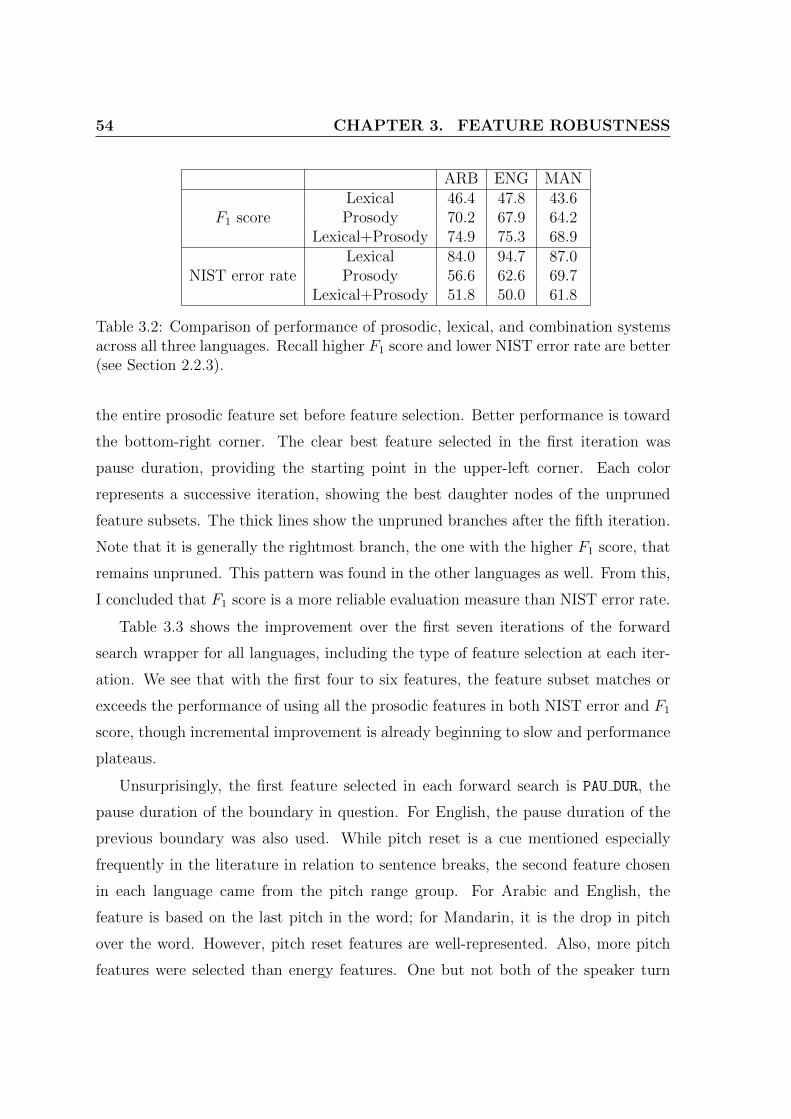
54 CHAPTER 3. FEATURE ROBUSTNESS
ARB ENG MANLexical 46.4 47.8 43.6
F1 score Prosody 70.2 67.9 64.2Lexical+Prosody 74.9 75.3 68.9
Lexical 84.0 94.7 87.0NIST error rate Prosody 56.6 62.6 69.7
Lexical+Prosody 51.8 50.0 61.8
Table 3.2: Comparison of performance of prosodic, lexical, and combination systemsacross all three languages. Recall higher F1 score and lower NIST error rate are better(see Section 2.2.3).
the entire prosodic feature set before feature selection. Better performance is toward
the bottom-right corner. The clear best feature selected in the first iteration was
pause duration, providing the starting point in the upper-left corner. Each color
represents a successive iteration, showing the best daughter nodes of the unpruned
feature subsets. The thick lines show the unpruned branches after the fifth iteration.
Note that it is generally the rightmost branch, the one with the higher F1 score, that
remains unpruned. This pattern was found in the other languages as well. From this,
I concluded that F1 score is a more reliable evaluation measure than NIST error rate.
Table 3.3 shows the improvement over the first seven iterations of the forward
search wrapper for all languages, including the type of feature selection at each iter-
ation. We see that with the first four to six features, the feature subset matches or
exceeds the performance of using all the prosodic features in both NIST error and F1
score, though incremental improvement is already beginning to slow and performance
plateaus.
Unsurprisingly, the first feature selected in each forward search is PAU DUR, the
pause duration of the boundary in question. For English, the pause duration of the
previous boundary was also used. While pitch reset is a cue mentioned especially
frequently in the literature in relation to sentence breaks, the second feature chosen
in each language came from the pitch range group. For Arabic and English, the
feature is based on the last pitch in the word; for Mandarin, it is the drop in pitch
over the word. However, pitch reset features are well-represented. Also, more pitch
features were selected than energy features. One but not both of the speaker turn

3.3. RESULTS AND ANALYSIS 55
Figure 3.3: An illustration of the performance of feature subsets during forward selec-tion for Mandarin. The horizontal axis shows F1 score while the vertical gives NISTerror rate with the two black lines showing the performance of the entire prosodicfeature set before feature selection. Colors correspond to feature selection iterations:1 provides the starting point, 2 magenta, 3 red, etc. The bold line shows whichbranches were not pruned by the 5th iteration. Note the preference for the rightmostbranch, which corresponds to the branch with highest F1 score.
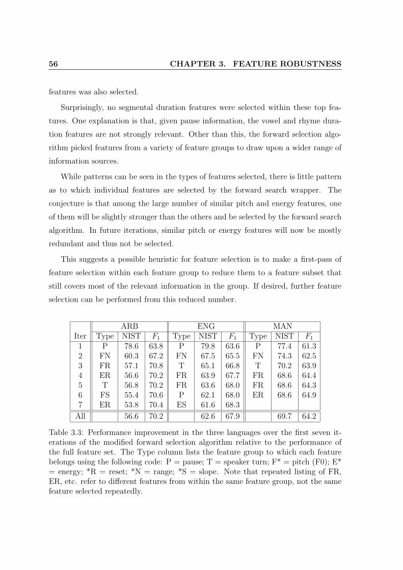
56 CHAPTER 3. FEATURE ROBUSTNESS
features was also selected.
Surprisingly, no segmental duration features were selected within these top fea-
tures. One explanation is that, given pause information, the vowel and rhyme dura-
tion features are not strongly relevant. Other than this, the forward selection algo-
rithm picked features from a variety of feature groups to draw upon a wider range of
information sources.
While patterns can be seen in the types of features selected, there is little pattern
as to which individual features are selected by the forward search wrapper. The
conjecture is that among the large number of similar pitch and energy features, one
of them will be slightly stronger than the others and be selected by the forward search
algorithm. In future iterations, similar pitch or energy features will now be mostly
redundant and thus not be selected.
This suggests a possible heuristic for feature selection is to make a first-pass of
feature selection within each feature group to reduce them to a feature subset that
still covers most of the relevant information in the group. If desired, further feature
selection can be performed from this reduced number.
ARB ENG MANIter Type NIST F1 Type NIST F1 Type NIST F1
1 P 78.6 63.8 P 79.8 63.6 P 77.4 61.32 FN 60.3 67.2 FN 67.5 65.5 FN 74.3 62.53 FR 57.1 70.8 T 65.1 66.8 T 70.2 63.94 ER 56.6 70.2 FR 63.9 67.7 FR 68.6 64.45 T 56.8 70.2 FR 63.6 68.0 FR 68.6 64.36 FS 55.4 70.6 P 62.1 68.0 ER 68.6 64.97 ER 53.8 70.4 ES 61.6 68.3
All 56.6 70.2 62.6 67.9 69.7 64.2
Table 3.3: Performance improvement in the three languages over the first seven it-erations of the modified forward selection algorithm relative to the performance ofthe full feature set. The Type column lists the feature group to which each featurebelongs using the following code: P = pause; T = speaker turn; F* = pitch (F0); E*= energy; *R = reset; *N = range; *S = slope. Note that repeated listing of FR,ER, etc. refer to different features from within the same feature group, not the samefeature selected repeatedly.

3.3. RESULTS AND ANALYSIS 57
From the results of the forward selection and filtering experiments, we wanted to
answer two questions:
1. Which features have low relevancy and can be removed from the forward search
without hurting performance?
2. How do different features perform across different languages?
3.3.2 Feature relevancy
The best single feature is PAU DUR. A sizable pause is a good indication that a
sentence has ended and a new one will begin. Another pause feature, PREV PAU DUR,
the duration of the pause of the previous boundary, has mediocre relevancy. For
TDT4-ENG, it is ranked 59th out of 84 features but was still selected in the forward
search wrapper, improving NIST error by 1.5% absolute on that iteration. Although
short sentences are not uncommon, it is more likely that a long PREV PAU DUR signals
that the previous boundary was a sentence boundary, which lowers the posterior
probability of the current boundary also being a sentence break.
It is clear that PREV PAU DUR contains nonredundant information in TDT4-ENG.
Two inferences can be drawn from this. First, even weakly relevant features can
contain useful information that the learning algorithm can exploit. Second, many
of the features originally ranked higher by filtering now contain mostly redundant
information by this early stage of the forward search wrapper. Thus, we conclude
that many of our features contain redundant information, and so the feature set
may benefit from feature selection. However, while some feature selection regimes
use filtering to remove irrelevant features and reduce the search space before using
a more sophisticated feature selection algorithm, in this feature set even low ranked
features are useful and should not be pruned.
Among turn-related features, TURN F and TURN TIME N are ranked very high by
filtering, and one of them was selected by the forward search wrapper in each language.
However, as TURN TIME N is a normalized version of TURN F, at that point the other
feature because almost entirely redundant. All other turn-related features performed

58 CHAPTER 3. FEATURE ROBUSTNESS
very poorly.
Pitch and energy features make up the bulk of the features selected by the for-
ward search wrapper, usually with more pitch features than energy. Filtering results
corroborate with this, with pitch features tending to score better than energy fea-
tures. This may be because pitch inherently has more useful information than energy
features, or it may be because of the design of our energy features. Despite energy
and pitch being two distinct entities, the extraction of the energy features involves
the same pre-processing, stylization, calculation of word-level statistics, and uses the
same templates for derived features.
Within the pitch features, the ones normalized by speaker pitch range generally
performed badly. In comparison, the features that were normalized using speaker
baseline pitch or another pitch value from the same speaker tended to do well and
were the ones selected by the forward search wrapper.
Pitch slope features tended to perform poorly, though we believe this is due to
the way they were calculated. Because the piecewise linear stylization operates in-
dependently of the transcript word time alignments, the piecewise linear segments
often do not coincide with the word boundaries. Thus, regions of uniform slope may
straddle a word boundary, as it is designed to if they appear to be part of the same
pitch gesture. While the system ignores segments that only extend 30ms or less into
a word, this appears to be insufficient. In this case, the feature that calculates the
difference in slope across the boundary will be zero.
3.3.3 Cross-linguistic analysis
Since the filtering scores varied considerably between languages, to compare fea-
ture performance across languages we examined their relative ranking as given by
filtering. The fifteen features that rose the most and dropped the lowest in compari-
son to other languages are summarized in Tables 3.4 and 3.3.3, respectively.
Mandarin clearly behaves differently from Arabic and English in terms of pitch
features. Pitch slope features perform exceptionally badly, which we attribute to Man-
darin being a tone language. Tone languages, which are explained in greater detail

3.3. RESULTS AND ANALYSIS 59
in Section 5.1.1, use pitch intonation to transmit lexical information. In Mandarin,
every syllable has one of four tones, and these lexical tones obscure sentence-level
pitch contours. The pitch slope features are calculated from the slopes of the piece-
wise linear stylization segments, which have a strong tendency to fit themselves to the
lexical tone contour. The other pitch features perform relatively better in Mandarin.
However, recall that the prosodic feature set performed worse in Mandarin than the
other languages.
The energy features are more difficult to interpret. For instance, in Arabic, a
number of cross-boundary energy features perform considerably better, and a number
perform considerably worse. Furthermore, while it appears that energy range and
energy slope do well in Arabic, more often than not this occurs because the same
features scored poorly in the other languages. We partly attribute this behavior to
the design of the energy features, which we plan to reexamine in future feature design
cycles.
While duration features clearly perform better in English than in the other lan-
guages, they were not selected in the forward search wrapper. This leads us to believe
that, while there is relevant information in the duration features, the features could
be designed better or they are largely redundant in the face of other features.
ARB ENG MANPitch range 2Pitch reset 8Pitch slope 3 3
Energy range 3Energy reset 4 1 5Energy slope 3
Duration (max) 6Duration (last) 5
Pause 1Speaker turn 1
Table 3.4: Feature groups of the top 15 features that ranked better in the languagenoted than the others.

60 CHAPTER 3. FEATURE ROBUSTNESS
ARB ENG MANPitch range 4 4Pitch reset 4 4Pitch slope 2
Energy range 4 1Energy reset 3 3 1Energy slope 1
Duration (max) 4 5Duration (last) 4 4
PauseSpeaker turn 1
Table 3.5: Feature groups of the top 15 features that ranked worse in the languagenoted than the others.
3.4 Conclusion
The original intention of this study was to show that the prosodic feature set
could make contributions in other languages besides English, which was demon-
strated, though the performance in Mandarin is considerably weaker than in Arabic
or English.
The forward selection results show classification systems benefit from a variety
of information sources. In particuar, pause duration is extremely useful, and cer-
tain speaker turn-related features were always selected. The remaining features are
drawn from a wide-variety of pitch and energy features. There is no consensus among
languages about which specific features are best. This may be explained by certain
feature groups having inherent redundancy, so once a feature from within the group
is selected, this makes the other features in the group less useful. Unexpectedly, no
duration features were selected, possibly because of redunancy with other features.
An analysis of the relevance of the features between different languages was also
performed. As a tonal language, Mandarin pitch features operate in a fundamentally
different manner than the other languages. While our energy and duration features
appear to work better in Arabic and English, respectively, certain behavior leads us
to believe we should also reexamine their design.

61
Chapter 4
Feature Extraction with HLDA
One of the objectives of this dissertation is to examine whether the feature de-
sign process can benefit from statistical learning methods. Automation may speed
up the feature design process, and a machine learning approach may be able to
learn language- or condition-specific behavior from data rather than have a human
researcher design features for them manually.
As mentioned in Section 3.1.1, up to the extraction of word-level pitch statistics,
the pitch features in Shriberg et al. [129] resemble pitch distribution features used in
[33, 143, 165, 171]. Shriberg et al. goes on to derive range and reset features as a
function of these statistics and LTM parameters.
This chapter attempts to derive its own features by applying heteroscedastic lin-
ear discriminant analysis (HLDA) to the same pitch statistics and LTM parameters.
Linear discriminant analysis (LDA) and closely related Fisher’s discriminant analy-
sis (FDA) are well-known methods in machine learning and statistics for perform-
ing a data transformation to improve the separation of different classes by finding
the linear transformation that maximizes between-class variance relative to within-
class variance. This provides a supervised learning method for the extraction of
prosodic features with discriminant ability. However, LDA makes an assumption of
homoscedascity, that all classes are distributed with the same covariance matrix. Het-
eroscedastic LDA, as the name implies, drops this assumption, though the underlying
idea of maximizing the separation of classes remains the same.

62 CHAPTER 4. FEATURE EXTRACTION WITH HLDA
4.1 Background
4.1.1 Linear discriminant analysis
Linear discriminant analysis (LDA) is a commonly used statistical method to find
linear combinations of features to separate the classes in labeled data. In Fisher’s
original article [35], he posed the question of what linear combination of four features
gave the maximum separation of the centroids of two classes of iris species relative to
the variance of the data. Let us define between-class scatter matrix as:
SB =K∑i=1
pi(µi − µ)(µi − µ)T
=K−1∑i=1
K∑j=i+1
pipj(µi − µj)(µi − µj)T (4.1)
where K is the number of classes, pi is the a priori probability and µi the mean of
the feature vectors of class i, and µ =∑K
i=1 piµi is the overall mean of the data. Also
define the within-class scatter matrix as:
SW =K∑i=1
piΣi
where Σi is the covariance matrix of class i. However, if we were to perform a linear
transform of the data, x = aTx, the corresponding scatter matrices would become
SB = aTSBa and SW = aTSWa. Thus Fisher’s original problem could be rewritten as
maxa
aTSBa
aTSWa
This is a generalized eigenvalue problem, and the optimal a is the eigenvector corre-
sponding to the largest eigenvalue of S−1W SB.
The above transform x = aTx projects the data into just one dimension. LDA
generalizes this to d output features by finding the d × n linear mapping A that
maximizes the Fisher criterion, which makes the homoscedasticity assumption that
all of the classes have the same variance Σ so that SW = Σ:
JF (A) = tr((ASWA
T )−1(ASBAT ))
(4.2)
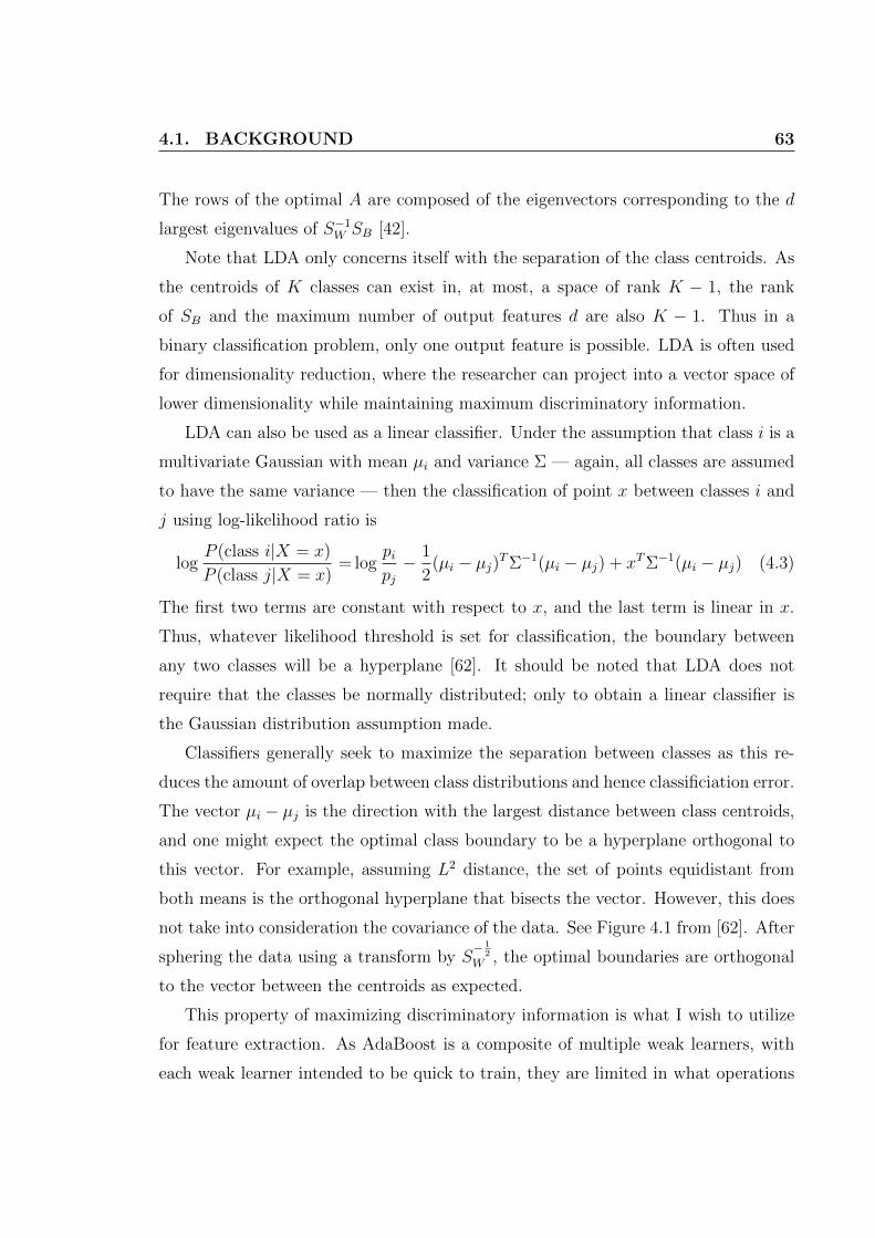
4.1. BACKGROUND 63
The rows of the optimal A are composed of the eigenvectors corresponding to the d
largest eigenvalues of S−1W SB [42].
Note that LDA only concerns itself with the separation of the class centroids. As
the centroids of K classes can exist in, at most, a space of rank K − 1, the rank
of SB and the maximum number of output features d are also K − 1. Thus in a
binary classification problem, only one output feature is possible. LDA is often used
for dimensionality reduction, where the researcher can project into a vector space of
lower dimensionality while maintaining maximum discriminatory information.
LDA can also be used as a linear classifier. Under the assumption that class i is a
multivariate Gaussian with mean µi and variance Σ — again, all classes are assumed
to have the same variance — then the classification of point x between classes i and
j using log-likelihood ratio is
logP (class i|X = x)
P (class j|X = x)= log
pipj− 1
2(µi − µj)TΣ−1(µi − µj) + xTΣ−1(µi − µj) (4.3)
The first two terms are constant with respect to x, and the last term is linear in x.
Thus, whatever likelihood threshold is set for classification, the boundary between
any two classes will be a hyperplane [62]. It should be noted that LDA does not
require that the classes be normally distributed; only to obtain a linear classifier is
the Gaussian distribution assumption made.
Classifiers generally seek to maximize the separation between classes as this re-
duces the amount of overlap between class distributions and hence classificiation error.
The vector µi − µj is the direction with the largest distance between class centroids,
and one might expect the optimal class boundary to be a hyperplane orthogonal to
this vector. For example, assuming L2 distance, the set of points equidistant from
both means is the orthogonal hyperplane that bisects the vector. However, this does
not take into consideration the covariance of the data. See Figure 4.1 from [62]. After
sphering the data using a transform by S− 1
2W , the optimal boundaries are orthogonal
to the vector between the centroids as expected.
This property of maximizing discriminatory information is what I wish to utilize
for feature extraction. As AdaBoost is a composite of multiple weak learners, with
each weak learner intended to be quick to train, they are limited in what operations

64 CHAPTER 4. FEATURE EXTRACTION WITH HLDA
Figure 4.1: The left figure shows the distribution of the two classes if they are pro-jected along the direction that maximizes the separation of the centroids. However,because the covariance of the distributions are not diagonal, the resulting distributionhas considerable overlap. In the right figure, the data is projected along a directiontaking into consideration the covariance. While the class means are closer together,there is less overlap and thus less classification error.
they can do on multiple features. In this system, AdaBoost uses single-node decision
trees, so it is difficult to exploit feature interation. The LDA transform extracts
feature combinations that should be useful for classification. This idea is not new, and
indeed is a common linear dimensionality reduction method used in image recognition
applications [11], such as face, landmark, or shape recognition. A common difficulty in
applying LDA to these tasks is the “small sample size” problem, where LDA becomes
unstable when the number of training samples is smaller than the dimensionality of
the samples [86, 95, 176]. However, this should not apply to the sentence segmentation
task.
4.1.2 Heteroscedastic LDA
As stated in Section 4.1.1, LDA makes the homoscedasticity assumption that all
classes have the same covariance matrix. In practice, even when the estimated class
covariance matrix from the data generally are not the same, all classes are treated
as having the covariance of the whole training set. One consequence of this is that
LDA cannot take advantage of the covariance matrices of different classes, and this

4.1. BACKGROUND 65
limits the maximum number of discriminant features to the rank of the between-class
scatter matrix SB, which is at most one less than the number of classes.
Note that in the 2-class case, from (4.1) we get SB = p1p2(µ1−µ2)(µ1−µ2)T . The
matrix SE = (µ1−µ2)(µ1−µ2)T encodes both the Euclidean distance and the direction
between the two distributions by means of its eigenvectors. This SE, and hence SB as
well, is rank one and has one non-zero eigenvalue, λ = tr(SE), and the corresponding
eigenvector is along (µ1 − µ2). Loog [93] proposed a generalization of SE, and by
relation SB, using directed distance matrices. Instead of Euclidean distance of the
distribution means, the Chernoff distance between the two distributions is used. For
multivariate Gaussians, this distance (within a constant multiplicative factor) is given
in [21]:
∂C =(µ1 − µ2)T (αS1 + (1− α)S2)−1(µ1 − µ2) +1
α(1− α)log|αS1 + (1− α)S2||S1|α|S2|1−α
=tr
(S−
12SES
− 12 +
1
α(1− α)(logS − α logS1 − (1− α) logS2)
)def= tr(SC)
where α ∈ (0, 1) is chosen to minimize the above expression and S is defined as
αS1 +(1−α)S2. SC is a positive semi-definite matrix generally of full rank. Replacing
SE in the original Fisher criterion (4.2) with SC and accounting for the unsphered
nature of data with the transform by S12W , this gives the 2-class Chernoff criterion
[94]:
JC(A) = tr((ASWA
T )−1(p1p2ASEAT
−AS12W (p1 log(S
− 12
W S1S− 1
2W ) + p2 log(S
− 12
W S2S− 1
2W ))S
12WA
T ))
Like the Fisher criterion problem above, the rows of the d×n matrix A that maximizes
the Chernoff criterion are eigenvectors of the d largest eigenvalues of
S−1W
(SE −
1
p1p2
S12W (p1 log(S
− 12
W S1S− 1
2W ) + p2 log(S
− 12
W S2S− 1
2W ))S
12W
)This is the basis of the heteroscedastic LDA (HLDA). Like LDA, HLDA can be
extended to more than two classes by distance matrices in (4.2) with their generalized
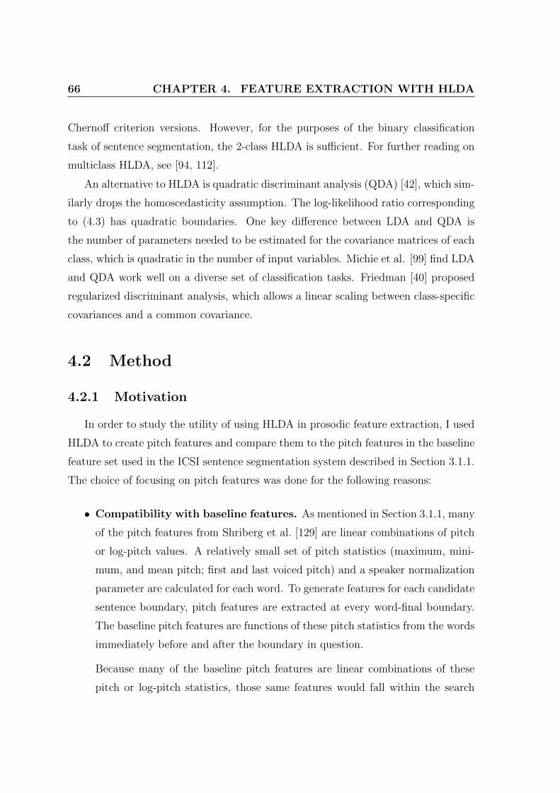
66 CHAPTER 4. FEATURE EXTRACTION WITH HLDA
Chernoff criterion versions. However, for the purposes of the binary classification
task of sentence segmentation, the 2-class HLDA is sufficient. For further reading on
multiclass HLDA, see [94, 112].
An alternative to HLDA is quadratic discriminant analysis (QDA) [42], which sim-
ilarly drops the homoscedasticity assumption. The log-likelihood ratio corresponding
to (4.3) has quadratic boundaries. One key difference between LDA and QDA is
the number of parameters needed to be estimated for the covariance matrices of each
class, which is quadratic in the number of input variables. Michie et al. [99] find LDA
and QDA work well on a diverse set of classification tasks. Friedman [40] proposed
regularized discriminant analysis, which allows a linear scaling between class-specific
covariances and a common covariance.
4.2 Method
4.2.1 Motivation
In order to study the utility of using HLDA in prosodic feature extraction, I used
HLDA to create pitch features and compare them to the pitch features in the baseline
feature set used in the ICSI sentence segmentation system described in Section 3.1.1.
The choice of focusing on pitch features was done for the following reasons:
• Compatibility with baseline features. As mentioned in Section 3.1.1, many
of the pitch features from Shriberg et al. [129] are linear combinations of pitch
or log-pitch values. A relatively small set of pitch statistics (maximum, mini-
mum, and mean pitch; first and last voiced pitch) and a speaker normalization
parameter are calculated for each word. To generate features for each candidate
sentence boundary, pitch features are extracted at every word-final boundary.
The baseline pitch features are functions of these pitch statistics from the words
immediately before and after the boundary in question.
Because many of the baseline pitch features are linear combinations of these
pitch or log-pitch statistics, those same features would fall within the search

4.2. METHOD 67
space of a LDA/HLDA transformation. One may question why I choose to
attempt to duplicate the work of Shriberg. For example, the combination of
the baseline features and resulting HLDA features probably will not give much
improvement. However, the goal of this study is not purely performance driven,
but to test whether statistical learning methods can be used in the design of
prosodic features. Having some of the baseline pitch features within the search
space of the HLDA transform provides a reference point to judge whether the
HLDA system is successful or not.
• Interpretability. The HLDA produces a linear transformation on its input
pitch/log-pitch statistics that attempts to maximize the separation between
sentence and non-sentence boundary classes. This linear transformation is rel-
atively easy to interpret as we can examine which input statistics and what rel-
ative combination of input statistics are important. This may provide insight
into the further design of pitch features. For comparison, one might extract
classification features from the hidden layer of a multilayer perceptron (MLP),
a popular non-linear classifier. How the MLP transforms the input data is
relatively opaque compared to the simple linear combination of LDA/HLDA.
• Language-independent system. As mentioned in Section 3.3.3, we believe
that the baseline pitch features originally designed for English are less well-
suited for tonal languages such as Mandarin because the lexical intonation bi-
ases the pitch statistics used in feature extraction. One intention in focusing
on this known problem is to see whether the HLDA system can learn to com-
pensate for idiosyncracies in the target language. If so, then this could save the
researchers considerable effort of having to redesign prosodic features themselves
when porting between different languages and domains.
4.2.2 System
The only change from the baseline system in Section 3.2 is that the HLDA system
replaces the original feature extraction step (see Figure 4.2). Both systems use the

68 CHAPTER 4. FEATURE EXTRACTION WITH HLDA
Figure 4.2: Block diagram of the HLDA feature extraction system compared to base-line system. Both share the same pitch statistics and classifier. Feature selection onHLDA features is optional.
same pitch statistics and LTM speaker parameters and classifier. In this way, we can
directly compare the HLDA system to the baseline pitch feature designs.
The HLDA is trained on the training data, ideally finding a linear transforma-
tion that will maximize the separation between the class feature distributions. This
transformation is applied to the train, dev, and eval sets. As before, the AdaBoost
classifier model is trained on the train set, a posterior probability threshold is calcu-
lated using the dev, and the held-out eval is used for performance evaluation. What
needs to be determined are the various settings in the implementation of the HLDA,
which are described below.
The data sets were set up as in Section 3.2.3, with data split 80/10/10% between
train, dev, and eval sets, respectively. In this chapter, I only used the English
corpus, as the baseline feature were originally designed for English and that is the
language with the most data.
4.2.3 HLDA parameters
The following describes different settings in how the HLDA system is set up.

4.2. METHOD 69
Raw statistics vs. HLDA
To test whether the HLDA transformation leads to any improvement in perfor-
mance, some experiments were performed with HLDA disabled. That is to say the
input pitch statistics pass through unmodified and are used directly as the feature
vectors by the AdaBoost learning algorithm. For this dissertation, I will use the fol-
lowing notation to differentiate between these experiments: stat denotes trials where
HLDA is disabled, and hlda will denote when it is enabled.
The missing value handling setting described below is not relevant to the stat ex-
periments, so they do not use that parameter. stat experiments are still labeled with
the size of context and pitch-domain parameters according to their settings. The hlda
is labeled with all three parameters. For example, stat 2W log denotes the log-pitch
statistics from the 2-word context without the HLDA transform, and hlda 4W pitch
corresponds to the HLDA features transformed from the non-log pitch statistics from
the 4-word context.
Size of context
To calculate classification features for each candidate boundary, the baseline set
of pitch features limit themselves to being functions of pitch statistics from only the
words immediately before and after the boundary for simplicity and computational
constraints. As mentioned in the Compatibility with Baseline Features bullet in
Section 4.2.1, one objective of testing the HLDA feature extraction is to compare
it to the baseline set of polished human-design features. To make this comparison
as close as possible, for one set of experiments, the pitch statistics used as HLDA
input are similarly limited to the words before and after the word-final boundary in
question. These are referred to as the 2-word (2W) context experiments.
The input to HLDA is a supervector containing the pitch statistics from these
words from the context. Under this construction, it is simple to expand the context
used by the HLDA transformation by appending pitch statistics from more words.
The experiments below tested a 4-word (4W) context, using pitch statistics from the
two words before and the two after the candidate boundary, though larger contexts

70 CHAPTER 4. FEATURE EXTRACTION WITH HLDA
Figure 4.3: Illustration of 2-word and 4-word context. The input to the HLDAtransform is comprised of the five pitch statistics extracted over each word in thecontext, plus the speaker LTM parameter(s).
can also be tested. See Figure 4.3.
It should be noted that, because the context is based on words, the amount of
time and therefore the number of acoustic frames used to calculate each feature can
vary greatly, and one may expect greater pitch variation over longer windows, which
would be reflected in the pitch statistics. Alternatives to words include counting by
syllables, which are of more consistent duration than words, or trying to capture
suprasegmental behavior over a fixed window surrounding the word-final boundary.
However, as stated, to keep the HLDA-generated features comparable to the baseline
pitch features, I chose to control the amount of context as described above.
Pitch domain
As it is not clear whether it is pitch ratio or absolute pitch difference that cues
sentence boundaries, three options were tested for which pitch values to use as the
input to the HLDA transformation:
• Pitch: absolute pitch values.
• Log-pitch: log of the above pitch values.

4.2. METHOD 71
• Both: both pitch and log-pitch values are concatenated, making the input su-
pervector to the HLDA transformation twice as long. Note that this is different
from concatenating the pitch and log-pitch HLDA features.
In the case of absolute pitch and log-pitch, each word contributes its five pitch
statistics — maximum, minimum, mean, and first and last voiced pitch — calculated
as described in Section 3.1.1. Including both absolute pitch and log-pitch values
allows the HLDA transformation to compute features that examine both absolute
pitch values and pitch ratios. However, it is difficult to interpret an HLDA feature
that mixes absolute pitch and log-pitch values of the same statistic, let alone different
statistics. There is also the issue that absolute pitch and log-pitch values will be
highly correlated, which may lead to the matrices involved in the HLDA transform
to appear to have less than full rank.
To create the HLDA input, in addition to the five pitch statistics from each word
in the context, speaker normalization is achieved by including a speaker parameter
from the word immediately before the word-final boundary. Again, to keep the HLDA
features as close as possible to the baseline pitch features, the speaker parameter is the
same one used by the baseline feature set, the lognormal tied mixture (LTM) model
speaker baseline parameter [138]. This speaker parameter is either in absolute pitch,
log-pitch, or both according to the pitch domain parameter. Although different words
within the context may come from different speakers, and thus ideally have their own
speaker normalization parameter, for most word-final boundaries all the words come
from the same speaker, and thus all of the speaker parameters would be exactly the
same. This near singularity may be problematic for the HLDA transform, so only
the speaker parameter of the word immediately before the boundary in question is
included in the HLDA input supervector.
The combination of size of context and pitch domain parameters determines the
size of the HLDA input supervector, and therefore the number of output features as
well. The smallest number of features tested is 11: 5 pitch or log-pitch values from
each word in a 2-word context plus the LTM speaker baseline parameter. The largest

72 CHAPTER 4. FEATURE EXTRACTION WITH HLDA
number of features tested is 42: 5 absolute pitch values from a 4-word context plus
the LTM parameter gives 21 inputs; adding the log-pitch versions of the same doubles
the total to 42.
Treatment of missing data
In the cases where no voiced pitch is found within a word boundary, the algorithm
has no valid pitch values to operate on and so returns a missing value in all pitch
statistics for that word. This generally only happens in short words and when the
pitch tracker has trouble finding the fundamental frequency of the voiced speech,
thus the pitch values would be less reliable. Missing pitch values occured in 1.12%
of the words of the TDT4-ENG corpus. Even in the absence of this information, the
classification algorithm still must make a decision.
This parameter controls how the HLDA system treats missing values in the train-
ing data only; treatment of missing data during classification is described further
down. Words with missing pitch values are handled in one of two ways:
• Drop: These words are considered suspect since there must be some acoustic
reason that no voiced pitch was detected. All supervectors that would contain
missing values (i.e. any context which includes such words) are therefore re-
moved from the training data. The idea is to clean up the training data so a
good HLDA transform can be trained.
• Mean fill: In comparison, the reasoning here is to make the training data re-
semble the data during classification. In the aforementioned system description,
HLDA must still classify words with missing pitch values, and so those words are
mean filled. Therefore missing values in the training data are similarly mean-
filled in hopes that the resulting HLDA transformation learns to compensate
accordingly.
A more thorough treatment of missing values would examine whether the fact
that the word is missing data is useful information [91, 117]. The baseline feature set
propogates missing data by labeling the features that depend on missing data to also
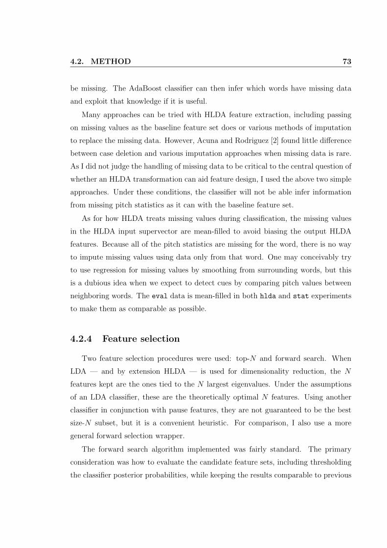
4.2. METHOD 73
be missing. The AdaBoost classifier can then infer which words have missing data
and exploit that knowledge if it is useful.
Many approaches can be tried with HLDA feature extraction, including passing
on missing values as the baseline feature set does or various methods of imputation
to replace the missing data. However, Acuna and Rodriguez [2] found little difference
between case deletion and various imputation approaches when missing data is rare.
As I did not judge the handling of missing data to be critical to the central question of
whether an HLDA transformation can aid feature design, I used the above two simple
approaches. Under these conditions, the classifier will not be able infer information
from missing pitch statistics as it can with the baseline feature set.
As for how HLDA treats missing values during classification, the missing values
in the HLDA input supervector are mean-filled to avoid biasing the output HLDA
features. Because all of the pitch statistics are missing for the word, there is no way
to impute missing values using data only from that word. One may conceivably try
to use regression for missing values by smoothing from surrounding words, but this
is a dubious idea when we expect to detect cues by comparing pitch values between
neighboring words. The eval data is mean-filled in both hlda and stat experiments
to make them as comparable as possible.
4.2.4 Feature selection
Two feature selection procedures were used: top-N and forward search. When
LDA — and by extension HLDA — is used for dimensionality reduction, the N
features kept are the ones tied to the N largest eigenvalues. Under the assumptions
of an LDA classifier, these are the theoretically optimal N features. Using another
classifier in conjunction with pause features, they are not guaranteed to be the best
size-N subset, but it is a convenient heuristic. For comparison, I also use a more
general forward selection wrapper.
The forward search algorithm implemented was fairly standard. The primary
consideration was how to evaluate the candidate feature sets, including thresholding
the classifier posterior probabilities, while keeping the results comparable to previous

74 CHAPTER 4. FEATURE EXTRACTION WITH HLDA
experiments. Each iteration, the dev set is randomly split in half. One half is used
to train the threshold, the other half is used for evaluation, and the greedy forward
search is based on these results. By using a different random split in each iteration,
the algorithm avoids biasing feature selection toward any particular portion of the
dev set while the training set is kept the same as previously described experiments.
In order to compare the candidate feature sets to earlier experiments, a threshold was
trained on the full dev set and evaluated on the held-out eval set, but these results
were not used by the feature selection algorithm. The modified forward selection
algorithm is shown below.
• Initialize feature set F with the four pause features and P with pitch features
from HLDA.
• While P is non-empty: let t be the current iteration index
1. Randomly split dev set D into DtT and DtE
2. For each feature pi ∈ P :
(a) Create candidate feature set Ci = {F , pi}
(b) Train classifier model Mi using features Ci on training data T .
(c) Evaluate the classifier Mi on DtE using threshold trained on DtT .
3. Find the best performing feature set Ci, remove pi from P and add to F .
Forward selection algorithm, detailing which feature sets
are used for thresholding and evaluation
Stopping criterion. Starting with M features, the two feature selection methods
produce a sequence of features sets with sizes ranging from 1 to M features. Generally
feature selection experiments are allowed to terminate before reaching the full feature
set if it is clear there will be no further improvement, but there was no clear indicator
for that here. Indeed, for the English HLDA features, the best stopping point often
included most of the feature set.
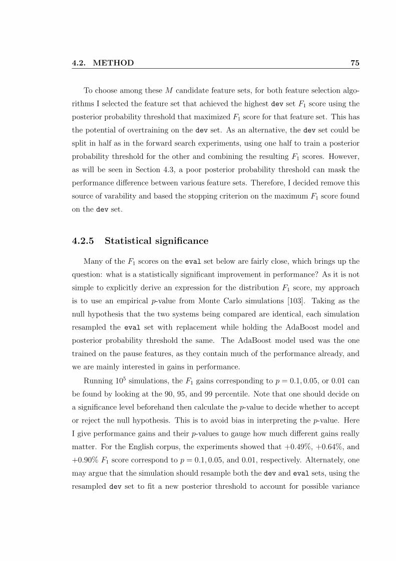
4.2. METHOD 75
To choose among these M candidate feature sets, for both feature selection algo-
rithms I selected the feature set that achieved the highest dev set F1 score using the
posterior probability threshold that maximized F1 score for that feature set. This has
the potential of overtraining on the dev set. As an alternative, the dev set could be
split in half as in the forward search experiments, using one half to train a posterior
probability threshold for the other and combining the resulting F1 scores. However,
as will be seen in Section 4.3, a poor posterior probability threshold can mask the
performance difference between various feature sets. Therefore, I decided remove this
source of varability and based the stopping criterion on the maximum F1 score found
on the dev set.
4.2.5 Statistical significance
Many of the F1 scores on the eval set below are fairly close, which brings up the
question: what is a statistically significant improvement in performance? As it is not
simple to explicitly derive an expression for the distribution F1 score, my approach
is to use an empirical p-value from Monte Carlo simulations [103]. Taking as the
null hypothesis that the two systems being compared are identical, each simulation
resampled the eval set with replacement while holding the AdaBoost model and
posterior probability threshold the same. The AdaBoost model used was the one
trained on the pause features, as they contain much of the performance already, and
we are mainly interested in gains in performance.
Running 105 simulations, the F1 gains corresponding to p = 0.1, 0.05, or 0.01 can
be found by looking at the 90, 95, and 99 percentile. Note that one should decide on
a significance level beforehand then calculate the p-value to decide whether to accept
or reject the null hypothesis. This is to avoid bias in interpreting the p-value. Here
I give performance gains and their p-values to gauge how much different gains really
matter. For the English corpus, the experiments showed that +0.49%, +0.64%, and
+0.90% F1 score correspond to p = 0.1, 0.05, and 0.01, respectively. Alternately, one
may argue that the simulation should resample both the dev and eval sets, using the
resampled dev set to fit a new posterior threshold to account for possible variance

76 CHAPTER 4. FEATURE EXTRACTION WITH HLDA
there. This would likely increase the performance gains necessary for the different
empirical p-value levels.
4.3 Results and Analysis
It was expected that increasing the size of the context would improve performance
at least slightly. As for pitch domain and treatment of missing values, there are
arguments in favor of each option. As nothing in these settings appear mutually
exclusive, all possible combinations of HLDA system settings were tried.
4.3.1 2-word context
Table 4.1 compares the performance of the pre-HLDA pitch statistics using only
a 2-word context to various baseline feature sets. From Chapter 3, recall that we
found F1 score to be a more reliable and stable evaluation measure than NIST error
for system development, even if NIST error is the measure ultimately used in system
evaluations. For this reason, in this chapter and the next, my analysis will focus on
the F1 score, though NIST error results will be included for general interest.
The type of feature type most useful for establishing a baseline is the four pause
features (PAU). Feature PAU DUR is the duration of the pause at the candidate bound-
ary in question. This is by far the best single predictor of a sentence boundary as a
long pause is highly indicative of a sentence boundary. The other features are shifted
versions of the same pause duration from the two word-final boundaries before and
the one boundary immediately after the boundary in question. Although the Ad-
aBoost algorithm using single node CART trees for weaker learners makes it harder
to explicitly learn from feature interaction — for example, moderate pause may or
may not signal a sentence boundary depending on how long the previous inter-word
pause was — long pauses in the vicinity of the current word-final boundary will lower
the likelihood of the current boundary being a sentence boundary.
As can be seen in Table 4.1, almost all of the system performance comes from these
four features. Therefore it is pointless to discuss sentence segmentation features in

4.3. RESULTS AND ANALYSIS 77
the absence of pause features, and they are included in every feature set. In the
case of the HLDA system, the HLDA features are derived from the pitch statistics as
described in Section 4.2.3, and then PAU is appended to the resulting feature vector.
The HLDA algorithm does not have access to PAU features. Indeed, the distribution of
pause features, with the vast majority being duration zero and having a long one-sided
tail, is not a good match to the HLDA assumptions.
The other feature set for comparison is the baseline set of 29 pitch features used
in the ICSI sentence segmentation system plus the four pause features (ICSI), which
shows a 3.3% absolute improvement in F1 score over the pause features. Note that
these do not include the 200ms window pitch features or the pitch slope features. The
log-pitch statistics (stat 2W log) and pitch statistics (stat 2W pitch) yield most of
the performance gain. Furthermore, using both pitch and log-pitch statistics exceeds
the performance of the baseline pitch features. This is surprising as one would expect
the pitch and log-pitch statistics to have the exact same information content. Looking
at the oracle eval numbers, where the optimal likelihood threshold is used instead of
the threshold trained on dev data, we see this is somewhat misleading as ICSI suffers
slightly more than the other feature sets shown from suboptimal thresholding. Based
on the relative performance of the stat and ICSI feature sets, we may conclude that
a large part of feature design is the selection of the information sources — in this case,
capturing pitch contour behavior in the form of these pitch statistics — though how
these information sources are processed to create features can significantly contribute
to classifier performance.
Table 4.2 shows how these AdaBoost F1 scores changes when the HLDA transform
is applied to the above pitch statistics, with the two columns of hlda representing
the two methods I tested for the treatment of missing data. With the exception
of dropping missing values during training (hlda-Drop) on both pitch and log-pitch
statistics, the hlda feature sets all performed within 0.12% F1 score of each other. It
appears this outlier was due to poor thresholding, as can be seen in Table 4.3, which
shows performance using oracle thresholds for the same feature sets. The oracle
hlda results are also clustered fairly close together. This brings up the question,
given the disparity between the performance of the stat feature sets, of why all the

78 CHAPTER 4. FEATURE EXTRACTION WITH HLDA
FeaturesF1 score (%) NIST (%)
dev eval eval (oracle) evalPAU 62.66 62.38 62.38 81.08ICSI 66.53 65.70 65.86 67.37stat 2W pitch 65.67 64.63 64.85 72.84stat 2W log 66.73 65.09 65.18 72.05stat 2W both 67.54 65.93 66.00 69.39
Table 4.1: Performance of English pitch statistics from 2-word context without HLDAtransform relative to pause and baseline pitch feature sets. The three statistics featuresets are pitch, log-pitch, and their concatenation (both). Eval columns use the poste-rior threshold trained on the dev set while oracle uses the threshold that maximizesF1 score on the eval set.
hlda features performed so similarly. I will address this question in Section 4.3.4.
Statistics stat hlda-Drop hlda-MeanFillPitch 64.63 65.19 65.11Log-pitch 65.09 65.23 65.15Both 65.93 64.95 65.20PAU 62.38ICSI 65.70
Table 4.2: F1 scores of English HLDA feature sets from 2-word context relative to thepitch statistics sets they were computed from: pitch, log-pitch, or their concatenation(both). The stat column gives the performance of the statistics without HLDA. Thetwo HLDA columns indicate the method of handling missing data. The F1 scores forthe pause and baseline pitch features are provided for comparison.
There does not appear to be much difference between dropping or mean filling
missing data. Given the relative rarity of missing pitch values in this corpus, it prob-
ably should not be too surprising that it does not matter much how we deal with it.
There is a slight preference for the pitch and log-pitch feature sets to prefer drop-
ping missing values while the feature using both prefers mean filling. The difference
appears to be small enough that it can be dwarfed by other issues, such as poste-
rior thresholding and the selection of information sources, but the pattern appear to
continue in other experiments, so it is worth noting.
The performance gained by the HLDA process is only about a third of the gap
between stat and the ICSI baseline features. This implies that, while HLDA con-

4.3. RESULTS AND ANALYSIS 79
Statistics stat hlda-Drop hlda-MeanFillPitch 64.85 65.22 65.13Log-pitch 65.18 65.29 65.18Both 66.00 65.15 65.24PAU 62.38ICSI 65.86
Table 4.3: Oracle F1 scores of English HLDA feature sets from 2-word context rel-ative to the pitch statistics sets they were computed from: pitch, log-pitch, or theirconcatenation (both). Oracle uses the posterior threshold that maximizes the eval
F1 score for that feature set. The stat column gives the performance of the statisticswithout HLDA. The two HLDA columns indicate the method of handling missingdata. The oracle F1 scores for the pause and baseline pitch features are provided forcomparison.
sistently makes a significant improvement over using the raw pitch statistics, it does
not fully capture the classification ability of an expert-designed set of features. Fur-
thermore, the HLDA transform reduced the performance compared to both the raw
pitch and log-pitch statistics.
4.3.2 4-word context
Table 4.4 shows performance numbers corresponding to Table 4.1, comparing the
raw statistics and baseline feature sets, except using the 4-word context where statis-
tics from the two words before and two words after the boundary are used as inputs.
We again see that the log-pitch does slightly better than pitch statistics, and together
they outstrip either one individually by more than a full percentage point absolute.
Furthermore, there is a significant performance gain relative to 2-word context
results, which indicates that there is information relevant to the classification task to
be found from this wider context, even when presented with no processing past the
pitch statistics. Shriberg et al. when designing the ICSI pitch features, constrained
the features to pitch statistics drawn from the two words immediately surrounding the
boundary [129]. Various combinations of pitch statistics and normalizations from this
limited context produced 45 features: 29 using the same pitch statistics over words
HLDA is using; 12 similar ones using statistics over 200ms windows; and 4 pitch slope

80 CHAPTER 4. FEATURE EXTRACTION WITH HLDA
features using the piecewise linear stylization. There would be exponentially many
more combinations to consider when using a wider context, many of which will be
useless, but this creates a practical limit to how much complexity even an expert
human with considerable in-domain knowledge can handle in feature design. This
again motivates the question of how computers can be used in the feature design
process.
FeaturesF1 score (%) NIST (%)
dev eval eval (oracle) evalPAU 62.66 62.38 62.38 81.08ICSI 66.53 65.70 65.86 67.37stat 4W pitch 66.64 65.25 65.44 71.23stat 4W log 67.30 65.46 65.83 69.78stat 4W both 68.42 66.54 66.58 67.88
Table 4.4: Performance of English pitch statistics from 4-word context without HLDAtransform relative to pause and baseline pitch feature sets. The three statistics featuresets are pitch, log-pitch, and their concatenation (both). Eval columns use the poste-rior threshold trained on the dev set while oracle uses the threshold that maximizesF1 score on the eval set.
Tables 4.5 and 4.6 likewise are counterparts to Tables 4.2 and 4.3, showing how
F1 score changes when the HLDA is applied to the raw pitch statistics, both using
dev-trained and oracle likelihoods thresholds. As before, comparing both the oracle
and non-cheating results is important as the performance gains for different pitch
feature sets can be masked by suboptimal thresholding. As with the 2-word context,
the best performing feature set from among these comes from using both pitch and
log-pitch features, which even exceeds the oracle baseline F1 score of 65.86%, but it
is the only HLDA feature set to do so.
While the 4-word HLDA feature sets perform better than the 2-word HLDA fea-
ture sets, the performance gained by the HLDA transform here is smaller than the
performance gained in the 2-word context. This could be because, since the 4-word
stat feature sets have better performance, it is harder for the processing done by
HLDA to improve upon it.
As with the 2-word context, the HLDA experiments achieved similar performance,

4.3. RESULTS AND ANALYSIS 81
Statistics stat hlda-Drop hlda-MeanFillPitch 65.25 65.64 65.24Log-pitch 65.46 65.59 65.56Both 66.54 65.52 65.93PAU 62.38ICSI 65.70
Table 4.5: F1 scores of English HLDA feature sets from 4-word context relative to thepitch statistics sets they were computed from: pitch, log-pitch, or their concatenation(both). The stat column gives the performance of the statistics without HLDA. Thetwo HLDA columns indicate the method of handling missing data. The F1 scores forthe pause and baseline pitch features are provided for comparison.
Statistics stat hlda-Drop hlda-MeanFillPitch 65.44 65.74 65.56Log-pitch 65.83 65.85 65.68Both 66.58 65.71 66.08PAU 62.38ICSI 65.86
Table 4.6: Oracle F1 scores of English HLDA feature sets from 4-word context rel-ative to the pitch statistics sets they were computed from: pitch, log-pitch, or theirconcatenation (both). Oracle uses the posterior threshold that maximizes the eval
F1 score for that feature set. The stat column gives the performance of the statisticswithout HLDA. The two HLDA columns indicate the method of handling missingdata. The oracle F1 scores for the pause and baseline pitch features are provided forcomparison.
with the lowest F1 score partly attributed to suboptimal likelihood thresholding. As
mentioned above, it appears the pitch and log-pitch set prefer dropping missing values
while their combination prefers mean-filling. It should be noted that the treatment of
missing data is of greater importance here than in the 2-word context case since every
word with missing data now appears in the supervector of four boundaries instead of
two, and deleting missing values would remove all four of these boundaries from the
training data.

82 CHAPTER 4. FEATURE EXTRACTION WITH HLDA
Figure 4.4: Log of the HLDA eigenvalues for English HLDA features from 4-wordcontext and both pitch and log-pitch statistics. Note the sharp drop off at the endoccurs in HLDA feature sets using both pitch and log-pitch statistics due to highlycorrelated inputs.
4.3.3 Feature selection experiments
Top-N
Figure 4.4 shows the log eigenvalues of the HLDA transform for the 4-word context,
both pitch and log-pitch, mean fill feature set. Note that the eigenvalues decrease
at a steady rate, though slightly more quickly for the first few indices. The very
sharp drop at the end is common in feature sets that use both pitch and log-pitch
statistics as inputs, most likely due to the pitch and log-pitch statistics being highly
correlated. For comparision, Figure 4.5 shows the eigenvalues for 4-word context,
log-pitch only, drop missing values feature set. The 2-word context eigenvalues follow
a similar pattern. The main conclusion to be drawn from the eigenvalues is there
does not appear to be a clear point at which the features become distinctly worse to
help us choose a stopping point.

4.3. RESULTS AND ANALYSIS 83
Figure 4.5: Log of the HLDA eigenvalues for English HLDA features from 4-wordcontext and only log-pitch statistics. Compared to Figure 4.4, there is no sharp dropoff at the end.

84 CHAPTER 4. FEATURE EXTRACTION WITH HLDA
Table 4.7 shows the results of the N -best experiments for the 2-word context.
Note that Oracle-N refers to using the stopping point with the highest eval F1 score;
none of the scores in the table use oracle posterior thresholds. Firstly, according
to the oracle-N selection criterion, the best stopping point generally includes all or
almost all of the HLDA features. This implies many of the HLDA features provide
some additional discriminative ability.
Secondly, basing the selection criterion on the dev set F1 comes pretty close to the
oracle-N selection criterion, often hitting it exactly. Even when it is slightly off, the
performance gap is fairly small. Given that the optimal selection criterion chooses
almost all of the features, it is not surprising that the Top-N F1 scores are very close
to the results from the full feature sets, and thus still fall short of the baseline pitch
features.
Feature setAll HLDA features dev-N oracle-N
eval eval N eval NPitch-Drop 65.19 65.30 10 65.30 10Pitch-MeanFill 65.11 64.93 10 65.11 11LogPitch-Drop 65.23 65.23 11 65.23 11LogPitch-MeanFill 65.15 65.14 9 65.16 10Both-Drop 64.95 65.06 21 65.12 19Both-MeanFill 65.20 65.20 22 65.20 22
Table 4.7: F1 scores of Top-N feature selection experiments for English 2-word contextHLDA features. dev-N and oracle-N refer to different stopping criteria, where Ngives the size of the selected feature set. eval gives the corresponding F1 score of theeval set. dev-N is based off the dev set scores while oracle-N chooses the N withmaximum eval.
Table 4.8 shows the same Top-N numbers for the 4-word context case. In contrast
to the 2-word context condition, looking at the Oracle-N results, there is room for
feature selection to make a small improvement. However, using the dev set F1 scores
as the selection criterion appears to be less reliable than in the 2-word case. As can
be seen in Figure 4.6, the dev set F1 scores plateau around N = 10 or 11 while the
eval scores continue to rise slightly. In both of the non-log pitch statistics feature
sets, the highest peak of their dev F1 scores happened to come at the start of the

4.3. RESULTS AND ANALYSIS 85
plateau rather than later. Compare this to Figure 4.7. In both of these experiments,
the choices of N that would improve upon the performance of the feature set before
feature selection would be N ≥ 16 or 17. In light of this, the selection criterion for
English feature sets may be improved by penalizing small feature sets or finding a
more reliable stopping criterion.
Feature setAll features dev-N oracle-N
eval eval N eval NPitch-Drop 65.64 65.40 11 65.64 21Pitch-MeanFill 65.24 65.17 11 65.51 18LogPitch-Drop 65.59 65.72 18 65.81 20LogPitch-MeanFill 65.56 65.57 18 65.63 17Both-Drop 65.52 65.51 40 65.98 30Both-MeanFill 65.93 65.84 40 65.96 38
Table 4.8: F1 scores of Top-N feature selection experiments for English 4-word contextHLDA features. dev-N and oracle-N refer to different stopping criteria, where Ngives the size of the selected feature set. eval gives the corresponding F1 score of theeval set. dev-N is based off the dev set scores while oracle-N chooses the N withmaximum eval.
Despite this difficulty in selection criterion, two of the Top-N feature sets can
match the performance of the baseline pitch features, and a third could have too
with a more fortunate stopping point. This shows that, by being able to process
more information, a fully automated feature design system can be competitive with
an expert-designed set of features.
Forward search
Table 4.9 shows the results of the forward search experiments for the 2-word
context. As with the Top-N experiments, none of these F1 scores use oracle thresh-
olding on posterior probabilities. Looking at the oracle-N results, a forward search
algorithm can usually give a slight performance gain, more so than the comparable
Top-N experiments in Table 4.7. Like the Top-N experiments, we see that for the
2-word context the best feature subset will still contain most of the HLDA features.
Examining the order in which HLDA features are selected in these experiments

86 CHAPTER 4. FEATURE EXTRACTION WITH HLDA
Figure 4.6: F1 scores on dev and eval sets versus N for Top-N feature sets from En-glish 4-word context HLDA features from pitch statistics using mean fill. dev scoresplateau around N=11 while eval continues to slowly increase. An early peak indev score results in a relatively poor eval score.
Figure 4.7: F1 scores on dev and eval sets versus N for Top-N feature sets fromEnglish 4-word context HLDA features from log-pitch statistics dropping missingdata. dev scores plateau around N=11 while eval continues to slowly increase. Anlate peak in dev score results in a relatively good eval score.
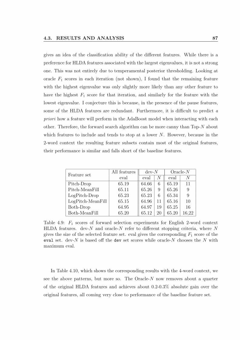
4.3. RESULTS AND ANALYSIS 87
gives an idea of the classification ability of the different features. While there is a
preference for HLDA features associated with the largest eigenvalues, it is not a strong
one. This was not entirely due to temperamental posterior thresholding. Looking at
oracle F1 scores in each iteration (not shown), I found that the remaining feature
with the highest eigenvalue was only slightly more likely than any other feature to
have the highest F1 score for that iteration, and similarly for the feature with the
lowest eigenvalue. I conjecture this is because, in the presence of the pause features,
some of the HLDA features are redundant. Furthermore, it is difficult to predict a
priori how a feature will perform in the AdaBoost model when interacting with each
other. Therefore, the forward search algorithm can be more canny than Top-N about
which features to include and tends to stop at a lower N . However, because in the
2-word context the resulting feature subsets contain most of the original features,
their performance is similar and falls short of the baseline features.
Feature setAll features dev-N Oracle-N
eval eval N eval NPitch-Drop 65.19 64.66 6 65.19 11Pitch-MeanFill 65.11 65.26 9 65.26 9LogPitch-Drop 65.23 65.23 6 65.34 9LogPitch-MeanFill 65.15 64.96 11 65.16 10Both-Drop 64.95 64.97 19 65.25 16Both-MeanFill 65.20 65.12 20 65.20 16,22
Table 4.9: F1 scores of forward selection experiments for English 2-word contextHLDA features. dev-N and oracle-N refer to different stopping criteria, where Ngives the size of the selected feature set. eval gives the corresponding F1 score of theeval set. dev-N is based off the dev set scores while oracle-N chooses the N withmaximum eval.
In Table 4.10, which shows the corresponding results with the 4-word context, we
see the above patterns, but more so. The Oracle-N now removes about a quarter
of the original HLDA features and achieves about 0.2-0.3% absolute gain over the
original features, all coming very close to performance of the baseline feature set.

88 CHAPTER 4. FEATURE EXTRACTION WITH HLDA
Feature setAll features dev-N Oracle-N
eval eval N eval NPitch-Drop 65.64 65.66 15 65.76 17Pitch-MeanFill 65.24 65.69 14 65.77 15LogPitch-Drop 65.59 65.53 9 65.85 19LogPitch-MeanFill 65.56 65.55 20 65.72 11Both-Drop 65.52 65.46 21 65.87 38,39Both-MeanFill 65.93 65.50 25 65.93 42
Table 4.10: F1 scores of forward selection experiments for English 4-word contextHLDA features. dev-N and oracle-N refer to different stopping criteria, where Ngives the size of the selected feature set. eval gives the corresponding F1 score of theeval set. dev-N is based on the dev set scores while oracle-N chooses the N withmaximum eval.
4.3.4 Interpretation of HLDA features
A linear transform was chosen for this initial attempt at machine designed features
in hopes that it may shed light on feature design. Below are the first four HLDA
features from the 2-word context, non-log pitch features, dropping missing values
feature set. While the forward search AdaBoost wrapper did not strongly prefer
these features, with a linear classifier and in the absence of the pause features, these
are theoretically the linear combinations with the best discriminative ability. For each
feature, I have normalized the largest component to norm 1 and listed all terms with
coefficients with absolute value ≥ 0.25. A 2-class HLDA projects the data into feature
space where, for each feature, moving in one direction represents higher likelihood of
one class while moving in the other direction represents higher likelihood of the other
class. In these four features, they are presented so that higher values indicate a
greater likelihood of a sentence boundary, according to the AdaBoost model.
The first feature is fairly easy to interpret: it looks for a pitch reset across the
boundary by comparing the last pitch of the word before to the first pitch of the word
after. Here, a high p1 would indicate a sentence boundary. The next term accounts
for the mean of the previous word so that, if the mean is high, then a low last pitch
indicates a sharp drop toward the end.

4.3. RESULTS AND ANALYSIS 89
p1 =− PrevLast+ 0.84NextF irst+ 0.46PrevMean− 0.26PrevMin
+ 0.26NextMean
p2 =PrevMean− 0.42PrevMin− 0.35PrevMax− 0.30NextMean
p3 =NextMean− 0.73NextMin− 0.32NextF irst+ 0.29NextLast
p4 =− PrevMin+ 0.90PrevF irst+ 0.63PrevLast− 0.53PrevMean
As for the other features, it is difficult to determine what cues or what quantities
they are trying to measure. I consulted Dr. Shriberg [125], but it was not clear to
her how to interpret these features. Thus, while one motivation for using a linear
transform such as HLDA for this task was feature interpretability, it appears that
what insights we can draw from the results are limited.
The following compares the first HLDA feature for the pitch, log-pitch, and both
pitch + log-pitch feature sets for the 2-word context, dropping missing values from
the training data. Again, the largest coefficient has been normalized to unity, and
coefficients with magnitude smaller than 0.25 hidden. What we see explains why all of
the HLDA feature sets behave so similarly, even the experiments with both pitch and
log-pitch statistics that performed considerably better without the HLDA transform.
Even though the pitch and log-pitch statistics are highly correlated, AdaBoost was
able to exploit some non-redundant information. However, the HLDA transform
effectively reduced all different input statistics sets to the same features. This implies
that a different discriminant transform, preferably a non-linear one, may be better
suited for this task.
p1 =− PrevLast+ 0.84NextF irst+ 0.46PrevMean− 0.26PrevMin+ 0.26NextMean
l1 =− PrevLast+ 0.78NextF irst− 0.45PrevMean
b1 =− PrevLastLog + 0.60NextF irstLog − 0.44PrevMeanLog
+ 0.2 ∗ (−PrevLastPitch − 0.58NextF irstPitch − 0.45PrevMeanPitch)

90 CHAPTER 4. FEATURE EXTRACTION WITH HLDA
While analyzing the HLDA feature coefficients, I noticed that some statistics
tended to work together — that is, their coefficients usually have the same sign —
while others were in opposition. To capture this behavior, the correlations between
the statistic coefficients were calculated, the top five of which are shown in Table
4.11. Note that these are correlations, not correlation coefficients. Thus the Mean
statistics, which generally are strong components of the HLDA features, are well-
represented. My conjecture is that, of the five pitch statistics, the mean statistics are
the most robust because they are functions of the entire word region. Thus they are
useful measures of pitch height and for normalization.
Correlation Features-0.314 PrevMean PrevMin-0.263 NextMean NextMax+0.178 PrevMean NextFirst+0.158 PrevMean NextLast-0.157 PrevMean NextMin
Table 4.11: Largest correlations between HLDA feature coefficients.
4.4 Conclusion
These experiments set out to see whether machine learning methods could be
applied to the design of prosodic features. The benchmark for comparison was a
well-established set of features that has been used and refined in a variety of speech
processing tasks for over a decade. The HLDA features and the baseline features use
the same pre-processing steps up to and including the extraction of pitch statistics
over word intervals. From then on, the baseline features were hand-designed by a
human with expert knowledge to quantify various pitch levels and dynamics from
these pitch statistics. In the HLDA features, these pitch statistics were fed into
a discriminant transform to create linear combinations that would hopefully have
better classification power than the input statistics.
If we split feature design into selecting a source of information and processing of
that information into the features to be used by the learning algorithm, one clear mes-

4.4. CONCLUSION 91
sage from the above experiments is that the information source is important. When
the unprocessed pitch statistics were added to pause features, that already produced
much of the performance gain seen in the baseline pitch feature set. Furthermore,
when the contextual window was increased from the surrounding 2 words to a 4-word
context, performance was given a significant boost. Recall that, during the design
of the baseline pitch features, the features were intentionally limited to the statis-
tics drawn from the two words surrounding the boundary because, even under this
restriction, 45 pitch features were created. For a human to design features from a
wider context would soon become impractical. In contrast, computers are designed
to process large quantities of data, and with this additional contextual information
HLDA achieved performance comparable to the baseline pitch features.
One may argue that the pitch statistics used already have processed the pitch in-
formation to a large degree. Indeed, the motivation for the machine-designed features
is to make feature design accessible to researchers who do not already possess expert
knowledge in the conditions they are working on, say if a scientist whose background
is in English is tasked to design features for Mandarin or a system previously built
for broadcast news is ported to meetings data. In the creation of the pitch statistics,
someone chose to: remove halving/doubling pitch tracker errors with the lognormal
tied mixture model; smooth it with a median filter; extract long-term information
— at least longer than the typical 10ms frames — by using pitch statistics over
word-sized intervals; and to focus on five specific pitch statistics. Future work could
examine how well machine designed features perform if starting with less refined data,
such as syllable- or frame-level pitch values.
Of the various HLDA parameter settings explored, log-pitch statistics tend to
outperform absolute pitch, but they are very close. Furthermore, their combination
usually performs slightly better, but as not as much as one would expect if looking
at the performance of their corresponding pitch statistics sets, as will be discussed
below. As for the treatment of missing data, since these examples are relatively rare,
there is not much difference between dropping missing data or mean-filling. There is
a tendency for the pitch and log-pitch feature sets to prefer dropping missing data
and pitch + log-pitch to prefer mean-fill.

92 CHAPTER 4. FEATURE EXTRACTION WITH HLDA
Looking at the performance of the HLDA feature sets, we find that, at least when
starting with pitch or log-pitch statistics, the HLDA features perform slightly better
than the pitch statistics, but still closer to the pitch statistics than the baseline pitch
features. That implies the value added by the HLDA transform by itself is marginal
compared to that of Shriberg in the design of the baseline pitch features. There are
indications that HLDA is not a good choice for extracting features in this scenario.
The most prominent evidence is that, while the combination of pitch and log-pitch
statistics outperformed either separately, after each set was passed through HLDA,
their performance was similar, and the pitch + log-pitch statistics set dropped in
performance. This is attributed to the linear transform of the HLDA which, when
supplied with the highly correlated pitch and log-pitch statistics, extracted much the
same features. Future experiments should use a more general discriminant transform
or learning algorithm, ideally taking into consideration the classifier to be used and
the fact that the features will be used in conjunction with the pause features. Indeed,
for a while I experimented with multi-layer perceptrons, but the system performed
poorly and so the results are not included.
Because of the small performance differences between various feature sets, one
of the issues that plagued these experiments was the thresholding for the classifier
posterior probabilities. The posterior threshold trained on the dev set may provide
an F1 score on the held-out eval set close to theoretical maximum using the oracle
threshold, but often suboptimal thresholding may mask performance gains made by
the system, which is why I frequently referred to the oracle performance figures during
data analysis.
The feature selection experiments show that most of the HLDA features do have
discriminative ability as both the Top-N and forward search methods indicate that the
optimal feature subset should include most of the HLDA features. However, possibly
due to information redundancy in the presence of the pause features, the eigenvalues
of the HLDA features are not good indicators of whether to include the feature or not.
This is reminiscent of how filtering was not a strong predictor for the feature selection
experiments in Chapter 3. However, even these basic feature selection methods were
able to produce a small performance gain over the full HLDA feature sets. It should

4.4. CONCLUSION 93
be noted that the posterior probability thresholding issues mentioned above interfered
with the stopping criterion for the feature selection algorithms.

94
Chapter 5
Language Independence
One of the objectives of the proposed HLDA feature design system is to see
whether it can extract prosodic features for a new language or condition without
requiring considerable in-domain knowledge. A survey of sentence segmentation re-
search in languages other than English was presented in Section 2.2.4. Guz et al. [58]
addressed the agglutenative morphology of Turkish by creating morphological fea-
tures, especially targeting the subject-object-verb ordering that is common to Turkish
broadcast news. To make use of this information, they implemented a morpholog-
ical analyzer for feature extraction and a factored version of a hidden event model
to accomodate the new features. Results showed that the addition of morphological
information improved performance significantly.
In contrast, Batista et al. [7] used pitch and segmental duration features based off
of Shriberg et al. [129], but without tweaking the features or system much to acco-
modate known prosodic patterns in European Portuguese regarding stressed syllables
and segmental duration. The result was that the syllable pitch and energy features
and the segmental duration features contributed little to performance.
One takeaway point from this is that compensating for language-specific behavior
is non-trivial. In the above examples, with human-designed features, considerable
work went into making productive features. The objective for this chapter is to
examine whether the proposed HLDA system can compensate for a known issue, the
interference of Mandarin lexical pitch, without being explicitly programmed to. That

5.1. BACKGROUND 95
is, while the resulting HLDA features may not be language independent, I wish to
test the robustness of the algorithm.
5.1 Background
5.1.1 Tone languages
Arguably the greatest difficulty in designing pitch features for Mandarin comes
from the fact that it is a tone language. As discussed in Section 2.1, the pitch
component of prosody is used to communicate a variety of information, including
phrasing, focus, and emotion. However, in tone languages, pitch is also used to
convey lexical and/or grammatical information.
Mandarin is the most widely-spoken tone language in the world. In Mandarin,
tones are differentiated by their characteristic pitch contour. Each syllable carries
its own tone, and there are many minimal pairs — minimal sets may be a better
description, as the examples involve more than two words, but the term minimal
pair is the one used in linguistics literature — such as the commonly given syllable
“ma,” which can mean mother, hemp, horse, or to scold depending on whether Tone
1 through Tone 4 is used. Phonetically, these words have the same phonemes and
only differ in intonation. It should be noted that such minimal pairs are composed
of words with greatly different meanings and parts of speech. Thus, lexical tone is
separate from inflectional morphology, such as initial-stress-derived nouns in English
that can change a verb to a noun [61]. For example:
• Verb: “I wish to record the recital.”
• Noun: “I have a record of the recital.”
where the accent mark denotes the stressed syllabe in the word. Here, a superfix —
an affix that consists of a supersegmental rather than phonetic change — modifies
the original morpheme’s meaning from a verb to a related noun or adjective [122].
However, in the case of Mandarin, the words in the minimal pairs are quite different,
and the tone is therefore is an essential component of the lexeme.

96 CHAPTER 5. LANGUAGE INDEPENDENCE
Not all tonal languages behave like Mandarin. In the Bantu family of languages
of sub-Saharan Africa, as opposed to the pitch contours of Mandarin, tones are dis-
tinguished by the relative pitch level. Tones may be attributed to whole words, as
opposed to individual syllables in Mandarin, and tone may convey grammatical in-
formation, such as verb tense or determining whether a pronoun is first-person or
second-person [22].
In Somali, the current phonological theory is that every word consists of one or
more mora, with short vowels containing one mora while long vowels contain two
morae. Except for particles, one of the last two morae of each word is marked with
a high tone. Therefore, in long-vowels, a High-Low mora sequence is produced as a
falling tone while a Low-High sequence is transformed by a phonological process to
High-High and be realized as a high tone, though sometimes it surfaces as a rising tone.
All other vowels are realized with a low tone. Tones are used to mark grammatical
differences rather than lexical ones, such as between singular and plural or masculine
or feminine gender [69].
Tonality in Japanese is usually described as pitch accent: each word may have zero
or one downsteps. Pitch gradually rises before the down step, undergoes a sudden
drop between two mora, and tends to stay level or drop slowly for the remainder of
the word. For example:
• At the chopsticks: hashını, the first mora is high while the remainder are low.
• At the bridge: hashını, the accent is perceived on the second mora, which is
why the first mora is transcribed a.
• At the edge: hashinı is perceived to be accentless or sound flat.
Like most languages, Japanese also features a gradual drop in pitch over a phrase.
However, it appears much of this drop comes from downsteps. Thus, the rise in pitch
before each downstep may be the result of the speakers needing to reset their pitch
higher to keep the utterance within their pitch range [109].
From the above sample of tone languages, we can see there is a great variety in
the ways tone is expressed and used to convey lexical or grammatical information.
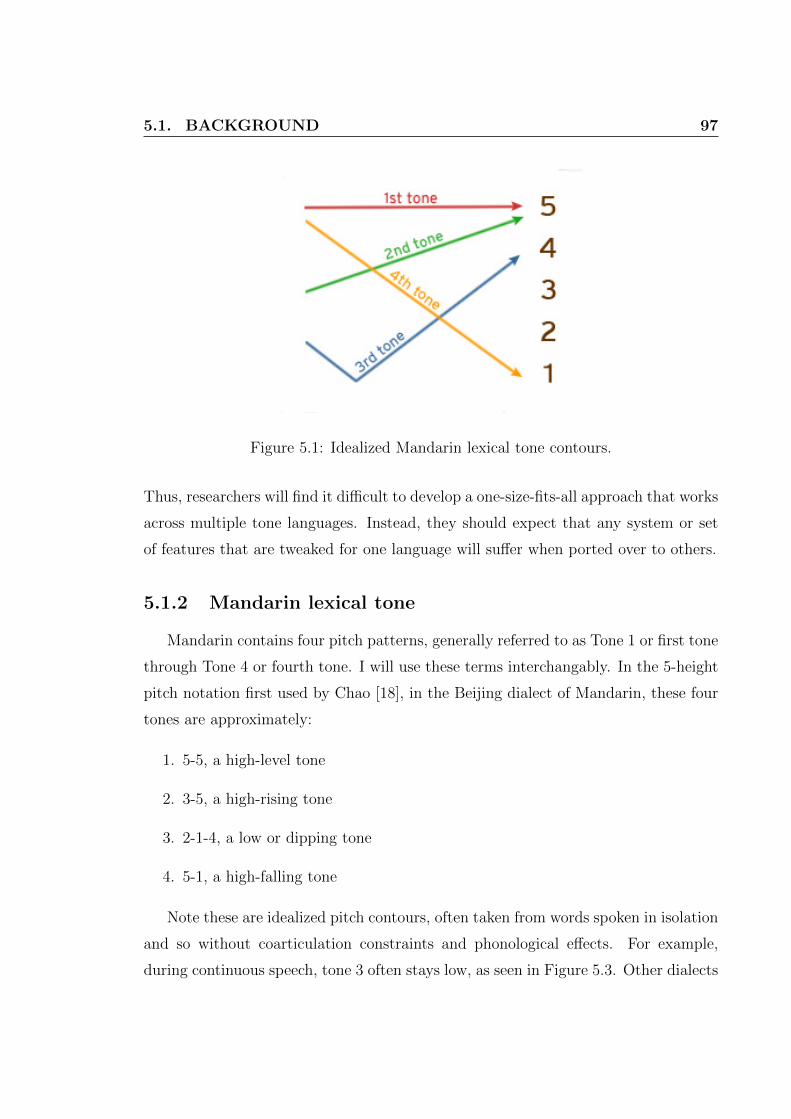
5.1. BACKGROUND 97
Figure 5.1: Idealized Mandarin lexical tone contours.
Thus, researchers will find it difficult to develop a one-size-fits-all approach that works
across multiple tone languages. Instead, they should expect that any system or set
of features that are tweaked for one language will suffer when ported over to others.
5.1.2 Mandarin lexical tone
Mandarin contains four pitch patterns, generally referred to as Tone 1 or first tone
through Tone 4 or fourth tone. I will use these terms interchangably. In the 5-height
pitch notation first used by Chao [18], in the Beijing dialect of Mandarin, these four
tones are approximately:
1. 5-5, a high-level tone
2. 3-5, a high-rising tone
3. 2-1-4, a low or dipping tone
4. 5-1, a high-falling tone
Note these are idealized pitch contours, often taken from words spoken in isolation
and so without coarticulation constraints and phonological effects. For example,
during continuous speech, tone 3 often stays low, as seen in Figure 5.3. Other dialects
98 CHAPTER 5. LANGUAGE INDEPENDENCE
of Mandarin have different pitch targets, though the general shape of the pitch contour
remains similar [19].
There is also a fifth tone, sometimes referred to as flat, light, or neutral tone, which
is pronounced as a light, short syllable. In contrast to the other tones, the fifth tone
has a relatively large number of allophones, with its pitch value greatly depending on
the tone of the syllable preceding it. Furthermore, while it usually appears at the end
of words or phrases, there is no fixed generative rule for when neutral tone occurs.
Phonologically, light tone may be viewed as a syllable with no underlying tone but
is realized at the surface by the spreading of the tone of the preceding syllable. In
any case, it is clear that fifth tone behaves fundamentally differently from the other
four tones and should be treated differently. In the TDT4-MAN corpus I used, fifth
tone was not used in the transcription, so the following experiments and analysis were
performed ignoring its existance.
The realization of Mandarin tone is further complicated by tone sandhi, which
may be thought of as phonological rules that alter lexical tones in certain contexts
[123]. Among tonal languages, there are other processes that may affect tone; for ex-
ample, in Cantonese, derivational morphology changes the low-falling tone of ‘dong’
meaning sugar, to the derived word ‘dong,’ candy, using a mid-rising tone [9]. How-
ever, Mandarin has relatively simple tone sandhi rules, mainly concerning the third
dipping tone, which is not surprising since, as the only tone that involves two pitch
changes, it is the most complex of the fundamental tones [19].
• When two consecutive third tones occur, the first one becomes a rising tone,
perceptively indistinguishable from second tone. The second syllable becomes
what is sometimes referred to as a half-third tone with pitch targets 2-1. For
example, ‘hen hao,’ very good, is pronouned ‘hen hao.’
• When more than two third tones occur in a row, this becomes further compli-
cated, and the exact surface realization also depends on the syllable-length of
the words involved.
• When the third tone is the first syllable of a multisyllable or compound word,
5.1. BACKGROUND 99
it is often reduced to a half-third tone during spontaneous speech. Examples of
this include ‘hao chi,’ good + eat = delicious ; ’hao kan,’ good + look = pretty.
• When two consecutive fourth tones occur, the first one does not fall so much
— it has been transcribed as pitch targets 5-3 — while the latter remains the
same. This makes the second syllable sound more emphatic. An example of
this is ‘zuoye,’ meaning homework.
• Two words — ‘yi,’ one, and ‘bu,’ no — have their own special rules. For
example, no takes on a second tone when followed by a fourth tone but becomes
neutral when coming between two words in a yes-no question. One should be
realized with Tone 1, 2, 4 or neutral, depending on the circumstances.
The presence of tone sandhi means that any pitch features that attempt to fully
quantify lexical tone should not rely on the dictionary lexical tone alone but take
into consideration both the surrounding tone environment and the lexical content of
the utterance. However, one of the desired aspects of prosodic features, as previously
mentioned, is for them to be computed and used in the absence of the lexical infor-
mation.
As has been discussed, the pitch contour produced is a function of many compet-
ing influences, including lexical tone, phrase declination, stress, and semantic focus.
However, as lexical tone carries information critical to the semantic content of the
speech, we would expect that it has a higher priority over other considerations, and
thus the pitch contour produced strongly reflects the syllable’s lexical tone. There-
fore, in the case of sentence segmentation and other applications of prosodic pitch, we
would expect lexical pitch to obscure the pitch contour cues and patterns we would
like to employ in these tasks. In Chapter 3, we indeed saw that the baseline ICSI
prosodic feature set had greater difficulty with Mandarin than English or Arabic,
especially its pitch features.
Therefore, to design a set of pitch features that is better able to handle the presence
of Mandarin lexical tones, one might want to study the interaction between lexical

100 CHAPTER 5. LANGUAGE INDEPENDENCE
tones and the sentence pitch contour. However, I have found little literature on this
topic. While there is a considerable body of work on the modeling of Mandarin lexical
tone, most of the research treats the interaction between syllables and sentence as an
additive or smoothing process between the two sources. Given this, it still behooves
us to study the current research into lexical tone modelling, as it will at least inform
us on how to compensate for the lexical tone.
Xu [170, 169, 174] argues that the fundamental representation of pitch contours
are pitch targets, which come in two varieties: static and dynamic. Static targets are
level and have a height — such as high, low, or mid — relative to the speaker’s pitch
range. Dynamic targets consist of a linear movement (in log-pitch domain).
There is a distinction between a dynamic pitch target being represented by a
line compared to a beginning and ending pitch target, which is the more traditional
representation from recent advancements in autosegmental and metrical phonology
[48, 49]. For example, a rising pitch contour may be represented by a low-high
sequence of pitch targets. Xu argues for the reality of these linear targets by observing
that the later portion of pitch contours converge on a target while the early portion
can vary greatly, generally due to the pitch trajectory of the previous lexical tone.
From this, he concludes that the pitch contour realized is one that asymptotically
and continuously approximates the pitch target. If a rising dynamic pitch target was
a sequence of low-high pitch targets, then one would expect the resulting pitch to
resemble the solid line in Figure 5.2 as pitch tries to converge to two pitch targets
in sequence. Instead, the pitch contour observed in rising tone syllables more closely
resembles the dotted line, which uses a sloping linear target.
The Stem-ML model of Kochanski, Shih, and Jing [75, 76, 77, 124] works under
the assumption that each lexical tone has an exemplar, an ideal tone shape that each
speaker implicitly knows. Stem-ML does not make any a priori assumptions as to
these tone shapes — such as pitch heights, lines, or targets — but instead learns them
from data. The resulting tone shapes, however, correspond well to the established
contours elsewhere in the literature. Note that while they refer to these templates as
tone shapes, it is not just the dynamics of the template that matters, but the absolute
pitch height as well.

5.1. BACKGROUND 101
Figure 5.2: Hypothetical pitch trajectories arguing for the existance of dynamic (slop-ing) pitch targets rather just high and low static targets from [170]. Figure (a) com-pares two potential targets, a rising dynamic target (dotted) and static high target(upper solid line). Starting from a low pitch, because pitch asymptotically approachestargets, the two hypothetical targets would produce the dashed and lower solid line,respectively. Similarly Figure (b) compares a rising dynamic target (dotted) to a se-quence of low-high static targets (outer solid lines). Again, these hypothetical targetswould produce the dashed and middle solid line, respectively. The dashed contoursare more natural, and so Xu concludes the existance of dynamic pitch targets.
The central idea behind the Stem-ML model is that the pitch contour produced
is a trade-off between effort, a quantity based on muscle dynamics where effort is
higher if muscles are moving faster or further from their neutral position, and error,
a measure of how much pitch deviates from the ideal tone template. Unlike Xu’s
framework, which places more weight on reaching the pitch target toward the end
of the syllable, the Stem-ML model uniformly weights pitch error over the span of
the pitch template. The trade-off between effort and error changes from syllable to
syllable, which they quantify using a prosodic strength parameter per syllable. If a
syllable’s prosodic strength is large, this represents the speaker’s willingness to expend
more energy to accurately produce the tone template and thus reduce communication
error, such as in careful speech. See Figure 5.3 from [76].
In fitting the prosodic strength parameters, the Stem-ML corroborates many find-
ings already present in the literature, including:
• Words follow a strong-weak metrical pattern [87].

102 CHAPTER 5. LANGUAGE INDEPENDENCE
Figure 5.3: Stem-ML tone templates (green) and realized pitch (red). In the first pairof syllables, the low ending of the 3rd tone and the high start of the 4th compromise toa pitch contour between them that also does not force the speaker to exert too mucheffort to change quickly. The speaker also manages to hit the template target for thebeginning of the first syllable and end of the last. In the second pair of syllables,the first syllable closely follows the tone template while the second syllable is shifteddownward.

5.1. BACKGROUND 103
• Words at the beginning of a sentence, clause, or phrase have greater strength
[65].
• Nouns and adverbs have greater strength than other parts of speech, and parti-
cles have the lowest. This reflects the low information content of function words
[64].
• There is a correlation between stress, which prosodic strength appears to be
related to, and duration [24, 74].
Their findings also suggest there is negative correlation between prosodic strength
and mutual information. That is, the easier it is to guess the current syllable from
previous ones — high mutual information — the lower its prosodic strength is since
it is less important to carefully pronounce the syllable to avoid confusion.
There is also ongoing debate as to what is the domain of tone. Given that the
pitch contour early in the syllable varies much more than the later portion, some [67]
conclude that the critical period for lexical tone is the syllable rhyme, the portion
of the syllable between the start of its nucleus and end of its coda, and the onset
serves as a transition period between tones. Kochanski and Shih allowed Stem-ML
to fit the span of the templates, which settled on approximately the last 70% of the
syllable. In the pitch target framework proposed by Xu, he defines the onset of the
pitch target as the time when the pitch contour begins to converge toward the target,
though he does not specify when exactly that occurs. When a falling tone follows high
or rising tone, i.e. tone that ends high, there is some delay before the pitch contour
begins to fall, so there is a period during the second syllable where pitch continues
to be high/rising. The Stem-ML model would predict such behavior as a result of
minimizing effort: pitch will continue to follow the trajectory of the previous tone
template and gradually transition to the following syllable’s template. In comparison,
when a low tone follows a high or rising tone, the pitch begins to decrease around the
syllable boundary. It should be noted that if there were no delay before pitch began
to lower during a falling tone, it would be hard to distinguish from a low tone, and
languages evolve to avoid such ambiguous situations.
104 CHAPTER 5. LANGUAGE INDEPENDENCE
On the note of a following syllable containing a pitch target with a low point,
i.e. third and fourth tone, Xu adds an additional rule to his proposed pitch target
framework to allow for anticipatory raising, which is a phenonmenon where the pitch
peak in such a situation is higher than it would be otherwise. Anticipatory raising
is sometimes called regressive H-raising or anticipatory dissimilation, and has been
observed in several tonal languages, including Enginni, Mankon, Kirimi [68], Thai
[46], Yoruba [84], and Mandarin [166]. In Xu’s pitch target framework, this pitch
peak is not a pitch target, but its occurence and location follow as a consequence of
implementing the pitch targets.
5.2 Method
The details about Mandarin lexical tone in Section 5.1.2 have numerous impli-
cations for the baseline ICSI pitch features and the proposed HLDA system. Recall
that these features are based on five pitch statistics — max, min, mean, and first and
last voiced pitch — over the word.
• Tone 1, which stays relatively high, will have high min and mean statistics.
• The last pitch will be heavily influenced by lexical tone of the word-final syllable.
• As the onset pitch of a syllable depends heavily on the final pitch of the preced-
ing syllable, the first pitch statistic depends on the lexical tone of the preceding
syllable. However, due to the way our system extracts pitch values, the corre-
lation will also depend on when voicing starts in the word-initial syllable. The
earlier voicing starts, the more the first pitch statistic will reflect the previous
syllable.
• Anticipatory raising will affect the max pitch of the preceeding and/or subse-
quent syllable, depending on when the pitch peak occurs.
Table 5.1 shows the mean and standard deviation of the five pitch statistics when
extracted over syllables instead of words, separating syllables by lexical tone. Some

5.2. METHOD 105
Tone 1 Tone 2 Tone 3 Tone 4 OverallStatistic µ σ µ σ µ σ µ σ µ σmax 233 73 209 69 199 69 227 75 219 73min 171 66 151 55 134 50 158 60 155 59mean 209 66 178 57 163 55 194 64 187 63first 186 70 184 70 189 67 191 71 188 70last 215 72 184 62 144 57 176 65 180 68
Table 5.1: Mean and standard deviation of pitch statistics for Mandarin syllables bylexical tone.
patterns are apparent in this table. Minimum and mean pitch have the lowest stan-
dard deviation, min probably because it is tied to the speaker baseline and mean
because it is a function of the entire syllable. The statistic with highest variance is
maximum pitch. Interestingly, all the µ — I will refer to the distribution mean as µ
to avoid confusion with the mean pitch statistic — of the first pitch are about the
same, around the level of the overall mean. This may be a reflection of onset pitch
depending on the preceding syllable. In contrast, the last pitch of tones 1 and 3 do
not seem constrained and go quite high and low, respectively.
To examine the coarticulation of pitch contours, especially at the beginning of the
syllables, Table 5.2 shows the mean and standard deviation of syllable pitch statistics
when conditioned on the tone of the previous syllable. As expected, the first pitch
of the syllable is the most affected, with it being particularly high after first tone
and low after third tone. Indeed, third tone appears to drag down all of the pitch
statistics of the following syllable. The other statistics are relatively unaffected by
the identity of the previous lexical tone, especially last pitch.
Table 5.3 compares the five pitch statistics of English and Mandarin when ex-
tracted over words. Again, min and mean have the lowest standard deviation. This
may explain why mean pitch was seen to be so commonly used by the HLDA system
in Section 4.3.4. Another thing to note is that, while it appears Mandarin has higher
standard deviation, it also has about twice the pitch range of English but not twice
the standard deviation.

106 CHAPTER 5. LANGUAGE INDEPENDENCE
Tone 1 Tone 2 Tone 3 Tone 4 OverallStatistic µ σ µ σ µ σ µ σ µ σmax 233 74 225 73 207 72 219 73 219 73min 167 63 162 59 138 53 152 58 155 59mean 199 65 193 63 176 59 183 63 187 63first 218 72 192 64 156 63 184 67 188 70last 181 68 184 69 181 66 177 69 180 68
Table 5.2: Mean and standard deviation of pitch statistics for Mandarin syllables bylexical tone of previous syllable.
English MandarinStatistic µ σ µ σmax 180 63 232 76min 132 46 139 53mean 156 49 185 59first 154 54 183 70last 150 54 183 70
Table 5.3: Mean and standard deviation of pitch statistics for English and Mandarinwords.
One method to compensate for lexical tone may be to model it and subtract it
away, leaving a pitch contour that more closely resembles the sentence intonation of
whatever pitch dynamics may be of interest. However, accurate lexical tone models
are not simple. Firstly, the underlying pitch target(s) for each tone must be defined
or calculated and, as noted in Section 5.1.2, even this fundamental issue is still under
debate.
Secondly, coarticulation causes the realized pitch contour to deviate from the tar-
get, and the degree of deviation varies within the syllable. Coarticulation is typically
handled by conditioning on the context surrounding the syllable in question. At a
minimum, this should be whether the previous syllable ended on a high or low pitch.
However, because the pitch trajectory of the preceeding syllable extends into the
following one, conditioning on the lexical tone of the previous syllable is warranted.
Thirdly, as Kochanski and Shih argue, the realization of lexical tone is not uniform
across all syllables, and prosodic strength depends on many factors, including the
position of the syllable within the word, the position of the word within the phrase or

5.2. METHOD 107
sentence, semantic focus, and how predictable it is given its context. In the sentence
segmentation task, we obviously do not know a priori the position of the word within
the sentence, though if prosodic strength can be calculated, it may help in inferring
its position within the sentence. Whether a word or syllable is predictable from its
context wanders into the territory of language models, and I wish to maintain the
independence of prosodic features if possible.
One of the motivations for proposing the use of machine learning techniques to
extract prosodic features is that designing a good set of features for a specific appli-
cation requires considerable domain knowledge, and even then feature design is not
a trivial process. Even if a good lexical model can be created, there is no guarantee
that it will greatly aid finding the sentence intonation that it obstructs.
To verify whether the proposed HLDA system can circumvent this requirement
of detailed in-domain knowledge, I repeated the experiments in Chapter 4 without
modification. Refer to Section 4.2.2 for a description of the system. The goal of
this chapter is to compare how the HLDA plus feature selection design process per-
forms here relative to English, and therefore whether the system can adapt to the
complications created by Mandarin lexical tone.
As an aside, the original inspiration for the proposed HLDA feature system was
the analysis of eigenpitch in Mandarin [146, 147], which performed a principal com-
ponent analysis (PCA) on Mandarin syllable intonation contours. The top principal
components found reflect the well-known Mandarin lexical pitch contours (see Figure
5.4). The context for this work was concatenative speech synthesis, where the desired
speech utterance is created by stringing together units selected from a pre-recorded
inventory. For each syllable in the target utterance, the authors used the phonetic
context, which they call the prosodic template although it contains phonetic and
lexical information, to select an N -best list of candidate syllables from the inven-
tory. The syllables to be used are then chosen by a Viterbi decode that minimizes
the prosody cost objective function. This prosody cost is a combination of prosodic
distance, which is a function of the PCA components, and context distance.
While my thesis project differs considerably in its task and implementation, it
shares some similarities. PCA and LDA are both commonly used statistical learning

108 CHAPTER 5. LANGUAGE INDEPENDENCE
Figure 5.4: The first six principal components from [146]. The 2nd component lookslike tone 4 and, if negated, resembles tone 2. The 3rd component has the falling-risingcurve of tone 3.
methods for dimensionality reduction. They both share the philosophy that examples
can be decomposed into component elements, that these elements tell us something
about the behavior of the dataset, and that each example is best represented by its
strongest components. On a personal note, the idea that data can be analyzed from
the perspective of a set of basis elements has been ingrained in me, given that signal
processing was my emphasis during my undergraduate education, and my teaching
experience during graduate school has primarily been in the field of signals and sys-
tems.
5.3 Results and Analysis
5.3.1 Statistical significance
Empirical p-values were calculated by Monte Carlo simulations as described in
Section 4.2.5. For Mandarin, F1 score gains on the eval set of +1.2%, +1.5%, and
+2.2% correspond to p-values of 0.1, 0.05, and 0.01. Note that these thresholds are
more than double that of the English experiments. This is due to the English eval set
being much larger, and therefore any perceived performance gain being more likely
attributed to actual system improvement than chance. This also means the smaller

5.3. RESULTS AND ANALYSIS 109
absolute gains seen below, relative to English, are even less statistically significant.
5.3.2 2-word context
Table 5.4 compares the pre-HLDA pitch statistics feature sets to the pause dura-
tion and ICSI baseline pitch features discussed in Chapter 4. As noted in Chapter 3,
the baseline pitch features are not well suited for the Mandarin condition. Compared
to 3.3% absolute improvement over the PAU feature set seen in TDT4-ENG, here the
rise is a much more modest 1.0% absolute.
With the English data, we saw that adding the pitch statistics to the pause features
produced much of the gain made by the ICSI feature set. Here, the numbers are harder
to interpret because of the thresholding of the posterior probabilities. As can be seen
from the oracle F1 scores on the eval set, the pitch statistics outperform the ICSI-
baseline. However, I believe due to the small size of the corpus, it is difficult to train
a good posterior probability threshold on the dev set and/or the eval set is sensitive
to changes in the system. As mentioned in Section 3.2.1, these experiments were not
run on the SVM classifier because I found that small changes in a cost parameter in
the model could cause large swings in system performance for the Mandarin corpus.
The fact that the pitch statistic feature sets all have lower NIST error than the
ICSIbaseline lends credence to the hypothesis that the unprocessed pitch statistics,
as they were in the English condition, can provide most of the performance gain seen
of the ICSI pitch features, and it is likely suboptimal thresholding that produced the
poor eval result seen in experiment stat 2W P, the non-log pitch statistics.
Tables 5.5 and 5.6 show the F1 scores of the HLDA features set on the 2-word
context using dev-trained and oracle posterior thresholds, respectively. Unlike with
the larger English corpus, the posterior probability thresholding is quite bad, ranging
from 0.33-0.91% absolute F1 score below their oracle counterparts. Considering the
baseline pitch features only added 1.0% absolute F1, this is a significant problem.
Therefore, let us examine the oracle eval numbers. The performance of the pitch
statistics has much higher variance than with the English data. Regardless, here we
see that HLDA is not performing well in this situation. Although one experiment

110 CHAPTER 5. LANGUAGE INDEPENDENCE
FeaturesF1 score (%) NIST (%)
dev eval eval (oracle) evalPAU 63.03 60.80 60.88 84.15ICSI 61.47 61.80 61.97 78.93stat 4W pitch 63.99 61.08 62.15 76.88stat 4W log 64.14 61.69 62.01 76.20stat 4W both 64.05 61.30 62.60 76.57
Table 5.4: Performance of Mandarin pitch statistics from 2-word context withoutHLDA transform relative to pause and baseline pitch feature sets. The three statisticsfeature sets are pitch, log-pitch, and their concatenation (both). Eval columns usethe posterior threshold trained on the dev set while oracle uses the threshold thatmaximizes F1 score on the eval set.
achieved a better performance than the baseline features, almost all of the HLDA
experiments deteriorated relative to their original statistics. This could be because
the oracle eval scores for the statistics sets were quite high, at least relative to the
ICSI baseline performance, but still it is hard to argue that the HLDA transform
improves performance. Based on the feature selection results in Section 5.4, one
explanation is that, unlike with the English data, many of the HLDA features are not
productive.
Statistics stat hlda-Drop hlda-MeanFillPitch 61.08 61.10 61.28Log-pitch 61.69 61.39 60.44Both 61.30 60.65 60.62PAU 60.80ICSI 61.80
Table 5.5: F1 scores of Mandarin HLDA feature sets from 2-word context relativeto the pitch statistics sets they were computed from: pitch, log-pitch, or their con-catenation (both). The stat column gives the performance of the statistics withoutHLDA. The two HLDA columns indicate the method of handling missing data. TheF1 scores for the pause and baseline pitch features are provided for comparison.
Some studies describe classifier performance using ROC curves, showing the trade-
off between false positives and false negatives based on where the class boundary is
set. Common measures used to compare the ROC curves of different classifiers are
the area under the ROC curve or the equal error rate. Neither of these widely-

5.3. RESULTS AND ANALYSIS 111
Statistics stat hlda-Drop hlda-MeanFillPitch 62.15 61.43 61.65Log-pitch 62.01 62.18 61.00Both 62.60 61.18 61.53PAU 60.88ICSI 61.97
Table 5.6: Oracle F1 scores of Mandarin HLDA feature sets from 2-word contextrelative to the pitch statistics sets they were computed from: pitch, log-pitch, ortheir concatenation (both). Oracle uses the posterior threshold that maximizes theeval F1 score for that feature set. The stat column gives the performance of thestatistics without HLDA. The two HLDA columns indicate the method of handlingmissing data. The oracle F1 scores for the pause and baseline pitch features areprovided for comparison.
accepted measures depend on a posterior probability or likelihood ratio threshold
trained on held-out data, and oracle F1 score is the same. Furthermore, oracle F1
score is easier to interpret relative to the non-oracle F1 scores, which are typical of
sentence segmentation literature.
5.3.3 4-word context
Table 5.7 shows F1 scores for the statistics sets using the 4-word context. The pitch
and log-pitch statistics, separately, have performance comparable to the ICSI baseline
feature set, and when combined do even better. The performance of stat 4W L may
be attributed to poor training of the posterior threshold. While Mandarin 4-word
context statistics do not generate the same absolute performance gain of their En-
glish counterparts, the English 4-word statistics fell short of the mark set by the
ICSI baseline. I believe this reasserts the position that the ICSI pitch features are
not well-adapted for Mandarin and raises the question whether the HLDA feature
can do better.
However, this does not appear to be the case judging by the F1 scores of the HLDA
experiments in Tables 5.8 and 5.9, using dev-trained and oracle posterior thresholds,
respectively. Across the board, both the oracle and non-cheating F1 scores for the
HLDA feature sets are lower than their statistics counterparts. As with the 2-word

112 CHAPTER 5. LANGUAGE INDEPENDENCE
FeaturesF1 score (%) NIST (%)
dev eval eval (oracle) evalPAU 63.03 60.80 60.88 84.15ICSI 64.17 61.80 61.97 78.93stat 4W pitch 64.55 61.84 62.13 76.88stat 4W log 64.38 61.45 61.92 76.44stat 4W both 64.77 61.99 62.51 75.33
Table 5.7: Performance of Mandarin pitch statistics from 4-word context withoutHLDA transform relative to pause and baseline pitch feature sets. The three statisticsfeature sets are pitch, log-pitch, and their concatenation (both). Eval columns usethe posterior threshold trained on the dev set while oracle uses the threshold thatmaximizes F1 score on the eval set.
context Mandarin HLDA experiments, I conjecture that many of the HLDA features
have low discriminative ability. In particular, since the 4-word context HLDA feature
sets are larger — 21 features in the pitch and log-pitch sets, 42 when combined —
there probably are more distracting features.
Statistics stat hlda-Drop hlda-MeanFillPitch 61.84 61.38 61.08Log-pitch 61.45 61.11 60.94Both 61.99 61.11 61.19PAU 60.80ICSI 61.80
Table 5.8: F1 scores of Mandarin HLDA feature sets from 4-word context relativeto the pitch statistics sets they were computed from: pitch, log-pitch, or their con-catenation (both). The stat column gives the performance of the statistics withoutHLDA. The two HLDA columns indicate the method of handling missing data. TheF1 scores for the pause and baseline pitch features are provided for comparison.
5.4 Feature Selection
Table 5.10 shows the results of the forward search experiments for the 2-word
context. Given the difficulties with posterior probability thresholding, the results are
presented differently than the English ones in Tables 4.9 and 4.10, with an emphasis on
oracle threshold and selection criteria. This can be seen as, using the dev N selection

5.4. FEATURE SELECTION 113
Statistics stat hlda-Drop hlda-MeanFillPitch 62.13 61.42 61.17Log-pitch 61.92 61.64 61.70Both 62.51 61.26 61.67PAU 60.88ICSI 61.97
Table 5.9: Oracle F1 scores of Mandarin HLDA feature sets from 4-word contextrelative to the pitch statistics sets they were computed from: pitch, log-pitch, ortheir concatenation (both). Oracle uses the posterior threshold that maximizes theeval F1 score for that feature set. The stat column gives the performance of thestatistics without HLDA. The two HLDA columns indicate the method of handlingmissing data. The oracle F1 scores for the pause and baseline pitch features areprovided for comparison.
criteria, the HLDA feature sets with threshold trained on the dev set perform little
better that the PAU features alone, and with oracle thresholds they perform about the
level of the full feature sets. Either more data or another method is needed to make
this a viable system.
However, let us consider if we are allowed to select the optimal N stopping
point that maximizes system performance both with and without the oracle pos-
terior threshold. Note that the candidate features sets are still generated using a
greedy search based on thresholding and performance on the dev set. The optimal N
stopping points are lower than the corresponding English experiments, especially for
the both-pitch and log-pitch sets, which can have up to 22 features. From this, we
may conclude that the HLDA produced fewer relevant features, which explains the
results of the full feature sets in Sections 5.3.2 and 5.3.3.
It is also for this reason I do not include the Top-N feature selection experiments.
With fewer relevant features, and with the issue still that the features with the high
eigenvalues may be largely redundant in the presence of pause information, the Top-N
experiments did no better than the full HLDA feature sets.
Using oracle thresholds, HLDA performance approaches the 61.97% oracle F1 of
the ICSI feature set. However, we have established that the ICSI pitch features are
less well-suited for Mandarin than English or Arabic. Unfortunately, based on that, I

114 CHAPTER 5. LANGUAGE INDEPENDENCE
conclude that the HLDA is not compensating for the effect of Mandarin lexical pitch,
at least in the 2-word context, which was one of ultimate objectives of the project.
Feature setAll features dev-N oracle-N
oracle eval oracle N eval N oracle NPitch-Drop 61.43 60.84 61.45 2 61.10 11 61.45 2Pitch-MeanFill 61.65 60.99 61.23 7 61.09 8,11 61.90 11LogPitch-Drop 62.18 60.72 61.16 6 61.39 11 62.18 11LogPitch-MeanFill 61.00 60.89 61.20 3 61.36 7 61.66 7Both-Drop 61.18 61.49 61.74 12 61.69 11 61.89 5Both-MeanFill 61.53 60.89 61.43 11 61.79 6 61.86 6
Table 5.10: F1 scores of forward selection experiments for Mandarin 2-word HLDAfeatures. dev-N and oracle-N refer to different stopping criteria, where N givesthe size of the selected feature set. eval gives the F1 score of the eval set usingthe posterior threshold trained on the dev set while oracle uses the threshold thatmaximizes F1. dev-N selects N based off the dev set scores. oracle-N chooses the Nthat maximizes eval and oracle individually.
Feature setAll features dev-N oracle-N
oracle eval oracle N eval N oracle NPitch-Drop 61.42 60.59 61.25 14 61.38 21 61.57 16Pitch-MeanFill 61.17 61.02 61.38 13 61.40 7 61.70 9,10LogPitch-Drop 61.64 61.20 61.39 11 61.46 19 61.71 19LogPitch-MeanFill 61.70 60.89 61.16 13 61.36 20 61.98 19Both-Drop 61.26 61.22 61.40 13 61.27 19 61.76 18Both-MeanFill 61.67 61.48 61.93 24 61.97 29 62.22 17
Table 5.11: F1 scores of forward selection experiments for Mandarin 4-word HLDAfeatures. dev-N and oracle-N refer to different stopping criteria, where N givesthe size of the selected feature set. eval gives the F1 score of the eval set usingthe posterior threshold trained on the dev set while oracle uses the threshold thatmaximizes F1. dev-N selects N based off the dev set scores. oracle-N chooses the Nthat maximizes eval and oracle individually.
5.5 Feature Analysis
Because of the above issue with thresholding posterior probability on the dev set
and the larger F1 score difference required to achieve the same statistical signifi-

5.5. FEATURE ANALYSIS 115
Long pause Short pauseSentence boundary 1482 127
Non-sentence boundary 2726 37075
Table 5.12: Frequencies of class labels and short vs. long pauses (shorter or longerthan 255ms) in Mandarin eval set.
cance due to smaller eval set size, the efficacy of the HLDA features in Mandarin
is questionable. To better understand feature behavior, I analyzed the distributions
of individual features relative to class and pause duration. For this purpose, pause
duration is represented by a binary variable, divided into long and short pauses de-
pending on whether they are longer or shorter than a threshold. For Mandarin, this
threshold is set at 255ms based on the AdaBoost model. The frequency of these sets
within the eval data are shown in Table 5.12. Note that this single threshold on
pause duration gives 51.0% F1 score on the eval set already, with 92% recall but
only 35% precision.
Figure 5.5 shows the distribution of the 1st HLDA feature from the 4-word, log-
pitch, drop missing values HLDA feature set. Distributions are conditioned on class
label and long and short pause, where each distribution is normalized to sum to one.
As can be seen in the top subplot, the 1st HLDA feature achieves fairly good sepa-
ration of the classes. However, when taking into consideration short vs. long pause,
class separation is dramatically diminished. After thresholding on pause duration,
the classifier can receive the most benefit by reducing the non-sentence boundary
labels within long pause examples, thereby improving recall. However, conditioned
on long pause, the distributions of sentence and non-sentence boundaries overlap
considerably, with non-sentence boundaries having slightly higher mean.
This pattern is seen in all HLDA features, where conditioning on short vs. long
pauses decreases class separation for the feature, though this is not surprising since
pause duration is a very strong predictor of the class label. Figure 5.6 shows relative
distribution of the 12th HLDA feature from the same feature set. This was the first
feature selected in the forward selection experiment. Conditioning on short pause, the
class separation remains fairly robust. The same cannot be said when conditioning

116 CHAPTER 5. LANGUAGE INDEPENDENCE
Figure 5.5: Distribution of 1st HLDA feature in Mandarin relative to class label andshort vs. long pauses (shorter or longer than 255ms). Taken from the 4-word context,log-pitch, drop missing values HLDA feature set. All distributions are normalized tosum to one. Top subplot shows distribution relative to class only while bottom subplotshows distribution relative to both variables simultaneously.

5.5. FEATURE ANALYSIS 117
Figure 5.6: Distribution of 12th HLDA feature in Mandarin relative to class label andshort vs. long pauses (shorter or longer than 255ms). Taken from the 4-word context,log-pitch, drop missing values HLDA feature set. All distributions are normalized tosum to one. Top subplot shows distribution relative to class only while bottom subplotshows distribution relative to both variables simultaneously.
on long pause, not that the 12th HLDA feature had strong class separation to begin
with. The conclusion is that the training of the HLDA features should have taken
into consideration the pause duration features, in particular focusing on the examples
that are misclassified by pause duration.
As the HLDA features seem to reproduce pause duration information to some
degree, experiments using Mandarin HLDA features without pause information were
run. For comparison, a classification model using the baseline pitch feature similarly
with no pause information was also trained. Without feature selection, the 4-word
context HLDA feature set using both pitch and log-pitch statistics and mean-filling

118 CHAPTER 5. LANGUAGE INDEPENDENCE
missing values gave 41.29% F1 score on the eval set compared to 41.32% F1 score by
the baseline pitch features. Using the oracle posterior threshold, these rise to 41.63%
and 41.76%, respectively. From this I conclude that, while the HLDA features do not
have the performance of the pause duration features, they can achieve performance
comparable to the baseline pitch features in absence of pause information if allowed
access to more contextual information as before.
Results show that pitch statistics, from which the baseline pitch features and
HLDA features are derived, can attain much of the performance of the derived fea-
tures. Figure 5.7 shows the relative distribution of the mean pitch over the word
immediately before candidate boundary. Most of the pitch statistics exhibit similar
behavior: conditioned on class label alone, the feature distributions are distinct, but
class separation is diminished when also conditioned on short vs. long pause.
5.6 Conclusion
In Chapter 4, we established that a feature design system combining an linear
discriminant transform and a forward selection wrapper, neither particularly sophis-
ticated methods, was able to achieve results comparable to well-established set of
pitch features, though only after gaining access to additional information not used by
the manually-designed features. In this chapter, making not insignificant assumptions
that the problems of optimal selection criteria and posterior probability thresholding
can be solved, we see the same can be said for Mandarin.
This dependence on a small dev set may be rectified by combining the train
and dev sets and performing a K-fold cross-validation, partitioning the data into
K subsamples and using each one as the held-out data for the rest. However, this
would considerably slow down the feature selection algorithm, as K separate models
must be trained for each feature set. Alternately, methods such as adaptation or
semi-supervised learning reviewed in Section 2.2.4 could be used to augment the data
set.
Returning to the comparison between this chapter and the last, the key distinction
is that the ICSI prosodic features used as a baseline were designed for English and its

5.6. CONCLUSION 119
Figure 5.7: Distribution of mean pitch of the word immediately before the candidateboundary in Mandarin relative to class label and short vs. long pauses (shorter orlonger than 255ms). All distributions are normalized to sum to one. Top subplotshows distribution relative to class only while bottom subplot shows distributionrelative to both variables simultaneously.

120 CHAPTER 5. LANGUAGE INDEPENDENCE
pitch features are known to not perform as well in Mandarin. In English, the addition
of pitch information to the pause features improves F1 score by over 3% absolute, while
in Mandarin it struggles to manage a third of that. This is attributed to complications
due to lexical pitch which, as a critical component of spoken language understanding
for Mandarin and other tone languages, has a higher priority than other information
regarding the utterance carried by pitch intonation.
It was hoped that the HLDA transform would be able to learn how to extract
discriminant features, compensating for the manner in which lexical intonation ob-
scures the pitch contour. For example, it may compensate for the fact that the last
pitch in a word strongly influences the first pitch in the next word, or it may rely
on more dependable statistics. However, the experimental results show that HLDA
performs no better than the ICSI baseline pitch features. There are a few possible
explanations for this:
1. It is possible that there is no further benefit to be extracted from pitch infor-
mation. However, given relative utility of pitch in other languages, I am more
inclined to accept one of the other explanations.
2. As mentioned in Chapter 4, HLDA probably is not the right learner for this task.
Something more general than a linear transform may achieve better results.
Furthermore, the current HLDA system does not take into consideration the
pause features. As the feature analysis showed, this resulted in features that
lose much of their discriminative power when conditioned on pause duration
information. One method to address this would be to weight the training data
more strongly toward the examples that the pause features misclassify.
3. To compensate for lexical intonation, using the same pitch statistics as the
baseline features might not have been the correct place to start. By the time the
feature pre-processing reaches the word-level pitch statistics, either the effects
of the lexical intonation have been irretrievably insinuated into the data or the
HLDA learner is not powerful enough to separate it out.
It should be noted that the HLDA system does not make use of Mandarin tone

5.6. CONCLUSION 121
identities from reference or ASR transcripts. One of the main positive points of
prosodic features is their ability to be word-independent, and tying them to lexical
tones undermines that, though [51] discussed in Chapter 2 does so. My reasoning
for not doing so was to see whether the automatic feature design system proposed in
Chapter 4 would work without changes in Mandarin, though the results show that it
does not work as well as hoped.
The proposed automated feature design system was simplified by the fact that
its inputs are word-level observations and its outputs are word-level features. The
outputs are necessarily word-level because of the architecture of the sentence segmen-
tation classification system. Furthermore, to directly model lexical tone, the system
would have to translate syllable- or frame-level observations into word-level features,
which includes accomodating a variable number of syllables/frames. A more complete
treatment would include syllable coarticulation; syllable position within the word; the
focus or prosodic strength of the word; etc.
However, recall that one of the motivations for automated feature design is for
researchers without extensive in-domain knowledge about the language, conditions,
and/or task to be able to create pitch features, which generally has been the prereq-
uisite in modern speech research. Thus for future work, creating a language-specific
model, though it will very likely produce better results, is antithetical to this objective.
Instead, I believe the correct direction should be to design a language-independent
system that can be flexibly applied to different scenarios and then adapted to the
intricacies of the specific problem if needed.

122
Chapter 6
Conclusion
The work in this dissertation began with a study of the robustness of a set of
prosodic features designed by Shriberg et al. [126, 129], which is well-established and
has seen usage in a wide variety of speech processing tasks in English, including
syntactic segmentation, speaker recognition, and emotion-related applications. The
features have been honed and adapted for over a decade and are thus the product
of considerable work by one of the leading researchers in the field. The ability of
this feature set to work in a variety of tasks and conditions may be attributed to
its diversity of information sources — pitch, energy, segmental duration, and pause
duration — and the built-in feature redundancy. This redundancy can especially
be seen in the design of the pitch features, which quantify various pitch levels and
changes within a word and across word boundaries. While the utility of any particular
feature may vary between conditions, it is generally compensated for by other features
within its group or other groups of features.
However, the cross-language study in Chapter 3 showed that, while the features
perform well in sentence segmentation in English and Arabic, they do not do quite as
well in Mandarin. In particular, this is attributed to the pitch features, which were
originally designed for and used almost entirely in English, not compensating for the
Mandarin lexical tones.
This leads to the question: How does one design pitch features for Mandarin? Or,
to be more precise, how does one design pitch features with little available in-domain

123
human expertise. To take an example, the survey of tone languages in Section 5.1.1
showed that different languages, while sharing some general properties, can be quite
idiosyncratic, and thus experience with one may not be that informative of others.
Of course, to quote Newton, one should stand on the shoulders of giants and read
the relevant literature to gain expertise, but this can be a problem with little-studied
languages. While Mandarin does not fall into the category of little-studied languages,
my work was prompted by shortcomings of the original pitch features in Mandarin.
Furthermore, a pattern that emerges from a reading of the literature is that most
prosodic features were, like the ICSI prosodic features designed by Shriberg, designed
and tweaked by hand as a result of much experimentation, which seems odd for a
field so closely related to machine learning.
Therefore this dissertation set out with two goals: (1) to see how close an auto-
mated feature design system can come to the performance of a well-designed set of
features, thus saving considerable time; and (2) to determine whether the feature de-
sign system can learn to handle intricacies not explicitly programmed into its model,
in this case compensating for the effect Mandarin lexical pitch has on pitch features.
The proposed method was to use an HLDA discriminant transform to train fea-
tures that seek to separate the two target classes, followed by feature selection. These
are combined with the strongly predictive pause features, and the sentence segmen-
tation classification proceeds as in the baseline system. One system parameter, how
the HLDA treats missing values in its training data, turned out to not make much
difference as missing values are fairly rare in these corpora.
One issue that occurred was that the performance gains between different sets of
pitch features could be masked by variability in scores due to thresholding the classifier
posterior probability. This was especially problematic in the smaller Mandarin corpus.
This led to a greater reliance during data analysis on oracle F1 scores, which are
comparable to equal error rate and other ROC curve-based measures that do not rely
on held-out data to train a posterior probability threshold.
Another issue with the HLDA system was that, while pitch and log-pitch word-
level statistics are highly correlated, when both were provided to the AdaBoost clas-
sifier, it was able perform better than with either one alone. However, after passing
124 CHAPTER 6. CONCLUSION
through the HLDA transform, all three sets of statistics performed much the same.
An analysis of the HLDA transform matrix showed that, indeed, it was extracting
similar features for all three sets of statistics. The loss of performance in the pitch +
log-pitch statistics is attributed to the linear transform property of HLDA not being
able to cope with the highly correlated data. For this reason, rather than refine the
HLDA system, future work should employ a more general model.
From the feature selection experiments, we saw that the ordering of the HLDA
features by their eigenvalues is not a strong predictor of whether to include it in the
feature subset or not. Analysis of the relative distributions of the HLDA features
showed that, because the HLDA did not use pause information during training, the
resulting pitch features have substantial redundancy with the pause features. Given
the importance of pause information in sentence segmentation, future work should
make use of this information in the training of features, as well as any other known
details about the system, such as the classifier.
To preempt the criticism that this work does not use particularly sophisticated
machine learning methods, I note that, to my knowledge, this is the first attempt
to use automatic feature design for prosodic features, though it has been applied
elsewhere in speech and image processing. By first trying something simple and
seeing where it falls short may be more informative than starting with an elaborate
model that is more difficult to interpret. Furthermore, sometimes LDA is enough,
and it has found extensive usage in automatic feature design for facial and image
recognition.
Returning to above objectives, this work finds that, when limited to the same
information as the expert-designed features, the HLDA system does not perform as
well as the baseline pitch features. This is not surprising, as a lot of thought has gone
into the baseline features and the HLDA system is rather rudimentary. However,
when able to leverage more information, in this case drawing pitch statistics from a
wider context around the boundaries being classified, the HLDA system can perform
about as well as the baseline features. This may be the most important result of this
work, that an automatic system can derive features comparable to a well-established
set of features.

125
Each feature set plays to its strengths: the machine learning system is only as good
as its model but can process large amounts of data; in contrast, the human-designed
features can draw upon the knowledge and creativity of their designer, but are limited
by the relevant experience of said designer and the complexity that the human brain
can handle. On the latter, in the case of the baseline features, the designer voluntarily
restricted the features to statistics from just the two words surrounding the boundary.
Regarding the former, this was one of the motivating factors for studying automatic
feature design.
As for the second objective, sadly I cannot say that the HLDA system was able
to compensate for Mandarin lexical pitch. While it could, under certain conditions,
perform as well as the baseline features, as mentioned above the baseline pitch features
do not perform particularly well in Mandarin. One reason may be that HLDA is not
the right learner for this task, again suggesting that future work use a different model
rather than tweak the current one.
The other explanation segues into an issue not closely examined in the study and
thus opens it up to criticism, namely the pitch pre-processing in the extraction of
the pitch statistics, which are the foundation for both the baseline pitch and HLDA
features. The HLDA system was originally designed under the assumption that most
of the value-added in the feature design process was in the creation of various com-
binations and normalizations of the pitch statistics. However, results show that the
pitch statistics, without further processing, contain significant discriminative ability
already. Thus future work should consider other information sources and, for pitch
features, examine whether a statistical learner can start from an earlier stage in the
pitch feature extraction and still achieve performance comparable to the baseline.
Evidence suggests that starting with word-level statistics may be too late to ad-
dress Mandarin lexical tone. Rather, future work with a model using syllable- or
lower-level features and lexical tone identities may work better. The literature re-
peatly notes that one of the strengths of prosodic features and why they are used in a
variety of speech tasks is their word-independence, making them robust to ASR errors
that undermine language models while complementing their lexical information. Thus
automatic feature design systems may want to be wary of being dependent on lexical

126 CHAPTER 6. CONCLUSION
tones from transcription, though energy-based syllable time alignments and lexical
tone identification may be fairly reliable. For the objectives of system portability and
reducing the time-investment needed for feature design, I believe the challenge should
remain the creation of a lexical- and language-independent system for the analysis of
prosodic components.
Finally, to quote one of my professors: “In high school, you learn to follow instruc-
tions. In undergrad, you learn to answer questions. In graduate school, you learn to
ask the right question.” The questions this thesis asks are, “Is the automatic feature
design of prosodic features feasible? And even if so, do we care?” The results show
that, yes, by being able to leverage more information, machine-designed features can
perform as well as human-designed feature sets.
As for the latter, that is a more subtle question. History has shown that machine
learning algorithms often outperform systems overly dependent on human design
given sufficient relevant training data. That is not to say human acumen and expertise
is useless or has no role in the design of better learning algorithms and systems.
Granted, there are many machine learning tasks which perform quite well with human-
designed features. However prosody is complicated. The modulation of pitch, rhythm,
and stress intimates all manners of syntactic, semantic, and emotional information.
The design of prosodic features is not straightforward, and thus I believe automating
the design process is a worthwhile pursuit.

127
Bibliography
[1] ESPS Version 5.0 Programs Manual, 1993.
[2] Edgar Acuna and Caroline Rodriguez. The treatment of missing values and its
effect in the classifier accuracy. Classification, Clustering, and Data Mining,
2004.
[3] Andre G. Adami, Radu Mihaescu, Douglas A. Reynolds, and John J. God-
frey. Modeling prosodic dynamics for speaker recognition. In Proceedings of
International Conference on Acoustics, Speech, and Signal Processing, 2003.
[4] Jeremy Ang, Rajdip Dhillon, Ashley Krupski, Elizabeth Shriberg, and Andreas
Stolcke. Prosody-based automatic detection of annoyance and frustration in
human-computer dialog. In Proceedings of International Conference on Speech
and Language Processing, 2002.
[5] Jeremy Ang, Yang Liu, and Elizabeth Shriberg. Automatic dialog act segmen-
tation and classification in multiparty meetings. In Proceedings of International
Conference on Acoustics, Speech, and Signal Processing, 2005.
[6] L. Douglas Baker and Andrew K. McCallum. Distributional clustering of words
for text classification. In Proceedings of Association for Computational Machin-
ery Special Interest Group on Information Retrieval Conference on Research and
Development in Information Retrieval, 1998.
[7] Fernando Batista, Helena Moniz, Isabel Trancoso, Hugo Meinedo, Ana Isabel
Mata, and Nuno J. Mamede. Extending the punctuation module for european

128 BIBLIOGRAPHY
portuguese. In Proceedings of Conference of International Speech Communica-
tion Association, 2010.
[8] Fernando Batista, Isabel Trancoso, and Nuno J. Mamede. Comparing auto-
matic rich transcription for portuguese, spanish and english broadcast news. In
Proceedings of IEEE Workshop on Automatic Speech Recognition and Under-
standing, 2009.
[9] R. S. Bauer. Hong Kong Cantonese tone contours. Studies in Cantonese Lin-
guistics, 1998.
[10] Ron Bekkerman, Ran El-Yaniv, Naftali Tishby, and Yoad Winter. Distribu-
tional word clusters vs. words for text categorization. Journal of Machine
Learning Research, 2003.
[11] P.N. Belhumeur, J.P. Hespanha, and D.J. Kriegman. Eigenfaces vs. Fisherfaces:
recognition using class specific linear projection. IEEE Transactions on Pattern
Analysis and Machine Intelligence, 1997.
[12] Jinbo Bi, Kristin P. Bennett, Mark Embrechts, Curt M. Breneman, and Minghu
Song. Dimensionality reduction via sparse support vector machines. Journal of
Machine Learning Research, 2003.
[13] Frederic Bimbot, Jean-Francois Bonastre, Corinne Fredouille, Guillaume
Gravier, Ivan Magrin-Chagnolleau, Sylvain Meignier, Teva Merlin, Javier
Ortega-Garcıa, Dijana Petrovska-Delacretaz, and Douglas A. Reynolds. A tu-
torial on text-independent speaker verification. European Association for Signal
Processing Journal on Applied Signal Processing, 2004.
[14] Avrim L. Blum and Pat Langley. Selection of relevant features and examples
in machine learning. Artificial Intelligence, 1997.
[15] Harry Bratt and Luciana Ferrer. Algemy [computer software]. SRI Interna-
tional, 2011.
BIBLIOGRAPHY 129
[16] Leo Breiman, Jerome H. Friedman, Richard A. Olshen, and Charles J. Stone.
Classification and Regression Trees. CRC Press, 1998.
[17] Joseph P. Campbell, Douglas A. Reynolds, and Robert B. Dunn. Fusing high-
and low-level features for speaker recognition. In Proceedings of the European
Conference on Speech Communication and Technology, 2003.
[18] Yuen Ren Chao. A system of tone-letters. Le Maıtre Phonetique, 1930.
[19] Matthew Y. Chen. Tone Sandhi: Patterns Across Chinese Dialects. Cambridge
University Press, 2000.
[20] Wesley T. Chuang and Jihoon Yang. Extracting sentence segments for text
summarization: A machine learning approach. In Proceedings of Association
for Computational Machinery Special Interest Group on Information Retrieval
Conference on Research and Development in Information Retrieval, 2000.
[21] J.K. Chung, P.L. Kannappan, C.T. Ng, and P.K. Sahoo. Measures of the
distance between probability distributions. Journal of Mathematical Analysis
and Applications, 1989.
[22] G.N. Clements and John A. Goldsmith. Autosegmental Studies in Bantu Tone.
Foris Publications, 1984.
[23] S.P. Corder. Idiosyncratic dialects and error analysis. International Review of
Applied Linguistics in Language Teaching, 1971.
[24] Thomas J. Crystal and Arthur S. House. Segmental durations in connected-
speech signals: current results. Journal of the Acoustical Society of America,
1988.
[25] Sebastien Cuendet, Dilek Hakkani-Tur, Elizabeth Shriberg, James Fung, and
Benoit Favre. Cross-genre feature comparisons for spoken sentence segmenta-
tion. Computer Speech and Language, 2007.

130 BIBLIOGRAPHY
[26] Sebastien Cuendet, Dilek Hakkani-Tur, and Gokhan Tur. Model adaptation for
sentence segmentation from speech. In Proceedings of Speech Language Tech-
nology, 2006.
[27] Sebastien Cuendet, Elizabeth Shriberg, Benoit Favre, James Fung, and Dilek
Hakkani-Tur. An analysis of sentence segmentation features for broadcast news,
broadcast conversations, and meetings. In Proceedings of SIGIR Workshop on
Searching Conversational Spontaneous Speech, 2007.
[28] Anne Cutler, Delphine Dahan, and Wilma van Donselaar. Prosody in the
comprehension of spoken langauge: A literature review. Language and Speech,
1997.
[29] Scott Deerwester, Susan T. Dumais, George W. Furnas, Thomas K. Laudauer,
and Richard Harshman. Indexing by latent semantic analysis. Journal of the
American Society for Information Science, 1990.
[30] Inderjit S. Dhillon and Subramanyam Mallela Rahul Kumar. A divisive
information-theoretic feature clustering algorithm for text classification. Jour-
nal of Machine Learning Research, 2003.
[31] Richard O. Duda, Peter E. Hart, and David G. Stork. Pattern Classification
and Scene Analysis. Wiley, 1995.
[32] Gunnar Fant. Acoustic Theory of Speech Production. De Gruyter, 1970.
[33] Raul Fernandez and Rosalind W. Picard. Dialog act classification from prosodic
features using support vector machines. In Proceedings of Speech Prosody, 2002.
[34] Luciana Ferrer. Prosodic features for the switchboard database. Technical
report, SRI International, 2002.
[35] Ronald Fisher. The use of multiple measurements in taxonomic problems. An-
nals of Eugenics, 1936.

BIBLIOGRAPHY 131
[36] George Forman. An extensive empirical study of feature selection metrics for
text classification. Journal of Machine Learning Research, 2003.
[37] Iman Foroutan and Jack Sklansky. Feature selection for automatic classification
of non-gaussian data. IEEE Transactions on Systems, Man, and Cybernetics,
1987.
[38] Yoav Freund and Robert E. Schapire. A decision-theoretic generalization of on-
line learning and an application to boosting. Computational Learning Theory,
1997.
[39] Robert W. Frick. Communicating emotion: The role of prosodic features. Psy-
chological Bulletin, 1985.
[40] Jerome H. Friedman. Regularized discriminant analysis. Journal of the Amer-
ican Statistical Association, 1989.
[41] Sonıa Frota. Prosody and focus in European Portuguese: phonological phrasing
and intonation. Garland Publishing, 2000.
[42] K. Fukunaga. Introduction to Statistical Pattern Recognition. New York: Aca-
demic Press, 1990.
[43] James G. Fung, Dilek Hakkani-Tur, Mathew Magimai Doss, Elizabeth Shriberg,
Sebastien Cuendet, and Nikki Mirghafori. Cross-linguistic analysis of prosodic
features for sentence segmentation. In Proceedings of the European Conference
on Speech Communication and Technology, 2007.
[44] Terrence S. Furey, Nello Cristianini, Nigel Duffy, David W. Bednarski, Michel
Schummer, and David Haussler. Support vector machine classification and
validation of cancer tissue samples using microarray expression data. Bioinfor-
matics, 2000.
[45] Sylvain Galliano, Edouard Geoffrois, Djamel Mostefa, Khalid Choukri, Jean-
Francois Bonastre, and Guillaume Gravier. The ESTER phase II evaluation

132 BIBLIOGRAPHY
campaign for the rich transcription of French broadcast news. In Proceedings
of European Conference on Speech and Communication Technology, 2010.
[46] J. Gandour, S. Potisuk, and S. Dechongkit. Tonal coarticulation in thai. Journal
of Phonetics, 1994.
[47] Amir Globerson and Naftali Tishby. Sufficient dimensionality reduction. Jour-
nal of Machine Learning Research, 2003.
[48] John A. Goldsmith. Autosegmental Phonology. PhD thesis, Autosegmental
Phonology, 1979.
[49] John A. Goldsmith. Autosegmental and Metrical Phonology. Oxford: Blackwell
Publishers, 1990.
[50] T.R. Golub, D.K. Slonim, P. Tomayo, C. Huard, M. Gaasenbeek, J.P. Mesirov,
H. Coller, M.L. Loh, J.R. Downing, M.A. Caligiuri, C.D. Bloomfield, and E.S.
Lander. Molecular classification of cancer: class discovery and class prediction
by gene expression monitoring. Science, 1999.
[51] Yoshihiko Gotoh and Steve Renals. Sentence boundary detection in broadcast
speech transcripts. In Proceedings of the International Speech Communication
Association (ISCA) Workshop: Automatic Speech Recognition: Challenges for
the New Millenium, 2000.
[52] Guillaume Gravier, Jean-Francois Bonastre, Edouard Geoffrois, Sylvain Gal-
liano, K. McTait, and Khalid Choukri.
[53] Francois Grosjean. How long is the sentence? prediction and prosody in the
on-line processing of language. Linguistics, 1983.
[54] Francois Grosjean and James Paul Gee. Prosodic structure and spoken word
recognition. Cognition, 1987.
[55] Isabelle Guyon and Andre Elisseeff. An introduction to variable and feature
selection. Journal of Machine Learning Research, 2003.

BIBLIOGRAPHY 133
[56] Isabelle Guyon, Jason Weson, Stephen Barnhill, and Vladimir Vapnik. Gene se-
lection for cancer classification using support vector machines. Machine Learn-
ing, 2002.
[57] Umit Guz, Sebastien Cuendet, Dilek Hakkani-Tur, and Gokhan Tur. Co-
training using prosodic and lexical information for sentence segmentation. In
Proceedings of European Conference of Speech Communication and Technology,
2007.
[58] Umit Guz, Benoit Favre, Dilek Hakkani-Tur, and Gokhan Tur. Generative and
discriminative methods using morphological information for sentence segmenta-
tion of Turkish. IEEE Transactions on Audio, Speech, and Language Processing,
2009.
[59] Dilek Hakkani-Tur, Gokhan Tur, Andreas Stolcke, and Elizabeth Shriberg.
Combining words and prosody for information extraction from speech. In
Proceedings of European Conference of Speech Communication and Technology
(EUROSPEECH), 1999.
[60] Mark Hall, Eibe Frank, Geoffrey Holmes, Bernhard Pfahringer, Peter Reute-
mann, and Ian H. Witten. The WEKA data mining software: An update.
Special Interest Group on Knowledge Discovery and Data Mining Explorations,
2009.
[61] Morris Halle. Stress rules in english: A new version. Linguistic Inquiry, 1973.
[62] Trevor Hastie, Robert Tibshirani, and Jerome Friedman. The Elements of
Statistical Learning: Data Mining, Inference, and Prediction. Springer Series
in Statistics, 2005.
[63] Dustin Hillard, Mari Ostendorf, and Elizabeth Shriberg. Detection of agreement
vs. disagreement in meetings: training with unlabeled data. In Proceedings of
Human Language Technology - North American Association for Computational
Linguistics Conference, 2003.

134 BIBLIOGRAPHY
[64] Julia Hirschberg. Pitch accent in context: predicting intonational prominence
from text. Artificial Intelligence, 1993.
[65] Julia Hirschberg and Janet Pierrehumbert. The intonational structuring of
discourse. In Proceedings of the annual meeting of the Association for Compu-
tational Linguistics, 1986.
[66] Eduard Hovy, Laurie Gerber, Ulf Hermjakob, Michael Junk, and Chin yew Lin.
Question answering in webclopedia. In Proceedings of Text Retrieval Confer-
ence, 2000.
[67] J.M. Howie. On the domain of tone in mandarin. Phonetica, 1974.
[68] Larry M. Hyman. Register tones and tonal. In The Phonology of Tone: The
Representation of Tonal Register. Mouton de Gruyter, 1993.
[69] Larry M. Hyman. Tonal accent in Somali. Studies in African Linguistics, 2010.
[70] Daniel Jurafsky and James H. Martin. Speech and Language Processing. Pearson
Prentice Hall, 2008.
[71] Daniel Kahn. Syllable-based generalizations in English phonology. PhD thesis,
Syllable-based generalizations in English phonology, 1976.
[72] Tatsuya Kawahara, Masahiro Saikou, and Katsuya Takanashi. Automatic de-
tection of sentence and clause units using local syntactic dependency. In Pro-
ceedings of International Conference on Acoustics, Speech, and Signal Process-
ing, 2007.
[73] S. Kirkpatrick, C.D. Gelatt Jr., and M.P. Vecchi. Optimization by simulated
annealing. Science, 1983.
[74] Dennis H. Klatt. Interaction between two factors that influence vowel duration.
Journal of the Acoustical Society of America, 1973.
[75] Greg Kochanski and Chilin Shih. Prosody modeling with soft templates. Speech
Communication, 2003.

BIBLIOGRAPHY 135
[76] Greg Kochanski, Chilin Shih, and Hongyan Jing. Hierarchical structure and
word strength prediction of Mandarin prosody. International Journal of Speech
Technology, 2003.
[77] Greg Kochanski, Chilin Shih, and Hongyan Jing. Quantitative measurement of
prosodic strength in Mandarin. Speech Communication, 2003.
[78] Greg P. Kochanski and Chi-Lin Shih. Stem-ML: Language-Independent
Prosody Description. In Proceedings of International Conference on Spoken
Language Processing, 2000.
[79] Greg P. Kochanski and Chi-Lin Shih. Automated modelling of Chinese into-
nation in continuous speech. In Proceedings of European Conference on Speech
Communication and Technology, 2001.
[80] Ron Kohavi. Feature subset selection as search with probabilistic estimates. In
Proceedings of Association for the Advancement of Artificial Intelligence Fall
Symposium on Relevance, 1994.
[81] Ron Kohavi and George H. John. Wrappers for feature subset selection. Arti-
ficial Intelligence, 1997.
[82] Jachym Kolar, Jan Svec, and Josef Psutka. Automatic punctuation annotation
in czech broadcast news speech. In Proceedings of Conference of Speech and
Computer, 2004.
[83] John Lafferty, Andrew McCallum, and Fernando C.N. Pereira. Conditional
random fields: Probabilistic models for segmenting and labeling sequence data.
In Proceedings of International Conference on Machine Learning, 2001.
[84] Yetunde O. Laniran and G.N. Clements. Downstep and high raising: interacting
factors in Yoruba tone production. Journal of Phonetics, 1997.
[85] Yann LeCun, John S. Denker, and Sara A. Solla. Optimal brain damage. Ad-
vances in Neural Information Processing Systems, 1990.

136 BIBLIOGRAPHY
[86] Haifeng Li, Tao Jiang, and Keshu Zhang. Efficient and robust feature extraction
by maximum margin criterion. IEEE Transactions on Neural Networks, 2006.
[87] M.Y. Liberman and A. Prince. On stress and linguistic rhythm. Linguistic
Inquiry, 1977.
[88] Phillip Lieberman. Some effects of semantic and grammatical context on the
production and perception of speech. Language and Speech, 1963.
[89] Shih-Wei Lin, Zne-Jung Lee, Shih-Chieh Chen, and Tsung-Yuan Tseng. Pa-
rameter determination of support vector machine and feature selection using
simulated annealing approach. Applied Soft Computing, 2008.
[90] Bernard William Lindgren. Statistical Theory. Chapman & Hall, 1993.
[91] Roderick J.A. Little and Donald B. Rubin. Statistical Analysis with Missing
Data. Wiley-Interscience, 2001.
[92] Yang Liu, Andreas Stolcke, Elizabeth Shriberg, and Mary Harper. Using condi-
tional random fields for sentence boundary detection in speech. In Proceedings
of Association for Computational Linguistics Meeting, 2005.
[93] Marco Loog. Approximate Pairwise Accuracy Criteria for Multiclass Linear
Dimension Reduction: Generalisations of the Fisher Criterion. Number 44 in
WBBM Report Series. Delft, The Netherlands: Delft University Press, 1999.
[94] Marco Loog and Robert P.W. Duin. Linear dimensionality reduction via a
heteroscedastic extension of LDA: The Chernoff criterion. IEEE Transactions
on Pattern Analysis and Machine Intelligence, 2004.
[95] Juwei Lu, K.N. Plataniotis, and A.N. Venetsanopoulos. Face recognition using
LDA-based algorithms. IEEE Transactions on Neural Networks, 2003.
[96] Matthew Magimai-Doss, Dilek Hakkani-Tur, Ozgur Cetin, Elizabeth Shriberg,
James Fung, and Nikki Mirghafori. Entropy based classifier combination for

BIBLIOGRAPHY 137
sentence segmentation. In Proceedings of International Conference on Acoustics,
Speech, and Signal Processing, 2007.
[97] Chris Manning and Hinrich Schutze. Foundations of Statistical Natural Lan-
guage Processing. Cambridge: MIT Press, 1999.
[98] Evgeny Matusov, Arne Mauser, and Hermann Ney. Automatic sentence seg-
mentation and punctuation prediction for spoken language translation. In Pro-
ceedings of International Workshop on Spoken Language Translation, 2006.
[99] Donald Michie, D. J. Spiegelhalter, and C.C. Taylor. Machine Learning, Neural
and Statistical Classification. Prentice Hall, 1994.
[100] Joanna Mrozinski, Edward W.D. Whittaker, Pierre Chatain, and Sadaoki Fu-
rui. Automatic sentence segmentation of speech for automatic summarization.
In Proceedings of International Conference on Acoustics, Speech, and Signal
Processing, 2005.
[101] Patrenahalli M. Narendra and Keinosuke Fukunaga. A branch and bound al-
gorithm for feature subset selection. IEEE Transactions on Computers, 1977.
[102] Hermann Ney, Uet Essen, and Reinhard Kneser. On structuring probabilistic
dependences in stochastic language modelling. In Computer Speech and Lan-
guage, 1994.
[103] B.V. North, D. Curtis, and P.C. Sham. A note on the calculation of empirical
p values from Monte Carlo procedures. American Journal of Human Genetics,
2002.
[104] Kemal Oflazer. Two-level description of Turkish morphology. Literary Linguis-
tic Computing, 1994.
[105] Kemal Oflazer. Dependency parsing with an extended finite state approach. In
Proceedings of Annual Meeting of the Association for Computational Linguis-
tics, 1999.

138 BIBLIOGRAPHY
[106] D. Kimbrough Oller. The effect of position in utterance on speech segment
duration in English. Journal of Acoustic Society of America, 1973.
[107] Simon Perkins, Kevin Lacker, and James Theiler. Grafting: fast, incremental
feature selection by gradient descent in function space. Journal of Machine
Learning Research, 2003.
[108] Barbara Peskin, Jiri Navratil, Joy Abramson, Douglas Jones, David Klusacek,
Douglas A. Reynolds, and Bing Xiang. Using prosodic and conversationl fea-
tures for high-performance speaker recognition: Report from JHU WS’02. In
Proceedings of International Conference on Acoustics, Speech, and Signal Pro-
cessing, 2003.
[109] Janet B. Pierrehumbert and Mary E. Beckman. Japanese tone structure. Lin-
guistics Inquiry Monographs, 1988.
[110] Patti J. Price, Mari Ostendorf, Stefanie Shattuck-Hufnagel, and Cynthia Fong.
The use of prosody in syntactic disambiguation. Journal of the Acoustic Society
of America, 1991.
[111] P. Pudil and J. Novovicova J. Kittler. Floating search methods in feature
selection. Pattern Recognition Letters, 1994.
[112] A.K. Qin, P.N. Suganthan, and M. Loog. Uncorrelated heteroscedastic LDA
based on the weight pairwise Chernoff criterion. Pattern Recognition, 2005.
[113] Juha Reunanen. Overfitting in making comparisons between variable selection
methods. Journal of Machine Learning Research, 2003.
[114] Douglas A. Reynolds, Walter Andrews, Joseph Campbell, Jiri Navratil, Bar-
bara Peskin, Andre Adami, Qin Jin, David Klusacek, Joy Abramson, Radu
Mihaescu, Jack Godfrey, Doug Jones, and Bing Xiang. The SuperSID project:
exploiting high-level information for high-accuracy speaker recognition. In Pro-
ceedings of International Conference on Acoustics, Speech, and Signal Process-
ing, 2003.

BIBLIOGRAPHY 139
[115] Douglas A. Reynolds, Thomas F. Quatieri, and Robert B. Dunn. Speaker
verification using adapted Gaussian mixture models. Digital Signal Processing,
2000.
[116] Isabelle Rivals and Leon Personnaz. MLPs (mono layer polynomials and multi
layer perceptrons) for nonlinear modeling. Journal of Machine Learning Re-
search, 2003.
[117] Donald B. Rubin. Inference and missing data. Biometrika, 1975.
[118] Stuart J. Russell and Peter Norvig. Artificial Intelligence: A Modern Approach.
Prentice-Hall, Inc., 2003.
[119] Yvan Saeys, Inaki Inza, and Pedro Larranaga. A review of feature selection
techniques in bioinformatics. Bioinformatics, 2007.
[120] Robert E. Schapire and Yoram Singer. BoosTexter: a boosting-based system
for text categorization. Machine Learning, 2000.
[121] Elizabeth O. Selkirk. Phonology and Syntax: The Relation between Sound and
Structure. Cambridge: MIT Press, 1986.
[122] Donald Sherman. Noun-Verb stress alternation: An example of the lexical
diffusion of sound change in English. Linguistics, 1975.
[123] Chi-Lin Shih. The Prosodic Domain of Tone Sandhi in Chinese. PhD thesis,
University of California: San Diego, 1986.
[124] Chi-Lin Shih and Greg P. Kochanski. Chinese tone modeling with Stem-ML. In
Proceedings of International Conference on Spoken Language Processing, 2000.
[125] Elizabeth Shriberg. Personal communication.
[126] Elizabeth Shriberg, Rebecca Bates, and Andreas Stolcke. A prosody-only
decision-tree model for disfluency detection. In Proceedings of European Con-
ference on Speech Communication and Technology, 1997.

140 BIBLIOGRAPHY
[127] Elizabeth Shriberg, Benoit Favre, James Fung, Dilek Hakkani-Tur, and Se-
bastien Cuendet. Prosodic similarities of dialog act boundaries across speaking
styles. Linguistic Patterns of Spontaneous Speech, 2009.
[128] Elizabeth Shriberg, Luciana Ferrer, S. Kajarekar, A. Venkataraman, and An-
dreas Stolcke. Modeling prosodic feature sequences for speaker recognition. In
Speech Communication, 2005.
[129] Elizabeth Shriberg, Andreas Stolcke, Dilek Hakkani-Tur, and Gokhan Tur.
Prosody-based automatic segmentation of speech into sentences and topics. In
Speech Communication, 2000.
[130] Elizabeth Shriberg, Andreas Stolcke, Daniel Jurafsky, Noah Coccaro, Marie
Meteer, Rebecca Bates, Paul Taylor, Klaus Ries, Rachel Martin, and Carol van
Ess-Dykema. Can prosody aid the automatic classification of dialog acts in
conversational speech? Language and Speech, 1998.
[131] W. Siedlecki and J. Sklansky. On automatic feature selection. Journal of Pattern
Recognition and Artificial Intelligence, 1988.
[132] W. Siedlecki and J. Sklansky. A note on genetic algorithms for large-scale
feature selection. Pattern Recognition Letters, 1989.
[133] S. Siegel and N.J. Castellan. Nonparametric statistics for the social sciences.
New York: McGraw-Hill, 1988.
[134] Noam Slonim and Naftali Tishby. Document clustering using word clusters via
the information bottleneck method. In Proceedings of Association for Compu-
tational Machinery Special Interest Group on Information Retrieval Conference
on Research and Development in Information Retrieval, 2000.
[135] Jesse Snedecker and John Trueswell. Using prosody to avoid ambiguity: effects
of speaker awareness and referential context. Journal of Memory and Language,
2003.

BIBLIOGRAPHY 141
[136] Petr Somol, Pavel Pudil, Francese J. Ferri, and Josef Kittler. Fast branch &
bound algorithm in feature selection. IEEE Transactions on Pattern Analysis
and Machine Intelligence, 2004.
[137] Kemal Sonmez, Elizabeth Shriberg, Larry Heck, and Mitchel Weintraub. Mod-
eling dynamic prosodic variation for speaker verification. In Proceedings of
International Conference on Speech and Language Processing, 1998.
[138] M. Kemal Sonmez, Larry Heck, Mitchel Weintraub, and Elizabeth Shriberg. A
lognormal tied mixture model of pitch for prosody-based speaker recognition. In
Proceeding of European Conference on Speech Communication and Technology,
1997.
[139] Andreas Stolcke, Klaus Ries, Noah Coccaro, Elizabeth Shriberg, Rebecca Bates,
Daniel Jurafsky, Paul Taylor, Rachel Martin, Carol von Ess-Dykema, and Marie
Meteer. Dialogue act modeling for automatic tagging and recognition of con-
versational speech. Computational Linguistics, 2000.
[140] Andreas Stolcke and Elizabeth Shriberg. Automatic linguistic segmentation of
conversational speech. In Proceedings of International Conference on Spoken
Language Processing, 1996.
[141] Andreas Stolcke and Elizabeth Shriberg. Statistical language modeling for
speech disfluencies. In Proceedings of International Conference on Acoustic,
1996.
[142] Marc Swerts. Prosodic features at discourse boundaries of different strength.
Journal of the Acoustic Society of America, 1997.
[143] Raquel Tato, Rocco Santos, Ralf Kompe, and J.M. Pardo. Emotional space
improves emotion recognition. In Proceedings of International Conference on
Spoken Language Processing, 2002.
[144] Paul Taylor. Analysis and synthesis of intonation using the tilt model. Journal
of Acoustics Society of America, 2000.

142 BIBLIOGRAPHY
[145] Carlos Teixeira, Horacio Franco, Elizabeth Shriberg, and Kristin Precoda.
Prosodic features for automatic text-independent evaluation of degree of na-
tiveness for language learners. In Proceedings of International Conference on
Spoken Language Processing, 2000.
[146] J. Tian and J. Nurminen. On analysis of eigenpitch in Mandarin Chinese. In
Proceedings of International Symposium on Chinese Spoken Language, 2004.
[147] Jilei Tian, Jani Nurminen, and Imre Kiss. Novel eigenpitch-based prosody
model for text-to-speech synthesis. In Proceedings of Conference of the Inter-
national Speech Communication Association, 2007.
[148] Robert Tibshirani. Regression shrinkage and selection via the lasso. Journal of
the Royal Statistical Society, 1996.
[149] Naftali Tishby, Fernando C. Pereira, and William Bialek. The information
bottleneck method. In Proceedings of Allerton Conference on Communication,
Control, and Computing, 1999.
[150] Kari Torkkola. Feature extraction by non-parametric mutual information max-
imization. Journal of Machine Learning Research, 2003.
[151] Virginia Goss Tusher, Robert Tibshirani, and Gilbert Chu. Significance analysis
of microarrays applied to the ionizing radiation response. In Proceedings of the
National Academy of Sciences of the United States of America, 2001.
[152] Haleh Vafaie and Kenneth De Jong. Robust feature selection algorithms. In
Proceedings of International Conference on Tools with Artificial Intelligence,
1993.
[153] C.J. van Rijsbergen. Information Retrieval. London: Butterworths, 1979.
[154] J. Vassiere. Language-independent prosodic features, pages 55–66. Springler,
1983.
BIBLIOGRAPHY 143
[155] Theo Venneman. Preference laws for syllable structure and the explanation of
sound change: With special reference to German, Germanic, Italian, and Latin.
Mouton de Gruyter, 1988.
[156] Dimitra Vergyri, Katrin Kirchhoff, Kevin Duh, and Andreas Stolcke.
Morphology-based language modeling for Arabic speech recognition. In Pro-
ceedings of International Conference on Spoken Language Processing, 2004.
[157] Dong Wang, Lie Lu, and Hong-Jiang Zhang. Speech segmentation without
speech recognition. In Proceedings of International Conference on Acoustics,
Speech, and Signal Processing, 2003.
[158] Wei Wang and Zhi-Hua Zhou. Analyzing co-training style algorithms. In Pro-
ceedings of European Conference on Machine Learning, 2007.
[159] Volker Warnke, Ralf Kompe, Heinrich Niemann, and Elmar Noth. Integrated
dialog act segmentation and classification using prosodic features and language
models. In Proceedings of European Conference on Speech Communication and
Technology, 1997.
[160] NIST website. Rich transcription Fall 2003 evaluation, 2003.
[161] Jason Weston, Andre Ellisseeff, Bernhard Sch olkopf, and Mike Tipping. Use
of the zero-norm with linear models and kernal methods. Journal of Machine
Learning Research, 2003.
[162] Colin W. Wightman, Stefanie Shattuch-Hufnagel, Mari Ostendorf, and Patti J.
Price. Use of the zero-norm with linear models and kernal methods. Journal of
the Acoustic Society of America, 1992.
[163] Chuck Wooters, James Fung, Barbara Peskin, and Xavier Anguera. Towards
robust speaker segmentation: the ICSI-SRI fall 2004 diarization system. In
Proceedings of Rich Transcription 2004 Fall Workshop, 2004.
144 BIBLIOGRAPHY
[164] Britta Wrede and Elizabeth Shriberg. Spotting “hot spots” in meetings: human
judgments and prosodic cues. In Proceedings of European Conference on Speech
Communication and Technology, 2003.
[165] Helen Wright, Massimo Poesio, and Stephen Isard. Using high level dialogue
information for dialogue act recognition using prosodic features. In Proceedings
of ESCA Tutorial and Research Workshop on Dialogue and Prosody, 1999.
[166] Yi Xu. Contextual Tonal Variation in Mandarin Chinese. PhD thesis, Univer-
sity of Connecticutt, 1993.
[167] Yi Xu. Contextual tonal variations in mandarin. Journal of Phonetics, 1997.
[168] Yi Xu. Effects of tone and focus on the formation and alignment of f0 contours.
Journal of Phonetics, 1998.
[169] Yi Xu. Fundamental frequency peak delay in Mandarin. Phonetica, 2001.
[170] Yi Xu and Q. Emily Wang. Pitch targets and their realization: Evidence from
Mandarin Chinese. Speech Communication, 2001.
[171] Sherif Yacoub, Steve Simske, Xiaofan Lin, and John Burns. Recognition of
emotions in interactive voice response systems. In Proceedings of European
Conference on Speech Communication and Technology, 2003.
[172] Jihoon Yang and Vasant Honavar. Feature subset selection using a genetic
algorithm. Intelligent Systems and their Applications, 1998.
[173] Yiming Yang and Jan O. Pedersen. A comparative study on feature selection
in text classification. Machine Learning, 1997.
[174] Ching X. Yu, Yi Xu, and Li-Shi Luo. A pitch target approximation model for
f0 contours in Mandarin. In Proceedings of International Congress of Phonetic
Sciences, 1999.
BIBLIOGRAPHY 145
[175] Matthias Zimmerman, Dilek Hakkani-Tur, James Fung, Nikki Mirghafori, Luke
Gottlieb, Elizabeth Shriberg, and Yang Liu. The ICSI+ multilingual sentence
segmentation system. In Proceedings of European Conference on Speech Com-
munication and Technology, 2006.
[176] Wangmeng Zuo, D. Zhang, Jian Yang, and Kuanquan Wang. BDPCA plus
LDA: a novel fast feature extraction technique for face recognition. IEEE Trans-
actions on Systems, Man, and Cybernetics, Part B: Cybernetics, 2006.

146
Appendix A
Pitch Features
The following are the pitch range and pitch reset features used in this dissertation
based on Ferrer [34] and Shriberg et al. [34, 129]. They are detailed here for the
reader to better understand the features used in this dissertation and the process of
feature design.
A.1 Basic Variables
This section contains variables extracted from the pitch contour. The pitch fea-
tures used by the segmentation classifier in Sections A.2 and A.3 are functions of
these variables.
A.1.1 Pitch statistics
These are word-level statistics used as the basis for the baseline pitch features
and as inputs to the HLDA feature system. As mentioned in Section 3.1.1, some
pre-processing is performed prior to the calculation of these features. A pitch track-
ing algorithm estimates the fundamental frequency of voiced speech for each 10ms
frame using a 50ms window. A lognormal tied mixture (LTM) model [138] removes
halving and doubling error while estimating the speaker parameters in Section A.1.2.
The pitch contour is then median filtered with a 5-frame window to compensate for

A.1. BASIC VARIABLES 147
pitch tracker instability during voicing onset. This is followed by a piecewise linear
stylization of the pitch contour [137] to remove microintonation.
From this stylized pitch contour, word-level pitch statistics are calculated over
the word regions provided by ASR time alignments. The following features refer to
the word before the candidate boundary; a NEXT suffix denotes the word after the
boundary.
• FIRST PWLFIT F0 = the first pitch in the word (recall pitch is only calculated
for voice speech)
• LAST PWLFIT F0 = the last pitch in the word
• MAX PWLFIT F0 = the maximum pitch in the word
• MIN PWLFIT F0 = the minimum pitch in the word
• MEAN PWLFIT F0 = the mean pitch in the word
[129] also uses pitch statistics extracted over windows: the 200ms window before
the candidate boundary; and the 200ms window after the candidate boundary.
A.1.2 Speaker parameters
The following are speaker pitch characteristics parameters used for speaker nor-
malization. Speaker segmentation and labels are provided by speaker diarization
[163], and for each speaker their LTM parameters are estimated from all pitch frames
with that speaker’s label.
• SPKR FEAT MODE = exp( SPKR FEAT MEAN ALPHA )
• SPKR FEAT BASELN = 0.75 exp( SPKR FEAT MEAN ALPHA )
• SPKR FEAT TOPLN = 1.5 exp( SPKR FEAT MEAN ALPHA )
• SPKR FEAT RANGE = SPKR FEAT TOPLN - SPKR FEAT BASELN

148 APPENDIX A. PITCH FEATURES
where SPKR FEAT MEAN ALPHA is the mean LTM parameter of the speaker. Note that
all of the above parameters differ only by a scaling factor. This is why the HLDA
feature system used only one speaker normalization parameter.
A.2 Pitch Reset
This section contains features that measure pitch dynamics across the candidate
boundary, which includes pitch reset that cues breaks between syntactic units.
The following are fairly direct measurements of pitch reset. The first is the pitch
difference across the candidate boundary, and the latter compares the starting points
of the two words, both features using log-ratio.
• F0K WRD DIFF ENDBEG = log( LAST PWLFIT F0 / FIRST PWLFIT F0 NEXT )
• F0K WRD DIFF BEGBEG = log( FIRST PWLFIT F0 / FIRST PWLFIT F0 NEXT )
The above two features used pitch values from a particular frame within the word,
which may be less robust than the max, min, and mean statistics derived over all
voiced frames in the word. As seen in Table 5.3, the first and last pitch have higher
variances than the min and mean statistics while pitch peaks generally are important
prosodic cues (see Section 2.1). The following log-ratio features are calculated from
max, min, and mean. Note the intentional redundancy of using all the statistics
instead of relying on just one statistic from each word, which makes the feature set
as a whole more robust.
• F0K WRD DIFF HIHI N = log( MAX PWLFIT F0 / MAX PWLFIT F0 NEXT )
• F0K WRD DIFF HILO N = log( MAX PWLFIT F0 / MIN PWLFIT F0 NEXT )
• F0K WRD DIFF LOLO N = log( MIN PWLFIT F0 / MIN PWLFIT F0 NEXT )
• F0K WRD DIFF LOHI N = log( MIN PWLFIT F0 / MAX PWLFIT F0 NEXT )
• F0K WRD DIFF MNMN N = log( MEAN PWLFIT F0 / MEAN PWLFIT F0 NEXT )

A.3. PITCH RANGE 149
The following are similar features, but with speaker normalization.
• F0K WRD DIFF HIHI NG = ( log( MAX PWLFIT F0 ) / log( MAX PWLFIT F0 NEXT )
) / SPKR FEAT RANGE
• F0K WRD DIFF HILO NG = ( log( MAX PWLFIT F0 ) / log( MIN PWLFIT F0 NEXT )
) / SPKR FEAT RANGE
• F0K WRD DIFF LOLO NG = ( log( MIN PWLFIT F0 ) / log( MIN PWLFIT F0 NEXT )
) / SPKR FEAT RANGE
• F0K WRD DIFF LOHI NG = ( log( MIN PWLFIT F0 ) / log( MAX PWLFIT F0 NEXT )
) / SPKR FEAT RANGE
• F0K WRD DIFF MNMN NG = ( log( MEAN PWLFIT F0 ) / log( MEAN PWLFIT F0 NEXT
) ) / SPKR FEAT RANGE
Shriberg et al. [129] also use versions of the above ten features using the 200ms
window statistics mentioned in Section A.1.
A.3 Pitch Range
The features in this section measure pitch variation within a word with an eye
toward pitch reset. There is considerable use of speaker LTM parameters as a reference
point for the variation.
The following features examine how low the word before the boundary drops.
Both absolute pitch difference and log-ratio are used as it is not clear which is more
appropriate, though the feature are highly correlated.
• F0K DIFF LAST KBASELN = LAST PWLFIT F0 - SPKR FEAT BASELN
• F0K DIFF MEAN KBASELN = MEAN PWLFIT F0 - SPKR FEAT BASELN
• F0K LR LAST KBASELN = log( LAST PWLFIT F0 / SPKR FEAT BASELN )
• F0K LR MEAN KBASELN = log( MEAN PWLFIT F0 / SPKR FEAT BASELN )

150 APPENDIX A. PITCH FEATURES
These features are counterparts to the above features, instead looking at how high
the word after the boundary rises.
• F0K DIFF MEANNEXT KTOPLN = MEAN PWLFIT F0 NEXT - SPKR FEAT TOPLN
• F0K DIFF MAXNEXT KTOPLN = MAX PWLFIT F0 NEXT - SPKR FEAT TOPLN
• F0K LR MEANNEXT KTOPLN = log( MEAN PWLFIT F0 NEXT / SPKR FEAT TOPLN )
• F0K LR MAXNEXT KTOPLN = log( MAX PWLFIT F0 NEXT / SPKR FEAT TOPLN )
As noted in Secion 4.3.4, the mean pitch of a word appears to be a reliable measure
of its height. The following normalize the features based on mean above by speaker
range.
• F0K ZRANGE MEAN KBASELN = ( MEAN PWLFIT F0 - SPKR FEAT BASELN ) / SPKR FEAT RANGE
• F0K ZRANGE MEAN KTOPLN = ( SPKR FEAT TOPLN - MEAN PWLFIT F0 ) / SPKR FEAT RANGE
• F0K ZRANGE MEANNEXT KBASELN = ( MEAN PWLFIT F0 NEXT - SPKR FEAT BASELN )
/ SPKR FEAT RANGE
• F0K ZRANGE MEANNEXT KTOPLN = ( SPKR FEAT TOPLN - MEAN PWLFIT F0 NEXT )
/ SPKR FEAT RANGE
The following features look at pitch peaks in the words before and after the can-
didate boundary with a variety of speaker normalizations.
• F0K MAXK MODE N = log( MAX PWLFIT F0 / SPKR FEAT MODE )
• F0K MAXK NEXT MODE N = log( MAX PWLFIT F0 NEXT / SPKR FEAT MODE )
• F0K MAXK MODE Z = ( MAX PWLFIT F0 - SPKR FEAT MODE ) / SPKR FEAT RANGE
• F0K MAXK NEXT MODE Z = ( MAX PWLFIT F0 NEXT - SPKR FEAT MODE ) / SPKR FEAT RANGE
Lastly, this feature measures the drop in pitch over the word:
• F0K INWRD DIFF = log( FIRST PWLFIT F0 / LAST PWLFIT F0 )