Embed Size (px)
Citation preview
1
Automatic Detection of Diabetic Related Retina Disease in
Fundus Color Images
by
Laura Juliana Uribe Valencia
Dissertation
Submitted to the Department of Electronics
In Partial Fulfillment of the Requirements for the Degree of
Doctor of Science
Doctor of Science in Electronics
at the
National Institute for Astrophysics, Optics and Electronics January 2020
Tonantzintla, Puebla, México
Supervised by
Jorge Francisco Martínez Carballido, Ph. D.
©INAOE 2020 All rights reserved
The author hereby grants to INAOE permission to reproduce
and to distribute copies of this thesis document in whole or in part
Abstract
Diabetic retinopathy (DR) is a degenerative visual complication associated with diabetes
which is rapidly increasing worldwide and currently is one of the leading causes of blind-
ness and visual impairment in adults. Due to the rapid increase in the number of people who
suffer from DR, the available number of ophthalmologists won’t be enough to provide
proper periodical consultation to all diabetic patients, especially in rural areas. According
to current estimates by the International Agency for Prevention of Blindness (IAPB), by
2030 at least 3 million eyes must be evaluated each day (35 tests per second). Even more,
given that DR is asymptomatic, when a patient perceives sight difficulties, generally is at a
proliferative stage where sight damage can’t be reversed. That is why is recommended to
diabetic patients to have frequent eye exam; that is where automatic or semi-automatic im-
age analysis algorithms provide a potential solution. In the present work, new methods to
analyze digital fundus images of diabetic patients are proposed. Particularly, several com-
ponents of an automatic screening system for diabetic retinopathy were developed using
algorithms, including segmentation of anatomical structures, lesions and diagnosis.
The anatomical retinal structures: optic disc (OD) and macula were the located, exudates
the lesions and Diabetic Macular Edema (DME) the diagnosis. Optic disc is relevant for
several diagnosis procedures on retinal images including glaucoma and also is of high im-
portance for bright lesion detection of Diabetic Retinopathy by extracting it and avoiding
false positives. The proposed OD location approach is based on OD’s characteristic high
intensity and a novel method for feature’s extraction that aims to represent the essential
elements that define an optic disc by proposing a model for the pixel intensity variations
across the optic disc. OD region location in fundus images. The proposed approach was
evaluated using four known publicity available datasets: DRIVE, DIARETDB1, DI-
ARETDB0 and e-ophtha-EX. An OD location accuracy of 99.7% is obtained for the com-
bined 341 retinal images of the four publicly datasets.
i
Diabetic Macular Edema is an important complication of DR, occurs when the leakage
of blood vessels causes accumulation of fluid in the macula region. In clinical practice,
ophthalmologists diagnose DME based on the presence of exudates in the macular neigh-
borhood. The macula corresponds to the central area of the retina, responsible for the most
accurate and color vision due its high density of photoreceptors. The proposed macula de-
tection algorithm initially searches for the macula region with prior information that it is
the dark intensity region. A threshold is locally defined using k-means clustering. For the
challenging images including those with the presence of large hemorrhages and low con-
trast, an alternative approach is applied based on the fact that fovea center is estimated to
be at a constant distance of approximately 2.5 OD diameter of OD center and that is a region
devoid of retinal blood vessels. The results are evaluated using the mean, minimum and
maximum percent of overlap with the macula groundtruth. For HRF, DRIVE, Diaretdb1
and MESSIDOR publicity available datasets, the percent of [mean, minimum and maximum
overlap] are [87.95%, 40%, 98%], [87.8%, 45%, 97%], [82.17%, 18%, 100%], [85.85%,
12%, 100%], respectively. Exudates are segmented using their characteristic high intensity
to generate candidates and classification stage is performed by verifying that the candidates
have sharp edges and a gradual variation of intensity concentrically, a characteristic ob-
served in exudates. Finally, in the diagnosis category, we have developed an algorithm that
diagnoses diabetic macular edema based on the position of the exudates previously seg-
mented. The proposed approach was tested on MESSIDOR and Diaretdb1 datasets, obtain-
ing a specificity of 95.65% and a sensitivity of 82.43% for MESSIDOR, and a specificity
of 96.49% and sensitivity of 85.71% for Diaretdb1.
ii
Resumen
La retinopatía diabética (RD) es una complicación visual degenerativa asociada con la
diabetes, enfermedad cuya incidencia está aumentando rápidamente en el mundo y que en
la actualidad es una de las principales causas de ceguera y discapacidad visual en la pobla-
ción adulta. Debido al rápido aumento en el número de personas que sufren de RD, en el
futuro, el número disponible de oftalmólogos no será suficiente para proporcionar una con-
sulta periódica adecuada a todos los pacientes diabéticos, especialmente en las zonas rura-
les. Según las estimaciones actuales de la Agencia Internacional para la Prevención de la
Ceguera (IAPB), para 2030 se deberán evaluar al menos 3 millones de ojos cada día (35
pruebas por segundo). Adicionalmente, debido a que la RD es asintomática, cuando un pa-
ciente percibe dificultades visuales, generalmente se encuentra en una etapa proliferativa
donde el daño visual no es reversible. Como método de prevención, se recomienda a los
pacientes diabéticos que se realicen exámenes oculares frecuentes, y es allí donde los algo-
ritmos de análisis de imágenes automáticos o semiautomáticos brindan una solución poten-
cial. En el presente trabajo, se proponen nuevos métodos para analizar imágenes digitales
de fondo de ojo. En particular, se desarrollaron varios componentes para un sistema de de-
tección automática para la retinopatía diabética utilizando algoritmos, incluida la segmen-
tación de estructuras anatómicas, lesiones y diagnóstico.
Las estructuras anatómicas localizadas fueron el disco óptico (DO) y la mácula, la lesión
detectada los exudados y la enfermedad diagnosticada el Edema Macular Diabético (EMD).
El disco óptico es relevante para una variedad de procedimientos de diagnóstico en imáge-
nes de fondo de ojo, incluido el glaucoma; además, su segmentación es de gran importancia
en la detección de lesiones brillantes en la retinopatía diabética con el fin de evitar falsos
positivos. El enfoque propuesto para la ubicación del DO se basa su característica alta in-
tensidad y en un novedoso método para la extracción de características que tiene como ob-
jetivo representar los elementos esenciales que definen un disco óptico. Se propuso un mo-
delo para representar la variación de intensidad de los píxeles horizontalmente
iii
pertenecientes al disco óptico. El método propuesto se evaluó utilizando cuatro conjuntos
de imágenes disponibles públicamente: DRIVE, DIARETDB1, DIARETDB0 y e-ophtha-
EX. Se obtuvo una precisión en la ubicación del DO del 99.7% para las 341 imágenes de
fondo de ojo en conjunto.
El edema macular diabético es una complicación importante de la RD y ocurre cuando la
fuga de sangre de los vasos sanguíneos provoca que se acumulen fluidos en la región de la
mácula. En la práctica clínica, los oftalmólogos diagnostican el EMD en función de la pre-
sencia de exudados en la vecindad de la región de la macula. La mácula corresponde al área
central de la retina y debido a su alta densidad de fotorreceptores, es responsable de la visión
de alta precisión y a color. El algoritmo de detección de mácula propuesto, inicialmente
busca la región de la mácula con información previa de que es la región de intensidad más
baja. Un umbral local se define utilizando el agrupamiento mediante k-means. Para las imá-
genes más complicadas, incluidas aquellas con bajo contraste y con la presencia de hemo-
rragias de gran tamaño, se utiliza un enfoque alternativo basado en el hecho de que se estima
que el centro de la fóvea está ubicado a una distancia constante de aproximadamente 2.5
veces el diámetro del DO desde el centro del DO y que además es una región desprovista
de vasos sanguíneos. Los resultados se evalúan utilizando el porcentaje medio, mínimo y
máximo de intersección con la región de la mácula marcada por los expertos. Para los con-
juntos de imágenes disponibles públicamente: HRF, DRIVE, Diaretdb1 y MESSIDOR, el
porcentaje de [superposición media, mínima y máxima] es [87.95%, 40%, 98%], [87.8%,
45%, 97%], [82.17%, 18%, 100%], [85.85%, 12%, 100%], respectivamente. Los exudados
se segmentaron utilizando su característica alta intensidad para generar candidatos y para la
etapa de clasificación se verificó que los candidatos presentaran bordes marcados y una
variación gradual de intensidad de forma concéntrica, características observadas en los exu-
dados. Finalmente, en la categoría de diagnóstico, se desarrolló un algoritmo para el pre-
diagnóstico del edema macular diabético teniendo en cuenta la posición de los exudados
que fueron segmentados previamente. El enfoque propuesto se probó en los conjuntos de
imágenes MESSIDOR y Diaretdb1, obteniendo una especificidad del 95,65% y una

iv
sensibilidad del 82,43% para MESSIDOR, y una especificidad del 96,49% y una sensibili-
dad del 85,71% para Diaretdb1.
v
Agradecimientos
Agradezco a mis padres por brindarme las herramientas necesarias para culminar
esta etapa y ser mis guías y apoyo continuo.
Agradezco a Carlos, por ser mi principal fuerza de apoyo y motivación durante todo
este proceso que recorrimos juntos.
Agradezco a mis hermanos por ser ejemplos de superación personal y entrega y por
sus palabras de ánimo.
Agradezco a mi director de tesis Jorge Francisco Martínez Carballido por compartir
su sabiduría y enseñanzas, así como guiarme pacientemente durante el desarrollo de
esta tesis.
Agradezco también al CONACYT por la beca doctoral con CVU No. 493055.

vi
Contents
Abstract ……………………………………………………………………...i
Resumen ……………………………………………………………………..ii
Agradecimientos ...................................................................................................... v
Contents …………………………………………………………………….vi
List of Figures …………………………………………………………………….ix
List of Tables ……………………………………………………………………xii
Introduction ……………………………………………………………………..1
1.1 Background and justification ...................................................................... 2
1.1.1. Statistics .................................................................................................. 2
1.1.2. Health area impact................................................................................... 3
1.1.3. Social impact ........................................................................................... 3
1.1.4. Economic impact ..................................................................................... 4
1.2 Expected Contributions............................................................................... 4
1.3 Objectives ................................................................................................... 5
1.3.1 General objective .................................................................................... 5
1.3.2 Specific objectives .................................................................................. 5
State of the art…. .................................................................................................... 7
2.1 Fundus Image Pre-processing ..................................................................... 7
2.2 Retinal structures location ........................................................................ 14
2.3 Diabetic Macular Edema (DME) .............................................................. 28
2.4 DME diagnosis using color fundus images .............................................. 31
2.4.1 Macula and fovea detection ............................................................... 32
vii
2.4.2. Exudate segmentation ................................................................................ 37
2.4.3. Computer-Aided Diagnosis of DME using color fundus images and
exudates location............................................................................ 44
Materials ……………………………………………………………………48
3.1 Datasets and Groundtruth ......................................................................... 48
3.2. Comparison difficulties............................................................................. 49
3.3. Performance Measures .............................................................................. 50
Methods ……………………………………………………………………57
4.1 Optic disc Location ................................................................................... 57
4.2 Analysis of thresholding techniques for OD location in color fundus images
…………………………………………………………………………...61
4.3 Optic Disc Location methodology ............................................................ 66
4.4 Detection of the fovea, macula and exudates for the pre-diagnosis of
Diabetic Macular Edema (DME) ............................................................................ 81
Results ……………………………………………………………………97
5.1 Analysis of thresholding techniques for OD location in color fundus images
................................................................................................................................. 97
5.2 Optic Disc Location ...................................................................................... 98
5.3 Detection of the fovea, macula and exudates for the pre-diagnosis of Diabetic
Macular Edema (DME) ......................................................................................... 101
Conclusions and Discussion ................................................................................ 104
6.1 Discussion ................................................................................................... 104
• Optic disc location ...................................................................................... 104
• Macula location .......................................................................................... 105
• DME pre-diagnosis ..................................................................................... 105

viii
6.2 Conclusions ................................................................................................. 106
6.3 Contributions ............................................................................................... 108
6.4 Future work ................................................................................................. 109
References …………………………………………………………………..111
Appendix A …………………………………………………………………..124
Appendix B …………………………………………………………………..125
ix
List of Figures
Figure 1. Typical diagnosis process for diabetic retinopathy. ...................................... 4
Figure 2. (a) Illustration of the beam light’s path from pupil to retina. (b) Fundus
image showing uneven illumination problems. [13] ..................................................... 8
Figure 3. Illustration of the path that the incident beam of light travels since it crosses
the sclerotic-cornea interface until it reaches the photoreceptors in the retina.
(Modified image from National Eye Institute, National Institutes of Health). ........... 10
Figure 4. (a) Fundus image of a Caucasian patient. (b) Fundus image of an east Asian
patient. ......................................................................................................................... 11
Figure 5. (a) Under-exposed fundus image. (b) Over-exposed fundus image. ........... 13
Figure 6. Optic disc segmentation approaches classification...................................... 16
Figure 7. Common abnormal features seen on fundus images from DIARETDB1. .. 28
Figure 8. Typical fundus images of (from MESSIDOR dataset): (a) NCSME, and (b)
CSME. ......................................................................................................................... 31
Figure 9. (a) Circular cluster of hard exudates. (b) Flame-shaped hard exudates. ..... 37
Figure 10. Original image (Left) and its respective GT (Right). ................................ 48
Figure 11. Comparison difficulties among methods. .................................................. 50
Figure 12. Receiver operating characteristic curve (ROC).[13] ................................. 54
Figure 13. AUC values for different ROC curves....................................................... 54
Figure 14. Normal fundus structures [85] ................................................................... 59
Figure 15. a) Original fundus image b) Optic disc edge appears not defined and
variation in hue can be observed due to peripapillary atrophy. [86] ........................... 60
Figure 16. Abnormalities in the appearance of the optic disc. a) Non-uniform
brightness b) Blurred appearance due to cataracts c) Myelinated optic nerve fibers
connected at the edge of the optic disc. [81] ............................................................... 60
Figure 17. OD location scheme ................................................................................... 62
Figure 18. Methodology for OD location. .................................................................. 63
Figure 19. Pre-processing techniques: CLAHE. ......................................................... 63

x
Figure 20. Segmentation methods: Triangle. .............................................................. 64
Figure 21. Segmentation methods: Mean Peak. .......................................................... 65
Figure 22. Segmentation methods: Maximum Entropy. ............................................. 66
Figure 23. Overview of Optic disc location methodology. ......................................... 67
Figure 24. Original fundus image. .............................................................................. 70
Figure 25. (a) Result of applying a range filter with a 15x15 window. (b) Result of
applying a threshold of the highest 20 percent of image (a). (c) Region-of-interest
(ROI) rectangle (red). .................................................................................................. 70
Figure 26. (a) Original fundus image (b) Image partitioning and local thresholding.
ImgODcand is the set of all red sub-regions. ................................................................... 72
Figure 27. a) OD candidate region (b) Profile of the maximum intensity values per
column on chx channel for image (a). ......................................................................... 74
Figure 28. Overview of the proposed steps for feature’s extraction. .......................... 75
Figure 29. Profile pixel intensity variation column wise model of an ideal OD. ....... 76
Figure 30. Maximum pixel intensity values per column (blue), intensity difference
per column (red), column locations of the highest difference values (yellow). .......... 77
Figure 31. (a) Pre-processed candidate image region. (b) Pre-processed candidate
image region with redefined column limits. ............................................................... 77
Figure 32. (a) Superpixel segmentation of the candidate image region. (b) Each
superpixel region value is set to its mode value (Imgspxls). ...................................... 78
Figure 33. (a) Imgspxls. (b) Maximum intensity value per column of Imgspxls. (c)
Difference per column of the maximum intensity values (d) Diff_Profile, result of
applying a moving mean filter with a size of the expected vein diameter (OD
radio/10) to (c)............................................................................................................. 79
Figure 34. (a) OD region candidate. (b) Imgspxls representation for OD region
candidate. (c) Diff_Profile, showing the pattern LB-LL-V-RL-RB. .......................... 80
Figure 35. Overview of the proposed methodology for macula region location. ....... 82
Figure 36. Original fundus image. .............................................................................. 83
Figure 37. (a) ROI excluding dark regions per column. (b) Result of applying the pre-
processing stages and CLAHE on image (a). (c) Macula search region definition. .. 84
xi
Figure 38. Result of applying k-means thresholding to Fig.36(c) .............................. 85
Figure 39. (a) ROI excluding dark regions per column. (b) Macula search region
definition. (c) Result of applying k-means thresholding to (b) .................................. 86
Figure 40. (a) Macula search region definition. (b) Result of applying fibermetric
filter to image (a). (c) Result of applying a thresholding for the highest intensity
values on image (b). Region enclosed by the green vertical lines correspond to the
zone of highest sum of veins (OD), region enclosed by red lines correspond to the
probable macula region around 2.5 OD diameter from OD center and the horizontal
region enclosed by the blue lines correspond to the horizontal region with lowest
density of veins. (d) Extraction of the probable macula region. ................................. 88
Figure 41. (a) Region of 1 OD diameter around the center of image on Figure 40 (d)
(b) Result of applying k-means thresholding on image (a). ........................................ 89
Figure 42. Analysis of concentric patterns of the three lowest levels of image on
Figure 41.(b) (a) First level of k-means (b) Second level of k-means (c) Third level of
k-means. ...................................................................................................................... 90
Figure 43 (a) ROI centered at the macula search region (1DD around). (b) GR
channel representation of the image on (a). (c) Contour map of the image on (c) with
five levels. (d) Contour regions that are contained into each other (ImgE). ............... 93

xii
List of Tables
Table 1. OD detection success rates (expressed in %) from the reviewed state of the
art approaches for OD location. .................................................................................. 27
Table 2. Classification of DME severity ..................................................................... 30
Table 3. Macula detection success rates (expressed in %) from the reviewed state of
the art approaches for macula location........................................................................ 36
Table 4. Exudate segmentation reported sensitivity / specificity (expressed in %) from
the reviewed state of the art approaches for exudate segmentation. ........................... 44
Table 5. DME reported performance measurement from the reviewed state of the art
approaches for DME diagnosis. .................................................................................. 47
Table 6. Datasets for DR segmentation....................................................................... 49
Table 7. example of the possible outcomes of a diagnostic test for N number of
subjects. ....................................................................................................................... 52
Table 8. Algorithm to generate the OD pixel candidate. ............................................ 68
Table 9. Algorithm to generate the exudates region candidates. ................................ 92
Table 10. Algorithm to generate the features for the exudate’s region candidates. .... 95
Table 11. Algorithm to classify the exudate’s region candidates. .............................. 96
Table 12. Results by group of images. ........................................................................ 98
Table 13. Comparison of OD detection success rates (expressed in %) in
DIARETDB1, DIARETDB0, E-OPHTA and DRIVE public datasets..................... 100
Table 14. Comparison of OD fovea success rates in DIARETDB1, DRIVE,
MESSIDOR and HRF public datasets. ..................................................................... 102
Table 15. Comparison of macular edema performance measurements in DIARETDB1
and MESSIDOR public datasets. .............................................................................. 103

xiii

1
Introduction
Diabetic retinopathy (DR) is one of the most common degenerative visual compli-
cations in the diabetic population worldwide and is currently one of the leading causes
of blindness. Diabetic retinopathy affects approximately 80% of people who have had
diabetes for 10 years or more; 90% of these cases could be reduced if appropriate treat-
ment and frequent eye monitoring is performed [1]. The World Health Organization
has determined that 422 million people suffer from Diabetes worldwide on 2014, about
8% of annual increase and a high proportion of type 2 diabetes is undiagnosed [2].
Due to the trend in the increase in the percentage of people suffering from DR, the
available number of ophthalmologists is not sufficient for the proper treatment of all
patients, especially in rural areas [3]. According to current estimates [4] by the Inter-
national Agency for the Prevention of Blindness (IAPB), by 2030, at least 3 million
eyes will need to be evaluated every day (35 exams per second) and it is further noted
that the Diabetic population will increase by 342% from those in 2014, the number of
ophthalmologists will increase only by 2% on the year 2030. On the other hand, the
problem is complicated by the fact that the DR does not exhibit any distinctive symp-
toms that the patient can perceive easily until a chronic stage of the disease is reached,
which is why it is necessary to carry out frequent fundus check-ups.
The traditional evaluation process for DR detection consists of analysing the fundus
images of each patient by an ophthalmologist. This method is based on comparison
with the appearance of the fundus of a normal retina and the recognition of certain
typical lesions, such as: microaneurysms (MAs), haemorrhages and exudates. This
method is repetitive and consumes a large amount of time, in addition, the use of chem-
icals is necessary to dilate the eye, which demands time of the patient and produces
negative side effects. These factors make the diagnosis early is made even more diffi-
cult by the lack of opportunity in time and cost for a person to carry out periodic pre-
ventive examinations.
2
In order to contribute to a solution to this problem, a number of computer-aided di-
agnostic (CAD) systems [5] have recently been developed, which aim to become an
accessible and economical preliminary ophthalmologic diagnostic medium that facili-
tates the way in which routine preventive examinations are done indicating the need to
go to the ophthalmologist in the early stages. The purpose of this tool is to facilitate
and reduce the costs of timely diagnosis of DR, as well as to alleviate the workload of
ophthalmologists, since qualified technicians may perform a pre-diagnosis on the basis
of which they can decide whether or not the reference to the ophthalmologist of each
particular case is necessary. In this way, the ophthalmologist could spend more time
on patients who truly require attention rather than analysing each and every fundus
image.
1.1 Background and justification
Diabetic retinopathy is the main cause of blindness among the diabetic popula-
tion worldwide. Early diagnosis and treatment can prevent loss of vision. With the
prominent increase in the percentage of people with diabetes, there won’t be
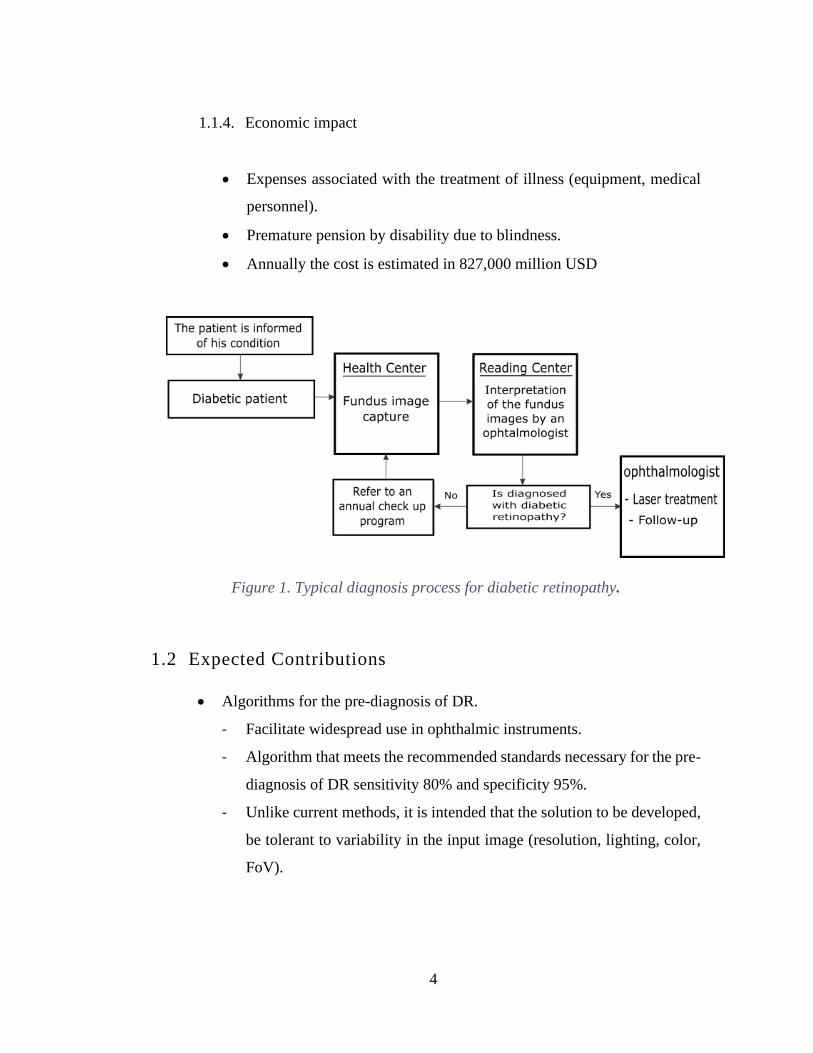
enough ophthalmologist to cover the demand of eye exams. In the Figure 1 is shown
the typical diagnosis process of the diabetic retinopathy, which carries a great load
of time for ophthalmologists inspecting the fundus images. It is necessary to de-
velop systems that can monitor and locate in a reliable and efficient way the abnor-
malities present in the images of the fundus. Some relevant facts about the diabetic
retinopathy, classified in four areas are:
1.1.1. Statistics
• By 2030, the number of people with diabetes will increase by 3.4 times
of those in 2014, while growth in the number of ophthalmologists will
be only 2%[1].

3
• Moreover, the number of diabetics worldwide is underestimated. In [2]
a study established that deaths attributable to complications of diabetes
in the US are not taken into account.
• On a IAPB report [3] is assured that approximately 50% of people with
diabetes are currently undiagnosed.
• In Mexico City, complications caused by diabetes are the leading cause
of death [4].
• Diabetic retinopathy affects approximately 80% of people who have
suffered from diabetes for 10 years or more [5].
• Worldwide, DR is cause number one for blindness of people on working
age [6].
1.1.2. Health area impact
• In Mexico, there are currently 3,500 registered ophthalmologists and a
population of diabetics of 14 million [7], if the burden of people is di-
vided equally by ophthalmologist, each should examine 4,000 patients
and the time it would take to complete the analyzes would be 333 days
per specialist.
• A low percentage of diabetics get tested. In the US, only 4 out of 10
diabetics perform their eye fundus examination per year [8].
1.1.3. Social impact
• Cost per exam.
• The duration of the examination for the patient is 2 to 3 hours with di-
lation of the pupil.
• Waiting time for consultation with the ophthalmologist. In the public
sector, it is typically 4 to 12 weeks and 1 to 3 weeks in the private sector.
4
1.1.4. Economic impact
• Expenses associated with the treatment of illness (equipment, medical
personnel).
• Premature pension by disability due to blindness.
• Annually the cost is estimated in 827,000 million USD
Figure 1. Typical diagnosis process for diabetic retinopathy.
1.2 Expected Contributions
• Algorithms for the pre-diagnosis of DR.
- Facilitate widespread use in ophthalmic instruments.
- Algorithm that meets the recommended standards necessary for the pre-
diagnosis of DR sensitivity 80% and specificity 95%.
- Unlike current methods, it is intended that the solution to be developed,
be tolerant to variability in the input image (resolution, lighting, color,
FoV).
5
- As for the classification, unlike most methods found in the literature that
employ on the order of 100’s of characteristics, it will be sought to re-
duce this number, seeking those that reflect the knowledge of the expert.
• Contribute to the early pre-diagnosis
- Make it easier to take the exam at least twice a year.
- No pupil dilation.
- No need for ophthalmologist for pre-diagnosis.
1.3 Objectives
1.3.1 General objective
Design and develop a solution for the detection of two anatomical struc-
tures, one lesion associated with diabetic retinopathy and a pre-diagnosis
of one retinal disease in color images of eye fundus, using multiple public
image databases with different resolutions, that compete with current state
of the art publications.
1.3.2 Specific objectives
1. Design and develop method(s) for the detection of one lesion asso-
ciated with diabetic retinopathy, two anatomical structures of the ret-
ina and a pre-diagnosis of one retinal disease.
2. To develop a method for detecting lesions associated with diabetic
retinopathy that presents a competitive performance in terms of sen-
sitivity and specificity, according to The British Diabetic

6
Retinopathy Working Group these values should be at least 80% and
95% respectively [9].
3. Evaluate the results in 4 different databases of public access that in-
clude variety of pathologies, resolution and image quality to verify
that the algorithm can be parameterized for different databases.
7
State of the art
2.1 Fundus Image Pre-processing
The fundus images are acquired by the reflection of visible light of the fundus of
the retina and are captured using a fundus camera, obtaining a 2-D representation
of the retinal tissues projected on the plane of the image. The medical images are
typically acquired following a defined protocol, in order to ensure that the appear-
ance of the structures is similar in any image that is acquired using the same proto-
col; however, the fundus images obtained from the monitoring programs are ac-
quired in different environments using different fundus camera models which are
operated by qualified technical personnel with different levels of experience, lead-
ing to a variation in the quality of the images. The above, added to a poor dynamic
range of the fundus camera sensor and other characteristics of the equipment and
its use, can generate images of low diagnostic quality. In this context, the notion of
quality in the fundus images refers to the ability of an expert (computer-assisted
ophthalmologist or diagnosis by a specialized physician) to correctly assess the pa-
tient's condition through the fundus image. In approximately 10% of the images of
the retina, the artifacts present are significant enough to prevent their evaluation by
an expert [10], and it is presumed that a similar ratio is inadequate for automatic
analysis.
Fundus images present a large variability which can be classified in two main
groups: intra-image variations and inter-image variations. Intra-image variations
arise due to differences in light diffusion, the presence of abnormalities, variation
in fundus reflectivity and fundus thickness. Differences between images (inter-im-
age variability) may be caused by factors including differences in camera sensors,
illumination, acquisition angle and retinal pigmentation which highly variates
among patient ethnicity. The following describes some of these unwanted charac-
teristics and that occur in the data sets.
8
• Non-uniform illumination: Despite having controlled conditions at the time of
image taking, a large number of fundus images present a non-uniform illumi-
nation, which is originated due to different factors, such as: the curved surface
of the retina, the pupil size (of great variability between patients), the alignment
of the eye with the optical axis of the camera, and the direction and shape of the
lighting source, cleanness of the lens, among others.
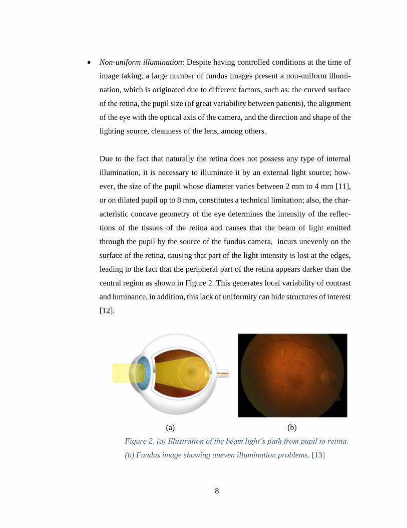
Due to the fact that naturally the retina does not possess any type of internal
illumination, it is necessary to illuminate it by an external light source; how-
ever, the size of the pupil whose diameter varies between 2 mm to 4 mm [11],
or on dilated pupil up to 8 mm, constitutes a technical limitation; also, the char-
acteristic concave geometry of the eye determines the intensity of the reflec-
tions of the tissues of the retina and causes that the beam of light emitted
through the pupil by the source of the fundus camera, incurs unevenly on the
surface of the retina, causing that part of the light intensity is lost at the edges,
leading to the fact that the peripheral part of the retina appears darker than the
central region as shown in Figure 2. This generates local variability of contrast
and luminance, in addition, this lack of uniformity can hide structures of interest
[12].
(a) (b)
Figure 2. (a) Illustration of the beam light’s path from pupil to retina.
(b) Fundus image showing uneven illumination problems. [13]

9
• Low contrast: In image processing, contrast is defined as the variation in color
perceived in an image. Contrast enhancement techniques aim to facilitate the
visual interpretation of an image by altering the visual appearance that makes
an object (or its representation in an image) distinguishable from other objects
and background.
In practice, an inadequate focusing, bad positioning, poor illumination or eye
movement make that the fundus images acquired present a low contrast. Addi-
tionally, the narrow thickness of the blood vessels causes the contrast between
the veins and the retina tissue to be low in the obtained fundus images [14]. On
the other hand, the contrast is affected by the non-uniform distribution of light-
ing as it causes shadows and internal reflections in the image.
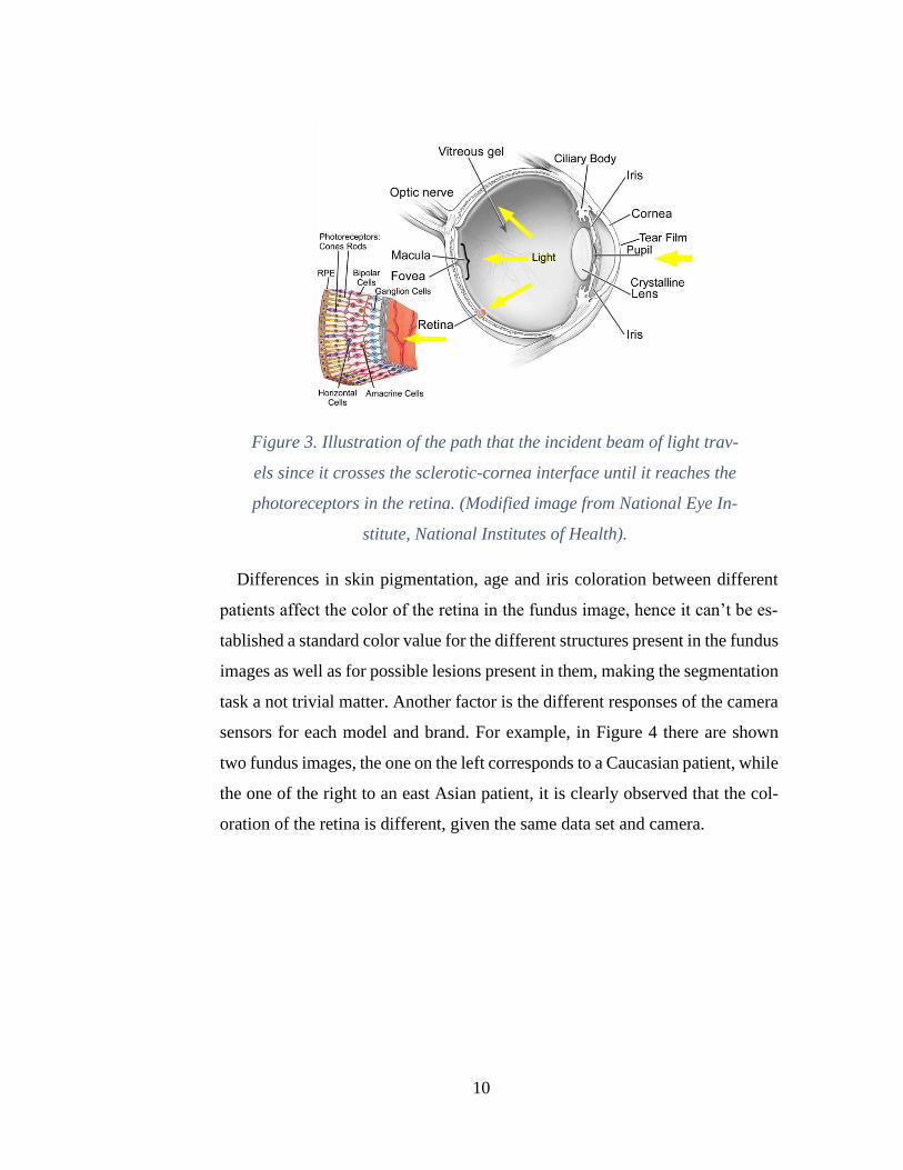
• Color variability: The human eye is a complex optical structure sensitive to
wavelengths in the range of 380 nm to 760 nm. The beam of light entering the
eye is refracted when it passes from the air through the sclerotic-cornea inter-
face. Then, it continues its journey through aqueous humor and the pupil (dia-
phragm controlled by the iris) where it is refracted again by the lens before
passing through the vitreous humor and finally reaches the retina, where it is
absorbed by the cones and rods after crossing several layers of tissue Figure 3.
The sclerotic-cornea and crystalline interface are the most refractive compo-
nents in the eye and together act as a compound lens to project an inverted
image on the retina, the light sensitive tissue of the eye. From the retina, the
electrical signals are transmitted to the visual center of the brain through the
optic nerve [15].
10
Figure 3. Illustration of the path that the incident beam of light trav-
els since it crosses the sclerotic-cornea interface until it reaches the
photoreceptors in the retina. (Modified image from National Eye In-
stitute, National Institutes of Health).
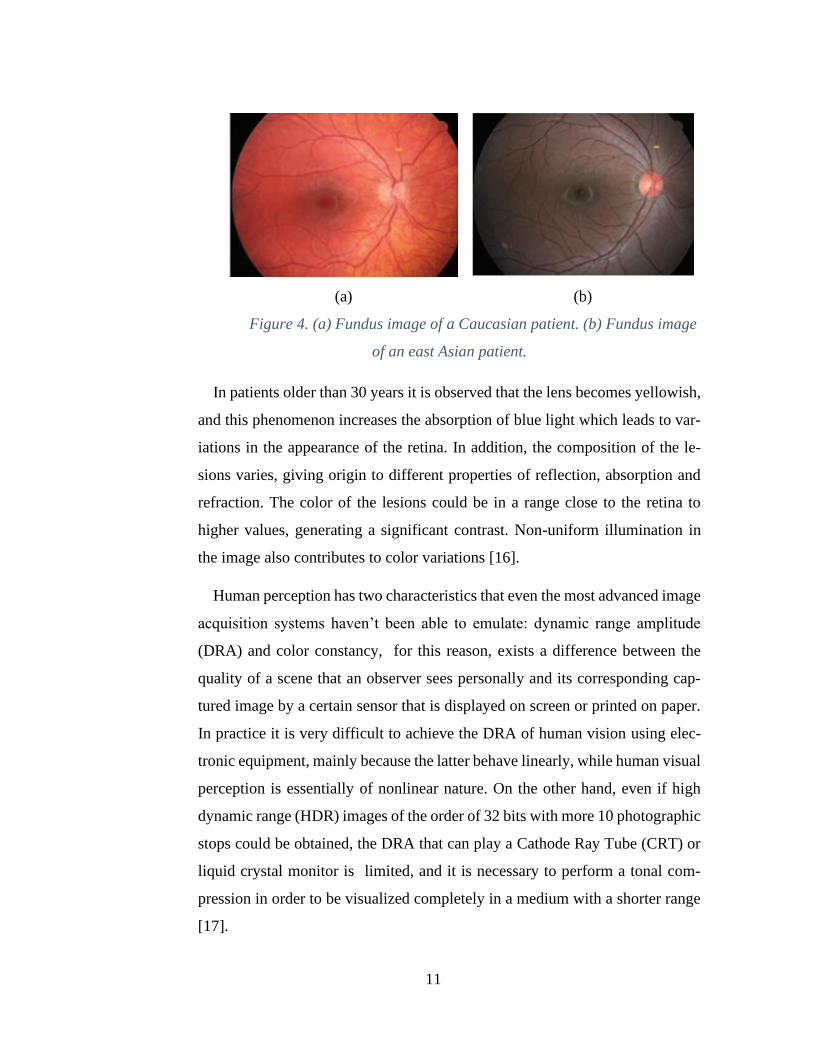
Differences in skin pigmentation, age and iris coloration between different
patients affect the color of the retina in the fundus image, hence it can’t be es-
tablished a standard color value for the different structures present in the fundus
images as well as for possible lesions present in them, making the segmentation
task a not trivial matter. Another factor is the different responses of the camera
sensors for each model and brand. For example, in Figure 4 there are shown
two fundus images, the one on the left corresponds to a Caucasian patient, while
the one of the right to an east Asian patient, it is clearly observed that the col-
oration of the retina is different, given the same data set and camera.
11
(a) (b)
Figure 4. (a) Fundus image of a Caucasian patient. (b) Fundus image
of an east Asian patient.
In patients older than 30 years it is observed that the lens becomes yellowish,
and this phenomenon increases the absorption of blue light which leads to var-
iations in the appearance of the retina. In addition, the composition of the le-
sions varies, giving origin to different properties of reflection, absorption and
refraction. The color of the lesions could be in a range close to the retina to
higher values, generating a significant contrast. Non-uniform illumination in
the image also contributes to color variations [16].
Human perception has two characteristics that even the most advanced image
acquisition systems haven’t been able to emulate: dynamic range amplitude
(DRA) and color constancy, for this reason, exists a difference between the
quality of a scene that an observer sees personally and its corresponding cap-
tured image by a certain sensor that is displayed on screen or printed on paper.
In practice it is very difficult to achieve the DRA of human vision using elec-
tronic equipment, mainly because the latter behave linearly, while human visual
perception is essentially of nonlinear nature. On the other hand, even if high
dynamic range (HDR) images of the order of 32 bits with more 10 photographic
stops could be obtained, the DRA that can play a Cathode Ray Tube (CRT) or
liquid crystal monitor is limited, and it is necessary to perform a tonal com-
pression in order to be visualized completely in a medium with a shorter range
[17].
12
In eye fundus images, the intensity of each pixel represents the amount of
light reflected by the wavelengths of the Red, Green and Blue channels (RGB);
however, if pictures of the same retina are taken with two different fundus cam-
eras, the content in the Red, Green and Blue channels of the RGB color space
of the lesions would be different because to changes in the illumination and the
characteristic sensitivity of the camera sensor. The Photometric information
should be consistent in all images that present the same injury or structure of
interest; however, there are several natural sources that cause variations in pho-
tometric information, such as: changes in the device of acquisition of the image
or its parameters and/or changes in the lighting source (spectral changes that
depend on the type of lighting source and the surrounding illumination condi-
tions; such as time of use , a room with windows with or without shades.
The best solution to standardize the fundus images would be to calibrate the
image acquisition system; however, the fundus images are typically captured
by uncalibrated systems with unknown parameters, reason whereby there is no
photometric consistency between the images.
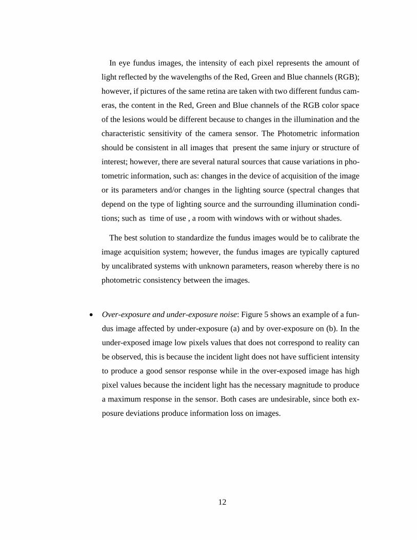
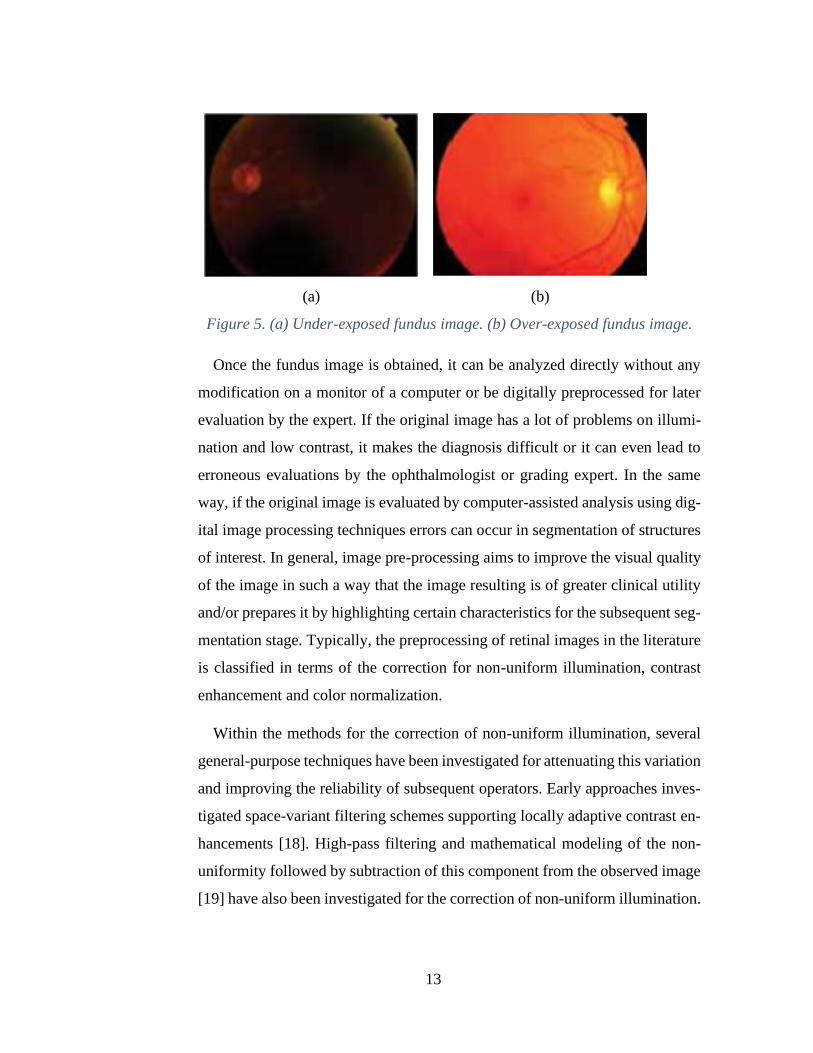
• Over-exposure and under-exposure noise: Figure 5 shows an example of a fun-
dus image affected by under-exposure (a) and by over-exposure on (b). In the
under-exposed image low pixels values that does not correspond to reality can
be observed, this is because the incident light does not have sufficient intensity
to produce a good sensor response while in the over-exposed image has high
pixel values because the incident light has the necessary magnitude to produce
a maximum response in the sensor. Both cases are undesirable, since both ex-
posure deviations produce information loss on images.
13
(a) (b)
Figure 5. (a) Under-exposed fundus image. (b) Over-exposed fundus image.
Once the fundus image is obtained, it can be analyzed directly without any
modification on a monitor of a computer or be digitally preprocessed for later
evaluation by the expert. If the original image has a lot of problems on illumi-
nation and low contrast, it makes the diagnosis difficult or it can even lead to
erroneous evaluations by the ophthalmologist or grading expert. In the same
way, if the original image is evaluated by computer-assisted analysis using dig-
ital image processing techniques errors can occur in segmentation of structures
of interest. In general, image pre-processing aims to improve the visual quality
of the image in such a way that the image resulting is of greater clinical utility
and/or prepares it by highlighting certain characteristics for the subsequent seg-
mentation stage. Typically, the preprocessing of retinal images in the literature
is classified in terms of the correction for non-uniform illumination, contrast
enhancement and color normalization.
Within the methods for the correction of non-uniform illumination, several
general-purpose techniques have been investigated for attenuating this variation
and improving the reliability of subsequent operators. Early approaches inves-
tigated space-variant filtering schemes supporting locally adaptive contrast en-
hancements [18]. High-pass filtering and mathematical modeling of the non-
uniformity followed by subtraction of this component from the observed image
[19] have also been investigated for the correction of non-uniform illumination.
14
Among the techniques for color normalization, are those that make use of the
histogram specification [20] to ensure that all sample images match a distribu-
tion of a reference image; however, making a fundus image coincident with a
reference model may lead to potentially masking specific lesion characteristics
found in the original histogram. The reference model is usually obtained from
an image that shows good contrast and color in accordance to the judgment of
an expert. Another technique used is the color transfer [21] in which color char-
acteristics are transferred from one image to another based on simple statistics
of the image, the first step is to transform the images to a color space that min-
imizes the correlations between the color channels, then the means and standard
deviations of the images are matched.
In the literature, there is a great variety of methods for improving contrast,
aiming to increase the level of differentiation of the characteristics of the retina.
These techniques are usually applied after correcting non-uniform illumination
and normalizing the color of the images. Conventional methods based on the
global histogram of the image such as contrast stretching and histogram equal-
ization tend to result in loss of information in the brightest areas as well as in
the dark areas of the background image, which is why adaptive enhancement of
the histogram with limited contrast (CLAHE) [22] is most commonly used.
2.2 Retinal structures location
The location of the different normal ocular fundus structures such as: blood
vessels, optic disc, macula and fovea, it is common within most of systems ded-
icated to the automatic detection of the early signs of diabetic retinopathy. In
particular, the location of the optic disc, which corresponds to the visible part
of the optic nerve in the eye, is an important task in systems dedicated to the
detection of exudates since the optic disc shares similar characteristics of color
and brightness, which can cause sections of it to be potentially erroneously

15
detected as exudates, negatively affecting system performance. This can be
avoided if optic’s disc location is known in advance. Additionally, the state of
the optical disc is important in diseases such as glaucoma, diabetic optic neu-
ropathy and other pathologies related to the optic nerve. The fovea is located in
the center of the macula and is the area of the retina that is used for fine vision.
Retinopathy in this area is associated with a high risk of vision loss, for this
reason it is very important to locate these two areas in order to prevent compli-
cations.
• Optic Disc (OD) Location
The OD is the exit point of retinal nerve fibers from the eye, and the entrance
and exit point for retinal blood vessels. It is a brighter region than the rest of the
ocular fundus and its shape is round when healthy. Although the OD main fea-
tures and characteristics are relatively easy to describe, individual differences,
diseases and other factors will influence characteristics of the optic disc, making
its automatic localization a difficult task. Image quality can also affect the ap-
pearance of the OD. A retinal image may be unevenly illuminated or poorly
focused, resulting in a less distinct and/or blurred OD. Optic disc location meth-
odology involves extensive research interest [23], due to its relevance for OD
diseases and as an anatomic eye’s feature. The location of OD is important in
retinal image analysis because it is a key reference for recognition algorithms
[24], blood vessels segmentation [25], and diagnosing some diseases such as
diabetes and for registering changes within the optic disc region due to diseases
such as glaucoma and the development of new blood vessels [26]. The OD is
also a landmark for other retinal features, such as the distance between the OD
and the fovea [27], which is often used for estimating the location of the macula
[28] and is also used as a reference length for measuring distances in retinal
images. In addition, it is important to detect and isolate OD region because,
16
most of the algorithms designed to segment/detect abnormalities such as hard
exudates in DR will detect lots of false positives in OD region as the color tone
of the OD is like the hard exudates. Accurate identification of OD can be used
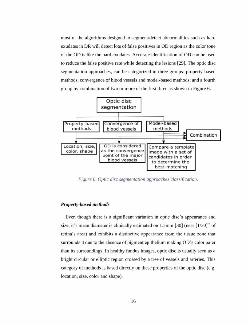
to reduce the false positive rate while detecting the lesions [29]. The optic disc
segmentation approaches, can be categorized in three groups: property-based
methods, convergence of blood vessels and model-based methods; and a fourth
group by combination of two or more of the first three as shown in Figure 6.
Figure 6. Optic disc segmentation approaches classification.
Property-based methods
Even though there is a significant variation in optic disc’s appearance and
size, it’s mean diameter is clinically estimated on 1.5mm [30] (near [1/30]th of
retina’s area) and exhibits a distinctive appearance from the tissue zone that
surrounds it due to the absence of pigment epithelium making OD’s color paler
than its surroundings. In healthy fundus images, optic disc is usually seen as a
bright circular or elliptic region crossed by a tree of vessels and arteries. This
category of methods is based directly on these properties of the optic disc (e.g.
location, size, color and shape).

17
Pourreza-Shahri et al. [31] detection method is based on the fact that OD
appears as a bright region in a fundus image. Radon transform (RT) is used to
generate the integration of pixel intensities along different directions which
leads to making Optic Nerve Head (ONH) a prominent structure in the Radon
space. Only brightness information is considered in order to gain high pro-
cessing speeds. This method claims to be computationally efficient without ev-
idence, a fundus image is first partitioned into overlapping blocks or sub-im-
ages. RT is applied to each block or sub-image and the sub-images exhibiting
peaks in the Radon space are then processed to locate the OD. It was reported
a detection rate of 100% and 96.3% on DRIVE and STARE dataset respec-
tively. The average computation time for the algorithm for STARE database
was 2.9 s, using an Intel Core2Duo 3.33 GHz PC.
Rahebi & Hardalac [32] implemented a firefly algorithm to detect the optic
disc in retinal fundus images. The firefly intelligent algorithm is an emerging
intelligent algorithm that was inspired by the social behavior of fireflies. This
algorithm was initially introduced at Cambridge University by Yang in 2008
[33]. The population in this algorithm includes the fireflies, each of which has
a specific rate of lighting or fitness. In this method, the insects are compared
two by two, and the less attractive insects can be observed to move toward the
more attractive insects. Finally, one of the insects is selected as the most attrac-
tive, and this insect presents the optimum response to the problem in question.
The light intensity of the pixels of the retinal image pixels is used instead of
firefly lightings. The movement of these insects due to local fluctuations pro-
duces different light intensity values in the images. Because the optic disc is the
brightest area in the retinal images, all the insects move toward brightest area
and thus specify the location of the optic disc in the image. The results of their
algorithm showed a success rate of optic disc localization of 94.38%, 100% and
95% on DIARETDB1, DRIVE and STARE dataset respectively. The average
18
computation time was 2.13 s for DRIVE, 2.81 s for STARE and 3.52 s for DI-
ARETDB1 using a PC with an Intel Duo CPU, 2.00 GHz RAM.
Algorithms which relied solely on OD’s properties showed to be simple, fast
and reasonably robust for OD localization in normal retinal images with low
variation between images. On the other hand, these algorithms may fail when
there are distracters such as exudates and bright artifacts [34] in the fundus im-
ages, as well as when OD is obscured by blood vessels or in the case where OD
is only partially visible.
Convergence of blood vessels
This type of method approaches location of optic disc by using the infor-
mation provided by the vascular structure of the retina, since the optic nerve is
the focal point of the retina’s blood vessel network [35]. To locate optic disc by
this method, the retinal blood vessel network is first detected.
Soares et al. [36] proposed an algorithm with a new vessel enhancement
method based on a modified corner detector. A weighted version of the vessel
enhancement is combined with morphological operators, to detect the four main
vessels orientations {0o, 45o, 90o, 135o}. These four image functions determine
an initial optic disc localization, resulting in two images vertical or horizontal
orientations. Each division is averaged creating a 2D step function, and a cu-
mulative sum of the different sizes step functions is calculated in the 2 orienta-
tions, resulting in an initial optic disc position. The final OD is determined by
a vessel convergence algorithm using its two most relevant features; high vas-
culature convergence and high intensity values. This approach claims to be ro-
bust since it was evaluated in eight publicly-available datasets. Another relevant
aspect the proposed method is that it allows a considerable illumination vari-
ance, since no illumination equalization was performed as in other methods.
The authors reported a detection accuracy of 98.88%, 100%, 99.25%, 98.77%,

19
98.78%, 98.46%, 99% and 100% on DIARETDB1, DRIVE, MESSIDOR,
STARE, E-OPHTA, DIARETDB0, ROC and HRF datasets respectively. The
optic disc was localized correctly in 1752 out of the 1767 retinal images
(99.15%) with an average computation time of 18.34 seconds. The method was
implemented on a laptop with 2 GHz Intel Core i7 and 6 GB of RAM.
Marin et al. [37] approach consists on performing a set of iterative opening–
closing morphological operations on the original fundus image intensity chan-
nel to produce a bright region-enhanced image. Taking blood vessel confluence
at the OD into account, a 2-step automatic thresholding procedure is then ap-
plied to obtain a reduced region of interest, where the center and the OD pixel
region are finally obtained by performing the circular Hough transform on a set
of OD boundary candidates generated through the application of the Prewitt
edge detector. The proposed method claims to be a suitable tool for integration
into an automated prescreening system, due to its proven effectiveness and ro-
bustness, together with its simplicity. Jaccard and dice’s coefficients are 0.87
and 0.92 for MESSIDOR dataset and 0.85 and 0.92 MESSIDOR-2 dataset. The
average computational time was 5.425 s running on a PC with a dual- Intel Xeon
CPU at 32Ghz and 32 GB of RAM capacity.
Wu et al. [38] presented a novel method to automatically localize ODs in
retinal fundus images based on directional models. According to the character-
istics of retina vessel networks, such as their origin at the OD and parabolic
shape of the main vessels, a global directional model, named the relaxed bi-
parabola directional model (R-BPDM), is first built. The main vessels are mod-
eled by using two parabolas with a shared vertex and different parameters. A
local directional model, named the disc directional model (DDM), is built to
characterize the local vessel convergence in the OD as well as the shape and the
brightness of the OD. Finally, the global and the local directional models are
integrated to form a hybrid directional model, which can exploit the advantages
of the global and local models for highly accurate OD localization. The method
20
proved to be effective by being evaluated on nine publicly available databases
(DRIVE, STARE, ARIA, MESSIDOR, DIARETDB1, DIARETDB0, ROC,
ONH and DRIONS), achieving an accuracy of 100% for each database.
Optic disc segmentation methods based on convergence of blood vessels
seem to be the most efficient way to localize the optic disc in terms of accuracy
and robustness; at the expense of greater time execution.
Model-based methods
The model-based methods rely in the fact that optic disc shape is approxi-
mately circular and that the pixels conforming its area are brighter than its sur-
roundings. The method consists on comparing a template image (model) with a
group of candidates in the fundus image, with the purpose of determine the can-
didate that exhibits the best match. The created template is applied as a running
window of NxN size along the fundus image and the correlation between the
template and the section of the image is calculated, the region with the highest
correlation is selected as the OD region.
Dashtbozorg et al. [39] developed an automatic approach for OD segmenta-
tion using a multiresolution sliding band filter (SBF). A high-resolution SBF is
applied to obtain a set of pixels associated with the maximum response of the
SBF, giving a coarse estimation of the OD boundary, which is regularized using
a smoothing algorithm. The algorithm segments the optic disc independently of
image characteristics such as size and camera field of view and claims to be
robust to variations of contrast and illumination, the presence of exudates and
peripapillary atrophy caused by diabetic retinopathy, risk of macular edema,
and the blurredness of images due to severe cataracts. The results on terms of
overlapping score (S) are 0.88, 0.83 and 0.85 for MESSIDOR, ONH and IN-
SPIRE-AVR datasets respectively. The algorithm was implemented using an
21
Intel CPU i7-2600k, 3.40 GHz, 8 GB RAM computer. The average running
time was 10.6 s per image in the MESSIDOR dataset.
Wang et al. [40] used a template matching method to approximately locate
the optic disc center, and the blood vessel is extracted to reset the center. This
is followed by applying the Level Set Method, which incorporates edge term,
distance-regularization term and shape-prior term, to segment the shape of the
optic disc. Has advantages over the shape-based template matching method as
it addresses the obstruction of the vessels inside the optic disc area and the in-
tensity inhomogeneity. Authors reported a sensitivity of 93.24%, 92.58% and
94.65% on DIARETDB1, DRIVE and DIARETDB0 datasets respectively. The
average computation time reported is 17.55 seconds for DRIVE, 18.25 seconds
for DIARETDB1, and 18.3 seconds for DIARETDB0 on an Intel(R) Core(TM)
i5-2500 CPU, clock of 3.3GHz, and 8G RAM memory PC.
Mary et al. [41] used an active contour model (ACM). An OD segmentation
scheme is designed to infer how the performance of the well-known gradient
vector flow (GVF) model compares with nine popular/recent ACM algorithms
by supplying them with the initial OD contour derived from the circular Hough
transform. This article gives a systematic performance comparison of a judi-
cious choice of ten widely recommended ACM techniques, which are employed
to segment the OD from 169 annotated retinal fundus images of various cate-
gories. The outcome of the study suggests that the GVF-based Xu-ACM initial-
ized with the contour produced by the CHT outclasses the rest of the state-of-
the-art variants of ACM. The result in terms of Hausdorff distance value is
33.49 ± 18.21 for RIM-ONE dataset.
Molina-Casado et al. [42] approach consists in a pre-processing stage inclu-
ding intensity normalization using a contrast stretching method and resizing of
the original retinal image. Next, the detection of the set of OD candidates is
done using correlation with template matching (TM). The template consists of
a set of three squared shape objects with width of four times the OD radius size.

22
Finally, using inter-structure relational knowledge (i.e., distance relations with
another retinal structures as macula and veins), false candidates are eliminated.
The success rates reported were: 99.33% for MESSIDOR, 96.63% for Di-
aretdb1, 100% for DRIONS and 100% for ONHSD.
The approaches based on vessels-convergence and template matching proved
to achieve better sensitivity rates than that achieved by the property-based meth-
ods, since the number of false responses were greatly reduced in the presence
of other similar abnormal artifacts. But, on the other hand, such approaches ob-
viously take more processing time than property-based methods [23].
Combination of methods
This group correspond to those OD segmentation methods that don’t rely
only on the OD’s properties, convergence of vessels or matching a template.
Instead they combine two or more of the above methods exposed.
Harangi & Hajdu [43] stated that there´s no reason to assume that any single
algorithm would be optimal for the detection of various anatomical parts of the
retina. It is difficult to determine which the best approach is, because good re-
sults were reported for healthy retinas but weaker ones for more challenging
datasets containing diseased retinas with variable appearance of ODs in term of
intensity, color, contour definition and so on. To overcome this, they studied
and adapted some of the state-of-the-art OD detectors and finally organized
them into an ensemble framework in order to combine their strengths and max-
imize the accuracy of the localization of the OD. Authors reported a sensitivity
of 98.88%, 100%, 98.33% and 98.46% on DIARETDB1, DRIVE, MESSIDOR
and DIARETDB0 datasets respectively.
Ren et al. [44] based the identification of OD location candidate regions on
high-intensity feature and vessels convergence property. Secondly, a line oper-
ator filter for circular brightness feature detection is designed to locate the OD

23
accurately on candidates. Thirdly, an initialized contour is obtained by iterative
thresholding and ellipse fitting based on the detected OD position. Finally, a
region-based active contour model in a variationally level set formulation and
ellipse fitting are employed to estimate the OD boundary. The reported sensi-
tivity on MESSIDOR database was 98.67%.
Qureshi et al. [28] proposed an efficient combination of algorithms for the
automated localization of the optic disc and macula in retinal fundus images.
An ensemble of algorithms based on different principles can be more accurate
than any of its individual members if the individual algorithms are doing better
than random guessing. They suggested an approach to automatically combine
different optic disc and macula detectors, to benefit from their strengths while
overcoming their weaknesses. Authors reported a detection percentage of
97.79, 100 and 97.64 on DIARETDB1, DRIVE and DIARETDB0 respectively.
Basit & Fraz [45] method for automatic detection of the optic disc locus and
optic disc boundary extraction is proposed based on morphological operations,
regional properties, and marker-controlled watershed transform. The claimed
advantages over other methods are: it works well on a vast variety of illumina-
tions present in retinal images, it only extracts the main blood vessels centerline
from the image and the combination of extracted vessels centerline and local
maxima make the proposed method more tolerant to error for the optic disc
location. The reported sensitivity on DIARTEDB1, DRIVE and CHASE_DB1
databases was 73.47%, 89.21% and 48.34% respectively.
Xiong & Li [46] approach has three main steps: region-of-interest detection,
candidate pixel detection, and confidence score calculation. The features of ves-
sel direction, intensity, OD edges, and size of bright regions were extracted and
employed in the proposed OD locating approach. Authors claim that compared
with the methods using vessel edge information only, the improvement on can-
didate pixel detection and the confidence value achieves promising results in
the following situations: the images with dark OD due to uneven illumination
24
and low contrast; the retinal images with incomplete OD; the images with bright
exudates, whose size and intensity are similar to OD. The results on terms of
success rate of OD localization are 97.8%, 100%, 95.8% and 99.2% on DI-
ARETDB1, DRIVE, STARE and DIARETDB0 databases respectively.
Haloi et al. [47] used a saliency map based method to detect the optic disc
followed by an unsupervised probabilistic Latent Semantic Analysis for detec-
tion validation. The validation concept is based on distinct vessels structures in
the optic disc. By using the clinical information of standard location of the fovea
with respect to the optic disc, the macula region is estimated. Authors claim that
this method gives 100% accuracy in optic disc detection in different challenging
images with pathological symptoms. Reported detection accuracies are 100%,
100%, 98.8% on DIARETDB1, MESSIDOR and STARE datasets respectively.
Díaz-Pernil et al. [48] proposed a method where image edges are extracted
using a new operator, called A Graphical P segmentation (AGP-color segmen-
tation), which is a variation of the Sobel operator. The resulting image is bina-
rized with Hamadani's technique and, finally, a new algorithm called Hough
circle cloud is applied for the detection of the OD. The proposed algorithm con-
siders the complete RGB color space for image processing and does not need
any parameter to be fixed. Reported sensitivities for DIARETDB1 and DRIVE
datasets are 91.8% and 89.9% respectively. The mean consumed time per image
is 7.6 and 16.3 s for DRIVE and DIARETDB1, respectively. The algorithm was
implemented on a computer with a CPU AMD Athlon II ×4 645 and 4 GB
DDR3 to 1600 MHz of main memory.
Fan et al. [49] method employed supervised learning to train an OD edge
detector by using structured learning. The edge detector is applied to the three
channels of RGB and an optimal set of edge features is calculated automatically
using the random forest classifier for each channel. Next, thresholding is per-
formed on the edge map, obtaining a binary image of the OD. Finally, circle
Hough transform is applied to approximate the boundary of OD by a circle. The
25
authors reported an overlap area of 0.86, dice coefficient of 0.91, accuracy of
0.97, and a true positive and false positive fraction of 0.91 and 0.01 for the
MESSIDOR, DRIONS and ONHSD public datasets overall. The average com-
putational time obtained for OD segmentation is 1.7494 s. The algorithm was
implemented using a PC with an Intel (R) Core (TM) i-5 4210 M CPU at 2.60
GHZ and 4 GB of RAM.
Discussion
The optic disc segmentation algorithms were classified into four groups:
property-based methods, convergence of blood vessels methods, model-based
methods and combination of methods. However, direct comparison is difficult
because different groups of researchers tend to use different metrics, image da-
tabases and number of images to train the classifier to measure the performance
of their algorithms. Consequently, it is difficult to do a meaningful comparison
among them. Despite using the same evaluation measures, different implemen-
tations of the metrics may influence the final results [50]. As a remark, it is
important to differentiate between OD segmentation, OD localization and OD
detection. OD detection output will be the position, or a bounding box of the
OD if it exists in the image, while OD’s localization goal is to delimitate the
OD’s region more accurately and OD segmentation is the process of assigning
a label to every pixel in fundus image that belongs to the OD.
From the reviewed literature, the methods based on the properties of the optic
disc (shape, brightness, size, etc.) achieved good results in fundus images where
absent or slightly abnormalities were present, but these methods usually failed
to detect the optic disc in pathological images where abnormalities, such as
large clusters of exudates were present, confusing them with the optic disc due
to their similar properties. Therefore, diverse OD segmentation approaches that
not only rely on the properties of the optic disc were followed by researchers.
26
Among these approaches, a recurrent one is: convergence of blood vessels
methods, which exploits information provided by the vascular tree of the retina,
since the optic disc is considered as the convergence point of the major blood
vessels. This group of methods achieve better sensitivity rates than those
achieved by the property-based methods, since the number of false responses
were greatly reduced in the presence of large clusters of exudates and bright
artifacts. But, as a drawback, these approaches take more processing time than
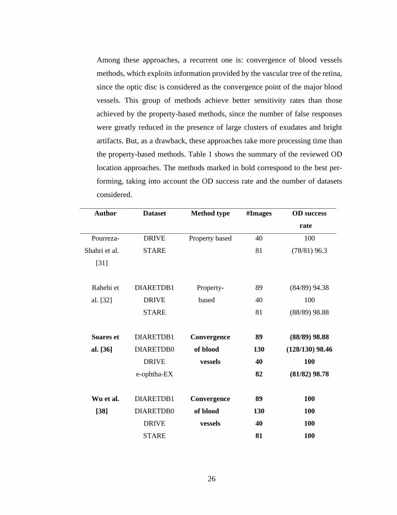
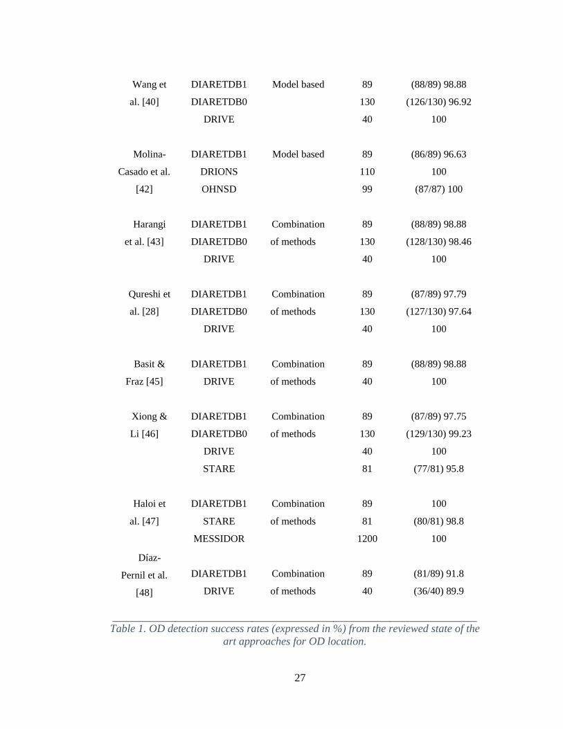
the property-based methods. Table 1 shows the summary of the reviewed OD
location approaches. The methods marked in bold correspond to the best per-
forming, taking into account the OD success rate and the number of datasets
considered.
Author Dataset Method type #Images OD success
rate
Pourreza-
Shahri et al.
[31]
DRIVE
STARE
Property based 40
81
100
(78/81) 96.3
Rahebi et
al. [32]
Soares et
al. [36]
Wu et al.
[38]
DIARETDB1
DRIVE
STARE
DIARETDB1
DIARETDB0
DRIVE
e-ophtha-EX
DIARETDB1
DIARETDB0
DRIVE
STARE
Property-
based
Convergence
of blood
vessels
Convergence
of blood
vessels
89
40
81
89
130
40
82
89
130
40
81
(84/89) 94.38
100
(88/89) 98.88
(88/89) 98.88
(128/130) 98.46
100
(81/82) 98.78
100
100
100
100
27
Wang et
al. [40]
Molina-
Casado et al.
[42]
Harangi
et al. [43]
Qureshi et
al. [28]
Basit &
Fraz [45]
Xiong &
Li [46]
Haloi et
al. [47]
Díaz-
Pernil et al.
[48]
DIARETDB1
DIARETDB0
DRIVE
DIARETDB1
DRIONS
OHNSD
DIARETDB1
DIARETDB0
DRIVE
DIARETDB1
DIARETDB0
DRIVE
DIARETDB1
DRIVE
DIARETDB1
DIARETDB0
DRIVE
STARE
DIARETDB1
STARE
MESSIDOR
DIARETDB1
DRIVE
Model based
Model based
Combination
of methods
Combination
of methods
Combination
of methods
Combination
of methods
Combination
of methods
Combination
of methods
89
130
40
89
110
99
89
130
40
89
130
40
89
40
89
130
40
81
89
81
1200
89
40
(88/89) 98.88
(126/130) 96.92
100
(86/89) 96.63
100
(87/87) 100
(88/89) 98.88
(128/130) 98.46
100
(87/89) 97.79
(127/130) 97.64
100
(88/89) 98.88
100
(87/89) 97.75
(129/130) 99.23
100
(77/81) 95.8
100
(80/81) 98.8
100
(81/89) 91.8
(36/40) 89.9
Table 1. OD detection success rates (expressed in %) from the reviewed state of the
art approaches for OD location.
28
2.3 Diabetic Macular Edema (DME)
Diabetic Macular Edema is an important complication of diabetic retinopathy
and one of the worldwide leading causes of partial or total vision loss [51].
Diabetes Mellitus is the primary cause of DME and DR and is characterized by
the appearance of pathologies and retinal vessel damage. In diabetes mellitus,
the blood glucose level raises due to disturbance in insulin dynamics. The high
blood glucose concentration affects the blood vessels along with the nerve cells
inside the kidneys, brain, heart, and eyes. Worldwide, 93 and 21 million people
are affected by DR and DME respectively, and their prevalence are of 6.96%
and 10.2%, respectively [52].
All patients who have been diagnosed with diabetes, either type 1 or type 2,
are at risk of developing DR and DME. DR is a progressive disease of the retina
that involves pathological changes of the blood vessels, and consequently re-
sults in the presence of one or more abnormal features recognizable by a trained
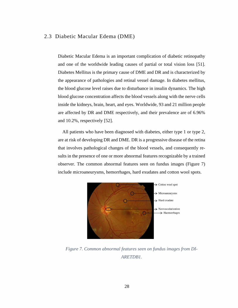
observer. The common abnormal features seen on fundus images (Figure 7)
include microaneurysms, hemorrhages, hard exudates and cotton wool spots.
Figure 7. Common abnormal features seen on fundus images from DI-
ARETDB1.

29
The progression of DR can be divided into several stages. First, as the blood
glucose level increases, the permeability of the capillaries increases and there
is a loss of elasticity of the endothelial capillary wall. This is the stage of mild
non-proliferative diabetic retinopathy (NPDR). The appearance of microaneu-
rysms is an early clinical sign of DR, which can be clinically seen as deep red
spots varying from 15 µm to 60 µm in diameter. Microaneurysms are basically
the saccular outpouchings of the capillary wall, most likely due to the loss of
retinal capillary pericytes and thickening of basement membrane. There is a
continuous turnover of microaneurysms over time, and the rupture of microan-
eurysms can give rise to the formation of intraretinal hemorrhages, which are
seen as small pin point (dot) red spots. Hemorrhages are sometimes indistin-
guishable from microaneurysms and they can be classified together as ‘intraret-
inal red lesions’.
With disease progression, there is an increase of intraretinal accumulation of
fluid caused by the breakdown of endothelial tight junctions in microaneurysms
or retinal capillaries in DR. This marked the retinopathy progression to moder-
ate and severe NPDR in which vascular permeability and the capillary walls
develop a thicker basement membrane, which is referred to as retinal thicken-
ing. The accumulated fluid in the retinal nerve fiber layer is termed “hard exu-
date” which appears clinically as well defined, yellowish white intraretinal de-
posits in fundus images. Exudates could be mistaken with cotton wool spots,
which appear as puffy, yellow white spots in fundus images. They often look
like exudates but are smaller and less defined. The formation of cotton wool
spots is caused by a halt in axoplasmic flow in the nerve fiber layers. If the
accumulation of fluid occurs in the macular region, then it is highly probable
that Diabetic Macular Edema will develop. The macula corresponds to the cen-
tral area of the retina, responsible for the most accurate, sharp and color vision
due to its high density of photoreceptors and its size is approximately the radius
30
of one diameter of the OD. The fovea located at the center of macular region is
accountable for visualizing fine details of a scene.
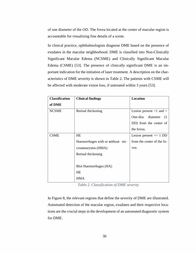
In clinical practice, ophthalmologists diagnose DME based on the presence of
exudates in the macular neighborhood. DME is classified into Non-Clinically
Significant Macular Edema (NCSME) and Clinically Significant Macular
Edema (CSME) [53]. The presence of clinically significant DME is an im-
portant indication for the initiation of laser treatment. A description on the char-
acteristics of DME severity is shown in Table 2. The patients with CSME will
be affected with moderate vision loss, if untreated within 3 years [53].
Classification
of DME
Clinical findings Location
NCSME Retinal thickening Lesion present >1 and >
One-disc diameter (1
DD) from the center of
the fovea.
CSME HE
Haemorrhages with or without mi-
croaneurysms (HMA)
Retinal thickening
Blot Haemorrhages (HA)
HE
HMA
Lesion present <= 1 DD
from the center of the fo-
vea.
Table 2. Classification of DME severity
In Figure 8, the relevant regions that define the severity of DME are illustrated.
Automated detection of the macular region, exudates and their respective loca-
tions are the crucial steps in the development of an automated diagnostic system
for DME.
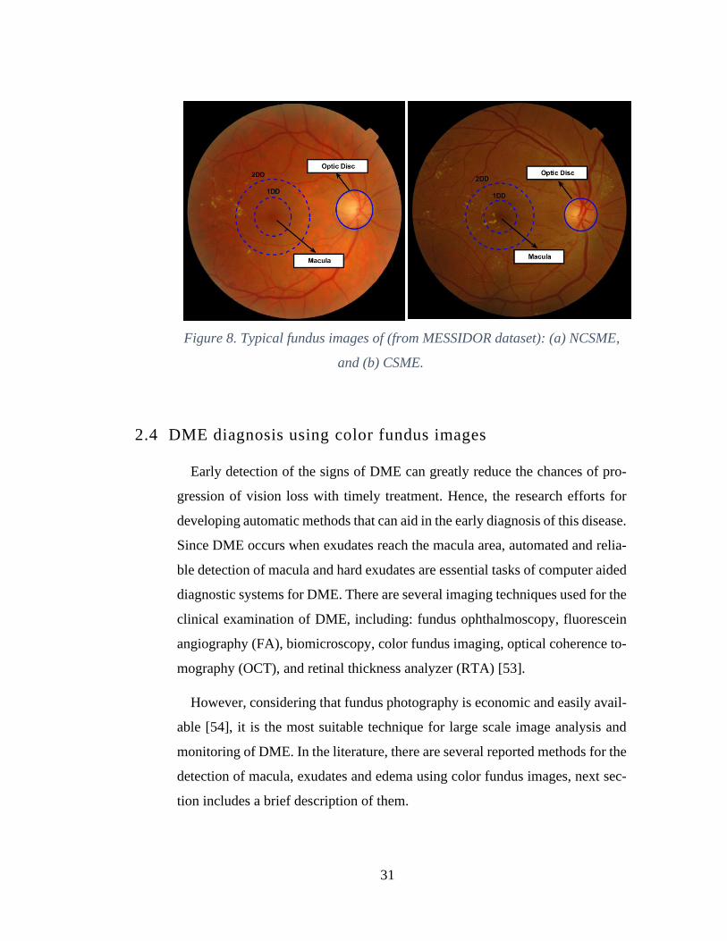
31
Figure 8. Typical fundus images of (from MESSIDOR dataset): (a) NCSME,
and (b) CSME.
2.4 DME diagnosis using color fundus images
Early detection of the signs of DME can greatly reduce the chances of pro-
gression of vision loss with timely treatment. Hence, the research efforts for
developing automatic methods that can aid in the early diagnosis of this disease.
Since DME occurs when exudates reach the macula area, automated and relia-
ble detection of macula and hard exudates are essential tasks of computer aided
diagnostic systems for DME. There are several imaging techniques used for the
clinical examination of DME, including: fundus ophthalmoscopy, fluorescein
angiography (FA), biomicroscopy, color fundus imaging, optical coherence to-
mography (OCT), and retinal thickness analyzer (RTA) [53].
However, considering that fundus photography is economic and easily avail-
able [54], it is the most suitable technique for large scale image analysis and
monitoring of DME. In the literature, there are several reported methods for the
detection of macula, exudates and edema using color fundus images, next sec-
tion includes a brief description of them.
32
2.4.1 Macula and fovea detection
In color fundus images, macula is identified as a darker object located on the
temporal side of the optic nerve head. Since the macula contains the highest
concentration of photoreceptors is responsible for visual acuity. Any damage in
macula region or presence of abnormalities like exudates, cotton wool spots and
red lesions could lead to loss of central vision. The progressive damage in the
macula or presence of hard exudates near to macular region is an eye disease
recognized as Clinically Significant Macular Edema (CSME).
Macula characteristics: The macula is a round area in the central region of
the retina, which measures about 3 to 4 mm in diameter [55] and is responsible
for central and high-resolution vision. In the fundus color images, macula can
be observed as a darker/red-brown color oval-shaped object located on the tem-
poral region of retina. An important characteristic of the macula region is that
is devoid of vessels. Located at the center of the macula, there is a small de-
pression that appears as a round dark area of approximately 1 mm of diameter,
called fovea. Anatomically, the center of the fovea is located at the range of 2
to 2.5 optic disc (OD) diameters on average from the OD center [55]. The fovea
radius is between one third and one fourth of the macula radius, and the macula
radius is approximately equal to one OD diameter.
However, macula detection is not an easy task, as the whole macula area is
not generally distinguishable in retinal color images. The contrast in the macu-
lar region is often low and it can be obscured by the presence of lesions, includ-
ing large clusters of hard exudates and/or hemorrhages. On the other hand, the
color and intensity of the macula varies greatly across individuals due to varia-
tions in the levels of pigment associated to factors such as ethnicity, diet, age
and disease conditions. Algorithms for macula detection often fail when there
is presence of large hemorrhages, as macula exhibits similar intensity/texture
of red lesions.
33
From the literature review, macula localization methods can be categorized
in three main groups: visual-based methods, positional constraints-based meth-
ods and hybrid methods.
Visual-based methods
In this category, there are included the approaches that attempt to find the
macula using exclusively the visual properties of the fovea, i.e. intensity, size,
shape and texture.
Akram et al. [56] approach consists of the detection of macula using a de-
tailed set of features and Gaussian mixtures model-based (GMM) classifier.
First, contrast enhancement on green channel is applied to improve the con-
trast of dark regions. Next, the binary map for possible macular region is
created from above contrast enhanced image by applying a low adaptive
threshold value. Blood vessels are extracted using the method reported on
[57] and subtracted, so that, only the dark candidate objects remain. Next step
is to extract for each candidate region a number of features. Finally, classifi-
cation is done by using GMM. The author reported an accuracy of 97.2% for
MESSIDOR dataset and 98.22% for HEIMED dataset.
Geetha et al. [58] proposed method avoids knowledge of other retinal
structures and attempts data mining techniques to segment macula. Unsuper-
vised clustering algorithm is used for this purpose. A heuristic based cluster-
ing in which initial centers are selected based on measures defining statistical
distribution of data is incorporated in the proposed methodology. The ap-
proach comprises three stages: image pre-processing, data mining and image
postprocessing. The pre-processing stage includes image cropping, green
channel extraction, contrast enhancement using CLAHE and application of
mathematical closing. Next, the pre-processed image is subjected to heuristic
based clustering yielding a binary map. The binary image is post-processed

34
to eliminate unwanted components. Finally, the component which possessed
the minimum intensity is determined as macula and its center constitutes the
fovea. The authors reported accuracies following the 1R criterion of 100%,
100%, 96.92%, 97.75% 98.81%, 90% and 99.33% for HRF, DRIVE, DI-
ARETDB0, DIARETDB1, HEI-MED, STARE and MESSIDOR, respec-
tively.
Positional constraints-based methods
Positional constraint-based methods to locate the macula rely on obtaining an
estimation of the fovea center location making use of its known anatomical
features regarding its position on the retinal surface i.e. approximate distance
from OD and the absence of vessels.
Kao et al. [59] proposed method, comprises four stages. In the first step, the
fundus image is processed to find the region-of-interest excluding the dark
areas around the fundus image. In the second step, the optic disc center is
localized using a template matching method. In the third step, the disc–fovea
axis (a line connecting the optic disc center and the fovea) is determined,
based on the vessel-free region. Finally, the fovea center is located around
the center of the disc–fovea axis by matching the fovea template around the
center of the axis. Adaptive Gaussian templates were used to localize the cen-
ters of the optic disc and fovea for the images with different resolutions. The
authors reported accuracy values of 93.1%, 92.1% and 97.8% for the DI-
ARETDB0, DIARETDB1 and MESSIDOR databases, respectively.
Deka et al. [60] approach for macula detection consists in investigating the
structure of blood vessels (BV) in the macular region. Macula localization
process consists of pre-processing using CLAHE and detection of blood
35
vessels. For detection of BV 5th order Discrete Wavelet Transform (DWT)
decomposition and morphological opening operation is applied. Next, using
property of BV structure where the macula neighborhood is lack of BV
whereas, maximum number BV present in the neighborhood of OD, a ROI
that contains the macula is selected. Finally, the BV are removed from the
ROI using morphological closing operation, the image is inverted and region
growing is applied to segment out the macula region. The authors reported
an accuracy 100%, 97.75%, 95.5%, 100%, and 96% for DRIVE, MESSI-
DOR, DIARETDB1, HRF, STARE datasets, respectively.
Hybrid methods
In this category are the methods that combine visual and positional con-
straint-based methods with the aim of exploiting the benefits of both tech-
niques.
Aquino et al. [55] method comprises first, on an acceptable fovea center es-
timation by using a priori known anatomical features with respect to the optic
disc and the vascular tree. For this purpose, the line delimiting the superior
and inferior vessels defined as raphe is located using the method reported on
[61], [62] and the fovea center is assumed to reside at a fixed distance along
this line at 2.5 OD diameters from the OD center. Second, a morphological
processing is employed to improve the obtained fovea center estimation when
the fovea is detectable in the image; otherwise, it is declared indistinguishable
and the first result is retained. The methodology was tested on the MESSI-
DOR and DIARETDB1 databases using of a distance criterion between the
obtained and the real fovea center. Fovea center in the brackets between the
categories Excellent and Fair (fovea centers primarily accepted as valid in the
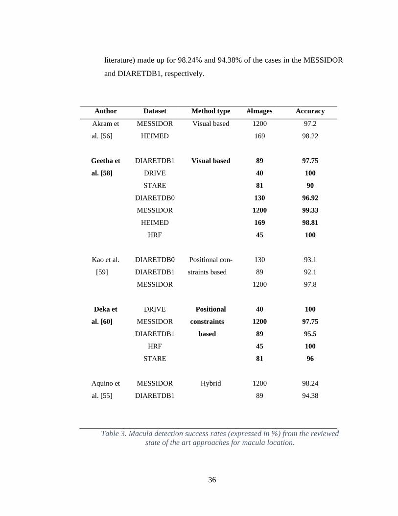
36
literature) made up for 98.24% and 94.38% of the cases in the MESSIDOR
and DIARETDB1, respectively.
Author Dataset Method type #Images Accuracy
Akram et
al. [56]
MESSIDOR
HEIMED
Visual based 1200
169
97.2
98.22
Geetha et
al. [58]
Kao et al.
[59]
Deka et
al. [60]
Aquino et
al. [55]
DIARETDB1
DRIVE
STARE
DIARETDB0
MESSIDOR
HEIMED
HRF
DIARETDB0
DIARETDB1
MESSIDOR
DRIVE
MESSIDOR
DIARETDB1
HRF
STARE
MESSIDOR
DIARETDB1
Visual based
Positional con-
straints based
Positional
constraints
based
Hybrid
89
40
81
130
1200
169
45
130
89
1200
40
1200
89
45
81
1200
89
97.75
100
90
96.92
99.33
98.81
100
93.1
92.1
97.8
100
97.75
95.5
100
96
98.24
94.38
Table 3. Macula detection success rates (expressed in %) from the reviewed
state of the art approaches for macula location.

37
Table 3 shows the summary of the reviewed macula location approaches. The
methods marked in bold correspond to the best performing, taking into account
the accuracy rate and the number of datasets considered.
2.4.2. Exudate segmentation
Exudates are constituted by the yellow deposits that leak from the blood
vessels onto the posterior pole of the fundus image, these lesions are devel-
oped in diabetic patients when diabetes has remained uncontrolled a long
time. Exudate detection acts as a marker in diagnosing DME.
Exudates characteristics: Exudates are yellow-white lesions with relatively
distinctive borders. The exudates consist of lipids and proteins that flow from
the damaged blood vessels of the retina. They appear as bright patterns and
their contrast is high compared to the background. From a visual inspection,
the exudates appear indistinctly yellowish with different sizes, shapes and
locations, as shown in Figure 9. They are usually seen in bands, groups or in
large circular structures.
(a)
(b)
Figure 9. (a) Circular cluster of hard exudates. (b) Flame-shaped hard
exudates.
38
The segmentation methods for exudates, can be categorized in five groups:
thresholding-based; morphology-based; region growing-based; supervised; and
hybrid.
Thresholding based methods
Thresholding approaches employ local and global gray-level analysis to seg-
ment retinal exudates. Exudates have higher gray level compared to the nearby
retinal background in the green component. Due to significant gray level change
(shadows and poor illumination) in the whole image. It is quite difficult to find
a global threshold that distinguishes the exudates from the background. There-
fore, a local threshold is calculated for sub-windows of the fundus image, per
its local histogram.
Garaibeh et al. [63] assumed that the color mode for image is bimodal where
the number of pixels belongs to the background is much higher than the pixels
that belong to exudates. A benefit from this feature is that the mean of the whole
image is closer to the mean of the pixel that belongs to background. Then, sub-
tracting, the mean of the whole image from the image will produce an image
that mainly contains exudates. Then, they removed the noise using median fil-
ter. After that, a thresholding technique was applied to separate exudate pixels
from others. A sensitivity of 92.1% was reported on DIARETDB0 dataset.
Reza et al. [64] proposed method made use of: preprocessing algorithms to
make the bright object features more distinguishable from the background,
markers to modify the gradient image that control over-segmentation and wa-
tershed segmentation to trace the boundary from the marker modified gradient.
The advantages of the proposed method are: there is no need to select different
threshold value for different test images those of which are varying with differ-
ent brightness and contrast conditions (the method proposed in this study only
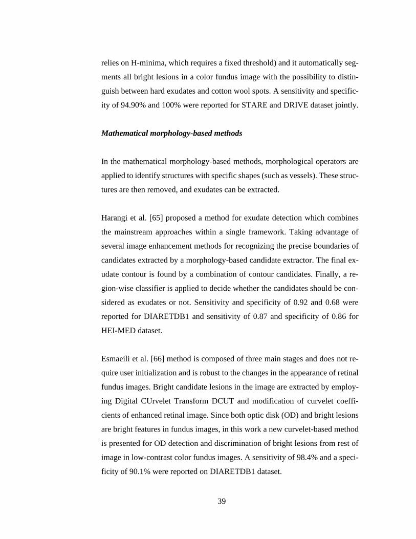
39
relies on H-minima, which requires a fixed threshold) and it automatically seg-
ments all bright lesions in a color fundus image with the possibility to distin-
guish between hard exudates and cotton wool spots. A sensitivity and specific-
ity of 94.90% and 100% were reported for STARE and DRIVE dataset jointly.
Mathematical morphology-based methods
In the mathematical morphology-based methods, morphological operators are
applied to identify structures with specific shapes (such as vessels). These struc-
tures are then removed, and exudates can be extracted.
Harangi et al. [65] proposed a method for exudate detection which combines
the mainstream approaches within a single framework. Taking advantage of
several image enhancement methods for recognizing the precise boundaries of
candidates extracted by a morphology-based candidate extractor. The final ex-
udate contour is found by a combination of contour candidates. Finally, a re-
gion-wise classifier is applied to decide whether the candidates should be con-
sidered as exudates or not. Sensitivity and specificity of 0.92 and 0.68 were
reported for DIARETDB1 and sensitivity of 0.87 and specificity of 0.86 for
HEI-MED dataset.
Esmaeili et al. [66] method is composed of three main stages and does not re-
quire user initialization and is robust to the changes in the appearance of retinal
fundus images. Bright candidate lesions in the image are extracted by employ-
ing Digital CUrvelet Transform DCUT and modification of curvelet coeffi-
cients of enhanced retinal image. Since both optic disk (OD) and bright lesions
are bright features in fundus images, in this work a new curvelet-based method
is presented for OD detection and discrimination of bright lesions from rest of
image in low-contrast color fundus images. A sensitivity of 98.4% and a speci-
ficity of 90.1% were reported on DIARETDB1 dataset.

40
Akram et al. [67] approach consists in generating a feature set for each region
depending upon their shape, gray level, color and statistical based properties.
The true MA regions are selected and classified using a hybrid classifier which
is a weighted combination of multivariate m-Mediods, GMM and SVM. The
main contribution of this work is that it improves the accuracies of all three
stages using accurate vascular segmentation, sound feature set and hybrid clas-
sifier for accurate detection of MAs. The proposed method introduces the elim-
ination of blood vessel pixels prior to MAs detection and enhances the feature
space before applying the classifier. A sensitivity and specificity of 98.64% and
99.69% were reported for DIARETDB1 and DIARETDB0 datasets jointly.
Region growing based methods
For region growing based methods, spatial gray-level contiguity features are
employed for retinal exudate segmentation. This segmentation approach exam-
ines neighboring pixels of initial seed points and determines whether the neigh-
bor pixels should be added to the region.
Pereira et al. [68] applied a new approach for segmenting exudates based on
Ant Colony Optimization (ACO). ACO is a branch of a larger field referred to
as swarm intelligence and it is inspired by observation of the collective foraging
behavior of real ant colonies. Using artificial ant colonies, the problem solutions
are constructed within a stochastic iterative process by adding solution compo-
nents to partial solutions. Each ant constructs a part of the solution using artifi-
cial pheromone, which reflects the ant's accumulated experience and heuristic
information depending on the problem. A sensitivity of 0.80 and a specificity
of 0.99 were reported on HEI-MED dataset.
41
Supervised methods
Supervised methods are literature’s most frequent works. A feature vector is
constructed for each pixel or pixel cluster, to be classified with a machine learn-
ing approach into exudates or non-exudates. The features are based on the color
(typically gray level in green channel), brightness, size, shape, edge strength,
texture, and contextual information of pixel clusters. Among the most frequent
machine learning approaches are: neural networks [69], support vector ma-
chines (SVMs) [70], [71], [72], and the Naïve Bayes classifier [73].
Bhargavi et al. [70] used a combination of existing techniques in order to
achieve better sensitivity, specificity and accuracy. The bilateral filtering is ap-
plied as a preprocessing step, contrast enhancement is done to increase the con-
trast between foreground with exudates and background elements like optic
disk and vessels. To characterize the segmented lesions, texture features are
used. Finally, they use a support vector machine classifier to distinguish the
lesions and non-lesions images. 20 features are used for SVM classifier. A sen-
sitivity and specificity of 100% and 94.6% were reported for DIARETDB1 and
MESSIDOR datasets jointly.
Akram et al. [73] proposed a method for detection and classification of exudates
in colored retinal images. The novel technique uses filter banks to extract the
candidate regions for possible exudates. It eliminates the spurious exudate re-
gions by removing the optic disc region. Then it applies a Bayesian classifier as
a combination of Gaussian functions to detect exudate and non-exudate regions.
Sensitivities of 99.5%, 97.72%, 93.7% and specificities of 98.35%, 96.15%,
98.38% were reported on DIARETDB1, STARE and DIARETDB0 datasets re-
spectively.
42
Hybrid methods
This group correspond to segmentation methods that don’t rely only on the le-
sions’ properties (color, shape, size), matching a template or applying super-
vised learning only. Instead they combine two or more of the above methods.
Liu et al. [74] presented a location-to-segmentation strategy for exudate seg-
mentation, with three stages: anatomic structures removal stage, exudate loca-
tion stage and exudate segmentation stage. To describe the local texture struc-
tures of the exudate regions, the histogram of CLBP (Cluster Local Binary Pat-
terns) is used, in which both the local difference sign and magnitude between
the exudate pixel and neighboring background pixels are considered. An exu-
date region segmentation method from the located patches is proposed. Because
the patches include both exudate regions and background regions and there ex-
ists high contrast between them, size is exploited prior and regional contrast
prior about the exudate regions for segmentation. A sensitivity of 83% and a
specificity of 75% were reported on DIARETDB1 dataset and a sensitivity of
76% on E-ophtha dataset.
Imani et al. [64] proposed a method for exudate detection based on Morpholog-
ical Component Analysis (MCA) algorithm. This algorithm offers a signal sep-
aration method which utilizes sparsity property to separate the sources. The
MCA was utilized to separate vessels from lesions in the retinal images for a
separate analysis. By cleaning the retinal images, exudate lesions are easily seg-
mented using dynamic thresholding and mathematical morphology. Sensitivi-
ties of 89.01%, 80.32% and specificities of 99.93%, 99.83% were reported on
DIARETDB1, and E-ophtha datasets respectively.

43
Author Dataset Method type #Images Sensitivity/
Specificity
Garaibeh
et al. [63]
DIARETDB0
Thresholding
based
130
92.1 / -
Reza et
al. [64]
Harangi
et al. [65]
Esmaeili
et al. [66]
Akram et
al. [67]
Pereira et
al. [68]
Bhargavi
et al. [70]
Akram et
al. [73]
Liu et al.
[74]
STARE
DRIVE
DIARETDB1
HEIMED
DIARETDB1
DIARETDB1
DIARETDB0
HEIMED
DIARETDB1
MESSIDOR
DIARETDB1
STARE
DIARETDB0
DIARETDB1
e-ophtha-EX
Thresholding
based
Mathematical
morphology-
based
Mathematical
morphology-
based
Mathematical
morphology-
based
Region grow-
ing based
Supervised
Supervised
Hybrid
81
40
89
169
89
89
130
169
89
1200
89
81
130
89
82
94.9 / 100
jointly
92 / 68
87 / 86
98.4 / 90.1
98.64 / 99.69
jointly
80 / 99
100 / 94.6
jointly
99.5 / 98.35
97.72 / 96.15
93.7 / 98.38
83 / 75
76 / -
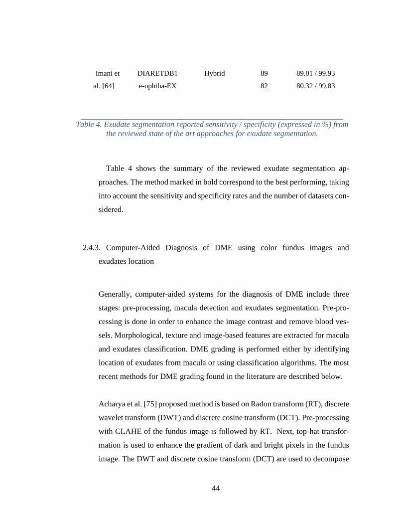
44
Imani et
al. [64]
DIARETDB1
e-ophtha-EX
Hybrid
89
82
89.01 / 99.93
80.32 / 99.83
Table 4. Exudate segmentation reported sensitivity / specificity (expressed in %) from
the reviewed state of the art approaches for exudate segmentation.
Table 4 shows the summary of the reviewed exudate segmentation ap-
proaches. The method marked in bold correspond to the best performing, taking
into account the sensitivity and specificity rates and the number of datasets con-
sidered.
2.4.3. Computer-Aided Diagnosis of DME using color fundus images and
exudates location
Generally, computer-aided systems for the diagnosis of DME include three
stages: pre-processing, macula detection and exudates segmentation. Pre-pro-
cessing is done in order to enhance the image contrast and remove blood ves-
sels. Morphological, texture and image-based features are extracted for macula
and exudates classification. DME grading is performed either by identifying
location of exudates from macula or using classification algorithms. The most
recent methods for DME grading found in the literature are described below.
Acharya et al. [75] proposed method is based on Radon transform (RT), discrete
wavelet transform (DWT) and discrete cosine transform (DCT). Pre-processing
with CLAHE of the fundus image is followed by RT. Next, top-hat transfor-
mation is used to enhance the gradient of dark and bright pixels in the fundus
image. The DWT and discrete cosine transform (DCT) are used to decompose
45
the sinogram image into various frequency coefficients. These coefficients are
converted into 1D vector by arranging the coefficients in zig-zag manner. This
1D signal is subjected to locality sensitive discriminant analysis (LSDA). Fi-
nally, four supervised classifiers: decision tree (Dt), K-nearest neighbor (K-nn),
Probabilistic neural network (Pnn) and Support Vector Machine (SVM) are
used to classify the three classes normal, NCSME and CSME using significant
features. The authors reported an accuracy of 97.01%, 88% and 94.16% for
normal, NCSME and CSME cases, respectively.
Medhi et al. [76] proposed approach is implemented in two stages. The first
stage involves preprocessing where illumination correction is applied to the in-
put image and resizing to 768x576 resolution; next, the optic disc is masked to
avoid false detection during bright lesion identification. The second stage com-
prises DME detection and its analysis. Here, the retinal lesions including mi-
croaneurysms, hemorrhages and exudates are identified by applying mathemat-
ical morphology processing to the green and hue plane color images. The mac-
ula and the fovea locations are determined using intensity property of processed
red plane image. Different circular regions are thereafter marked in the neigh-
borhood of the macula. The presence of lesions in these regions is identified to
confirm positive maculopathy. Later, the information is used for evaluating its
severity. The authors reported and average accuracy of 98.86% and an average
specificity of 98.05% for DRIVE, Diaretdb1, MESSIDOR and HRF publicly
available datasets altogether.
Marin et al. [77] proposed methodology consists in applying digital image pro-
cessing algorithms to the retinal image in order to obtain a set of candidate re-
gions to be Exudate (Ex), which are validated by means of feature extraction
and supervised classification techniques. First, the fundus image is pre-pro-
cessed for background homogenization, green channel pixels are corrected ac-
cording to intensity and contrast values that are representative of the
46
background in its neighborhood, these values are estimated by mean and local
standard deviation. Next, and adaptive noise-removal filtering is applied. The
filter works with a small-sized neighborhood and a noise variance, set to the
statistical mode of the local variance values. For candidate generation of exu-
dates, adaptative global thresholding is applied. Optic disc is extracted using
the methodology described in [37] to avoid false positives. Finally, a supervised
classification process using a regularized local regression is applied to detect
those regions considered as actual exudates. The features include, color and
edge strength-based features and features based on responses from Gaussian
and Difference of Gaussian (DoG) filter bank. The author reported a sensitivity
of 90% and a specificity of 69.39% for MESSIDOR dataset.
Akram et al [56] proposed approach consists of a novel method for accurate
detection of macula using a detailed feature set and Gaussian mixtures model-
based classifier. The method consists of three phases: exudate detection, macula
detection and grading of DME. In first phase, the all possible regions which
may be considered as exudates are extracted and represented with a number of
features. Morphological closing is applied to the fundus image to remove the
effect of blood vessels and dark lesions. Next, an adaptive contrast enhance-
ment technique [78] is applied, followed by the convolution with a filter bank
based on Gabor kernel. Following, a binary map containing candidate exudate
regions by applying adaptive threshold value using Otsu algorithm and then the
OD is detected using averaging and Hough transform given in [79]. The features
extracted for each candidate exudate region are: area, compactness, mean green
channel intensity, mean hue, mean gradient magnitude, entropy, energy and
third moment. Exudates are classified using a hybrid classifier combining
GMM and SVM. In second phase, macula detection is performed by generating
a detailed set of features and Gaussian mixtures model-based (GMM) classifier.
In last phase, macular coordinates and location of exudates are used to grade
the input image in one of the two stages of edema: Non CSME and CSME. The
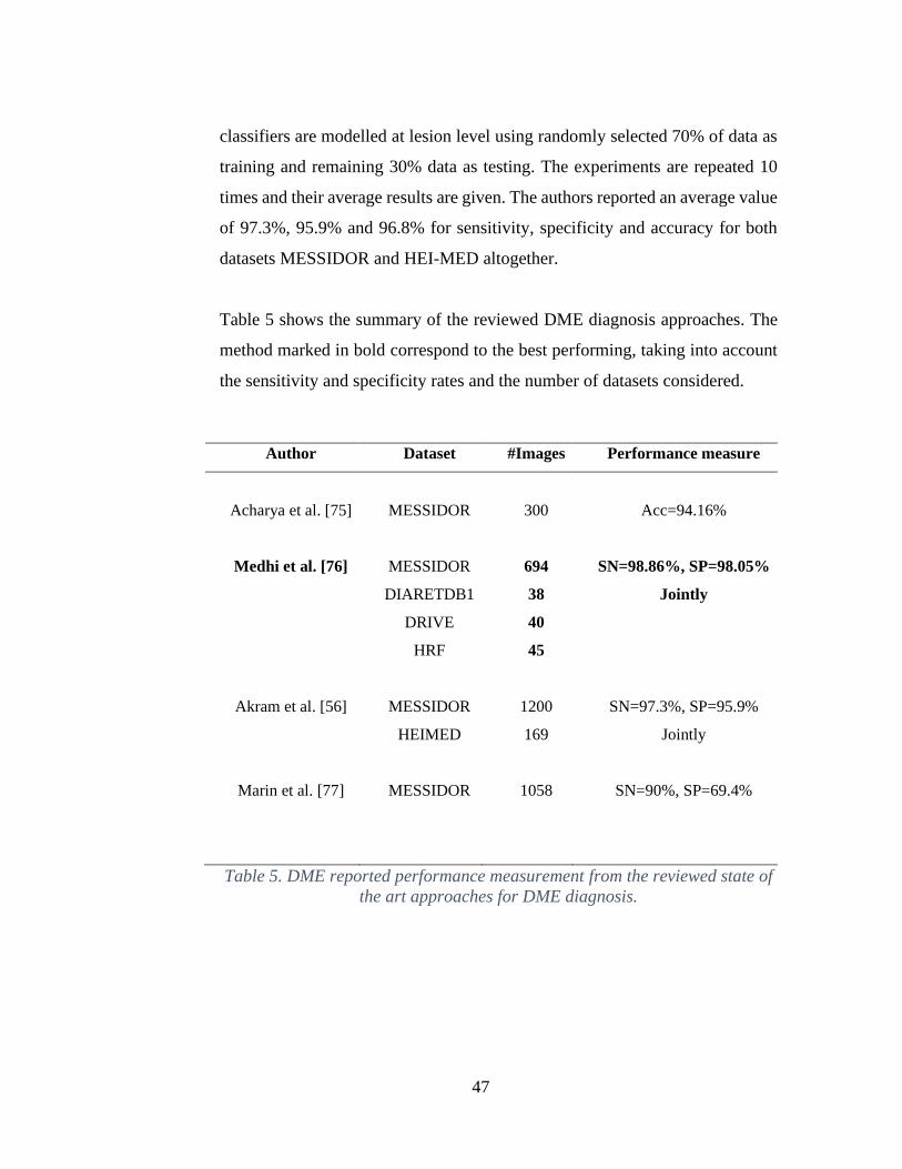
47
classifiers are modelled at lesion level using randomly selected 70% of data as
training and remaining 30% data as testing. The experiments are repeated 10
times and their average results are given. The authors reported an average value
of 97.3%, 95.9% and 96.8% for sensitivity, specificity and accuracy for both
datasets MESSIDOR and HEI-MED altogether.
Table 5 shows the summary of the reviewed DME diagnosis approaches. The
method marked in bold correspond to the best performing, taking into account
the sensitivity and specificity rates and the number of datasets considered.
Author Dataset #Images Performance measure
Acharya et al. [75] MESSIDOR
300
Acc=94.16%
Medhi et al. [76]
Akram et al. [56]
Marin et al. [77]
MESSIDOR
DIARETDB1
DRIVE
HRF
MESSIDOR
HEIMED
MESSIDOR
694
38
40
45
1200
169
1058
SN=98.86%, SP=98.05%
Jointly
SN=97.3%, SP=95.9%
Jointly
SN=90%, SP=69.4%
Table 5. DME reported performance measurement from the reviewed state of
the art approaches for DME diagnosis.
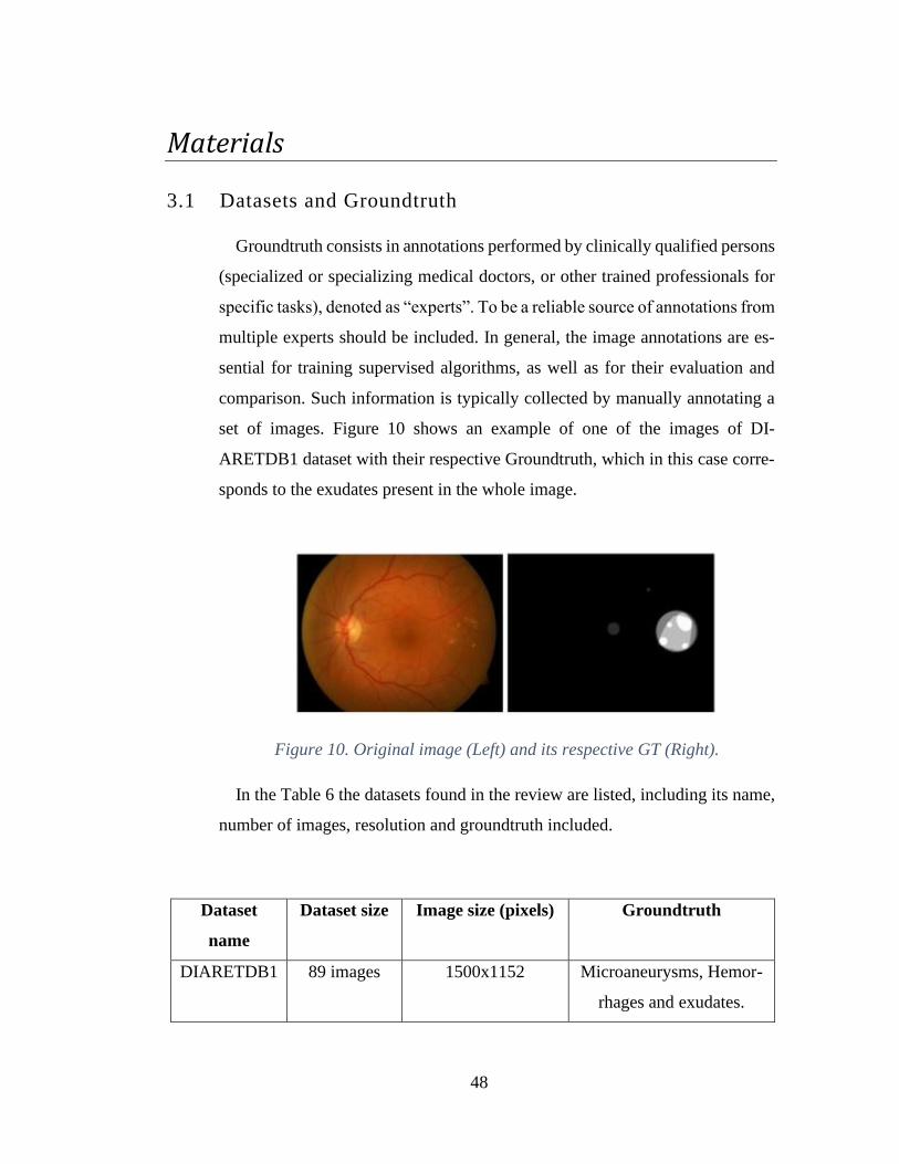
48
Materials
3.1 Datasets and Groundtruth
Groundtruth consists in annotations performed by clinically qualified persons
(specialized or specializing medical doctors, or other trained professionals for
specific tasks), denoted as “experts”. To be a reliable source of annotations from
multiple experts should be included. In general, the image annotations are es-
sential for training supervised algorithms, as well as for their evaluation and
comparison. Such information is typically collected by manually annotating a
set of images. Figure 10 shows an example of one of the images of DI-
ARETDB1 dataset with their respective Groundtruth, which in this case corre-
sponds to the exudates present in the whole image.
Figure 10. Original image (Left) and its respective GT (Right).
In the Table 6 the datasets found in the review are listed, including its name,
number of images, resolution and groundtruth included.
Dataset
name
Dataset size Image size (pixels) Groundtruth
DIARETDB1 89 images 1500x1152 Microaneurysms, Hemor-
rhages and exudates.
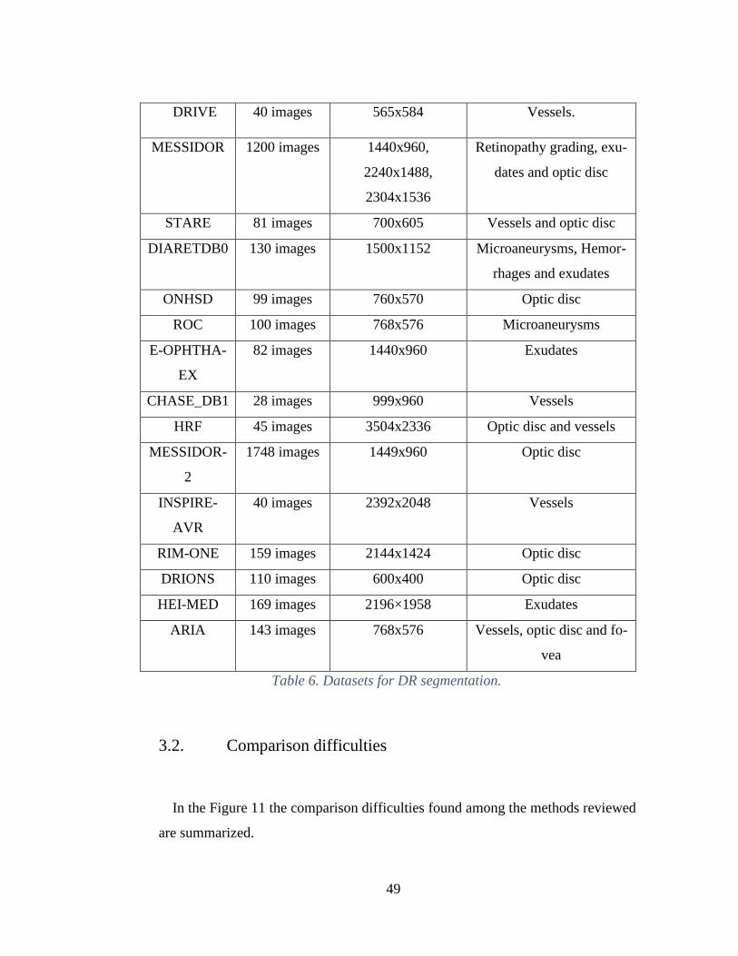
49
DRIVE 40 images 565x584 Vessels.
MESSIDOR 1200 images 1440x960,
2240x1488,
2304x1536
Retinopathy grading, exu-
dates and optic disc
STARE 81 images 700x605 Vessels and optic disc
DIARETDB0 130 images 1500x1152 Microaneurysms, Hemor-
rhages and exudates
ONHSD 99 images 760x570 Optic disc
ROC 100 images 768x576 Microaneurysms
E-OPHTHA-
EX
82 images 1440x960 Exudates
CHASE_DB1 28 images 999x960 Vessels
HRF 45 images 3504x2336 Optic disc and vessels
MESSIDOR-
2
1748 images 1449x960 Optic disc
INSPIRE-
AVR
40 images 2392x2048 Vessels
RIM-ONE 159 images 2144x1424 Optic disc
DRIONS 110 images 600x400 Optic disc
HEI-MED 169 images 2196×1958 Exudates
ARIA 143 images 768x576 Vessels, optic disc and fo-
vea
Table 6. Datasets for DR segmentation.
3.2. Comparison difficulties
In the Figure 11 the comparison difficulties found among the methods reviewed
are summarized.
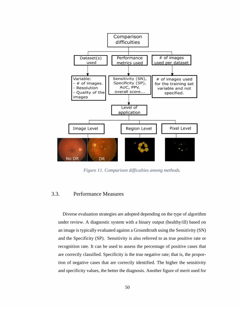
50
Figure 11. Comparison difficulties among methods.
3.3. Performance Measures
Diverse evaluation strategies are adopted depending on the type of algorithm
under review. A diagnostic system with a binary output (healthy/ill) based on
an image is typically evaluated against a Groundtruth using the Sensitivity (SN)
and the Specificity (SP). Sensitivity is also referred to as true positive rate or
recognition rate. It can be used to assess the percentage of positive cases that
are correctly classified. Specificity is the true negative rate; that is, the propor-
tion of negative cases that are correctly identified. The higher the sensitivity
and specificity values, the better the diagnosis. Another figure of merit used for
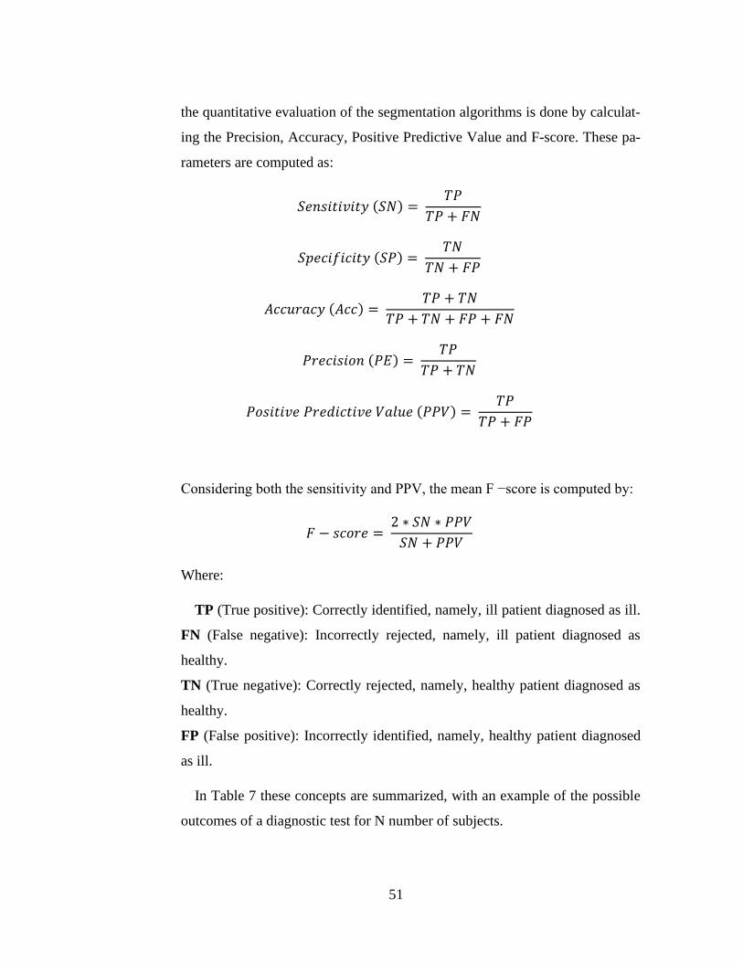
51
the quantitative evaluation of the segmentation algorithms is done by calculat-
ing the Precision, Accuracy, Positive Predictive Value and F-score. These pa-
rameters are computed as:
𝑆𝑒𝑛𝑠𝑖𝑡𝑖𝑣𝑖𝑡𝑦 (𝑆𝑁) = 𝑇𝑃
𝑇𝑃 + 𝐹𝑁
𝑆𝑝𝑒𝑐𝑖𝑓𝑖𝑐𝑖𝑡𝑦 (𝑆𝑃) = 𝑇𝑁
𝑇𝑁 + 𝐹𝑃
𝐴𝑐𝑐𝑢𝑟𝑎𝑐𝑦 (𝐴𝑐𝑐) = 𝑇𝑃 + 𝑇𝑁
𝑇𝑃 + 𝑇𝑁 + 𝐹𝑃 + 𝐹𝑁
𝑃𝑟𝑒𝑐𝑖𝑠𝑖𝑜𝑛 (𝑃𝐸) = 𝑇𝑃
𝑇𝑃 + 𝑇𝑁
𝑃𝑜𝑠𝑖𝑡𝑖𝑣𝑒 𝑃𝑟𝑒𝑑𝑖𝑐𝑡𝑖𝑣𝑒 𝑉𝑎𝑙𝑢𝑒 (𝑃𝑃𝑉) = 𝑇𝑃
𝑇𝑃 + 𝐹𝑃
Considering both the sensitivity and PPV, the mean F −score is computed by:
𝐹 − 𝑠𝑐𝑜𝑟𝑒 = 2 ∗ 𝑆𝑁 ∗ 𝑃𝑃𝑉
𝑆𝑁 + 𝑃𝑃𝑉
Where:
TP (True positive): Correctly identified, namely, ill patient diagnosed as ill.
FN (False negative): Incorrectly rejected, namely, ill patient diagnosed as
healthy.
TN (True negative): Correctly rejected, namely, healthy patient diagnosed as
healthy.
FP (False positive): Incorrectly identified, namely, healthy patient diagnosed
as ill.
In Table 7 these concepts are summarized, with an example of the possible
outcomes of a diagnostic test for N number of subjects.
52
True clinical status ac-
cording to GT
Total
Abnormal Normal
Re-
sult of
the di-
agnostic
test
Ab-
nor-
mal
True posi-
tives (TP)
False posi-
tives (FP)
Abnormal= TP +
FP
Nor-
mal
False nega-
tives (FN)
True nega-
tives (TN)
Normal= TN + FN
To-
tal
Abnormal
cases = TP +
FN
Normal
cases= FP +
TN
TP+FN+FP+TN=N
Table 7. example of the possible outcomes of a diagnostic test for N number of
subjects.
Sensitivity in essence, measures how good an analysis is in finding any anom-
aly, if it exists, represents the actual proportion of positives that are correctly
identified. Specificity is a measure against false positives, showing how reliable
an analysis is, representing the proportion of negatives that are correctly iden-
tified. Since sensitivity is a more significant measure than specificity, most re-
searchers propose highly sensitive schemes for the detection of DR [80].
Nevertheless, the majority of researches found in the literature use some of
the figures of merit previously exposed, still is difficult to directly compare
them. That is because, sensitivity and specificity can be applied at different lev-
els:
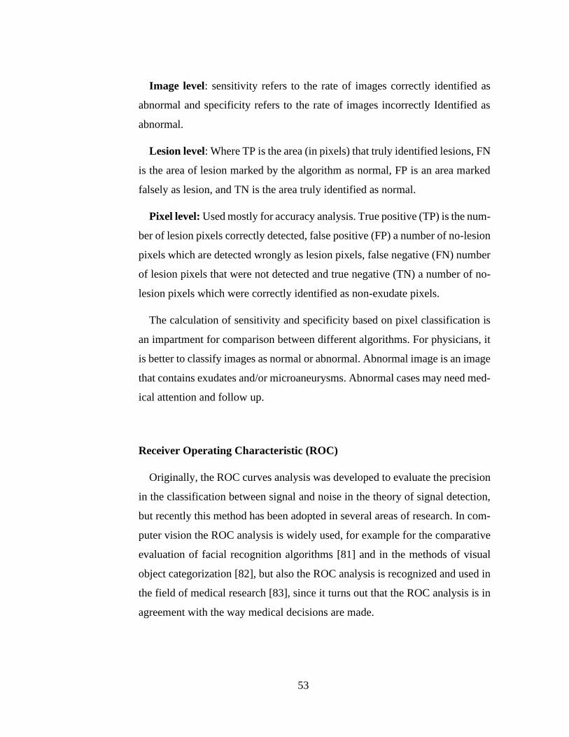
53
Image level: sensitivity refers to the rate of images correctly identified as
abnormal and specificity refers to the rate of images incorrectly Identified as
abnormal.
Lesion level: Where TP is the area (in pixels) that truly identified lesions, FN
is the area of lesion marked by the algorithm as normal, FP is an area marked
falsely as lesion, and TN is the area truly identified as normal.
Pixel level: Used mostly for accuracy analysis. True positive (TP) is the num-
ber of lesion pixels correctly detected, false positive (FP) a number of no-lesion
pixels which are detected wrongly as lesion pixels, false negative (FN) number
of lesion pixels that were not detected and true negative (TN) a number of no-
lesion pixels which were correctly identified as non-exudate pixels.
The calculation of sensitivity and specificity based on pixel classification is
an impartment for comparison between different algorithms. For physicians, it
is better to classify images as normal or abnormal. Abnormal image is an image
that contains exudates and/or microaneurysms. Abnormal cases may need med-
ical attention and follow up.
Receiver Operating Characteristic (ROC)
Originally, the ROC curves analysis was developed to evaluate the precision
in the classification between signal and noise in the theory of signal detection,
but recently this method has been adopted in several areas of research. In com-
puter vision the ROC analysis is widely used, for example for the comparative
evaluation of facial recognition algorithms [81] and in the methods of visual
object categorization [82], but also the ROC analysis is recognized and used in
the field of medical research [83], since it turns out that the ROC analysis is in
agreement with the way medical decisions are made.
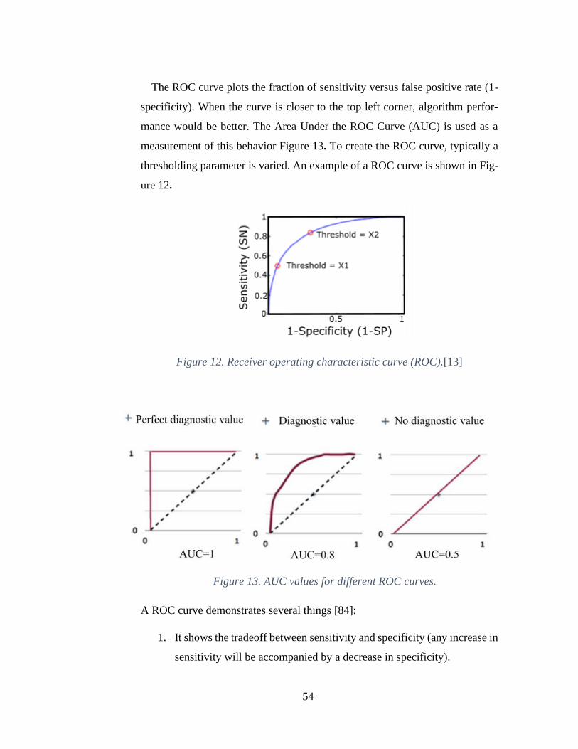
54
The ROC curve plots the fraction of sensitivity versus false positive rate (1-
specificity). When the curve is closer to the top left corner, algorithm perfor-
mance would be better. The Area Under the ROC Curve (AUC) is used as a
measurement of this behavior Figure 13. To create the ROC curve, typically a
thresholding parameter is varied. An example of a ROC curve is shown in Fig-
ure 12.
Figure 12. Receiver operating characteristic curve (ROC).[13]
Figure 13. AUC values for different ROC curves.
A ROC curve demonstrates several things [84]:
1. It shows the tradeoff between sensitivity and specificity (any increase in
sensitivity will be accompanied by a decrease in specificity).

55
2. The closer the curve follows the left-hand border and then the top border
of the ROC space, the more accurate the test.
3. The closer the curve comes to the 45-degree diagonal of the ROC space,
the less accurate the test.
4. The area under the curve is a measure of test accuracy.
Free-Response ROC Curve (FROC)
Region based analysis can be summarized using Free Response Operating
Characteristic (FROC) curves. This is similar to ROC analysis, except that the
false positive rate on the x-axis is replaced by the number of false positives per
image. In this case a definition of a detected region is needed and a typical ap-
proach expects a 50% overlap between the annotated and detected regions to
indicate a true positive.
Error function (Err2) (for Optic Disc only)
𝐸𝑟𝑟2 =1
𝑇𝑃 ∑ 𝑑((𝑥𝑟𝑒𝑠, 𝑦𝑟𝑒𝑠), (𝑥𝑚𝑎𝑛, 𝑦𝑚𝑎𝑛))(𝑥𝑟𝑒𝑠,𝑦𝑟𝑒𝑠) ∈ 𝑂𝐷𝑅
Where 𝑑((𝑥𝑟𝑒𝑠, 𝑦𝑟𝑒𝑠), (𝑥𝑚𝑎𝑛, 𝑦𝑚𝑎𝑛)) is the Euclidean distance of the detected
OD center (𝑥𝑟𝑒𝑠, 𝑦𝑟𝑒𝑠) and the manually given OD one (𝑥𝑚𝑎𝑛, 𝑦𝑚𝑎𝑛).
Oratio (for Optic Disc only)
𝑂𝑟𝑎𝑡𝑖𝑜 = 𝑇𝑃
𝑇𝑃 + 𝐹𝑃 + 𝐹𝑁
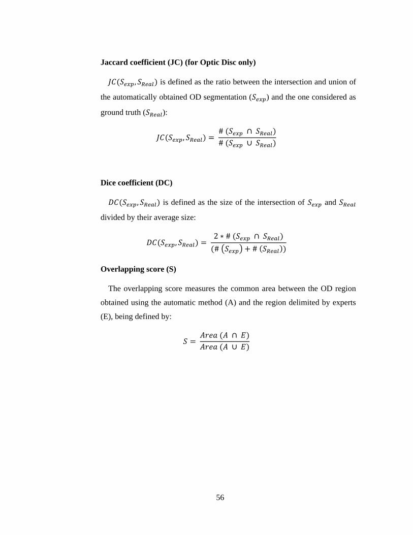
56
Jaccard coefficient (JC) (for Optic Disc only)
𝐽𝐶(𝑆𝑒𝑥𝑝, 𝑆𝑅𝑒𝑎𝑙) is defined as the ratio between the intersection and union of
the automatically obtained OD segmentation (𝑆𝑒𝑥𝑝) and the one considered as
ground truth (𝑆𝑅𝑒𝑎𝑙):
𝐽𝐶(𝑆𝑒𝑥𝑝, 𝑆𝑅𝑒𝑎𝑙) = # (𝑆𝑒𝑥𝑝 ∩ 𝑆𝑅𝑒𝑎𝑙)
# (𝑆𝑒𝑥𝑝 ∪ 𝑆𝑅𝑒𝑎𝑙)
Dice coefficient (DC)
𝐷𝐶(𝑆𝑒𝑥𝑝, 𝑆𝑅𝑒𝑎𝑙) is defined as the size of the intersection of 𝑆𝑒𝑥𝑝 and 𝑆𝑅𝑒𝑎𝑙
divided by their average size:
𝐷𝐶(𝑆𝑒𝑥𝑝, 𝑆𝑅𝑒𝑎𝑙) = 2 ∗ # (𝑆𝑒𝑥𝑝 ∩ 𝑆𝑅𝑒𝑎𝑙)
(# (𝑆𝑒𝑥𝑝) + # (𝑆𝑅𝑒𝑎𝑙))
Overlapping score (S)
The overlapping score measures the common area between the OD region
obtained using the automatic method (A) and the region delimited by experts
(E), being defined by:
𝑆 = 𝐴𝑟𝑒𝑎 (𝐴 ∩ 𝐸)
𝐴𝑟𝑒𝑎 (𝐴 ∪ 𝐸)
57
Methods
4.1 Optic disc Location
The location of the different normal ocular fundus structures such as: blood
vessels, optic disc, macula and fovea, is a common task within most of the au-
tomated detection systems for the detection of the early signs of retinopathy
diabetic and diabetic macular edema.
In particular, the location of the optic disc, which corresponds to the visible
part of the optic nerve in the eye, is an important task in systems dedicated to
the detection of exudates since the optic disc shares similar characteristics of
color and brightness, which can cause sections of it to be potentially erroneous
detected as exudates and therefore negatively affecting the system performance.
This can be avoided if OD correct location is known in advance. Additionally,
the state of the optical disc is important in diseases such as glaucoma, diabetic
optic neuropathy and other pathologies related to the optic nerve.
In the fundus image, the optic disc is characterized as a circular bright region
where the temporal and nasal veins emerge towards the eye, however, in retinal
images containing exudates, the brightest circular region could not correspond
always to the optic disc. For this reason, the methods that rely solely on finding
the brightest circular region or the bright region with the highest variation, only
present good performance in images of healthy retinas, but fail to correctly lo-
cate the optic disc in images containing exudates.
This chapter describes the proposed method for the optic disc location, in-
cluding a previous performance analysis of some thresholding techniques for
OD location in color fundus images, considering different image conditions and
the effect of applying a previous preprocessing technique on the segmentation
performance. The proposed OD location approach is based on OD’s character-
istic high intensity and a novel method for feature’s extraction which aims to
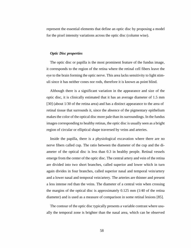
58
represent the essential elements that define an optic disc by proposing a model
for the pixel intensity variations across the optic disc (column wise).
Optic Disc properties
The optic disc or papilla is the most prominent feature of the fundus image,
it corresponds to the region of the retina where the retinal cell fibers leave the
eye to the brain forming the optic nerve. This area lacks sensitivity to light stim-
uli since it has neither cones nor rods, therefore it is known as point blind.
Although there is a significant variation in the appearance and size of the
optic disc, it is clinically estimated that it has an average diameter of 1.5 mm
[30] (about 1/30 of the retina area) and has a distinct appearance to the area of
retinal tissue that surrounds it, since the absence of the pigmentary epithelium
makes the color of the optical disc more pale than its surroundings. In the fundus
images corresponding to healthy retinas, the optic disc is usually seen as a bright
region of circular or elliptical shape traversed by veins and arteries.
Inside the papilla, there is a physiological excavation where there are no
nerve fibers called cup. The ratio between the diameter of the cup and the di-
ameter of the optical disc is less than 0.3 in healthy people. Retinal vessels
emerge from the center of the optic disc. The central artery and vein of the retina
are divided into two short branches, called superior and lower which in turn
again divides in four branches, called superior nasal and temporal vein/artery
and a lower nasal and temporal vein/artery. The arteries are thinner and present
a less intense red than the veins. The diameter of a central vein when crossing
the margins of the optical disc is approximately 0.125 mm (1/40 of the retina
diameter) and is used as a measure of comparison in some retinal lesions [85].
The contour of the optic disc typically presents a variable contrast where usu-
ally the temporal zone is brighter than the nasal area, which can be observed
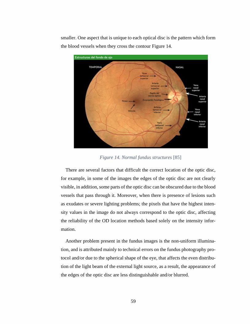
59
smaller. One aspect that is unique to each optical disc is the pattern which form
the blood vessels when they cross the contour Figure 14.
Figure 14. Normal fundus structures [85]
There are several factors that difficult the correct location of the optic disc,
for example, in some of the images the edges of the optic disc are not clearly
visible, in addition, some parts of the optic disc can be obscured due to the blood
vessels that pass through it. Moreover, when there is presence of lesions such
as exudates or severe lighting problems; the pixels that have the highest inten-
sity values in the image do not always correspond to the optic disc, affecting
the reliability of the OD location methods based solely on the intensity infor-
mation.
Another problem present in the fundus images is the non-uniform illumina-
tion, and is attributed mainly to technical errors on the fundus photography pro-
tocol and/or due to the spherical shape of the eye, that affects the even distribu-
tion of the light beam of the external light source, as a result, the appearance of
the edges of the optic disc are less distinguishable and/or blurred.
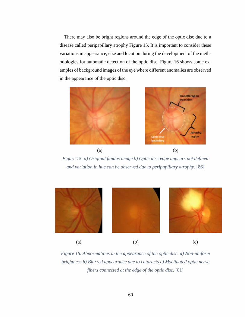
60
There may also be bright regions around the edge of the optic disc due to a
disease called peripapillary atrophy Figure 15. It is important to consider these
variations in appearance, size and location during the development of the meth-
odologies for automatic detection of the optic disc. Figure 16 shows some ex-
amples of background images of the eye where different anomalies are observed
in the appearance of the optic disc.
(a)
(b)
Figure 15. a) Original fundus image b) Optic disc edge appears not defined
and variation in hue can be observed due to peripapillary atrophy. [86]
(a)
(b)
(c)
Figure 16. Abnormalities in the appearance of the optic disc. a) Non-uniform
brightness b) Blurred appearance due to cataracts c) Myelinated optic nerve
fibers connected at the edge of the optic disc. [81]
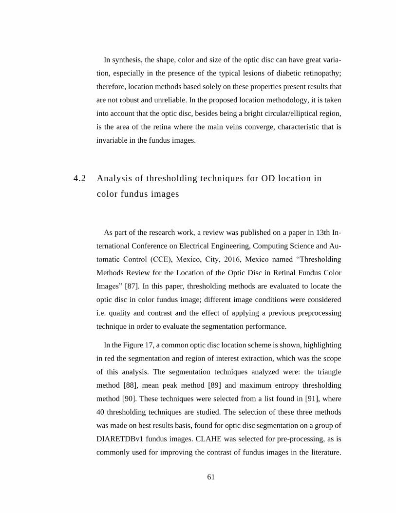
61
In synthesis, the shape, color and size of the optic disc can have great varia-
tion, especially in the presence of the typical lesions of diabetic retinopathy;
therefore, location methods based solely on these properties present results that
are not robust and unreliable. In the proposed location methodology, it is taken
into account that the optic disc, besides being a bright circular/elliptical region,
is the area of the retina where the main veins converge, characteristic that is
invariable in the fundus images.
4.2 Analysis of thresholding techniques for OD location in
color fundus images
As part of the research work, a review was published on a paper in 13th In-
ternational Conference on Electrical Engineering, Computing Science and Au-
tomatic Control (CCE), Mexico, City, 2016, Mexico named “Thresholding
Methods Review for the Location of the Optic Disc in Retinal Fundus Color
Images” [87]. In this paper, thresholding methods are evaluated to locate the
optic disc in color fundus image; different image conditions were considered
i.e. quality and contrast and the effect of applying a previous preprocessing
technique in order to evaluate the segmentation performance.
In the Figure 17, a common optic disc location scheme is shown, highlighting
in red the segmentation and region of interest extraction, which was the scope
of this analysis. The segmentation techniques analyzed were: the triangle
method [88], mean peak method [89] and maximum entropy thresholding
method [90]. These techniques were selected from a list found in [91], where
40 thresholding techniques are studied. The selection of these three methods
was made on best results basis, found for optic disc segmentation on a group of
DIARETDBv1 fundus images. CLAHE was selected for pre-processing, as is
commonly used for improving the contrast of fundus images in the literature.
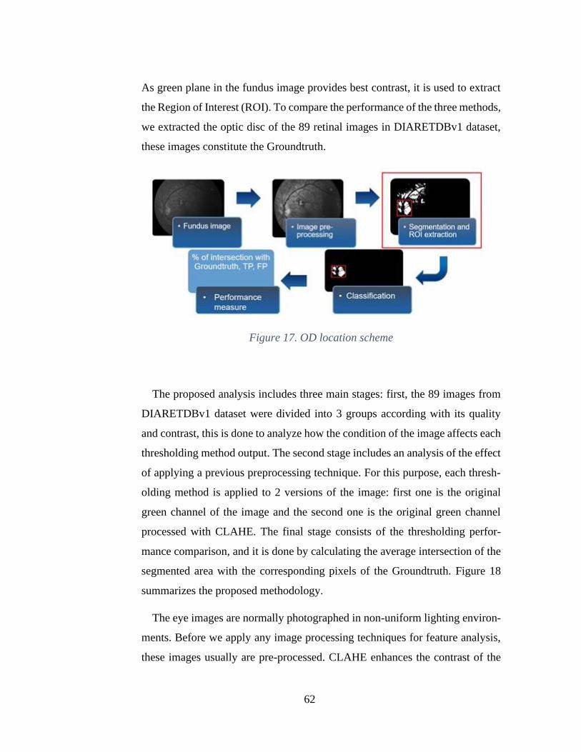
62
As green plane in the fundus image provides best contrast, it is used to extract
the Region of Interest (ROI). To compare the performance of the three methods,
we extracted the optic disc of the 89 retinal images in DIARETDBv1 dataset,
these images constitute the Groundtruth.
Figure 17. OD location scheme
The proposed analysis includes three main stages: first, the 89 images from
DIARETDBv1 dataset were divided into 3 groups according with its quality
and contrast, this is done to analyze how the condition of the image affects each
thresholding method output. The second stage includes an analysis of the effect
of applying a previous preprocessing technique. For this purpose, each thresh-
olding method is applied to 2 versions of the image: first one is the original
green channel of the image and the second one is the original green channel
processed with CLAHE. The final stage consists of the thresholding perfor-
mance comparison, and it is done by calculating the average intersection of the
segmented area with the corresponding pixels of the Groundtruth. Figure 18
summarizes the proposed methodology.
The eye images are normally photographed in non-uniform lighting environ-
ments. Before we apply any image processing techniques for feature analysis,
these images usually are pre-processed. CLAHE enhances the contrast of the
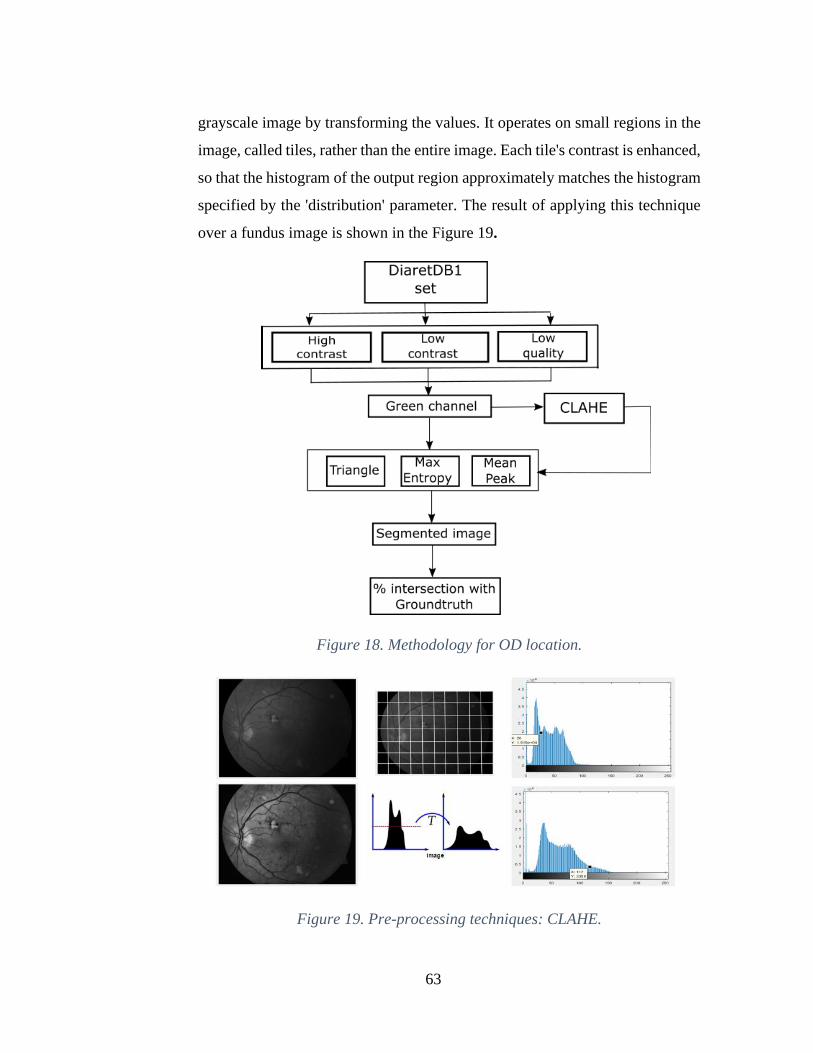
63
grayscale image by transforming the values. It operates on small regions in the
image, called tiles, rather than the entire image. Each tile's contrast is enhanced,
so that the histogram of the output region approximately matches the histogram
specified by the 'distribution' parameter. The result of applying this technique
over a fundus image is shown in the Figure 19.
Figure 18. Methodology for OD location.
Figure 19. Pre-processing techniques: CLAHE.

64
Triangle thresholding technique is particularly effective when the object pix-
els produce a weak peak in the histogram. The result of applying this segmen-
tation method over a fundus image is shown in the Figure 20.
Figure 20. Segmentation methods: Triangle.
Mean Peak thresholding method is based on the form and shape properties of
image histograms. The result of applying this segmentation method over a fun-
dus image is shown in Figure 21.
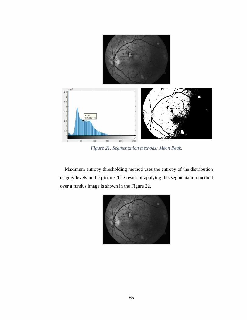
65
Figure 21. Segmentation methods: Mean Peak.
Maximum entropy thresholding method uses the entropy of the distribution
of gray levels in the picture. The result of applying this segmentation method
over a fundus image is shown in the Figure 22.
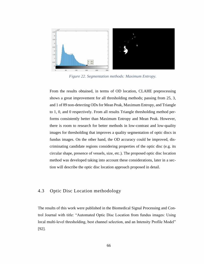
66
Figure 22. Segmentation methods: Maximum Entropy.
From the results obtained, in terms of OD location, CLAHE preprocessing
shows a great improvement for all thresholding methods; passing from 25, 3,
and 1 of 89 non-detecting ODs for Mean Peak, Maximum Entropy, and Triangle
to 1, 0, and 0 respectively. From all results Triangle thresholding method per-
forms consistently better than Maximum Entropy and Mean Peak. However,
there is room to research for better methods in low-contrast and low-quality
images for thresholding that improves a quality segmentation of optic discs in
fundus images. On the other hand, the OD accuracy could be improved, dis-
criminating candidate regions considering properties of the optic disc (e.g. its
circular shape, presence of vessels, size, etc.). The proposed optic disc location
method was developed taking into account these considerations, later in a sec-
tion will describe the optic disc location approach proposed in detail.
4.3 Optic Disc Location methodology
The results of this work were published in the Biomedical Signal Processing and Con-
trol Journal with title: “Automated Optic Disc Location from fundus images: Using
local multi-level thresholding, best channel selection, and an Intensity Profile Model”
[92].
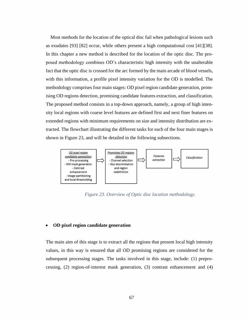
67
Most methods for the location of the optical disc fail when pathological lesions such
as exudates [93] [82] occur, while others present a high computational cost [41][38].
In this chapter a new method is described for the location of the optic disc. The pro-
posed methodology combines OD’s characteristic high intensity with the unalterable
fact that the optic disc is crossed for the arc formed by the main arcade of blood vessels,
with this information, a profile pixel intensity variation for the OD is modelled. The
methodology comprises four main stages: OD pixel region candidate generation, prom-
ising OD regions detection, promising candidate features extraction, and classification.
The proposed method consists in a top-down approach, namely, a group of high inten-
sity local regions with coarse level features are defined first and next finer features on
extended regions with minimum requirements on size and intensity distribution are ex-
tracted. The flowchart illustrating the different tasks for each of the four main stages is
shown in Figure 23, and will be detailed in the following subsections.
Figure 23. Overview of Optic disc location methodology.
• OD pixel region candidate generation
The main aim of this stage is to extract all the regions that present local high intensity
values, in this way is ensured that all OD promising regions are considered for the
subsequent processing stages. The tasks involved in this stage, include: (1) prepro-
cessing, (2) region-of-interest mask generation, (3) contrast enhancement and (4)

68
image partitioning and local thresholding. Table 8. describes the steps of the algorithm
to generate the OD pixel candidate.
As stated before, fundus images quality varies greatly due to many external and internal
factors i.e. fundus camera settings, illumination conditions, spherical geometry of the
eye. To mitigate these undesired effects preprocessing is applied to the fundus image.
To improve softness of the image, a median filter of size 3 × 3 is applied. The filter of
the median is selected because it allows to eliminate artifacts and unwanted structures
in the image without significantly affecting the edges.
Algorithm 1: Candidates generation
1
2
3
4
5
6
7
8
9
10
11
12
13
14
15
input : Original image of dataset (Diaretdb0, Diaretdb1, e-ophtha)
output : Image containing potential OD regions (ImgC)
Preprocess image for noise reduction
Mask out left and right dark region of the image
Redefine initial and final column excluding masked region
Determine OD’s Diameter estimate
Enhance contrast of the green channel
Use one horizontal and three vertical bands for most probable OD location
Begin
for each vertical band
Use 3 threshold bands from maximum to mode pix value
Generate a RGB (ImgC) for the three bands
Red is high threshold band
Green is medium threshold band
Blue is low threshold band
end
End
Table 8. Algorithm to generate the OD pixel candidate.
69
Median filter operates replacing the value of a pixel f(x,y) with the median of all of
the pixels in the neighborhood of that pixel as shown in Equation 1.
𝑓𝑚𝑒𝑑 (𝑥, 𝑦) = 𝑚𝑒𝑑𝑖𝑎𝑛 {𝑓(𝑠, 𝑡)}, 𝑠𝑧 𝜖 𝐼 𝑜𝑑𝑑 𝑎𝑛𝑑 𝑔𝑟𝑒𝑎𝑡𝑒𝑟 𝑡ℎ𝑎𝑛 1,
𝑠 = { 𝑥 −𝑠𝑧 − 1
2 𝑡𝑜 𝑥 +
𝑠𝑧 − 1
2} 𝑎𝑛𝑑 𝑠 ≠ 𝑥,
𝑡 = {𝑦 −𝑠𝑧 − 1
2 𝑡𝑜 𝑦 +
𝑠𝑧 − 1
2} 𝑎𝑛𝑑 𝑡 ≠ 𝑦
Equation 1. Median filter
The ROI rectangle refers to the resulting fundus image where the surrounding dark
zones are excluded. These dark areas are removed to save computing time and to reduce
noise. The semi-circular foreground region is referred as ROI. The mask image is a
binary image where the ROI pixels are set to one and the background pixels to zero.
On Figure 25, the stages for ROI rectangle extraction using the image on Figure 24, are
shown. ROI rectangle for the original image is generated as follows:
(1) The pixels with intensity value below 10 on channels red and green are set to
zero for the purpose to smooth the non-retina zone. (2) A range filter with a 15x15
window is applied. Range filter is used to enhance the borders of the image, as the
highest values correspond to the regions with the highest local variation, the result is
shown in Figure 25(a). The range filter is defined by Equation 2. (3) The 20 percent
highest intensity pixels values are segmented Figure 25(b). (4) A sum of pixels by col-
umn is done, and the rightmost and leftmost peak values with value higher than one
fifth of the image height are selected as ROI first ‘c0’ and last ’c1’ column coordinates.
Rows range are reduced to the 70 percent central band, given that no OD will be at top
or bottom 15 percent. As given in Equation 3.
𝑅𝑎𝑛𝑔𝑒(𝐴(𝑥, 𝑦)) = max[𝐴(𝑥 + 𝑖, 𝑦 + 𝑗)] − min[𝐴(𝑥 + 𝑖, 𝑦 +
𝑗)], 𝑤ℎ𝑒𝑟𝑒 𝑖, 𝑗 𝜖 (−𝑠𝑧−1
2 𝑡𝑜
𝑠𝑧−1
2) , 𝑠𝑧 𝜖 𝐼 𝑜𝑑𝑑 𝑎𝑛𝑑 𝑔𝑟𝑒𝑎𝑡𝑒𝑟 𝑡ℎ𝑎𝑛 1

70
Equation 2. Range filter.
𝑅𝑂𝐼ℎ𝑒𝑖𝑔ℎ𝑡 = [0.15 ∗ ℎ𝑒𝑖𝑔ℎ𝑡 𝑡𝑜 0.85 ∗ ℎ𝑒𝑖𝑔ℎ𝑡, 𝑐0 𝑡𝑜 𝑐1],
𝑅𝑂𝐼𝑤𝑖𝑑𝑡ℎ = 𝑐0 − 𝑐1 + 1
Equation 3. ROI width and height definition.
OD diameter approximate value, is defined as 𝐷𝑖𝑎𝑚 = ⌊𝑅𝑂𝐼𝑤𝑖𝑑𝑡ℎ
6⌋.
Figure 24. Original fundus image.
(a)
(b)
(c)
Figure 25. (a) Result of applying a range filter with a 15x15 window. (b) Re-
sult of applying a threshold of the highest 20 percent of image (a). (c) Re-
gion-of-interest (ROI) rectangle (red).
From the previous analysis, CLAHE showed promising results for improving the
contrast and the OD thresholding results. Other conventional methods based on the
global histogram of the image such as contrast stretching and histogram equalization,
tend to result in loss of information in the brightest areas as well as in the dark areas of

71
the background image. CLAHE operates in small regions of the image, improving the
contrast by local equalization of the histogram, whereby small regions of interest are
highlighted throughout the image. To enhance contrast of the fundus image, CLAHE
is applied to the green channel of the ROI rectangle.
As mentioned earlier, non-uniform illumination induces undesired local intensity vari-
ations, hence the application of a global high intensity threshold value to locate the OD
region is not reliable. To extract more meaningful information from the fundus image,
a partition into windows or sub-images for the extraction of local OD candidate regions
is applied. The image division is done accordingly to the previously estimated OD di-
ameter: one horizontal band and three vertical bands are defined based on OD’s diam-
eter. For each of the three bands, a threshold based on the maximum and the mode
intensity value is calculated. Using the green channel, the sub-divisions and local
threshold values are defined as:
Horizontal band: 𝒘𝒊𝒏𝑹 = [1.25 ∗
𝐷𝑖𝑎𝑚 𝑡𝑜 𝑖𝑚𝑎𝑔𝑒𝐻𝑒𝑖𝑔ℎ𝑡 − 1.75 ∗ 𝐷𝑖𝑎𝑚]
Vertical bands: 𝒘𝒊𝒏𝑪 = { [𝑐0 𝑡𝑜 1.75 ∗ 𝐷𝑖𝑎𝑚], (1.75 ∗
𝐷𝑖𝑎𝑚 𝑡𝑜 3.75 ∗ 𝐷𝑖𝑎𝑚], (3.75 ∗ 𝐷𝑖𝑎𝑚 𝑡𝑜 𝑐1 ]}
𝒅𝒆𝒍𝒕𝒂 =𝑤𝑖𝑛𝑑𝑜𝑤 max 𝑣𝑎𝑙𝑢𝑒 − 𝑤𝑖𝑛𝑑𝑜𝑤 𝑚𝑜𝑑𝑒 𝑣𝑎𝑙𝑢𝑒
4.75
𝒕𝒉𝒓𝒆𝒔𝒉𝒐𝒍𝒅 = 𝑤𝑖𝑛𝑑𝑜𝑤 max 𝑣𝑎𝑙𝑢𝑒 − 𝑑𝑒𝑙𝑡𝑎
For each of the three defined sub-regions, the pixels with intensity values higher than
their local threshold, are considered as possible OD regions, and together conform the
image containing the OD candidates (ImgODcand). On Figure 26, an illustration of fun-
dus image partitioning along with the result of applying their local thresholding is
shown.

72
(a)
(b)
Figure 26. (a) Original fundus image (b) Image partitioning and local thresh-
olding. ImgODcand is the set of all red sub-regions.
• Promising OD regions detection
Once all the relevant local high intensity regions are extracted, more detailed features
select most promising ones. The approach consists in going from a group of regions
with coarse level features to finer features on extended regions with minimum require-
ments on size and intensity distribution. The steps to select regions with better charac-
teristics to contain an OD, include the channel selection, which is done by selecting the
one with better contrast between red and green channels. For contrast evaluation, the
image is partitioned, a median filter of size 7 × 7 is applied to both channels and an
index based on the difference between the maximum intensity and the mode value of
each subregion is calculated by Equation 4.
𝑖𝑐 =𝑚𝑎𝑥𝑖𝑚𝑢𝑚 𝑖𝑛𝑡𝑒𝑛𝑠𝑖𝑡𝑦 𝑣𝑎𝑙𝑢𝑒 − 𝑚𝑜𝑑𝑒 𝑣𝑎𝑙𝑢𝑒
𝑚𝑜𝑑𝑒 𝑣𝑎𝑙𝑢𝑒
Equation 4. Index for contrast evaluation
73
As high contrast images show a wide distribution of gray levels in their histograms,
and as mode intensity value is an approximation of the background intensity value (ret-
inal tissue), the higher ic index indicates the channel which has a major level of differ-
entiations between the background and the bright structures of the retina, including the
OD. The channel with better contrast between green and red is selected for posterior
processing.
As the images from the datasets present different resolutions, all the size constraints
are defined with respect to the Diam value, in this way the proposed methodology is
independent from image resolution. For the size discrimination of the region candidates
from ImgODcand, a minimum of (1/20)*Diam and a maximum of Diam for height and
width is established. Then, to analyze the local distribution of each remaining region
candidate, is necessary to center around the pixels with higher intensity and extend the
size to match with the actual OD size. The center is calculated using the ’WeightedCen-
troid’ concept, which considers pixel intensities in the image region as weights in the
centroid calculation, intensities used are defined by the yellowish proportion of pixels
in the region. Then, the region is extended around the centroid coordinates by half of
Diam. Next, a threshold value is calculated for each candidate:
𝑑𝑖𝑓𝑓 = (𝑚𝑎𝑥𝑖𝑚𝑢𝑚 𝑣𝑎𝑙𝑢𝑒 − 𝑚𝑜𝑑𝑒 𝑣𝑎𝑙𝑢𝑒)
𝑑𝑒𝑙𝑡𝑎 = {
𝑑𝑖𝑓𝑓
4.75, 𝑖𝑓 𝑑𝑖𝑓𝑓 > 30
6 , 𝑖𝑓 𝑑𝑖𝑓𝑓 ≤ 30
𝑇ℎ𝑟𝑒𝑠ℎ𝑜𝑙𝑑𝑒 = 𝑚𝑎𝑥𝑖𝑚𝑢𝑚 𝑣𝑎𝑙𝑢𝑒 − 3 ∗ 𝑑𝑒𝑙𝑡𝑎
Thresholde aims to segment a high intensity section of the histogram, as generally
optic disc cup shows higher intensity than OD. The resulting regions again are filtered
by size: minimum and width and height of Diam/10 and Diam/8, respectively.
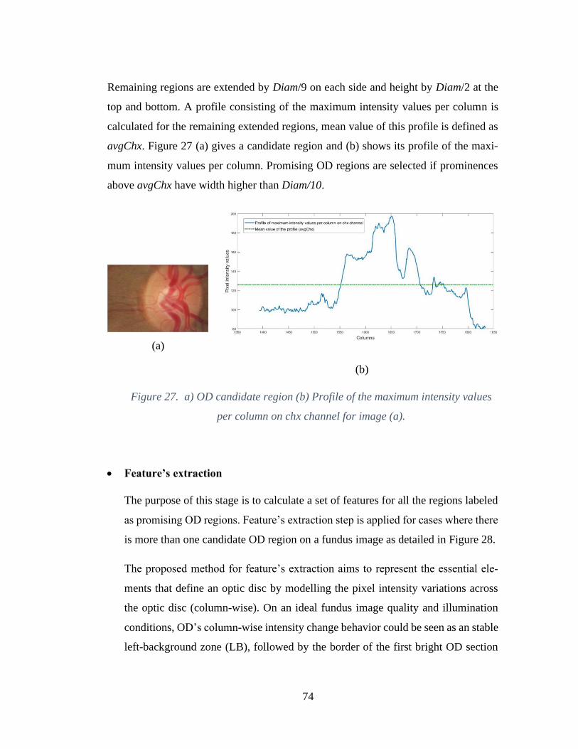
74
Remaining regions are extended by Diam/9 on each side and height by Diam/2 at the
top and bottom. A profile consisting of the maximum intensity values per column is
calculated for the remaining extended regions, mean value of this profile is defined as
avgChx. Figure 27 (a) gives a candidate region and (b) shows its profile of the maxi-
mum intensity values per column. Promising OD regions are selected if prominences
above avgChx have width higher than Diam/10.
(a)
(b)
Figure 27. a) OD candidate region (b) Profile of the maximum intensity values
per column on chx channel for image (a).
• Feature’s extraction
The purpose of this stage is to calculate a set of features for all the regions labeled
as promising OD regions. Feature’s extraction step is applied for cases where there
is more than one candidate OD region on a fundus image as detailed in Figure 28.
The proposed method for feature’s extraction aims to represent the essential ele-
ments that define an optic disc by modelling the pixel intensity variations across
the optic disc (column-wise). On an ideal fundus image quality and illumination
conditions, OD’s column-wise intensity change behavior could be seen as an stable
left-background zone (LB), followed by the border of the first bright OD section
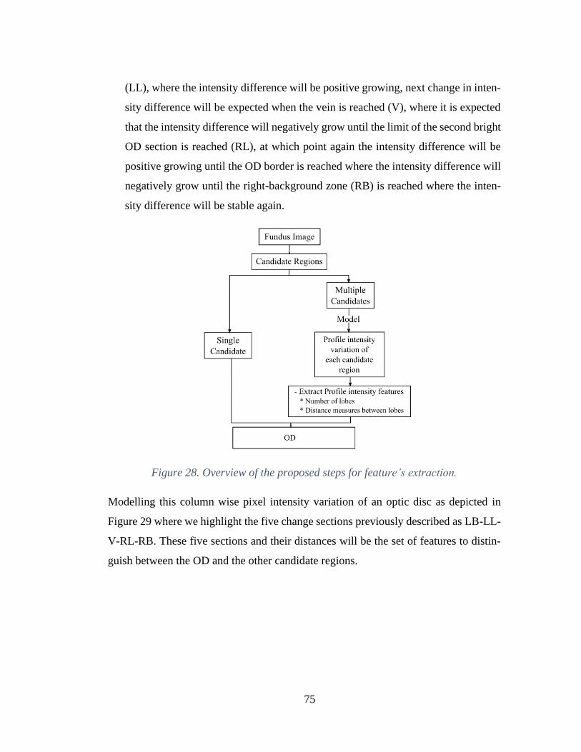
75
(LL), where the intensity difference will be positive growing, next change in inten-
sity difference will be expected when the vein is reached (V), where it is expected
that the intensity difference will negatively grow until the limit of the second bright
OD section is reached (RL), at which point again the intensity difference will be
positive growing until the OD border is reached where the intensity difference will
negatively grow until the right-background zone (RB) is reached where the inten-
sity difference will be stable again.
Figure 28. Overview of the proposed steps for feature’s extraction.
Modelling this column wise pixel intensity variation of an optic disc as depicted in
Figure 29 where we highlight the five change sections previously described as LB-LL-
V-RL-RB. These five sections and their distances will be the set of features to distin-
guish between the OD and the other candidate regions.
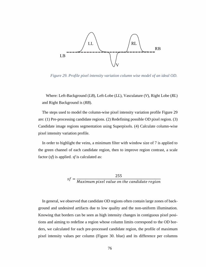
76
Figure 29. Profile pixel intensity variation column wise model of an ideal OD.
Where: Left-Background (LB), Left-Lobe (LL), Vasculature (V), Right Lobe (RL)
and Right Background is (RB).
The steps used to model the column-wise pixel intensity variation profile Figure 29
are: (1) Pre-processing candidate regions. (2) Redefining possible OD pixel region. (3)
Candidate image regions segmentation using Superpixels. (4) Calculate column-wise
pixel intensity variation profile.
In order to highlight the veins, a minimum filter with window size of 7 is applied to
the green channel of each candidate region, then to improve region contrast, a scale
factor (sf) is applied. sf is calculated as:
𝑠𝑓 =255
𝑀𝑎𝑥𝑖𝑚𝑢𝑚 𝑝𝑖𝑥𝑒𝑙 𝑣𝑎𝑙𝑢𝑒 𝑜𝑛 𝑡ℎ𝑒 𝑐𝑎𝑛𝑑𝑖𝑑𝑎𝑡𝑒 𝑟𝑒𝑔𝑖𝑜𝑛
In general, we observed that candidate OD regions often contain large zones of back-
ground and undesired artifacts due to low quality and the non-uniform illumination.
Knowing that borders can be seen as high intensity changes in contiguous pixel posi-
tions and aiming to redefine a region whose column limits correspond to the OD bor-
ders, we calculated for each pre-processed candidate region, the profile of maximum
pixel intensity values per column (Figure 30. blue) and its difference per columns
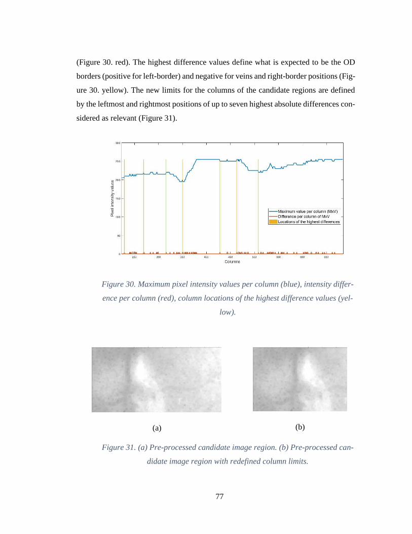
77
(Figure 30. red). The highest difference values define what is expected to be the OD
borders (positive for left-border) and negative for veins and right-border positions (Fig-
ure 30. yellow). The new limits for the columns of the candidate regions are defined
by the leftmost and rightmost positions of up to seven highest absolute differences con-
sidered as relevant (Figure 31).
Figure 30. Maximum pixel intensity values per column (blue), intensity differ-
ence per column (red), column locations of the highest difference values (yel-
low).
(a)
(b)
Figure 31. (a) Pre-processed candidate image region. (b) Pre-processed can-
didate image region with redefined column limits.
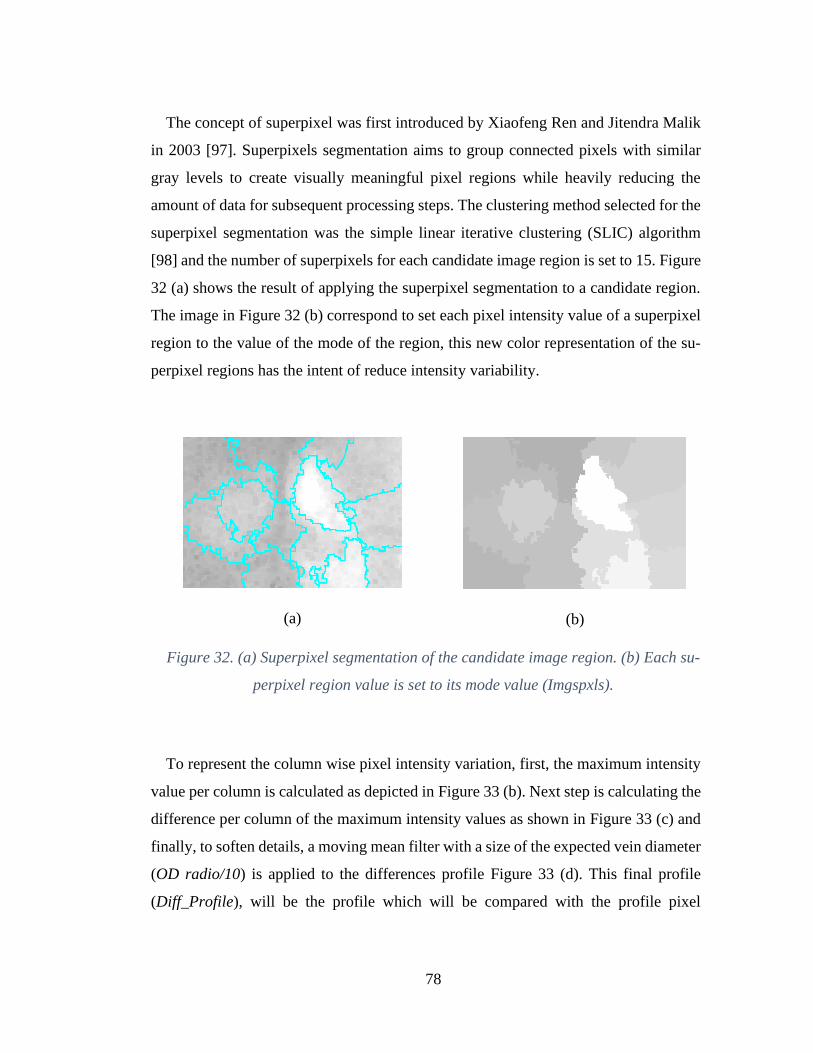
78
The concept of superpixel was first introduced by Xiaofeng Ren and Jitendra Malik
in 2003 [97]. Superpixels segmentation aims to group connected pixels with similar
gray levels to create visually meaningful pixel regions while heavily reducing the
amount of data for subsequent processing steps. The clustering method selected for the
superpixel segmentation was the simple linear iterative clustering (SLIC) algorithm
[98] and the number of superpixels for each candidate image region is set to 15. Figure
32 (a) shows the result of applying the superpixel segmentation to a candidate region.
The image in Figure 32 (b) correspond to set each pixel intensity value of a superpixel
region to the value of the mode of the region, this new color representation of the su-
perpixel regions has the intent of reduce intensity variability.
(a)
(b)
Figure 32. (a) Superpixel segmentation of the candidate image region. (b) Each su-
perpixel region value is set to its mode value (Imgspxls).
To represent the column wise pixel intensity variation, first, the maximum intensity
value per column is calculated as depicted in Figure 33 (b). Next step is calculating the
difference per column of the maximum intensity values as shown in Figure 33 (c) and
finally, to soften details, a moving mean filter with a size of the expected vein diameter
(OD radio/10) is applied to the differences profile Figure 33 (d). This final profile
(Diff_Profile), will be the profile which will be compared with the profile pixel
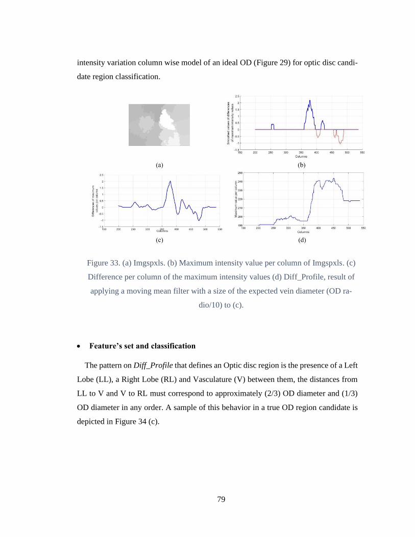
79
intensity variation column wise model of an ideal OD (Figure 29) for optic disc candi-
date region classification.
Figure 33. (a) Imgspxls. (b) Maximum intensity value per column of Imgspxls. (c)
Difference per column of the maximum intensity values (d) Diff_Profile, result of
applying a moving mean filter with a size of the expected vein diameter (OD ra-
dio/10) to (c).
• Feature’s set and classification
The pattern on Diff_Profile that defines an Optic disc region is the presence of a Left
Lobe (LL), a Right Lobe (RL) and Vasculature (V) between them, the distances from
LL to V and V to RL must correspond to approximately (2/3) OD diameter and (1/3)
OD diameter in any order. A sample of this behavior in a true OD region candidate is
depicted in Figure 34 (c).
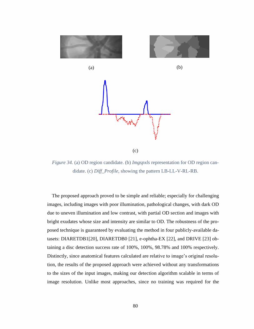
80
(a)
(b)
(c)
Figure 34. (a) OD region candidate. (b) Imgspxls representation for OD region can-
didate. (c) Diff_Profile, showing the pattern LB-LL-V-RL-RB.
The proposed approach proved to be simple and reliable; especially for challenging
images, including images with poor illumination, pathological changes, with dark OD
due to uneven illumination and low contrast, with partial OD section and images with
bright exudates whose size and intensity are similar to OD. The robustness of the pro-
posed technique is guaranteed by evaluating the method in four publicly-available da-
tasets: DIARETDB1[20], DIARETDB0 [21], e-ophtha-EX [22], and DRIVE [23] ob-
taining a disc detection success rate of 100%, 100%, 98.78% and 100% respectively.
Distinctly, since anatomical features calculated are relative to image’s original resolu-
tion, the results of the proposed approach were achieved without any transformations
to the sizes of the input images, making our detection algorithm scalable in terms of
image resolution. Unlike most approaches, since no training was required for the

81
classification stage, no additional datasets are needed for this task and the results are
calculated using all images of the datasets.
4.4 Detection of the fovea, macula and exudates for the pre-di-
agnosis of Diabetic Macular Edema (DME)
Diabetic Macular Edema (DME), an important complication of DR, occurs when the
leakage of blood vessels causes accumulation of fluid in the macula region. In clinical
practice, ophthalmologists diagnose DME based on the presence of exudates in the
macular neighborhood. The macula corresponds to the central area of the retina, re-
sponsible for the most accurate and color vision due its high density of photoreceptors.
Since the pigmented epithelial cells in the macula are taller and contain more pigment
compared to cells elsewhere in the retina, the fovea region appears to be the darkest
region of the retina. This region is also devoid of retinal blood vessels. The fovea is the
shallow depression located at the center of the macular region. Fovea has an oval shape
and a diameter equal to 1.5mm being nearly equal to the diameter of the optic disc. In
addition, OD location can be used for fovea center estimation since both structures are
separated approximately at a constant distance of 2.5 OD diameter. The severity of
DME is evaluated by the presence of exudates in a determined region around fovea. It
is called Clinically Significant Macular Edema (CSME), if exudates presence is con-
firmed in the circle of 1 OD diameter around fovea and Non-Clinically Significant
Macular Edema, when there is presence of exudates outside the region defined around
1 OD diameter around fovea. Hence, automatic detection of fovea is essential in the
development of computer-aided diagnosis (CAD) system for DR and DME.
The challenges for the accurate localization of the fovea includes the presence of hem-
orrhages which could be similar in shape, size and intensity. Moreover, the localization
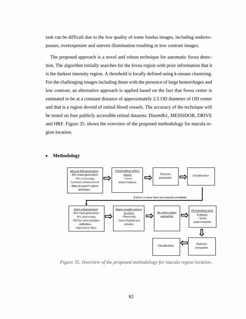
82
task can be difficult due to the low quality of some fundus images, including underex-
posure, overexposure and uneven illumination resulting in low contrast images.
The proposed approach is a novel and robust technique for automatic fovea detec-
tion. The algorithm initially searches for the fovea region with prior information that it
is the darkest intensity region. A threshold is locally defined using k-means clustering.
For the challenging images including those with the presence of large hemorrhages and
low contrast, an alternative approach is applied based on the fact that fovea center is
estimated to be at a constant distance of approximately 2.5 OD diameter of OD center
and that is a region devoid of retinal blood vessels. The accuracy of the technique will
be tested on four publicly accessible retinal datasets: Diaretdb1, MESSIDOR, DRIVE
and HRF. Figure 35. shows the overview of the proposed methodology for macula re-
gion location.
• Methodology
Figure 35. Overview of the proposed methodology for macula region location.
Features
Extraction
Classification
If there is more than one macula candidate

83
• Macula ROI location
The purpose of this stage is to determine the region of interest corresponding to macula.
First, applying the same procedure as for optic disc location, the dark zones surround-
ing fundus image are excluded from further processing, and the approximation of the
diameter Diam is calculated.
In general, macula is located in the central region of the fundus images. Then, to reduce
the macula search region, image height is redefined by Equation 5 and image width as
Equation 6.
𝑤𝑖𝑛𝑅 = ([𝑟0 (1.25 ∗ 𝐷𝑖𝑎𝑚) (𝑟1 − (1.25 ∗ 𝐷𝑖𝑎𝑚))])
Equation 5. Image height definition
𝑤𝑖𝑛𝐶 = ([𝑐0 (𝑐0 + 1.25 ∗ 𝐷𝑖𝑎𝑚) (𝑐0 + (4.5 ∗ 𝐷𝑖𝑎𝑚)) 𝑐1])
Equation 6. Image width definition
Pre-processing includes applying a minimum filter with size of 5x5, to enhance the
darker structures of the fundus image. CLAHE is used for contrast improvement and a
moving mean filter of size 5x5 for noise reduction. Figure 37. illustrates the macula
ROI generation steps.
Figure 36. Original fundus image.
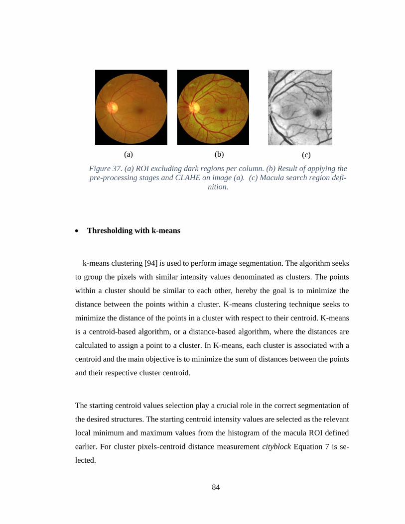
84
(a)
(b)
(c)
Figure 37. (a) ROI excluding dark regions per column. (b) Result of applying the
pre-processing stages and CLAHE on image (a). (c) Macula search region defi-
nition.
• Thresholding with k-means
k-means clustering [94] is used to perform image segmentation. The algorithm seeks
to group the pixels with similar intensity values denominated as clusters. The points
within a cluster should be similar to each other, hereby the goal is to minimize the
distance between the points within a cluster. K-means clustering technique seeks to
minimize the distance of the points in a cluster with respect to their centroid. K-means
is a centroid-based algorithm, or a distance-based algorithm, where the distances are
calculated to assign a point to a cluster. In K-means, each cluster is associated with a
centroid and the main objective is to minimize the sum of distances between the points
and their respective cluster centroid.
The starting centroid values selection play a crucial role in the correct segmentation of
the desired structures. The starting centroid intensity values are selected as the relevant
local minimum and maximum values from the histogram of the macula ROI defined
earlier. For cluster pixels-centroid distance measurement cityblock Equation 7 is se-
lected.
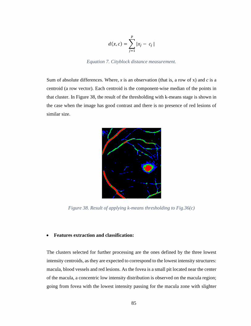
85
𝑑(𝑥, 𝑐) = ∑ |𝑥𝑗 − 𝑐𝑗
𝑝
𝑗=1
|
Equation 7. Cityblock distance measurement.
Sum of absolute differences. Where, x is an observation (that is, a row of x) and c is a
centroid (a row vector). Each centroid is the component-wise median of the points in
that cluster. In Figure 38, the result of the thresholding with k-means stage is shown in
the case when the image has good contrast and there is no presence of red lesions of
similar size.
Figure 38. Result of applying k-means thresholding to Fig.36(c)
• Features extraction and classification:
The clusters selected for further processing are the ones defined by the three lowest
intensity centroids, as they are expected to correspond to the lowest intensity structures:
macula, blood vessels and red lesions. As the fovea is a small pit located near the center
of the macula, a concentric low intensity distribution is observed on the macula region;
going from fovea with the lowest intensity passing for the macula zone with slighter
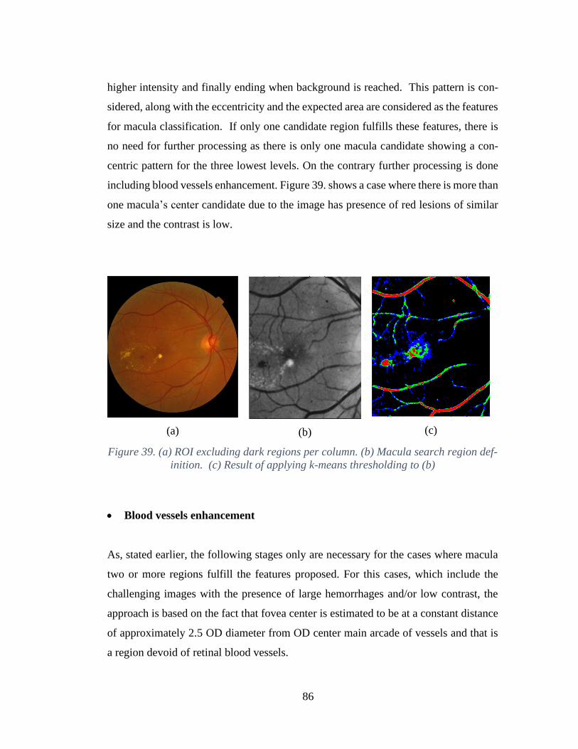
86
higher intensity and finally ending when background is reached. This pattern is con-
sidered, along with the eccentricity and the expected area are considered as the features
for macula classification. If only one candidate region fulfills these features, there is
no need for further processing as there is only one macula candidate showing a con-
centric pattern for the three lowest levels. On the contrary further processing is done
including blood vessels enhancement. Figure 39. shows a case where there is more than
one macula’s center candidate due to the image has presence of red lesions of similar
size and the contrast is low.
(a)
(b)
(c)
Figure 39. (a) ROI excluding dark regions per column. (b) Macula search region def-
inition. (c) Result of applying k-means thresholding to (b)
• Blood vessels enhancement
As, stated earlier, the following stages only are necessary for the cases where macula
two or more regions fulfill the features proposed. For this cases, which include the
challenging images with the presence of large hemorrhages and/or low contrast, the
approach is based on the fact that fovea center is estimated to be at a constant distance
of approximately 2.5 OD diameter from OD center main arcade of vessels and that is
a region devoid of retinal blood vessels.
87
The pre-processing and ROI mask stages are the same from the macula ROI generation
stage, as from ROI for veins location definition, width is defined by winR and height
by winC:
𝑤𝑖𝑛𝑅 = ([1 + (𝑟 ∗ 0.15) 𝑟 − (𝑟 ∗ 0.85)])
Equation 8. Image height definition
𝑤𝑖𝑛𝐶 = ([𝑐0 + 0.5 ∗ 𝐷𝑖𝑎𝑚 (𝑐1 − (0.5 ∗ 𝐷𝑖𝑎𝑚)) ])
Equation 9. Image width definition
Then, next step consists in finding the main arcade vessels, for this purpose vessel en-
hancement is applied. Vessels are enhanced using the fibermetric filter [95], this filter
was specifically designed by the authors for blood vessel enhancement on magnetic
resonance angiography images (MRA) and digital subtraction angiography images
(DSA).
This technique seeks for tubular regions using the local second order ellipsoid. The
result of applying this filtering with a window size of Diam/9 to the image of Figure
40 (a) is shown in Figure 40 (b).
• Major arcade column location and no vessels region extraction
Once, vessels are enhanced, next step consists in applying thresholding to extract the
major arcade of vessels. The fibermetric filter response is higher in the dark objects
whose size approximates to the window size, for this reason the threshold is set to the
25% highest intensity pixels, the result of applying this threshold is shown in Figure
40 (c). Next, a vector consisting of the sum column of pixels with width Diam/9 is
calculated, the major arcade location is found as the maximum peak value location
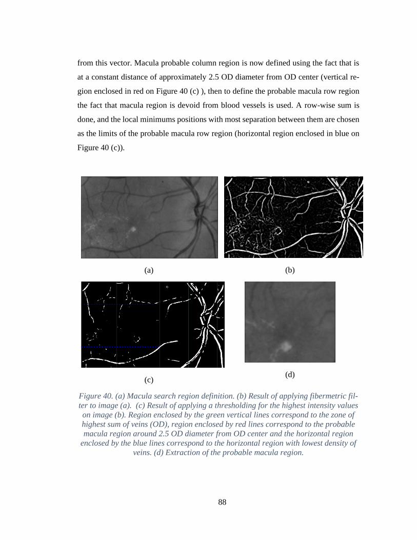
88
from this vector. Macula probable column region is now defined using the fact that is
at a constant distance of approximately 2.5 OD diameter from OD center (vertical re-
gion enclosed in red on Figure 40 (c) ), then to define the probable macula row region
the fact that macula region is devoid from blood vessels is used. A row-wise sum is
done, and the local minimums positions with most separation between them are chosen
as the limits of the probable macula row region (horizontal region enclosed in blue on
Figure 40 (c)).
(a)
(b)
(c)
(d)
Figure 40. (a) Macula search region definition. (b) Result of applying fibermetric fil-
ter to image (a). (c) Result of applying a thresholding for the highest intensity values
on image (b). Region enclosed by the green vertical lines correspond to the zone of
highest sum of veins (OD), region enclosed by red lines correspond to the probable
macula region around 2.5 OD diameter from OD center and the horizontal region
enclosed by the blue lines correspond to the horizontal region with lowest density of
veins. (d) Extraction of the probable macula region.
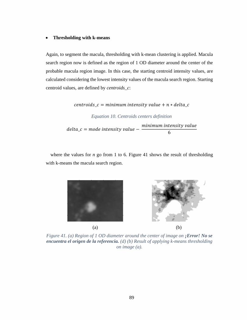
89
• Thresholding with k-means
Again, to segment the macula, thresholding with k-mean clustering is applied. Macula
search region now is defined as the region of 1 OD diameter around the center of the
probable macula region image. In this case, the starting centroid intensity values, are
calculated considering the lowest intensity values of the macula search region. Starting
centroid values, are defined by centroids_c:
𝑐𝑒𝑛𝑡𝑟𝑜𝑖𝑑𝑠_𝑐 = 𝑚𝑖𝑛𝑖𝑚𝑢𝑚 𝑖𝑛𝑡𝑒𝑛𝑠𝑖𝑡𝑦 𝑣𝑎𝑙𝑢𝑒 + 𝑛 ∗ 𝑑𝑒𝑙𝑡𝑎_𝑐
Equation 10. Centroids centers definition
𝑑𝑒𝑙𝑡𝑎_𝑐 = 𝑚𝑜𝑑𝑒 𝑖𝑛𝑡𝑒𝑛𝑠𝑖𝑡𝑦 𝑣𝑎𝑙𝑢𝑒 − 𝑚𝑖𝑛𝑖𝑚𝑢𝑚 𝑖𝑛𝑡𝑒𝑛𝑠𝑖𝑡𝑦 𝑣𝑎𝑙𝑢𝑒
6
where the values for n go from 1 to 6. Figure 41 shows the result of thresholding
with k-means the macula search region.
(a)
(b)
Figure 41. (a) Region of 1 OD diameter around the center of image on ¡Error! No se
encuentra el origen de la referencia. (d) (b) Result of applying k-means thresholding
on image (a).
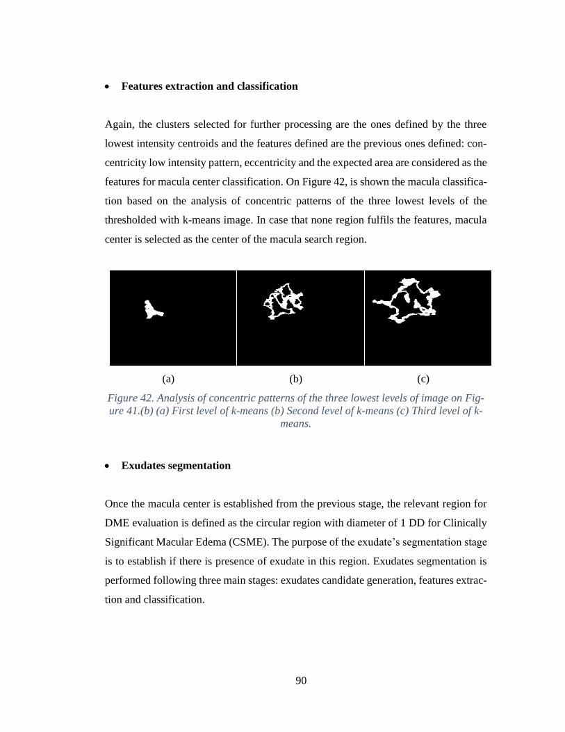
90
• Features extraction and classification
Again, the clusters selected for further processing are the ones defined by the three
lowest intensity centroids and the features defined are the previous ones defined: con-
centricity low intensity pattern, eccentricity and the expected area are considered as the
features for macula center classification. On Figure 42, is shown the macula classifica-
tion based on the analysis of concentric patterns of the three lowest levels of the
thresholded with k-means image. In case that none region fulfils the features, macula
center is selected as the center of the macula search region.
(a)
(b)
(c)
Figure 42. Analysis of concentric patterns of the three lowest levels of image on Fig-
ure 41.(b) (a) First level of k-means (b) Second level of k-means (c) Third level of k-
means.
• Exudates segmentation
Once the macula center is established from the previous stage, the relevant region for
DME evaluation is defined as the circular region with diameter of 1 DD for Clinically
Significant Macular Edema (CSME). The purpose of the exudate’s segmentation stage
is to establish if there is presence of exudate in this region. Exudates segmentation is
performed following three main stages: exudates candidate generation, features extrac-
tion and classification.
91
• Exudates region candidate generation
The purpose of this stage is to generate all the bright regions that potentially could be
classified as exudates. First, the circular region with diameter of 1 DD around the mac-
ula center calculated is extracted for further processing. Preprocessing with median
filtering with size 3x3 is applied to the green and red channel to reduce noise. Next, a
channel which we named GR is calculated dividing the green channel by the red chan-
nel. GR channel creation aims to represent the yellow tonalities found in the image, as
it is known that exudates present this color characteristic in fundus images. As the per-
ception of contrast varies according with the range of grays levels present in the image,
when the majority of the pixels are concentrated on the low intensity gray values, the
brighter regions are less distinguishable. For this reason, in the cases where the yellow
tonalities found are of low value, a sharpening filter [96] is applied in order to accen-
tuate the borders. The index pM is proposed to evaluate if the majority of the yellow
tonalities found are of low value. pM is calculated as the division of the mode of the
green channel by the mode of the green channel. Sharpening filter is applied only if pM
value is lower than 0.4.
From the observation of the patterns of exudates lesions, we determined that exu-
dates intensity variation present a gradual shift in concentric form, going from high
intensity values at its center to lower values as background is reached. Aiming to rep-
resent this pattern, a contour map of the image is calculated. The contour map [97] is
represented by isolines, a series of curves along where the function has a constant value,
so that the curve joins points of equal value. More generally, a contour line for a func-
tion of two variables is a curve connecting points where the function has the same or
similar value. The number of contours for the contour map representation is set to five,
as the top three are expected to represent the brighter structures, the lower the dark
objects, including the vessels and the second contour aims to represent the background.
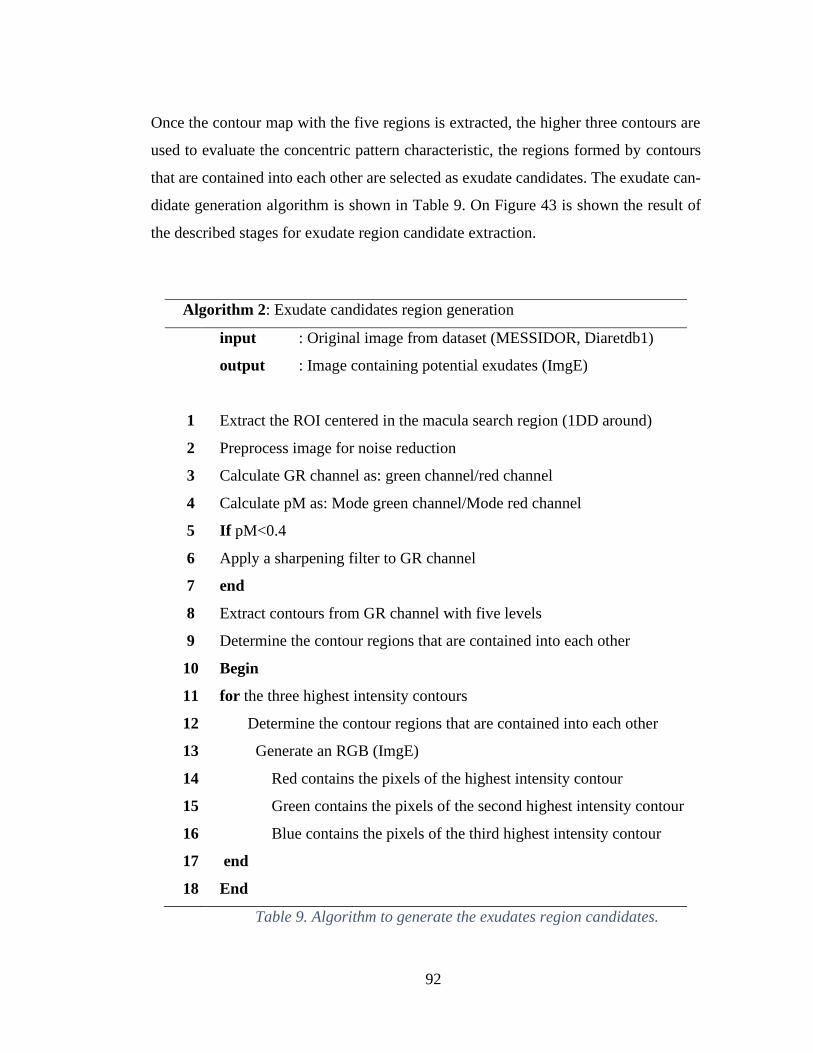
92
Once the contour map with the five regions is extracted, the higher three contours are
used to evaluate the concentric pattern characteristic, the regions formed by contours
that are contained into each other are selected as exudate candidates. The exudate can-
didate generation algorithm is shown in Table 9. On Figure 43 is shown the result of
the described stages for exudate region candidate extraction.
Algorithm 2: Exudate candidates region generation
1
2
3
4
5
6
7
8
9
10
11
12
13
14
15
16
17
18
input : Original image from dataset (MESSIDOR, Diaretdb1)
output : Image containing potential exudates (ImgE)
Extract the ROI centered in the macula search region (1DD around)
Preprocess image for noise reduction
Calculate GR channel as: green channel/red channel
Calculate pM as: Mode green channel/Mode red channel
If pM<0.4
Apply a sharpening filter to GR channel
end
Extract contours from GR channel with five levels
Determine the contour regions that are contained into each other
Begin
for the three highest intensity contours
Determine the contour regions that are contained into each other
Generate an RGB (ImgE)
Red contains the pixels of the highest intensity contour
Green contains the pixels of the second highest intensity contour
Blue contains the pixels of the third highest intensity contour
end
End
Table 9. Algorithm to generate the exudates region candidates.
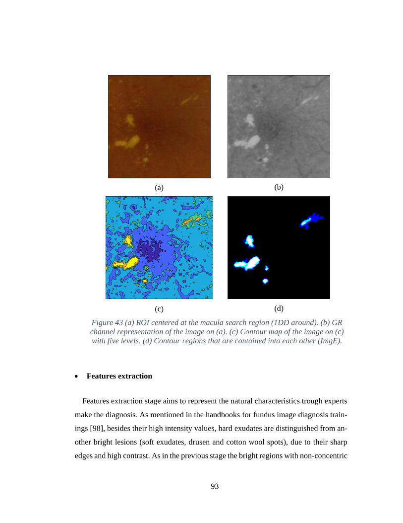
93
(a)
(b)
(c)
(d)
Figure 43 (a) ROI centered at the macula search region (1DD around). (b) GR
channel representation of the image on (a). (c) Contour map of the image on (c)
with five levels. (d) Contour regions that are contained into each other (ImgE).
• Features extraction
Features extraction stage aims to represent the natural characteristics trough experts
make the diagnosis. As mentioned in the handbooks for fundus image diagnosis train-
ings [98], besides their high intensity values, hard exudates are distinguished from an-
other bright lesions (soft exudates, drusen and cotton wool spots), due to their sharp
edges and high contrast. As in the previous stage the bright regions with non-concentric

94
intensity variations were filtered, the following measurements are proposed to calculate
the contrast and the edge sharpness:
- Maximum green intensity value of the pixels conforming the candidate region.
- Mean green intensity value of the pixels conforming the candidate region.
- The number of different gray levels found in the region in the green channel.
- Maximum border intensity value: calculated extending the candidate region and
applying the range filter. The region is extended in order to include background
information.
These four features are extracted for each candidate region per image, and are ar-
ranged in a vector named the feature vector. Table 10 summarizes the algorithm for
exudates features extraction.
Algorithm 3: Exudate features extraction
1
2
3
4
5
1. 6
6
2. 8
7
input : Image containing potential exudates (ImgE)
output : A vector containing the set of features to classify
the exudate regions (Feature_Vector)
Begin
for each candidate region of ImgE extract
Maximum green intensity value of the region (mgI)
Mean green intensity value of the pixels of the region (avgI)
(nLv) as the number of different gray levels found in the region in the
green channel
Maximum border intensity value: calculated extending the
candidate region and applying the range filter (mbI)
Feature_Vector=[mgI; avgI; nLv; mbI]
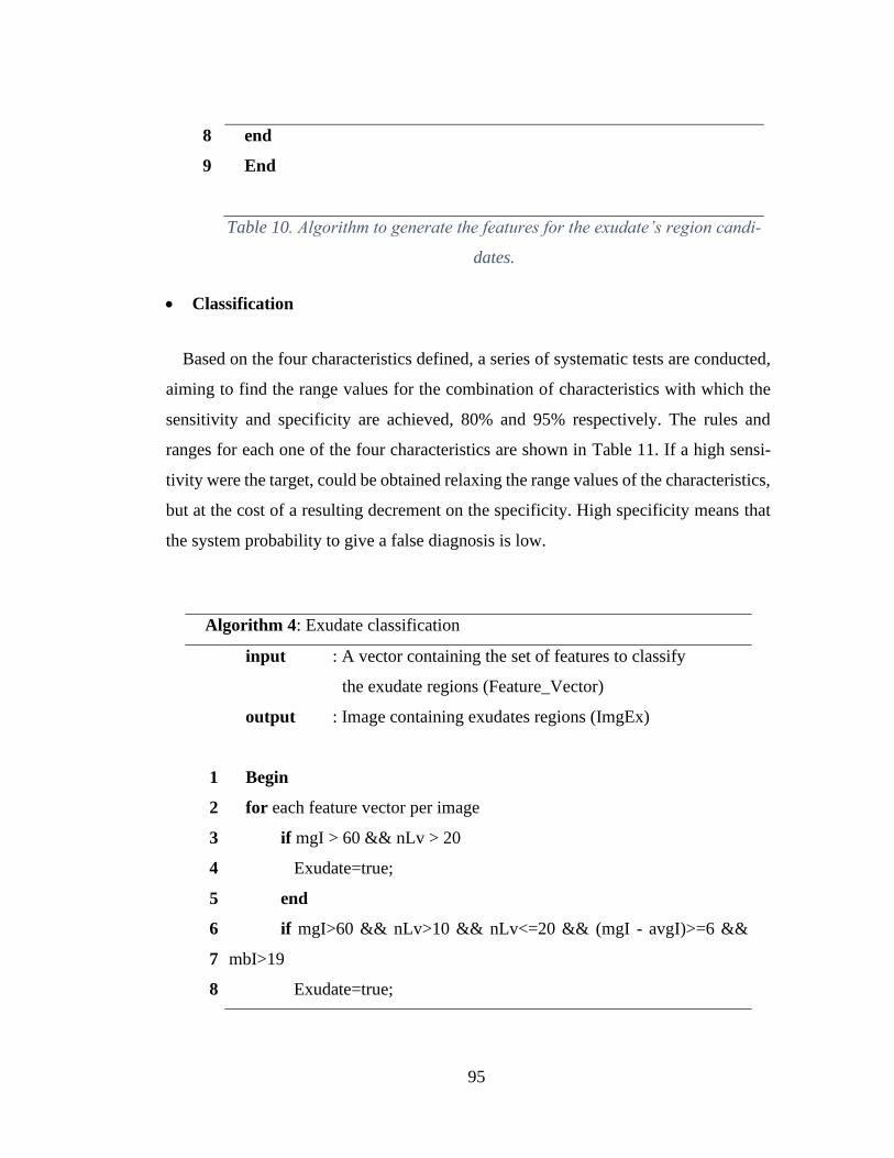
95
8
9
end
End
Table 10. Algorithm to generate the features for the exudate’s region candi-
dates.
• Classification
Based on the four characteristics defined, a series of systematic tests are conducted,
aiming to find the range values for the combination of characteristics with which the
sensitivity and specificity are achieved, 80% and 95% respectively. The rules and
ranges for each one of the four characteristics are shown in Table 11. If a high sensi-
tivity were the target, could be obtained relaxing the range values of the characteristics,
but at the cost of a resulting decrement on the specificity. High specificity means that
the system probability to give a false diagnosis is low.
Algorithm 4: Exudate classification
1
2
3
4
5
6
7
8
input : A vector containing the set of features to classify
the exudate regions (Feature_Vector)
output : Image containing exudates regions (ImgEx)
Begin
for each feature vector per image
if mgI > 60 && nLv > 20
Exudate=true;
end
if mgI>60 && nLv>10 && nLv<=20 && (mgI - avgI)>=6 &&
mbI>19
Exudate=true;

96
9
10
11
12
end
ImgEx=255 for the pixel member of the candidate exudate region
classified as exudate
end
End
Table 11. Algorithm to classify the exudate’s region candidates.
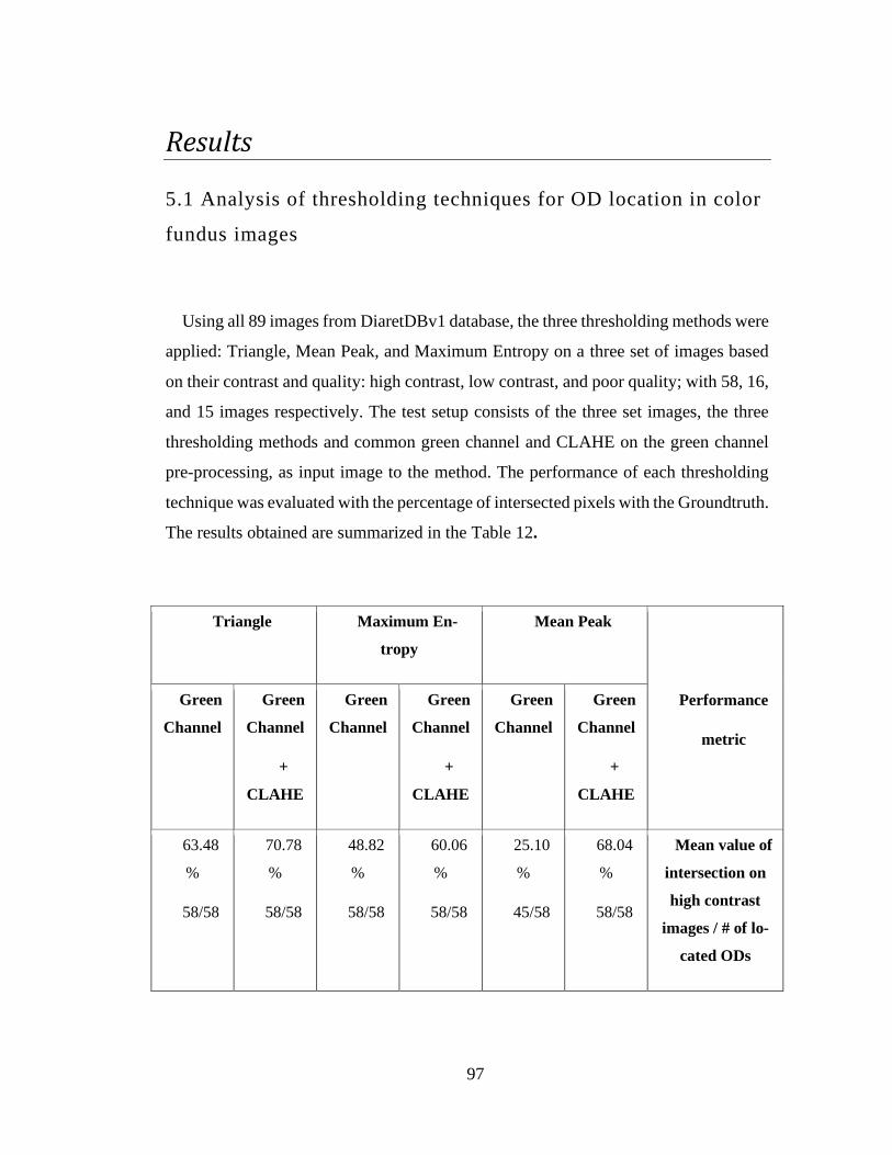
97
Results
5.1 Analysis of thresholding techniques for OD location in color
fundus images
Using all 89 images from DiaretDBv1 database, the three thresholding methods were
applied: Triangle, Mean Peak, and Maximum Entropy on a three set of images based
on their contrast and quality: high contrast, low contrast, and poor quality; with 58, 16,
and 15 images respectively. The test setup consists of the three set images, the three
thresholding methods and common green channel and CLAHE on the green channel
pre-processing, as input image to the method. The performance of each thresholding
technique was evaluated with the percentage of intersected pixels with the Groundtruth.
The results obtained are summarized in the Table 12.
Triangle Maximum En-
tropy
Mean Peak
Performance
metric
Green
Channel
Green
Channel
+
CLAHE
Green
Channel
Green
Channel
+
CLAHE
Green
Channel
Green
Channel
+
CLAHE
63.48
%
58/58
70.78
%
58/58
48.82
%
58/58
60.06
%
58/58
25.10
%
45/58
68.04
%
58/58
Mean value of
intersection on
high contrast
images / # of lo-
cated ODs
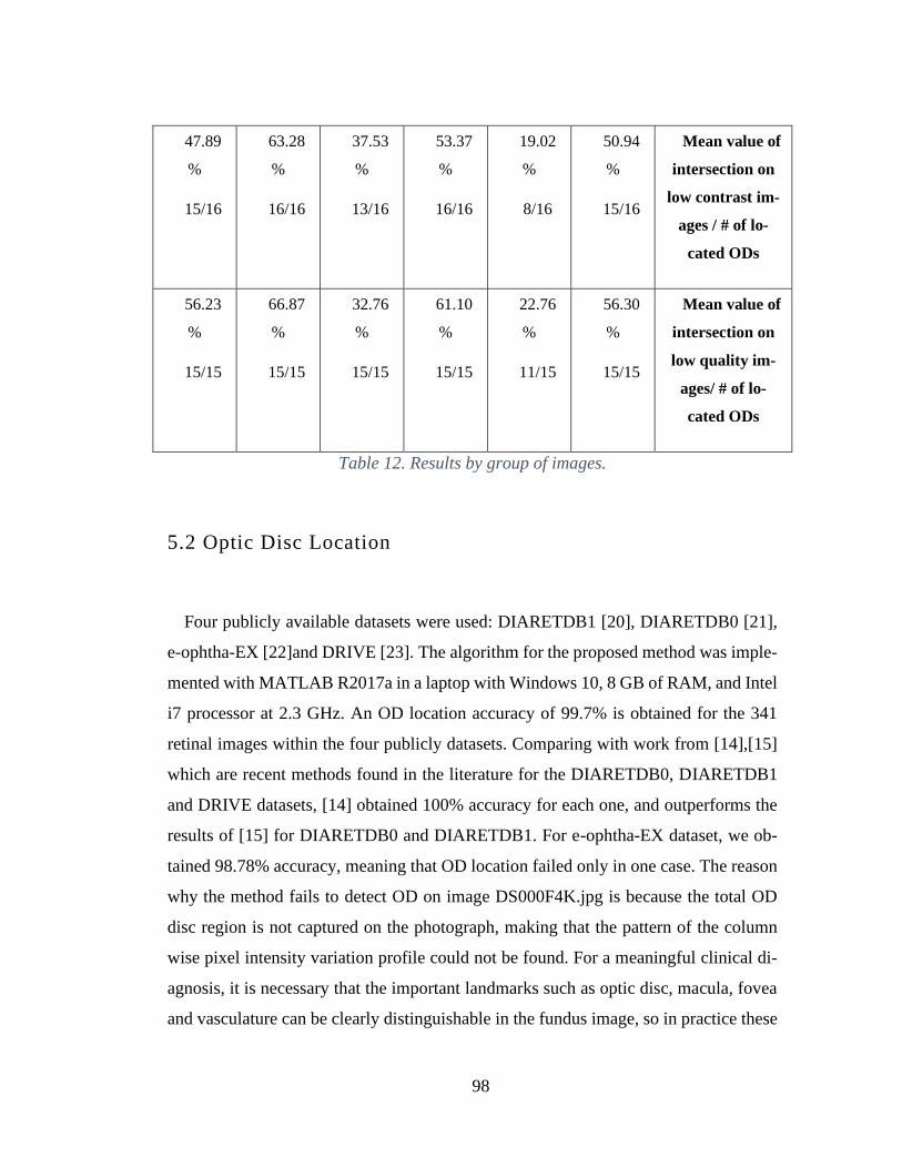
98
47.89
%
15/16
63.28
%
16/16
37.53
%
13/16
53.37
%
16/16
19.02
%
8/16
50.94
%
15/16
Mean value of
intersection on
low contrast im-
ages / # of lo-
cated ODs
56.23
%
15/15
66.87
%
15/15
32.76
%
15/15
61.10
%
15/15
22.76
%
11/15
56.30
%
15/15
Mean value of
intersection on
low quality im-
ages/ # of lo-
cated ODs
Table 12. Results by group of images.
5.2 Optic Disc Location
Four publicly available datasets were used: DIARETDB1 [20], DIARETDB0 [21],
e-ophtha-EX [22]and DRIVE [23]. The algorithm for the proposed method was imple-
mented with MATLAB R2017a in a laptop with Windows 10, 8 GB of RAM, and Intel
i7 processor at 2.3 GHz. An OD location accuracy of 99.7% is obtained for the 341
retinal images within the four publicly datasets. Comparing with work from [14],[15]
which are recent methods found in the literature for the DIARETDB0, DIARETDB1
and DRIVE datasets, [14] obtained 100% accuracy for each one, and outperforms the
results of [15] for DIARETDB0 and DIARETDB1. For e-ophtha-EX dataset, we ob-
tained 98.78% accuracy, meaning that OD location failed only in one case. The reason
why the method fails to detect OD on image DS000F4K.jpg is because the total OD
disc region is not captured on the photograph, making that the pattern of the column
wise pixel intensity variation profile could not be found. For a meaningful clinical di-
agnosis, it is necessary that the important landmarks such as optic disc, macula, fovea
and vasculature can be clearly distinguishable in the fundus image, so in practice these
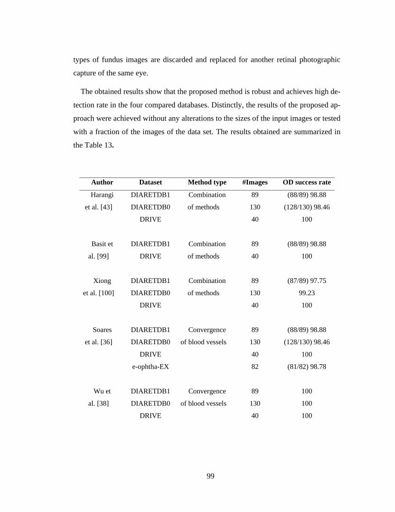
99
types of fundus images are discarded and replaced for another retinal photographic
capture of the same eye.
The obtained results show that the proposed method is robust and achieves high de-
tection rate in the four compared databases. Distinctly, the results of the proposed ap-
proach were achieved without any alterations to the sizes of the input images or tested
with a fraction of the images of the data set. The results obtained are summarized in
the Table 13.
Author Dataset Method type #Images OD success rate
Harangi
et al. [43]
DIARETDB1
DIARETDB0
DRIVE
Combination
of methods
89
130
40
(88/89) 98.88
(128/130) 98.46
100
Basit et
al. [99]
DIARETDB1
DRIVE
Combination
of methods
89
40
(88/89) 98.88
100
Xiong
et al. [100]
DIARETDB1
DIARETDB0
DRIVE
Combination
of methods
89
130
40
(87/89) 97.75
99.23
100
Soares
et al. [36]
DIARETDB1
DIARETDB0
DRIVE
e-ophtha-EX
Convergence
of blood vessels
89
130
40
82
(88/89) 98.88
(128/130) 98.46
100
(81/82) 98.78
Wu et
al. [38]
DIARETDB1
DIARETDB0
DRIVE
Convergence
of blood vessels
89
130
40
100
100
100
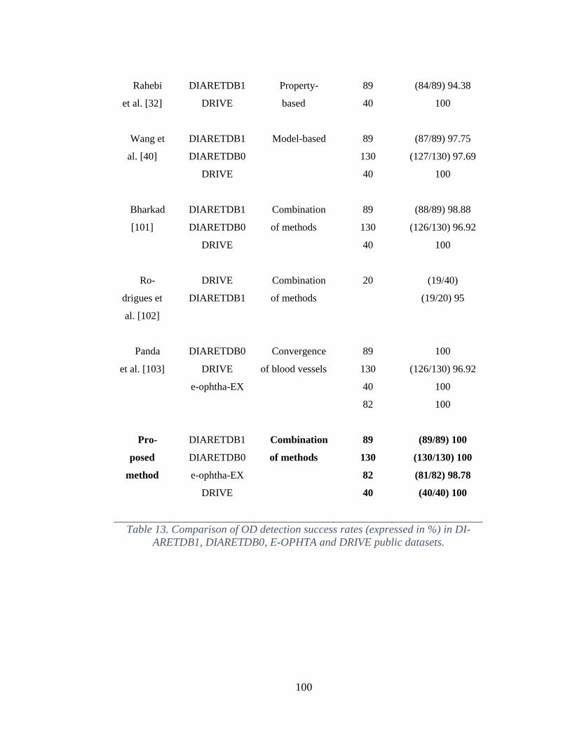
100
Rahebi
et al. [32]
Wang et
al. [40]
Bharkad
[101]
Ro-
drigues et
al. [102]
Panda
et al. [103]
DIARETDB1
DRIVE
DIARETDB1
DIARETDB0
DRIVE
DIARETDB1
DIARETDB0
DRIVE
DRIVE
DIARETDB1
DIARETDB0
DRIVE
e-ophtha-EX
Property-
based
Model-based
Combination
of methods
Combination
of methods
Convergence
of blood vessels
89
40
89
130
40
89
130
40
20
89
130
40
82
(84/89) 94.38
100
(87/89) 97.75
(127/130) 97.69
100
(88/89) 98.88
(126/130) 96.92
100
(19/40)
(19/20) 95
100
(126/130) 96.92
100
100
Pro-
posed
method
DIARETDB1
DIARETDB0
e-ophtha-EX
DRIVE
Combination
of methods
89
130
82
40
(89/89) 100
(130/130) 100
(81/82) 98.78
(40/40) 100
Table 13. Comparison of OD detection success rates (expressed in %) in DI-
ARETDB1, DIARETDB0, E-OPHTA and DRIVE public datasets.
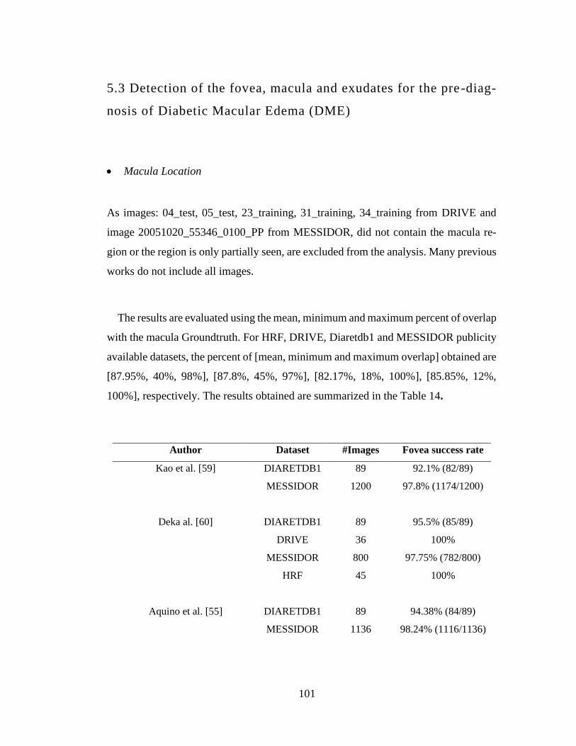
101
5.3 Detection of the fovea, macula and exudates for the pre-diag-
nosis of Diabetic Macular Edema (DME)
• Macula Location
As images: 04_test, 05_test, 23_training, 31_training, 34_training from DRIVE and
image 20051020_55346_0100_PP from MESSIDOR, did not contain the macula re-
gion or the region is only partially seen, are excluded from the analysis. Many previous
works do not include all images.
The results are evaluated using the mean, minimum and maximum percent of overlap
with the macula Groundtruth. For HRF, DRIVE, Diaretdb1 and MESSIDOR publicity
available datasets, the percent of [mean, minimum and maximum overlap] obtained are
[87.95%, 40%, 98%], [87.8%, 45%, 97%], [82.17%, 18%, 100%], [85.85%, 12%,
100%], respectively. The results obtained are summarized in the Table 14.
Author Dataset #Images Fovea success rate
Kao et al. [59] DIARETDB1
MESSIDOR
89
1200
92.1% (82/89)
97.8% (1174/1200)
Deka al. [60]
DIARETDB1
DRIVE
MESSIDOR
HRF
89
36
800
45
95.5% (85/89)
100%
97.75% (782/800)
100%
Aquino et al. [55] DIARETDB1
MESSIDOR
89
1136
94.38% (84/89)
98.24% (1116/1136)
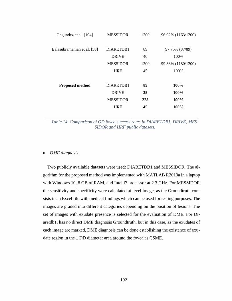
102
Gegundez et al. [104]
Balasubramanian et al. [58]
MESSIDOR
DIARETDB1
DRIVE
MESSIDOR
HRF
1200
89
40
1200
45
96.92% (1163/1200)
97.75% (87/89)
100%
99.33% (1180/1200)
100%
Proposed method DIARETDB1
DRIVE
MESSIDOR
HRF
89
35
225
45
100%
100%
100%
100%
Table 14. Comparison of OD fovea success rates in DIARETDB1, DRIVE, MES-
SIDOR and HRF public datasets.
• DME diagnosis
Two publicly available datasets were used: DIARETDB1 and MESSIDOR. The al-
gorithm for the proposed method was implemented with MATLAB R2019a in a laptop
with Windows 10, 8 GB of RAM, and Intel i7 processor at 2.3 GHz. For MESSIDOR
the sensitivity and specificity were calculated at level image, as the Groundtruth con-
sists in an Excel file with medical findings which can be used for testing purposes. The
images are graded into different categories depending on the position of lesions. The
set of images with exudate presence is selected for the evaluation of DME. For Di-
aretdb1, has no direct DME diagnosis Groundtruth, but in this case, as the exudates of
each image are marked, DME diagnosis can be done establishing the existence of exu-
date region in the 1 DD diameter area around the fovea as CSME.
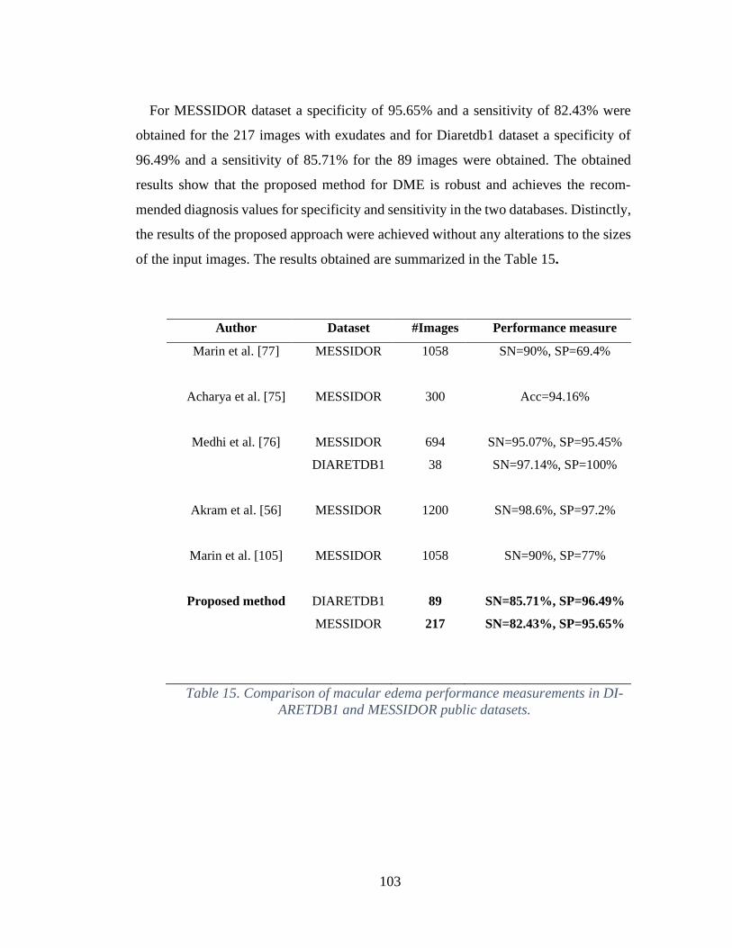
103
For MESSIDOR dataset a specificity of 95.65% and a sensitivity of 82.43% were
obtained for the 217 images with exudates and for Diaretdb1 dataset a specificity of
96.49% and a sensitivity of 85.71% for the 89 images were obtained. The obtained
results show that the proposed method for DME is robust and achieves the recom-
mended diagnosis values for specificity and sensitivity in the two databases. Distinctly,
the results of the proposed approach were achieved without any alterations to the sizes
of the input images. The results obtained are summarized in the Table 15.
Author Dataset #Images Performance measure
Marin et al. [77]
MESSIDOR 1058 SN=90%, SP=69.4%
Acharya et al. [75] MESSIDOR
300
Acc=94.16%
Medhi et al. [76]
Akram et al. [56]
Marin et al. [105]
MESSIDOR
DIARETDB1
MESSIDOR
MESSIDOR
694
38
1200
1058
SN=95.07%, SP=95.45%
SN=97.14%, SP=100%
SN=98.6%, SP=97.2%
SN=90%, SP=77%
Proposed method DIARETDB1
MESSIDOR
89
217
SN=85.71%, SP=96.49%
SN=82.43%, SP=95.65%
Table 15. Comparison of macular edema performance measurements in DI-
ARETDB1 and MESSIDOR public datasets.

104
Conclusions and Discussion
6.1 Discussion
• Optic disc location
The proposed optic disc method has four main stages: OD pixel region candidate
generation, promising OD regions detection, promising candidate features extraction,
and classification. Given that datasets have images with non-uniform illumination, re-
gional intensity variations are found along the fundus image, this to overcome the well-
known unreliable use of a global high intensity threshold to locate promising OD re-
gions. That led us to use a window partitioning approach for the extraction of local OD
candidate regions. Recapitulating, the proposed approach consists of a top-down ap-
proach, from a group of high intensity local regions with coarse level features to finer
features on extended regions with minimum requirements on size and intensity distri-
bution, which form the most promising OD regions. A model for the column wise pixel
intensity variation is proposed, and the features are defined according to the expected
OD pattern on the column wise pixel intensity variation model: presence of a Left Lobe
(LL), a Right Lobe (RL) and Vasculature (V) between them, and distances from LL to
V and V to RL. Classification is done accordingly to the presence of the LL-V-RL
pattern. The proposed algorithm can be negatively affected if the retinal vasculature is
not distinguishable, i.e. vessels belonging to the main arcades have low contrast or are
quite difficult to observe. On the OD pixel region candidate generation stage, the in-
clusion of the OD true region as candidate depends on OD true region having a relevant
local intensity with respect of another bright regions or artifacts that might be present
on the windowed section of the image. Another source of error could be when the ver-
tical vessels that emerge from the OD are either not present or exhibit a low contrast in
comparison with other vertical vessels in other regions of the retina, this could lead to
an incorrect OD classification. For the correct classification of OD candidate regions
using the model for the column wise pixel intensity variations across the optic disc it
105
is necessary that the majority of the actual OD region will be present on the analyzed
fundus image.
• Macula location
The algorithm initially searches for the fovea region, macula center, with prior in-
formation that it is the darkest intensity region. A threshold is locally defined using k-
means clustering. For the challenging images including those with the presence of large
hemorrhages and low contrast, an alternative approach is applied based on the fact that
fovea center is estimated to be at a constant distance of approximately 2.5 OD diameter
of OD center and that is a region devoid of retinal blood vessels.
We identified two main reasons for the failure in successfully detecting macula in
this study: (1) failure in correctly determining the macula search region (2) failure in
determining macula candidate. The first failure is associated with variations on the
standard distance between the OD center and the macula center given by the expression
2.5 OD diameter pixels which may be inaccurate in some cases. The second failure is
associated with the images where macula is not present or partially present, affecting
the proposed features. However, this kind of images in clinical practice should be re-
taken, as they lack quality for diagnosis.
• DME pre-diagnosis
Exudates are segmented based on their high intensity along with their sharp edges
and high contrast characteristics. From the observation of the patterns of exudates le-
sions, we determined that exudates intensity variation present a gradual shift in con-
centric form, going from high intensity values at its center to lower values as back-
ground is reached. Aiming to represent this pattern, a contour map of the image was
calculated. Exudate candidates with this pattern are further processed. Four
106
characteristics were extracted for each candidate exudate region: maximum green in-
tensity value of the pixels conforming the candidate region, mean green intensity value
of the pixels conforming the candidate region, the number of different gray levels found
in the region in the green channel and the maximum border intensity value that was
calculated extending the candidate region and applying the range filter. Based on these
four characteristics, a series of systematic tests were conducted, aiming to find the
range values for the combination of characteristics with which the target sensitivity and
specificity are achieved, 80% and 95% respectively.
6.2 Conclusions
In this work, several advancements in retinal image processing aimed toward im-
proving the state-of-the-art in automated screening were developed: image enhance-
ment, retinal structures location, lesion detection and disease classification.
A solution for the location of the optic disc and macula, exudate detection and Dia-
betic Macular edema pre-diagnosis using color images of eye fundus was proposed and
validated using multiple public image databases with different resolutions and achiev-
ing competent results with respect of the state-of-the-art approaches, achieving the
main goal of this work. The important aspects of the proposed solution include: low
computational cost, image resolution independence and robustness. According to the
achieved performance of the proposed method and its simplicity, has the potential
of assessing the integration into a retinal disease pre-screening tool.
A new approach for the location of the optic disc in fundus images was developed.
The approach proved to be simple and reliable; especially for challenging images, in-
cluding images with poor illumination, pathological changes, with dark OD due to un-
even illumination and low contrast, with partial OD section and images with bright

107
exudates whose size and intensity are similar to OD. The robustness of the proposed
technique is guaranteed by evaluating the method in four publicly-available datasets:
DIARETDB1, DIARETDB0, e-ophtha-EX and DRIVE, obtaining a disc detection suc-
cess rate of 100%, 100%, 98.78% and 100% respectively. Distinctly, since anatomical
features calculated are relative to image’s original resolution, the results of the pro-
posed approach were achieved without any transformations to the sizes of the input
images, making our detection algorithm scalable in terms of image resolution. Unlike
most approaches, since no training was required for the classification stage, no addi-
tional datasets are needed for this task and the test results are calculated using all im-
ages of the datasets, versus previous works that use typically 30% of the images to test.
For macula location, a novel methodology combining anatomical and visual feature-
based criteria is proposed. As the methods that only employ either only the visual or
the anatomical features could fail in presence of lesions occluding the macula, the pro-
posed algorithm can overcome these problems of failure or incorrect detection using
all the macula characteristics i.e. low intensity, lack of blood vessels and distance with
respect to OD. The results were evaluated using the mean, minimum and maximum
percent of overlap with the macula Groundtruth. For HRF, DRIVE, Diaretdb1 and
MESSIDOR publicity available datasets, the percent of [mean, minimum and maxi-
mum overlap] obtained were [87.95%, 40%, 98%], [87.8%, 45%, 97%], [82.17%, 18%,
100%], [85.85%, 12%, 100%], respectively. In addition, the proposed approach is in-
dependent of image resolution, since the anatomical constraints and features extracted
are relative to OD estimation. Considering the results obtained, the proposed method
yielded high detection accuracy along with robustness in macula location. The pro-
posed method could be used as a tool to be integrated into a complete prescreening
system for early retinal disease detection.
108
For Diabetic Macular Edema (DME) diagnosis, we developed a methodology for
grading the risk of DME based on exudate detection in fundus images. Our proposed
approach consists on using the coordinates of macula previously acquired and the dis-
tance of exudates from macula, the input fundus is graded in two categories, Non
CSME and CSME. For MESSIDOR dataset a specificity of 95.65% and a sensitivity
of 82.43% were obtained for the 217 images with exudates and for Diaretdb1 dataset a
specificity of 96.49% and a sensitivity of 85.71% for the 89 images were obtained. The
obtained results show that the proposed method for DME is robust and achieves the
recommended diagnosis values for specificity and sensitivity in the two databases. Dis-
tinctly, the results of the proposed approach were achieved without any alterations to
the sizes of the input images. The results demonstrated that the proposed methodology
can be used in an automated medical system for the pre-diagnosis of diabetic macular
edema.
6.3 Contributions
The presented approach in this thesis could comprise a model for the development
of a system that can be used as a pre-diagnostic tool for retinal diseases. The proposed
approach is less computationally demanding than compared to the commonly used op-
erations for the state-of-the-art methods. The development of an automatic pre-diagno-
sis system in the future could reduce the future gap between the number of diabetic
patients and the number of ophthalmologists worldwide and become an economical
preliminary ophthalmologic diagnostic medium that facilitates the way in which rou-
tine preventive examinations are done. In this way the ophthalmologist’s workload re-
lated to diabetic patients could be alleviated and the economic and time costs can be
reduced, making eye screening affordable and facilitating that patients take the exam
at least twice a year as it is recommended.
109
Considering that OD could present similar characteristics with some signs of diabetic
retinopathy, the proposed OD location approach can be applied to remove the OD re-
gion before the detection of these signs, avoiding the possibility of erroneously classi-
fying OD sections as pathology lesions in automated diabetic retinopathy (DR) screen-
ing.
Also, the design of a profile model of OD intensity variations was contributed. This
model represents the nature of the variation of the pixel’s intensities of the OD region
which makes it tolerant to color variability in fundus images. Also, this model can be
easily scaled for any resolution. This was verified when testing this model with four
databases with different resolutions. Resolution independence is of great importance
specially for large scale screening programs, where the images to be analyzed come
from different fundus cameras thus having variety of resolutions.
6.4 Future work
There are numerous image processing techniques with different approaches that
could possibly solve the problems posed with better results, but they are mostly com-
plex, with high processing time, dataset dependent, and image resolution dependent.
Some proposals that could be implemented in the future are:
Develop a module that can estimate the image quality, so that a minimum quality
could be established for the fundus color retinal image of the patient as appropriate for
automatic diagnosis. This problem could also be solved through quality control in the
process of acquisition of the fundus image.
110
The development of a database with their respective Groundtruth where the lesions
and retinal structures are marked as accurately as possible. Facilitating the evaluation
and comparison of the proposed methodologies. In this way, it can become a standard
database with which different methods can be compared in a simple way.
Add other pre-diagnoses of retinal diseases to the system. With the proposed optic
disc approach, an automated method for grading glaucoma could be developed locating
accurately the optic disc cup and the optic disc rim, as glaucoma is diagnosed based on
the ratio relation between them.
111
References
[1] S. Resnikoff, W. Felch, T. Gauthier, and B. Spivey, “The number of
ophthalmologists in practice and training worldwide : a growing gap despite
more than 200 000 practitioners,” Britih Journal of Ophthalmology, pp. 1–5,
2012, doi: 10.1136/bjophthalmol-2011-301378.
[2] S. H. P. Andrew Stokes, “Deaths Attributable to Diabetes in the United States:
Comparison of Data Sources and Estimation Approaches,” PLoS ONE, 2017.
[3] IAPB, “Diabetic retinopathy: Challenges and opportunities,” 2016. [Online].
Available: http://www.iapb.org/vision-2020/what-is-avoidable-
blindness/diabetic-retinopathy. [Accessed: 08-Feb-2017].
[4] I. N. de S. P. de Mexico, “Diabetes, causa principal de muerte en México.”
[Online]. Available: https://www.insp.mx/presencia-insp/3877-presencia-
insp.html. [Accessed: 08-Feb-2017].
[5] K. V. K. Narasimhan, V.C. Neha, “An efficient automated system for detection
of diabetic retinopathy from fundus images using support vector machine and
bayesian classifiers,” in International Conference on Computing, Electronics
and Electrical Technologies [ICCEET], 2012, pp. 964–969.
[6] M. S. de Salud, “Diagnóstico y tratamiento de retinopatía diabética,” 2015.
[7] W. H. Organization, “country profiles,” 2016.
[8] W. H. J. Díaz, “Diabetes and Cause-Specific Mortality in Mexico City,” The
new england journal of medicine, 2016.
[9] B. D. Association, “Retinal photography screening for diabetic eye disease,”
1994.
[10] B. Liesenfeld et al., “A telemedical approach to the screening of diabetic
retinopathy: Digital fundus photography,” Diabetes Care, vol. 23, no. 3, pp.
112
345–348, 2000, doi: 10.2337/diacare.23.3.345.
[11] Spector RH, “The Pupils,” in Clinical Methods: The History, Physical, and
Laboratory Examinations, 1990, p. Chapter 58.
[12] M. Foracchia, E. Grisan, and A. Ruggeri, “Luminosity and contrast
normalization in retinal images,” Medical Image Analysis, vol. 9, no. 3, pp. 179–
190, 2005, doi: 10.1016/j.media.2004.07.001.
[13] T. Kauppi, “Eye fundus image analysis for automatic detection of diabetic
retinopathy,” 2010.
[14] A. Fadzil M. Hani and H. Adi Nugroho, “Retinal vasculature enhancement using
independent component analysis,” Journal of Biomedical Science and
Engineering, vol. 02, no. 07, pp. 543–549, 2009, doi: 10.4236/jbise.2009.27079.
[15] T. Roy, Handbook of Retinal Screening in Diabetes: Diagnosis and
Management. .
[16] R. J. Winder, P. J. Morrow, I. N. Mcritchie, J. R. Bailie, and P. M. Hart,
“Algorithms for digital image processing in diabetic retinopathy,” Computerized
Medical Imaging and Graphics, vol. 33, pp. 608–622, 2009, doi:
10.1016/j.compmedimag.2009.06.003.
[17] A. Pardo and G. Sapiro, “Visualization of high dynamic range images,” IEEE
Transactions on Image Processing, vol. 12, no. 6, pp. 639–647, 2003, doi:
10.1109/TIP.2003.812373.
[18] R. Wallis, “An approach to the space variant restoration and enhancement of
images,” in Current mathematical problems in imaging science, 1976, pp. 329–
340.
[19] W. Gonzalez, Digital Image Processing. .
[20] T. B. Markham R. Osareh A. Mirmehdi M., “Automated identification of
diabetic retinal exudates in digital color images,” Brithish Journal of

113
Ophthalmology, vol. 87, pp. 1220–1230, 2003.
[21] A. M. Gooch B. Shirley P. Reinhard E., “Color transfer between images,” IEEE
Computer Graphics and Applications, vol. 21, pp. 34–41, 2001.
[22] S. B. Sakchai V. Nattapol W. Akara S. Bunyarit U., “Fine exudate detection
using morphological approach,” International journal of applied biomedical
engineering, vol. 1, no. 1, pp. 45–50, 2010.
[23] A. M. N. Allam, A. A. H. Youssif, and A. Z. Ghalwash, “Automatic
segmentation of optic disc in eye fundus images: A survey,” Electronic Letters
on Computer Vision and Image Analysis, vol. 14, no. 1, pp. 1–20, 2015, doi:
10.5565/rev/elcvia.680.
[24] M. Ortega, M. G. Penedo, J. Rouco, N. Barreira, and M. J. Carreira, “Retinal
Verification Using a Feature Points-Based Biometric Pattern,” EURASIP
Journal on Advances in Signal Processing, vol. 2009, no. 1, pp. 1–13, 2009, doi:
10.1155/2009/235746.
[25] Y. Jiang, “Blood vessel tracking in retinal images,” in Proceedings of Image and
Vision Computing, 2007, vol. 1, pp. 126–131.
[26] I. W. R. A. Abdel-Ghafar, T. Morris, T. Ritchings, “Progress Towards
Automated Detection and Characterisation of the Optic Disk in Glaucoma and
Diabetic Retinopathy,” Medical Informatics and the Internet in Medicine, vol.
32, no. 1, pp. 19–25, 2007.
[27] B. G. Meindert Niemeijer, Michael D. Abràmoff, “Fast Detection of the Optic
Disc and Fovea in Color Fundus Photographs,” Medical Image Analysis, vol.
13, no. 6, pp. 859–870, 2009, doi: 10.1016/j.pestbp.2011.02.012.Investigations.
[28] R. J. Qureshi, L. Kovacs, B. Harangi, B. Nagy, T. Peto, and A. Hajdu,
“Combining algorithms for automatic detection of optic disc and macula in
fundus images,” Computer Vision and Image Understanding, vol. 116, no. 1,
pp. 138–145, 2012, doi: 10.1016/j.cviu.2011.09.001.
114
[29] A. V. Deshmukh, T. G. Patil, S. S. Patankar, and J. V. Kulkarni, “Features based
classification of hard exudates in retinal images,” 2015 International
Conference on Advances in Computing, Communications and Informatics,
ICACCI 2015, pp. 1652–1655, 2015, doi: 10.1109/ICACCI.2015.7275850.
[30] C. A. G. Sergio Bonafonte Royo, retinopatía diabética. Elsevier España,
isbn:9788481748512.
[31] R. Pourreza-Shahri, M. Tavakoli, and N. Kehtarnavaz, “Computationally
efficient optic nerve head detection in retinal fundus images,” Biomedical Signal
Processing and Control, vol. 11, no. 1, pp. 63–73, 2014, doi:
10.1016/j.bspc.2014.02.011.
[32] J. Rahebi and F. Hardalac, “A new approach to optic disc detection in human
retinal images using the firefly algorithm,” Medical & Biological Engineering
& Computing, vol. 54, no. 2, pp. 453–461, 2015, doi: 10.1007/s11517-015-
1330-7.
[33] X.-S. Yang, “Firefly Algorithm,” in Nature-Inspired Metaheuristics Algorithms,
2nd ed., Frome: Luniver Press, 2010, pp. 81–89.
[34] M. S. Haleem, L. Han, J. van Hemert, and B. Li, “Automatic extraction of retinal
features from colour retinal images for glaucoma diagnosis: A review,”
Computerized Medical Imaging and Graphics, vol. 37, no. 7, pp. 581–596, 2013,
doi: 10.1016/j.compmedimag.2013.09.005.
[35] M. Foracchia, E. Grisan, and A. Ruggeri, “Detection of optic disc in retinal
images by means of a geometrical model of vessel structure,” IEEE
Transactions on Medical Imaging, vol. 23, no. 10, pp. 1189–1195, 2004, doi:
10.1109/TMI.2004.829331.
[36] I. Soares, M. Castelo-Branco, and A. M. G. Pinheiro, “Optic Disc Localization
in Retinal Images Based on Cumulative Sum Fields,” IEEE Journal of
Biomedical and Health Informatics, vol. 20, no. 2, pp. 574–585, 2016, doi:
115
10.1109/JBHI.2015.2392712.
[37] D. Marin, M. E. Gegundez-Arias, A. Suero, and J. M. Bravo, “Obtaining optic
disc center and pixel region by automatic thresholding methods on
morphologically processed fundus images,” Computer Methods and Programs
in Biomedicine, vol. 118, no. 2, pp. 173–185, 2015, doi:
10.1016/j.cmpb.2014.11.003.
[38] X. Wu, B. Dai, and W. Bu, “Optic Disc Localization Using Directional Models,”
IEEE Transactions on Image Processing, vol. 25, no. 9, pp. 4433–4442, 2016,
doi: 10.1109/TIP.2016.2590838.
[39] B. Dashtbozorg, A. M. Mendonca, and A. Campilho, “Optic disc segmentation
using the sliding band filter.,” Computers in biology and medicine, vol. 56, pp.
1–12, 2015, doi: 10.1016/j.compbiomed.2014.10.009.
[40] C. Wang, D. Kaba, and Y. Li, “Level Set Segmentation of Optic Discs from
Retinal Images,” Journal of Medical and Bioengineering, vol. 4, no. 3, pp. 213–
220, 2015, doi: 10.12720/jomb.4.3.213-220.
[41] M. C. V. S. Mary, E. B. Rajsingh, J. K. K. Jacob, D. Anandhi, U. Amato, and S.
E. Selvan, “An empirical study on optic disc segmentation using an active
contour model,” Biomedical Signal Processing and Control, vol. 18, pp. 19–29,
2015, doi: 10.1016/j.bspc.2014.11.003.
[42] J. M. Molina-Casado, E. J. Carmona, and J. García-Feijoó, “Fast detection of
the main anatomical structures in digital retinal images based on intra- and inter-
structure relational knowledge,” Computer Methods and Programs in
Biomedicine, vol. 149, pp. 55–68, 2017, doi: 10.1016/j.cmpb.2017.06.022.
[43] B. Harangi and A. Hajdu, “Detection of the optic disc in fundus images by
combining probability models,” Computers in Biology and Medicine, vol. 65,
pp. 10–24, 2015, doi: 10.1016/j.compbiomed.2015.07.002.
[44] F. Ren, W. Li, J. Yang, H. Geng, and D. Zhao, “Automatic optic disc localization
116
and segmentation in retinal images by a line operator and level sets,” Technology
and Health Care, vol. 24, pp. S767–S776, 2016, doi: 10.3233/THC-161206.
[45] A. Basit and M. M. Fraz, “Optic disc detection and boundary extraction in retinal
images.,” Applied optics, vol. 54, no. 11, pp. 3440–7, 2015, doi:
10.1364/AO.54.003440.
[46] L. Xiong and H. Li, “An approach to locate optic disc in retinal images with
pathological changes,” Computerized Medical Imaging and Graphics, vol. 47,
pp. 40–50, 2016, doi: 10.1016/j.compmedimag.2015.10.003.
[47] M. Haloi, S. Dandapat, and R. Sinha, “An Unsupervised Method for Detection
and Validation of The Optic Disc and The Fovea,” Computer Vision and Pattern
Recognition, pp. 1–8, 2016.
[48] D. Díaz-Pernil, I. Fondón, F. Peña-Cantillana, and M. A. Gutiérrez-Naranjo,
“Fully automatized parallel segmentation of the optic disc in retinal fundus
images,” Pattern Recognition Letters, vol. 0, pp. 1–9, 2016, doi:
10.1016/j.patrec.2016.04.025.
[49] Z. Fan et al., “Optic Disk Detection in Fundus Image Based on Structured
Learning,” IEEE Journal of Biomedical and Health Informatics, vol. 22, no. 1,
pp. 224–234, 2018, doi: 10.1109/JBHI.2017.2723678.
[50] O. Faust, R. Acharya U., E. Y. K. Ng, K. H. Ng, and J. S. Suri, “Algorithms for
the automated detection of diabetic retinopathy using digital fundus images: A
review,” Journal of Medical Systems, vol. 36, no. 1, pp. 145–157, 2012, doi:
10.1007/s10916-010-9454-7.
[51] L. P. Aiello et al., “Diabetic retinopathy technical review,” Diabetes Care, vol.
21, pp. 143–156, 1998.
[52] J. W. Yau et al., “Global prevalence and major risk factors of diabetic
retinopathy,” Diabetes Care, vol. 3, no. 35, pp. 556–564, 2012.
117
[53] N. Bhagat, R. A. Grigorian, A. Tutela, and M. A. Zarbin, “Diabetic macular
edema: pathogenesis and treatment,” Surv. Ophthalmol., vol. 54, no. 1, pp. 1–
32, 2009.
[54] M. R. K. Mookiah et al., “Application of different imaging modalities for
diagnosis of Diabetic Macular Edema: A review,” Computers in Biology and
Medicine, vol. 66, pp. 295–315, 2015, doi: 10.1016/j.compbiomed.2015.09.012.
[55] A. Aquino, “Establishing the macular grading grid by means of fovea centre
detection using anatomical-based and visual-based features,” Computers in
Biology and Medicine, vol. 55, pp. 61–73, 2014, doi:
10.1016/j.compbiomed.2014.10.007.
[56] M. U. Akram, A. Tariq, S. A. Khan, and M. Y. Javed, “Automated detection of
exudates and macula for grading of diabetic macular edema,” Computer
Methods and Programs in Biomedicine, vol. 114, no. 2, pp. 141–152, 2014, doi:
10.1016/j.cmpb.2014.01.010.
[57] M. U. Akram and S. A. Khan, “Multilayered thresholding-based blood vessel
segmentation for screening of diabetic retinopathy,” Engineering with
Computers, vol. 29, no. 2, pp. 165–173, 2013, doi: 10.1007/s00366-011-0253-
7.
[58] R. GeethaRamani and L. Balasubramanian, “Macula segmentation and fovea
localization employing image processing and heuristic based clustering for
automated retinal screening,” Computer Methods and Programs in Biomedicine,
vol. 160, pp. 153–163, 2018, doi: 10.1016/j.cmpb.2018.03.020.
[59] E. F. Kao, P. C. Lin, M. C. Chou, T. S. Jaw, and G. C. Liu, “Automated detection
of fovea in fundus images based on vessel-free zone and adaptive Gaussian
template,” Computer Methods and Programs in Biomedicine, vol. 117, no. 2,
pp. 92–103, 2014, doi: 10.1016/j.cmpb.2014.08.003.
[60] D. Deka, J. P. Medhi, and S. R. Nirmala, “Detection of macula and fovea for
118
disease analysis in color fundus images,” 2015 IEEE 2nd International
Conference on Recent Trends in Information Systems, ReTIS 2015 -
Proceedings, pp. 231–236, 2015, doi: 10.1109/ReTIS.2015.7232883.
[61] A. Aquino, M. E. Gegúndez-Arias, and D. Marín, “Detecting the Optic Disc
Boundary in Digital Fundus Feature Extraction Techniques,” Ieee Transactions
on Medical Imaging, vol. 29, no. 11, pp. 1860–1869, 2010.
[62] D. Marín, A. Aquino, M. E. Gegúndez-Arias, and J. M. Bravo, “A new
supervised method for blood vessel segmentation in retinal images by using
gray-level and moment invariants-based features,” IEEE Transactions on
Medical Imaging, vol. 30, no. 1, pp. 146–158, 2011, doi:
10.1109/TMI.2010.2064333.
[63] N. Y. Garaibeh, M. a. Al-Smadi, and M. Al-Jarrah, “Automatic Exudate
Detection Using Eye Fundus Image Analysis Due to Diabetic Retinopathy,”
Computer and Information Science, vol. 7, no. 2, pp. 48–55, 2014, doi:
10.5539/cis.v7n2p48.
[64] E. Imani and H. R. Pourreza, “A novel method for retinal exudate segmentation
using signal separation algorithm,” Computer Methods and Programs in
Biomedicine, vol. 133, pp. 195–205, 2016, doi: 10.1016/j.cmpb.2016.05.016.
[65] B. Harangi and A. Hajdu, “Automatic exudate detection by fusing multiple
active contours and regionwise classification,” Computers in Biology and
Medicine, vol. 54, pp. 156–171, 2014, doi: 10.1016/j.compbiomed.2014.09.001.
[66] M. Esmaeili, H. Rabbani, A. M. Dehnavi, and A. Dehghani, “Automatic
detection of exudates and optic disk in retinal images using curvelet transform,”
IET Image Processing, vol. 6, no. 7, pp. 1005–1013, 2012, doi: 10.1049/iet-
ipr.2011.0333.
[67] U. M. Akram and S. A. Khan, “Automated detection of dark and bright lesions
in retinal images for early detection of diabetic retinopathy,” Journal of Medical
119
Systems, vol. 36, no. 5, pp. 3151–3162, 2012, doi: 10.1007/s10916-011-9802-2.
[68] C. Pereira, L. Gonçalves, and M. Ferreira, “Exudate segmentation in fundus
images using an ant colony optimization approach,” Information Sciences, vol.
296, no. October, pp. 14–24, 2015, doi: 10.1016/j.ins.2014.10.059.
[69] A. Elbalaoui, M. Boutaounte, H. Faouzi, M. Fakir, and A. Merbouha,
“Segmentation and detection of diabetic retinopathy exudates,” International
Conference on Multimedia Computing and Systems -Proceedings, vol. 91, no.
16, pp. 171–178, 2014, doi: 10.1109/ICMCS.2014.6911368.
[70] R. Bhargavi V and R. K. Senapati, “Bright Lesion Detection in Color Fundus
Images Based on Texture Features,” Bulletin of Electrical Engineering and
Informatics, vol. 5, no. 1, pp. 92–100, 2016, doi: 10.11591/eei.v5i1.553.
[71] S. Lahmiri and M. Boukadoum, “Automated detection of circinate exudates in
retina digital images using empirical mode decomposition and the entropy and
uniformity of the intrinsic mode functions,” Biomedizinische Technik, vol. 59,
no. 4, pp. 357–366, 2014, doi: 10.1515/bmt-2013-0082.
[72] S. Ali et al., “Statistical atlas based exudate segmentation,” Computerized
Medical Imaging and Graphics, vol. 37, no. 5–6, pp. 358–368, 2013, doi:
10.1016/j.compmedimag.2013.06.006.
[73] M. U. Akram, A. Tariq, M. A. Anjum, and M. Y. Javed, “Automated detection
of exudates in colored retinal images for diagnosis of diabetic retinopathy,”
Applied Optics, vol. 51, no. 20, pp. 4858–4866, 2012, doi:
10.1364/AO.51.004858.
[74] Q. Liu et al., “A location-to-segmentation strategy for automatic exudate
segmentation in colour retinal fundus images,” Computerized Medical Imaging
and Graphics, 2016, doi: 10.1016/j.compmedimag.2016.09.001.
[75] U. R. Acharya et al., “Automated diabetic macular edema (DME) grading
system using DWT, DCT Features and maculopathy index,” Computers in
120
Biology and Medicine, vol. 84, no. February, pp. 59–68, 2017, doi:
10.1016/j.compbiomed.2017.03.016.
[76] J. P. Medhi and S. Dandapat, “An effective fovea detection and automatic
assessment of diabetic maculopathy in color fundus images,” Computers in
Biology and Medicine, vol. 74, pp. 30–44, 2016, doi:
10.1016/j.compbiomed.2016.04.007.
[77] D. Marin et al., “An exudate detection method for diagnosis risk of diabetic
macular edema in retinal images using feature-based and supervised
classification,” Medical and Biological Engineering and Computing, vol. 56, no.
8, pp. 1379–1390, 2018, doi: 10.1007/s11517-017-1771-2.
[78] C. Sinthanayothin, J. F. Boyce, H. L. Cook, and T. H. Williamson, “Automated
localisation of the optic disc, fovea, and retinal blood vessels from digital colour
fundus images,” British Journal of Ophthalmology, vol. 83, no. 8, pp. 902–910,
1999, doi: 10.1136/bjo.83.8.902.
[79] M. Usman Akram, A. Khan, K. Iqbal, and W. H. Butt, “Retinal images: Optic
disk localization and detection,” Lecture Notes in Computer Science (including
subseries Lecture Notes in Artificial Intelligence and Lecture Notes in
Bioinformatics), vol. 6112 LNCS, no. PART 2, pp. 40–49, 2010, doi:
10.1007/978-3-642-13775-4_5.
[80] K. Noronha and K. Nayak, “Fundus image analysis for the detection of diabetic
eye diseases-a review,” in International Conference on Biomedical Engineering
(ICoBE), 2012, pp. 242–246.
[81] H. Yu et al., “Fast Localization and Segmentation of Optic Disk in Retinal
Images Using Directional Matched Filtering and Level Sets,” IEEE
Transactions on information technology in biomedicine, vol. 16, no. 4, pp. 644–
657, 2012.
[82] O. C. Huiqi Li, “Automatic location of optic disk in retinal images,” in
121
International Conference on Image Processing, 2001, pp. 837–840.
[83] G. S. A. G. Vimala and S. K. Mohideen, “Automatic Detection of Optic Disk
and Exudate from Retinal Images Using Clustering Algorithm,” in International
Conference on Intelligent Systems and Control (ISCO 2013), 2013, pp. 280–
284.
[84] A. I. Bandos, H. E. Rockette, T. Song, and D. Gur, “Area under the Free-
Response ROC Curve ( FROC ) and a Related Summary Index,” biometrics, vol.
65, pp. 247–256, 2009, doi: 10.1111/j.1541-0420.2008.01049.x.
[85] Araceli Fernandez Revuelta, “Técnica de exploración del fondo de ojo.”
[Online]. Available: www.amf-semfyc.com/web/article_ver.php?id=1016.
[86] G. D. Joshi, J. Sivaswamy, and S. R. Krishnadas, “Optic disk and cup
segmentation from monocular color retinal images for glaucoma assessment,”
IEEE Transactions on Medical Imaging, vol. 30, no. 6, pp. 1192–1205, 2011,
doi: 10.1109/TMI.2011.2106509.
[87] L. J. Uribe-Valencia and J. F. Martínez-Carballido, “Thesholding Methods
Review for the Location of the Optic Disc in Retinal Fundus Color Images,” in
13th International Conference on Electrical Engineering,Computing Science
and Automatic Control, 2016, pp. 1–6.
[88] E. Rogers and G. W. Zack, “Automatic measurement of sister chromatid
exchange frequency,” Histochemical Cytochemistry, pp. 11–14, 1977.
[89] J. M. Prewitt and M. L. Mendelsohn, “The analysis of cell images,” Annals of
the New York Academy of Sciences, vol. 128, no. 3, pp. 1035–1053, 1966.
[90] A. K. C. W. J.N. Kapur, P.K. Sahoo, “A New Method for Gray-Level Picture
Thresholding Using the Entropy of the Histogram,” Computer vision, graphics,
and image processing, vol. 29, pp. 273–285, 1985.
[91] Mehmet Sezgin and Bulent Sankur, “Survey over image thresholding techniques
122
and quantitative performance evaluation,” Journal of Electronic Imaging, vol.
13, no. 1, pp. 146–168, 2004, doi: 10.1117/1.1631316.
[92] L. J. Uribe-Valencia and J. F. Martínez-Carballido, “Automated Optic Disc
region location from fundus images: Using local multi-level thresholding, best
channel selection, and an Intensity Profile Model,” Biomedical Signal
Processing and Control, vol. 51, pp. 148–161, 2019, doi:
10.1016/j.bspc.2019.02.006.
[93] A. Osareh, M. Mirmehdi, B. Thomas, and R. Markham, “Comparison of colour
spaces for optic disc localisation in retinal images,” Proceedings - International
Conference on Pattern Recognition, vol. 16, no. 1, pp. 743–746, 2002, doi:
10.1109/icpr.2002.1044865.
[94] D. Arthur and S. Vassilvitskii, “K-means++: The advantages of careful
seeding,” Proceedings of the Annual ACM-SIAM Symposium on Discrete
Algorithms, vol. 07-09-Janu, pp. 1027–1035, 2007.
[95] A. F. Frangi, W. J. Niessen, K. L. Vincken, and M. A. Viergever, “Multiscale
vessel enhancement filtering,” Lecture Notes in Computer Science (including
subseries Lecture Notes in Artificial Intelligence and Lecture Notes in
Bioinformatics), vol. 1496, pp. 130–137, 1998, doi: 10.1007/bfb0056195.
[96] V. Kyrki and D. Kragic, Computer and robot vision, vol. 1. Addison-Wesley
Publishing Company, isbn:978-0201108774.
[97] J. P. Boyd, “Contour plots.” [Online]. Available: http://www-
personal.umich.edu/~jpboyd/eng403_chap4_contourplts.pdf. [Accessed: 20-
Dec-2019].
[98] P. H. Scanlon, A. Sallam, and P. van Wijngaarden, A Practical Manual of
Diabetic Retinopathy Management. Wiley-Blackwell, isbn:978-1-119-05895-3.
[99] a Basit, “Optic disc detection and boundary extraction in retinal images,”
Applied Optics, vol. 54, no. 11, pp. 3440–3447, 2015, doi:

123
10.1364/AO.54.003440.
[100] L. Xiong and H. Li, “An approach to locate optic disc in retinal images with
pathological changes,” Computerized Medical Imaging and Graphics, vol. 47,
pp. 40–50, 2016, doi: 10.1016/j.compmedimag.2015.10.003.
[101] S. Bharkad, “Automatic segmentation of optic disk in retinal images,”
Biomedical Signal Processing and Control, vol. 31, pp. 483–498, 2017, doi:
10.1016/j.bspc.2016.09.009.
[102] L. C. Rodrigues and M. Marengoni, “Segmentation of optic disc and blood
vessels in retinal images using wavelets, mathematical morphology and
Hessian-based multi-scale filtering,” Biomedical Signal Processing and
Control, vol. 36, pp. 39–49, 2017, doi: 10.1016/j.bspc.2017.03.014.
[103] R. Panda, P. N.B., and G. Panda, “Robust and accurate optic disk localization
using vessel symmetry line measure in fundus images,” Biocybernetics and
Biomedical Engineering, vol. 37, no. 3, pp. 466–476, 2017, doi:
10.1016/j.bbe.2017.05.008.
[104] M. E. Gegundez-Arias, D. Marin, J. M. Bravo, and A. Suero, “Locating the
fovea center position in digital fundus images using thresholding and feature
extraction techniques,” Computerized Medical Imaging and Graphics, vol. 37,
no. 5–6, pp. 386–393, 2013, doi: 10.1016/j.compmedimag.2013.06.002.
[105] D. Marin, M. E. Gegundez-Arias, C. Ortega, J. Garrido, B. Ponte, and F.
Alvarez, “Automated Detection of Diabetic Macular Edema Risk in Fundus
Images,” in Bioinformatics and Biomedical Engineering: 4th International
Conference, 2016, vol. 9656, pp. 380–390, doi: 10.1007/978-3-319-31744-1.
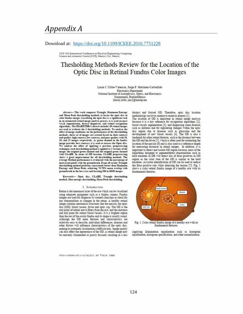
124
Appendix A
Download at: https://doi.org/10.1109/ICEEE.2016.7751228
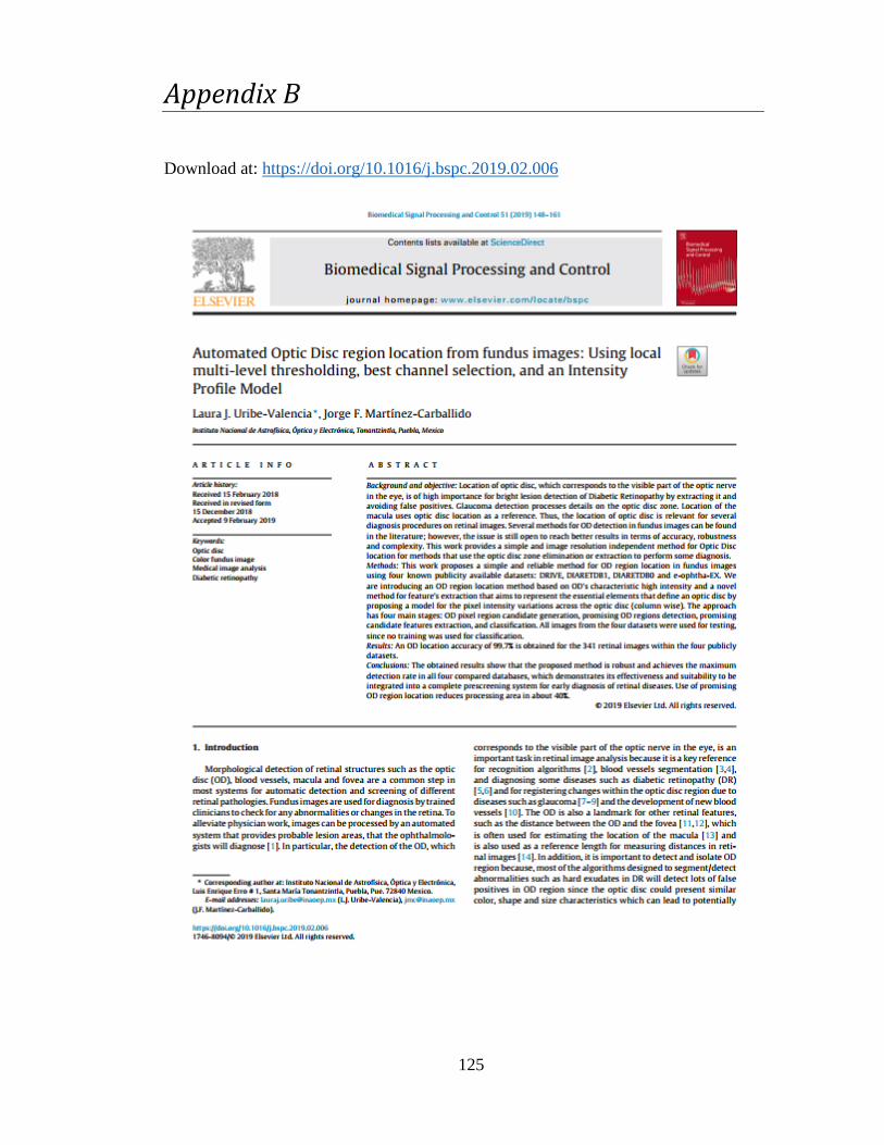
125
Appendix B
Download at: https://doi.org/10.1016/j.bspc.2019.02.006


![Neuroinflammatory responses in diabetic retinopathy...retina including the areas without clinically apparent ret-inopathy [7]. Microaneurysms, acellular capillary, and pericyte ghosts](https://img.pdfslide.net/doc/110x75/613ce6144c23507cb635ad35/neuroinflammatory-responses-in-diabetic-retinopathy-retina-including-the-areas.jpg)