Automatic elliptic grid generation by an

approximate factorisation algorithm

E. Ly∗ D. Norrison∗

30 June 2007

Abstract

A procedure for automatic numerical generation of a structured

grid system with coordinate lines coincide with all boundaries of a

general two-dimensional region containing a body of arbitrary shape

is presented. The solution procedure incorporated the method of false

transients and the approximate factorisation algorithm, where a se-

quence of time steps is cycled in a geometric fashion with repeated

endpoints, and has a capability for clustering grid lines close to the

body. The procedure requires significantly much less computational

effort to obtain a converged solution than a point or line successive

over-relaxation iterative scheme. Although, the superiority of the pre-

sented algorithm has been demonstrated for the grid generation prob-

lem, it can be utilised for other problems requiring the solution of a

set of elliptic partial differential equations of similar nature.

Contents

1 Introduction 2

2 Grid generation equations 2

3 Numerical solution procedure 3

4 Computational examples 6

5 Concluding remarks 9

∗School of Mathematical and Geospatial Sciences, SET Portfolio, RMIT University,

Melbourne, Victoria 3001, Australia. mailto:eddie.ly@rmit.edu.au

1

1 Introduction

In order to solve the governing partial differential equations (pdes) of fluiddynamics numerically, approximations to the partial differentials are intro-duced. Commonly employed numerical methods for solving the pdes requiredall partial derivatives to be converted into finite difference equations (fdes),which are solved at discrete points within the domain of interest. Therefore,a set of grid points within and on the boundaries of the domain is requiredto be specified, and so, to form a grid system. This process is known as gridgeneration [2, 8], which is the focus of the current research work.

Here we describe one of several common methods for generating smoothgrids for odd geometries, namely the elliptic grid generation method, which isused to generate a two-dimensional boundary-fitted coordinate system withquadrilateral elements. The present work is confined in two dimensions inthe interest of simplicity of the theory, but in principle, it can be extendedto three dimensions. We let the curvilinear coordinates be the solution of asystem of elliptic pdes with source terms, subjected to Dirichlet boundaryconditions on all boundaries (more details can be found in [2, 6, 8]). Thesource terms provide an option for clustering of grid line(s) or point(s), oreven a combination of both, in a specified region of the domain. One coor-dinate is specified to be constant on each of the boundaries, so that there isa coordinate line coincident with each boundary. A finite difference basedmethod, incorporating the method of false transients and the approximatefactorisation (af) algorithm [1, 3, 4, 5, 9], is employed to solve the pdes in thecomputational domain for the physical coordinates of the grid points [6, 8].In closure, grids around a body of irregular shape are generated, and con-vergence rate of the proposed numerical solution procedure will be comparedwith that of the point (psor) and line (lsor) successive over-relaxation it-erative schemes.

2 Grid generation equations

The mapping process from the physical coordinates r = (x, z) to the compu-tational coordinates ϑ = (ξ, ζ) is described by the relation ϑ = ϑ(r), whichis assumed to have continuous derivatives of all orders. In order to gener-ate an applicable grid, the mapping must be one-to-one to ensure the gridlines of the same family do not cross each other, and provides a smooth griddistribution with minimum skewness.

The following system of Poisson’s equations is considered,

ϑxx + ϑzz = S(ϑ), (1)

2

where S = (p, q) contains the source terms. As usual, ϑx and ϑxx denote∂ϑ/∂x and ∂2

ϑ/∂x2, respectively. Grid point clustering is enforced by properselection of the functions p(ϑ) and q(ϑ), and the selection is based on gridpoint or line attraction in the vicinity of defined grid line(s) or point(s), oreven a combination of both. Since it is more convenient to solve for r, whereϑ is known in the computational domain, the dependent and independentvariables of Equation (1) are interchanged to provide

(

αrξξ + Prξ

)

− 2βrξζ +(

γrζζ + Qrζ

)

= 0, (2)

where 0 is a zero vector. The constants in Equation (2) are

α = rζ · rζ , β = rξ · rζ , γ = rξ · rξ, (3)

where · represents the dot product of two vectors, and the source terms are

P =p

J2, Q =

q

J2, J =

1

xξzζ − xζzξ

, (4)

where J is the Jacobian of transformation. The solution to Equation (2) isperiodic in the ξ-direction due to the existence of a re-entrant boundary thatformed the left and right boundaries of the computational domain. Sincethe system is quasi-linear, a linearisation process must be used in the nu-merical solution procedure. For simplicity, a lagging of the coefficients (3)is employed, with the coefficients evaluated at the previous iteration or timelevel [2, 8].

3 Numerical solution procedure

Here we discuss an efficient af algorithm, together with the method of falsetransients, for solving the elliptic pde system defined by Equation (2). Anartificial time-dependent term, rτ (τ is the artificial time scale), is appendedto (2) to incorporate the temporal numerical dissipation, hence resulting in

rτ =(

αrξξ + Prξ

)

− 2βrξζ +(

γrζζ + Qrζ

)

. (5)

Since the boundary conditions are time independent for a static grid system,and provided that the numerical solution converges we anticipate that rτ

approach zero. The price paid is the loss of a true transient solution, butthis is not significant, since the objective of this work is to develop a numericalscheme that will generate the final solution at an enhanced convergence rate.

3

Table 1: Well-known time difference rules for Equation (6).

Time Difference Rule a b

Trapezoidal rule 0 1/2Euler implicit 0 1

Three-point backward 1/2 1

Euler explicit 0 0

Leap frog −1/2 0

Let τ be discretised as τ ≡ τn = n∆τ , where ∆τ is a discrete incrementof τ and n the iteration or time level, and r(τn) = r(n∆τ) = r

n. Here thespatial dependence has been temporarily suppressed. The time derivativeis approximated by a general time difference rule of a form suggested byWarming and Beam [9], which includes the rules presented in Table 1,

(

∂r

∂τ

)n

=(1 + a)

−→∆ τ − a

←−∆ τ

∆τ (1 + b−→∆ τ )

rn +

(

b− a− 1

2

)

O(∆τ) + O(∆τ)2, (6)

where−→∆ τ and

←−∆ τ are the forward and backward time difference operators.

Inserting (6) into (5) for rτ at time level τn provides(

1−∆τL)−→∆ τr

n = a←−∆ τr

n + ∆τω

bRn +

(

b−a− 1

2

)

O(∆τ)2 +O(∆τ)3, (7)

where ω is a relaxation factor,

∆τ =b ∆τ

1 + a, a =

a

1 + a, (8)

with a 6= −1, and Rn denotes the residual, which measures how well thefdes are satisfied by the approximate solution at time level τn,

Rn = Lrn =

[(

αn ∂2

∂ξ2+ P n ∂

∂ξ

)

− 2βn ∂2

∂ξ∂ζ+

(

γn ∂2

∂ζ2+ Qn ∂

∂ζ

)]

rn. (9)

In general, the operator appearing on the left side of (7) is difficult to in-vert. Therefore, in the af algorithm it is chosen as a product of two or morefactors, such that it closely resembles the operator L where only simple ma-trix operations are required, by neglecting all mixed derivatives and omittingthird- and higher-order terms in ∆τ ,

[

1−∆τ

(

αn ∂2

∂ξ2+ P n ∂

∂ξ

)][

1−∆τ

(

γn ∂2

∂ζ2+ Qn ∂

∂ζ

)]

−→∆ τr

n

= a←−∆τr

n + ∆τω

bRn. (10)

4

The factored equation (10) is then solved in an alternating direction manner,

[

1−∆τ

(

αn ∂2

∂ξ2+ P n ∂

∂ξ

)]

∆r∗ = a

←−∆ τr

n + ∆τω

bRn, (11)

[

1−∆τ

(

γn ∂2

∂ζ2+ Qn ∂

∂ζ

)]

−→∆ τr

n = ∆r∗, (12)

rn+1 = r

n +−→∆ τr

n. (13)

In each iteration, a new approximation to the solution is found by systemi-cally solving Equation (11) for the dummy temporal differences ∆r

∗, Equa-

tion (12) for the unknown vector−→∆ τr

n, and finally, applying relation (13)

to update the solution vector rn+1. When the solution converges,

−→∆τr

n ap-proach zero, and the numerical solution is given by r ≈ r

n. This methodis potentially fast since the solution process is fully vectorised, and variabletime stepping is incorporated. Note that for an accurate factorisation, and toensure that each linear system is strongly diagonally dominant, the time stepsmust be small relative to the spatial grid spacings. Ly and Gear [3, 4] ob-served that large errors can occur at the extreme ends of the frequency range,and suggested that this unfavourable behaviour be eliminated by cycling thetime steps in a geometric sense, but with repeated endpoints (∆τ1 = ∆τ2

and ∆τM−1 = ∆τM ), where M is the number of time steps per cycle.In the finite difference method, all the spatial derivatives of (11) and (12)

are discretised using standard second-order accurate central difference rules.The first spatial derivatives of coefficients (3) are discretised using standardsecond-order accurate forward, central and backward difference rules, de-pending on whether the concerned grid point is on the body boundary, aninterior grid point, or on the far-field boundary. This forms two sets of twolinear tridiagonal equation systems, instead of tridiagonal block systems ofequations as would occur if unfactored equation (7) is used. Equation (10)reduces a formidable matrix inversion problem to a series of small band-width matrix inversion problems, where efficient solution algorithms can beutilised, by reducing the two-dimensional matrix inversion problem to twoone-dimensional problems. Equation (11) forms a so-called cyclic tridiagonalsystem (due to the periodic boundary conditions at the re-entrant boundary),which is inverted by applying the Sherman-Morrison formula [7] togetherwith a standard tridiagonal system solver, treating the system as tridiagonalplus a small correction. While Equation (12) forms a pure tridiagonal sys-tem that can be efficiently inverted by any robust tridiagonal solver. Whena 6= 0, Equations (11) and (12) form a three time level iterative scheme,which requires no additional computation and no additional storage as com-

5

Table 2: Comparison of computational times.

Algorithm psor lsor af1 af2

Iterations 189 603 31 37

Error, E 4.980(

10−5)

4.975(

10−5)

4.981(

10−5)

4.988(

10−5)

Total cpu time 0.291 secs 1.963 secs 0.181 secs 0.271 secs

Iteration

Err

or

0 100 200 300 400 500 600 70010-5

10-4

10-3

10-2

PSORLSOR

AF2(red)

AF1

Africa

ωPSOR = 1.900

ωLSOR = 1.046

ωAF1 = 2.014

ωAF2 = 1.713

Iteration

Max

imum

Res

idua

l

0 5 10 15 20 25 30 35 4010-7

10-6

10-5

10-4

10-3

10-2 Africa

AF1

AF2

∆τmin = 100

∆τmax = 20, 000

M = 6 (rep)

Figure 1: Convergence histories.

pared to the two time level scheme (when a = 0) that requires two levels

of data, namely rn and

−→∆ τr

n. At the start of an iteration, rn and

←−∆τr

n

are both known subsequent to advancing the solution from time level τn toτn+1 using (11) to (13). After ∆r

∗ has been computed from (11) along a

ζ-constant line,←−∆ τr

n along this same line is no longer required, and is over

written with the ∆r∗ values. Similarly, as

−→∆τr

n is computed from (12) alonga ξ-constant line, the new result is written in the storage space containingthe ∆r

∗ values.

4 Computational examples

The af algorithm is employed with an Euler implicit time difference rule(a = 0, b = 1) to generate an O-type grid system around a body of irregularshape represented by the continent Africa, with 87 points around the bodycontour and 31 points in the radial direction. It was found, through numericalexperiments, that the af algorithm became unstable if the Euler explicitand leap frog time difference rules were used. A cycle of six time steps

6

X

Z

-2 0 2 4-4

-2

0

2

4

Initial grid X

Z

-2 0 2 4-4

-2

0

2

4

After 10th iteration

X

Z

-2 0 2 4-4

-2

0

2

4

After 22nd iteration X

Z

-2 0 2 4-4

-2

0

2

4

Final grid

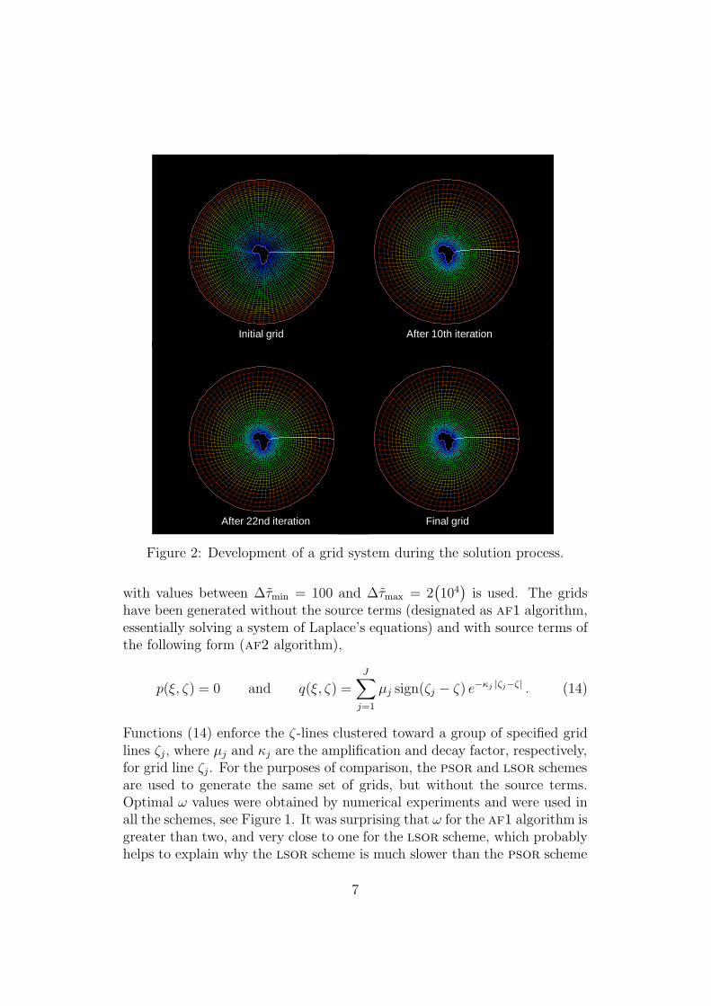
Figure 2: Development of a grid system during the solution process.

with values between ∆τmin = 100 and ∆τmax = 2(

104)

is used. The gridshave been generated without the source terms (designated as af1 algorithm,essentially solving a system of Laplace’s equations) and with source terms ofthe following form (af2 algorithm),

p(ξ, ζ) = 0 and q(ξ, ζ) =

J∑

j=1

µj sign(ζj − ζ) e−κj |ζj−ζ| . (14)

Functions (14) enforce the ζ-lines clustered toward a group of specified gridlines ζj, where µj and κj are the amplification and decay factor, respectively,for grid line ζj. For the purposes of comparison, the psor and lsor schemesare used to generate the same set of grids, but without the source terms.Optimal ω values were obtained by numerical experiments and were used inall the schemes, see Figure 1. It was surprising that ω for the af1 algorithm isgreater than two, and very close to one for the lsor scheme, which probablyhelps to explain why the lsor scheme is much slower than the psor scheme

7

X

Z

-2 0 2 4-4

-2

0

2

4

Without source terms X

Z

-2 0 2 4-4

-2

0

2

4

With source terms

X

Z

-1 0 1 2

-1

0

1

X

Z

-1 0 1 2

-1

0

1

Figure 3: Generating grid systems without (left plots) and with (right plots)grid lines clustering towards ζ1- to ζ4-line with µ = (100, 100, 90, 90) andκ = (0.2, 0.2, 0.25, 0.3).

in reaching convergence (see Table 2). All schemes are terminated when theerror (representing the total changes in the solution) per grid point, E, is lessthan 5

(

10−5)

. Figure 1 compares the convergence history of all schemes, andshows that the maximum residual of the af algorithms reduce substantiallywhenever the algorithms completed one cycle of time steps. Overall, theerrors decrease in a logarithmical manner, and the af algorithms require theleast number of iterations for convergence.

Since a single af iteration requires more computational (cpu) time thana single psor or lsor iteration, a comparison of the number of iterationsrequired for convergence is not meaningful. Therefore, the actual CPU timesrequired for convergence on an ibm ThinkPad t22 model notebook withan Intel Pentinum iii processor of speed 995 MHz, running the MicrosoftWindows xp Professional operating system with 384mb of physical memoryand 576mb of virtual memory are compared in Table 2. The comparisons

8

show that the af1 algorithm is about twice faster than the psor scheme, andten times faster than the lsor scheme. The authors observed that the speedat which the scheme converges mainly depended on the manner in which theshape of the branch-cuts are changing from one iteration to the next. In theaf algorithm, the grid points along the branch-cut are included implicitlyinto the equation system, and so, the branch-cut points are updated withall other interior points simultaneously (as illustrated in Figure 2). Whilefor the psor and lsor schemes, these grid points are computed after eachiteration, hence the branch-cuts are updated with one iteration level lapsed.When the source terms are included, the number of iterations required forconvergence by the af2 algorithm increases by 20 %, and the computationaltime increases by 50 %.

Careful examination of the plots in Figure 2 (where the grids shown afterthe 10th, 22nd and final iterations are visually indistinguishable), and Figure 3clearly indicate a smooth distribution of the grid points within the domain,in particular noting the adjustment of the grid points on the branch-cut. Thenatural clustering of grid points due to the elliptic nature of the governingpdes, and enforced clustering of grid lines due to the inclusion of the sourceterms toward the body can be seen. The final grid is correctly generated, eventhough the initial grid is badly distorted with grid lines crossing and highlyskewed in some regions near the body, which makes the process suitable forautomatic grid generation computer code.

5 Concluding remarks

A system of Poisson’s equations is solved in the computational domain by afinite difference method to generate a structured grid around a single bodyof arbitrary shape in two dimensions. In the af algorithm, the method offalse transients is incorporated, in which a sequence of time steps is cycled ina geometric fashion with repeated endpoints. It was found that the proposedaf algorithm (with and without the source terms for clustering of grid linestowards the body) is significantly faster in reaching convergence to the user’srequired accuracy than both the psor and lsor schemes. It was observedthat if the employed numerical scheme is numerically stable and converged,a correct final grid system can always be obtained independent of the formof its initial grid system, and hence, make it suitable for automatic gridgeneration computer code. No restrictions are enforced on the shape of theboundaries, which may even be time dependent, and the approach can beextended to generating grids for body of arbitrary shapes in three dimensions.Although, the superiority of the af algorithm has been demonstrated for the

9

automatical grid generation problem, it can be utilised for other problemsrequiring the solution of a set of elliptic pdes of similar nature.

References

[1] Catherall, D., Optimum Approximate-Factorization Schemes for Two-Dimensional Steady Potential Flows, AIAA Journal, 20, 8, 1982, pp.1057–1063.

[2] Hoffmann, K. A., Computational Fluid Dynamics for Engineers, Engi-neering Educational System, Texas, USA, 1989.

[3] Ly, E., Improved Approximate Factorisation Algorithm for the SteadySubsonic and Transonic Flow over an Aircraft Wing, in Proceedings of the21st Congress of the International Council of the Aeronautical Sciences(ICAS98), AIAA & ICAS, Melbourne, Australia, Sep. 1998, Paper A98-31699.

[4] Ly, E., and Gear, J. A., Time-Linearized Transonic Computations Includ-ing Shock Wave Motion Effects, Journal of Aircraft, 39, 6, Nov./Dec.2002, pp. 964–972.

[5] Ly, E., and Nakamichi, J., Time-Linearised Transonic Computations In-cluding Entropy, Vorticity and Shock Wave Motion Effects, The Aero-nautical Journal, Nov. 2003, pp. 687–695.

[6] Mathur, J. S., and Chakrabartty, S. K., An Approximate FactorizationScheme for Elliptic Grid Generation with Control Functions, NumericalMethods for Partial Differential Equations, 10, 6, 1994, pp. 703–713.

[7] Press, W. H., Teukolsky, S. A., Vetterling, W. T., and Flannery, B. P.,Numerical Recipes in FORTRAN: The Art of Scientific Computing, Sec-ond Edition, Cambridge University Press, USA, 1994.

[8] Thompson, J. F., Thames, F. C., and Mastin, C. W., Boundary-FittedCurvilinear Coordinate Systems for Solution of Partial Differential Equa-tions on Fields Containing any Number of Arbitrary Two-DimensionalBodies, NASA Contractor Report CR-2729, Washington DC, USA, July1977, 253 pages.

[9] Warming, R. F., and Beam, R. M., On the Construction and Applica-tion of Implicit Factored Schemes for Conservation Laws, in SIAM-AMSProceedings, 11, USA, 1978, pp. 85–129.

10