ISSN 0103-9741

Monografias em Ciência da Computação

n° 04/09

Automatic Embryonic Stem Cells Detection and Counting Method in Fluorescence

Microscopy Images

Geisa Martins Faustino Marcelo Gattass

Paulo Cezar Pinto Carvalho Stevens Rehen

Carlos José Pereira de Lucena

Departamento de Informática

PONTIFÍCIA UNIVERSIDADE CATÓLICA DO RIO DE JANEIRO

RUA MARQUÊS DE SÃO VICENTE, 225 - CEP 22451-900

RIO DE JANEIRO - BRASIL

Monografias em Ciência da Computação, No. 04/09 ISSN: 0103-9741Editor: Prof. Carlos José Pereira de Lucena February, 2009

Automatic Embryonic Stem Cells Detection and Countingin Fluorescence Microscopy Images

Geisa Martins Faustino, Marcelo Gattass, Paulo Cezar Pinto Carvalho, Stevens Rehen andCarlos José Pereira de Lucena

gfaustino@inf.puc-rio.br, mgattass@tecgraf.puc-rio.br, pcezar@impa.br, srehen@anato.ufrj.br,lucena@les.puc-rio.br

Abstract. In this paper, we propose an automatic embryonic stem cell detection and countingmethod in fluorescence microscopy images. We handle with pluripotent stem cells cultured invitro. Our approach uses the luminance information to generate a graph-based image representa-tion. Then, a graph mining process is used to detect the cells. The proposed method was exten-sively tested on a database of 92 images and the results were validated by specialists. We obtainedan average precision, recall and F-measure of 93.97%, 92.04% and 92.87%, respectively.

Keywords: Automated cell counting, fluorescence microscopy images, graph based image repre-sentation, graph mining.

Resumo. Neste artigo, nós propomos um método automático para detecção e contagem de célulastronco embrionárias em imagens de micrsocopia fluorescente. Nós lidamos com células troncocultivadas in vitro. Nossa abordagem utiliza a informação de luminância para gerar uma represen-tacão da imagem baseada em grafo. Então, um processo de mineração é utilizado para detectaras células. O método proposto foi exaustivamente testado numa base de dados composta por 92imagens e os resultaos foram revisados por especialistas. Nós obtivemos uma precision, recall eF-measure média de 93.97%, 92.04% and 92.87%, respectivamente.

Palavras-chave: Contagem automática de células, imagens de micrsocopia fluorescente, repre-sentacão de imagem baseada em grafo, mineração de grafo.

In charge of publications:Rosane Teles Lins CastilhoAssessoria de Biblioteca, Documentação e InformaçãoPUC-Rio Departamento de InformáticaRua Marquês de São Vicente, 225 - Gávea22451-900 Rio de Janeiro RJ BrasilTel. +55 21 3527-1516 Fax: +55 21 3527-1530E-mail: bib-di@inf.puc-rio.brWeb site: http://bib-di.inf.puc-rio.br/techreports/

1 Introduction

Embryonic stem cells are self-renewing elements that, through mitotic cell division and differen-tiation process, can generate all three germ layers (endoderm, ectoderm and mesoderm) and alsospecialized adult cells such as neurons, osteoblasts, cardiomyocytes, hepatocytes of the humanbody. They are found in various parts of the human body at every stage of development fromembryo to adult and are classified according to their potential to develop into other cell types. Apleuripotent stem cell can develop into cells from all three germinal layers while multipotent stemcells can generate only closely related family of cells (e.g. hematopoietic stem cells differentiateinto red blood cells, white blood cells, platelets, etc.). These characteristics of pluripotency makethem a promising alternative for cell-based treatments of various diseases. Their differentiationprocess can be recapitulated by culturing those cells in non-adherent plates when cystic structurescharacterized by cavitations and fluid accumulation called embryoid bodies are formed.

Using different cell markers, specialists are able to determine, by manual counting, the totalnumber of cells, how many specialized itself into a specific mature cell and how many cells died.These statistics are used to understand and validate the experiments. However, given the absence ofhigh contrast, large number of cluttered objects in a single scene, occlusion, tuning in microscopyparameters and variability of cell size and morphology, detect and count these cells is a difficulttask. Moreover, it requires a high level of concentration that makes manual screening a tediousand time-consuming task. In addition, the results are subjective and can greatly variate accordingto the personal interpretation of each specialist. Therefore, there is a strong motivation for thedevelopment of an automatic cell detection and counting method, which can be a useful tool forunderstanding and accelerating the stem cell therapy process.

There are methods [28, 21] to identify and quantify sections of cells cultured in suspension.However, these methods are expensive and require a trained technical specialist. Another disad-vantage is that the spatial information is lost, because the cells must be separated. This informationis important because the specialists are able to observe some phenomena, such as, the differenti-ated cells are located in the colony’s extremity while the specialized stem cells are located at thecolony’s center [9].

Several researchers have been developing automated methods for segmenting and countingcells in microscopy images [29, 31, 5, 36, 11, 30, 4]. Some approaches are based on machinelearning [22, 23, 34]. Long et al. [22] and Zheng et al. [34] proposed methods based on neuralnetwork and Markiewicz et al. [23] proposed a method to cell recognition and count using SupportVector Machine. In this kind of approach, the major task is to create the learning set, which isusually done manually by an independent expert for cell type. Another disadvantage is the timespend on training and parameter adjust. Approaches that use classical segmentation methods, suchas threshold, morphological filtering and watershed transformation [3, 26, 12, 7] also have beenproposed. With the discovery of the stem cells potential, many researches have been dealing withthis kind of cell [24, 8, 18, 19, 2, 32, 15, 17, 16, 20]. Althoff et al. [2] and Tang et al. [32] proposeda method for segmentation and tracking of neural stem cells (NSC). Both approaches are basedon classical segmentation methods and use the information about the cells’ previous position todecide which blobs correspond to real cells. Also working with NSC, Korzynska [20] presented amethod for automatic counting of neural stem cells growing in cultures which is performed in twosteps: 1) segmentation step: the image is separated in several regions and; 2)counting step: eachhomogeneous region is counted separately. Some approaches handle with hematopoietic stemcells (HSC) [15, 17, 16]. Kachouie et al. [15] proposed a deconvolution method in the form of anoptimized ellipse fitting algorithm to locate individuals HSC. The methods proposed in [17, 16],

4

uses the cell morphologic information (e. g. cell size, boundary brightness, interior brightnessand boundary uniformity or symmetry) to locate and track HSC. Note that, the works cited abovehandled with only one type of stem cell in their images.

In this paper, we propose an automatic method for detecting and counting stem cells sectionsobtained under in fluorescence microscopy. We handle with embryoid bodies obtained from em-bryonic stem cells cultured in vitro. Our approach uses the luminance information to generate agraph-based image representation. Each cell is represented in the graph as a particular structurethat we called simple path. Then, a graph mining process is used to detect the cells. While our mo-tivation is to count stem cells, our approach can also be applied in other groups of objects, as longas the object surface are both smooth and concave with only one punctual illumination source. Theproposed method was extensively tested on a database of 92 images and the results were validatedby specialists. We obtained, in average, a precision, recall and F-measure of 93.97%, 92.04% and92.87% respectively. We also have tested the proposed approach in others objects, such as seeds,candies and spots in electrophoresis images [13, 14]. Although counting cells are a well knowproblem, we are not aware of any other work that handles with several types of pluripotent stemcells in the same image.

The remainder of this paper is organized as follows: section 2 details the image characteristics;section 3 describes the proposed method; section 4 presents the experimental results to show theeffectiveness of the method and; section 5 presents our conclusion and some future works.

2 Image Characterization

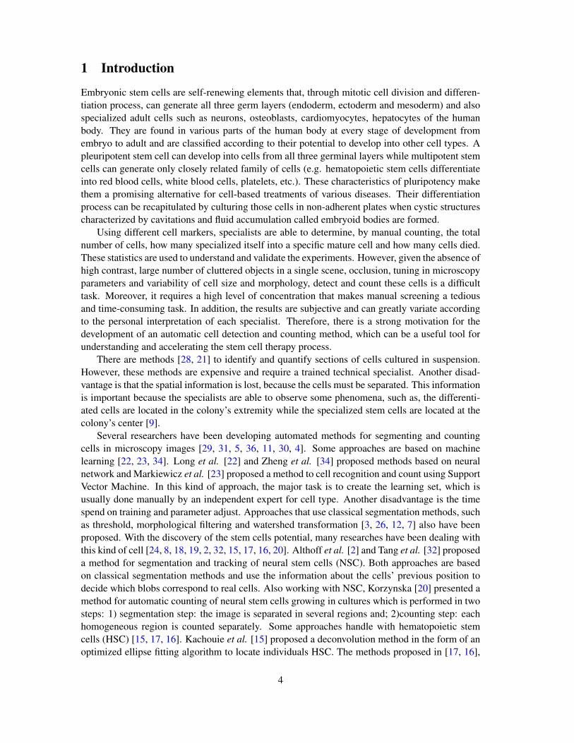
The images of embryoid bodies used in this work were collected in the Institute of BiomedicalSciences at UFRJ/Brazil. Shortly, embryoid bodies were cultured for 8 days under a neural dif-ferentiation process. In this procedure the embryoid bodies were stimulated to differentiate intoa neural phenotype by the incubation, on the last 4 days, with retinoic acid at final concentrationof 2µM . After this time, they were fixed in 4% parafolmaldehyde (PF) solution for 30 minutes,passed through a sucrose gradient (10, 20 and 30%, 30 minutes each) and finally embeeded intissue tek R© OCT (optimum compound temperature) for cryopreserving. Slices were prepared oncryostat to discern the number of individual cells on each embryoid body. The slice thicknessused was 10µm, which corresponds to the nuclei average size. Next, the slices were incubated, for5 minutes, with 4‘-6-Diamidino-2-phenylindole (DAPI), which is a kind of nuclei counter stain.The acquisition system consists of a Nikon Eclipse TE300 inverted epi-fluoresence microscope, aMagnaFire Digital CCD camera and the Image Pro Express software. The procedure of acquisi-tion is semi-automatic and the specialist controls some parameters, such as, magnification, timeexposure and focus. The resolution of the captured images were 1032× 1040 pixels, which corre-spond to zoom of 40×. They were stored using Tagged Image File (.tif) format with lossless LZWcompression. Figure 1 shows an example of a captured image.

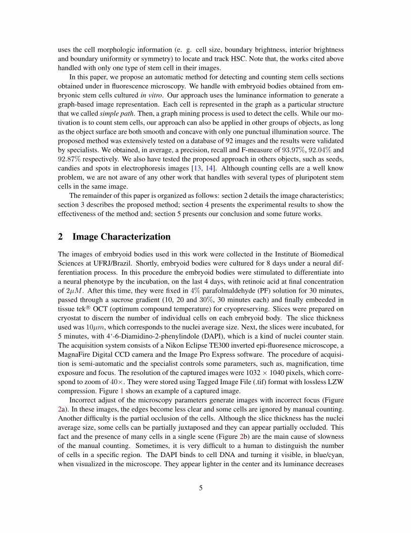
Incorrect adjust of the microscopy parameters generate images with incorrect focus (Figure2a). In these images, the edges become less clear and some cells are ignored by manual counting.Another difficulty is the partial occlusion of the cells. Although the slice thickness has the nucleiaverage size, some cells can be partially juxtaposed and they can appear partially occluded. Thisfact and the presence of many cells in a single scene (Figure 2b) are the main cause of slownessof the manual counting. Sometimes, it is very difficult to a human to distinguish the numberof cells in a specific region. The DAPI binds to cell DNA and turning it visible, in blue/cyan,when visualized in the microscope. They appear lighter in the center and its luminance decreases

5

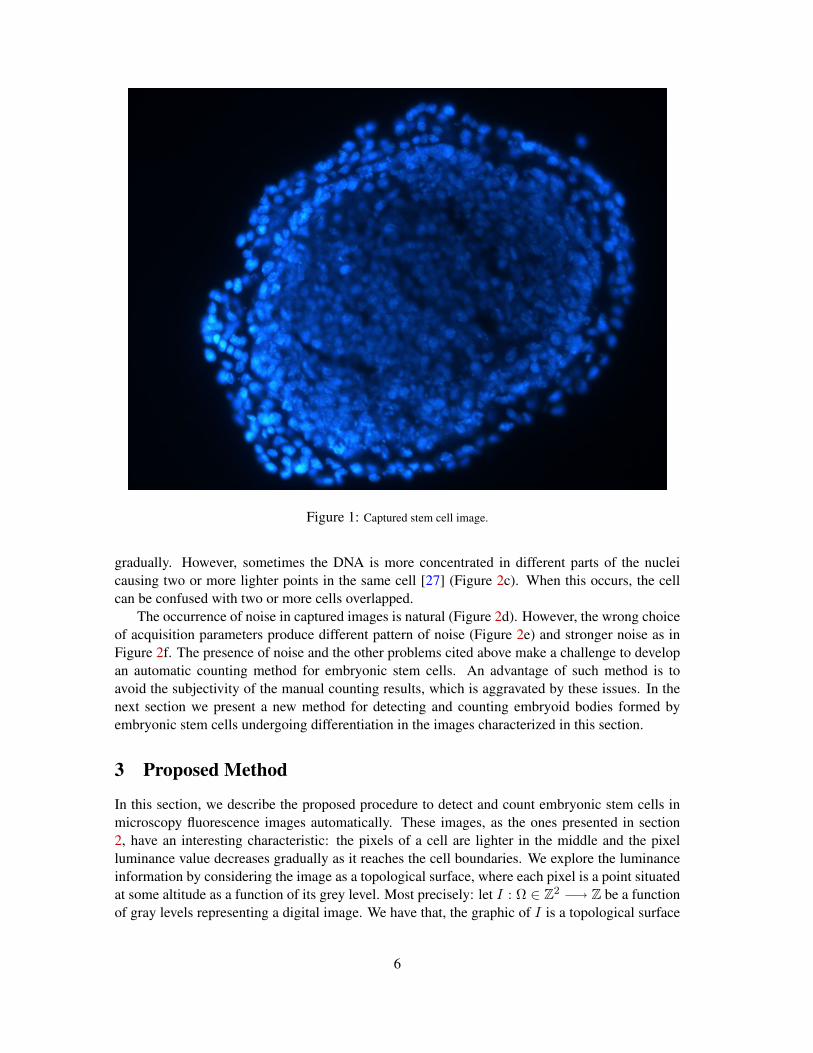
Figure 1: Captured stem cell image.

gradually. However, sometimes the DNA is more concentrated in different parts of the nucleicausing two or more lighter points in the same cell [27] (Figure 2c). When this occurs, the cellcan be confused with two or more cells overlapped.

The occurrence of noise in captured images is natural (Figure 2d). However, the wrong choiceof acquisition parameters produce different pattern of noise (Figure 2e) and stronger noise as inFigure 2f. The presence of noise and the other problems cited above make a challenge to developan automatic counting method for embryonic stem cells. An advantage of such method is toavoid the subjectivity of the manual counting results, which is aggravated by these issues. In thenext section we present a new method for detecting and counting embryoid bodies formed byembryonic stem cells undergoing differentiation in the images characterized in this section.

3 Proposed Method

In this section, we describe the proposed procedure to detect and count embryonic stem cells inmicroscopy fluorescence images automatically. These images, as the ones presented in section2, have an interesting characteristic: the pixels of a cell are lighter in the middle and the pixelluminance value decreases gradually as it reaches the cell boundaries. We explore the luminanceinformation by considering the image as a topological surface, where each pixel is a point situatedat some altitude as a function of its grey level. Most precisely: let I : Ω ∈ Z2 −→ Z be a functionof gray levels representing a digital image. We have that, the graphic of I is a topological surface

6

(a) (b) (c)

(d) (e) (f)

Figure 2: Image features: a) image out of focus; b) partial occlusion and many objects in a sin-gle scene; c) the DNA condensation phenomena [27] (the black arrows point out the two lighterpoints); d) presence of acceptable level of noise; e) presence of weak noise and; f)presence ofstrong noise.

in which the altitude of every point is equal to the gray level of the corresponding pixel (see Figure3). Moreover, we have that each cell can be identified as a set of local maximum points, becausethe presence of noise and the DNA condensation phenomena. Therefore, the classical methods[25, 6] cannot be applied directly. The method proposed in [6] generate an over segmentation andmany artifacts are classified, wrongly, as cell. The method proposed in [25], uses a neighborhoodof fix size and all pixels whose intensity is not maximal within this neighborhood are ignored.Thus, if there are more than one cell in this region, only one are counted. On the other hand, if theregion size is too small many artifacts are classified, wrongly, as cell.

(a) (b) (c)

Figure 3: Surface plot: a) input image; b) surface plot and c) surface plot after a Gaussian blurfilter. Note that in b), due to presence of noise and the DNA condensation phenomena, one cell isrepresented by a set of maximum point. However, after the Gaussian filter, because it smoothedthe surface and emphasize the maximum points, many cells are represented by only one localmaximum point.

We detected local maximum points tracing level curves in which the set of points (x, y) ∈ Ωthat satisfies c ≤ I(x, y) < c + ε, where c, ε ∈ Z+, corresponds to the image pixels that belongs

7

to the level c. Likewise, this can be done parting the histogram image as described below. Forthis images, the green channel supply more information than the gray scale image. Thus, ourluminance information is based on this channel.

Our method has four main steps: 1) pre-processing; 2) histogram partition and connectedcomponent detection; 3) graph construction; and 4) graph mining process, which we shall discussin the sequel.

3.1 Preprocessing

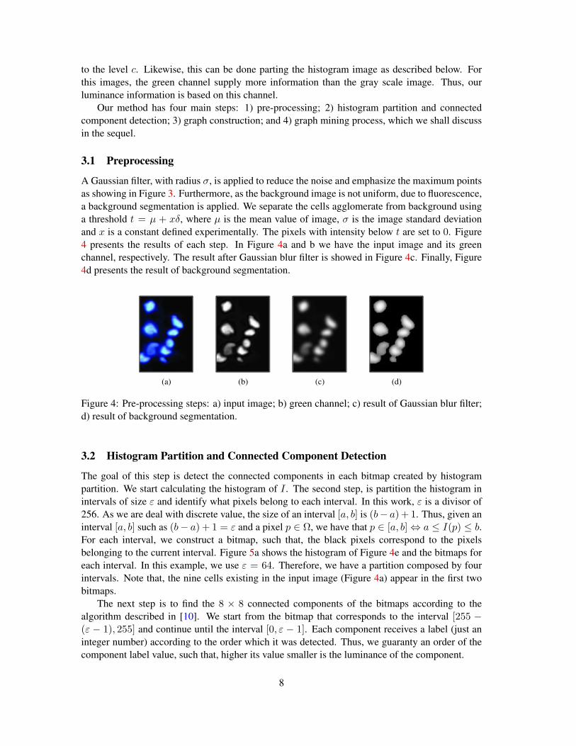
A Gaussian filter, with radius σ, is applied to reduce the noise and emphasize the maximum pointsas showing in Figure 3. Furthermore, as the background image is not uniform, due to fluorescence,a background segmentation is applied. We separate the cells agglomerate from background usinga threshold t = µ + xδ, where µ is the mean value of image, σ is the image standard deviationand x is a constant defined experimentally. The pixels with intensity below t are set to 0. Figure4 presents the results of each step. In Figure 4a and b we have the input image and its greenchannel, respectively. The result after Gaussian blur filter is showed in Figure 4c. Finally, Figure4d presents the result of background segmentation.

(a) (b) (c) (d)

Figure 4: Pre-processing steps: a) input image; b) green channel; c) result of Gaussian blur filter;d) result of background segmentation.

3.2 Histogram Partition and Connected Component Detection

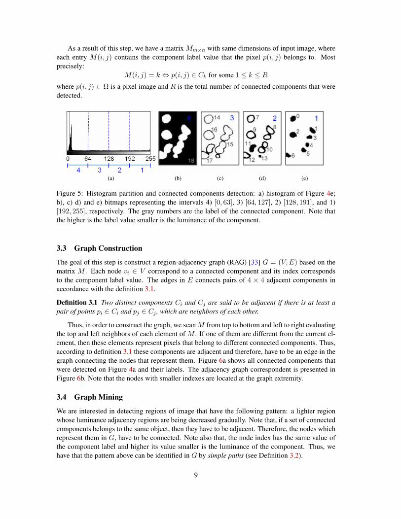
The goal of this step is detect the connected components in each bitmap created by histogrampartition. We start calculating the histogram of I . The second step, is partition the histogram inintervals of size ε and identify what pixels belong to each interval. In this work, ε is a divisor of256. As we are deal with discrete value, the size of an interval [a, b] is (b− a) + 1. Thus, given aninterval [a, b] such as (b− a) + 1 = ε and a pixel p ∈ Ω, we have that p ∈ [a, b]⇔ a ≤ I(p) ≤ b.For each interval, we construct a bitmap, such that, the black pixels correspond to the pixelsbelonging to the current interval. Figure 5a shows the histogram of Figure 4e and the bitmaps foreach interval. In this example, we use ε = 64. Therefore, we have a partition composed by fourintervals. Note that, the nine cells existing in the input image (Figure 4a) appear in the first twobitmaps.

The next step is to find the 8 × 8 connected components of the bitmaps according to thealgorithm described in [10]. We start from the bitmap that corresponds to the interval [255 −(ε − 1), 255] and continue until the interval [0, ε − 1]. Each component receives a label (just aninteger number) according to the order which it was detected. Thus, we guaranty an order of thecomponent label value, such that, higher its value smaller is the luminance of the component.

8

As a result of this step, we have a matrix Mm×n with same dimensions of input image, whereeach entry M(i, j) contains the component label value that the pixel p(i, j) belongs to. Mostprecisely:

M(i, j) = k ⇔ p(i, j) ∈ Ck for some 1 ≤ k ≤ Rwhere p(i, j) ∈ Ω is a pixel image and R is the total number of connected components that weredetected.

(a) (b) (c) (d) (e)

Figure 5: Histogram partition and connected components detection: a) histogram of Figure 4e;b), c) d) and e) bitmaps representing the intervals 4) [0, 63], 3) [64, 127], 2) [128, 191], and 1)[192, 255], respectively. The gray numbers are the label of the connected component. Note thatthe higher is the label value smaller is the luminance of the component.

3.3 Graph Construction

The goal of this step is construct a region-adjacency graph (RAG) [33] G = (V,E) based on thematrix M . Each node vi ∈ V correspond to a connected component and its index correspondsto the component label value. The edges in E connects pairs of 4 × 4 adjacent components inaccordance with the definition 3.1.

Definition 3.1 Two distinct components Ci and Cj are said to be adjacent if there is at least apair of points pi ∈ Ci and pj ∈ Cj , which are neighbors of each other.

Thus, in order to construct the graph, we scanM from top to bottom and left to right evaluatingthe top and left neighbors of each element of M . If one of them are different from the current el-ement, then these elements represent pixels that belong to different connected components. Thus,according to definition 3.1 these components are adjacent and therefore, have to be an edge in thegraph connecting the nodes that represent them. Figure 6a shows all connected components thatwere detected on Figure 4a and their labels. The adjacency graph correspondent is presented inFigure 6b. Note that the nodes with smaller indexes are located at the graph extremity.

3.4 Graph Mining

We are interested in detecting regions of image that have the following pattern: a lighter regionwhose luminance adjacency regions are being decreased gradually. Note that, if a set of connectedcomponents belongs to the same object, then they have to be adjacent. Therefore, the nodes whichrepresent them in G, have to be connected. Note also that, the node index has the same value ofthe component label and higher its value smaller is the luminance of the component. Thus, wehave that the pattern above can be identified in G by simple paths (see Definition 3.2).

9

Definition 3.2 A simple path in a graph G = (V,E) can be defined as a subgraph S that satisfy:

i) the nodes in S are connected to other nodes in S;

ii) each node of S has a maximum degree of two and;

iii) the index value of a node is smaller than the one of its adjacent node and bigger than the oneof other adjacent node, if it exists (i.e. the index values of the nodes in S are in increasingorder).

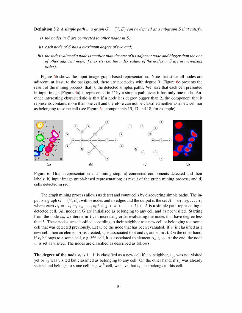
Figure 6b shows the input image graph-based representation. Note that since all nodes areadjacent, at least, to the background, there are not nodes with degree 0. Figure 6c presents theresult of the mining process, that is, the detected simples paths. We have that each cell presentedin input image (Figure 4a) is represented in G by a simple path, even it has only one node. An-other interesting characteristic is that if a node has degree bigger than 2, the component that itrepresents contains more than one cell and therefore can not be classified neither as a new cell noras belonging to some cell (see Figure 6a, components 15, 17 and 18, for example).

(a) (b) (c) (d)

Figure 6: Graph representation and mining step: a) connected components detected and theirlabels; b) input image graph-based representation; c) result of the graph mining process; and d)cells detected in red.

The graph mining process allows us detect and count cells by discovering simple paths. The in-put is a graphG = (V,E), with n nodes andm edges and the output is the setA = α1, α2, . . . , αk

where each αi = vi, vj , vk, . . . , vl|i < j < k < · · · < l ∈ A is a simple path representing adetected cell. All nodes in G are initialized as belonging to any cell and as not visited. Startingfrom the node v0, we iterate in V , in increasing order evaluating the nodes that have degree lessthan 3. These nodes, are classified according to their neighbor as a new cell or belonging to a somecell that was detected previously. Let vi be the node that has been evaluated. If vi is classified as anew cell, then an element αi is created, vi is associated to it and αi added in A. On the other hand,if vi belongs to a some cell, e.g. kth cell, it is associated to element αk ∈ A. At the end, the nodevi is set as visited. The nodes are classified as described as follows:

The degree of the node vi is 1 It is classified as a new cell if: its neighbor, vj , was not visitedyet or vj was visited but classified as belonging to any cell. On the other hand, if vj was alreadyvisited and belongs to some cell, e.g. kth cell, we have that vi also belongs to this cell.

10

The degree of the node vi is 2 Let vj and vk be its neighbors. We have six possibilities: 1) vj

and vk was already visited and both was classified as belonging to the same cell, e.g. mth cell; 2)vj and vk was visited and classified as belonging to any cell; 3) vj and vk was visited and classifiedas belonging to different cells; 4) one of them, e.g. vj , was visited and classified as belonging tosome cell e.g. mth cell, and the other, vk, was not visited yet; 5) one of them, e.g. vj , was visitedand classified as belonging to some cell e.g. mth cell, and the other, vk was visited and classifiedas belongs to any cell; and 6) vj and vk was not visited yet. If 1), 4) or 5) occur, vi is classified asbelonging to the mth cell. If 2) or 3) occur, we can not associate vi to any element of A becausewe find out a component that contains more than one cell. If 6) occur, as we are going through Vin increasing order, we find a new cell.

4 Experimental Results

In this section, we evaluate the proposed method and analyze the experimental results. The pro-posed method was implemented in Java language 6.0 using the development tool Eclipse 3.2. Thetests were executed on an Intel Core 2 Duo CPU T7500 2.20GHz with 2Gb RAM.

A database with 92 images of stem cells was constructed and divided in two groups: group1, with 69 images with an acceptable level of noise and; group 2 formed by 23 images withthe presence of strong noise. Additional experiments were performed for a third image groupcomposed by 5 images of seeds, candies and spots in electrophoresis images [13]. The valuesfor the input parameters σ, x and ε of the preprocessing step were obtained through experimentaltests. The value for the Gaussian radius σ were 2,3 and 3 for the groups 1, 2 and 3, respectively.The threshold t were calculated using x = 0.3 for all groups. The histogram were partitioned inintervals of size ε = 8 for the groups 1 and 2. For the third group, the value of ε was chosenamong 8, 16 and 32 that best fitted each image.

Specialists from Institute of Biomedical Sciences – UFRJ/Brazil validated the experimentalresults obtained by the proposed method. They pointed out cells that were not counted and artifactsthat were incorrectly classified as cells. The results are evaluated by calculating the measuresprecision, recall and F-measure as shown as follow:

Precision =tp

tp+ fp(1)

Recall =tp

tp+ fn(2)

F −measure =2 ∗ Precision ∗RecallPrecision+Recall

(3)

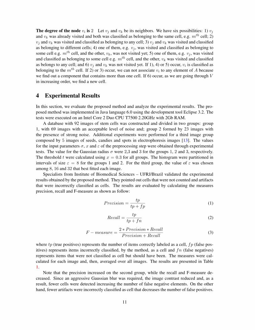
where tp (true positives) represents the number of items correctly labeled as a cell, fp (false pos-itives) represents items incorrectly classified, by the method, as a cell and fn (false negatives)represents items that were not classified as cell but should have been. The measures were cal-culated for each image and, then, averaged over all images. The results are presented in Table1.

Note that the precision increased on the second group, while the recall and F-measure de-creased. Since an aggressive Gaussian blur was required, the image contrast reduced and, as aresult, fewer cells were detected increasing the number of false negative elements. On the otherhand, fewer artifacts were incorrectly classified as cell that decreases the number of false positives.

11

Precision Recall F-measure(%) (%) (%)

Group 1 93.84 92.67 93.12Group 2 94.32 90.33 92.18

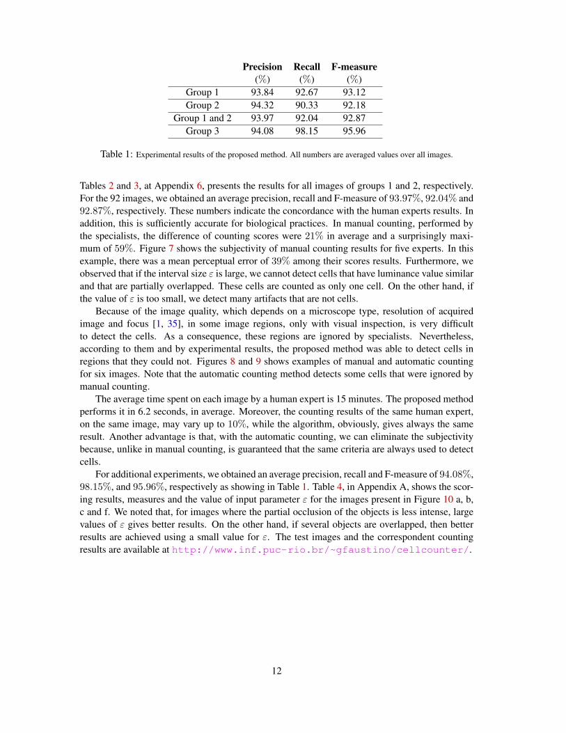
Group 1 and 2 93.97 92.04 92.87Group 3 94.08 98.15 95.96

Table 1: Experimental results of the proposed method. All numbers are averaged values over all images.

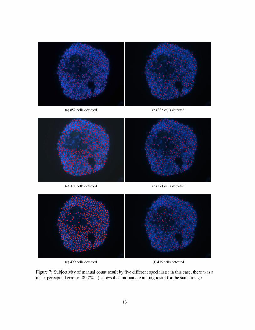
Tables 2 and 3, at Appendix 6, presents the results for all images of groups 1 and 2, respectively.For the 92 images, we obtained an average precision, recall and F-measure of 93.97%, 92.04% and92.87%, respectively. These numbers indicate the concordance with the human experts results. Inaddition, this is sufficiently accurate for biological practices. In manual counting, performed bythe specialists, the difference of counting scores were 21% in average and a surprisingly maxi-mum of 59%. Figure 7 shows the subjectivity of manual counting results for five experts. In thisexample, there was a mean perceptual error of 39% among their scores results. Furthermore, weobserved that if the interval size ε is large, we cannot detect cells that have luminance value similarand that are partially overlapped. These cells are counted as only one cell. On the other hand, ifthe value of ε is too small, we detect many artifacts that are not cells.

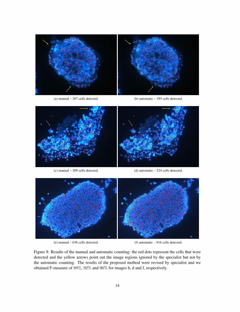
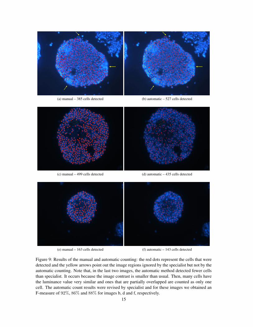
Because of the image quality, which depends on a microscope type, resolution of acquiredimage and focus [1, 35], in some image regions, only with visual inspection, is very difficultto detect the cells. As a consequence, these regions are ignored by specialists. Nevertheless,according to them and by experimental results, the proposed method was able to detect cells inregions that they could not. Figures 8 and 9 shows examples of manual and automatic countingfor six images. Note that the automatic counting method detects some cells that were ignored bymanual counting.

The average time spent on each image by a human expert is 15 minutes. The proposed methodperforms it in 6.2 seconds, in average. Moreover, the counting results of the same human expert,on the same image, may vary up to 10%, while the algorithm, obviously, gives always the sameresult. Another advantage is that, with the automatic counting, we can eliminate the subjectivitybecause, unlike in manual counting, is guaranteed that the same criteria are always used to detectcells.

For additional experiments, we obtained an average precision, recall and F-measure of 94.08%,98.15%, and 95.96%, respectively as showing in Table 1. Table 4, in Appendix A, shows the scor-ing results, measures and the value of input parameter ε for the images present in Figure 10 a, b,c and f. We noted that, for images where the partial occlusion of the objects is less intense, largevalues of ε gives better results. On the other hand, if several objects are overlapped, then betterresults are achieved using a small value for ε. The test images and the correspondent countingresults are available at http://www.inf.puc-rio.br/~gfaustino/cellcounter/.

12

(a) 852 cells detected (b) 382 cells detected

(c) 471 cells detected (d) 474 cells detected

(e) 499 cells detected (f) 435 cells detected

Figure 7: Subjectivity of manual count result by five different specialists: in this case, there was amean perceptual error of 39.7%. f) shows the automatic counting result for the same image.

13

(a) manual – 307 cells detected. (b) automatic – 395 cells detected.

(c) manual – 309 cells detected. (d) automatic – 524 cells detected.

(e) manual – 636 cells detected. (f) automatic – 916 cells detected.

Figure 8: Results of the manual and automatic counting: the red dots represent the cells that weredetected and the yellow arrows point out the image regions ignored by the specialist but not bythe automatic counting. The results of the proposed method were revised by specialist and weobtained F-measure of 89%, 92% and 96% for images b, d and f, respectively.

14

(a) manual – 385 cells detected (b) automatic – 527 cells detected

(c) manual – 499 cells detected (d) automatic – 435 cells detected

(e) manual – 163 cells detected (f) automatic – 143 cells detected

Figure 9: Results of the manual and automatic counting: the red dots represent the cells that weredetected and the yellow arrows point out the image regions ignored by the specialist but not by theautomatic counting. Note that, in the last two images, the automatic method detected fewer cellsthan specialist. It occurs because the image contrast is smaller than usual. Then, many cells havethe luminance value very similar and ones that are partially overlapped are counted as only onecell. The automatic count results were revised by specialist and for these images we obtained anF-measure of 92%, 86% and 88% for images b, d and f, respectively.

15

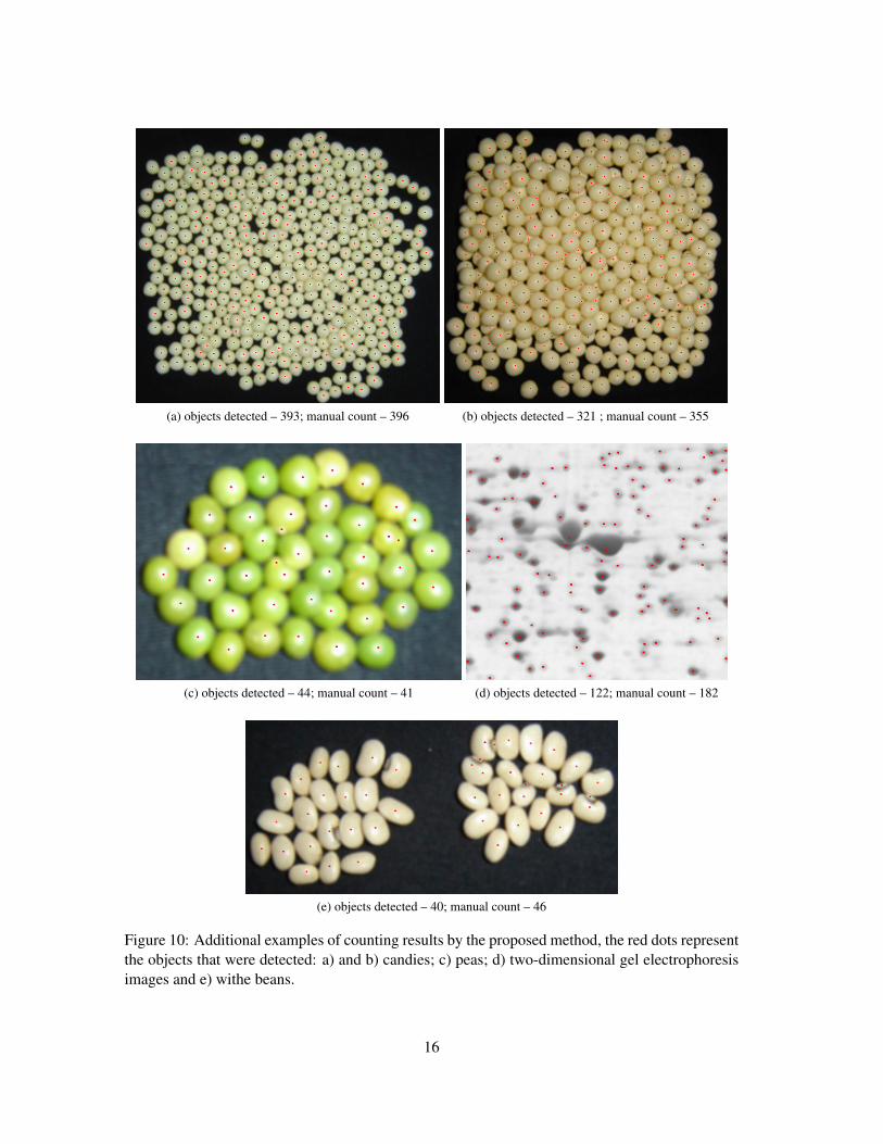
(a) objects detected – 393; manual count – 396 (b) objects detected – 321 ; manual count – 355

(c) objects detected – 44; manual count – 41 (d) objects detected – 122; manual count – 182

(e) objects detected – 40; manual count – 46

Figure 10: Additional examples of counting results by the proposed method, the red dots representthe objects that were detected: a) and b) candies; c) peas; d) two-dimensional gel electrophoresisimages and e) withe beans.

16

5 Conclusion and Future Works

In this work, an automatic method for detecting and counting stem cells sections obtained underfluorescence microscopy was presented. We handle with embryoid bodies obtained from embry-onic stem cells cultured in vitro. Our approach uses the luminance information to generate a graph-based image representation. Each cell was represented by a substructure that we called simple pathpattern. Then, a graph mining process is used to detect such pattern. The accuracy of the proposedmethod was demonstrated with experimental results in a large population of stem cells image. Theresults was validated by specialists from Institute of Biomedical Sciences – UFRJ/Brazil. We ob-tained an average precision, recall and F-measure of 93.97%, 92.04% and 92.87%, respectively,which is satisfactory. Moreover, with the automatic counting, we can eliminate the subjectivitybecause, unlike in manual counting, is guaranteed that the same criteria are always used to detectcells. In addition, the results obtained in another kinds of images demonstrate that the methodcould be used in others applications.

Most counting errors performed by the proposed method are due to the existence of more thanone lighter points at the same cell. Future work involves solving such problem by implementing anode contraction algorithm using their Euclidean distance as a criteria.

AcknowledgmentsThanks are due to Bruno Ávila and Aristófanes C. Silva for their most valuable assistance and to the teamof collaborators, specially Priscila Brito - student of Institute of Biomedical Sciences – UFRJ/Brazil. Theteam helped us in the algorithm validation, with some discussions around the research hypothesis. Theauthors are supported by CAPES.

References[1] B. Alberts, D. Bray, J. Lewis, M. Raff M, K. Roberts, and J. D. Watson. Molecular biology of the cell.

Garland Publishing Inc., (3), 1994.

[2] K. Althoff, J. Degerman, and T Gustavsson. Combined segmentation and tracking of neural stem-cells. In Image Analysis, pages 282 – 291. 2005.

[3] F. Ambriz-Colín, M. Torres-Cisneros, J. G. Avina-Cervantes, J. E. Saavedra-Martinez, O. Debeir, andJ. J. Sanchez-Mondragon. Detection of biological cells in phase-contrast microscopy images. InMICAI, pages 68 – 77, 2006.

[4] Dwi Anoraganingrum. Cell segmentation with median filter and mathematical morphology operation.In ICIAP, 1999.

[5] P. Bamford. Segmentation of cell images with an application to cervical cancer screening. PhD thesis,University of Queenland, 1999.

[6] A. Bieniek and A. Moga. An efficient watershed algorithm based on connected components.33(6):907–916, 2000.

[7] J. Degerman, J. Faijerson, K. Althoff, T. Thorlin, and T. Gustavsson. A comparative study betweenlevel set and watershed segmentations for tracking stem cells in time-lapse microscopy. In Workshopon Microscopic Image Analysis with Applications in Biology, pages 60 – 64, 2006.

[8] Takahashi et al. Induction of pluripotent stem cells from adult human fibroblasts by defined factors.Cell, 5(131):861 – 72, 2007.

17

[9] Lucena C. J. P. Faustino G., Gatti M. and Gattass M. A 3d multi-scale agent-based stem cell self-organization. SEAS, pages 37 – 48, 2008.

[10] Mark A. Foltz. Connected components in binary images. 6.866: Machine Vision, December 1997.

[11] A. Garrido and N. PeHrez de la Blanca. Applying deformable templates for cell image segmentation.Pattern Recognition, 33(5):821 – 832, 2000.

[12] E. Glory, A. Faure, V. Meas-Yedid, F. Cloppet, Ch Pinset, G. Stamon, and J-Ch Olivo-Marin. Aquantification tool to analyse stained cell cultures. In Image Analysis and Recognition, pages 84 – 91.2004.

[13] Minh-Tuan Trong Hoang and Yonggwan Won. A marker-free watershed approach for 2d-ge proteinspot segmentation. ISITC, pages 161 – 165, 2007.

[14] K. D. Iakovidis, E. Zacharia, and S. Kossida. A genetic approach to spot detection in two-dimensionalgel electrophoresis images. ITAB, 2006.

[15] N. N. Kachouie, P. Fieguth, and E. Jervis. Stem-cell localization: A deconvolution problem. In EMBS,pages 5525 – 5528, 2007.

[16] N. N. Kachouie, Paul Fieguth, John Ramunas, and Eric Jervis. Probabilisticmodel-based cell tracking.Int. Journal of Biomedical Imaging, pages 1 – 10, 2006.

[17] N. N. Kachouie, L. J. Lee, and P. Fieguth. A probabilistic living cell segmentation model. In ICIP,pages 137 – 140, 2005.

[18] N.N. Kachouie and P.W. Fieguth. A narrow-band level-set method with dynamic velocity for neuralstem cell cluster segmentation. In ICIAR, pages 1006–1013, 2005.

[19] N.N. Kachouie, P.W. Fieguth, J. Ramunas, and E. Jervis. A model-based hematopoietic stem celltracker. In ICIAR, pages 861–868, 2005.

[20] Anna Korzynska. Automatic counting of neural stem cells growing in cultures. In Computer Recog-nition Systems, pages 604 – 612. 2007.

[21] Julie Logan, Kirstin Edwards, and Nick Saunders. Real-Time PCR: Current Technology and Applica-tions. Caister Academic Press, 2009.

[22] Xi Long, W. Louis Cleveland, and Y. Lawrence Yao. Effective automatic recognition of cultured cellsin bright field images using fisher’s linear discriminant preprocessing. Image and Vision Computing,23(13):1203 – 1213, 2005.

[23] T. Markiewicz, S. Osowski, J. Patera, and W. Kozlowski. Image processing for accurate cell recog-nition and count on histologic slides. Int. Academy of Cytology and American Society of Cytology,28(5):281 – 291, 2006.

[24] Inkyu Moon and Bahram Javidi. Three-dimensional identification of stem cells by computationalholographic imaging. J. R. Soc. Interface, 4:305 – 313, 2006.

[25] Alexander Neubeck and Luc Van Gool. Efficient non-maximum suppression. In ICPR, volume 3,pages 850–855, 2006.

[26] Antti Niemisto, Limei Hu, Olli Yli-Harja, Wei Zhang, and Ilya Shmulevich. Quantification of in vitrocell invasion through image analysis. EMBS, pages 1 – 5, 2004.

[27] M. D. Stewart Sell. Stem Cells Handbook. Humana Press, 2003.

[28] S. Sergent-Tanguy, C. Chagneau, I. Neveu, and Naveilhan P . Fluorescent activated cell sorting (facs):a rapid and reliable method to estimate the number of neurons in a mixed population. Journal ofNeuroscience Methods, 129(1):73 – 79, 2003.

18

[29] H. Sheikh, Bin Zhu, and E. Micheli-Tzanakou. Blood cell identification using neural networks. InIEEE Twenty-Second Annual Northeast Bioengineering Conference, pages 119–120, 1996.

[30] S. Shiotani, T. Fukuda, F. Arai, N. Takeuchi, K. Sasaki, and T. Kinoshita. Cell recognition by imageprocessing: (recognition of dead or living plant cells by neural network). JSME, 37:202 – 208, 1994.

[31] Timthy Spencer, John A. Olson, Kenneth C. Mchardy, Peter R. Sharp, and John V. Forrester. Animage-processing strategy for the segmentation and quantification of microaneurysms in fluoresceinangiograms of the ocular fundus. Computers and Biomedical Researches, 29:284 – 302, 1996.

[32] C. Tang and E. Bengtsson. Segmentation and tracking of neural stem cell. In Advances in IntelligentComputing, pages 851–859. 2005.

[33] A. TREMEAU and P. COLANTONI. Regions adjacency graph applied to color image segmentation.EEE transactions on image processing, 9(4):735 – 744, 2000.

[34] Q. Zheng, B. K. Milthorpe, and A. S. Jones. Direct neural network application for automated cellrecognition. Cytometry A, 57(1):1–9, 2004.

[35] D. Zicha and G. Dann. Molecular biology of the cell. Journal of Microscopy, 3:11 – 21, 1995.

[36] C. Zimmer, E. Labruyère, V. Meas-Yedid, N. Guillén, and JC. Olivo-Marin. Improving active contoursfor segmentation and tracking of motile cells in videomicroscopy. 16th Int. Conference on PatterRecognition, 2:286 – 289, 2002.

19

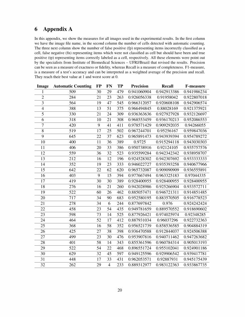
6 Appendix AIn this appendix, we show the measures for all images used in the experimental results. In the first columnwe have the image file name, in the second column the number of cells detected with automatic counting.The three next column show the number of false positive (fp) representing items incorrectly classified as acell, false negative (fn) representing items which were not classified as cell but should have been and truepositive (tp) representing items correctly labeled as a cell, respectively. All these elements were point outby the specialists from Institute of Biomedical Sciences – UFRJ/Brazil that revised the results. Precisioncan be seen as a measure of exactness or fidelity, whereas Recall is a measure of completeness. F1-measure,is a measure of a test’s accuracy and can be interpreted as a weighted average of the precision and recall.They reach their best value at 1 and worst score at 0.

Image Automatic Counting FP FN TP Precision Recall F-measure1 509 30 29 479 0.941060904 0.942913386 0.9419862342 284 21 23 263 0.926056338 0.91958042 0.9228070183 564 19 47 545 0.966312057 0.920608108 0.9429065744 388 13 51 375 0.966494845 0.88028169 0.9213759215 330 21 24 309 0.936363636 0.927927928 0.9321266976 318 10 21 308 0.968553459 0.936170213 0.9520865537 420 9 41 411 0.978571429 0.909292035 0.942660558 519 17 25 502 0.967244701 0.95256167 0.9598470369 645 22 37 623 0.965891473 0.943939394 0.95478927210 400 11 36 389 0.9725 0.915294118 0.94303030311 406 20 33 386 0.950738916 0.92124105 0.93575757612 559 36 32 523 0.935599284 0.942342342 0.93895870713 212 16 12 196 0.924528302 0.942307692 0.93333333314 352 19 23 333 0.946022727 0.935393258 0.94067796615 642 22 62 620 0.965732087 0.909090909 0.93655589116 403 9 15 394 0.977667494 0.963325183 0.9704433517 419 30 30 389 0.928400955 0.928400955 0.92840095518 276 16 21 260 0.942028986 0.925266904 0.93357271119 522 60 26 462 0.885057471 0.946721311 0.91485148520 717 34 90 683 0.952580195 0.883570505 0.91677852321 278 34 6 244 0.877697842 0.976 0.92424242422 458 23 54 435 0.949781659 0.889570552 0.91869060223 598 73 14 525 0.877926421 0.974025974 0.9234828524 464 52 17 412 0.887931034 0.96037296 0.92273236325 368 16 58 352 0.956521739 0.858536585 0.90488431926 425 27 38 398 0.936470588 0.912844037 0.92450638827 499 23 30 476 0.953907816 0.940711462 0.94726368228 401 58 14 343 0.855361596 0.960784314 0.90501319329 522 54 22 468 0.896551724 0.955102041 0.92490118630 629 32 45 597 0.949125596 0.929906542 0.93941778131 448 17 33 431 0.962053571 0.92887931 0.94517543932 262 29 4 233 0.889312977 0.983122363 0.933867735

20

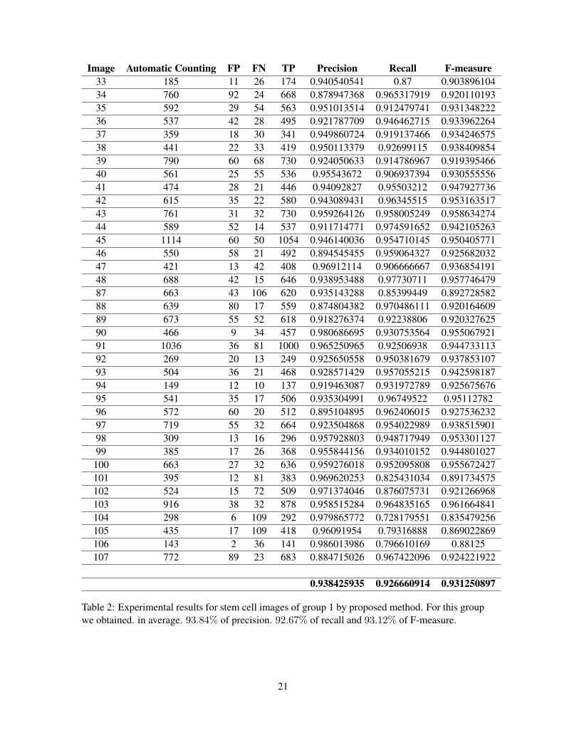
Image Automatic Counting FP FN TP Precision Recall F-measure33 185 11 26 174 0.940540541 0.87 0.90389610434 760 92 24 668 0.878947368 0.965317919 0.92011019335 592 29 54 563 0.951013514 0.912479741 0.93134822236 537 42 28 495 0.921787709 0.946462715 0.93396226437 359 18 30 341 0.949860724 0.919137466 0.93424657538 441 22 33 419 0.950113379 0.92699115 0.93840985439 790 60 68 730 0.924050633 0.914786967 0.91939546640 561 25 55 536 0.95543672 0.906937394 0.93055555641 474 28 21 446 0.94092827 0.95503212 0.94792773642 615 35 22 580 0.943089431 0.96345515 0.95316351743 761 31 32 730 0.959264126 0.958005249 0.95863427444 589 52 14 537 0.911714771 0.974591652 0.94210526345 1114 60 50 1054 0.946140036 0.954710145 0.95040577146 550 58 21 492 0.894545455 0.959064327 0.92568203247 421 13 42 408 0.96912114 0.906666667 0.93685419148 688 42 15 646 0.938953488 0.97730711 0.95774647987 663 43 106 620 0.935143288 0.85399449 0.89272858288 639 80 17 559 0.874804382 0.970486111 0.92016460989 673 55 52 618 0.918276374 0.92238806 0.92032762590 466 9 34 457 0.980686695 0.930753564 0.95506792191 1036 36 81 1000 0.965250965 0.92506938 0.94473311392 269 20 13 249 0.925650558 0.950381679 0.93785310793 504 36 21 468 0.928571429 0.957055215 0.94259818794 149 12 10 137 0.919463087 0.931972789 0.92567567695 541 35 17 506 0.935304991 0.96749522 0.9511278296 572 60 20 512 0.895104895 0.962406015 0.92753623297 719 55 32 664 0.923504868 0.954022989 0.93851590198 309 13 16 296 0.957928803 0.948717949 0.95330112799 385 17 26 368 0.955844156 0.934010152 0.944801027100 663 27 32 636 0.959276018 0.952095808 0.955672427101 395 12 81 383 0.969620253 0.825431034 0.891734575102 524 15 72 509 0.971374046 0.876075731 0.921266968103 916 38 32 878 0.958515284 0.964835165 0.961664841104 298 6 109 292 0.979865772 0.728179551 0.835479256105 435 17 109 418 0.96091954 0.79316888 0.869022869106 143 2 36 141 0.986013986 0.796610169 0.88125107 772 89 23 683 0.884715026 0.967422096 0.924221922

0.938425935 0.926660914 0.931250897

Table 2: Experimental results for stem cell images of group 1 by proposed method. For this groupwe obtained. in average. 93.84% of precision. 92.67% of recall and 93.12% of F-measure.

21

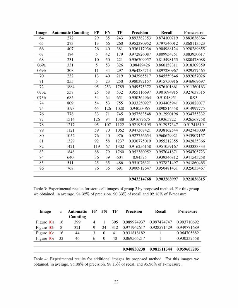
Image Automatic Counting FP FN TP Precision Recall F-measure64 272 29 35 243 0.893382353 0.874100719 0.88363636465 273 13 66 260 0.952380952 0.797546012 0.86811352366 407 26 40 381 0.936117936 0.904988124 0.92028985567 184 5 42 179 0.972826087 0.809954751 0.88395061768 231 10 50 221 0.956709957 0.815498155 0.880478088

069a 331 5 53 326 0.98489426 0.860158311 0.918309859069b 308 11 34 297 0.964285714 0.897280967 0.929577465

70 232 13 40 219 0.943965517 0.845559846 0.89205702671 255 5 23 250 0.980392157 0.915750916 0.94696969772 1884 95 253 1789 0.949575372 0.876101861 0.911360163

073a 557 25 58 532 0.955116697 0.901694915 0.927637315073b 685 34 64 651 0.950364964 0.91048951 0.93

74 809 54 53 755 0.933250927 0.934405941 0.93382807775 1093 65 126 1028 0.94053065 0.890814558 0.91499777576 778 33 71 745 0.957583548 0.912990196 0.93475533277 1514 126 94 1388 0.91677675 0.9365722 0.92656875878 1217 95 107 1122 0.921939195 0.912937347 0.9174161979 1121 59 70 1062 0.947368421 0.938162544 0.94274300980 1052 76 40 976 0.927756654 0.960629921 0.94390715781 1329 92 58 1237 0.930775019 0.955212355 0.94283536682 1421 119 67 1302 0.916256158 0.951059167 0.93333333383 1848 88 79 1760 0.952380952 0.957041871 0.95470572384 640 36 39 604 0.94375 0.939346812 0.94154325885 511 25 35 486 0.951076321 0.932821497 0.94186046586 767 76 36 691 0.900912647 0.950481431 0.925033467

0.943214768 0.903263997 0.921836315

Table 3: Experimental results for stem cell images of group 2 by proposed method. For this groupwe obtained. in average. 94.32% of precision. 90.33% of recall and 92.18% of F-measure.

Image ε Automatic FP FN TP Precision Recall F-measureCounting

Figure 10a 16 399 4 1 395 0.989974937 0.997474747 0.993710692Figure 10b 8 321 9 24 312 0.971962617 0.928571429 0.949771689Figure 10c 16 44 3 0 41 0.931818182 1 0.964705882Figure 10e 32 46 6 0 40 0.869565217 1 0.930232558

0.940830238 0.981511544 0.959605205

Table 4: Experimental results for additional images by proposed method. For this images weobtained. in average. 94.08% of precision. 98.15% of recall and 95.96% of F-measure.

22