UU-NF 07#05 (March 2007)

UPPSALA UNIVERSITY NEUTRON PHYSICS REPORT ISSN 1401-6269

AUTOMATIC GAMMA-SCANNING SYSTEM FOR MEASUREMENT OF

RESIDUAL HEAT IN SPENT NUCLEAR FUEL

OTASOWIE OSIFO

LICENTIATE THESIS

UPPSALA UNIVERSITY DEPARTMENT OF NEUTRON RESEARCH

PROGRAM OF APPLIED NUCLEAR PHYSICS UPPSALA, SWEDEN

UU-NF 07#05 (March 2007) UPPSALA UNIVERSITY NEUTRON PHYSICS REPORT

ISSN 1401-6269

Editor: J Källne

AUTOMATIC GAMMA-SCANNING SYSTEM FOR

MEASUREMENT OF RESIDUAL HEAT IN SPENT

NUCLEAR FUEL

OTASOWIE OSIFO

Department of Neutron Research, Uppsala University,

BOX 525, SE-75120 Uppsala, Sweden

Abstract

In Sweden, spent nuclear fuel will be encapsulated and placed in a deep geological repository. In

this procedure, reliable and accurate spent fuel data such as discharge burnup, cooling time and

residual heat must be available. The gamma scanning method was proposed in earlier work as a

fast and reliable method for the experimental determination of such spent fuel data.

This thesis is focused on the recent achievements in the development of a pilot gamma

scanning system and its application in measuring spent fuel residual heat. The achievements

include the development of dedicated spectroscopic data-acquisition and analysis software and

the use of a specially designed calorimeter for calibrating the gamma scanning system.

The pilot system is described, including an evaluation of the performance of the spectrum

analysis software. Also described are the gamma-scanning measurements on 31 spent PWR fuel

assemblies performed using the pilot system. The results obtained for the determination of

residual heat are presented, showing an agreement of (2-3) % with both calorimetric and

calculated data. In addition, the ability to verify declared data such as discharge burnup and

cooling time is demonstrated.

UPPSALA UNIVERSITY DEPARTMENT OF NEUTRON RESEARCH

PROGRAM OF APPLIED NUCLEAR PHYSICS UPPSALA, SWEDEN

This licentiate thesis is based on the following papers: Paper I Data acquisition and analysis software for rapid gamma scanning: application for the verification of spent LWR fuel parameters O. Osifo, A. Håkansson, S. Jacobsson Svärd, A. Bäcklin To be submitted to Nuclear Instruments and Methods in Physics Research A A pilot gamma scanning system is being developed as part of the research and development program for the planned spent nuclear fuel encapsulation plant in Sweden. For this system, a software package has been developed with modules for fast automatic repetition of spectrum acquisition and consecutive spectrum analysis. The software is also able to interact with a database of fuel information, including operator-declared data and measured data.

The software package has been used in the gamma scanning of spent PWR fuel assemblies at the interim storage facility for spent nuclear fuel (CLAB) in Oskarshamn, Sweden. Results obtained from the measurements are presented. The analyses showing that fuel burnup, cooling time and residual heat can be verified within (2-3) % (1 σ). Paper II Verification and determination of the decay heat in spent PWR fuel by means of gamma scanning O. Osifo, S. Jacobsson Svärd, A. Håkansson, C. Willman, A. Bäcklin, T. Lundqvist Submitted to Nuclear Science and Engineering Decay heat is an important design parameter at the future Swedish spent nuclear fuel repository. It will be calculated for each fuel assembly using dedicated depletion codes, based on the operator-declared irradiation history. However, experimental verification of the calculated decay heat is also anticipated. Such verification may be obtained by gamma scanning, using the established correlation between the decay heat and the emitted gamma-ray intensity from 137Cs. In this procedure, also the correctness of the operator-declared fuel parameters may be verified.

Recent achievements of the gamma scanning technique include the development of a dedicated spectroscopic data-acquisition system and the use of an advanced calorimeter for calibration. Using this system, the operator-declared burnup and cooling time of 31 PWR fuel assemblies was verified experimentally to within 2.2% (1 σ) and 1.9 % (1 σ), respectively. The measured decay heat agreed with calorimetric data within 2.3% (1 σ), whereby the calculated decay heat was verified within 2.3 % (1 σ). The measuring time per fuel assembly was about 15 minutes.

In case reliable operator-declared data is not available, the gamma-scanning technique also provides a means to independently measure the decay heat. The results obtained in this procedure agreed with calorimetric data within 2.7 % (1 σ).

1

Table of contents 1 Management of spent nuclear fuel in Sweden ................................................................... 3

1.1 The once-through nuclear fuel cycle.......................................................................... 3 1.1.1 The front end ...................................................................................................... 3 1.1.2 Reactor operation ............................................................................................... 4 1.1.3 The back end ...................................................................................................... 5

1.2 Operational margins at a final repository................................................................... 6 2 Spent fuel and its discharge parameters ............................................................................. 7

2.1 Fuel types ................................................................................................................... 7 2.2 Discharge burnup ....................................................................................................... 8 2.3 Cooling time............................................................................................................... 9 2.4 Reactivity ................................................................................................................... 9

3 Residual heat ...................................................................................................................... 9 3.1 Origin of residual heat.............................................................................................. 10 3.2 Dependence of residual heat on spent fuel parameters ............................................ 10

3.2.1 Dependence on cooling time ............................................................................ 10 3.2.2 Dependence on burnup..................................................................................... 12

4 Methods of determination of residual heat....................................................................... 12 4.1 Computational methods............................................................................................ 13 4.2 Calorimetry............................................................................................................... 13 4.3 Gamma scanning ...................................................................................................... 17

4.3.1 Principles of the method................................................................................... 17 4.3.2 Application of the method in this work............................................................ 17 4.3.3 The fractional contribution, f ........................................................................... 18

5 Gamma scanning equipment ............................................................................................ 18 5.1 The mechanical equipment....................................................................................... 18 5.2 The detector and the pc-based data-acquisition system ........................................... 19 5.3 The software............................................................................................................. 20

5.3.1 The data-acquisition software .......................................................................... 20 5.3.2 The spectrum analysis software ....................................................................... 20 5.3.3 Application of the software: spent fuel parameters.......................................... 21

6 Experimental studies ........................................................................................................ 22 6.1 Overview of the measurement procedure................................................................. 22 6.2 Calibration and normalization.................................................................................. 22 6.3 Determination of discharge burnup and cooling time.............................................. 23 6.4 Verification of calculated residual heat.................................................................... 23 6.5 Determination of residual heat ................................................................................. 23 6.6 Discussion of the experimental uncertainty ............................................................. 23

7 Conclusions and outlook .................................................................................................. 24 8 Acknowledgements .......................................................................................................... 25 References ................................................................................................................................ 25

2

1 Management of spent nuclear fuel in Sweden In Sweden, about 50 % [1] of the electrical power is generated by nuclear power. The reactors at the power stations are all light water reactors (LWR). Of these, 3 are pressurized water reactors (PWR) and 7 are boiling water reactors (BWR). The operation of these reactors gives rise to the production of radioactive waste in the form of spent nuclear fuel and related by-products. The waste has to be managed in such a way as to fulfil national and international safety and security requirements. The method for managing spent nuclear fuel depends on the strategy chosen by each country for its nuclear fuel cycle. In Sweden, the strategy is based on the once-through fuel cycle (also called the open cycle) that implies that no part of the spent fuel is reprocessed or recycled [2, 3]. The different stages in this fuel cycle are described below.

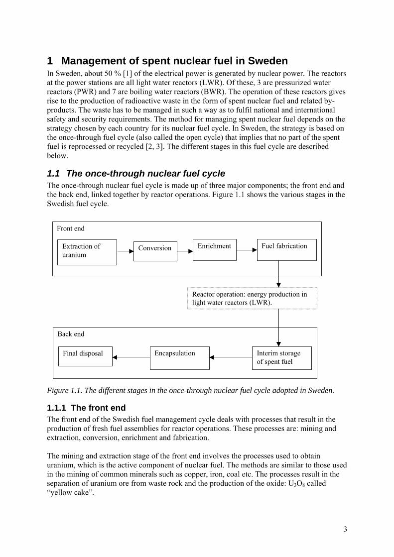
1.1 The once-through nuclear fuel cycle The once-through nuclear fuel cycle is made up of three major components; the front end and the back end, linked together by reactor operations. Figure 1.1 shows the various stages in the Swedish fuel cycle.

Front end

Extraction of uranium

Conversion

Enrichment Fuel fabrication

Reactor operation: energy production in light water reactors (LWR).

Back end

Encapsulation

Interim storage of spent fuel

Final disposal

Figure 1.1. The different stages in the once-through nuclear fuel cycle adopted in Sweden.

1.1.1 The front end The front end of the Swedish fuel management cycle deals with processes that result in the production of fresh fuel assemblies for reactor operations. These processes are: mining and extraction, conversion, enrichment and fabrication. The mining and extraction stage of the front end involves the processes used to obtain uranium, which is the active component of nuclear fuel. The methods are similar to those used in the mining of common minerals such as copper, iron, coal etc. The processes result in the separation of uranium ore from waste rock and the production of the oxide: U3O8 called “yellow cake”.

3

In the conversion stage, the yellow cake is purified and converted to gaseous uranium hexafluoride (UF6).

Natural uranium is mainly composed of two isotopes: 235U (0.72 %) and 238U (99.27 %). However, for use in a light water reactor, the amount of the fissile isotope 235U has to be increased. This is done through the enrichment process, which results in the production of low enriched uranium in the form of uranium hexaflouride gas with an enrichment in 235U of typically 3 –5 %.

In the fuel fabrication stage, the enriched uranium hexaflouride gas is used to produce uranium dioxide (UO2) powder, which is sintered into fuel pellets. The pellets are stacked together in thin tubes made from a zirconium alloy to form fuel rods, which are assembled in a square matrix to form the fuel assemblies. The number of fuel rods differs between fuel types or fuel geometries. The assemblies also contain structural materials that may be different for different fuel types and geometries. Examples of different fuel types are shown in section 2.1.

1.1.2 Reactor operation Each nuclear power reactor contains several hundreds of fuel assemblies that make up the reactor core. In the core, heat is produced through the fission reaction that occurs mainly in 235U. The heat generated through fission is used to produce steam, which is used to drive turbines. The mechanical energy of the turbines is transformed into electrical energy by generators. In a reactor, neutrons initiate each fission reactions and the resulting products are, on the average, 2.4 neutrons and two fission fragments (fission products). The neutrons that are produced in the fission reaction must slow down via moderation to reach thermal energies, i.e. kinetic energies corresponding to the temperature of the surroundings. For light water reactors, such moderation is obtained in the cooling water surrounding the fuel assemblies. Due to this specific function, the cooling water is also denoted moderator. If a sufficiently large fraction of the fission neutrons survive, these can cause new fission reactions and a self-sustaining chain reaction is achieved. Under this condition, the rate of production of neutrons is equal to the total rate of loss of neutrons from the core and capture in the fuel itself. The condition is expressed mathematically as [4]:

1 ( )eff

Total rate of loss of neutrons Rate of production of neutronsk

= × (1.1)

Where the quantity keff is called the effective neutron multiplication constant. If keff = 1, a self-sustaining chain reaction is maintained and the core is said to be critical. When keff < 1, the core is sub-critical implying that it cannot maintain a self-sustaining chain reaction. When keff > 1 a supercritical core is obtained implying power excursions in the core. Besides fission, several other nuclear reactions such as radiative capture of neutrons occur in the fuel leading to the production of such actinides as 239Pu and activation products such as 60Co in the structural materials. Due to the fission process, the amount of fissile 235U in the fuel decreases with time and, accordingly, a fraction (about 25 % [5]) of the fuel assemblies is discharged from the core every year and replaced with fresh fuel assemblies (refuelling).

4

The isotopes produced in the fuel by fission and by other nuclear reactions, are in general radioactive with half-lives ranging from seconds to thousands of years. The resulting inventory of radioactive materials in irradiated fuel assemblies has a great impact on the rate of residual heat production, the time scales and the safety strategies adopted in the back end of the once-through fuel cycle.

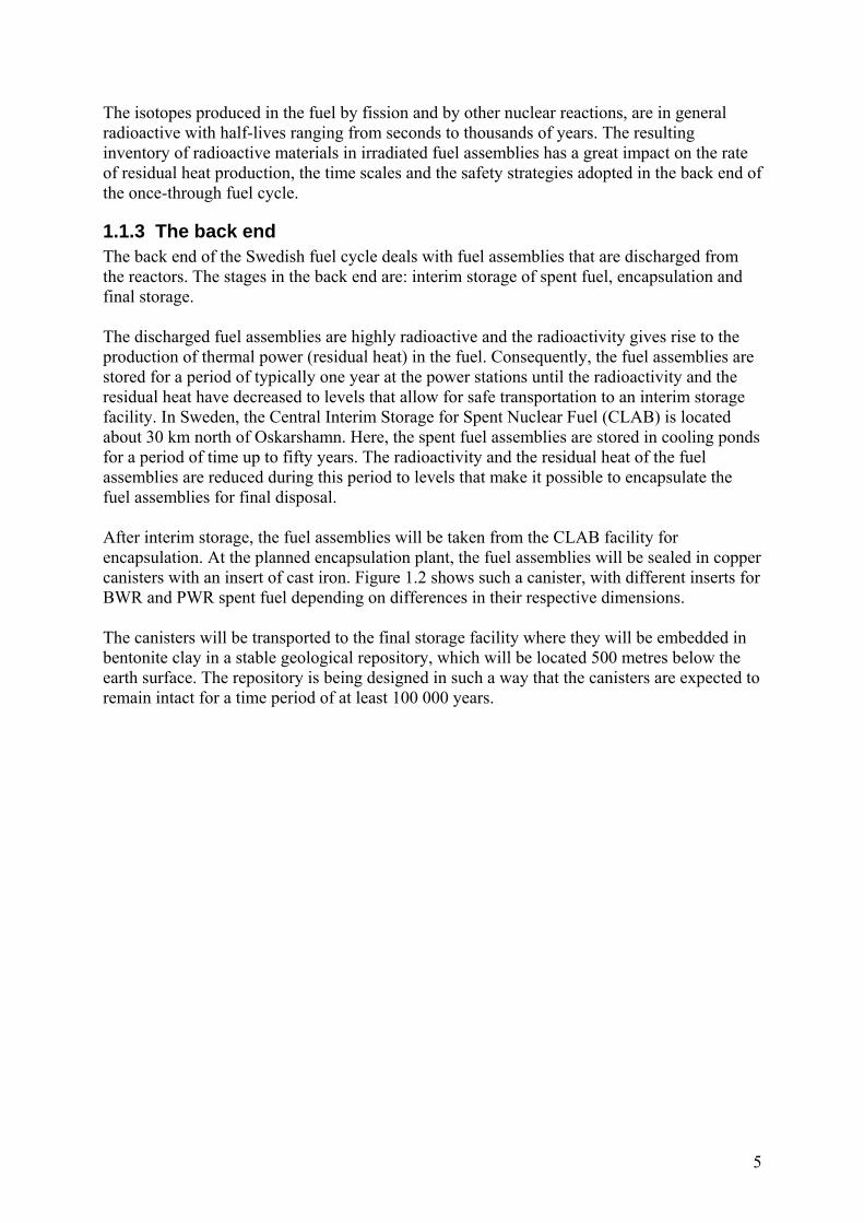
1.1.3 The back end The back end of the Swedish fuel cycle deals with fuel assemblies that are discharged from the reactors. The stages in the back end are: interim storage of spent fuel, encapsulation and final storage. The discharged fuel assemblies are highly radioactive and the radioactivity gives rise to the production of thermal power (residual heat) in the fuel. Consequently, the fuel assemblies are stored for a period of typically one year at the power stations until the radioactivity and the residual heat have decreased to levels that allow for safe transportation to an interim storage facility. In Sweden, the Central Interim Storage for Spent Nuclear Fuel (CLAB) is located about 30 km north of Oskarshamn. Here, the spent fuel assemblies are stored in cooling ponds for a period of time up to fifty years. The radioactivity and the residual heat of the fuel assemblies are reduced during this period to levels that make it possible to encapsulate the fuel assemblies for final disposal. After interim storage, the fuel assemblies will be taken from the CLAB facility for encapsulation. At the planned encapsulation plant, the fuel assemblies will be sealed in copper canisters with an insert of cast iron. Figure 1.2 shows such a canister, with different inserts for BWR and PWR spent fuel depending on differences in their respective dimensions. The canisters will be transported to the final storage facility where they will be embedded in bentonite clay in a stable geological repository, which will be located 500 metres below the earth surface. The repository is being designed in such a way that the canisters are expected to remain intact for a time period of at least 100 000 years.

5

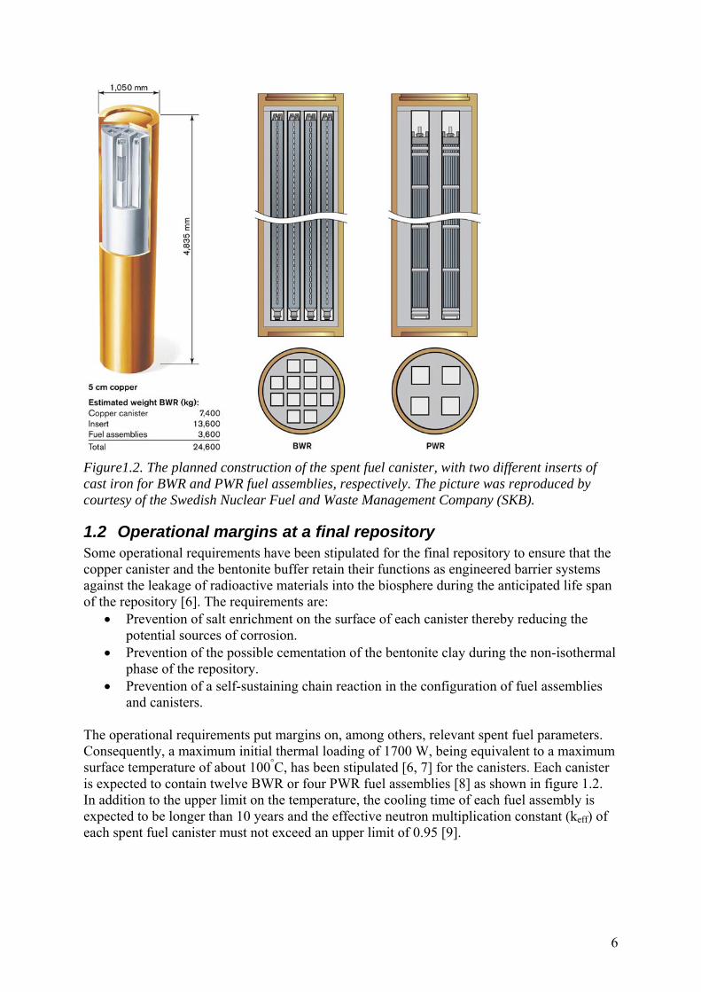
Figure1.2. The planned construction of the spent fuel canister, with two different inserts of cast iron for BWR and PWR fuel assemblies, respectively. The picture was reproduced by courtesy of the Swedish Nuclear Fuel and Waste Management Company (SKB).

1.2 Operational margins at a final repository Some operational requirements have been stipulated for the final repository to ensure that the copper canister and the bentonite buffer retain their functions as engineered barrier systems against the leakage of radioactive materials into the biosphere during the anticipated life span of the repository [6]. The requirements are:

• Prevention of salt enrichment on the surface of each canister thereby reducing the potential sources of corrosion.

• Prevention of the possible cementation of the bentonite clay during the non-isothermal phase of the repository.

• Prevention of a self-sustaining chain reaction in the configuration of fuel assemblies and canisters.

The operational requirements put margins on, among others, relevant spent fuel parameters. Consequently, a maximum initial thermal loading of 1700 W, being equivalent to a maximum surface temperature of about 100°C, has been stipulated [6, 7] for the canisters. Each canister is expected to contain twelve BWR or four PWR fuel assemblies [8] as shown in figure 1.2. In addition to the upper limit on the temperature, the cooling time of each fuel assembly is expected to be longer than 10 years and the effective neutron multiplication constant (keff) of each spent fuel canister must not exceed an upper limit of 0.95 [9].

6

Furthermore, the International Atomic Energy Agency (IAEA) recommends that the following information should be available for the safe management of interim storage facilities [10]:

• Fuel designs, including scale drawings. • Materials of fuel construction, including initial and final mass of all fissile contents. • Fuel identification numbers. • Fuel history (e.g. burnup, reactor power rating during irradiation, residual heat and

dates of loading and discharge from the core). • Details of conditions present that can affect fuel storage (e.g. damage to fuel cladding

or structural damage etc). One consequence of the above requirements and operational margins is the need for methods that can be used to verify the operator declared spent fuel data.

2 Spent fuel and its discharge parameters The discharge parameters that are addressed in this work are fuel designs, discharge burnup, cooling time and, being the major focus of this work, the residual heat. These parameters are described below.

2.1 Fuel types For light water reactors, there are two major types of fuel assemblies: PWR and BWR. These major fuel types can be divided into subgroups according to the manufacturer, the number of rods in the square matrix, the design of the structural materials that make up the fuel, presence of control rod clusters, presence of water and instrument channels, etc. In this work, only two PWR fuel types have been considered: the KWU15x15 type with 204 fuel rods and the Westinghouse 17x17 type with 264 fuel rods. Figure 2.1 shows examples of a PWR and a BWR fuel type. As can be seen in the figure, the fuel types exhibit both physical and structural differences that have consequences for both core physics and radiation measurement systems. One example of such structural difference is the fuel channel that surrounds the BWR fuel bundle, which is not present in PWR fuel assemblies.

7

Figure 2.1. Examples of a BWR and a PWR fuel assembly. The fuel geometries are of the Svea 96 and 17x17 types, respectively. The picture was reproduced by courtesy of the Swedish Nuclear Fuel and Waste Management Company (SKB).

2.2 Discharge burnup Fuel burnup can be defined as the quantity of fission energy produced per mass of nuclear fuel during its residence time in the core [4]. The fuel discharge burnup is known as exposure and for commercial power reactors; it is measured in Gigawatt-days per metric tonne of uranium (GWd/tU). It can also be defined as the ratio between the total number of atoms of uranium fissioned and the total number of uranium present initially. For the purpose of assessment of spent fuel characteristics, the burnup can be related to the amount of each isotope produced in the fuel during irradiation. It can also be used as an indirect measure of the amount of fissile uranium remaining in the fuel for the purpose of estimating the reactivity of the spent fuel, see section 2.4. Given a certain irradiation scheme, a functional relationship can be established between the discharge burnup and the amount of each of the radioisotopes produced in the fuel. In particular, figure 2.2 shows that the amount of 137Cs produced in an irradiated fuel assembly is proportional to the burnup.

8

0 10 20 30 40 50 600

50

100

150

200

250

300

350

400

Burnup [GWd/tU]

Mas

s of

137 C

s [g

]

Figure 2.2. The dependence of the amount of 137Cs produced in an irradiated fuel assembly on the burnup. The data was obtained from computations with the ORIGEN-ARP depletion code.

This fact is relevant in this work because it shows that the burnup can be determined from the amount of the fission product 137Cs present in the fuel at discharge.

2.3 Cooling time The cooling time is the length of time from the discharge of a fuel assembly from the reactor core to the present. Due to the decay of the radioactive isotopes in the fuel, the inventory of the fission products and actinides will change with cooling time.

2.4 Reactivity Spent fuel contains fissile materials such as 239Pu produced in the fuel during irradiation. In spent fuel storage, the fissile isotopes can undergo fissions triggered by neutrons from spontaneous fissionable nuclei such as 244Cm. Such processes could potentially result in a critical configuration. For criticality to occur, the following conditions must be satisfied: the presence of sufficient quantities of fissile materials, suitable arrangement of the materials and the presence of neutrons of appropriate energies. Before the disposal of a spent fuel canister, its reactivity must be assessed to ensure that the conditions for avoiding criticality will be fulfilled.

3 Residual heat As discussed in section 1.2, residual heat is one of the important spent fuel parameters for the safe operation of a spent fuel storage facility. The residual heat of irradiated fuel assemblies is made up of two major components; decay heat and fission heat. In the final storage facility, the fuel canisters will remain subcritical and accordingly heat production in the repository will be dominated by decay heat.

9

3.1 Origin of residual heat The production of heat in the decay processes is due to the loss of kinetic energy by the emitted particles and gamma radiation. This process can be expressed mathematically as a sum over all decaying nuclei:

M

i i ii=1

P(t) = λ N (t)E∑ (3.1)

Where P(t) is the average rate of heat production in the fuel at time t after discharge, Ni(t) is the amount of the atoms of isotope i in the fuel at the time t, λi is the decay constant of the isotope i and Ei is the average energy released per disintegration of the radioisotope i. There is also a contribution to the residual heat from induced fission, which occurs due to neutrons emitted in e.g spontaneous fission. However, under the subcritical conditions of a final repository, this contribution may be neglected.

3.2 Dependence of residual heat on spent fuel parameters The isotopic content of the fuel at a cooling time T depends on fuel parameters such as burnup, irradiation history and initial enrichment in 235U. This implies that the residual heat also depends on these parameters and, as discussed below, the burnup and the cooling time of a spent fuel assembly have significant influence on the thermal loading of the spent fuel canisters after encapsulation.

3.2.1 Dependence on cooling time Due to decay, the contribution from each isotope to the residual heat of the spent fuel varies with time after discharge. To illustrate this, figure 3.1 shows the total residual heat and the heat contribution from the actinides and the fission products in a PWR 17x17 spent fuel assembly with a discharge burnup of 40 GWd/tU and an initial enrichment of 3.10 %. The data shown in figure 3.1 indicate that fission products initially dominate the residual heat while the long-lived actinides dominate the residual heat for cooling times exceeding 100 years. This attribute is due to the fact that the actinides generally possess long half-lives and long decay chains while the opposite generally holds for fission products.

10

10

110

210

310

410

5

10-2

100

102

104

Cooling time [years]

Resi

dual

hea

t [W

]Actinides residual heat Fission products residual heatTotal residual heat

Figure 3.1. The residual heat of a PWR 17X17 spent fuel assembly during the life span of the repository. The discharge burnup of the fuel assembly was 40 GWd/tU while the initial enrichment was 3.1 %. The data was obtained from calculations using ORIGEN-ARP.

As shown in figure 3.1, the residual heat decreases continuously. This implies that if the stated limit of the residual heat is maintained at the time of encapsulation, it will not be violated during the lifespan of the repository. At a typical cooling time of 30 years for encapsulation, the major contributors to the residual heat are radioisotopes with half-lives ranging from tens of years to a few hundred years: 137Cs + 137mBa, 90Sr + 90Y, 238Pu, 244Cm and 241Am. This is illustrated in figure 3.2

28%

33%

14%

13%

7%5%

Sr-90 + Y-90Cs-137 + Ba-137Am-241Pu-238Cm-244Other isotopes

Figure 3.2. The contributions of the isotopes: 137Cs + 137Ba, 90Sr + 90Y, 241Am, 238Pu and 244Cm to the residual heat of a spent fuel assembly at a cooling time of 30 years. The data was obtained from ORIGEN-ARP computations for a PWR 17X17 fuel assembly with a burnup of 40 GWd/tU and an initial enrichment of 3.1 %. The residual heat was 980 W/tU.

11

As seen in figure 3.2, the decay of the isotope 137Cs and its short-lived daughter 137mBa contributes about 33 % to the residual heat of the spent fuel. This characteristic is relevant for the gamma spectroscopic method of determination of residual heat that is discussed in section 4.3.

3.2.2 Dependence on burnup The residual heat of a spent fuel assembly depends not only on the cooling time but also on the discharge burnup. In figure 3.3 the residual heat is shown for different cooling times for a fuel burnup of 16 GWd/tU, 26 GWd/tU, 33 GWd/tU, 40 GWd/tU and 49 GWd/tU, respectively. The consequence of the trends shown figure 3.3 is that fuel assemblies with high burnup may require a longer cooling time in order to satisfy the criteria for thermal loading at the time of encapsulation.

10 15 20 25 30 35 40 45 50

500

1000

1500

2000

2500

Cooling time [years]

Resi

dual

hea

t [W

/tU]

Canister average16 GWd/tU 26 GWd/tU 33 GWd/tU 40 GWd/tU 49 GWd/tU

Figure 3.3. The residual heat at a cooling time period of 10-53 years for a fuel burnup of 16 GWd/tU, 26 GWd/tU, 33 GWd/tU, 40 GWd/tU and 49 GWd/tU, respectively. Also shown is the upper limit of the average thermal loading when placing four PWR assemblies in a canister.

A spent fuel canister can contain a maximum of four PWR fuel assemblies, corresponding to about 1840 kg uranium. Hence a maximum limit of 1700 W per canister is equal to an average thermal loading of 924 W/tU. This limit is illustrated in figure 3.3 and it indicates the need for accurate and reliable spent fuel data.

4 Methods of determination of residual heat Currently, three methods are used to determine the residual heat of spent nuclear fuel assemblies: computational methods, calorimetry and the gamma ray spectroscopic method. These methods are described below.

12

4.1 Computational methods The residual heat of spent nuclear fuel assemblies can be determined by using various computational codes. Three main types of such codes are described:

• Methods that are based on creating simple analytic expressions for the residual heat by using simulated data for spent fuel assemblies [11, 12]. Parametric expressions are developed in terms of spent fuel discharge parameters such as burnup, cooling time, initial enrichment of 235U, total number of irradiation days and total number of outage days. These codes can be used to determine residual heat with accuracies in the region of 8 %.

• Methods that yield the residual heat by solving the generalized Bateman equations either analytically or numerically [13]. The irradiation periods as well as the cooling time are taken into consideration in estimating the inventory of radioactive isotopes in the spent fuel. The contribution to the residual heat is obtained by summation according to eq. 3.1. An example of such a code is ORIGEN-ARP, which has accuracy in the range of 2-5 % (1 σ) [14].

• Methods that are coupled to lattice cell and nodal analysis codes such as CASMO and SIMULATE. The inventory of radioactive isotopes for a spent fuel assembly at the point of discharge is obtained from these codes. By taking into account the radioactive decay for each isotope, the contribution to the residual heat is obtained from summation according to eq. 3.1. An example of a code in which this method is implemented is the SNF fuel back end code from Studsvik Scandpower [15]. The calculated residual heat presented in paper II has been obtained using the SNF code. The accuracy is in the range of 2-3 % (1 σ) [16].

It can be noted that the results obtained with computational codes are highly dependent on the reliability of the input data used in the calculations such as irradiation history, discharge burnup, initial enrichment and cooling time. Due to this dependency it is advisable to resort to an experimental method, at least in order to be able to verify the calculated results. In the following two sections two measuring methods are briefly presented.

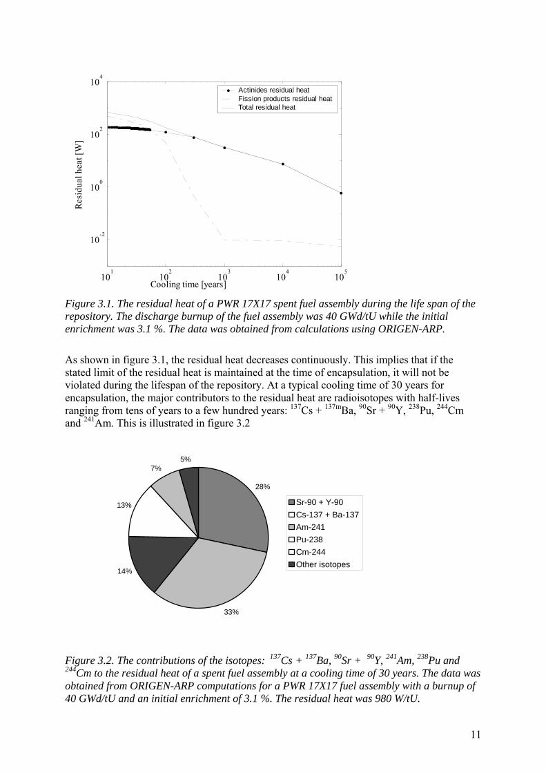
4.2 Calorimetry The calorimeter is the basic instrument for measuring the rate at which heat is generated by a body. Calorimeters are used for measurements in diverse applications that range from heat of chemical reactions to dose rate measurements in nuclear reactors. The type of calorimeter that is widely used for radiometric measurement is the heat flow/isothermal calorimeter. A schematic diagram of the system that was used for collecting the calorimetric data on the residual heat that is included in paper II is shown in figure 4.1.

13

Figure 4.1. A schematic picture of the radiometric calorimeter system used to measure the residual heat of spent fuel assemblies at the CLAB facility in Sweden.

The calorimeter was designed for the measurement of spent fuel residual heat at the CLAB facility in Sweden. It can be used for the measurement of residual heat in the range of 50 W to 1 kW with a projected accuracy of 2 % (2 σ) for both BWR and PWR fuel assemblies [17, 18]. It is located in one of the pools in the spent fuel reception area at the CLAB facility. It is made up of the following components: a sample measurement chamber that contains water as the heat transfer medium, a thermal barrier and a surrounding heat sink. During measurements, the fuel assembly is placed in the measurement chamber at a temperature Tm while the heat sink is maintained at a temperature T0. Here, the rate of heat generation from radioactive decay is assumed to be constant over the measurement period resulting in the general heat balance equation for the system given by [19, 20, 21]:

14

[mm 0 m 0

dTC = P + P - k(T - T )dt

] (4.1)

Where t denotes time, Pm is the power generated by the fuel assembly, P0 is the power added to the system by the recirculation pump, C is a calibration constant that is related to the heat capacity of the material in the measurement chamber and k is the coefficient of heat transfer through the measurement chamber. The calorimetric measurements can be performed in three modes: the steady state mode, the circulation mode and the temperature rise mode. However, the time required to perform one measurement is very long for both the steady state mode and the circulation mode. Hence the temperature rise mode is used for residual heat measurements at CLAB [17]. In this procedure, the measurement chamber is cooled a few degrees Celsius below the temperature T0 of the heat sink. The fuel assembly is then introduced into the measurement chamber and the temperature Tm is allowed to increase a few degrees Celsius above T0. By measuring the rate of temperature rise in the vicinity of Tm = T0, the residual heat of the fuel assembly is obtained from eq. 4.1 according to:

mm

dTP = C - Pdt 0 (4.2)

The constant C is obtained in a calibration procedure by using an electric heating element that was designed in the form of a BWR fuel assembly. Figure 4.2 shows a plot of the temperature rise as a function of time when the calorimeter was cooled 1.5 degree Celsius below the temperature T0 . The data shown was obtained with the heating element adjusted to 150 W.

0 1 2 3 4 5 6 7-2

-1.5

-1

-0.5

0

0.5

1

1.5

Time [hours]

Tem

pera

ture

rise

[deg

ree

cels

ius]

Figure 4.2 The temperature rise when the calorimeter was cooled 1.5 degrees Celsius below the temperature of the heat sink and the power of the electric heating element was 150 W.

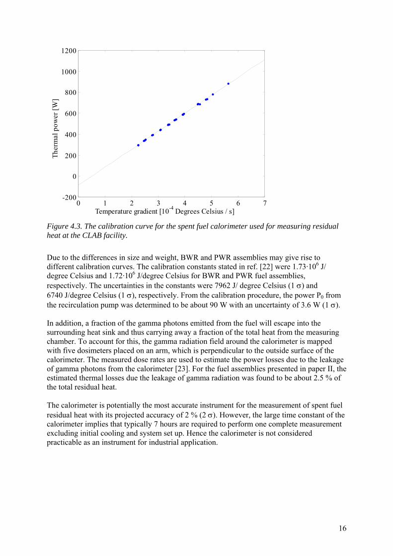
By performing a series of calibration measurements with different power ratings for the heating element, a calibration curve can be constructed to establish a correlation between the thermal power and the rate of temperature rise as defined in eq. 4.2. Figure 4.3 shows the data for a calibration curve as presented in [17, 18].

15

0 1 2 3 4 5 6 7-200

0

200

400

600

800

1000

1200Th

erm

al p

ower

[W]

Temperature gradient [10-4 Degrees Celsius / s] Figure 4.3. The calibration curve for the spent fuel calorimeter used for measuring residual heat at the CLAB facility.

Due to the differences in size and weight, BWR and PWR assemblies may give rise to different calibration curves. The calibration constants stated in ref. [22] were 1.73·106 J/ degree Celsius and 1.72·106 J/degree Celsius for BWR and PWR fuel assemblies, respectively. The uncertainties in the constants were 7962 J/ degree Celsius (1 σ) and 6740 J/degree Celsius (1 σ), respectively. From the calibration procedure, the power P0 from the recirculation pump was determined to be about 90 W with an uncertainty of 3.6 W (1 σ). In addition, a fraction of the gamma photons emitted from the fuel will escape into the surrounding heat sink and thus carrying away a fraction of the total heat from the measuring chamber. To account for this, the gamma radiation field around the calorimeter is mapped with five dosimeters placed on an arm, which is perpendicular to the outside surface of the calorimeter. The measured dose rates are used to estimate the power losses due to the leakage of gamma photons from the calorimeter [23]. For the fuel assemblies presented in paper II, the estimated thermal losses due the leakage of gamma radiation was found to be about 2.5 % of the total residual heat. The calorimeter is potentially the most accurate instrument for the measurement of spent fuel residual heat with its projected accuracy of 2 % (2 σ). However, the large time constant of the calorimeter implies that typically 7 hours are required to perform one complete measurement excluding initial cooling and system set up. Hence the calorimeter is not considered practicable as an instrument for industrial application.

16

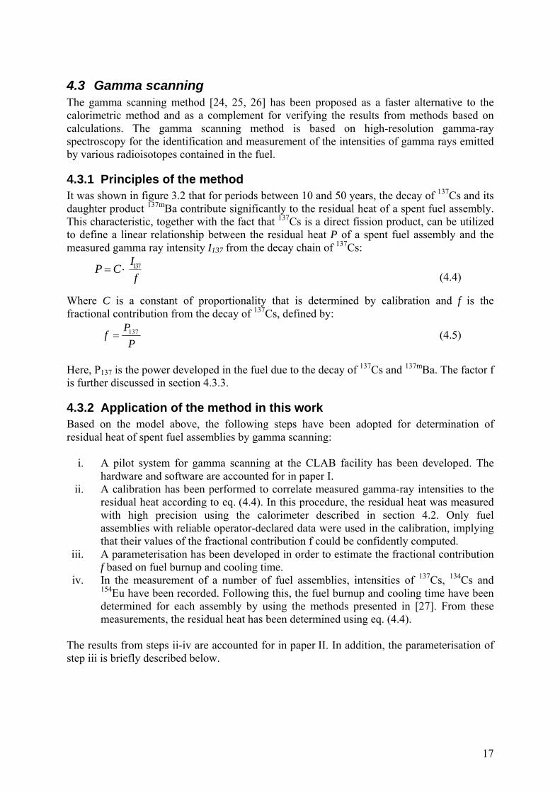
4.3 Gamma scanning The gamma scanning method [24, 25, 26] has been proposed as a faster alternative to the calorimetric method and as a complement for verifying the results from methods based on calculations. The gamma scanning method is based on high-resolution gamma-ray spectroscopy for the identification and measurement of the intensities of gamma rays emitted by various radioisotopes contained in the fuel.

4.3.1 Principles of the method It was shown in figure 3.2 that for periods between 10 and 50 years, the decay of 137Cs and its daughter product 137mBa contribute significantly to the residual heat of a spent fuel assembly. This characteristic, together with the fact that 137Cs is a direct fission product, can be utilized to define a linear relationship between the residual heat P of a spent fuel assembly and the measured gamma ray intensity I137 from the decay chain of 137Cs:

137 IP Cf

= ⋅ (4.4)

Where C is a constant of proportionality that is determined by calibration and f is the fractional contribution from the decay of 137Cs, defined by:

PP

f 137= (4.5)

Here, P137 is the power developed in the fuel due to the decay of 137Cs and 137mBa. The factor f is further discussed in section 4.3.3.

4.3.2 Application of the method in this work Based on the model above, the following steps have been adopted for determination of residual heat of spent fuel assemblies by gamma scanning:

i. A pilot system for gamma scanning at the CLAB facility has been developed. The hardware and software are accounted for in paper I.

ii. A calibration has been performed to correlate measured gamma-ray intensities to the residual heat according to eq. (4.4). In this procedure, the residual heat was measured with high precision using the calorimeter described in section 4.2. Only fuel assemblies with reliable operator-declared data were used in the calibration, implying that their values of the fractional contribution f could be confidently computed.

iii. A parameterisation has been developed in order to estimate the fractional contribution f based on fuel burnup and cooling time.

iv. In the measurement of a number of fuel assemblies, intensities of 137Cs, 134Cs and 154Eu have been recorded. Following this, the fuel burnup and cooling time have been determined for each assembly by using the methods presented in [27]. From these measurements, the residual heat has been determined using eq. (4.4).

The results from steps ii-iv are accounted for in paper II. In addition, the parameterisation of step iii is briefly described below.

17

4.3.3 The fractional contribution, f It has been shown in paper II that for a given cooling time at the time of encapsulation, the fractional contribution f is about linear to the burnup, with a correlation of about -0.4% per GWd/tU. In addition, the exponential decay of the radioactive isotopes motivate, after expansion to the second order in time, a quadratic dependency on cooling time T. Accordingly, the following parameterisation is yielded: f (Bu,T) = A0 + A1Bu + A2(T – T0) + A3(T – T0)2 (4.7) The values of the coefficients A0, A1, A2 and A3 have been determined for the PWR 15x15 and 17x17 fuel types by fitting the values of f obtained from ORIGEN-ARP calculations to burnup and cooling time. In these calculations, the burnup was varied in the interval (15-50) GWd/tU in steps of 3.0 GWd/tU while the cooling time was varied in the interval (15-50) years in steps of 600 days. The enrichment was kept at a constant value of 3 %. The irradiation histories corresponded to regular 5-cycle histories with normal shutdown periods for revision. The results are shown in table 4.1. Fuel geometry A0 A1

[10-3tU/GWd]

A2 [10-3 yrs-1]

A3 [10-5yrs-2]

15x15 17x17

0.415 ± 0.003 0.415 ± 0.003

-1.47 ± 0.06 -1.51 ± 0.06

-1.46± 0.28 -1.47 ± 0.28

-2.07 ± 1.05 -2.12 ± 1.04

Table 4.1. Numerical values of the fitting coefficients An of eq. (2.3). The uncertainty for each coefficient is given (1 σ).

5 Gamma scanning equipment A pilot gamma scanning system has been installed at the CLAB facility in order to investigate the applicability of the technique for experimental determination of residual heat in spent fuel prior to encapsulation. The pilot set-up consists of an elevator system for moving the fuel assembly relative to the detector, a collimator system, a gamma-ray detector, a PC-based multi channel analyser and the data-acquisition and analysis software. The data-acquisition hardware and software are described in paper I.

5.1 The mechanical equipment The mechanical system consists of a fixture that is mounted in the pool wall, a collimator that goes through the pool wall and an elevator. In the fixture, the fuel assembly can be moved vertically in front of the collimator by the elevator system. The arrangement of the fixture allows the fuel assembly to be rotated so that a corner is facing the collimator. A more detailed description of the mechanical equipment is given in [24, 25] while a schematic illustration is shown in figure 5.1.The equipment shown is originally designed for other purposes and is not optimised for the type of measurements reported here.

18

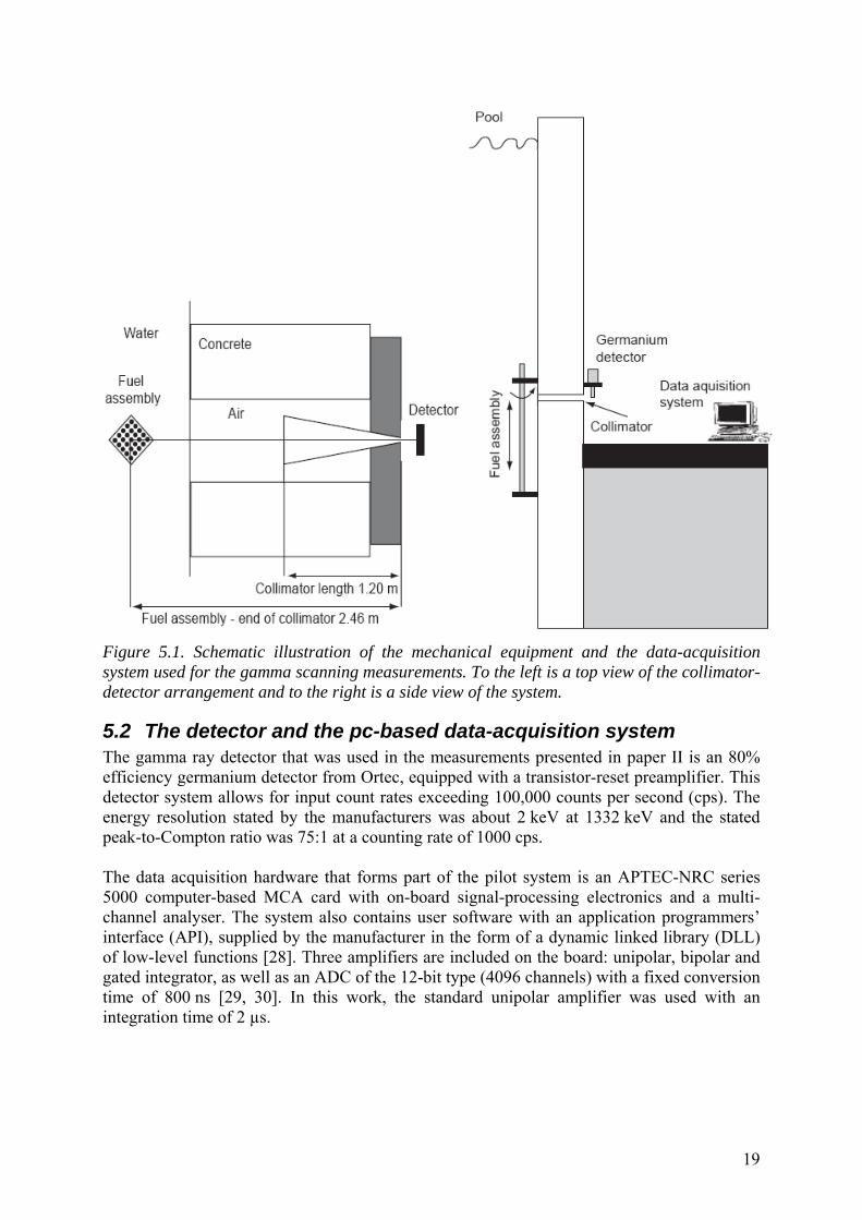
Figure 5.1. Schematic illustration of the mechanical equipment and the data-acquisition system used for the gamma scanning measurements. To the left is a top view of the collimator-detector arrangement and to the right is a side view of the system.

5.2 The detector and the pc-based data-acquisition system The gamma ray detector that was used in the measurements presented in paper II is an 80% efficiency germanium detector from Ortec, equipped with a transistor-reset preamplifier. This detector system allows for input count rates exceeding 100,000 counts per second (cps). The energy resolution stated by the manufacturers was about 2 keV at 1332 keV and the stated peak-to-Compton ratio was 75:1 at a counting rate of 1000 cps. The data acquisition hardware that forms part of the pilot system is an APTEC-NRC series 5000 computer-based MCA card with on-board signal-processing electronics and a multi-channel analyser. The system also contains user software with an application programmers’ interface (API), supplied by the manufacturer in the form of a dynamic linked library (DLL) of low-level functions [28]. Three amplifiers are included on the board: unipolar, bipolar and gated integrator, as well as an ADC of the 12-bit type (4096 channels) with a fixed conversion time of 800 ns [29, 30]. In this work, the standard unipolar amplifier was used with an integration time of 2 µs.

19

5.3 The software As part of the development of the gamma scanning method, data-acquisition and analysis software has been developed. The software packages that were written in the C language have been developed for three main tasks; data acquisition, spectrum analysis and the use of measured gamma-ray intensities for the determination of spent fuel parameters. The main features of the software include:

Modular design, implying that new functionalities can easily be added or changed, Flexibility in the sense that all relevant measuring parameters can be set by the user, Provisions for online- and offline analysis and diagnostics to the user. The user can make

decisions based on the online information.

5.3.1 The data-acquisition software The data-acquisition software package was developed specifically for the acquisition and storage of gamma-ray spectra during the scan of a fuel assembly. It has a modular design for easy adaptation to changes in hardware. In the case of the series-5004 MCArd, the low-level functions are called from the MCArd DLL. The calls to the low-level functions allow the data-acquisition software to perform the following tasks: Detect and initialise the acquisition hardware. Send and receive control data from the hardware, including for example the number of

ADC channels to be used for spectrum collection, the type of amplifier and the integration time of the amplifier.

Start and stop spectrum collection. Receive acquired spectrum and spectrum collection information.

In addition to the control of the data-acquisition hardware, the software also performs some of the basic functions of an MCA emulator.

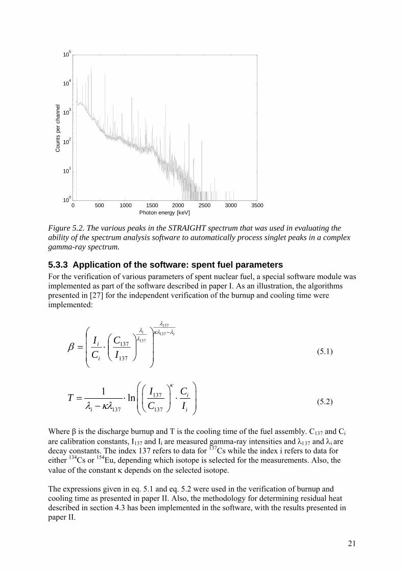
5.3.2 The spectrum analysis software The spectrum analysis package can perform automatic and repetitive analysis of collected gamma-ray spectra. In this regard, the software is able to perform peak width calibration, automatic peak search and identification, determination of peak boundaries, background subtraction, determination of peak area and decomposition of peak doublets. In particular, the spectrum-analysis software calculates and presents the axial distributions of the relative isotopic intensities of the radioisotopes: 154Eu, 137Cs, 60Co and 134Cs. The measured intensities of these isotopes are then applied by the software in the determination/verification of spent fuel parameters such as cooling time, discharge burnup and residual heat, as described in section 5.3.3. The algorithms used have been tested and evaluated using the 1995 test spectra from the IAEA [31] and the Sanderson collection of test spectra [32]. Figure 5.2 shows the peaks in the “STRAIGHT” spectrum from the IAEA collection. This is a plain 226Ra spectrum that was collected for 2000 seconds real time, containing more than 150 peaks of varying intensities. The results of the evaluation were considered to be satisfying, demonstrating the applicability of the software for complex gamma-ray spectra. This is further discussed in paper I. In addition to these tests, the software has been used in gamma-scanning measurements at the interim storage for spent nuclear fuel (CLAB) in Oskarshamn, Sweden. Details and results of these measurements are presented in paper II.

20

0 500 1000 1500 2000 2500 3000 3500100

101

102

103

104

105

Cou

nts

per c

hann

el

Photon energy [keV] Figure 5.2. The various peaks in the STRAIGHT spectrum that was used in evaluating the ability of the spectrum analysis software to automatically process singlet peaks in a complex gamma-ray spectrum.

5.3.3 Application of the software: spent fuel parameters For the verification of various parameters of spent nuclear fuel, a special software module was implemented as part of the software described in paper I. As an illustration, the algorithms presented in [27] for the independent verification of the burnup and cooling time were implemented:

ii

IC

CI

i

i

λκλλ

λλ

β−

⎟⎟⎟

⎠

⎞

⎜⎜⎜

⎝

⎛

⎟⎟⎠

⎞⎜⎜⎝

⎛⋅=

137

137

137

137

137 (5.1)

137

137 137

1 ln i

i i

I CTC I

κ

λ κλ

⎛ ⎞⎛ ⎞⎜= ⋅ ⋅⎜ ⎟⎜− ⎝ ⎠⎝ ⎠

⎟⎟ (5.2)

Where β is the discharge burnup and T is the cooling time of the fuel assembly. C137 and Ci

are calibration constants, I137 and Ii are measured gamma-ray intensities and λ137 and λi are decay constants. The index 137 refers to data for 137Cs while the index i refers to data for either 134Cs or 154Eu, depending which isotope is selected for the measurements. Also, the value of the constant κ depends on the selected isotope. The expressions given in eq. 5.1 and eq. 5.2 were used in the verification of burnup and cooling time as presented in paper II. Also, the methodology for determining residual heat described in section 4.3 has been implemented in the software, with the results presented in paper II.

21

6 Experimental studies Paper II accounts for an experimental study of 31 spent PWR fuel assemblies using the gamma scanning method and the pilot system described in paper I. The major goals of the measurements were to perform a calibration of the pilot gamma-scanning system based on measurements of spent fuel residual heat using the calorimeter described in section 4.2 and to demonstrate the attainable accuracy of the gamma-scanning technique.

The application of the gamma scanning measurements was divided into two cases of interest for the encapsulation plant:

(i) Spent fuel discharge data is considered to be available, thereby making the gamma-scanning measurements a verification of the calculated residual heat, and

(ii) Cases where no data about the fuel assemblies is available except for knowledge of the assembly type, making the gamma-scanning measurements a stand-alone determination of the residual heat.

These two cases are further discussed in section 6.4 and 6.5, respectively. A more detailed account for the results can be found in paper II.

6.1 Overview of the measurement procedure The measurement procedure is described in more detail in [25] and only the basic features are presented here. A measurement is performed by scanning all four corners of the fuel assembly axially. Each corner takes about 3-4 minutes implying a total measuring time of 15 minutes. During each scan, data (sub-spectra) are registered for typically one second and then transferred from the ADC memory to the computer. Typically, a few hundred sub-spectra are collected per corner so that gamma-ray intensities are registered along the whole fuel length. The collected sub-spectra can be treated in a number of ways depending on the specific task, e.g. added to yield spectra corresponding to each axial node of the fuel assembly or summed to form a total spectrum.

6.2 Calibration and normalization To obtain the proportionality constant C in eq. (4.4), a calibration procedure was performed. The first step in the calibration was to identify a number of fuel assemblies that were considered to be “normal” in every aspect, here called reference assemblies. In this context, normal means that no reconstruction of the assemblies has taken place and that the irradiation histories are consistent with regular reactor operation. Since the constant C depends on the measurement geometry and the fuel type, the calibration was performed separately for the 15x15 and 17x17 fuel assemblies reported in paper II. In the calibration procedure, the measured 137Cs gamma-ray intensities for the reference assemblies were corrected for the fractional contribution f as described in section 4.3, and for the decay period between the calorimetric measurements and the gamma scanning measurements. By using a linear least square procedure to fit the corrected intensities to the residual heat from the calorimetric measurements, the calibration constant was obtained for the two fuel types reported.

22

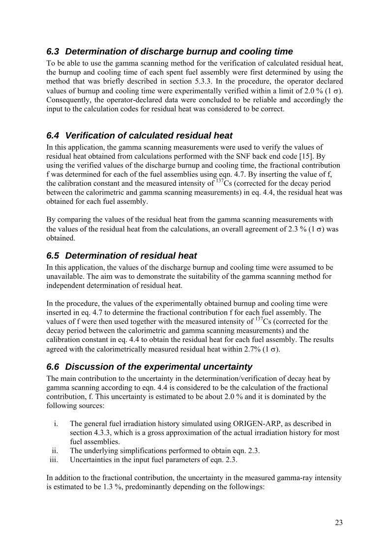
6.3 Determination of discharge burnup and cooling time To be able to use the gamma scanning method for the verification of calculated residual heat, the burnup and cooling time of each spent fuel assembly were first determined by using the method that was briefly described in section 5.3.3. In the procedure, the operator declared values of burnup and cooling time were experimentally verified within a limit of 2.0 % (1 σ). Consequently, the operator-declared data were concluded to be reliable and accordingly the input to the calculation codes for residual heat was considered to be correct.

6.4 Verification of calculated residual heat In this application, the gamma scanning measurements were used to verify the values of residual heat obtained from calculations performed with the SNF back end code [15]. By using the verified values of the discharge burnup and cooling time, the fractional contribution f was determined for each of the fuel assemblies using eqn. 4.7. By inserting the value of f, the calibration constant and the measured intensity of 137Cs (corrected for the decay period between the calorimetric and gamma scanning measurements) in eq. 4.4, the residual heat was obtained for each fuel assembly. By comparing the values of the residual heat from the gamma scanning measurements with the values of the residual heat from the calculations, an overall agreement of 2.3 % (1 σ) was obtained.

6.5 Determination of residual heat In this application, the values of the discharge burnup and cooling time were assumed to be unavailable. The aim was to demonstrate the suitability of the gamma scanning method for independent determination of residual heat. In the procedure, the values of the experimentally obtained burnup and cooling time were inserted in eq. 4.7 to determine the fractional contribution f for each fuel assembly. The values of f were then used together with the measured intensity of 137Cs (corrected for the decay period between the calorimetric and gamma scanning measurements) and the calibration constant in eq. 4.4 to obtain the residual heat for each fuel assembly. The results agreed with the calorimetrically measured residual heat within 2.7% (1 σ).

6.6 Discussion of the experimental uncertainty The main contribution to the uncertainty in the determination/verification of decay heat by gamma scanning according to eqn. 4.4 is considered to be the calculation of the fractional contribution, f. This uncertainty is estimated to be about 2.0 % and it is dominated by the following sources:

i. The general fuel irradiation history simulated using ORIGEN-ARP, as described in section 4.3.3, which is a gross approximation of the actual irradiation history for most fuel assemblies.

ii. The underlying simplifications performed to obtain eqn. 2.3. iii. Uncertainties in the input fuel parameters of eqn. 2.3.

In addition to the fractional contribution, the uncertainty in the measured gamma-ray intensity is estimated to be 1.3 %, predominantly depending on the followings:

23

i. The accuracy of the positioning of the fuel assembly in the mechanical arrangement, which directly affects the accuracy of the determination of the intensity from 137Cs.

ii. The uncertainties of the dead-time correction factors applied for each subspectrum. Finally, the uncertainty in the fitting constant C of eq. 4.4 is estimated to be below 0.5 %, as accounted for in table IV of paper II. Based on the above contributions, the accuracy of the gamma scanning method presented in this work can be estimated to be about 2.5 %. This value is in agreement with the results presented in table VI and table VII of paper II.

7 Conclusions and outlook The activities reported in this thesis are part of a project aimed at the development of an integrated measurement system for the characterization of spent nuclear fuel assemblies at the proposed spent fuel encapsulation plant in Sweden. As part of the activities, data-acquisition and analysis software for a pilot gamma scanning system has been developed. The system was tested for measurements at the CLAB facility and the results obtained demonstrated the suitability of the gamma scanning method for this application. However, the pilot system was based on equipment that was already available at CLAB. It is anticipated that the experiences gained with this system will be incorporated into the design of a more advanced system for application at the encapsulation plant. Furthermore, only PWR fuel assemblies were accounted for in paper II. Since there are 7 BWR and 3 PWR plants in operation in Sweden, more efforts have to be put in evaluating the gamma-scanning technique also for BWR fuel. Accordingly, more gamma scanning measurements as well as SNF calculations and calorimetric measurements will be performed during 2007 to account also for the BWR fuel types. Sequel to the discussion in section 2.1 on fuel types, very little consideration was given to reconstructed fuel assemblies due to the fact that the reconstruction of a fuel assembly changes its geometry, which in turn affects the calibration constant in eq. 4.4. Correction factors will be needed in order to be able to apply the calibration and normalization procedures for the determination of the residual heat for such fuel assemblies. Therefore, when information is available about the reconstruction of a fuel assembly, a possible strategy will be the use of gamma ray transport coefficients, as calculated with a technique used in tomographic computations [33]. This strategy will allow the calibration constants C for different fuel designs and geometries to be related to each other for the following cases:

a) Fuel designs that have not been calibrated. b) Reconstructed fuel assemblies where fuel rods have been removed or replaced. c) PWR fuel assemblies that contains control rods clusters.

The application of the strategy requires that reliable information about the current fuel geometry is available. For cases where this information is questionable, the use of the tomographic measurements could provide a means of verifying the current geometry of the fuel assemblies. In addition, the procedure described in section 4.3 for determining the value of f for a fuel assembly assumes a regular irradiation history. However, the inventory of spent fuel assemblies at the CLAB facility includes fuel assemblies that have irregular irradiation history such as several-year outages between core resident periods. The out-of-core periods in the

24

irradiation history result in a decrease in the contribution of short-lived radioisotopes to the residual heat. For these classes of fuel assemblies, alternative modelling of the fractional contribution may be required. This subject is also discussed in paper II.

8 Acknowledgements I am grateful for the financial support given by the Swedish Nuclear Fuel Management Company, SKB and the Graduate School for Advanced Instrumentation and Measurements (AIM). In addition, I wish to thank my supervisors Ane Håkansson, Staffan Jacobsson Svärd and Anders Bäcklin for their support and contributions to this work among other things, members of my research group: Klaes-Håkan Bejmer, Christopher Willman, Anni Fritzell, Tobias Lundqvist, Charlotte Lager and Karen Kvenangen, members of the project group for spent fuel residual heat: Anders Nyström at SKB, Per Grahn at SKB International, Tomas Rosengren at SKB, Lennart Agrenius at Agrenius ingenjörsbyrå, Fredrik Sturek at OKG and Fredrik Aronsson at OKG, Staff and Graduate Students at the Department of Neutron Research and the Department of Nuclear and Particle Physics.

References 1 NEI, World Nuclear Power Generation and Capacity, Web address:

http://www.nei.org/documents/world_nuclear_generation_and_capacity.pdf, January 09, 2007.

2 NEA, Nuclear Energy Today (2003), Website: http://www.nea.fr/html/pub/nuclearenergytoday/welcome.html, December 01, 2006.

3 Nuclear Energy Agency (NEA), Trends in the Nuclear Fuel Cycle: Economic, Environmental and Social Aspects (2002).

4 B. ROUBEN, Introduction to Reactor Physics, Reactor Core Physics Branch, Atomic Energy of Canada Ltd (AECL), (2002), web address: http://canteach.candu.org/library/20040501.pdf, January 09, 2007.

5 KSU, Reaktorfysik, Introductory course material in Reactor Physics (in Swedish). 6 R. HEIKKI, Disposal Canister for Spent Nuclear Fuel-Design Report, POSIVA 2005-02

(2005). 7 R. HEIKKI, Thermal Dimensioning of Repository and Its Influence on Operation Time-

Scale, POSIVA TS-M-18/04 (2004). 8 P. AHLSTRÖM, Nuclear Engineering and Design, 176 (1997) 67. 9 L. AGRENIUS, Criticality safety calculations of storage canisters, SKB report: TR-02-

17, (2002). 10 IAEA, Operation of Spent Fuel Storage Facilities, Safety Series No 117 (1994). 11 M. P. STAHALA, High level nuclear waste repository thermal loading analysis,

Master’s Thesis, North Carolina State University, (2006). 12 M. C MALBRAIN, Analytical characterization of spent fuels and high level wastes and

application to the thermal designs of a geological repository in salt, Master’s Thesis, Massachusetts Institute of Technology, (1981).

13 B. DUCHEMIN, C. NORDBORG, “Decay Heat Calculation, An International Nuclear Code Comparison”, NEACRP-319, Nuclear Energy Agency, (1989). Retrieved from: http://www.nea.fr/html/science/docs/1989, January 15, 2007.

14 I. C. GAULD, “Decay Heat Code Validation Activities at ORNL: Supporting Expansion of NRC Regulatory Guide 3.54”, ANS winter meeting (2001). Retrieved from: http://www.ornl.gov/~webworks/cppr/y2001/pres/111200.pdf, January 27, 2007.

15 S. BØRRESEN and M. KRUNERS, Validation of SNF against CLAB decay heat measurements, SSP-04/216, Studsvik Scandpower (2005).

25

16 S. BØRRESEN, private communication. 17 F. STUREK, L. AGRENIUS, CLAB - Measurements of decay heat in spent fuel

assemblies, SKB draft report (2005). 18 F. STUREK, CLAB - Kalibreringkurva för kalorimetrisk mätning av bränsleelement

OKG draft report (2003) (Swedish). 19 S. R. GUNN, “Radiometric Calorimetry: a Review,” Nucl. Instrum. Meth,. 29, 1 (1964). 20 H. RAMTHUN, “Recent Developments in Calorimetric Measurements of

Radioactivity,” Nucl. Instrum. Meth., 112, 265 (1973). 21 W. ZIELENKIEWICZ, E. MARGAS, Theory of Calorimetry, Kluwer Academic

Publishers, 2004. 22 L. AGRENIUS, CLAB -Uncertainty analysis of the calorimeter (system 251) using the

temperature increase method, draft 2 / 2004-03-25 (2004). 23 A. HÅKANSSON, O. OSIFO, Rapport angående avgiven gammaeffekt i BWR- och

PWR-bränsle, SKB draft report 2004 (in Swedish). 24 P. JANSSON, A. HÅKANSSON, A. BÄCKLIN and S. JACOBSSON, Gamma-ray

Spectroscopy Measurements of Decay Heat in Spent Nuclear Fuel, Nuclear Science and Engineering ,141, 129 (2002).

25 P. JANSSON, Studies of Nuclear Fuel by Means of Nuclear Spectroscopic Methods, Acta Universitates Upsaliensis, (Uppsala 2002), PhD Dissertation, Uppsala University, Uppsala, Sweden.

26 A. HÅKANSSON, A. BÄCKLIN, Project report, Department of Radiation Sciences, Uppsala University, Uppsala, TSL/ISV-95-0121, IISN 0284 - 2769, May 1995.

27 C. WILLMAN, A. HÅKANSSON, O. OSIFO, A. BÄCKLIN and S. JACOBSSON SVÄRD, Non-destructive assay of Spent Nuclear Fuel with Gamma-Ray Spectroscopy, Annals of Nuclear Energy, 33, 427 (2006).

28 APTEC-NRC, PCMCA/Super, Basic Display and Acquisition Software, Rev. 00. 29 APTEC-NRC, Detailed Software and Board Documentation, Rev. 07. 30 APTEC-NRC, PC BASED MCA CARDS For No-NIMS Spectroscopy. 31 IAEA, Intercomparison of gamma-ray analysis software packages, IAEA-TECDOC-

1011, Vienna IAEA, (1998). 32 K. M. DECKER, C. G. SANDERSON, A re-evaluation of commercial IBM PC

software for the analysis of low level environmental gamma-ray spectra, Appl. Radiat. Isot. 43 (1992) 323.

33 S. JACOBSSON SVÄRD, A Tomographic Measurement Technique for Irradiated Nuclear Fuel Assemblies, PhD Thesis, Uppsala University (2004).

26

Data acquisition and analysis software for rapid gamma scanning: application for the verification of spent LWR fuel parameters Otasowie Osifo, Ane Håkansson, Staffan Jacobsson Svärd, Anders Bäcklin Department of Neutron Research, Uppsala University, Sweden

Abstract A pilot gamma scanning system is being developed as part of the research and development program for the planned spent nuclear fuel encapsulation plant in Sweden. For this system, a software package has been developed with modules for fast automatic repetition of spectrum acquisition and consecutive spectrum analysis. The software is also able to interact with a database of fuel information, including operator-declared data and measured data. The software package has been used in the gamma scanning of spent PWR fuel assemblies at the interim storage facility for spent nuclear fuel (CLAB) in Oskarshamn, Sweden. Results obtained from the measurements are presented. The analyses show that fuel burnup, cooling time and residual heat can be verified within 2-3 % (1 σ).

1 Introduction and background The Swedish strategy for nuclear fuel management is based on a once through principle, implying that no part of the spent fuel will be recycled. Instead, the strategy envisions the encapsulation of the spent fuel assemblies in copper canisters that will be embedded in bentonite clay in a deep underground repository. Each canister is expected to contain about twelve BWR or four PWR fuel assemblies [1]. In connection with the encapsulation plant, the Swedish Nuclear Fuel and Waste Management Company (SKB) is planning a measurement station for the verification and determination of spent fuel parameters. The parameters of interest include decay heat, fuel discharge burnup and cooling time [2, 3]. For this purpose, the gamma scanning method will be used implying fast repetitive measurements of gamma-ray spectra. This paper describes the software developed for data acquisition and analysis. The algorithms in the software have been tested and evaluated by using the 1995 test spectra from the IAEA [4, 5, 6] and the Sanderson collection of test spectra [7]. In addition to these tests, the software has been used in gamma-scanning measurements at the interim storage for spent nuclear fuel (CLAB) in Oskarshamn, Sweden [8].

2 Overview of the gamma scanning method As shown in [2, 3], the gamma scanning method is suited for the verification of spent fuel parameters such as burnup, cooling time, decay heat and nodal burnup profile analysis. It is based on high-resolution gamma-ray spectroscopy that is used to measure the intensities of gamma rays emitted by various radioisotopes contained in the spent fuel. The important radioisotopes include: 137Cs (T1/2 = 30y), 134Cs (T1/2 = 2.1y) and 154Eu (T1/2 = 8.6y) with principal gamma-ray energies of 662 keV, 795 keV and 1275 keV, respectively. The method relies on calibration and normalization procedures in order to relate the measured gamma-ray

1

intensities to the relevant spent fuel parameters. Details of such calibration and normalization procedures are described in [2, 3, 9]. The pilot set-up consists of an elevator system for moving the fuel element relative to the detector, a collimator system, an 80 % efficiency germanium detector, a pc-based multichannel analyzer and the software described here. The measurement procedure has been described in detail in [2, 3, 9] and only the basic features that includes the axial scan of each of the four corners of a fuel assembly are described here. During each scan, data (sub-spectra) are registered for typically one second and then transferred from the ADC memory to the computer. Typically, a few hundred sub-spectra are collected per corner so that gamma-ray intensities are registered along the whole fuel length. The collected sub-spectra can be treated in a number of ways depending on the specific task, e.g. added to yield spectra corresponding to each axial node of the fuel assembly or summed to form a total spectrum. The steps contained in the gamma scanning procedure demand that the gamma scanning software fulfils certain design requirements that are specific to the operational goals of the encapsulation plant. Accordingly, the software has been designed to fulfil the following requirements:

• The time used for data taking and analysis of the data should only be a small fraction of the total handling time allocated for each fuel assembly.

• The data-acquisition software should allow for measuring a preset number of sub-spectra each lasting a preset period of time.

• The analysis software shall compute average and nodal intensities and associated uncertainties of selected isotopes for each of the four corners of a fuel assembly.

• The analysis software shall contain the calibration and normalization procedure necessary for verification of decay heat, discharge burnup and cooling time.

• The software should be built in modular form in order to ensure flexibility.

3 The data-acquisition system

3.1 Hardware Figure 3.1 shows a block diagram of the system. For the current application, a high-resolution germanium detector is used and because high-intensity gamma radiation was expected in conjunction with low-intensity radiation, the detector had to be able to record events at count rates of up to 105 cps in order to reach sufficient statistics while minimizing the measuring time. For the pilot system, an 80 % efficiency germanium detector equipped with a transistor-reset preamplifier was selected. It allows for input count rates exceeding 100,000 counts per second (cps) with an energy resolution of about 2 keV at 1332 keV. The MCA is part of a plug-in-PC board from APTEC-NRC [10, 11], which is a fully decoded data-acquisition card that can be plugged into one of the ISA slots on a personal computer. The board contains three types of pulse shaping amplifiers: unipolar, bipolar and gated integrator with shaping time constants ranging from 0.25 μs to 8.0 μs. The onboard ADC has a resolution of 12 bits (4096 channels) with a fixed conversion time of 800 ns and it can store integer values up to 232 – 1 per channel. The card is used to perform such tasks as detector

2

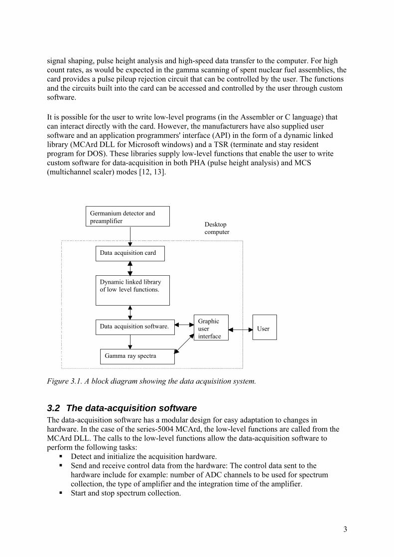
signal shaping, pulse height analysis and high-speed data transfer to the computer. For high count rates, as would be expected in the gamma scanning of spent nuclear fuel assemblies, the card provides a pulse pileup rejection circuit that can be controlled by the user. The functions and the circuits built into the card can be accessed and controlled by the user through custom software. It is possible for the user to write low-level programs (in the Assembler or C language) that can interact directly with the card. However, the manufacturers have also supplied user software and an application programmers' interface (API) in the form of a dynamic linked library (MCArd DLL for Microsoft windows) and a TSR (terminate and stay resident program for DOS). These libraries supply low-level functions that enable the user to write custom software for data-acquisition in both PHA (pulse height analysis) and MCS (multichannel scaler) modes [12, 13].

Germanium detector and preamplifier

Data acquisition card

Dynamic link ed library of low level functions.

Data acquisition software.Graphic userinterface

User

Gamma ray spectra

Desktop computer

Figure 3.1. A block diagram showing the data acquisition system.

3.2 The data-acquisition software The data-acquisition software has a modular design for easy adaptation to changes in hardware. In the case of the series-5004 MCArd, the low-level functions are called from the MCArd DLL. The calls to the low-level functions allow the data-acquisition software to perform the following tasks: Detect and initialize the acquisition hardware. Send and receive control data from the hardware: The control data sent to the

hardware include for example: number of ADC channels to be used for spectrum collection, the type of amplifier and the integration time of the amplifier.

Start and stop spectrum collection.

3

Receive acquired spectrum and spectrum collection information. In addition to the control of the data-acquisition hardware, the software also performs some of the basic functions of an MCA emulator. These include energy calibration of the ADC, spectrum display, simple peak location and peak area measurements for selected radioisotopes. The modules that combine to make up the acquisition software are described below.

3.2.1 The graphic user interface (GUI) The GUI allows the user to interact with the data-acquisition software and hardware through various display options. The tasks performed with the GUI include the display of collected spectra and acceptance of the following user supplied inputs:

• Choice of MCArd from a list. • Type of preamplifier. • Choice of amplifier from a list. • Setting of amplifier shaping time from a list. • Number of ADC channels. • Setting parameters for pulse pileup rejection. • Setting for the discriminator level of the amplifier • Setting for the discriminator levels of the ADC. • The number of times the ADC memory is accessed while scanning a fuel assembly

along its axis i.e. the number of sub-spectra. • The data collection time for each sub-spectrum.

3.2.2 The initialisation module The initialisation module is used to detect and initialise the MCArd for spectrum collection. It uses the settings defined by the user in the GUI. The initialisation is done through the functions provided by the MCArd DLL while the data-acquisition software provides functions such as energy calibration and peak width calibration for the automatic peak search routine for usage during initialisation. Although the initialisation module presently uses only the MCArd DLL, it is possible to extend this ability to include initialisation of other data-acquisition cards by adding calls to the low-level functions provided for such cards.

3.2.3 The data-acquisition module The data-acquisition module is used to start and stop the spectrum collection in each scan of a fuel assembly. It is also used to access the ADC memory while performing a scan. Each access to the ADC memory collects a spectrum at the user-defined interval along the axial length of the fuel. The module uses the low-level functions provided in the MCArd DLL. The data from each access to the ADC memory is stored in a matrix in the memory of the computer while the fuel assembly is being scanned. When an axial scan is completed, the acquired spectra and pertinent data such as live time, true time, number of ADC channels, energy calibration etc are transferred from the process memory to the hard disk. The storage format for the data files is the ASCII (.asc) format. However, it is possible to add new routines to the software in order to enable it to read, write and display spectrum files which adhere e.g. to the vendor neutral ANSI N42.42 data file format [14]. In addition, the

4

data-acquisition module can be expanded to use calls to low-level functions for spectrum collection provided by other types of plug-in-cards.

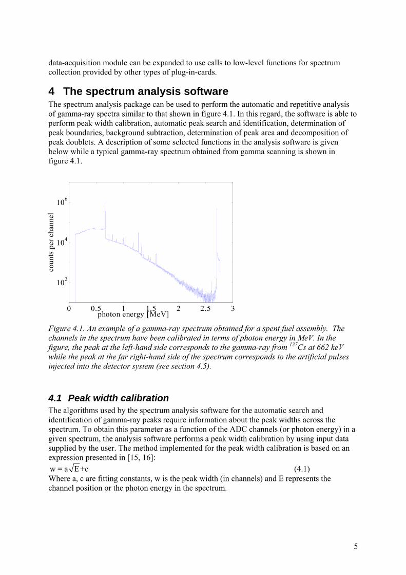
4 The spectrum analysis software The spectrum analysis package can be used to perform the automatic and repetitive analysis of gamma-ray spectra similar to that shown in figure 4.1. In this regard, the software is able to perform peak width calibration, automatic peak search and identification, determination of peak boundaries, background subtraction, determination of peak area and decomposition of peak doublets. A description of some selected functions in the analysis software is given below while a typical gamma-ray spectrum obtained from gamma scanning is shown in figure 4.1.

0 0.5 1 1.5 2 2.5 3

102

104

106

photon energy [MeV]

coun

ts p

er c

hann

el

Figure 4.1. An example of a gamma-ray spectrum obtained for a spent fuel assembly. The channels in the spectrum have been calibrated in terms of photon energy in MeV. In the figure, the peak at the left-hand side corresponds to the gamma-ray from 137Cs at 662 keV while the peak at the far right-hand side of the spectrum corresponds to the artificial pulses injected into the detector system (see section 4.5).

4.1 Peak width calibration The algorithms used by the spectrum analysis software for the automatic search and identification of gamma-ray peaks require information about the peak widths across the spectrum. To obtain this parameter as a function of the ADC channels (or photon energy) in a given spectrum, the analysis software performs a peak width calibration by using input data supplied by the user. The method implemented for the peak width calibration is based on an expression presented in [15, 16]: w = a E +c (4.1) Where a, c are fitting constants, w is the peak width (in channels) and E represents the channel position or the photon energy in the spectrum.

5

4.2 Automatic identification of gamma ray peaks Automatic peak search and identification is a feature that is useful in the batch processing of a large number of gamma-ray spectra. The implemented algorithm for automatic peak search is based on a variation of the gamma-ray spectrum filter that was described in [17]. In the method, the filter is scanned across the original spectrum, resulting in a spectrum with reduced background continuum and reduced statistical fluctuations. By setting a threshold, peaks can be located in the filtered spectrum and associated with potential photo peaks in the original gamma-ray spectrum. The centroid of each potential photo peak that was identified by the peak search routine was then calculated by the moment method as described in [18]. To be able to identify the gamma ray peaks found by the search algorithm, an energy matching procedure is applied. In the procedure, information supplied by the user, the energy calibration of the spectrum and the results of the peak search, are used. The peak information supplied by the user are matched to the detected photo peaks according to the following criterion:

0- 0E dE m x E E dp ≤ ⋅ + ≤ + Ep (4.2)

Where Ep is the expected energy of the gamma ray peak selected by the user and x0 is the centroid measured in channels for the potential peaks identified by the peak search routine. The parameter m is the spectrum channel width, E0 is the energy offset of the ADC and dE is the inferred energy matching sensitivity, which is estimated from:

2 2 2 2 20 0 m xdE = ΔE + σ + x σ + m σ (4.3)

Here σ0, σm and σx are the estimated uncertainties in the parameters E0, m and x0 respectively. ΔE is a user-defined variable that allows for a peak shift of a few channels.

4.3 Definition of the photopeak region Once a peak has been identified, its low-energy and high-energy boundaries are defined. These boundaries are set at 2 FWHM and 1.5 FWHM from the peak centroid, respectively [19]. Here, the value of FWHM is obtained from the peak width calibration as described in section 4.1. This method ensures that the number of channels in the region of interest for the peak is defined independently of the number of counts in the peak. However, it is also possible for the user to override the automatic definitions and define the peak region of interest manually. This allows the user to take the properties of the particular spectrum into consideration before defining the peak boundaries.

4.4 Background subtraction When the lower and upper boundaries of the peak have been defined as described in section 4.3, background regions are defined starting at a channel distance of typically 3 FWHM on either side of the peak centroid. The default number of channels used for each background region was set to 2 FWHM. However, the number of channels used in the background regions should be determined from an initial examination of the regions about a peak centroid in order not to include other gamma-ray peaks. The background regions are then used to define the background counts to be subtracted from the gross counts in the peak [20, 21, 22]. The background may also be described as a linear background or as a step function as described here:

6

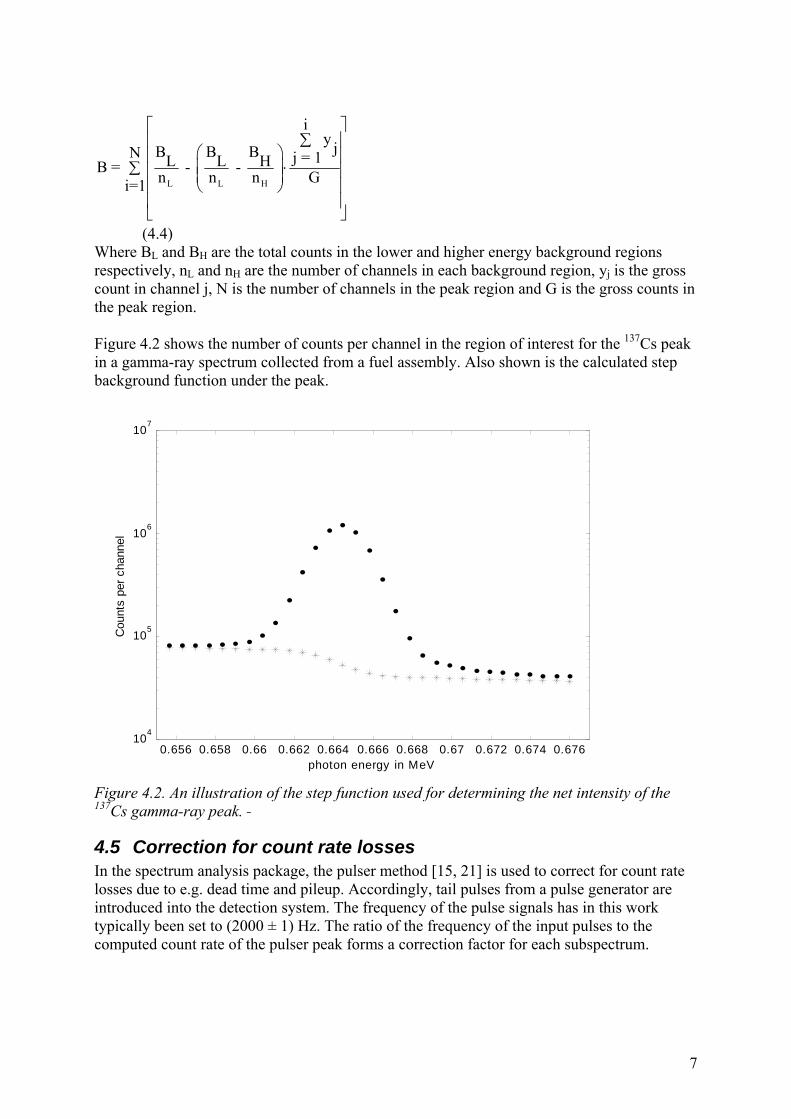
L L H

iy jB B BN j = 1L L HB = - - n n n Gi=1

⎡ ⎤∑⎢ ⎥

⎛ ⎞⎢⋅⎜ ⎟∑ ⎢ ⎜ ⎟

⎝ ⎠⎢ ⎥⎢ ⎥⎣ ⎦

⎥⎥

(4.4) Where BL and BH are the total counts in the lower and higher energy background regions respectively, nL and nH are the number of channels in each background region, yj is the gross count in channel j, N is the number of channels in the peak region and G is the gross counts in the peak region. Figure 4.2 shows the number of counts per channel in the region of interest for the 137Cs peak in a gamma-ray spectrum collected from a fuel assembly. Also shown is the calculated step background function under the peak.

0.656 0.658 0.66 0.662 0.664 0.666 0.668 0.67 0.672 0.674 0.676104

105

106

107

photon energy in MeV

Cou

nts

per c

hann

el

Figure 4.2. An illustration of the step function used for determining the net intensity of the 137Cs gamma-ray peak.

4.5 Correction for count rate losses In the spectrum analysis package, the pulser method [15, 21] is used to correct for count rate losses due to e.g. dead time and pileup. Accordingly, tail pulses from a pulse generator are introduced into the detection system. The frequency of the pulse signals has in this work typically been set to (2000 ± 1) Hz. The ratio of the frequency of the input pulses to the computed count rate of the pulser peak forms a correction factor for each subspectrum.

7

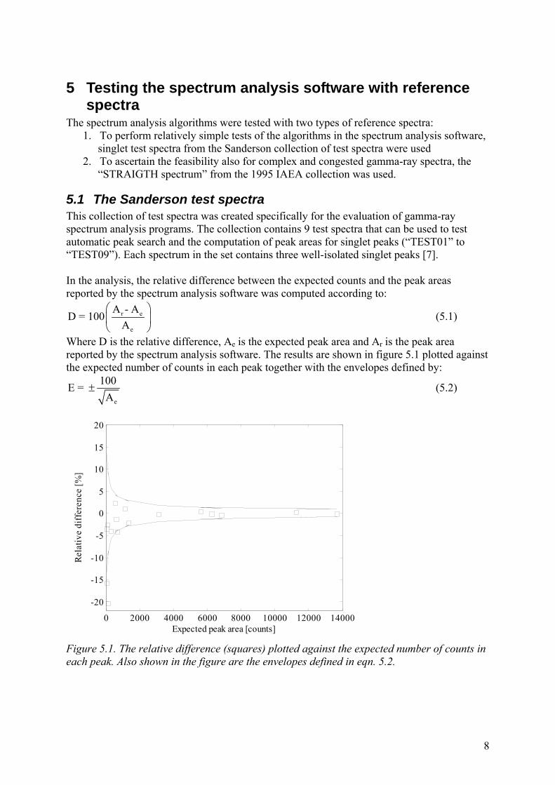
5 Testing the spectrum analysis software with reference spectra

The spectrum analysis algorithms were tested with two types of reference spectra: 1. To perform relatively simple tests of the algorithms in the spectrum analysis software,

singlet test spectra from the Sanderson collection of test spectra were used 2. To ascertain the feasibility also for complex and congested gamma-ray spectra, the

“STRAIGTH spectrum” from the 1995 IAEA collection was used.

5.1 The Sanderson test spectra This collection of test spectra was created specifically for the evaluation of gamma-ray spectrum analysis programs. The collection contains 9 test spectra that can be used to test automatic peak search and the computation of peak areas for singlet peaks (“TEST01” to “TEST09”). Each spectrum in the set contains three well-isolated singlet peaks [7]. In the analysis, the relative difference between the expected counts and the peak areas reported by the spectrum analysis software was computed according to:

r e

e

A - AD = 100A

⎛ ⎞⎜⎝ ⎠

⎟ (5.1)

Where D is the relative difference, Ae is the expected peak area and Ar is the peak area reported by the spectrum analysis software. The results are shown in figure 5.1 plotted against the expected number of counts in each peak together with the envelopes defined by:

e

100E = A

± (5.2)

0 2000 4000 6000 8000 10000 12000 14000

-20

-15

-10

-5

0

5

10

15

20

Expected peak area [counts]

Rela

tive

diff

eren

ce [%

]

Figure 5.1. The relative difference (squares) plotted against the expected number of counts in each peak. Also shown in the figure are the envelopes defined in eqn. 5.2.

8

As shown in figure 5.1, the spectrum analysis software reported good results for peaks with good statistics. For the peaks with the smallest area (less than 65 counts), the relative differences were somewhat larger, with a systematic tendency to underestimate the peak area.

5.2 The 1995 IAEA test spectra This collection of reference spectra is described in [4, 5, 6] and it contains spectra for evaluating gamma-ray spectroscopic software in terms of doublet resolution, peak area and peak area uncertainty determination, efficiency and peak shape calibrations. The simplest spectrum in the collection is the “STRAIGHT” spectrum, which is a plain 226Ra spectrum that was collected for 2000 seconds real time. In the test procedure, 43 peaks with emission probabilities greater than 0.1 % [23, 24] and classified as singlets in [24] were selected for automatic analysis through the energy matching method discussed in Section 4.2. For each of the peaks detected by the peak search algorithm, a measure of the statistical control of the spectrum analysis software was computed from the standardized residuals defined as [6]:

rep refrep 2 2

rep ref

A - AZ =

σ + σ

Where Zrep is the reported standardized residual for the peak, Arep is the peak area reported by the spectrum analysis software, Aref is the reference peak area reported by the IAEA, σrep is the uncertainty in the peak area reported by the spectrum analysis software, and σref is the reference uncertainty in the peak area reported by the IAEA. The values of Zrep for the selected peaks are presented in the histogram shown in figure 5.2.

-3 -2 -1 0 1 20

1

2

3

4

5

6

7

8

Freq

uenc

y

S tandard ized res iduals Figure 5.2. Results of the standardized residuals that were computed for the peaks that were detected by the peak search algorithm in the IAEA test spectrum “STRAIGHT”.

As described in [6], the distribution of Zrep should correspond to a standard Gaussian distribution. Here, the mean of the distribution shown in figure 5.2 is –0.15 while the standard deviation was 1.0. The χ2 was also 1.0 indicating a reasonable statistical distribution of the measured intensities.

9

6 Application of the software: spent fuel parameters For the verification of various parameters of spent nuclear fuel, a special software module has been designed. Some of the functions of this module are described below:

6.1 Verification of burnup The burnup (β), i e the total energy released in a fuel bundle, and the cooling time T, i e the time period between the end of the irradiation period and the event of the measurement, can be related to measured gamma-ray intensities I from three long lived isotopes by the relations

137137 137

TI C e λβ −= (6.1)

1342134 134

TI C e λβ −= (6.2)

154154 154

TI C e λκβ − ⋅= (6.3)

Here, C is a calibration constant and the indices refer to the isotopes. 137Cs (T1/2 = 30y), 134Cs (T1/2 = 2.1y) and 154Eu (T1/2 = 8.6y), respectively and κ is an empirically determined constant [25]. The software module can fit these equations to data obtained from scanning the axial gamma-ray intensity distribution of spent fuel assemblies. Figure 6.1 shows such fits on data obtained from the scanning of PWR 17x17 fuel assemblies at the CLAB storage facility in Oskarshamn,Sweden.

0 20 40 600

5000

10000

15000

Burnup [GWd/tU]

Cs-1

37 in

tens

ity [c

ps]

0 20 40 600

2

4

6x 104

Burnup [(GWd/tU)]

Cs-

134

inte

nsity

[cps

]

0 20 40 600

500

1000

1500

2000

Burnup [(GWd/tU)]

Eu-1

54 in

tens

ity [c

ps]

(a) (b)

(c)

Figure 6.1. Results obtained with the data-acquisition and analysis software for 17x17 fuel assemblies. In figure (a) the measured intensity of 137Cs is plotted vs. the discharge burnup while in (b) and (c) the corresponding intensities of 134Cs and 154Eu, respectively, are plotted. The value of κ in eqn. 6.3 was estimated to be 1.64 and used in the fit shown in figure (c).

10

6.2 Verification of burnup and cooling time As an alternative to the above, one may consider to verify also the cooling time independently of the operator’s data. Combining equations 6.1 and 6.2 or equations 6.1 and 6.3, one obtains [26]

ii

IC

CI

i

i

λκλλ

λλ

β−

⎟⎟⎟

⎠

⎞

⎜⎜⎜

⎝

⎛

⎟⎟⎠

⎞⎜⎜⎝

⎛⋅=

137

137

137

137

137 (6.4)

⎟⎟

⎠

⎞

⎜⎜

⎝

⎛⋅⎟⎟

⎠

⎞⎜⎜⎝

⎛⋅

−=

i

i

i IC

CIT

κ

λλ 137

137

137

ln21

(6.5)

where i denotes either 134 (134Cs) or 154 (154Eu), depending on which isotope is selected. Figure 6.2 shows the results obtained for the PWR 17x17 fuel assemblies and PWR 15x15 fuel assemblies, using the combination 134Cs and 137Cs. In the figure, we show the burnup and cooling time obtained from the gamma scanning measurements plotted against the operator declared values.

0 10 20 30 40 50 600

20

40

60

Declared burnup [GWd/tU]

Ver

ified

bur

nup

[GW

d/tU

]

0 5 10 15 20 25 30 35 400

10

20

30

40

50

Declared cooling time [years]

Ver

ified

coo

ling

time

[yea

rs]

(a)

(b)

Figure 6.2. (a) Experimentally determined burnup plotted against the values of the burnup declared by the reactor operators. (b) The experimentally determined cooling time plotted against the values of the cooling time declared by the reactor operators for PWR 15x15 and 17x17 fuel assemblies.

11

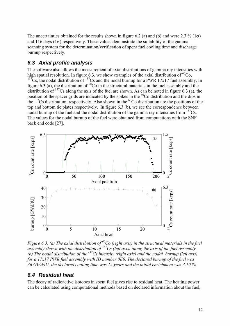
The uncertainties obtained for the results shown in figure 6.2 (a) and (b) and were 2.3 % (1σ) and 116 days (1σ) respectively. These values demonstrate the suitability of the gamma scanning system for the determination/verification of spent fuel cooling time and discharge burnup respectively.

6.3 Axial profile analysis The software also allows the measurement of axial distributions of gamma ray intensities with high spatial resolution. In figure 6.3, we show examples of the axial distribution of 60Co, 137Cs, the nodal distribution of 137Cs and the nodal burnup for a PWR 17x17 fuel assembly. In figure 6.3 (a), the distribution of 60Co in the structural materials in the fuel assembly and the distribution of 137Cs along the axis of the fuel are shown. As can be noted in figure 6.3 (a), the position of the spacer grids are indicated by the spikes in the 60Co distribution and the dips in the 137Cs distribution, respectively. Also shown in the 60Co distribution are the positions of the top and bottom tie plates respectively. In figure 6.3 (b), we see the correspondence between nodal burnup of the fuel and the nodal distribution of the gamma ray intensities from 137Cs. The values for the nodal burnup of the fuel were obtained from computations with the SNF back end code [27].

0 50 100 150 2000

6.5

137 Cs

cou

nt ra

te [k

cps]

Axial position0 50 100 150 200

0

1.5

60Cs

cou

nt ra

te [k

cps]

0 5 10 15 200

10

20

30

40

burn

up [G

Wd/

tU]

Axial level0 5 10 15 20

0

6.3

137 Cs

cou

nt ra

te [k

cps]

(a)

(b)

Figure 6.3. (a) The axial distribution of 60Co (right axis) in the structural materials in the fuel assembly shown with the distribution of 137Cs (left axis) along the axis of the fuel assembly. (b) The nodal distribution of the 137Cs intensity (right axis) and the nodal burnup (left axis) for a 17x17 PWR fuel assembly with ID number 0E6. The declared burnup of the fuel was 36 GWd/tU, the declared cooling time was 15 years and the initial enrichment was 3.10 %.

6.4 Residual heat The decay of radioactive isotopes in spent fuel gives rise to residual heat. The heating power can be calculated using computational methods based on declared information about the fuel,

12

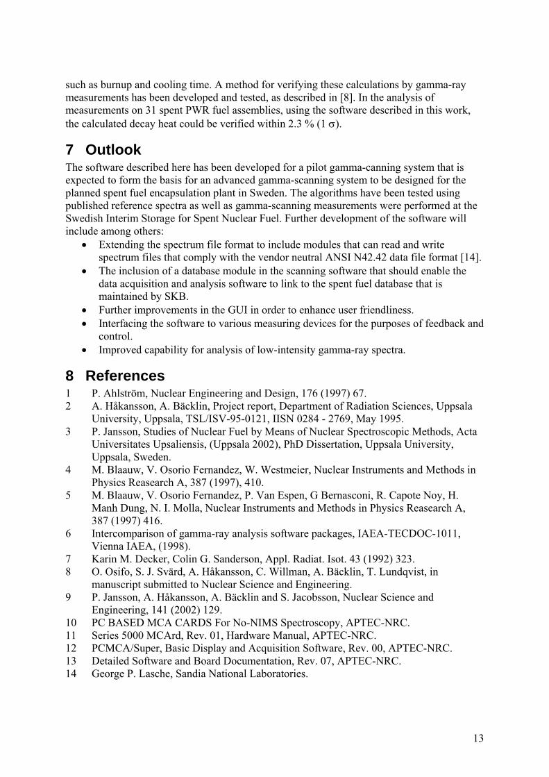
such as burnup and cooling time. A method for verifying these calculations by gamma-ray measurements has been developed and tested, as described in [8]. In the analysis of measurements on 31 spent PWR fuel assemblies, using the software described in this work, the calculated decay heat could be verified within 2.3 % (1 σ).

7 Outlook The software described here has been developed for a pilot gamma-canning system that is expected to form the basis for an advanced gamma-scanning system to be designed for the planned spent fuel encapsulation plant in Sweden. The algorithms have been tested using published reference spectra as well as gamma-scanning measurements were performed at the Swedish Interim Storage for Spent Nuclear Fuel. Further development of the software will include among others:

• Extending the spectrum file format to include modules that can read and write spectrum files that comply with the vendor neutral ANSI N42.42 data file format [14].

• The inclusion of a database module in the scanning software that should enable the data acquisition and analysis software to link to the spent fuel database that is maintained by SKB.

• Further improvements in the GUI in order to enhance user friendliness. • Interfacing the software to various measuring devices for the purposes of feedback and

control. • Improved capability for analysis of low-intensity gamma-ray spectra.

8 References 1 P. Ahlström, Nuclear Engineering and Design, 176 (1997) 67. 2 A. Håkansson, A. Bäcklin, Project report, Department of Radiation Sciences, Uppsala

University, Uppsala, TSL/ISV-95-0121, IISN 0284 - 2769, May 1995. 3 P. Jansson, Studies of Nuclear Fuel by Means of Nuclear Spectroscopic Methods, Acta

Universitates Upsaliensis, (Uppsala 2002), PhD Dissertation, Uppsala University, Uppsala, Sweden.

4 M. Blaauw, V. Osorio Fernandez, W. Westmeier, Nuclear Instruments and Methods in Physics Reasearch A, 387 (1997), 410.

5 M. Blaauw, V. Osorio Fernandez, P. Van Espen, G Bernasconi, R. Capote Noy, H. Manh Dung, N. I. Molla, Nuclear Instruments and Methods in Physics Reasearch A, 387 (1997) 416.

6 Intercomparison of gamma-ray analysis software packages, IAEA-TECDOC-1011, Vienna IAEA, (1998).

7 Karin M. Decker, Colin G. Sanderson, Appl. Radiat. Isot. 43 (1992) 323. 8 O. Osifo, S. J. Svärd, A. Håkansson, C. Willman, A. Bäcklin, T. Lundqvist, in

manuscript submitted to Nuclear Science and Engineering. 9 P. Jansson, A. Håkansson, A. Bäcklin and S. Jacobsson, Nuclear Science and

Engineering, 141 (2002) 129. 10 PC BASED MCA CARDS For No-NIMS Spectroscopy, APTEC-NRC. 11 Series 5000 MCArd, Rev. 01, Hardware Manual, APTEC-NRC. 12 PCMCA/Super, Basic Display and Acquisition Software, Rev. 00, APTEC-NRC. 13 Detailed Software and Board Documentation, Rev. 07, APTEC-NRC. 14 George P. Lasche, Sandia National Laboratories.

13

15 G. Gilmore, J. Hemingway,Practical Gamma-Ray Spectroscopy, John Wiley & Sons 2003.

16 International safety research (ISR), Technical note ISR TN-1030-3, version 1.5, 1 May 2000.

17 V. Hnatowicz, Nuclear Instruments and methods 133 (1976) 137. 18 J. D. Valentine, IEEE Transaction on Nuclear Science, 43, (1996) 2501. 19 P. B. R. Björkholm and A. T. Dyring, A Study of a High Rate Gamma-Spectrometer

System for Burnup Measurements, M.Sc Thesis, School of Engineering, Uppsala University, UPTEC 90 015E.

20 T. D Reilly, J. L. Parker, A Guide to Gamma-Ray Assay for Nuclear Material Accountability, LA-5794-M, 1975, report, Los Alamos Scientific Laboratory.

21 J. L. Parker, General Topics in Passive Gamma-Ray Assay (Chapter 5 in NUREG 550-1990, Passive Nondestructive Assay of Nuclear Materials, Edited by T. D. Reilly, N. Esslin and H. Smith Jr).

22 P. C. L. da Costa, C. C. Dantas, C.A.B.O. Lira, V.A. dos Santos, Nuclear Instruments and Methods in Physics Reasearch B 226 (2004), 419.

23 Gamma-Ray Spectrum Catalogue, Ge and Si Detector Spectra, Fourth Edition, Idaho National Engineering and Environmental Laboratory, Gamma-ray spectrometry center. Web page: http://www.inl.gov/gammaray/catalogs/pdf/. Last accessed: December, 14, 2006.

24 U. Reus, W. Westmeier, Atomic Data and Nuclear Data Tables 29, (1983) 193-406. 25 P. JANSSON, “Studies of Nuclear Fuel by Means of Nuclear Spectroscopic Methods,”

PhD Thesis, Uppsala University (2002). 26 C. Willman, A. Håkansson, O. Osifo, A. Bäcklin and S. Jacobsson Svärd, “Non-

destructive assay of Spent Nuclear Fuel with Gamma-Ray Spectroscopy,” Annals of Nuclear Energy, 33, 427 (2006).

27 S. Børresen and M. Kruners “Validation of SNF Against CLAB Decay Heat Measurements,” SSP-04/216, report, Studsvik Scandpower (2005).

14

Verification and determination of the decay heat in spent PWR fuel by means of gamma scanning

Otasowie Osifo, Staffan Jacobsson Svärd, Ane Håkansson, Christofer Willman,

Anders Bäcklin, Tobias Lundqvist

Uppsala University, Department of Neutron Research, Box 525, SE-751 20, Uppsala, Sweden

Abstract Decay heat is an important design parameter at the future Swedish spent nuclear fuel repository. It will be calculated for each fuel assembly using dedicated depletion codes, based on the operator-declared irradiation history. However, experimental verification of the calculated decay heat is also anticipated. Such verification may be obtained by gamma scanning, using the established correlation between the decay heat and the emitted gamma-ray intensity from 137Cs. In this procedure, also the correctness of the operator-declared fuel parameters may be verified.

Recent achievements of the gamma scanning technique include the development of a dedicated spectroscopic data-acquisition system and the use of an advanced calorimeter for calibration. Using this system, the operator-declared burnup and cooling time of 31 PWR fuel assemblies was verified experimentally to within 2.2% (1 σ) and 1.9 % (1 σ), respectively. The measured decay heat agreed with calorimetric data within 2.3% (1 σ), whereby the calculated decay heat was verified within 2.3 % (1 σ). The measuring time per fuel assembly was about 15 minutes.

In case reliable operator-declared data is not available, the gamma-scanning technique also provides a means to independently measure the decay heat. The results obtained in this procedure agreed with calorimetric data within 2.7 % (1 σ).

I INTRODUCTION The problem of disposing of spent nuclear fuel generated from the operation of nuclear reactors is being addressed by the world community and is regarded as a high priority issue that must be solved in a safe and secure manner.

The Swedish concept for dealing with the problem is based on the encapsulation of the fuel assemblies in copper canisters. The canisters will in turn be embedded in bentonite clay that serves as a buffer in a deep geological storage.1 To maintain the buffer properties of the bentonite clay, an upper limit of 100°C for the temperature on the surface of the copper canisters has been defined.2, ,3 4

Initially, the discharged fuel assemblies from the reactors will be stored in an interim

storage site for a time period of between 15 and 50 years, with a typical value of 30 years. After this cooling time, it is still important to achieve a firm knowledge of the decay heat generated by each fuel assembly in the canisters to ensure that the temperature limit is not exceeded.

One of the methods available for the determination of the decay heat of a spent nuclear fuel assembly is the use of depletion codes5 such as ORIGEN-ARP. These codes generally calculate decay heat with typical accuracies ranging between 2% and 5%.6 Obviously, the accuracy of any depletion calculation is dependent on the authenticity and accuracy of the input data. From an operational point of view as well as from a safeguards point of view, the effect of such dependence must be relaxed. This may be achieved either by using an

1

independent experimental technique to determine the decay heat or by using a measuring technique that enables verification of the calculations. An independent experimental technique for the measurement of decay heat that has been proven to be highly accurate is calorimetry7,8. However, this technique implies measuring times of the order of days per assembly. These long measurement times are not considered practical for industrial applications, therefore the gamma-scanning technique has been proposed as an alternative method9,10. It should be noted that the gamma scanning system must be calibrated for application in the measurement of decay heat. The calibration of the gamma scanning system against calorimetry is one of the focal points in this report.

As a complement to pure theoretical approaches, the gamma-scanning technique provides

the following two advantages: i. First, in normal cases where operator-declared data are available, the technique provides

a means for verifying the calculated decay heat by using experimentally measured gamma-ray intensities.

ii. Secondly, as is shown in this work, if declared information is questionable or unavailable, a determination of the decay heat may still be performed.

The current paper accounts for an extension of the work on gamma scanning presented in references 9 and 10. Here the efforts have been focused on the following items:

i. New data-acquisition and analysis software has been developed and used in the experimental part of this work.

ii. A new calorimeter has been designed and constructed in order to improve the accuracy in the calibration. More detailed information on this device can be found in ref. 11.

iii. The applicability of the method for verification of calculated decay heat has been demonstrated in comparisons with data obtained from the Spent Nuclear Fuel depletion code (SNF)12.

iv. The feature of the method to yield decay-heat information independently of operator-declared information has been emphasized. It has been explicitly shown how experimentally obtained values of burnup and cooling time are used to determine the decay heat.

II METHOD

II.A Overview The method of determining the decay heat by measuring the gamma-ray intensity

associated with the beta decay of 137Cs has been described in refs. 9 and 10. It was shown that the gamma-ray intensity of the 137Cs decay could be used to verify the decay heat of spent nuclear fuel assemblies with a relative accuracy of about 3%.

The linear relationship established between the decay heat P of a fuel assembly and the

measured intensity I137 (due to the decay of 137Cs) is defined by: 137 IP Cf

= ⋅ (2.1)

In eq. (2.1), C is a proportionality constant, determined through a calibration procedure as described in section II.D, f is the fractional decay heat from the decay of 137Cs, defined by:

PP

f 137= (2.2)

2

Where P137 is the power developed in the fuel due to the decay of 137Cs. The fractional decay heat (f) is more elaborately described in section II.B. The methodology thus consists of the following steps:

i. Calculation of f for each fuel geometry of interest as a function of burnup and cooling time using a properly validated code e.g. ORIGEN-ARP.

ii. From these calculations, determine simple expressions of f as a function of burnup and cooling time.

iii. Determine calibrations constants C for each fuel geometry of interest by correlating calorimetrically determined decay heat with measured 137Cs intensities.

iv. For a specific fuel assembly, its operator declared burnup and cooling time are verified using the method suggested in ref. 13. In a case where no operator data is available the method of ref. 13 provides the adequate values on burnup and cooling time.

v. Inserting these values on burnup and cooling time into the expression for f yields, together with C and the measured 137Cs intensity, the decay heat of the fuel assembly.

Although not directly measured, the decay heat of a specific fuel assembly is determined by using measured quantities for determining the calibration constants C. Also the corresponding gamma-ray intensity, 137Cs, in eq. (2.1), stems from measurements. Although f is based on calculations, only its generic dependency on burnup and cooling time is used. This means that whenever the burnup and cooling time of a fuel assembly is known, either by using measurements13 or by using verified operator declared values, f can be easily estimated. In this paper the decay heat determined in accordance with the steps above will therefore be denoted as “measured” decay heat.

II.B The fractional decay heat, f, from 137Cs The fractional contribution from 137Cs to the total decay heat, f, was defined in eq. (2.2). To

illustrate the dependence of f on some fuel parameters, we show in figures 2.1, 2.2 and 2.3 f as a function of the cooling time, burnup and enrichment, respectively. The data presented here was calculated for PWR 17x17 fuel assemblies using ORIGEN-ARP.

0 10 20 30 40 50 600

0.1

0.2

0.3

0.4

Cooling time [years]

Frac

tiona

l con

tribu

tion

(f)

Figure 2.1. The fractional power f as a function of the cooling time for PWR 17x17 fuel irradiated for five power cycles. The discharge burnup was 36 GWd/tU and the initial enrichment was 3.1 %. The figure shows that for cooling time in the range of 15 to 50 years, the relative variation of f is about –0.6 % per year.

3

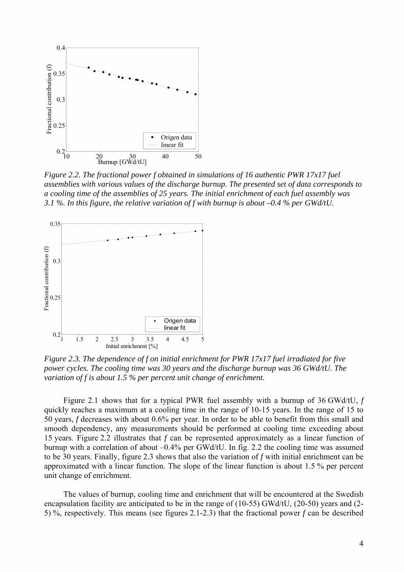
10 20 30 40 500.2

0.25

0.3

0.35

0.4

Burnup [GWd/tU]

Frac

tiona

l con

tribu

tion

(f)

Origen datalinear fit

Figure 2.2. The fractional power f obtained in simulations of 16 authentic PWR 17x17 fuel assemblies with various values of the discharge burnup. The presented set of data corresponds to a cooling time of the assemblies of 25 years. The initial enrichment of each fuel assembly was 3.1 %. In this figure, the relative variation of f with burnup is about –0.4 % per GWd/tU.

1 1.5 2 2.5 3 3.5 4 4.5 50.2

0.25

0.3

0.35

Initial enrichment [%]

Frac

tiona

l con

tribu

tion

(f)

Origen datalinear fit

Figure 2.3. The dependence of f on initial enrichment for PWR 17x17 fuel irradiated for five power cycles. The cooling time was 30 years and the discharge burnup was 36 GWd/tU. The variation of f is about 1.5 % per percent unit change of enrichment.

Figure 2.1 shows that for a typical PWR fuel assembly with a burnup of 36 GWd/tU, f

quickly reaches a maximum at a cooling time in the range of 10-15 years. In the range of 15 to 50 years, f decreases with about 0.6% per year. In order to be able to benefit from this small and smooth dependency, any measurements should be performed at cooling time exceeding about 15 years. Figure 2.2 illustrates that f can be represented approximately as a linear function of burnup with a correlation of about –0.4% per GWd/tU. In fig. 2.2 the cooling time was assumed to be 30 years. Finally, figure 2.3 shows that also the variation of f with initial enrichment can be approximated with a linear function. The slope of the linear function is about 1.5 % per percent unit change of enrichment.

The values of burnup, cooling time and enrichment that will be encountered at the Swedish encapsulation facility are anticipated to be in the range of (10-55) GWd/tU, (20-50) years and (2-5) %, respectively. This means (see figures 2.1-2.3) that the fractional power f can be described

4

by simple functions, which, in turn, implies that the method described in this paper, in principle, is expected to fulfil reasonable demands on robustness and accuracy.

In this work, a parameterization in terms of burnup and cooling time has been applied for obtaining f. As stated above, there is a linear dependence in burnup. In addition, the exponential decay of the radioactive isotopes motivate, after expansion to the second order in time, a quadratic dependency on cooling time T, once passing a time T0 when the f factor has peaked (see figure 2.1). Accordingly, the following parameterization is obtained:

f (Bu,T) = A0 + A1Bu + A2(T – T0) + A3(T – T0)2 (2.3)

Here, the value of T0 was set to 14 years, thus allowing only cooling times longer than 14 years to be analyzed. As is evident from eq. (2.3), the dependency on initial enrichment has been omitted in the present analysis. This is motivated by the mild dependency of f on initial enrichment noted above, affecting the determined decay heat with an amount within the experimental uncertainty.

In this work, the values of the coefficients A0, A1, A2 and A3 were determined for each of the investigated fuel geometries by fitting f, obtained from ORIGEN-ARP calculations to burnup and cooling time. For the calculations of f, the burnup was varied in the interval: Bu = (15-50) GWd/tU in steps of 3.0 GWd/tU while the cooling time was varied in the interval: T = (15-50) years in steps of 600 days. The enrichment was kept at a constant value of 3 % for the fuel assemblies studied here.

In this study, two fuel geometries were included, namely PWR 15x15 and PWR 17x17. The values of the fitting coefficients for these two fuel geometries are presented in table I.

Table I. Numerical values of the fitting coefficients An of eq. (2.3). The uncertainty for each coefficient is given (1 σ).

Fuel geometry A0A1

[10-3tU/GWd] A2

[10-3 yrs-1] A3

[10-5yrs-2] 15x15 17x17

0.415 ± 0.003 0.415 ± 0.003

-1.47 ± 0.06 -1.51 ± 0.06

-1.46± 0.28 -1.47 ± 0.28

-2.07 ± 1.05 -2.12 ± 1.04

II.C Application of the method As indicated in section I, depending on the availability of reliable operator-declared data

for a fuel assembly, two possible scenarios can be envisaged in the application of the gamma-scanning method:

Case (i): Verification of decay-heat calculations. Here the declared burnup and cooling time are used in order to obtain f. To verify the correctness of the declared burnup and cooling time, these parameters are determined by using the method of reference 13. Case (ii): Determination of decay heat in cases where operator-declared information could not be satisfactorily verified or the computation of the decay heat could not be performed. Here the burnup and cooling time, as determined by using the method of reference 13, is used for obtaining f.

To apply the gamma scanning system in either of these two cases, it is necessary to

determine the discharge burnup and the cooling time for the fuel assembly under investigation.

5

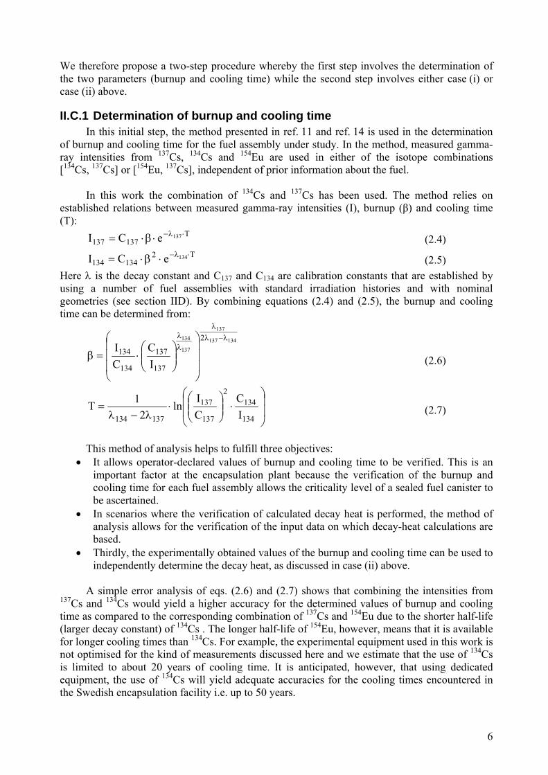
We therefore propose a two-step procedure whereby the first step involves the determination of the two parameters (burnup and cooling time) while the second step involves either case (i) or case (ii) above.

II.C.1 Determination of burnup and cooling time In this initial step, the method presented in ref. 11 and ref. 14 is used in the determination

of burnup and cooling time for the fuel assembly under study. In the method, measured gamma-ray intensities from 137Cs, 134Cs and 154Eu are used in either of the isotope combinations [134Cs, 137Cs] or [154Eu, 137Cs], independent of prior information about the fuel.

In this work the combination of 134Cs and 137Cs has been used. The method relies on

established relations between measured gamma-ray intensities (I), burnup (β) and cooling time (T):

T137137

137eCI ⋅λ−⋅β⋅= (2.4) T2

134134134eCI ⋅λ−⋅β⋅= (2.5)

Here λ is the decay constant and C137 and C134 are calibration constants that are established by using a number of fuel assemblies with standard irradiation histories and with nominal geometries (see section IID). By combining equations (2.4) and (2.5), the burnup and cooling time can be determined from:

134137

137

137

134 2

137

137

134

134

IC

CI

λ−λλ

λλ

⎟⎟⎟

⎠

⎞

⎜⎜⎜

⎝

⎛

⎟⎟⎠

⎞⎜⎜⎝

⎛⋅=β (2.6)

⎟⎟

⎠

⎞

⎜⎜

⎝

⎛⋅⎟⎟

⎠

⎞⎜⎜⎝

⎛⋅

λ−λ=

134

1342

137

137

137134 IC

CI

ln2

1T (2.7)

This method of analysis helps to fulfill three objectives:

• It allows operator-declared values of burnup and cooling time to be verified. This is an important factor at the encapsulation plant because the verification of the burnup and cooling time for each fuel assembly allows the criticality level of a sealed fuel canister to be ascertained.

• In scenarios where the verification of calculated decay heat is performed, the method of analysis allows for the verification of the input data on which decay-heat calculations are based.

• Thirdly, the experimentally obtained values of the burnup and cooling time can be used to independently determine the decay heat, as discussed in case (ii) above.

A simple error analysis of eqs. (2.6) and (2.7) shows that combining the intensities from 137Cs and 134Cs would yield a higher accuracy for the determined values of burnup and cooling time as compared to the corresponding combination of 137Cs and 154Eu due to the shorter half-life (larger decay constant) of 134Cs . The longer half-life of 154Eu, however, means that it is available for longer cooling times than 134Cs. For example, the experimental equipment used in this work is not optimised for the kind of measurements discussed here and we estimate that the use of 134Cs is limited to about 20 years of cooling time. It is anticipated, however, that using dedicated equipment, the use of 134Cs will yield adequate accuracies for the cooling times encountered in the Swedish encapsulation facility i.e. up to 50 years.

6

II.C.2 Case (i): verification of the calculated decay heat In this case, operator declared information is assumed to be available and this information

is subject to verification. For a fuel assembly of interest, the operator-declared burnup and cooling time are thus experimentally determined by using eqs. (2.6) and (2.7). If the differences between these values and the corresponding operator declared values are less than a suitably defined amount, either the declared values or the measured values can be used in eq. (2.3) in order to obtain the decay heat. If correct, the declared decay heat value should equal the measured value within the limits of experimental and computational uncertainties.

II.C.3 Case (ii): independent determination of the decay heat In scenarios where part of the declared information is lacking, questionable or otherwise

not feasible to use for calculations, the gamma-scanning method still offers the possibility to determine decay heat within a few percent. This is accomplished by using the method described by eq. (2.6) and eq. (2.7) to determine the burnup and cooling time. From this information, the value f is estimated using eq. (2.3) whereby the decay heat follows from eq. (2.1).

II.D Calibration and normalization procedure To obtain the proportionality constant C in eq. (2.1), a calibration is performed. The first

step of such a calibration is to identify a number of fuel assemblies that can be considered as “normal” in every aspect (here called reference assemblies). In this context, normal means that no reconstruction of the assemblies has taken place and that the irradiation histories are consistent with regular reactor operation. The reference assemblies are further divided into two main groups: a group of BWR reference assemblies and a group of PWR reference assemblies.

The number of reference assemblies is a matter of statistical considerations. Clearly, the

more reference assemblies included in the calibration procedure, the higher will the accuracy be. Therefore we have adopted an iterative strategy implying that every fuel assembly that is measured and where its burnup, cooling time and decay heat is successfully verified, will be included into the list of reference assemblies. Presently, there are eleven 15x15 PWR and thirteen 17x17 PWR in the list of reference assemblies.

As the constant C is strongly dependent on the measuring geometry as well as the fuel

geometry9, ,10 14, C must be established for each fuel geometry of interest within each main group. This requirement is relaxed if one considers renormalization of the data with the aid of calculated gamma transport coefficients using a suitable computer code such as the one presented in reference 20 and briefly discussed in section VIII.

In a second step of the calibration procedure, the measured gamma-ray intensities of the

reference assemblies, properly corrected for f, are correlated to their corresponding decay heat obtained from the calorimetric measurements (briefly described in section IV.B.1).

The geometry dependence of C also implies that even small changes on measuring

geometry will cause large effects on the results. Specifically it can be concluded that a new measuring campaign must be normalized to the existing calibration. In references 9,10 it is described how to use the reference assemblies in the normalization procedure.

In this work, only one measurement campaign was performed, where the calibration was

established and therefore no normalization was required.

7

III GAMMA SCANNING EQUIPMENT Below is a brief presentation of the equipment used in the gamma scanning measurements

described in this paper. More elaborate descriptions can be found in refs. 10, 11 and 16.

III.A Mechanical equipment Referring to fig. 3.1, a mechanical fixture mounted in a fuel handling pool is used to hold

the fuel assembly in front of a collimator mounted in the pool wall. The fuel assembly is moved vertically across the collimator by an elevator system. The fixture also makes it possible to rotate the assembly so that a corner is facing the collimator, which makes the measured gamma-ray intensities relatively insensitive to positioning uncertainties14.

Figure 3.1. Schematic view over the mechanical equipment used for the measurements. To the left is a top view of the collimator-detector arrangement and to the right is a side view of the system. The equipment shown is originally designed for other purposes and is not optimized for the type of measurements reported here.

The collimator is made of iron with a length of 1.2 m. The slit is horizontal and its height can be varied between 1 mm and 3 mm. The width varies from 243 mm at the end facing the fuel assembly to 82 mm at the end facing the detector. This arrangement allows for a solid angle covering the diagonal of all fuel types of interest. The gamma-ray detector and the data-acquisition system are located behind the collimator in a separate room, on the dry side of the pool wall.

8

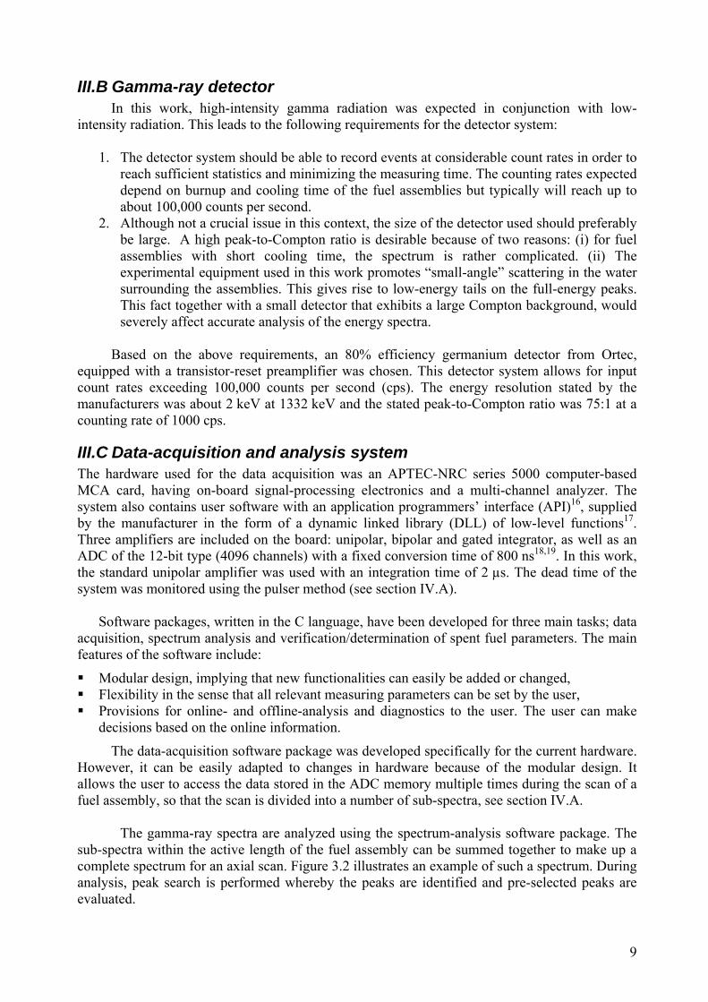
III.B Gamma-ray detector In this work, high-intensity gamma radiation was expected in conjunction with low-

intensity radiation. This leads to the following requirements for the detector system:

1. The detector system should be able to record events at considerable count rates in order to reach sufficient statistics and minimizing the measuring time. The counting rates expected depend on burnup and cooling time of the fuel assemblies but typically will reach up to about 100,000 counts per second.

2. Although not a crucial issue in this context, the size of the detector used should preferably be large. A high peak-to-Compton ratio is desirable because of two reasons: (i) for fuel assemblies with short cooling time, the spectrum is rather complicated. (ii) The experimental equipment used in this work promotes “small-angle” scattering in the water surrounding the assemblies. This gives rise to low-energy tails on the full-energy peaks. This fact together with a small detector that exhibits a large Compton background, would severely affect accurate analysis of the energy spectra.

Based on the above requirements, an 80% efficiency germanium detector from Ortec,

equipped with a transistor-reset preamplifier was chosen. This detector system allows for input count rates exceeding 100,000 counts per second (cps). The energy resolution stated by the manufacturers was about 2 keV at 1332 keV and the stated peak-to-Compton ratio was 75:1 at a counting rate of 1000 cps.

III.C Data-acquisition and analysis system The hardware used for the data acquisition was an APTEC-NRC series 5000 computer-based MCA card, having on-board signal-processing electronics and a multi-channel analyzer. The system also contains user software with an application programmers’ interface (API)16, supplied by the manufacturer in the form of a dynamic linked library (DLL) of low-level functions17. Three amplifiers are included on the board: unipolar, bipolar and gated integrator, as well as an ADC of the 12-bit type (4096 channels) with a fixed conversion time of 800 ns18,19. In this work, the standard unipolar amplifier was used with an integration time of 2 µs. The dead time of the system was monitored using the pulser method (see section IV.A).

Software packages, written in the C language, have been developed for three main tasks; data acquisition, spectrum analysis and verification/determination of spent fuel parameters. The main features of the software include:

Modular design, implying that new functionalities can easily be added or changed, Flexibility in the sense that all relevant measuring parameters can be set by the user, Provisions for online- and offline-analysis and diagnostics to the user. The user can make

decisions based on the online information.

The data-acquisition software package was developed specifically for the current hardware. However, it can be easily adapted to changes in hardware because of the modular design. It allows the user to access the data stored in the ADC memory multiple times during the scan of a fuel assembly, so that the scan is divided into a number of sub-spectra, see section IV.A.

The gamma-ray spectra are analyzed using the spectrum-analysis software package. The

sub-spectra within the active length of the fuel assembly can be summed together to make up a complete spectrum for an axial scan. Figure 3.2 illustrates an example of such a spectrum. During analysis, peak search is performed whereby the peaks are identified and pre-selected peaks are evaluated.

9

0 0.5 1 1.5 2 2.5 3

102

104

106

photon energy [MeV]

coun

ts p

er c

hann

el

Figure 3.2. Example of a spectrum obtained in a scan. The collection time for this spectrum was 167 s. The data was collected for a PWR 17x17 fuel assembly with ID number 3C1, having a declared burnup of 36.6 GWd/tU and a declared cooling time of about 16.6 years. The prominent peak on the left-hand side of the spectrum corresponds to the decay of 137Cs while the peak on the right-hand side of the spectrum is the peak from a pulse generator (see section IV.A).

In particular, the spectrum-analysis software calculates and presents the axial distributions

of the relative isotopic intensities of the radionuclides 154Eu, 137Cs and 134Cs. However, it is possible for the user to select more isotopes or a different set of isotopes for the analysis.

Figure 3.3 shows an example of the axial distribution of the relative intensity of 137Cs for a PWR 17x17 fuel assembly. Also presented is the nodal burnup of the fuel along the fuel axis, as obtained from computations using the SNF code12. The figure demonstrates the usefulness of 137Cs for deducing the burnup profile of a fuel assembly.

0 5 10 15 20 250

10

20

burn

up [G

Wd/

tU]

Axial level

Axial burnup distribution Axial distribution of Cs-137

0 5 10 15 20 25

1

2

3

Cs-

137

coun

t rat

e [k

cps]

Figure 3.3. The axial distribution of the 137Cs intensity (right axis) and the burnup (left axis) for a 17X17 PWR fuel assembly with ID number 5A3. The declared burnup of the fuel was 20 GWd/tU, the declared cooling time was 18.7 years and the initial enrichment was 2.1%.

Finally, a software package has been developed that accounts for the

verification/determination of spent fuel parameters, in particular the decay thermal power. It includes abilities such as calculating burnup and cooling time for a specific fuel assembly, according to the techniques discussed in section II.C.1. It interacts with a database including operator-declared parameters and the results from computational codes and calorimetric

10

measurements when available. In the current development stage, it also includes the determination of the calibration constant C.

It can be noted that the software directly can present information of the decay heat to the user. Presently, the output from the analysis package is also written to comma-separated-value files that may be opened in utility software such as Microsoft Excel© for further computations and analysis.

IV EXPERIMENTAL STUDY The scope of this study was to perform a calibration of a pilot gamma-scanning system for

application in decay heat measurements, using a new calorimeter 11 and to demonstrate the attainable accuracy of the gamma-scanning technique. As discussed in section II.C, the study has been divided into two parts, depending on which information that is considered to be available: (i) operator-declared data is considered to be available, making the gamma-scanning measurements a verification of the calculated decay heat, and (ii) cases where no prior information about the fuel assemblies is used, except for knowledge of the assembly type, making the gamma-scanning measurements a stand-alone determination of the decay heat. The results from the first case are presented in section V.C while the results from the second case are presented in section V.D

IV.A Gamma scanning procedure The gamma scanning of a fuel assembly was performed with the fuel assembly placed in

the mechanical fixture briefly described in section III.A. The fixture was rotated so that a corner of the fuel assembly faced the detector (see fig. 3.1). When data taking was started, the fuel assembly was moved vertically across the collimator and the data acquisition system recorded 210 sub-spectra along the assembly. When the scan was finished, the assembly was rotated so that the next corner faced the collimator and the scanning procedure was repeated until all four corners were scanned.

In this work, the speed of the elevator carrying the fuel assembly (scanning speed) was set to about 120 cm per minute in the upward direction and about 150 cm per minute in the downward direction implying a mean scanning time of about 3.5 minutes per corner. These speeds were considered a feasible compromise between measuring times and uncertainties due to counting statistics.

The different scanning speeds implied that when an assembly was moving in the upward direction, the data collecting time for each sub-spectrum was set to 1.26 seconds and in the downward direction to 1.01 seconds. A total of 210 sub-spectra per corner were collected, covering somewhat more than the active length of the fuel assembly.

In total, the measuring time per assembly was about 15 minutes. Including fuel handling,

the measurements were performed at a typical rate of one fuel assembly every 30 minutes. In the measurements performed here, gross input count rates reaching about 80,000 cps

were encountered. This together with the performance of the detector system implied dead-time losses that varied from a few percent up to about 50 % (assembly F32). Corrections for count rate losses (dead time and pileup) were performed using the pulser method9,10 where tail pulses from a pulse generator were introduced into the detection system. The frequency of the input was set to (2000 ± 1) Hz. By forming the ratio between the input and the output count rates of the injected

11

signal, dead-time correction factors for each subspectrum were obtained. Assuming a paralyzable model for the dead time, the relative uncertainty of the correction factors were found to be, in general, of the order of 10-2, which was considered to be sufficiently small to be neglected in this context.

IV.B Data used for calibration and evaluation

IV.B.1 Calorimetrically measured decay heat Calorimetric measurements were performed by SKB (The Swedish Nuclear Fuel and Waste

Management Co.) using the new calorimeter, as described in reference 11. In that report, a detailed account of the measuring principle, calibration procedure (for the calorimeter) and resulting measuring data was made and thus only a brief description will be given here.

The calorimeter is designed to perform decay-heat measurements in the range of (50 -

1000) W and it is operational for both PWR and BWR fuel assemblies. The design goal was to determine the decay heat within 2% (2 σ)11.

The calorimeter is constructed for submergence into one of the fuel handling ponds at the CLAB facility. The principle is to monitor the temperature increase, due to the decay heat, within a water-filled, thermally isolated and closed vessel until a steady-state temperature has been reached. A calorimetric measurement takes typically about 24 hours.

During calorimetric measurements, some part of the gamma radiation emitted by a fuel

assembly escapes the calorimeter vessel. Corrections to the measured decay heat must be made to account for these losses. A notable feature of the new calorimeter is the possibility to map the gamma-radiation field in the surrounding water, by using gamma-ray dosimeters mounted outside the calorimeter, and including that contribution in the measured total decay heat. The contribution to the decay heat from this gamma radiation was estimated in this work to be in the range of 2 - 3% for the cooling times encountered here, i.e. (15-22) years11.

IV.B.2 Calculated decay heat In a separate project,12 Studsvik Scandpower has calculated the decay heat using the SNF

code for a large number of fuel assemblies, including the assemblies in this study. The spent nuclear fuel program (SNF) is a coupled code that can be used to calculate the isotopic inventories and the decay heat of spent nuclear fuel. The input to SNF is constituted by the output from the lattice and nodal analysis codes: CASMO and SIMULATE. The details of the method used in the calculations and the results are presented in ref. 12

At the Swedish encapsulation plant, calculations using available operator-declared data will

constitute one of the strategies for the determination of decay heat. However, it is considered desirable to verify the correctness of these calculations experimentally. Accordingly, the data from ref. 12 has in this study been used to demonstrate the capability of the gamma-scanning technique for such verification.

IV.C Fuel assemblies included in this work The measurements using the gamma scanning technique were performed during three

campaigns. A total number of 92 assemblies from 10 reactors were scanned. The decay heat of each assembly was also measured using the calorimetric method. To ascertain the repeatability of the measurements, the decay heat of a given set of fuel assemblies was measured in each of the three measuring campaigns, calorimetric as well as by gamma scanning.

12

From the total of 92 assemblies scanned, 24 PWR assemblies were chosen for the

calibration procedure, based on the following criteria: • The assemblies had to be measured calorimetrically, • Calculations of the decay heat had to be made with the SNF code, • The assemblies had to be part of a larger set (>10) of the same fuel type, • The assemblies should not have been rebuilt or reconstructed, • The irradiation history should not include irregularities such as outages of one irradiation

cycle or more.

The main data of the fuel assemblies are displayed in table II. In the table, we show the values of operator-declared fuel parameters as well as the decay heat for each fuel assembly as obtained from the calorimetric measurements. We also show the calculated decay heat obtained from the SNF code. It can be noted that the agreement between the calorimetrically measured and the calculated decay heat in table II is 1.0% (1 σ), giving an estimate of the accuracy of the calculated data.

To get an impression of the impact of irregular fuel parameters on the results, assemblies 2A5, 5A3, C01, C12, D27, I20 and F32 were also included in the further analysis. For C01, C12 and D27, the irradiation history included an outage of one year while F32 had experienced an outage of two years. The irradiation histories of 2A5 and 5A3 exhibit an extended first power cycle lasting for three years. I20, on the other hand was reconstructed in such a way that two fuel rods were removed after discharge. In table III other relevant information of these assemblies are shown.

13

Table II. The fuel assemblies used in the calibration procedure. The table shows values of the operator-declared initial enrichment (ε), discharge burnup (BU) and cooling time (CT). Also shown are the values of the decay heat obtained from the calorimetric measurements for each fuel assembly. Finally, the calculated values of the decay heat are given. Note that assembly E38 was measured twice.

Fuel ID

Fuel geometry

ε

[%]

Decl. BU

[GWd/tU]

Decl. CT

[y]

Decay heat(calorimetry)

[W]

Decay heat(SNF) [W]

0E6 3C5 0C9 1C2 1C5 2C2 3C1 3C4 3C9 4C4 4C7 0E2 1E5 I24 I09 F25 D38 E38 E38 E40 F14 F21 G11 G23 I25

17x17 " " " " " " " " " " " "

15x15 " " " " " " " " " " "

3.10 3.10 3.10 3.10 3.10 3.10 3.10 3.10 3.10 3.10 3.10 3.10 3.10 3.20 3.20 3.20 3.25 3.20 3.20 3.20 3.20 3.20 3.19 3.21 3.20

35.99 38.37 38.44 33.32 38.48 36.58 36.57 38.45 36.56 33.33 38.37 41.63 34.64 34.34 40.19 35.35 39.40 33.97 33.97 34.34 34.01 36.27 35.46 35.63 36.86

14.53 16.63 16.63 16.63 16.63 16.63 16.63 16.63 16.63 16.64 16.63 14.52 14.52 16.73 14.68 19.72 20.69 20.69 20.71 20.70 19.72 18.76 17.79 17.79 15.72

487.7 ± 5.5 501.4 ± 5.6 491.2 ± 5.5417.7 ± 5.2499.2 ± 5.6466.5 ± 5.4 470.2 ± 5.4497.3 ± 5.6 468.4 ± 5.4 422.0 ± 5.2498.7 ± 5.6587.9 ± 6.1 468.8 ± 5.4410.1 ± 5.1 507.9 ± 5.6396.7 ± 5.0 442.3 ± 5.3375.3 ± 4.9375.3 ± 4.9381.2 ± 5.0 381.8 ± 5.0 420.9 ± 5.2 416.4 ± 5.1420.6 ± 5.2 445.8 ± 5.3

484.4 495.6 495.6 421.7 494.6 469.6 469.9 494.0 469.7 421.5 494.9 579.0 464.8 400.4 511.3 393.2 439.4 372.5 372.5 375.5 377.1 413.4 407.1 414.8 448.2

Table III. Data of a few irregular fuel assemblies not included in the calibration procedure but considered in this work in order to the get an estimate of the precision with which the decay heat of such assemblies can be determined. Fuel ID

Geometry

ε

[%]

Decl. BU

[GWd/U]

Decl. CT

[y]

Deacy heat(calorimetry)

[W]

Decay heat(SNF)

[W 2A5 5A3 C01 C12 D27 F32 I20

17x17 "

15x15 " " " "

2.10 2.10 3.10 3.10 3.25 3.20 3.20

20.11 19.70 36.69 36.39 39.68 50.96 34.31

18.68 18.68 21.78 21.78 19.72 14.69 16.71

233.8 ± 4.3235.8 ± 4.3415.8 ± 5.1410.3 ± 5.1456.1 ± 5.3692.0 ± 6.7403.5 ± 5.1

238.3 233.5 417.7 413.9 449.9 687.8 396.9

14

V RESULTS

V.A Calibration In the calibration procedure, the measured 137Cs gamma-ray intensities, corrected for the

fractional contribution f and the time between the calorimetric measurements and the gamma scanning measurements, were calibrated against the calorimetrically measured decay heat.

To obtain the fractional contribution f for each assembly, operator-declared values of burnup and cooling time, as presented in table II, were used in the parameterization defined by eq. (2.3). Measured gamma-ray intensities were then corrected for f by using eq. (2.2). Figures 4.1 and 4.2 show the linear relationship between the calorimetric measurements and the gamma spectroscopic measurements for the 17x17 and 15x15 fuel assemblies, respectively. The calibration constants obtained in this study for the 15x15 and 17x17 geometries are presented in table IV.

0 10 20 30 400

200

400

600

800

1000

1200

1400

I / f [kcps]

deca

y he

at [W

]

The linear correlations between the calorimetric measurements and the measured gamma-ray intensities for 17x17 fuel assemblies. The gamma-ray intensities have been corrected for the decay time between the calorimetric and the gamma spectroscopic measurements and divided by the value of f that was obtained from eq. (2.3) by using the operator-declared values of burnup and cooling time. The uncertainty of the fitting constant C is 0.33%.

0 10 20 30 400

200

400

600

800

1000

1200

1400

I / f [kcps]

deca

y he

at [W

]

Figure 4.2. The linear correlations between the calorimetric measurements and the measured gamma-ray intensities for 15x15 fuel assemblies. The gamma-ray intensities have been corrected for the decay time between the calorimetric and the gamma spectroscopic measurements and divided by the value of f that was obtained from eq. (2.3) by using the operator-declared values of burnup and cooling time. The uncertainty of the fitting constant C is 0.36%.

15

Table IV. The calibration constants C obtained for the case (i) i.e. decay-heat verification. The uncertainties are also given (1 σ).

Fuel geometry

Calibration constant, C

[10-2 Ws]

17x17

15x15

3.21 ± 0.01

3.12 ± 0.01

V.B Determination of burnup and cooling time To verify the calculated decay heat (in this case the SNF calculations), the burnup and

cooling time of each spent fuel assembly were first determined, as discussed in section II.C.1, in order to verify the corresponding declared values. The procedure forms a part of the automatic mode of the analysis software. Table V shows the values of the burnup and cooling time obtained. The relative differences of these values from the corresponding values declared by the reactor operators, presented in table II, are also shown.

16

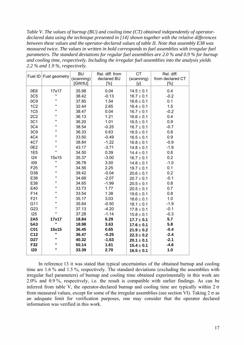
Table V. The values of burnup (BU) and cooling time (CT) obtained independently of operator-declared data using the technique presented in [14] shown together with the relative differences between these values and the operator-declared values of table II. Note that assembly E38 was measured twice. The values in written in bold corresponds to fuel assemblies with irregular fuel parameters. The standard deviations for regular fuel assemblies are 2.0 % and 0.9 % for burnup and cooling time, respectively. Including the irregular fuel assemblies into the analysis yields 2.2 % and 1.9 %, respectively.

Fuel ID

Fuel geometry

BU (scanning)

[GW/tU]

Rel. diff. from declared BU

[%]

CT (scanning)

[y]

Rel. diff. from declared CT

[%]

0E6 3C5 0C9 1C2 1C5 2C2 3C1 3C4 3C9 4C4 4C7 0E2 1E5 I24 I09 F25 D38 E38 E38 E40 F14 F21 G11 G23 I25 2A5 5A3 C01 C12 D27 F32 I20

17x17 " " " " " " " " " " " "

15x15 " " " " " " " " " " "

17x17 "

15x15 " " " "

35.98 38.42 37.85 32.44 38.47 36.13 36.20 38.54 36.33 33.50 38.84 43.17 34.50 35.37 38.78 34.56 39.42 34.68 34.65 33.73 33.54 35.17 35.64 37.13 37.28 18.84 18.98 36.45 36.47 40.32 50.14 33.39

0.04 -0.13 1.54 2.65 0.04 1.21 1.01 -0.25 0.63 -0.49 -1.22 -3.71 0.39 -3.00 3.50 2.25 -0.04 -2.07 -1.99 1.77 1.38 3.03 -0.50 -4.20 -1.14 6.29 3.63 0.65 -0.25 -1.63 1.61 2.70

14.5 ± 0.1 16.7 ± 0.1 16.6 ± 0.1 16.4 ± 0.1 16.7 ± 0.1 16.6 ± 0.1 16.5 ± 0.1 16.7 ± 0.1 16.5 ± 0.1 16.5 ± 0.1 16.8 ± 0.1 14.8 ± 0.1 14.4 ± 0.1 16.7 ± 0.1 14.8 ± 0.1 19.7 ± 0.1 20.6 ± 0.1 20.7 ± 0.1 20.5 ± 0.1 20.5 ± 0.1 19.6 ± 0.1 18.6 ± 0.1 18.1 ± 0.1 17.8 ± 0.1 15.8 ± 0.1 17.7 ± 0.1 17.6 ± 0.1 21.9 ± 0.2 22.3 ± 0.2 20.1 ± 0.1 15.4 ± 0.1 16.5 ± 0.1

0.4 -0.2 0.1 1.5 -0.2 0.4 0.9 -0.7 0.8 0.9 -0.9 -1.9 0.8 0.2 -1.0 0.1 0.2 -0.1 0.8 0.7 0.8 1.0 -1.9 -0.1 -0.3 5.7 5.8 -0.4 -2.4 -2.1 -4.6 1.0

In reference 13 it was stated that typical uncertainties of the obtained burnup and cooling

time are 1.6 % and 1.5 %, respectively. The standard deviations (excluding the assemblies with irregular fuel parameters) of burnup and cooling time obtained experimentally in this work are 2.0% and 0.9 %, respectively, i.e. the result is compatible with earlier findings. As can be inferred from table V, the operator-declared burnup and cooling time are typically within 2 σ from measured values, except for some of the irregular assemblies (see section VI). Taking 2 σ as an adequate limit for verification purposes, one may consider that the operator declared information was verified in this work.

17

V.C Verification of calculated decay heat, case (i) As the operator-declared burnup and cooling time were verified, these values could be used

in eq. (2.3) to obtain the fractional contribution f for each fuel assembly. The decay heat was then obtained by inserting into eq. (2.1) the calibration constants C of table III and the measured gamma-ray intensities of 137Cs, corrected for f. The resulting experimental values of the decay heat are shown in table VI together with the differences of the experimental decay heat from the values obtained in SNF calculations. It can be concluded from table IV that the relative standard deviation of the experimental decay heat from the calorimetric decay heat is 1.8 % or 2.3 %, depending on whether the irregular fuel assemblies are included in the analysis or not. This can be used as a direct measure of the uncertainty of the gamma-scanning data. The main contributor to the uncertainty (in the order of 2 %) is considered to be the estimation of the fractional contribution f, due to the highly general modelling of the power history, limitations in the parameterization of eq. (2.3) and on uncertainties in the input burnup.

Table VI. The results of the verification of the SNF calculations. The standard deviation of the relative difference between the gamma-ray measurements and the calorimetric measurements is 1.8 % without and 2.3 % with inclusion of the irregular assemblies. The calculated (SNF) values are verified within 1.8 % without and 2.3 % with inclusion of the irregular assemblies. Fuel ID

Fuel geometry

Decay heat (scanning)

[W]

Rel. diff. From calorimetry

[%]

Rel. diff. from SNF calculations

[%]

0E6 3C5 0C9 1C2 1C5 2C2 3C1 3C4 3C9 4C4 4C7 0E2 1E5 I24 I09 F25 D38 E38 E38 E40 F14 F21 G11 G23 I25 2A5 5A3 C01 C12 D27 F32 I20

17x17 " " " " " " " " " " " "

15x15 " " " " " " " " " " "

17x17 "

15x15 " " " "

481.5 500.0 493.1 415.5 499.5 467.5 469.5 500.6 470.8 427.9 503.8 587.2 460.0 420.4 488.4 389.8 446.4 383.3 384.8 373.6 377.6 406.7 413.6 434.7 455.9 224.3 228.0 397.8 394.8 459.7 649.0 396.4

1.3 0.3 -0.4 0.5 -0.1 -0.2 0.1 -0.7 -0.5 -1.4 -1.0 0.1 1.9 -2.5 3.8 1.7 -0.9 -2.1 -2.5 2.0 1.1 3.4 0.7 -3.3 -2.3 4.0 3.3 4.3 3.8 -0.8 6.2 1.7

0.6 -0.9 0.5 1.5 -1.0 0.4 0.1 -1.3 -0.2 -1.5 -1.8 -1.4 1.0 -5.0 4.5 0.8 -1.6 -2.9 -3.3 0.5 -0.1 1.6 -1.6 -4.8 -1.7 5.9 2.4 4.8 4.6 -2.2 5.6 0.1

18

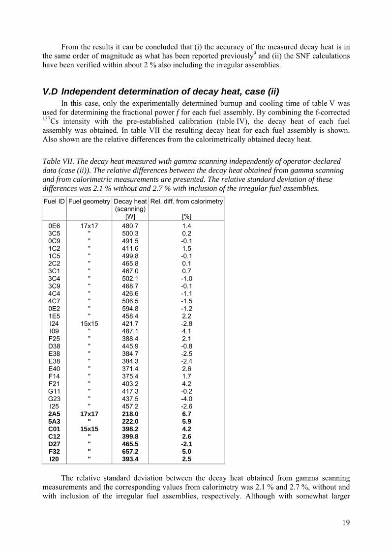
From the results it can be concluded that (i) the accuracy of the measured decay heat is in the same order of magnitude as what has been reported previously9 and (ii) the SNF calculations have been verified within about 2 % also including the irregular assemblies.

V.D Independent determination of decay heat, case (ii) In this case, only the experimentally determined burnup and cooling time of table V was

used for determining the fractional power f for each fuel assembly. By combining the f-corrected 137Cs intensity with the pre-established calibration (table IV), the decay heat of each fuel assembly was obtained. In table VII the resulting decay heat for each fuel assembly is shown. Also shown are the relative differences from the calorimetrically obtained decay heat.

Table VII. The decay heat measured with gamma scanning independently of operator-declared data (case (ii)). The relative differences between the decay heat obtained from gamma scanning and from calorimetric measurements are presented. The relative standard deviation of these differences was 2.1 % without and 2.7 % with inclusion of the irregular fuel assemblies. Fuel ID

Fuel geometry

Decay heat (scanning)

[W]

Rel. diff. from calorimetry

[%] 0E6 3C5 0C9 1C2 1C5 2C2 3C1 3C4 3C9 4C4 4C7 0E2 1E5 I24 I09 F25 D38 E38 E38 E40 F14 F21 G11 G23 I25 2A5 5A3 C01 C12 D27 F32 I20

17x17 " " " " " " " " " " " "

15x15 " " " " " " " " " " "

17x17 "

15x15 " " " "

480.7 500.3 491.5 411.6 499.8 465.8 467.0 502.1 468.7 426.6 506.5 594.8 458.4 421.7 487.1 388.4 445.9 384.7 384.3 371.4 375.4 403.2 417.3 437.5 457.2 218.0 222.0 398.2 399.8 465.5 657.2 393.4

1.4 0.2 -0.1 1.5 -0.1 0.1 0.7 -1.0 -0.1 -1.1 -1.5 -1.2 2.2 -2.8 4.1 2.1 -0.8 -2.5 -2.4 2.6 1.7 4.2 -0.2 -4.0 -2.6 6.7 5.9 4.2 2.6 -2.1 5.0 2.5

The relative standard deviation between the decay heat obtained from gamma scanning

measurements and the corresponding values from calorimetry was 2.1 % and 2.7 %, without and with inclusion of the irregular fuel assemblies, respectively. Although with somewhat larger

19

uncertainties compared to case (i), this result constitutes a measure of the ability to use the gamma scanning method as an independent system for measurements of decay heat.

VI Discussion In this work, the analysis has been tailored for fuel assemblies with regular fuel parameters,

and, accordingly, the calibration was performed only for such assemblies. Because irregularities can be of a large variety, taking such assemblies into account can be difficult. However, in this work seven assemblies with various irregular irradiation histories were included in order to obtain an estimation of the accuracy of the method in the general case.

From table V it can be inferred that the irregular fuel assemblies in general exhibit larger

deviations between declared and measured values of burnup and cooling time than the regular assemblies. Also, the measured burnup and cooling time are input for the determination of the decay heat and, therefore, the deviations will be transferred to the decay heat determination. This effect is, however, somewhat relaxed by the fact that the dependency of f on burnup and cooling time is relatively weak.

As shown in tables V, VI and VII, the results presented for most of the irregular assemblies

do not deviate much from the set of regular ones. The two assemblies that deviate the most in the current data set are 2A5 and 5A3, which belong to the first batch of fuel assemblies operated in the Ringhals 3 reactor. Taken into account that such fuel experienced a highly irregular history, it is not surprising that these assemblies deviate the most.

Finally, it should be noted that the vast majority of fuel assemblies in the inventory at CLAB exhibit regular fuel parameters. For these assemblies, gamma scanning constitutes a fast and reasonably accurate method for verifying decay heat. Also for assemblies exhibiting smaller irregularities in the irradiation history, the gamma scanning method can be useful, although, as has been reported here, with somewhat degraded precision.

VII SUMMARY The activities reported in this work are part of the project aimed at the development of an

integrated measurement system for the characterization of spent nuclear fuel assemblies at the proposed spent fuel encapsulation plant in Sweden. As part of the activities, data-acquisition and analysis software for a pilot gamma scanning system has been developed. Also, gamma-scanning measurements and calorimetric measurements of 31 spent PWR fuel assemblies have been analyzed. The measurements were performed at the CLAB facilities in Oskarshamn. In addition, the decay heat has also been calculated using Studsvik Scandpower's integrated supplement for back-end fuel cycle analysis, SNF.

The calorimetric measurements were used to obtain a calibration of the gamma-scanning system for application in the measurement of decay heat. The calibration procedure allowed us to investigate the ability of the gamma scanning method to be used either as an independent system for the measurement of decay heat or as a complement that can be used for verification of the calculated decay heat.

The results of the investigations showed that the correlation between decay heat and the gamma-ray intensity was established to within 2.3% (1 σ) using verified operator-declared burnup and cooling time. In this procedure, the calculated decay heat using SNF was verified

20

within 2.3% (1 σ). In addition, it was shown that the decay heat could be determined independently of operator-declared data within 2.7% (1 σ).

VIII OUTLOOK Only the PWR fuel assemblies that were reported in the SNF validation report were

accounted for in this paper. Calibration of the gamma scanning system will be performed for the other typical fuel geometries that will be handled at the encapsulation plant. In addition, more measurements will be performed in 2007, involving both calorimetry and gamma scanning. The aim of the measurements will be to evaluate the repeatability of the calorimetric measurements, cross validate the calibration of the gamma scanning system and to evaluate the normalization procedure between different gamma scanning measurements, which is necessary for cases that involves changes in the detector system and the measuring geometry.

To improve the technique, the following areas will be considered:

i) The gamma scanning system used in this work is a test system, not designed for precision measurements. Among other things, the long distance between fuel assembly and detector tends to increase the uncertainty in positioning and thus in the measured count rate. Also, the water contained between the assembly and the detector attenuates radiation, which causes unnecessary long measuring times in order to obtain adequate statistics for, especially, radiation from the short-lived 134Cs. It is therefore reasonable that a dedicated measuring system is constructed and built for the encapsulation facility.

ii) The use of gamma transport coefficients, as calculated with a technique used in tomographic computations20 to relate the calibration constants C for different fuel designs to each other. This would make it possible to construct one calibration curve for all fuel types. By using such gamma transport coefficients, it may be possible to handle the following cases: a) The determination of the decay heat for fuel designs that are too few to be used in

a calibration curve. b) The modeling and determination of the decay heat for reconstructed fuel

assemblies where fuel rods have been removed or replaced. Also spent PWR fuel assemblies containing control rods clusters could be included in the analysis.

c) The use of a single reference fuel assembly for calibration and normalization purposes.

iii) Improved precision in the verification of decay heat through improved modeling of the fractional power f to make full use of available data. Special attention to the irradiation history and its impact on the results can be envisaged. This, however, requires that such a parameter can be verified experimentally.

ACKNOWLEDGEMENT The Authors wishes to express their appreciation to Fredrik Sturek and other staff members

at CLAB, Lennart Agrenius (Agrenius Engineering), Per Grahn, Anders Nyström (the Swedish Nuclear Fuel and Waste Management Co, SKB) for their contributions in the acquisition of the calorimetric data used in this work. The contributions of Sigurd Børresten are also acknowledged for making the results of the SNF computations available for application in this work.

21

References 1. P-E. AHLSTRÖM, “Towards a Swedish repository for spent fuel,” Nucl. Eng. Des. 176,

67 (1997). 2. F. A. DONATH, “Postclosure Environmental Conditions and Waste Form Stability in a

Geologic Repository for High-level Nuclear Waste,” Nuclear and Chemical Waste Management, 1, 103 (1980).

3. H. RAIKKO, “Thermal Dimensioning of Repository and its Influence on Operation Time-Scale,” VTT Technical Research Centre, Finland (2004).

4. K. IKONEN, “Thermal Analyses of Spent Nuclear Fuel Repository,” Posiva report, POSIVA 2003-04, (2003). Retrieved from:http://www.posiva.fi/raportit/Posiva_2003-04.pdf.

5. B. DUCHEMIN, C. NORDBORG, “Decay Heat Calculation, An International Nuclear Code Comparison”, NEACRP-319, Nuclear Energy Agency, (1989). Retrieved from: http://www.nea.fr/html/science/docs/1989.

6. I. C. GAULD, “Decay Heat Code Validation Activities at ORNL: Supporting Expansion of NRC Regulatory Guide 3.54”, ANS winter meeting (2001). Retrieved from: http://www.ornl.gov/~webworks/cppr/y2001/pres/111200.pdf, January 27, 2007.

7. H. RAMTHUN, “Recent Developments in Calorimetric Measurements of Radioactivity,” Nucl. Instrum. Meth., 112, 265 (1973).

8. S. R. GUNN, “Radiometric Calorimetry: a Review,” Nucl. Instrum. Meth,. 29, 1 (1964). 9. P. JANSSON, A. HÅKANSSON, A. BÄCKLIN and S. JACOBSSON, “Gamma-ray

Spectroscopy Measurements of Decay Heat in Spent Nuclear Fuel,” Nuclear Science and Engineering ,141, 129 (2002).

10. P. JANSSON, “Studies of Nuclear Fuel by Means of Nuclear Spectroscopic Methods,” PhD Thesis, Uppsala University (2002).

11. F. STUREK and L. AGRENIUS, “CLAB measurements of decay heat in spent fuel assemblies,” Swedish Nuclear Fuel and Waste Management Co (2005).

12. S. BØRRESEN and M. KRUNERS, “Validation of SNF Against CLAB Decay Heat Measurements,” SSP-04/216, Studsvik Scandpower (2005).

13. C. WILLMAN, A. HÅKANSSON, O. OSIFO, A. BÄCKLIN and S. JACOBSSON SVÄRD, “Non-destructive assay of Spent Nuclear Fuel with Gamma-Ray Spectroscopy,” Annals of Nuclear Energy, 33, 427 (2006).

14. M. TARVAINEN, A. BÄCKLIN and A. HÅKANSSON, “Calibration of the TVO spent BWR reference fuel assembly,” STUK-YTO-TR 37, Finnish Centre for Radiation and Nuclear Safety (1992).

15. O. OSIFO, “Gamma scanning of spent nuclear fuel assemblies: determination of decay heat using new data acquisition and analysis software,” Project report, Swedish Nuclear Fuel and Waste Management Co, SKB (2005).

16. APTEC-NRC, “PCMCA/Super, Basic Display and Acquisition Software, Rev. 00”. 17. APTEC-NRC, “Detailed Software and Board Documentation, Rev. 07”. 18. APTEC-NRC, “Series 5000 MCArd, Rev. 01”, Hardware Manual. 19. APTEC-NRC, “PC BASED MCA CARDS For No-NIMS Spectroscopy”. 20. S. JACOBSSON SVÄRD, “A Tomographic Measurement Technique for Irradiated

Nuclear Fuel Assemblies,” PhD Thesis, Uppsala University (2004).

22