AUTOMATIC GENERATION OF NATURAL LANGUAGE SUMMARIES

AUTOMATIC GENERATION OF NATURAL

LANGUAGE SUMMARIES

Dimitrios Galanis

PH.D. THESIS

DEPARTMENT OF INFORMATICS

ATHENS UNIVERSITY OF ECONOMICS AND BUSINESS

2012

Abstract

Automatic text summarization has gained much interest in the last few years, since it

could, at least in principle, make the process of information seeking in large document

collections less tedious and time-consuming. Most existing summarization methods

generate summaries by initially extracting the sentences that are most relevant to the

user’s query from documents returned by an information retrieval engine.

In this thesis, we present a new competitive sentence extraction method that assigns

relevance scores to the sentences of the texts to be summarized. Coupled with a sim-

ple method to avoid selecting redundant sentences, the resulting summarization system

achieves state-of-the-art results on widely used benchmark datasets.

Moreover, we propose two novel sentence compression methods, which rewrite a

source sentence in a shorter form, retaining the most important information. The first

method produces extractive compressions, i.e., it only deletes words, whereas the sec-

ond one produces abstractive compressions, i.e., it also uses paraphrasing. Experi-

ments show that the extractive method generates compressions better or comparable, in

terms of grammaticality and meaning preservation, to those produced by state-of-the-

art systems. On the other hand, the abstractive method produces more varied (due to

paraphrasing) and slightly shorter compressions than the extractive one. In terms of

grammaticality and meaning preservation, the two methods have similar scores.

Finally, we propose an optimization model that generates summaries by jointly se-

ii

ABSTRACT iii

lecting the most relevant and non-redundant input sentences. Sentence relevance is es-

timated using our sentence extraction method, and redundancy is estimated by counting

how many word bigrams of the input sentences occur in the summary. Experimen-

tal evaluation with widely used datasets shows that the proposed optimization method

ranks among the top perfoming systems.

Acknowledgements

I would like to thank my parents Kostas and Eleftheria, as well as my sister Maria

for their continuous support all these years. I also want to thank three other family

members, Aris, Sofia and Panos for their help and positive attitude. A big thank you

goes to Christina for her incredible encouragement. I would never forget to thank all the

former and current members of AUEB’s Natural Language Processing Group for their

collaboration, and all friends, expecially Makis Malakasiotis and Makis Lampouras, for

their support. Finally, I would like to thank my supervisor Ion Androutsopoulos for his

help and support throughout the work of this thesis.

iv

Contents

Abstract ii

Acknowledgements iv

Contents v

1 Introduction 1

1.1 Motivation . . . . . . . . . . . . . . . . . . . . . . . . . . . . . . . . . 1

1.2 Contribution of this thesis . . . . . . . . . . . . . . . . . . . . . . . . . 2

1.3 Overview of the rest of this thesis . . . . . . . . . . . . . . . . . . . . 4

2 An Overview of Text Summarization 6

2.1 Introduction . . . . . . . . . . . . . . . . . . . . . . . . . . . . . . . . 6

2.2 State-of-the-art generation of summaries . . . . . . . . . . . . . . . . . 8

2.3 Evaluating the content and readability of summaries . . . . . . . . . . . 15

2.3.1 Manual evaluation . . . . . . . . . . . . . . . . . . . . . . . . 15

2.3.2 Automatic evaluations . . . . . . . . . . . . . . . . . . . . . . 17

2.3.2.1 ROUGE . . . . . . . . . . . . . . . . . . . . . . . . 17

2.3.2.2 Basic Elements . . . . . . . . . . . . . . . . . . . . 18

2.3.2.3 Other automatic evaluation measures . . . . . . . . . 19

v

CONTENTS vi

3 An Introduction to Machine Learning and ILP 21

3.1 Maximum Entropy classifier . . . . . . . . . . . . . . . . . . . . . . . 21

3.2 Support Vector Regression . . . . . . . . . . . . . . . . . . . . . . . . 23

3.3 Latent Dirichlet Allocation . . . . . . . . . . . . . . . . . . . . . . . . 24

3.4 Integer Linear Programming . . . . . . . . . . . . . . . . . . . . . . . 25

4 Sentence Extraction 27

4.1 Introduction and related work . . . . . . . . . . . . . . . . . . . . . . . 27

4.2 Our SVR model of sentence extraction . . . . . . . . . . . . . . . . . . 28

4.3 Preprocessing . . . . . . . . . . . . . . . . . . . . . . . . . . . . . . . 30

4.4 Experiments on DUC 2007 data . . . . . . . . . . . . . . . . . . . . . 31

4.5 Participation in TAC 2008: Official results and discussion . . . . . . . . 33

4.6 Generating summaries from blogs . . . . . . . . . . . . . . . . . . . . 36

4.7 Conclusions . . . . . . . . . . . . . . . . . . . . . . . . . . . . . . . . 39

5 Extractive Sentence Compression 41

5.1 Introduction . . . . . . . . . . . . . . . . . . . . . . . . . . . . . . . . 41

5.2 Related work . . . . . . . . . . . . . . . . . . . . . . . . . . . . . . . 43

5.3 Our method . . . . . . . . . . . . . . . . . . . . . . . . . . . . . . . . 46

5.3.1 Generating candidate compressions . . . . . . . . . . . . . . . 47

5.3.2 Ranking candidate compressions . . . . . . . . . . . . . . . . . 50

5.3.2.1 Grammaticality and importance rate . . . . . . . . . 50

5.3.2.2 Support Vector Regression . . . . . . . . . . . . . . 52

5.4 Baseline and T3 . . . . . . . . . . . . . . . . . . . . . . . . . . . . . . 53

5.5 Experiments . . . . . . . . . . . . . . . . . . . . . . . . . . . . . . . . 54

5.5.1 Experimental setup . . . . . . . . . . . . . . . . . . . . . . . . 55

5.5.2 Best configuration of our method . . . . . . . . . . . . . . . . 55

CONTENTS vii

5.5.3 Our method against T3 . . . . . . . . . . . . . . . . . . . . . . 57

5.6 Conclusions . . . . . . . . . . . . . . . . . . . . . . . . . . . . . . . . 59

6 Abstractive Sentence Compression 60

6.1 Introduction . . . . . . . . . . . . . . . . . . . . . . . . . . . . . . . . 60

6.2 Prior work on abstractive compression . . . . . . . . . . . . . . . . . . 62

6.3 The new dataset . . . . . . . . . . . . . . . . . . . . . . . . . . . . . . 64

6.3.1 Extractive candidate compressions . . . . . . . . . . . . . . . . 66

6.3.2 Abstractive candidate compressions . . . . . . . . . . . . . . . 66

6.3.3 Human judgement annotations . . . . . . . . . . . . . . . . . . 67

6.3.4 Inter-annotator agreement . . . . . . . . . . . . . . . . . . . . 70

6.3.5 Performance boundaries . . . . . . . . . . . . . . . . . . . . . 71

6.4 Our abstractive compressor . . . . . . . . . . . . . . . . . . . . . . . . 73

6.4.1 Ranking candidates with an SVR . . . . . . . . . . . . . . . . 73

6.4.2 Base form of our SVR ranking component . . . . . . . . . . . . 74

6.4.3 Additional PMI-based features . . . . . . . . . . . . . . . . . . 75

6.4.4 Additional LDA-based features . . . . . . . . . . . . . . . . . 76

6.5 Best configuration of our method . . . . . . . . . . . . . . . . . . . . . 77

6.6 Best configuration against GA-EXTR . . . . . . . . . . . . . . . . . . . 78

6.7 Conclusions and future work . . . . . . . . . . . . . . . . . . . . . . . 79

7 Generating Summaries using ILP 82

7.1 Introduction and related work . . . . . . . . . . . . . . . . . . . . . . . 82

7.2 Our models . . . . . . . . . . . . . . . . . . . . . . . . . . . . . . . . 86

7.2.1 Estimating sentence relevance using SVR . . . . . . . . . . . . 86

7.2.2 Baseline summarizers . . . . . . . . . . . . . . . . . . . . . . 88

7.2.3 Extractive ILP model . . . . . . . . . . . . . . . . . . . . . . . 88

CONTENTS viii

7.3 Datasets and experimental setup . . . . . . . . . . . . . . . . . . . . . 91

7.4 Best configuration of our models . . . . . . . . . . . . . . . . . . . . . 92

7.5 Our best configuration against state-of-the-art summarizers . . . . . . . 95

7.6 Conclusion . . . . . . . . . . . . . . . . . . . . . . . . . . . . . . . . 96

8 Conclusions 97

8.1 Sentence extraction . . . . . . . . . . . . . . . . . . . . . . . . . . . . 97

8.2 Extractive compression . . . . . . . . . . . . . . . . . . . . . . . . . . 98

8.3 Abstractive compression . . . . . . . . . . . . . . . . . . . . . . . . . 98

8.4 Summary generation . . . . . . . . . . . . . . . . . . . . . . . . . . . 99

8.5 Future work . . . . . . . . . . . . . . . . . . . . . . . . . . . . . . . . 99

A Abstractive Compression Annotation Guidelines 101

A.1 Guidelines . . . . . . . . . . . . . . . . . . . . . . . . . . . . . . . . . 101

Bibliography 104

Chapter 1

Introduction

1.1 Motivation

"Text Summarization is the process of distilling the most important information from one

or more texts to produce an abridged version for a particular task and user." (Section

23.3 of Jurafsky and Martin (2008))

High quality text summarization (TS) is very important, as it would improve search

in many applications. For example, today’s search engines often return hundreds if not

thousands of links to documents (Web pages, PDF files, etc.) when given a complex

natural language question or a set of several keywords. The users subsequently have

to read these documents to locate the information they need. This is a time-consuming

process which could, at least in princliple, be avoided by using an automatic TS system.

The system would have to be able to locate the most important and relevant to the query

information in the documents returned by a search engine, and generate an informative

and coherent summary.

1

CHAPTER 1. INTRODUCTION 2

1.2 Contribution of this thesis

Most current text summarization systems generate summaries by attempting to extract

(select) the most relevant (to a query) and non-redundant sentences from a set of input

documents. These sentences are either used verbatim or they are modified appropri-

ately. For example, they may be rewritten in a shorter form (sentence compression) in

order to discard their less informative parts and save space in the final summary; usu-

ally summaries are constrained to a maximum number words. Sentence compression is

usually perfomed by deleting words (extractive compression); however, in some more

recent approaches paraphrasing is also used (abstractive compression). There are also

methods that regenerate the referring expressions (e.g., pronouns) of the selected sen-

tences to resolve ambiguous references, and methods that order the selected sentences

to improve the summary’s coherence. Finally, there are methods that attempt to produce

more concise and fluent summaries by combining sentences into longer ones (sentence

fusion) that retain the most important information of the original ones. Relevant sum-

marization methods are presented in the following chapter.

Given this context, the contributions of this thesis to the area of automatic summa-

rization are the following.

Sentence Extraction: A new, competitive method to extract the most relevant sen-

tences of a document collection to be summarized has been developed. The method

assigns relevance (salience) scores to the input sentences using a Support Vector Re-

gression (SVR) model (Vapnik, 1998). In contrast to previous SVR-based sentence ex-

traction methods, the extraction method of this thesis uses an SVR trained on examples

whose target (ideal, to be predicted) scores are calculated using n-gram similarity mea-

sures (ROUGE-2 and ROUGE-SU4) that are broadly used for summary evaluation (Lin,

2004). There are also differences in the features used by the SVR of this thesis, com-


pared to previous SVR-based sentence extraction methods. Experimental evaluation has

shown that our model coupled with a simple method to avoid selecting redundant sen-

tences manages to generate summaries comparable to those produced by state-of-the-art

systems, when summarizing news articles and blog posts.

Extractive Sentence Compression: A novel method to generate extractive sentence

compressions has also been developed. It operates in two stages. In the first stage, mul-

tiple candidate compressions are produced by deleting branches from the dependency

tree of the source sentence. To limit the number of candidates, a trained Maximum En-

tropy classifier (Berger et al., 2006) is employed to reject unlikely actions (e.g., unlikely

branch deletions). In the second stage, an SVR model is used to select the best candidate

compression, in terms of grammaticality and meaning preservation using mostly syn-

tactic amd semantic features. Experimental evaluation of our extractive compression

method has shown that it generates comparable or better compressions, compared to

those of a state-of-the-art system.

Abstractive Sentence Compression: An additional novel method to generate abstrac-

tive compressions was also developed; unlike the previous method, it does not just

delete words. This method also operates in two stages. In the first stage, a large pool

of candidate sentence compressions is generated. This pool consists of (a) extractive

candidates, which are generated with our extractive compression method and (b) ab-

stractives candidates, which are generated by applying paraphrasing rules on the ex-

tractive candidates. In the second stage, the best candidates of the pool in terms of

grammaticality are kept and they are ranked using an SVR model to select the best one.

The feature set of this SVR includes language model scores, the confidence score of

the extractive sentence compressor, the number of paraphrasing rules that have been

applied, as well as features from word co-occurrence measures and Latent Dirichlet Al-

location models (Blei et al., 2003). In order to train and evaluate different possible con-


figurations of this method’s SVR, we constructed a new publicly available dataset that

contains extractive and abstractive candidates annotated with grammaticality and mean-

ing preservation scores provided by human judges. Experimental evaluation has shown

that our abstractive compressor generates more varied (because of the paraphrasing) and

slightly shorter sentence compressions, with negligible deterioration in grammaticality

and meaning preservation, compared to our extractive sentence compressor.

An Integer Linear Programming model (ILP) for generating summaries: This

model attempts to form a summary by selecting the most relevant sentences, avoiding at

the same time redundant sentences, i.e., sentences conveying similar information. Rel-

evance is estimated using the SVR of our earlier sentence extraction method; and non-

redundancy is estimated by counting how many different 2-grams of the original texts

occur in the summary. Following previous work on summarization (Berg-Kirkpatrick

et al., 2011), we assume that these 2-grams correspond to different concepts. Experi-

mental results show that our ILP model generates summaries that are better than those

produced by our earlier sentence extraction method coupled with simpler techniques to

avoid redundant sentences, and better than or comparable to the summaries produced

by top performing systems.

1.3 Overview of the rest of this thesis

Chapter 2 provides an overview of automatic text summarization. In particular, it

presents (a) the most important problems and concepts that are related to the task of

automatic summary generation, and (b) the methods that are currently used for sum-

mary evaluation. Chapter 3 provides a brief introduction to the machine learning and

optimization methods used in this thesis. Chapter 4 discusses the SVR-based sentence

extraction method of this thesis. Chapter 5 and 6 present the extractive and abstractive


sentence compression methods of this thesis, respectively. Chapter 7 is devoted to our

Integer Linear Programming model for summary generation. Chapter 8 concludes and

proposes directions for future research.

Chapter 2

An Overview of Text Summarization

2.1 Introduction

The first algorithms for text summarization (TS) were presented by Luhn (1958) and

Edmundson (1969). Several other approaches were presented in the following decades;

see chapter 23 of Jurafsky and Martin (2008). Kupiec et al.’s (1995) sentence extraction

method was the first among many others that followed which used machine learning or

statistical models to generate summaries. Such methods have dominated the last decade

in which there has been an increasing interest in TS due to to the information overload

of the World Wide Web. This interest is indicated by the fact that the National Institute

of Standards and Technology (NIST) 1 organized the annual Document Understand-

ing Conference series (DUC, 2001-2007) 2 and continues to organize the annual Text

Analysis Conference (TAC, 2008-2011). Both conferences series have focused on sum-

marization and have enabled the researchers to participate in large-scale experiments by

providing appropriate datasets.

1http://www.nist.gov/2http://duc.nist.gov/

6

CHAPTER 2. AN OVERVIEW OF TEXT SUMMARIZATION 7

Text summarization has been explored in texts of different genres and knowledge

domains, like news articles (Dang, 2005; Dang, 2006; Dang and Owczarzak, 2008;

Dang and Owczarzak, 2009), biomedical documents (Reeve et al., 2007), legal texts

(Moens, 2007), computer science papers (Mei and Zhai, 2008), blogs and reviews (Titov

and McDonald, 2008; Stoyanov and Cardie, 2006; Lloret et al., 2009) and more recently

short stories (Kazantseva and Szpakowicz, 2010). Each of these genres and domains

has different characteristics and therefore it is not easy to build a generic system that

would succesfully generate summaries in all of them. For example, in review and blog

summarization the target is to identify the positive and negative opinions of users (e.g.,

for products, companies, legislation, persons), whereas in the news domain the target

is to identify the pieces of text that convey the most important information for an event

(e.g., a bombing) . Therefore, in the former case systems may use lexicons which

contain words that express positive or negative sentiment (e.g., great restaurant, polite

bartender) (Blair-Goldensohn et al., 2008; Nishikawa et al., 2010b; Brody and Elhadad,

2010). By constrast, in the case of news documents such lexicons are typically not used;

instead frequency features on words may be used to detect the frequent pieces of text

since important information for a certain topic is likely to be repeated across a number

of related documents (Conroy et al., 2006; Galanis and Malakasiotis, 2008; Schilder

and Ravikumar, 2008; Toutanova et al., 2007).

Apart from their domain and gender or the techniques that are used to generate them,

summaries can also be classified as:

• Single or multi-document: Single document summaries are produced from one

document each, whereas a multi-document summary summarizes an entire cluster

of documents.

• Abstractive or extractive: Extractive summaries are formed by using a combina-


tion of sentences or parts of sentences of the source (input) documents in contrast

to abstractive summaries where sentences or parts of sentences of the source doc-

uments are reformulated by using different words and phrasings.

• Generic or query-focused: Generic summaries summarize the most important

points of the input document(s), while query-focused summaries attempt to an-

swer a user query.

2.2 State-of-the-art generation of summaries

The automatic generation of human-like (abstractive) summaries involves very difficult

tasks; for example, it requires deep understanding (interpretation) of the original texts

and reformulation (regeneration) of the content to be included in the summary, as it

is also noted by Kupiec et al. (1995), Sparck Jones (1999) and Murray et al. (2010).

The aforementioned tasks are very difficult and the methods that have been proposed to

address them can be used succesfully only in restricted domains (Kupiec et al., 1995;

Murray et al., 2010). An example of a restricted domain system that produces abstract

summaries of meeting conversations was presented by Murray et al. (2010). Initially,

the system maps the sentences of the conversations to a general meeting ontology, which

contains classes and properties pertaining to meetings. The mapping from sentences to

ontology instances is perfomed using several trained classifiers that, for example, map

parts of sentences to entities or classes of the ontology (e.g. meeting action or meeting

decision). The summary is then generated from the ontology and its instances using a

typical concept-to-text generation system (Reiter and Dale, 2000) that uses lexical re-

sources (e.g., noun phrases, phrase templates) associated with the entities and properties

of the ontology.


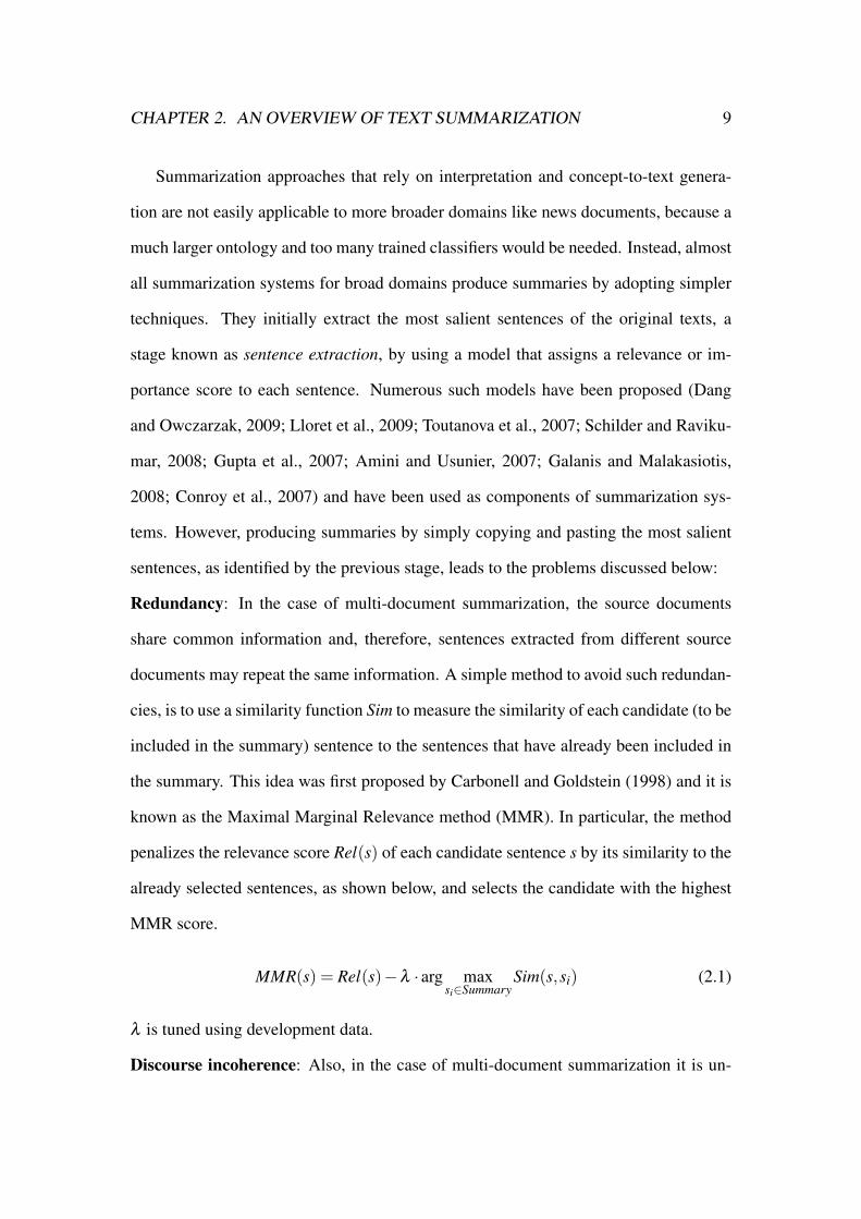
Summarization approaches that rely on interpretation and concept-to-text genera-

tion are not easily applicable to more broader domains like news documents, because a

much larger ontology and too many trained classifiers would be needed. Instead, almost

all summarization systems for broad domains produce summaries by adopting simpler

techniques. They initially extract the most salient sentences of the original texts, a

stage known as sentence extraction, by using a model that assigns a relevance or im-

portance score to each sentence. Numerous such models have been proposed (Dang

and Owczarzak, 2009; Lloret et al., 2009; Toutanova et al., 2007; Schilder and Raviku-

mar, 2008; Gupta et al., 2007; Amini and Usunier, 2007; Galanis and Malakasiotis,

2008; Conroy et al., 2007) and have been used as components of summarization sys-

tems. However, producing summaries by simply copying and pasting the most salient

sentences, as identified by the previous stage, leads to the problems discussed below:

Redundancy: In the case of multi-document summarization, the source documents

share common information and, therefore, sentences extracted from different source

documents may repeat the same information. A simple method to avoid such redundan-

cies, is to use a similarity function Sim to measure the similarity of each candidate (to be

included in the summary) sentence to the sentences that have already been included in

the summary. This idea was first proposed by Carbonell and Goldstein (1998) and it is

known as the Maximal Marginal Relevance method (MMR). In particular, the method

penalizes the relevance score Rel(s) of each candidate sentence s by its similarity to the

already selected sentences, as shown below, and selects the candidate with the highest

MMR score.

MMR(s) = Rel(s)−λ · arg maxsi∈Summary

Sim(s,si) (2.1)

λ is tuned using development data.

Discourse incoherence: Also, in the case of multi-document summarization it is un-


likely that the extracted sentences will form a coherent and readable text if presented

in an arbitrary order. Barzilay et al. (2002) have shown that sentence ordering affects

text readability and comprehension. To tackle this problem, several ordering algorithms

have been proposed (Barzilay et al., 2002; Lapata, 2003; Althaus et al., 2004; Bollegala

et al., 2005; Bollegala et al., 2006; Karamanis et al., 2009) which operate, however,

independently to sentence extraction. This may lead to situations where no appropriate

ordering of the extracted sentences exists. Recently, a joint algorithm that simultane-

ously extracts and orders sentences was proposed (Nishikawa et al., 2010b), and its

experimental evaluation showed that it generates more informative and readable sum-

maries of reviews than a baseline system with independent extraction and ordering. It is

worth noting that the sentence ordering problem has been shown (Althaus et al., 2004)

to correspond to the Travelling Salesman Problem (TSP) which is NP-hard. There-

fore, the task of finding the optimal sentence ordering is considered intractable for large

number of sentences. Furthermore, there are no good approximation algorithms for

TSP (Papadimitriou and Steiglitz, 1998), i.e., polynomial complexity algorithms which

find a near-optimal solution. 3

Uninformative content: There are often parts of the selected (extracted) sentences that

convey unimportant information or information irrelevant to the user’s query (when

there is one). This leads to unnatural summaries which do not convey the maximum

possible information, as space is wasted. Some summarization systems use sentence

compression algorithms to tackle this problem. Sentence compression is the task of

producing a shorter form of a grammatical source (input) sentence, so that the new form

will still be grammatical and it will retain the most important information of the source.

(Jing, 2000). Today, most sentence compression methods are extractive, meaning that

3Approximation algorithms have a proven approximation ratio which is a lower bound on the value

of the solutions the algorithm returns.


they form sentences by only deleting words. Abstractive sentence compression algo-

rithms, however, which are also capable of paraphrasing the source sentences, rather

than just deleting words, have also been proposed (Cohn and Lapata, 2008; Ganitke-

vitch et al., 2011). Published experimental results indicate that summarization systems

that used extractive compression to avoid uninformative content (Zajic, 2007; Gillick

and Favre, 2009; Conroy et al., 2007; Madnani et al., 2007) managed to include more

relevant information in the summaries. However, the linguistic quality (grammaticality)

scores of the summaries were seriously affected in a negative way (Gillick and Favre,

2009; Zajic et al., 2006; Madnani et al., 2007) due to the grammatical errors introduced

by sentence compression. Recently, a joint extractive sentence compression and sen-

tence extraction system was proposed (Berg-Kirkpatrick et al., 2011) that overcame this

problem, i.e., it produced more informative summaries than a non-compressive version

of the same system without (significant) loss of linguistic quality. An example summary

generated by the system of Berg-Kirkpatrick et al. (2011) is shown in Table 2.1.

Inappropriate sentence realisation: Another problem is that the sentences selected

for inclusion in the summary may not be appropriately realized, since they are taken

from different contexts.

For example, it is very likely that referring expressions (e.g., to objects or people)

may not be appropriate, affecting the summary’s readability. This was pointed out,

for example by Nenkova and McKeown (2003), who also proposed an algorithm that

rewrites referring expressions. The algorithm initially uses a coreference resolution sys-

tem, which attempts to find which noun phrases refer to the same entity (e.g., person).

A set of rewrite rules is then applied to revise apropriatelly the referring expressions.

An example of effects of Nenkova and McKeown (2003)’s algorithm is illustrated in

Table 2.2.

Moreover, in multi-document summarization it is useful to combine (fuse) sentences


The country’s work safety authority will release the list of the

first batch of coal mines to be closed down said Wang Xianzheng,

deputy director of the National Bureau of Production Safety Super-

vision and Administration. With its coal mining safety a hot issue,

attracting wide attention from both home and overseas, China is seek-

ing solutions from the world to improve its coal mining safety system.

Despite government promises to stem the carnage the death toll in China’s

disaster-plagued coal mine industry is rising according to the latest statistics

released by the government Friday. Fatal coal mine accidents in China rose

8.5 percent in the first eight months of this year with thousands dying despite

stepped-up efforts to make the industry safer state media said Wednesday.

Table 2.1: Example extractive summary produced by Berg-Kirkpatrick’s system. The

summary was generated from a cluster of source documents of TAC 2008. The parts of

the sentences that have been removed using sentence compression are underlined.


Original summary: Presidential advisers do not blame O’Neill, but they’ve

long recognized that a shakeup of the economic team would help indicate Bush

was doing everything he could to improve matters. U.S. President George W.

Bush pushed out Treasury Secretary Paul O’Neill and top economic adviser

Lawrence Lindsey on Friday, launching the first shake - up of his administra-

tion to tackle the ailing economy before the 2004 election campaign.

Rewritten summary: Presidential advisers do not blame Threasury Secre-

tary Paul O’Neill, but they’ve long recognized that a shakeup of the economic

team would help indicate U.S. President George W. Bush was doing every-

thing he could to improve matters. Bush pushed out O’Neill and White House

economic adviser Lawrence Lindsey on Friday, launching the first shake-up

of his administration to tackle the ailing economy before the 2004 election

campaign.

Table 2.2: Rewriting summary’s references using Nenkova’s algorithm.


in order to produce more fluent and concise text. Sentence fusion may involve deleting

unimportant parts of the sentences and/or reformulating (paraphrasing) their important

parts to form a more concise text. A human-created fusion of two sentences is given

in Table 2.3; the example is taken from Jing (1999)’s work. The first sentence fusion

algorithms were proposed by Jing (2000) and Barzilay and McKeown (2005). Several

other fusion algoritms followed (Filippova and Strube, 2008; Elsner and Santhanam,

2011). For example, Barzilay and McKeown (2005)’s algorithm parses the input sen-

tences and finds parts of them that convey the same information. A word lattice is then

contructed that contains the common information of the sentences, and finally a path of

words from this lattice is selected to form the fused sentence.

Sentence 1: But it also raises serious questions about the privacy of such

highly personal information wafting about the digital world.

Sentence 2: The issue thus fits squarely into the broader debate about

privacy and security on the internet, whether it involves protecting credit

card number or keeping children from offensive information.

Merged sentence: But it also raises the issue of privacy of such personal in-

formation and this issue hits the head on the nail in the broader debate about

privacy and security on the internet.

Table 2.3: Example of sentence fusion. The bold parts of the two input sentences are

those which are fused in the final sentence.


2.3 Evaluating the content and readability of summaries

2.3.1 Manual evaluation

In the DUC and TAC conferences, summaries are evaluated manually by a number of

NIST assessors. Each summary is judged by one assessor, the same one who created

the corresponding cluster of documents being summarized. Each cluster contains doc-

uments related to a specific topic, specified by a query. The summary is assigned one

score for content responsiveness, i.e, how well it answers the query, and five scores for

five linguistic quality measures, which measure its readability (Dang, 2006). All scores

are on scale of 1-5 (Very Poor, Poor, Barely Acceptable, Good, Very Good). The five

linguistic quality measures are presented below and were taken from (Dang, 2006).

• Grammaticality: The summary should have no datelines, system-internal format-

ting, capitalization errors or obviously ungrammatical sentences that make the

text difficult to read.

• Non-redundancy: There should be no unnecessary repetition in the summary. Un-

necessary repetition might take the form of whole sentences that are repeated, or

repeated facts, or the repeated use of a noun or noun phrase (e.g., “Bill Clinton”)

when a pronoun (“he”) would suffice.

• Referential-clarity: It should be easy to identify who or what the pronouns and

noun phrases in the summary refer to. If a person or other entity is mentioned, it

should be clear what their role in the story is. So, a reference would be unclear if

an entity is referenced but its identity or relation to the story remains unclear

• Focus: The summary should have a focus; sentences should only contain infor-

mation that is related to the rest of the summary.


• Structure and Coherence: The summary must be well-structured and well-organized.

The summary should not just be a heap of related information, but it should build

from sentence to sentence to a coherent body of information about a topic.

After judging them for readability (linguistic quality) and content responsiveness

the summaries are assigned a separate score by the judges which indicates each sum-

mary’s overall responsiveness (based on both content and readability). The latter scores

are assigned without the assessors knowing the previous two scores (for content and

readability).

Another method for summary evaluation, called the Pyramid method, was pro-

posed by Nenkova and Passonneau (2004). It is based on Summarization Content Units

(SCU), which are defined by Nenkova and Passonneau (2004) as “sub-sentential con-

tent units not bigger than a clause”. SCUs are constructed by manually annotating the

model (gold, human-written) summaries which are given for each topic. Each SCU has

a weight, which indicates how many summaries the SCU it appears in. After manual

annotation, SCUs are organized into a pyramid which consists of as many layers as the

number of model summaries. Each layer contains only the SCUs of the same weight,

for example, the bottom layer contains the SCUs with weights of 1. The top layers con-

tain the most important SCUs. Therefore, the optimal summary should contain all the

SCUs of the top layer and all the SCUs of the next layer, and so on up to a maximum

depth that corresponds to the size available for the summary. The score of the evaluated

summary is the ratio of the sum of the weights of its SCUs to the sum of weights of an

optimal summary with the same number of SCUs.


2.3.2 Automatic evaluations

NIST uses also three automatic evaluation measures: ROUGE-2, ROUGE-SU4, and Basic

Elements Head-Modifier (BE-HM) (Lin, 2004; Hovy et al., 2005). These measures are

also used by researchers to tune their systems in the development stage and to quickly

evaluate their systems against previous approaches.

2.3.2.1 ROUGE

ROUGE (Recall-Oriented Understudy for Gisting Evaluation) counts the number of

overlapping units (such as n-grams, word sequences, and word pairs) between an auto-

matically constructed summary and a set of reference (human) summaries. Lin (2004)

proposed four different measures: ROUGE-N, ROUGE-S, ROUGE-L, and ROUGE-W.

ROUGE-N is an n-gram recall between an automatically constructed summary S and

a set of reference summaries Refs .It is computed as follows:

ROUGE-N(S|Re f s) =∑R∈Refs ∑gn∈RC(gn,S,R)

∑R∈Refs ∑gn∈RC(gn,R)(2.2)

where gn is an n-gram, C(gn,S,R) is the number of times that gn co-occurs in S and

reference R, and C(gn,R) is the number of times gn occurs in reference R.

ROUGE-S measures the overlap of skip-bigrams between a candidate summary and

a set of reference summaries. A skip-bigram is any pair of words from a sentence, in

the same order as in the sentence, allowing for arbitrary gaps between the two words.

One problem with ROUGE-S is that it does not give any credit to a candidate summmary

if it does not have any word pair that also co-occurs in the reference summaries, even

if the candidate summmary has several individual words that also occur in the refer-

ence summaries. To address this problem ROUGE-S was extended to count unigrams

(individual words) that occur both in the candidate summary and the references. The

extended version is called ROUGE-SU.


The DUC and TAC conferences and most published papers use ROUGE-2 and ROUGE-

SU4 as evaluation measures, because they correlate well with human judges (Lin, 2004).

ROUGE-2 is ROUGE-N with N=2 and ROUGE-SU4 is a version of ROUGE-SU where the

maximum distance between the words of any skip-bigram is limited to four. The other

two aforementioned versions of ROUGE, i.e., ROUGE-L and ROUGE-W, are based on the

longest common subsequence between two sentences; however, ROUGE-W gives more

credit when the matches are consecutive.

2.3.2.2 Basic Elements

Basic Elements (BEs) are minimal “semantic units” which are appropriate for summary

evaluation (Hovy et al., 2005). More precisely, after a number of experiments, Hovy et

al. (2005) defined BEs as:

• the heads of major syntactic constituents (noun, verb, adjective, or adverbial

phrases) and

• the dependency grammar relations between a head and a single dependent, ex-

pressed as a triple < head, modifier, relation >.

The BEs evaluation process creates for each topic a list of BEs from the correspond-

ing human summaries. The elements of the list are then matched to the BEs of the

summary being evaluated. From this comparison, a resulting score is computed. More

specifically, the BE procedure uses the following modules:

• BE breaker module: This module takes a sentence as input and produces a list of

the sentence’s BEs as output. To produce BEs, several alternative techniques can

be used. Most of them use a syntactic parser and a set of “cutting rules” to extract

BEs from the parse tree of the sentence. Hovy et al. (2005) and Hovy et al. (2006)


experimented with Charniak’s parser (BE-L), the Collins parser (BE-Z), Minipar

(BE-F), and Microsoft’s parser, along with a different set of “cutting rules” for

each of them.

• Matching module: Several different approaches have been proposed to match the

BEs of the summary being evaluated to the ranked list that contains the BEs of the

reference summaries. Some of them are:

– lexical identity: The words must match exactly.

– lemma identity: The lemmata (base) forms of the words of the BE must

match.

– synonym identity: The words or any of their synonyms match.

– approximate phrasal paraphrase matching.

The default approach is lexical identity matching. The matching of BEs of the

form < head, modifier, relation > may or may not include the matching of their

relations. For each BE of the summary being evaluated that matches a BE of a

reference summary, the summary being evaluated receives one point. This point is

weighted depending on the completeness (relation matched or not) of the match.

The final score of the summary being evaluated is (simply) the sum of weighted

points it has received.

2.3.2.3 Other automatic evaluation measures

More recently, some new more sophisticated methods for automatic summary evalua-

tion were proposed (Giannakopoulos et al., 2009; Owczarzak, 2009; Tratz and Hovy,

2008) which achieve correlations with human judgements that are comparable or better

than those of ROUGE and BE. However, these methods have not been widely adopted


so far, because they are more complex than ROUGE (e.g. Owczarzak (2009)’s method

requires a dependency parser) and/or their correlation with human judgements is only

slightly better than the correlation of other previous automatic evalution measures.

Chapter 3

A brief Introduction to Machine

Learning and Integer Linear

Programming

In this chapter, we briefly describe some well known machine learning and optimization

methods that are used in this thesis: the Maximum Entropy classifier, Support Vector

Regression, Latent Dirichlet Allocation and Integer Linear Programming optimization.

3.1 Maximum Entropy classifier

A Maximum Entropy (ME) classifier (Berger et al., 2006) classifies each instance Y

described by its feature vector~x = 〈 f1, . . . , fm〉 to one of the classes of C = {c1, . . . ,ck}

by using the following learned distribution:

P(c|~x) =exp(∑m

i=1 wc,i fi)

∑c′∈C exp(∑

mi=1 wc′,i fi

)

21

CHAPTER 3. AN INTRODUCTION TO MACHINE LEARNING AND ILP 22

Y is is classified to the class c with the highest probability.

c = argmaxc∈C

P(c|~x)

wc,i is the weight of feature fi when we calculate the probability for class c, i.e., the

classifier learns a different feature weight for fi per class c.

To train an ME model, i.e., to learn the wc,i weights, we can maximize the conditional

likelihood of the training data. Assuming that we are given n training examples (~xi,yi)

where~xi is a feature vector and yi is the correct class of the i-th example, the conditional

likelihood of the training data is:

L(~w) = P(y1, . . . ,yn|~x1, . . . ,~xn) (3.1)

If we assume that training instances are independent and identically distributed, then

we can write the above formula as follows:

L(~w) =n

∏i=1

P(yi|~xi) (3.2)

Instead of maximizing equation 3.2 it is easier to maximize logL(~w):

~w∗ = argmax~w

logL(~w) = argmax~w

n

∑i=1

logP(yi|~xi) (3.3)

The optimal ~w∗ can be found using, for example, Gradient Ascend; see Manning et al.

(2003) for details. In practice, the ME model presented above may overfit the train-

ing data leading to poor generalisation (prediction accuracy) on unseen instances. To

address this problem, a bias (smoothing) factor is usually added as below to bias the

model towards ~w vectors that assign small (or zero) weights to many features.

~w∗ = argmax~w

n

∑i=1

logP(yi|~xi)−α

N

∑j=1

w2j (3.4)

For a more detailed introduction to ME models consult chapter 6 of Jurafsky and Martin

(2008).


3.2 Support Vector Regression

A Support Vector Regression (SVR) model aims to learn a function f : Rn→ R, which

will be used to predict the value of a continuous variable Y ∈R given a feature vector~x

In particular, given l training instances (~x1,y1), . . . ,(~xl,yl) where ~xi ∈ Rn are the

feature vectors and yi ∈R is a target real-valued score, an SVR model is learnt by solving

the following optimization problem (Vapnik, 1998); ~w is a vector of feature weights and

φ is a function that maps feature vectors to a higher dimensional space to allow non-

linear functions to be learnt in the original space. C > 0 and ε > 0 are given.

min~w,b,~ξ ,~ξ ∗

12‖~w‖2 +C

l

∑i=1

ξi +Cl

∑i=1

ξ∗i (3.5)

subject to:

~w ·φ(~xi)+b− yi ≤ ε +ξi,

yi−~w ·φ(~xi)−b≤ ε +ξ∗i ,

ξi ≥ 0,ξ ∗i ≥ 0,

i = 1, . . . , l

The purpose of the previous formulas is to learn an SVR model whose prediction ~w ·

φ(~xi)+ b for each training instance ~xi will not to be farther than ε from the target yi.

However, because this is not always feasible two slack variables ξi and ξ ∗i are used to

measure the prediction’s error above or below the target (correct) yi. The objective 3.5

minimizes simultaneously the total prediction error as well as ‖~w‖. The latter is used to

avoid overfitting as in the ME models.

The optimization problem is hard due to the (possible) high dimensionality of ~w. To

solve it, the primal form of the optimization problem 1 is transformed to a Langrangian

1the original form of the optimization problem


dual problem which is solved using a Sequential Minimal Optimization method (Chang

and Lin, 2001). The learnt function, which can be used to predict the y value of an

unseen instance described by feature vector~x, is the following:

f (~x) =l

∑i=1

(−ai +a∗i ) ·φ(~xi) ·φ(~x)+b = (3.6)

l

∑i=1

(−ai +a∗i ) ·K(~x,~xi)+b (3.7)

where ai, a∗i and b are learnt during optimization. K(~x,~xi) is a kernel function which ef-

ficiently computes the inner product φ(~xi) ·φ(~x) in the higher dimensionality space that

φ maps to, without explicitly computing φ(~xi) and φ(~x), as in Support Vector Machines

(Vapnik, 1998).

3.3 Latent Dirichlet Allocation

Latent Dirichlet Allocation (LDA) (Blei et al., 2003) is a probabilistic Bayesian model

of text generation which is based on prior work on Latent Semantic Indexing (LSI)

(Deerwester et al., 1990; Hofmann, 1999). LDA assumes that each document collec-

tion is generated for a mixture of K topics, and that each document of the collection

discusses these K topics to a different extent. It is worth noting that LDA is a bag-

of-words model, i.e., it assumes that word order within documents is not important.

Training an LDA model on a (large) document collection for a given, predefined

number of topics K amounts to learning a) the word-topic distribution P(w|t), and b)

the topic-document distribution P(t|d), i.e., to what extent the K topics are discussed in

each document d. Various methods have been proposed to learn these distributions such

as variational inference (Blei et al., 2003) and Gibbs Sampling (Steyvers and Griffiths,

2007). Table 3.1 illustrates the word-topic distribution P(w|t) for three topics (from


topic 247 topic 5 topic 43

DRUGS .069 RED .202 MIND .081

DRUG .060 BLUE .099 THOUGHT .066

MEDICINE .027 GREEN .096 REMEMBER .064

EFFECTS .026 YELLOW .073 MEMORY .037

BODY .023 WHITE .048 THINKING .030

Table 3.1: Examples of 3 topics learnt from a corpus of documents using LDA.

a total of 300); as they were learnt from a corpus of documents; the example is from

(Steyvers and Griffiths, 2007). For each topic, only the five words with the highest

P(w|t) are shown.

Given a trained LDA model and an unseen document dnew we can predict its topic

distribution P(t|dnew) using similar inference methods as before (Blei et al., 2003;

Steyvers and Griffiths, 2007) but keeping the word-topic distribution as it was esti-

mated during training. We we can also predict the probability of encountering a word

w in dnew using the following formula.

P(w|dnew) = ∑t

P(w|t) ·P(t|dnew) (3.8)

3.4 Integer Linear Programming

Linear Programming (LP) is a method to optimize (maximize or minimize) a linear

objective function subject to linear equality and inequality constraints. The variables

used in an LP formulation are called decision variables, and the target is to find the

values of decision variables that give the optimal objective value (Papadimitriou and

Steiglitz, 1998). More formally, a linear programming problem in its standard form is


specified as follows; see details in chapter 29 of Cormen et al. (2001):

z = cT · x (3.9)

subject to:

A · x≤ b,

x≥ 0

where x ∈Rn is the vector of decision variables, c ∈Rn, A is an m ·n real-valued matrix

and b ∈ Rm. The target is to optimize z.

Integer linear programming (ILP) problems are a special case of LP problems, where

all the decision variables are constrained to be integers. Unlike LP problems with real-

valued desision variables which can be solved in polynomial time, ILP problems are NP-

hard. The Mixed ILP problem, where only some variables are required to be integers,

is also NP-hard, and the same applies to the 0-1 ILP problem, where all variables are

required to be 0 or 1. Techniques that are used to solve efficiently the ILP problems

include Branch-and-Bound and Branch-and-Cut; both methods guarantee finding an

optimal solution.

Chapter 4

Sentence Extraction 1

4.1 Introduction and related work

Most current summarization systems produce summaries by extracting, at least initially,

the most salient sentences of the original documents. In earlier systems, the salience of

each sentence was usually calculated using a weighted linear combination of features,

where the weights were either assigned by experience or by a trial and error process.

More recently, regression models, for example Support Vector Regression (SVR Sec-

tion 3.2) have been used to combine these features, yielding very satisfactory results.

For example, Li et al. (2007) trained an SVR model on past DUC data documents. In

particular, for every sentence of the documents, one training vector was constructed by

calculating: a) some predetermined features and b) a label (a score) which indicates the

similarity of the sentence to sentences in the corresponding gold (reference) summaries

that were constructed by DUC’s judges. The trained SVR model was used to determine

the informativeness of each sentence (how much useful information it carries) and its

relevance to a given complex query. In DUC 2007, Li et al. (2007)’s system ranked 5th in

1Part of the work presented in this chapter has been published in (Galanis and Malakasiotis, 2008).

27

CHAPTER 4. SENTENCE EXTRACTION 28

ROUGE-2 and ROUGE-SU4, and 15th in content responsiveness among 32 participants.

2

Schilder and Ravikumar (2008) adopt a very similar approach with simple features

and a score which is calculated as the word overlap between the sentence that was

extracted from a document and the sentences in DUC’s summaries. Their results are

very satisfactory; as they ranked 6th and 2nd in ROUGE-2 in DUC 2007, and 2006

respectively.

We propose a different way to assign a score to each training example. We use

a combination of the ROUGE-2 and ROUGE-SU4 scores (Lin, 2004), because these

scores have strong correlation with the content responsiveness scores assigned by hu-

man judges and measures the information coverage of the summaries. Indeed, exper-

imental results, presented below, show that these scores allow our system to perform

very well. We also experiment with different sizes of training sets.

Our sentence extraction models were constructed aiming to generate summaries in

response to a complex user query, also taking as input a number of relevant documents

that were returned by a search engine for that query. Examples of such queries from the

DUC 2006 news summarization track are given below:

4.2 Our SVR model of sentence extraction

Our SVR-based sentence extraction uses the following features:

• Sentence position SP(s):

SP(s) =position(s,d(s))

|d(s)|

2NIST did not carry out an evaluation for overall responsiveness in DUC 2007 (Conroy and Dang,

2008).


topic id query

D0610A What are the advantages and disadvantages of home schooling? Is the

trend growing or declining?

D0617H What caused the crash of EgyptAir Flight 990? Include evidence, theo-

ries and speculation.

D0622D Track the spread of the West Nile virus through the United States and

the efforts taken to control it.

Table 4.1: Examples of topics taken from the DUC 2006 summarization track.

where s is a sentence, position(s,d(s)) is the position (sentence order) of s in its

document d(s), and |d(s)| is the number of sentences in d(s).

• Named entities NE(s):

NE(s) =n(s)

len(s)

where n(s) is the number of named entities in s and len(s) is the number of words

in s.

• Levenshtein distance LD(s,q): The Levenshtein Distance (Levenshtein, 1966)

between the query (q) and the sentence (s) counted in words.

• Word overlap WO(s, q): The word overlap (number of shared words) between the

query (q) and the sentence (s), after removing stop words and duplicate words.

• Content word frequency CF(s) and document frequency DF(s) as they are de-

fined by Schilder and Ravikumar (2008). In particular, CF(s) is defined as fol-

lows:

CF(s) =∑

csi=1 pc(wi)

cs


where cs is the number of content words in sentence s, pc(w) = mM , m is the

number of occurrences of the content word w in all input documents, and M is

the total number of content word occurences in the input documents. Similarly,

DF(s) is defined as follows:

DF(s) =∑

csi=1 pd(wi)

cs

where pd(w) = dD , d is the number of input documents the content word w occurs

in, and D is the number of all input documents.

Our SVR model of sentence extraction was trained on the DUC 2006 documents. All

the sentences of all the documents were extracted, and a training vector was constructed

for each one of them, containing the aforementioned 6 features. 3 The score which was

assigned to each training vector was calculated as the average of the ROUGE-2 and

ROUGE-SU4 of the sentence with the corresponding four model summaries.

4.3 Preprocessing

All training and test sentences were first compressed by using simple heuristics. Specif-

ically, the strings “However ,” , “In fact” , “At this point ,”, “As a matter of fact ,” , “,

however ,” and , “also ,” were deleted, as were some temporal phrases like “here today”

and “Today”. In addition, a small set of cleanup rules was used to remove unnecessary

formatting tags present in the source documents.

3We use LIBSVM (http://www.csie.ntu.edu.tw/ ∼cjlin/libsvm) with an RBF ker-

nel.


4.4 Experiments on DUC 2007 data

To evaluate our SVR model, we used it to construct summaries for the 45 sets of news

documents (clusters) that were given in DUC 2007. As in DUC 2006, each summary

had to be generated taking into account a complex user query. We used our SVR model,

trained on DUC 2006 data, to assign relevance scores to all the sentences of each cluster

of DUC 2007 data, and we used the resulting scores to sort the sentences of each clus-

ter. Starting from the sentence with the highest score, we added to the summary every

sentence whose similarity to each sentence already in the summary did not exceed a

threshold. 4 The similarity was measured using cosine similarity (over tokens) and the

threshold was determined by experimenting on DUC 2007 data. i.e., we used the DUC

2007 data as development set.

cos(~v,~w) =~v ·~w|v| · |w|

=∑

Ni=1 vi ·wi√

∑Ni=1 v2

i ·√

∑Ni=1 w2

i

(4.1)

In equation above~v and ~w are N-dimensional vectors; and vi and wi are binary variables

indicating if the i-th word of the vocabulary occurs in the sentences represented by ~v

and ~w, respectively.

Finally, the summaries that were generated were truncated by keeping their first 250

words, which was the maximum allowed size in DUC 2007. The best configuration of

our system achieved 0.113 in ROUGE-2 and 0.165 in ROUGE-SU4, being 5th in both

rankings among the 32 participants of DUC 2007. These scores were higher than those

of previous SVR-based systems (Li et al., 2007; Schilder and Ravikumar, 2008); see

Table 4.2.

We also experimented with different sizes of the training set (DUC 2006 data). The

results of these experiments are presented in Table 4.3, which shows that our summa-4The SVR-based summarizers of Li et al. (2007) and Schilder and Ravikumar (2008) also employ

similar methods for redundancy removal.


system ROUGE-2 ROUGE-SU4

Li et al. (2007) 0.111 0.162

Schilder and Ravikumar (2008) 0.110 N/A

Our SVR-based summarizer 0.113 0.165

Table 4.2: Comparison of our SVR-based summarizer against previous SVR-based mod-

els on DUC 2007 data.

rizer achieves its best results when it is trained with all of the available training exam-

ples. In these experiments, we did not use all the compression heuristics and cleanup

rules, which is why the ROUGE scores when using all the training data are worse that

those reported in Table 4.2.

training vectors ROUGE-2 ROUGE-SU4

35000 0.10916 (6th) 0.15959 (10th)

22000 0.10769 (9th) 0.15892 (10th)

11000 0.10807 (8th) 0.15835 (12th)

1000 0.10077 (16th) 0.15017 (18th)

10 0.10329 (13th) 0.15313 (16th)

2 0.06508 (30th) 0.11731 (31th)

Table 4.3: Our system’s ROUGE scores for different sizes of training datasets. The

system is trained on DUC 2006 data and it tested on DUC 2007 data.


4.5 Participation in TAC 2008: Official results and dis-

cussion

The UPDATE TASK in TAC 2008 was to produce summaries for 48 complex queries

provided by the organizers. For each query, two sets of news documents (set A and

B) were provided and the task was to produce two summaries, each one containing a

maximum of 100 words. The first summary should summarize the documents contained

in set A, and the second summary the documents contained in set B given that the reader

has already read the set A.

We produced the summary of each set A (for each query) using the summarizer that

was described in the previous section. For the summary of each set B, we used the same

summarizer, but we rejected the sentences with high similarity to any of the sentences

of corresponding set A. We used the same cosine similarity and threshold as before.

Each participating team was allowed to submit up to three runs, i.e., three sets of

summaries generated by different configurations of a system. We submitted only one

run, trained on data of DUC 2006 and tuned (to select the threshold value) on the data

of DUC 2007. The results of our system (team id 2), the best system, and the baseline

using automatic and human evaluation are presented in tables 4.4 – 4.9. 5 In total, 72

runs were submitted, 71 were created by the 33 participants and one run was created

by NIST’s baseline summarizer. The baseline summarizer constructed summaries by

selecting the first sentences of the most recent document in the corresponding document

set, taking into account the 100 word length limit (Dang and Owczarzak, 2008).

Given that our system did not employ sophisticated sentence compression algo-

rithms its rankings, especially in ROUGE evaluations, were very satisfactory. In human

evaluations, which are more reliable we had contradictory results. As expected, our sys-

5In human evaluations only two runs for each team were evaluated.


ROUGE-2 ROUGE-SU4 Basic Elements

rank score rank score rank score

Our system 6 0.10012 6 0.13694 20 0.050979

Best system 1 0.1114 1 0.14298 1 0.063896

Baseline 66 0.058229 69 0.092687 69 0.030333

Table 4.4: Automatic evaluations of system summaries for set A of TAC 2008 (72 runs).

Pyramid Overall responsiveness Linguistic quality


Our system 16 0.30265 13 2.6042 38 2.3125

best system 1 0.35929 1 2.7917 1 3.25

Baseline 51 0.18354 35 2.2917 1 3.25

Table 4.5: Manual evaluations of system summaries for set A of TAC 2008 (58 runs).



Our system 4 0.092375 4 0.1316 22 0.053083

best system 1 0.10108 1 0.13669 1 0.075604

Baseline 54 0.059875 59 0.093896 59 0.035083

Table 4.6: Automatic evaluations of system summaries for set B of TAC 2008 (72 runs).



Our system 16 0.24962 20 2.1677 29 2.3958

Best system 1 0.33581 1 2.6042 1 3.4167

Baseline 48 0.14321 46 1.8542 1 3.4167

Table 4.7: Manual evaluations of system summaries for set B of TAC 2008 (58 runs).




Our system 4 0.09623 4 0.13435 19 0.05199

Best system 1 0.10395 1 0.13646 1 0.06480

Baseline 60 0.05896 62 0.09327 60 0.03260

Table 4.8: Automatic evaluations of system summaries for both sets (A and B) of TAC

2008 (72 runs).



Our system 20 0.28000 18 2.38500 31 2.35400

Best system 1 0.336 1 2.667 1 3.333

Baseline 50 0.166 39 2.073 1 3.333

Table 4.9: Manual evaluations of system summaries for both sets (A and B) of TAC 2008

(58 runs).


tem did not achieve a good ranking in linguistic quality (redability) because it does not

employ algorithms to order the selected sentences. However, in overall responsiveness

on set A, we ranked 13th out of 58 runs.

We believe that the low linguistic quality (readability) score of our system affect its

overall responsiveness score, as it is also reported by Conroy and Dang (2008) and Dang

(2006). In particular, Conroy and Dang (2008) and Dang (2006) analyzed the systems’

scores of DUC 2006 and they observed that (a) “poor readability could downgrade the

overall responsiveness of a summary that had very good content responsiveness” and

(b) “very good readability could sometimes bolster the overall responsiveness score of

a less information-laden summary”.

In future work, other measures, instead of the average of ROUGE-2 and ROUGE-

su4 could be used to train the SVR, for example, the measure of Giannakopoulos et al.

(2009) which achieves higher correlation with the scores of human judges than ROUGE.

Furthermore, the linguistic quality of our summaries could be improved by employing

sentence ordering algorithms.

4.6 Generating summaries from blogs 6

In TAC 2008, there was also an opinion summarization track, where the goal was to

generate summaries from sets of blogs. We did not participate in this task, however, in

post-hoc experiments we explored the effectiveness of our SVR-based summarization

system (as was described above) in generating summaries from the TAC 2008 blogs.

The task of the opinion track was to generate a summary for each one of the 22

provided sets of blogs and in response to one or two user queries. The blogs of each set

6The work and experiments of this section were carried out jointly with G. Liassas and also reported

in his B.Sc thesis (Liassas, 2010).


were related to a specific topic and the people asking the queries were seeking informa-

tion related to the positive and/or the negative opinions expressed therein. Examples of

such queries are given below. Each summary had to contain more than 7K non-white-

space characters per query.

topic id queries

1004 Why do people like Starbucks better than Dunkin Donuts? Why do

people like Dunkin Donuts better than Starbucks?

1005 What features do people like about Vista? What features do people

dislike about Vista?

1010 Why do people like Picasa? What do people dislike about Picasa?

Table 4.10: Examples of topics taken from the TAC 2008 opinion summarization track.

Since the blogs were given without any preprocessing we had to remove the unnec-

essary HTML tags, Javascript code etc. in order to obtain the plain texts. To do so, we

used the software packages NReadability and Jericho. 7

The opinion track was similar to the news summarization track of the previous sec-

tions. Therefore, a plausible approach was to use the same SVR-based model that we

used for news summarization, again trained on DUC 2006 data, with a cosine similar-

ity measure threshold (tuned on DUC 2007 data) to remove redundant sentences. We

generated two sets of summaries (Liassas, 2010): in the first one the summaries were

limited to 850 words; in the second one they were limited to 1000 words. In both cases,

we also took care not to exceed the 7,000 characters limit.

In the opinion track, summary evaluation was carried out by manually comparing

the sentences of each summary to “nuggets”, specified by human judges and determin-

7See http://code.google.com/p/nreadability/ and http://jericho.htmlparser.net/docs/index.html. Lias-

sas (2010) provides further details on the use of these packages.


ing if they matched (if they conveyed the same information). An overall (matching)

score was calculated for each summary using a modified version of F-score (β = 1);

see (Liassas, 2010) for details. The nuggets were pieces of text extracted from the input

documents by human judges; the judges considered them to be answers to the corre-

sponding queries. Some of the participating systems also used additional text snippets

that organizers made available for each query. The snippets were obtained using a

Question Answering (QA) system and/or human judges. 8 As expected, these systems

achieved significantly better F-scores. However, since a QA system is not always avail-

able and since some snippets were provided by humans we did not use any snippets.

Consequently, we compared our system’s output only to the summaries of the 19 teams

which also did not use the snippets either. In the following table, we present our sys-

tem’s (SVRNEWS) average F-score on the 22 sets as well as its ranking. Even though

our system was trained in a different domain (news articles) it achieved the 3rd best

F-score among the 20 teams. The F-score of the best system obtained by consulting the

official results of TAC 2008. The F-scores of our systems were estimated by us, using

the nuggets provided by the TAC organizers.

system F-score rank

SVRNEWS - 850 words 0.189 3rd

SVRNEWS - 1000 words 0.183 3rd

Best system of TAC 2008 opinion summ. (Li et al., 2008) 0.251 1st

Table 4.11: F-score of our system compared to the best system in the TAC 2008 opinion

summarization track.

We also experimented with an SVR-based summarizer that used additional features

indicating to what extent a sentence conveyed sentiment (positive or negative opinion);

8http://www.nist.gov/tac/2008/summarization/op.summ.08.guidelines.html


these features based on scores obtained from SentiWordnet a sentiment lexicon. 9 To

train and evaluate this system, we used 10 fold cross-validation on the TAC 2008 opinion

summarization data, since to the best of our knowledge there were no other appropriate

datasets available. The latter system achieved lower scores than our systems of Table.

4.11, but this may be due to the fact training set of the system with additional features

was approximately half of the systems of Table. 4.11 (which were trained on DUC 2006

data).

4.7 Conclusions

We presented an SVR-based model to select from a cluster of documents the sentences

to be included in a summary that answers a given complex query. The model was

coupled with a simple technique for redundancy removal, resulting in a summarization

system that was used to generate summaries of news articles and blogs. Experimental

evaluation has shown that the system achieves state-of-the-art results in both cases.

A limitation of this chapter’s system is that instead of jointly maximizing relevance

and non-redundancy, it operates greedily by sequentially selecting for inclusion in the

summary the most relevant available sentence that is not too similar to an already se-

lected one. As shown by McDonald (2007) such approaches generate non-optimal

summaries. Therefore, a non-greedy algorithm that will jointly maximize relevance

(the SVR scores) and non-redundancy may be able to generate better summaries. We

explore this direction in Chapter 7.

Another important problem is that parts of the selected sentences that are uninfor-

mative or irrelevant to the query and can, therefore, be ommited or shortened. We ex-

plore possible improvements along this direction in Chapter 5 and 6, where we consider

9http://sentiwordnet.isti.cnr.it/


extractive and abstractive sentence compression, respectively.

Chapter 5

Extractive Sentence Compression1

5.1 Introduction

Sentence compression is the task of producing a shortened form of a single input sen-

tence, so that the shortened form will retain the most important information of the orig-

inal sentence (Jing, 2000). Sentence compression is valuable in many applications,

such as, when presenting texts on devices with a limited size screen, like cell phones

(Corston-Oliver, 2001), subtitle generation (Vandeghinste and Pan, 2004), and of course

text summarization. In summarization, systems that use sentence extraction, sentence

compression can be used to produce multiple versions of each original sentence and let

the sentence extraction process choose the shortest and most appropriate version (Mad-

nani et al., 2007; Vanderwende et al., 2006; Zajic et al., 2006; Berg-Kirkpatrick et al.,

2011).

People use various methods to shorten sentences, including word or phrase re-

moval, using shorter paraphrases, and common sense knowledge. However, reason-

able machine-generated sentence compressions can often be obtained by only removing

1The work presented in this chapter has been published (Galanis and Androutsopoulos, 2010).

41

CHAPTER 5. EXTRACTIVE SENTENCE COMPRESSION 42

words. We use the term extractive to refer to methods that compress sentences by only

removing words, as opposed to abstractive methods, where more elaborate transforma-

tions are also allowed. Most of the existing compression methods are extractive (Jing,

2000; Knight and Marcu, 2002; McDonald, 2006; Clarke and Lapata, 2008; Cohn and

Lapata, 2009). Although abstractive methods have also been proposed (Cohn and La-

pata, 2008), and they may shed more light on how people compress sentences, they do

not always manage to outperform extractive methods (Nomoto, 2009). Hence, from an

engineering perspective, it is still important to investigate how extractive methods can

be improved.

This chapter presents a new extractive sentence compression method that relies on

supervised machine learning 2. In a first stage, the method generates candidate com-

pressions by removing branches from the source sentence’s dependency tree using a

Maximum Entropy classifier (Berger et al., 2006). In a second stage, it chooses the

best among the candidate compressions using a Support Vector Machine Regression

(SVR) model (Chang and Lin, 2001). We show experimentally that our method com-

pares favorably to a state-of-the-art extractive compression method (Cohn and Lapata,

2007; Cohn and Lapata, 2009), without requiring any manually written rules, unlike

other recent work (Clarke and Lapata, 2008; Nomoto, 2009). In essence, our method is

a two-tier overgenerate and select (or rerank) approach to sentence compression; sim-

ilar two-tier approaches have been adopted in natural language generation and parsing

(Paiva and Evans, 2005; Collins and Koo, 2005).

2The implementation of our method is freely available for download at

http://nlp.cs.aueb.gr/software.html


5.2 Related work

Knight and Marcu (2002) presented a noisy channel sentence compression method that

uses a language model P(y) and a channel model P(x|y), where x is the source sentence

and y the compressed one. P(x|y) is calculated as the product of the probabilities of the

parse tree tranformations required to expand y to x. The best compression of x is the

one that maximizes P(x|y) ·P(y), and it is found using a noisy channel decoder. In a

second, alternative method Knight and Marcu (2002) use a tree-to-tree transformation

algorithm that tries to rewrite directly x to the best y. This second method uses C4.5

(Quinlan, 1993) to learn when to perform tree rewriting actions (e.g., dropping subtrees,

combining subtrees) that transform larger trees to smaller trees. Both methods were

trained and tested on data from the Ziff-Davis corpus (Knight and Marcu, 2002), and

they achieved very similar grammaticality and meaning preservation scores, with no

statistically significant difference. However, their compression rates (counted in words)

were very different: 70.37% for the noisy-channel method and 57.19% for the C4.5-

based one.

McDonald (2006) ranks each candidate compression using a function based on the

dot product of a vector of weights with a vector of features extracted from the candi-

date’s n-grams, POS tags, and dependency tree. The weights were learnt from the Ziff-

Davis corpus. The best compression is found using a Viterbi-like algorithm that looks

for the best sequence of source words that maximizes the scoring function. The method

outperformed Knight and Marcu’s tree-to-tree method (Knight and Marcu, 2002) in

grammaticality and meaning preservation on data from the Ziff-Davis corpus, with a

similar compression rate.

Clarke and Lapata (2008) presented an unsupervised method that finds the best com-

pression using Integer Linear Programming (ILP). The ILP obejctive function takes into


account a language model that indicates which n-grams are more likely to be deleted,

and a significance model that shows which words of the input sentence are important.

Manually defined constraints (in effect, rules) that operate on dependency trees indicate

which syntactic constituents can be deleted. This method outperformed McDonald’s

(McDonald, 2006) in grammaticality and meaning preservation on test sentences from

Edinburgh’s “written” and “spoken” corpora.3 However, the compression rates of the

two systems were different (72.0% vs. 63.7% for McDonald’s method, both on the

written corpus). Napoles et al. (2011) re-evaluated the two methods with the same

compression rate; McDonald’s method was better in both grammaticality and mean-

ing preservation by a small margin. Both differences, however , were not statistically

different.

We compare our method against Cohn and Lapata’s T3 system (Cohn and Lapata,

2007; Cohn and Lapata, 2009), a state-of-the-art extractive sentence compression sys-

tem that learns parse tree transduction operators from a parallel extractive corpus of

source-compressed trees. T3 uses a chart-based decoding algorithm and a Structured

Support Vector Machine (Tsochantaridis et al., 2004) to learn to select the best com-

pression among those licensed by the operators learnt.4 T3 outperformed McDonald’s

(McDonald, 2006) system in grammaticality and meaning preservation on Edinburgh’s

“written” and “spoken” corpora, achieving comparable compression rates (Cohn and

Lapata, 2009). Cohn and Lapata (2008) have also developed an abstractive version of

T3, which was reported to outperform the original, extractive T3 in meaning preserva-

tion; there was no statistically significant difference in grammaticality.

Nomoto (2009) presented a two-stage extractive method. In the first stage, candi-

3See http://homepages.inf.ed.ac.uk/s0460084/data/.4T3 appears to be the only previous sentence compression method whose implementation is publicly

available; see http://www.dcs.shef.ac.uk/∼tcohn/t3/.


date compressions are generated by chopping the source sentence’s dependency tree.

Many ungrammatical compressions are avoided using hand-crafted drop-me-not rules

for dependency subtrees. The candidate compressions are then ranked using a function

that takes into account the inverse document frequencies of the words, and their depths

in the source dependency tree. Nomoto’s extractive method was reported to outperform

Cohn and Lapata’s abstractive version of T3 on a corpus collected via RSS feeds. Our

method is similar to Nomoto’s, in that it uses two stages, one that chops the source

dependency tree generating candidate compressions, and one that ranks the candidates.

However, we have experimented with several and more elaborate ranking models, and

our method does not employ any manually crafted rules, whereas Nomoto’s method

appears to rely heavily on manually written drop-me-not rules. Hence, our method is

easier to port to new domains and languages.5

More recently, Yamangil and Shieber (2010) presented a method that extracts com-

pression rewriting rules from source-compressed parse tree pairs. The method is ca-

pable of simultaneoulsy learning the rules and their weights using a Bayesian model

trained using various alternative methods (Expectaction Maximization, Gibbs Sam-

pling, Variational Bayes). To produce the parse tree of the compressed sentence, Ya-

mangil and Shieber (2010) use a dynamic programming algorithm (Eisner, 2003) that

finds best the parse tree among those allowed by the learned rewriting rules and the

source’s sentences parse tree. To evaluate their model, Yamangil and Shieber (2010)

used 20 source sentences of Edinburgh’s “spoken” corpus. The results of human eval-

uation showed that Yamangil and Shieber’s (2010) approach trained using Gibbs Sam-

pling is better in terms of grammaticality and meaning preservation than Cohn and

5We were unable to reimplement Nomoto’s method based on published information, and Nomoto’s

dataset does not appear to be publicly available. Hence, a direct comparison of the two methods was

impossible.


Lapata (2009)’s approach at similar compression rates.

5.3 Our method

As already mentioned, our method first generates candidate compressions, which are

then ranked. The candidate compressions generator operates by removing branches

from the dependency tree of the input sentence (figure 5.1); this stage is discussed in

section 5.3.1 below. We experimented with different ranking functions, discussed in

section 5.3.2, which use features extracted from the source sentence s and the candidate

compressions c1, . . . ,ck.

source: gold:

saidccomp�� nsub j

%%

attendnsub j�� aux %%

attendnusb j�� aux

%% dob j**

prep

++

he Mothernum��num�� num

%%amod

**

will

Mothernum�� num

$$amod

))

will hearing

det ##

on

pob j ""

Catherine 82 superiormeasure��

Catherine 82 superiormeasure��

the Friday motherdet��

motherdet��

the

the

Figure 5.1: Dependency trees of a source sentence and its compression by a human

(taken from Edinburgh’s “written” corpus). The source sentence is: “Mother Catherine,

82, the mother superior, will attend the hearing on Friday, he said.” The compressed

one is: “Mother Catherine, 82, the mother superior, will attend.” Deleted edges and

words are shown curled and underlined, respectively.


5.3.1 Generating candidate compressions

Our method requires a parallel training corpus consisting of sentence-compression pairs

〈s,g〉. The compressed sentences g must have been formed by only deleting words

from the corresponding source sentences s. The 〈s,g〉 training pairs are used to estimate

the propability that a dependency edge e of a dependency tree Ts of an input sentence

s is retained or not in the dependency tree Tg of the compressed sentence g. More

specifically, we want to estimate the probabilities P(Xi|context(ei)) for every edge ei of

Ts, where Xi is a variable that can take one of the following three values: not_del, for

not deleting ei; del_u for deleting ei along with its head; and del_l for deleting e along

with its modifier. The head (respectively, modifier) of ei is the node ei originates from

(points to) in the dependency tree. context(ei) is a set of features that represents ei’s

local context in Ts, as well as the local context of the head and modifier of ei in s.

The propabilities above can be estimated using the Maximum Entropy (ME) frame-

work (Berger et al., 2006), a method for learning the distribution P(X |V ) from training

data, where X is a discrete-valued variable and V = 〈V1, . . . ,Vn〉 is a real or discrete-

valued vector. Here, V = context(ei) and X = Xi. We use the following features in

V :

• The label of the dependency edge ei, as well as the POS tag of the head and

modifier of ei.

• The entire head-label-modifier triple of ei. This feature overlaps with the pre-

vious two features, but it is common in ME models to use feature combinations

as additional features, since they may indicate a category more strongly than the

individual initial features.6

6see http://nlp.stanford.edu/pubs/maxent-tutorial-slides.pdf.


• The POS tag of the father of ei’s head, and the label of the dependency that links

the father to ei’s head.

• The POS tag of each one of the three previous and the three following words of

ei’s head and modifier in s (12 features).

• The POS tag bi-grams of the previous two and the following two words of ei’s

head and modifier in s (4 features).

• Binary features that show which of the possible labels occur (or not) among the

labels of the edges that have the same head as ei in Ts (one feature for each possi-

ble dependency label).

• Two binary features that show if the subtree rooted at the modifier of ei or ei’s

uptree (the rest of the tree, when ei’s subtree is removed) contain an important

word. A word is considered important if it appears in the document s was drawn

from significantly more often than in a background corpus. In summarization,

such words are called signature terms and are thought to be descriptive of the

input; they can be identified using the log-likelihood ratio λ of each word (Lin

and Hovy, 2000; Gupta et al., 2007). A useful property of the log-likelihood

ratio is that the quantity−2logλ is well approximated by the χ2 distribution (Lin

and Hovy, 2000). Using the χ2 distribution, we consider a word as important if

−2logλ > 10.83 (p < 0.001).

For each dependency edge ei of a source training sentence s, we create a training

vector V with the above features. If ei is retained in the dependency tree of the cor-

responding compressed sentence g in the corpus, V is assigned the category not_del.

If ei is not retained, it is assigned the category del_l or del_u, depending on whether

the head (as in the ccomp of “said” in Figure 5.1) or the modifier (as in the dobj of


“attend”) of ei has also been removed. When the modifier of an edge is removed, the

entire subtree rooted at the modifier is removed, and similarly for the uptree, when the

head is removed. We do not create training vectors for the edges of the removed subtree

of a modifier or the edges of the removed uptree of a head.

Given an input sentence s and its dependency tree Ts, the candidate compressions

generator produces the candidate compressed sentences c1, . . . ,cn by deleting branches

of Ts and putting the remaining words of the dependency tree in the same order as in

s. The candidates c1, . . . ,cn correspond to possible assignments of values to the Xi vari-

ables (recall that Xi = not_del|del_l|del_u) of the edges ei of Ts. Hence, there are at

most 3m−1 candidate compressions, where m is the number of words in s. This is a large

number of candidates, even for modestly long input sentences. In practice, the candi-

dates are fewer, because del_l removes an entire subtree and del_u an entire uptree, and

we do not need to make decisions Xi about the edges of the deleted subtrees and up-

trees. To reduce the number of candidates further, we ignore possible assignments that

contain decisions Xi = x to which the ME model assigns probabilities below a threshold

t; i.e., the ME model is used to prune the space of possible assignments.

When generating the possible assignments to the Xi variables, we examine the edges

ei of Ts in a top-down breadth-first manner. In the source tree of Figure 5.1, for example,

we first consider the edges of “said”; the left-to-right order is random, but let us assume

that we consider first the ccomp edge. There are three possible actions: retain the edge

(not_del), remove it along with the head “said” (del_u), or remove it along with the

modifier “attend” and its subtree (del_l). If the ME model assigns a low probability to

one of the three actions, that action is ignored. For each one of the (remaining) actions,

we obtain a new form of Ts, and we continue to consider its (other) edges. We process

the edges in a top-down fashion, because the ME model allows del_l actions much more

often than del_u actions, and when del_l actions are performed near the root of Ts, they


prune large parts of the space of possible assignments to the Xi variables. Some of the

candidate compressions that were generated for an input sentence by setting t = 0.2 are

shown in Table 5.1, along with the gold (human-authored) compression.

s: Then last week a second note, in the same handwriting, informed Mrs Allan that the search was

on the wrong side of the bridge.

g: Last week a second note informed Mrs Allan the search was on the wrong side of the bridge.

c1: Last week a second note informed Mrs Allan that the search was on the side.

c2: Last week a second note informed Mrs Allan that the search was.

c3: Last week a second note informed Mrs Allan the search was on the wrong side of the bridge.

c4: Last week in the same handwriting informed Mrs Allan the search was on the wrong side of the bridge.

Table 5.1: A source sentence s, its gold (human authored) compression g, and candidate

compressions c1, . . . ,c4.

5.3.2 Ranking candidate compressions

Given that we now have a method that generates candidate compressions c1, . . . ,ck for a

sentence s, we need a function F(ci|s) that will rank the candidate compressions. Many

of them are ungrammatical and/or do not convey the most important information of s.

F(ci|s) should help us select a short candidate that is grammatical and retains the most

important information of s.

5.3.2.1 Grammaticality and importance rate

A simple way to rank the candidate compressions is to assign to each one a score in-

tended to measure its grammaticality and importance rate. By grammaticality, Gramm(ci),

we mean how grammatically well-formed candidate ci is. A common way to obtain


such a measure is to use an n-gram language model trained on a large background cor-

pus. However, language models tend to assign smaller probabilities to longer sentences;

therefore they favor short sentences, but not necessarily the most appropriate compres-

sions. To overcome this problem, we follow Cordeiro et al. (2009) and normalize the

score of a trigram language model as shown below, where w1, . . . ,wm are the words of

candidate ci.

Gramm(ci) = logPLM(ci)1/m =

(1/m) · log(m

∏j=1

P(w j|w j−1,w j−2)) (5.1)

The importance rate ImpRate(ci|s), defined below, estimates how much information

of the original sentence s is retained in candidate ci. t f (wi) is the term frequency of

wi in the document that contained ξ (ξ = ci,s), and id f (wi) is the inverse document

frequency of wi in a background corpus. We actually compute id f (wi) only for nouns

and verbs, and set id f (wi) = 0 for other words.

ImpRate(ci|s) = Imp(ci)/Imp(s) (5.2)

Imp(ξ ) = ∑wi∈ξ

t f (wi) · id f (wi) (5.3)

The ranking F(c|s) is then defined as a linear combination of grammaticality and

importance rate:

F(ci|s) = λ ·Gramm(ci)+(1−λ ) ·

· ImpRate(ci|s)−α ·CR(ci|s) (5.4)

A compression rate penalty factor CR(ci|s) = |c|/|s| is included, to bias our method

towards generating shorter or longer compressions; | · | denotes word length in words

(punctuation is ignored). We explain how the weigths λ ,α are tuned in following sec-

tions. We call LM-IMP the configuration of our method that uses the ranking function

of equation 5.4.


5.3.2.2 Support Vector Regression

A more sophisticated way to select the best compression is to train a Support Vector

Machines Regression (SVR) model to assign scores to feature vectors, with each vector

representing a candidate compression. SVR models (Chang and Lin, 2001) are trained

using l training vectors (x1,y1), . . . ,(xl,yl), where xi ∈ Rn and yi ∈ R, and learn a func-

tion f : Rn → R that generalizes the training data (Section 3.2). In our case, xi is a

feature vector representing a candidate compression ci, and yi is a score indicating how

good a compression ci is. We use 98 features:

• Gramm(ci) and ImpRate(ci|s), as above.

• 2 features indicating the ratio of important and unimportant words of s (identified

as in Section 5.3.1) that were deleted.

• 2 features that indicate the average depth of the deleted and non deleted words in

the dependency tree of s.

• 92 features that indicate which POS tags appear in s and how many of them were

deleted in ci. For every POS tag label, we use two features, one that shows how

many POS tags of that label are contained in s and one that shows how many of

these POS tags were deleted in ci.

To assign a regression score yi to each training vector xi, we experimented with the

following functions that measure how similar ci is to the gold (reference) compression

g, and how grammatical ci is.

• Grammatical relations overlap: In this case, yi is the F1-score of the dependencies

of ci against those of the gold compression g. This measure has been shown to


correlate well with human judgements (Clarke and Lapata, 2006b). As in the

ranking function of Section 5.3.2.1, we add a compression rate penalty factor.

yi = F1(d(ci)),d(g))−α ·CR(ci|s) (5.5)

d(·) denotes the set of dependencies. We call SVR-F1 the configuration of our

system that uses equation 5.5 to rank the candidates.

• Tokens accuracy and grammaticality: Tokens accuracy, TokAcc(ci|s,g), is the

percentage of tokens of s that were correctly retained or removed in ci; a token

was correctly retained or removed, if it was also retained (or removed) in the

gold compression g. To calculate TokAcc(ci|s,g), we need the word-to-word

alignment of s to g, and s to ci. These alignments were obtained as a by-product of

computing the corresponding (word) edit distances. We also want the regression

model to favor grammatical compressions. Hence, we use a linear combination

of the tokens accuracy and grammaticality of ci:

yi = λ ·TokAcc(ci|s,g)+

(1−λ ) ·Gramm(ci)−α ·CR(ci|s) (5.6)

Again, we add a compression rate penalty, to be able to generate shorter or longer

compressions. We call SVR-TOKACC-LM the configuration of our system that

uses equation 5.6.

5.4 Baseline and T3

As a baseline, we use a simple algorithm based on the ME classifier of Section 5.3.1.

The baseline produces a single compression c for every source sentence s by considering


sequentially the edges ei of s’s dependency tree in a random order, and performing at

each ei the single action (not_del, del_u, or del_l) that the ME model considers more

probable; the words of the chopped dependency tree are then put in the same order as

in s. We call this system Greedy-Baseline. We also compare our method against the

extractive version of T3 (Cohn and Lapata, 2007; Cohn and Lapata, 2009), a state-

of-the-art sentence compression system that was briefly introduced in Section 5.2. T3

applies sequences of transduction operators to the syntax trees of the source sentences.

The available tranduction operators are learnt from the syntax trees of a set of source-

gold pairs. Every operator transforms a subtree α to a subtree γ , rooted at symbols X

and Y , respectively.

To find the best sequence of transduction operators that can be applied to a source

syntax tree, a chart-based dynamic programming decoder is used, which finds the best

scoring sequence q∗:

q∗ = argmaxq

score(q;w) (5.7)

where score(q;w) is the dot product 〈Ψ(q),w〉. Ψ(q) is a vector-valued feature func-

tion, and w is a vector of weights learnt using a Structured Support Vector Machine

(Tsochantaridis et al., 2004).

Ψ(q) consists of: (i) the log-probability of the resulting candidate, as returned by

a tri-gram language model; and (ii) features that describe how the operators of q are

applied, for example the number of the terminals in each operator’s α and γ subtrees,

the POS tags of the X and Y roots of α and γ etc.

5.5 Experiments

We now present the experimental evaluation of our method against T3 and the baseline.


5.5.1 Experimental setup

We used Stanford’s parser (de Marneffe et al., 2006) and ME classifier (Manning et al.,

2003).7 For the (trigram) language model, we used SRILM with modified Kneser-Ney

smoothing (Stolcke, 2002).8 The language model was trained on approximately 4.5 mil-

lion sentences of the TIPSTER corpus. To obtain id f (wi) values, we used approximately

19.5 million verbs and nouns from the TIPSTER corpus.

T3 requires the syntax trees of the source-gold pairs in Penn Treebank format, as

well as a trigram language model. We obtained T3’s trees using Stanford’s parser, as in

our system, unlike Cohn and Lapata (2009) that used Bikel’s parser (Bikel, 2002). The

language models in T3 and our system are trained on the same data and with the same

options used by Cohn and Lapata (2009). T3 also needs a word-to-word alignment of

the source-gold pairs, which was obtained by computing the edit distance, as in Cohn

and Lapata (2009) and SVR-TOKACC-LM.

We used Edinburgh’s “written” sentence compression corpus (section 5.2), which

consists of source-gold pairs (one gold compression per source sentence). The gold

compressions were created by deleting words. We split the corpus in 3 parts: 1024

training, 324 development, and 291 testing pairs.

5.5.2 Best configuration of our method

We first evaluated the three configurations of our method (LM-IMP, SVR-F1, SVR-

TOKACC-LM), using the F1-measure of the dependencies of the machine-generated

compressions against those of the gold compressions as an automatic evaluation mea-

sure. This measure has been shown to correlate well with human judgements (Clarke

7Both available from http://nlp.stanford.edu/.8See http://www.speech.sri.com/projects/srilm/.


and Lapata, 2006b).

In all three configurations, we trained the ME model of Section 5.3.1 on the depen-

dency trees of the source-gold pairs of the training part of the corpus. We then used the

trained ME classifier to generate the candidate compressions of each source sentence

of the training part. We set t = 0.2, which led to at most 10,000 candidates for almost

every source sentence. We kept up to 1,000 candidates for each source sentence, and

we selected randonly approximately 10% of them, obtaining 18,385 candidates, which

were used to train the two SVR configurations; LM-IMP requires no training.

To tune the λ parameters of LM-IMP and SVR-TOKACC-LM in equations 5.4 and

5.6, we initially set α = 0 and we experimented with different values of λ . For each

one of the two configurations and for every different λ value, we computed the average

compression rate of the machine-generated compressions on the development set. In

the rest of the experiments, we set λ to the value that gave an average compression rate

on the development set approximatelly equal to that of the gold compressions of the

training part.

We then experimented with different values of α in all three configurations, in equa-

tions 5.4–5.6, to produce smaller or longer compression rates. The α parameter pro-

vides a uniform mechanism to fine-tune the compression rate in all three configurations,

even in SVR-F1 that has no λ . The results on the development part are shown in Figure

5.2, along with the baseline’s results. The baseline has no parameters to tune; hence,

its results are shown as a single point. Both SVR models outperform LM-IMP, which

in turn outperforms the baseline. Also, SVR-TOKACC-LM performs better or as well

as SVR-F1 for all compression rates. Note, also, that the perfomance of the two SVR

configurations might be improved further by using more training examples, whereas

LM-IMP contains no learning component.


Figure 5.2: Evaluation results on the development set.

5.5.3 Our method against T3

We then evaluated the best configuration of our method (SVR-TOKACC-LM) against

T3, both automatically (F1-measure) and with human judges. We trained both systems

on the training set of the corpus. In our system, we used the same λ value that we had

obtained from the experiments of the previous section. We then varied the values of our

system’s α parameter to obtain approximately the same compression rate as T3.

For the evaluation with the human judges, we selected randomly 80 sentences from

the test part. For each source sentence s, we formed three pairs, containing (apart from

s), the gold compression, the compression of SVR-TOKACC-LM, or the compression

of T3, repsectively, 240 pairs in total. Four judges (graduate students) were used. Each

judge was given 60 pairs in a random sequence; they did not know how the compressed

sentences were obtained and no judge saw more than one compression of the same


source sentence. The judges were told to rate (on a scale from 1 to 5) the compressed

sentences in terms of grammaticality, meaning preservation, and overall quality. Their

average judgements are shown in Table 5.2, where the F1-scores are also included.

Cohn and Lapata (2009) have reported very similar scores for T3 on a different split of

the corpus (F1: 49.48%, CR: 61.09%).

system G M Ov F1 (%) CR (%)

T3 3.83 3.28 3.23 47.34 59.16

SVR 4.20 3.43 3.57 52.09 59.85

gold 4.73 4.27 4.43 100.00 78.80

Table 5.2: Results on 80 test sentences. G: grammaticality, M: meaning preservation,

Ov: overall score, CR: compression rate, SVR: SVR-TOKACC-LM.

Our system outperforms T3 in all evaluation measures. We used Analysis of Vari-

ance (ANOVA) followed by post-hoc Tukey tests to check whether the judge ratings

differ significantly (p < 0.1); all judge ratings of gold compressions are significantly

different from T3’s and those of our system; also, our system differs significantly from

T3 in grammaticality, but not in meaning preservation and overall score. We also per-

formed Wilcoxon tests, which showed that the difference in the F1 scores of the two

systems is statistically significant (p < 0.1) on the 80 test sentences. Table 5.3 shows

the F1 scores and the average compression rates for all 291 test sentences. Both sys-

tems have comparable compression rates, but again our system outperforms T3 in F1,

with a statistically significant difference (p < 0.001).

Finally, we computed the Pearson correlation r of the overall (Ov) scores that the

judges assigned to the machine-generated compressions with the corresponding F1

scores. The two measures were found to corellate reliably (r = 0.526). Similar results

have been reported by Clarke and Lapata (2006b) for Edinburgh’s “spoken” corpus


system F1 CR

SVR-TOKACC-LM 53.75 63.72

T3 47.52 64.16

Table 5.3: F1 scores on the entire test set.

(r = 0.532) and the Ziff-Davis corpus (r = 0.575).

5.6 Conclusions

We presented a new two-stage extractive method for sentence compression. The first

stage generates multiple candidate compressions by removing or not edges from the

source sentence’s dependency tree; an ME model is used to prune unlikely edge dele-

tion or non-deletions. The second stage ranks the candidate compressions; we exper-

imented with three different ranking models, achieving the best results with an SVR

model trained with an objective function that combines token accuracy and a language

model. We showed experimentally, both via automatic evaluation and with human

judges, that our method compares favorably to a state-of-the-art extractive system. Un-

like other recent approaches, our system uses no hand-crafted rules and, hence, it is

easier to port to new domains and languages.

In the next chapter, we investigate more complex sentence compression tranforma-

tions, instead of only removing words.

Chapter 6

Abstractive Sentence Compression 1

6.1 Introduction

As already noted in the previous chapter, methods for sentence compression can be

divided in two categories: extractive methods produce compressions by only remov-

ing words, whereas abstractive methods may additionally rephrase expressions of the

source sentence. Extractive methods are generally simpler and have dominated the sen-

tence compression literature (Jing, 2000; Knight and Marcu, 2002; McDonald, 2006;

Cohn and Lapata, 2007; Clarke and Lapata, 2008; Cohn and Lapata, 2009; Nomoto,

2009; Galanis and Androutsopoulos, 2010; Yamangil and Shieber, 2010). Abstractive

methods, however, can in principle produce shorter compressions that convey the same

information as longer extractive ones. Furthermore, humans produce mostly abstractive

compressions (Cohn and Lapata, 2008); hence, abstractive compressors may generate

more natural outputs.

When evaluating extractive methods, it suffices to have a single human gold extrac-

tive compression per source sentence, because it has been shown that measuring the

1Part of this chapter’s work has been published (Galanis and Androutsopoulos, 2011).

60

CHAPTER 6. ABSTRACTIVE SENTENCE COMPRESSION 61

similarity (as F1-measure of dependencies) between the dependency tree of the gold

compression and that of a machine-generated compression correlates well with human

judgements (Riezler et al., 2003; Clarke and Lapata, 2006a). With abstractive methods,

however, there is a much wider range of acceptable abstractive compressions of each

source sentence, to the extent that a single gold compression per source is insufficient.

Indeed, to the best of our knowledge no measure to compare a machine-generated ab-

stractive compression to a single human gold compression has been shown to correlate

well with human judgements.

One might attempt to provide multiple human gold abstractive compressions per

source sentence and employ measures from machine translation, for example BLEU

(Papineni et al., 2002), to compare each machine-generated compression to all the cor-

responding gold ones. However, a large number of gold compressions would be neces-

sary to capture all (or at least most) of the acceptable shorter rephrasings of the source

sentences, and it is questionable if human judges could provide (or even think of) all

the acceptable rephrasings. In machine translation, n-gram-based evaluation measures

like BLEU have been criticized exactly because they cannot cope sufficiently well with

paraphrases (Callison-Burch et al., 2006), which play a central role in abstractive sen-

tence compression (Zhao et al., 2009a). Ways to extend n-gram measures to account

for paraphrases have been proposed (Zhou et al., 2006; Kauchak and Barzilay, 2006;

Padó et al., 2009), but they require accurate paraphrase recognizers (Androutsopoulos

and Malakasiotis, 2010), which are not yet available; or they assume that the same

paraphrase generation resources (Madnani and Dorr, 2010), for example paraphrasing

rules, that some abstractive sentence compressors (including ours) use always produce

acceptable paraphrases, which is not the case as discussed below.

Although it is difficult to construct datasets for end-to-end automatic evaluation of

abstractive sentence compression methods, it is possible to construct datasets to eval-


uate the ranking components of generate-and-rank abstractive sentence compressors,

i.e., compressors that first generate a large set of candidate abstractive (and possibly

also extractive) compressions of the source and then rank them to select the best one.

In the previous chapter, we presented a generate-and-rank extractive sentence com-

pressor, hereafter called GA-EXTR, which achieved state-of-the art results (Galanis and

Androutsopoulos, 2010). In this chapter, we aim to construct a similar abstractive

generate-and-rank sentence compressor. As part of this endeavour, we needed a dataset

to automatically test (and train) several alternative ranking components. Hence, we first

produced a dataset of this kind, which we also made publicly available.2

The dataset we constructed consists of pairs of source sentences and candidate ex-

tractive or abstractive compressions. The candidate compressions were generated by

first using GA-EXTR and then applying existing paraphrasing rules (Zhao et al., 2009b)

to the best extractive compressions of GA-EXTR. We discuss below how the dataset

was constructed and how we established upper and lower performance boundaries for

ranking components of compressors that may use it. We then present different versions

of our abstractive sentence compressor which uses a Support Vector Regression model

to rank the available candidates.

6.2 Prior work on abstractive compression

The first abstractive compression method was proposed by Cohn and Lapata (2008). It

learns a set of parse tree transduction rules from a training dataset of pairs, each pair

consisting of a source sentence and a single human-authored gold abstractive compres-

sion. The set of transduction rules is then augmented by applying a pivoting approach

to a parallel bilingual corpus; we discuss similar pivoting mechanisms below. To com-

2See http://nlp.cs.aueb.gr/software.html.


press a new sentence, a chart-based decoder and a Structured Support Vector Machine

(Tsochantaridis et al., 2004) are used to select the best abstractive compression among

those licensed by the rules learnt.

The dataset that Cohn and Lapata (2008) used to learn transduction rules consists

of 570 pairs of source sentences and abstractive compressions. The compressions were

produced by humans who were allowed to use any transformation they wished. We used

a sample of 50 pairs from that dataset to confirm that humans produce mostly abstrac-

tive compressions. Indeed, 42 (84%) of the compressions were abstractive, and only 7

(14%) were simply extractive.3 We could not use that dataset, however, for automatic

evaluation purposes, since it only provides a single human gold abstract compression

per source, which is insufficient as already discussed.

Zhao et al. (2009a) presented a sentence paraphrasing method that can be config-

ured for different tasks, including a form of sentence compression. For each source

sentence, Zhao et al.’s method uses a decoder to produce the best possible paraphrase,

much as in phrase-based statistical machine translation (Koehn, 2009), but with phrase

tables corresponding to paraphrasing rules (e.g., “X is the author of Y ” ≈ “X wrote Y ”)

obtained from parallel and comparable corpora (Zhao et al., 2008). The decoder uses a

log-linear objective function, the weights of which are estimated with a minimum error

rate training approach (Och, 2003). The objective function combines a language model,

a paraphrase model (combining the quality scores of the paraphrasing rules that turn the

source into the candidate paraphrase), and a task-specific model; in the case of sentence

compression, the latter model rewards shorter candidate paraphrases.

We note that Zhao et al.’s method (2009a) is intended to produce paraphrases, even

when configured to prefer shorter paraphrases, i.e., the compressions are still intended

3Cohn and Lapata’s dataset is available from http:// staffwww.dcs.shef.ac.uk/people/T.Cohn/t3/#

Corpus. One pair (2%) of our sample had a ‘compression’ that was identical to the input.


to convey the same information as the source sentences. By contrast, most sentence

compression methods (both extractive and abstractive, including ours) are expected to

retain only the most important information of the source sentence, in order to achieve

better compression rates. Hence, Zhao et al.’s sentence compression task is not the same

as the task we are concerned with, and the compressions we aim for are significantly

shorter.

More recently, Ganitkevitch et al. (2011) presented a method that extracts a syn-

chronous context-free grammar (SCFG) of rewriting paraphrase rules from bilingual

parallel corpora. This grammar along with the source sentence are given to an SMT de-

coder (Chiang, 2007; Li et al., 2009) which selects the sequence of rule applications to

compress the source sentence. However, the extracted grammar does not permit dele-

tions of syntactic constituents, unlike previous approaches (Cohn and Lapata, 2008)

and this limits its compressive effectiveness. To tackle this problem, Ganitkevitch et al.

(2011) manually add a set of SCFG rules that permit the deletion of adjectives, adverbs

and determiners. They compared their overall method to the extractive method of Clarke

and Lapata (2006a), and they showed by human evaluation that their method performed

better in meaning preservation, with a statistically significant difference (Ganitkevitch

et al., 2011). In grammaticality, Ganitkevitch et al.’s method performed worse than

Clarke and Lapata’s, but this difference was not statistically significant.

6.3 The new dataset

Figure 6.1 summarizes the process we used to construct the new dataset of this chapter.

We used source sentences from the 570 pairs of Cohn and Lapata (Section 6.2). This

way a human gold abstractive compression is also available for each source sentence,

though we do not currently use the gold compressions in our experiments. We actually


si�� && ,,ei1

�� && ,,

ei2

,, -- --

· · · eik

-- ..ai1.1

�� && ,,

ai1.2

,,

· · · ai1.mi1 ai2.1 ai2.2 · · · ai2.mi2 · · · aik.1 · · · aik.mik

ai1.1.1��

ai1.1.2 · · · ai1.1.mi1.1 ai1.2.1 · · ·

· · ·

Figure 6.1: Generating candidate extractive (ei j) and abstractive (ai j...) compressions

from a source sentence (si).

used only 346 of the 570 source sentences of Cohn and Lapata, reserving the remaining

224 for further experiments.4

To obtain candidate compressions, we first applied GA-EXTR (our extractive sen-

tence compressor of the previous chapter) to the 346 source sentences, and we then

applied the paraphrasing rules of Zhao et al. (2009b) to the resulting extractive compres-

sions; we provide more information about the paraphrasing rules below. We decided to

apply paraphrasing rules to extractive compressions, because we noticed that most of

the 42 human abstractive compressions of the 50 sample pairs from Cohn and Lapata’s

dataset that we initially considered (Section 6.2) could be produced from the corre-

sponding source sentences by first deleting words and then using shorter paraphrases,

as in the following example.

source: Constraints on recruiting are constraints on safety and have to be removed.

extractive: Constraints on recruiting have to be removed.

abstractive: Recruiting constraints must be removed.

4The 346 sources are from 19 randomly selected articles among the 30 that Cohn and Lapata drew

source sentences from.


6.3.1 Extractive candidate compressions

Recall that GA-EXTR, which we first applied to the dataset’s source sentences, generates

extractive candidate compressions by pruning branches of each source’s dependency

tree; a Maximum Entropy classifier is used to guide the pruning. Subsequently, GA-

EXTR ranks the extractive candidates using a Support Vector Regression (SVR) model,

which assigns a score F(ei j|si) to each candidate extractive compression ei j of a source

sentence si by examining features of si and ei j.

We trained GA-EXTR on approximately 1,050 pairs of source sentences and gold

human extractive compressions, obtained from Edinburgh’s ‘written’ extractive dataset.

5 For each source si, we kept the (at most) kmax = 10 extractive candidates ei j with the

highest F(ei j|si) scores.

6.3.2 Abstractive candidate compressions

We then applied Zhao et al.’s (2009b) paraphrasing rules to each one of the extractive

compressions ei j. The rules are of the form left ↔ right, with left and right being

sequences of words and slots; the slots are part-of-speech tagged and they can be filled

in with words of the corresponding categories. Examples of rules are shown below.

• get rid of NNS1↔ remove NNS1

• get into NNP1 ↔ enter NNP1

• NNP1 was written by NNP2 ↔ NNP2 wrote NNP1

5See http://jamesclarke.net/research/resources+ The source sentences of that

dataset are from 82 documents. The 1,050 pairs that we used had source sentences from 52 out of

the 82 documents. We did not use source sentences from the other 30 documents, because they were

used by Cohn and Lapata (2008) to build their abstractive dataset (Section 6.2), from which we drew

source sentences for our dataset.


Roughly speaking, the rules were extracted from a parallel English-Chinese corpus,

based on the assumption that two English phrases φ1 and φ2 that are often aligned to the

same Chinese phrase ξ are likely to be paraphrases and, hence, can be treated as a para-

phrasing rule φ1↔ φ2. This pivoting was used, for example, by Bannard and Callison-

Burch (2005), and it underlies several other paraphrase extraction methods (Riezler et

al., 2007; Callison-Burch, 2008; Kok and Brockett, 2010). Zhao et al. (2009b) provide

approximately one million rules, but we use only approximately half of them, because

we use only rules that can shorten a sentence, and only in the direction that shortens the

sentence.

From each extractive candidate ei j, we produced abstractive candidates ai j.1, ai j.2,

. . . , ai j.mi j (Figure 6.1) by applying a single (each time different) applicable paraphras-

ing rule to ei j. From each of the resulting abstractive candidates ai j.l , we produced

further abstractive candidates ai j.l.1,ai j.l.2, . . . ,ai j.l.mi j.l by applying again a single (each

time different) rule. We repeated this process in a breadth-first manner, allowing up to

at most rulemax = 5 rule applications to an extractive candidate ei j, i.e., up to depth six

in Figure 6.1, and up to a total of abstrmax = 50 abstractive candidates per ei j. Zhao et

al. (2009b) associate each paraphrasing rule with a score, intended to indicate its qual-

ity.6 Whenever multiple paraphrasing rules could be applied, we applied the rule with

the highest score first.

6.3.3 Human judgement annotations

For each one of the 346 sources si, we placed its extractive (at most kmax = 10) and

abstractive (at most abstrmax = 50) candidate compressions into a single pool (extrac-

tive and abstractive together), and we selected from the pool the (at most) 10 candidate

6Each rule is actually associated with three scores. We use the ‘Model 1’ score; see Zhao et al.

(2009b) for details.


Training part Test part

GM extractive abstractive total extractive abstractive total

score candidates candidates candidates candidates candidates candidates

2 13 (1.3%) 10 (1.3%) 23 (1.3%) 19 (1.9%) 2 (0.4%) 21 (1.5%)

3 26 (2.7%) 28 (3.6%) 54 (3.1%) 10 (1.0%) 0 (0%) 10 (0.7%)

4 55 (5.8%) 29 (5.1%) 94 (5.5%) 51 (5.3%) 26 (6.2%) 77 (5.5%)

5 52 (5.5%) 65 (8.5%) 117 (6.9%) 77 (8.0%) 42 (10.0%) 119 (8.6%)

6 102 (10.9%) 74 (9.7%) 176 (10.3%) 125 (13.0%) 83 (19.8%) 208 (15.1%)

7 129 (13.8%) 128 (16.8%) 257 (15.1%) 151 (15.7%) 53 (12.6%) 204 (14.8%)

8 157 (16.8%) 175 (23.0%) 332 (19.5%) 138 (14.3%) 85 (20.3%) 223 (16.1%)

9 177 (18.9%) 132 (17.3%) 309 (18.2%) 183 (19.0%) 84 (20.1%) 267 (19.3%)

10 223 (23.8%) 110 (14.4%) 333 (19.6%) 205 (21.3%) 43 (10.2%) 248 (18.0%)

total 934 (55.1%) 761 (44.9%) 1,695 (100%) 959 (69.6%) 418 (30.4%) 1,377 (100%)

Table 6.1: Distribution of GM scores (grammaticality plus meaning preservation) in our

dataset.


compressions ci j with the highest language model scores, computed using a 3-gram lan-

guage model.7 For each ci j, we formed a pair⟨si,ci j

⟩, where si is a source sentence and

ci j a candidate (extractive or abstractive) compression. This led to 3,072⟨si,ci j

⟩pairs.

Each pair was given to a human judge, who scored it for grammaticality (how grammat-

ical ci j was) and meaning preservation (to what extent ci j preserved the most important

information of si). 8 Both scores were provided on a 1–5 scale (1 for rubbish, 5 for

perfect). The dataset that we use in the following sections and that we made publicly

available comprises the 3,072 pairs and their grammaticality and meaning preservation

scores.

We define the GM score of an⟨si,ci j

⟩pair to be the sum of its grammaticality and

meaning preservation scores. Table 6.1 shows the distribution of GM scores in the 3,072

pairs. Low GM scores (2–5) are less frequent than higher scores (6–10), but this is not

surprising given that we selected pairs whose ci j had high language model scores, that

we used the kmax extractive compressions of each si that GA-EXTR considered best, and

that we assigned higher preference to applying paraphrasing rules with higher scores.

We note, however, that applying a paraphrasing rule does not necessarily preserve nei-

ther grammaticality nor meaning, even if the rule has a high score. Szpektor et al.

(2008) point out that, for example, a rule like “X acquire Y ”↔ “X buy Y ” may work

well in many contexts, but not in “Children acquire language quickly”. Similarly, “X

charged Y with”↔ “X accused Y of” should not be applied to sentences about batteries.

Many (but not all) inappropriate rule applications lead to low language model scores,

which is partly why there are more extractive than abstractive candidate compressions

in the dataset; another reason is that few or no paraphrasing rules apply to some of the

7We used SRILM with modified Kneser-Ney smoothing (Stolcke, 2002). We trained the language

model on approximately 4.5 million sentences from the TIPSTER corpus.8The annotation guidelines are given in Appendix A.


extractive candidates.

We use 1,695 pairs (from 188 source sentences) of the 3,072 pairs to train differ-

ent versions of our abstractive compressor’s ranking component, discussed below, and

1,377 pairs (from 158 sources) as a test set.

6.3.4 Inter-annotator agreement

Although we used a total of 16 judges (computer science students, fluent, though not

native English speakers), each one of the 3,072 pairs was scored by a single judge, be-

cause a preliminary study indicated reasonably high inter-annotator agreement. More

specifically, before the dataset was constructed, we created 161⟨si,ci j

⟩pairs (from 22

source sentences) in the same way, and we gave them to 3 of the 16 judges. Each pair

was scored by all three judges. The average (over pairs of judges) Pearson correla-

tion of the grammaticality, meaning preservation, and GM scores, was 0.63, 0.60, and

0.69, respectively.9 We conjecture that the higher correlation of GM scores, compared

to grammaticality and meaning preservation, is due to the fact that when a candidate

compression looks bad the judges sometimes do not agree if they should reduce the

grammaticality or the meaning preservation score, but the difference does not show up

in the GM score (the sum). Table 6.2 shows the average correlation of the GM scores

of the three judges on the 161 pairs, and separately for pairs that involved extractive or

abstractive candidate compressions. The judges agreed more on extractive candidates,

since the paraphrasing stage that is involved in the abstractive candidates makes the task

9The Pearson correlation ranges in [−1,+1] and measures the linear relationship of two variables. A

correlation of +1 indicates perfect positive relationship, while−1 indicates perfect negative relationship;

a correlation of 0 signals no relationship.


candidate average Pearson

compressions correlation

Extractive 112 0.71

Abstractive 49 0.64

All 161 0.69

Table 6.2: Inter-annotator agreement on GM scores.

more subjective.10

6.3.5 Performance boundaries

When presented with two pairs⟨si,ci j

⟩and

⟨si,ci j′

⟩with the same si and equally long

ci j and ci j′ , an ideal ranking component should prefer the pair with the highest GM

score. More generally, to consider the possibly different lengths of ci j and ci j′ , we first

define the compression rate CR(ci j|si) of a candidate compression ci j as follows, where

|·| is length in characters; lower values of CR are better.

CR(ci j|si) =

∣∣ci j∣∣

|si|

The GMCγ score of a candidate compression, which also considers the compression rate

by assigning it a weight γ , is then defined as follows.

GMCγ(ci j|si) = GM(ci j|si)− γ · CR(ci j|si)

For a given γ , when presented with⟨si,ci j

⟩and

⟨si,ci j′

⟩, an ideal ranking component

should prefer the pair with the highest GMCγ score.

The upper curve of the left diagram of Figure 6.2 shows the performance of an ideal

ranking component, an oracle, on the test part of the dataset. For every source si, the10The correlation that we measured on extractive candidates (0.71) is very close to the corresponding

figure (0.746) that has been reported by Clarke and Lapata (2006b).


Figure 6.2: Results of three SVR-based ranking components on our dataset, along with

performance boundaries obtained using an oracle and a random baseline. The right dia-

gram shows how the performance of our best SVR-based ranking component is affected

when using only 33% and 63% of the training examples.

oracle selects the⟨si,ci j

⟩pair (among the at most 10 pairs of si) for which GMCγ(ci j|si)

is maximum; if two pairs have identical GMCγ scores, it prefers the one with the lowest

CR(ci j|si). The vertical axis shows the average GM(ci j|si) score of the selected pairs,

for all the si sources, and the horizontal axis shows the average CR(ci j|si). Different

points of the curve are obtained by using different γ values. As the selected candidates

get shorter (lower compression rate), the average GM score decreases, as one would

expect.11

11The discontinuity in the oracle’s curve for average compression rates above 0.7, i.e., when long

compressions are only mildly penalized, is caused by the fact that many long candidate compressions


The other curves of Figure 6.2 correspond to alternative ranking components that

we tested, discussed below, which do not consult the judges’ GM scores. For each si,

these ranking components attempt to guess the GM scores of the⟨si,ci j

⟩pairs that are

available for si, and they then rank the pairs by GMCγ using the guessed GM scores.

The lower points of the left diagram were obtained with a baseline ranking component

that assigns a random GM score to each pair. The oracle and the baseline can be seen

as establishing upper and lower performance boundaries of ranking components on our

dataset.

6.4 Our abstractive compressor

Our abstractive sentence compressor operates in two stages. Given a source sentence si,

extractive and abstractive candidate compressions are first generated as in Sections 6.3.1

and 6.3.2. In a second stage, a ranking component is used to select the best candidate.

Below we discuss the three SVR-based ranking components that we experimented with.

6.4.1 Ranking candidates with an SVR

Recall that an SVR is very similar to a Support Vector Machine (Vapnik, 1998; Cris-

tianini and Shawe-Taylor, 2000; Joachims, 2002), but it is trained on examples of the

form 〈xl,y(xl)〉, where each xl ∈ Rn is a vector of n features, and y(xl) ∈ R. The SVR

learns a function f : Rn→ R intended to return f (x) values as close as possible to the

correct y(x) values.12 In our case, each vector xi j contains features providing informa-

have high and almost equal GM scores, but still very different compression rates; hence, a slight modifi-

cation of γ leads the oracle to select candidates with the same GM scores, but very different compression

rates.12We use LIBSVM (http://www.csie.ntu.edu.tw/ ∼cjlin/libsvm) with an RBF ker-

nel, which permits the SVR to learn non-linear functions. We also experimented with a ranking SVM, but


tion about an⟨si,ci j

⟩pair of a source sentence si and a candidate compression ci j. For

pairs that have been scored by human judges, the f (xi j) returned by the SVR should

ideally be y(xi j) = GMCγ(ci j|si); once trained, however, the SVR may be presented with

xi j vectors of unseen⟨si,ci j

⟩pairs.

For an unseen source si, our abstractive compressor first generates extractive and

abstractive candidates ci j, it then forms the vectors xi j of all the pairs⟨si,ci j

⟩, and it

returns the ci j for which the SVR’s f (xi j) is maximum. On a test set (like the test part

of our dataset), if the f (xi j) values the SVR returns are very close to the corresponding

y(xi j) = GMCγ(ci j|si) scores, the ranking component will tend to select the same ci j for

each si as the oracle, i.e., it will achieve optimum performance.

6.4.2 Base form of our SVR ranking component

The simplest form of our SVR-based ranking component, called SVR-BASE, uses vec-

tors xi j that include the following features of⟨si,ci j

⟩. Hereafter, if ci j is an extractive

candidate, then e(ci j) = ci j; otherwise e(ci j) is the extractive candidate that ci j was

derived from by applying paraphrasing rules.13

• The language model score of si and ci j (2 features), computed as in Section 6.3.3.

• The F(e(ci j)|si) score that GA-EXTR returned.

• The compression rate CR(e(ci j)|si).

• The number (possibly zero) of paraphrasing rules that were applied to e(ci j) to

produce ci j.

the results were slightly inferior.13All the feature values are normalized in [0,1]; this also applies to the GMCγ scores when they are

used by the SVR. The e(ci j) of each ci j and the paraphrasing rules that were applied to e(ci j) to produce

ci j are also included in the dataset.


6.4.3 Additional PMI-based features

For two words w1,w2, their PMI score is:

PMI(w1,w2) = logP(w1,w2)

P(w1) ·P(w2)

where P(w1,w2) is the probability of w1,w2 co-occurring; we require them to co-occur

in the same sentence at a maximum distance of 10 tokens.14 If w1,w2 are completely

independent, then their PMI score is zero. If they always co-occur, their PMI score is

maximum, equal to − logP(w1) = − logP(w2).15 We use PMI to assess if the words

of a candidate compression co-occur as frequently as those of the source sentence; if

not, this may indicate an inappropriate application of a paraphrasing rule (e.g., having

replaced “charged Y with” by “X accused Y of” in a sentence about batteries).

More specifically, we define the PMI(σ) score of a sentence σ to be the average

PMI(wi,w j) of every two content words wi,w j that co-occur in σ at a maximum distance

of 10 tokens; below N is the number of such pairs.

PMI(σ) =1N·∑

i, jPMI(wi,w j)

In our second SVR-based ranking component, SVR-PMI, we compute PMI(si), PMI(e),

and PMI(ci j), and we include them as three additional features; otherwise SVR-PMI is

identical to SVR-BASE.

14We used texts from TIPSTER and AQUAINT, a total of 953 million tokens, to estimate PMI(w1,w2).15A problem with PMI is that two frequent and completely dependent words receive lower scores

than two other, less frequent completely dependent words (Manning and Schutze, 2000). Pecina (2005),

however, found PMI to be the best collocation extraction measure; and Newman et al. (2010) found it to

be the best measure of ‘topical coherence’ for sets of words.


6.4.4 Additional LDA-based features

Our third SVR-based ranking component includes features from a Latent Dirichlet Allo-

cation (LDA) model (Blei et al., 2003). Recall that, LDA models assume that each docu-

ment d of |d| words w1, . . . ,w|d| is generated by iteratively (for r = 1, . . . , |d|) selecting

a topic tr from a document-specific multinomial distribution P(t|d) over K topics, and

then (for each r) selecting a word wr from a topic-specific multinomial distribution

P(w|t) over the vocabulary.16 The probability, then, of encountering a word w in a

document d is the following.

P(w|d) = ∑t

P(w|t) ·P(t|d) (6.1)

An LDA model can be trained on a corpus to estimate the parameters of the distributions

it involves; and given a trained model, there are methods to infer the topic distribution

P(t|d) of a new document d.17

In our case, we treat each source sentence as a new document d, and we use an LDA

model trained on a generic corpus to infer the topic distribution P(t|d) of the source

sentence.18 We assume that a good candidate compression should contain words with

high P(w|d), computed as in Equation 6.1 with P(t|d) = P(t|d) and using the P(w|t)

that was learnt during training, because words with high P(w|d) are more likely to

express (high P(w|t)) prominent topics (high P(t|d)) of the source.

Consequently, we can assess how good a candidate compression is by computing

the average P(w|d) of its words; we actually compute the average logP(w|d). More

16The document-specific parameters of the first multinomial distribution are drawn from a Dirichlet

distribution.17We use MALLET (http://mallet.cs.umass.edu), with Gibbs sampling (Griffiths and

Steyvers, 2004). We set K = 800, having first experimented with K = 200,400,600,800,1000.18We trained the LDA model on approximately 106,000 articles from the TIPSTER and AQUAINT

corpora.


specifically, for a given source si and another sentence σ , we define LDA(σ |si) as fol-

lows (d = si), where w1, . . . ,w|σ | are now the words of σ , ignoring stop-words.

LDA(σ |si) =1|σ |·|σ |

∑r=1

logP(wr|si)

In our third SVR-based ranking component, SVR-PMI-LDA, the feature vector xi j of each⟨si,ci j

⟩pair includes LDA(ci j|si), LDA(e(ci j)|si), and LDA(si|si) as additional features;

otherwise, SVR-PMI-LDA is identical to SVR-PMI. The third feature allows the SVR to

check how far LDA(ci j|si) and LDA(e(ci j)|si) are from LDA(si|si).

6.5 Best configuration of our method

To assess the performance of SVR-BASE, SVR-PMI, and SVR-PMI-LDA, we trained the

three SVR-based ranking components on the training part of our dataset, and we eval-

uated them on the test part. We repeated the experiments for 81 different γ values to

obtain average GM scores at different average compression rates (Section 6.3.5). The

resulting curves of the three SVR-based ranking components are included in Figure

6.2 (left diagram). Overall, SVR-PMI-LDA performed better than SVR-PMI and SVR-

BASE, since it achieved the best average GM scores throughout the range of average

compression rates. In general, SVR-PMI also performed better than SVR-BASE, though

the average GM score of SVR-BASE was sometimes higher. All three SVR-based rank-

ing components performed better than the random baseline, but worse than the oracle;

hence, there is scope for further improvements in the ranking components, which is also

why we believe other researchers may wish to experiment with our dataset.

The oracle selected abstractive (as opposed to simply extractive) candidates for 20

(13%) to 30 (19%, depending on γ) of the 158 source sentences of the test part; the same

applies to the SVR-based ranking components. Hence, good abstractive candidates (or at


least better than the corresponding extractive ones) are present in the dataset. Humans,

however, produce mostly abstractive compressions, as already discussed; the fact that

the oracle (which uses human judgements) does not select abstractive candidates more

frequently may be an indication that more or better abstractive candidates are needed.

We plan to investigate alternative methods to produce more abstractive candidates in

future work. For example, one could translate each source to multiple pivot languages

and back to the original language by using multiple commercial machine translation

engines instead of, or in addition to applying paraphrasing rules. An approach of this

kind has been proposed for sentence paraphrasing (Zhao et al., 2010).

The right diagram of Figure 6.2 shows how the performance of SVR-PMI-LDA is

affected when using 33% or 63% of the training 〈si,ci〉 pairs. As more examples are

used, the performance improves, suggesting that better results could be obtained by

using more training data. Finally, Table 6.4 shows examples of good and bad compres-

sions the abstractive compressor produced with SVR-PMI-LDA.

6.6 Best configuration against GA-EXTR

Finally, we compared the best configuration of our abstractive sentence compression

system (SVR-PMI-LDA) against GA-EXTR, i.e., the extractive sentence compression

system of the previous chapter. We used 139 source sentences of the compression

dataset of Cohn and Lapata (2008) which were not used in the previous experiments.

We generated compressions using GA-EXTR and SVR-PMI-LDA. The latter produced

34 abstractive compressions (24.4%). As in our previous experiments SVR-PMI-LDA

considered only the candidates of each source with the 10 top LM scores.

The generated sentences were given to two annotators which were asked to rate

the sentences in terms of grammaticality and meaning preservation following the same


guidelines as in the case of corpus annotation. To avoid bias, each judge saw only

one compression of the same source sentence and the pairs (source, compression) were

presented in a random order. The judges average ratings are presented in Table 6.3.

system CR(%) G M

GA-EXTR 71.1 4.66 3.96

SVR-PMI-LDA 70.3 4.59 3.87

Table 6.3: SVR-BASE-PMI-LDA vs. GAEXTR. G:grammaticality, M:meaning preserva-

tion, CR: Compresssion rate.

Our abstractive system is comparable in terms of grammaticality and meaning preser-

vation to our extractive system and has slightly lower CR (better compression). We used

Analysis of Variance (ANOVA) followed by post-hoc Tukey tests to check whether the

mean grammaticality and meaning preservation scores of the two systems differ signif-

icantly (p < 0.05); the tests showed that the differences are not statistically significant.

6.7 Conclusions and future work

We constructed a new dataset that can be used to train and evaluate the ranking com-

ponents of generate-and-rank abstractive sentence compressors. The dataset contains

pairs of source sentences and candidate extractive or abstractive compressions which

have been scored by human judges for grammaticality and meaning preservation. We

discussed how performance boundaries for ranking components that use the dataset can

be established by using an oracle and a random baseline, and by considering different

compression rates.

We used the dataset to train and evaluate three different SVR-based ranking compo-

nents of a new abstractive sentence compressor that we developed with gradually more


source generated

Gillette was considered a leading financial analyst on the beverage in-

dustry - one who also had an expert palate for wine tasting.

Gillette was seen as a leading financial analyst on the beverage industry

- one who also had an expert palate.

Nearly 200,000 lawsuits were brought by women who said they suf-

fered injuries ranging from minor inflammation to infertility and in

some cases, death.

Lawsuits were made by women who said they suffered injuries ranging

from inflammation to infertility in some cases, death.

Marcello Mastroianni, the witty, affable and darkly handsome Italian

actor who sprang on international consciousness in Federico Fellini’s

1960 classic “La Dolce Vita,” died Wednesday at his Paris home.

Marcello Mastroianni died Wednesday at his home.

A pioneer in laparoscopy, he held over 30 patents for medical instru-

ments used in abdominal surgery such as tubal ligations.

He held over 30 patents for the medical tools used in abdominal surgery.

LOS ANGELES - James Arnold Doolittle, a Los Angeles dance im-

presario who brought names such as Joffrey and Baryshnikov to local

dance stages and ensured that a high-profile “Nutcracker Suite” was

presented here every Christmas, has died.

James Arnold Doolittle, a Los Angeles dance impresario is dead.

After working as a cashier for a British filmmaker in Rome, he joined

an amateur theatrical group at the University of Rome, where he was

taking some classes.

After working as a cashier for a British filmmaker in Rome, he joined

an amateur group at the University of Rome, where he was using some

classes.

He was a 1953 graduate of the Johns Hopkins Medical School and after

completing his residency in gynecology and surgery, traveled to Den-

mark where he joined the staff of the National Cancer Center there.

He was a graduate of the Johns Hopkins Medical School and traveled

to Denmark where he joined a member of the National Cancer Center

there.

Mastroianni, a comic but also suave and romantic leading man in some

120 motion pictures, had suffered from pancreatic cancer.

Mastroianni, a leading man in some 120 motion pictures, had subjected

to cancer.

Table 6.4: Examples of good (upper five) and bad (lower three) compressions generated

by our abstractive compressor.


elaborate feature sets. The feature set of the best ranking component that we tested

includes language model scores, the confidence and compression rate of the underlying

extractive compressor, the number of paraphrasing rules that have been applied, word

co-occurrence features, as well as features based on an LDA model.

Finally, we showed by carrying out a human evaluation that the best configuration

of our abstractive compression system is comparable to our state-of-the-art extractive

compressor of the previous chapter. The abstractive compressor produces more varied

compressions (because of the paraphrasing it involves) with a slightly better compres-

sion rate and negligible differences in grammaticality and meaning preservation, but it

requires more resources (e.g., paraphrasing rules, a trained LDA model) and additional

processing time (e.g., to apply the rules and select among more candidates using a more

elaborate feature set). Hence, for practical purposes, the extractive compressor of the

previous chapter seems preferable, but we hope that our abstractive compressor may be

further refined in future work.

Chapter 7

Generating Extractive News

Summaries using Integer Linear

Programming

7.1 Introduction and related work

When building summaries we aim to generate summaries that are simultaneously rele-

vant to a query (when one exists), grammatical, non-redundant (not repeating the same

information), and coherent, taking also into account the summary length limit. Optimiz-

ing all (or some) of these properties at the same time is feasible using an Integer Linear

Programming (ILP) model. Experimental evaluation has shown that such ILP models

manage to generate summaries that are better or at least comparable to those produced

by state-of-the-art systems (McDonald, 2007; Gillick and Favre, 2009; Nishikawa et al.,

2010a). In this chapter we focus on optimizing summary relevance and non-redundancy

(also called diversity).

The first ILP model for summarization was proposed by McDonald (2007). It at-

82

CHAPTER 7. GENERATING SUMMARIES USING ILP 83

tempts to produce informative and non-redundant summaries using the following for-

mulation.

maxx,y

n

∑i=1

Rel(si) · xi−n

∑i=1

n

∑j=i+1

sim(si,s j) · yi, j (7.1)

subject to:

n

∑i=1

li · xi ≤ Lmax,

yi, j− xi ≤ 0,

yi, j− x j ≤ 0,

yi + x j− yi, j ≤ 1 (7.2)

Rel(si) is the relevance score of sentence si, li is the length of si (in words), sim(si,s j)

is the similarity of two sentences si, s j and Lmax is the maximum allowed length of

the generated summary. The xi variables are binary and indicate whether or not the

corresponding sentences si are included (selected) in the summary. The yi, j variables

are also binary and indicate whether or not both si and s j are included in the summary.

Experimental evaluation of McDonald’s ILP model has shown that it achieves better

ROUGE scores in various datasets (DUC 2005, DUC 2003) than a method that approxi-

mates the same objective using a greedy algorithm. However, the ILP model’s ROUGE

scores are not always better than those obtained using a modified version of the Knap-

sack dynamic programming algorithm. The original knapsack algorithm is given a set

of objects, each with a weight and value. It finds a subset of the objects, so that the

total value of the subset’s objects is the maximum possible, and its total weight is less

or equal to the size (weight) K of the knapsack. In our summarization setting, the size

K, the object values, and the object weights correspond to the summary length limit,

the sentence relevance scores, and the sentence lengths, respectively. The Knapsack

algorithm was modified by McDonald to take into account the similarities between sen-


tences; however, the resulting algorithm does not guarantee finding a global optimum

of the objective function 7.1. McDonald (2007) has shown that the proposed ILP model

corresponds to an NP-hard problem, and therefore, it is intractable for a large number

of sentences. Moreover, McDonald (2007) carried out a set of experiments that showed

that the model does not scale up well in practice, the major reason being the O(n2)

variables used to model the redundancy between sentences.

In a more recent approach, Berg-Kirkpatrick et al. (2011) present an ILP model

based on the notion of “concepts”. These so called concepts are defined as word bi-

grams extracted from the source sentences of the document collection that we aim to

summarize. Each bigram bi has a weight wi that indicates its importance; in the simplest

case, wi is estimated as the frequency of bi in the document collection. The ILP objective

of Berg-Kirkpatrick et al. (2011) selects (as most salient) the source sentences with the

most important concepts of the documents, i.e., the sentences whose bigrams bi have the

maximum sum of weights wi. The proposed model also indirectly maximizes summary

diversity (non-redundancy), since higher values of the objective (usually) correspond to

the selection of many different concepts. The ILP formulation of Berg-Kirkpatrick et al.

(2011), which is given below, also takes into account the possible subtree cuts of each

source sentence’s parse tree; these cuts give rise to different (extractive) compressions

of the source sentence.

maxb,z,x

|B|

∑i=1

wi ·bi +|C|

∑i=1

ui · zi (7.3)

subject to:n

∑i=1

li · xi ≤ Lmax,

(7.4)

Additional contraints are also included to ensure consistency between sentences and

concepts; see Berg-Kirkpatrick et al. (2011)’s work for details. Again, wi are the


weights of the concepts, bi are binary variables indicating which concepts are selected;

xi are binary variables showing which sentences are selected, and Lmax is the maxi-

mum summary length; ui are the weights of the subtree cuts, and zi are binary variables

indicating which cuts are used.

The wi and ui values are estimated as weighted sums of features, with features de-

fined on the bigrams and the subtree cuts, respectively. For example, the features for bi

include bi’s frequency in the document collection, and the minimum sentence position

(in its document, e.g., third sentence in a document) of the sentences that contain bi.

On the other hand, the features for ui characterize the deleted subtree, i.e., they show

if it is a relative clause, a temporal phrase, etc. Berg-Kirkpatrick et al. (2011) present

a method based on a soft-margin Support Vector Machine (Tsochantaridis et al., 2004)

to learn the feature weights. They train their model on human authored summaries

using a bigram recall loss function similar to ROUGE-2. Experimental evaluation has

shown that their ILP model achieves higher ROUGE scores on TAC 2008 data than a non-

compressive version of same model, and without any significant decrease in linguistic

quality scores, unlike previous approaches (Gillick and Favre, 2009). 1 Moreover, these

ROUGE scores are the best reported for the TAC 2008 dataset. However, as also noted by

Berg-Kirkpatrick et al. (2011), by optimizing bigram recall their model learns to delete

subtrees in order to improve the relevance score of the summary, without considering

its grammaticality. It seems that Berg-Kirkpatrick et al. (2011) ensure grammaticality

by allowing only a limited set of subtree deletions (e.g., a relative clause or a temporal

phrase).

Related to our work is also the approach of Lin and Bilmes (2011), in which the best

summary of a document collection is selected by maximizing a monotone submodular

1The non-compressive version omits the second term of the equation 7.3 and, therefore, ignores the

(extractive) possible compressions of each source sentence.


function. Maximization of such functions is an NP-hard problem; however, there is a

greedy algorithm that approximates the optimum by a constant factor. Lin and Bilmes

(2011) initially show that several previous summarization approaches (formulations)

correspond to submodular functions. They then propose their own set of submodular

functions F(S) for generic and query-focused summarization.

F(S) = L(S)+λ ·R(S) (7.5)

These functions combine relevance L(S) and diversity R(S). Experimental evaluation

has shown that the approach of Lin and Bilmes (2011) achieves high ROUGE scores on

several datasets (DUC 2003, 2005, 2006 and 2007).

Inspired from previous ILP approaches, we build a hybrid method which uses an

SVR model to estimate the relevance of each sentence (Galanis and Malakasiotis, 2008;

Schilder and Ravikumar, 2008), as well as a concept (bigram) coverage measure to

estimate the diversity of the summary. Relevance and diversity are integrated in an ILP

model aiming to find the optimal summary.

In the following sections, we present the SVR model we use to assign relevance

scores to input sentences, our ILP and baseline models, and the experiments we carried

out to select the best configuration of our models. Finally, we compare our best models

with state-of-the-art summarization systems on various datasets.

7.2 Our models

7.2.1 Estimating sentence relevance using SVR

To estimate the relevance score of a source sentence we used the Support Vector Re-

gression (SVR) model of Chapter 4. We repeat below the features used in that SVR

model.


• Sentence position SP(s):

SP(s) =position(s,d(s))

|d(s)|

where s is a sentence, position(s,d(s)) is the position (sentence order) of s in its

document d(s), and |d(s)| is the number of sentences in d(s).

• Named entities NE(s):

NE(s) =n(s)

len(s)

where n(s) is the number of named entities in s and len(s) is the number of words

in s.

• Levenshtein distance LD(s,q): The Levenshtein Distance (Levenshtein, 1966)

between the query (q) and the sentence (s) counted in words.

• Word overlap WO(s, q): The word overlap (number of shared words) between the

query (q) and the sentence (s), after removing stop words and duplicate words.

• Content word frequency CF(s) and document frequency DF(s) as they are de-

fined by Schilder and Ravikumar (2008). In particular, CF(s) is defined as fol-

lows:

CF(s) =∑

csi=1 pc(wi)

cs

where cs is the number of content words in sentence s, pc(w) = mM , m is the

number of occurrences of the content word w in all input documents, and M is

the total number of content word occurences in the input documents. Similarly,

DF(s) is defined as follows:

DF(s) =∑

csi=1 pd(wi)

cs

where pd(w) = dD , d is the number of input documents the content word w occurs

in, and D is the number of all input documents.


Recall also that the target score (the score that the SVR should ideally return) for each

training vector is calculated as the average of the ROUGE-2 and ROUGE-SU4 (Lin, 2004)

of the sentence with the corresponding model (human-written) summaries.

7.2.2 Baseline summarizers

We use two systems as baselines. The first one assigns relevance scores to all of the n

input sentences using the trained SVR model and then ranks them in decreasing order.

The final summary is built by sequentially selecting (in a greedy fashion) the sentence

with the highest relevance score which fits in the available summary space left. The

second baseline operates in the same way, except that, it also takes into account redun-

dancy. In particular, it uses a cosine similarity and a threshold t in order to detect if a

candidate sentence that we consider including in the summary is similar to a sentence

already included in the summary. If the similarity is above t then the candidate is not in-

cluded in the summary. Henceforth we will refer to these baseline systems as GREEDY

and GREEDYRED, respectively. In fact, GREEDYRED is the summarization system that

was described in Chapter 4 and has been shown to achieve state-of-the-art results on

various summarization datasets.

7.2.3 Extractive ILP model

In our ILP model, we use binary variables xi and bi that indicate which sentences si and

which concepts are present in the summary (fig. 7.1). Following Berg-Kirkpatrick et al.

(2011) we define concepts as word bigrams.

Instead of directly using the SVR score fSV R(si) of each sentence si, we normalize it

to [0,1] using the maximum and mimimum value of the SVR model for the n input


x1

�� **

x2

�� ''

x3

~~ ��b1 b2 b3 b4

Figure 7.1: In this case, there are 3 sentences containing 4 word bigrams. For example,

selecting x1 and x2 means that bigrams b1, b2, and b4 are selected.

sentences:

ai =fSV R(si)−mini=1,...,n fSV R(si)

maxi=1,...,n fSV R(si)−mini=1,...,n fSV R(si)(7.6)

Our ILP model sums the normalized relevance scores (ai) of the selected sentences to

estimate the overall relevance Rel(S) of summary S. In addition, our model estimates

the diversity Div(S) of S by calculating how many bigrams of the input sentences are

present in (covered by) the summary. Both Rel(S) and Div(S) are normalized using

the maximum number of sentences kmax that can be included in the summary and the

number of input sentences (n), respectively.

maxb,x

λ1 ·Rel(S)+λ2 ·Div(S) =

maxb,x

λ1 ·n

∑i=1

ai

kmax· xi +λ2 ·

|B|

∑i=1

bi

n(7.7)


subject to:

n

∑i=1

li · xi ≤ Lmax

(7.8)

∑c j∈Bi

b j ≥ |Bi| · xi

∀i : i = 1, . . . ,n

(7.9)

∑s j∈Si

x j ≥ bi

∀i : i = 1, . . . , |B|

(7.10)

To estimate kmax we divide the maximum available space Lmax by the length of the

shortest input sentence. We set λ1 +λ2 = 1. The constraints guarantee that:

• The summary length limit Lmax is not violated.

• If a sentence is selected, all its bigrams are selected. Bi is the set of bigrams

that appear in sentence si, c j ranges over the bigrams of Bi, and b j is the binary

variable corresponding to bigram (concept) c j.

• If a concept ci is selected, then at least one sentence the concept appears in is

also selected. Again, bi is the binary variable corresponding to ci. Si is the set of

sentences that concept ci appears in; and s j is the source sentence corresponding

to the binary variable x j.

In preliminary experiments we noticed that our ILP model tended to select many

short sentences, which had a poor ROUGE match with the reference summaries. To ad-

dress this issue we developed an alternative ILP model, whose objective function (7.11)

rewards longer sentences by multiplying their relevance scores ai with their lengths.


maxb,x

λ1 ·n

∑i=1

ai ·li

Lmax· xi +λ2 ·

|B|

∑i=1

bi

n(7.11)

The constraints of the alternative model are the same as in the initial model. Henceforth

we refer to these two models as ILP1 and ILP2, respectively.

7.3 Datasets and experimental setup

In the experiments of this chapter, we used the datasets of DUC 2005, DUC 2006, DUC

2007, and TAC 2008. Each of them contains a number of document clusters. A summary

not exceeding a maximum size has to be produced for each cluster, so that the summary

constitutes an answer to a given cluster-specific question. See Table 7.1 for a more

detailed description of these datasets. For our experiments, we extracted all sentences

from these clusters and we applied a small set of cleanup rules to remove unnecessary

formatting tags present in the source documents. Finally, only sentences longer than 7

words were kept.

Dataset docs. per cluster clusters reference

summaries

word limit (in

words)

DUC 2005 25-50 50 4-9 250

DUC 2006 25 50 4 250

DUC 2007 25 45 4 250

TAC 2008 10 48 4 100

Table 7.1: Description of the datasets used in our experiments.

Our SVR-based sentence extraction model was trained on the sentences of DUC 2006

and was used to assign relevance scores to the sentences of the documents sets of DUC


2005, DUC 2007 and TAC 2008. For each document cluster, we used n = 100 sentences

with the highest SVR scores as input to the baseline and ILP summarizers.

All ILP problems were solved using the implementation of the Branch & Cut method

of GNU Linear Programming Kit (GLPK). 2

7.4 Best configuration of our models

To determine which of our ILP model is better we carried out a set of experiments

on the DUC 2007 dataset. We used 11 different values of λ1 in all ILP models, and

we assessed the produced summaries using ROUGE-2. The results are presented in

Figure 7.2; ILP2 is better than ILP1 for all values of λ1, and its best ROUGE-2 score is

obtained for λ1 = 0.4. We also compared the number of selected sentences for the two

models on the DUC 2007 dataset. As illustrated in Figure 7.3, ILP1 tends to select more

(and shorter) sentences than ILP2, which is probably why it has inferior ROUGE scores.

Interestingly, ILP2 tends to select approximately the same number of sentences for all

λ1 values.

In Table 7.2, we present the ROUGE scores of (a) the best configuration of our ILP

models (λ1 = 0.4), (b) the best GREEDYRED model, and (c) the GREEDY model, all on

the DUC 2007 dataset. 3 We also show the scores of several state-of-the-art systems, as

they were reported in the corresponding papers. As illustrated, our ILP2 model has the

best ROUGE-2 score on the DUC 2007 dataset, and the second best ROUGE-SU4 score.

2We used GLPK version 4.47, available from http://sourceforge.net/projects/winglpk/.3The ROUGE scores of GREEDYRED model in Table 7.2, are higher than those reported in Chap-

ter 4 because we made several minor improvements in the experiments of this chapter. For example,

we discarded stopwords before calculating the cosine similarity, and we used a more recent version of

Stanford’s named entity recognizer.


Figure 7.2: ROUGE-2 scores for our ILP models on DUC 2007 data.

Figure 7.3: Number of selected sentences for our ILP models on DUC 2007 data.



ILP2 0.12517 0.17603

ILP1 0.12201 0.17283

GREEDYRED 0.11591 0.16908

GREEDY 0.11408 0.16651

Lin and Bilmes (2011) 0.12380 N/A

Celikyilmaz and Hakkani-Tur (2010) 0.11400 0.17200

Haghighi and Vanderwende (2009) 0.11800 0.16700

Schilder and Ravikumar (2008) 0.11000 N/A

Pingali et al. (2007) (DUC 2007) 0.12448 0.17711

Toutanova et al. (2007) (DUC 2007) 0.12028 0.17074

Conroy et al. (2007) (DUC 2007) 0.11793 0.17593

Amini and Usunier (2007) (DUC 2007) 0.11887 0.16999

Table 7.2: Comparison of the best configurations of our ILP models against state-of-

the-art summarizers on DUC 2007 data.


7.5 Our best configuration against state-of-the-art sum-

marizers

We then evaluated ILP2 with λ1 = 0.4, which was the best configuration on DUC 2007

data in the experiments of the previous section, against the systems that had the highest

reported ROUGE scores on TAC 2008 and DUC 2005 data. 4 The results are illustrated

in Tables 7.3 and 7.4, respectively.


ILP2 0.11168 0.14413

Berg-Kirkpatrick et al. (2011) Compr.ILP 0.11700 0.14380

Berg-Kirkpatrick et al. (2011) Extr. ILP 0.11050 0.13860

Shen and Li (2010) 0.09012 0.12094

Gillick and Favre (2009) Compr. ILP 0.11100 N/A

Gillick and Favre (2009) Extr. ILP 0.11000 N/A

Gillick et al. (2008) (run 43 in TAC 2008) 0.11140 0.14298

Gillick et al. (2008) (run 13 in TAC 2008) 0.11044 0.13985

Conroy and Schlesinger (2008) (run 60 in TAC 2008) 0.10379 0.14200



Galanis and Malakasiotis (2008) (run 02 in TAC 2008) 0.10012 0.13694

Table 7.3: Comparison of our ILP summarizer against state-of-the-art summarizers on

TAC 2008 data.

Our ILP2 model has the best reported ROUGE-2 and ROUGE-SU4 scores on DUC

2005 data. On TAC 2008 data, ILP2 achieves the best ROUGE-SU4 score and the second

4We used Set A of TAC 2008; see Section 4.5 for details.



ILP2 0.08174 0.13640

Lin and Bilmes (2011) 0.07820 N/A

Shen and Li (2010) 0.07311 0.13061

McDonald (2007) ILP 0.06100 N/A

McDonald (2007) Knapsack 0.06700 N/A

Ye et al. (2005) 0.07250 0.13160

Li et al. (2005) 0.07170 0.12970

Daume and Marcu (2005) 0.06980 0.12530

Table 7.4: Comparison of our ILP summarizer against state-of-the-art summarizers on

DUC 2005 data.

ROUGE-2 score, following the compressive model of Berg-Kirkpatrick et al. (2011).

7.6 Conclusion

We presented two versions of an ILP model that generates summaries given a user

query and a set of relevant documents. Initially, we showed that ILP2, which also

uses the sentence lengths in the objective function, performs better than ILP1. We also

showed that both ILP models are better than our earlier greedy summarization system

(GREEDYRED) and also comparable to, or better than the top perfoming systems on

the DUC 2007 dataset, using DUC 2006 data for training. We subsequently showed that

ILP2, which was our best model on the DUC 2007 data (which were used as develop-

ment set) is better than, or comparable to the top perfoming systems on TAC 2008 and

DUC 2005 data, again using DUC 2006 data for training.

Chapter 8

Conclusions

The subject of this thesis was the automatic generation of natural language summaries.

Initially, we introduced the main concepts and problems related to this task and, also,

the manual and automatic measures that are used for summary evaluation. Then, we

focused on the problems of sentence extraction, sentence compression (extractive and

abstractive), and summary generation.

8.1 Sentence extraction

We presented an SVR-based model to select from a cluster of documents the sentences

to be included in a summary, given a natural language query. The model was used

as a component of a summarization system, which also employed a cosine similarity

measure and a threshold to avoid selecting redundant sentences. A novelty of our SVR

model is that the training examples are labeled using a combination of the ROUGE-2 and

ROUGE-SU4 measures. These measures are broadly used for summary evaluation, be-

cause it has been shown that they correlate well with the content responsiveness scores

assigned by human judges. We have experimentally evaluated our overall summariza-

97

CHAPTER 8. CONCLUSIONS 98

tion system on existing datatasets (DUC 2007 and TAC 2008), producing summaries

from news articles and blogs. In both cases, the system achieved state-of-the-art re-

sults, despite its simplicity. Nevertheless we observed that its results could be improved

further by perfoming sentence compression and by jointly maximizing relevance and

non-redundancy.

8.2 Extractive compression

We presented a novel method to generate extractive sentence compressions which op-

erates in two stages. In the first stage multiple candidate compressions are produced by

deleting branches from the dependency tree of the source sentence. To limit the num-

ber of candidates, a Maximum Entropy classifier is employed to reject unlikely actions

(e.g., unlikely branch deletions). In the second stage, an SVR model is used to select

the best candidate compression. Experimental evaluation of our extractive compression

method has shown that it generates comparable or better compressions, compared to

those of a state-of-the-art system.

8.3 Abstractive compression

We have also presented a novel method to generate abstractive compressions, which un-

like the previous method does not just delete words. This method also operates in two

stages. In the first stage, a large pool of candidate sentence compressions is generated.

This pool consists of (a) extractive candidates, which are generated with our extractive

compression method and, (b) abstractive candidates, which are generated by applying

paraphrasing rules on the extractive candidates. In the second stage, the best candidates

of the pool, in terms of grammaticality, are kept and they are ranked using an SVR model


to select the best one. The feature set of this SVR includes language model scores, the

confidence score of the extractive sentence compressor, the number of paraphrasing

rules that have been applied, as well as features from word co-occurrence measures and

Latent Dirichlet Allocation models. In order to train and evaluate different possible con-

figurations of this method’s SVR, we constructed a new publicly available dataset that

contains extractive and abstractive candidates annotated with grammaticality and mean-

ing preservation scores provided by human judges. Experimental evaluation has shown

that our abstractive compressor generates more varied (because of the praphrasing) and

slightly shorter sentence compressions, with a negligible deterioration in grammatical-

ity and meaning preservation, compared to our extractive sentence compressor.

8.4 Summary generation

Finally, we presented an ILP model that generates summaries by jointly maximizing

relevance and non-redundancy, given a user’s query and a set of relevant documents.

The model estimates relevance using the scores of our SVR-based sentence extraction

model. Diversity is estimated by counting how many distinct bigrams of the source

sentences are included in the summary. The ILP model was compared to our earlier

summarization method and to several state-of-the-art systems. This comparison showed

that it ranks among the top perfoming systems on widely used datasets (DUC 2005, TAC

2008, using DUC 2006 for training and DUC 2007 for development).

8.5 Future work

We have already discussed some directions for future work at several points of this

thesis. For example, in Chapter 4 we noted that our SVR extraction method may be


improved, if it is trained using evaluation measures that achieve higher correlation (Gi-

annakopoulos et al., 2009) with the scores of human judges, compared to ROUGE. In

Chapter 6, we noted that our abstractive compression method may also be improved,

if we generate more abstractive candidates by using multiple translation engines and

multiple pivot languages to paraphrase the source’s extractive candidates. Moreover,

the ILP model of Chapter 7 could be extended, to take into account the possible com-

pressions of each source sentence and, therefore, produce more concise texts. Another

direction is to extend the model to order appropriately the selected sentences, which

would contribute to generate more coherent summaries. One could also experiment

with alternative ways to extract concepts, i.e, to use parts of dependency trees instead

of bigrams.

Appendix A

Abstractive Compression Annotation

Guidelines

A.1 Guidelines

Below we present the guidelines that were provided to the 16 judges that participated

in the annotation of the abstractive compression dataset of Chapter 6.

Guidelines

Sentence compression is the task of producing a shorter form of a given sentence so that

the new form is grammatical and retains the most important information of the original

one.

Example 1:

source: It allowed a splinter party , Swapo-Democrats , to appropriate and register the

symbol which Swapo used for nearly 30 years , a hand holding a flaming torch .

compression: It allowed the Swapo-Democrats to register a 30 year old Swapo symbol,

101

APPENDIX A. ABSTRACTIVE COMPRESSION ANNOTATION GUIDELINES102

a hand holding a flaming torch .

Example 2:

source: For all that , observers are unanimous that Swapo will emerge with a clear

majority .

compression: Despite that , all observers believe that Swapo will win .

For this evaluation task you will be given some pairs of sentences. Each pair consists

of a sentence and an (automatically) generated candidate compression of it. The candi-

date was generated by deleting words and by applying short paraphrasing rules. Please

rate each candidate in terms of grammaticality and meaning preservation following the

guidelines prodided below.

Grammaticality (in a scale from 1 to 5) answers the question: "Is the compressed

sentence grammatically well-formed?"

1-rubbish: The compressed sentence is entirely ungrammatical, to the extent that no

sense can be made out of it.

2-poor: The largest part of the compressed sentence is ungrammatical.

3-fair: The largest part of the compressed sentence is grammatical, but there are some

serious grammatical problems.

4-good: The compressed sentence is almost entirely grammatical; there are only some

minor grammatical problems.

5-perfect: The compressed sentenced is entirely grammatical.

Meaning (in a scale from 1 to 5) answers the question:

"How well does the compressed sentence preserve the most important information of

APPENDIX A. ABSTRACTIVE COMPRESSION ANNOTATION GUIDELINES103

the source sentence?".

1-rubbish: The compressed sentence does not preserve any of the information of the

source sentence.

2-poor: The compressed sentence preserves only some insignificant information of the

source sentence.

3-fair: The compressed sentence preserves some important points of the source sen-

tence.

4-good: The compressed sentence preserves the most important points of the source

sentence.

5-perfect: The compressed sentence preserves all of the important points of the source

sentence.

References 104

ReferencesE. Althaus, N. Karamanis, and A. Koller. 2004. Computing locally coherent discourses.

In Proceedings of ACL.

M. R. Amini and N Usunier. 2007. A contextual query expansion approach by termclustering for robust text summarization. In Proceedings of DUC.

I. Androutsopoulos and P. Malakasiotis. 2010. A survey of paraphrasing and textualentailment methods. Journal of Artificial Intelligence Research, 38:135–187.

C. Bannard and C. Callison-Burch. 2005. Paraphrasing with bilingual parallel corpora.In Proceedings of ACL, pages 597–604, Ann Arbor, MI.

R. Barzilay and K. McKeown. 2005. Sentence fusion for multidocument news summa-rization. Computational Linguistics, 31(3):297U–327.

R. Barzilay, N. Elhadad, and K. McKeown. 2002. Inferring strategies for sentenceordering in multidocument news summarization. Artificial Intelligence Research,17:35–55.

T. Berg-Kirkpatrick, D. Gillick, and D. Klein. 2011. Jointly learning to extract andcompress. In Proceedings of the 49th Annual Meeting of the Association for Com-putational Linguistics: Human Language Technologies.

A.L. Berger, S.A. Della Pietra, and V.J. Della Pietra. 2006. A maximum entropyapproach to natural language processing. Computational Linguistics, 22(1):39–71.

D. Bikel. 2002. Design of a multi-lingual, parallel-processing statistical parsing en-gine. In Proceedings of the 2nd International Conference on Human LanguageTechnology Research, pages 24–27.

S. Blair-Goldensohn, K. Hannan, R. McDonald, T. Neylon, G. Reis, and J. Reynar.2008. Building a Sentiment Summarizer for Local Service Reviews. In NLPIX.

D. Blei, A. Ng, and M. Jordan. 2003. Latent Dirichlet allocation. In Journal of Ma-chine Learning Research.

D. Bollegala, N. Okazaki, and M. Ishizuka. 2005. A machine learning approach tosentence ordering for multi-document summarization and its evaluation. In Pro-ceedings of IJCNLP.

D. Bollegala, N. Okazaki, and M. Ishizuka. 2006. A bottom-up approach to sentenceordering for multi-document summarization. In Proceedings of COLING-ACL.

S. Brody and N. Elhadad. 2010. An unsupervised aspect-sentiment model for onlinereviews. In Human Language Technologies: The 2010 Annual Conference of theNorth American Chapter of the Association for Computational Linguistics.

References 105

C. Callison-Burch, M. Osborne, and P. Koehn. 2006. Re-evaluating the role of BLEUin machine translation research. In Proceedings of EACL, pages 249–256, Trento,Italy.

C. Callison-Burch. 2008. Syntactic constraints on paraphrases extracted from parallelcorpora. In Proceedings of EMNLP, pages 196–205, Honolulu, HI.

J. Carbonell and J. Goldstein. 1998. The use of MMR, diversity-based reranking forreordering documents and producing summaries. In Proceedings of the 21st annualinternational ACM SIGIR.

A. Celikyilmaz and D. Hakkani-Tur. 2010. A hybrid hierarchical model for multi-document summarization. In Proceedings of the 48th Annual Meeting of the Asso-ciation for Computational Linguistics.

C.C Chang and C.J Lin. 2001. LIBSVM: a library for Support Vector Machines. Tech-nical report.

D. Chiang. 2007. Hierarchical phrase-based translation. Computational Linguistics.

J. Clarke and M. Lapata. 2006a. Constraint-based sentence compression: An integerprogramming approach. In Proceedings of ACL-COLING.

J. Clarke and M. Lapata. 2006b. Models for sentence compression: A comparisonacross domains, training requirements and evaluation measures. In Proceedings ofACL-COLING.

J. Clarke and M. Lapata. 2008. Global inference for sentence compression: An in-teger linear programming approach. Journal of Artificial Intelligence Research,1(31):399–429.

T. Cohn and M. Lapata. 2007. Large margin synchronous generation and its applicationto sentence compression. In Proceedings of EMNLP-CONLL.

T. Cohn and M. Lapata. 2008. Sentence compression beyond word deletion. In Pro-ceedings of COLING.

T. Cohn and M. Lapata. 2009. Sentence compression as tree to tree tranduction. Jour-nal of Artificial Intelligence Research, 34:637–674.

M. Collins and T. Koo. 2005. Discriminative reranking for natural language parsing.Computational Linguistics, 31(1):25–69.

J. Conroy and H. T. Dang. 2008. Mind the gap: dangers of divorcing evaluations ofsummary content from linguistic quality. In Proceedings of COLING.

H. Conroy and J. Schlesinger. 2008. CLASSY and TAC 2008 Metrics. In Proceedingsof TAC.

References 106

H. Conroy, J. Schlesinger, and D. O’Leary. 2006. Topic-focused multi-document sum-marization using an approximate oracle score. In Proceedings of ACL-COLING.

H. Conroy, J. Schlesinger, and D. O’Leary. 2007. CLASSY 2007 at DUC 2007. InProceedings of DUC.

J. Cordeiro, G. Dias, and P. Brazdil. 2009. Unsupervised induction of sentence com-pression rules. In Proceedings of the ACL Workshop on Language Generation andSummarisation.

T. Cormen, C. Leiserson, R. Rivest, and C. Stein. 2001. Introduction to Algorithms.MIT Press.

S. Corston-Oliver. 2001. Text compaction for display on very small screens. In Pro-ceedings of the NAACL Workshop on Automatic Summarization.

N. Cristianini and J. Shawe-Taylor. 2000. An Introduction to Support Vector Machinesand Other Kernel-based Learning Methods. Cambridge University Press.

H.D. Dang and K. Owczarzak. 2008. Overview of the tac 2008 update summarizationtask. In Proceedings of Text Analysis Conference.

H.D. Dang and K. Owczarzak. 2009. Overview of the tac 2009 summarization track.In Proceedings of Text Analysis Conference.

H.D. Dang. 2005. Overview of DUC 2005. In Proceedings of Document Understand-ing Conference.

H.D. Dang. 2006. Overview of DUC 2006. In Proceedings of Document Understand-ing Conference.

H. Daume and D. Marcu. 2005. Bayesian summarization at DUC and suggestion forextrinsic evaluation. In Proceedings of DUC.

M.C. de Marneffe, B. MacCartney, and C. Manning. 2006. Generating typed depen-dency parses from phrase structure parses. In Proceedings of LREC, pages 449U–454.

Scott C. Deerwester, Susan T. Dumais, Thomas K. Landauer, George W. Furnas, andRichard A. Harshman. 1990. Indexing by latent semantic analysis. Journal of theAmerican Society of Information Science.

H. P. Edmundson. 1969. New methods in automatic extracting. J. ACM, 16(2):264–285.

J Eisner. 2003. Learning non-isomorphic tree mappings for machine trasnlation. InProceedings of ACL.

References 107

M. Elsner and D. Santhanam. 2011. Learning to fuse disparate sentences. In Proceed-ings of the Workshop on Monolingual Text-To-Text Generation.

K. Filippova and M. Strube. 2008. Sentence fusion via dependency graph compression.In Proceedings of EMNLP.

D. Galanis and I. Androutsopoulos. 2010. An extractive supervised two-stage methodfor sentence compression. In Proceedings of HLT-NAACL.

D. Galanis and I. Androutsopoulos. 2011. A new sentence compression dataset and itsuse in an abstractive generate-and-rank sentence compressor. In Proceedings of theUCNLG+Eval: Language Generation and Evaluation Workshop.

D. Galanis and P. Malakasiotis. 2008. AUEB at TAC 2008. In Proceedings of TextAnalysis Conference.

J. Ganitkevitch, C. Callison-Burch, C. Napoles, and B. Van Durme. 2011. Learningsentential paraphrases from bilingual parallel corpora for text-to-text generation. InProceedings of EMNLP.

G. Giannakopoulos, V. Karkaletsis, G. Vouros, and P. Stamatopoulos. 2009. Sum-marization System Evaluation Revisited: N-gram Graphs. ACM Transactions onSpeech and Language Processing.

D. Gillick and B. Favre. 2009. A scalable global model for summarization. In Pro-ceedings of the Workshop on Integer Linear Programming for Natural LanguageProcessing.

D. Gillick, B. Favre, and D. Hakkani-Tur. 2008. The ICSI Summarization System atTAC 2008. In Proceedings of TAC.

T. Griffiths and M. Steyvers. 2004. Finding scientific topics. In Proceedings of theNational Academy of Sciences.

S. Gupta, A. Nenkova, and D. Jurafsky. 2007. Measuring importance and query rele-vance in topic-focused multi-document summarization. In Proceedings of ACL.

A. Haghighi and L. Vanderwende. 2009. Exploring content models for multi-documentsummarization. In Proceedings of HLT-NAACL.

T. Hofmann. 1999. Probabilistic latent semantic indexing. In Proceedings of SIGIR,pages 50–57.

E. Hovy, C. W. Lin, and L. Zhou. 2005. Evaluating DUC 2005 using Basic Elements.In Proceedings of DUC.

E. Hovy, C. W. Lin, L. Zhou, and J. Fukumoto. 2006. Automated SummarizationEvaluation with Basic Elements. In Proceedings of LREC.

References 108

H. Jing. 1999. Summary generation through intelligent cutting and pasting of the inputdocument.

H. Jing. 2000. Sentence reduction for automatic text summarization. In Proceedingsof ANLP.

T. Joachims. 2002. Learning to Classify Text Using Support Vector Machines: Meth-ods, Theory, Algorithms. Kluwer.

D. Jurafsky and J. Martin. 2008. Speech and Language Processing. Prentice Hall.

N. Karamanis, M. Pesio, C. Mellish, and J. Oberlander. 2009. Evaluating Centering forInformation Ordering using Corpora. Computational Linguistics.

D. Kauchak and R. Barzilay. 2006. Paraphrasing for automatic evaluation. In Proceed-ings of the HLT-NAACL, pages 455U–462, New York, NY.

A Kazantseva and S. Szpakowicz. 2010. Summarizing short stories. ComputationalLinguistics.

K. Knight and D. Marcu. 2002. Summarization beyond sentence extraction: A probal-istic approach to sentence compression. Artificial Intelligence, 139(1).

P. Koehn. 2009. Statistical Machine Translation. Cambridge University Press.

S. Kok and C. Brockett. 2010. Hitting the right paraphrases in good time. In Proceed-ings of HLT-NAACL, pages 145–153, Los Angeles, CA.

J. Kupiec, J. Pedersen, and F. Chen. 1995. A trainable document summarizer. InProceedings of 18th Annual International SIGIR Conference on Research and De-velopment in Information Retrieval.

M. Lapata. 2003. Probabilistic text structuring: Expreriments with sentence ordering.In ACL, pages 545–552.

V. Levenshtein. 1966. Binary codes capable of correcting deletions, insertions, andreversals. Soviet Physice-Doklady.

W. Li, B. Li, Q. Chen, and M. Wu. 2005. The hong kong polytechnic university atduc2005. In Proceedings of DUC.

J. Li, L. Sun, C. Kit, and J. Webster. 2007. A Query-Focused Multi-Document Sum-marizer Based on Lexical Chains. In Proceedings of DUC.

W. Li, Y. Ouyang, Y. Hu, and F. Wei. 2008. Polyu at TAC 2008. In Proceedings of TextAnalysis Conference.

References 109

Z. Li, C. Callison-Burch, C. Dyer, S. Khudanpur, L. Schwartz, W. Thornton, J. Weese,and O. Zaidan. 2009. Joshua: An open source toolkit for parsing-based machinetranslation. In Proceedings of the Fourth Workshop on Statistical Machine Transla-tion.

G. Liassas. 2010. Automatic generation of summaries from blogs.

H. Lin and J. Bilmes. 2011. A class of submodular functions for document summa-rization. In Proceedings of the 49th Annual Meeting of the Association for Compu-tational Linguistics: Human Language Technologies.

C.W. Lin and E. Hovy. 2000. The automated acquisition of topic signatures for textsummarization. In Proceedings of ACL.

C.W. Lin. 2004. ROUGE: A package for automatic evaluation of summaries. InProceedings of ACL-04 Workshop: Text Summarization Branches Out.

E. Lloret, A. Balahur, M. Palomar, and A. Montoyo. 2009. Towards building a com-petitive opinion summarization system: Challenges and keys. In Proceedings ofHuman Language Technologies: The 2009 Annual Conference of the North Ameri-can Chapter of the Association for Computational Linguistics, Companion Volume:Student Research Workshop and Doctoral Consortium.

H. P. Luhn. 1958. Automatic creation of literature abstracts. IBM Journal of Researchand Development, 2:159–165.

N. Madnani and B.J. Dorr. 2010. Generating phrasal and sentential paraphrases: Asurvey of data-driven methods. Computational Linguistics, 36(3):341–387.

N. Madnani, D. Zajic, B. Dorr, N. F. Ayan, and J. Lin. 2007. Multiple alternativesentence compressions for automatic text summarization. In Proceedings of DUC.

C.D. Manning and H. Schutze. 2000. Foundations of Statistical Natural LanguageProcessing. MIT Press.

C. D. Manning, D. Klein, and C. Manning. 2003. Optimization, maxent models, andconditional estimation without magic. In tutorial notes of HLT-NAACL 2003 andACL 2003.

R. McDonald. 2006. Discriminative sentence compression with soft syntactic con-straints. In Proceedings of EACL.

R. McDonald. 2007. A study of global inference algorithms in multi-documentsummarization. In Proceedings of European Conference on Information Retrieval(ECIR).

Q. Mei and C. Zhai. 2008. Generating impact-based summaries for scientific literature.In Proceedings of ACL-HLT.

References 110

M.F. Moens. 2007. Summarizing court decisions. Inf. Process. Manage., 43(6):1748–1764.

G. Murray, G. Carenini, and R. Ng. 2010. Generating and validating abstracts ofmeeting conversations: a user study. In Proceedings of INLG.

C. Napoles, B. Van Durme, and C. Callison-Burch. 2011. Evaluating sentence com-pression: Pitfalls and suggested remedies. In Proceedings of the Workshop onMonolingual Text-To-Text Generation.

A. Nenkova and K McKeown. 2003. References to named entities: a corpus study. InProceedings of HLT-NAACL.

A. Nenkova and R. Passonneau. 2004. Evaluating Content Selection in Summarization:The pyramid Method. In Proceedings of the HLT-NAACL.

D. Newman, J.H. Lau, K. Grieser, and T. Baldwin. 2010. Automatic evaluation of topiccoherence. In Proceedings of HLT-NAACL.

H. Nishikawa, T. Hasegawa, Y. Matsuo, and G. Kikui. 2010a. Opinion summarizationwith integer linear programming formulation for sentence extraction and ordering.In COLING 2010: Posters.

H. Nishikawa, T. Hasegawa, Y. Matsuo, and G. Kikui. 2010b. Optimizing informative-ness and readability for sentiment summarization. In Proceedings of the ACL ShortPapers.

T. Nomoto. 2009. A comparison of model free versus model intensive approaches tosentence compression. In Proceedings of EMNLP.

J. F. Och. 2003. Minimum error rate training in statistical machine translation. InProceedings of ACL.

K. Owczarzak. 2009. Depeval(summ): Dependency-based evaluation for automaticsummaries. In Proceedings of the Joint Conference of the 47th Annual Meeting ofthe ACL and the 4th International Joint Conference on Natural Language Process-ing of the AFNLP.

S. Padó, M. Galley, D. Jurafsky, and C. D. Manning. 2009. Robust machine translationevaluation with entailment features. In Proceedings of ACL-IJCNLP, pages 297–305, Singapore.

D. Paiva and R. Evans. 2005. Empirically-based control of natural language generation.In Proceedings of ACL.

C. H. Papadimitriou and K. Steiglitz. 1998. Combinatorial Optimization: Algorithmsand Complexity. Dover Publications.

References 111

K. Papineni, S. Roukos, T. Ward, and W. J. Zhu. 2002. BLEU: a method for auto-matic evaluation of machine translation. In Proceedings of ACL, pages 311–318,Philadelphia, PA.

P. Pecina. 2005. An extensive empirical study of collocation extraction methods. InProceedings of the Student Research Workshop of ACL.

P. Pingali, K. Rahul, and V. Vasudeva. 2007. IIIT Hyderabad at DUC 2007. In Pro-ceedings of DUC.

J. R. Quinlan. 1993. C4.5: Programs for Machine Learning. Morgan Kaufmann.

L. H. Reeve, H. Han, and A. D. Brooks. 2007. The use of domain-specific concepts inbiomedical text summarization. Inf. Process. Manage., 43(6):1765–1776.

E. Reiter and R. Dale. 2000. Building Natural Language Generation Systems. Cam-bridge University Press.

S. Riezler, T.H. King, R. Crouch, and A. Zaenen. 2003. Statistical sentence conden-sation using ambiguity packing and stochastic disambiguation methods for lexical-functional grammar. In Proceedings of HLT-NAACL.

S. Riezler, A. Vasserman, I. Tsochantaridis, V. Mittal, and Y. Liu. 2007. Statisticalmachine translation for query expansion in answer retrieval. In Proceedings of ACL,pages 464–471, Prague, Czech Republic.

F. Schilder and K. Ravikumar. 2008. FastSum:Fast and Accurate Query-based Multi-document Summarization. In Proceedings of ACL.

C. Shen and T. Li. 2010. Multi-document summarization via the minimum dominat-ing set. In Proceedings of the 23rd International Conference on ComputationalLinguistics (Coling 2010).

K. Sparck Jones. 1999. Automatic summarizing: factors and directions. In InderjeetMani and Mark T. Maybury, editors, Advances in automatic text summarization,chapter 1, pages 1 – 12. The MIT Press.

M. Steyvers and T. Griffiths, 2007. Probabilistic Topic Models. Lawrence ErlbaumAssociates.

A. Stolcke. 2002. SRILM - an extensible language modeling toolkit. In Proceedingsof the International Conference on Spoken Language Processing, pages 901–904.

V. Stoyanov and C. Cardie. 2006. Toward opinion summarization: Linking the sources.In Proceedings of the Workshop on Sentiment and Subjectivity in Text.

I. Szpektor, I. Dagan, R. Bar-Haim, and J. Goldberger. 2008. Contextual preferences.In Proceedings of ACL-HLT, pages 683–691, Columbus, OH.

References 112

I. Titov and R. McDonald. 2008. A joint model of text and aspect ratings for sentimentsummarization. In Proceedings of ACL-HLT.

K. Toutanova, C. Brockett, M. Gamon, J. Jagarlamudi, H. Suzuki, and L. Vanderwende.2007. The PYTHY summarization system: Microsoft Research at DUC 2007. InProceedings of DUC.

S. Tratz and E Hovy. 2008. Summarization evaluation using transformed basic ele-ments. In Proceedings of TAC.

I. Tsochantaridis, T. Hofmann, T. Joachims, and Y. Altun. 2004. Support vector ma-chine learning for independent and structured output spaces. Machine LearningResearch, 6:1453–1484.

V. Vandeghinste and Y. Pan. 2004. Sentence compression for automated subtitling:A hybrid approach. In Proceedings of the ACL Workshop “Text SummarizationBranches Out”.

L. Vanderwende, C. Brockett, and H. Suzuki. 2006. Microsoft Research at DUC 2006– Task-focused summarization with sentence simplification and lexical expansion.In Proceedings of DUC.

V. Vapnik. 1998. Statistical Learning Theory. John Wiley.

E. Yamangil and S. M. Shieber. 2010. Bayesian synchronous tree-substitution grammarinduction and its application to sentence compression. In Proceedings of ACL.

S. Ye, L. Qiu, T.S. Chua, and M.Y. Kan. 2005. NUS at DUC 2005: Understandingdocuments via concept links. In Proceedings of DUC.

D. Zajic, B. Dorr, J. Lin, D. O’ Leary, J. Conroy, and J. Schlesinger. 2006. SentenceTrimming and Selection: Mixing and Matching. In Proceedings of DUC.

D. Zajic. 2007. Multiple Alternative Sentence Compressions (MASC) as a Tool forAutomatic Summarization Tasks. Ph.D. thesis, University of Maryland, CollegePark.

S. Zhao, C. Niu, M. Zhou, T. Liu, and S. Li. 2008. Combining multiple resourcesto improve SMT-based paraphrasing model. In Proceedings of ACL-HLT, pages1021–1029, Columbus, OH.

S. Zhao, X. Lan, T. Liu, and S. Li. 2009a. Application-driven statistical paraphrasegeneration. In Proceedings of ACL.

S. Zhao, H. Wang, T. Liu, and S. Li. 2009b. Extracting paraphrase patterns frombilingual parallel corpora. Natural Language Engineering, 15(4):503–526.

References 113

S. Zhao, H. Wang, X. Lan, and T. Liu. 2010. Leveraging multiple MT engines forparaphrase generation. In Proceedings of COLING.

L. Zhou, C.-Y. Lin, and Eduard Hovy. 2006. Re-evaluating machine translation resultswith paraphrase support. In Proceedings of EMNLP, pages 77–84.

Documents

AUTOMATIC GENERATION OF NATURAL LANGUAGE SUMMARIES