TAMPERE UNIVERSITY OF TECHNOLOGY

Department of Information Technology

Anssi Klapuri

AUTOMATIC TRANSCRIPTION OF MUSIC

Master of Science Thesis

The subject was approved by the Department of Infor-mation Technology on the 12th of November 1997.Thesis supervisors: Professor Jaakko Astola

MSc Jari Yli-HietanenMSc Mauri Väänänen

i

Preface

This work has been carried out in the Signal Processing Laboratory of Tampere University ofTechnology, Finland.

I wish to express my gratitude to Professor Jaakko Astola and Professor Pauli Kuosmanen fortheir guidance and advice.

I have been fortunate to work in the stimulating atmosphere of the Audio Research Group ofTUT. In particular, I would like to thank Mr Jari Yli-Hietanen and Mr Konsta Koppinen fortheir advice and Mr Jarno Seppänen for giving his musical talents for my use in the course ofthis research. I also wish to thank Mrs Katriina Halonen for proof-reading.

I am grateful to the staff of the Acoustic Laboratory of the Helsinki University of Technology,especially Mr Vesa Välimäki, for their special help. I would also like to express my gratitute tothe staff of the Machine Listening Group of the Massachusetts Institute of Technology for theirhelpful answers to my questions.

I wish to thank my brother Harri for his invaluable comments in the course of writing this the-sis, and my parents for their encouragement.

Tampere, April 1998

Anssi Klapuri

ii

Table of Contents

Tiivistelmä . . . . . . . . . . . . . . . . . . . . . . . . . . . . . . . . . . . . . . . . . . . . . . . . . . . . . . . . ivAbstract . . . . . . . . . . . . . . . . . . . . . . . . . . . . . . . . . . . . . . . . . . . . . . . . . . . . . . . . . . v

1 Introduction . . . . . . . . . . . . . . . . . . . . . . . . . . . . . . . . . . . . . . . . . . . . . . . . . . . . . . . 12 Literature Review . . . . . . . . . . . . . . . . . . . . . . . . . . . . . . . . . . . . . . . . . . . . . . . . . . . 3

2.1 Methods . . . . . . . . . . . . . . . . . . . . . . . . . . . . . . . . . . . . . . . . . . . . . . . . . . . . . . . . . . . . . . . . . 32.2 Published transcription systems . . . . . . . . . . . . . . . . . . . . . . . . . . . . . . . . . . . . . . . . . . . . . . . 42.3 Related work . . . . . . . . . . . . . . . . . . . . . . . . . . . . . . . . . . . . . . . . . . . . . . . . . . . . . . . . . . . . . 52.4 Roadmap to the most important references . . . . . . . . . . . . . . . . . . . . . . . . . . . . . . . . . . . . . . 62.5 Commercial products . . . . . . . . . . . . . . . . . . . . . . . . . . . . . . . . . . . . . . . . . . . . . . . . . . . . . . . 8

3 Decomposition of the Transcription Problem . . . . . . . . . . . . . . . . . . . . . . . . . . . . . 93.1 Relevance of the note as a representation symbol . . . . . . . . . . . . . . . . . . . . . . . . . . . . . . . . . 93.2 Components of a transcription system . . . . . . . . . . . . . . . . . . . . . . . . . . . . . . . . . . . . . . . . . . 103.3 Mid-level representation . . . . . . . . . . . . . . . . . . . . . . . . . . . . . . . . . . . . . . . . . . . . . . . . . . . . 103.4 Reasons for rejecting the correlogram and choosing sinusoid tracks . . . . . . . . . . . . . . . . . . 123.5 Extracting sinusoid tracks in the frequency domain . . . . . . . . . . . . . . . . . . . . . . . . . . . . . . . 143.6 Selected approach and design philosophy . . . . . . . . . . . . . . . . . . . . . . . . . . . . . . . . . . . . . . . 15

4 Sound Onset Detection and Rhythm Tracking . . . . . . . . . . . . . . . . . . . . . . . . . . . . 174.1 Psychoacoustic bounds . . . . . . . . . . . . . . . . . . . . . . . . . . . . . . . . . . . . . . . . . . . . . . . . . . . . . 174.2 Onset time detection scheme . . . . . . . . . . . . . . . . . . . . . . . . . . . . . . . . . . . . . . . . . . . . . . . . . 174.3 Procedure validation . . . . . . . . . . . . . . . . . . . . . . . . . . . . . . . . . . . . . . . . . . . . . . . . . . . . . . . 204.4 Rhythmic structure . . . . . . . . . . . . . . . . . . . . . . . . . . . . . . . . . . . . . . . . . . . . . . . . . . . . . . . . . 21

5 Tracking the Fundamental Frequency . . . . . . . . . . . . . . . . . . . . . . . . . . . . . . . . . . . 235.1 Harmonic sounds . . . . . . . . . . . . . . . . . . . . . . . . . . . . . . . . . . . . . . . . . . . . . . . . . . . . . . . . . . 235.2 Time domain methods . . . . . . . . . . . . . . . . . . . . . . . . . . . . . . . . . . . . . . . . . . . . . . . . . . . . . . 245.3 Frequency domain methods . . . . . . . . . . . . . . . . . . . . . . . . . . . . . . . . . . . . . . . . . . . . . . . . . . 255.4 Utilizing prior knowledge of the sound . . . . . . . . . . . . . . . . . . . . . . . . . . . . . . . . . . . . . . . . . 265.5 Detection of multiple pitches . . . . . . . . . . . . . . . . . . . . . . . . . . . . . . . . . . . . . . . . . . . . . . . . . 265.6 Comment . . . . . . . . . . . . . . . . . . . . . . . . . . . . . . . . . . . . . . . . . . . . . . . . . . . . . . . . . . . . . . . . 29

6 Number Theoretical Means of Resolving a Mixture of Harmonic Sounds . . . . . . . 306.1 Feature of a sound . . . . . . . . . . . . . . . . . . . . . . . . . . . . . . . . . . . . . . . . . . . . . . . . . . . . . . . . . 306.2 The basic problem in resolving a mixture of harmonic sounds . . . . . . . . . . . . . . . . . . . . . . . 316.3 Certain principles governing Western music . . . . . . . . . . . . . . . . . . . . . . . . . . . . . . . . . . . . . 326.4 Prime number harmonics: an important result . . . . . . . . . . . . . . . . . . . . . . . . . . . . . . . . . . . . 346.5 Dealing with outlier values . . . . . . . . . . . . . . . . . . . . . . . . . . . . . . . . . . . . . . . . . . . . . . . . . . 356.6 Generalization of the result and overcoming its defects . . . . . . . . . . . . . . . . . . . . . . . . . . . . 376.7 WOS filter to implement the desired sample selection probabilities . . . . . . . . . . . . . . . . . . . 446.8 Extracting features that cannot be associated with a single harmonic . . . . . . . . . . . . . . . . . . 456.9 Feature ‘subtraction’ principle . . . . . . . . . . . . . . . . . . . . . . . . . . . . . . . . . . . . . . . . . . . . . . . . 46

7 Applying the New Method to the Automatic Transcription of Polyphonic Music . 487.1 Goal of the system . . . . . . . . . . . . . . . . . . . . . . . . . . . . . . . . . . . . . . . . . . . . . . . . . . . . . . . . . 487.2 Approach and design philosophy . . . . . . . . . . . . . . . . . . . . . . . . . . . . . . . . . . . . . . . . . . . . . . 487.3 Overview of the system . . . . . . . . . . . . . . . . . . . . . . . . . . . . . . . . . . . . . . . . . . . . . . . . . . . . . 487.4 Filter kernel creation process . . . . . . . . . . . . . . . . . . . . . . . . . . . . . . . . . . . . . . . . . . . . . . . . . 497.5 Tone model process . . . . . . . . . . . . . . . . . . . . . . . . . . . . . . . . . . . . . . . . . . . . . . . . . . . . . . . . 507.6 Transcription process . . . . . . . . . . . . . . . . . . . . . . . . . . . . . . . . . . . . . . . . . . . . . . . . . . . . . . . 547.7 Simulations . . . . . . . . . . . . . . . . . . . . . . . . . . . . . . . . . . . . . . . . . . . . . . . . . . . . . . . . . . . . . . 597.8 Comparison with a reference system utilizing straighforward pattern recognition . . . . . . . . 657.9 Conclusion . . . . . . . . . . . . . . . . . . . . . . . . . . . . . . . . . . . . . . . . . . . . . . . . . . . . . . . . . . . . . . . 677.10 Future additions . . . . . . . . . . . . . . . . . . . . . . . . . . . . . . . . . . . . . . . . . . . . . . . . . . . . . . . . . . 67

8 Top-Down Processing . . . . . . . . . . . . . . . . . . . . . . . . . . . . . . . . . . . . . . . . . . . . . . . 688.1 Shortcomings of pure bottom-up systems . . . . . . . . . . . . . . . . . . . . . . . . . . . . . . . . . . . . . . . 698.2 Top-down phenomena in hearing . . . . . . . . . . . . . . . . . . . . . . . . . . . . . . . . . . . . . . . . . . . . . 698.3 Utilization of context . . . . . . . . . . . . . . . . . . . . . . . . . . . . . . . . . . . . . . . . . . . . . . . . . . . . . . . 708.4 Instrument models . . . . . . . . . . . . . . . . . . . . . . . . . . . . . . . . . . . . . . . . . . . . . . . . . . . . . . . . . 718.5 Sequential dependencies in music . . . . . . . . . . . . . . . . . . . . . . . . . . . . . . . . . . . . . . . . . . . . . 738.6 Simultaneity dependencies . . . . . . . . . . . . . . . . . . . . . . . . . . . . . . . . . . . . . . . . . . . . . . . . . . 758.7 How to use the dependencies in transcription . . . . . . . . . . . . . . . . . . . . . . . . . . . . . . . . . . . . 768.8 Implementation architectures . . . . . . . . . . . . . . . . . . . . . . . . . . . . . . . . . . . . . . . . . . . . . . . . . 77

9 Conclusions . . . . . . . . . . . . . . . . . . . . . . . . . . . . . . . . . . . . . . . . . . . . . . . . . . . . . . . 79References . . . . . . . . . . . . . . . . . . . . . . . . . . . . . . . . . . . . . . . . . . . . . . . . . . . . . . . . 80

iii

Tiivistelmä

TAMPEREEN TEKNILLINEN KORKEAKOULUTietotekniikan osastoSignaalinkäsittelyn laitosKLAPURI, ANSSI: Musiikin automaattinen nuotintaminenDiplomityö, 82 s.Tarkastajat: Prof. Jaakko Astola, DI Jari Yli-Hietanen, DI Mauri VäänänenRahoittaja: Nokia TutkimuskeskusHuhtikuu 1998Avainsanat:musiikin automaattinen nuotintaminen, äänen perustaajuuden määrittäminen,

äänten ymmärtäminen, rytmin määrittäminen

Musiikin nuotintaminen tarkoittaa mikrofonilta tai äänitteeltä otetun musiikkisignaalin muutta-mista symboliseen esitysmuotoon. Yleisen musiikillisen käytännön mukaan vaatimuksena ontällöin poimia nuotit, niiden korkeudet ja aika-arvot, sekä luokitella käytetyt instrumentit.Tässä työssä käsitellään vastaavia tutkimusongelmia: äänen perustaajuuden määrittelemistä,rytmin tunnistusta ja instrumenttiäänten analyysiä. Painopiste on kirjallisuustutkimuksessa jaalgoritmikehityksessä.

Tehty kirjallisuustutkimus koskee automaattista nuotintamista sekä useita muita siihen liittyviäaloja. Ensin tarkastellaan käsillä olevan aiheen jakamista osaongelmiin ja sopivan lähestymis-tavan valintaa. Tämän jälkeen esitellään eri osa-alueiden tuoreimpia tutkimustuloksia ja etsi-tään suuntia lisätutkimukselle.

Työn tärkein osa käsittelee algoritmeja, joita voidaan käyttää harmonisten äänten havaitsemi-seen ja tarkkailuun polyfonisessa signaalissa. Tässä osuudessa esitetään uusi lukuteoreettinenmenetelmä, joka perustuu harmonisten äänten yhdistelmän ominaisuuksiin, erityisesti musii-kin ollessa kyseessä. Menetelmän tehokkuus tarkistetaan käyttämällä sitä pianomusiikkia nuo-tintavassa ohjelmassa, joka toteutettiin ja simuloitiin Matlab-ympäristössä.

Työn loppuosassa käsitellään sisäisten mallien ja ennustusten käyttöä nuotintamisessa. Tällöinesitellään periaatteita, jotka hyödyntävät ylemmän tason tietolähteitä, kuten instrumenttimal-leja ja ihmisen havaintokykyyn perustuvia riippuvuuksia musiikissa.

iv

Abstract

TAMPERE UNIVERSITY OF TECHNOLOGYDepartment of Information TechnologySignal Processing LaboratoryKLAPURI, ANSSI: Automatic Transcription of MusicMaster of Science Thesis, 82 pages.Examiner: Prof. Jaakko Astola, MSc Jari Yli-Hietanen, MSc Mauri VäänänenFinancial support: Nokia Research CenterApril 1998Keywords: music transcription, pitch tracking, auditory scene analysis, rhythm detection

This thesis concerns the transcription of music, where the idea is to pick a musical perform-ance by a microphone or from a musical recording, and convert it into a symbolic representa-tion. According to musical practice, this requires extraction of notes, their pitches, timings, andclassification of the instruments used. The respective subproblems, pitch tracking, rhythmdetection and the analysis of musical instruments, were studied and are reviewed. Emphasis ofthis thesis is laid on two points: on literature review and on algorithm development.

A literature review was conducted on automatic music transcription and several related areasof interest. An appropriate decomposition of the problem and the selection of an approach isfirst considered. Then the state-of-the-art of the research is represented and discussed, andpromising directions for further work are indicated.

An original and the most important part of this thesis concerns the development of algorithmsthat can be used to detect and observe harmonic sounds in polyphonic signals. A novel numbertheoretical method is proposed, which is motivated by the spectral properties of a mixture ofharmonic sounds, especially in musical signals. The performance of the method is evaluated byapplying it in a piano music transcription program, which was implemented and simulated inMatlab environment.

In the last chapter, the role and use of internal models and predictions in music transcriptionare discussed. This part of the work introduces processing principles that utilize high-levelknowledge sources, such as instrument models and perception-based dependencies in music.

v

ng, this

-

ic, inof a

ents inpoly-sical

per-

v-rate inertemuslytran-

s. It is

dsuf-, andystemsome

toolsy haveflex-

cili-ould

d cer-tions.

e of anter-ith thecrip-

1 Introduction

Transcription of musicis defined to be the act of listening to a piece of music and of writidown musical notation for the notes that consitute the piece [Martin96a]. In other termsmeans transforming an acoustic signal into a symbolic representation, which comprisesnotes,their pitches(see Table 1),timings, and a classification of theinstrumentsused. It should benoted that musical practice does not write down theloudnessesof separate notes, but determines them by overall performance instructions.

A person without a musical education is usually not able to transcribe polyphonic muswhich several sounds are playing simultaneously. The richer is the polyphonic complexitymusical composition, the more experience is needed in the musical style and the instrumquestion, and in music theory. However, skilled musicians are able to resolve even richphonies with such a flexibility in regard to the variety of instrumental sounds and mustyles that automatic (computational) transcription systems fall clearly behind humans informance.

The automatic transcription ofmonophonicsignals is practically a solved problem since seeral algorithms have been proposed that are reliable, commercially applicable and opereal time. Attempts towardspolyphonictranscription date back to the 1970s, when Moorbuilt a system for transcribing duets, i.e., two-voice compositions [Moorer75b]. His syssuffered from severe limitations on the allowable frequency relations of two simultaneoplaying notes, and on the range of notes in use. However, this was the first polyphonicscription system, and several others were to follow.

Until these days transcription systems have not been able to solve other than toy problemonly the two latest proposals that can transcribe music1) with more than two-voice polyphony,2) with even a limited generality of sounds, and3) yield results that are mostly reliable anwould work as a helping tool for a musician [Martin96b, Kashino95]. Still, these two alsofer from substantial limitations. The first was simulated using only a short musical excerptcould yield good results only after a careful tuning of threshold parameters. The second srestricts the range of note pitches in simulations to less than 20 different notes. However,flexibility in transcription has been attained, when compared to the previous systems.

Potential applications of an automatic transcription system are numerous. They includethat musicians and composers could use to efficiently analyze compositions that they onlin the form of acoustic recordings. A symbolic representation of an acoustic signal allowsible mixing, editing, and selective coding of the signal. Automatic transcription would fatate a music psychological analysis of performed music, not to speak about the help it wprovide in maintaining acoustic archives and their statistical analysis. Some people woultainly appreciate a radio receiver capable of tracking jazz music simultaneously on all sta

As can be seen, applications of a music transcription system may be compared to thosspeech recognitionsystem. Both are very complicated tasks, but the massive commercial iests in speech coding and recognition have attracted much more attention, in contrast wrelatively little amount of research on music recognition. This is why the authors of trans

1

make

ental,

forma-in it

ic

s ofs and.

n theoblemter 4 is

sed inealill beally,d top-n.

of

as

-hen

i-

tion systems have often been single enthusiastic individuals in research groups that alsomanifold audio research on topics that are more readily commercially applicable.

The automatic transcription of music is related to several branches of science. A fundamsource of knowledge is found inpsychoacoustics, which studies the perception of soundincluding, e.g., speech and music.Computational auditory scene analysisis an area of researchthat has a somewhat wider scope than that of ours. It sets out to analyse the acoustic intion coming from a physical environment and to interpret the numerous distinct events[Ellis96]. The analysis of musical instrument soundssupports music transcription since musconsists of the sounds of various kinds of musical instruments and of human voices.Digitalsignal processingis a branch of information science that, along with psychoacoustics, ifundamental importance for us. It is concerned with the digital representations of signalthe use of computers to analyse, modify, or extract information from signals [Ifeachor93]

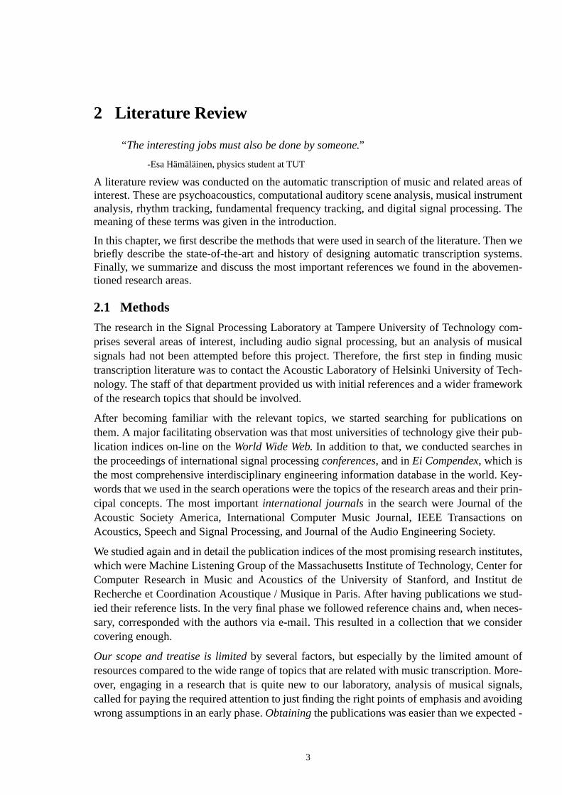
In Chapter 2, we describe a literature review on automatic music transcription and orelated areas of interest. In Chapter 3, we discuss a decomposition of the transcription printo more tractable pieces, and present some approaches that have been taken. Chapdevoted to rhythm tracking (defined in Table 1) and Chapter 5 to methods that can be utracking the fundamental frequency of sounds.The most important chapters are 6 and 7, sincthey constitute the original part of this thesis.In Chapter 6, we develop a number theoreticmethod of observing sounds in polyphonic signals. The performance of the algorithm wevaluated when we apply it to an automatic transcription of piano music in Chapter 7. Finin Chapter 8 we discuss perception-based primitive dependencies in music and so-calledown processing, which utilizes internal, high-level models and predictions in transcriptio

Table 1: Term definitions

fundamentalfrequency

Seepitch.

loudness Perceived attribute of a sound that corresponds to the physical measure soundintensity, the degree of being loud. Loudness is a psychologicaldescription of the magnitude of an auditory sensation [Moore95].

pitch Perceived attribute of sounds, which enables an ordering of sounds on ascale extending from low to high.Fundamental frequencyis a correspondingphysical (not perceptual) term. We use pitch and fundamental frequencysynonyms.

note We use the wordnotein two roles: to refer to a symbol used in musical notations and to refer to a sound that is produced by a musical instrument, wthat symbol is played.

rhythmtracking

1) Finding the times when separate sounds start and stop playing in anacoustic signal.2) Giving a description of the rhythmic structure of a muscal piece, when the timings of separate sounds have been given.A rhythm tracking system may comprise only the latter or both.

2

as ofrument. The

en wetems.emen-

com-usical

musicch-

work

onub-

in

Key-eir prin-e

on.

itutes,er fort destud-eces-sider

ofMore-gnals,idingd -

2 Literature Review

“The interesting jobs must also be done by someone.”

-Esa Hämäläinen, physics student at TUT

A literature review was conducted on the automatic transcription of music and related areinterest. These are psychoacoustics, computational auditory scene analysis, musical instanalysis, rhythm tracking, fundamental frequency tracking, and digital signal processingmeaning of these terms was given in the introduction.

In this chapter, we first describe the methods that were used in search of the literature. Thbriefly describe the state-of-the-art and history of designing automatic transcription sysFinally, we summarize and discuss the most important references we found in the abovtioned research areas.

2.1 Methods

The research in the Signal Processing Laboratory at Tampere University of Technologyprises several areas of interest, including audio signal processing, but an analysis of msignals had not been attempted before this project. Therefore, the first step in findingtranscription literature was to contact the Acoustic Laboratory of Helsinki University of Tenology. The staff of that department provided us with initial references and a wider frameof the research topics that should be involved.

After becoming familiar with the relevant topics, we started searching for publicationsthem. A major facilitating observation was that most universities of technology give their plication indices on-line on theWorld Wide Web. In addition to that, we conducted searchesthe proceedings of international signal processingconferences, and inEi Compendex, which isthe most comprehensive interdisciplinary engineering information database in the world.words that we used in the search operations were the topics of the research areas and thcipal concepts. The most importantinternational journalsin the search were Journal of thAcoustic Society America, International Computer Music Journal, IEEE TransactionsAcoustics, Speech and Signal Processing, and Journal of the Audio Engineering Society

We studied again and in detail the publication indices of the most promising research instwhich were Machine Listening Group of the Massachusetts Institute of Technology, CentComputer Research in Music and Acoustics of the University of Stanford, and InstituRecherche et Coordination Acoustique / Musique in Paris. After having publications weied their reference lists. In the very final phase we followed reference chains and, when nsary, corresponded with the authors via e-mail. This resulted in a collection that we concovering enough.

Our scope and treatise is limitedby several factors, but especially by the limited amountresources compared to the wide range of topics that are related with music transcription.over, engaging in a research that is quite new to our laboratory, analysis of musical sicalled for paying the required attention to just finding the right points of emphasis and avowrong assumptions in an early phase.Obtainingthe publications was easier than we expecte

3

sub-up-to-scrip-

ancepre-rough

ion ofcarefuld

er 1

9,90].uen-

ed

l

we failed to have only a very few publications.

2.2 Published transcription systems

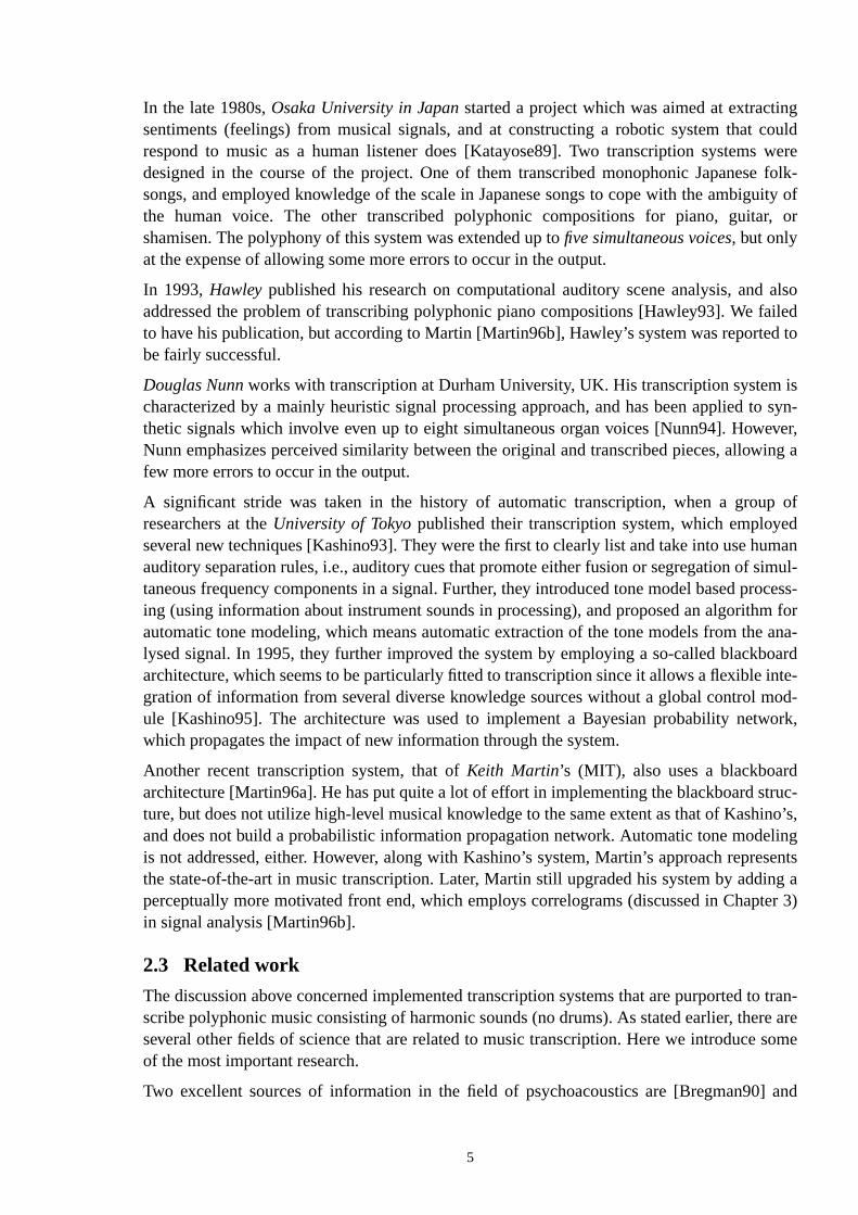
The state-of-the-art in music transcription will be discussed in coming chapters, where theproblems of the task are taken under consideration. There we will also refer to the mostdate research in different areas. In this section we will take a glance at the different trantion systems that have been presented until now.

We summarize some figures of merit of the different systems in Table 3. These performstatistics were not explicitly stated in some publications, but had to be deduced from thesented simulation material and results. For this reason, the figures should be taken ascharacterizations only. Furthermore, it is always hard to know how selective the presentatsimulation results of each system has been, and how much has been attained just by atuning of parameters. In the table,polyphonyrefers to the maximum polyphony in presentetranscription simulations,soundsrepresent the istruments that were involved,note rangegivesthe number of different note pitches involved, andknowledge usedcolumn lists the types ofknowledge that were incorporated into each system. Systemarchitectures, such as a straight-forward abstraction hierarchy or a blackboard, will be discussed in Chapter 8.

The first polyphonic transcription system, that of Moorer’s, was introduced in Chapt[Moorer75b]. Moorer’s work was carried on by agroup of researchers at Stanfordin the begin-ning of the 1980s [Chafe82,85,86]. Further development was made by Maher [Maher8However, polyphony was still restricted to two voices, and the range of fundamental freqcies for each voice was restricted to nonoverlapping ranges.

Table 2: Transcription systems

Reference Institute Performance Knowledge us

Moorer75a,b StanfordUniversity

Polyphony: 2 (severe limitations on content).Sounds: violin, guitar.Note range: 24.

Heuristicapproach.

Chafe82,85,86 StanfordUniversity

Polyphony: 2 (presented simulation resultsinsufficient).Sound: piano.Note range: 19.

Heuristicapproach.

Maher89,90 IllinoisUniversity

Polyphony: 2.Sounds: clarinet, bassoon, trum-pet, tuba, synthesized.Note ranges: severelimitation, pitch ranges must not overlap.

Heuristicapproach.

Katayose89 OsakaUniversity

Polyphony: 5 (several errors allowed).Sounds: piano, guitar, shamisen.Note r.: 32.

Heuristicapproach.

Nunn94 DurhamUniversity

Polyphony: up to 8 (several errors allowed,perceptual similarity).Sound: organ.Note range: 48.

Perceptual rules.Architecture:bottom-up abstr-action hierarchy.

Kashino93,95 TokyoUniversity

Polyphony: 3 (quite reliable).Sounds: flute, piano, trumpet,automatic adaptation to tone.Note range: 18.

Perceptual rules, timbre mod-els, tone memories, statisticachord transition dictionary.Architecture: blackboard,Bayesian probability network.

Martin96a,b MIT Polyphony: 4 (quite reliable).Sound: piano.Note range: 33.

Perceptual rules.Architecture: blackboard

4

gcould

weree folk-uity of

r, or

alsoailedd to

isto syn-ever,ing a

p ofd

umanimul-

rocess-m forana-oardinte-od-ork,

truc-ino’s,lingsents

ing ater 3)

to tran-re aresome

and

In the late 1980s,Osaka University in Japanstarted a project which was aimed at extractinsentiments (feelings) from musical signals, and at constructing a robotic system thatrespond to music as a human listener does [Katayose89]. Two transcription systemsdesigned in the course of the project. One of them transcribed monophonic Japanessongs, and employed knowledge of the scale in Japanese songs to cope with the ambigthe human voice. The other transcribed polyphonic compositions for piano, guitashamisen. The polyphony of this system was extended up tofive simultaneous voices, but onlyat the expense of allowing some more errors to occur in the output.

In 1993,Hawley published his research on computational auditory scene analysis, andaddressed the problem of transcribing polyphonic piano compositions [Hawley93]. We fto have his publication, but according to Martin [Martin96b], Hawley’s system was reportebe fairly successful.

Douglas Nunnworks with transcription at Durham University, UK. His transcription systemcharacterized by a mainly heuristic signal processing approach, and has been appliedthetic signals which involve even up to eight simultaneous organ voices [Nunn94]. HowNunn emphasizes perceived similarity between the original and transcribed pieces, allowfew more errors to occur in the output.

A significant stride was taken in the history of automatic transcription, when a grouresearchers at theUniversity of Tokyopublished their transcription system, which employeseveral new techniques [Kashino93]. They were the first to clearly list and take into use hauditory separation rules, i.e., auditory cues that promote either fusion or segregation of staneous frequency components in a signal. Further, they introduced tone model based ping (using information about instrument sounds in processing), and proposed an algorithautomatic tone modeling, which means automatic extraction of the tone models from thelysed signal. In 1995, they further improved the system by employing a so-called blackbarchitecture, which seems to be particularly fitted to transcription since it allows a flexiblegration of information from several diverse knowledge sources without a global control mule [Kashino95]. The architecture was used to implement a Bayesian probability netwwhich propagates the impact of new information through the system.

Another recent transcription system, that ofKeith Martin’s (MIT), also uses a blackboardarchitecture [Martin96a]. He has put quite a lot of effort in implementing the blackboard sture, but does not utilize high-level musical knowledge to the same extent as that of Kashand does not build a probabilistic information propagation network. Automatic tone modeis not addressed, either. However, along with Kashino’s system, Martin’s approach reprethe state-of-the-art in music transcription. Later, Martin still upgraded his system by addperceptually more motivated front end, which employs correlograms (discussed in Chapin signal analysis [Martin96b].

2.3 Related work

The discussion above concerned implemented transcription systems that are purportedscribe polyphonic music consisting of harmonic sounds (no drums). As stated earlier, theseveral other fields of science that are related to music transcription. Here we introduceof the most important research.

Two excellent sources of information in the field of psychoacoustics are [Bregman90]

5

ofmentalat are

neweres),es.auto-

f therousu-e didputa-

ction-andgree-

ainlysed inan97].cing

h con-to themma-

s for agraph-of the

fromture

thoughcking’,, theat thefrom

es onen

[Moore95].Albert Bregman’s book “Auditory Scene Analysis - the Perceptual OrganizationSound” (773 pages) comprises results of a three decade research work of this experipsychologist, and has been widely referenced in the branches of computer science threlated to auditory perception. Music perception is also addressed in the book. Another,and not so well known, is “Hearing - Handbook of Perception and Cognition” (468 pagwhich is edited byBrian Moore, and also covers research on auditory perception over timBoth of these are excellent sources of psychoacoustic information for the design of anmatic transcription system.

Computational auditory scene analysis (CASA) refers to the computational analysis oacoustic information coming from a physical environment, and the interpretation of numedistinct events in it. In 1991,David Mellingerprepared a review of psychoacoustic and neropsychological studies concerning the human auditory scene analysis [Mellinger91]. Hnot implement a complete computer model of the auditory system, but tested them comtionally, actually using musical signals as test material. More recently, the work ofDaniel Ellisrepresents the up to date research on CASA [Ellis96]. His study also comprises predidriven processing, which means utilization of the predictions of an internal world modelhigher-level knowledge. Ellis evaluated his computational model, and obtained a good ament between the events detected by the model and by human listeners.

Our research on the analysis of musical instrumental sounds was limited by time, and mcovers the sinusoidal representation, which we found the most useful. This will be discusSection 3.3. Some references on that area are [McAulay86, Smith87, Serra89,97, QiMeillier’s comment on the importance of the attack transient of a sound is worth noti[Meillier91].

Some systems have been proposed that are aimed at transcribing polyphonic music whicsists of drum-like instruments only [Stautner82, Schloss85]. Since they are more relatedsystems that track rhythm, we will discuss them in Chapter 4. Table 4 in that chapter surizes the rhythm tracking systems. Monophonic transcription, more generally calledfundamen-tal frequency tracking, will be treated in Chapter 5.

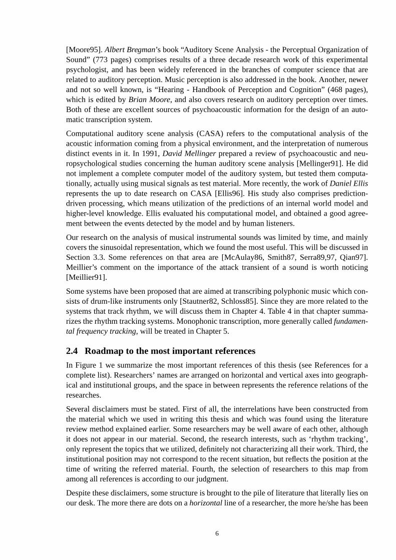
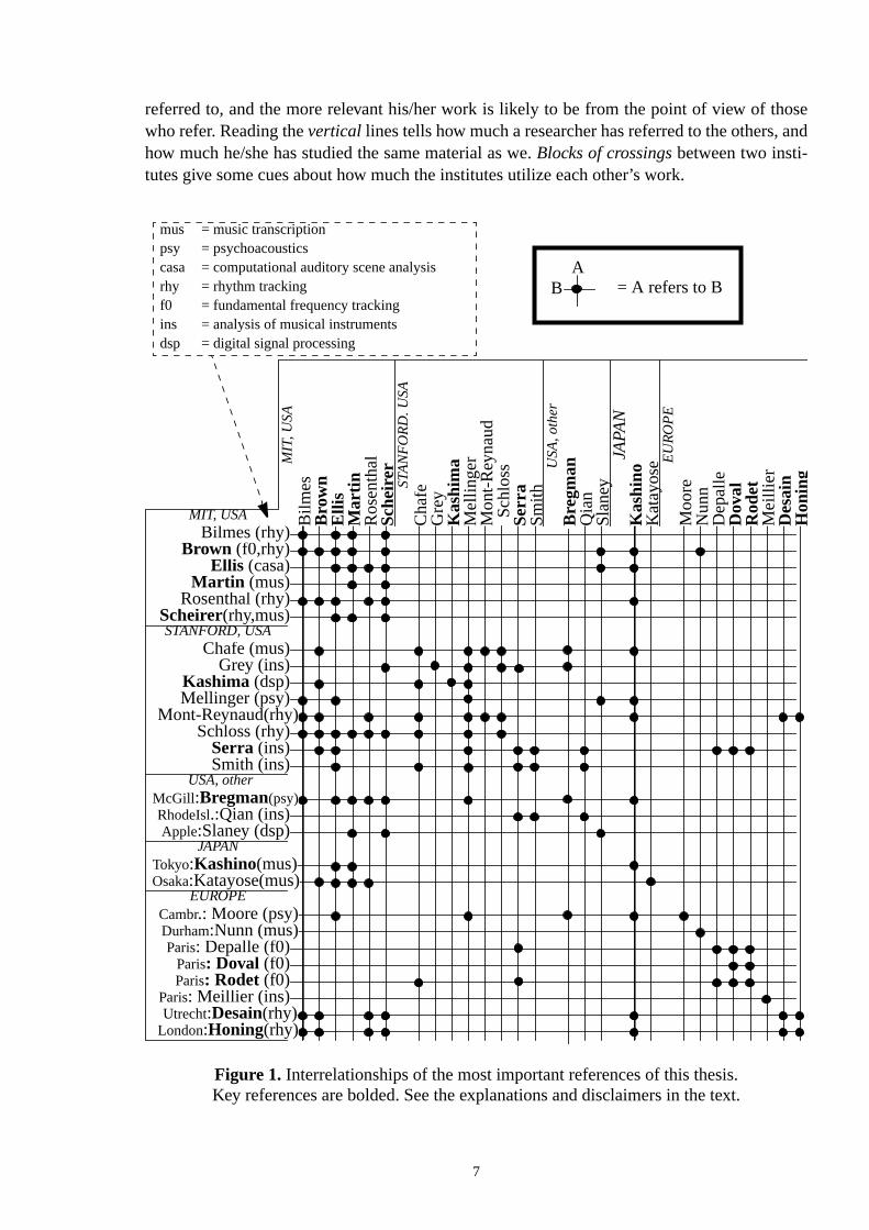
2.4 Roadmap to the most important references

In Figure 1 we summarize the most important references of this thesis (see Referencecomplete list). Researchers’ names are arranged on horizontal and vertical axes into geoical and institutional groups, and the space in between represents the reference relationsresearches.

Several disclaimers must be stated. First of all, the interrelations have been constructedthe material which we used in writing this thesis and which was found using the literareview method explained earlier. Some researchers may be well aware of each other, alit does not appear in our material. Second, the research interests, such as ‘rhythm traonly represent the topics that we utilized, definitely not characterizing all their work. Thirdinstitutional position may not correspond to the recent situation, but reflects the positiontime of writing the referred material. Fourth, the selection of researchers to this mapamong all references is according to our judgment.

Despite these disclaimers, some structure is brought to the pile of literature that literally liour desk. The more there are dots on ahorizontalline of a researcher, the more he/she has be

6

oseand

referred to, and the more relevant his/her work is likely to be from the point of view of thwho refer. Reading thevertical lines tells how much a researcher has referred to the others,how much he/she has studied the same material as we.Blocks of crossingsbetween two insti-tutes give some cues about how much the institutes utilize each other’s work.

USA, other

US

A, o

the

r

Des

ain

Qia

nS

lane

y

Mei

llier

Dov

alD

epal

le

Kas

hino

Kat

ayos

e

Nun

nM

oore

Elli

s

Sch

eire

r

Bro

wn

Bilm

es

Bre

gman

Ros

enth

al

Kas

him

a

Ser

raS

mith

Gre

y

Mel

linge

r

Sch

loss

Cha

fe

Mar

tin

Mon

t-R

eyna

ud

ST

AN

FO

RD

. U

SA

MIT

, U

SA

EU

RO

PE

JAP

AN

Hon

ing

Utrecht:Desain(rhy)

RhodeIsl.:Qian (ins)Apple:Slaney (dsp)

Paris: Meillier (ins)

Paris: Doval (f0)Paris: Depalle (f0)

Tokyo:Kashino(mus)Osaka:Katayose(mus)

Durham:Nunn (mus)Cambr.: Moore (psy)

Ellis (casa)

Scheirer(rhy,mus)

Brown (f0,rhy)Bilmes (rhy)

McGill :Bregman(psy)

Rosenthal (rhy)

Kashima (dsp)

Serra (ins)Smith (ins)

Grey (ins)

Mellinger (psy)

Schloss (rhy)

Chafe (mus)

Martin (mus)

Mont-Reynaud(rhy)

STANFORD, USA

MIT, USA

EUROPE

JAPAN

London:Honing(rhy)

Paris: Rodet (f0)

Rod

et

AB = A refers to B

mus = music transcriptionpsy = psychoacousticscasa = computational auditory scene analysisrhy = rhythm trackingf0 = fundamental frequency trackingins = analysis of musical instrumentsdsp = digital signal processing

Figure 1. Interrelationships of the most important references of this thesis.Key references are bolded. See the explanations and disclaimers in the text.

7

ble tobeen

sym-IDIand

l91].

2.5 Commercial products

Not even the first commercial transcription system has been released which would be atranscribe polyphonic music. On the contrary, monophonic transcription machines haveintegrated to several studio equipment. They include pitch-to-MIDI changers and allowbolic editing and fixing of mistuned singing, for example [Opcode96]. The achronym Mstands for Musical Instrument Digital Interface, and is a standard way of representingcommunicating musical notes and their parameters between two digital devices [Genera

8

simi-nfor-o note

of con-ump-ing at

e

refer-level

rse of

te ofrst ofstemster 8.t, will

ercep-evi-

ping.

neousisditoryration is

singleThispoly-

n.usi-

3 Decomposition of the Transcription Problem

Comparing the approaches of different transcription systems reveals a significant overalllarity in decomposing the transcription problem into more tangible pieces and in the way imation is represented at successive stages of abstraction from an acoustic signal tsymbols.

In this chapter we discuss potential approaches, abstraction hierarchies and selectionscepts in a transcription system. This is needed to reveal underlying potentially wrong asstions in our approach, and to avoid overlooking approaches that do not seem to be promisa first glance. We first discuss the relevance of thenoteas a target symbol, and then list thbasic components of a transcription system.

Most of this chapter is devoted to finding an appropriaterepresentation for information at mid-levelbetween the acoustic signal and its musical notation. The term mid-level is used toto the level of processing in auditory perception which occurs between an acoustic lowsignal reaching the ear and its cognitive high-level representation [Ellis95].

At the end of the chapter, we present a design philosophy that was formed in the coustudying these matters.

3.1 Relevance of the note as a representation symbol

Scheirer remarks on two implicit assumptions in most transcription systems: a unidirecbot-tom-upflow of information from low-level processes to high-level processes, and the usnoteas a fundamental representational symbol in music perception [Scheirer96a]. The fithese, a pure bottom-up flow of data, does not apply to the most recent transcription sy[Kashino93,95, Martin96a,b]. Top-down processing will be defined and treated in ChapThe second question, whether a note is an appropriate symbol in representation or nonow be discussed to a certain extent.

We cannot assume notes being the fundamental mental representation of all musical ption, or there being a transcription facility in brains for that [Scheirer96a]. Experimentaldence indicates that, instead of notes, humans extractauditory cuesthat are then grouped intopercepts. Predictive models that utilize musical knowledge and context are used in grou

Bregman pays attention to the fact that music often wants the listener to accept simultasounds as a single coherent sound with its own striking emergent properties. The soundchi-meric in the sense that it does not belong to any single physical source. The human ausystem has a tendency to segregate a sound mixture to the physical sources, but orchestoften called upon to oppose these tendencies and force the auditory system to create achimeric sound, which would be irreducible into perceptually smaller units [Bregman90].is a problem in music transcription, as will be seen when an attempt is made to resolvephonic musical signals in Chapter 6.

In this thesis we do not try to understand the mental processes in human music perceptioOurintention is to transcribe acoustic musical signals into a symbolic representation which m

9

mentstru-

using athat a

l usingythmicmong

s. Theing,

cess-sults, and

al toroachsuita-

gh’,he ear,ompre-sses at

usical

cians could use to reproduce the acoustic signal using a limited variety of musical instrusounds.When chimeric sounds are in question, they must be decomposed to musical inment sounds in order to be reproducible.

The symbol note expresses the fundamental frequency of a sound that should be playedcertain musical instrument. Thus, it is most appropriate and relevant as far as we requireselected symbolic representation should enable transforming it back to an acoustic signathose instruments. Additional symbols, such as the loudness of the sounds and the rhstructure of a musical composition must be added, but the symbol note is fundamental athem.

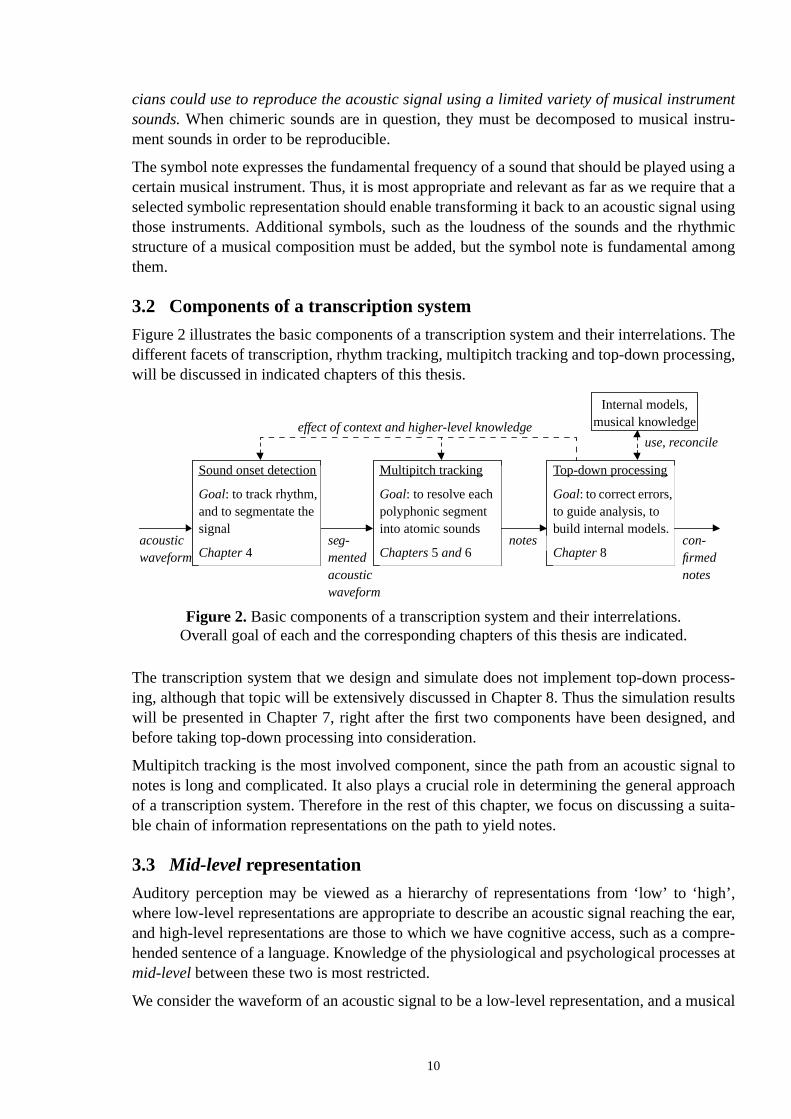
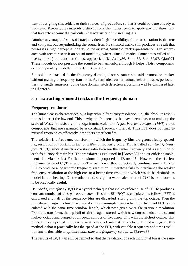
3.2 Components of a transcription system

Figure 2 illustrates the basic components of a transcription system and their interrelationdifferent facets of transcription, rhythm tracking, multipitch tracking and top-down processwill be discussed in indicated chapters of this thesis.

The transcription system that we design and simulate does not implement top-down proing, although that topic will be extensively discussed in Chapter 8. Thus the simulation rewill be presented in Chapter 7, right after the first two components have been designedbefore taking top-down processing into consideration.

Multipitch tracking is the most involved component, since the path from an acoustic signnotes is long and complicated. It also plays a crucial role in determining the general appof a transcription system. Therefore in the rest of this chapter, we focus on discussing able chain of information representations on the path to yield notes.

3.3 Mid-level representation

Auditory perception may be viewed as a hierarchy of representations from ‘low’ to ‘hiwhere low-level representations are appropriate to describe an acoustic signal reaching tand high-level representations are those to which we have cognitive access, such as a chended sentence of a language. Knowledge of the physiological and psychological procemid-level between these two is most restricted.

We consider the waveform of an acoustic signal to be a low-level representation, and a m

acousticwaveform

seg-mentedacousticwaveform

effect of context and higher-level knowledge

Sound onset detection

Goal: to track rhythm,and to segmentate thesignal

Chapter4

Multipitch tracking

Goal: to resolve eachpolyphonic segmentinto atomic sounds

Chapters 5 and 6

Top-down processing

Goal: to correct errors,to guide analysis, tobuild internal models.

Chapter 8con-firmednotes

notes

Internal models,musical knowledge

use, reconcile

Figure 2.Basic components of a transcription system and their interrelations.Overall goal of each and the corresponding chapters of this thesis are indicated.

10

ractionightlytionsr, this

cenempar-cord-

ks addi-

h actsussed.

ientlyls of,

adingrom

,

notation (notes) to be a high-level representation. Between these two, intermediate abstlevel(s) are indispensable, since the symbols of a musical notation cannot be stradeduced from the information that is present in the acoustic signal. Mid-level representaof several transcription systems were reviewed, and are listed in Table 3. As stated earliereveals a fundamental resemblance in the signal analysis of the different systems.

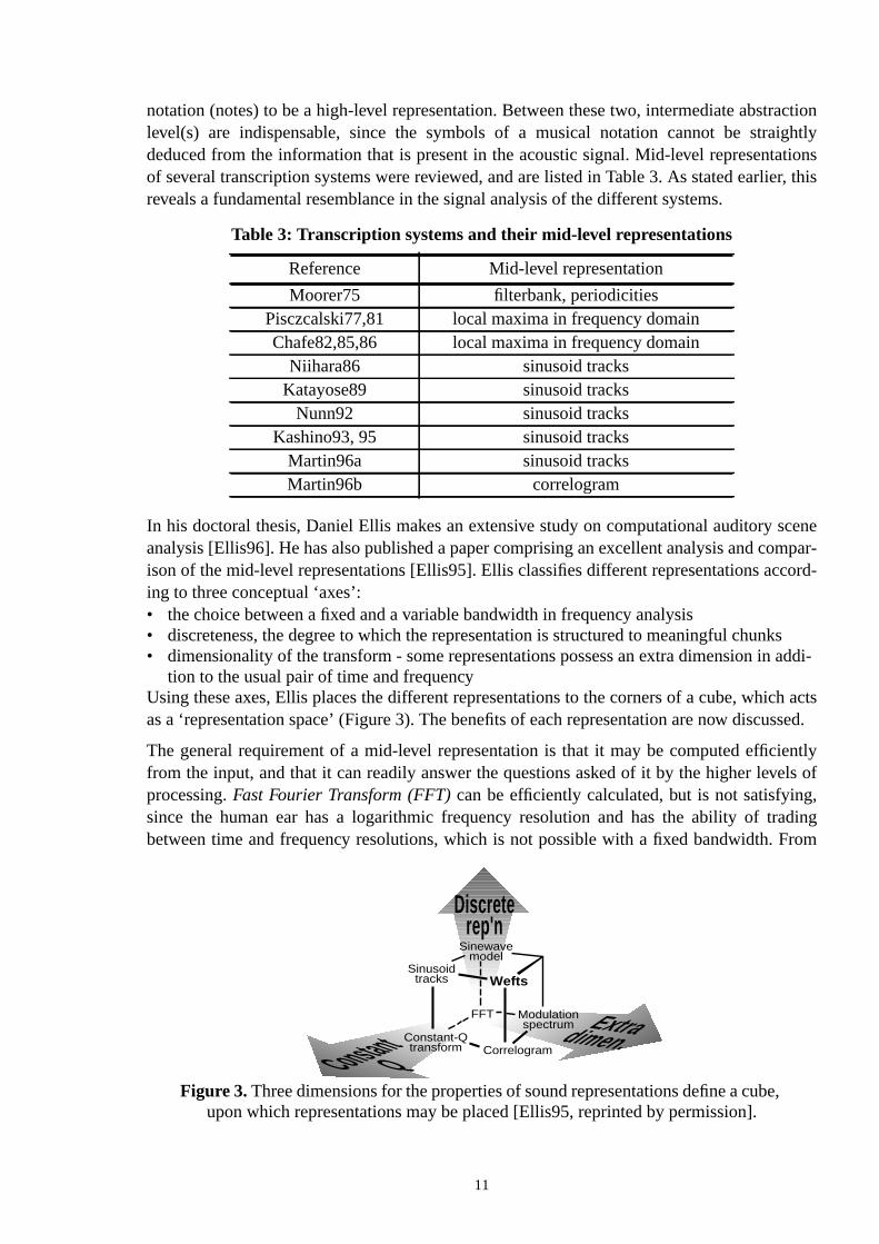
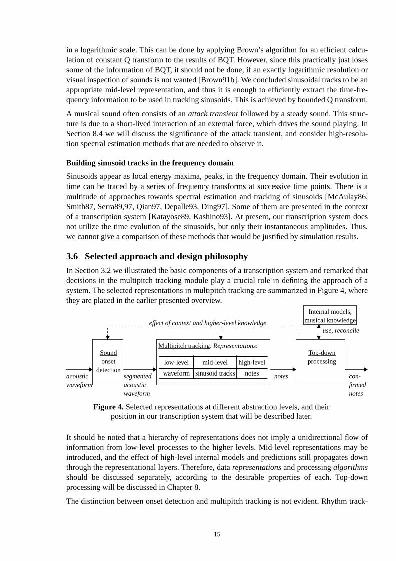
In his doctoral thesis, Daniel Ellis makes an extensive study on computational auditory sanalysis [Ellis96]. He has also published a paper comprising an excellent analysis and coison of the mid-level representations [Ellis95]. Ellis classifies different representations acing to three conceptual ‘axes’:• the choice between a fixed and a variable bandwidth in frequency analysis• discreteness, the degree to which the representation is structured to meaningful chun• dimensionality of the transform - some representations possess an extra dimension in

tion to the usual pair of time and frequencyUsing these axes, Ellis places the different representations to the corners of a cube, whicas a ‘representation space’ (Figure 3). The benefits of each representation are now disc

The general requirement of a mid-level representation is that it may be computed efficfrom the input, and that it can readily answer the questions asked of it by the higher leveprocessing.Fast Fourier Transform (FFT)can be efficiently calculated, but is not satisfyingsince the human ear has a logarithmic frequency resolution and has the ability of trbetween time and frequency resolutions, which is not possible with a fixed bandwidth. F

Table 3: Transcription systems and their mid-level representations

Reference Mid-level representation

Moorer75 filterbank, periodicitiesPisczcalski77,81 local maxima in frequency domainChafe82,85,86 local maxima in frequency domain

Niihara86 sinusoid tracksKatayose89 sinusoid tracks

Nunn92 sinusoid tracksKashino93, 95 sinusoid tracks

Martin96a sinusoid tracksMartin96b correlogram

Discreterep'n

Extradimen.ConstantQ

Wefts

Sinewavemodel

Sinusoidtracks

Constant-Qtransform

Modulationspectrum

FFT

Correlogram

Figure 3.Three dimensions for the properties of sound representations define a cubeupon which representations may be placed [Ellis95, reprinted by permission].

11

ithmi-

effi-isei- object.

uencye ats. We

ma inngtracks

pite ofsenta-g the

to as a per-

tputsin ashort-

pose

vercrite-dentf themes

theypracti-tion

tationking

rong-

tical

the music point of view, frequencies that make up the scale of Western music are logarcally spaced.

Thus we move along the ‘variable bandwidth’ axis toconstant Q transform (CQT), which pro-vides logarithmic frequency resolution. The transform is explained in [Brown88], and ancient algorithm for calculating it is given in [Brown92]. A fundamental shortcoming of FFTremoved, but CQT fails to fulfil a certain criterion given for a mid-level representation: it nther reduces the number of objects in representation nor increases the meaning of each

Both FFT and constant Q transform have been used in monophonic fundamental freqtracking [Brown91b], but it is only by moving along the two remaining axes that we arrivthe two representations that have been used in recent polyphonic transcription systemacquire a discrete representation by tracking contiguous regions of local energy maxitime-frequency, calledsinusoid tracks. This representation is particularly successful in makia discrete representation of the signal, since resynthesizing the sound from the sinusoidproduces a result that possesses a high degree of perceptual fidelity to the original, in sbeing a poor approximation in mean-squared error sense [Ellis95, Serra97]. This repretion will be further described and motivated in Section 3.4, since it is our selection amonmid-level representations.

Moving along the third axis of Ellis’s cube, to the direction of adding extra dimensionsrepresentation, is motivated by some psychoacoustic observations. Patterson proposeception model, which leads to a mid-level representation calledcorrelogram [Patterson92,Slaney93]. A correlogram is calculated by applying a short-time autocorrelation to the ouof a constant Q frequency filter bank (typically 20-40 frequency bands). This will resultthree-dimensional volume, where the dimensions are time, frequency, and lag time oftime autocorrelations applied to the outputs of filter bank filters.

Practically a correlogram means searching forperiodicitiesfrom the outputs of a filter bank.Common periodicities found at different frequency bands can be further associated to coma more discrete representation, to which Ellis gives the nameweft.Weft is a contiguous perio-dicity in time-frequency-periodicity volume, having a certain length in time and extending othe frequency bands that share the same periodicity. Weft representation fulfils anotherrion for a good mid-level representation: it tries to organize sounds to their indepensources. Actually wefts, as defined by Ellis, track periodicities in the amplitude envelope osignal, not in the signal itself. A straightforward discretization of a correlogram is someticalled a summary autocorrelogram orperiodogram.

Although quite complicated, periodograms and wefts are motivated by the fact thatexplain a wide range of psychoacoustic phenomena and oddities, and have proved to becally efficient in computational auditory scene analysis. A publicly available implementaof Patterson’s model has been released by Slaney [Slaney93].

Only one transcription system uses the correlogram as its mid-level represen[Martin96b]. A certain analogy with correlograms can also be seen in some rhythm tracalgorithms, where a bank of filters is followed by a network of resonators to detect the stest periodicities [Scheirer96b]. Rhythm tracking will be discussed in Chapter 4.

3.4 Reasons for rejecting the correlogram and choosing sinusoid tracks

We studied carefully the psychoacoustic motivations of the correlogram and its prac

12

usinginto

s wellult is

ner to”. Wepar-

ser isxture.

olvedset

r-

senta-ote isuruce anr thely aosingt canstead of

a cer-fre-icities

har-The

iew,subse-

l, notas an

ll sep-rward

appropriateness to solve concrete transcription problems. We also made simulationsSlaney’s implementation of the auditory filterbank and correlogram [Slaney93]. We camethe conclusion that the correlogram and wefts suit computational auditory scene analysiin general, but are not very appropriate to the transcription of polyphonic music. This resdefinitely not evident, and is therefore justified in the following.

The problem with the correlogram and weft analysis

Let us repeat what was said earlier about chimeric sounds: “music often wants the listeaccept simultaneous sounds as a single coherent sound with its own striking propertieswant to emphasize that this is an important principle in music in general, not only at singleticular points. A certain tendency in Western music is to pay attention to thefrequency rela-tionsof simultaneously played sounds. Two sounds are in aharmonicrelation to each other, iftheir frequencies are in rational number relations. In Section 6.3 we will show that the clothe relation, the more perfectly the notes play together and the more chimeric is their mi

Even the most typical mixtures of three notes may be so chimeric that they cannot be resusing a straightforward periodicity tracking algorithm. We pick one example from a widerthat will be given in Section 6.3: In a basic major chord, the two lower notes,C andE, overlap60 percent of the frequency partials of a third note,G. This means that sixty percent of the patials of the noteG would be found from the signal even in the absence of the noteG, and in thatcase a straightforward periodicity tracker will easily be misled to find a ‘ghost’G.

In Section 3.1 we reviewed Scheirer’s problematization of the note being a relevant repretional symbol in music perception. What was not emphasized there is that, indeed, the nnot a representational symbol for musicperception.It was accepted especially because of ointention to produce a symbolic representation that could be used by musicians to reprodacoustic signal.We suggest that human perception model as such is not appropriate fotranscription of music. An average person is not able to transcribe even the mixtures of onfew musical sounds, even if the individual sounds had been clearly introduced before pthe transcription problem. Since music transcription is not a ‘natural’ perceptual task, bube seen as separating chimeric sounds, we suggest that specific methods are needed ina general computational auditory scene analysis.

Both correlograms and weft analysis apply a short-time autocorrelation to the outputs oftain auditory filter bank. The filter bank is not intended to provide a sufficiently precisequency resolution, but it is the subsequent autocorrelation that is used for tracking periodin the signal. Utilization of autocorrelation is a problem here, sinceautocorrelation fuses infor-mation on perceptual grounds in such a way that it prevents a separate treatment of eachmonic partial that we consider necessary in order to resolve musical polyphonies.correlogram and wefts were motivated by their plausibility from a perceptional point of vbut it should be noted that these representations are so involved that they also tie thequent algorithms to themselves.

Advantages of sinusoid tracks

A weakness of sinusoid track representation is that it remains at a lower abstraction leveassigning sinusoids to their due sources of production. However, this can also be seenadvantage: the representation is very compact, but different pieces of information are stiarated from each other. This is important since in musical signals there is no straightfo

13

dy athms

cretelt thatccord-d addi-n97].

onents

trackeddici-later

esolu-up the

map to

aced,

on ofple-ient

ns ofakerle torious

e asn thecal-

tion.cond. This

of thissolu-

ame

way of assigning sinusoidals to their sources of production, so that it could be done alreamid-level. Keeping the sinusoids distinct allows the higher levels to apply specific algoritthat take into account the particular characteristics of musical signals.

Another advantage of sinusoid tracks is their high invertibility: the representation is disand compact, but resynthesizing the sound from its sinusoid tracks still produces a resupossesses a high perceptual fidelity to the original. Sinusoid track representation is in aance with recent research on sound modeling, where sinusoid models (sometimes calletive synthesis) are considered most appropriate [McAulay86, Smith87, Serra89,97, QiaThese models do not presume the sound to be harmonic, although it helps. Noisy compcan be separately modelled if needed [Serra89,97].

Sinusoids are tracked in the frequency domain, since separate sinusoids cannot bewithout making a frequency transform. As reminded earlier, autocorrelation tracks perioties, not single sinusoids. Some time domain pitch detection algorithms will be discussedin Chapter 5.

3.5 Extracting sinusoid tracks in the frequency domain

Frequency transforms

The human ear is charactericed by a logarithmic frequency resolution, i.e., the absolute rtion is better at the low end. This is why the frequencies that have been chosen to makescale of Western music are on a logarithmic scale, too. Afast Fourier transform (FFT)yieldscomponents that are separated by a constant frequency interval. Thus FFT does notmusical frequencies efficiently, despite its other benefits.

The solution is a frequency transform, in which the frequency bins are geometrically spi.e., resolution is constant in thelogarithmic frequency scale. This is calledconstant Q trans-form (CQT), since it yields a constant ratio between the center frequency and a resolutieach frequency domain bin. The transform is explained in [Brown88] and an efficient immentation via the fast Fourier transform is proposed in [Brown92]. However, the efficimplementation of CQT relies on FFT in such a way that it practically combines several biFFT to produce a logarithmic frequency resolution. It therefore fails to interchange the wefrequency resolution at the high end to a better time resolution which would be desirabmodel human hearing. On the other hand, straightforward calculation of CQT is too laboto be practically useful.

Bounded Q transform (BQT)is a hybrid technique that makes efficient use of FFT to producconstant number of binsper each octave[Kashima85]. BQT is calculated as follows. FFT icalculated and half of the frequency bins are discarded, storing only the top octave. Thetime domain signal is low pass filtered and downsampled with a factor of two, and FFT isculated with the same time window length, which now gives twice the previous resoluFrom this transform, the top half of bins is again stored, which now corresponds to the sehighest octave and comprises an equal number of frequency bins with the highest octaveprocedure is repeated until the lowest octave of interest is reached. The advantagemethod is that it practically has the speed of the FFT, with variable frequency and time retion and is thus able tooptimize both time and frequency resolution [Brown88].

The results of BQT can still be refined so that the resolution of each individual bin is the s

14

lcu-osesn orbe an-fre-form.

-g. Insolu-

tion inre is ay86,

ontextdoeshus,lts.

d thatof awhere

w ofy be

down

-down

rack-

in a logarithmic scale. This can be done by applying Brown’s algorithm for an efficient calation of constant Q transform to the results of BQT. However, since this practically just lsome of the information of BQT, it should not be done, if an exactly logarithmic resolutiovisual inspection of sounds is not wanted [Brown91b]. We concluded sinusoidal tracks toappropriate mid-level representation, and thus it is enough to efficiently extract the timequency information to be used in tracking sinusoids. This is achieved by bounded Q trans

A musical sound often consists of anattack transientfollowed by a steady sound. This structure is due to a short-lived interaction of an external force, which drives the sound playinSection 8.4 we will discuss the significance of the attack transient, and consider high-retion spectral estimation methods that are needed to observe it.

Building sinusoid tracks in the frequency domain

Sinusoids appear as local energy maxima, peaks, in the frequency domain. Their evolutime can be traced by a series of frequency transforms at successive time points. Themultitude of approaches towards spectral estimation and tracking of sinusoids [McAulaSmith87, Serra89,97, Qian97, Depalle93, Ding97]. Some of them are presented in the cof a transcription system [Katayose89, Kashino93]. At present, our transcription systemnot utilize the time evolution of the sinusoids, but only their instantaneous amplitudes. Twe cannot give a comparison of these methods that would be justified by simulation resu

3.6 Selected approach and design philosophy

In Section 3.2 we illustrated the basic components of a transcription system and remarkedecisions in the multipitch tracking module play a crucial role in defining the approachsystem. The selected representations in multipitch tracking are summarized in Figure 4,they are placed in the earlier presented overview.

It should be noted that a hierarchy of representations does not imply a unidirectional floinformation from low-level processes to the higher levels. Mid-level representations maintroduced, and the effect of high-level internal models and predictions still propagatesthrough the representational layers. Therefore, datarepresentationsand processingalgorithmsshould be discussed separately, according to the desirable properties of each. Topprocessing will be discussed in Chapter 8.

The distinction between onset detection and multipitch tracking is not evident. Rhythm t

Multipitch tracking.Representations:

low-level mid-level high-level

waveform sinusoid tracks notesacousticwaveform

segmentedacousticwaveform

effect of context and higher-level knowledge

Soundonset

detection

Top-downprocessing

con-firmednotes

notes

Internal models,musical knowledge

use, reconcile

Figure 4.Selected representations at different abstraction levels, and theirposition in our transcription system that will be described later.

15

s are

been

r-

gicalrip-m of

ools to

llentt suit-ely anddenciesfound

more

ing might also take place together with the sinusoid tracking, in which case the onset timededuced from the onsets of the sinusoids. Figures 2 and 4 just depict our approach.

A certain design philosophy was formed in the course of studying the literature that hasshortly reviewed. It is: at each abstraction level we must first knowwhatinformation is needed,then decidehow to extract it, and finallyanalysethe reliability and dependencies of the obsevations. This philosophy is reflected in the selections and motivations presented above.

The order of questions “what” and “how” means that we use psychoacoustic and physioloknowlegde primarily for knowing what information should be observed in a music transction system, not for knowing how to extract the information. In other words, the mechanisthe human ear must not determine the information of interest. Instead, we studyauditory cuesof a human listener in segregation and fusion of musical sounds, and seach for analysis textract that information.

How to know the relevant psychoacoustic information in music perception? Two excesources in the field of psychoacoustics are [Bregman90] and [Moore95]. What is the mosable analysis method? The one that extracts the desired pieces of information as separatprecisely as possible. How to analyze the observations we obtain? Properties and depenof musical signals will be discussed at length in Chapter 6, other sources of error may bein the analysis methods chosen.

In coming chapters, the different components of a transcription system are discussed indetail.

16

on-truly

f con-roduces93].auto-

of they anoly-easierhave

poly-

ats,the

top athyth-

re sep-, andonseted as a

in aof the

d inonstra-ignalhmick is

4 Sound Onset Detection and Rhythm Tracking

“There is no doubt that music devoid of both harmony and melody can still contain csiderable expression. Percussive music is a case in point, as anyone who hasenjoyed traditional music from Africa, India, or Central or South America knows.”

-Jeffrey Bilmes [Bilmes93]

Expressive decisions in even performing a certain sequence of drum hits can carry a lot otent and meaning. This fact motivates the design of models that computers can use to pexpressivesounding rhythmic phrases instead of artificial quantized sequences [BilmeFurther, interpreting the rhythmic role of each sound or finding the downbeat and upbeatmatically from a musical signal is anything but trivial.

But let us grossly drop out both understanding the expressive meaning and interpretationrhythmic role of each sound, trying first just to detect the onset times of the sounds. Bonset timewe mean the time instant when a sound starts playing. As transcription of pphonic music is concerned, we consider the detection of the onsets of the sounds by farthan a subsequent analysis of each rhythmic segment. And truly: commercial devicesbeen released that synchronize to musical rhythm, but not even the first transcriber ofphonic music.

Rhythmic meteris a framework in which musical events are located in time. It comprises behierarchies and grouping. We did not have the possibility to study rhythm tracking withsame thoroughness and attempt as polyphonic transcription. This is why we practically sthe level of sound onset detection and do not make a further analysis of the underlying rmic structure. Our original contribution to onset detection will also be quite limited.

4.1 Psychoacoustic bounds

A human ear is able to distinguish successive onsets of sounds from each other if they aarated by at least a 20 ms time interval, varying somewhat from an individual to anotherdepending on the loudness of the sounds. If the interval is shorter, the former or loudermasksthe other one, and if there is a series of such successive onsets, they are perceivsingle rolling, low frequency sound. However, humans can detect even down to 5 mstime devi-ations in a rhythmic repetition of equidistant events [Bilmes93, Scheirer95].

We use the wordprominenceto refer to the strength at which an onset event stands outmusical signal. The prominence of an onset is a result of several attributes: frequencyattacking sound, its relative change in the amplitude, and the rapidity of the change.

4.2 Onset time detection scheme

A system capable of extracting rhythmic meter from musical signals is presente[Scheirer96b]. On a corresponding web page, Scheirer provides a psychoacoustic demtion on beat perception. The given set of audio signals shows that certain kinds of smanipulations and simplifications can be performed without affecting the perceived rhytcontent of a musical signal. The demonstration is roughly as follows. First, a filter ban

17

elopends ofkindsameeter

d that’. Theercus-fof a

of thextract

f sim-tuden ledort ofrmed

end

s mostat wasw-passally

usedThe fil-hest a2 and

n dec-con-

rmst recent

ke our

onsetood

he

designed which divides a musical signal into six frequency bands, and the amplitude envof the signal at each frequency band is calculated. Then the corresponding frequency baa noise signal are controlled by the amplitude envelopes of the musical signal. For manyof filter banks, the resulting noise signal has a rhythmic percept which is significantly the sas that of the original music signal. Even with just four frequency bands, the pulse and mcharacteristics of the original signal are easily recognizable. It should be emphasizeScheirer’s system is predominantly concerned with musical signals having a ‘strong beatabove simplifications cannot be made for, e.g., classical music, which consists of non-psive sounds only, such as a violin or an organ. Apercussive soundis defined to be the sound oa musical instrument in which the sound is set on by striking, or by a short-lived contactdriving force.

Since the only thing preserved in the above transformation is the amplitude envelopesfilter bank outputs, it seems reasonable that only that much information is necessary to epulse and meter from a musical signal [Scheirer96b]. On the other hand, certain kinds oplifications arenot possible. For example, using only one frequency band, i.e., the amplienvelope of the signal as a whole, will confuse the rhythmic percept. This observatioScheirer to make a psychoacoustic hypothesis regarding rhythm perception: some scross-band rhytmic integration, not simply summation across frequency bands, is perfoby the auditory system. Based on the above considerations, Scheirer concludes that arhythmicprocessing algorithm should treat frequency bands separately, combining results in the,rather than attempting to perform beat-tracking on the sum of filter bank outputs.

We take this result as a foundation to our onset detection system, which therefore bearresemblance to that of Scheirer. A couple of years earlier Bilmes proposed a system thon a way to the same direction, but his system only used two bands, a high-pass and a lofilter, which was not as effective [Bilmes93]. Older rhythm tracking systems have typicused the amplitude envelope of a signal as a whole [Chafe85].

Distinct frequency bands and extracting their amplitude envelopes

As motivated above, the input signal is first divided into distinct frequency bands. Weseven one-octave bands and basically the same filter bank implementation as Scheirer.ters are sixth order band-pass elliptic filters, the lowest being a low-pass filter and the highigh-pass filter. Frequency band boundaries were set to 127, 254, 508, 1016, 2034064 Hz.

The output of each band is rectified (i.e., the absolute value of the signal is taken) and theimated to ease the following computations. Amplitude envelopes are then calculated byvolving the signals with a 50 ms half-Hanning (raised cosine) window. This window perfomuch the same energy integration as the human auditory system, emphasizing the mosinputs but masking rapid modulation [Scheirer96b, Todd92].

Calculating bandwise onset times

Until now, our system has been essentially analogous to Scheirer’s one, but here we taown direction. Both Scheirer and Bilmes calculate afirst order difference functionof theamplitude envelopes, taking the maximum rising slope of the amplitude envelope as thetime of a sound [Bilmes93]. For us, it seems that a first order difference function is a gmeasure for theprominenceof the onset, but its maximum values fail to precisely mark t

18

e toiallyen notr dif-

latinge firstThenfirstnal

rele-mountffec-earlierack ofs, weure 5.

eak

maxi-e.

onsets arewhich

ndoweshold

onsettimes. This is due to two reasons. First, especially low sounds may take some timcome to the point where their amplitude is maximally rising, and thus that point is cruclate from the physical onset of a sound. Second, the onset track of a sound is most oftmonotonically increasing, and thus we would have several local maxima in the first ordeference function near the physical onset (see plots with a dashed line in Figure 5).

We took an approach that effectively handles both of these problems. We begin by calcua first order difference function, and take into account only the signal segments where thorder difference, i.e., the prominence of incoming activity, is above a certain threshold.we divide the first order difference function by the amplitude envelope function to get aorderrelative difference function, i.e., the amount of change in relation to the absolute siglevel. This is the same as differentiating the logarithm of the amplitude envelope.

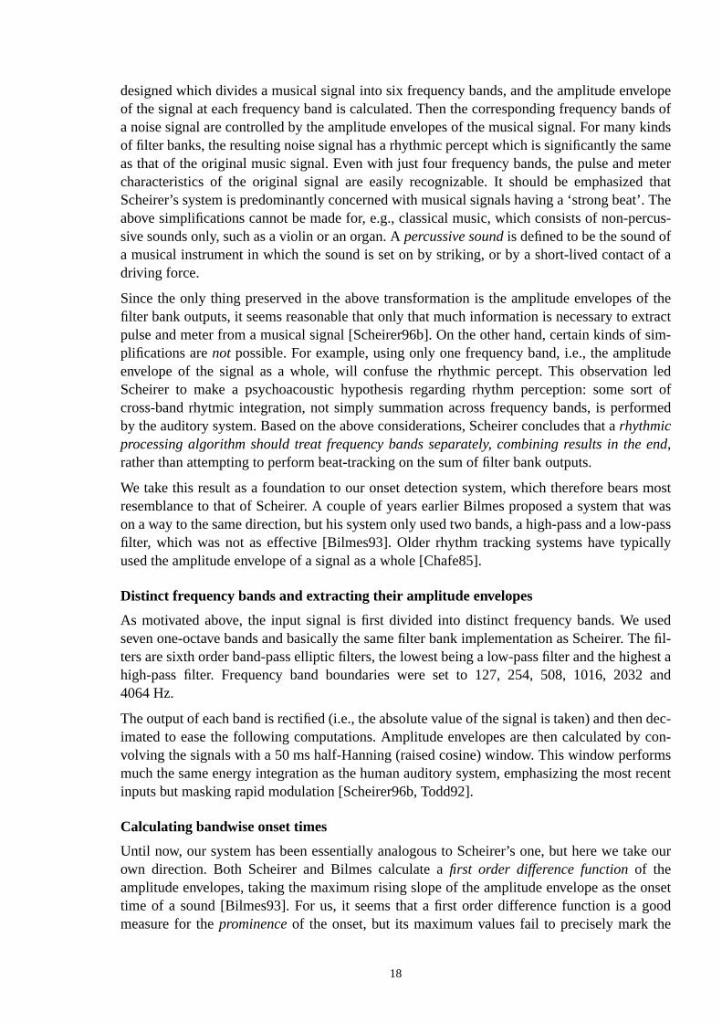
We use the relative difference function to track onset times. This is psychoacousticallyvant, since the perceived increase in signal amplitude is in relation to its level, the same aof increase being more prominent in a quiet signal. Moreover, the relative difference etively handles the abovementioned problems by detecting the onset times of low soundsand, more important, handling complicated onset tracks, since oscillations in the onset tra sound do not matter in relative terms after its amplitude has started rising. To clarify thiplotted the absolute and relative difference functions of the onset of a piano sound in FigBoth of the benefits discussed can be seen clearly.

A set of potential onsettimesare collected from each band by performing a thresholded ppicking operation to the relative difference signals. The correspondingprominencesof thepotential onsets are found by taking the time of an onset, scanning forward to the nextmum in theabsolute difference function, and taking the maximum value as the prominenc

Combining the results from different frequency bands

In the final phase we combine the results from different frequency bands to yield thetimes and prominences of the overall signal. First the potential onsets from different bandall sorted in time order. Then each onset candidate is assigned a new prominence value,is calculated by summing the prominences of onset candidates within a 50 ms time wiaround them. We drop out onset candidates whose prominence falls below a certain thr

0.8 0.9 1 1.1 1.2 1.3 1.4

x 104

10

20

30

40

50

60

frequency band

6

5

4

3

2

1

Dashed line:

Solid line:

where denotes theamplitude envelope function.

ddx------ f x( )( )

ddx------ f x( )( )log( )

f x( )

Figure 5.First orderabsolute(dashed) andrelative(solid) difference functions of theamplitude envelopes of different frequency bands. Picked onset times are circled.

19

t can-hosen

ets inratelyusic asmen-ll pre-esholds.

ciency.storedp waserpts

ts andction

value. Then we also drop out candidates that are too close (< 50 ms) to a more prominendidate. Among equally prominent but too close candidates, the middle one (median) is cand others are abandoned. Remaining onsets are accepted as true ones.

4.3 Procedure validation

The presented procedure was validated by testing its performance in finding sound onspolyphonic piano recordings and in rhythm music. Polyphonic piano recordings are sepataken into consideration, because our transcription system (see Chapter 7) uses piano msimulation material, and will utilize the presented onset detection procedure for signal segtation. The onset detection procedure was not tailored for each simulation case, but asented results have been computed using the very same set of parameter values and thr

Polyphonic piano recordings

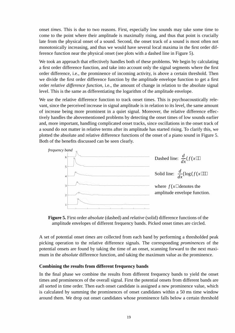
Chosen piano compositions were played and recorded to evaluate onset detection effiWe used two microphones to pick the sound of an acoustic upright piano (Yamaha) andthe signals on a digital audio tape using a 48kHz sampling rate. The microphone setuaccording to a typical studio convention [Pawera81]. Note onsets were tracked in two excof ten seconds, and the results are presented in Figure 6.

A recording comprising several instruments

Onset detection results are given for an example recording comprising several instrumendrums [Grusin91]. We consider one example sufficient, since reviewing the onset dete

0 0.5 1 1.5 2 2.5 3 3.5 4 4.5

x 104

−1.5

−1

−0.5

0

0.5

1

1.5Beethoven: "Fur Elise", part II

0 0.5 1 1.5 2 2.5 3 3.5 4 4.5

x 104

−1

−0.5

0

0.5

1

1.5Bach: "Inventio 8" for two voices

Figure 6.Tracked onsets in two piano compositions. Erroneous extra onsetsare marked with arrows, missing onsets were added and are circled.

samples

samples

20

ure 7.of thetmicallowextra

tomati-eansginachctive

struc-sym-

proc-MIDIr and

use totizedmetricmes’s

nd itsAlsoafe85].msludeswith

ro-led.

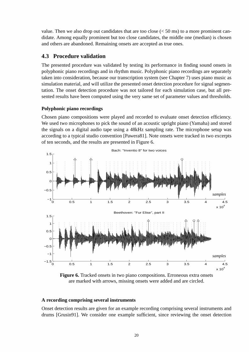
results is a laborious task without the notes of the piece. The results are presented in FigThis test case was successful, too. However, we noticed that more reliable detectiononsets in musical signals that comprise different kinds of musical styles would call for rhymeter generation and rhythm analysis after onset detection (see Section 4.4). This wouldusing prediction rules to recognise the weakest onsets and still not inserting erroneousonsets.

4.4 Rhythmic structure

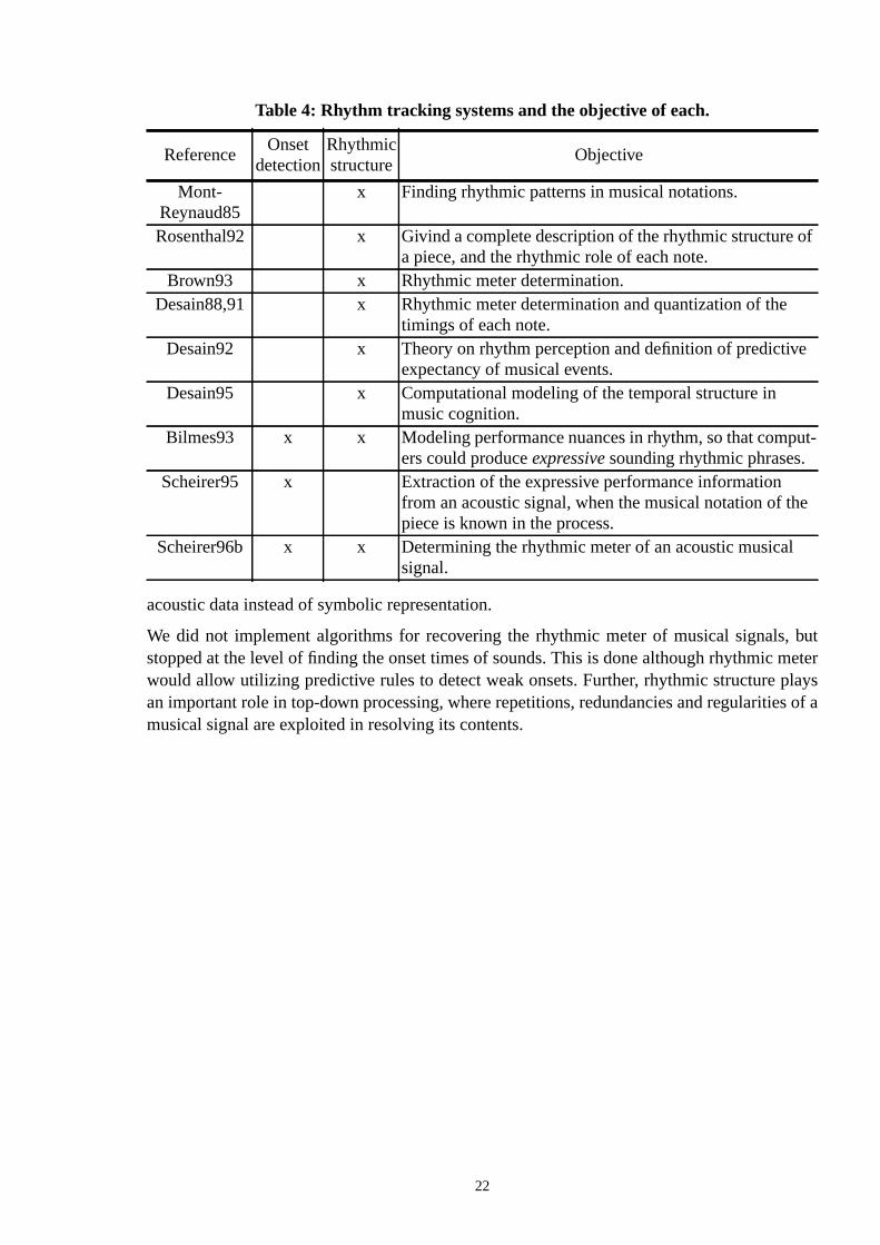
Several attempts have been made to understand the human rhythm perception and to aucally determine the rhythmic meter of a musical signal. Determining rhythmic meter mclassifying the structure of a musical piece tokey signatures, such as 3/4 or 4/4, and parsinmusical events into units calledmeasuresthat are separated from each other by vertical linesmusical notation [Brown93]. Still one step further is to understand the rhythmic role of enote. We summarize the different rhythm tracking proposals in Table 4, describe the objeof each, and indicate if they comprise onset detection in an acoustic signal or rhythmicture determination, or both. Those that do not implement the former take their input in abolic form, for example in MIDI streams.

In his doctoral thesis, David Rosenthal describes a computer program which models theesses by which humans perceive rhythm in music [Rosenthal92]. His program reads astream and gives a complete description of the rhythmic structure of the piece, its metethe rhythmic role played by each note.

Jeffrey Bilmes aimed at designing algorithms and learning strategies that computers canproduce expressive sounding rhythmic phrases, instead of artificial, exactly quansequences. He describes four elements with which he characterizes musical rhythm:structure, tempo variation, deviations, and ametric phrases. For a closer review on Bilstudies, see [Bilmes93].

Peter Desain and Henkjan Honing have published a lot about human rhythm perception acomputational modeling. To review their work see, for example, [Desain88,91,92,95].several other approaches have been taken, the earliest being e.g. [Moorer75b] and [ChBrown employed autocorrelation to determine the rhythmic meter in MIDI-strea[Brown93]. The abovementioned system of Scheirer’s is unusual in the sense that it increal-time acoustic pattern recognition, which allows the subsequent models to work

0 0.5 1 1.5 2 2.5 3

x 104

−1

−0.5

0

0.5

1

1.5Dave Grusin: "Punta del Soul"

samples (x 104)

Figure 7.Tracked onsets in a recording comprising several instruments and drums. Erneous extra onsets are marked with arrows, missing onsets were added and are circ

21

butmeterlayss of a

of

e

ut-

e

l

acoustic data instead of symbolic representation.

We did not implement algorithms for recovering the rhythmic meter of musical signals,stopped at the level of finding the onset times of sounds. This is done although rhythmicwould allow utilizing predictive rules to detect weak onsets. Further, rhythmic structure pan important role in top-down processing, where repetitions, redundancies and regularitiemusical signal are exploited in resolving its contents.

Table 4: Rhythm tracking systems and the objective of each.

ReferenceOnset

detectionRhythmicstructure

Objective

Mont-Reynaud85

x Finding rhythmic patterns in musical notations.

Rosenthal92 x Givind a complete description of the rhythmic structurea piece, and the rhythmic role of each note.

Brown93 x Rhythmic meter determination.Desain88,91 x Rhythmic meter determination and quantization of the

timings of each note.Desain92 x Theory on rhythm perception and definition of predictiv

expectancy of musical events.Desain95 x Computational modeling of the temporal structure in

music cognition.Bilmes93 x x Modeling performance nuances in rhythm, so that comp

ers could produceexpressive sounding rhythmic phrases.Scheirer95 x Extraction of the expressive performance information

from an acoustic signal, when the musical notation of thpiece is known in the process.

Scheirer96b x x Determining the rhythmic meter of an acoustic musicasignal.

22

phase,tran-

igh.unda-l nota-

n anoduc-hmicentialpara-t al.

ic sig-ana-

uency

l

gh

unda-

s,

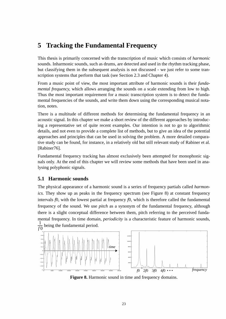
5 Tracking the Fundamental Frequency

This thesis is primarily concerned with the transcription of music which consists ofharmonicsounds. Inharmonic sounds, such as drums, are detected and used in the rhythm trackingbut classifying them in the subsequent analysis is not discussed - we just refer to somescription systems that perform that task (see Section 2.3 and Chapter 4).

From a music point of view, the most important attribute of harmonic sounds is theirfunda-mental frequency, which allows arranging the sounds on a scale extending from low to hThus the most important requirement for a music transcription system is to detect the fmental frequencies of the sounds, and write them down using the corresponding musication, notes.

There is a multitude of different methods for determining the fundamental frequency iacoustic signal. In this chapter we make a short review of the different approaches by intring a representative set of quite recent examples. Our intention is not to go to algoritdetails, and not even to provide a complete list of methods, but to give an idea of the potapproaches and principles that can be used in solving the problem. A more detailed comtive study can be found, for instance, in a relatively old but still relevant study of Rabiner e[Rabiner76].

Fundamental frequency tracking has almost exclusively been attempted for monophonnals only. At the end of this chapter we will review some methods that have been used inlysing polyphonic signals.

5.1 Harmonic sounds

The physical appearance of a harmonic sound is a series of frequency partials calledharmon-

ics. They show up as peaks in the frequency spectrum (see Figure 8) at constant freq

intervalsf0, with the lowest partial at frequencyf0, which is therefore called the fundamenta

frequency of the sound. We usepitch as a synonym of the fundamental frequency, althou

there is a slight conceptual difference between them, pitch referring to the perceived f

mental frequency. In time domain,periodicity is a characteristic feature of harmonic sound

being the fundamental period.1f 0------

0 50 100 150 200 250

200

400

600

800

1000

1200

frequency0 500 1000 1500 2000 2500 3000 3500 4000 4500−1

−0.8

−0.6

−0.4

−0.2

0

0.2

0.4

0.6

0.8

1

Figure 8.Harmonic sound in time and frequency domains.

time

f0 2f0 3f0 4f0 • • •

23

.ing ahar-

ig-

take astru-tionaln in

unda-cor-lationantd fre-

dition,largeibutese more

-cross-

f thetruell asvalue

A harmonic sound can be modelled as a sum of sinusoid partials

(1)

whereaj(t) are the amplitudes,fj(t) the frequencies, andϕj phases of the partials. For strictlyharmonic sounds, frequenciesfj(t) are , wheref0(t) is the fundamental frequencyHowever, even the sounds of musical instruments may deviate a little from this rule durshort attack transient of the sound (approximately 50 ms in length), thus not being strictlymonic.

5.2 Time domain methods

Autocorrelation-based

The autocorrelation function is particularly useful in identifying hidden periodicities in a snal. An estimate of the autocorrelation of anN-length sequencex(k) is given by

(2)

wheren is alag, or period length, andx(n) is a time domain signal.

Many autocorrelation-based fundamental frequency trackers have been proposed. Wequite recent example. In 1990, Brown published results of a study where the pitch of inmental sounds was determined using autocorrelation [Brown91a]. She tried both convenand ‘narrowed’ autocorrelation, which basically provides a better periodicity resolutioexchange to a weaker time resolution [Brown89].

The purpose of the study was to determine whether autocorrelation is well-adapted to fmental frequency tracking of musical signals, and under which conditions ‘narrowed’ autorelation is advantageous. We skip the details concerning the calculation of the autocorrefunction and the selection of a winning periodicity in it [Brown91a]. What is most importhere is that Brown suggests both conventional and narrowed autocorrelation to be gooquency trackers for musical sounds. However, autocorrelation is not very suitable forpoly-phonicmusical signals because of the reasons that were discussed in Section 3.4. In adboth Doval et al. and Rabiner remark that autocorrelation is not very suitable, when arange of pitches and variety of spectra is encountered [Doval91, Rabiner76]. These attrapply especially to music. For these reasons, we consider autocorrelation methods to badequate to speech than to musical signals.

Waveform-based

Some pitch detectors are based on time domain peak and valley measurements, or zeroing measurements. For example, Miller’s algorithm first detectsexcursion cyclesin the wave-form by observing intervals between major zero crossings [Miller75]. The remainder oalgorithm tries to identify the principal excursion cycles, i.e., those which correspond topitch periods. The algorithm was reported to work moderately well, although not as wesome other methods [Rabiner76]. Nowadays, the approach is practically of a historicalonly.

s t( ) aj t( ) f j t( ) 2πt⋅ ϕ j+[ ]cos⋅j 1=

N

∑=

j f 0 t( )⋅

r xx n( ) 1N---- x k( ) x k n+( )⋅

k 0=

N n– 1–

∑⋅=

24

ries of

ics

prob-lowl-quiten to aheytationandand

ioned

con-ctionlogictions,loyed.

abil-ts forplyinges an

nd theis isut uti-ctrumm),auto-

itchFou-nallye sig-

ge of

5.3 Frequency domain methods

Harmonic matching pitch detection

As stated earlier, the appearance of a harmonic sound in the frequency domain is a seequidistant energy maxima, at the positions of the harmonic partials.Harmonic matching fre-quency domain pitch detectionmeans looking for a fundamental frequency, whose harmonbest explain the partials in a signal [Hess83].

A method proposed by Doval and Rodet belongs to this class [Doval91]. It is based on aabilistic model for calculating the likelihood of anf0, when the frequency partials in a signaare known. The method is flexible enough to take into account possibly available prior knedge of the sound in question. A mathematical expression for calculating the likelihood iscomplicated and can be found in the reference. The researchers paid particular attentiolarge range of applicablef0s (50-4000 Hz), and to a very short response delay (20 ms). Ttested the algorithm with musical and speech signals and proposed a real time implemenof it. We made rather extensive simulations with Doval’s algorithm, and it proved flexibleworked well. The method employs a separate probabilistic treatment for the frequenciesamplitudes of each harmonic partial in the signal. This is important when the abovementobjectives, large range off0s and flexibility, are aimed at.

Doval and Rodet later published a higher level structure, which can be used for imposingstraints on the evolution of the signal, and for removing single gross errors in pitch deteby tracking the pitch contour through successive time frames [Doval93]. The higher levelwas based on hidden Markov models and the Viterbi algorithm. In the presented simulathe gross error rate still decreased significantly when the higher level structure was emp

Other frequency domain methods

There is a variety of methods that are more straightforward, or ‘brute force’, than the probistic approach of Doval et al. The structure of the spectrum of a harmonic sound promprevealing the fundamental frequency, the interval between the equidistant maxima, by apautocorrelation to the magnitude of the spectrum. We take two examples. Lahat describalgorithm, where the spectrum of the signal is flattened by a bank of bandpass filters, apitch is extracted from autocorrelation functions at the output of the filters [Lahat87]. Thsomewhat more sophisticated than the straightforward autocorrelation of the spectrum, blizes the very same principle. Also Kunieda uses the autocorrelation function of the speof a signal [Kunieda96]. Their method is called ACLOS (AutoCorrelation of LOg Spectrusince they take the logarithm of a magnitude spectrum, flatten the result, and calculate itscorrelation function to provide information of the pitch.

A cepstral pitch detectionmethod has also been widely used, especially in extracting the pof speech signals [Noll64, Rabiner76]. A cepstral is calculated by first taking a short timerier transform of a signal segment, then calculating the logarithm of its magnitude, and fiinverse Fourier transforming the result. The peak cepstral value determines the pitch of thnal. The problem with cepstral pitch detection is that it cannot handle a very large ranpitches, which would be desirable in processing musical signals.

25

intothodstribu-

trans-at dif-tant Q

posi-l fre-d onthe

g the-

tions.e needped a

sed todis-usicalters ofa net-

ed inpeechectionlarlyCom-

hen the

iate ascon-makely arisewith

more

low a

5.4 Utilizing prior knowledge of the sound

The earlier mentioned pitch detection method of Doval et al. is flexible enough to takeaccount prior knowledge of the sound in question [Doval91]. There are several other methat rely even more heavily on prior knowledge of the sound source and the spectral distion of the sounds. In the following, we take two examples.

In [Brown91b], Brown proposes a method that utilizes the fact that a constant Q spectralform (see Section 3.5) gives a constant frequency domain pattern for harmonic soundsferent pitches. Thus she calculates the cross-correlation function between the consspectrum and the ideal pattern of the sound in question, or just the pattern of one’s at thetions of the harmonics. A peak in the cross-correlation function reveals the fundamentaquency. We thoroughly simulated the method in a transcription system that is reviewepage 65. It proved to work fairly well for monophonic signals. Brown emphasizes thatmethod is able to deal with a variety of sounds and is consistent with the pattern matchinory of human pitch perception [Gerson78].

Spectra of musical sounds vary a lot and comprise ambiguous spectral energy distribuThe success of many proposed methods to cope with such sounds is often qualified by thto carefully tailor parameters to yield desired results. Taylor and Greenhough have develosystem which uses an adaptive resonance theoryneural networkcalled ARTMAP [Taylor93,Grossberg76]. In a preliminary phase, the network istrained by pitches from several instru-ments to achieve a tolerance to spectral variations. After training, the network can be uclassifynew signals to their due pitches. Input to the network comes from logarithmicallyributed frequency bins (12 per octave), output is a quantized pitch classification on a mscale. The general idea of neural networks seems promising especially in tuning paramea system, but they do not remove the need for algorithm design, since the topology ofwork sets limits to the model it can represent [Pao89].

5.5 Detection of multiple pitches

Determining the fundamental frequency of musical sounds has been relatively little explorcomparison to the massive efforts in estimating the pitch of speech signals for use in sencoders and for communication purposes [Brown91a]. This is also the reason why detof multiple pitches has been almost a neglected problem. Multipitch detection is particuneeded in the analysis of musical signals and in computational auditory scene analysis.mercial interest of these areas is not as high as that of speech processing, especially wdifficulty of the problem is taken into account.

The need for a multipitch detector

It is generally admitted that the pitch detection methods discussed above are not approprsuch to the detection of multiple pitches. This is especially true when musical signals arecerned, since very often the frequency relations of simultaneous sounds in music eitherseveral sounds appear as a single coherent sound, or a non-existent ‘ghost’ sound strongjust because of the joint effect of the others. We reviewed this phenomenon in simulationsseveral pitch detection algorithms. Its cause was mentioned in Section 3.4, and will beextensively discussed in Sections 6.2 and 6.3.

The problem cannot be solved by designing a sophisticated peak picking algorithm to fol

26

pitchns oftion of

ss of itforcelance, untilhocastssed.

h fromlved,

t.

ucedbased

sys-ard tohad aonly

ntainsg then in as fol-

stem.s. Theustic

96a].undslittleare inltipleoundseptual

single pitch detector. Consider, as an example, two sounds that are an octave apart infrom each other: the harmonic partials of the higher sound match perfectly the positioeven partials of the lower one, making it appear as a single sound, and turning the separathe sounds into an even theoretically ambiguous problem.

In this section we represent methods that have been used to solve the problem. Awarenedates back to the very beginning of music transcription. In 1985, Chafe remarked: “Brutedetection schemes are less likely to succeed in analyzing polyphonic input - - - The babetween underdetection and overdetection becomes more difficult to achieve”. Howeververy recently the problems of multipitch tracking have been controlled by heuristic adtechniques, borrowing algorithmic principles from single pitch tracking. It is only in the pfew years that seriously motivated methods have been proposed. They will now be discu

Tone model based processing

The abovementioned example of separating two sounds that are an octave apart in pitceach other is theoretically ambiguous without prior knowledge of the sounds. It can be sohowever, if such information is collected totone models, and utilized in signal analysis. Tonemodels are data structures that represent the spectral features of sounds in some forma

Two pitch tracking approaches that utilize knowledge of the involved sounds were introdin Section 5.4. Kashino and Tanaka were the first to describe a complete tone modelmusic transcription system [Kashino93]. They also proposed an algorithm forautomatic tonemodeling, which means extraction of the tone models from the analyzed signal itself. Thetem suffered from some severe limitations, but was, on the contrary, more generic in regthe types of instrumental sounds. In simulations, an advance registration of tone modelssignificant effect on transcribing three-voice polyphonies, automatic tone modelingworked in two-voice polyphonies.

Tone model based processing has also been used in the transciption of music which codrum-like instruments only. Bilmes describes a quite sophisticated procedure for extractinfeatures of drum strokes, arranging them in a feature space, and using that informatiosubsequent analysis of musical signals [Bilmes93]. Classification of the signal contentlows the lines of general pattern recognition.

Auditory model based

In Section 3.3 we discussed a variety of mid-level representations for a transcription syThere we also introduced multidimensional representations called correlograms and weftmotivation for these structures was that they not only explain a wide range of psychoacophenomena in hearing, but alsotry to organize sounds to their sources of production, which inthe case of music means distinguishing separate sounds.

Only one transcription system, that of Martin’s, uses a correlogram representation [MartinIn the publication, Martin suggests that a correlogram facilitates the detection of two sothat are an octave apart in pitch, even without introducing tone models. However, onlysimulation evidence is presented to support that. We emphasize that when two souGndsa straight harmonic relation, i.e., the fundamental frequency of the higher sound is a muof that of the lower sound, the two sounds cannot be unambiguously separated to two sby any bottom-up technique. That becomes possible, however, if there is a specific perc

27

ociatetion to, butt be

y moti-ks, they

con-

by theroupul-

to thesubset

90]:

es. Oneption

stemcially

ntoeptualp later

d torces

ric inoneexplicitthusinte-

cue, such as different onset times or specific amplitude / frequency modulations that assharmonics to their sources. Correlogram representation does not pay any particular attenthose cues. Weft representation explicitly utilizes the common amplitude modulation cueby inspecting instrumental sounds we found out that this single cue can definitely noassumed to be found in the sounds of all musical instruments [Ellis95].

As already suggested in Section 3.4, we conclude that although these psychoacousticallvated models have proved successful in some computational auditory scene analysis tasare not sufficient to solve the problem of music transcription. However, some benefits andveniences may be attained by using these representations.

Explicit application of perceptual rules

A more conscious and controlled use of the known perceptual cues was first proposedforementioned research group of Osaka University [Kashino93]. In their publication, the gexplicitly lists a collection of auditory cues that promote either fusion or segregation of simtaneous spectral features, thus telling whether certain frequency components belongsame source or not. The cues had been collected from several sources, but only a limitedof them were used in the simulated system.

Bregman lists the following cues in organizing simultaneous spectral features [Bregman1. Spectral proximity (closeness in time or frequency)2. Harmonic concordance vs. harmonic mistuning3. Synchronous changes of the components:a) common onset,b) common offset,

c) common amplitude modulation,d) common frequency modulation,e) equidirectionalmovement in spectrum

4. Spatial proximity

None of the transcription systems that were introduced in Chapter 2 uses all of these cuthe other hand, there is not even a theoretical consensus how these principles of percinteractand compete in human audition. It is also surprising that the fourth cue,spatial prox-imity, was not used in any of the transcription systems, although the human auditory syextensively utilizes it, music is mostly recorded stereo, and the stereo information is espeprovided for separating the sound sources from each other in listening.

Knowing the significant pieces of information allows dividing the transcription problem itwo steps: extraction of the relevant spectral features, and quantitative application of percrules to assign the frequency component to their due sources of production. Osaka’s groualso proposed an approach for the second step, i.e.,integrationof the evidence of the differentauditory cues. They implemented a Bayesian probability network, which was employeweight the different cues and to integrate the information from different knowledge sou[Kashino95].

We consider the ‘auditory cue extraction’ approach by far the most promising and genemultipitch tracking. First, because utilization of universal auditory cues, in addition to tmodels, makes the system more generic to different sound variations. Second, becausedefinition of the important cues separates information extraction from its interpretation,removing many underlying assumptions and allowing both quantitative and algorithmicgration of the cues.

28

re rep-als, ine mostcking

ithms.

n into

5.6 Comment

Several approaches for detecting the fundamental frequency of monophonic signals weresented. Further, we discussed the need for specific tools to cope with polyphonic signthe analysis of which tone models and psychoacoustic cues were considered to be thpromising tools. We want to emphasize, however, that no general purpose multipitch traalgorithms were found that would fit to the analysis of musical sounds.

The presented mechanisms do not remove the need to design multipitch tracking algorSuch are required toresolve stable signalsthat lack specific auditory cues, or toobserve thedesired cuesreliably in polyphonic signals, or to make a sensibleassociationbetween tonemodels and often quite inextricable spectra of musical signals. These matters are takeconsideration in the following chapter.

29

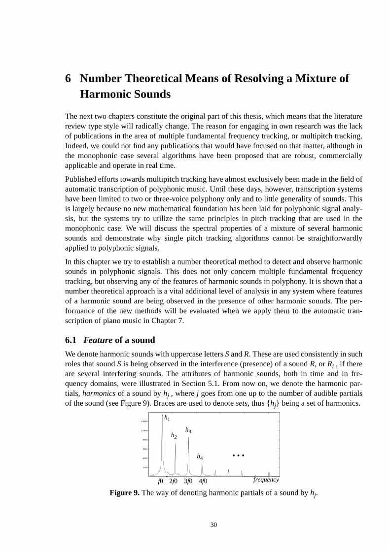
raturelack

ing.gh in

ercially

ld oftemsThisnaly-

n theonic

ardly

monicencyhat aturese per-tran-

h

n fre-par-

ls

6 Number Theoretical Means of Resolving a Mixture ofHarmonic Sounds

The next two chapters constitute the original part of this thesis, which means that the litereview type style will radically change. The reason for engaging in own research was theof publications in the area of multiple fundamental frequency tracking, or multipitch trackIndeed, we could not find any publications that would have focused on that matter, althouthe monophonic case several algorithms have been proposed that are robust, commapplicable and operate in real time.

Published efforts towards multipitch tracking have almost exclusively been made in the fieautomatic transcription of polyphonic music. Until these days, however, transcription syshave been limited to two or three-voice polyphony only and to little generality of sounds.is largely because no new mathematical foundation has been laid for polyphonic signal asis, but the systems try to utilize the same principles in pitch tracking that are used imonophonic case. We will discuss the spectral properties of a mixture of several harmsounds and demonstrate why single pitch tracking algorithms cannot be straightforwapplied to polyphonic signals.

In this chapter we try to establish a number theoretical method to detect and observe harsounds in polyphonic signals. This does not only concern multiple fundamental frequtracking, but observing any of the features of harmonic sounds in polyphony. It is shown tnumber theoretical approach is a vital additional level of analysis in any system where feaof a harmonic sound are being observed in the presence of other harmonic sounds. Thformance of the new methods will be evaluated when we apply them to the automaticscription of piano music in Chapter 7.

6.1 Featureof a sound

We denote harmonic sounds with uppercase lettersSandR. These are used consistently in sucroles that soundS is being observed in the interference (presence) of a soundR, or Ri , if thereare several interfering sounds. The attributes of harmonic sounds, both in time and iquency domains, were illustrated in Section 5.1. From now on, we denote the harmonictials, harmonicsof a sound byhj , wherej goes from one up to the number of audible partiaof the sound (see Figure 9). Braces are used to denotesets, thus {hj} being a set of harmonics.

0 50 100 150 200 250

200

400

600

800

1000

1200

frequency

Figure 9.The way of denoting harmonic partials of a sound byhj.

h1

h2h3

h4

f0 2f0 3f0 4f0

• • •

30

tently

e.

with aampli-g the

and alsolong toquires

artials,

f any ofthis is

s and. Thed to ad sev-

encyies.lopes

ed by

-

r-

Further, we denote byg(x) a featureof x, wherex can be a soundS,or its single harmonic par-tial hj. We will separate the different features by subscript characters, for example consisdenotinggF(x) the frequency ofx, gA(x) the amplitude ofx, andgL(x) the perceivable loudnessof x. Explanation and definition of each feature will be given when they are taken into us

We divide features g(x) into two classes, depending on whether they can be associatedsingle harmonic or not. Clearly, a single harmonic can have such features as frequency,tude, loudness and onset time, for example. This is the feature class I. To class II belonfeatures that can be applied to a sound, but are meaningless ifx is a single harmonichj . As anexample we considersound colour gC(S), which results from the distribution of the energy ofsound to its harmonics. Now, a single harmonic does not have such a feature as colour, acannot represent this feature of the sound alone. Thus the features of a sound that beclass I can be approximated by independent representative harmonics, but class II reobservation of the whole harmonic series as a single entity.

Because the very substance of a harmonic sound is its series of equidistant sinusoid pany observation of a harmonic sound must be based on its harmonic partials, since strictlyspeaking the sound has no other physical appearance than these partials. Calculation othe features of the sound must be based on the features of its harmonics, no matter ifdone in time or frequency domain.

6.2 The basic problem in resolving a mixture of harmonic sounds

There is a multitude of good methods for measuring the frequencies, amplitude envelopephases of sinusoid partials in a signal [McAulay86, Depalle93, Serra97, Ding97, Qian97]problem in resolving a mixture of harmonic sounds is that the harmonics of a sound extenwide frequency band, and most often the frequency bands of different sounds overlap, aneral harmonics of different sounds overlap. This causes two severe problems.

1. Because the harmonic series of different sounds typically extend to common frequbands, it is most difficult to assign the harmonics to their true fundamental frequenc

2. If two sinusoid partials overlap, i.e., have a common frequency, the amplitude enveand phases of the overlapping sinusoids can no longer be deduced from their sum.

These are the fundamental reasons why polyphonic signal contents cannot be resolvstraightforwardly applying the algorithms designed for monophonic signals.

Proposition 1. If any harmonic of a soundS is overlapped by any harmonic of an inter

fering soundR, then the fundamental frequency of the soundR must be , where

m andn are integer numbers greater than or equal to 1.

Proof. The frequency of a harmonic of the soundS is

(3)

and the frequency of a harmonic of the soundR is

The condition of a harmonic of a soundSto be overlapped by a harmonic of an interfeing soundR can be expressed as

, (4)

hjS

hiR

f 0Rmn---- f 0S⋅=

hjS

gF hjS( ) j f 0S⋅=

hiR

gF hiR( ) i f 0R⋅=

hjS

hiR

i f 0R⋅ j f 0S⋅= ) f 0Rji-- f 0S⋅=

⇔

31

undspro-where

ss

s pro-encystruc-

le the

l

al

when the common factors ofj andi are reduced, this can be expressed as

, (5)

where and can be calculated from the numbers of the harmonics,i andj. ❑

Comment. It may look as being a special case that the fundamental frequencies of two sowould have exactly this relation, but it is definitely not. This is due to the physics of soundduction and the rules governing fundamental frequencies of the notes in Western music,the fundamental frequencies of the notes most often have the abovementioned relation,mandnbeing small integers.

Proposition 2. If the fundamental frequencies of two harmonic soundsS andR are f0S and, respectively, then everynth harmonic of the soundR

overlaps a correspondingmth harmonic of the soundS.

Proof. Substituting (5) to (4) we can rewrite the condition of a harmonichj of a soundS to beoverlapped by a harmonichi of an interfering soundR as

,

which is true for each pairi=nk andj=mk, wherek={1, 2, 3, 4,...}.❑

Corollary. If the fundamental frequency of a soundR is , it will overlap all theharmonics of Sat their common frequency bands. OtherwiseR can overlap maximally everysecond harmonic ofS. If all harmonics ofSare overlapped by an interfering soundR, detectingthe two sounds is difficult and even theoretically ambiguous: the harmonics ofS might haveresulted fromR alone, and the soundS is easily undetected. On the other hand, if the loudneof the soundS is deliberately determined regardless of the soundR, Swill ‘steal’ the energy ofeverynth harmonic ofR to itself.

6.3 Certain principles in Western music

“Music transforms arithmetic relations into immediate sensations.”

-Schopenhauer, Metaphysics of Music

An important principle governing music is paying attention to the frequency relations,inter-vals, of simultaneously played notes. Here we use the word note to refer to a sound that iduced by a musical instrument. Paying attention to time intervals in rhythm and to frequintervals of concurrent sounds has a certain goal: to unify the sounds to form a coherentture that is able to express more than any of the sounds alone.

Two notes are in aharmonicrelation to each other if their fundamental frequencies satisfy

, (6)

wherem andn are small integers. The smaller the values ofm andn are, the closer is the har-

monic relation of the two sounds and the more perfectly they play together. For examp

fundamental frequencies , and constitute a basicmajor chord, and the fundamenta

frequencies , and constitute aminor chord. To read more about the mathematic

viewpoint to music, see [JIN98] and [Canright87].

f 0Rmn---- f 0S⋅=

m n,( ) 1≥

f 0Rmn---- f 0S⋅= hnk k, 1 2 3 4 …, , , ,=

hmk k, 1 2 3 4 …, , , ,=

i f 0R⋅ j f 0S⋅=( ) imn---- f 0S⋅ ⋅ j f 0S⋅=

i m⋅ j n⋅=( )⇔ ⇔

f 0R1n--- f 0S⋅=

f 02mn---- f 01⋅=

44--- f

54--- f

64--- f

46--- f

45--- f

44--- f

32

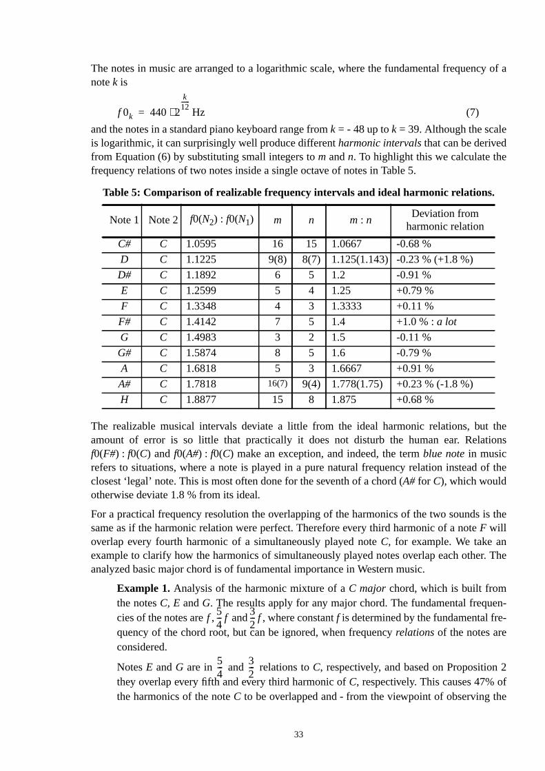
y of a

t theions

of the

is the

r. The

en--

2fhe

The notes in music are arranged to a logarithmic scale, where the fundamental frequencnotek is

Hz (7)

and the notes in a standard piano keyboard range fromk = - 48 up tok = 39. Although the scaleis logarithmic, it can surprisingly well produce differentharmonic intervalsthat can be derivedfrom Equation (6) by substituting small integers tom andn. To highlight this we calculate thefrequency relations of two notes inside a single octave of notes in Table 5.

The realizable musical intervals deviate a little from the ideal harmonic relations, buamount of error is so little that practically it does not disturb the human ear. Relatf0(F#) : f0(C) and f0(A#) : f0(C) make an exception, and indeed, the termblue notein musicrefers to situations, where a note is played in a pure natural frequency relation insteadclosest ‘legal’ note. This is most often done for the seventh of a chord (A# for C), which wouldotherwise deviate 1.8 % from its ideal.

For a practical frequency resolution the overlapping of the harmonics of the two soundssame as if the harmonic relation were perfect. Therefore every third harmonic of a noteF willoverlap every fourth harmonic of a simultaneously played noteC, for example. We take anexample to clarify how the harmonics of simultaneously played notes overlap each otheanalyzed basic major chord is of fundamental importance in Western music.

Example 1.Analysis of the harmonic mixture of aC major chord, which is built fromthe notesC, E andG. The results apply for any major chord. The fundamental frequcies of the notes are , and , where constantf is determined by the fundamental frequency of the chord root, but can be ignored, when frequencyrelationsof the notes areconsidered.

NotesE andG are in and relations toC, respectively, and based on Propositionthey overlap every fifth and every third harmonic ofC, respectively. This causes 47% othe harmonics of the noteC to be overlapped and - from the viewpoint of observing t

Table 5: Comparison of realizable frequency intervals and ideal harmonic relations.

Note 1 Note 2 f0(N2) : f0(N1) m n m: nDeviation from

harmonic relation

C# C 1.0595 16 15 1.0667 -0.68 %

D C 1.1225 9(8) 8(7) 1.125(1.143) -0.23 % (+1.8 %)

D# C 1.1892 6 5 1.2 -0.91 %

E C 1.2599 5 4 1.25 +0.79 %

F C 1.3348 4 3 1.3333 +0.11 %

F# C 1.4142 7 5 1.4 +1.0 % :a lot

G C 1.4983 3 2 1.5 -0.11 %

G# C 1.5874 8 5 1.6 -0.79 %

A C 1.6818 5 3 1.6667 +0.91 %

A# C 1.7818 16(7) 9(4) 1.778(1.75) +0.23 % (-1.8 %)

H C 1.8877 15 8 1.875 +0.68 %

f 0k 440 2

k12------

⋅=

f54--- f

32--- f

54--- 3

2---

33

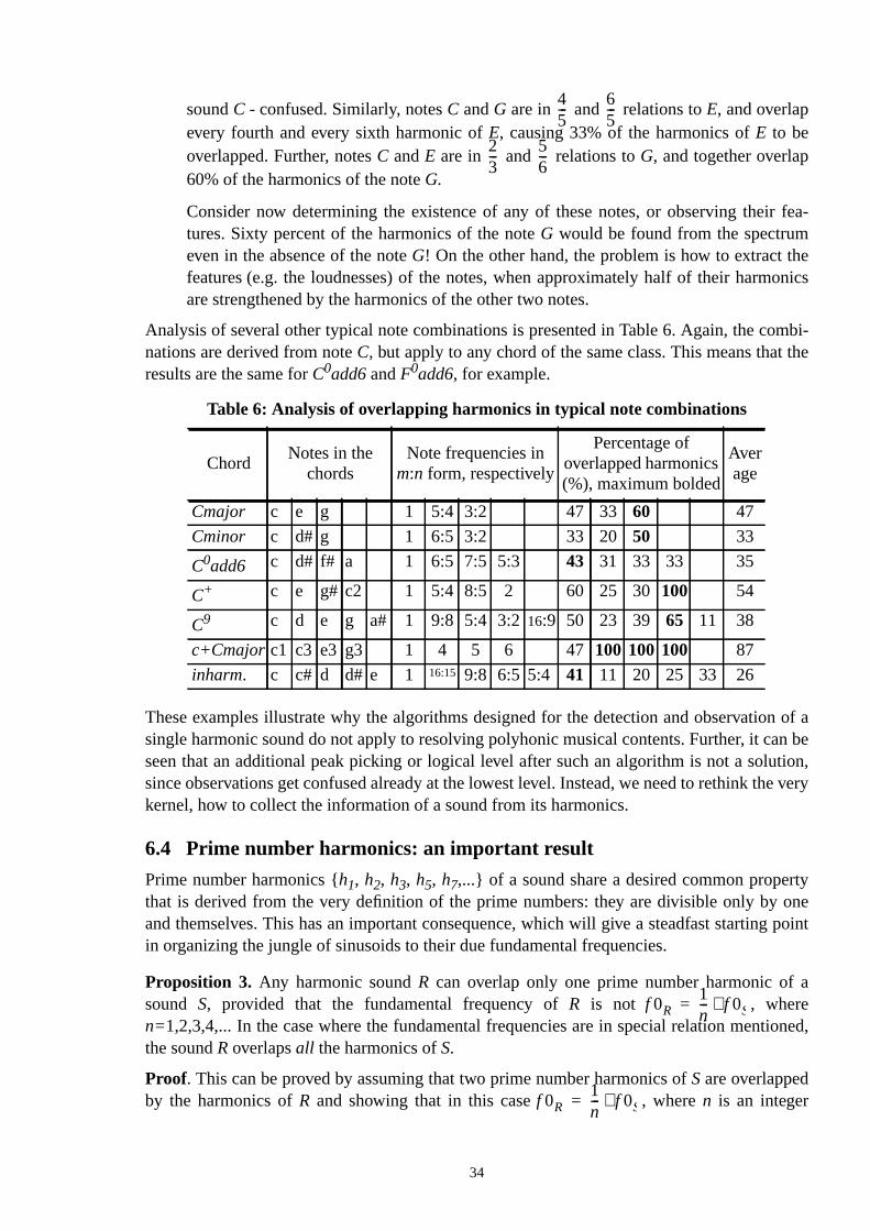
r fea-

eonics

mbi-the

n of an betion,e very

rtyonepoint

a

ioned,

soundC - confused. Similarly, notesC andG are in and relations toE, and overlapevery fourth and every sixth harmonic ofE, causing 33% of the harmonics ofE to beoverlapped. Further, notesC andE are in and relations toG, and together overlap60% of the harmonics of the noteG.

Consider now determining the existence of any of these notes, or observing theitures. Sixty percent of the harmonics of the noteG would be found from the spectrumeven in the absence of the noteG! On the other hand, the problem is how to extract thfeatures (e.g. the loudnesses) of the notes, when approximately half of their harmare strengthened by the harmonics of the other two notes.

Analysis of several other typical note combinations is presented in Table 6. Again, the conations are derived from noteC, but apply to any chord of the same class. This means thatresults are the same forC0add6 andF0add6, for example.

These examples illustrate why the algorithms designed for the detection and observatiosingle harmonic sound do not apply to resolving polyhonic musical contents. Further, it caseen that an additional peak picking or logical level after such an algorithm is not a solusince observations get confused already at the lowest level. Instead, we need to rethink thkernel, how to collect the information of a sound from its harmonics.

6.4 Prime number harmonics: an important result

Prime number harmonics {h1, h2, h3, h5, h7,...} of a sound share a desired common propethat is derived from the very definition of the prime numbers: they are divisible only byand themselves. This has an important consequence, which will give a steadfast startingin organizing the jungle of sinusoids to their due fundamental frequencies.

Proposition 3. Any harmonic soundR can overlap only one prime number harmonic ofsound S, provided that the fundamental frequency ofR is not , wheren=1,2,3,4,... In the case where the fundamental frequencies are in special relation mentthe soundR overlapsall the harmonics ofS.

Proof. This can be proved by assuming that two prime number harmonics ofSare overlappedby the harmonics ofR and showing that in this case , wheren is an integer

Table 6: Analysis of overlapping harmonics in typical note combinations

ChordNotes in the

chordsNote frequencies in

m:n form, respectively

Percentage ofoverlapped harmonics(%), maximum bolded

Average

Cmajor c e g 1 5:4 3:2 47 33 60 47

Cminor c d# g 1 6:5 3:2 33 20 50 33

C0add6 c d# f# a 1 6:5 7:5 5:3 43 31 33 33 35

C+ c e g# c2 1 5:4 8:5 2 60 25 30100 54

C9 c d e g a# 1 9:8 5:4 3:216:9 50 23 39 65 11 38

c+Cmajor c1 c3 e3 g3 1 4 5 6 47100 100 100 87

inharm. c c# d d# e 1 16:15 9:8 6:5 5:4 41 11 20 25 33 26

45--- 6

5---

23--- 5

6---

f 0R1n--- f 0S⋅=

f 0R1n--- f 0S⋅=

34

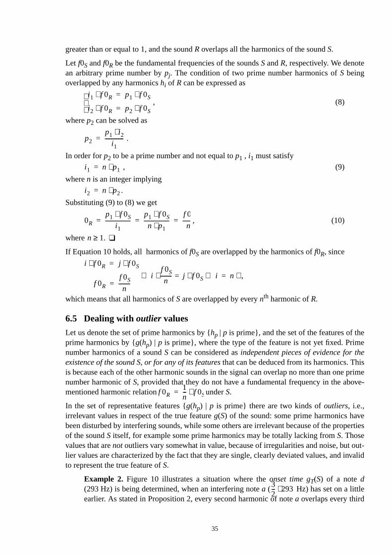
eeeisprimeve-

eperties

out-invalid

greater than or equal to 1, and the soundR overlaps all the harmonics of the soundS.

Let f0S andf0R be the fundamental frequencies of the soundsSandR, respectively. We denotean arbitrary prime number bypj. The condition of two prime number harmonics ofS beingoverlapped by any harmonicshi of R can be expressed as

, (8)

wherep2 can be solved as

.

In order forp2 to be a prime number and not equal top1 , i1 must satisfy

, (9)

wheren is an integer implying

.

Substituting (9) to (8) we get

, (10)

where ❑

If Equation 10 holds, all harmonics off0S are overlapped by the harmonics off0R, since

,

which means that all harmonics ofS are overlapped by everynth harmonic ofR.

6.5 Dealing withoutlier values

Let us denote the set of prime harmonics by {hp | p is prime}, and the set of the features of thprime harmonics by {g(hp) | p is prime}, where the type of the feature is not yet fixed. Primnumber harmonics of a soundS can be considered asindependent pieces of evidence for thexistence of the sound S, or for any of its featuresthat can be deduced from its harmonics. This because each of the other harmonic sounds in the signal can overlap no more than onenumber harmonic ofS, provided that they do not have a fundamental frequency in the abomentioned harmonic relation underS.

In the set of representative features {g(hp) | p is prime} there are two kinds ofoutliers, i.e.,irrelevant values in respect of the true featureg(S) of the sound: some prime harmonics havbeen disturbed by interfering sounds, while some others are irrelevant because of the proof the soundS itself, for example some prime harmonics may be totally lacking fromS. Thosevalues that arenotoutliers vary somewhat in value, because of irregularities and noise, butlier values are characterized by the fact that they are single, clearly deviated values, andto represent the true feature ofS.

Example 2. Figure 10 illustrates a situation where theonset time gT(S) of a noted(293 Hz) is being determined, when an interfering notea ( Hz) has set on a littleearlier. As stated in Proposition 2, every second harmonic of notea overlaps every third

i1 f 0R⋅ p1 f 0S⋅=

i2 f 0R⋅ p2 f 0S⋅=

p2

p1 i2⋅i1

--------------=

i1 n p1⋅=

i2 n p2⋅=

0R

p1 f 0S⋅i1

-------------------p1 f 0S⋅n p1⋅

-------------------f 0

n-------= = =

n 1.≥

i f 0R⋅ j f 0S⋅=

f 0R

f 0S

n---------=

i⇒f 0S

n---------⋅ j f 0S⋅= i⇔ n ⋅=

f 0R1n--- f 0S⋅=

32--- 293⋅

35

er-otermon-terfer-d 10

eIn this

thand.

nt theenta-e

feringture

se anad, thelynd onf the

ted set,rgest.

exam-sound

und.

harmonic of noted, but as stated in Proposition 3, only one prime harmonic is ovlapped, the third one. The sinusoids at the positions of the first ten harmonics of ndhave been indicated by lines, and the dots indicate their onset times. Overlapped haics 3 (prime), 6 and 9 are outliers, since onsets of these sinusoids are due to the ining notea, and propose all too early onset times. On the other hand, harmonics 8 anwere not detected, and represent all too late onset times, thus being outliers, too.

An analogous situation is met when e.g. theloudness gL(S) of a sound is being observed: somsingle prime harmonics have been overlapped by interfering sounds, and are outliers.case missing harmonics do not introduce true outliers - their loudness is just weakerexpected (zero), and are compensated by other harmonics that are louder than expecte

We are now faced with data in which several independent pieces of evidence represesame quantity. Some of them are corrupted, outlier values, but a majority of the represtives, calledsamples, are reliable, it being highly unprobable that a majority of the primnumber harmonics would be either missing or each corrupted by an independent intersound.This is the motivation for a design of a filter which would pick the estimated fea

from the set of independent representatives{ g(hp) | p is prime}, and drop out the irrele-vant values.

Consider taking the mean among the representatives,mean{ g(hp) | p is prime}. This is not sat-isfactory, since even one outlier in a set of, for example, seven prime harmonics will cauunacceptable deviation to the mean, since outlier values may be grossly erroneous. Insteclass ofmedian and order statistic filtersis prompted by the fact that they are particulareffective in dealing with the kind of data that we characterized above. These filters depesorting the set of representatives. In our previous Example 2, sorting the onset times oprime harmonics would result as depicted in Figure 11.

It can be seen that under- or overestimated outlier values map to the both ends of the sorand in between, the reliable representatives are sorted from the smallest up to the laBecause we can assume the majority of the values to be reliable, we can safely pick, forple, the middle (median) value of the sorted set. Thus we yield the desired feature of the

0 50 100 1500

5

10

15

20

25

time

log frequency

Figure 10.Determining the sound onset time in interference of an earlier started so

Notea sets on (interference).

Noted sets on.

g S( )

gT(h3) gT.(<missing harmonic>)

Figure 11.Outlier values map to the both ends of a sorted set of representatives.

small-valueoutliers

large-valueoutliers

reliable values

36

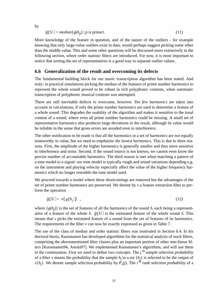
mpleotherin thet to

Andcs tomatic

ure oftonal

set ofwould

ually

nsitiveow thetern ofg e.g.har-

s of the

-

nics.

In hisfilters,ar fil-them

by

= median{ g(hp) | p is prime}. (11)

More knowledge of the feature in question, and of the nature of the outliers - for exaknowing that only large-value outliers exist in data, would perhaps suggest picking somethan the middle value. This and some other questions will be discussed more extensivelyfollowing section, where order statistic filters are introduced. For now, it is most importannotice that sorting the set of representatives is a good way to separate outlier values.

6.6 Generalization of the result and overcoming its defects

The fundamental building block for our music transcription algorithm has been stated.truly: in practical simulations picking the median of the features of prime number harmonirepresent the whole sound proved to be robust in rich polyphonic contents, when autotranscription of polyphonic musical contents was attempted.

There are still inevitable defects to overcome, however.Too few harmonicsare taken intoaccount in calculations, if only the prime number harmonics are used to determine a feata whole sound. This degrades the usability of the algorithm and makes it sensitive to thecontent of a sound, where even all prime number harmonics could be missing. A smallrepresentative harmonics also produces large deviations in the result, although its valuebe reliable in the sense that gross errors are avoided even in interference.

The other notification to be made is that all the harmonics in a set of harmonics are not eqtrustworthy in value, but we need toemphasize the lowest harmonics. This is due to three rea-sons. First, the amplitude of the higher harmonics is generally smaller and thus more seto interference and noise. Second, if the sound source is not known, we cannot even knprecise number of accountable harmonics. The third reason is met when matching a pata tone model to a signal: our tone model is typically rough and sound variations dependinon the instrument and playing velocity especially affect the value of the higher frequencymonics which no longer resemble the tone model used.

We proceed towards a model where these shortcomings are removed but the advantageset of prime number harmonics are preserved. We denote byv a feature extraction filter to per-form the operation

, (12)

where {g(hj)} is the set of features of all the harmonics of the soundS, each being a representative of a feature of the wholeS. is the estimated feature of the whole soundS. Thismeans thatv picks the estimated feature of a sound from the set of features of its harmoThe requirements of the filterv can now be exactly expressed as given in Table 7.

The use of the class of median and order statistic filters was motivated in Section 6.4.doctoral thesis, Kuosmanen has developed algorithms for the statistical analysis of stackcomprising the abovementioned filter classes plus an important portion of other non-lineters [Kuosmanen94, Astola97]. We implemented Kuosmanen’s algorithms, and will usein the continuation. First we need to define two concepts. Thej th sample selection probabilityof a filter v means the probability that the samplehj in a set {hj} is selected to be the output ofv{ hj}. We denote sample selection probability byPs(j). The i th rank selection probabilityof a

g S( )

g S( ) v g hj( ){ }=

g S( )

37

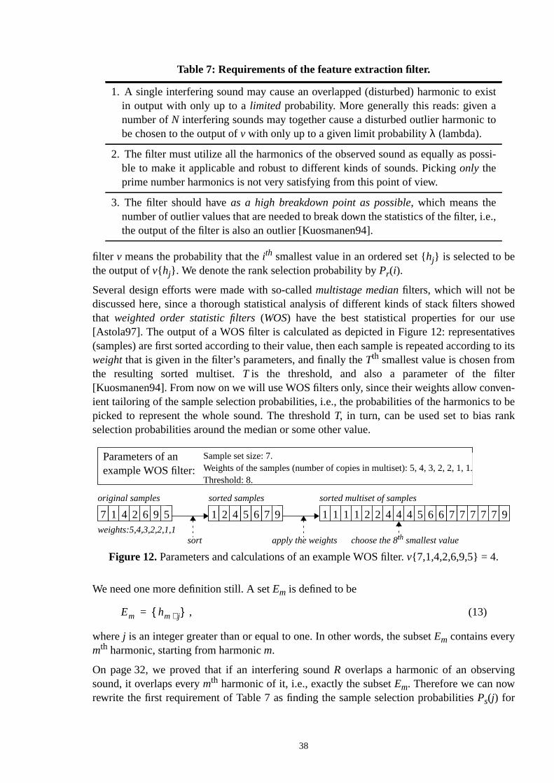
owedsetivesg to its

er

to bek

g

t

i-

.,

filter v means the probability that theith smallest value in an ordered set {hj} is selected to bethe output ofv{ hj}. We denote the rank selection probability byPr(i).

Several design efforts were made with so-calledmultistage medianfilters, which will not bediscussed here, since a thorough statistical analysis of different kinds of stack filters shthat weighted order statistic filters(WOS) have the best statistical properties for our u[Astola97]. The output of a WOS filter is calculated as depicted in Figure 12: representa(samples) are first sorted according to their value, then each sample is repeated accordinweightthat is given in the filter’s parameters, and finally theTth smallest value is chosen fromthe resulting sorted multiset.T is the threshold, and also a parameter of the filt[Kuosmanen94]. From now on we will use WOS filters only, since their weights allow conven-ient tailoring of the sample selection probabilities, i.e., the probabilities of the harmonicspicked to represent the whole sound. The thresholdT, in turn, can be used set to bias ranselection probabilities around the median or some other value.

We need one more definition still. A setEm is defined to be

, (13)

wherej is an integer greater than or equal to one. In other words, the subsetEm contains everymth harmonic, starting from harmonicm.

On page 32, we proved that if an interfering soundR overlaps a harmonic of an observinsound, it overlaps everymth harmonic of it, i.e., exactly the subsetEm. Therefore we can nowrewrite the first requirement of Table 7 as finding the sample selection probabilitiesPs(j) for

Table 7: Requirements of the feature extraction filter.

1. A single interfering sound may cause an overlapped (disturbed) harmonic to exisin output with only up to alimited probability. More generally this reads: given anumber ofN interfering sounds may together cause a disturbed outlier harmonic tobe chosen to the output ofv with only up to a given limit probabilityλ (lambda).

2. The filter must utilize all the harmonics of the observed sound as equally as possble to make it applicable and robust to different kinds of sounds. Pickingonly theprime number harmonics is not very satisfying from this point of view.

3. The filter should haveas a high breakdown point as possible, which means thenumber of outlier values that are needed to break down the statistics of the filter, i.ethe output of the filter is also an outlier [Kuosmanen94].

6 7 7 7 71111 54 422 64 7 971 5 942 67 1 4 592 6

Figure 12.Parameters and calculations of an example WOS filter.v{7,1,4,2,6,9,5} = 4.

original samples sorted samples sorted multiset of samples

Sample set size: 7.Weights of the samples (number of copies in multiset): 5, 4, 3, 2, 2, 1, 1.Threshold: 8.

Parameters of anexample WOS filter:

weights:5,4,3,2,2,1,1apply the weights choose the 8th smallest valuesort

Em hm j⋅{ }=

38

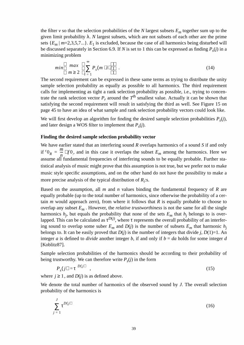
rimewill

e unitymentcen-t5 onk like.

er sta-

ake

ake a

cer-

r-

ty of

the filterv so that the selection probabilities of theN largest subsetsEm together sum up to thegiven limit probabilityλ. N largest subsets, which are not subsets of each other are the psets {Em | m=2,3,5,7...}.E1 is excluded, because the case of all harmonics being disturbedbe discussed separately in Section 6.9. IfN is set to 1 this can be expressed as findingPs(j) in aminimizing problem

. (14)

The second requirement can be expressed in these same terms as trying to distribute thsample selection probability as equally as possible to all harmonics. The third requirecalls for implementing as tight a rank selection probability as possible, i.e., trying to contrate the rank selection vectorPr around theTth smallest value. Actually it can be shown thasatisfying the second requirement will result in satisfying the third as well. See Figure 1page 45 to have an idea of what sample and rank selection probability vectors could loo

We will first develop an algorithm for finding the desired sample selection probabilitiesPs(j),and later design a WOS filter to implement thatPs(j).

Finding the desired sample selection probability vector

We have earlier stated that an interfering soundR overlaps harmonics of a soundS if and only

if , and in this case it overlaps the subsetEm among the harmonics. Here we

assume all fundamental frequencies of interfering sounds to be equally probable. Furth

tistical analysis of music might prove that this assumption is not true, but we prefer not to m

music style specific assumptions, and on the other hand do not have the possibility to m

more precise analysis of the typical distribution ofRi:s.

Based on the assumption, allm and n values binding the fundamental frequency ofR areequally probable (up to the total number of harmonics, since otherwise the probability of atain m would approach zero), from where it follows thatR is equally probable to choose tooverlap any subsetEm . However, therelative trustworthinessis not the same for all the singleharmonicshj, but equals the probability that none of the setsEm that hj belongs to is over-lapped. This can be calculated asτD(j), whereτ represents the overall probability of an interfeing sound to overlap some suberEm andD(j) is the number of subsetsEm that harmonichjbelongs to. It can be easily proved thatD(j) is the number of integers that dividej, D(1)=1. Anintegera is defined todivideanother integerb, if and only if b = da holds for some integerd[Koblitz87].

Sample selection probabilities of the harmonics should be according to their probabilibeing trustworthy. We can therefore writePs(j) in the form

, (15)

where , andD(j) is as defined above.

We denote the total number of harmonics of the observed sound byJ. The overall selectionprobability of the harmonics is

(16)

min max

m 2≥Ps m i⋅( )

i 1=

∞

∑

f 0Rmn---- f 0S⋅=

Ps j( ) τD j( )=

j 1≥

τD j( )

j 1=

J

∑

39

i-

y ofs in

ist.of

l

and should equal to unity.

SetI is defined to contain the numbersj of the harmonicshj that belong to some of theN larg-est subsets {Em | m=2,3,5,7...}. IfN=1, setI simply contains even numbers up toJ. The sumover the selection probabilities of the harmonics in theseN largest subsets is

. (17)

Finally, we can rewrite the first requirement of the feature exraction filterv (see Table 7 onpage 38) as

, (18)

from whichτ can be solved. Selection probabilitiesPs(j) can now be uniquely solved by substtuting τ to Equation 15.

The special properties of the resultingPs(j), and the role of the selectedλ value will be dis-cussed after representing the above reasoning in an algorithm form.

Algorithm 1. Calculation of the sample selection probabilitiesPs(j) of a feature extraction fil-ter v, so that the selection probability of a harmonic is according to its relative probabilitbeing trustworthy,τD(j), and so that the sum over the selection probabilities of the harmonicN largest subsets {Em | m=2,3,5,7...} yields the given limit probabilityλ. The sum over wholePs(j) is unity.

Step 1.CalculateD(j), wherej= 1,2,...,J, so thatD(j) is the number of positive integersthat dividej. This is the number of subsetsEm that a harmonichj belongs to.

Step 2.Form setI, which contains the numbersj of the harmonicshj that belong to someof theN largest subsets {Em | m=2,3,5,7...}. IfN = 1, setI simply contains even numbersup toJ.

Step 3.Setemax= max{D(j)}. Calculate vectorsA1(e) andA2(e), wheree=1,2,...,emax,so thatA1(e) = number of items inD(j) that satisfyD(j) = e

A2(e) = number of items in {D(j) | } that satisfyD(j) = e.Step 4.Form polynomial , where the coeffi-cientsae are .

Step 5.Find all roots of this polynomial by solvingf(τ)=0. Although this cannot be doneanalytically for higher than fourth order polynomials, efficient numerical methods exIn practice, this reduces to finding eigenvalues of the associated companion matrixA[Horn85].

Step 6.If the problem is solvable for givenN, λ andJ, there is only one root that is reaand between 0 and 1. This root is the valueτ that was discussed earlier.

Step 7.Calculate an initial sample selection probability vector of the WOS filter as

.

Step 8.Divide each value by to scale its sum to unity. This isPs(j).

τD j( )

j I∈∑

τD j( )

j I∈∑ λ τD j( )

j 1=

J

∑⋅=

j I∈f τ( ) a1 τ a2 τ2 …+⋅ aemax τemax⋅+ +⋅=

ae A2 e( ) λ A1 e( )⋅( )–=

PSˆ j( ) τ( )D j( )

=

Ps j( ) Ps j( )∑

40

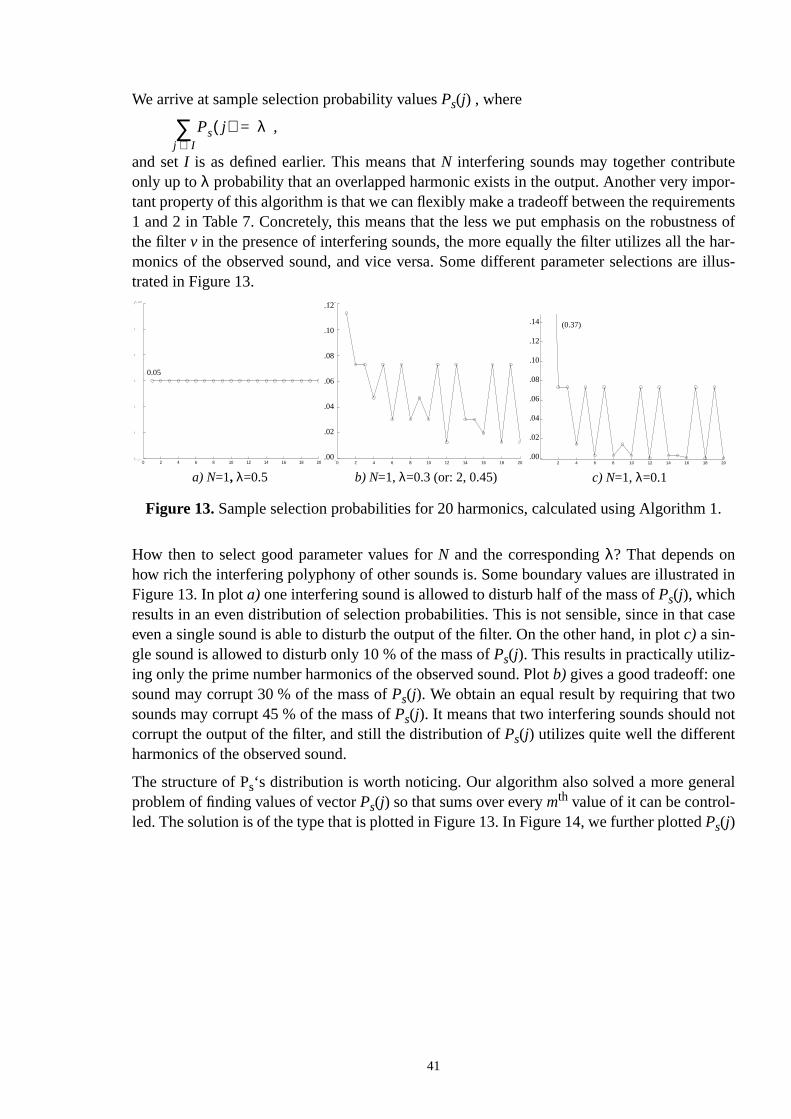
eor-entsess of

har-e illus-

ed in

case

oot

ral

1.

We arrive at sample selection probability valuesPs(j) , where

,

and setI is as defined earlier. This means thatN interfering sounds may together contributonly up toλ probability that an overlapped harmonic exists in the output. Another very imptant property of this algorithm is that we can flexibly make a tradeoff between the requirem1 and 2 in Table 7. Concretely, this means that the less we put emphasis on the robustnthe filterv in the presence of interfering sounds, the more equally the filter utilizes all themonics of the observed sound, and vice versa. Some different parameter selections artrated in Figure 13.

How then to select good parameter values forN and the correspondingλ? That depends onhow rich the interfering polyphony of other sounds is. Some boundary values are illustratFigure 13. In plota) one interfering sound is allowed to disturb half of the mass ofPs(j), whichresults in an even distribution of selection probabilities. This is not sensible, since in thateven a single sound is able to disturb the output of the filter. On the other hand, in plotc) a sin-gle sound is allowed to disturb only 10 % of the mass ofPs(j). This results in practically utiliz-ing only the prime number harmonics of the observed sound. Plotb) gives a good tradeoff: onesound may corrupt 30 % of the mass ofPs(j). We obtain an equal result by requiring that twsounds may corrupt 45 % of the mass ofPs(j). It means that two interfering sounds should ncorrupt the output of the filter, and still the distribution ofPs(j) utilizes quite well the differentharmonics of the observed sound.

The structure of Ps‘s distribution is worth noticing. Our algorithm also solved a more geneproblem of finding values of vectorPs(j) so that sums over everymth value of it can be control-led. The solution is of the type that is plotted in Figure 13. In Figure 14, we further plottedPs(j)

Ps j( )j I∈∑ λ=

a) N=1, λ=0.5 b) N=1, λ=0.3 (or: 2, 0.45) c) N=1, λ=0.10 2 4 6 8 10 12 14 16 18 20

0.05

0.05

0.05

0.05

0.05

0.05

0.05

0 2 4 6 8 10 12 14 16 18 200

0.02

0.04

0.06

0.08

0.1

0.12

2 4 6 8 10 12 14 16 18 200

0.02

0.04

0.06

0.08

0.1

0.12

0.14

Figure 13.Sample selection probabilities for 20 harmonics, calculated using Algorithm

(0.37)

.12

.10

.08

.06

.04

.02

.00

.14

.12

.10

.08

.06

.04

.02

.00

0.05

41

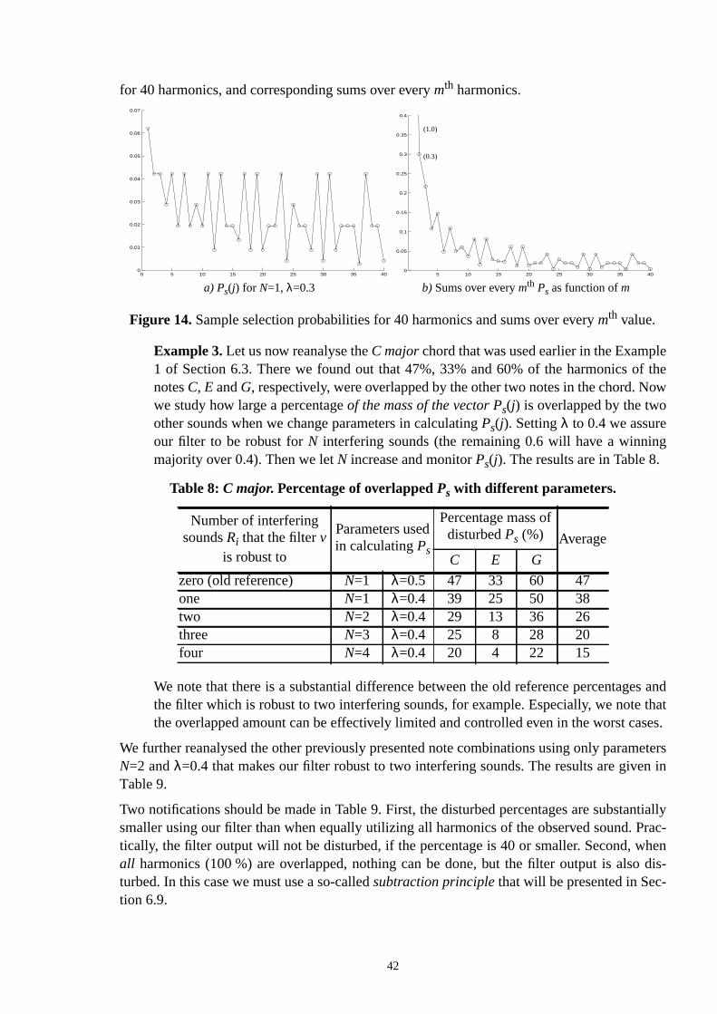
lef theow

g

es andthatases.

metersn in

ntiallyrac-hendis-

for 40 harmonics, and corresponding sums over everymth harmonics.

Example 3.Let us now reanalyse theC majorchord that was used earlier in the Examp1 of Section 6.3. There we found out that 47%, 33% and 60% of the harmonics onotesC, E andG, respectively, were overlapped by the other two notes in the chord. Nwe study how large a percentageof the mass of the vector Ps(j) is overlapped by the twoother sounds when we change parameters in calculatingPs(j). Settingλ to 0.4 we assureour filter to be robust forN interfering sounds (the remaining 0.6 will have a winninmajority over 0.4). Then we letN increase and monitorPs(j). The results are in Table 8.

We note that there is a substantial difference between the old reference percentagthe filter which is robust to two interfering sounds, for example. Especially, we notethe overlapped amount can be effectively limited and controlled even in the worst c

We further reanalysed the other previously presented note combinations using only paraN=2 andλ=0.4 that makes our filter robust to two interfering sounds. The results are giveTable 9.

Two notifications should be made in Table 9. First, the disturbed percentages are substasmaller using our filter than when equally utilizing all harmonics of the observed sound. Ptically, the filter output will not be disturbed, if the percentage is 40 or smaller. Second, wall harmonics (100 %) are overlapped, nothing can be done, but the filter output is alsoturbed. In this case we must use a so-calledsubtraction principlethat will be presented in Sec-tion 6.9.

Table 8: C major. Percentage of overlappedPs with different parameters.

Number of interferingsoundsRi that the filterv

is robust to

Parameters usedin calculatingPs

Percentage mass ofdisturbedPs (%) Average

C E G

zero (old reference) N=1 λ=0.5 47 33 60 47one N=1 λ=0.4 39 25 50 38two N=2 λ=0.4 29 13 36 26three N=3 λ=0.4 25 8 28 20four N=4 λ=0.4 20 4 22 15

0 5 10 15 20 25 30 35 400

0.01

0.02

0.03

0.04

0.05

0.06

0.07

5 10 15 20 25 30 35 400

0.05

0.1

0.15

0.2

0.25

0.3

0.35

0.4

(1.0)

a) Ps(j) for N=1, λ=0.3 b) Sums over everymth Ps as function ofm

Figure 14.Sample selection probabilities for 40 harmonics and sums over everymth value.

(0.3)

42

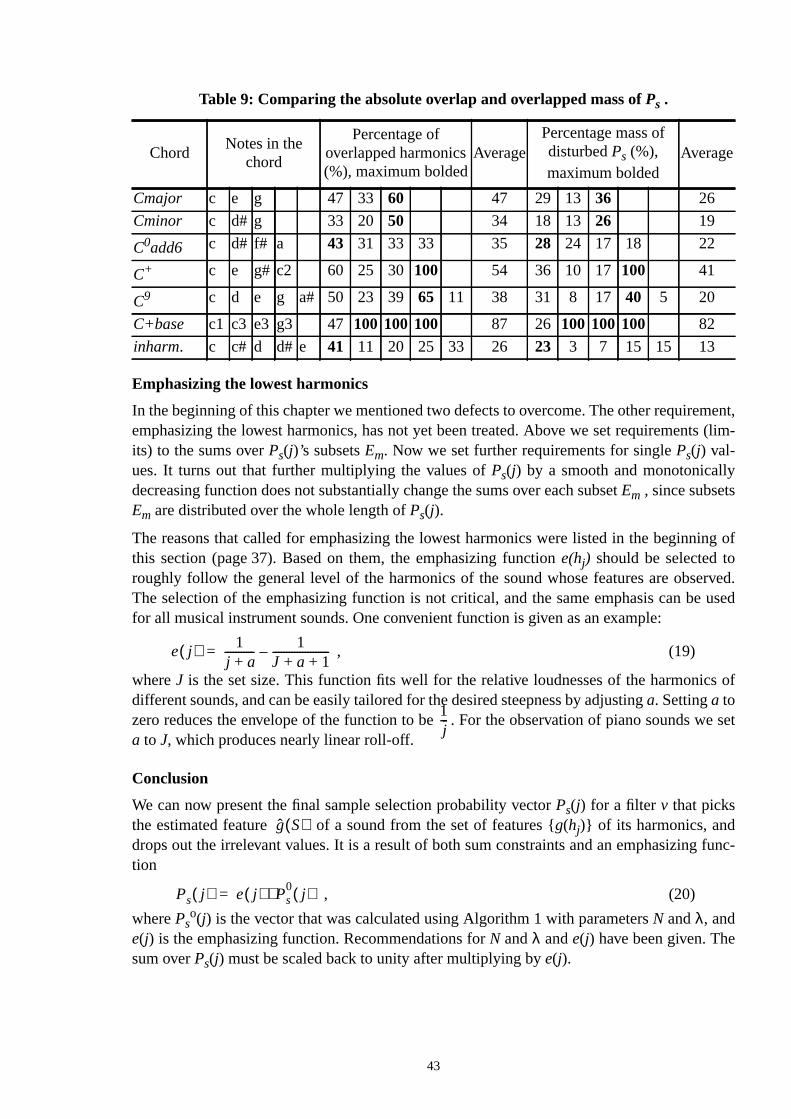
ment,s (lim-

ing of

rved.used

s of

we set

func-

Emphasizing the lowest harmonics

In the beginning of this chapter we mentioned two defects to overcome. The other requireemphasizing the lowest harmonics, has not yet been treated. Above we set requirementits) to the sums overPs(j)’s subsetsEm. Now we set further requirements for singlePs(j) val-ues. It turns out that further multiplying the values ofPs(j) by a smooth and monotonicallydecreasing function does not substantially change the sums over each subsetEm , since subsetsEm are distributed over the whole length ofPs(j).

The reasons that called for emphasizing the lowest harmonics were listed in the beginnthis section (page 37). Based on them, the emphasizing functione(hj) should be selected toroughly follow the general level of the harmonics of the sound whose features are obseThe selection of the emphasizing function is not critical, and the same emphasis can befor all musical instrument sounds. One convenient function is given as an example:

, (19)

whereJ is the set size. This function fits well for the relative loudnesses of the harmonicdifferent sounds, and can be easily tailored for the desired steepness by adjustinga. Settinga tozero reduces the envelope of the function to be . For the observation of piano soundsa to J, which produces nearly linear roll-off.

Conclusion

We can now present the final sample selection probability vectorPs(j) for a filter v that picksthe estimated feature of a sound from the set of features {g(hj)} of its harmonics, anddrops out the irrelevant values. It is a result of both sum constraints and an emphasizingtion

, (20)

wherePso(j) is the vector that was calculated using Algorithm 1 with parametersN andλ, and

e(j) is the emphasizing function. Recommendations forN andλ ande(j) have been given. Thesum overPs(j) must be scaled back to unity after multiplying bye(j).

Table 9: Comparing the absolute overlap and overlapped mass ofPs .

ChordNotes in the

chord

Percentage ofoverlapped harmonics(%), maximum bolded

AveragePercentage mass ofdisturbedPs (%),maximum bolded

Average

Cmajor c e g 47 33 60 47 29 13 36 26

Cminor c d# g 33 20 50 34 18 13 26 19

C0add6 c d# f# a 43 31 33 33 35 28 24 17 18 22

C+ c e g# c2 60 25 30100 54 36 10 17 100 41

C9 c d e g a# 50 23 3965 11 38 31 8 17 40 5 20

C+base c1 c3 e3 g3 47100 100 100 87 26 100 100 100 82

inharm. c c# d d# e 41 11 20 25 33 26 23 3 7 15 15 13

e j( ) 1j a+----------- 1

J a 1+ +---------------------–=

1j---

g S( )

Ps j( ) e j( ) Ps0

j( )⋅=

43

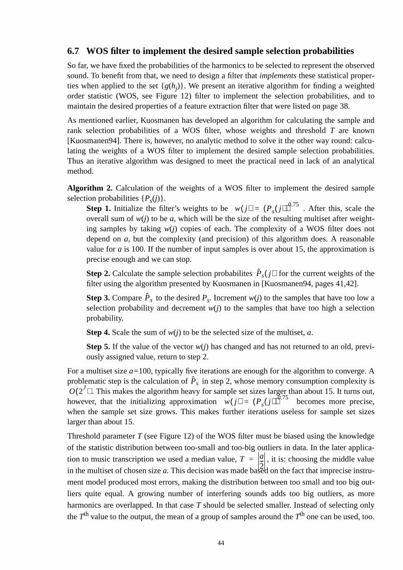
served

dd to

le and

alcu-ities.ytical

ple

et-otblen is

the].

aon

vi-

. Aity iss out,ise,t sizes

dge

lica-

alue

tru-

out-

ore

nly

.

6.7 WOS filter to implement the desired sample selection probabilities

So far, we have fixed the probabilities of the harmonics to be selected to represent the obsound. To benefit from that, we need to design a filter thatimplementsthese statistical proper-ties when applied to the set {g(hj)}. We present an iterative algorithm for finding a weighteorder statistic (WOS, see Figure 12) filter to implement the selection probabilities, anmaintain the desired properties of a feature extraction filter that were listed on page 38.

As mentioned earlier, Kuosmanen has developed an algorithm for calculating the samprank selection probabilities of a WOS filter, whose weights and thresholdT are known[Kuosmanen94]. There is, however, no analytic method to solve it the other way round: clating the weights of a WOS filter to implement the desired sample selection probabilThus an iterative algorithm was designed to meet the practical need in lack of an analmethod.

Algorithm 2. Calculation of the weights of a WOS filter to implement the desired samselection probabilities {Ps(j)}.

Step 1. Initialize the filter’s weights to be . After this, scale thoverall sum ofw(j) to bea, which will be the size of the resulting multiset after weighing samples by takingw(j) copies of each. The complexity of a WOS filter does ndepend ona, but the complexity (and precision) of this algorithm does. A reasonavalue fora is 100. If the number of input samples is over about 15, the approximatioprecise enough and we can stop.

Step 2.Calculate the sample selection probabilites for the current weights offilter using the algorithm presented by Kuosmanen in [Kuosmanen94, pages 41,42

Step 3.Compare to the desiredPs. Incrementw(j) to the samples that have too lowselection probability and decrementw(j) to the samples that have too high a selectiprobability.

Step 4.Scale the sum ofw(j) to be the selected size of the multiset,a.

Step 5.If the value of the vectorw(j) has changed and has not returned to an old, preously assigned value, return to step 2.

For a multiset sizea=100, typically five iterations are enough for the algorithm to convergeproblematic step is the calculation of in step 2, whose memory consumption complex

. This makes the algorithm heavy for sample set sizes larger than about 15. It turnhowever, that the initializing approximation becomes more precwhen the sample set size grows. This makes further iterations useless for sample selarger than about 15.

Threshold parameterT (see Figure 12) of the WOS filter must be biased using the knowle

of the statistic distribution between too-small and too-big outliers in data. In the later app

tion to music transcription we used a median value, , it is: choosing the middle v

in the multiset of chosen sizea. This decision was made based on the fact that imprecise ins

ment model produced most errors, making the distribution between too small and too big

liers quite equal. A growing number of interfering sounds adds too big outliers, as m

harmonics are overlapped. In that caseT should be selected smaller. Instead of selecting o

theTth value to the output, the mean of a group of samples around theTth one can be used, too

w j( ) Ps j( )( )0.75=

Ps j( )

Ps

Ps

O 2J( )

w j( ) Ps j( )( )0.75=

T a2---=

44

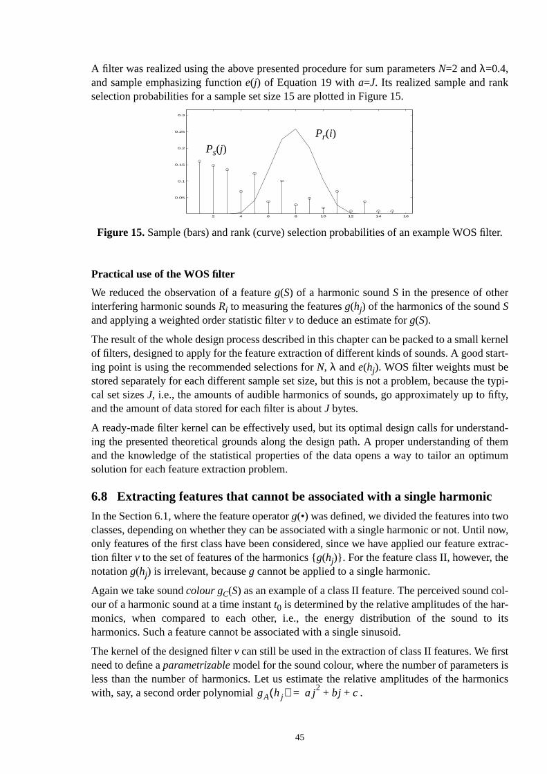
kerneltart-

e typi-fifty,

tand-f themimum

oil now,extrac-

col-r-

to its

rsts isonics

lter.

A filter was realized using the above presented procedure for sum parametersN=2 andλ=0.4,and sample emphasizing functione(j) of Equation 19 witha=J. Its realized sample and rankselection probabilities for a sample set size 15 are plotted in Figure 15.

Practical use of the WOS filter

We reduced the observation of a featureg(S) of a harmonic soundS in the presence of otherinterfering harmonic soundsRi to measuring the featuresg(hj) of the harmonics of the soundSand applying a weighted order statistic filterv to deduce an estimate forg(S).

The result of the whole design process described in this chapter can be packed to a smallof filters, designed to apply for the feature extraction of different kinds of sounds. A good sing point is using the recommended selections forN, λ ande(hj). WOS filter weights must bestored separately for each different sample set size, but this is not a problem, because thcal set sizesJ, i.e., the amounts of audible harmonics of sounds, go approximately up toand the amount of data stored for each filter is aboutJ bytes.

A ready-made filter kernel can be effectively used, but its optimal design calls for undersing the presented theoretical grounds along the design path. A proper understanding oand the knowledge of the statistical properties of the data opens a way to tailor an optsolution for each feature extraction problem.

6.8 Extracting features that cannot be associated with a single harmonic

In the Section 6.1, where the feature operatorg(•) was defined, we divided the features into twclasses, depending on whether they can be associated with a single harmonic or not. Untonly features of the first class have been considered, since we have applied our featuretion filter v to the set of features of the harmonics {g(hj)}. For the feature class II, however, thenotationg(hj) is irrelevant, becauseg cannot be applied to a single harmonic.

Again we take soundcolour gC(S) as an example of a class II feature. The perceived soundour of a harmonic sound at a time instantt0 is determined by the relative amplitudes of the hamonics, when compared to each other, i.e., the energy distribution of the soundharmonics. Such a feature cannot be associated with a single sinusoid.

The kernel of the designed filterv can still be used in the extraction of class II features. We fineed to define aparametrizablemodel for the sound colour, where the number of parameterless than the number of harmonics. Let us estimate the relative amplitudes of the harmwith, say, a second order polynomial .

2 4 6 8 10 12 14 16

0.05

0.1

0.15

0.2

0.25

0.3

Ps(j)

Pr(i)

Figure 15.Sample (bars) and rank (curve) selection probabilities of an example WOS fi

gA hj( ) a j2

bj c+ +=

45

to the

aluesr overd-

tionsl opti-

nsof af the

nce of

t: thethis iscussed

d

lower

be pre-in the

rtion

this

all its

allysingle

Now extracting this model’s parameters from the observed signal in a manner analogousWOS filtering is an optimization problem. We need to determine the parametersa, b andc sothat L1 error, i.e., the absolute value of the difference between the model’s amplitude vand the values of the actual harmonics in the spectrum is minimized. Further, the L1-errothe sample points must be taken as aweightedsum, where the weight of each sample is accoring to the sample selection probabilitiesPs(j). The meaning of the thresholdT of the filter canbe taken into account by giving a different emphasis to the positive and negative deviafrom the actual sample values. Fitting a function to datapoints in L1 sense is quite a usuamization problem, and is not treated here.

Adaptive instrument modelingis a problem to be solved using this kind of procedure. It meathe problem of finding the colour of a tone (sound of a musical instrument) from the midstpolyphonic piece of music by adapting the model’s parameters along with the playing opiece.

6.9 Feature ‘subtraction’ principle

Our algorithm and discussion on the observation of the features of sounds in the preseother harmonic sounds was based on an assumption that the observed soundS is not totallyoverlapped by an interfering sound R, whose fundamental frequency is

.

As a last case, we will now propose a method for dishing up this worst case. To repeaobserved sound is totally buried under the harmonics of an interfering sound, and evennot an extremely special situation, because of the characteristics of music that were disin Section 6.3.

The basic idea of our solution is tocompensatethe effect of the interfering soundR, the prop-erties of which can be robustly extracted in the presence ofS using the procedure presentebefore, because the interfering sound is not totally overlapped byS. Thus it will be enough todevelop an algorithm to subtract, remove, or compensate, the revealed properties of thesound and then proceed to determine the properties of the soundS, which is laid bare fromunder the interfering sound.

The subtraction process crucially depends on the feature under inspection, and cannotsented in a general form. Instead, we treat one example that has often been discussedfield of automatic transcription of polyphonic music [Chafe85, Brown91b, Martin96a,b].

Example 4. The problem is to determine the hypotheticalexistenceand loudnessof asoundSat the fundamental frequencyf0s, which has been totally overlapped by a lowesound, whose fundamental frequency is in the aforementioned relato S.

The existence of the lower soundR can be deduced using the methods presented inchapter. Moreover, its loudnessgL(R) is robustly determined in spite of everynth har-monic being overlapped by the soundS. But for the soundS it is most difficult to deter-mine whether it even exists (not to speak about recovering its loudness), becauseharmonics are overlapped by the harmonics of the soundR and could therefore beresulted from the soundR alone. The existence of the sound S is indeed theoreticambiguous because the same signal content could really have been resulted from a

f 0R1n--- f 0S⋅=

f 0R1n--- f 0S⋅=

46

s in a

oftically

n

corre-

roughef thein

rmedtran-

cyts

robusteven

t one,

harmonic sound having stronger harmonics at everynth positions.

There is, however, a remedy to the problem of detecting the higher one of the two soundharmonic relation to each other. The higher sound is revealed by theregularity at which theamplitudes of the harmonics at everynth positions exceed the overall level of the harmonicsR. Although this cue is theoretically ambiguous, as stated above, it is both psychoacousrelevant and practically useful.

The principal problem in subtracting the harmonics ofR from the spectrum is that although aestimate of the featuregL(R) can be deduced from the features {gL(hj)} of its harmonics, thiscannot be done vice versa, i.e., {gL(hj)} cannot be precisely deduced fromgL(R), although itwould be desirable to enable subtracting the loudness of each single harmonic from thesponding sinusoid in the spectrum.

We approximate subtracting, however. Some parametrizable curve is fitted in L1 sense ththe spectrum peaks at the slots of the harmonic partials ofR.This is done using the procedurpresented in Section 6.8. Now this curve determines the approximated distribution orobustly calculated loudness ofR to its harmonics. It turns out that the approximation madethe loudness distribution does not crucially change the loudness ofS, when determined afterthe subtraction. Subtracting a set of sinusoids from a Hamming windowed Fourier transfospectrum is another story altogether, and will be explained, when our automatic musicscriber is considered in the next chapter.

After the sinusoid partials of the soundRare removed, we notice that a fundamental frequencandidate ofSat the position of thenth harmonic ofR stands naked in the spectrum. When iloudness is determined using the same procedure as forR, it turns out that the soundS trulyexists, because it is loud enough to be heard as an independent sound. It is seen that adetermination of the loudness of the lower sound gives a steady ground to approachtotally overlapping set of potential sound candidates in a signal by starting from the lowesdetermining its loudness, subtracting it, and continuing upwards to the next candidate.

47

pply-.

tran-differ-d all

ayedand toithout

retical

tion. Weeflect

s ofl, bute usely usebina-

of theknowreli-

stemo try

re two

on ofreafternedeter-

7 Applying the New Method to the AutomaticTranscription of Polyphonic Music

In this chapter we evaluate and verify the theoretical results of the previous chapter by aing them in a computer program whose purpose is to transcribe polyphonic piano music

The challenge to our system is shortly stated as follows. We take the instrument to bescribed and record its different notes one by one, a sufficient amount to represent all theenttone coloursthat can be produced by that instrument. In the case of a piano we recordeits keys one at a time. This is what we calltraining material. When our program has studiedthe training material we require that it can transcribe rich polyphonic musical signals plwith the same instrument, i.e., to decompose signals into a subset of training set tonesdetermine their loudnesses and fundamental frequencies in the signal. Transcribing wtraining material will be discussed, too.

This is a good simulation arrangement to evaluate the efficiency of the presented theomethods in resolving a mixture of harmonic sounds. Emphasis is laid on resolvingrich poly-phonic contentsthat have been previously impossible to transcribe. We will present simularesults both for ‘typical stumbling point’ note mixtures and for classic piano compositionswill also compare this transcription system to our older pattern recognition approach, rtheir differences and strengths, and evaluate the role of the new methods.

7.1 Approach and design philosophy

Music transcription is a complicated cognitive task and requires integration of various formknowledge. A human listener not only uses the information that is present in the signaalso utilizes his prior knowledge about musical conventions and instrument tones. Here wa so-called bottom-up approach only, which means we ignore musical knowledge and onthe information that can be found from the recorded signals. In other words, all note comtions and sequences are assumed equally probable.

In Section 3.6 we presented a certain design philosophy, which goes through the designsystem as a background flow of thought. Shortly, at each abstraction level we must firstwhat information is needed, then find the best method to extract it, and finally analyse theability of the measurements. This philosophy has by far determined the selection of sybuilding blocks from among the tools presented in literature. An additional objective was tto concentrate on algorithm design and to avoid spending time on parameter tuning.

7.2 Overview of the system

Overview of the system is presented in Figure 16. It consists of three processes, whesupporting processes pass their results to atranscription processin the middle. Output fromstudying the training material is a bank of tone models, that is, the parametrized informatithe tones that may exist in signals that should be transcribed. The studying process is hecalledtone model creation process.It makes a radical assumption that only one musical toplays at a time in the training material and then proceeds by segmenting the signal and

48

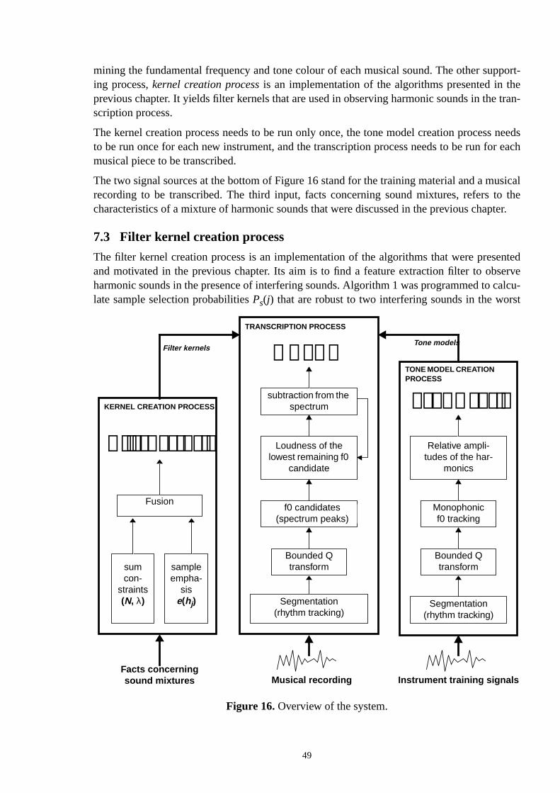
pport-hetran-

needsr each

usicalo thepter.

entederve

calcu-st

mining the fundamental frequency and tone colour of each musical sound. The other suing process,kernel creation processis an implementation of the algorithms presented in tprevious chapter. It yields filter kernels that are used in observing harmonic sounds in thescription process.

The kernel creation process needs to be run only once, the tone model creation processto be run once for each new instrument, and the transcription process needs to be run fomusical piece to be transcribed.

The two signal sources at the bottom of Figure 16 stand for the training material and a mrecording to be transcribed. The third input, facts concerning sound mixtures, refers tcharacteristics of a mixture of harmonic sounds that were discussed in the previous cha

7.3 Filter kernel creation process

The filter kernel creation process is an implementation of the algorithms that were presand motivated in the previous chapter. Its aim is to find a feature extraction filter to obsharmonic sounds in the presence of interfering sounds. Algorithm 1 was programmed tolate sample selection probabilitiesPs(j) that are robust to two interfering sounds in the wor

Tone models

Bounded Qtransform

f0 candidates(spectrum peaks)

Loudness of thelowest remaining f0

candidate

Musical recording Instrument training signals

subtraction from thespectrum

Bounded Qtransform

Monophonicf0 tracking

Relative ampli-tudes of the har-

monics

NOTES

Tone models

TRANSCRIPTION PROCESS

TONE MODEL CREATIONPROCESS

KERNEL CREATION PROCESS

Filter kernels

sampleempha-

sise(hj)

sumcon-

straints(N, λ)

Facts concerningsound mixtures

Fusion

Segmentation(rhythm tracking)

Segmentation(rhythm tracking)

Figure 16.Overview of the system.

Filter kernels

49

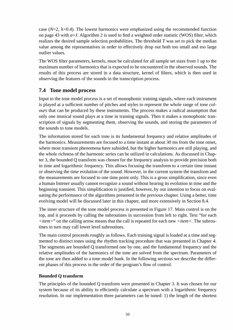
ctionch

large

to thes. Theed in

ument

ion thattran-ters of

es ofonset,g, and

Chap-n bothtantandeven

d theval-r, time4.

n theeach

seg-pter 4.and theters ofdiffer-

or ourencyortest

case (N=2, λ=0.4). The lowest harmonics were emphasized using the recommended funon page 43 witha=J. Algorithm 2 is used to find a weighted order statistic (WOS) filter, whirealizes the desired sample selection probabilities. The thresholdT was set to pick the medianvalue among the representatives in order to effectively drop out both too small and toooutlier values.

The WOS filter parameters, kernels, must be calculated for all sample set sizes from 1 upmaximum number of harmonics that is expected to be encountered in the observed soundresults of this process are stored in a data structure, kernel of filters, which is then usobserving the features of the sounds in the transcription process.

7.4 Tone model process

Input to the tone model process is a set of monophonic training signals, where each instris played at a sufficient number of pitches and styles to represent the whole range oftone col-ours that can be produced by these instruments. The process makes a radical assumptonly one musical sound plays at a time in training signals. Then it makes a monophonicscription of signals by segmenting them, observing the sounds, and storing the paramethe sounds to tone models.

The information stored for each tone is its fundamental frequency and relative amplitudthe harmonics. Measurements are focused to a time instant at about 30 ms from the tonewhere most transient phenomena have subsided, but the higher harmonics are still playinthe whole richness of the harmonic series can be utilized in calculations. As discussed inter 3, the bounded Q transform was chosen for the frequency analysis to provide precisioin time and logarithmic frequency. This allows focusing the transform to a certain time insor observing the time evolution of the sound. However, in the current system the transformthe measurements are focused to one time point only. This is a gross simplification, sincea human listener usually cannot recognize a sound without hearing its evolution in time anbeginning transient. This simplification is justified, however, by our intention to focus on euating the performance of the algorithms presented in the previous chapter. Using a betteevolving model will be discussed later in this chapter, and more extensively in Section 8.

The inner structure of the tone model process is presented in Figure 17. Main control is otop, and it proceeds by calling the subroutines in succession from left to right. Text “for<item>” on the calling arrow means that the call is repeated for each new<item>. The subrou-tines in turn may call lower level subroutines.

The main control proceeds roughly as follows. Each training signal is loaded at a time andmented to distinct tones using the rhythm tracking procedure that was presented in ChaThe segments are bounded Q transformed one by one, and the fundamental frequencyrelative amplitudes of the harmonics of the tone are solved from the spectrum. Paramethe tone are then added to a tone model bank. In the following sections we describe theent phases of this process in the order of the program’s flow of control.

Bounded Q transform

The principles of the bounded Q transform were presented in Chapter 3. It was chosen fsystem because of its ability to efficiently calculate a spectrum with a logarithmic frequresolution. In our implementation three parameters can be tuned: 1) the length of the sh

50

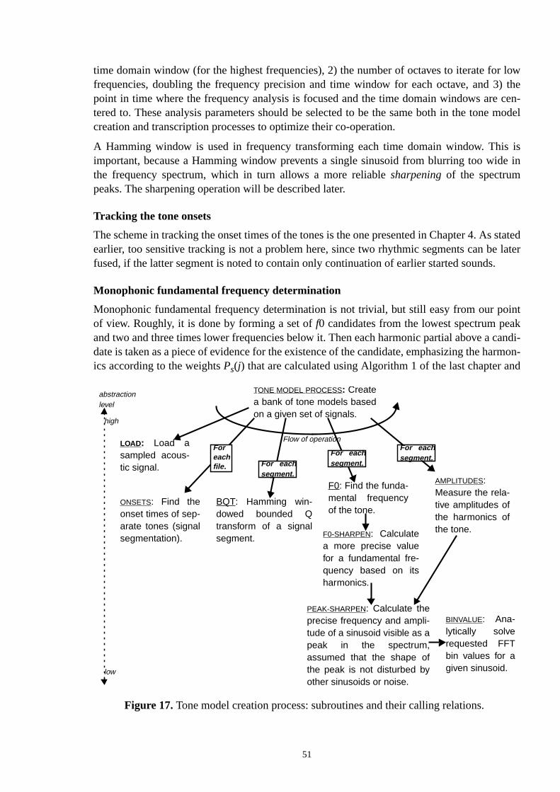
r low) thecen-model

s ise in

statedlater

.

ointakcandi-armon-nd

time domain window (for the highest frequencies), 2) the number of octaves to iterate fofrequencies, doubling the frequency precision and time window for each octave, and 3point in time where the frequency analysis is focused and the time domain windows aretered to. These analysis parameters should be selected to be the same both in the tonecreation and transcription processes to optimize their co-operation.

A Hamming window is used in frequency transforming each time domain window. Thiimportant, because a Hamming window prevents a single sinusoid from blurring too widthe frequency spectrum, which in turn allows a more reliablesharpeningof the spectrumpeaks. The sharpening operation will be described later.

Tracking the tone onsets

The scheme in tracking the onset times of the tones is the one presented in Chapter 4. Asearlier, too sensitive tracking is not a problem here, since two rhythmic segments can befused, if the latter segment is noted to contain only continuation of earlier started sounds

Monophonic fundamental frequency determination

Monophonic fundamental frequency determination is not trivial, but still easy from our pof view. Roughly, it is done by forming a set off0 candidates from the lowest spectrum peand two and three times lower frequencies below it. Then each harmonic partial above adate is taken as a piece of evidence for the existence of the candidate, emphasizing the hics according to the weightsPs(j) that are calculated using Algorithm 1 of the last chapter a

Flow of operation

TONE MODEL PROCESS: Createa bank of tone models basedon a given set of signals.

low

high

LOAD: Load asampled acous-tic signal.

F0-SHARPEN: Calculatea more precise valuefor a fundamental fre-quency based on itsharmonics.

BQT: Hamming win-dowed bounded Qtransform of a signalsegment.

F0: Find the funda-mental frequencyof the tone.

BINVALUE: Ana-lytically solverequested FFTbin values for agiven sinusoid.

ONSETS: Find theonset times of sep-arate tones (signalsegmentation).

AMPLITUDES:Measure the rela-tive amplitudes ofthe harmonics ofthe tone.

abstractionlevel

Figure 17.Tone model creation process: subroutines and their calling relations.

Foreachfile.

PEAK-SHARPEN: Calculate theprecise frequency and ampli-tude of a sinusoid visible as apeak in the spectrum,assumed that the shape ofthe peak is not disturbed byother sinusoids or noise.

For eachsegment.

For eachsegment.For each

segment.

51

n theefre-

time

(21)

usma-

the same parameters as in the kernel creation process. The winningf0 candidate is chosen.

Analytical calculation of a Hamming windowed Fourier transform of a single sinusoid

In the following two sections we present mathematical tools that bridge the gap betweesinusoidrepresentation of a sound and itsspectrumcalculated using a Hamming window (seFigure 18). First we derive a result that allows efficient analytical calculation of the desiredquency domain bins for a known sinusoid.

Discrete Fourier transformX(k) of a sampled time domain signalx(nT) using a Hamming win-dow is calculated as

, (21)

wherej is the imaginary unit,T is the sampling interval, andk is the frequency bin number,

zero corresponding to zero frequency, and to half the sampling rate [Ifeachor93].

A harmonic sound consists of a series of sinusoids. A stable time domain sinusoid in thedomain window [0,N-1] can be expressed as

, (22)whereA andfs are the amplitude and frequency of the sinusoid, andn goes from zero toN-1.Here we deliberately omit the phase of the signal, since it is not used. Substituting (22) towe can calculate the value of a transform bink for a single sinusoid as

, (23)

wherefk is the frequency of a spectrum bink. This sum approaches the value of a continuointegral as the sampling intervalT approaches zero. Therefore we can approximate the sumtion by replacing it by a continuous integral, writingt instead ofnT, and integratingt from zeroto N-1. The integral can be analytically solved, and yields

where and .

spectrum binamplitudes

Figure 18.Hamming windowed frequency transform of a single sinusoid.13 14 15 16 17 18 19 20 21

0

10

20

30

40

50

60

70

80

90

100 Precise amplitude and fre-quency of the sinusoid.

spectrum bin number... ...

X k( ) x nT( ) ej– k

2πnTN

--------------⋅ ⋅0.54 0.46

2πnTN 1–--------------

cos⋅– ⋅ ⋅

n 0=

N 1–

∑=

kN2----=

x nT( ) A ej f S

2πnTN

--------------⋅ ⋅⋅=

X k( ) A ej f S f k–( ) 2πnT

N--------------⋅ ⋅

0.54 0.462πnTN 1–--------------

cos⋅– ⋅ ⋅

n 0=

N 1–

∑=

, (24)A 0.54 j– e

j β t⋅ ⋅β

----------------

⋅

0.4612--- j e⋅ j– α β–( ) t⋅ ⋅

α β–----------------------------------- e

j α β+( ) t⋅ ⋅

α β+--------------------------+

⋅

–

⋅0

N-1

α 2πN 1–-------------= β 2π

f s f k–

samplingrate-----------------------------------

⋅=

52

Fou-

trum

recisectrum

playunds.laws

ose totheire time

t fre-

re notHam-d thes havetrong-

he fre-.

d.peak

usoid,e was

butions their

e the

re-

nd

This means that we can effectively calculate the required bins of a Hamming windowedrier transform of a single sinusoid by substituting the upper and lower bounds oft to Equation .This result will be later used extensively when subtracting known sinusoids from the specin the transcription process.

Sharpening a spectrum peak

Next we present a tool for doing the previous operation backwards, i.e., calculating the pfrequency and amplitude of a sinusoid based on spectrum bin amplitudes around a spepeak, as presented in Figure 18.

Often we do not have too much redundant information in musical signals, but the notesjust long enough to determine the frequencies of the sinusoid partials that make up soLow notes typically play longer in music, because even the human ear is governed by theof the nature and needs a longer time period to distinguish sinusoids that are low and cleach other in frequency. However, we do not have arbitrarily long time periods to findexact frequencies, although that would benefit us a lot. Thus we need to use the availablwindow length, and later deduce more precise parameters of the sinusoids, if possible.

Consider a single sinusoid in a noise-free signal. If we could solveA andfs from Equation as afunction of two known spectrum bin amplitudes, we would be able to calculate the exacquency and amplitude of a sinusoid even in a quite short period of time, based on theshapeofa spectrum peak which indicates the sinusoid. It is evident that our signals of interest anoise-free and contain several sinusoids. That is not fatal, however. First of all, when aming window is used, interfering sinusoids do not spread very wide in the spectrum, anmost important sinusoids are not typically close to each other, since the lowest harmonica large interval between each other in a logarithmic scale. Second, when we use the two sest spectrum bins near the peak, the effect of noise does not prevent us from correcting tquency of the sinusoid still a lot when compared to just picking the highest spectrum bin

We could not solveA and fs analytically from Equation , but an approximation was deriveThus we wrote a procedure which takes as input the amplitudes of the bins of a spectrumand the two bins around it, and calculates the frequency and amplitude of a stable sinwhich causes a peak of such shape, see Figure 18. Although noise and interferencignored and an approximation was used, this analysis makes an important positive contrito the results of the higher level algorithms that use the parameters of the sinusoids ainput.

Precise values of the fundamental frequency and of the amplitudes of the harmonics

To find a precise fundamental frequency value of a hypothetical sound candidate we utilizwhole series of its harmonics. The procedure is written in the form of an algorithm.

Algorithm 3. Finding a more precise value for the fundamental frequency of a sound.

Step 1.Look at the positions in the spectrum that are multiples of an initial, still impcise fundamental frequency of the sound. Form the set {hj} which includes only the har-monics that appear aspeaks, roughly in these spectrum positions.

Step 2.Sharpen the peaks {hj} using the procedure presented in the previous section aform a set of sharpened frequencies of the harmonics {gF(hj)}.

53

ts

-

m.

turbedbe

har-sides

revious

r withopera-con-

ntloud-cies areed for

is theed in the

loceeds

endingm the

houldoutput.

ncy,erved

ance,

f onenda-

Step 3.Calculate aweighted meanamong the frequencies using as weigh

the selection probabitiesPs of the feature extraction filterv that was designed in the pre

vious chapter. Weights are zero for the harmonics that are not peaks in the spectru

A weighted mean is used instead of a WOS filter, because there cannot be radically disoutlier values in the set {gF(hj)}, and, on the other hand, no single frequency bin is likely togood enough to be picked alone as a representative for the fundamental frequency.

The amplitudes of the harmonics of the tone are found by looking at the positions of themonics and picking the bin amplitudes. If a bin appears as a peak, i.e., the bins at bothhave a lower amplitude, the peak is sharpened using the procedure presented in the psection, and the refined amplitude value is used.

7.5 Transcription process

Input to the transcription process is a musical signal that should be transcribed, togethetone models and filter kernels from the other two processes (see page 49). The flow oftion goes roughly by rhythm tracking the note onset times in music, and then resolving thetents of each signal segment one by one. Theoutput of the process consists of 1) segmetimes, which imply the onset times of the notes and 2) of the fundamental frequencies,nesses and instrument types of the sounds in each segment. The fundamental frequennot quantized to those of tone models, but the closest (in frequency) tone model is useach instrument.

The inner structure of the transcription process is presented in Figure 17. The notationsame as was used before. Moreover, some of the procedures are the same as were ustone model creation process, and are not explained again.

The very heart of the process is the subroutineRESOLVE TONES, which decomposes a signasegment to a set of tones and finds their fundamental frequencies and loudnesses. It prroughly as follows. First, all potentialfundamental frequency candidates,also calledsoundcandidates,are deduced from the spectrum. Then the candidates are treated in an ascfrequency order by resolving their loudnesses and instrument types, subtracting them frospectrum and moving on to the next candidate. Sounds that truly exist in a signal sacquire a clear prominence in loudness, and therefore the loudest sounds are selected to

From now on we consistently denote sound candidates byCi , tone models byTi , and trulyexisting sounds bySi. The only parameter of a sound candidate is its fundamental frequethis is why it is also called a fundamental frequency candidate. Tone models and obssounds also have the parameters loudness and instrument type.

Finding fundamental frequency candidates from the spectrum

The spectrum of a rich polyphonic musical signal may seem quite inextricable at a first gland indeed,there is no trivial way of choosing the potential sound candidates Ci. All spectrumpeaks must be involved, and even this is not enough, but some moreCi must be added, not toignore any truly existing sounds. As an example, look at the bounded Q transform orhythm segment from Mozart’s Rondo alla turca in Figure 20. The circles denote the fumental frequency candidates that were picked using the algorithm below.

gF hj( )j

----------------

54

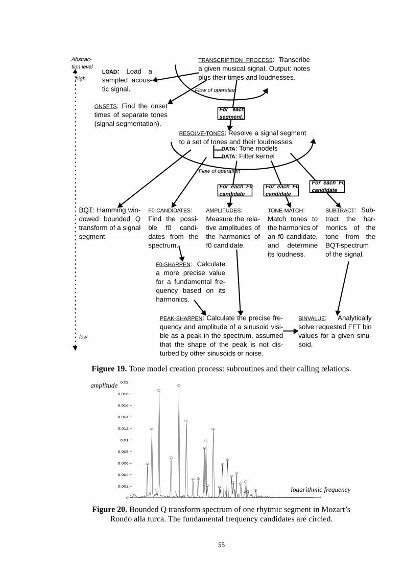
AMPLITUDES:Measure the rela-tive amplitudes ofthe harmonics off0 candidate.

Flow of operation

RESOLVE-TONES: Resolve a signal segmentto a set of tones and their loudnesses.

DATA : Filter kernelDATA : Tone models

Flow of operation

low

high

F0-CANDIDATES:Find the possi-ble f0 candi-dates from thespectrum.

Abstrac-tion level

TRANSCRIPTION PROCESS: Transcribea given musical signal. Output: notesplus their times and loudnesses.

TONE-MATCH:Match tones tothe harmonics ofan f0 candidate,and determineits loudness.

SUBTRACT: Sub-tract the har-monics of thetone from theBQT-spectrumof the signal.

BINVALUE: Analyticallysolve requested FFT binvalues for a given sinu-soid.

F0-SHARPEN: Calculatea more precise valuefor a fundamental fre-quency based on itsharmonics.

ONSETS: Find the onsettimes of separate tones(signal segmentation).

BQT: Hamming win-dowed bounded Qtransform of a signalsegment.

LOAD: Load asampled acous-tic signal.

For each F0candidate

For each F0candidate

For each F0candidate

Figure 19.Tone model creation process: subroutines and their calling relations.

For eachsegment.

PEAK-SHARPEN: Calculate the precise fre-quency and amplitude of a sinusoid visi-ble as a peak in the spectrum, assumedthat the shape of the peak is not dis-turbed by other sinusoids or noise.

amplitude

0 50 100 150 200 250 300 350 400 4500

0.002

0.004

0.006

0.008

0.01

0.012

0.014

0.016

0.018

0.02

Figure 20.Bounded Q transform spectrum of one rhytmic segment in Mozart’sRondo alla turca. The fundamental frequency candidates are circled.

logarithmic frequency

55

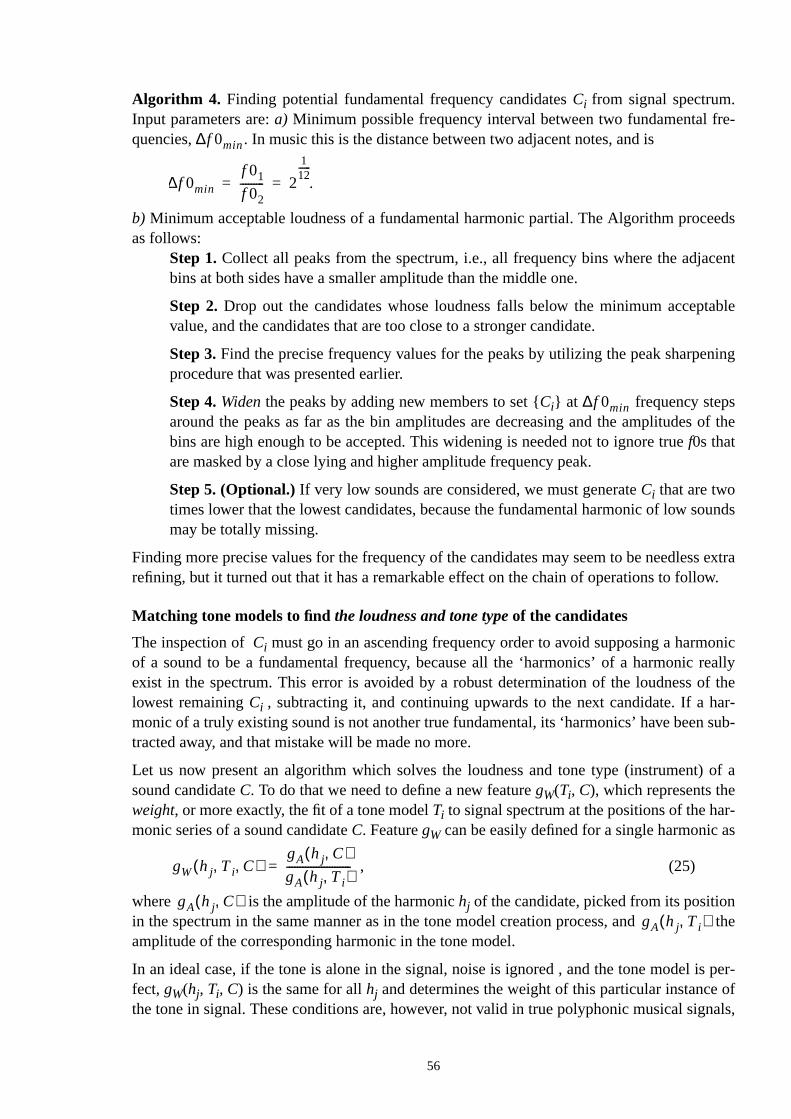
re-

eeds

cent

table

ning

of the

ounds

s extraow.

onicreallyf thear-sub-

) of a

r-as

the

s per-ofnals,

Algorithm 4. Finding potential fundamental frequency candidatesCi from signal spectrum.Input parameters are:a) Minimum possible frequency interval between two fundamental fquencies, . In music this is the distance between two adjacent notes, and is

.

b) Minimum acceptable loudness of a fundamental harmonic partial. The Algorithm procas follows:

Step 1.Collect all peaks from the spectrum, i.e., all frequency bins where the adjabins at both sides have a smaller amplitude than the middle one.

Step 2.Drop out the candidates whose loudness falls below the minimum accepvalue, and the candidates that are too close to a stronger candidate.

Step 3.Find the precise frequency values for the peaks by utilizing the peak sharpeprocedure that was presented earlier.

Step 4.Widenthe peaks by adding new members to set {Ci} at frequency stepsaround the peaks as far as the bin amplitudes are decreasing and the amplitudesbins are high enough to be accepted. This widening is needed not to ignore truef0s thatare masked by a close lying and higher amplitude frequency peak.

Step 5. (Optional.)If very low sounds are considered, we must generateCi that are twotimes lower that the lowest candidates, because the fundamental harmonic of low smay be totally missing.

Finding more precise values for the frequency of the candidates may seem to be needlesrefining, but it turned out that it has a remarkable effect on the chain of operations to foll

Matching tone models to findthe loudness and tone type of the candidates

The inspection ofCi must go in an ascending frequency order to avoid supposing a harmof a sound to be a fundamental frequency, because all the ‘harmonics’ of a harmonicexist in the spectrum. This error is avoided by a robust determination of the loudness olowest remainingCi , subtracting it, and continuing upwards to the next candidate. If a hmonic of a truly existing sound is not another true fundamental, its ‘harmonics’ have beentracted away, and that mistake will be made no more.

Let us now present an algorithm which solves the loudness and tone type (instrumentsound candidateC. To do that we need to define a new featuregW(Ti, C), which represents theweight, or more exactly, the fit of a tone modelTi to signal spectrum at the positions of the hamonic series of a sound candidateC. FeaturegW can be easily defined for a single harmonic

, (25)

where is the amplitude of the harmonichj of the candidate, picked from its positionin the spectrum in the same manner as in the tone model creation process, andamplitude of the corresponding harmonic in the tone model.

In an ideal case, if the tone is alone in the signal, noise is ignored , and the tone model ifect,gW(hj, Ti, C) is the same for allhj and determines the weight of this particular instancethe tone in signal. These conditions are, however, not valid in true polyphonic musical sig

∆f 0min

∆f 0min

f 01

f 02--------- 2

112------

= =

∆f 0min

gW hj Ti C, ,( )gA hj C,( )gA hj Ti,( )------------------------=

gA hj C,( )gA hj Ti,( )

56

,

theres

sses

can

inge mod-

can-

s

udness

nd the

ofneed a

especially because interfering sounds overlap subsets of everymth harmonics of the candidateas discussed earlier. Thus we need to calculate the weight of a whole tone modelTi incandidateC as

, (26)

wherev(•) is the filter that was designed in the previous chapter, and {gW(hj, Ti, C)} is the setof weights of the harmonics of this tone. This value is trustworthy, because we know thatis no sound in a straight harmonic relationbelow the current candidate, or if there is, it habeen subtracted already. On the other hand, only a partly disturbed set {gW(•)} is handled bythe properties of the filterv.

The loudnessof a tone model with unity match can be determined by summing the loudneof its harmonics, calculated by substituting their frequencies and amplitudes tonormal equal-loudness level contours[ISO87]. A rough reference value for the loudness of a tone modelalso be calculated as

, (27)

wherea is a constant,gF(•) means frequency,gA(•) amplitude. This rule-of-thumb works quitewell if the harmonicshj of the tone are in the frequency range 20...2000 Hz. However, usnormal equal-loudness level contours is highly recommended. The loudnesses of the tonels need to be calculated only once, since the loudness of a candidate soundCi can be calcu-lated by finding the best matching tone modelTbest for it, and scaling the loudness ofTbestaccording to its fitgF(Tbest, Ci) to Ci. Thus the loudness of a candidateCi can be written as

. (28)

The above discussion is rewritten in a form of an algorithm.

Algorithm 5. Finding the tone type (instrument) and loudness of a fundamental frequencydidateC.

Step 1.For each instrument, find the tone modelTi, whose fundamental frequency iclosest to the fundamental frequency ofC.

Step 2.Match tone models toC by calculating their fitsgW(Ti,C) to C.

Step 3.Calculate the loudnesses ofC for the differentTi by substituting their fits andunity loudnesses to Equation 28.

Step 4.Choose the instrument, which gives maximum loudness toC, and thus indicatesto be the best matched instrument. Choose the corresponding loudness to be the loof C.

The fundamental frequency of the candidate is already known, and thus we have also fouother parameters of the candidate.

Subtraction procedure

In music it quite often happens that two notes are in a

(29)

relation to each other, andn is an integer number. A method to make correct observationsthe lower sound were earlier presented, but to detect and observe the higher sound we

gW Ti C,( ) v gW hj Ti C, ,( ){ }=

gL T( ) a gF hj T,( ) gA hj T,( )⋅∑⋅=

gL Ci( ) a gW Tbest Ci,( ) gL Tbest( )⋅ ⋅=

f 0lower1n--- f 0higher⋅=

57

was

thetrum.ing

l.

y

rm,

ides

the

-

nce of

or not.Con-

, evend one.

method to lay it bare from under the lower sound which totally overlaps it. This methodpresented earlier, too, and was named subtraction principle.

The features of concern in our transcription program are weightgW(Ti, C) and loudnessgL(C),which are both based on theamplitudesof the harmonics. Thus the very way to compensateeffect of the lower sound is to subtract the amplitudes of its harmonics from the specThere is no trivial way of subtracting a known sinusoid from spectrum. Instead, the followprocedure must be gone through.

Algorithm 6. Subtracting harmonic partials of a soundC from a spectrum, when its tonemodelTi and weight of the modelgW(Ti,C) are known.

Step 1.Initialize j to 1.

Step 2.Calculate the frequencygF(hj) of harmonic j by

and the amplitudegA(hj) of harmonic j by

where is the amplitude of the corresponding harmonic in the tone mode

Step 3.Form a set of spectrum frequency bins {bk}, that are close enough to frequencgF(hj) so that their amplitude value has been changed by the harmonichj. The size of theset {bk} depends on the windowing function that was used in the frequency transfosince the windowing crucially affects how far the shape of a pure sinusoidhj blurs in thespectrum. For a Hamming window it is enought to include two or three bins at both sof the frequencygF(hj).

Step 4.Analytically solve the frequency transform {Hi} of the harmonichj to the spec-trum bins {bj} using the procedure that was presented earlier in this chapter. This isamount of amplitude that the harmonic partialhj has brought to these bins.

Step 5.Subtract from the corresponding bins {bi} to remove the sinusoid fromthe spectrum. The value of the constanta is discussed right after describing this algorithm.

Step 6.If j is smaller than the highest audible harmonic ofC, addj by one and return tostep 2.

What is the right value for the constanta? When we sum two sinusoids having amplitudesA1andA2 and the same frequency, the amplitude of their sum depends on the phase differethe two sinusoids, being between zero and (A1+A2). Value 1 fora is motivated by the fact thatwe cannot know if we have other sinusoids under the ones that are being subtracted,Still we must be sure to totally remove the harmonics that are not overlapping anything.sider a soundC which is alone in the signal. If we subtract usinga value 0.64, for example, thenext candidate (the second harmonic ofC) will receive a large fraction of the energy ofC, andwill erroneously be taken as an independent sound. It is thus safer to subtract enoughthough it reduces the amplitude of the sounds that are totally overlapped by the subtracteFor other sounds it is not fatal to slightly corrupt the values of everykth harmonic (k>1),because of the properties of filterv.

gF hj( ) j gF C( )⋅=

gA hj( ) gW Ti C,( ) gA hj Ti,( )⋅=

gA hj Ti,( )

a Hi{ }⋅

58

loud-ss of thethresh-

loudershold.

ough,ettingalgo-

-downcom-

cho-n the

re intrike

-he dif-

of its

ound.ion in

ings

oise-d the

vide akindshird,

his isile testallow

ayed

Segregation between true and prune sound candidates

Selection of the truly existing sounds from among the candidates is based purely on theirnesses. To adapt to the overall signal level, the loudnesses are scaled so that the loudnemost prominent sound is unity. Candidates whose relative loudnesses are over a certainold are then accepted as true sounds. This is an extremely simple model of themaskingphe-nomena of the human ear: sounds with too low a relative loudness are masked by thesounds, and are not heard. The relative loudness 0.2 is a good starting point for the thre

This loudness-based segregation is straightforward and simple, but works quite well, thas can be seen from the simulation results. We consider spending too much time on sthresholds a waste of time, because the very basis of the calculations is in the precedingrithms, which should give clear prominence to the right sounds.To design a substantially bet-ter decision procedure we should apply so-called top-down knowledge sources, for examplemusical rules that determine the notes that are likely to play together or in sequence. Topprocessing will be discussed in Chapter 8. In the current system it is not used, but all notebinations and sequences are assumed equally probable.

7.6 Simulations

All the simulations were made using one instrument, piano. A percussive instrument wassen to make rhythm tracking easier, while we do not want to focus the efforts on that. Oother hand, a piano sound is irregular enough to be a ‘real world’ example:

1. Beginning transient contains noisy components. Further, the sinusoid partials aslightly inharmonic relations during the beginning tens of milliseconds, due to the sof a hammer at strings.

2. Shape of the body of a piano produces severalformants: frequency bands where harmonic partials are louder and decay slower because of the resonance of the body. Tferent decay slopes also cause the sound colour to change gradually in the courseplaying.

3. The higher keys have several strings for each note to produce a loud enough sBecause the strings cannot be exactly equally tuned, they cause long term fluctuatthe amplitude envelope of the tone.

4. Cross-resonance. Playing just one note on the keyboard makes also the other free strto start gently resonate along with the hammered string.

Two pianos were used. Initial simulations were made by sampling an electric piano in a nfree environment. In the final simulations we used an acoustic upright piano (Yamaha) anrecording setup that was described in Section 4.3.

Three types of recordings were made. First, the keys were recorded one-by-one to protraining set to the tone model creation process. Second, difficult note mixtures of severalwere recorded to review the performance of the algorithm in possible stumbling points. Tchosen musical pieces were recorded to test practical transcription efficiency.

All recordings were made only once and after that the recording setup was dismounted. Tboth an advantage and a drawback. On one hand it makes the simulations reliable, whmaterial cannot be further adjusted to yield good results. On the other hand, this does notlater reviewing of points where we suspect that the pianist may have unintentionally plsome notes extremely quietly when recording rich note mixtures.

59

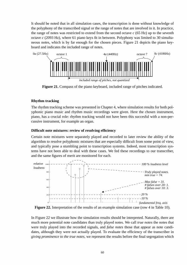
ge ofctice,

lta-o key-

h pol-ment,-per-

f theiew,

sys-scriber,

e are

i-er inich

0).

It should be noted that in all simulation cases, the transcription is done without knowledthe polyphony of the transcribed signal or the range of notes that are involved in it. In prathe range of notes was restricted to extend from the second octavec (65 Hz) up to the seventhoctavec (2093 Hz), where 61 piano keys fit in between. Polyphony was limited to 30 simuneous notes, which is by far enough for the chosen pieces. Figure 21 depicts the pianboard and indicates the included range of notes.

Rhythm tracking

The rhythm tracking scheme was presented in Chapter 4, where simulation results for botyphonic piano music and rhythm music recordings were given. Here the chosen instrupiano, has a crucial role: rhythm tracking would not have been this succesful with a noncussive instrument, for example an organ.

Difficult note mixtures: review of resolving efficiency

Certain note mixtures were separately played and recorded to later review the ability oalgorithm to resolve polyphonic mixtures that are especially difficult from some point of vand typically pose a stumbling point to transcription systems. Indeed, most transcriptiontems have not been able to deal with these cases. We fed these recordings to our tranand the same figures of merit are monitored for each.

In Figure 22 we illustrate how the simulation results should be interpreted. Naturally, thermuch more potential note candidates than truly played notes. We calltrue notesthe notes thatwere truly played into the recorded signals, andfalse notesthose that appear as note canddates, although they were not actually played. To evaluate the efficiency of the transcribgiving prominence to the true notes,we represent the results before the final segregation wh

Figure 21.Compass of the piano keyboard, included range of pitches indicated.

octave1 octave74a (440Hz)0a (27.5Hz) 8c (4186Hz)

included range of pitches, not quantized

relativeloudness

4 4.5 5 5.5 6 6.5 7 7.5

0

20

40

60

80

100

Figure 22.Interpretation of the results of an example simulation case (row 4 in Table 1fundamental freq. axis

10 %

Truly played notes.min true = 74.

Max false = 31.# falses over 20: 1.# falses over 10: 3.

100 % loudness level

20 %

60

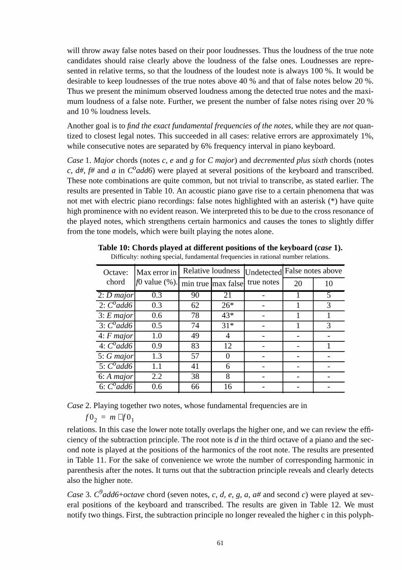
e noterepre-

uld be20 %.

e maxi-20 %

ly 1%,

ed.r. Theat wasuitence ofdiffer

e effi--

sentednic inetects

mustyph-

will throw away false notes based on their poor loudnesses. Thus the loudness of the trucandidates should raise clearly above the loudness of the false ones. Loudnesses aresented in relative terms, so that the loudness of the loudest note is always 100 %. It wodesirable to keep loudnesses of the true notes above 40 % and that of false notes belowThus we present the minimum observed loudness among the detected true notes and thmum loudness of a false note. Further, we present the number of false notes rising overand 10 % loudness levels.

Another goal is tofind the exact fundamental frequencies of the notes, while they arenotquan-tized to closest legal notes. This succeeded in all cases: relative errors are approximatewhile consecutive notes are separated by 6% frequency interval in piano keyboard.

Case1. Major chords (notesc, eandg for C major) anddecremented plus sixthchords (notesc, d#, f#anda in Coadd6) were played at several positions of the keyboard and transcribThese note combinations are quite common, but not trivial to transcribe, as stated earlieresults are presented in Table 10. An acoustic piano gave rise to a certain phenomena thnot met with electric piano recordings: false notes highlighted with an asterisk (*) have qhigh prominence with no evident reason. We interpreted this to be due to the cross resonathe played notes, which strengthens certain harmonics and causes the tones to slightlyfrom the tone models, which were built playing the notes alone.

Case 2. Playing together two notes, whose fundamental frequencies are in

relations. In this case the lower note totally overlaps the higher one, and we can review thciency of the subtraction principle. The root note isd in the third octave of a piano and the second note is played at the positions of the harmonics of the root note. The results are prein Table 11. For the sake of convenience we wrote the number of corresponding harmoparenthesis after the notes. It turns out that the subtraction principle reveals and clearly dalso the higher note.

Case3. C9add6+octavechord (seven notes,c, d, e, g, a, a#and secondc) were played at sev-eral positions of the keyboard and transcribed. The results are given in Table 12. Wenotify two things. First, the subtraction principle no longer revealed the higher c in this pol

Table 10: Chords played at different positions of the keyboard (case 1).Difficulty: nothing special, fundamental frequencies in rational number relations.

Octave:chord

Max error inf0 value (%).

Relative loudnessUndetectedtrue notes

False notes above

min true max false 20 10

2: D major 0.3 90 21 - 1 52: Coadd6 0.3 62 26* - 1 33: E major 0.6 78 43* - 1 13: Coadd6 0.5 74 31* - 1 34: F major 1.0 49 4 - - -4: Coadd6 0.9 83 12 - - 15: G major 1.3 57 0 - - -5: Coadd6 1.1 41 6 - - -6: A major 2.2 38 8 - - -6: Coadd6 0.6 66 16 - - -

f 02 m f01⋅=

61

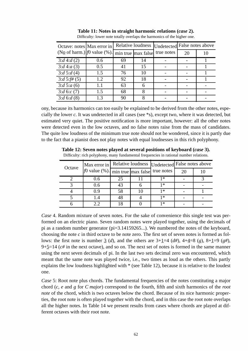
, espe-, butotesidates.

y due.

s per-als of

board,fol-

annerwhichpartly

udest

major

per-erlapsat dif-

ony, because its harmonics can too easily be explained to be derived from the other notescially the lowerc. It was undetected in all cases (see *s), except two, where it was detectedestimated very quiet. The positive notification is more important, however: all the other nwere detected even in the low octaves, and no false notes raise from the mass of candThe quite low loudness of the minimum true note should not be wondered, since it is partlto the fact that a pianist does not play notes with equal loudnesses in this rich polyphony

Case4. Random mixture of seven notes. For the sake of convenience this single test waformed on an electric piano. Seven random notes were played together, using the decimpi as a random number generator (pi=3.14159265...). We numbered the notes of the keychoosing the notec in third octave to be note zero. The first set of seven notes is formed aslows: the first note is number3 (d), and the others are 3+1=4 (d#), 4+4=8 (g), 8+1=9 (g#),9+5=14 (c# in the next octave), and so on. The next set of notes is formed in the same musing the next seven decimals of pi. In the last two sets decimal zero was encountered,meant that the same note was played twice, i.e., two times as loud as the others. Thisexplains the low loudness highlighted with * (see Table 12), because it is relative to the loone.

Case5: Root note plus chords. The fundamental frequencies of the notes constituting achord (c, eandg for C major) correspond to the fourth, fifth and sixth harmonics of therootnoteof the chord, which is two octaves below the chord. Because of its nice harmonic proties, the root note is often played together with the chord, and in this case the root note ovall the higher notes. In Table 14 we present results from cases where chords are playedferent octaves with their root note.

Table 11: Notes in straight harmonic relations (case 2).Difficulty: lower note totally overlaps the harmonics of the higher one.

Octave: notes(No of harm.)

Max error inf0 value (%).

Relative loudnessUndetectedtrue notes

False notes above

min true max false 20 10

3:d 4:d (2) 0.6 69 14 - - 13:d 4:a (3) 0.5 41 15 - - 13:d 5:d (4) 1.5 76 10 - - 13:d 5:f# (5) 1.2 92 18 - - 13:d 5:a (6) 1.1 63 6 - - -3:d 6:c (7) 1.5 68 8 - - -3:d 6:d (8) 1.3 90 8 - - -

Table 12: Seven notes played at several positions of keyboard (case 3).Difficulty: rich polyphony, many fundamental frequencies in rational number relations.

OctaveMax error inf0 value (%).

Relative loudnessUndetectedtrue notes

False notes above

min true max false 20 10

2 0.6 25 11 1* - 33 0.6 43 6 1* - -4 0.9 58 10 1* - 15 1.4 48 4 1* - -6 2.2 18 0 1* - -

62

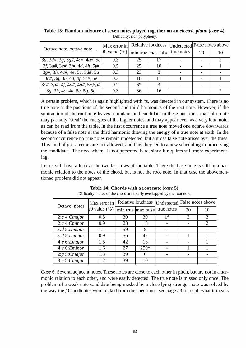
is noif thee notenote,wards

In thee trues.ssingriment-

har-men-

a har-e. Theed byeans

A certain problem, which is again highlighted with *s, was detected in our system. Theretrue note at the positions of the second and third harmonics of the root note. However,subtraction of the root note leaves a fundamental candidate to these positions, that falsmay partially ‘steal’ the energies of the higher notes, and may appear even as a very loudas can be read from the table. In the first occurrence a true note moved one octave downbecause of a false note at the third harmonic thieving the energy of a true note at sixth.second occurrence no true notes remain undetected, but a gross false note arises over thThis kind of gross errors are not allowed, and thus they led to a new scheduling in procethe candidates. The new scheme is not presented here, since it requires still more expeing.

Let us still have a look at the two last rows of the table. There the base note is still in amonic relation to the notes of the chord, but is not the root note. In that case the abovetioned problem did not appear.

Case6. Several adjacent notes. These notes are close to each other in pitch, but are not inmonic relation to each other, and were easily detected. The true note is missed only oncproblem of a weak note candidate being masked by a close lying stronger note was solvthe way thef0 candidates were picked from the spectrum - see page 53 to recall what it m

Table 13: Random mixture of seven notes played together on anelectric piano (case 4).Difficulty: rich polyphony.

Octave note, octave note, ...Max error inf0 value (%).

Relative loudnessUndetectedtrue notes

False notes above

min true max false 20 10

3d, 3d#,3g, 3g#,4c#,4a#,5c 0.3 25 17 - - 23f, 3a#,3c#,3f#, 4d, 4h, 5f# 0.5 25 10 - - 13g#,3h, 4c#,4e,5c, 5d#,5a 0.3 23 8 - - -3c#,3g, 3h, 4d, 4f, 5c#,5e 0.2 10 11 1 - 1

3c#,3g#, 4f, 4a#, 4a#,5c,5g# 0.2 6* 3 - - -3g, 3h, 4c, 4a, 5e, 5g, 5g 0.3 36 16 - - 2

Table 14: Chords with a root note (case 5).Difficulty: notes of the chord are totally overlapped by the root note.

Octave: notesMax error inf0 value (%).

Relative loudnessUndetectedtrue notes

False notes above

min true max false 20 10

2:c 4:Cmajor 0.5 30 30 1* 2 22:c 4:Cminor 0.9 23 18 - - 23:d 5:Dmajor 1.1 59 8 - - -3:d 5:Dminor 0.9 56 42 - 1 14:e6:Emajor 1.5 42 13 - - 14:e6:Eminor 1.6 27 250* - 1 12:g 5:Cmajor 1.3 39 6 - - -3:e5:Cmajor 1.2 39 10 - - -

63

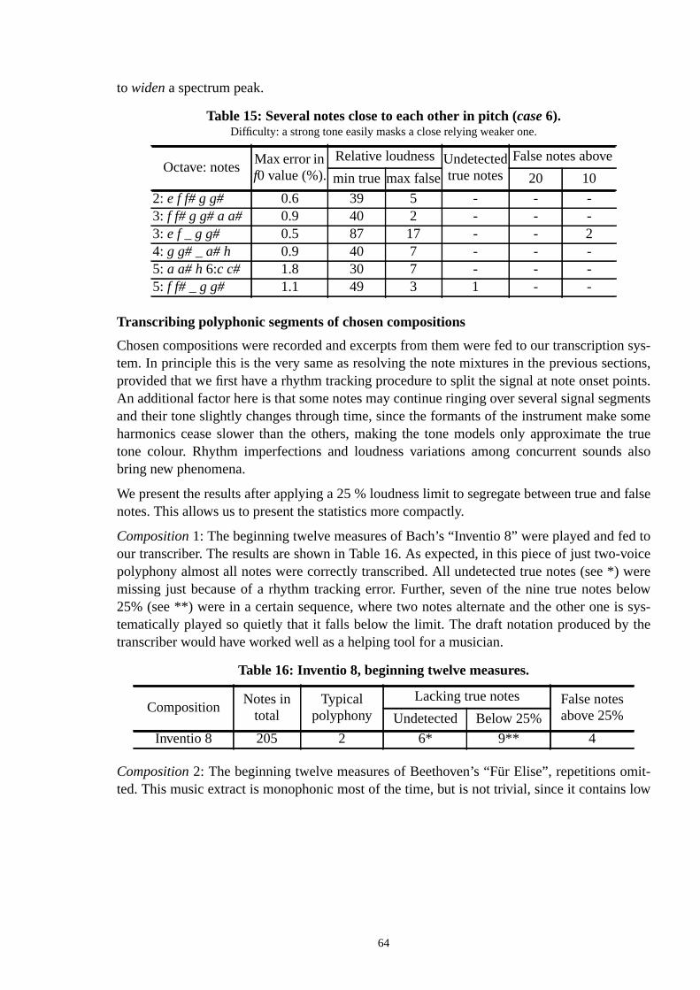
n sys-tions,oints.mentssomee true

s also

d false

d tovoicewere

belowis sys-the

it-low

to widen a spectrum peak.

Transcribing polyphonic segments of chosen compositions

Chosen compositions were recorded and excerpts from them were fed to our transcriptiotem. In principle this is the very same as resolving the note mixtures in the previous secprovided that we first have a rhythm tracking procedure to split the signal at note onset pAn additional factor here is that some notes may continue ringing over several signal segand their tone slightly changes through time, since the formants of the instrument makeharmonics cease slower than the others, making the tone models only approximate thtone colour. Rhythm imperfections and loudness variations among concurrent soundbring new phenomena.

We present the results after applying a 25 % loudness limit to segregate between true annotes. This allows us to present the statistics more compactly.

Composition1: The beginning twelve measures of Bach’s “Inventio 8” were played and feour transcriber. The results are shown in Table 16. As expected, in this piece of just two-polyphony almost all notes were correctly transcribed. All undetected true notes (see *)missing just because of a rhythm tracking error. Further, seven of the nine true notes25% (see **) were in a certain sequence, where two notes alternate and the other onetematically played so quietly that it falls below the limit. The draft notation produced bytranscriber would have worked well as a helping tool for a musician.

Composition2: The beginning twelve measures of Beethoven’s “Für Elise”, repetitions omted. This music extract is monophonic most of the time, but is not trivial, since it contains

Table 15: Several notes close to each other in pitch (case 6).Difficulty: a strong tone easily masks a close relying weaker one.

Octave: notesMax error inf0 value (%).

Relative loudnessUndetectedtrue notes

False notes above

min true max false 20 10

2: e f f# g g# 0.6 39 5 - - -3: f f# g g# a a# 0.9 40 2 - - -3: e f _ g g# 0.5 87 17 - - 24: g g# _ a# h 0.9 40 7 - - -5: a a# h6:c c# 1.8 30 7 - - -5: f f# _ g g# 1.1 49 3 1 - -

Table 16: Inventio 8, beginning twelve measures.

CompositionNotes in

totalTypical

polyphonyLacking true notes False notes

above 25%Undetected Below 25%

Inventio 8 205 2 6* 9** 4

64

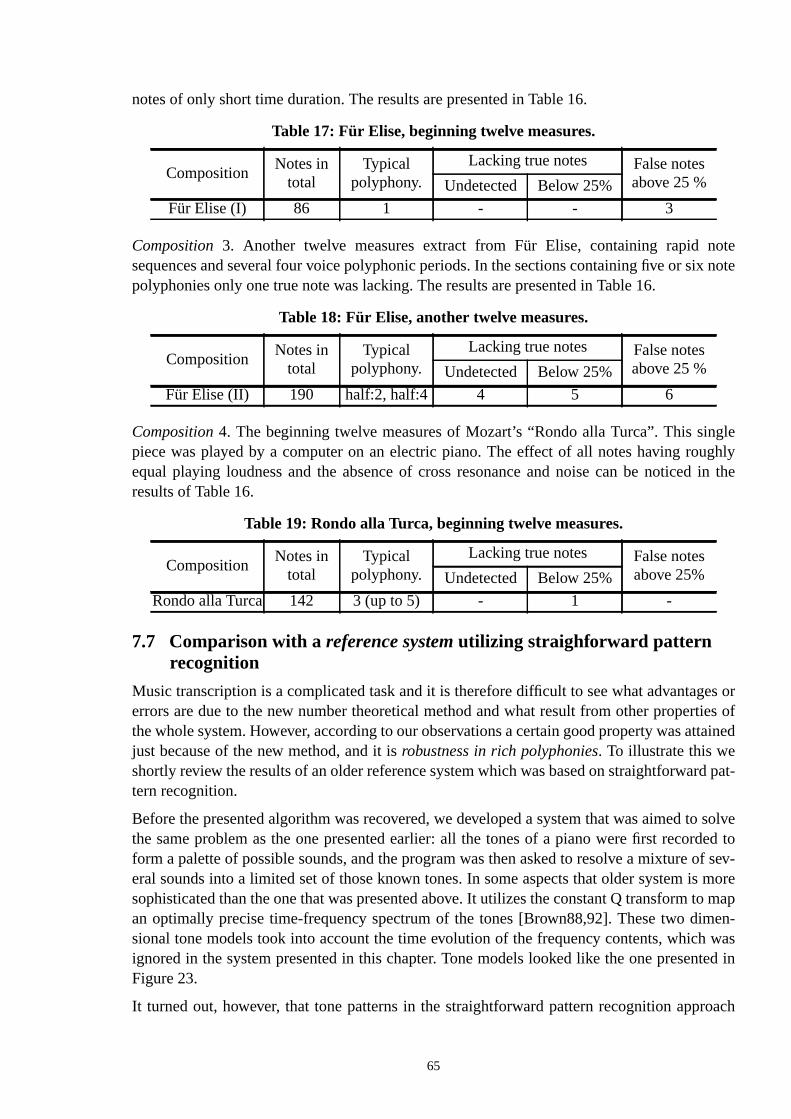
otex note

gleughlyd in the

es orties oftained

d pat-

o solveded toof sev-s moreto mapmen-

wasted in

roach

notes of only short time duration. The results are presented in Table 16.

Composition3. Another twelve measures extract from Für Elise, containing rapid nsequences and several four voice polyphonic periods. In the sections containing five or sipolyphonies only one true note was lacking. The results are presented in Table 16.

Composition4. The beginning twelve measures of Mozart’s “Rondo alla Turca”. This sinpiece was played by a computer on an electric piano. The effect of all notes having roequal playing loudness and the absence of cross resonance and noise can be noticeresults of Table 16.

7.7 Comparison with areference system utilizing straighforward patternrecognition

Music transcription is a complicated task and it is therefore difficult to see what advantagerrors are due to the new number theoretical method and what result from other properthe whole system. However, according to our observations a certain good property was atjust because of the new method, and it isrobustness in rich polyphonies. To illustrate this weshortly review the results of an older reference system which was based on straightforwartern recognition.

Before the presented algorithm was recovered, we developed a system that was aimed tthe same problem as the one presented earlier: all the tones of a piano were first recorform a palette of possible sounds, and the program was then asked to resolve a mixtureeral sounds into a limited set of those known tones. In some aspects that older system isophisticated than the one that was presented above. It utilizes the constant Q transforman optimally precise time-frequency spectrum of the tones [Brown88,92]. These two disional tone models took into account the time evolution of the frequency contents, whichignored in the system presented in this chapter. Tone models looked like the one presenFigure 23.

It turned out, however, that tone patterns in the straightforward pattern recognition app

Table 17: Für Elise, beginning twelve measures.

CompositionNotes in

totalTypical

polyphony.Lacking true notes False notes

above 25 %Undetected Below 25%

Für Elise (I) 86 1 - - 3

Table 18: Für Elise, another twelve measures.

CompositionNotes in

totalTypical

polyphony.Lacking true notes False notes

above 25 %Undetected Below 25%

Für Elise (II) 190 half:2, half:4 4 5 6

Table 19: Rondo alla Turca, beginning twelve measures.

CompositionNotes in

totalTypical

polyphony.Lacking true notes False notes

above 25%Undetected Below 25%

Rondo alla Turca 142 3 (up to 5) - 1 -

65

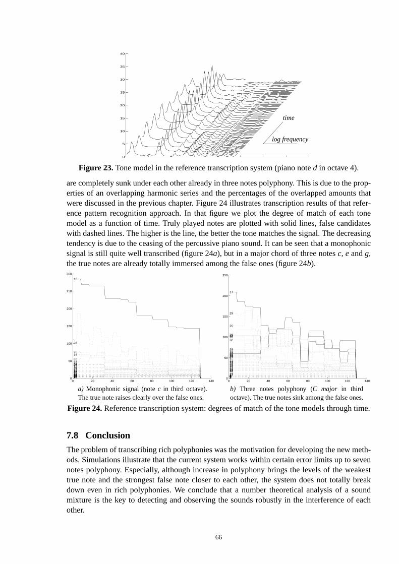
prop-ts thatrefer-tone

ateseasingphonic

eth-evenakestbreak

oundeach

time.

are completely sunk under each other already in three notes polyphony. This is due to theerties of an overlapping harmonic series and the percentages of the overlapped amounwere discussed in the previous chapter. Figure 24 illustrates transcription results of thatence pattern recognition approach. In that figure we plot the degree of match of eachmodel as a function of time. Truly played notes are plotted with solid lines, false candidwith dashed lines. The higher is the line, the better the tone matches the signal. The decrtendency is due to the ceasing of the percussive piano sound. It can be seen that a monosignal is still quite well transcribed (figure 24a), but in a major chord of three notesc, eandg,the true notes are already totally immersed among the false ones (figure 24b).

7.8 Conclusion

The problem of transcribing rich polyphonies was the motivation for developing the new mods. Simulations illustrate that the current system works within certain error limits up to snotes polyphony. Especially, although increase in polyphony brings the levels of the wetrue note and the strongest false note closer to each other, the system does not totallydown even in rich polyphonies. We conclude that a number theoretical analysis of a smixture is the key to detecting and observing the sounds robustly in the interference ofother.

0 20 40 60 80 100 120 140 1600

5

10

15

20

25

30

35

40

Figure 23.Tone model in the reference transcription system (piano noted in octave 4).

time

log frequency

0 20 40 60 80 100 120 1400

50

100

150

200

250

300

1234567891011

12

13

14

15

161718

1920212223

24

25

26

2728

2930

31

3233343536

0 20 40 60 80 100 120 1400

50

100

150

200

250

123456789101112

13

14

15

16

17

18

19

20

21222324

25

26

27

28

29

30

31

32

3334

35

36

a) Monophonic signal (notec in third octave).The true note raises clearly over the false ones.

b) Three notes polyphony (C major in thirdoctave). The true notes sink among the false ones.

Figure 24.Reference transcription system: degrees of match of the tone models through

66

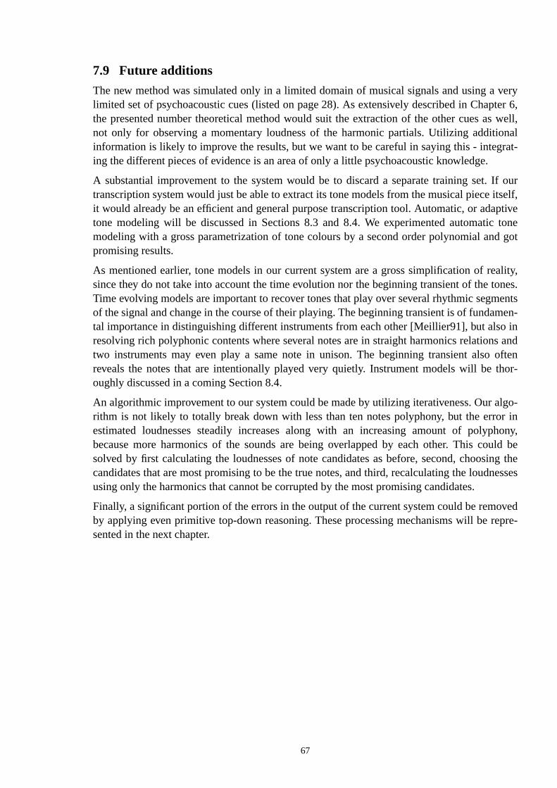
veryter 6,well,

onalrat-

If ouritself,ptivetone

d got

ality,ones.

entsmen-o ins andoften

thor-

lgo-r inhony,uld being thenesses

ovedepre-

7.9 Future additions

The new method was simulated only in a limited domain of musical signals and using alimited set of psychoacoustic cues (listed on page 28). As extensively described in Chapthe presented number theoretical method would suit the extraction of the other cues asnot only for observing a momentary loudness of the harmonic partials. Utilizing additiinformation is likely to improve the results, but we want to be careful in saying this - integing the different pieces of evidence is an area of only a little psychoacoustic knowledge.

A substantial improvement to the system would be to discard a separate training set.transcription system would just be able to extract its tone models from the musical pieceit would already be an efficient and general purpose transcription tool. Automatic, or adatone modeling will be discussed in Sections 8.3 and 8.4. We experimented automaticmodeling with a gross parametrization of tone colours by a second order polynomial anpromising results.

As mentioned earlier, tone models in our current system are a gross simplification of resince they do not take into account the time evolution nor the beginning transient of the tTime evolving models are important to recover tones that play over several rhythmic segmof the signal and change in the course of their playing. The beginning transient is of fundatal importance in distinguishing different instruments from each other [Meillier91], but alsresolving rich polyphonic contents where several notes are in straight harmonics relationtwo instruments may even play a same note in unison. The beginning transient alsoreveals the notes that are intentionally played very quietly. Instrument models will beoughly discussed in a coming Section 8.4.

An algorithmic improvement to our system could be made by utilizing iterativeness. Our arithm is not likely to totally break down with less than ten notes polyphony, but the erroestimated loudnesses steadily increases along with an increasing amount of polypbecause more harmonics of the sounds are being overlapped by each other. This cosolved by first calculating the loudnesses of note candidates as before, second, chooscandidates that are most promising to be the true notes, and third, recalculating the loudusing only the harmonics that cannot be corrupted by the most promising candidates.

Finally, a significant portion of the errors in the output of the current system could be remby applying even primitive top-down reasoning. These processing mechanisms will be rsented in the next chapter.

67

m-upm-up:itoryis also

prioration

use auble-f an

om-uptemmod-e was

g isplacep

have

on isroc-

implyays.

be dis-

t someources‘lin-

te howitec-

8 Top-Down Processing

Until now, our discussion on music transcription has almost exclusively concerned bottoprocessing techniques. They are characterized by the fact that all information flows bottoinformation is observed in an acoustic waveform, combined to provide meaningful audcues, and passed to higher level processes for further interpretation. This approachcalleddata-driven processing.

Top-down processing utilizes internal, high-level models of the acoustic environment andknowledge of the properties and dependencies of the objects in it. In this approach informalso flows top-down: a sensing system collects evidence that would either justify or cachange in an internal world model and in the state of the objects in it. This approach is docalledprediction-drivenprocessing, because it is strongly dependent on the predictions oabstracted internal model, and on prior knowledge of the sound sources [Ellis96].

The science of perception and the perceptual models of audition are dominated by a bottapproach, most often ignoring top-down flow of information in the human auditory sys[Slaney95]. In our transcription system, the only top-down mechanism is its use of toneels, i.e., prior knowledge of the instrument sounds. On the other hand, musical knowledgtotally ignored, assuming all note combinations and sequences equally probable.

The foundation of signal analysis is still in reliable low-level observations. Without being ableto reliably extract information at the lowest level, no amount of higher level processingoing to resolve a musical signal. It is therefore clear that top-down processing cannot rethe functions of a bottom-up analysis. Instead,top-down techniques can add to bottom-uprocessing and help it to solve otherwise ambiguous situations. Top-down rules may confirman interpretation or cancel out some others. On the other hand, high-level knowledge canguidethe attention and sensitivity of the low-level analysis.

It should be noted that top-down processing does not require that the information shouldoriginatedat a high-level process. Conversely, all top-down processing should be highlyinter-activeand adapt to the signal at hands. For example, context is utilized when informaticollected at a low level, interpreted at a higher level, and brought back to affect low-level pesses. Similarly, internal tone models should originate from low-level observations.

A hierarchy of information representations, as discussed in Chapter 3, does not need tobottom-up processing: representations may be fixed, and still information flows both wData representations, processing algorithms, and an implementation architecture shouldcussed separately, according to the desirable properties of each.

In this chapter we first discuss the shortcomings of pure bottom-up systems and representop-down phenomena in human hearing. Second, we represent top-down knowledge sthat can be used in music transcription: use of context, instrument models, and primitiveguistic’ dependencies of note sequences and combinations in music. Then we investigathat information could be practically used, and finally propose some implementation archtures.

68

facteasonreta-to a

ons ofnd itation

racta-f

akese ofrk

audi-

d theanal-s.

rocess-y forentlyate a

s thepeechburst

lable,

essingch, ind to as, andmis-

ent

in ac linesere

8.1 Shortcomings of pure bottom-up systems

The critique of pure bottom-up models of the human auditory system is not only due to thethat they fail to model some important processes in human perception. The very basic rfor criticism is that often these models are not sufficient to provide a reliable enough interption of acoustic information that comes from an auditory scene. This applies especiallygeneral purpose computational auditory scene analysis, where some top-down predictian internal world model are certainly needed. For example, even a human listener will fidifficult to analyze the number of persons and their actions in a room by acoustic informonly, without prior knowledge of the actual physical setting in that room.

Transcription of musical signals is a substantially more specialized task, and thus more tble for bottom-up systems. Nevertheless,inflexibility, when it comes to the generality osounds and musical styles, is a problem that is largely derived from systems’ inability to moverall observations of the data and let that knowledge flow back top-down for the purpoadapting the low-level signal analysis. Another lacking facet of flexibility is the ability to wowith obscured or partly corrupted data, which would still be easily handled by the humantory system.

In the following sections, we will represent knowledge sources and mechanisms that adintelligence of bottom-up systems. That knowledge can be used to prevent the bottom-upysis being misled in some situations, or to solve otherwise ambiguous mixtures of sound

8.2 Top-down phenomena in hearing

Psychoacoustic experiments have revealed several phenomena that suggest top-down ping to take place in human auditory perception. Although this has been known alreadyears, explicit critique of pure bottom-up perception models has emerged only very rec[Slaney95, Ellis96, Scheirer96]. In this section we review some phenomena that motivtop-down viewpoint to perception.

Auditory restorationrefers to an unconscious mechanism in hearing, which compensateeffect of masking sounds [Bregman90]. In an early experiment, listeners were played a srecording in which a certain syllable had been deleted and replaced by a noise[Warren70]. Because of the linguistic context, the listeners also ‘heard’ the removed syland were even unable to identify exactly where the masking noise burst had occurred.

Slaney describes an experiment of Remez and Rubin which indicates that top-down proctakes place in organizing simultaneous spectral features [Slaney95]. Sine-wave speewhich the acoustic signal was modelled by a small number of sinusoid waves, was playegroup of listeners. Most listeners first recognized that signal as a series of tones, chirpblips with no apparent linguistic meaning. But after some period of time, all listeners untakably heard the words and had difficulties in separating the tones and blips. Thelinguisticinformationchanged the perception of the signal. In music, internal models of the instrumsounds and tonal context have an analogous effect.

Scheirer mentions Thomassen’s observation, which indicates thathigh-level melodic under-standingin music may affect the low-level perception of the attributes of a single soundstream [Scheirer96a]. Thomassen observed that certain frequency contours of melodilead to a percept of anaccentedsound - as it would have been played stronger, although thwas no change in the loudness of the sounds [Thomassen82].

69

endingeners

alsers: toof the

me andk of aed toatten-

low-e

fore inter-monicstill be

sed onnowl-.6.

ticallyssarilyernale fromnownimilartably

ustBysepa-

et of

lodicl andpted

Slaney illustrates theeffect of contextby explaining Ladefoged’s experiment, where the samconstant sample was played after two different introductory sentences [Slaney95]. Depeon the speaker of the introductory sentence “Please say what this word is: -”, the listheard the subsequent constant sample to be either “bit” or “bet” [Ladefoged89].

Memory and hearing interact. In Chapter 6.3 we stated that paying attention to time intervin rhythm and to frequency intervals of concurrent sounds has a certain goal among othunify the sounds to form a coherent structure that is able to express more than anysounds alone. We propose that also thestructurein music has this function: similarities in twosound sequencies tie these bigger entities together, although they may be separated in timay differ from each other in details. These redundancies and repetitions facilitate the tashuman listener, and raise expectations in his mind. Only portions of a common theme nebe explicitly repeated to reconstruct the whole sequence in a listener’s mind, and specialtion can be paid to intentional variations in repeated sequencies.

8.3 Utilization of context

Certain aspects of the human auditory restoration can be quite reliably modelled, if thelevel conditions and functions of that phenomenon can just be determined. These includillu-sory continuityeither in time or in frequency dimension. If a stable sound becomes brokena short time and an explaining event (such as a noise burst) is present, that period can bpolated, since the human auditory system will do the same. On the other hand, if the harpartials of a sound are missing or corrupted at a certain frequency band, the sound canrecovered by finding a harmonic series at adjacent bands.

The auditory restoration example in Section 8.2 represents a type of restoration that is balinguistic knowledge and cannot be done as easily. That requires applying higher level kedge. Primitive ‘linguistic’ dependences in music will be discussed in Sections 8.5 and 8

In Section 5.4 we made a point that separating harmonically related sounds is theoreambiguous without internal models of the component sounds. These models do not neceneed to be pre-defined, but may be found in the context of an ambiguous mixture. Intmodels should be assembled and adapted at moments when that information is laid barunder the interference of other sounds, and used at more complicated points. It is well kthat if two sound sequences move in parallel in music, playing the same notes or two smelodies with a harmonically related frequency separation, the auditory system will ineviconsider them a single unit. Typically this is not the composer’s intention, but music mintroduce theatomic patterns, sounds, by representing them as varying combinations.recovering these atomic sounds, melodic lines of two instruments can be perceptuallyrated from each other, although they would instantaneously totally overlap each other.

Musical signals are redundant at many levels. Not only do they consist of a limited sinstrumental sounds, but they also havestructural redundancy. The ability of a listener to fol-low rich polyphonies can be improved by a thematic repetition, and by adding new melayers or variations one by one. This strategy is often employed, for example, in classicain jazz music, when the richness and originality of climax points could not be directly acceby a listener.

70

ever,thodsnt to

anism,thate metmod-lly inlved

terial.from

ment

rtainge ofusicalaudi-

iecein

on-feredn is tod in

or-lsof anesis.

tst onet mays to active

andof

-

to hearoposers thatrent

8.4 Instrument models

In our transcription system, tone models were the only top-down knowledge source. Howcareful compilation of these models, coupled with the presented number theoretical mecould solve transcription problems that have been earlier impossible. Indeed, we waemphasize that the use of instrument models is a powerful top-down processing mechprovided that this information can be collected. Even more, we showed in Section 5.5these models are indispensable because of the theoretical ambiguity that will otherwise bin separating harmonic mixtures of musical sounds. Separating them without instrumentels is possible only if there are other distinguishing perceptual cues. However, practicaevery single piece of music there will be a multitude of note mixtures that cannot be resowithout instrument models.

This does not mean that instrument models must be built beforehand from a training maThey can be assembled either from separate training material, or during the transcriptionthe musical signal itself, or by combining these two: starting from a set of standard instrumodels that are thenadapted,reconciled using the musical signal. We use the termstonemodelandtimbremodel in different meanings, the former referring to a model of a sound at a cepitch, and the latter to the model of instrument characteristics that apply to its whole ransounds. The term timbre alone means the distinctive character of the sounds of a minstrument, apart from their pitch and intensity, ‘sound colour’. It seems that the humantory system uses timbre models, since it tends to model the source, not single sounds.

If our transcription system were just able to extract its tone models from the musical pitself, it would be an efficient and general purpose transcription tool. A critical problemdoing that is torecognizean instrument, to know what model to use when needed, or to reccile by adapting when it is possible. Controlled adapting by accounting only the non-interpartials would then be possible, based on the analysis in Chapter 6. Another problem thefind a parametrization for the models that allows using the information of just one sounrefining the timbre model of the whole instrument.

Since we think that distinguishing different instruments from each other is of critical imptance, we concentrate on studyingwhat is the information that should be stored in the mode,i.e., what are the types of information that give a distinctive character to the soundsinstrument. Parametrization and use of that information goes beyond the scope of this th

We have taken adimensional approachin organizing and distinguishing timbres of differeninstruments. This means that their relations or similarities cannot be expressed using juattribute, but a timbre can resemble another in different ways, as well as a physical objecresemble another in size, shape, material, or colour. A classic study on organizing timbrefeature space of features was published by Grey in 1977 [Grey77]. Grey found three distindimensions of timbres.1) The brightness of sounds: spectral energy distribution to highlow harmonic partials.2) The amount of spectral fluctuation through time, i.e., the degreesynchronicity in the amplitude envelopes of the partials.3) Presence and strength of high frequency energy during the attack period of the sounds.

We propose a selection of dimensions that pays attention to the fact that a human tendsthesourceof a sound, and understands a sound by imagining its source. Therefore we prthat the fundamental dimensions of a timbre space are properties of sound sources, factoleave an informative ‘fingerprint’ to the sound, and enable a listener to distinguish diffe

71

f Grey,tural,

thway

racts

pectse, wectively

nds ofutioninent

ducesd har-

d fre-ucturegetherothers.e tim-

. Theound actionre then90].

Thisthat

ecay-g isverseual-por-nds.urst

sources, instruments, from each other. These dimensions bear resemblance to those obut the attention is not paid to the signal but to its source, which we consider more nainformative, and descriptive. The ‘fingerprints’ to a sound are set by

1. Properties of the vibrating source.2. Resonance properties of the body of a musical instrument. That is the immediate pa

of the produced sound, intensifying or attenuating certain frequencies.3. Properties of the driving force that sets a sound playing. The mechanism how it inte

with the vibrating source to give birth to a sound.

It is a well known fact that the human auditory system is able to separate the first two asabove [Bregman90]. Since especially the third aspect is usually ignored in the literaturwill discuss it more than the others. It seems that these three properties of the source effeexplain the information that is present in a resulting acoustic signal.

Vibrating source

A vibrating source is the very place where a sound is produced. It causes at least two kispectral features. First, brightness of a sound, which is determined by the energy distribbetween high and low frequency components. Brightness was found to be the most promdistinguishing feature in the experiments of Grey. Second, a vibrating source often procertain regularities in the harmonic series of a sound. In a clarinet sound, for example, odmonics are stronger than the even ones.

Body of a musical instrument

The termformantrefers to any of the several characteristic bands of resonance, intensifiequency bands that together determine the quality of a spoken vowel, for example. The strof the body of a musical instrument causes formants. Its size, shape and material altomake it function as a filter, which intensifies some frequency bands and attenuates someHarmonic partials at formant frequencies play louder and decay slower, which causes thbre of the sound to smoothly change in the course of its playing.

One good way to model the body of an instrument is to determine its frequency responsepattern of intensified and attenuated frequency bands affects the perceived timbre of a slot. Bregman clarifies this by taking different spoken vowels as an example. Their distindepends on the locations of the lowest three formants of the vocal tract. The lowest two amost important and are enough to provide a clear distinction between the vowels [Bregma

Driving force

A musical sound typically consists of an attack transient followed by a steady sound.structure derives itself from the physical production of a sound: the driving phenomenonsets the sound playing leaves its ‘fingerprint’ to the sound before it stabilizes or starts ding. A human listener is able to recognize, for example, the way in which a guitar strinplugged, or to hear out the noisy turbulence of air in the beginning of the sound of a transflute. The transient, in spite of its very short duration, is very important for the perceived qity of the sound [Meillier91]. An analysis of musical instrument sounds shows that a largetion of the spectral information of the sound comes out during the first tens of millisecoThis applies especially to percussive sounds [Meillier91]. The beginning information bmight be utilized as a ‘label’ introducing the sound source.

72

sform,sinceot in

ands meth-r91,are

e sig-ow-lving

halfband

t can

framegth ofin is

hat fre-y binsame

ent of

pactm ofy bins,posed-50),abouttions

nalsation

tical

Measuring the attack transient

Frequency transforms that were discussed in Chapter 3, such as FFT or bounded Q tranare not very suitable for measuring the precise time evolution of frequency components,they are designed to be effective in providing frequency information in one time frame, nobserving the time evolution of certain frequencies, when extremely short time framesanalysis steps must be used. The usefulness of several high-resolution spectral analysiods were evaluated in order to yield precise information of the attack transient [MeillieLaroche93, Kay88]. A crucial drawback of the methods in our simulations was that theycomputationally complex and also sensitive to the choice of analysis parameters and to thnal to which they are applied. This prevented us from their practical utilization. In the folling, we propose a quite straightforward alternative method for extracting precise time evoamplitude envelopes of the frequency components of interest.

The Fourier transformX(k) of a sampled time domain signalx(nT) is calculated as

, (30)

wherek is a discrete frequency bin, zero corresponding to zero frequency, and tothe sampling rate. This transform can be effectively calculated over the whole frequencyin certain time frame using the fast Fourier transform. We pay attention to the fact that ialso be efficiently calculated at successive time frames for a certain frequency bin.

When a certain frequency bin is under inspection, the length of the time domain analysiscan be adjusted to be a multiple of the wavelength of that frequency. In this case the lenthe time frame may be very short (say, three waves), the windowing function in time domanot necessary, and we can extract a precise sample-by-sample amplitude envelope of tquency through time. This is done by first calculating the transform for a certain frequencas usual, and storing all the elements of the sum in Equation 30. Now the transform of thebin in a time frame one sample later can be calculated just by subtracting the first elemthe sum, and adding a new element, which is calculated by

, (31)wheren now points to the sample that is right after the previous frame.

A property of the sinusoid track representation of sound (see Chapter 3) is that it is comand still bears high perceptual fidelity to the original sound. The peaks in the BQT spectruthe beginning of a sound reveal the sinusoids of interest, and therefore also the frequencwhose amplitude envelope should be followed to model that attack of a sound. The prospectral analysis method is efficient, since the number of sinusoids is limited (typically 10and the attack transient over which their amplitude envelope is tracked is very short (50 ms). A more advanced variant of this method could also follow the frequency fluctuaof a sinusoid, but representing its details is not relevant in our scope.

8.5 Sequential dependencies in music

Most speech recognition systems today use linguistic information in interpreting real sigwhere single phonemes may be obscured or too short to be recognized only by the informin a single time frame. Linguistic rules are typically very primitive, such as a table of statis

X k( ) x nT( ) ej– k

2πnTN

--------------⋅ ⋅⋅

n 0=

N 1–

∑=

kN2----=

x nT( ) ej– k

2πnTN

--------------⋅ ⋅⋅

73

. This

en thed thesence.

ouldnoteshas

archers’tran-tostandound

ing toaration

dura-a sec-and isn

l pitchd themposi-

thetion tol roleential

anuencyelo-okenn90].

. Thisusic,on75].

thosea cer-rcep-or a

nitivenotesrhyth-

probabilities for the existence of certain two or three letter sequences in a given languagekind of data can be utilized in ahidden Markov model (HMM), which basically implements astate machine, where single letters are the states, and probabilities for transitions betwestates have been calculated in the language. Based on both low-level observations anhigh-level constraints, a sensing system then determines the most probable letter seque

In [Scheirer96a], Scheirer asks whether primitive ‘linguistic’ dependencies of this kind cbe found for note sequences in music, and under what circumstances following singleand polyphonic lines is possible, difficult or impossible for humans. Fortunately, Bregmanstudied these dependencies and has collected the results of both his own and other resework in [Bregman90]. Since that information has been practically ignored by the musicscription community, we will shortly review it in the following. Bregman’s intention is notenumerate the compositional rules of any certain musical style, but rather to try to underhow the primitive principles of perception are being used in music to make complicated scombination suit human perception.

Sequential coherence of melodies - a review on Bregman’s results

Both time and frequency separations affect the integrity of perceived sequencies, accordBregman’s experiments. These two have such a correlation that as the frequency sepbecomes wider, a note sequence must slow down in order to maintain its coherence. Thetion of a note in Western music typically falls in the decade between one and one tenth ofond, and if a note is shorter that this, it tends to stay close to its neighbors in frequency,used to create what Bregman calls anornamentaleffect. An ornament note is perceived only ia relation to another, and does not itself help to define a melody.

Note sequences can be effectively integrated together by letting them advance by smaltransitions. To illustrate that, Bregman refers to the results of Otto Ortmann, who surveyesizes of the frequency intervals between successive notes in several classical music cotions, totalling 23000 intervals [Ortmann26]. He found that the smallest transitions weremost frequently used, and the number of occurrences dropped roughly in inverse proporthe size of the interval. What is most interesting, harmonic intervals do not play a speciain sequences, but it is only the size of the difference in log frequency that affects sequintegration. Sequential integration by frequency proximity can be illustrated by lettinginstrument play a sequence of notes, where every second note is played at a high freqrange and every other at a low range. This will be inevitably perceived as two distinct mdies: frequency proximity overcomes the temporal order of notes. A melody may be unbrover a large frequency leap only in the case it does not find a better continuation [Bregma

Timbre is an important perceptual cue in grouping sounds to their sources of productionis why timbral similarities can be effectively used for the purpose of grouping sounds in mand for carrying a melody through the sounds of an accompanying orchestration [Ericks

As mentioned earlier, Bregman does not intend to enumerate musical rules that go abovethat can be explained by universal perceptual principles. However, he pays attention totain higher-level sequential principle that seems to be justified by some general rule of petion. That is the fact that a dissonant combination of notes is usually followed by a notemixture of notes which is more stable in the musical system and is able to provide a cogreference point, a ‘melodic anchor’. Furthermore, these inharmonious combinations oftypically do not set on together with other notes, but are placed in between the strongest

74

urrente able

ounds.effec-toerely

isso-entionin

doesc maythoutor theeparate

e tran-ant tog rich

d willmusi-

imericwith

usical

tesch sin-

ted.itches,pro-d by

mmonments,

mic pulses to serve as a short moment of tension between two stabler states.

8.6 Simultaneity dependencies

In Section 6.3 we discussed how music uses harmonic frequency relations to group concnotes together. This takes place for two reasons. First, notes must be knitted together to bto represent higher-level forms that cannot be expressed by single or unrelated atomic sSecond, the spectral components of harmonically related sounds match together, whichtively reduces the complexityof calculations that are needed in the human auditory systemgroup frequency components to acoustic entities. Harmonically related sounds appear mas one coherent entity and are more easily followed.

Ironically, the perceptual intentions of music directly oppose those of its transcription. Dnant sounds are easier to separate, and a computer would have no difficulty in paying attto whatever number ofunrelatedmelodies and note combinations, but has critical problemsresolvingchimeric(fused) note combinations into their member notes. Human perceptionnot want to break down chimeras, but listens to them as a single object. Therefore musirecruit a large number of harmonically related sounds - that are hard to transcribe - wiadding much complexity to a human listener. On the other hand, music has strict rules fuse of dissonances - that are easily detected by a transcriber - since they appear as sobjects for a listener.

In the previous section we already stated some regularities in the use of dissonance. Sincscribing dissonances is not the bottleneck of transcription systems, we consider it irrelevlist more rules that govern it. Instead, we propose a principle that can be used in resolvinharmonic polyphonies.

Dependencies in production

We spent time analyzing our personal strategies in listening classical and band music, anhere propose a top-down transcription procedure that seems to be natural, effective andcally relevant - in the sense that it is being used by musicians who need to break down chsound mixtures for transcription purposes. The listening tests were mostly performedband music calledfusion (features from jazz, blues and rock), and with classical music.

The procedure that we suggest consists of two fundamental phases.1. Recognize the type, and count the number of the instruments that are present in a m

performance.2. Utilize two principles:a) Apply instrument specific rules concerning the range of no

that can be produced, and the restrictions on simultaneously possible sounds for eagle instrument.b) Make global observations on thegrouping strategy(described below)and repetitions of each instrument.

Sound production restrictions of an instrument can often be explicitly and unfailingly lisFor example, a saxophone can produce only one note at a time, has a certain range of pand can vary in timbre only according to a known set of playing techniques. A guitar canduce up to six-voice polyphony, but the potential note combinations are significantly limitethe dimensions of the player’s hand and potential playing techniques.

The auditory system naturally tends to assign a coherent sequence of notes to a cosource, and larger structures of music are understood by interpreting them as move

75

ms toies ofing

s, itat are

vel by

take aimul-strat-

istenttening,

wherephonynter-onablesic willally isrom-ombi-

aryof thenalo-

used inactlylly we-

lcreate

ot tornals the

ntext:tion is

transformations, or expressions of these sources of production [Bregman90]. This seeexplain what we have noticed, that distinct instruments tend to choose their own strateggrouping notes to meaningful entities. A flute, for example, integrates notes by formsequences. A guitar has more possibilities: in addition to the ability of producing sequencecan accompany a piece of music by dropping groups of simultaneous notes, chords, thintegrated by harmonic frequency relations. They can be further integrated on a higher leforming a certain rhythmic pattern over time. Arhythmic patternmay provide a framework forcombining sequential and simultaneous grouping principles. For example, a piano maypattern of playing four unit sequences, where the first two are single notes, the third is a staneously grouped note combination, and the fourth is a single note again. The groupingegy of an instrument may change in different parts of a piece, but typically remains consover several measures (see Section 4.4) in a musical notation. This enables predictive liswhich is important for a human listener.

Counting the number of instruments is not needed for a solo (one player) performance,the restrictions on production can be readily used. The other extreme is classical symmusic, where counting the instruments will surely prove impossible in some points, but, iesting enough, also impossible to transcribe for even an experienced musician. Reascases, such as telling the instruments in a classical chamber music, or standard pop munot pose a problem for an experienced listener. Still resolving the instruments automaticanything but a trivial task. The method of utilizing context (see Section 8.3) also seems pising for this purpose: instrumental sounds may be recovered because they take varying cnations with each other, and may sometimes even play monophonic parts in the piece.

Usage ofsynthesizer instrumentsintroduces an interesting case, since it can produce arbitrtimbres and even arbitrary note combinations by preprogramming them to the memoryinstrument. However, we suggest that since music must be tailored to suit perception, agous rules will apply to synthesized music as well. Usually certain entities calledtracksareestablished, and each track practically takes the role of a single performer.

8.7 How to use the dependencies in transcription

“That style is actually not music at all, this is why it could not be transcribed.”

-Unacceptable Excuses, 1997, unpublished

We have represented psychoacoustic dependencies and restrictions that are beingmusic to make it suit human perception. But so far we have given only a few cues, exwhere and how that knowledge can be used in an automatic transcription system. Actuafound only a very little literature on how toapply top-down knowledge in computational models. A single reference is the earlier mentioned work of Ellis [Ellis96].

Human perception is amazing in itsinteractivity: internal models, for example instrumentatimbres, affect the interpretation of acoustic data, but at the same time the acoustic dataand reconcile the internal models. This is of critical importance: we must be careful nreduce the generality and flexibility of a transcription system by sticking to predefined intemodels, such as a detailed musical style or the peculiarities of a single instrument. Thufirst principle in using internal models is that they should be exposed to the acoustic cothe models should be adapted and reconciled at the points where the relevant informalaid bare, and then utilized at the more complicated or ambiguous points.

76

ensi-rm ak noteevents

singly norciden-auto-

, and

rt tocon-

ationsrilyso hasxcuse,an.

used totyleserent

Breg-sition, too.

risticnisms,sys-etheralled

y-fac-er92,ture isodulesedge

tandingns ores as a

An important fact recovered earlier is that predictions guide the attention and affect the stivity of the auditory system. Therefore we know that even a quiet note in a position to fotransition between two other notes will inevitably be heard as intended, and such a weacandidate can be surely confirmed by the top-down rules. On the other hand, surprisingmust be indicated clearly in music to be perceived and not to frustrate inner predictions. Uthis rule, a weak note candidate that is grouped neither sequentially nor simultaneousrhythmically can be canceled out, because it would most probably be interpreted as an actal and meaningless artefact or inference by a human listener. An essential operation inmatic transcription is that of canceling out single erroneous interpretations, ‘false’ notestherefore we think that these rules would significantly improve its performance.

Top-down processing rules should not be used too blindly or confidentially, or they will staproduce errors. Using the rules for guiding attention and sensitivity is quite safe. On thetrary, assuming too much on the probabilities of different note sequences and combinwill certainly limit the generality of a system. We think that top-down rules should be primaused in solving ambiguous or otherwise unsolvable situations, where a human listener alto make a guess of the most probable interpretation. The musical style dependent ewhich is quoted below this section’s title certainly does not satisfy a revolutionary musici

In any case, there are universal perceptual rules that are not style dependent and can bereject certain interpretations and to favour others in an ambiguous situation. Musical svary, but all of them need to employ a strategy of some kind to integrate sounds into a cohpiece of music, which can also be followed by other listeners than the composer himself.man takes an example from Bach’s keyboard music: as the polyphony of a compoincreases, perceptual techniques in organizing the notes to meaningful groups increase

8.8 Implementation architectures

The implementation architectures of different transcription systems are dominated by heuand quite inflexible approaches. Integrating new perceptual cues and processing mechaor changing the relations of the old ones is laborious and difficult. Two latest transcriptiontems make an exception: that of the Osaka research group and that of Keith Martin - togwith Ellis’s computational auditory scene analysis system. They are built upon a so-cblackboard architecture, which will now be shortly described.

Blackboard architecture

Blackboard architecture has been developed for the purpose of solving complicated, maneted reasoning problems that require integration of various kinds of knowledge [CarvLesser95]. Sensing systems are an important application area. Blackboard architecadvantageous because it allows relatively easy adding and removing of processing mand a flexible way of defining the co-operation and competition between different knowlsources.

The name blackboard comes from a physical arrangement where several experts are saround a blackboard, working together to solve a problem. Each expert makes additiochanges according to his knowledge, and at the same time sees how the solution evolvresult of the common effort.

The central component of the architecture is adatabase of hypotheses, the blackboard itself.

77

ect oftm an

ording

rce and

largend sta-ack-ime ofs the

evel-ver, ats of

The hypotheses are linked together to either support or inhibit others, therefore the effnew evidence propagates through the database.Knowledge sourcesare active, independenmodules that may create and modify hypotheses. One of them may extract information froacoustic signal and bring it to the database, while another may manipulate the data accto a reasoning that is based on top-down knowledge. Thecontrol of the system is typicallydefined in a separate scheduler, which estimates the usefulness of each knowledge souevokes them accordingly.

Blackboard implementation in the transcription system of the Osaka group uses quite arange of knowledge sources: perceptual rules (listed on page 28), instrument models, atistical data concerning note and chord transitions in music [Kashino95]. Keith Martin’s blboard-based transcription system comprised only bottom-up processing modules at the tits publication [Martin96a,b]. The computational auditory scene analysis system of Ellis imost top-down oriented (prediction-driven) among these three [Ellis96].

An implementational architecture of course does not remove the need for the algorithm dopment that must take place in defining the control modules and their interaction. Howeflexible architecture, such as a blackboard, facilitates experimenting with different subseknowledge sources and making changes to their relations and priorities.

78

eas ofscrip-

ed theto it.ffi-veralthat

eparatesary inning

werede orint ofmpo-ea ofdif-

s to be

proba-ntialt por-les.

, sincel sig-rnallieveinter-en a

mod-usingtancesental

.

ram.pends

9 Conclusions

We have studied recent knowledge on the automatic transcription of music and related arinterest. The purpose of this work has been to represent the state-of-the-art in music trantion, and to add something to it. What we consider equally important is to have representmost significant viewpoints and clues that provoke further research and give directionsThe computational transcription of polyphonic music is still too inflexible and limited in eciency to be commercially applicable. However, the research is in a fruitful phase, with sepromising areas of pursuit that just wait for earnest tries. It is those promising potentialswe want to highlight in this conclusion.

Sinusoid track representation was chosen at the mid-level. This is because it enables a streatment of the harmonic partials in subsequent processing, which we consider necesorder to resolve musical polyphonies. It also allows explicit use of auditory cues in assigthe frequency components to their due sources of production.

None of the recent transcription systems utilizes the whole range of auditory cues thatlisted in Section 5.5. Our system used only the two first cues. Using synchronous amplitufrequency changes in organizing the harmonic partials would still add much, since a pochange in a frequency partial can be hidden by an overlapping partial only if it poses a terally concurrent change. Also paying attention to spatial proximity seems to be a fertile arpursuit. Psychoacoustic knowledge is very limited, when it comes to the integration of theferent psychoacoustic evidence to yield an interpretation. Blackboard architecture seemuseful in the experiments that are therefore needed.

Top-down processing is an abundant source of knowledge that can be used, not only inbilistic reasoning, but also in the form of deterministic rules that exclude otherwise poteinterpretations. Inspecting the simulation results of our system indicated that a significantion of the errors could have been removed by applying even quite primitive top-down ru

Presented number theoretical methods constitute the most important part of this thesisthey provide the desperately needed reliability in observing sounds in polyphonic musicanals. All additional levels of logic, such as reasoning by auditory cues or matching intemodels to the acoustic information rely on robust low-level observations. Hence we bethat the new methods play an important role for the whole chain of processing towardspretations. A particular efficiency was shown in resolving rich polyphocies, which has befundamental point of weakness in previous transcription systems.

The most acute challenge for the design of transcription systems is automatic instrumenteling, i.e., finding the atomic sound sources, instruments, and extracting their attributesonly the polyphonic musical signal itself. This problem has been addressed at several insof this thesis (see Sections 8.3 and 8.4), and solving it would remove the other fundamweakness of transcriptions systems: inflexibility in regard to the used instrument sounds

Ironically, this work does not end up only in a computer program, but in a research progThe time needed to release a substantially better and practically applicable transcriber deon the amount of the commercial interest that this topic is able to attract.

79

esent-

ed’

d”.

-

ppen-

Inter-

n of

tion in

f the

dden

s”. AI

Loy

re in

hase

f the

hood

s of995.

MIDI

r Pitch

References

[Astola97] Astola, Kuosmanen. (1997). “Fundamentals of Nonlinear Digital Filtering”. CRC Press LLC.[Bilmes93] Bilmes. (1993). “Timing is of the Essence: Perceptual and Computational Techniques for Repr

ing, Learning, and Reproducing Expressive Timing in Percussive Rhythm”. MSc thesis, MIT.[Bregman90] Bregman. (1990). “Auditory Scene Analysis”. MIT Press.[Brown88] Brown. (1988). “Calculation of a Constant Q Spectral Transform”.J. Acoust. Soc. Am., Jan. 1991.[Brown89] Brown. (1989). “Calculation of a ‘Narrowed’ Autocorrelation Function”.J. Acoust. Soc. Am., Apr.

1989.[Brown91a] Brown. (1991). “Musical Frequency Tracking using the Methods of Conventional and ‘Narrow

Autocorrelation”.J. Acoust. Soc. Am., May 1991.[Brown91b] Brown. (1991). “Musical Fundamental Frequency Tracking using a Pattern Recognition MethoJ.

Acoust. Soc. Am., Sep. 1992.[Brown92] Brown. (1992). “An Efficient Algorithm for the Calculation of a Constant Q Transform”.J. Acoust.

Soc. Am., Nov. 1992.[Brown93] Brown. (1993). “Determination of the Meter of Musical Scores by Autocorrelation”.J. Acoust. Soc.

Am., Oct. 1993.[Canright87] Canright. (1987). “A Tour Up the Harmonic Series”.1/1 - the Journal of the Just Intonation Net

work, Vol. 3, No. 3, 1987.[Carver92] Carver, Lesser. (1992). “Blackboard Systems for Knowledge-Based Signal Understanding”. O

heim and Nawab (eds.). “Symbolic and Knowledge-Based Signal Processing”. Prentice Hall.[Casey93] Casey. (1993). “Distal Learning of Musical Instrument Control Parameters”. Proceedings of the

national Computer Music Conference, 1993.[Chafe82] Chafe, Mont-Reynaud, Rush. (1982). “Toward an Intelligent Editor of Digital Audio: Recognitio

Musical Constructs”.Computer Music Journal, Vol. 6, No. 1, Spring 1982.[Chafe85] Chafe, Jaffe, Kashima, Mont-Reynaud, Smith. (1985). “Source Separation and Note Identifica

Polyphonic Music”. CCRMA, Department of Music, Stanford Unicersity, California.[Chafe86] Chafe, Jaffe. (1986). “Techniques for Note Identification in Polyphonic Music”. Proceedings o

International Conference on Acoustics Speech and Signal Processing, 1986.[Depalle93] Depalle, García, Rodet. (1993). “Tracking of Partials for Additive Sound Synthesis Using Hi

Markov Models”.IEEE Trans. on Acoustics, Speech and Signal Processing, 1993.[Desain88] Desain, Honing. (1988). “The Quantization Problem: Traditional and Connectionist Approache

and Music Workshop, St. Augustin, Germany, Sep. 1988.[Desain91] Desain, Honing. (1991). “Quantization of musical time: a connectionist approach”. In Todd and

(eds.), “Music and Connectionism”. Cambridge: MIT Press.[Desain92] Desain. (1992). “A (De)composable theory of rhythm perception”.Music Perception, 9(4), 1992.[Desain95] Desain, Honing. (1995). “Music, Mind, Machine. Computational Modeling of Temporal Structu

Musical Knowledge and Music Cognition”. Unpublished manuscript, Aug. 1995.[Ding97] Ding, Qian. (1997). “Processing of Musical Tones Using a Combined Quadratic Polynomial-P

Sinusoid and Residual (QUASAR) Signal Model”.J. Audio Eng. Soc., Vol. 45, No. 7/8, 1997.[Doval91] Doval, Rodet. (1991). “Estimation of fundamental frequency of musical signals”. Proceedings o

International Conference on Acoustics, Speech and Signal Processing, 1991.[Doval93] Doval, Rodet. (1993). “Fundamental frequency estimation and tracking using maximum likeli

harmonic matching and HMMs”. IEEE Trans on Audio Speech and Signal Processing, 1993.[Ellis95] Ellis. (1995). “Mid-level representations for Computational Auditory Scene Analysis”. Proceeding

the International Joint Conference on AI, Workshop on Computational Auditory Scene Analysis, Aug. 1[Ellis96] Ellis. (1996). “Prediction-driven computational auditory scene analysis”. Ph.D. thesis, MIT.[Erickson75] Erickson. (1975). “Sound Structure in Music”. University of California Press.[General91] MIDI Manufacturers Association and the Japan MIDI Standards Committee. (1991). “General

System Level 1 specification”. Sep. 1991.[Gerson78] Gerson, Goldstein. (1978). “Evidence for a General Template in Central Optimal Processing fo

of Complex Tones”.J. Acoust. Soc. Am., 63, 1978, pp. 498-510.[Grey77] Grey. (1977). “Multidimensional perceptual scaling of musical timbres”.J. Acoust. Soc. Am., Vol. 61,

80

inger

Con-

sis”.

mod-

k to5.89.

puta-.

uency

esis.,

funda-

nals”.

nder-

the-

ic”.

ess-

oher-

.

h

ford

al

Pro-

tem”.

mic

No. 5, May 1977.[Grossberg76] Grossberg. (1976). “Adaptive Pattern Classification and Universal Recoding”.Biological Cyber-

netics, 23, 1976, pp. 121-134.[Grusin91] Grusin. (1991). “Punta del Soul”. On the record “Migration”. GRP Records Inc.[Hawley93] Hawley. (1993). “Structure out of Sound”. Ph.D. thesis, MIT.[Hess83] Hess. (1993). “Algorithms and Devices for Pitch Determination of Musical Sound Signals”. Spr

Verlag, Berlin.[Horn85] Horn, Johnson. (1985). “Matrix Analysis”. Cambridge University Press.[Ifeachor93] Ifeachor, Jervis. (1993). “DSP-practical approach”. Addison-Wesley Publishing Co.[ISO87] International Organization for Standardization. (1987). “Acoustics - Normal Equal-Loudness Level

tours”. ISO 226, May, 1987.[JIN98] Just Intonation Network. http://www.dnai.com/~jinetwk/[Kashima85] Kashima, Mont-Reynaud. (1985). “The Bounded-Q Approach to Time-Varying Spectral Analy

Stanford University, Dep. of Music Tech. Report STAN-M-23, 1985.[Kashino93] Kashino, Tanaka. (1993). “A sound source separation system with the ability of automatic tone

eling”. Proceedings of the International Computer Music Conference, 1993.[Kashino95] Kashino, Nakadai, Kinoshita, Tanaka. (1995). “Application of Bayesian probability networ

music scene analysis”. Proceedings of the International Joint Conference on AI, CASA workshop, 199[Katayose89] Katayose, Inokuchi. (1989). “The Kansei music system”. Computer Music Journal, 13(4), 19[Kay88] Kay. (1988). “Modern Spectral Estimation, Theory & Application”. Prentice Hall.[Klassner95] Klassner, Lesser, Nawab. (1995). “The IPUS Blackboard Architecture as a Framework for Com

tional Auditory Scene Analysis”. Proceedings of the Int. Joint Conference on AI, CASA workshop, 1995[Koblitz87] Koblitz. (1987). “A Course in Number Theory and Cryptography”. Springer, Berlin.[Kunieda96] Kunieda, Shimamura, Suzuki. (1996). “Robust method of measurement of fundamental freq

by ACLOS -autocorrelation of log spectrum”.IEEE Trans. on Acoustics, Speech and Signal Processing,1996.[Kuosmanen94] Kuosmanen. (1994). “Statistical Analysis and Optimization of Stack Filters”. Tech.D. th

Acta Polytechnica Scandinavia, Electrical Engineering Series.[Ladefoged89] Ladefoged. (1989). “A note on ‘Information conveyed by vowels’”.J. Acoust. Soc. Am., 1989.[Lahat87] Lahat, Niederjohn, Krubsack. (1983). “Spectral autocorrelation method for measurement of the

mental frequency of noise-corrupted speech”.IEEE Trans. on Acoustics, Speech and Signal Processing, No. 6,June 1987.

[Laroche93] Laroche. (1993). “The use of the matrix pencil method for the spectrum analysis of musical sigJ. Acoust. Soc. Am., Oct. 1993.

[Lesser95] Lesser, Nawab, Klassner. (1995). “IPUS: An Architecture for the Integrated Processing and Ustanding of Signals”,AI Journal 77(1), 1995.

[Maher89] Maher. (1989). “An Approach for the Separation of Voices in Composite Musical Signals”. Ph.D.sis, University of Illinois, Urbana-Champaign.

[Maher90] Maher. (1990). “Evaluation of a Method for Separating Digitized Duet Signals”.J. Audio Eng. Soc.,Vol. 38, No.12, 1990 December, p. 956.

[Martin96a] Martin. (1996). “A Blackboard System for Automatic Transcription of Simple Polyphonic MusMIT Media Laboratory Perceptual Computing Section Technical Report No. 399.

[Martin96b] Martin. (1996). “Automatic Transcription of Simple Polyphonic Music: Robust Front End Procing”. MIT Media Laboratory Perceptual Computing Section Technical Report No. 385.

[McAdams89] McAdams. (1989). “Segregation of concurrent sounds. I: Effects of frequency modulation cence”.J. Acoust. Soc. Am., Dec. 1989.

[McAulay86] McAulay, Quatieri. (1986). “Speech analysis/synthesis based on a sinusoidal representation”IEEETrans. on Acoustics, Speech and Signal Processing,34(4), pp. 744-754, 1986.

[Meillier91] Meillier, Chaigne. (1991). “AR modeling of musical transients”.IEEE Trans. on Acoustics, Speecand Signal Processing,1991, pp. 3649-3652

[Mellinger91] Mellinger. (1991). “Event Formation and Separation in Musical Sounds”. Ph.D. thesis, StanUniversity. Dep. of Music Report STAN-M-77. 1991.

[Miller75] Miller. (1975). “Pitch detection by data reduction”.IEEE Trans. on Acoustics, Speech and SignProcessing,Feb. 1975, pp. 72-79.

[Mont-Reynaud85a] Mont-Reynaud, Goldstein. (1985). “On Finding Rhythmic Patterns in Musical Lines”.ceedings of the Internatioanl Computer Music Conference, 1985.

[Mont-Reynaud85b] Mont-Reynaud. (1985). “Problem-Solving Strategies in a Music Transcription SysCCRMA, Dep. of Music, Stanford University.

[Moore95] Moore (ed.). (1995). “Hearing. Handbook of Perception and Cognition (2nd edition)”. Acade

81

om-

ence

c.uk/

.bH.

. Pro-454.everal

Ph.D.

. the-

from

achine

ning

al to

lus sto-

Musi-

pple

hop,

usoidal

nal

g”.

Press Inc.[Moorer75a] Moorer. (1975). “On the Transcription of Musical Sound by Computer”.Computer Music Journal,

Nov. 1977.[Moorer75b] Moorer. (1975). “On the Segmentation and Analysis of Continuous Musical Sound by Digital C

puter”. Ph.D. thesis. Dep. of Music, Stanford University.[Niihara86] Niihara, Inokuchi. (1986). “Transcription of Sung Song”. Proceedigs of the Internatioanl Confer

of Acoustics, Speech and Signal Processing, 1986, pp. 1277-1280.[Noll64] Noll. (1964). “Cepstrum pitch detection”.J. Acoust. Soc. Am., Feb. 1967.[Nunn94] Nunn. (1994). “Source separation and transcription of polyphonic music”. http://capella.dur.a

doug/icnmr.html.[Opcode96] Opcode Studio Vision Pro. http://www.dg.co.il/Partners/opcode.html.[Ortmann26] Ortmann. (1926). “On the melodic relativity of tones”.Psychological Monographs, 35, No. 162,

1926.[Pao89] Pao. (1989). “Adaptive Pattern Recognition and Neural Networks”. Addison-Wesley Publishing Co[Pawera81] Pawera. (1981). “Microphones: technique & technology”. ARSIS Baedeker & Lang Verlags Gm[Piszczalski77] Piszczalski, Galler. (1977). “Automatic Music Transcription”.Computer Music Journal,1(4),

1977.[Qian97] Qian, Ding. (1997). “A phase interpolation algorithm for sinusoidal model based music synthesis”

ceedings of the International Conference on Acoustics, Speech and Signal Processing, 1997, pp. 451-[Rabiner76] Rabiner, Cheng, Rosenberg, McGonegal. (1976). “A Comparative Performance Study of S

Pitch Detection Algorithms”.IEEE Trans. on Acoustics, Speech and Signal Processing, No. 5, Oct. 1976.[Rosenthal92] Rosenthal. (1992). “Machine rhythm: computer emulation of human rhythm perception”.

thesis, MIT.[Scheirer93] Scheirer. (1993). “Extracting expressive performance information from recorded music”. MSc

sis, MIT.[Scheirer95] Scheirer. (1995). “Using musical knowledge to extract expressive performance information

audio recordings”. Machine Listening Group, MIT Media Laboratory.[Scheirer96a]. Scheirer. (1996). “Bregman’s chimerae: music perception as auditory scene analysis”. M

Listening Group, MIT Media Laboratory[Scheirer96b]. Scheirer. (1996). “Tempo and Beat Analysis of Acoustic Musical Signals”. Machine Liste

Group, MIT Media Laboratory, 1996.[Schloss85] Schloss. (1985). “On the Automatic Transcription of Percussive Music - From Acoustic Sign

High-Level Analysis”. Ph.D. thesis, Stanford University. Report STAN-M-27, 1985.[Serra89] Serra. (1989). “A system for sound analysis/transformation/synthesis based on a deterministic p

chastic decomposition”. Ph.D. thesis, Stanford University.[Serra97] Serra. (1997). “Musical Sound Modeling With Sinusoids Plus Noise”. Roads, Pope, Poli (eds.). “

cal Signal Processing”. Swets & Zeitlinger Publishers.[Slaney93] Slaney. (1993). “An efficient implementation of the Patterson-Holdsworth auditory filter bank”. A

Computer Technical Report 35, 1993.[Slaney95] Slaney. (1995). “A critique of pure audition”. Joint International Conference on AI, CASA works

Aug. 1995.[Smith87] Smith, Serra ”PARSHL: an analysis/synthesis program for non-harmonic sounds based on a sin

representation”. International Computer Music Conference, 1987.[Stautner82] Stautner. (1982). “The auditory transform”. MSc. thesis, MIT.[Taylor93] Taylor, Greenhough. (1993). “An object oriented ARTMAP system for classifying pitch”. Internatio

Computer Music Conference, 1993, pp. 244-247.[Thomassen82] Thomassen. (1982). “Melodic Accent: Experiments and a Tentative Model”.J. Acoust. Soc. Am.,

71(6), 1982.[Todd92] Todd, McAulay. (1992). “The Auditory Primal Sketch: a Multiscale Model of Rhythmic Groupin

Journal of New Music Research, 23, pp. 25-70, 1992.[Warren70] Warren. (1970). “Perceptual Restoration of Obliterated Sounds”.Science 167, 1970.

82