Automatic Velocity Analysis via Shot Profile

Migration

Peng Shen1 , William W. Symes2

1 Shell Internatioal Exploration and Production

2 Department of Computational and Applied Mathematics, Rice University

February 10, 2008

1 Email: peng.shen@shell.com

2 Email: symes@caam.rice.edu

Abstract

Shot profile migration provides a convenient framework for implementation of a dif-

ferential semblance algorithm for estimation of complex, strongly refracting velocity

fields. The objective function minimized in this algorithm may measure either fo-

cussing of the image in offset or flatness of the image in (scattering) angle. Velocity es-

timation based on this measure of data-model consistency uses waveform data directly:

it does not require any sort of traveltime picking. We show that the offset variant of

differential semblance yields somewhat more reliable migration velocity estimates than

does the scattering angle variant, and explain why this is so. We observe that incon-

sistency with the underlying model (Born scattering about a transparent background)

may lead to degraded velocity estimates from differential semblance, and show how to

augment the objective function with stack power to enhance ultimate accuracy. A 2D

marine survey over a target obscured by the lensing effects of a gas chimney provides

an opportunity for direct comparison of differential semblance with reflection tomog-

raphy. The differential semblance estimate yields a more data-consistent model (flatter

angle gathers) than does reflection tomography in this application, resulting in a more

interpretable image below the gas cloud.

Introduction

Differential semblance velocity analysis (“DSVA”, (Symes, 1986)) estimates prestack

migration velocity models directly from waveform data, by means of an automatic nu-

merical optimization process driven by prestack migration and related computations.

DSVA avoids the data reduction step (event picking) inherent in reflection traveltime

tomography in any of its guises. While the reduction (picking) process is largely auto-

mated in current practice, manual intervention is sometimes necessary, and in any case

tomographic estimates depend intrinsically on the events selected for kinematic inter-

pretation. In contrast, differential semblance uses all events present in (preprocessed)

data to drive velocity estimation.

Several authors have presented DSVA methods for laterally heterogeneous velocity

based on various forms of prestack migration (Symes and Versteeg, 1993; Kern and

Symes, 1994; Chauris and Noble, 2001; Mulder and ten Kroode, 2002b; Foss et al.,

2004). Wave equation migration, in either its shot-geophone (survey-sinking) or shot-

profile forms, has the very significant advantage in this context of freedom from kine-

matic artifacts, which makes it especially suitable for velocity analysis in the presence

of strong refraction (Stolk and Symes, 2004; Stolk et al., 2005).Shen et al. (Shen et al.,

2003) presented a version DSVA based on the double-square-root (“DSR”) migration

to create an image volume. In this approach, the failure of the migration to focus the

image in (subsurface) offset is an index of velocity error. The mean square of the im-

age volume scaled by offset is an objective measure of focusing failure. DSVA uses

numerical minimization of this objective to update the velocity iteratively to minimize

this objective, and thus enhance the kinematic consistency between data and model.

This paper presents an algorithm similar to that described by Shen et al. (Shen

et al., 2003), using shot profile (rather than DSR) migration by depth extrapolation.

The main computation needed in DSVA, not provided by typical implementations of

shot profile migration, is the computation of the objective gradient. We show how the

gradient may be computed by adding appropriate computations to the depth stepping

loop (this is an example of the adjoint state method).

The assumptions underlying DSVA are identical to those underlying prestack mi-

gration itself, and to a considerable extent reflection tomography:

• the wave propagation model exhibits a scale dichotomy, being divided into a

smooth or transparent background velocity and a wavelength-scale reflectivity;

• the reflectivity acts as a velocity perturbation about the transparent background

(Born approximation).

We also assume for the purposes of this discussion a constant-density acoustic model

of wave propagation in the Earth, though this assumption is probably less essential than

the other two.

Data predicted from such a model consists entirely of primary reflections. Granted

reasonable fidelity to the assumptions outlined in the preceding paragraph, DSVA is

able to recover a kinematically accurate velocity estimate in a few tens of iterations,

even with strong lateral velocity variation and its attendant focusing and multipathing.

We illustrate this capability using a 2D synthetic example based on the Marmousi ve-

locity model (Versteeg, 1993). We create Born data using the high spatial frequencies

of Marmousi as perturbation about a smoothed reference model. DSVA is able to ad-

just the velocity to produce a quite precise image of the reflector structure. Using this

example, we compare two possible variants of the objective minimized by DSVA: the

offset-domain objective, described above, and an analogous objective that measures

flatness of image gathers parametrized by scattering angle (Sava and Fomel, 2003).

We find that the straightforward measure of flatness, the angle derivative, is more diffi-

cult to optimize sucessfully than is the offset domain objective. This difficulty may be

understood in terms of the mathematical properties of the two objectives.

Since the assumptions outlined above are quite restrictive, it is important to under-

stand the extent to which they can be relaxed. We use this shot-profile DSVA imple-

mentation described below to explore the behaviour of the algorithm with “imperfect”

data. First, we apply our shot-profile algorithm to full waveform data generated from

the original Marmousi model, without Born approximation. The multiple reflection

content of this data is minimal, so the second assumption is still roughly honored (for

the effect of strong multiples on DSVA and some partial fixes, see (Li and Symes,

2007)). However the (unsmoothed) Marmousi velocity model does not exhibit the

scale dichotomy presupposed by the DSVA theory, and the algorithm is considerably

less successful. It is simply unable to estimate the small-scale features which determine

the fine kinematics of this data. However it does produce a reasonable crude approxi-

mation, and this illustrates another feature of DSVA, namely robust initial convergence

from more-or-less arbitrary initial models. To refine the ultimate accuracy of the algo-

rithm, we modify DSVA by adding another term to the objective function, measuring

stack power. The modified algorithm uses differential semblance to drive the velocity

model to the vicinity of a kinematically correct one, then stack power to refine the final

model for maximal accuracy. Stack power does not generally converge from inaccu-

rate initial models, but its local convergence from a good initial model appears not to

be so dependent on scale-separation as is DSVA (Soubaras and Gratacos, 2007). This

idea has been used also by Chauris and Noble (Chauris and Noble, 2001). We find that

the modified algorithm is able to construct a quite accurate velocity model for prestack

migration of the full waveform Marmousi data, starting with a quite inaccurate initial

guess.

Second, we apply the modified DSVA method to a 2D marine line, in which the

deeper reflectors in one portion of the section are strongly distorted by the presence of

a gas chimney. This example affords an opportunity to compare the waveform-driven

modified DSVA with reflection tomography. A velocity model obtained by reflection

tomography removes much of the pullup evident in the image using an initial v(z)

model, but leaves the deeper events poorly imaged beneath the gas. Modified DSVA

produces more continuous events beneath the chimney, and moreover considerably

improves the scattering angle gathers, showing that the modified DSVA model is more

kinematically consistent with the data than is the reflection tomography model. This

example, similar to one reported recently by Kabir et al. (Kabir et al., 2007), lends some

credence to the concept expressed at the beginning of this introduction, that is, that the

use of full waveform data may more effectively constrain the velocity model than does

the inevitably sparse selection of events picked for fitting in reflection tomography.

Differential Semblance

We will discuss explicitly the migration of 2D images, but note that much of the discus-

sion carries over without modification to 3D migration. Image (mid)point coordinates

are x and z; (migrated) offset, denoted by h, is half of the correlation distance between

the downward continued source and receiver wavefields. The image volume produced

by shot-geophone migration will be denoted by I(x, z, h).

We restrict h to be horizontal, as is appropriate when rays carrying significant en-

ergy always make an acute angle with the vertical direction (the “DSR assumption”).

We also assume that the data is kinematically complete, i.e. that event slownesses de-

termine raypaths uniquely. This is the case for full 3D (areal) acquisition, also for

narrow azimuth acquisition provided that crossline structural heterogeneity is mild.

Under these assumptions, shot-geophone migration using a kinematically correct ve-

locity focusses the prestack common image at the origin in offset (Stolk et al., 2005).

An objective measure of focussing in offset is

Jh =12‖PhI‖2 =

12

∫h2I2(x, z, h)dxdzdh. (1)

The differential semblance operator Ph = h is a zero order differential operator, mean-

ing that it does not change the wavenumber spectrum of I . An alternative objective

function can be posed to measure the flatness of the image in angle.

Jθ =12‖PθI‖2 =

12

∥∥∥∥ ∂∂θRI

∥∥∥∥2

(2)

where R is the Radon transform (Sava and Fomel, 2003) from offset to angle θ, R−1 its

inverse. Jθ also vanishes when the velocity is kinematically correct, under the standing

assumptions (Stolk et al., 2005).

Shot Profile Algorithm

Introduce source S and receiver R wavefields,

S(x, z, s, ω) = G+(x, z, s, ω)

R(x, z, s, ω) =∫G+(x, z, r, ω)d(r, s, ω)dr

which satisfy the one-way wave equations( ∂∂z− i√ω2

c2+

∂2

∂x2

)S(x, z, s, ω) = δ(x− s)δ(z)( ∂

∂z− i√ω2

c2+

∂2

∂x2

)R(x, z, s, ω) = δ(x− r)δ(z)d(r, s, ω)

Choose a depth step ∆z, set zk = k∆z, k = 0, 1, 2, .... Denote by H(ck) an (ap-

proximate) propagator for the operator(∂∂z − i

√ω2

(ck)2+ ∂2

∂x2

)from zk to zk+1, with

ck(x) = c(x, k∆z). Setting Sk(x, s, ω) = S(x, k∆z, s, ω) and similarly for R we can

write the depth extrapolation scheme as

H(ck)Sk = Sk+1, H(ck)Rk = Rk+1, k = 0, 1, 2, ...Nz − 1 (3)

Initial data at the surface is S0(x, s, ω) = δ(x − s) and R0(x, s, ω) =∫drδ(x −

r)d(r, s, ω), respectively. Here H(ck) is a linear operator on the wavefields to be ex-

trapolated from z = k∆z to z = (k+1)∆z. The superscript is used as the depth index

for c, ck = c(·, k∆z), and the downward continued wavefields S, R and the image in

offset I as well. We write the image in offset and depth as

Ik(x, h) = Re∑s,ω

Sk(x− h, s, ω)Rk(x+ h, s, ω)

For either version of J , the gradient is

∇cJ =(∂I

∂c

)∗P ∗PI, (4)

in which P = Ph or = Pθ. For convenience, we defined the image residual DI =

P ∗PI .

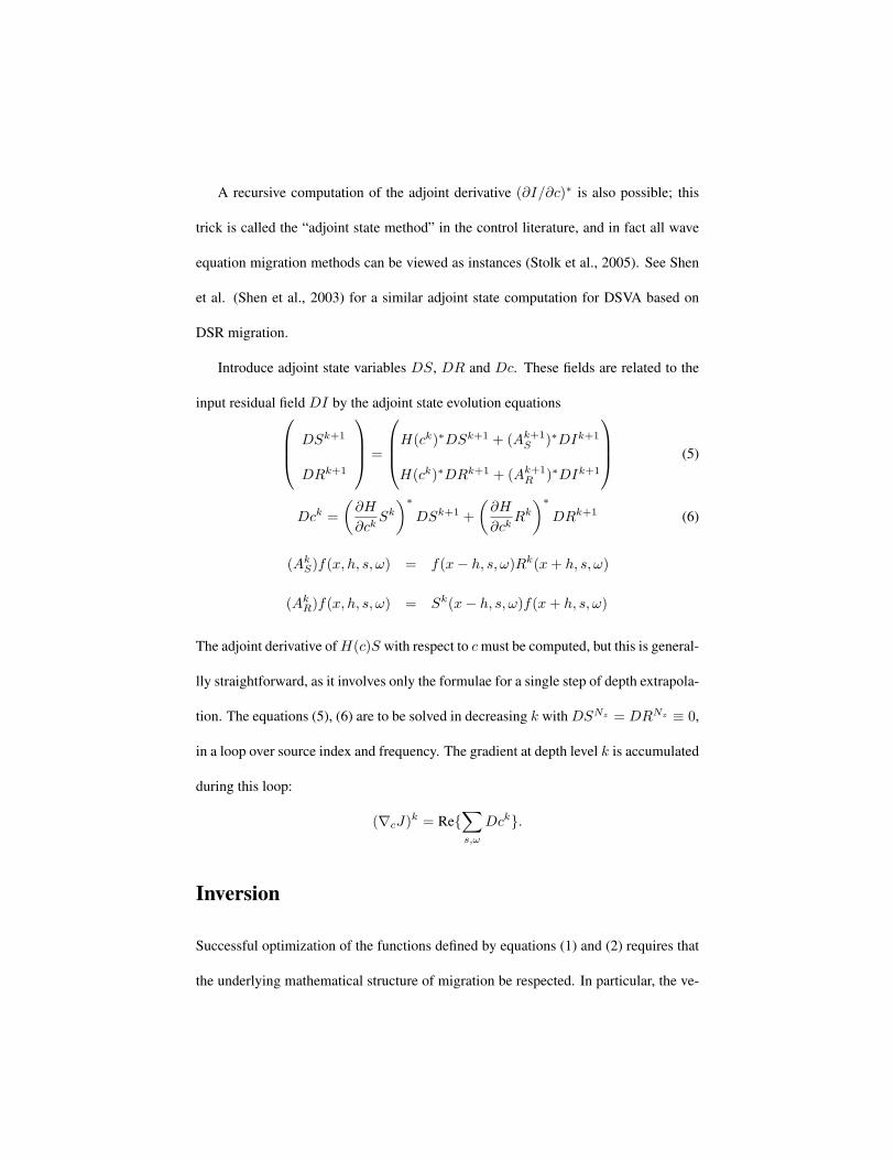
A recursive computation of the adjoint derivative (∂I/∂c)∗ is also possible; this

trick is called the “adjoint state method” in the control literature, and in fact all wave

equation migration methods can be viewed as instances (Stolk et al., 2005). See Shen

et al. (Shen et al., 2003) for a similar adjoint state computation for DSVA based on

DSR migration.

Introduce adjoint state variables DS, DR and Dc. These fields are related to the

input residual field DI by the adjoint state evolution equations DSk+1

DRk+1

=

H(ck)∗DSk+1 + (Ak+1S )∗DIk+1

H(ck)∗DRk+1 + (Ak+1R )∗DIk+1

(5)

Dck =(∂H

∂ckSk)∗

DSk+1 +(∂H

∂ckRk)∗

DRk+1 (6)

(AkS)f(x, h, s, ω) = f(x− h, s, ω)Rk(x+ h, s, ω)

(AkR)f(x, h, s, ω) = Sk(x− h, s, ω)f(x+ h, s, ω)

The adjoint derivative ofH(c)S with respect to cmust be computed, but this is general-

lly straightforward, as it involves only the formulae for a single step of depth extrapola-

tion. The equations (5), (6) are to be solved in decreasing k with DSNz = DRNz ≡ 0,

in a loop over source index and frequency. The gradient at depth level k is accumulated

during this loop:

(∇cJ)k = Re{∑s,ω

Dck}.

Inversion

Successful optimization of the functions defined by equations (1) and (2) requires that

the underlying mathematical structure of migration be respected. In particular, the ve-

locities encountered during the iteration must remain smooth on the wavelength scale.

To enforce this smoothness, we use a B-spline representation based on a relatively

coarse spacing of spline nodes. Let m be a set of B-spline model parameters and B the

B-spline sampling operator (onto the image grid). Restriction to velocities of the form

c = Bm gives a gradient in the spline parameters of the form

∇mJ(Bm) = B∗∇cJ(c)

(here J = Jh or Jθ). We use a version of limited BFGS algorithm (Nocedal and

Wright, 2000) to minimize J as a function of m. Only J and its gradient with respect

m is needed. We have now completely described the computation of these quantities.

Synthetic examples

We constructed data consistent with the model underlying DSVA by smoothing the

Marmousi model using a lowpass filter that removes any length scale smaller than 25m.

The difference between the original and smoothed models served as the reflectivity γ.

Synthetic Born data is expressed via the downgoing one-way Green’s functions of the

smoothed velocity G+ via

d(r, s, ω) =∫G+(x, s, ω)G+(x, r, ω)γ(x)dx, (7)

and can also be computed by solving a corresponding depth extrapolation problem.

The simulation is made to acquire the same number of shots as the original Marmousi

dataset: the source locations span uniformly from 2.625km to 8.975km at the spacing

of 0.025km. The receiver arrays are fixed for each shot and cover the entire surface

with spacing 0.01km. The migration is performed using frequencies from 3.3 to 40

Hz on square grids of 0.01km each side. Note that use of this data in an inversion test

commits an “inverse crime”: the data completely agrees with the model on which the

inversion is based.

Fig.12 shows the initial velocity model used in the inversion, obtained by smooth-

ing the Marmousi model using a B-spline fitting with length scale of 2.25km by 1km

(horizontal by vertical), much coarser than the resolution required for accurate imaging

(see Fig.8) of the Marmousi data set (Versteeg, 1993).

Forty seven iterations of BFGS resulted in the models displayed in Figures (13)

and (15). The fault block structure in the middle region has emerged in both cases; the

difference appear to be subtle. The image from offset domain DSVA (Figure (9)) is a

very accurate rendition of the structure of the actual Marmousi model, in all important

respects. The angle domain image (Figure (16)) is of distinctly lower quality. Compar-

ison of angle gathers (Figures (14), (17)) leads to the same conclusion: offset domain

DSVA appears to have been more successful, given the expended amount of compu-

tational effort. Note that the angle gather displayed in Figure (14) is a postprocess

result.

The reason for this difference in performance lies in the numerical condition of

the Hessian operator. The operator Pθ is of order 1/2 (in 2D!), meaning that it scales

Fourier components by the square root of frequency. The operator Ph, on the other

hand, is bounded, i.e. does not enhance high frequency components. As a result, the

Hessian (second derivative) operator of Jh is better conditioned than the Hessian of

Jθ (finite vs. infinite condition). Convergence for Newton-like methods is heavily

influenced by Hessian condition (Nocedal and Wright, 2000).

Modified scheme

The mathematical underpinning of DSVA is the same as that of prestack depth mi-

gration, namely the asymptotic theory of single or Born scattering about transparent

(smooth) background models (Symes, 2008). Unsurprisingly, the behaviour of the

algorithm degenerates as the wave propagation regime moves away from the theoreti-

cally justified arena for DSVA. A full waveform simulation of a reflection survey over

the original Marmousi model (Figure(18)) provides a good example of this deteriora-

tion in DSVA performance. We used full accoustic waveform simulation (rather than

demigration or forward Born simulation) to generate data with the same acquisition

parameters as in the previous section. Precisely the same inititial model as shown in

Figure(12) has been used to perform DSVA on this rough Marmousi data, but with

substantially finer attempted resolution, in an effort to estimate velocity features not

much larger than a wavelength. Velocity models with substantial variance at wave-

length and near-wavelength scales are not transparent, and the theoretical justification

for focussing-driven updates is in doubt. Indeed, the DSVA velocity estimates devi-

ate significantly from the true model: they are contaminated by many strong artifacts

(Figure(20),(21)), and do not produce particularly focused gathers. Note that multiple

reflection does not appear to be the cause of this pathology: this model, over the time

interval (3 s) of simulation, does not produce substantial multiply reflected energy. In-

stead, the source of the misbehaviour is the attempt to extend the DSVA method to

estimate near-wavelength scale heterogeneities, which are not transparent but which

are necessary to fully explain the kinematics of single scattering for this model.

On the other hand, the longer-scale structure of these models is improved over that

of the initial estimate, which suggests a possible modification of DSVA to extend its

domain of validity, by combining the differential semblance objective with one based

on image power. In contrast to DSVA, image power maximization makes constructive

velocity updates only when the initial velocity is reasonably accurate. However veloc-

ities estimated by maximizing image power are relatively insensitive to noise: image

power is strongly peaked at kinematically accurate velocities. Maximization of image

power was explored by Toldi (Toldi, 1989), and more recently by Soubaras (Soubaras

and Gratacos, 2007), who illustrates the robustness of the method by application to

field data.

These observations suggest that DSVA might be combined with image power anal-

ysis to yield a method with the robust global convergence of DSVA (not trapped by

local minima far from an optimal velocity) and the robust local convergence of image

power analysis (not trapped by local mimina close - but not close enough - to optimal).

Such a combined method has been implemented by Chauris (Chauris and Noble, 2001)

using common offset Kirchhoff migration as the underlying imaging method. The first

author has introduced a similar method in the context of depth extrapolation migration

(Shen and Calandra, 2005).

Motivated by these considerations, we introduce the modified DSVA objective:

J =12||hI(x, h)||2 − β2

2||I(x, 0)||. (8)

Notice the imaging power term βI(x, 0), β > 0 contains no information of image other

than h = 0, whereas the original DSVA term contains all information of image except

at h = 0. The combination produces a complete coverage of information of image in

all offsets computed.

We compute gradient of the modified objective function using the same adjoint

state approach explained above for pure DSVA. All of the formulas explained before

hold with one small modification: we need only redefine the image residual to be

DI = h2I(x, h)− β2I(x, 0). (9)

We applied this modified DSVA method to the rough Marmousi data with the same

starting model (Figure(12)) and the same set of parameters associated with the differ-

ential semblance term. Stably converged results are shown for 49 and 99 iterations

(Figures (22) (23), (24), 25)). The additional robustness of the image power term,

which is active when the model is close to kinematically correct, leads to a rather pre-

cise final velocity estimate and very satisfactory image.

Real data examples

We have applied this implementation of modified DSVA to a segment of an 2D marine

seismic line which covers a distance of about 97 kft. The preprocessing includes first

arrival removal and tau-p deconvolution-based free surface multiple removal. Surface

offsets range from 900 ft to about 10,000 ft with 81 ft source and receiver spacing.

The challenge of this data lies in the middle of the model where a vertical narrow gas

cloud is expected. As shown in Figure (27), when migration with a v(z) velocity model

produces an artificial image sag.

A ray-based reflection tomography velocity model was obtained (Figure (28) using

this data set. The migrated image (Figure (30) is more interpretable than that obtained

using the v(z) velocity (Figure 27). One of the interpretation concerns remains, how-

ever: the shape of the low velocity zone is inconsistent with the surrounding geological

setting.

Before we started the DSVA run stream, we have applied a source plane-wave phase

encoding to this data. With 60 plane waves, the data is reduced to 20% of its original

size (in frequency representation). The speed up by a factor of 5 is a significant ad-

vantage, in view of the repeated migrations required for BFGS iterations. The image

of plane-wave migration shows virtually no visible difference compared to shot-record

migration under the same one-way propagator. The offset common image gathers and

DSVA gradient are produced in the same fashion as in shot-record migration except

that the shot-record is replaced by plane-wave-records. We conducted 20 iterations of

modified DSVA updates in offset domain with a (steepest descent) restart at the 6th

iteration. The starting velocity as shown in Figure (26), is linearly increasing in depth.

We chose this starting model in order to test the robustness of DSO scheme when start-

ing model is reasonably far from the expected realistic model. In terms of compactness

of the gas cloud, the velocity model obtained from the optimization noticeably agrees

more with the geological interpretation (Figure (28) and Figure (29)). Moreover, the

images below the gas cloud (Figure (31)) show more continuity compared with the

tomography result (Figure (30)).

Once the image gathers in offset are computed, a slant stack (Sava and Fomel,

2003) can be applied to convert them to angle gathers. In general, the flatter the event

the closer the velocity model approaches the true one. Figures (32)-(34) demonstrate

increased degree of flatness in angle gathers from the image obtained at v(z) velocity,

tomography velocity to modified DSVA optimized velocity. An aparant gap in the

vicinities of zero degree for each angle gather reflects the missing of zero (surface)

offset in data.

Conclusion

Both offset and angle domain versions of DSVA are effective in updating a complex ve-

locity model involving strong refraction, though the offset domain variant as presented

here is somewhat more computationally efficient. Either supplementing the operator

Pθ with a negative order factor, for 2D, or computing in 3D where Pθ is bounded,

would likely remove the comparative advantage of the offset domain computation.

The first test demonstrated here used “perfect” data, that is, data corresponding

precisely to the theory underlying DSVA. It achieve nearly perfect results. The second

test, which transgressed the assumed scale dichotomy underlying the theory, revealed

a limitation of DSVA: even absent multiply reflected energy, the method on its own has

limited ability to resolve rapidly changing velocity features of kinematic importance.

We showed how to adjoin an image power term to the DSVA objective function; the

modified DSVA method so obtained exhibits considerably more stability in the pres-

ence of important short-scale velocity variation.

Finally, we applied the modified DSVA method to a gas sag problem for which

a reflection tomography velocity estimate is available. The modified DSVA result is

more kinematically consistent with the data (more focused image gathers) than is the

reflection tomography result, and yields a more interpretable image.

Many open questions remain concerning the sensitivity of the approach to data

imperfections, on the one hand, and the possibility of similar approaches based on

more sophisticated modeling, on the other. Previous work has shown that DSVA is

quite sensitive to the presence of multiply reflected energy (eg. (Verm and Symes,

2006)). This is hardly surprising, as the method is relies for its theoretical justification

on the single scattering assumption. Various methods have been proposed to reduce the

sensitivity of DSVA to multiples and other coherent noise (Gockenbach and Symes,

1999; Mulder and ten Kroode, 2002a; Li and Symes, 2007). The ultimate remedy may

lie in inclusion of multiple reflection in the underlying model of wave propagation -

see Symes (Symes, 2008) for a suggestion along these lines.

Acknowledgement

This work was partly supported by The Rice Inversion Project. The author wish to

thank Scott Morton for his extensive advice and many valuble suggestions, and Biondo

Biondi, Maarten de Hoop, Christiaan Stolk, and Richard Verm for many useful and

inspiring discussions on the topics of seismic inversion and velocity analysis.

References

Chauris, H. and M. Noble, 2001, Two-dimensional velocity macro model estimation

from seismic reflection data by local differential semblance optimization: applica-

tions synthetic and real data sets: Geophys. J. Int., 144, 14–26.

Foss, S. k., B. Ursin, and M. V. de Hoop, 2004, Depth-consistent p - and s - wave

velocity reflection tomography using pp and ps seismic data: Expanded Abstracts,

Society of Exploration Geophysicists, 53rd Annual International Meeting, 2363–

2367.

Gockenbach, M. and W. Symes, 1999, Coherent noise suppression in velocity inver-

sion: 69th Annual International Meeting, Expanded Abstracts, 1719–1723, Society

of Exploration Geophysicists.

Kabir, N., U. Albertin, M. Zhou, V. Nagassar, E. Kjos, and P. Whittaker, 2007, Use

of refraction, reflection and wave-equation-based tomography for imaging beneath

the shallow gas: a Trinidad field data example: 77th Annual International Meeting,

Expanded Abstracts, 2812–2815, Society of Exploration Geophysicists.

Kern, M. and W. Symes, 1994, Inversion of reflection seismograms by differential

semblance analysis: Algorithm structure and synthetic examples: Geophysical

Prospecting, 565–614.

Li, J. and W. Symes, 2007, Interval velocity estimation via nmo-based differential sem-

blance: Geophysics, 72, U75–U88.

Mulder, W. and A. ten Kroode, 2002a, Automatic velocity analysis by differential sem-

blance optimization: Geophysics, 67, 1184–1191.

Mulder, W. A. and A. P. E. ten Kroode, 2002b, Automatic velocity analysis by differ-

ential semblance optimization: Geophysics, 67, 1184–1191.

Nocedal, J. and S. Wright, 2000, Numerical optimization: Springer Verlag.

Sava, P. and S. Fomel, 2003, Angle domain common-image gathers by wavefield con-

tinuation methods: Geophysics, 68, 1065–1074.

Shen, P. and H. Calandra, 2005, One-way waveform inversion within the framwork

of adjoint state differential migration: Expanded Abstracts, Society of Exploration

Geophysicists, 75th Annual International Meeting (submitted).

Shen, P., C. Stolk, and W. Symes, 2003, Automatic velocity analysis by differential

semblance optimization: Expanded Abstracts, Society of Exploration Geophysi-

cists, 73rd Annual International Meeting, 2132–2135.

Soubaras, R. and B. Gratacos, 2006, Velocity model building by semblance maximiza-

tion of modulated-shot gathers: 76th Annual International Meeting, Expanded Ab-

stracts, SVIP1.3, Society of Exploration Geophysicists.

——–, 2007, Velocity model building by semblancemaximization of modulated-shot

gathers: Geophysics, 72, U67.

Stolk, C. and W. Symes, 2004, Kinematic aritifacts in prestack depth migration: Geo-

physics, 69, 562–575.

Stolk, C. C., M. V. de hoop, and W. W. Symes, 2005, Kinematics of shot-geophone mi-

gration: Technical Report 05-04, Department of Computational and Applied Math-

ematics, Rice University, Houston, Texax, USA.

Symes, W., 1986, Stability and instability results for inverse problems in several-

dimensional wave propagation in glowinski, r., and lions, j.: Proc. 7th International

Conference on Computing Methods in Applied Science and Engineering:: North-

Holland, 69.

Symes, W. and R. Versteeg, 1993, Velocity model determination using differential

semblance optimization: expanded Abstracts, Society of Exploration Geophysicists,

63rd Annual International Meeting, 696–699.

Symes, W. W., 2008, Migration velocity analysis and waveform inversion: Geophysical

Prospecting, 56, (in press).

Toldi, J., 1989, Velocity analysis without picking: Geophysics, 54, 191–199.

Verm, R. and W. Symes, 2006, Practice and pitfalls in NMO-based differential sem-

blance velocity analysis: 75th Annual International Meeting, Expanded Abstracts,

SI3.7, Society of Exploration Geophysicists.

Versteeg, R. J., 1993, Sensitivity of prestack depth migration to the velocity model:

Geophysics, 58, 873–882.

Captions

Figure(1). A smoothed version of the Marmousi velocity model, considered as a “true”

model for this study. The horizontal velocity variability is kept at a length scale greater

than 120 metesr.

Figure(2). A reflectivity distribution map γ(x) obtained by high pass filtering the orig-

inal Marmousi velocity model.

Figure(3). Data in time simulated by finite difference time stepping. Velocity used is

the superposition of the background velocity and the reflectivity distribution, as shown

in figure(1) and figure(2), respectively. Events beyond the first arrivals are muted.

Figure(4). Data in time simulated by the one-way propagator according to equation(7)

with reflecting boundary condition. Events beyond the direct arrivals are muted. Al-

though the amplitudes do not agree with that obtained from the time simulation, the

reflection events are modeled at the correct time.

Figure(5). The image obtained through a perfect pre-stack depth migration at the “true”

velocity as shown in figure(1), where the migration propagator completely agrees with

the modeling propagator.

Figure(6). The migrated offset gathers, picked from the center of the model, obtained

through pre-stack depth migration at the “true” velocity as shown in figure(1). The

offset ranges from -0.5km to 0.5km with an interval of 0.01km for each gather. The en-

ergy is clearly seen to be concentrated, to the leading order, at the center of the gather.

Figure(7). The angle gathers obtained through a “Fomel/Sava” Radon transform from

the offset gathers as shown in figure(6). The flatness angle indicates an alternative mea-

surement of the accuracy of the velocity as oppose to the concentration in offset.

Figure(12). The starting velocity model obtained by the B-spline projection corre-

sponds to a horizontal length scale of 1.3 km.

Figure(8). The initial image at the starting velocity model. Significant distortion of the

image, particularly in the deeper part of the model, is due the presence of large velocity

error.

Figure(10). The initial offset gather at the starting velocity model. Although the data

is strictly one-way Born, the energy is disperssive across the range of offsets modeled,

indicating the missing of strong refracting structures in the starting model.

Figure(9). Image by optimized velocity of offset domain DSVA at 47th iteration.

Figure(13). Optimized velocity by offset domain DSVA at 47th iteration.

Figure(11). Offset gathers by offset domain DSVA at 47th iteration. They are well

focused at h = 0.

Figure(14). The angle gathers obtained through a “Fomel/Sava” Radon transform from

the optimized offset gathers as shown in figure(11). As the offset gathers become fo-

cused, the corresponding angle gathers become flat.

Figure(16). The image obtained by the angle domain DSVA. The image shows more

distortion compared with that of the offset domain DSVA (figure(9)).

Figure(15). The optimized velocity through angle domain DSVA. It shows more vari-

abilities compared with figure(13).

Figure(17). The angle gathers through angle domain DSVA. It is clear that they are not

as flat in comparison with those obtained from the offset domain DSVA (figure(14)).

Figure(19). Initial image at the v(z) velocity model (figure(12)). Although obtained at

different data, similar features are shown compared to figure(8).

Figure(20). Velocity output of DSVA to rough Marmousi data at 49th interation. The

inherited roughness of velocity in the data makes the optmization problem more diffi-

cult.

Figure(21). Velocity output of DSVA to rough Marmousi data at 82th interation. Fea-

tures of the correct Marmousi velocity model are burried under many artifacts. As the

number of iterations increase, these artifacts become stronger.

Figure(22). Velocity output of modifed DSVA at 49th interation. It shows close resem-

blance to the true Marmousi model. The imaging power term plays an important role

to stablize the results.

Figure(23). Image output of modified DSVA at 49th interation. Compared to the initial

image (figure(19)), significant coherent engergies are recollected for deeper images.

Figure(24). Velocity output of modifed DSVA at 99th interation. As the number of

iterations increases, the velocity estimate kept stable.

Figure(25). Image output of modified DSVA at 99th interation. The image continues

to improve as the optmization continues.

Figure(26). Initial v(z) velocity model. To test the roubustness of DSVA, we take

the average velocity of the first and the last layer from best the tomography velocity

(figure(28)) and linearly interpolate for all depths to creat this v(z) veloity model.

Figure(27). Image at the initial v(z) velocity.

Figure(28). The optimized velocity output by ray tracing tomography which is per-

formed independently. Vertical and horizontal units are 1000 feets.

Figure(29). The velocity output by modified offset domain DSVA at 20th iteration.

The starting model is shown in figure(26). Vertical and horizontal units are 1000 feets.

Figure(30). Image obtained at the optimized velocity of ray tracing tomography.

Figure(31). Image by optimized velocity of modified offset domain DSVA.

Figure(32). Angle gathers by Radon transform from offset gathers at the initial v(z)

velocity model.

Figure(33). Angle gathers by Radon transform from offset gathers at the optimized

velocity of ray tracing tomography.

Figure(34). Angle gathers by Radon transform from offset gathers at the velocity out-

put of modified offset domain DSVA at 20th iteration.

Fig. 1: Smoothed ”true” velocity model.

Fig. 2: Singular reflectivity model.

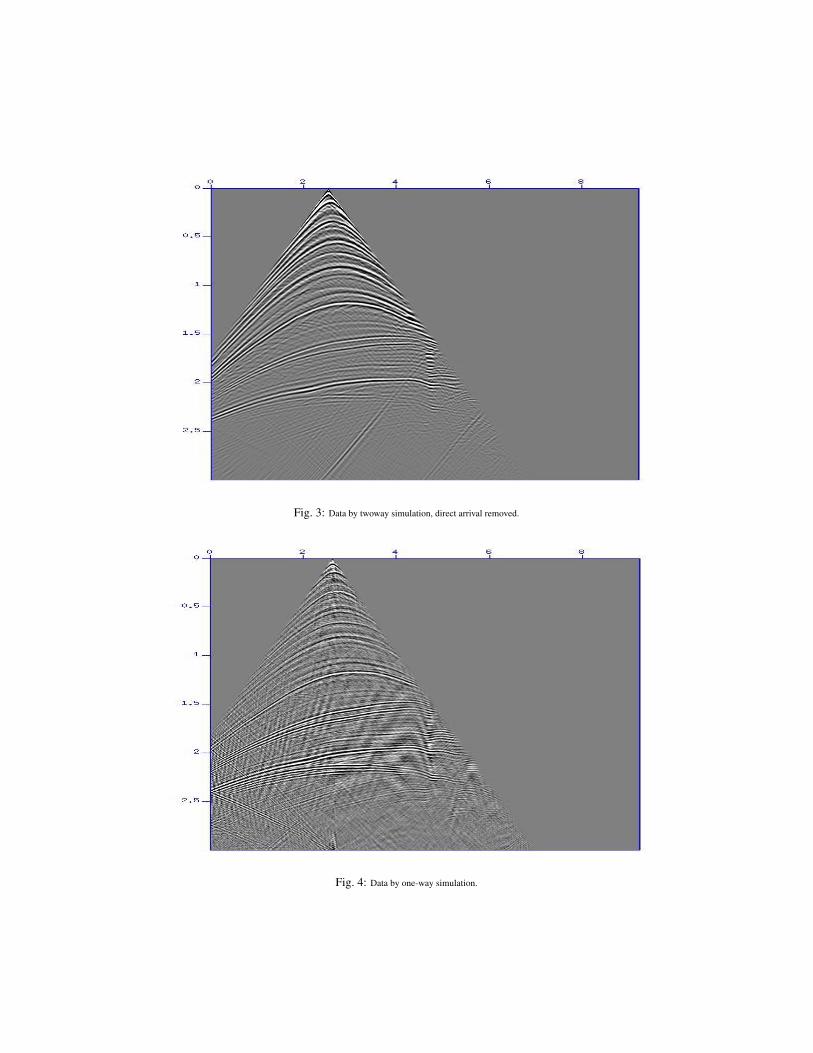
Fig. 3: Data by twoway simulation, direct arrival removed.

Fig. 4: Data by one-way simulation.

Fig. 5: Image at true velocity model.

Fig. 6: Offset gathers obtained at the true velocity model.

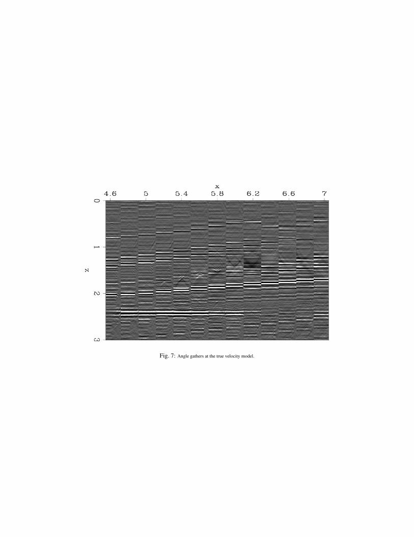
Fig. 7: Angle gathers at the true velocity model.

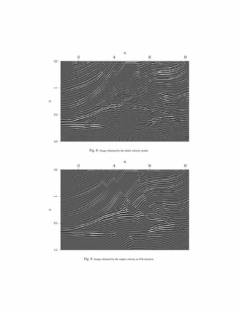
Fig. 8: Image obtained by the initial velocity model.

Fig. 9: Image obtained by the output velocity at 47th iteration.

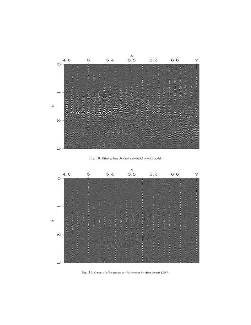
Fig. 10: Offset gathers obtained at the initial velocity model.

Fig. 11: Output of offset gathers at 47th iteration by offset domain DSVA.

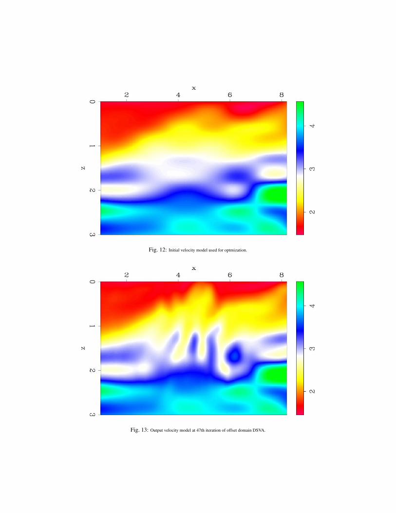
Fig. 12: Initial velocity model used for optmization.

Fig. 13: Output velocity model at 47th iteration of offset domain DSVA.

Fig. 14: Angle gathers by optmized velocity of offset domain DSVA.

Fig. 15: Optimized velocity model by angle domain DSVA.

Fig. 16: Image by optmized velocity of angle domain DSVA.

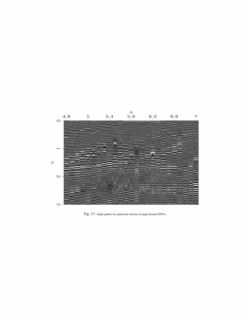
Fig. 17: Angle gathers by optimized velocity of angle domain DSVA.

Fig. 18: Unsmoothed Marmousi velocity model.

Fig. 19: Initial image velocity as shown in figure(12).

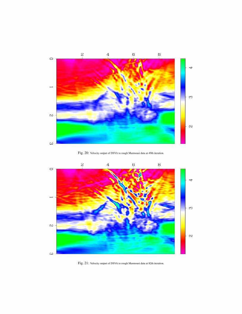
Fig. 20: Velocity output of DSVA to rough Marmousi data at 49th iteration.

Fig. 21: Velocity output of DSVA to rough Marmousi data at 82th iteration.

Fig. 22: Velocity output of modified DSVA at 49th iteration.

Fig. 23: Image output of modified DSVA at 49th iteration.

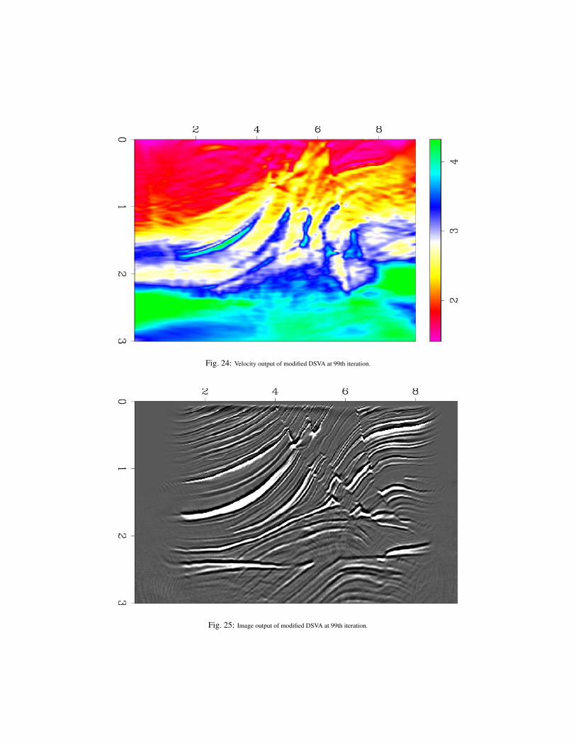
Fig. 24: Velocity output of modified DSVA at 99th iteration.

Fig. 25: Image output of modified DSVA at 99th iteration.

Fig. 26: Initial v(z) velocity model for real data optimization.

Fig. 27: Initial image by v(z) velocity.

Fig. 28: Optimized velocity by ray tracing tomography.

Fig. 29: Optimized velocity by modified DSVA.

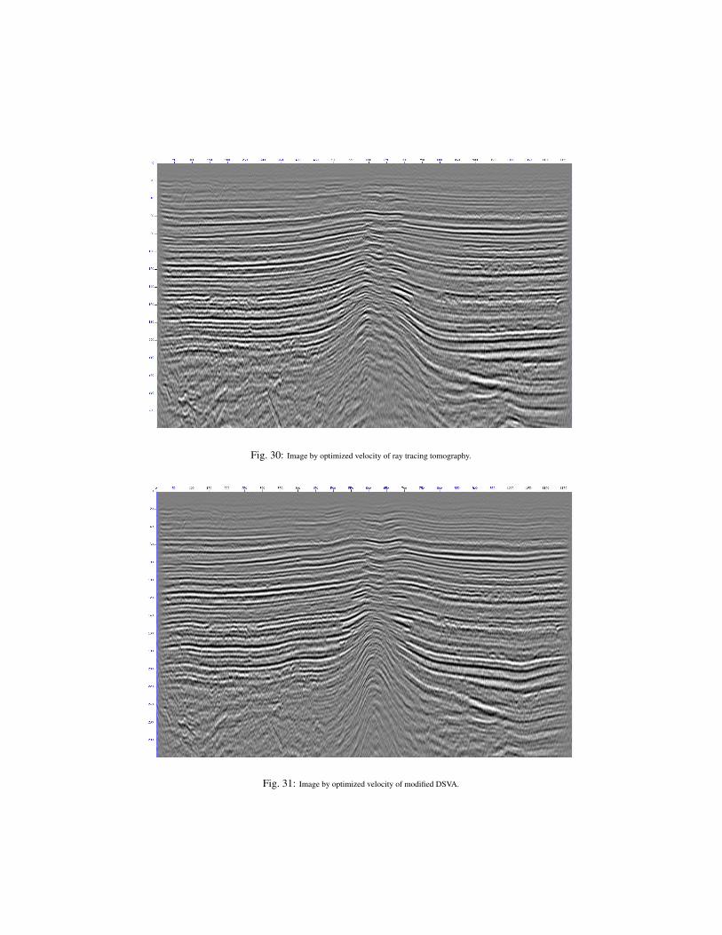
Fig. 30: Image by optimized velocity of ray tracing tomography.

Fig. 31: Image by optimized velocity of modified DSVA.

Fig. 32: Initial angle gather by v(z) velocity.

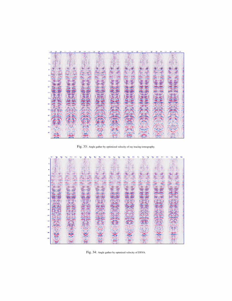
Fig. 33: Angle gather by optimized velocity of ray tracing tomography.

Fig. 34: Angle gather by optmized velocity of DSVA.