IT 09 008

Examensarbete 45 hpMarch 2009

Automatic Verification of Dynamic Data-Dependent Programs

Ran Ji

Institutionen för informationsteknologiDepartment of Information Technology

Teknisk- naturvetenskaplig fakultet UTH-enheten Besöksadress: Ångströmlaboratoriet Lägerhyddsvägen 1 Hus 4, Plan 0 Postadress: Box 536 751 21 Uppsala Telefon: 018 – 471 30 03 Telefax: 018 – 471 30 00 Hemsida: http://www.teknat.uu.se/student

Abstract

Automatic Verification of Dynamic Data-DependentPrograms

Ran Ji

We present a new approach for automatic verification of data-dependent programsmanipulating dynamic heaps. A heap is encoded by a graph where the nodes representthe cells, and the edges reflect the pointer structure between the cells of the heap.Each cell contains a set of variables which range over the natural numbers. Ourmethod relies on standard backward reachability analysis, where the main idea is touse a simple set of predicates, called signatures, in order to represent bad sets ofheaps. Examples of bad heaps are those which contain either garbage, lists which arenot well-formed, or lists which are not sorted. We present the results for the case ofprograms with a single next-selector, and where variables may be compared forequality or inequality. This allows us to verify for instance that a program, like bubblesort or insertion sort, returns a list which is well-formed and sorted, or that themerging of two sorted lists is a new sorted list. We will report on the result ofrunning a prototype based on the method on a number of programs.

Tryckt av: Reprocentralen ITCIT 09 008Examinator: Anders JanssonÄmnesgranskare: Parosh AbdullaHandledare: Jonathan Cederberg

Acknowledgements

First of all, I would like to give the greatest thanks to my reviewer Prof.

Parosh Aziz Abdulla. Thank you for giving me the opportunity to do

my master thesis in the APV group, for your excellent lectures Program-

ming Theory and Data Structures, which led me to the magic world of

verification, and for your patience and encouragement.

Secondly, my warm thanks goes to Jonathan Cederberg, who is not only

my thesis supervisor but also a sincere friend. I will always remember the

inspirated discussions and enjoyable teamworks. The work will never be

like now without you.

Thirdly, it is a pleasure for me to share the room with Muhsin Haji Atto,

who has been with me all along the thesis work. I am also grateful to the

other members of the APV group: Frederic Haziza, Noomene Ben Henda,

Lisa Kaati, Ahmed Rezine and Mayank Saksena.

I have had many interesting courses in IT department, thanks to all the

teachers. In particular, I would like to mention Prof. Bengt Jonsson and

Prof. Wang Yi. They offered me more than the knowledge given in class.

My friends in Uppsala also help me a lot in both life and studying, thanks.

Last but not least, I owe my thanks to my parents. Their endless love and

instant supporting give me the courage to overcome every difficulty and

make me trust myself all the time. I wish to make you proud.

Contents

1 Introduction 1

1.1 Introduction . . . . . . . . . . . . . . . . . . . . . . . . . . . . . . . . 1

1.2 Related Work . . . . . . . . . . . . . . . . . . . . . . . . . . . . . . . 3

1.3 Outline . . . . . . . . . . . . . . . . . . . . . . . . . . . . . . . . . . . 4

2 Heaps 6

2.1 Heaps . . . . . . . . . . . . . . . . . . . . . . . . . . . . . . . . . . . 6

2.2 Programming Language . . . . . . . . . . . . . . . . . . . . . . . . . 8

2.3 Transition System . . . . . . . . . . . . . . . . . . . . . . . . . . . . . 9

3 Signatures 12

3.1 Signatures . . . . . . . . . . . . . . . . . . . . . . . . . . . . . . . . . 12

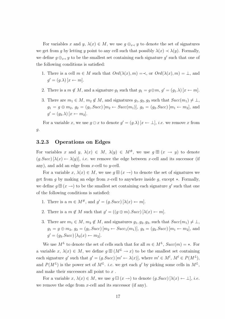
3.2 Operations on Signatures . . . . . . . . . . . . . . . . . . . . . . . . . 14

3.2.1 Operations on Cells . . . . . . . . . . . . . . . . . . . . . . . . 14

3.2.2 Operations on Variables . . . . . . . . . . . . . . . . . . . . . 15

3.2.3 Operations on Edges . . . . . . . . . . . . . . . . . . . . . . . 17

3.2.4 Operation on Ordering Relations . . . . . . . . . . . . . . . . 18

3.3 Ordering . . . . . . . . . . . . . . . . . . . . . . . . . . . . . . . . . . 18

4 Bad Configurations 20

4.1 Sorted Linear List . . . . . . . . . . . . . . . . . . . . . . . . . . . . . 20

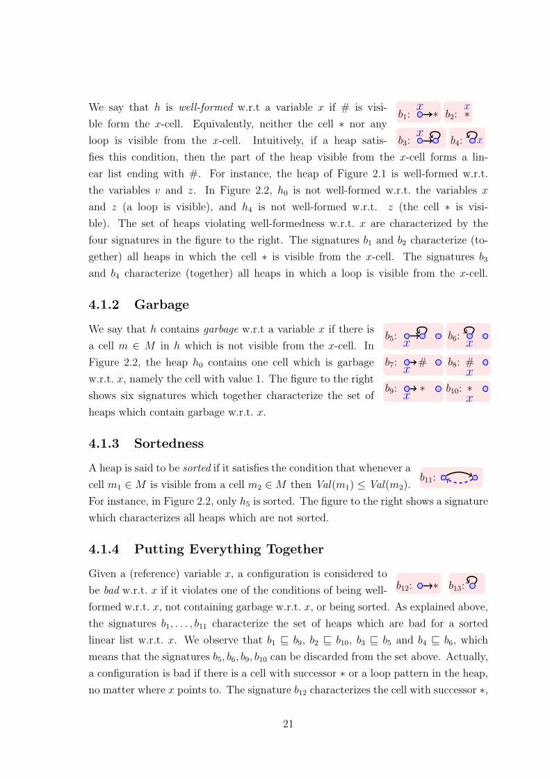
4.1.1 Well-Formedness . . . . . . . . . . . . . . . . . . . . . . . . . 20

4.1.2 Garbage . . . . . . . . . . . . . . . . . . . . . . . . . . . . . . 21

4.1.3 Sortedness . . . . . . . . . . . . . . . . . . . . . . . . . . . . . 21

4.1.4 Putting Everything Together . . . . . . . . . . . . . . . . . . . 21

4.2 Sorted Cyclic List . . . . . . . . . . . . . . . . . . . . . . . . . . . . . 22

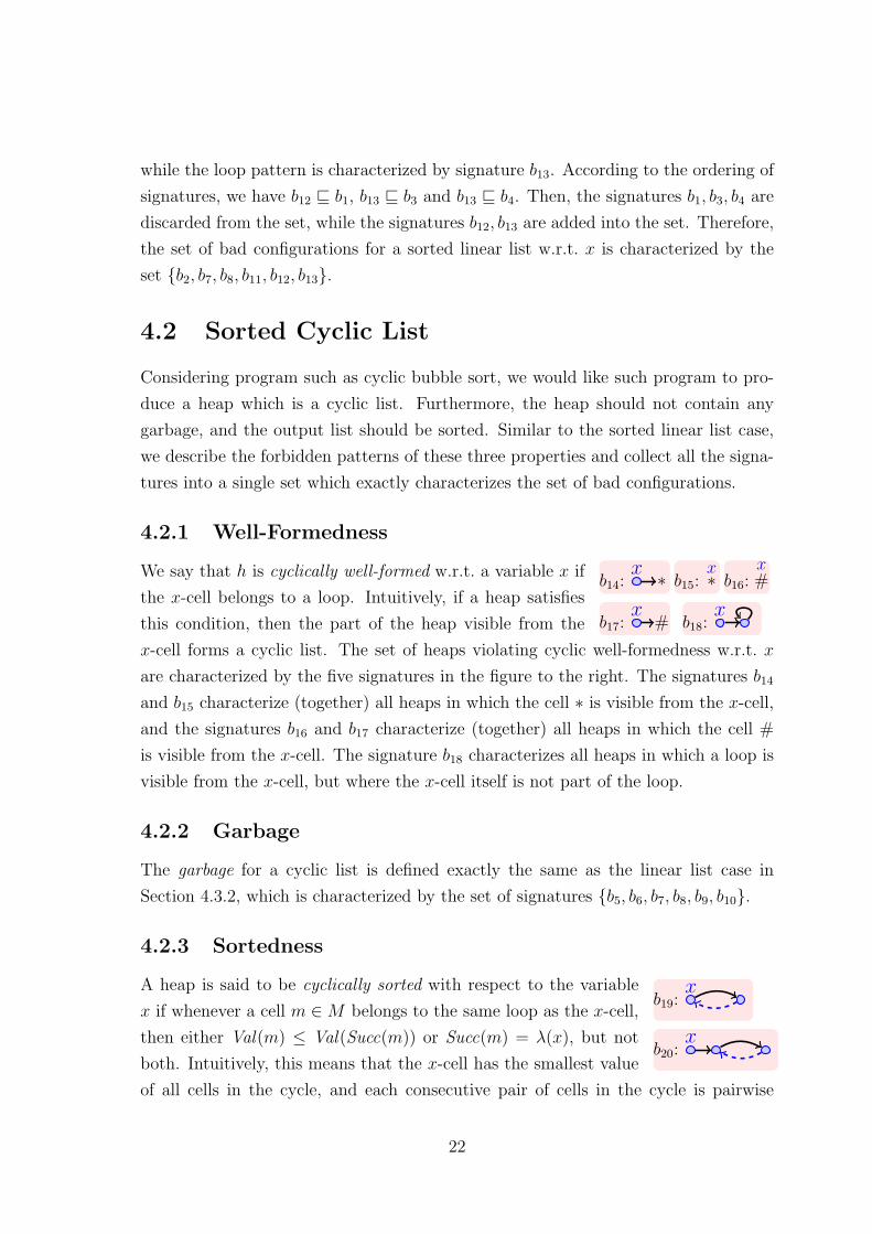
4.2.1 Well-Formedness . . . . . . . . . . . . . . . . . . . . . . . . . 22

4.2.2 Garbage . . . . . . . . . . . . . . . . . . . . . . . . . . . . . . 22

4.2.3 Sortedness . . . . . . . . . . . . . . . . . . . . . . . . . . . . . 22

i

4.2.4 Putting Everything Together . . . . . . . . . . . . . . . . . . . 23

4.3 Sorted Partition . . . . . . . . . . . . . . . . . . . . . . . . . . . . . . 23

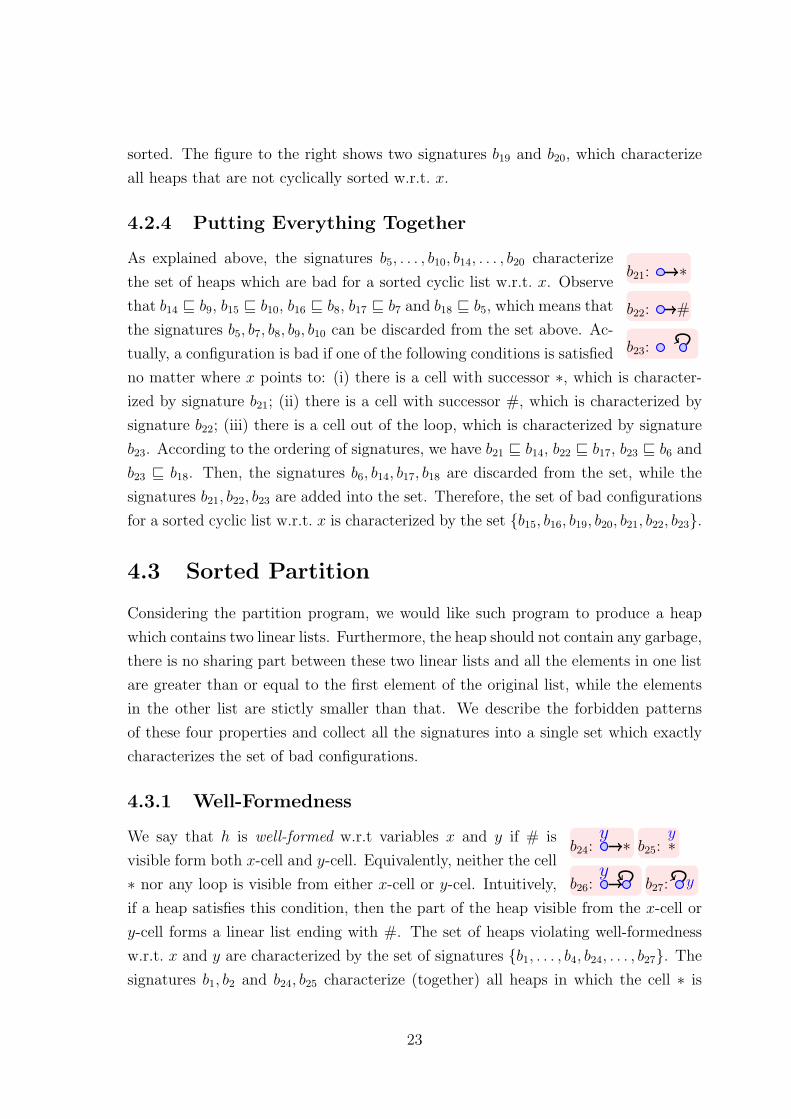
4.3.1 Well-Formedness . . . . . . . . . . . . . . . . . . . . . . . . . 23

4.3.2 Garbage . . . . . . . . . . . . . . . . . . . . . . . . . . . . . . 24

4.3.3 Sharing . . . . . . . . . . . . . . . . . . . . . . . . . . . . . . 24

4.3.4 Sortedness . . . . . . . . . . . . . . . . . . . . . . . . . . . . . 24

4.3.5 Putting Everything Together . . . . . . . . . . . . . . . . . . . 24

4.4 More Bad on Inverse Sortedness . . . . . . . . . . . . . . . . . . . . . 25

4.4.1 Inversely Sorted Linear List . . . . . . . . . . . . . . . . . . . 25

4.4.2 Inversely Sorted Cyclic List . . . . . . . . . . . . . . . . . . . 25

5 Reachability Analysis 26

5.1 Over-Approximation . . . . . . . . . . . . . . . . . . . . . . . . . . . 26

5.2 Computing Predecessors . . . . . . . . . . . . . . . . . . . . . . . . . 26

5.3 Initial Heaps . . . . . . . . . . . . . . . . . . . . . . . . . . . . . . . . 32

5.4 Checking Safety Properties . . . . . . . . . . . . . . . . . . . . . . . . 32

5.4.1 Reachability Algorithm . . . . . . . . . . . . . . . . . . . . . . 32

5.4.2 Checking Entailment . . . . . . . . . . . . . . . . . . . . . . . 33

5.4.3 Searching Strategies . . . . . . . . . . . . . . . . . . . . . . . 35

6 Experimental Results 36

6.1 Example Programs . . . . . . . . . . . . . . . . . . . . . . . . . . . . 36

6.1.1 Insert . . . . . . . . . . . . . . . . . . . . . . . . . . . . . . . 36

6.1.2 Insert(bug) . . . . . . . . . . . . . . . . . . . . . . . . . . . . 36

6.1.3 Merge . . . . . . . . . . . . . . . . . . . . . . . . . . . . . . . 36

6.1.4 Reverse . . . . . . . . . . . . . . . . . . . . . . . . . . . . . . 38

6.1.5 ReverseCyclic . . . . . . . . . . . . . . . . . . . . . . . . . . . 38

6.1.6 Partition . . . . . . . . . . . . . . . . . . . . . . . . . . . . . . 38

6.1.7 BubbleSort . . . . . . . . . . . . . . . . . . . . . . . . . . . . 40

6.1.8 BubbleSort(bug) . . . . . . . . . . . . . . . . . . . . . . . . . 41

6.1.9 BubbleSortCyclic . . . . . . . . . . . . . . . . . . . . . . . . . 41

6.1.10 InsertionSort . . . . . . . . . . . . . . . . . . . . . . . . . . . 42

6.2 Experimental Results . . . . . . . . . . . . . . . . . . . . . . . . . . . 42

7 Conclusions and Future Work 44

ii

List of Figures

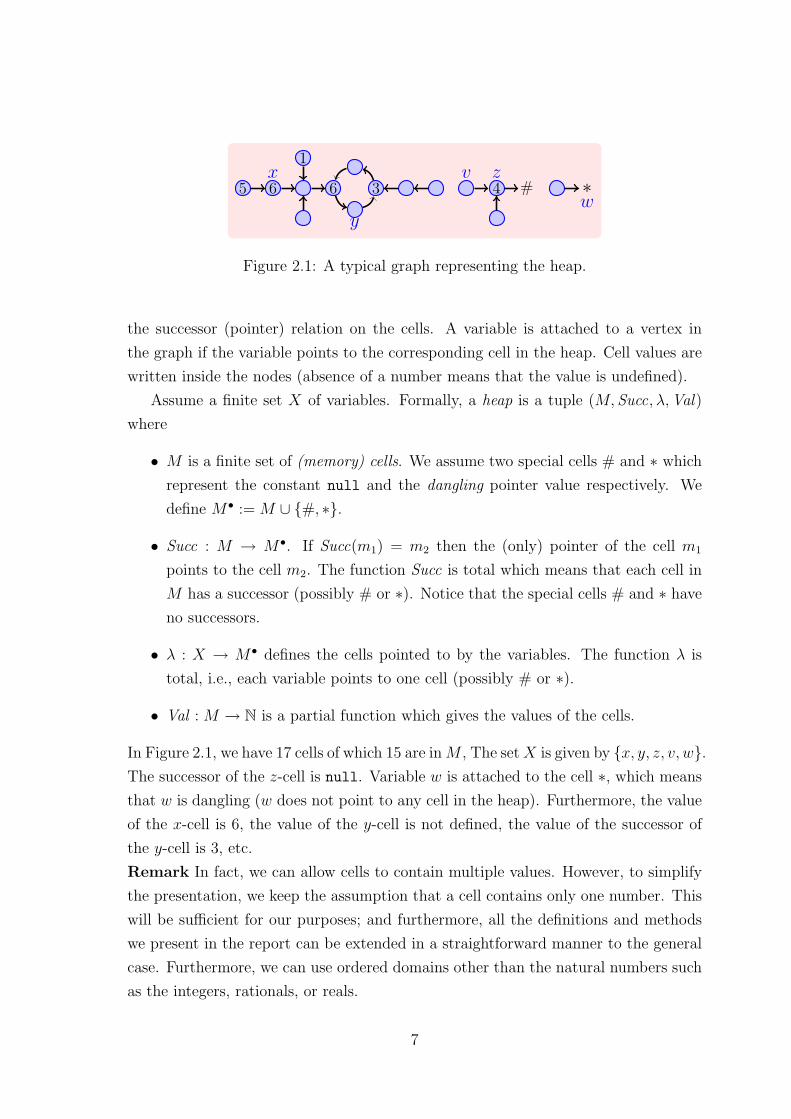
2.1 A typical graph representing the heap. . . . . . . . . . . . . . . . . . 7

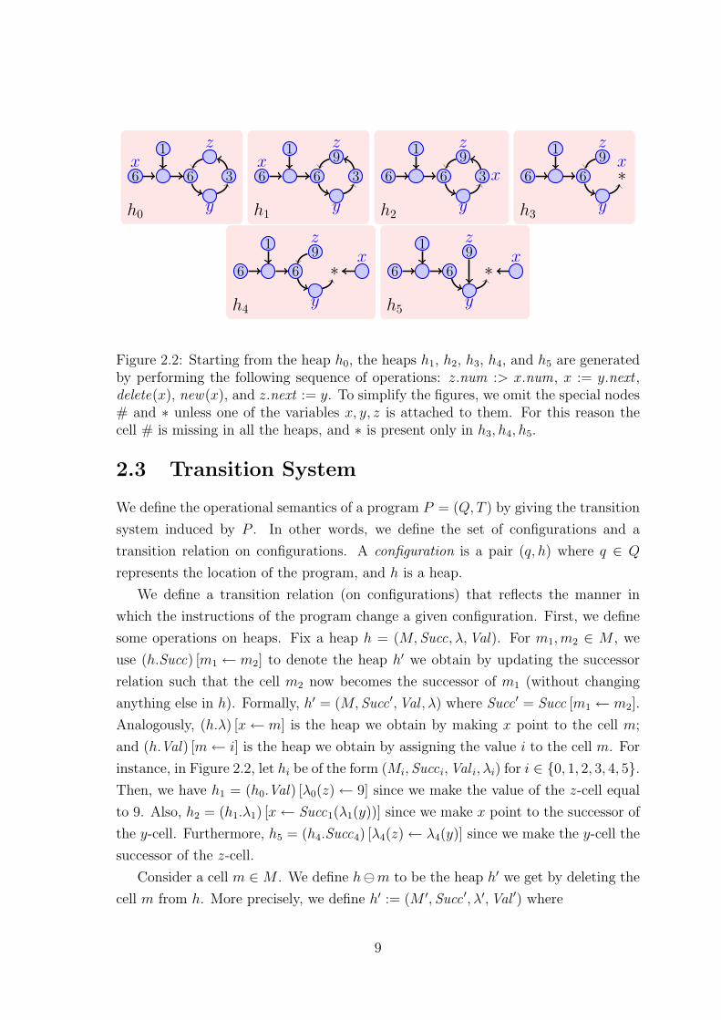
2.2 Starting from the heap h0, the heaps h1, h2, h3, h4, and h5 are generated

by performing the following sequence of operations: z.num :> x.num,

x := y.next , delete(x), new(x), and z.next := y. To simplify the

figures, we omit the special nodes # and ∗ unless one of the variables

x, y, z is attached to them. For this reason the cell # is missing in all

the heaps, and ∗ is present only in h3, h4, h5. . . . . . . . . . . . . . 9

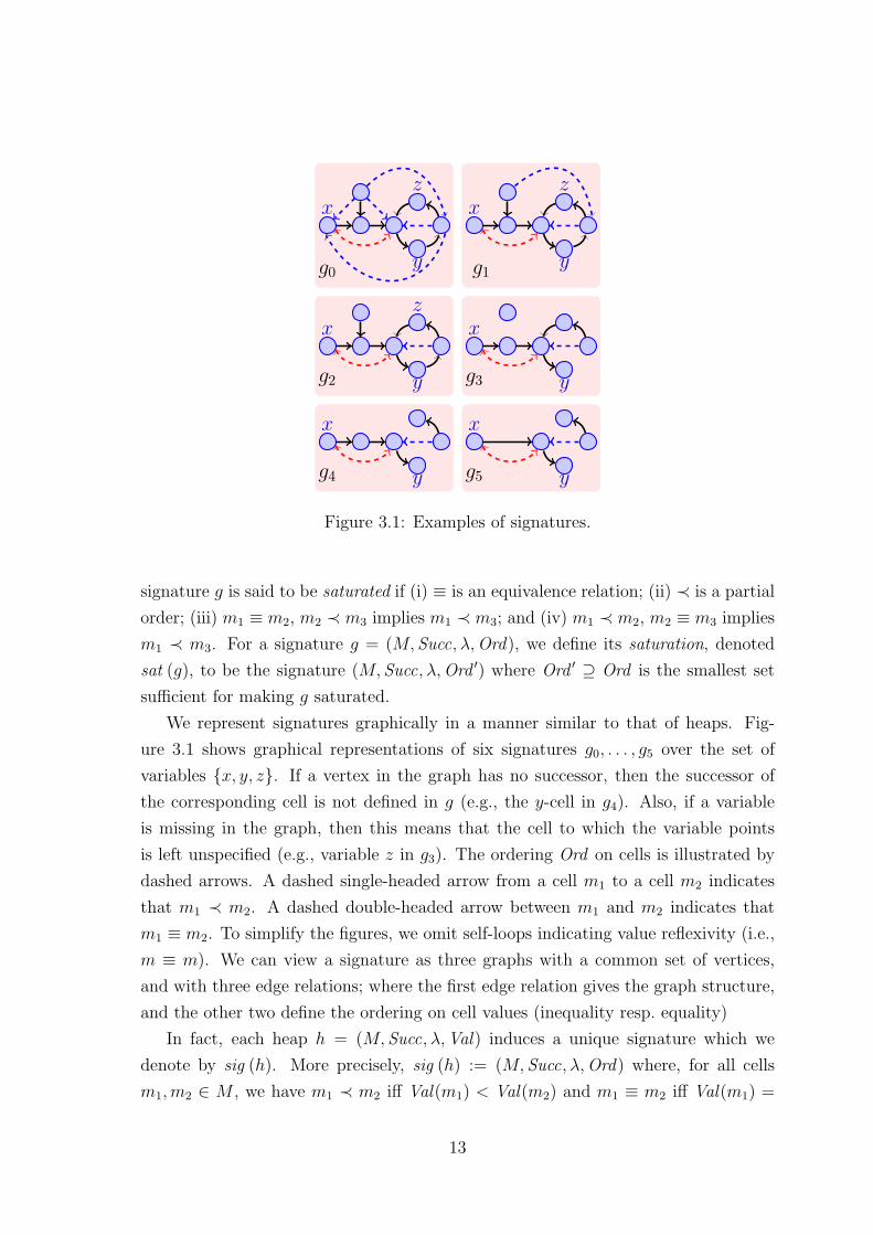
3.1 Examples of signatures. . . . . . . . . . . . . . . . . . . . . . . . . . . 13

5.1 The procedure of generating a linear list . . . . . . . . . . . . . . . . 32

6.1 The insert program including initialization phase . . . . . . . . . . . 37

6.2 The merge program without initialization phase . . . . . . . . . . . . 37

6.3 The reverse program without initialization phase . . . . . . . . . . . . 38

6.4 The reverseCyclic program including initialization phase . . . . . . . 39

6.5 The partition program including initialization phase . . . . . . . . . . 39

6.6 The bubbleSort program without initialization phase . . . . . . . . . 40

6.7 The bubbleSortCyclic program including initialization phase . . . . . 41

6.8 The insertionSort program without initialization phase . . . . . . . . 42

iii

iv

Chapter 1

Introduction

1.1 Introduction

We consider automatic verification of data-dependent programs that manipulate dy-

namic linked lists. The contents of the linked lists, here refered to as a heap, is

represented by a graph. The nodes of the graph represent the cells of the heap, while

the edges reflect the pointer structure between the cells (see Figure 2.1 for a typical

example). The program has a dynamic behaviour in the sense that cells may be

created and deleted; and that pointers may be re-directed during the execution of

the program. The program is also data-dependent since the cells contain variables,

ranging over the natural numbers, that can be compared for (in)equality and whose

values may be updated by the program. The values of the local variables are provided

as attributes to the corresponding cells. Finally, we have a set of (pointer) variables

which point to different cells inside the heap.

In this report, we consider the case of programs with a single next-selector, i.e.,

where each cell has at most one successor. For this class of programs, we provide a

method for automatic verification of safety properties. Such properties can be either

structural properties such as absence of garbage, sharing, and dangling pointers; or

data properties such as sortedness. We provide a simple symbolic representation,

which we call signatures, for characterizing (infinite) sets of heaps. Signatures can

also be represented by graphs. The difference, compared to the case of heaps, is

that some parts may be “missing” from the graph of a signature. For instance, the

absence of a pointer means that the pointer may point to an arbitrary cell inside a

heap satisfying the signature. In this manner, a signature can be interpreted as a

forbidden pattern which should not occur inside the heap. The forbidden pattern is

essentially a set of minimal conditions which should be satisfied by any heap in order

for the heap to satisfy the signature. A heap satisfying the signature is considered

1

to be bad in the sense that it contains a bad pattern which in turn implies that it

violates one of the properties mentioned above. Examples of bad patterns in heaps

are garbage, lists which are not well-formed, or lists which are not sorted. This means

that checking a safety property amounts to checking the reachability of a finite set

of signatures. We perform standard backward reachability analysis, using signatures

as a symbolic representation, and starting from the set of bad signatures. We show

how to perform the two basic operations needed for backward reachability analysis,

namely checking entailment and computing predecessors on signatures.

For checking entailment, we define a pre-order v on signatures, where we view a

signature as three separate graphs with identical sets of nodes. The edge relation in

one of the three graphs reflects the structure of the heap graph, while the other two

reflect the ordering on the values of the variables (equality resp. inequality). Given

two signatures g1 and g2, we have g1 v g2 if g1 can be obtained from g2 by a sequence

of transformations consisting of either deleting an edge (in one of the three graphs), a

variable, an isolated node, or contracting segments (i.e., sequence of nodes) without

sharing in the structure graph. In fact, this ordering also induces an ordering on

heaps where h1 v h2 if, for all signatures g, h2 satisfies g whenever h1 satisfies g.

When performing backward reachability analysis, it is essential that the underly-

ing symbolic representation, signatures in our case, is closed under the operation of

computing predecessors. More precisely, for a signature g, let us define Pre(g) to be

the set of predecessors of g, i.e., the set of signatures which characterize those heaps

from which we can perform one step of the program and as a result obtain a heap

satisfying g. Unfortunately, the set Pre(g) does not exist in general under the oper-

ational semantics of the class of programs we consider in this report. Therefore, we

consider an over-approximation of the transition relation where a heap h is allowed

first to move to smaller heap (w.r.t. the ordering v) before performing the transition.

For the approximated transition relation, we show that the set Pre(g) exists, and that

it is finite and computable.

One advantage of using signatures is that it is quite straightforward to specify

sets of bad heaps. For instance, forbidden patterns for the properties of list well-

formedness and absence of garbage can each be described by 4-6 signatures, with 2-3

nodes in each signature. Also, the forbidden pattern for the property that a list is

sorted consists of only one signature with two nodes. Furthermore, signatures offer

a very compact symbolic representation of sets of bad heaps. In fact, when verifying

our programs, the number of nodes in the signatures which arise in the analysis does

not exceed ten. In addition, the rules for computing predecessors are local in the

2

sense that they change only a small part of the graph (typically one or two nodes and

edges). This makes it possible to check entailment and compute predecessors quite

efficiently.

The whole verification process is fully automatic since both the approximation

and the reachability analysis are carried out without user intervention. Notice that if

we verify a safety property in the approximate transition system then this also implies

its correctness in the original system. We have implemented a prototype based on our

method, and carried out automatic verification of several programs such as insertion

in a sorted lists, bubble sort, insertion sort, merging of sorted lists, list partitioning,

reversing sorted lists, etc. Although the procedure is not guaranteed to terminate in

general, our prototype terminates on all these examples.

1.2 Related Work

Several works consider the verification of singly linked lists with data. The paper [11]

presents a method for automatic verification of sorting programs that manipulate

linked lists. The method is defined within the framework of TVLA which provides

an abstract description of the heap structures in 3-valued logic [16]. The user may be

required to provide instrumentation predicates in order to make the abstraction suffi-

ciently precise. The analysis is performed in a forward manner. In contrast, the search

procedure we describe in this report is backward, and therefore also property-driven.

Thus, the signatures obtained in the traversal do not need to express the state of the

entire heap, but only those parts that contribute to the eventual failure. This makes

the two methods conceptually and technically different. Furthermore, the difference

in search strategy implies that forward and backward search procedures often offer

varying degrees of efficiency in different contexts, which makes them complementary

to each other in many cases. This has been observed also for other models such as

parameterized systems, timed Petri nets, and lossy channel systems (see e.g. [3, 8, 1]).

Another approach to verification of linked lists with data is proposed in [5, 6] based

on abstract regular model checking (ARMC) [7]. In ARMC, finite-state automata are

used as a symbolic representation of sets of heaps. This means that the ARMC-based

approach needs the manipulation of quite complex encodings of the heap graphs

into words or trees. In contrast, our symbolic representation uses signatures which

provide a simpler and more natural representation of heaps as graphs. Furthermore,

ARMC uses a sophisticated machinery for manipulating the heap encodings based on

representing program statements as (word/tree) transducers. However, as mentioned

3

above, our operations for computing predecessors are all local in the sense that they

only update limited parts of the graph thus making it possible to have much more

efficient implementations.

The paper [4] uses counter automata as abstract models of heaps which contain

data from an ordered domain. The counters are used to keep track of lengths of list

segments without sharing. The analysis reduces to manipulation of counter automata,

and thus requires techniques and tools for these automata.

Recently, there has been an extensive work to use separation logic [15] for per-

forming shape analysis of programs that manipulate pointer data structures (see e.g.

[9, 18]). The paper [13] describes how to use separation logic in order to provide a

semi-automatic procedure for verifying data-dependent programs which manipulate

heaps. In contrast, the approach we present here uses a built-in abstraction princi-

ple which is different from the ones used above and which makes the analysis fully

automatic.

The tool PALE (Pointer Assertion Logic Engine) [12] checks automatically prop-

erties of programs manipulating pointers. The user is required to supply assertions

expressed in the weak monadic second-order logic of graph types. This means that the

verification procedure as a whole is only partially automatic. The tool MONA [10],

which uses translations to finite-state automata, is employed to verify the provided

assertions.

In our previous work [2], we used backward reachability analysis for verifying

heap manipulating programs. However, the programs are restricted to be data-

independent. The extension to the case of data-dependent programs is not trivial

and requires an intricate treatment of the ordering on signatures. In particular, the

interaction between the structural and the data orderings is central to our method.

This is used for instance to specify basic properties like sortedness (whose forbid-

den pattern contains edges from both orderings). Hence, none of the programs we

consider in this report can be analyzed in the framework of [2].

1.3 Outline

In the next chapter, we describe our model of heaps, and introduce the programming

language together with the induced transition system. In Chapter 3, we introduce the

notion of signatures and the associated ordering. Chapter 4 describes how to specify

sets of bad heaps using signatures. In Chapter 5 we give an overview of the backward

reachability scheme, and show how to compute the predecessor relation on signatures.

4

The experimental results are presented in Chapter 6. Finally, in Chapter 7 we give

some conclusions and directions for future research.

5

Chapter 2

Heaps

In this chapter, we give some preliminaries on programs which manipulate heaps.

Let N be the set of natural numbers. For sets A and B, we write f : A → B

to denote that f is a (possibly partial) function from A to B. We write f(a) = ⊥to denote that f(a) is undefined. We use f [a← b] to denote the function f ′ such

that f ′(a) = b and f ′(x) = f(x) if x 6= a. In particular, we use f [a← ⊥] to denote

the function f ′ which agrees on f on all arguments, except that f ′(a) is undefined.

A binary relation R on a set A is said to be a partial order if it is irreflexive and

transitive. We say that R is an equivalence relation if it is reflexive, symmetric, and

transitive. We use f(a).= f(b) to denote that f(a) 6= ⊥, f(b) 6= ⊥, and f(a) = f(b),

i.e., f(a) and f(b) are defined and equal. Analogously, we write f(a)lf(b) to denote

that f(a) 6= ⊥, f(b) 6= ⊥, and f(a) < f(b).

2.1 Heaps

We consider programs which operate on dynamic data structures, here called heaps.

A heap consists of a set of memory cells (cells for short), where each cell has one

next-pointer. Examples of such heaps are singly liked lists and circular lists, possibly

sharing their parts (see Figure 2.1). A cell in the heap may contain a datum which

is a natural number. A program operating on a heap may use a finite set of variables

representing pointers whose values are cells inside the heap. A pointer may have

the special value null which represents a cell without successors. Furthermore, a

pointer may be dangling which means that it does not point to any cell in the heap.

Sometimes, we write the “x-cell” to refer to the the cell pointed to by the variable

x. We also write “the value of the x-cell” to refer to the value stored inside the

cell pointed to by x. A heap can naturally be encoded by a graph, as the one of

Figure 2.1. A vertex in the graph represents a cell in the heap, while the edges reflect

6

5 6x

1

6

y

3v

4z

# ∗w

Figure 2.1: A typical graph representing the heap.

the successor (pointer) relation on the cells. A variable is attached to a vertex in

the graph if the variable points to the corresponding cell in the heap. Cell values are

written inside the nodes (absence of a number means that the value is undefined).

Assume a finite set X of variables. Formally, a heap is a tuple (M, Succ, λ,Val)

where

• M is a finite set of (memory) cells. We assume two special cells # and ∗ which

represent the constant null and the dangling pointer value respectively. We

define M• := M ∪ {#, ∗}.

• Succ : M → M•. If Succ(m1) = m2 then the (only) pointer of the cell m1

points to the cell m2. The function Succ is total which means that each cell in

M has a successor (possibly # or ∗). Notice that the special cells # and ∗ have

no successors.

• λ : X → M• defines the cells pointed to by the variables. The function λ is

total, i.e., each variable points to one cell (possibly # or ∗).

• Val : M → N is a partial function which gives the values of the cells.

In Figure 2.1, we have 17 cells of which 15 are inM , The setX is given by {x, y, z, v, w}.The successor of the z-cell is null. Variable w is attached to the cell ∗, which means

that w is dangling (w does not point to any cell in the heap). Furthermore, the value

of the x-cell is 6, the value of the y-cell is not defined, the value of the successor of

the y-cell is 3, etc.

Remark In fact, we can allow cells to contain multiple values. However, to simplify

the presentation, we keep the assumption that a cell contains only one number. This

will be sufficient for our purposes; and furthermore, all the definitions and methods

we present in the report can be extended in a straightforward manner to the general

case. Furthermore, we can use ordered domains other than the natural numbers such

as the integers, rationals, or reals.

7

2.2 Programming Language

We define a simple programming language. To this end, we assume, together with the

earlier mentioned set X of variables, the constant null where null 6∈ X. We define

X# := X ∪ {null}. A program P is a pair (Q, T ) where Q is a finite set of control

states and T is a finite set of transitions. The control states represent the locations

of the program. A transition is a triple (q1, op, q2) where q1, q2 ∈ Q are control states

and op is an operation. In the transition, the program changes location from q1 to

q2, while it checks and manipulates the heap according to the operation op. The

operation op is of one of the following forms

• x = y or x 6= y where x, y ∈ X#. The program checks whether the x- and

y-cells are identical or different.

• x := y or x.next := y where x ∈ X and y ∈ X#. In the first operation, the

program makes x point to the y-cell, while in the second operation it updates

the successor of the x-cell, and makes it equal to the y-cell.

• x := y.next where x, y ∈ X. The variable x will now point to the successor of

the y-cell.

• new(x), delete(x), or read(x ), where x ∈ X. The first operation creates a new

cell and makes x point to it; the second operation removes the x-cell from the

heap; while the third operation reads a new value and assigns it to the x-cell.

• x.num = y.num, x.num < y.num, x.num := y.num, x.num :> y.num, or

x.num :< y.num, where x, y ∈ X. The first two operations compare the val-

ues of (number stored inside) the x- and y-cells. The third operation copies

the value of the y-cell to the x-cell. The fourth (fifth) operation assigns non-

deterministically a value to the x-cell which is larger (smaller) than that of the

y-cell.

Figure 2.2 illustrates the effect of a sequence of operations of the forms described

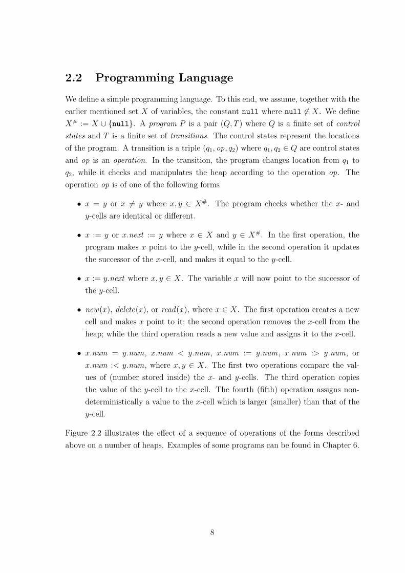
above on a number of heaps. Examples of some programs can be found in Chapter 6.

8

6x

1

6

y

z

3

h0

6x

1

6

y

9z

3

h1

6

1

6

y

9z

3 x

h2

6

1

6

y

9z

∗x

h3

6

1

6

y

9z

∗x

h4

6

1

6

y

9z

∗x

h5

Figure 2.2: Starting from the heap h0, the heaps h1, h2, h3, h4, and h5 are generatedby performing the following sequence of operations: z.num :> x.num, x := y.next ,delete(x), new(x), and z.next := y. To simplify the figures, we omit the special nodes# and ∗ unless one of the variables x, y, z is attached to them. For this reason thecell # is missing in all the heaps, and ∗ is present only in h3, h4, h5.

2.3 Transition System

We define the operational semantics of a program P = (Q, T ) by giving the transition

system induced by P . In other words, we define the set of configurations and a

transition relation on configurations. A configuration is a pair (q, h) where q ∈ Q

represents the location of the program, and h is a heap.

We define a transition relation (on configurations) that reflects the manner in

which the instructions of the program change a given configuration. First, we define

some operations on heaps. Fix a heap h = (M, Succ, λ,Val). For m1,m2 ∈ M , we

use (h.Succ) [m1 ← m2] to denote the heap h′ we obtain by updating the successor

relation such that the cell m2 now becomes the successor of m1 (without changing

anything else in h). Formally, h′ = (M, Succ ′,Val , λ) where Succ ′ = Succ [m1 ← m2].

Analogously, (h.λ) [x← m] is the heap we obtain by making x point to the cell m;

and (h.Val) [m← i] is the heap we obtain by assigning the value i to the cell m. For

instance, in Figure 2.2, let hi be of the form (Mi, Succi,Val i, λi) for i ∈ {0, 1, 2, 3, 4, 5}.Then, we have h1 = (h0.Val) [λ0(z)← 9] since we make the value of the z-cell equal

to 9. Also, h2 = (h1.λ1) [x← Succ1(λ1(y))] since we make x point to the successor of

the y-cell. Furthermore, h5 = (h4.Succ4) [λ4(z)← λ4(y)] since we make the y-cell the

successor of the z-cell.

Consider a cell m ∈M . We define hm to be the heap h′ we get by deleting the

cell m from h. More precisely, we define h′ := (M ′, Succ ′, λ′,Val ′) where

9

• M ′ = M − {m}.

• Succ ′(m′) = Succ(m′) if Succ(m′) 6= m, and Succ ′(m′) = ∗ otherwise. In other

words, the successor of cells pointing to m will become dangling in h′.

• λ′(x) = ∗ if λ(x) = m, and λ′(x) = λ(x) otherwise. In other words, variables

pointing to the same cell as x in h will become dangling in h′.

• Val ′(m′) = Val(m′) if m′ ∈ M ′. That is, the function Val ′ is the restriction of

Val to M ′: it assigns the same values as Val to all the cells which remain in M ′

(since m 6∈M ′, it not meaningful to speak about Val (m)).

In Figure 2.2, we have h3 = h2 λ2(x).

Let t = (q1, op, q2) be a transition and let c = (q, h) and c′ = (q′, h′) be config-

urations. We write ct−→ c′ to denote that q = q1, q

′ = q2, and hop−→ h′, where

hop−→ h′ holds if we obtain h′ by performing the operation op on h. For heaps h and

h′, hop−→ h′ holds if one of the following conditions is satisfied:

• op is of the form x = y, λ(x) 6= ∗, λ(y) 6= ∗, λ(x) = λ(y), and h′ = h. In other

words, the transition is enabled if the pointers are not dangling, and they point

to the same cell.

• op is of the form x 6= y, λ(x) 6= ∗, λ(y) 6= ∗, λ(x) 6= λ(y), and h′ = h.

• op is of the form x := y, λ(y) 6= ∗, and h′ = (h.λ) [x← λ(y)].

• op is of the form x := y.next , λ(y) ∈M , Succ(λ(y)) 6= ∗, and h′ = (h.λ) [x← Succ(λ(y))].

• op is of the form x.next := y, λ(x) ∈M , λ(y) 6= ∗, and h′ = (h.Succ) [λ(x)← λ(y)].

• op is of the from new(x), M ′ = M ∪ {m} for some m 6∈ M , λ′ = λ [x← m],

Succ ′ = Succ [m← ∗], Val ′(m′) = Val(m′) if m′ 6= m, and Val ′(m) = ⊥. This

operation creates a new cell and makes x point to it. The value of the new cell

is not defined, while the successor is the special cell ∗.

• op is of the form delete(x), λ(x) ∈M , and h′ = hλ(x). The operation deletes

the x-cell.

• op is of the form read(x ), λ(x) ∈ M , and h′ = (h.Val) [λ(x)← i ], where i is

the value assigned to x-cell.

10

• op is of the form x.num = y.num, λ(x) ∈M , λ(y) ∈M , Val(λ(x)).= Val(λ(y)),

and h′ = h. The transition is enabled if the pointers are not dangling and the

values of their cells are defined and equal.

• op is of the form x.num < y.num, λ(x) ∈M , λ(y) ∈M , Val(λ(x))l Val(λ(y)),

and h′ = h.

• op is of the form x.num := y.num, λ(x) ∈ M , λ(y) ∈ M , Val(λ(y)) 6= ⊥, and

h′ = (h.Val) [λ(x)← Val(λ(y))].

• op is of the form x.num :> y.num, λ(x) ∈ M , λ(y) ∈ M , Val(λ(y)) 6= ⊥, and

h′ = (h.Val) [λ(x)← i], where i > Val(λ(y)). The case for x.num :< y.num is

defined analogously.

We write c −→ c′ to denote that ct−→ c′ for some t ∈ T ; and use

∗−→ to denote the

reflexive transitive closure of −→. The relations −→ and∗−→ are extended to sets of

configurations in the obvious manner.

Remark One could also allow deterministic assignment operations of the form x.num :=

y.num + k or x.num := y.num − k for some constant k. However, according the ap-

proximate transition relation which we define in Chapter 5, these operations will have

identical interpretations as the non-deterministic operations given above.

11

Chapter 3

Signatures

In this chapter, we introduce the notion of signatures. We will define an ordering on

signatures from which we derive an ordering on heaps. We will then show how to use

signatures as a symbolic representation of infinite sets of heaps.

3.1 Signatures

Roughly speaking, a signature is a graph which is “less concrete” than a heap in the

following sense:

• We do not store the actual values of the cells in a signature. Instead, we define

an ordering on the cells which reflects their values.

• The functions Succ and λ in a signature are partial (in contrast to a heap in

which these functions are total).

Formally, a signature g is a tuple of the form (M, Succ, λ,Ord), where M , Succ, λ

are defined in the same way as in heaps (Chapter 2), except that Succ and λ are

now partial. Furthermore, Ord is a partial function from M ×M to the set {≺,≡}.Intuitively, if Succ(m) = ⊥ for some cell m ∈ M , then this means that g puts no

constraints on the successor of m, i.e., the successor of m can be any arbitrary cell.

Analogously, if λ(x) = ⊥, then x may point to any of the cells. The relation Ord

constrains the ordering on the cell values. If Ord(m1,m2) =≺ then the value of m1 is

strictly smaller than that of m2; and if Ord(m1,m2) =≡ then their values are equal.

This means that we abstract away the actual values of the cells, and only keep track of

their ordering (and whether they are equal). For a cell m, we say that the value of m is

free if Ord(m,m′) = ⊥ and Ord(m′,m) = ⊥ for all other cells m′. Abusing notation,

we write m1 ≺ m2 (resp. m1 ≡ m2) if Ord(m1,m2) =≺ (resp. Ord(m1,m2) =≡). A

12

x

y

z

g0

x

y

z

g1

x

y

z

g2

x

yg3

x

yg4

x

yg5

Figure 3.1: Examples of signatures.

signature g is said to be saturated if (i) ≡ is an equivalence relation; (ii) ≺ is a partial

order; (iii) m1 ≡ m2, m2 ≺ m3 implies m1 ≺ m3; and (iv) m1 ≺ m2, m2 ≡ m3 implies

m1 ≺ m3. For a signature g = (M, Succ, λ,Ord), we define its saturation, denoted

sat (g), to be the signature (M, Succ, λ,Ord ′) where Ord ′ ⊇ Ord is the smallest set

sufficient for making g saturated.

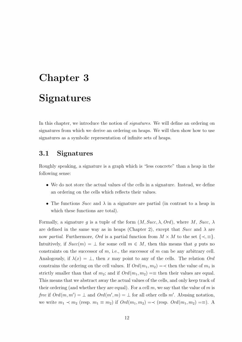
We represent signatures graphically in a manner similar to that of heaps. Fig-

ure 3.1 shows graphical representations of six signatures g0, . . . , g5 over the set of

variables {x, y, z}. If a vertex in the graph has no successor, then the successor of

the corresponding cell is not defined in g (e.g., the y-cell in g4). Also, if a variable

is missing in the graph, then this means that the cell to which the variable points

is left unspecified (e.g., variable z in g3). The ordering Ord on cells is illustrated by

dashed arrows. A dashed single-headed arrow from a cell m1 to a cell m2 indicates

that m1 ≺ m2. A dashed double-headed arrow between m1 and m2 indicates that

m1 ≡ m2. To simplify the figures, we omit self-loops indicating value reflexivity (i.e.,

m ≡ m). We can view a signature as three graphs with a common set of vertices,

and with three edge relations; where the first edge relation gives the graph structure,

and the other two define the ordering on cell values (inequality resp. equality)

In fact, each heap h = (M, Succ, λ,Val) induces a unique signature which we

denote by sig (h). More precisely, sig (h) := (M, Succ, λ,Ord) where, for all cells

m1,m2 ∈ M , we have m1 ≺ m2 iff Val(m1) < Val(m2) and m1 ≡ m2 iff Val(m1) =

13

Val(m2). In other words, in the signature of h, we remove the concrete values in the

cells and replace them by the ordering relation on the cell values. For example, in

Figure 2.2 and Figure 3.1, we have g0 = sig (h0).

3.2 Operations on Signatures

We use M# to denote M ∪{#}. Assume a saturated signature g = (M, Succ, λ,Ord).

A cell m ∈M is said to be semi-isolated if there is no x ∈ X with λ(x) = m, the value

of m is free, Succ−1(m) = ∅, and either Succ(m) = ⊥ or Succ(m) = ∗. In other words,

m is not pointed to by any variables, its value is not related to that of any other cell,

it has no predecessors, and it has no successors (except possibly ∗). We say that m is

isolated if it is semi-isolated and in addition Succ(m) = ⊥. A cell m ∈ M is said to

be simple if there is no x ∈ X with λ(x) = m, the value of m is free, |Succ−1(m)| = 1,

and Succ(m) 6= ⊥. In other words, m has exactly one predecessor, one successor and

no label. In Figure 3.1, the topmost cell of g3 is isolated, and the successor of the

x-cell in g4 is simple. In Figure 2.1, the cell to the left of the w-cell is semi-isolated

in the signature of the heap.

The operations (g.Succ) [m1 ← m2] and (g.λ) [x← m] are defined in identical fash-

ion to the case of heaps. Furthermore, for cells m1,m2 and 2 ∈ {≺,≡,⊥}, we define

(g.Ord) [(m1,m2)← 2] to be the signature g′ we obtain from g by making the order-

ing relation between m1 and m2 equal to 2.

3.2.1 Operations on Cells

For m 6∈ M , we define g ⊕m to be the signature g′ = (M ′, Succ ′, λ′,Ord ′) such that

M ′ = M ∪ {m}, Succ ′ = Succ, λ′ = λ, and Ord ′ = Ord . i.e. we add a new cell to g.

Observe that the added cell is then isolated.

We define g ⊕ λ(x) to be the signature g′ = (M ′, Succ ′, λ′,Ord ′) such that M ′ =

M ∪ {m}, Succ ′ = Succ, λ′ = λ [x← m], and Ord ′ = Ord . i.e. we add a new cell to

g which is pointed by x .

For m ∈ M , we define g m to be the signature g′ = (M ′, Succ ′, λ′,Ord ′) such

that

• M ′ = M − {m}.

• Succ ′(m′) = Succ(m′) if Succ(m′) 6= m, and Succ ′(m′) = ∗ otherwise.

• λ′(x) = ∗ if λ(x) = m, and λ′(x) = λ(x) otherwise.

14

• Ord ′(m1,m2) = Ord(m1,m2) if m1,m2 ∈M ′.

3.2.2 Operations on Variables

We use g⊕x to denote the set of signatures we get from g by letting x point anywhere

inside g, except on ∗. Formally, we define g⊕x to be the smallest set containing each

signature g′ such that one of the following conditions is satisfied:

1. There is a cell m ∈M#, and g′ = (g.λ) [x← m].

2. There is a cell m 6∈ M , and a signature g1 such that g1 = g ⊕ m, g′ =

(g1.λ) [x← m].

3. There are m1 ∈M , m2 6∈M , and signatures g1, g2, g3 such that Succ(m1) 6= ⊥,

g1 = g ⊕m2, g2 = (g1.Succ) [m2 ← Succ(m1)], g3 = (g2.Succ) [m1 ← m2], and

g′ = (g3.λ) [x← m2].

For variables x and y, λ(x) ∈M#, we use g⊕=x y to denote (g.λ) [y ← λ(x)], i.e.

we make y point to the same cell as x. Furthermore, we define g ⊕6=x y to be the

smallest set containing each signature g′ such that g′ ∈ (g⊕y), and λ′(y) 6= λ′(x), i.e.

we make y point anywhere inside g except on x-cell and ∗. As a special case, we use

g⊕6=# y to denote the smallest set containing each signature g′ such that g′ ∈ (g⊕y),

and λ′(y) 6= #, i.e. we make y point anywhere inside g except on # and ∗.For variables x and y, λ(x) ∈M , Succ(λ(x)) ∈M#, we use g⊕x→ y to denote the

set of signatures we get from g by letting y point to the successor of x-cell. Formally,

we define g ⊕x→ y to be the smallest set containing each signature g′ such that one

of the following conditions is satisfied:

1. g′ = (g.λ) [y ← Succ(λ(x))].

2. There is a cell m 6∈ M , and signatures g1, g2, g3, such that g1 = g ⊕ m, g2 =

(g1.Succ) [m← Succ1(λ(x)], g3 = (g2.Succ) [λ(x)← m], and g′ = (g3.λ) [y ← m].

for variables x and y, Succ(λ(x)) = ∗, we use g⊕x→∗ y to denote the signature we

get from g by letting y point to the new added cell in between x-cell and ∗. Formally,

we define g⊕x→∗y to be the signature g′ such that there is a cellm 6∈M , and signatures

g1, g2, g3, such that g1 = g ⊕m, g2 = (g1.Succ) [m← ∗], g3 = (g2.Succ) [λ(x)← m],

and g′ = (g3.λ) [y ← m].

For variables x and y, λ(x) ∈M#, we use g⊕x← y to denote the set of signatures

we get from g by letting y point to any cell except ∗, where it has no successor or its

15

successor is x-cell. Formally, we define g⊕x← y to be the smallest set containing each

signature g′ such that one of the following conditions is satisfied:

1. There is a cell m ∈ M such that Succ(m) = ⊥ or Succ(m) = λ(x), and

g′ = (g.λ) [y ← m].

2. There is a cell m 6∈ M , and a signature g1 such that g1 = g ⊕ m, g′ =

(g1.λ) [y ← m].

3. There are m1 ∈ M , m2 6∈ M , and signatures g1, g2, g3, such that Succ(m1) =

λ(x), g1 = g ⊕m2, g2 = (g1.Succ) [m2 ← λ(x)], g3 = (g2.Succ) [m1 ← m2], and

g′ = (g3.λ) [y ← m2].

For variables x and y, λ(x) ∈ M , we use g ⊕≡x y to denote the set of signatures

we get from g by letting y point to any cell such that possibly λ(y) ≡ λ(x). Formally,

we define g⊕≡x y to be the smallest set containing each signature g′ such that one of

the following conditions is satisfied:

1. There is a cell m ∈ M such that Ord(m,λ(x)) =≡ or Ord(m,λ(x)) = ⊥, and

g′ = (g.λ) [x← m].

2. There is a cell m 6∈ M , and a signature g1 such that g1 = g ⊕ m, g′ =

(g1.λ) [x← m].

3. There are m1 ∈M , m2 6∈M , and signatures g1, g2, g3 such that Succ(m1) 6= ⊥,

g1 = g ⊕m2, g2 = (g1.Succ) [m2 ← Succ(m1)], g3 = (g2.Succ) [m1 ← m2], and

g′ = (g3.λ) [x← m2].

For variables x and y, λ(x) ∈ M , we use g ⊕≺x y to denote the set of signatures

we get from g by letting y point to any cell such that possibly λ(y) ≺ λ(x). Formally,

we define g⊕≺x y to be the smallest set containing each signature g′ such that one of

the following conditions is satisfied:

1. There is a cell m ∈ M such that Ord(m,λ(x)) =≺, or Ord(m,λ(x)) = ⊥, and

g′ = (g.λ) [x← m].

2. There is a cell m 6∈ M , and a signature g1 such that g1 = g ⊕ m, g′ =

(g1.λ) [x← m].

3. There are m1 ∈M , m2 6∈M , and signatures g1, g2, g3 such that Succ(m1) 6= ⊥,

g1 = g ⊕m2, g2 = (g1.Succ) [m2 ← Succ(m1)], g3 = (g2.Succ) [m1 ← m2], and

g′ = (g3.λ) [x← m2].

16

For variables x and y, λ(x) ∈ M , we use g ⊕x≺ y to denote the set of signatures

we get from g by letting y point to any cell such that possibly λ(x) ≺ λ(y). Formally,

we define g⊕x≺ y to be the smallest set containing each signature g′ such that one of

the following conditions is satisfied:

1. There is a cell m ∈ M such that Ord(λ(x),m) =≺, or Ord(λ(x),m) = ⊥, and

g′ = (g.λ) [x← m].

2. There is a m 6∈M , and a signature g1 such that g1 = g⊕m, g′ = (g1.λ) [x← m].

3. There are m1 ∈M , m2 6∈M , and signatures g1, g2, g3 such that Succ(m1) 6= ⊥,

g1 = g ⊕m2, g2 = (g1.Succ) [m2 ← Succ(m1)], g3 = (g2.Succ) [m1 ← m2], and

g′ = (g3.λ) [x← m2].

For a variable x, we use gx to denote g′ = (g.λ) [x← ⊥], i.e. we remove x from

g.

3.2.3 Operations on Edges

For variables x and y, λ(x) ∈ M , λ(y) ∈ M#, we use g � (x → y) to denote

(g.Succ) [λ(x)← λ(y)], i.e. we remove the edge between x-cell and its successor (if

any), and add an edge from x-cell to y-cell.

For a variable x, λ(x) ∈ M , we use g � (x →) to denote the set of signatures we

get from g by making an edge from x-cell to anywhere inside g, except ∗. Formally,

we define g� (x→) to be the smallest set containing each signature g′ such that one

of the following conditions is satisfied:

1. There is a m ∈M#, and g′ = (g.Succ) [λ(x)← m].

2. There is a m 6∈M such that g′ = ((g ⊕m).Succ) [λ(x)← m].

3. There are m1 ∈M , m2 6∈M , and signatures g1, g2, g3, such that Succ(m1) 6= ⊥,

g1 = g ⊕m2, g2 = (g1.Succ) [m2 ← Succ1(m1)], g3 = (g2.Succ) [m1 ← m2], and

g′ = (g3.Succ) [λ3(x)← m2].

We use ML to denote the set of cells such that for all m ∈ML, Succ(m) = ∗. For

a variable x, λ(x) ∈ M , we define g � (ML → x) to be the smallest set containing

each signature g′ such that g′ = (g.Succ) [m′ ← λ(x)], where m′ ∈M l, M l ∈ P(M L),

and P(M L) is the power set of ML. i.e. we get each g′ by picking some cells in ML,

and make their successors all point to x .

For a variable x, λ(x) ∈M , we use g � (x→) to denote (g.Succ) [λ(x)← ⊥], i.e.

we remove the edge from x-cell and its successor (if any).

17

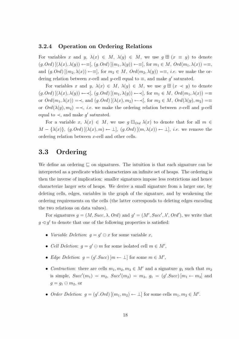
3.2.4 Operation on Ordering Relations

For variables x and y, λ(x) ∈ M , λ(y) ∈ M , we use g � (x ≡ y) to denote

(g.Ord) [(λ(x), λ(y))←≡], (g.Ord) [(m1, λ(y))←≡], for m1 ∈M , Ord(m1, λ(x)) =≡,

and (g.Ord) [(m2, λ(x))←≡], for m2 ∈ M , Ord(m2, λ(y)) =≡, i.e. we make the or-

dering relation between x-cell and y-cell equal to ≡, and make g′ saturated.

For variables x and y, λ(x) ∈ M , λ(y) ∈ M , we use g � (x ≺ y) to denote

(g.Ord) [(λ(x), λ(y))←≺], (g.Ord) [(m1, λ(y))←≺], for m1 ∈ M , Ord(m1, λ(x)) =≡or Ord(m1, λ(x)) =≺, and (g.Ord) [(λ(x),m2)←≺], for m2 ∈ M , Ord(λ(y),m2) =≡or Ord(λ(y),m2) =≺, i.e. we make the ordering relation between x-cell and y-cell

equal to ≺, and make g′ saturated.

For a variable x, λ(x) ∈ M , we use g �Ord λ(x) to denote that for all m ∈M − {λ(x)}, (g.Ord) [(λ(x),m)← ⊥], (g.Ord) [(m,λ(x))← ⊥], i.e. we remove the

ordering relation between x-cell and other cells.

3.3 Ordering

We define an ordering v on signatures. The intuition is that each signature can be

interpreted as a predicate which characterizes an infinite set of heaps. The ordering is

then the inverse of implication: smaller signatures impose less restrictions and hence

characterize larger sets of heaps. We derive a small signature from a larger one, by

deleting cells, edges, variables in the graph of the signature, and by weakening the

ordering requirements on the cells (the latter corresponds to deleting edges encoding

the two relations on data values).

For signatures g = (M, Succ, λ,Ord) and g′ = (M ′, Succ ′, λ′,Ord ′), we write that

g � g′ to denote that one of the following properties is satisfied:

• Variable Deletion: g = g′ x for some variable x,

• Cell Deletion: g = g′ m for some isolated cell m ∈M ′,

• Edge Deletion: g = (g′.Succ) [m← ⊥] for some m ∈M ′,

• Contraction: there are cells m1,m2,m3 ∈ M ′ and a signature g1 such that m2

is simple, Succ ′(m1) = m2, Succ ′(m2) = m3, g1 = (g′.Succ) [m1 ← m3] and

g = g1 m2, or

• Order Deletion: g = (g′.Ord) [(m1,m2)← ⊥] for some cells m1,m2 ∈M ′.

18

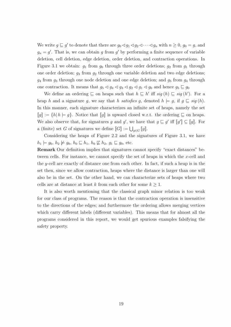
We write g v g′ to denote that there are g0 �g1 �g2 � · · ·�gn with n ≥ 0, g0 = g, and

gn = g′. That is, we can obtain g from g′ by performing a finite sequence of variable

deletion, cell deletion, edge deletion, order deletion, and contraction operations. In

Figure 3.1 we obtain: g1 from g0 through three order deletions; g2 from g1 through

one order deletion; g3 from g2 through one variable deletion and two edge deletions;

g4 from g3 through one node deletion and one edge deletion; and g5 from g4 through

one contraction. It means that g5 � g4 � g3 � g2 � g1 � g0 and hence g5 v g0

We define an ordering v on heaps such that h v h′ iff sig (h) v sig (h′). For a

heap h and a signature g, we say that h satisfies g, denoted h |= g, if g v sig (h).

In this manner, each signature characterizes an infinite set of heaps, namely the set

[[g]] := {h|h |= g}. Notice that [[g]] is upward closed w.r.t. the ordering v on heaps.

We also observe that, for signatures g and g′, we have that g v g′ iff [[g′]] ⊆ [[g]]. For

a (finite) set G of signatures we define [[G]] :=⋃g∈G [[g]].

Considering the heaps of Figure 2.2 and the signatures of Figure 3.1, we have

h1 |= g0, h2 6|= g0, h0 v h1, h0 6v h2, g1 v g0, etc.

Remark Our definition implies that signatures cannot specify “exact distances” be-

tween cells. For instance, we cannot specify the set of heaps in which the x-cell and

the y-cell are exactly of distance one from each other. In fact, if such a heap is in the

set then, since we allow contraction, heaps where the distance is larger than one will

also be in the set. On the other hand, we can characterize sets of heaps where two

cells are at distance at least k from each other for some k ≥ 1.

It is also worth mentioning that the classical graph minor relation is too weak

for our class of programs. The reason is that the contraction operation is insensitive

to the directions of the edges; and furthermore the ordering allows merging vertices

which carry different labels (different variables). This means that for almost all the

programs considered in this report, we would get spurious examples falsifying the

safety property.

19

Chapter 4

Bad Configurations

In this chapter, we show how to use signatures in order to specify sets of bad heaps

for programs which produce sorted single linked lists. In particular, the bad configu-

rations of sorted linear list, sorted cyclic list, sorted partition, inversely sorted linear

list and inversely sorted cyclic list are introduced.

A signature is interpreted as a forbidden pattern which should not occur inside the

heap. Fix a heap h = (M, Succ, λ,Val). A loop in h is a set {m0, . . . ,mn} of cells such

that Succ(mi) = mi+1 for all i : 0 ≤ i < n, and Succ(mn) = m0. For cells m,m′ ∈M ,

we say that m′ is visible from m if there are cells m0,m1, . . . ,mn for some n ≥ 0 such

that m0 = m, mn = m′, and mi+1 = Succ(mi) for all i : 0 ≤ i < n. In other words,

there is a (possibly empty) path in the graph leading from m to m′. We say that m′

is strictly visible from m if n > 0 (i.e. the path is not empty). A set M ′ ⊆ M is said

to be visible from m if some m′ ∈M ′ is visible from m.

4.1 Sorted Linear List

Considering programs such as insert, insertion sort, bubble sort and the merging

procedure of two sorted linear lists, we would like such programs to produce a heap

which is a linear list. Furthermore, the heap should not contain any garbage, and

the output list should be sorted. For each of these three properties, we describe the

corresponding forbidden patterns as a set of signatures which characterize exactly

those heaps which violate the property. Then, we will collect all these signatures into

a single set which characterizes the set of bad configurations.

4.1.1 Well-Formedness

20

x ∗b1: b2: ∗x

xb3: b4: x

We say that h is well-formed w.r.t a variable x if # is visi-

ble form the x-cell. Equivalently, neither the cell ∗ nor any

loop is visible from the x-cell. Intuitively, if a heap satis-

fies this condition, then the part of the heap visible from the x-cell forms a lin-

ear list ending with #. For instance, the heap of Figure 2.1 is well-formed w.r.t.

the variables v and z. In Figure 2.2, h0 is not well-formed w.r.t. the variables x

and z (a loop is visible), and h4 is not well-formed w.r.t. z (the cell ∗ is visi-

ble). The set of heaps violating well-formedness w.r.t. x are characterized by the

four signatures in the figure to the right. The signatures b1 and b2 characterize (to-

gether) all heaps in which the cell ∗ is visible from the x-cell. The signatures b3

and b4 characterize (together) all heaps in which a loop is visible from the x-cell.

4.1.2 Garbage

xb5: b6: x

x#b7: b8: #

x

xb9: ∗ b10: ∗

x

We say that h contains garbage w.r.t a variable x if there is

a cell m ∈ M in h which is not visible from the x-cell. In

Figure 2.2, the heap h0 contains one cell which is garbage

w.r.t. x, namely the cell with value 1. The figure to the right

shows six signatures which together characterize the set of

heaps which contain garbage w.r.t. x.

4.1.3 Sortedness

b11:A heap is said to be sorted if it satisfies the condition that whenever a

cell m1 ∈M is visible from a cell m2 ∈M then Val(m1) ≤ Val(m2).

For instance, in Figure 2.2, only h5 is sorted. The figure to the right shows a signature

which characterizes all heaps which are not sorted.

4.1.4 Putting Everything Together

∗b12: b13:Given a (reference) variable x, a configuration is considered to

be bad w.r.t. x if it violates one of the conditions of being well-

formed w.r.t. x, not containing garbage w.r.t. x, or being sorted. As explained above,

the signatures b1, . . . , b11 characterize the set of heaps which are bad for a sorted

linear list w.r.t. x. We observe that b1 v b9, b2 v b10, b3 v b5 and b4 v b6, which

means that the signatures b5, b6, b9, b10 can be discarded from the set above. Actually,

a configuration is bad if there is a cell with successor ∗ or a loop pattern in the heap,

no matter where x points to. The signature b12 characterizes the cell with successor ∗,

21

while the loop pattern is characterized by signature b13. According to the ordering of

signatures, we have b12 v b1, b13 v b3 and b13 v b4. Then, the signatures b1, b3, b4 are

discarded from the set, while the signatures b12, b13 are added into the set. Therefore,

the set of bad configurations for a sorted linear list w.r.t. x is characterized by the

set {b2, b7, b8, b11, b12, b13}.

4.2 Sorted Cyclic List

Considering program such as cyclic bubble sort, we would like such program to pro-

duce a heap which is a cyclic list. Furthermore, the heap should not contain any

garbage, and the output list should be sorted. Similar to the sorted linear list case,

we describe the forbidden patterns of these three properties and collect all the signa-

tures into a single set which exactly characterizes the set of bad configurations.

4.2.1 Well-Formedness

x ∗b14: b15: ∗xb16: #

x

x#b17:

xb18:

We say that h is cyclically well-formed w.r.t. a variable x if

the x-cell belongs to a loop. Intuitively, if a heap satisfies

this condition, then the part of the heap visible from the

x-cell forms a cyclic list. The set of heaps violating cyclic well-formedness w.r.t. x

are characterized by the five signatures in the figure to the right. The signatures b14

and b15 characterize (together) all heaps in which the cell ∗ is visible from the x-cell,

and the signatures b16 and b17 characterize (together) all heaps in which the cell #

is visible from the x-cell. The signature b18 characterizes all heaps in which a loop is

visible from the x-cell, but where the x-cell itself is not part of the loop.

4.2.2 Garbage

The garbage for a cyclic list is defined exactly the same as the linear list case in

Section 4.3.2, which is characterized by the set of signatures {b5, b6, b7, b8, b9, b10}.

4.2.3 Sortedness

xb19:

xb20:

A heap is said to be cyclically sorted with respect to the variable

x if whenever a cell m ∈M belongs to the same loop as the x-cell,

then either Val(m) ≤ Val(Succ(m)) or Succ(m) = λ(x), but not

both. Intuitively, this means that the x-cell has the smallest value

of all cells in the cycle, and each consecutive pair of cells in the cycle is pairwise

22

sorted. The figure to the right shows two signatures b19 and b20, which characterize

all heaps that are not cyclically sorted w.r.t. x.

4.2.4 Putting Everything Together

∗b21:

#b22:

b23:

As explained above, the signatures b5, . . . , b10, b14, . . . , b20 characterize

the set of heaps which are bad for a sorted cyclic list w.r.t. x. Observe

that b14 v b9, b15 v b10, b16 v b8, b17 v b7 and b18 v b5, which means that

the signatures b5, b7, b8, b9, b10 can be discarded from the set above. Ac-

tually, a configuration is bad if one of the following conditions is satisfied

no matter where x points to: (i) there is a cell with successor ∗, which is character-

ized by signature b21; (ii) there is a cell with successor #, which is characterized by

signature b22; (iii) there is a cell out of the loop, which is characterized by signature

b23. According to the ordering of signatures, we have b21 v b14, b22 v b17, b23 v b6 and

b23 v b18. Then, the signatures b6, b14, b17, b18 are discarded from the set, while the

signatures b21, b22, b23 are added into the set. Therefore, the set of bad configurations

for a sorted cyclic list w.r.t. x is characterized by the set {b15, b16, b19, b20, b21, b22, b23}.

4.3 Sorted Partition

Considering the partition program, we would like such program to produce a heap

which contains two linear lists. Furthermore, the heap should not contain any garbage,

there is no sharing part between these two linear lists and all the elements in one list

are greater than or equal to the first element of the original list, while the elements

in the other list are stictly smaller than that. We describe the forbidden patterns

of these four properties and collect all the signatures into a single set which exactly

characterizes the set of bad configurations.

4.3.1 Well-Formedness

y∗b24: b25: ∗

y

yb26: b27: y

We say that h is well-formed w.r.t variables x and y if # is

visible form both x-cell and y-cell. Equivalently, neither the cell

∗ nor any loop is visible from either x-cell or y-cel. Intuitively,

if a heap satisfies this condition, then the part of the heap visible from the x-cell or

y-cell forms a linear list ending with #. The set of heaps violating well-formedness

w.r.t. x and y are characterized by the set of signatures {b1, . . . , b4, b24, . . . , b27}. The

signatures b1, b2 and b24, b25 characterize (together) all heaps in which the cell ∗ is

23

visible from x-cell and y-cell respectively. The signatures b3, b4 and b26, b27 characterize

(together) all heaps in which a loop is visible from x-cell and y-cell respectively.

4.3.2 Garbage

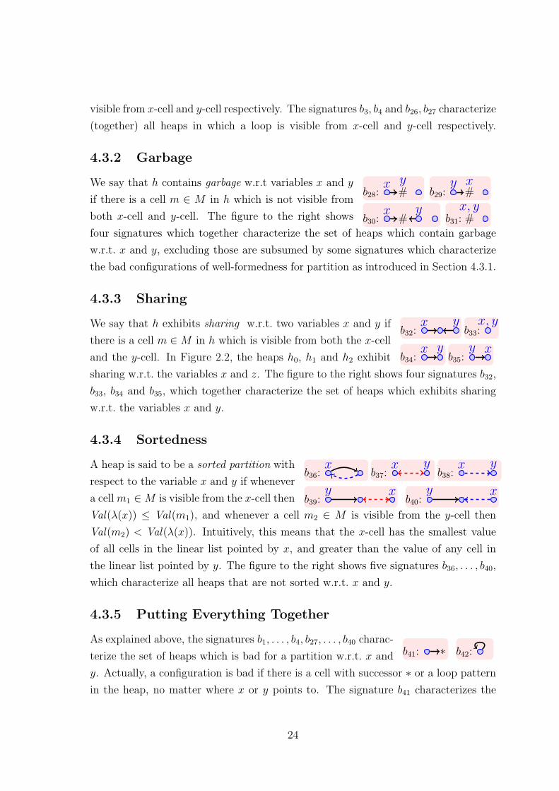
x#y

b28:y

#x

b29:

x#y

b30: b31: #x, y

We say that h contains garbage w.r.t variables x and y

if there is a cell m ∈ M in h which is not visible from

both x-cell and y-cell. The figure to the right shows

four signatures which together characterize the set of heaps which contain garbage

w.r.t. x and y, excluding those are subsumed by some signatures which characterize

the bad configurations of well-formedness for partition as introduced in Section 4.3.1.

4.3.3 Sharing

x yb32: b33:

x, y

x yb34: b35:

y x

We say that h exhibits sharing w.r.t. two variables x and y if

there is a cell m ∈M in h which is visible from both the x-cell

and the y-cell. In Figure 2.2, the heaps h0, h1 and h2 exhibit

sharing w.r.t. the variables x and z. The figure to the right shows four signatures b32,

b33, b34 and b35, which together characterize the set of heaps which exhibits sharing

w.r.t. the variables x and y.

4.3.4 Sortedness

xb36:

x yb37:

x yb38:

y xb39:

y xb40:

A heap is said to be a sorted partition with

respect to the variable x and y if whenever

a cell m1 ∈M is visible from the x-cell then

Val(λ(x)) ≤ Val(m1), and whenever a cell m2 ∈ M is visible from the y-cell then

Val(m2) < Val(λ(x)). Intuitively, this means that the x-cell has the smallest value

of all cells in the linear list pointed by x, and greater than the value of any cell in

the linear list pointed by y. The figure to the right shows five signatures b36, . . . , b40,

which characterize all heaps that are not sorted w.r.t. x and y.

4.3.5 Putting Everything Together

∗b41: b42:As explained above, the signatures b1, . . . , b4, b27, . . . , b40 charac-

terize the set of heaps which is bad for a partition w.r.t. x and

y. Actually, a configuration is bad if there is a cell with successor ∗ or a loop pattern

in the heap, no matter where x or y points to. The signature b41 characterizes the

24

cell with successor ∗, while the loop pattern is characterized by signature b42. Ac-

cording to the ordering of signatures, we have b41 v b1, b41 v b24, b42 v b3, b42 v b26,

b42 v b4 and b42 v b27. Then, the signatures b1, b3, b4, b24, b26, b27 are discarded from

the set, while the signatures b41, b42 are added into the set. Therefore, the set of

bad configurations for a sorted partition w.r.t. x and y is characterized by the set

{b2, b25, b28, . . . , b42}.

4.4 More Bad on Inverse Sortedness

Considering programs such as reversion of a sorted linear list and reversion of a sorted

cyclic list, we would like the output list (linear and cyclic respectively) to be well-

formed, contains no garbage and inversely sorted.

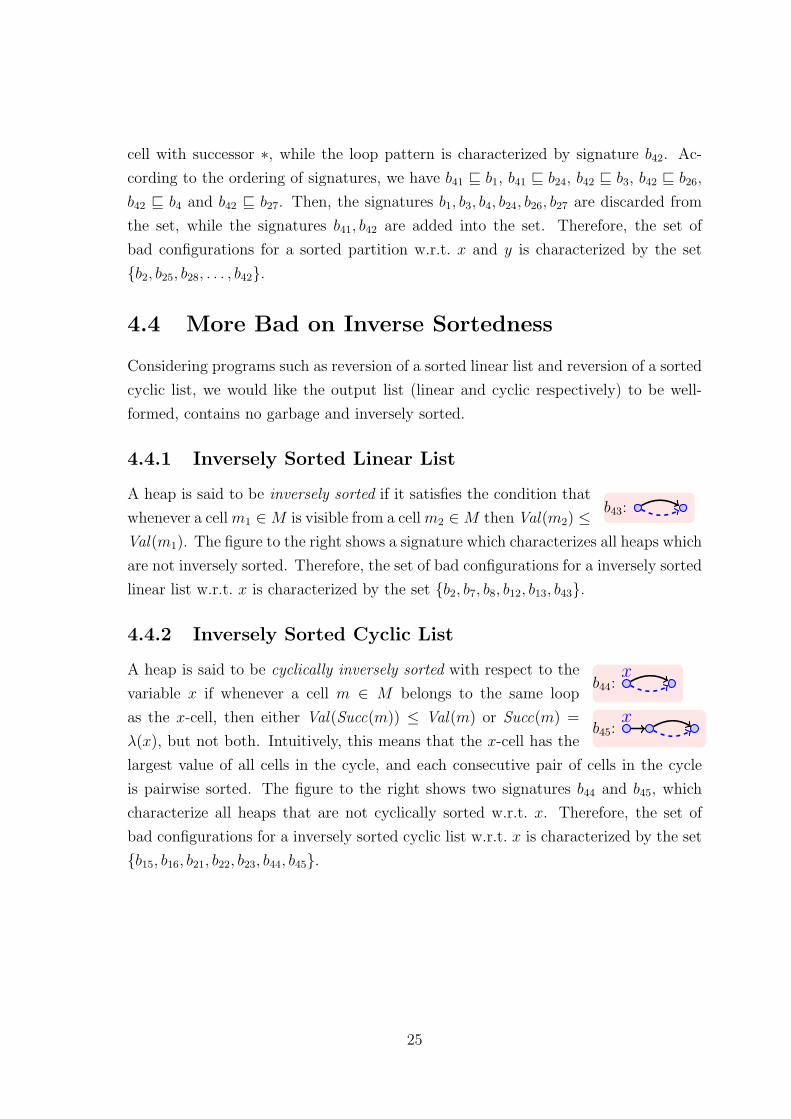
4.4.1 Inversely Sorted Linear List

b43:A heap is said to be inversely sorted if it satisfies the condition that

whenever a cellm1 ∈M is visible from a cellm2 ∈M then Val(m2) ≤Val(m1). The figure to the right shows a signature which characterizes all heaps which

are not inversely sorted. Therefore, the set of bad configurations for a inversely sorted

linear list w.r.t. x is characterized by the set {b2, b7, b8, b12, b13, b43}.

4.4.2 Inversely Sorted Cyclic List

xb44:

xb45:

A heap is said to be cyclically inversely sorted with respect to the

variable x if whenever a cell m ∈ M belongs to the same loop

as the x-cell, then either Val(Succ(m)) ≤ Val(m) or Succ(m) =

λ(x), but not both. Intuitively, this means that the x-cell has the

largest value of all cells in the cycle, and each consecutive pair of cells in the cycle

is pairwise sorted. The figure to the right shows two signatures b44 and b45, which

characterize all heaps that are not cyclically sorted w.r.t. x. Therefore, the set of

bad configurations for a inversely sorted cyclic list w.r.t. x is characterized by the set

{b15, b16, b21, b22, b23, b44, b45}.

25

Chapter 5

Reachability Analysis

In this chapter, we show how to check safety properties through backward reacha-

bility analysis. First, we give an over-approximation −→A of the transition relation

−→. Then, we describe how to compute predecessors of signatures w.r.t. −→A; and

introduce sets of initial heaps (from which the program starts running). Finally, we

describe how to check safety properties using backward reachability analysis.

5.1 Over-Approximation

x, yg:

The basic step in backward reachability analysis is to compute the set of

predecessors of sets of heaps characterized by signatures. More precisely,

for a signature g and an operation op, we would like to compute a finite set G of

signatures such that [[G]] ={h|h op−→ [[g]]

}. Consider the signature g to right. The

set [[g]] contains exactly all heaps where x and y point to the same cell. Consider

the operation op defined by y := z.next . The set H of heaps from which we can

perform the operation and obtain a heap in [[g]] are all those where the x-cell is the

immediate successor of the z-cell. Since signatures cannot capture the immediate

successor relation (see the remark in the end of Chapter 3), the set H cannot be

characterized by any set G of signatures, i.e., there is no G such that [[G]] = H. To

overcome this problem, we define an approximate transition relation −→A which is

an over-approximation of the relation −→. More precisely, for heaps h and h′, we

have hop−→A h

′ iff there is a heap h1 such that h1 v h and h1op−→ h′.

5.2 Computing Predecessors

26

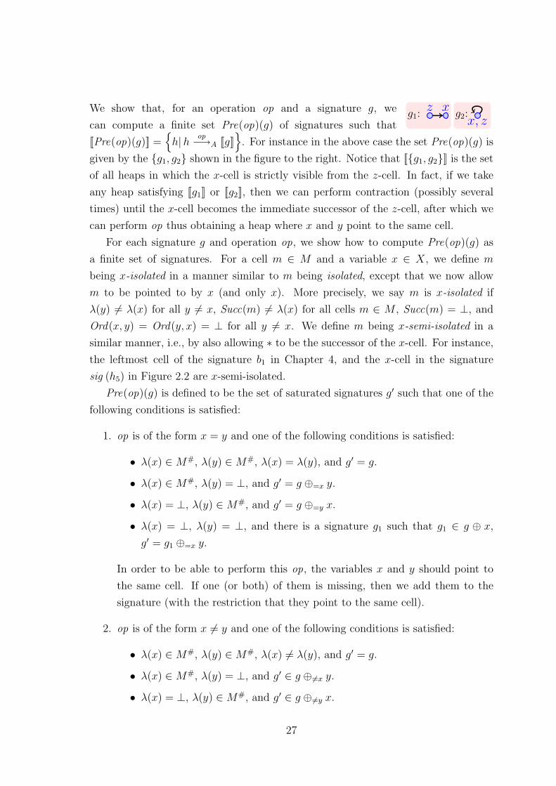
z xg1: g2:x, z

We show that, for an operation op and a signature g, we

can compute a finite set Pre(op)(g) of signatures such that

[[Pre(op)(g)]] ={h|h op−→A [[g]]

}. For instance in the above case the set Pre(op)(g) is

given by the {g1, g2} shown in the figure to the right. Notice that [[{g1, g2}]] is the set

of all heaps in which the x-cell is strictly visible from the z-cell. In fact, if we take

any heap satisfying [[g1]] or [[g2]], then we can perform contraction (possibly several

times) until the x-cell becomes the immediate successor of the z-cell, after which we

can perform op thus obtaining a heap where x and y point to the same cell.

For each signature g and operation op, we show how to compute Pre(op)(g) as

a finite set of signatures. For a cell m ∈ M and a variable x ∈ X, we define m

being x-isolated in a manner similar to m being isolated, except that we now allow

m to be pointed to by x (and only x). More precisely, we say m is x-isolated if

λ(y) 6= λ(x) for all y 6= x, Succ(m) 6= λ(x) for all cells m ∈ M , Succ(m) = ⊥, and

Ord(x, y) = Ord(y, x) = ⊥ for all y 6= x. We define m being x-semi-isolated in a

similar manner, i.e., by also allowing ∗ to be the successor of the x-cell. For instance,

the leftmost cell of the signature b1 in Chapter 4, and the x-cell in the signature

sig (h5) in Figure 2.2 are x-semi-isolated.

Pre(op)(g) is defined to be the set of saturated signatures g′ such that one of the

following conditions is satisfied:

1. op is of the form x = y and one of the following conditions is satisfied:

• λ(x) ∈M#, λ(y) ∈M#, λ(x) = λ(y), and g′ = g.

• λ(x) ∈M#, λ(y) = ⊥, and g′ = g ⊕=x y.

• λ(x) = ⊥, λ(y) ∈M#, and g′ = g ⊕=y x.

• λ(x) = ⊥, λ(y) = ⊥, and there is a signature g1 such that g1 ∈ g ⊕ x,

g′ = g1 ⊕=x y.

In order to be able to perform this op, the variables x and y should point to

the same cell. If one (or both) of them is missing, then we add them to the

signature (with the restriction that they point to the same cell).

2. op is of the form x 6= y and one of the following conditions is satisfied:

• λ(x) ∈M#, λ(y) ∈M#, λ(x) 6= λ(y), and g′ = g.

• λ(x) ∈M#, λ(y) = ⊥, and g′ ∈ g ⊕ 6=x y.

• λ(x) = ⊥, λ(y) ∈M#, and g′ ∈ g ⊕ 6=y x.

27

• λ(x) = ⊥, λ(y) = ⊥, and there is a signature g1 such that g1 ∈ g ⊕ x,

g′ ∈ g1 ⊕6=x y.

We proceed as in case 1, but now under the restriction that x and y point to

different cells (rather than to the same cell).

3. op is of the form x := y and one of the following conditions is satisfied:

• λ(x) ∈M#, λ(y) ∈M#, λ(x) = λ(y), and g′ = g x.

• λ(x) ∈M#, λ(y) = ⊥, and there is a signature g1 such that g1 = g ⊕=x y,

g′ = g1 x.

• λ(x) = ⊥, λ(y) ∈M#, and g′ = g.

• λ(x) = ⊥, λ(y) = ⊥, and g′ ∈ g ⊕ y.

The difference compared to case 1 is that the variable x may have had any value

before performing the assignment. Therefore, we remove x from the signature.

4. op is of the form x := y.next and one of the following conditions is satisfied:

• λ(x) ∈M#, λ(y) ∈M , Succ(λ(y)) = λ(x), and g′ = g x.

• λ(x) ∈ M#, λ(y) ∈ M , Succ(λ(y)) = ⊥, and there is a signature g1 such

that g1 = g � (y → x), g′ = g1 x.

• λ(x) ∈ M#, λ(y) = ⊥, and there are signatures g1, g2 such that g1 ∈g ⊕x← y, g2 = g1 � (y → x), g′ = g2 x.

• λ(x) = ⊥, λ(y) ∈M , Succ(λ(y)) ∈M#, and g′ = g.

• λ(x) = ⊥, λ(y) ∈M , Succ(λ(y)) = ∗, and there is a signature g1 such that

g1 = g ⊕y→∗ x, g′ = g1 x.

• λ(x) = ⊥, λ(y) ∈M , Succ(λ(y)) = ⊥, and g′ ∈ g � (y →).

• λ(x) = ⊥, λ(y) = ⊥, and there are signatures g1, g2, g3 such that g1 ∈ g⊕x,

g2 ∈ g1 ⊕x← y, g3 = g2 � (y → x), g′ = g3 x.

Similarly to case 3 we remove x from the signature. The successor of y-cell

should be defined and point to x-cell. In case the successor is missing, we add

an edge explicitly from the y-cell to x-cell. Furthermore, if x is missing then

the successor of y may point anywhere inside the signature.

5. op is of the form x.next := y and one of the following conditions is satisfied:

28

• λ(x) ∈M , λ(y) ∈M#, Succ(λ(x)) = λ(y), and g′ = g � (x→).

• λ(x) ∈ M , Succ(λ(x)) ∈ M#, λ(y) = ⊥, and there is a signature g1 such

that g1 ∈ g ⊕x→ y, g′ = g1 � (x→).

• λ(x) ∈M , Succ(λ(x)) = ⊥, λ(y) ∈M#, and g′ = g.

• λ(x) ∈M , Succ(λ(x)) = ⊥, λ(y) = ⊥, and g′ ∈ g ⊕ y.

• λ(x) = ⊥, λ(y) ∈ M#, and there is signature g1 such that g1 ∈ g ⊕y← x,

g′ = g1 � (x→).

• λ(x) = ⊥, λ(y) = ⊥, and there are signatures g1, g2 such that g1 ∈ g ⊕ y,

g2 ∈ g1 ⊕y← x, g′ = g2 � (x→).

After performing this op, the successor of the x-cell should be y-cell. Before

performing this op, the successor could have been anywhere inside the signature,

and the corresponding edge is therefore removed.

6. op is of the form new(x) and one of the following conditions is satisfied:

• λ(x) is x-semi-isolated, and there is signature g1 such that g1 = g λ(x)

and g′ = g1 x.

• λ(x) = ⊥ and g′ = g or g′ ∈ g m for some semi-isolated cell m.

After performing this op, a new x-semi-isolated cell is added. So we remove

the cells which are x-semi-isolated or semi-isolated (when x is not shown in the

signature).

7. op is of the form delete(x) and one of the following conditions is satisfied:

• λ(x) = ∗, and there are a signature g1, g2 such that g1 = g x, g2 =

g1 ⊕ λ(x), g′ = g2 � (ML → x).

• λ(x) = ⊥, and there is signatures g1 such that g1 = g ⊕ λ(x), g′ = g1 �

(ML → x).

After performing this op, the predecessor of x-cell should have successor ∗, and

x is on ∗. So we add an x-isolated cell, pick some cells which has successor ∗and make them point to x-cell.

8. op is of the form read(x ) and one of the following conditions is satisfied:

• λ(x) ∈M , and g′ = g �Ord λ(x).

29

• λ(x) = ⊥, and there is a signature g1 such that g1 ∈ g ⊕6=# x, g′ =

g1 �Ord λ(x)

This op reads the value of x-cell, so we remove all the ordering relations of the

x-cell. When x is not shown, we should put it somewhere first.

9. op is of the form x.num = y.num and one of the following conditions is satisfied:

• λ(x) ∈M , λ(y) ∈M , λ(x) ≡ λ(y), and g′ = g.

• λ(x) ∈M , λ(y) ∈M , Ord(x, y) = ⊥, and g′ = g � (x ≡ y).

• λ(x) ∈ M , λ(y) = ⊥, there is signature g1 such that g1 ∈ g ⊕≡x y, g′ =

g1 � (x ≡ y).

• λ(x) = ⊥, λ(y) ∈ M , there is signature g1 such that g1 ∈ g ⊕≡y x, g′ =

g1 � (x ≡ y).

• λ(x) = ⊥, λ(y) = ⊥, there are signatures g1, g2 such that g1 ∈ g ⊕ 6=# y,

g2 ∈ g1 ⊕≡y x, g′ = g2 � (x ≡ y).

This op is enabled when the values of x-cell and y-cell are the same. If one (or

both) of them is missing, then we add them to the signature (with the restriction

that they have possibly the same value).

10. op is of the form x.num < y.num and one of the following conditions is satisfied:

• λ(x) ∈M , λ(y) ∈M , λ(x) ≺ λ(y), and g′ = g.

• λ(x) ∈M , λ(y) ∈M , Ord(x, y) = ⊥, and g′ = g � (x ≺ y).

• λ(x) ∈ M , λ(y) = ⊥, there is a signature g1 such that g1 ∈ g ⊕x≺ y,

g′ = g1 � (x ≺ y).

• λ(x) = ⊥, λ(y) ∈ M , there is signature g1 such that g1 ∈ g ⊕≺y x, g′ =

g1 � (x ≺ y).

• λ(x) = ⊥, λ(y) = ⊥, there are signatures g1, g2 such that g1 ∈ g ⊕ 6=# y,

g2 ∈ g1 ⊕≺y x, g′ = g2 � (x ≺ y).

We proceed as in case 9, but now under the restriction that x-cell has smaller

value than y-cell (rather than to the same value).

11. op is of the form x.num := y.num and one of the following conditions is satisfied:

• λ(x) ∈M , λ(y) ∈M , λ(x) ≡ λ(y), and g′ = g �Ord λ(x).

30

• λ(x) ∈M , λ(y) ∈M , Ord(x, y) = ⊥, and g′ = g �Ord λ(x).

• λ(x) ∈ M , λ(y) = ⊥, and there is a signature g1 such that g1 ∈ g ⊕≡x y,

g′ = g1 �Ord λ(x).

• λ(x) = ⊥, λ(y) ∈M , and g′ = g.

• λ(x) = ⊥, λ(y) = ⊥, and g′ ∈ g ⊕6=# y.

The difference compared to case 9 is that the x-cell may have had any value

before performing the assignment. Therefore, we remove the ordering relation

of x-cell from the signature.

12. op is of the form x.num :< y.num and one of the following conditions is satisfied:

• λ(x) ∈M , λ(y) ∈M , λ(x) ≺ λ(y), and g′ = g �Ord λ(x).

• λ(x) ∈M , λ(y) ∈M , Ord(x, y) = ⊥, and g′ = g �Ord λ(x).

• λ(x) ∈ M , λ(y) = ⊥, and there is a signature g1 such that g1 ∈ g ⊕x≺ y,

g′ = g1 �Ord λ(x).

• λ(x) = ⊥, λ(y) ∈M , and g′ = g.

• λ(x) = ⊥, λ(y) = ⊥, and g′ ∈ g ⊕6=# y.

We proceed as in case 11, but now under the restriction that x-cell has smaller

value than y-cell.

13. op is of the form x.num :> y.num and one of the following conditions is satisfied:

• λ(x) ∈M , λ(y) ∈M , λ(y) ≺ λ(x), and g′ = g �Ord λ(x).

• λ(x) ∈M , λ(y) ∈M , Ord(x, y) = ⊥, and g′ = g �Ord λ(x).

• λ(x) ∈ M , λ(y) = ⊥, and there is a signature g1 such that g1 ∈ g ⊕≺x y,

g′ = g1 �Ord λ(x).

• λ(x) = ⊥, λ(y) ∈M , and g′ = g.

• λ(x) = ⊥, λ(y) = ⊥, and g′ ∈ g ⊕6=# y.

We proceed as in case 11, but now under the restriction that x-cell has bigger

value than y-cell.

31

5.3 Initial Heaps

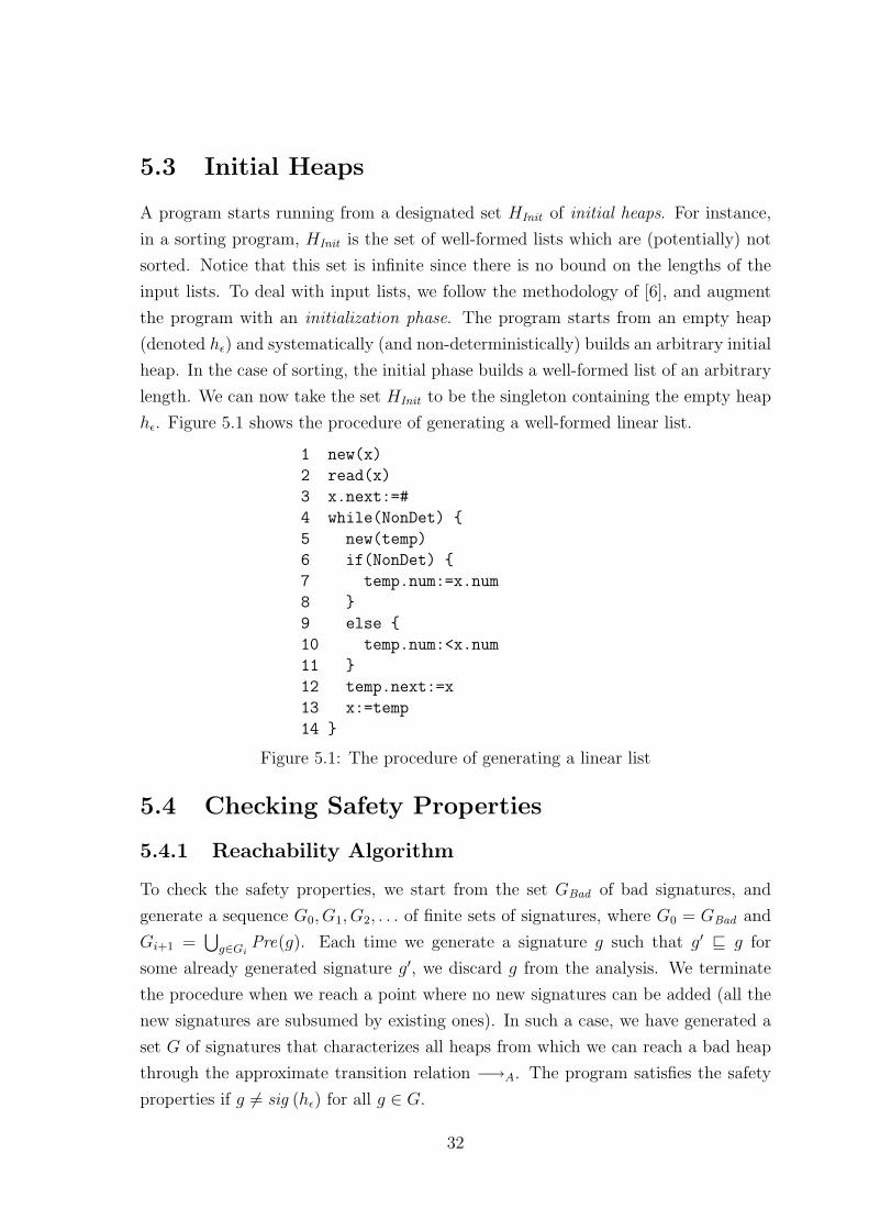
A program starts running from a designated set HInit of initial heaps. For instance,

in a sorting program, HInit is the set of well-formed lists which are (potentially) not

sorted. Notice that this set is infinite since there is no bound on the lengths of the

input lists. To deal with input lists, we follow the methodology of [6], and augment

the program with an initialization phase. The program starts from an empty heap

(denoted hε) and systematically (and non-deterministically) builds an arbitrary initial

heap. In the case of sorting, the initial phase builds a well-formed list of an arbitrary

length. We can now take the set HInit to be the singleton containing the empty heap

hε. Figure 5.1 shows the procedure of generating a well-formed linear list.

1 new(x)

2 read(x)

3 x.next:=#

4 while(NonDet) {

5 new(temp)

6 if(NonDet) {

7 temp.num:=x.num

8 }

9 else {

10 temp.num:<x.num

11 }

12 temp.next:=x

13 x:=temp

14 }

Figure 5.1: The procedure of generating a linear list

5.4 Checking Safety Properties

5.4.1 Reachability Algorithm

To check the safety properties, we start from the set GBad of bad signatures, and

generate a sequence G0, G1, G2, . . . of finite sets of signatures, where G0 = GBad and

Gi+1 =⋃g∈Gi

Pre(g). Each time we generate a signature g such that g′ v g for

some already generated signature g′, we discard g from the analysis. We terminate

the procedure when we reach a point where no new signatures can be added (all the

new signatures are subsumed by existing ones). In such a case, we have generated a

set G of signatures that characterizes all heaps from which we can reach a bad heap

through the approximate transition relation −→A. The program satisfies the safety

properties if g 6= sig (hε) for all g ∈ G.

32

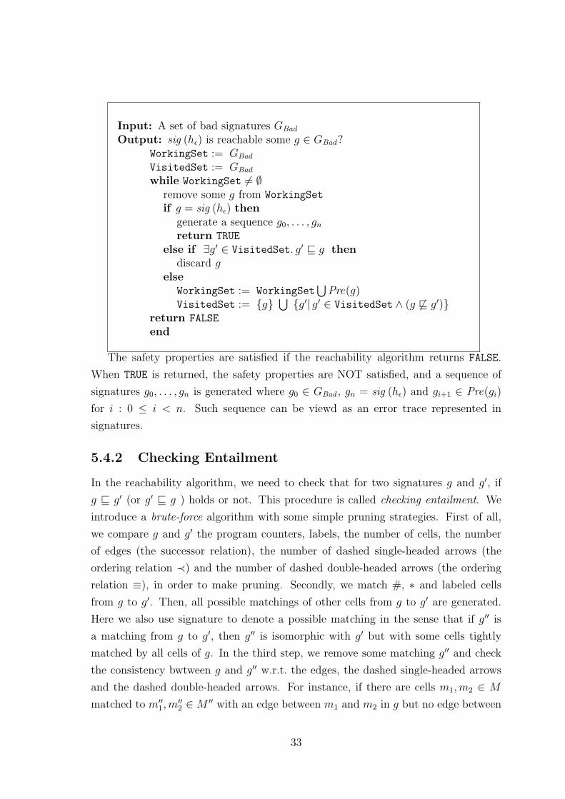
Input: A set of bad signatures GBad

Output: sig (hε) is reachable some g ∈ GBad?WorkingSet := GBad

VisitedSet := GBad

while WorkingSet 6= ∅remove some g from WorkingSet

if g = sig (hε) thengenerate a sequence g0, . . . , gnreturn TRUE

else if ∃g′ ∈ VisitedSet. g′ v g thendiscard g

elseWorkingSet := WorkingSet

⋃Pre(g)

VisitedSet := {g}⋃{g′| g′ ∈ VisitedSet ∧ (g 6v g′)}

return FALSE

end

The safety properties are satisfied if the reachability algorithm returns FALSE.

When TRUE is returned, the safety properties are NOT satisfied, and a sequence of

signatures g0, . . . , gn is generated where g0 ∈ GBad , gn = sig (hε) and gi+1 ∈ Pre(gi)

for i : 0 ≤ i < n. Such sequence can be viewd as an error trace represented in

signatures.

5.4.2 Checking Entailment

In the reachability algorithm, we need to check that for two signatures g and g′, if

g v g′ (or g′ v g ) holds or not. This procedure is called checking entailment. We

introduce a brute-force algorithm with some simple pruning strategies. First of all,

we compare g and g′ the program counters, labels, the number of cells, the number

of edges (the successor relation), the number of dashed single-headed arrows (the

ordering relation ≺) and the number of dashed double-headed arrows (the ordering

relation ≡), in order to make pruning. Secondly, we match #, ∗ and labeled cells

from g to g′. Then, all possible matchings of other cells from g to g′ are generated.

Here we also use signature to denote a possible matching in the sense that if g′′ is

a matching from g to g′, then g′′ is isomorphic with g′ but with some cells tightly

matched by all cells of g. In the third step, we remove some matching g′′ and check

the consistency bwtween g and g′′ w.r.t. the edges, the dashed single-headed arrows

and the dashed double-headed arrows. For instance, if there are cells m1,m2 ∈ M

matched to m′′1,m′′2 ∈M ′′ with an edge between m1 and m2 in g but no edge between

33

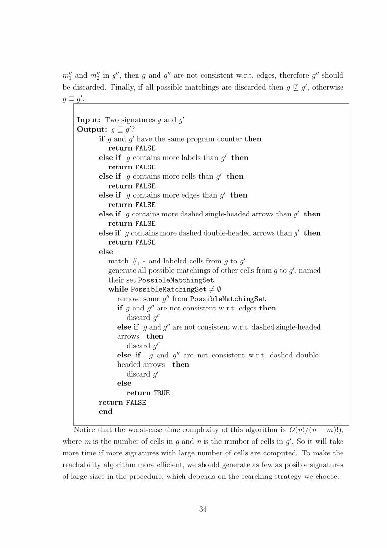
m′′1 and m′′2 in g′′, then g and g′′ are not consistent w.r.t. edges, therefore g′′ should

be discarded. Finally, if all possible matchings are discarded then g 6v g′, otherwise

g v g′.

Input: Two signatures g and g′

Output: g v g′?if g and g′ have the same program counter then

return FALSE

else if g contains more labels than g′ thenreturn FALSE

else if g contains more cells than g′ thenreturn FALSE

else if g contains more edges than g′ thenreturn FALSE

else if g contains more dashed single-headed arrows than g′ thenreturn FALSE

else if g contains more dashed double-headed arrows than g′ thenreturn FALSE

elsematch #, ∗ and labeled cells from g to g′

generate all possible matchings of other cells from g to g′, namedtheir set PossibleMatchingSetwhile PossibleMatchingSet 6= ∅

remove some g′′ from PossibleMatchingSet

if g and g′′ are not consistent w.r.t. edges thendiscard g′′

else if g and g′′ are not consistent w.r.t. dashed single-headedarrows then

discard g′′

else if g and g′′ are not consistent w.r.t. dashed double-headed arrows then

discard g′′

elsereturn TRUE

return FALSE

end

Notice that the worst-case time complexity of this algorithm is O(n!/(n − m)!),

where m is the number of cells in g and n is the number of cells in g′. So it will take

more time if more signatures with large number of cells are computed. To make the

reachability algorithm more efficient, we should generate as few as posible signatures

of large sizes in the procedure, which depends on the searching strategy we choose.

34

5.4.3 Searching Strategies

In the reachability algorithm, we need to remove some g from WorkingSet and com-

pute Pre(g).

A common method is based on the pricinple of breadth-first search. In each it-

eration, we take all signatures in the WorkingSet, compute their predecessors and

put them into a set called NewWorkingSet, then this NewWorkingSet will be the new

WorkingSet for the next iteration. This method is quite straightforward and easy to

implement. However, when the safety properties are not satisfied and an error-trace

is generated, it will take a long time since we compute all the signatures of the same

depth w.r.t. GBad and an error-trace is usually found after performing a number of

Pre operations. Moveover, even if the safety properties are satisfied, we may compute

a lot of predecessors and some of them have large sizes of cells, which also makes the

method time consuming as discussed in Section 5.4.2.

To overcome these, we propose a new method based on the pricinple of depth-

first search. Actually, an error-trace is usually a sequence of signatures in which

every signature consists a small number of cells, which is observed from our exper-

imental tesings. Based on this observation, instead of taking all signatures in the

WorkingSet in each iteration, we take the signatures which have the same smallest

size of cells in the WorkingSet and name the set of them SmallestSizeWorkingSet.

We compute the predecessors of all signatures in the SmallestSizeWorkingSet and

put them into the set NewWorkingSet, then the new WorkingSet for the next iteration

will be NewWorkingSet⋃

(WorkingSet−SmallestSizeWorkingSet). This depth-first

method provides a way to find the error-trace much faster than the breadth-first

method. And because every time just the signatures of smallest size are taken, we get

as few as possible signatures of very large sizes in the procedure, which also makes

this method more efficient.

In the prototype we implemented, the depth-first method is used.

35

Chapter 6

Experimental Results

In this chapter, we give some example programs and show the experimental results.

6.1 Example Programs

6.1.1 Insert

In Figure 6.1, the insert program is illustrated. It inserts the elem-cell into the

sorted linear list pointed to by x, such that the returning linear list is again sorted.

The initialization phase (lines 1 - 16) first creates a non-empty sorted linear list, and

then an additional node to be inserted. The set of bad configurations is described in

Section 4.1.4.

6.1.2 Insert(bug)

The faulty version of the insert program is identical to the one in Figure 6.1, except

that t1:=x.next is substituted for t1:=x on line 22. It is intended to work the same

way as the correct version, but the faulty initialization of t1 makes it fail for the

case of the elem-cell containing a smaller value than any other value in the list. This

program also uses the set of bad configurations described in Section 4.1.4, and we get

an error-trace to the bad state b11 as expected.

6.1.3 Merge

In Figure 6.2, the merge program is shown. It takes as input two sorted lists x and

y, and merges them into one sorted list x. The set of bad configurations is described

in Section 4.1.4.

36

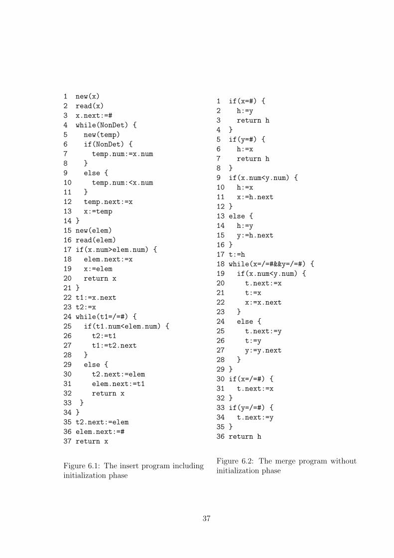
1 new(x)

2 read(x)

3 x.next:=#

4 while(NonDet) {

5 new(temp)

6 if(NonDet) {

7 temp.num:=x.num

8 }

9 else {

10 temp.num:<x.num

11 }

12 temp.next:=x

13 x:=temp

14 }

15 new(elem)

16 read(elem)

17 if(x.num>elem.num) {

18 elem.next:=x

19 x:=elem

20 return x

21 }

22 t1:=x.next

23 t2:=x

24 while(t1=/=#) {

25 if(t1.num<elem.num) {

26 t2:=t1

27 t1:=t2.next

28 }

29 else {

30 t2.next:=elem

31 elem.next:=t1

32 return x

33 }

34 }

35 t2.next:=elem

36 elem.next:=#

37 return x

Figure 6.1: The insert program includinginitialization phase

1 if(x=#) {

2 h:=y

3 return h

4 }

5 if(y=#) {

6 h:=x

7 return h

8 }

9 if(x.num<y.num) {

10 h:=x

11 x:=h.next

12 }

13 else {

14 h:=y

15 y:=h.next

16 }

17 t:=h

18 while(x=/=#&&y=/=#) {

19 if(x.num<y.num) {

20 t.next:=x

21 t:=x

22 x:=x.next

23 }

24 else {

25 t.next:=y

26 t:=y

27 y:=y.next

28 }

29 }

30 if(x=/=#) {

31 t.next:=x

32 }

33 if(y=/=#) {

34 t.next:=y

35 }

36 return h

Figure 6.2: The merge program withoutinitialization phase

37

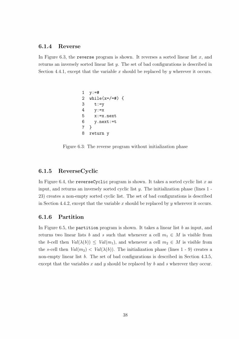
6.1.4 Reverse

In Figure 6.3, the reverse program is shown. It reverses a sorted linear list x, and

returns an inversely sorted linear list y. The set of bad configurations is described in

Section 4.4.1, except that the variable x should be replaced by y wherever it occurs.

1 y:=#

2 while(x=/=#) {

3 t:=y

4 y:=x

5 x:=x.next

6 y.next:=t

7 }

8 return y

Figure 6.3: The reverse program without initialization phase

6.1.5 ReverseCyclic

In Figure 6.4, the reverseCyclic program is shown. It takes a sorted cyclic list x as

input, and returns an inversely sorted cyclic list y. The initialization phase (lines 1 -

23) creates a non-empty sorted cyclic list. The set of bad configurations is described

in Section 4.4.2, except that the variable x should be replaced by y wherever it occurs.

6.1.6 Partition

In Figure 6.5, the partition program is shown. It takes a linear list b as input, and

returns two linear lists b and s such that whenever a cell m1 ∈ M is visible from

the b-cell then Val(λ(b)) ≤ Val(m1), and whenever a cell m2 ∈ M is visible from

the s-cell then Val(m2) < Val(λ(b)). The initialization phase (lines 1 - 9) creates a

non-empty linear list b. The set of bad configurations is described in Section 4.3.5,

except that the variables x and y should be replaced by b and s wherever they occur.

38

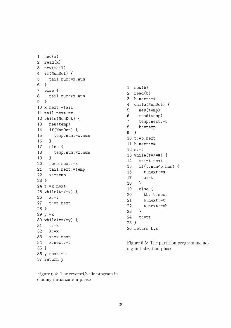
1 new(x)

2 read(x)

3 new(tail)

4 if(NonDet) {

5 tail.num:=x.num

6 }

7 else {

8 tail.num:>x.num

9 }

10 x.next:=tail

11 tail.next:=x

12 while(NonDet) {

13 new(temp)

14 if(NonDet) {

15 temp.num:=x.num

16 }

17 else {

18 temp.num:<x.num

19 }

20 temp.next:=x

21 tail.next:=temp

22 x:=temp

23 }

24 t:=x.next

25 while(t=/=x) {

26 k:=t

27 t:=t.next

28 }

29 y:=k

30 while(x=/=y) {

31 t:=k

32 k:=x

33 x:=x.next

34 k.next:=t

35 }

36 y.next:=k

37 return y

Figure 6.4: The reverseCyclic program in-cluding initialization phase

1 new(b)

2 read(b)

3 b.next:=#

4 while(NonDet) {

5 new(temp)

6 read(temp)

7 temp.next:=b

8 b:=temp

9 }

10 t:=b.next

11 b.next:=#

12 s:=#

13 while(t=/=#) {

14 tt:=t.next

15 if(t.num<b.num) {

16 t.next:=s

17 s:=t

18 }

19 else {

20 tb:=b.next

21 b.next:=t

22 t.next:=tb

23 }

24 t:=tt

25 }

26 return b,s

Figure 6.5: The partition program includ-ing initialization phase

39

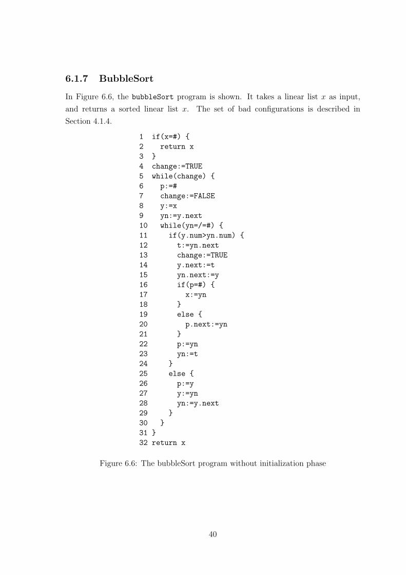
6.1.7 BubbleSort

In Figure 6.6, the bubbleSort program is shown. It takes a linear list x as input,

and returns a sorted linear list x. The set of bad configurations is described in

Section 4.1.4.

1 if(x=#) {

2 return x

3 }

4 change:=TRUE

5 while(change) {

6 p:=#

7 change:=FALSE

8 y:=x

9 yn:=y.next

10 while(yn=/=#) {

11 if(y.num>yn.num) {

12 t:=yn.next

13 change:=TRUE

14 y.next:=t

15 yn.next:=y

16 if(p=#) {

17 x:=yn

18 }

19 else {

20 p.next:=yn

21 }

22 p:=yn

23 yn:=t

24 }

25 else {

26 p:=y

27 y:=yn

28 yn:=y.next

29 }

30 }

31 }

32 return x

Figure 6.6: The bubbleSort program without initialization phase

40

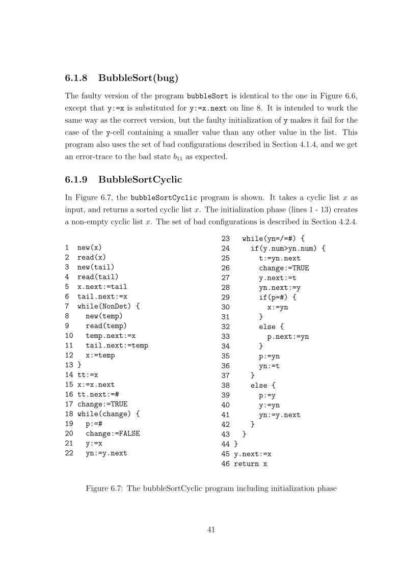
6.1.8 BubbleSort(bug)

The faulty version of the program bubbleSort is identical to the one in Figure 6.6,

except that y:=x is substituted for y:=x.next on line 8. It is intended to work the

same way as the correct version, but the faulty initialization of y makes it fail for the

case of the y-cell containing a smaller value than any other value in the list. This

program also uses the set of bad configurations described in Section 4.1.4, and we get

an error-trace to the bad state b11 as expected.

6.1.9 BubbleSortCyclic

In Figure 6.7, the bubbleSortCyclic program is shown. It takes a cyclic list x as

input, and returns a sorted cyclic list x. The initialization phase (lines 1 - 13) creates

a non-empty cyclic list x. The set of bad configurations is described in Section 4.2.4.

1 new(x)

2 read(x)

3 new(tail)

4 read(tail)

5 x.next:=tail

6 tail.next:=x

7 while(NonDet) {

8 new(temp)

9 read(temp)

10 temp.next:=x

11 tail.next:=temp

12 x:=temp

13 }

14 tt:=x

15 x:=x.next

16 tt.next:=#

17 change:=TRUE

18 while(change) {

19 p:=#

20 change:=FALSE

21 y:=x

22 yn:=y.next

23 while(yn=/=#) {

24 if(y.num>yn.num) {

25 t:=yn.next

26 change:=TRUE

27 y.next:=t

28 yn.next:=y

29 if(p=#) {

30 x:=yn

31 }

32 else {

33 p.next:=yn

34 }

35 p:=yn

36 yn:=t

37 }

38 else {

39 p:=y

40 y:=yn

41 yn:=y.next

42 }

43 }

44 }

45 y.next:=x

46 return x

Figure 6.7: The bubbleSortCyclic program including initialization phase

41

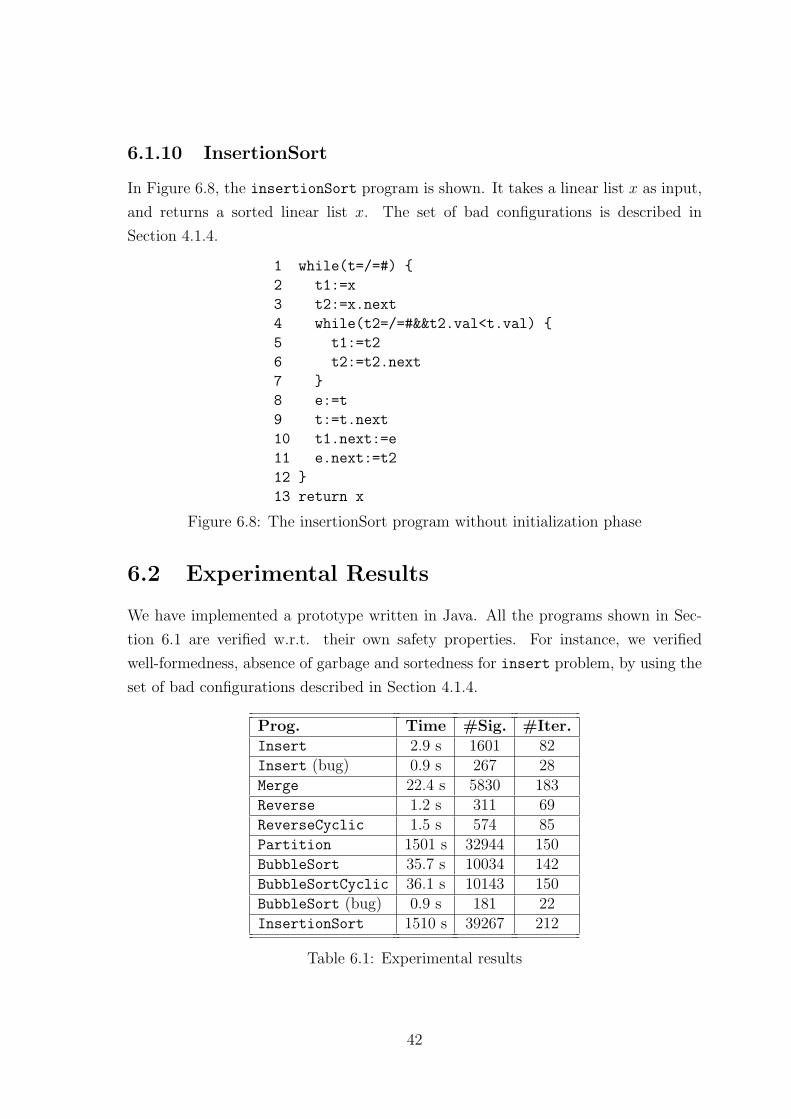
6.1.10 InsertionSort

In Figure 6.8, the insertionSort program is shown. It takes a linear list x as input,

and returns a sorted linear list x. The set of bad configurations is described in

Section 4.1.4.

1 while(t=/=#) {

2 t1:=x

3 t2:=x.next

4 while(t2=/=#&&t2.val<t.val) {

5 t1:=t2

6 t2:=t2.next

7 }

8 e:=t

9 t:=t.next

10 t1.next:=e

11 e.next:=t2

12 }

13 return x

Figure 6.8: The insertionSort program without initialization phase

6.2 Experimental Results

We have implemented a prototype written in Java. All the programs shown in Sec-

tion 6.1 are verified w.r.t. their own safety properties. For instance, we verified

well-formedness, absence of garbage and sortedness for insert problem, by using the

set of bad configurations described in Section 4.1.4.

Prog. Time #Sig. #Iter.Insert 2.9 s 1601 82Insert (bug) 0.9 s 267 28Merge 22.4 s 5830 183Reverse 1.2 s 311 69ReverseCyclic 1.5 s 574 85Partition 1501 s 32944 150BubbleSort 35.7 s 10034 142BubbleSortCyclic 36.1 s 10143 150BubbleSort (bug) 0.9 s 181 22InsertionSort 1510 s 39267 212

Table 6.1: Experimental results

42

Table 6.1 shows the time and number of iterations it took for the run to com-

plete. The column “#Sig.” shows the total number of signatures that were computed

throughout the analysis. All experiments were performed on a 2.2 GHz Intel Core 2

Duo with 4 GB of RAM.

Remark on Spurious Errors Since the transition relation used in the analysis is

an over-approximation, there is a risk of generating false counter-examples. In our

experiments, this arises only in one example, namely a version of Merge (different

from the one included in Table 6.1) in which one pointer x follows another pointer

y, such that there is one cell between x and y. If y moves first followed by x then,

according to our approximation, the pointers may now point to the same cell. This

kind of counter-examples can be dealt with by refining the approximation so that

contraction is allowed only if the size of the resulting list segment will not become

smaller than some given k ≥ 1. For the above counter-example, it is sufficient to take

k = 2. Notice that in the current approximation we have k = 1.

43

Chapter 7

Conclusions and Future Work

We have presented a method for automatic verification of safety properties for pro-

grams which manipulate heaps containing data. The main ingredient is a compact

data structure, called a signature, for symbolic representation of infinite sets of heaps.

Signatures are used as forbidden patterns which characterize heaps violating safety

properties such as absence of garbage, well-formedness, and sortedness. A given safety

property can be checked by performing backward reachability analysis on the set of

signatures. Although the procedure is not guaranteed to terminate in general, our

prototype implementation terminates on all the given examples. The experimental

results are quite encouraging, especially considering the fact that our code is still

highly unoptimized. For instance, most of the verification time is spent on check-

ing entailment between signatures. We are currently using a simple but inefficient

(brute-force) algorithm for checking entailment. We believe that adapting specialized

algorithms such as the one described in [17] will substantially improve performances

of the tool.

Several extensions of our framework can be carried out by refining the considered

preorder (and the abstraction it induces). For instance, it could be possible to consider

integer program variables whose values are related to the lengths of paths in the

heap. Such an extension with arithmetical reasoning can be done in our framework

by considering preorders involving for instance gap-order constraints [14]. Another

direction for future work is to consider more general classes of heaps with multiple

selectors, and then study programs operating on data structures such as doubly-linked

lists and trees both with and without data.

44

Bibliography

[1] P. A. Abdulla, A. Annichini, and A. Bouajjani. Using forward reachability anal-

ysis for verification of lossy channel systems. Formal Methods in System Design,

25(1):39–65, 2004.

[2] P. A. Abdulla, A. Bouajjani, J. Cederberg, F. Haziza, and A. Rezine. Monotonic

abstraction for programs with dynamic memory heaps. In Proc. CAV ’08, volume

5123 of LNCS, pages 341–354, 2008.

[3] P. A. Abdulla, N. B. Henda, G. Delzanno, and A. Rezine. Regular model checking

without transducers. In Proc. TACAS ’07, volume 4424 of LNCS, pages 721–736.

Springer Verlag, 2007.

[4] A. Bouajjani, M. Bozga, P. Habermehl, R. Iosif, P. Moro, and T. Vojnar. Pro-

grams with lists are counter automata. In Proc. CAV ’06, volume 4144 of LNCS,

pages 517–531, 2006.

[5] A. Bouajjani, P. Habermehl, P. Moro, and T. Vojnar. Verifying programs with

dynamic 1-selector-linked structures in regular model checking. In Proc. TACAS

’05, volume 3440 of LNCS, pages 13–29. Springer, 2005.

[6] A. Bouajjani, P. Habermehl, A. Rogalewicz, and T. Vojnar. Abstract tree regular

model checking of complex dynamic data structures. In Proc. SAS ’06, volume

4134 of LNCS, 2006.

[7] A. Bouajjani, P. Habermehl, and T. Vojnar. Abstract regular model checking.

In Proc. CAV ’04, volume 3114 of LNCS, pages 372–386, Boston, 2004.

[8] P. Ganty, J. Raskin, and L. V. Begin. A complete abstract interpretation frame-

work for coverability properties of wsts. In Proc. VMCAI ’06, volume 3855 of

LNCS, pages 49–64, 2006.

45

[9] B. Guo, N. Vachharajani, and D. I. August. Shape analysis with inductive

recursion synthesis. In Proc. PLDI ’07, volume 42, pages 256–265, 2007.

[10] J. Henriksen, J. Jensen, M. Jørgensen, N. Klarlund, B. Paige, T. Rauhe, and

A. Sandholm. Mona: Monadic second-order logic in practice. In Proc. TACAS

’95, volume 1019 of LNCS, 1996.

[11] T. Lev-Ami, T. W. Reps, S. Sagiv, and R. Wilhelm. Putting static analysis

to work for verification: A case study. In Proc. ISSTA ’00, ACM SIGSOFT

International Symposium on Software Testing and Analysis, pages 26–38, 2000.

[12] A. Møller and M. I. Schwartzbach. The pointer assertion logic engine. In Proc.

PLDI ’01, volume 26, pages 221–231, 2001.

[13] H. H. Nguyen, C. David, S. Qin, and W.-N. Chin. Automated verification of

shape and size properties via separation logic. In Proc. VMCAI ’07, volume

4349 of LNCS, pages 251–266, 2007.

[14] P. Revesz. Introduction to Constraint Databases. Springer, 2002.

[15] J. C. Reynolds. Separation logic: A logic for shared mutable data structures. In

Proc. LICS ’02, pages 55–74, 2002.

[16] S. Sagiv, T. Reps, and R. Wilhelm. Parametric shape analysis via 3-valued logic.

ACM Trans. on Programming Languages and Systems, 24(3):217–298, 2002.

[17] G. Valiente. Constrained tree inclusion. J. Discrete Algorithms, 3(2-4):431–447,

2005.

[18] H. Yang, O. Lee, J. Berdine, C. Calcagno, B. Cook, D. Distefano, and P. W.

O’Hearn. Scalable shape analysis for systems code. In Proc. CAV ’08, volume

5123 of LNCS, pages 385–398, 2008.

46