Automating the Simplification of Mathematical Expressions Albert D. Rich, Hawaii

The following commentary refers to the slides at the end of this document.

What�s Really Under the Hood of your CAS? It is perfectly possible to drive a car with little or no understanding of what�s under the hood. That is until the car breaks down late at night, on a lonely stretch of road, �

Similarly, just about everyone who has used a computer algebra system to teach or do mathematics has, on occasion, been surprised and frustrated at the �simplified� results returned by the system. For this reason it is important to have a basic understanding of what is under the hood of your CAS. Such knowledge makes it easier to obtain the results you want, and to avoid those you don�t.

As one of the authors of Derive® and its predecessor, muMATH�, I would like to pass on some of the insights I have gained over the last 25 years implementing these computer algebra systems. I will discuss the principles and methodologies Derive uses to automate the simplification of mathematical expressions.

I begin by summarizing at the overall design of Derive.

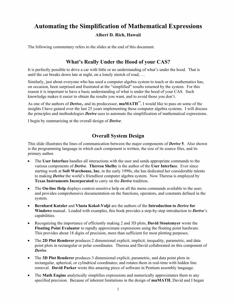
Overall System Design This slide illustrates the lines of communication between the major components of Derive 5. Also shown is the programming language in which each component is written, the size of its source files, and its primary author.

• The User Interface handles all interactions with the user and sends appropriate commands to the various components of Derive. Theresa Shelby is the author of the User Interface. Ever since starting work at Soft Warehouse, Inc. in the early 1990s, she has dedicated her considerable talents to making Derive the world�s friendliest computer algebra system. Now Theresa is employed by Texas Instruments Incorporated to carry on the Derive tradition.

• The On-line Help displays context-sensitive help on all the menu commands available to the user; and provides comprehensive documentation on the functions, operators, and constants defined in the system.

• Bernhard Kutzler and Vlasta Kokol-Voljè are the authors of the Introduction to Derive for Windows manual. Loaded with examples, this book provides a step-by-step introduction to Derive�s capabilities.

• Recognizing the importance of efficiently making 2 and 3D plots, David Stoutemyer wrote the Floating Point Evaluator to rapidly approximate expressions using the floating point hardware. This provides about 18 digits of precision, more than sufficient for most plotting purposes.

• The 2D Plot Renderer produces 2 dimensional explicit, implicit, inequality, parametric, and data point plots in rectangular or polar coordinates. Theresa and David collaborated on this component of Derive.

• The 3D Plot Renderer produces 3 dimensional explicit, parametric, and data point plots in rectangular, spherical, or cylindrical coordinates; and rotates them in real-time with hidden line removal. David Parker wrote this amazing piece of software in Pentium assembly language.

• The Math Engine analytically simplifies expressions and numerically approximates them to any specified precision. Because of inherent limitations in the design of muMATH, David and I began

1

writing a math engine in the mid 1980s using a radical new recursive representation for mathematical expressions, that is both compact and efficient. The Engine is written in the muLISP programming language.

• In the late 1970s, I wrote the first version of muLISP for the Intel 8080 microprocessor with its 64 kilobytes of memory. Since then muLISP has evolved into a general purpose pseudo-code LISP interpreter that takes advantage of the Pentium�s 4 gigabyte address space. Specially adapted for computer algebra, it provides over 500 functions efficiently defined in assembly language, including ones for exact, and high precision approximate, rational arithmetic.

Each one of these components could easily be the basis for a talk itself. But in the interest of time, I will concentrate on how the Math Engine simplifies mathematical expressions.

Expression Processing This blow-up of the Math Engine illustrates how its three components process an expression sent by the User Interface.

First, the Parser converts the expression into a form suitable for use by the Simplifier. Next, the Simplifier transforms the expression into a simpler equivalent, if possible. Finally, the Formatter converts the simplified result into a form suitable for sending back to the User Interface.

Before going into more detail on how the Simplifier works, I will briefly summarize the function of the Parser and Formatter.

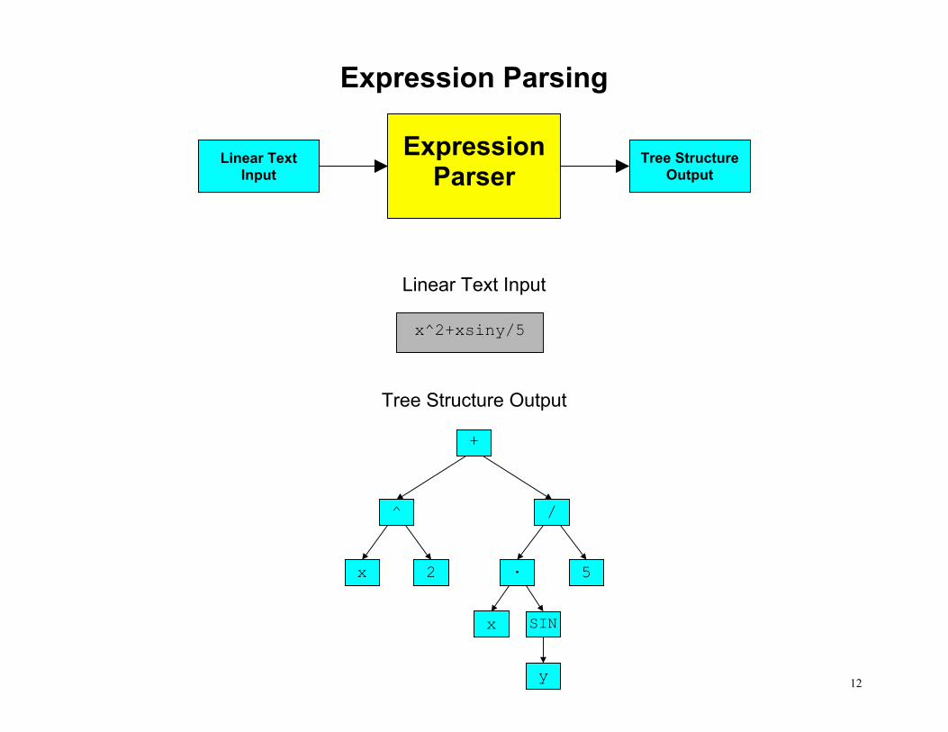
Expression Parsing In Derive, mathematical expressions are entered by typing a line of text on the expression entry line. Parsing is the process of converting this linear input into a tree structure, exactly corresponding to the underlying structure of the mathematical expression.

For example, consider this linear string of characters and its corresponding tree structure. Given a pointer to the tree, it is easy for the Simplifier to determine that the expression is a sum whose first term is raised to the 2nd power, and whose second term is a quotient, etc.

A distinguishing characteristic of Derive�s Parser is its high degree of tolerance for the shortcuts the user can take advantage of while entering expressions. As in this example, an asterisk is not required between �x� and �sin� to indicate multiplication. Also, parentheses are not required following �sin� since its argument is a variable.

Expression Formatting As you might expect, formatting is the converse of parsing mathematical expressions. Thus given a tree structure, the Formatter converts it into lines of text. Multiple lines are returned so the User Interface can display the expression in 2 dimensions, greatly improving the readability of complicated expressions. Here, raised exponents and built-up fractions make clear the underlying structure of the expression.

However, if you intended to enter this expression, it is immediately obvious that a mistake was made. You need parentheses around the desired argument of the sine function.

Parsing and formatting are fascinating subjects in themselves, but that is not the subject of this paper. Instead I will focus in on simplification.

You may be wondering why I am restricting my talk to the simplification of mathematical expressions. After all, Derive can factor polynomials, solve equations, integrate and differentiate expressions, invert

2

matrices, etc. So before I go on, let me explain why all these operations can be regarded as a form of simplification.

Integrating an Expression Consider the process of how you integrate an expression in Derive using a specific example:

• First you enter and highlight the integrand.

• Next you click on the Integrate button and this dialog box is displayed.

• Then you enter the integration variable and the limits of integration.

• Finally you click on the Simplify button and this closed-form result is displayed.

By the way, if your favorite computer algebra system is not Derive, you might try evaluating this definite integral on the competition. In 2001, Vladimir Bondarenko at Simferopol State University in the Ukraine contributed the elegant rule that enables Derive to integrate the reciprocal of any binomial from 0 to infinity.

Integration vs. Simplification The interaction cycle on the previous slide might lead you to think that the User Interface sends an Integrate command to the Math Engine along with the integrand, integration variable, and the limits of integration, as depicted in the top diagram of this slide.

However, what actually happens is that the Interface combines the integrand, the integration variable, and the limits of integration into a single expression using the INT function. Then the Math Engine simplifies this definite integral to the desired closed-form value.

Therefore, the bottom diagram is a more accurate depiction of how Derive simplifies definite integrals to find their value.

Examples of Simplification Here are some other operations Derive does:

• expand factorials

• approximate irrational expressions to any desired precision

• factor polynomials

• differentiate arbitrary functions

• find antiderivatives

• solve equations

Note that all these operations are treated as simplification problems by the Math Engine. Therefore simplification includes virtually all the mathematically interesting things that Derive does. Thus the scope of my talk may not be as limited as you might have thought.

So that brings us to the question: Just what is simplification?

As the relative size of the boxes in these examples illustrate , the primary goal of simplification is not the most compact representation of an expression.

3

Simplification Process To answer the question, you need to know that Derive does simplification in two distinct phases:

First the Reduction Phase recursively reduces expressions to their most elemental form using the lowest level function and operators possible. This reduction maximizes opportunities for cancellations and collections of similar terms and factors to occur. However, the result is often huge and difficult to comprehend.

Therefore, the Restoration Phase restores reduced expressions using higher level functions and operators. This results in a more compact and comprehensible form to humans. But, the transformations done during restoration are just cosmetic, and no additional mathematically significant cancellations will occur.

To make all this more concrete, I will give several examples showing the steps Derive uses to simplify some mathematical expressions.

Simplification of a Trigonometric Expression First consider the simplification of this trigonometric expression at the top of the slide.

• First reduction transformations are applied that replace the secant, tangent, and cotangent functions with equivalent expressions using sines and cosines.

• Next the product of these two sums is expanded.

• Next the last three terms of the sum are placed over a common denominator.

• Then the well known identity for sine squared plus cosine squared results in a significant simplification.

• Finally these transformations restore the tangent and secant functions to produce a slightly more compact result.

Clearly most of the �work� involved in simplification is done during the reduction phase. The restoration phase transformations merely tidy up the result.

Note that Derive uses the same sorts of rules humans do to simplify expressions. There is nothing magical about what Derive can and can�t do.

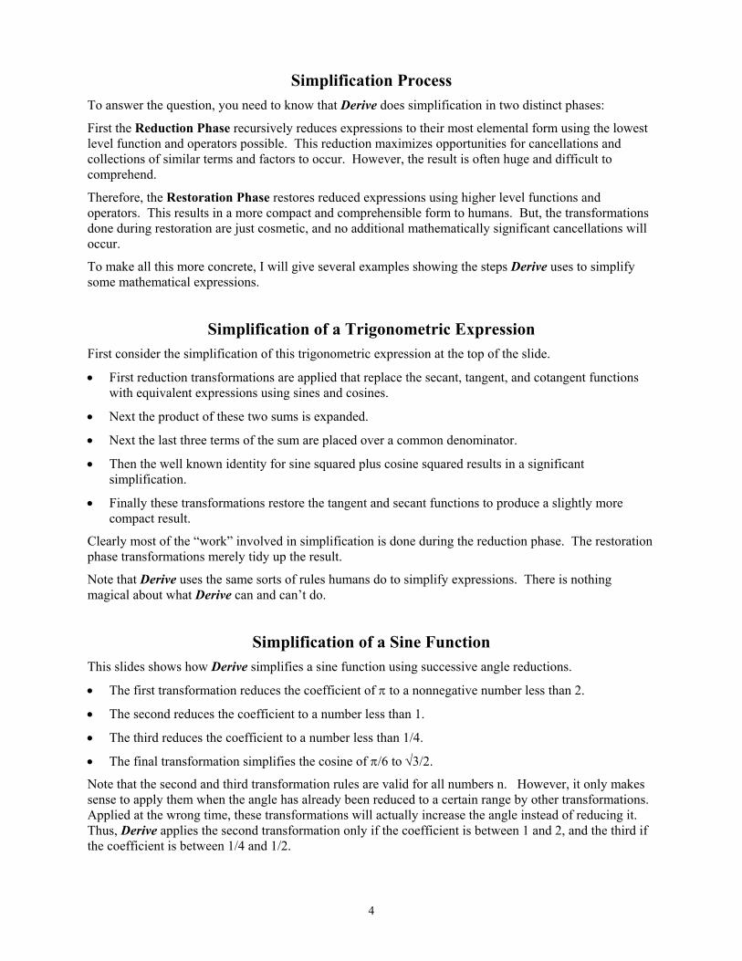
Simplification of a Sine Function This slides shows how Derive simplifies a sine function using successive angle reductions.

• The first transformation reduces the coefficient of π to a nonnegative number less than 2.

• The second reduces the coefficient to a number less than 1.

• The third reduces the coefficient to a number less than 1/4.

• The final transformation simplifies the cosine of π/6 to √3/2.

Note that the second and third transformation rules are valid for all numbers n. However, it only makes sense to apply them when the angle has already been reduced to a certain range by other transformations. Applied at the wrong time, these transformations will actually increase the angle instead of reducing it. Thus, Derive applies the second transformation only if the coefficient is between 1 and 2, and the third if the coefficient is between 1/4 and 1/2.

4

In general, when implementing a computer algebra system, knowing when to apply a rule is as important as knowing the rule itself. If transformation rules are applied indiscriminately, infinite recursion will exhaust memory due to a stack overflow.

Simplification of a Derivative This slides shows how Derive simplifies a derivative involving log and trig functions.

• The first transformation is the rule for the derivative of a quotient;

• The second is for the derivative of a logarithm;

• The third is for the derivative of a power; and

• The fourth is for the derivative of a sine.

• The final transformation cancels sine x squared from the numerator and denominator of the quotient, giving a more compact result.

However, this fortuitous cancellation results in a loss of information that makes integrating this derivative something of a challenge. So, I will show how Derive does it.

Simplification of an Integral This slides shows how Derive simplifies an integral involving log and trig functions.

• The first rule transforms the integral of a difference into the difference of integrals.

• The second rule uses integration by parts to integrate this product .

• The next rule integrates the sine of an expression raised to any power times the cosine of the same expression.

• The next rule differentiates the derivative introduced by integration by parts.

• Here the common factors in the numerator and denominator are cancelled.

• Finally the remaining integrals conveniently cancel each other out, leaving a closed-form result identical to the original expression in the previous slide.

Note that near the beginning of this process, you have the difference of two integrals neither of which has a closed-form antiderivative. Instead of giving up, Derive reduces such integrals to their simplest form so exact cancellations can occur as they do here. Also, this reduction makes it easier to numerically approximate definite integrals using quadrature. This strategy is used throughout Derive�s integrator.

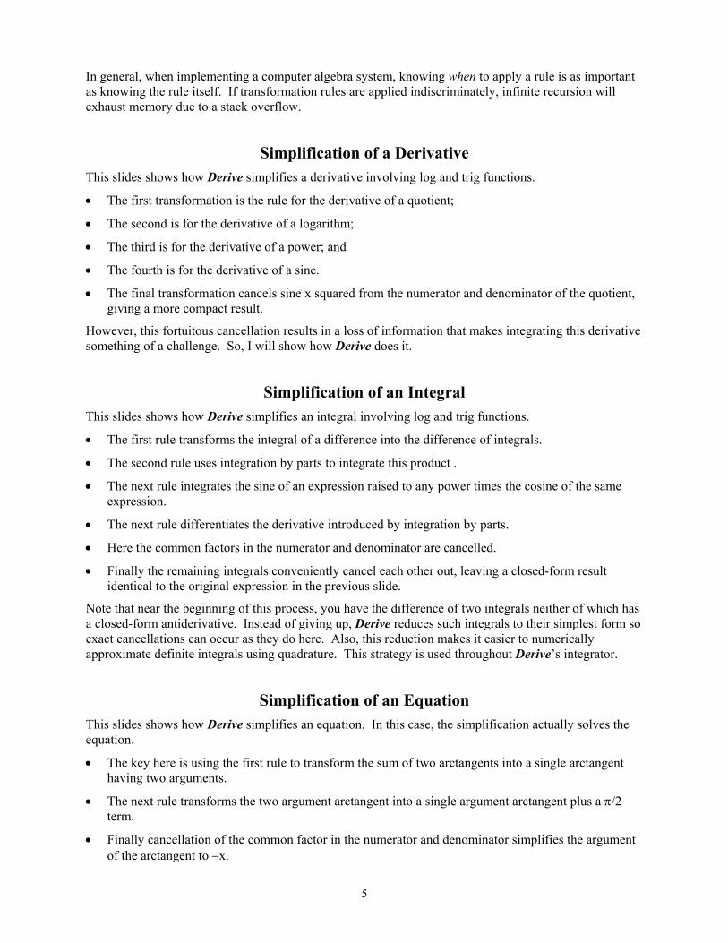
Simplification of an Equation This slides shows how Derive simplifies an equation. In this case, the simplification actually solves the equation.

• The key here is using the first rule to transform the sum of two arctangents into a single arctangent having two arguments.

• The next rule transforms the two argument arctangent into a single argument arctangent plus a π/2 term.

• Finally cancellation of the common factor in the numerator and denominator simplifies the argument of the arctangent to −x.

5

In the course of finding interesting examples for this paper, I derived this formulation of the rule for the sum of two arctangents. It is valid for all real x and y. The other formulations I have seen in Abromowitz & Stegun, and elsewhere, impose restrictions on the domain of x and y that make it difficult to apply the transformation in this example.

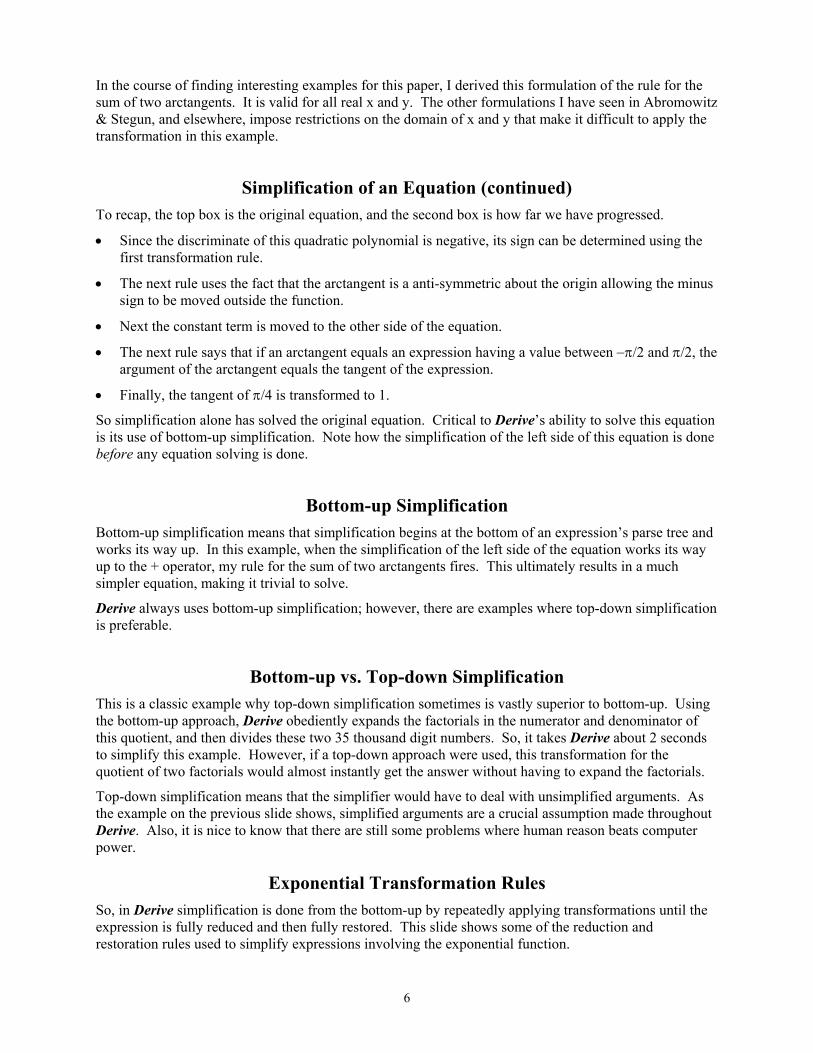
Simplification of an Equation (continued) To recap, the top box is the original equation, and the second box is how far we have progressed.

• Since the discriminate of this quadratic polynomial is negative, its sign can be determined using the first transformation rule.

• The next rule uses the fact that the arctangent is a anti-symmetric about the origin allowing the minus sign to be moved outside the function.

• Next the constant term is moved to the other side of the equation.

• The next rule says that if an arctangent equals an expression having a value between −π/2 and π/2, the argument of the arctangent equals the tangent of the expression.

• Finally, the tangent of π/4 is transformed to 1.

So simplification alone has solved the original equation. Critical to Derive�s ability to solve this equation is its use of bottom-up simplification. Note how the simplification of the left side of this equation is done before any equation solving is done.

Bottom-up Simplification Bottom-up simplification means that simplification begins at the bottom of an expression�s parse tree and works its way up. In this example, when the simplification of the left side of the equation works its way up to the + operator, my rule for the sum of two arctangents fires. This ultimately results in a much simpler equation, making it trivial to solve.

Derive always uses bottom-up simplification; however, there are examples where top-down simplification is preferable.

Bottom-up vs. Top-down Simplification This is a classic example why top-down simplification sometimes is vastly superior to bottom-up. Using the bottom-up approach, Derive obediently expands the factorials in the numerator and denominator of this quotient, and then divides these two 35 thousand digit numbers. So, it takes Derive about 2 seconds to simplify this example. However, if a top-down approach were used, this transformation for the quotient of two factorials would almost instantly get the answer without having to expand the factorials.

Top-down simplification means that the simplifier would have to deal with unsimplified arguments. As the example on the previous slide shows, simplified arguments are a crucial assumption made throughout Derive. Also, it is nice to know that there are still some problems where human reason beats computer power.

Exponential Transformation Rules So, in Derive simplification is done from the bottom-up by repeatedly applying transformations until the expression is fully reduced and then fully restored. This slide shows some of the reduction and restoration rules used to simplify expressions involving the exponential function.

6

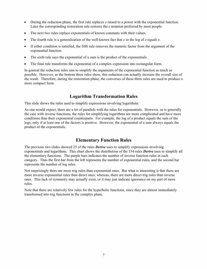
• During the reduction phase, the first rule replaces e raised to a power with the exponential function. Later the corresponding restoration rule restores the e notation preferred by most people.

• The next two rules replace exponentials of known constants with their values.

• The fourth rule is a generalization of the well-known fact that e to the log of z equals z.

• If either condition is satisfied, the fifth rule removes the numeric factor from the argument of the exponential function.

• The sixth rule says the exponential of a sum is the product of the exponentials.

• The final rule transforms the exponential of a complex expression into rectangular form.

In general the reduction rules aim to simplify the arguments of the exponential function as much as possible. However, as the bottom three rules show, this reduction can actually increase the overall size of the result. Therefore, during the restoration phase, the converses of these three rules are used to produce a more compact form.

Logarithm Transformation Rules This slide shows the rules used to simplify expressions involving logarithms.

As one would expect, there are a lot of parallels with the rules for exponentials. However, as is generally the case with inverse functions, the rules for simplifying logarithms are more complicated and have more conditions than their exponential counterparts. For example, the log of a product equals the sum of the logs, only if at least one of the factors is positive. However, the exponential of a sum always equals the product of the exponentials.

Elementary Function Rules The previous two slides showed 25 of the rules Derive uses to simplify expressions involving exponentials and logarithms. This chart shows the distribution of the 334 rules Derive uses to simplify all the elementary functions. The purple bars indicates the number of inverse function rules in each category. Thus the first bar from the left represents the number of exponential rules, and the second bar represents the number of log rules.

Not surprisingly there are more trig rules than exponential ones. But what is interesting is that there are more inverse exponential rules than direct ones; whereas, there are more direct trig rules than inverse ones. This lack of symmetry may actually exist, or it may just indicate ignorance on my part of more rules.

Note that there are relatively few rules for the hyperbolic functions, since they are almost immediately transformed into trig functions in the complex plane.

7

Transformation Rules Moving up a level, this chart summarizes the distribution of the 1380 rules Derive uses to simplify the various categories of mathematical functions and the logical operators. The elementary operators were omitted because their ubiquity makes them difficult to count. Also not counted were the rules for the vector, matrix, and set functions and operators.

I would guess that there are well over 2000 rules in Derive. However, let me caution against using a raw rule count to evaluate the �intelligence� of any computer algebra system.

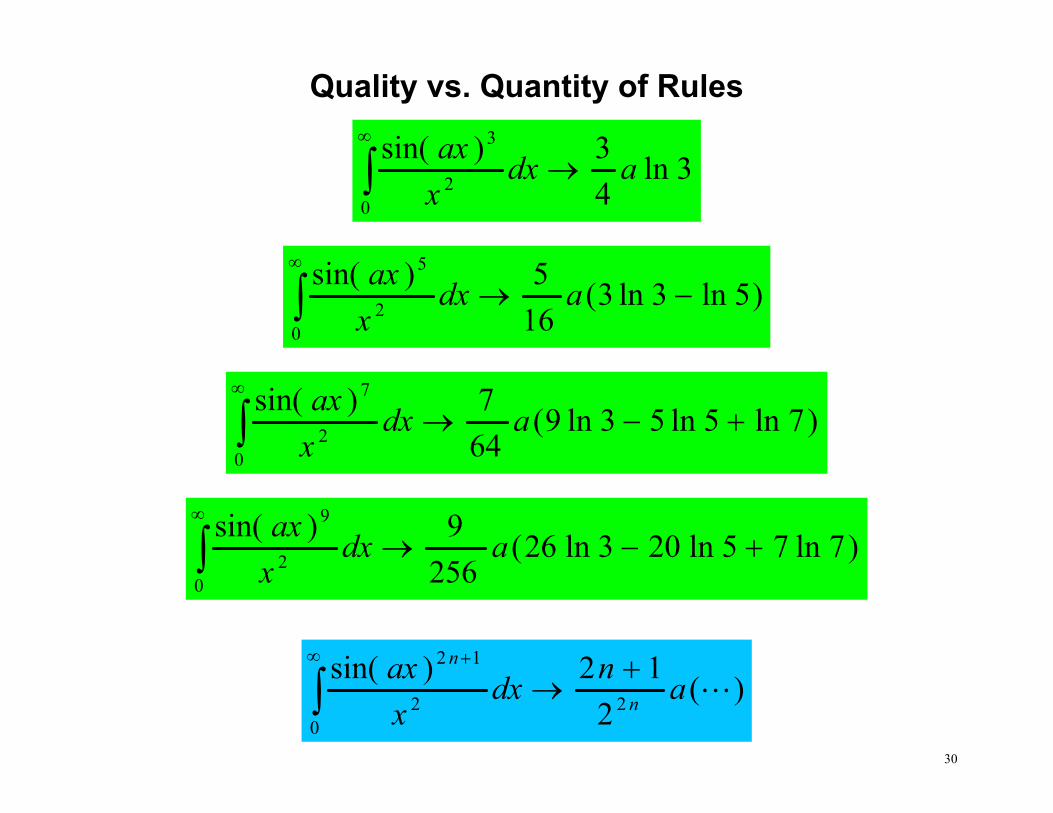
Quality vs. Quantity of Rules Currently Derive uses these rules to simplify the first four integrals of this family. It seemed to me during the writing of this talk that there should exist a single rule that can simplify any member of the family. Using Sloane and Plouffe�s Encyclopedia of Integer Sequences on the coefficients of the log terms, I was able to deduce just such a rule.

So when I replace the four existing rules with this new rule, it will extend the class of definite integrals Derive can find and reduce the rule count by 3. Therefore, when comparing computer algebra systems, the quality of rules is at least as important as the quantity. Also, as stated earlier, now matter how many rules a system has, knowing when to apply them is as important as knowing the rule itself.

In Summary • Simplification includes virtually all the mathematically interesting things Derive does.

• Simplification is done in two distinct phases: Reduction then Restoration.

• A transformation rule should be applied only if it results in a simpler expression.

• There is a trade-off between bottom-up and top-down simplification. Derive does the former.

• Derive employs over 2000 mathematical factoids called transformation rules to simplify expressions.

• The quality of rules in a computer algebra system is at least as important as the quantity.

8

What�s Really Under the Hood of your CAS?

Automating the Simplification of Mathematical Expressions

Albert D. Rich Free-lance Applied Logician Kawaihae, Big Island, Hawaii

9

Overall System Design

10

User Interface Visual C++

1.8 megabytes Theresa Shelby

Floating Point Evaluator

C 77 kilobytes

David Stoutemyer

2D Plot Renderer Visual C++

150 kilobytes Theresa Shelby & David Stoutemyer

On-line Help RoboHelp/MS Word

1.3 megabytes Albert Rich

Math Engine muLISP

1.3 megabytes Albert Rich &

David Stoutemyer

3D Plot Renderer

Pentium assembly 823 kilobytes David Parker

muLISP Pseudo-code

Interpreter Pentium assembly

786 kilobytes Albert Rich

Printed Manual MS Word

20 megabytes Bernhard Kutlzer & Vlasta Kokol-Voljè

Derive 5

Expression Processing

Expression Parser

Expression Simplifier

Expression Formatter

Simplified Result

Unsimplified Expression

Math Engine

11

Expression Parsing

Expression Parser

Tree Structure Output

Linear Text Input

Linear Text Input

x^2+xsiny/5

Tree Structure Output

+

x

^

2

12

x

/

·

SIN

5

y

Expression Formatting

Expression Formatter

2D Text Representation Tree Structure

Linear Text Input

x^2+xsiny/5

Corresponding Expression Displayed in 2D

2 x·SIN(y) x + ���������� 5

Intended Expression Displayed in 2D

2 y x + x·SIN��� 5

13

Integrating an Expression Integrand

1 ��������

7 x + 1

Integration Dialog Box

Closed-form Result π

����������� π 7·SIN��� 7

14

Integration vs. Simplification

Integrating an expression

1

�������� 7

x + 1

Integrate for x=0 to ∞

π ����������� π 7·SIN��� 7

Actual Expression Processing

π ����������� π 7·SIN��� 7

INT(1/(x^7+1),x,0,∞) Math Engine

Simplifying an integral

⌠∞ 1

�������� dx 7

⌡ x + 1 0

Simplify π

����������� π 7·SIN��� 7

15

Examples of Simplification

100 ! Simplify 93326215443944152681699238856266700490715968264381621468592963895217599993229915608941463976156518286253697920827223758251185210916864000000000000000000000000

APPROX(π, 100) Simplify 3.14159265358979323846264338327950288419

7169399375105820974944592307816406286208998628034825342117067

6 FACTOR(x - 1, x)

Simplify 2 2 (x + 1)·(x - 1)·(x + x + 1)·(x - x + 1)

d F(x) �� ������ dx G(x)

Simplify

G(x)·F'(x) - F(x)·G'(x) ������������������������� 2 G(x)

⌠ 3 ⌡ SIN(x) ·LN(SIN(x)) dx

Simplify x LNTAN��� - COS(x)·LN(SIN(x)) + COS(x) 2

3 2 SOLVE(x + x + 1 = 0, x, Real)

Simplify 29 √93 1/3 √93 29 1/3 1 x = - ���� - ����� - ����� + ���� - ��� 54 18 18 54 3

16

Simplification Process

Reduction Phase

Restoration Phase

Simplified tree structure

Unsimplified tree structure

Expression Simplifier

17

Simplification of a Trigonometric Expression Transformation Rule Expression

(SEC(x) - COS(x))·(TAN(x) + COT(x))

1 SIN(x) COS(x) �������� - COS(x)·�������� + �������� COS(x) COS(x) SIN(x)

2 SIN(x) 1 COS(x)

��������� + �������� - SIN(x) - ��������� 2 SIN(x) SIN(x)

COS(x)

2 2 SIN(x) 1 - (SIN(x) + COS(x) ) ��������� + �������������������������

2 SIN(x) COS(x)

SEC(x) → 1/COS(x) TAN(x) → SIN(x)/COS(x)

(a + b)·(c + d) → a·c + a·d + b·c + b·d

a/b + c/d → (a·d + b·c)/(b·d)

SIN(x) 1 - 1 ��������� + �������� 2 SIN(x)

COS(x)

SIN(x) ��������� 2 COS(x)

a + 0 → a

TAN(x)·SEC(x)

SIN(x)/COS(x) → TAN(x) 1/COS(x) → SEC(x)

SIN(x)^2 + COS(x)^2 → 1

Reduction Restoration

18

Simplification of a Sine Function

Transformation Rule Expression

10 SIN����·π 3

4 SIN���·π 3

1 � SIN���·π 3

1 � COS���·π 6

COS(1/6·π) → √3/2

SIN(n·π) → COS((1/2−n)·π)

SIN(n·π) → SIN(MOD(n,2)·π)

SIN(n·π) → � SIN((n-1)·π) SIN(n·π) → − SIN((n−1)·π)

√3 � ���� 2

19

Simplification of a Derivative Transformation Rule Expression

d LN(x) �� ��������� dx 3 SIN(x)

3 d d 3 SIN(x) ·�� LN(x) - LN(x)·�� SIN(x)

dx dx �������������������������������������

6 SIN(x)

DIF(fx/gx,x) → (gx·DIF(fx,x)−fx·DIF(gx,x))/gx2

DIF(fxn,x) → n·fxn−1·DIF(fx,x) 3 1 2 d SIN(x) ·��� - LN(x)·3·SIN(x) ·�� SIN(x) x dx �������������������������������������������

6 SIN(x)

DIF(sin(x),x) → cos(x) 3 1 2

SIN(x) ·��� - LN(x)·(3·SIN(x) ·COS(x)) x

���������������������������������������� 6 SIN(x)

SIN(x) - 3·x·LN(x)·COS(x) ���������������������������

4 x·SIN(x)

xn / xm → 1/ xm−n

3 1 d 3 SIN(x) ·��� - LN(x)·�� SIN(x)

x dx ��������������������������������

6 SIN(x)

DIF(ln(x),x) → 1/x

20

Simplification of an Integral Transformation Rule Expression

21

⌠ SIN(x) - 3·x·LN(x)·COS(x) ��������������������������� dx

4 ⌡ x·SIN(x)

⌠ 1 ⌠ LN(x)·COS(x) ����������� dx - 3· �������������� dx

3 4 ⌡ x·SIN(x) ⌡ SIN(x)

∫(fx � gx) dx → ∫fx dx − ∫gx dx

∫cos(x)/sin(x)n dx → −1/(n−1)·1/sin(x)n−1

∂ ln(x) / ∂x → 1/ x

xn / xm → 1/ xm−n ⌠ 1 LN(x) ⌠ 1

����������� dx + ��������� - ����������� dx 3 3 3 ⌡ x·SIN(x) SIN(x) ⌡ x·SIN(x)

LN(x) ��������� 3 SIN(x)

u + v − u → v

⌠ 1 -1 ⌠ 1 -1 ����������� dx - 3·LN(x)·����������� - ���·����������� dx 3 3 x 3 ⌡ x·SIN(x) 3·SIN(x) ⌡ 3·SIN(x)

⌠ 1 -1 ⌠ d -1 ����������� dx - 3·LN(x)·����������� - �� LN(x)·����������� dx 3 3 dx 3 ⌡ x·SIN(x) 3·SIN(x) ⌡ 3·SIN(x)

⌠ 1 ⌠ COS(x) ⌠ d ⌠ COS(x) ����������� dx - 3·LN(x)· ��������� dx - �� LN(x)· ��������� dx dx 3 4 dx 4 ⌡ x·SIN(x) ⌡ SIN(x) ⌡ ⌡ SIN(x)

∫fx·gx dx → fx·∫gx dx − ∫(f�x·∫gx dx) dx

Simplification of an Equation

Transformation Rule Expression

22

ATAN(x) + ATAN(y) → ATAN(x+y, 1−x·y)

u·v / u → v

π 2 3·π - ATAN(-x) + ���·SIGN(x + 2·x + 2) = ����� 2 4

2 3 2 3·π ATAN(x + 2·x + 2, - x - 2·x - 2·x) = ����� 4

3 2 - x - 2·x - 2·x π 2 3·π - ATAN������������������� + ���·SIGN(x + 2·x + 2) = ����� 2 2 4

x + 2·x + 2

ATAN(y, x) → −ATAN(x/y) + π/2·SIGN(y)

2 3·π ATAN(x + x + 1) + ATAN(x + 1) = ����� 4

Simplification of an Equation (continued)

TAN(π/4) → 1

ATAN(−x) → −ATAN(x) π 3·π ATAN(x) + ��� = ����� 2 4

π ATAN(x) = ��� 4

If −π/2 < v < π/2, ATAN(u) = v → u = TAN(v) π x = TAN��� 4

u + v = w → u = w − v

π 3·π - ATAN(-x) + ��� = ����� 2 4

π 2 3·π - ATAN(-x) + ���·SIGN(x + 2·x + 2) = ����� 2 4

2 3·π ATAN(x + x + 1) + ATAN(x + 1) = ����� 4

Expression

If b2−4·a·c<0, SIGN(a·x2+b·x+c) → SIGN(a)

x = 1

Transformation Rule

23

Bottom-up Simplification

Original Equation Simplified Operands

2 3·π ATAN(x + x + 1) + ATAN(x + 1) = ����� 4

π 3·π ATAN(x) + ��� = ����� 2 4

=

+

/

x 1

·

3

4

π +

x 1

+

ATAN ATAN

2 x

^

x

+

ATAN

π

/

2

/

·

3 π

4

=

24

Bottom-up vs. Top-down Simplification

Bottom-up Approach

Top-down Approach

n!/(n−1)! → n

10001! �������� 10000!

10001

n! → Π(k,k,1,n)

2846544306885146224358303853441080877037066206842969510717259412273838781~ �������������������������������������������������������������������������~ 28462596809170545189064132121198688901480514017027992307941799942744113~

10001! �������� 10000!

10001

n·m / n → m

25

Exponential Transformation Rules

Restoration Rules Reduction Rules

ez → exp(z) exp(z) → ez

exp(0) → 1

exp(∞) → ∞

exp(n⋅ln(z)) → zn

If z real or n integer, exp(z)n → exp(n⋅z) If z real or n integer, exp(n⋅z) → exp(z)n

exp(z)⋅exp(w) → exp(z+w) exp(z+w) → exp(z)⋅exp(w)

exp(x)⋅cos(y)+i⋅exp(x)⋅sin(y) → exp(x+i⋅y) exp(x+i⋅y) → exp(x)⋅cos(y)+i⋅exp(x)⋅sin(y)

26

Logarithm Transformation Rules Restoration Rules Reduction Rules

log(z,w) → ln(z)/ln(w)

ln(1) → 0

ln(∞) → ∞

If z is real, ln(exp(z)) → z

If -1<n<1 or z>0, n⋅ln(z) → ln(zn) If -1<n<1 or z>0, ln(zn) → n⋅ln(z)

If z>0 or w>0, ln(z⋅w) → ln(z) + ln(w) If z>0 or w>0, ln(z) + ln(w) → ln(z⋅w)

If z/w>0, ln(z) − ln(w) → ln(z/w) If z/w>0, ln(z/w) → ln(z) − ln(w)

If x>0, ln(−x) → ln(x) + i⋅π

ln(x+i⋅y) → ln|x+i⋅y| + i⋅atan(y,x)

If n is even, ln(x^-n)+n⋅ln(x) → n⋅ln(sign(x)) If n is odd, ln(x^-n)+n⋅ln(x) → (n+1)⋅ln(sign(x))

If not z<0, ln(z)+ln(1/z) → 0

27

Elementary Function Rules

0

20

40

60

80

100

120

140

160

Exponential Trigonometric Hyperbolic

Tran

sfor

mat

ion

Rul

es

DirectInverse

28

Transformation Rules

0

100

200

300

400

500

600

Elementaryfunctions

Specialfunctions

Calculusfunctions

Logicaloperators

Tran

sfor

mat

ion

Rul

es

29

Quality vs. Quantity of Rules

3ln43)sin(

02

3

adxxax

→∫∞

)5ln3ln3(165)sin(

02

5

−→∫∞

adxxax

)7ln5ln53ln9(647)sin(

02

7

+−→∫∞

adxxax

)7ln75ln203ln26(256

9)sin(

02

9

+−→∫∞

adxxax

)(2

12)sin(2

02

12

!andxxax

n

n +→∫

∞ +

30

Happy Deriving!

And Remember: Don�t Drink and Derive. 31