Embed Size (px)
Citation preview

Effective: March 3, 2003
p/n 88-017137-01 B
6K Series Programmer’s Guide
Automation

ii 6K Series Programmer’s Guide
North America and Asia:Compumotor Division of Parker Hannifin
5500 Business Park Drive
Rohnert Park, CA 94928
Telephone: (800) 358-9070 or (707) 584-7558
Fax: (707) 584-3793
e-mail: [email protected]
Internet: http://www.compumotor.com
Europe (non-German speaking):Parker Digiplan
21 Balena Close
Poole, Dorset
England BH17 7DX
Telephone: +44 (0)1202 69 9000
Fax: +44 (0)1202 69 5750
Germany, Austria, Switzerland:HAUSER Elektronik GmbH
Postfach: 77607-1720
Robert-Bosch-Str. 22
D-77656 Offenburg
Telephone: +49 (0)781 509-0
Fax: +49 (0)781 509-176
Technical Assistance Contact your local automation technology center (ATC) or distributor, or ...
AutomationE-mail: [email protected]
Technical Support
6K Series products and the information in this user guide are the proprietary property of Parker Hannifin Corporation or its licensers, and may
not be copied, disclosed, or used for any purpose not expressly authorized by the owner thereof.
Since Parker Hannifin constantly strives to improve all of its products, we reserve the right to change this user guide and software and
hardware mentioned therein at any time without notice.
In no event will the provider of the equipment be liable for any incidental, consequential, or special damages of any kind or nature
whatsoever, including but not limited to lost profits arising from or in any way connected with the use of the equipment or this user guide.
© 1998-2003 Parker Hannifin Corporation
All Rights Reserved
Motion Planner and Servo Tuner are trademarks of Parker Hannifin Corporation.
Microsoft and MS-DOS are registered trademarks, and Windows, Visual Basic, and Visual C++ are trademarks of Microsoft Corporation.
User Information
WARNING6K Series products are used to control electrical and mechanical
components of motion control systems. You should test your motion
system for safety under all potential conditions. Failure to do so can result
in damage to equipment and/or serious injury to personnel.
! !
IMPORTANTIMPORTANT

Change Summary iii
Change Summary
Revision B Changes
March 3, 2003 This document, 88-020680-01B, supercedes 88-020680-1A. Changes associated with 6K Series Programmer’s Guide revisions, and document clarifications and corrections are as follows:
Topic Description Memory Allocation Correction: Updated the memory allocation table. See
page 11. COMEXS Added a table to help illustrate stop conditions. See
page 16. Variables Clarifications: Can store message strings of 50
characters of less. Also, enhancements in the OS for string variables as of revision 5.1.0. See page 18. Better explanation for assigning and using binary variables. See page 22.
Error Handling Added description of error bit 22. See pages 30 and 31. System Performance Clarification: Added explanation of “SYSTEM UPDATE
OVERRUN, USE SYSPER4” error message. See page 34.
Memory Allocation Changed cautionary message about issuing MEMORY command. See page 45.
Drive Type Selection Added DSTALL to the list of Servo Only Commands. See page 46.
Drive Stall Detection Added description of DSTALL command. See page 47. Step Pulse Correction: Maximum pulse width misstated as 16µs.
Corrected to 8µs. See page 47. Velocity Scaling Correction: Added PVF command to commands that are
multiplied by the SCLD command value. See page 50. Distance Scaling Correction: Added PVF command to commands that
are multiplied by the SCLD command value. See page 51.

iv 6K Series Programmer’s Guide
Topic Description End-of-Travel Limits Correction: Added ERROR command to the list of
related commands. See page 57. Homing Correction: Misstated that HOMLVL defines the active
level of the home limit input. Corrected to LIMLVL. See page 59.
Homing Using Channel Z
Correction: Home profile attributes for Figure O misstated that Backup to Home is disabled (HOMBAC0). Corrected to enabled (HOMBAC1). See page 63.
Stall Detection & Kill-on-Stall
Correction: Added note that the encoder count reference must be enabled (ENCCNT1). See page 64.
Encoder Setup Example
Correction: Added ENCCNT1111 to code example. See page 65.
Encoder Failure Detection
Enhancement: Added note to use EFAIL command only with differential encoders. See page 66.
Programmable Inputs and Outputs
Correction: Reference to analog outputs. Added PLC scan mode to table of programmed events. Clarified the results of “Kill on I/O Disconnect” mode with KIOEN0. See page 75.
Expansion I/O Bricks Correction: Added ANIRNG and TIO commands to table. See page 78.
Input Status Correction: The description for the status assignment/comparison operator for trigger inputs and digital inputs on expansion I/O has changed. See page 80.
Stop Input Enhancement: Clarified how COMEXS2 functions on receiving a stop input. See page 83.
Output Active Level Enhancement: Added a table describing onboard output settings, states, factory defaults, external power supplies, and statuses. Expanded discussion about outputs on expansion I/O bricks. See page 91.
PLC Scan Mode Correction: Clarified discussion about the PLC Scan Mode and scan time. See page 104.
To implement a PLC program
Clarification: Added HALT, BREAK, TIMST, and TIMSTP commands to list of allowed commands. See page 104.
Technical Notes about PLC Programs
Enhancement: Controller status bit 3 is set when a PLC program is executed during scan mode. See page 105.
Programming Example
Clarification: Corrected when the “Pause Scan” begins in the graphic. See page 106.

Change Summary v
Topic Description Linear Interpolation Correction: Removed references to PSCLA and
PSCLV. See page 123. Also removed first two lines of code from code sample. See 123.
Path Definition Correction: Correct total memory 300,000; default allocation (program,compiled) MEMORY150000,150000; maximum allocation for compiled profiles MEMORY1000,299000. See page 124.
Path Final Velocity Enhancement: Added discussion about line or arc segment termination with a final segment velocity (PVF). See page 126.
Conditional Path Execution
Enhancement: Added discussion about end-points for lines or arcs. See page 127.
Compiled Motion Profiling
Correction: Correct total memory 300,000; default allocation (program,compiled) MEMORY150000,150000; maximum allocation for compiled profiles MEMORY1000,299000. See page 136.
Status Commands Correction: Added the TASF, TAS, and AS commands. See page 137.
Rules for Using Velocity in Preset Compiled Motion
Enhancement: Replaces the section titled Lst Motion Segment Must End At Zero Velocity. See page 138.
Dwells and Direction Changes
Correction: Removed from sample code use of incremental position mode MA0. See page 141.
On-the-Fly Motion Correction: Removed from sample code the disable scaling SCALE0. See page 151.
OTF Error Conditions
Enhancement: Clarified discussion about On-the-Fly error conditions. See page 152.
How to Set up a Registration Move
Clarification: Cannot configure the master trigger input. Removed See page 155.
Registration-Sample Application 2
Clarification: Removed from the sample code the reference to deceleration (AD.5). See page 158.
GOWHEN Syntax Correction: Added LIM to list of right operands in the Relation Expression Syntax. See page 160.
Following Status Clarification: Bit number 26 identifies if the the Following move profile is being limited by the FMAXS or FMAXV commands. See page 167.
Ratio Following Setup Parameters
Clarification: Master source axis number—If the master source is “8” (VARI), this represents the integer variable (VARI) number. Master source selection—Added source 8 VARI variable to the list. See page 168.

vi 6K Series Programmer’s Guide
Topic Description Following an Integer Variable
Enhancement: Added discussion of an axis using to follow an integer variable. See page 172.
Repeatability of the Trigger Inputs and Sensors
Correction: Repeatability is dependant on trigger input position capture and your sensor accuracy. See page 194.
Multi-Tasking Application Example
Correction: Corrections to solution. See page 219.
Status Commands Enhancements: TASF—Added bit 29 GOWHEN error, and bit 31 Executing Profile. TASXF—Added bit 7 Drive Stall Active. TFSF— Added bit 26 Following profile is limited (FMAXA/FMAXV) TERF— Added bit 5 Stop or Kill Issued, 19 Option Card Fault, and 22 Etherner Failure. Other status commands—TSCF and TNT. See page 226.
List of all Status Commands
Enhancement: Added TANO, TNT, and TSC to list of commands. See page 230.
Error Messages Enhancement: Added error messages for MASTER, SLAVE DISTANCE MISMATCH; OUTPUT BIT USED AS OUTFNC; and SYSTEM UPDATE OVERRUN, USE SYSPER4. See page 232.
Breakpoints Enhancement: Added discussion on use of program breakpoints (BP). See page 238.

Table of Contents Revision B Changes..................................................................iii
February, 2000 ............................................................................ iii OVERVIEW
About This Manual .....................................................................i Organization of This Manual ........................................................ i Programming Examples ............................................................... ii Reference Documentation ............................................................ ii Assumptions of Technical Experience.......................................... ii
Before You Begin .....................................................................iii Motion Planner — programming support software...................iii Technical Support .....................................................................iv
CHAPTER 1. PROGRAMMING FUNDAMENTALS Motion Planner Programming Environment ..............................2 Command Syntax.......................................................................3
Introduction .................................................................................. 3 Description of Syntax Letters and Symbols.................................. 5 General Guidelines for Syntax ..................................................... 6 Command Value Substitutions...................................................... 7 Assignment and Comparison Operators ...................................... 7 Programmable Inputs and Outputs Bit Patterns.......................... 9
Creating Programs .....................................................................9 Program Example....................................................................... 10 Use the Wizards in Motion Planner ........................................... 10
Storing Programs .....................................................................11 Memory Allocation ..................................................................... 11 Checking Memory Status............................................................ 12
Executing Programs (options)..................................................13 Creating and Executing a Setup Program ................................13 Program Security .....................................................................14 Controlling Execution of Programs and the Command Buffer 15
COMEXC (Continuous Command Execution)........................... 15 COMEXL (Save Command Buffer on Limit).............................. 15 COMEXR (Effect of Pause/Continue Input) .............................. 16 COMEXS (Save Command Buffer on Stop) ............................... 16
Restricted Commands During Motion .....................................17 Variables..................................................................................18
Converting Between Binary and Numeric Variables................. 18 Using Numeric (VAR and VARI) Variables .............................. 19 Using Binary Variables .............................................................. 22
Program Flow Control .............................................................23 Unconditional Looping and Branching ..................................... 23 Conditional Looping and Branching ......................................... 25
Program Interrupts (ON Conditions)........................................29 Error Handling.........................................................................30
Enabling Error Checking ........................................................... 30 Defining the Error Program....................................................... 30 Canceling the Branch to the Error Program............................. 31 Error Program Set-up Example ................................................. 32
Non-Volatile Memory..............................................................33 System Performance ................................................................34
CHAPTER 2. COMMUNICATION Communication Options ..........................................................36 Motion Planner Communication Features................................36 Serial Communication .............................................................37
Controlling Multiple Serial Ports .............................................. 37 RS-232C Daisy-Chaining ........................................................... 38
Daisy-Chaining and RP240s.......................................................41 RS-485 Multi-Drop......................................................................41
CHAPTER 3. BASIC OPERATIONS SETUP Before You Begin.................................................................... 44
Setup Parameters Discussed in this Chapter..............................44 Using a Setup Program...............................................................45 Resetting the Controller ..............................................................45
Memory Allocation.................................................................. 45 Drive Setup.............................................................................. 46
Drive Type Selection ...................................................................46 Drive Fault Input.........................................................................46 Drive Stall Detection (stepper axes only) ...................................47 Drive Resolution (stepper axes only)..........................................47 Step Pulse (stepper axes only) ....................................................47 Disable Drive On Kill (servo axes only).....................................48
Scaling..................................................................................... 48 Units of Measure without Scaling...............................................48 What is Scaling?..........................................................................49 When Should I Define Scaling Factors?.....................................49 Acceleration & Deceleration Scaling (SCLA)............................50 Velocity Scaling (SCLV) .............................................................50 Distance Scaling (SCLD and SCLMAS)......................................51
Positioning Modes ................................................................... 53 But first, a word about basic motion… .......................................53 Preset and Continuous Modes ....................................................54 Preset Positioning Mode.............................................................55 Continuous Positioning Mode.....................................................56
End-of-Travel Limits ............................................................... 57 Homing (Using the Home Inputs)............................................ 59 Encoder-Based Stepper Operation (stepper axes only) ............ 64
Encoder Resolution .....................................................................64 Stall Detection & Kill-on-Stall....................................................64 Encoder Set Up Example ............................................................65 Encoder Polarity .........................................................................65 Encoder Count/Capture Referencing..........................................66 Encoder Failure Detection..........................................................66 Commanded Direction Polarity..................................................66
Servo Setup (servo axes only).................................................. 67 Basic Tuning Process..................................................................68 Encoder Polarity .........................................................................70 Commanded Direction Polarity..................................................71 DAC Output Limits......................................................................72 Servo Control Signal Offset ........................................................72 Servo Setup Example...................................................................72
Target Zone Mode (move completion criteria—servo axes only) 74 Programmable Inputs and Outputs (onboard and external inputs & outputs)................................................................................. 75
Programmable I/O Bit Patterns..................................................76 Onboard Programmable I/O.......................................................76 Expansion I/O Bricks ..................................................................78 Input Functions ...........................................................................79 Output Functions.........................................................................90
CHAPTER 4. PRODUCT CONTROL OPERATIONS Variable Arrays (teaching variable data) ................................. 94
Basics of Teach-Data Applications.............................................94 Summary of Related 6K Series Commands ................................96 Teach-Data Application Example...............................................96
Safety Features ...................................................................... 100

Options Overview ..................................................................101 Stand-Alone Interface Options .................................................101 Programmable Logic Controller ..............................................101 Host Computer Interface ..........................................................101
Programmable I/O Devices ....................................................102 Programmable I/O Functions...................................................102 Thumbwheels ............................................................................103 PLCs..........................................................................................103 PLC Scan Mode ........................................................................104
RP240 Remote Operator Panel...............................................107 Configuration............................................................................107 Operator Interface Features.....................................................108 Using the Default Menus ..........................................................109
Joystick Control, Analog Inputs .............................................114 Joystick Control ........................................................................114 Analog Input Interface..............................................................117
Host Computer Interface ........................................................118 CHAPTER 5. CUSTOM PROFILING
S-Curve Profiling ...................................................................120 S-Curve Programming Requirements.......................................120 Determining the S-Curve Characteristics ................................120 Programming Example.............................................................121 Calculating Jerk........................................................................122
Linear Interpolation................................................................123 Contouring (Circular Interpolation) .......................................124
Path Definition..........................................................................124 Participating Axes.....................................................................125 Path Acceleration, Deceleration, and Velocity ........................126 Conditional Path Execution......................................................127 Segment End-point Coordinates...............................................128 Line Segments ...........................................................................129 Arc Segments.............................................................................129 Segment Boundary ....................................................................131 Using the C Axis (products with ≥4 axes) ................................131 Using the P Axis (products with ≥4 axes) ................................132 Outputs Along the Path.............................................................132 Paths Built Using 6K Series Commands ..................................132 Compiling the Path ...................................................................133 Executing the Path ....................................................................133 Possible Programming Errors..................................................133 Programming Examples ...........................................................134
Compiled Motion Profiling ....................................................136 Compiled Following Profiles....................................................139 Dwells and Direction Changes.................................................141 Compiled Motion Versus On-The-Fly Motion..........................142 Related Commands ...................................................................142 Compiled Motion — Sample Application 1 ..............................143 Compiled Motion — Sample Application 2 ..............................145 Compiled Motion — Sample Application 3 ..............................147 Compiled Motion — Sample Application 4 ..............................148
On-the-Fly Motion (pre-emptive GOs) ....................................151 OTF Error Conditions ..............................................................152 On-The-Fly Motion — Sample Application..............................153
Registration ............................................................................155 How to Set up a Registration Move..........................................155 Registration Move Accuracy(see also Registration Move Status below) ..........................................................................155 Preventing Unwanted Registration Moves (methods)..............156 Registration Move Status & Error Handling ...........................156 Registration — Sample Application 1 ......................................157 Registration — Sample Application 2 ......................................158 Registration — Sample Application 3 ......................................159
Synchronizing Motion (GOWHEN and TRGFN operations) ......159 Conditional “GO”s (GOWHEN) ................................................159 Trigger Functions (TRGFN) .....................................................162
CHAPTER 6. FOLLOWING Ratio Following – Introduction ..............................................166
What can be a master? .............................................................166 Following Status (TFSF, TFS & FS Commands) ..................167
Implementing Ratio Following ..............................................168
Ratio Following Setup Parameters .......................................... 168 Follower vs. Master Move Profiles .......................................... 173 Performing Phase Shifts........................................................... 176 Geared Advance Following...................................................... 178 Summary of Ratio Following Commands ................................ 179 Electronic Gearbox Application for Ratio Following ............. 180 Trackball Application for Ratio Following Motion................. 181
Master Cycle Concept............................................................183 Master Cycle Commands ......................................................... 183 Summary of Master Cycle and Wait Commands ..................... 186 Continuous Cut-to-Length Application.................................... 187
Technical Considerations for Following ................................189 Performance Considerations.................................................... 189 Master Position Prediction ...................................................... 190 Master Position Filtering ......................................................... 190 Following Error........................................................................ 191 Maximum Velocity and Acceleration (Stepper Axes Only)...... 192 Factors Affecting Following Accuracy .................................... 192 Preset vs. Continuous Following Moves.................................. 194 Master and Follower Distance Calculations ........................... 195 Using Other Features with Following ..................................... 197
Troubleshooting for Following (also see Chapter 8) ...............199 Error Messages ........................................................................ 199
Following Commands............................................................200 CHAPTER 7. MULTI-TASKING
Introduction to Multi-Tasking................................................204 Using Multi-Tasking to Run Programs.................................... 204 Interaction Between Tasks ....................................................... 208 Axes & Tasks ............................................................................ 210 How a “Kill” Works While Multi-Tasking .............................. 212
Using 6K Resources While Multi-Tasking ............................213 Associating Axes with Tasks..................................................... 213 Sharing Common Resources Between Multiple Tasks............. 214 Locking Resources to a Specific Task ...................................... 214 How Multi-tasking and the % Prefix Affect Commands and Responses.................................................................................. 215 Input and Output Functions and Multi-tasking ....................... 216
Multi-Tasking Performance Issues.........................................217 When is a Task Active?............................................................. 217 Task Swapping.......................................................................... 218 Task Execution Speed............................................................... 218
Multi-Tasking Application Example......................................219 One machine multi-tasking application ................................... 219
CHAPTER 8 TROUBLESHOOTING Troubleshooting Basics..........................................................222 Solutions to Common Problems.............................................222 Program Debug Tools ............................................................225
Status Commands ..................................................................... 226 Error Messages ........................................................................ 232 Trace Mode............................................................................... 236 Single-Step Mode...................................................................... 237 Breakpoints............................................................................... 238 Simulating I/O Activation......................................................... 238 Simulating Analog Input Channel Voltages............................. 240 Motion Planner’s Panel Gallery .............................................. 240
Technical Support ..................................................................241 Operating System Upgrades...................................................241 Product Return Procedure ......................................................241
INDEX................................................................................. 242

OVERVIEW
About This Manual This manual is designed to help you implement the 6K Series Product’s features in your application. Detailed feature descriptions are provided, including application scenarios and programming examples. For details on each 6K command, see the 6K Series Command Reference.
Organization of This Manual Chapter Information
Chapter 1. Programming Fundamentals
Discussion of essential programming guidelines and standard programming features such as branching, variables, interrupts, error handling, etc.
Chapter 2. Communication
Communication considerations, such as using Motion Planner, alert event handling, communication server and fast status control, RS-232 daisy-chains and RS-485 multi-drops, etc.
Chapter 3. Basic Operation Setup
General operation setup conditions, such as number of axes, scaling factors, feedback device setup, programmable input and output functions, end-of-travel limits, homing, etc.
Chapter 4. Product Control Options
Considerations for implementing various product control methods, such as programmable I/O, a joystick, an RP240, custom GUI, etc.
Chapter 5. Custom Profiling
Descriptions of custom profiling features such as S-Curves, linear and circular interpolation, compiled profiles, on-the-fly motion profiling, registration, and synchronized motion.
Chapter 6. Following
Feature descriptions and application examples for using Following features.
Chapter 7. Multi-Tasking
Feature descriptions and application examples for using multi-tasking in your application.
Chapter 8. Troubleshooting
Methods for isolating and resolving hardware and software problems.

ii 6K Series Programmer’s Guide
Programming Examples Programming examples are provided in this document to demonstrate how the 6K product's features can be implemented. These examples are somewhat generalized, due to the diverse nature of the family of 6K Series products and their application; consequently, some attributes, such as the number of axes used or the I/O bit pattern referenced, can differ from those available with your particular 6K product.
HINT: From the Help menu in Motion Planner and from our web site (www.compumotor.com), you can access the online version of the 6K Series Command Reference. You can copy the programming examples from this online document and paste them into Motion Planner’s Program Editor. Then you can edit the code for your application requirements and download the program to the product.
Reference Documentation This document is intended to accompany the printed and online documents listed below, as part of the 6K product user documentation set.
Reference Document Description 6K Series Hardware Installation
Guide Hardware-related information specific to the 6K Series product: •Product hardware specifications •Installation instructions •Troubleshooting procedures •Servo tuning instructions
6K Series Command Reference Provides detailed descriptions of all 6K Series Programming Language commands. In addition, it includes quick-reference tables.
Com6srvr User’s Guide for Gemini& 6K Series Products
Provides information about the Com6srvr, and detailed descriptions of its properties and methods.
ONLINE ACCESS
Online versions of this Programmer's Guide and the Command Reference are available on the included compact disc.
INTERNET ACCESS
You can also view and print these documents our website at www.compumotor.com
Motion Planner Online Help Online instructional aids: •Step-by-step programming coaches •Conceptual overviews •Specifications on each 6K Series command
Assumptions of Technical Experience To effectively use the information in this manual, you should have a fundamental understanding of the following:
• Electronics concepts such as voltage, switches, current, etc. • Motion control concepts such as motion profiles, torque, velocity, distance, force, etc. • Programming skills in a high-level language such as C, BASIC, or Pascal is helpful • Ethernet communication protocol (if using the Ethernet port) • If you are new to the 6K Series Programming Language, read Chapter 1 thoroughly.

Overview iii
Before You Begin Before you begin to implement the 6K controller's features in your application you should complete the items listed below.
• Complete all the installation and test procedures provided in your 6K Series Hardware Installation Guide.
• If you are controlling any servo axes, complete the servo tuning procedures. Be sure to use Motion Planner’s built-in tuning utility to easily tune the axis and integrate the gains into your motion program. Tuning instructions are provide on page 67, with conceptual material provided in an appendix to the 6K Series Hardware Installation Guide.
• Keep the 6K Series Command Reference close at hand to answer questions about specific 6K Series commands (the contents are also available online from the Motion Planner interface). If you are new to the 6K Series Programming Language, read Chapter 1 (Programming Fundamentals) thoroughly.
Motion Planner — programming support software Motion Planner is a Windows-based graphical interface that assists you with programming and tuning your 6K Series product. Motion Planner is provided in your ship kit. The Motion Planner interface allows you to:
• Create, edit, download, and upload programs (or code modules). • Tune your servo system. • Test & debug programs and controller operation with customizable displays. • Organize all of your programs and resource files for your programming project.
PERFORMANCE SUPPORT. To help you program with speed and efficiency, Motion Planner provides these "performance support" features:
• Ergonomic Interface: In addition to the menus and toolbar buttons, the main part of the interface is designed with tabbed windows to give you easy access to all the tools you need. With one click, you can switch between editor, terminal emulator, files organizer, and online help system. In addition, each tabbed window has its own set of utility buttons and right mouse click menu commands for easy access to common tasks specific to what you’re working on.
• Programming Help with Wizards: Wizards are available to speed up your programming tasks and minimize your need to learn the details of the programming language. Wizards are included for such tasks as overall program structure, setup programming, error programming, compiled motion, multi-tasking setup, servo tuning, etc.
• Smart Editor: The smart editor is the focal point for your programming tasks: The smart editor watches over your shoulder and provides syntax checking on the fly (as you type). To get detailed information on the command you're using, just press the F1 key. At any point, you can check the entire program file for logic flow and syntax errors.

iv 6K Series Programmer’s Guide
Technical Support For solutions to your questions about implementing 6K product software features, first look in this manual. Other aspects of the product (command descriptions, hardware specs, I/O connections, graphical user interfaces, etc.) are discussed in the respective manuals or Online Help systems listed above in Reference Documentation (see page ii).
If you cannot find the answer in this documentation, contact your local Automation Technology Center (ATC) or distributor for assistance.
If you need to talk to our in-house application engineers, please contact us at the numbers listed on the inside cover of this manual. (The phone numbers are also provided when you issue the HELP command to the 6K controller.)

1C H A P T E R O N E
Programming Fundamentals
IN THIS CHAPTER This chapter is a guide to general 6K programming tasks. It is divided into these main topics:
• Motion Planner programming environment ......................... 2 • Restricted commands during motion ............................ 17 • Command syntax.................................................................. 3 • Using Variables ............................................................ 18 • Creating programs................................................................ 9 • Program flow control.................................................... 23 • Storing programs.................................................................. 10 • Program interrupts ........................................................ 29 • Executing programs ............................................................. 13 • Error handling............................................................... 30 • Creating and executing a set-up program ............................. 13 • Non-volatile memory.................................................... 33 • Program Security.................................................................. 14 • System performance considerations.............................. 34 • Controlling execution – programs & command buffer......... 15

2 6K Series Programmer’s Guide
Motion Planner Programming Environment Every 6K Series controller is shipped with Motion Planner, a Windows-based programming tool designed to simplify your programming efforts. The Motion Planner interface allows you to:
• Create, edit, download, and upload programs (or code modules). • Tune your system to optimize performance. • Test & debug programs and controller operation with customizable displays. • Organize all of your programs and resource files for your programming project.
PROGRAMMING SUPPORT. To help you program with speed and efficiency, Motion Planner provides these “performance support” features:
• Smart Editor: The smart editor is the focal point for your programming tasks: The smart editor watches over your shoulder and provides syntax checking on the fly (as you type). To get detailed information on the command you're using, just press the F1 key. At any point, you can check the entire program file for logic flow and syntax errors.
• Programming Help with Wizards: While you are working in the Editor, you can use the wizards to speed up your programming tasks and minimize your need to learn the details of the programming language. Wizards are available for general program structure, general system setup (including servo tuning), error programming, and a host of other programming tasks.
Contents of the online help system.
This is an example of a user program. Note that the user program window has it own offering of wizards and file control buttons.
Double-click the icon to view the program in a separate window.
Main Program Editor Window: These are program icons placed by the “Standard Application” program structure wizard. The 1st time you open an icon (double-click), you will be guided through the respective wizard. The next time you open the icon, you can edit the code generated from the wizard.
• Setup program • Main program (can be assigned as power-up program) • User programs
Click this tab to view the terminal window

Chapter 1. Programming Fundamentals 3
Command Syntax
Introduction The 6K programming language accommodates a wide range of needs by providing basic motion control building blocks, as well as sophisticated motion and program flow constructs.
The language comprises simple ASCII mnemonic commands, with each command separated by a command delimiter (carriage return, colon, or line feed). The command delimiter signals the 6K product that a command is ready for processing.
Upon receiving a command followed by a command delimiter, the 6K controller places the command in its internal command buffer, or queue. Here the command is executed in the order in which it is received. To make the command execute immediately, place an exclamation point (!) in front of it (e.g., The TAS command will be executed after all commands ahead of it in the command buffer are executed; but !TAS will execute before any other commands in the command buffer).
; ********************************************************* ; This is a program that executes a trapezoidal motion ; profile on axes 1 and 2 ; *********************************************************
DEL motion ; (a precaution) Delete program called "motion" DEF motion ; Begin definition of program called "motion" DRIVE11 ; Enable drives on axes 1 and 2 MC00 ; Set position mode to preset on both axes A20,10 ; Set accel on axis 1 to 20 units/sec/sec, and ; Set accel on axis 2 to 10 units/sec/sec V8,5 ; Set velocity on axis 1 to 8 units/sec, and ; Set velocity on axis 2 to 5 units/sec D100000,75000 ; Set distance to 100,000 counts on axis 1, and ; Set distance to 75,000 counts on axis 2 GO11 ; Execute motion on axes 1 and 2 END ; End definition of program called "motion"
; ********************************************************* ; This is a program that executes a trapezoidal motion ; profile on axes 1 and 2 ; ********************************************************* DEL motion ; (a precaution) Delete program called
"motion" DEF motion ; Begin definition of program called "motion" DRIVE11 ; Enable drives on axes 1 and 2 MC00 ; Set position mode to preset on both axes A20,10 ; Set accel on axis 1 to 20 units/sec/sec, and ; Set accel on axis 2 to 10 units/sec/sec V8,5 ; Set velocity on axis 1 to 8 units/sec, and ; Set velocity on axis 2 to 5 units/sec D100000,75000 ; Set distance to 100,000 counts on axis 1,
and ; Set distance to 75 000 counts on axis 2
Sample program, as viewed in an editor:
These are command line comments, comprising a semi-colon and text. The comments are separated from the command by a tab. A carriage return is placed at the end of each command line.
DEL motion Text field Command name
Command name
DRIVE 11 Binary data field (corresponds to axes 1 & 2, from left to right)

4 6K Series Programmer’s Guide
Spaces and tabs within a command are processed as neutral characters. Comments can be specified with the semicolon (;) character — all characters following the semicolon and before the command delimiter are considered program comments.
Some commands contain one or more data fields in which you enter numeric or binary values or text:
• Numeric data fields. For example, A20,10 is an acceleration (A) command that sets the acceleration for axes 1 and 2 to 20 units/sec2 and 10 units/sec2, respectively.
• Binary fields. For example, DRIVE1011 is a drive enable (DRIVE) command that enables axes 1, 3 and 4 and disables axis 2.
• Text fields. For example, STARTPpowrup is a startup program assignment (STARTP) command that assigns the program called “powrup” as the startup program to be executed automatically when the 6K product is power up or reset.
• To check what the data field settings are for a particular command, simply type in the command without the data fields. The 6K will display the command settings. For example, after executing the A20,10 noted above, you could type in the A command by itself and the 6K controller would respond with A20,10.
• Shortcuts. Most 6K language commands supply axis-related data, and have one field per axis, separated by commas. Each command field correlates, left to right, to the physical axis. For example, to specify a velocity of 10 on axes 6 and 8, the command “V , , , , ,10, ,10” would be used. As can be seen from the example, the required number of commas can be awkward, and could be a potential source of typographical error. The 6K products allow an axis specifier to be placed in front of a command with axis fields to identify the starting axis number for the fields in that command. For example, the above V command could be given as “6V10, ,10”. If the velocity were to be given to axis 6 only, the command would simply be “6V10”.An axis identifier placed in front of a data command without parameters (e.g. 6V) will report the value for that axis only.

Chapter 1. Programming Fundamentals 5
Description of Syntax Letters and Symbols The command descriptions provided within the 6K Series Command Reference use alphabetic letters and ASCII symbols within the Syntax description to represent different parameter requirements (see INEN example below).
INEN Input Enable Type Inputs; Program Debug Tools
Syntax <!><B>INEN<d><d><d>...<d> Units d = Ø, 1, E, or X Range Ø = off, 1 = on, E = enable, X = don't change Default E Response INEN: *INENEEEE_EEEE_EEEE_EEEE_E
See Also [ IN ], INFNC, INLVL, INPLC, INSTW, TIN, TIO
Product Rev 6K 5.0
Letter/Symbol Description
a .......... Represents an axis specifier, numeric value from 1 to 8.
B .......... Represents the number of the product's I/O brick. External I/O bricks are represented by numbers 1 through n (to connect external I/O bricks, see your product's Installation Guide). On-board I/O are address at brick location zero (Ø). If the brick identifier is omitted from the command, the controller assumes the command is supposed to affect the onboard I/O.
b *......... Represents the values 1, 0, X or x; does not require field separator between values.
c .......... Represents a character (A to Z, or a to z)
d .......... Represents the values 1, 0, X or x, E or e ; does not require field separator between values. E or e enables a specific command field. X or x leaves the specific command field unchanged or ignored. In the ANIEN command, the “d” symbol can also represent a real numeric value.
i .......... Represents a numeric value that cannot contain a decimal point (integer values only). The numeric range varies by command. Field separator required.
r .......... Represents a numeric value that can contain a decimal point, but is not required to have a decimal point. The numeric range varies by command. Field separator required.
t .......... Represents a string of alpha numeric characters from 1 to 6 characters in length. The string must start with a alpha character.
! .......... Represents an immediate command. Changes a buffered command to an immediate command. Immediate commands are processed immediately, even before previously entered buffered commands.
% .......... (Multitasking Only) Represents a task identifier. To address the command to a specific task, prefix the command with “i%”, where “i” is the task number. For example, the 4%CUT command uses task 4 to execute the program called “CUT”.
, .......... (comma) Represents a field separator. Commands with the symbol r or i in their Syntax description require field separators. Commands with the symbol b or d in their Syntax description do not require field separators (but they can be included). See General Guidelines table below.
@ .......... Represents a global specifier, where only one field need be entered. Applicable to all commands with multiple command fields. (e.g., @V1 sets velocity on all axes to 1 rps).
< > ...... Indicates that the item contained within the < > is optional, not required by that command. NOTE: Do not confuse with <cr>, <sp>, and <lf>, which refer to the ASCII characters corresponding to a carriage return, space, and line feed, respectively.
[ ] ...... Indicates that the command between the [ ] must be used in conjunction with another command, and cannot be used by itself.
* The ASCII character b can also be used within a command to precede a binary number. When the b is used in this context, it is not to be replaced with a 0, 1, X, or x. Examples are assignments such as VARB1=b10001, and comparisons such as IF(3IN=b1001X1).
Order of Precedence for Command Prefix Characters (from left to right):
1st: Immediate 2nd: Task number 3rd: Apply to all axes or I/O bricks 3rd: Axis number 3rd: I/O brick number
<!><%><@><a><B>

6 6K Series Programmer’s Guide
General Guidelines for Syntax Guideline Topic Guideline Examples Neutral Characters
• Space (<sp>) • Tab (<tab>)
Using neutral characters anywhere within a command will not affect the command.
(In the examples on the right, a space is represented by <sp>, a tab is <tab>), and a carriage return is <cr>)
Set velocity on axis 1 to 10 rps and axis 2 to 25 rps: V<sp>10,<sp>25,,<cr>
Add a comment to the command: V 10, 25,,<tab> ;set accel <cr>
Command Delimiters: • Carriage rtn (<cr>) • Line feed (<lf>) • Colon (:)
All commands must be separated by a command delimiter. A carriage return is the most commonly used delimiter. To use a line in a live terminal emulator session, press ctrl/J. The colon (:) delimiter allows you to place multiple commands on one line of code, but only if you add it in the program editor (not during a live terminal emulator session).
Set acceleration on axis 2 to 10 rev/sec/sec: A,10,,<cr> A,10,,<lf> A,10,,: V,25,, : D,25000,, : @GO<cr>
Case Sensitivity There is no case sensitivity. Use upper or lower case letters within commands.
Initiate motion on axes 1, 3 and 4: GO1011 go1011
Comment Delimiter (;) All text between a comment delimiter and a command delimiter is considered program comments.
Add a comment to the command: V10<tab> ;set velocity
Field Separator (,) Commands with the symbol r or i in their Syntax description require field separators.
Set velocity on axes 1 - 4 to 10 rps, 25 rps, 5 rps and 10 rps, respectively: V10,25,5,10
Commands with the symbol b or d in their Syntax description do not require field separators (but they can be included).
Initiate motion on axes 1, 3 and 4: GO1011 GO1,0,1,1
Axes not participating in the command need not be specified; however, field separators that are normally required must be specified (unless the axis prefix is used).
Set velocity on axes 4 and 6 to 5 rps: V,,,5,,5
Alternative is to use the axis prefix: 4V5,,5
Global Command Identifier (@)
When you wish to set the command value equal on all axes, add the @ symbol at the beginning of the command (enter only the value for one command field).
Set velocity on all axes to 10 rps: @V10
The @ symbol is also useful for checking the status of all axes, or all inputs or outputs on all I/O bricks.
Check the status of all digital outputs (onboard, and on external I/O bricks): @OUT
Bit Select Operator (.) The bit select operator allows you to affect one binary bit without having to enter all the preceding bits in the command.
Syntax for setup commands: [command name].[bit #]-[binary value]
Syntax for conditional expressions: [command name].[bit #]=[binary value]
Enable error-checking bit 9: ERROR.9-1
IF statement based on value of axis status bit 12 for axis 1: IF(1AS.12=b1)
Left-to-right Math All mathematical operations assume left-to-right precedence.
VAR1=5+3*2 Result: Variable 1 is assigned the value of 16 (8*2), not 11 (5+6).
Binary and hexadecimal values
When making assignments with or comparisons against binary or hexadecimal values, you must precede the binary value with the letter “b” or “B”, and the hex value with “h” or “H”. In the binary syntax, an “x” simply means the status of that bit is ignored.
Binary: IF(IN=b1x01)
Hexadecimal: IF(IN=h7F)
Multi-tasking Task Identifier (%)
Use the % command prefix to identify the command with a specific task.
Launch the “move1” program in Task 1: 1%move1
Check the error status for Task 3: 3%TER
Check the system status for Task 3: 3%TSS
NOTE: The command line is limited to 100 characters (excluding spaces).
Chapter 1. Programming Fundamentals 7
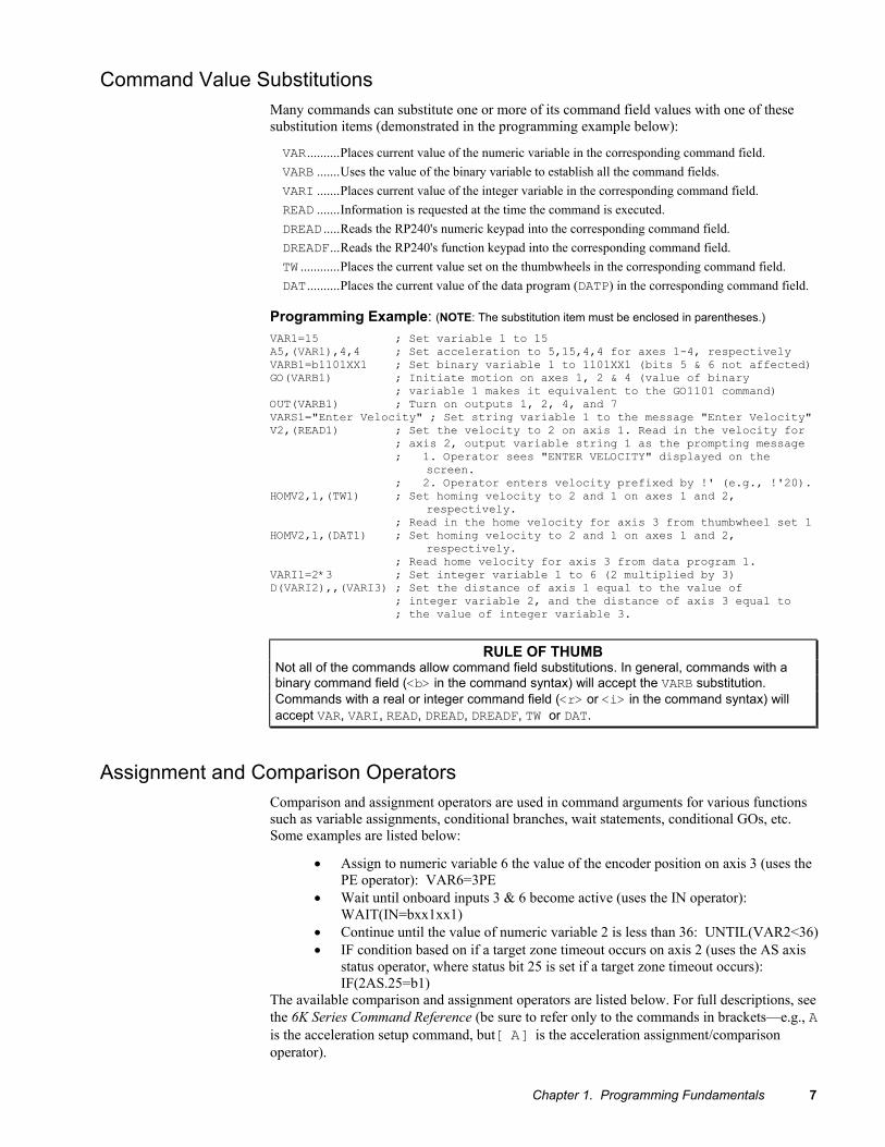
Command Value Substitutions Many commands can substitute one or more of its command field values with one of these substitution items (demonstrated in the programming example below):
VAR ..........Places current value of the numeric variable in the corresponding command field. VARB .......Uses the value of the binary variable to establish all the command fields. VARI .......Places current value of the integer variable in the corresponding command field. READ .......Information is requested at the time the command is executed. DREAD .....Reads the RP240's numeric keypad into the corresponding command field. DREADF...Reads the RP240's function keypad into the corresponding command field. TW ............Places the current value set on the thumbwheels in the corresponding command field. DAT ..........Places the current value of the data program (DATP) in the corresponding command field.
Programming Example: (NOTE: The substitution item must be enclosed in parentheses.)
VAR1=15 ; Set variable 1 to 15 A5,(VAR1),4,4 ; Set acceleration to 5,15,4,4 for axes 1-4, respectively VARB1=b1101XX1 ; Set binary variable 1 to 1101XX1 (bits 5 & 6 not affected) GO(VARB1) ; Initiate motion on axes 1, 2 & 4 (value of binary ; variable 1 makes it equivalent to the GO1101 command) OUT(VARB1) ; Turn on outputs 1, 2, 4, and 7 VARS1="Enter Velocity" ; Set string variable 1 to the message "Enter Velocity" V2,(READ1) ; Set the velocity to 2 on axis 1. Read in the velocity for ; axis 2, output variable string 1 as the prompting message ; 1. Operator sees "ENTER VELOCITY" displayed on the
screen. ; 2. Operator enters velocity prefixed by !' (e.g., !'20). HOMV2,1,(TW1) ; Set homing velocity to 2 and 1 on axes 1 and 2,
respectively. ; Read in the home velocity for axis 3 from thumbwheel set 1 HOMV2,1,(DAT1) ; Set homing velocity to 2 and 1 on axes 1 and 2,
respectively. ; Read home velocity for axis 3 from data program 1. VARI1=2*3 ; Set integer variable 1 to 6 (2 multiplied by 3) D(VARI2),,(VARI3) ; Set the distance of axis 1 equal to the value of ; integer variable 2, and the distance of axis 3 equal to ; the value of integer variable 3.
RULE OF THUMB Not all of the commands allow command field substitutions. In general, commands with a binary command field (<b> in the command syntax) will accept the VARB substitution. Commands with a real or integer command field (<r> or <i> in the command syntax) will accept VAR, VARI, READ, DREAD, DREADF, TW or DAT.
Assignment and Comparison Operators Comparison and assignment operators are used in command arguments for various functions such as variable assignments, conditional branches, wait statements, conditional GOs, etc. Some examples are listed below:
• Assign to numeric variable 6 the value of the encoder position on axis 3 (uses the PE operator): VAR6=3PE
• Wait until onboard inputs 3 & 6 become active (uses the IN operator): WAIT(IN=bxx1xx1)
• Continue until the value of numeric variable 2 is less than 36: UNTIL(VAR2<36) • IF condition based on if a target zone timeout occurs on axis 2 (uses the AS axis
status operator, where status bit 25 is set if a target zone timeout occurs): IF(2AS.25=b1)
The available comparison and assignment operators are listed below. For full descriptions, see the 6K Series Command Reference (be sure to refer only to the commands in brackets—e.g., A is the acceleration setup command, but [ A ] is the acceleration assignment/comparison operator).

8 6K Series Programmer’s Guide
* denotes operators that have a correlated status display command. (e.g., To see a full-text description of each axis status bit accessed with the AS operator, send the TASF command to the 6K controller.) See page 226.
A ...................Acceleration AD.................Deceleration ANI ..............Voltage at the analog inputs on an expansion I/O brick (see page 76 for bit patterns) * ANO ..............Voltage at the analog outputs on an expansion I/O brick (see page 76 for bit patterns) * AS.................Axis status * ASX ..............Extended axis status (additional axis status items) * D ...................Distance DAC ..............Digital-to-analog converter (output voltage) value * DAT ..............Data program number DKEY ............Value of RP240 Key DPTR ............Data pointer location * DREAD .........Data from the numeric keypad on the RP240 DREADF .......Data from the function keypad on the RP240 ER.................Error status * FB.................Position of current selected feedback sources * FS.................Following status * IN................. Input status (input bit patterns, see page 76) * INO .............. “Other” input status (ENABLE input reported with bit 6) * LIM ..............Limit status (end-of-travel limits and home limits) * MOV ..............Axis moving status NMCY ............Current master cycle number * OUT ..............Output status (output bit patterns, see page 76) * PANI ............Position of analog input, at 205 counts/volts unless otherwise scaled (servo axes) * PC.................Commanded position * PCC ..............Captured commanded position * PCE ..............Captured encoder position * PCME ............Captured master encoder position * PCMS ............Captured master cycle position * PER ..............Position error (servo axes only) * PME ..............Current master encoder position * PMAS ............Current master cycle position * PE.................Position of master encoder * PSHF ............Net position shift since constant Following ratio * PSLV ............Current commanded position of the slave axis * READ ............Read a numeric value to a numeric variable (VAR) SC.................Controller status * SCAN ............Runtime of the last scanned PLC program * SEG ..............Number of segments available in Compiled Profile memory * SS.................System status * SWAP ............Current active status of tasks * TASK ............Number of the controlling task * TIM ..............Timer value * TRIG ............Trigger interrupt status * TW.................Thumbwheel data read US.................User status * V ...................Velocity (programmed) VAR ..............Numeric variable substitution VARI ............ Integer variable substitution VARB ............Binary variable substitution VEL ..............Velocity (commanded by the controller) * VELA ............Velocity (actual, as measured by a position feedback device) * VMAS ............Current velocity of the master axis *
Bit Select Operator The bit select operator (.) makes it easier to base a command argument on the condition of one specific status bit. For example, if you wish to base an IF statement on the condition that a user fault input is activated (error status bit 7 is a binary status bit that is “1” if a user fault occurred and “Ø” if it has not occurred), you could use this command: IF(ER=bxxxxxx1). Using a bit select operator, you could instead use this command: IF(ER.7=b1).
NOTE: You can use a bit select operator to set a particular status bit (e.g., to turn on onboard programmable output 5, you would type the OUT.5-1 command; to enable error-checking bit 4 to check for drive faults, you would type the ERROR.4-1 command). You can also check specific status bits (e.g., to check axis 2’s axis status bit 25 to see if a target zone timeout

Chapter 1. Programming Fundamentals 9
occurred, type the 2TAS.25 command and observe the response).
Binary and Hex Values
When making assignments with or comparisons against binary or hexadecimal values, you must precede the binary value with the letter “b” or “B”, and the hex value with “h” or “H”. Examples: IF(IN=b1xØ1) and IF(IN=h7F). In the binary syntax, an “x” simply means the status of that bit is ignored. Refer also to Using Binary Variables (page 22).
Related Operator Symbols
Command arguments include special operator symbols (e.g., +, /, &, ', >=, etc.) to perform bitwise, mathematical, relational, logical, and other special functions. These operators are described in detail, along with programming examples, at the beginning of the Command Descriptions section of the 6K Series Command Reference.
Programmable Inputs and Outputs Bit Patterns I/O pin outs, specifications, and circuit drawings are provided in each 6K Series Hardware Installation Guide.
The 6K product has programmable inputs and outputs. The total number of onboard inputs and outputs (trigger inputs, limit inputs, digital outputs) depends on the product. The total number of expansion inputs and outputs (analog inputs, digital inputs and digital outputs) depends on your configuration of expansion I/O bricks connected to the “EXPANSION I/O” connector.
These programmable I/O are represented by binary bit patterns, and it is the bit pattern that you reference when programming and checking the status of specific inputs and outputs. The bit pattern is referenced in commands like WAIT(IN.4=b1), which means wait until onboard programmable input 4 (TRG-2B) becomes active. To ascertain your product’s I/O offering and bit patterns, see Chapter 3 (page 76).
Creating Programs
Debugging Programs: Refer to page 225 for methods to isolate and resolve programming problems.
A program is a series of commands. These commands are executed in the order in which they are programmed. Immediate commands (commands that begin with an exclamation point [!]) cannot be stored in a program. Only buffered commands can be used in a program. Refer to the program example below.
A subroutine is defined the same as a program, but it is executed with an unconditional branch command, such as GOSUB, GOTO, or JUMP, from another program (see page 23 for details about unconditional branching). Subroutines can be nested up to 16 levels deep. NOTE: The 6K family does not support recursive calling of subroutines.
Compiled profiles & PLC programs are defined like programs, using the DEF and END commands, but are compiled with the PCOMP command and executed with the PRUN command (PLC programs are usually launched in PLC Scan Mode with the SCANP command). Compiled profiles and PLC programs also affect a different part of the product's memory, called compiled memory. A compiled profile could be a multi-axis contour (a series of arcs and lines), an individual axis profile (a series of GOBUF commands), or a compound profile (combination of multi-axis contours and individual axis profiles). A compiled PLC program is a pre-compiled program that mimics PLC functionality by scanning through the I/O faster than in normal program execution. For information on contouring, see page 124; for information on compiled individual axis profiles, see page 136; and for information on PLC programs, see page 104.

10 6K Series Programmer’s Guide
Program Example The illustration below identifies the elements that comprise the general structure of a program.
; ********************************************************* ; This is a program that executes a trapezoidal motion ; profile on axes 1 and 2 ; ********************************************************* DEL motion ; (a precaution) Delete program called "motion"
DEF motion ; Begin definition of program called "motion"
DRIVE11 ; Enable drives on axes 1 and 2 MC00 ; Set position mode to preset on both axes A20,10 ; Set accel on axis 1 to 20 units/sec/sec, and ; Set accel on axis 2 to 10 units/sec/sec V8,5 ; Set velocity on axis 1 to 8 units/sec, and ; Set velocity on axis 2 to 5 units/sec D100000,75000 ; Set distance to 100,000 counts on axis 1, and ; Set distance to 75,000 counts on axis 2 GO11 ; Execute motion on axes 1 and 2
END ; End definition of program called "motion"
Use the Wizards in Motion Planner Motion Planner provides wizards that make it easy to create your program. Below is a partial list of the wizards available.
• Application Wizards (for program structure guidance) − Standard Application − Multitasking Application
• Program Wizards − Setup Program − Main Program − User Program − Error Program
• Setup Wizards − Drive − Feedback − Scaling − Limit − Servo Tuner − On-board I/O − Expansion I/O − Jogging − Joystick − Variable
• Action Wizards − Motion − Home − Output − If − Loop − Wait − Assignment − Target Zone − Registration
These are command line comments, comprising a semi-colon and text. The comments are separated from the command by a tab. A carriage return is placed at the end of each command line.
Use DEF to begin defining the program.
Contents of the program.
Use DEL to delete the program (a precaution).
Use END to finish defining the program.

Chapter 1. Programming Fundamentals 11
Storing Programs After a program or compiled program/profile is defined (DEF) or downloaded to the 6K controller, it is automatically stored in non-volatile memory (battery-backed RAM). Information on controlling memory allocation is provided below (Memory Allocation, see page 11).
Memory Allocation Your controller's memory has two partitions: one for storing programs and one for storing compiled profiles & PLC programs. The allocation of memory to these two areas is controlled with the MEMORY command.
“Programs” vs. ”Compiled Profiles & PLC Programs” Programs are defined with the DEF and END commands, as demonstrated in the Program
Example on page 10.
Compiled Profiles & PLC Programs are defined like programs, using the DEF and END commands, but are compiled with the PCOMP command and executed with the PRUN command (PLC programs are usually executed in PLC Scan Mode with the SCANP). A compiled profile could be a multi-axis contour (a series of arcs and lines), an individual axis profile (a series of GOBUF commands), or a compound profile (combination of multi-axis contours and individual axis profiles). A PLC program is a pre-compiled program that mimics PLC functionality by scanning through the I/O faster than in normal program execution.
Programs intended to be compiled are stored in program memory. After they are compiled with the PCOMP command, they remain in program memory and the segments (see diagram below) from the compiled program are stored in compiled memory. The TDIR report indicates which programs are compiled as compiled profiles (“COMPILED AS A PATH”) and which programs are compiled as PLC programs (“COMPILED AS A PLC PROGRAM”).
For information on contouring, see page 124; for information on compiled individual axis profiles, see page 136; and for information on PLC programs, see page 104.
MEMORY command
syntax (example)
������������������������������� ��������������������������������������������������������� ������� ��� ����� ������������������������� ��� ������� ����������!������ ���������� �������������� ��"
������������� �������������������������������������� ������ ��� ����� ��������!��##����������� ������������
����
�����
����
���
��
�� ����� �" ������������� "
������� ��
������
�����
����
����
����
����
����
����
����
����
�$��� ����������"
������ ��
���
�
���
���
���
���
��������������
� ������������������� ���������������������� ��������������������� ������������������������������
��������������������������� ���������������������������������������������

12 6K Series Programmer’s Guide
The table below identifies memory allocation defaults and limits for all 6K Series products. When specifying the memory allocation, use only even numbers. The minimum storage capacity for one partition area (program or compiled) is 1,000 bytes.
Feature All Other Products Total memory (bytes) 300,000 Default allocation (program,compiled) 150000,150000 Maximum allocation for programs 299000,1000 Maximum allocation for compiled profiles & PLC programs
1000,299000
Maximum No. of programs 400 Maximum No. of labels 600 Maximum No. of compiled profiles & PLC programs 300 Maximum No. of compiled profile segments 2069 Maximum No. of numeric variables (VAR) 225 Maximum No. of integer variables (VARI) 225 Maximum No. of binary variables (VARB) 125 Maximum No. of string variables (VARS) 25
When teaching variable data to a data program (DATP), be aware that the memory required for each data statement of four data points (43 bytes) is taken from the memory allocation for program storage (see Variable Arrays in Chapter 3, page 94, for details).
CAUTION Using a memory allocation command (e.g., MEMORY200000,100000) will erase all existing programs and compiled profile segments & PLC programs. However, issuing the MEMORY command without parameters (i.e., type MEMORY <cr> to request the status of how the memory is allocated) will not affect existing programs or compiled segments/programs.
Checking Memory Status To find out what programs reside in your controller's memory, and how much of the available memory is allocated for programs and compiled profile segments, issue the TDIR command (see example response below). Entering the TMEM command or the MEMORY command (without parameters) will also report the available memory for programs and compiled profile segments.
Sample response to TDIR command
*1 - SETUP USES 345 BYTES *2 - PIKPRT USES 333 BYTES *149322 OF 150000 BYTES (98%) PROGRAM MEMORY REMAINING *1973 OF 1973 SEGMENTS (100%) COMPILED MEMORY REMAINING
Two system status bits (reported with the TSS and SS commands) are available to check when compiled profile segment storage is 75% full or 100% full. System status bit 29 is set when segment storage reaches 75% of capacity; bit 30 indicates when segment storage is 100% full.

Chapter 1. Programming Fundamentals 13
Executing Programs (options) Following is a list of the primary options for executing programs stored in your controller:
Method Description See Also Execute from a terminal emulator
Type in the name of the program and press enter; or write a program to prompt the operator to select a program from the terminal.
-------
Execute as a subroutine from a “main” program
Use a branch (GOTO, GOSUB, or JUMP) from the main program to execute another stored program.
Page 23
Execute automatically when the controller is powered up
Assign a specific program as a startup program with the STARTP command. When you RESET or cycle power to the controller, the startup program is automatically executed.
Page 13
Execute from a PLC program
Write a PLC program that executes a program (using EXE or PEXE) based on a specific condition (e.g., input state). Use the SCANP command to launch the PLC program in the PLC Scan Mode.
Page 104
Execute a specific program with BCD weighted inputs
Define programmable inputs to function as BCD select inputs, each with a BCD weight. A specific program (identified by its number) is executed based on the combination of active BCD inputs. Related commands: INSELP and INFNCi-B or LIMFNCi-B.
Page 82
Execute a specific program with a dedicated input
Define a programmable input to execute a specific program (by number). Related commands: INSELP and INFNCi-iP or LIMFNCi-P.
Page 88
“Call” from a high-level program
Using a programming language such as BASIC or C, write a program that enables the computer to monitor processes and orchestrate motion and I/O by executing stored programs (or individual commands) in the controller.
Page 118
Execute from an RP240 (remote operator interface)
Execute a stored program from the RUN menu in the RP240’s standard menu system.
Page 111
Execute from your own custom Windows program
Use a programming language (e.g., Visual Basic, Visual C++, etc.) and the 6K Communications Server (provided on the Motion Planner CD) to create your own windows application to control the 6K product.
---------
Creating and Executing a Setup Program The intent of the Setup program is to place the 6K controller in a ready state for subsequent motion control. The setup program must be called from the “main” program for your application; or you can designate (with STARTP) the setup program as the program to be is automatically executed when the 6K product is powered up or when the RESET command is executed. The setup program typically contains elements such as feedback device configuration, tuning gain selections, programmable I/O definitions, scaling, homing configuration, variable initialization, etc. (more detail on these “basic” features is provided in Chapter 3, Basic Operation Setup).
The basic process of creating a setup program is:
1. Create a program to be used as the setup program. 2. Save the program and download it to the 6K product. 3. Execute the STARTP command to assign your new program as the “start-up” program
(e.g., STARTP setup assigns the program called “setup” as the start-up program). The next time the controller is powered up or reset, the assigned STARTP program will be executed. Or call the setup program from the main program for your application.

14 6K Series Programmer’s Guide
Use Motion Planner’s Setup wizard to help you create the basic configuration program. By simply responding to a series of dialog boxes, a program is created with a specific name (as if you created it in the usual process with the DEF and END commands). You can further edit this program in Motion Planner's Editor if you wish. Use the following procedure:
1. From the main Editor window, click the “Standard Application” wizard button (located on the right-hand side of the screen under Application Wizards) and select “Setup” and “Main” from the dialog. When you click “Finish”, Motion Planner places a Setup program icon and a Main program icon in the Editor window.
2. Double-click the Setup program icon to launch the wizard. Complete the wizard dialogs and click “Finish” to complete the wizard. (The next time you open the icon, you will see a program editor with the code resulting from the setup wizard.) Setup elements include:
• Product selection • Drives • Feedback (encoder, analog input) • Scaling • Hardware end-of-travel limits • Servo tuning
3. Double-click the Main program icon to launch the wizard. Select this program as the program to launch when the 6K controller is reset or powered up (this is equivalent to the STARTP command function). In the dialog for selecting the Setup Program, select the program developed in step 2 above.
4. Save the Editor files.
5. Download the files to the 6K controller.
Program Security Issuing the INFNCi-Q or LIMFNCi-Q command enables the Program Security feature and assigns the Program Access function to the specified programmable input. The “i” represents the number of the programmable input to which you wish to assign the function (see page 76 programmable input bit patterns for your product).
The program security feature denies you access to the DEF, DEL, ERASE, MEMORY, INFNC, and LIMFNC commands until you activate the program access input. Being denied access to these commands effectively restricts altering the user memory allocation. If you try to use these commands when program security is active (program access input is not activated), you will receive the error message *ACCESS DENIED.
For example, once you issue the INFNC5-Q command, onboard input 5 is assigned the program access function and access to the DEF, DEL, ERASE, MEMORY, INFNC, and LIMFNC commands will be denied until you activate onboard input 5.
NOTE: To regain access to these commands without the use of the program access input, you must issue the INEN command to disable the program security input, make the required user memory changes, and then issue the INEN command to re-enable the input. For example, if input 3 on I/O brick 2 is assigned as the Program Security input, use 2INEN.3=1 to disable the input and leave it activated, make the necessary user memory changes, and then use 2INEN.3=E to re-enable the input.

Chapter 1. Programming Fundamentals 15
Controlling Execution of Programs and the Command Buffer The 6K controller command buffer is capable of storing 2000 characters waiting to be processed. (This is separate from the memory allocated for program storage – see Memory Allocation, page 11.) COMEXC affects command execution. Three additional commands, COMEXL, COMEXR and COMEXS, affect the execution of programs and the command buffer.
COMEXC (Continuous Command Execution) The COMEXC1 command enables the Continuous Command Execution Mode (default is COMEXC0). This mode allows the program to continue to the next command before motion is complete. This is useful for:
• Monitoring other processes while motion is occurring • Performing calculations in advance of motion completion • Pre-emptive GOs — executing a new profile with new attributes (distance,
accel/decel, velocity, positioning mode, and Following ratio ) before motion is complete: The motion profile underway is pre-empted with a new profile when a new GO is issued. The new GO both constructs and launches the pre-empting profile. Pre-emptive GOs are appropriate when the desired motion parameters are not known until motion is already underway. For a detailed description, see On-The-Fly Motion on page 151.
• Pre-process the next move while the current move is in progress (see CAUTION). This reduces the processing time for the subsequent move to only a few microseconds.
CAUTION: Avoid executing moves prematurely
With continuous command execution enabled (COMEXC1), if you wish motion to stop before executing the subsequent move, place a WAIT(AS.1=bØ) statement before the subsequent GO command. If you wish to ensure the load settles adequately before the next move, use the WAIT(AS.24=b1) command instead (this requires you to define end-of-move settling criteria — see Target Zone Mode on page 74 for details).
In the programming example below, by enabling the continuous command execution mode (COMEXC1), the controller is able to turn on output 3 after the encoder moves 4000 units of its 125000-unit move. Normally, with COMEXC disabled (COMEXCØ), command processing would be temporarily stopped at the GO1 command until motion is complete.
Programming Example (portion of program only) COMEXC1 ;Enable continuous command execution mode D125000 ;Set distance V2 ;Set velocity A10 ;Set acceleration GO1 ;Initiate motion on axis 1 WAIT(1PE>4000) ;Wait for the encoder position to exceed 4000 OUTXX1 ;Turn on onboard programmable output 3 WAIT(AS.1=b0) ;Wait for motion to complete on axis 1 (AS bit 1 = zero) OUTXX0 ;Turn off onboard programmable output 3
COMEXL (Save Command Buffer on Limit)
For more information on end-of-travel limits,
see page 57.
The COMEXL command enables saving the command buffer and maintaining program execution when a hardware or software end-of-travel limit is encountered. COMEXL is axis specific (e.g., COMEXL1xx1xxx1 enables saving the buffer for axes 1, 4, and 8).
• COMEXL0: (This is the default setting.) When a limit is hit, every command in the command buffer will be discarded and program execution will be terminated.
• COMEXL1: When a limit is hit, all remaining commands in the command buffer will remain in the command buffer (excluding the command being executed at the time the limit is hit).

16 6K Series Programmer’s Guide
COMEXR (Effect of Pause/Continue Input) The COMEXR command affects whether a “Pause” input (i.e., an input configured as a pause/continue input with the INFNCi-E command or the LIMFNCi-E command) will pause only program execution or both program execution and motion.
COMEXRØ: (This is the default setting.) Upon receiving a pause input, only program execution will be paused; any motion in progress will continue to its predetermined destination. Releasing the pause input or issuing a !C command will resume program execution.
COMEXR1: Upon receiving a pause input, both motion and program execution will be paused; the motion stop function is used to halt motion. After motion has come to a stop (not during deceleration), you can release the pause input or issue a !C command to resume motion and program execution.
Other Ways to Pause • Issue the PS command before entering a series of buffered commands (to cause motion,
activate outputs, etc.), then issue the !C command to execute the commands. • While program execution is in progress, issuing the !PS command stops program execution,
but any move currently in progress will be completed. Resume program execution with the !C command.
COMEXS (Save Command Buffer on Stop) The COMEXS command determines the impact on motion, program execution, and the command buffer when the 6K receives a Stop command (S, !S, S1, or !S1) or an external Stop input (an input assigned a stop function with INFNCi-D or LIMFNCi-D).
COMEXS0: Under factory default conditions (COMEXS0), when the 6K receives a stop command (S, !S, S1, or !S1) or a stop input (INFNCi-D or LIMFNCi-D), the following will happen: • Motion decelerates to a stop, using the present AD and ADA deceleration values.
The motion profile cannot be resumed. • If S, !S or Stop input:
– All commands in the 6K’s command buffer are discarded. – Program execution is terminated and cannot be resumed.
• If S1, or !S1 (an axis number is included in the command): – All commands in the 6K’s command buffer are retained. – Program execution continues.
COMEXS1: Using the COMEXS1 mode, the 6K allows more flexibility in responding to stop conditions, depending on the stop method (see table below).
Stop Method
What Stops? Motion Program
Resume Motion Profile. (Allow resume with a !C command or a resume input * )
Resume Program. (Allow resume with a !C command or a resume input * )
Save Command Buffer. (Save the commands that were in the command buffer when the stop was commanded)
!S or S Yes Yes Yes Yes Yes !S1 or S1 Yes No No No Yes Stop input Yes Yes No Yes Yes Pause input *
(if COMEXR1) Yes Yes Yes Yes Yes
Pause input * (if COMEXR0)
No Yes No Yes Yes
* A Pause input is an input configured with the INFNCi-E command or the LIMFNCi-E command. This is also the Resume input that can be used to resume motion and program execution after motion is stopped.
COMEXS2: Using the COMEXS2 mode, the 6K responds as it does in the COMEXS0 mode, with the exception that you can still use the program-select inputs to select programs (INSELP value is retained). The program-select input functions are: BCD select (INFNCi-B or LIMFNCi-B), and one-to-one select (INFNCi-P or LIMFNCi-P).

Chapter 1. Programming Fundamentals 17
Restricted Commands During Motion When motion is in progress on a given axis (or task), some commands cannot have their parameters changed until motion is complete (see table below).
For the commands identified in the table, if the continuous command execution mode is enabled (COMEXC1) and you try to enter new command parameters, you will receive the error response MOTION IN PROGRESS. If the continuous command execution mode in disabled (COMEXCØ), which is the default setting, you will receive the response MOTION IN PROGRESS only if you precede the command with the immediate (!) modifier (e.g., !V2Ø); if you enter a command without the immediate modifier (e.g., V2Ø), you will not receive an error response and the new parameter will be ignored and the old parameter will remain in effect.
Multi-Tasking If you are using multi-tasking, the restriction on commands is applicable only for the task to which the command is direct. For example, suppose axes 1 and 2 are associated with Task 1 (TSKAX1,2) and axes 3 and 4 are associate with Task 2 (TSKAX3,4). If motion is in progress on axes 1 and 2, Task 1 is considered “in motion” and Task 1 cannot execute a command from the list below. However, while motion is in progress in Task 1 and not Task 2, Task 2 can execute these commands without encountering an error.
All of the commands in the table below, except for SCALE, are axis-dependent. That is, if one axis is moving you can change the parameters on the other axes, provided they are not in motion.
Command Description Command Description CMDDIR.........Commanded Direction Polarity JOY............... Joystick Mode Enable DRES .............Drive Resolution JOYA............. Joystick Acceleration DRIVE ...........Drive Shutdown JOYAA .......... Average Joystick Acceleration ENCPOL.........Encoder Polarity JOYAD .......... Joystick Deceleration ERES .............Encoder Resolution JOYADA ........ Average Joystick Deceleration FOLEN ...........Following Mode Enable JOYVH .......... Joystick Velocity High GOL ............... Initiate Linear Interpolated Motion JOYVL .......... Joystick Velocity Low HOM ...............Go Home LHAD............. Hard Limit Deceleration HOMA .............Home Acceleration LHADA .......... Average Hard Limit Deceleration HOMAA ...........Average Home Acceleration LSAD............. Soft Limit Deceleration HOMAD ...........Home Deceleration LSADA .......... Average Soft Limit Deceleration HOMADA.........Average Home Deceleration PSET............. Establish Absolute Position HOMV .............Home Velocity SCALE .......... Enable/Disable Scale Factors * HOMVF ...........Home Final Velocity SCLA............. Acceleration Scale Factor JOG ...............Jog Mode Enable SCLD............. Distance Scale Factor JOGA .............Jog Acceleration SCLV............. Velocity Scale Factor JOGAA ...........Average Jog Acceleration JOGAD ...........Jog Deceleration JOGADA.........Average Jog Deceleration JOGVH ...........Jog Velocity High JOGVL ...........Jog Velocity Low
* If any axis is in motion, you will cause an error if you attempt to change this command's parameters.

18 6K Series Programmer’s Guide
Variables 6K Series controllers have four types of variables, each designated with a different command. All four types are automatically stored in non-volatile memory.
Type Command Quantity Function Numeric (real)
VAR 225 Store real numeric data (range is ±999,999,999.99999999). Can be used to perform mathematical (=, +, -, *, /, SQRT), trigonometric (ATAN, COS, PI, SIN, TAN), and Boolean (&, |, ^, ~) operations. Can also be used to store (“teach”) variable data in variable arrays (called data programs) and later use the stored data as a source for motion program parameters (see Variable Arrays on page 94 for details).
Integer VARI 225 Store integer numeric data (range is ±2,147,483,647). Can be used to perform mathematical (=, +, -, *, /) and Boolean (&, |, ^, ~) operations.
Binary VARB 125 Store 32-bit binary or hexadecimal values. Can also store the binary status bits from status registers. Frequently used registers are: inputs (IN), outputs (OUT), limits (LIM), system (SS), Following (FS), axis (AS & ASX), and error (ER). For example, the VARB2=IN.3 command assigns the binary state of input 12 to binary variable 2. Also use to perform bitwise operations (&, |, ^, ~, >>, <<).
String VARS 25 Store message strings of 50 characters or less. These message strings can be predefined error messages, user messages, etc. The programming example in the Command Value Substitutions (page 7) demonstrates the use of a string variable.
Enhancements as of OS revision 5.1.0: • Copy one VARS variable to another VARS variable. VARSn=VARSm can be used, as well as variable substitutions for “n” and “m”.
• VARS message string was increased from 20 to 50 characters.
NOTE: Variables do not share the same memory (e.g., VAR1, VARI1, VARB1, and VARS1 can all exist at the same time and operate separately).
Converting Between Binary and Numeric Variables Using the Variable Type Conversion (VCVT) operator, you can convert numeric (VAR or VARI) values to binary (VARB) values, and vice versa. The operation is a signed operation as the binary value is interpreted as a two's complement number. Any don't cares (x) in a binary value is interpreted as a zero (Ø).
If the mathematical statement's result is a numeric value, then VCVT converts binary values to numeric values. If the statement's result is a binary value, then VCVT converts numeric values to binary values.
Numeric to Binary Example Descr ip t ion/Response VAR1=-5 Set numeric variable value = -5 VARB1=VCVT(VAR1) Convert the numeric value to a binary value VARB1 *VARB1=1101_1111_1111_1111_1111_1111_1111_1111
Binary to Numeric Example Descr ip t ion/Response VARB1=b0010_0110_0000_0000_0000_0000_0000_0000 Set binary variable = +100.0 VAR1=VCVT(VARB1) Convert binary value to numeric VAR1 *VAR1=+100.0

Chapter 1. Programming Fundamentals 19
Using Numeric (VAR and VARI) Variables
NOTES • The examples below show the use of real numeric variables (VAR). Integer variables can
be used in the same operations with these exceptions: - Values are truncated to nearest integer value - Operations using square root (SQRT) and trigonometric (ATAN, COS, PI, SIN, TAN) operators are not allowed
• Some numeric variable operations reduce precision. The following operations reduce the precision of the return value: Division and Trigonometric functions yield 5 decimal places; Square Root yields 3 decimal places; and Inverse Trigonometric functions yield 2 decimal places.
Mathematical Operations
The following examples demonstrate how to perform math operations with numeric variables. Operator precedence occurs from left to right (e.g., VAR1=1+1+1∗3 sets VAR1 to 9, not 5).
Addition (+)
Example Response VAR1=5+5+5+5+5+5+5 VAR1 *VAR1=35.0 VAR23=1000.565 VAR11=VAR1+VAR23 VAR11 *VAR11=+1035.565 VAR1=VAR1+5 VAR1 *VAR1=+40.0
Subtraction (-) Example Response VAR3=20-10 VAR20=15.5 VAR3=VAR3-VAR20 VAR3 *VAR3=-5.5
Multiplication (*) Example Response VAR3=10 VAR3=VAR3*20 VAR3 *VAR3=+200.0
Division (/) Example Response VAR3=10 VAR20=15.5 VAR20 *+15.5 VAR3=VAR3/VAR20 VAR3 *+0.64516 VAR30=75 VAR30 *+75.0 VAR19=VAR30/VAR3 VAR19 *+116.25023
Square Root (SQRT) Example Response VAR3=75 VAR20=25 VAR3=SQRT(VAR3) VAR3 *+8.660 VAR20=SQRT(VAR20)+SQRT(9) VAR20 *+8.0
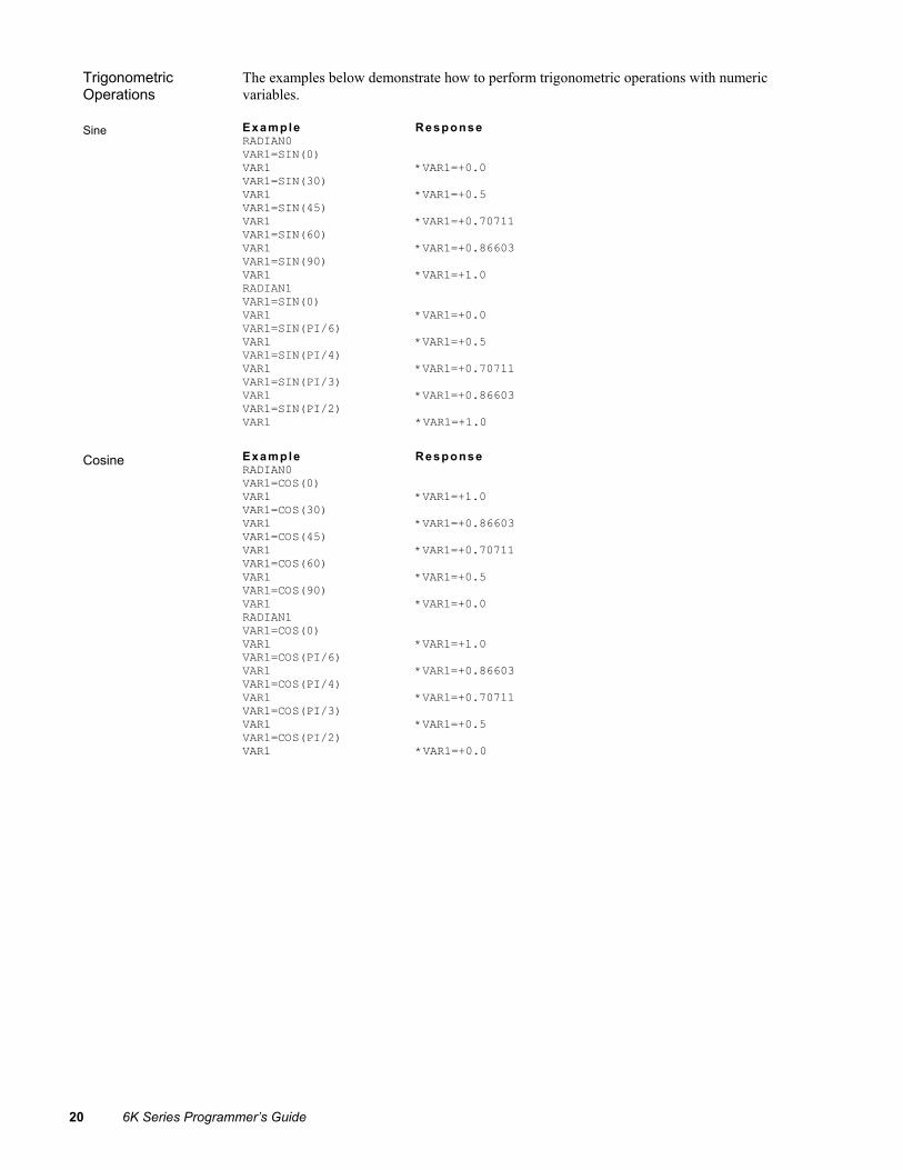
20 6K Series Programmer’s Guide
Trigonometric Operations
The examples below demonstrate how to perform trigonometric operations with numeric variables.
Sine Example Response RADIAN0 VAR1=SIN(0) VAR1 *VAR1=+0.0 VAR1=SIN(30) VAR1 *VAR1=+0.5 VAR1=SIN(45) VAR1 *VAR1=+0.70711 VAR1=SIN(60) VAR1 *VAR1=+0.86603 VAR1=SIN(90) VAR1 *VAR1=+1.0 RADIAN1 VAR1=SIN(0) VAR1 *VAR1=+0.0 VAR1=SIN(PI/6) VAR1 *VAR1=+0.5 VAR1=SIN(PI/4) VAR1 *VAR1=+0.70711 VAR1=SIN(PI/3) VAR1 *VAR1=+0.86603 VAR1=SIN(PI/2) VAR1 *VAR1=+1.0
Cosine Example Response RADIAN0 VAR1=COS(0) VAR1 *VAR1=+1.0 VAR1=COS(30) VAR1 *VAR1=+0.86603 VAR1=COS(45) VAR1 *VAR1=+0.70711 VAR1=COS(60) VAR1 *VAR1=+0.5 VAR1=COS(90) VAR1 *VAR1=+0.0 RADIAN1 VAR1=COS(0) VAR1 *VAR1=+1.0 VAR1=COS(PI/6) VAR1 *VAR1=+0.86603 VAR1=COS(PI/4) VAR1 *VAR1=+0.70711 VAR1=COS(PI/3) VAR1 *VAR1=+0.5 VAR1=COS(PI/2) VAR1 *VAR1=+0.0

Chapter 1. Programming Fundamentals 21
Tangent Example Response RADIAN0 VAR1=TAN(0) VAR1 *VAR1=+0.0 VAR1=TAN(30) VAR1 *VAR1=+0.57735 VAR1=TAN(45) VAR1 *VAR1=+1.0 VAR1=TAN(60) VAR1 *VAR1=+1.73205 RADIAN1 VAR1=TAN(0) VAR1 *VAR1=+0.0 VAR1=TAN(PI/6) VAR1 *VAR1=+0.57735 VAR1=TAN(PI/4) VAR1 *VAR1=+1.0 VAR1=TAN(PI/3) VAR1 *VAR1=+1.73205
Inverse Tangent (Arc Tangent)
Example Response RADIAN0 VAR1=SQRT(2) VAR1=ATAN(VAR1/2) VAR1 *VAR1=+35.26 VAR1=ATAN(.57735) VAR1 *VAR1=+30.0
Boolean Operations 6K Series products have the ability to perform Boolean operations with numeric variables. The following examples illustrate this capability. Refer to the 6K Series Command Reference for more information on each operator (&, |, ^, and ~).
Boolean And (&) Example Response VAR1=5 VAR2=-1 VAR3=VAR1 & VAR2 VAR3 *VAR3=+0.0
Boolean Or (|) Example Response VAR1=5 VAR2=-1 VAR3=VAR1 | VAR2 VAR3 *VAR3=+1.0
Boolean Exclusive Or (^)
Example Response VAR1=5 VAR2=-1 VAR3=VAR1 ^ VAR2 VAR3 *VAR3=+1.0
Boolean Not (~) Example Response VAR1=5 VAR3=~(VAR1) VAR3 *VAR3=+0.0 VAR1=-1 VAR3=~(VAR1) VAR3 *VAR3=+1.0

22 6K Series Programmer’s Guide
Using Binary Variables The following examples illustrate the 6K Series product's ability to perform bitwise functions with binary variables.
Storing binary values. The 6K Series Language allows you to store binary numbers in the binary variables (VARB) command. The binary variables start at the left with the least significant bit, and increase to the right. For example, to set bit 1, 5, and 7 you would issue the command VARB1=b1xxx1x1. Notice that the letter b is required. When assigning a binary variable, any bit set to “x” remains “x” until set to “1” or “0”. Any bit that is unspecified is set to “x”. To change, or check, one bit without affecting the others, use the bit-select operator (e.g., use VARB1.3-1 to set only bit 3 of VARB1).
Example Response VARB1=b1101XX1 *VARB1=1101_XX1X_XXXX_XXXX_XXXX_XXXX_XXXX_XXXX
Storing hexadecimal values. Hexadecimal values can also be stored in binary variables (VARB). The hexadecimal value must be specified the same as the binary value—left is least significant byte, right is most significant. For example, to set bit 1, 5, and 7 you would issue the command VARB1=h15. Notice that the letter h is required. NOTE: When assigning a hexadecimal value to a binary variable, all unspecified bits are set to zero.
Example Response VARB1=h7FAD VARB1 *VARB1=1110_1111_0101_1011_0000_0000_0000_0000
Bitwise And (&) Example Response VARB1=b1101 VARB1 *VARB1=1101_XXXX_XXXX_XXXX_XXXX_XXXX_XXXX_XXXX VARB1=VARB1 & bXXX1 1101 VARB1 *VARB1=XX01_XX0X_XXXX_XXXX_XXXX_XXXX_XXXX_XXXX VARB1=h0032 FDA1 & h1234 43E9 VARB1 *VARB1=0000_0000_1100_0000_0010_1000_0101_1000
Bitwise Or (|) Example Response VARB1=h32FD VARB1 *VARB1=1100_0100_1111_1011_0000_0000_0000_0000 VARB1=VARB1 | bXXX1 1101 VARB1 *VARB1=11X1_1101_1111_1X11_XXXX_XXXX_XXXX_XXXX VARB1=h0032 FDA1 | h1234 43E9 VARB1 *VARB1=1000_0100_1100_0110_1111_1111_0111_1001
Bitwise Exclusive Or (^)
Example Response VARB1=h32FD ^ bXXX1 1101 VARB1 *VARB1=XXX1_1001_XXXX_XXXX_XXXX_XXXX_XXXX_XXXX VARB1=h0032 FDA1 ^ h1234 43E9 VARB1 *VARB1=1000_0100_0000_0110_1101_0111_0010_0001
Bitwise Not (~) Example Response VARB1=~(h32FD) VARB1 *VARB1=0011_1011_0000_0100_1111_1111_1111_1111 VARB1=~(b1010 XX11 0101) VARB1 *VARB1=0101_XX00_1010_XXXX_XXXX_XXXX_XXXX_XXXX
Shift Left to Right (>>)
Example Response VARB1=h32FD >> h4 VARB1 *VARB1=0000_1100_0100_1111_1011_0000_0000_0000 VARB1=b1010 XX11 0101 >> b11 VARB1 *VARB1=0001_010X_X110_101X_XXXX_XXXX_XXXX_XXXX
Shift Right to Left (<<)
Example Response VARB1=h32FD << h4 VARB1 *VARB1=0100_1111_1011_0000_0000_0000_0000_0000 VARB1=b1010 XX11 0101 << b11 VARB1 *VARB1=0XX1_1010_1XXX_XXXX_XXXX_XXXX_XXXX_X000
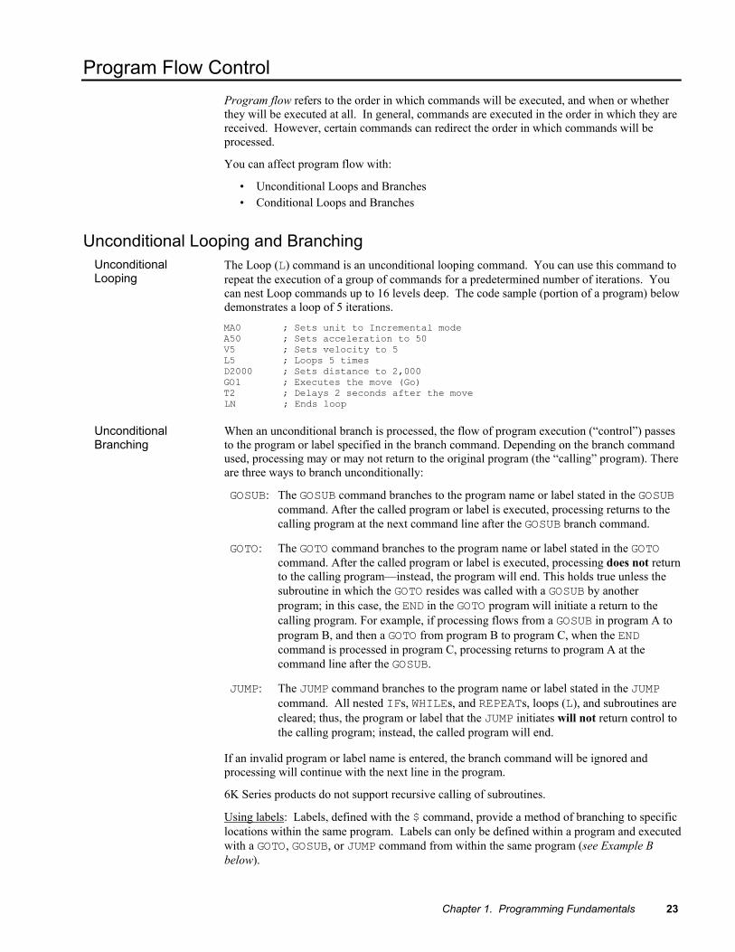
Chapter 1. Programming Fundamentals 23
Program Flow Control Program flow refers to the order in which commands will be executed, and when or whether they will be executed at all. In general, commands are executed in the order in which they are received. However, certain commands can redirect the order in which commands will be processed.
You can affect program flow with:
• Unconditional Loops and Branches • Conditional Loops and Branches
Unconditional Looping and Branching Unconditional Looping
The Loop (L) command is an unconditional looping command. You can use this command to repeat the execution of a group of commands for a predetermined number of iterations. You can nest Loop commands up to 16 levels deep. The code sample (portion of a program) below demonstrates a loop of 5 iterations. MA0 ; Sets unit to Incremental mode A50 ; Sets acceleration to 50 V5 ; Sets velocity to 5 L5 ; Loops 5 times D2000 ; Sets distance to 2,000 GO1 ; Executes the move (Go) T2 ; Delays 2 seconds after the move LN ; Ends loop
Unconditional Branching
When an unconditional branch is processed, the flow of program execution (“control”) passes to the program or label specified in the branch command. Depending on the branch command used, processing may or may not return to the original program (the “calling” program). There are three ways to branch unconditionally:
GOSUB: The GOSUB command branches to the program name or label stated in the GOSUB command. After the called program or label is executed, processing returns to the calling program at the next command line after the GOSUB branch command.
GOTO: The GOTO command branches to the program name or label stated in the GOTO command. After the called program or label is executed, processing does not return to the calling program—instead, the program will end. This holds true unless the subroutine in which the GOTO resides was called with a GOSUB by another program; in this case, the END in the GOTO program will initiate a return to the calling program. For example, if processing flows from a GOSUB in program A to program B, and then a GOTO from program B to program C, when the END command is processed in program C, processing returns to program A at the command line after the GOSUB.
JUMP: The JUMP command branches to the program name or label stated in the JUMP command. All nested IFs, WHILEs, and REPEATs, loops (L), and subroutines are cleared; thus, the program or label that the JUMP initiates will not return control to the calling program; instead, the called program will end.
If an invalid program or label name is entered, the branch command will be ignored and processing will continue with the next line in the program.
6K Series products do not support recursive calling of subroutines.
Using labels: Labels, defined with the $ command, provide a method of branching to specific locations within the same program. Labels can only be defined within a program and executed with a GOTO, GOSUB, or JUMP command from within the same program (see Example B below).

24 6K Series Programmer’s Guide
NOTE Be careful about performing a GOTO within a loop or branch statement area (i.e., between L & LN, between IF & NIF, between REPEAT & UNTIL, or between WHILE & NWHILE). Branching to a different location within the same program will cause the next L, IF, REPEAT, or WHILE statement encountered to be nested within the previous L, IF, REPEAT, or WHILE statement area, unless an LN, NIF, UNTIL, or NWHILE command has already been encountered.
** To avoid this nesting situation, use the JUMP command instead of the GOTO command.
Example A DESCRIPTION: The program cut1 is executed until it gets to the command GOSUB prompt. From there it branches unconditionally to the subroutine (actually a program) called prompt. The subroutine prompt queries the operator for the number of parts to process. After the part number is entered (e.g., operator enters the !'12 command to process 12 parts), the rest of the prompt subroutine is executed and control goes back to the cut1 program and resumes program execution with the next command after the GOSUB, which is MAØØ.
DEL cut1 ; Delete a program before defining it DEF cut1 ; Begin definition of program cut1 HOM11 ; Send axes 1 and 2 to the home position WAIT(1AS=b0XXX1 AND 2AS=b0XXX1) ; Wait for axes 1 and 2 to come ; to a halt at home GOSUB prompt ; Go to subroutine program called prompt MA00 ; Place axes 1 and 2 in the incremental mode A10,30 ; Set acceleration: axis 1 = 10, axis 2 = 30 AD5,12 ; Set deceleration: axis 1 = 5, axis 2 = 12 V5,8 ; Set velocity: axis 1 = 5, axis 2 = 8 D16000,100000 ; Set distance: axis 1 = 16,000; axis 2 = 100,000 OUT.3-1 ; Turn on onboard output number 3 T5 ; Wait for 5 seconds L(VAR2) ; Begin loop (number of loops = value of VAR2) GO11 ; Initiate moves on axes 1 and 2 T3 ; Wait for 3 seconds LN ; End loop OUT.3-0 ; Turn off onboard output number 3 END ; End definition of program cut1 DEF prompt ; Begin definition of program prompt VARS1="Enter part count >" ; Place message in string variable 1 VAR2=READ1 ; Prompt operator with string variable 1,
; and read data into numeric variable 2 ; NOTE: Type !' before the part count number.
END ; End definition of program prompt
Example B DESCRIPTION: This example demonstrates the use of labels ($).
DEL pick ; Delete a program before defining it DEF pick ; Begin definition of program pick GO1100 ; Initiate motion and axes 1 and 2 IF(VAR1=5) ; If variable 1 = 5, then execute commands ; between IF and ELSE. Otherwise, execute
; commands between ELSE and NIF GOTO pick1 ; Goto label pick1 ELSE ; Else part of IF statement GOTO pick2 ; Goto label pick2 NIF ; End of IF statement $ pick1 ; Define label for pick1 GO0011 ; Initiate motion on axes 3 and 4 BREAK ; Break out of current subroutine or program $ pick2 ; Define label for pick2 GO1001 ; Initiate motion on axes 1 and 4 END ; End definition of program pick

Chapter 1. Programming Fundamentals 25
Conditional Looping and Branching Conditional looping (REPEAT/UNTIL and WHILE/NWHILE) entails repeating a set of commands until or while a certain condition exists. In conditional branching (IF/ELSE/NIF), a specific set of commands is executed based on a certain condition. Both rely on the fulfillment of a conditional expression, a condition specified in the UNTIL, WHILE, or IF commands.
A wait command pauses command execution until a specific condition exists.
Flow Control Expression Examples
This section provides examples of expressions that can be used in conditional branching and looping commands (UNTIL, WHILE, and IF) and the wait command. These expressions can be constructed, in conjunction with relational and logical operators, with the following operands:
• Numeric variables and binary variables • Timer value • Inputs and outputs • Data read from the serial port • Current motion parameters and status • Data read from the RP240 • Current commanded and actual position • Following conditions • Error, axis, and system status • Multi-tasking conditions
Numeric and Binary Variables
A numeric variable (VAR or VARI) can be used within an expression if it is compared against another numeric variable, a value, or one of the comparison commands (see list on page 7). When comparing a variable against another value, variable, or comparison command, the relational operators (=, >, >=, <, <=, <>) and logical operators (AND, OR, NOT) are used.
Expression Descr ip t ion (VAR1<VAR2) True expression if variable 1 is less than variable 2 (VAR1>=2500) True expression if variable 1 is greater than or equal to 2500 (VAR1=1AD) True expression if variable 1 is equal to the decel of axis 1 (VAR1<VAR2 AND VAR4>1PE) True expression if variable 1 is less than variable 2 and variable 4 is
greater than the value of encoder 1
A binary variable (VARB) can be used within an expression, if the variable is compared against another binary variable, or a value. When comparing a variable against another value or variable, the relational operators (=, >, >=, <, <=, <>) and logical operators (AND, OR, NOT) are used.
Expression Descr ip t ion (VARB1<>VARB2) True expression if binary variable 1 is not equal to binary variable
2 (VARB1=b1101 X111) True expression if binary variable 1 is equal to 1101 X111 (VARB1<VARB2 AND VARB4>hF) True expression if binary variable 1 is less than binary variable 2
and binary variable 4 is greater than the hexadecimal value of F
Inputs and Outputs An input or output operand (ANI, ANO,IN, INO, LIM, OUT, TRIG) can be used within an expression, if the operand is compared against a binary variable or a binary or hexadecimal value. When making the comparison, the relational operators (=, >, >=, <, <=, <>) and logical operators (AND, OR, NOT) are used.
Expression Descr ip t ion (IN.3=b1) True expression if onboard input 3 is equal to 1 (LIM>h3) True expression if limit status is greater than hexadecimal 3
Current Motion Parameters and Status
Motion parameters consist of A, AD, D, V, VEL, status MOV. The motion parameters can be used within an expression, if the operand is compared against a numeric variable or value. The motion status operand must be compared against a binary variable or a binary or hexadecimal value. When making the comparison, the relational operators (=, >, >=, <, <=, <>) and logical operators (AND, OR, NOT) are used. (Following conditions are addressed below.)

26 6K Series Programmer’s Guide
Expression Descr ip t ion (VAR1<1VEL) True expression if the value of variable 1 is less than the commanded velocity of
axis 1 (1AD=25000) True expression if axis 1 deceleration equals 25000 (MOV=b00) True expression if moving status equals ØØ (axes 1 & 2 are not moving)
Current Commanded & Actual Position
The current commanded and actual positions (ANI, DAC, FB, PANI, PC, PCC, PCE, PCME, PCMS, PE, PER, PE, PMAS, PME, PSHF, PSLV) can be used within an expression, if the operand is compared against a numeric variable or value. When making the comparison, the relational operators (=, >, >=, <, <=, <>) and logical operators (AND, OR, NOT) are used.
Expression Descr ip t ion (VAR1<1FB) True expression if the value of variable 1 is less than the actual position (position of
the assigned feedback device) of axis 1 (2PC=4000) True expression if axis 2 commanded position equals 4000 (VAR1<1PME) True expression if VAR1 is < master encoder position of axis 1 (2PE=25000) True expression if axis 2 encoder position equals 25000
Error, Axis, and System Status
The error status, axis status, and system status operands (ER, AS, ASX, SS) can be used within an expression, if the operand is compared against a binary variable or a binary or hexadecimal value. When making the comparison, the relational operators (=, >, >=, <, <=, <>) and logical operators (AND, OR, NOT) are used. Refer to page 226 for a list of status bit functions.
Expression Descr ip t ion (ER.12=b1) True expression if error status bit 12 is equal to 1 (AS=h3FFD) True expression if axis status is equal to hexadecimal 3FFD
Timer Value The current timer value (TIM) can be used within an expression, if the operand is compared against a numeric variable or value. When making the comparison, the relational operators (=, >, >=, <, <=, <>) and logical operators (AND, OR, NOT) are used.
Expression Descr ip t ion (VAR1<TIM) True expression if the value of variable 1 is less than the timer value
Data Read from the Communications Port
The READ command can be used to input data from a serial port or the Ethernet port into a numeric variable. After the data has been read into a numeric variable, that variable can be used in an expression.
Example Descr ip t ion VARS8="ENTER DATA" Define message (string variable 8) VAR2=READ8 Send message (string variable 8) and then wait for immediate data to be
read (into numeric variable 2) !'88.3 Immediate data input (must type !' before the numeric value) IF (VAR2<=100) Evaluate expression to see if data read is < or equal to 100 . . . . . NIF End of IF
Data Read from the RP240
The DREAD and DREADF commands can be used to input data from the RP240 into a numeric variable. DREAD reads a number from the RP240's numeric keypad. DREADF reads a number representing a RP240 function key. After the data has been read into a numeric variable, that variable can be used in an expression. The DKEY operator allows you to read the current state of the RP240 keypad (each key has a unique numeric value). DCLEAR0 ; Clear RP240 display DWRITE"HIT F4" ; Send message to RP240 display VAR3=DREADF ; Read data from a RP240 function key into ; numeric variable 3 IF (DKEY=24) ; Evaluate expression to see if function key F4 was hit DCLEAR2 ; Clear RP240 display line 2 DWRITE"TRY AGAIN" ; Send message to RP240 display NIF ; End of IF

Chapter 1. Programming Fundamentals 27
RP240 Data Read Immediate Mode
The DREADI1 command allows continual numeric or function key data entry from the RP240 (when used in conjunction with the DREAD and/or DREADF commands). In this immediate mode, program execution is not paused (waiting for data entry) when a DREAD or DREADF command is encountered. Refer to the DREAD and DREADF command descriptions for programming examples.
NOTES • While in the Data Read Immediate Mode, data is read into numeric variables only (VAR). • This feature is not designed to be used in conjunction with the RP240's standard menus;
the RUN, JOG, and DJOG menus will disable the DREADI mode. • Do not assign the same variable to read numeric data and function key data—pick only one.
Following Conditions These Following conditions are available for conditional expressions: Axis status bit 26 (AS.26), Error status bit 14 (ER.14), Following status (FS), NMCY, PCME, PCMS, PMAS, PME, PSHF, PSLV, and VMAS.
Expression Descr ip t ion (2AS.26=b1) True if a new motion profile on axis 2 is waiting for the GOWHEN condition to be true
or a TRGFNc1xxxxxxx trigger. (1ER.14=b1) True if the GOWHEN condition on axis 1 is already true when the subsequent GO,
GOL, FSHFC, or FSHFD command is executed. (3FS.7=b0) True if the master for follower axis 3 is in motion. (2NMCY>200) True if the master for axis 2 has moved through 200 cycles. (1PMAS>12) True if the master for axis 1 has traveled more than 12 units. (1PSHF>1.5) True if follower axis 1 has shifted more than 1.5 units. (3PSLV>24) True if follower axis 3's commanded position is more than 24 units. (1VMAS<2) True if the velocity of the master for axis 1 is less than 2 units/sec.
Multi-Tasking Conditions
These Multi-tasking conditions are available for conditional expressions: Status of which tasks are current active (SWAP), identity of the task in which the command is executed (TASK).
Expression Descr ip t ion (SWAP.3=b1) True if Task 3 is active. (TASK=3) True if the task executing the conditional expression is Task 3.
Conditional Looping The 6K controller supports two conditional looping structures—REPEAT/UNTIL and WHILE/NWHILE.
All commands between REPEAT and UNTIL are repeated until the expression contained within the parenthesis of the UNTIL command is true. The example below illustrates how a typical REPEAT/UNTIL conditional loop works. In this example, the REPEAT loop will execute 1 time, at which point the expression stated within the UNTIL command will be evaluated. If the expression is true, command processing will continue with the first command following the UNTIL command. If the expression is false, the REPEAT loop will be repeated. VAR5=0 ; Initializes variable 5 to 0 DEL prog10 ; Delete a program before defining it DEF prog10 ; Defines program prog10 INFNC1-A ; Assign onboard input 1 as g.p. input for use with IN INFNC2-A ; Assign onboard input 2 as g.p. input for use with IN INFNC3-A ; Assign onboard input 3 as g.p. input for use with IN INFNC4-A ; Assign onboard input 4 as g.p. input for use with IN OUTFNC1-A ; Assign onboard output 1 is a general-purpose output A50 ; Acceleration is 50 AD50 ; Deceleration is 50 V5 ; Sets velocity to 5 D25000 ; Distance is 25,000 REPEAT ; Begins the REPEAT loop GO1 ; Executes the move (Go) VAR5=VAR5+1 ; Variable 5 counts up from 0 UNTIL(IN=b1110 OR VAR5>10) ; When inputs 1-4 are 1110, respectively, or

28 6K Series Programmer’s Guide
; VAR5 is greater than 10, the loop will stop. OUT1 ; Turn on output 1 when finished with REPEAT loop END ; End program definition RUN prog10 ; Initiate program prog10
All commands between WHILE and NWHILE are repeated as long as the WHILE condition is true. The following example illustrates how a typical WHILE/NWHILE conditional loop works. In this example, the WHILE loop will execute if the expression is true. If the expression is false, the WHILE loop will not execute.
VAR5=0 ; Initializes variable 5 to 0 DEL prog10 ; Delete a program before defining it DEF prog10 ; Defines program prog10 INFNC1-A ; Assign onboard input 1 as g.p. input for use with IN INFNC2-A ; Assign onboard input 2 as g.p. input for use with IN INFNC3-A ; Assign onboard input 3 as g.p. input for use with IN INFNC4-A ; Assign onboard input 4 as g.p. input for use with IN OUTFNC1-A ; Assign onboard output 1 is a general-purpose output A50 ; Acceleration is 50 AD50 ; Deceleration is 50 V5 ; Sets velocity to 5 D25000 ; Distance is 25,000 WHILE(IN=b1110 OR VAR5>10) ; While the inputs 1-4 are 1110, respectively
; or VAR5 is greater than 10, the loop will continue. GO1 ; Executes the move (Go) VAR5=VAR5+1 ; Variable 5 counts up from 0 NWHILE ; End WHILE command OUT1 ; Turn on output 1 when finished with WHILE loop END ; End program definition ; ***************************************************** ; * To run prog10, execute the "RUN prog10" command * ; *****************************************************
Conditional Branching
You can use the IF command for conditional branching. All commands between IF and ELSE are executed if the expression contained within the parentheses of the IF command is true. If the expression is false, the commands between ELSE and NIF are executed. If the ELSE is not needed, it can be omitted. The commands between IF and NIF are executed if the expression is true. Examples of these commands are as follows. DEL prog10 ; Delete a program before defining it DEF prog10 ; Defines program prog10 INFNC1-A ; Assign onboard input 1 as g.p. input for use with IN INFNC2-A ; Assign onboard input 2 as g.p. input for use with IN INFNC3-A ; Assign onboard input 3 as g.p. input for use with IN INFNC4-A ; Assign onboard input 4 as g.p. input for use with IN A50 ; Acceleration is 50 AD50 ; Deceleration is 50 V5 ; Sets velocity to 5 IF(VAR1>0) ; IF variable 1 is greater than zero D25000 ; Distance is 25,000 ELSE ; Else D50000 ; Distance is 50,000 NIF ; End if command IF(IN=b1110) ; If onboard inputs 1-4 are 1110, initiate axis 1 move GO1 ; Executes the move (Go) NIF ; End IF command END ; End program definition ; ***************************************************** ; * To run prog10, execute the "RUN prog10" command * ; *****************************************************

Chapter 1. Programming Fundamentals 29
Program Interrupts (ON Conditions)
Multi-Tasking Each task has its own ONP program and its own set of ON conditions.
While executing a program, the 6K controller can interrupt the program based on several possible ON conditions: programmable input(s) status, user status, or the value of numeric variables 1 or 2. These ON conditions are enabled with the ONCOND command, and are defined with the commands listed below. After the ON conditions are enabled (with the ONCOND command), an ON condition interrupt can occur at any point in program execution. When an ON condition occurs, the controller performs a GOSUB to the program assigned as the ON program and then passes control back to the original program and resumes command execution at the command line from which the interruption occurred.
Within the ON program, the programmer is responsible for checking which ON condition caused the branch (if multiple ON conditions are enabled with the ONCOND command). Once a branch to the ON program occurs, the ON program will not be called again until after it has finished executing. After returning from the ON program, the condition that caused the branch must evaluate false before another branch to the ON program will be allowed.
SETUP FOR PROGRAM INTERRUPT (see programming example below) 1. Define a program to be used as the ON program to which the controller will GOSUB
when an ON condition evaluates true. 2. Use the ONP command to assign the program as the ON program. 3. Use the ONCOND command to enable the ON conditions that you are using. The syntax
for the ONCOND command is ONCOND<b><b><b><b>, where the first <b> is for the ONIN condition, the second for ONUS, the third for ONVARA, and the fourth for ONVARB.
ON conditions: ONIN Specify an input bit pattern that will cause a GOSUB to the program
assigned as the ON program (see programming example below). ONUS Specify an user status bit pattern that will cause a GOSUB to the ON
program. The user status bits are defined with the INDUST command. ONVARA Specify the range of numeric variable 1 (VAR1) that will cause a GOSUB
to the ON program. For example, ONVARAØ,2Ø establishes the condition that if the value of VAR1 is ≤0 or ≥20, the ON program will be called.
ONVARB This is the same function as ONVARA, but for numeric variable 2 (VAR2)
Programming Example: Configures the controller to increment variable 1 when input 1 goes active. If input 1 does go active, control will be passed (GOSUB) to the ON program (onjump ), the commands within the ON program will be executed, and control will then be passed back to the original program. DEF onjump ; Begin definition of program onjump
VAR1=VAR1+1 ; Increment variable 1 END ; End definition of program onjump
VAR1=0 ; Initialize variable 1 ONIN1 ; When input 1 becomes active, branch to the ON program ONP onjump ; Assign the onjump program as the ON program ONCOND1000 ; Enable only the ONIN function. Disable the ONUS, ; ONVARA, and ONVARB functions, respectively
Situations in which ON conditions will not interrupt immediately
These are situations in which an ON condition does not immediately interrupt the program in progress. However, the fact that the ON condition evaluated true is retained, and when the condition listed below is no longer preventing the interrupt, the interrupt will occur. • While motion is in progress due to GO, GOL, GOWHEN, HOM, JOY, JOG, or PRUN and the
continuous command execution mode is disabled (COMEXCØ). • While a WAIT statement is in progress • While a time delay (T) is in progress • While a program is being defined (DEF) • While a pause (PS) is in progress • While a data read (DREAD, DREADI, DREADF, or READ) is in progress

30 6K Series Programmer’s Guide
Error Handling USE MOTION PLANNER Motion Planner’s editor provides an error handling wizard.
DEBUG TOOLS For information on program debug tools, see page 225.
The 6K Series products have the ability to detect and recover the following error conditions: Error bit 1 ..........Stepper axes only: Stall detected on any axis Error bit 2 ..........Hardware end-of-travel limit encountered on any axis Error bit 3 ..........Software end-of-travel limit encountered on any axis Error bit 4 ..........Drive fault input activated any axis Error bit 5 ..........Commanded kill or stop Error bit 6 ..........Kill input activated Error bit 7 ..........User fault input activated Error bit 8 ..........Stop input activated Error bit 9 ..........ENABLE input not grounded Error bit 10 ........Profile for a pre-emptive GO or a registration move is not possible Error bit 11 ........Servo Axes Only: Target zone settling timeout Error bit 12 ........Servo Axes Only: Allowable position error (SMPER) exceeded Error bit 14 ........GOWHEN condition already true when the subsequent GO, GOL, FSHFC, or FSHFD
command was executed Error bit 16 ........Bad command is detected Error bit 17 ........Encoder failure is detected, if EFAIL1 mode is enabled Error bit 18 ........Expansion I/O brick cable is disconnected or powered down Error bit 22 ........Ethernet failed due to hardware disconnect or COM6SRVR server failure.
Enabling Error Checking To detect and respond to the error conditions noted above, the corresponding error-checking bit(s) must be enabled with the ERROR command (see the ERROR Bit column in the table below). If an error condition occurs and the associated error-checking bit has been enabled with the ERROR command, the 6K controller will branch to the error program.
For example, if you wish the 6K controller to branch to the error program when a hardware end-of-travel limit is encountered (error bit 2) or when a drive fault occurs (error bit 4), you would issue the ERRORØ1Ø1 command to enable error-checking bits 2 and 4.
MULTI-TASKING If you are operating multiple tasks, be aware that you must enable error conditions (ERROR) and specify an error program (ERRORP) for each task (e.g., 2%ERROR.2-1 and 2%ERRORP FIX for Task 2). Each task has its own error status register (reported with ER, TER, and TERF). Regarding axis-related error conditions (e.g., drive fault, end-of-travel limit, etc.), only errors on the task’s associated (TSKAX) axes will cause a branch to the task’s ERRORP program.
Hint: Within the structure of your error program, you can use the IF and ER commands to check which error caused the call to the ERRORP program and respond accordingly.
Defining the Error Program The purpose of the error program is to provide a programmed response to certain error conditions (see list above) that can occur during the operation of your system. Programmed responses typically include actions such as shutting down the drive(s), activating or de-activating outputs, etc. Refer to the error program set-up example below.
Using the ERRORP command, you can assign any previously defined program as the error program. For example, to assign a previously defined program named CRASH as the error program, enter the ERRORP CRASH command. To un-assign a program from being the error program, issue the ERRORP CLR command (e.g., as in this example, it does not delete the CRASH program, but merely unlinks it from its assignment as the error program).

Chapter 1. Programming Fundamentals 31
Canceling the Branch to the Error Program If an error condition occurs and the associated error-checking bit has been enabled with the ERROR command, the 6K controller will branch to the error program. The error program will be continuously called/repeated until you cancel the branch to the error program. (This is true for all cases except error condition number 9, ENABLE input activated, in which case the error program is called only once.)
There are three options for canceling the branch to the error program: • Disable the error-checking bit with the ERROR.n-Ø command, where "n" is the
number of the error-checking bit you wish to disable. For example, to disable error checking for the kill input activation (bit 6), issue the ERROR.6-Ø command. To re-enable the error-checking bit, issue the ERROR.n-1 command.
• Delete the program assigned as the ERRORP program (DEL <name of program>).
• Satisfy the How to Remedy the Error requirement identified in the table below.
ERROR Bit
Cause of the Error
Branch Type to Error Program
How to Remedy the Error
1 Stepper axes only: Stall detected (Stall Detection and Kill On Stall must be enabled first—see ESTALL and ESK, respectively).
Gosub Issue a GO command.
2 Hard Limit Hit. (hard limits must be enabled first—see LH)
If COMEXLØ, then Goto; If COMEXL1, then Gosub
Change direction & issue GO command on the axis that hit the limit; or issue LHØ.
3 Soft Limit Hit. (soft limits must be enabled first—see LS)
If COMEXLØ, then Goto; If COMEXL1, then Gosub
Change direction & issue GO command on the axis that hit the limit; or issue LSØ.
4 Drive Fault (Detected only if you enable drive,
DRIVE1, and drive fault input, DRFEN, and set correct drive fault level, DRFLVL; See page 46.)
Goto Clear the fault condition at the drive, & issue a DRIVE1 command for the faulted axis.
5 Commanded Stop or Kill (whenever a K, !K, <ctrl>K, K, or !S command is sent).
See note below entitled “Commanded Kill or Stop”.
If !K, then Goto; If !S & COMEXSØ, then Goto; If !S & COMEXS1, then Gosub, but need !C
No fault condition is present—there is no error to clear. If you want the program to stop, you must issue the !HALT command.
6 Kill Input Activated (see INFNCi-C or LIMFNCi-C) Goto Deactivate the kill input. 7 User Fault Input Activated
(see INFNCi-F or LIMFNCi-F). Goto Deactivate the user fault input, or disable it by
assigning it a different function. 8 Stop input activated
(see INFNCi-D or LIMFNCi-C). Goto Deactivate the stop input, or disable it by assigning
it a different function. 9 ENABLE input not grounded. (see “ESTOP” below) Goto Re-ground ENABLE input, and issue @DRIVE1. 10 Profile for pre-emptive GO or registration move not
possible at the time of attempted execution. Gosub Issue another GO command.
11 Servo axes only: Target Zone Timeout (STRGTT value has been exceeded).
Gosub Issue these commands in this order: STRGTEØ, DØ, GO, STRGTE1
12 Servo axes only: Exceeded Maximum Allowable Position Error (set with the SMPER command).
Gosub Issue a DRIVE1 command to the axis that exceeded the allowable position error. Verify that feedback device is working properly.
14 GOWHEN condition was already true when the subsequent GO, GOL, FGADV, FSHFC, or FSHFD command was executed.
Goto Issue another GOWHEN command; or issue a !K command and check the program logic (use the TRACE and STEP features if necessary).
16 Bad command was detected. Gosub Issue the TCMDER command to I.D. the command. 17 Encoder failure detected (EFAIL1 must be
enabled before this error can be detected). Gosub Reconnect the encoder while the axis is in the
EFAIL1 mode. 18 Cable to an expansion I/O brick is disconnected,
or power to the I/O brick is lost. Goto Reconnect I/O brick cable. Issue the ERROR.18-0
command and then the ERROR.18-1 command. 22 Ethernet connection failed (hardware disconnect
or COM6SRVR communications server failure). Gosub Clear the error bit (ERROR.22-0), re-establish the
Ethernet connection, and then issue ERROR.22-1.
NOTE: In addition to canceling the branch to the error program, you must also remedy the cause of the error; otherwise, the error program will be called again when you resume operation. Refer to the How to Remedy the Error column in the table below for details.

32 6K Series Programmer’s Guide
Reserved Bits: Bits 13, 15, 19-21 and 23-32. Branching Types: If the error condition calls for a GOSUB, then after the ERRORP program is executed, program control returns to the point at which the error occurred. To prevent a return to the point at which the error occurred, use the HALT command to end program execution or use the GOTO command to go to a different program. If the error condition calls for a GOTO, there is no way to return to the point at which the error occurred. Commanded Kill or Stop: When error bit 5 is enabled (ERROR.5-1), a Stop (S or !S) or a Kill (K, !K or <ctrl>K) command will cause the controller to branch to the error program. Note, however, that this error condition does not set an error bit (ER), because there is no way to clear the error condition upon leaving the error program. Therefore, you should use the IF(ER=b00000000000000000000000000000000) statement in your error program to determine if the cause of the error was a commanded kill or stop (i.e., if no error bits are set). If ESTOP (ENABLE input) also cuts power to drives: This note is for systems in which power to the drives (not the 6K) is cut if the ENABLE input is opened. If you enable ERROR bit 9: When the ENABLE input is opened (and power is cut to the drives), the ERRORP program is called. Because the drives have lost power, the 6K will detect drive faults, which in turn kills the ERRORP program. If the ENABLE input is still ungrounded, the ERRORP program will again be called and then killed because of the drive fault condition (causing an endless loop). The resolution is to place the @DRFEN0 command in the ERRORP program so that it can disable checking the drive fault input and thereby circumvent the endless loop of calling the ERRORP program. Be sure to later re-enable drive fault checking with @DRFEN1 after the ENABLE input is re-grounded.
Error Program Set-up Example The following is an example of how to set up an error program. This particular example is for handling the occurrence of a user fault.
Step 1 Create a program file (in Motion Planner’s Editor module) to set up the error program:
; ******************************************************************** ; * Assign the user fault input function to onboard trigger input 1. * ; * The purpose of the user fault input is to detect the occurrence * ; * of a fault external to the 6K controller and the motor/drive. * ; * This input will generate an error condition. * ; ******************************************************************** INFNC1-F ; Define onboard trigger input 1 as a user fault input ; ******************************************************************** ; * Define a program to respond to the user fault (call the program * ; * fault), and then assign that program as the error program. The * ; * purpose of the fault program is to display a message to inform * ; * the operator that the user fault input has been activated. * ; ******************************************************************** DEL fault ; Delete a program before defining it (a precaution) DEF fault ; Begin definition of program fault IF(ER.7=b1) ; Check if error bit 7 equals 1 ; (which means the user fault input has been activated) WRITE"FAULT INPUT\10\13" ; Send the message FAULT INPUT T3 ; Wait 3 seconds NIF ; End IF command END ; End definition of program fault ERRORP fault ; Assign the program called fault as the error program ; ******************************************************************** ; * Enable the user fault error-checking bit by putting a “1” in * ; * the seventh bit of the ERROR command. After enabling this * ; * error-checking bit, the controller will branch to the error * ; * program whenever the user fault input is activated. * ; ******************************************************************** ERROR0000001 ; Branch to error program upon user fault input (As an ; alternative to the ERROR0000001 command, you could also ; enable bit 7 by issuing the ERROR.7-1 command.)
Step 2 Save the program file in the Editor module. Then, using the Terminal module, download the program file to the 6K controller.
Step 3 Test the error handling:

Chapter 1. Programming Fundamentals 33
1. While in the terminal emulator, enter these four commands: L ; Loop command WRITE"IN LOOP\10\13" ; Display the message "IN LOOP" T2 ; Wait 2 seconds LN ; End the loop ("IN LOOP" will be displayed ; once every 2 seconds)
2. While the loop (IN LOOP) is executing in the terminal emulator, enter the !INEN1 command. The !INEN1 command disables input 1 and forces it on for testing purposes. This simulates the physical activation of input 1. (Since the error program is called continuously until the branch to the error program is canceled, the message FAULT INPUT will be repeatedly displayed once every 3 seconds.)
3. While the FAULT INPUT loop is executing in the terminal emulator, enter the !INENE command. The !INENE command re-enables input 1. The message In loop will not be displayed again, because the user fault input error is a GOTO branch (not a GOSUB branch) to the error program.
Non-Volatile Memory The items listed below are automatically stored in the 6K product’s non-volatile memory (battery-backed RAM). Cycling power or issuing a RESET command will not affect these settings.
• Power-up program (STARTP) • Programs (defined with DEF & END) • Compiled profiles and PLC programs (PCOMP). Compiled contours and PLC programs
are always saved in the Compiled portion of battery-backed RAM. However, compiled individual axis profiles (GOBUF profiles) are removed from Compiled memory if you run them with the PRUN command and later cycle power or reset the controller (you will have to re-compile them with the PCOMP command).
• Memory allocation (MEMORY) • Axis type definition (AXSDEF) • Variables: VAR, VARI, VARB, and VARS • Scaling: SCALE, SCLA, SCLD, SCLV, SCLMAS • Commanded direction polarity (CMDDIR) • Encoder polarity (ENCPOL) • Device address for RS-232 or RS-485 serial communication (ADDR) • Baud rate for RS-232 or RS-485 serial communication (BAUD) • Ethernet IP address (NTADDR • Ethernet network mask (NTMASK) • RP240 check and serial port functionality (DRPCHK) • RP240 password (DPASS) • Servo gain sets (SGSET)
A checksum is calculated for the non-volatile memory area each time you power up or reset your 6K controller. A bad checksum indicates that the user memory has been corrupted (possibly due to electrical noise) or has been cleared (due to a spent battery). The controller will clear all user memory when a bad checksum is calculated on power up or reset, and bit 22 will be set in the TSS command response.

34 6K Series Programmer’s Guide
System Performance Several commands (listed below), when enabled, will slow command processing. This degradation in performance will not be noticeable for most applications. But for some, it can be necessary to disable one or all of these commands.
• SCALE (enable/disable scaling) • INDUSE (enable/disable user status updates) • INFNC (trigger and extended input functions; excluding functions “A” and “H”) • LIMFNC (limit input functions; excluding functions “A”, “R”, “S”, and “T”) • OUTFNC (digital output functions; excluding function “A”) • ONCOND (enable/disable ON conditions)
Servo Update Performance Slowdown
If the 6K displays the “SYSTEM UPDATE OVERRUN, USE SYSPER4” error message, execute the SYSPER4 command to change the 6K’s system update period. For details, see the SYSPER command description in the Command Reference.

2C H A P T E R T W O
Communication
IN THIS CHAPTER • Motion Planner™ communication features.....................................................36 • Serial Communication:
− Controlling multiple serial ports ................................................................37 − RS-232C daisy-chaining............................................................................38 − RS-485 multi-drop .....................................................................................41

36 6K Series Programmer’s Guide
Communication Options
Ethernet Port• Refer to the configuration
procedures below .
RS-232/485 (“COM2” port).• Set up for use with an RP240;
configurable for RS-485 or asthe primary RS-232 port.
USING MULTIPLE PORTSYou can communicate to either the Ethernet port or the RS-232port (COM1) at any give time; the port that you communicate tofirst is the only one that is recognized until you cycle power.You can communicate to the Ethernet port or the RS-232 port(COM1) while the 6K is also communicating with an RP240 viathe RS-232/485 port (COM2).
RS-232 (“COM1” port)• Set up for use as the
primary RS-232 port;configurable for RP240.
Motion Planner Communication Features Motion Planner provides easy direct communication links to the product:
• Communicate directly from any Motion Planner utility (Editor, Terminal, and Panels). • Communication setup parameters (Ethernet and serial communication). • Download the 6K product’s soft operating system. The operating system is loaded at
the factory, but can use this feature to download upgrades. • Download motion programs to the controller, and upload motion programs from the
controller.
Communications Server: Also available on the Motion Planner CD is a 32-bit OLE automation server for adding 6K communication capability to your custom applications created with programming languages such as Visual Basic or Visual C++. For details, see Com6srvr User’s Guide for Gemini & 6K Series Products.

Chapter 2. Communication 37
Serial Communication In this section:
• Controlling Multiple Serial Ports • RS-232 Daisy Chaining • RS-485 Multi-Drop
Controlling Multiple Serial Ports Every 6K Series product has two serial ports. The “RS-232” connector is referenced as the “COM1” serial port, and the “RS-232/485” connector is referenced as the “COM2” serial port.
XON/XOFF The XONOFF command was created to enable or disable XON/XOFF ASCII handshaking. (XONOFF1 enables XON/XOFF, XONOFFØ disables XON/XOFF) Defaults: XONOFF1 for the COM1 port, XONOFFØ for the COM2 port.
Controllers on a multi-drop do not support XON/XOFF; to ensure that XON/XOFF is disabled for COM2, send the PORT2 command followed by the XONOFFØ command.
Configuring the COM Port
To control the applicable port for setting up serial communication and transmitting ASCII text strings, use the PORT command. PORT1 selects COM1 and PORT2 selects COM2.
• Serial communication setup commands (see list below) affect the COM port selected with the last PORT command. For example, to configure the COM2 port for 6K language commands only (e.g., to communicate to the 6K product over an RS-485 interface), execute the PORT2 command, then execute the DRPCHKØ command.
DRPCHK ........ RP240 Check E .................... Enable Serial Communication ECHO............. Enable Communication Echo BOT ............... Beginning of Transmission Characters BAUD............. Serial Communication Baud Rate EOT ............... End of Transmission Characters EOL ............... End of Line Terminating Characters ERRBAD ........ Error Prompt ERRDEF ........ Program Definition Prompt ERRLVL ........ Error Detection Level ERRORK ........ Good Prompt XONOFF ........ Enable or disable XON/XOFF
• The PORT command also selects the COM port through which the WRITE and READ commands transmit ASCII text strings. If an RP240 is connected, the DWRITE command (and all other RP240 commands) will affect the RP240 regardless of the PORT command setting. If no RP240 is detected, the commands are sent to the COM2 port. DWRITE text strings are always terminated with a carriage return.
Setup for 6K Language or RP240
To configure the COM ports for use with 6K language commands or an RP240, use the DRPCHK command. The DRPCHK command affects the COM port selected with the last PORT command. The default for COM1 is DRPCHKØ; the default for COM2 is DRPCHK3. The DRPCHK setting is automatically saved in non-volatile memory. NOTE: Only one COM port can be set to DRPCHK2 or DRPCHK3 at any given time.

38 6K Series Programmer’s Guide
DRPCHKØ...... Use the COM port for 6K language commands only. This is the default setting for COM1, and if using RS-485 half duplex on COM2. Power-up messages appear on all ports set to DRPCHKØ.
DRPCHK1...... Check for the presence of an RP240 at power-up/reset. If an RP240 is present, initialize the RP240. If an RP240 is not present, use the port only for 6K language commands. NOTE: RP240 commands will be sent at power-up and reset.
DRPCHK2...... Check for the presence of an RP240 every 5-6 seconds. If an RP240 is plugged in, initialize the RP240.
DRPCHK3...... Check for the presence of an RP240 at power-up/reset. If an RP240 is present, the initialize the RP240. If an RP240 is not present, use the COM port for DWRITE commands only, and ignore received characters. This is the default setting for COM2, unless you are using RS-485 multi-drop communication (in that case the default changes to DRPCHKØ).
RS-485 compatible products: If you are using RS-485 communication in a multi-drop (requires you to change an internal jumper to select half duplex), the default setting for COM2 is DRPCHKØ. If the internal jumper setting is left at full duplex, the default setting for COM2 is DRPCHK3.
Selecting a Destination Port for Transmitting from the Controller
To define the port (COM port) through which the 6K product sends its responses, you have 3 options:
• Do nothing different. The response will be sent to the COM port through which the request was made. If the command is in a stored program, the report will be sent to the COM port selected by the most recent PORT command.
• Prefix the command with [. This causes the response to be sent to both COM ports. (e.g., the [TFS command response will be sent through both COM ports)
• Prefix the command with ]. This causes the response to be sent to the alternative COM port. For example, if a report back (e.g., ]TAS) is requested from COM1, the response is sent through COM2. If the command is in a stored program, the report will be sent out the alternate port from the one selected by the most recent PORT command.
RS-232C Daisy-Chaining Up to ninety-nine stand-alone 6K Series products can be daisy-chained. There are two methods of daisy-chaining: one uses a computer or terminal as the controller in the chain; the other uses one 6K product as the master controller. Refer to you product’s Installation Guide for daisy-chain connections.
Follow these steps to implement daisy-chaining:
Step 1 To enable and disable communications on a particular controller unit in the chain, you must use the Daisy-Chain Address (ADDR) command to establish a unique device address for each the unit. The ADDR command automatically configures unit addresses for daisy chaining. This command allows up to 99 units on a daisy chain to be uniquely addressed.
Sending ADDRi to the first unit in the daisy chain sets its address to be (i). The first unit in turn transmits ADDR(i + 1) to the next unit to set its address to (i + 1). This continues down the daisy chain until the last unit of (n) daisy-chained units has its address set to (i + n).
Note that a controller with the default device address of zero (0) will send an initial power-up start message similar to the following: *PARKER 6K MOTION CONTROLLER *NO REMOTE PANEL

Chapter 2. Communication 39
Step 2 Connect the daisy-chain with a terminal as the master (see diagram in the product’s Installation Guide).
It is necessary to have the error level set to 1 for all units on the daisy-chain (ERRLVL1). When the error level is not set to 1, the controller sends ERROK or ERRBAD prompts after each command, which makes daisy-chaining impossible. Send the ERRLVL1 command to each unit in the chain. ( NOTE: To send a the ERRLVL1 command to one specific unit on the chain, prefix the command with the appropriate unit's device address and an underline.) Commands 1_ERRLVL1 ; Set error level to 1 for unit 1 2_ERRLVL1 ; Set error level to 1 for unit 2 3_ERRLVL1 ; Set error level to 1 for unit 3
After this has been accomplished, a carriage return sent from the terminal will not cause any controller to send a prompt. Verify this. Instructions below (step 3) show how to set the error level to 1 automatically on power-up by using the controller's power-up start program (highly recommended).
After the error level for all units has been set to ERRLVL1, send a 6K series command to all units on the daisy-chain by entering that command from the master terminal.
Commands OUT1111 ; Turn on onboard outputs 1-4 on all units A50,50 ; Set accel to 50 (all units, axes 1 & 2)
To send a 6K series command to one particular unit on the chain, prefix the command with the appropriate unit's device address and an underline:
Commands 2_OUT0 ; Turn off onboard output 1 on unit 2 4_OUT0 ; Turn off onboard output 1 on unit 4
To receive data from a particular controller on the chain, you must prefix the command with the appropriate unit's device address and an underline:
Commands 1_A ; Request acceleration information from unit 1 *A50,50 ; Response from unit 1
Use the E command to enable/disable RS-232C communications for an individual unit. If all 6K controller units on the daisy chain are enabled, commands without a device address identifier will be executed by all units. Because of the daisy-chain's serial nature, the commands will be executed approximately 1 ms per character later on each successive unit in the chain (assuming 9600 baud).
Units with the RS-232C disabled (EØ) will not respond to any commands, except E1; however, characters are still echoed to the next device in the daisy chain.
Commands 3_E0 ; Disable RS-232C on unit 3 VAR1=1 ; Set variable 1 to 1 on all other units 3_E1 ; Enable RS-232C on unit 3 3_VAR1=5 ; Set variable 1 to 5 on unit 3
Verify communication to all units by using the techniques described above.
Step 3 Now that communication is established, programming of the units can begin (alternatively, units can be programmed individually by connecting the master terminal to one unit at a time). To allow daisy-chaining between multiple controllers, the ERRLVL1 command must be used to prevent units from sending error messages and command prompts. In every daisy-chained unit, the ERRLVL1 command should be placed in the program that is defined as the STARTP program:

40 6K Series Programmer’s Guide
Program DEF chain ; Begin definition of program chain ERRLVL1 ; Set error level to 1 GOTO main ; Go to program main END ; End definition of program chain STARTP chain ; Designates program chain as the power-up program
To define program main for unit 0: Program 0_DEF main ; Begin definition of program main on unit 0 0_GO ; Start motion 0_END ; End definition of program main on unit 0
Step 4 After all programming is completed, program execution can be controlled by either a master terminal, or by a 6K Series controller used as a master.
Daisy-Chaining from a Computer or Terminal
Controlling the daisy-chain from a master computer or terminal follows the examples above:
Commands 0_RUN main ; Run program main on unit 0 1_RUN main ; Run program main on unit 1 2_GO1 ; Start motion on unit 2 axis 1 3_2A ; Get A command response from unit 3 axis 2
Daisy-Chaining from a Master 6K Controller
Controlling the daisy-chain from a master 6K controller (the first unit on the daisy-chain) requires the programs stored in the master controller to control program and command execution on the slave controllers. The example below demonstrates the use of the WRITE command to send commands to other units on the daisy chain.
NOTE The last unit on the daisy-chain must have RS-232C echo disabled (ECHOØ command).
Master controller's main program: Program DEF main ; Program main L ; Indefinite loop WHILE (IN.1 = b0) ; Wait for input 1 to go active NWHILE GOL ; Initiate linear interpolated move WHILE (IN.1 = b1) ; Wait for input 1 to go inactive NWHILE WRITE"2_D2000,4000" ; Send message "2_D2000,4000" down daisy chain WRITE"2_ACK" ; Send message "2_ACK" down the daisy chain LN ; End of loop END ; End of program main
Controller unit 2 ack program: Program DEF ack ; Program ack GO11 ; Start motion on both axes END ; End of program ack

Chapter 2. Communication 41
Daisy-Chaining and RP240s RP240s cannot be placed in the controller daisy chain; RP240s can only be connected to the designated RP240 port on a controller. It is possible to use only one RP240 with a controller daisy-chain to input data for multiple units on the chain. The example below (for the controller master with an RP240 connected) reads data from the RP240 into variables 1 (data1) & 2 (data2), then sends the messages 3_Ddata1,data2<CR> and 3_GO<CR>.
Sample por t ion o f code: L ; Indefinite loop VAR1=DREAD ; Read RP240 data into variable 1 VAR2=DREAD ; Read RP240 data into variable 2 EOT0,0,0,0 ; Turn off <CR> WRITE"3_D" ; Send message "3_D" down the daisy chain WRVAR1 ; Send variable 1 data down the daisy chain WRITE"," ; Send message "," down the daisy chain EOT13,0,0,0 ; Turn on <CR> WRVAR2 ; Send variable 2 data down the daisy chain WRITE"3_GO" ; Send message "3_GO" down the daisy chain LN ; End of loop
RS-485 Multi-Drop Up to 99 6K Series products can be multi-dropped. Refer to your product's Installation Guide for multi-drop connections.
To establish device addresses, using the ADDR command:
The ADDR command allows you to establish up to 99 unique addresses. To use the ADDR command, you must address each unit individually before it is connected on the multi drop. For example, given that each product is shipped configured with address zero, you could set up a 4-unit multi-drop with the commands below, and then connect them in a multi drop:
1. Connect the unit that is to be unit 1 and transmit the Ø_ADDR1 command to it. 2. Connect the unit that is to be unit 2 and transmit the Ø_ADDR2 command to it. 3. Connect the unit that is to be unit 3 and transmit the Ø_ADDR3 command to it. 4. Connect the unit that is to be unit 4 and transmit the Ø_ADDR4 command to it.
If you need to replace a unit in the multi drop, send the Ø_ADDRi command to it, where "i" is the address you wish the new unit to have.
To send a 6K command from the master unit to a specific unit in the multi-drop, prefix the command with the unit address and an underscore (e.g., 3_OUTØ turns off output 1 on unit 3). The master unit (if it is not a 6K product) can receive data from a multi-drop unit.
The ECHO command was enhanced with options 2 and 3. The purpose is to accommodate an RS-485 multi-drop configuration in which a host computer communicates to the “master” 6K controller over RS-232 (COM1 port) and the master 6K controller communicates over RS-485 (COM2 port) to the rest of the units on the multi-drop. For this configuration, the echo setup should be configured by sending to the master the following commands executed in the order shown. In this example, it is assumed that the master's device address is set to 1. Hence, each command is prefixed with “1_” to address only the master unit.
1_PORT2 ........... Subsequent command affects COM2, the RS-485 port 1_ECHO2 ........... Echo characters back through the other port, COM1 1_PORT1 ........... Subsequent command affects COM1, the RS-232 port 1_ECHO3 ........... Echo characters back through both ports, COM1 and COM2
NOTE Controllers on a multi-drop do not support XON/XOFF. To ensure that XON/XOFF is disabled for COM2, send the PORT2 command followed by the XONOFFØ command.


3C H A P T E R T H R E E
Basic Operation Setup
IN THIS CHAPTER This chapter will enable you to understand and implement these basic operation features:
• Before You Begin (setup programs, Motion Planner, resetting, etc.)................. 44 • Memory Allocation ............................................................................................ 45 • Drive Setup......................................................................................................... 46 • Scaling................................................................................................................ 48 • Positioning Modes.............................................................................................. 52 • End-of-Travel Limits.......................................................................................... 57 • Homing............................................................................................................... 59 • Encoder-Based Stepper Operation (stepper axes only) ...................................... 64 • Servo Setup (servo axes only) ............................................................................ 67 • Target Zone Mode (servo axes only).................................................................. 74 • Programmable Inputs and Outputs (incl. triggers and auxiliary outputs) ........... 75 • Variable Arrays (teaching variable data)........................................................... 94

44 6K Series Programmer’s Guide
Before You Begin
������������������������������������������������
WARNING
����������������������������������������������
The 6K Product is used to control your system's electrical and mechanical components. Therefore, you should test your system for safety under all potential conditions. Failure to do so can result in damage to equipment and/or serious injury to personnel.
Setup Parameters Discussed in this Chapter Below is a list of the setup parameters discussed in this chapter. You can check the status of each parameter setting by entering the respective setup command without any command fields (e.g., typing LIMFNC <cr> displays the current function and state of each limit input). Some setup parameters are also reported with the TSTAT and TASF status commands (these and other status commands are described on page 226).
Setup Parameter Command See Pg Setup Parameter Command See Pg
Memory (status with TDIR & TMEM) ...........MEMORY.............12 & 45 Drive Setup............................................................................46
Drive type (servo/stepper) selection......AXSDEF Drive fault input - enable........................DRFEN Drive fault input - active level ................DRFLVL Drive resolution (stepper only) ..............DRES Step pulse width (stepper only) .............PULSE Drive disable on kill (servo only)............KDRIVE Drive stall detection ...............................DSTALL
Scaling...................................................................................48 Enable scaling factor .............................SCALE Acceleration scaling factor.....................SCLA Distance scaling factor ..........................SCLD Velocity scaling factor............................SCLV
Positioning Mode...................................................................52 Continuous or preset .............................MC Preset: absolute or incremental.............MA
Encoder Based Stepper Operation (stepper only) ................64 Encoder resolution.................................ERES Encoder capture/counting enable..........ENCCNT Encoder polarity.....................................ENCPOL Encoder failure detection.......................EFAIL Commanded direction polarity...............CMDDIR Stall detection........................................ESTALL Kill when stall is detected ......................ESK Stall deadband.......................................ESDB
Servo Setup (servo axes only) ..............................................67 Tuning parameters ................................(see page Error! Bookmark not defined.) Feedback source selection....................SFB, ANIFB Feedback source resolution ..................ERES, ANIRNG Encoder failure detection.......................EFAIL Maximum position error .........................SMPER Encoder feedback polarity .....................ENCPOL Commanded direction polarity...............CMDDIR DAC output limit, maximum...................DACLIM Servo control signal offset .....................SOFFS
Target Zone end-of-move settling criteria (servo axes).........74 Target zone mode enable .....................STRGTE Target distance zone.............................STRGTD Target velocity zone ..............................STRGTV Target settling timeout period................STRGTT
Programmable Input Functions ............................................ 75 Define input functions ........................... INFNC & LIMFNC Input active level ................................... INLVL & LIMLVL Input debounce ..................................... INDEB Trigger interrupt - special functions ...... TRGFN Trigger interrupt - lockout time.............. TRGLOT Virtual Inputs......................................... IN
Programmable Output Functions.......................................... 75 Define output functions......................... OUTFNC Output active level ................................ OUTLVL
End-of-travel limits................................................................ 57 Limit function assignments ................... LIMFNC & INFNC Hardware – enabled ............................. LH Hardware – deceleration....................... LHAD Hardware – s-curve decel..................... LHADA Hardware – active level of input............ LIMLVL Software – enabled............................... LS Software – deceleration ........................ LSAD Software – s-curve decel ...................... LSADA Software – negative direction limit ....... LSNEG Software – positive direction limit ........ LSPOS
Homing ................................................................................. 59 Limit function assignments ................... LIMFNC & INFNC Acceleration .......................................... HOMA S-curve acceleration ............................. HOMAA Deceleration.......................................... HOMAD S-curve deceleration............................. HOMADA Backup to home.................................... HOMBAC Final approach direction ....................... HOMDF Stopping edge of switch........................ HOMEDG Home switch active level ...................... LIMLVL Velocity ................................................ HOMV Velocity of final approach...................... HOMVF Home to Z channel input....................... HOMZ
Variable Arrays (teaching variable data) .............................. 94 Initialize numeric variable for data ........ VAR or VARI Define data program and program size DATSIZ Set data pointer & establish increment . DATPTR Reset data pointer to specific location.. DATRST
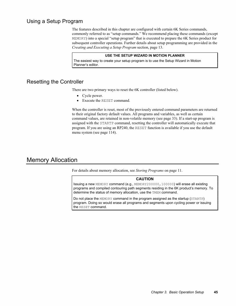
Chapter 3. Basic Operation Setup 45
Using a Setup Program The features described in this chapter are configured with certain 6K Series commands, commonly referred to as “setup commands.” We recommend placing these commands (except MEMORY) into a special “setup program” that is executed to prepare the 6K Series product for subsequent controller operations. Further details about setup programming are provided in the Creating and Executing a Setup Program section, page 13.
USE THE SETUP WIZARD IN MOTION PLANNER The easiest way to create your setup program is to use the Setup Wizard in Motion Planner’s editor.
Resetting the Controller There are two primary ways to reset the 6K controller (listed below).
• Cycle power. • Execute the RESET command.
When the controller is reset, most of the previously entered command parameters are returned to their original factory default values. All programs and variables, as well as certain command values, are retained in non-volatile memory (see page 33). If a start-up program is assigned with the STARTP command, resetting the controller will automatically execute that program. If you are using an RP240, the RESET function is available if you use the default menu system (see page 114).
Memory Allocation For details about memory allocation, see Storing Programs on page 11.
CAUTION Issuing a new MEMORY command (e.g., MEMORY200000,100000) will erase all existing programs and compiled contouring path segments residing in the 6K product’s memory. To determine the status of memory allocation, use the TMEM command.
Do not place the MEMORY command in the program assigned as the startup (STARTP) program. Doing so would erase all programs and segments upon cycling power or issuing the RESET command.

46 6K Series Programmer’s Guide
Drive Setup
Drive Type Selection 6K products can control any combination of stepper and servo axes. To tell the 6K which type of drive you are using and a particular axis, use the AXSDEF command. Stepper drives receive their positioning information via step and direction signals. Servo drives receive their positioning commands via a ±10 volt signal.
NOTE: If a drive is attached at the time you issue the AXSDEF command, the drive must be disabled (DRIVE0).
Make your drive type selection before configuring other parameters that are relative to the drive type.
The value of AXSDEF disables command fields that are not appropriate for that type of drive. For example, an axis configured as a stepper cannot be affected by a Servo Proportional Gain (SGP) command. The report back of non-applicable commands contains “-” in the field for that axis.
AXSDEF0 — Stepper Only Commands: DRES FMAXA ENCCNT FMAXV ESDB PULSE ESK ESTALL
AXSDEF1 — Servo Only Commands: ANIFB DSTALL KDRIVE PER SFB SGP SGI SGV SGVF SGAF SGILIM SOFFS SMPER SGSET SGENB STRGTD STRGTE STRGTT STRGTV TFB TGAIN TPER TSGSET TSTLT
Drive Fault Input Enable the Drive Fault Input
Use the DRFEN command to enable or disable checking the state of the drive fault input for each axis. The default condition is that the drive fault input is not checked (DRFEN0); therefore, a drive fault would not be detectable. Even with DRFEN enabled (DRFEN1), the controller will not respond to a drive fault condition until the respective axis is enabled with the DRIVE1 command. The drive fault input must be enabled (DRFEN1) before you can use these functions (remember that the default power-up state is disabled):
• AS, TAS, and TASF (axis status) bit 14 reports if a drive fault occurred. • ERROR bit 4 enables checking for the occurrence of a drive fault, and when is does, to
branch to the ERRORP program. • ER, TER, and TERF (error status) bit 4 reports if a drive fault occurred (if ERROR bit 4 is
enabled). • An output assigned the “Fault Indicator” function (OUTFNCi-F) will turn on when a
drive fault occurs or a user fault input (INFNCi-F or LIMFNCi-F) is activated.
Regardless of the state of the DRFEN command, the extended axis status bit 4 (reported with ASX, TASX, and TASXF) will accurately report the hardware state of the drive fault input.
Set the Drive Fault Input Active Level
The drive fault level (DRFLVL) should be set to “active high” or “active low” for each axis. The default setting is “active high” (DRFLVL1). The drive fault input schematic is shown in your 6K Series product installation guide. Use the table below as a guide.
Compumotor Product Drive Fault Level
GEMINI, APEX, Dynaserv, LN, OEM Series, S, TQ, ZETA ............Active High (DRFLVL1) SV, BLH, L, LE, PDS, PK130 ..........................................................Active Low (DRFLVLØ)
NOTE: If you are using a drive that does not have a drive fault output, set the drive fault level to active low (DRFLVLØ).
NOTE Once the drive fault level has been configured, you must enable the drive fault input with the DRFEN1 command before the input is usable.

Chapter 3. Basic Operation Setup 47
Checking Drive Fault Input Status (see table below): Axis status bit 14 (TASF, TAS or AS commands) indicates the drive fault input status, but only while the drive is enabled (DRIVE1) and the drive fault input is enabled (DRFEN1). If you need to monitor the drive fault input status regardless of the state of DRIVE and DRFEN, use the extended axis status bit 4 (TASXF, TASX, or ASX commands).
Drive Fault Level (DRFLVL)
Status of device driving the Fault input
Axis Status of Bit 14 (or) Extended Axis Status Bit 4
DRFLVL1 (active high)
OFF or not connected (not sinking current) ON (sinking current)
1 (drive fault has occurred) Ø
DRFLVLØ (active low)
OFF or not connected (not sinking current) ON (sinking current)
Ø 1 (drive fault has occurred)
When a drive fault occurs, motion will be stopped on all axes (stopped at the LHAD & LHADA deceleration values) and program execution will be terminated.
Drive Stall Detection (stepper axes only) The DSTALL command determines if the Stall Input on pin 4 of the DRIVE connector will be checked as Drive Stall indicator.
The state of the Stall Input can be monitored at all times with Extended Axis Status bit 7 (reported with TASX, TASF, and the ASX assignment/comparison operand); if left unconnected, the input is low, and status bit 7 will be set (reports a “1”). If this input is enabled as a drive stall indicator with the DSTALL1 command, a low input will be interpreted as a Drive Stall.
When a Drive Stall is detected, the 6K responds as follows: (this response is the same as that for Encoder Stall Detection, which is enabled with the ESTALL command)
• The stall is reported with Axis Status bit 12 (reported with TAS, TASF, and AS). • If ERROR error-checking bit 1 is enabled (ERROR.1-1):
- The stall is reported with Error Status bit 1 (reported with TER, TERF, and ER). - The 6K branches to the assigned ERRORP program.
• If the Kill-on-Stall feature is enabled (ESK1), the 6K immediately stops pulses from being sent to the affected axis.
Drive Resolution (stepper axes only) The drive resolution controls the number of steps the 6K controller considers as a full revolution for the motor drive. The controller's resolution is set with the DRES command (default is 4,000 steps/rev). Refer to the user documentation that accompanied your drive if you need to change its resolution.
IMPORTANT!
If the controller's resolution (set with the DRES command) does not match the drive's resolution, the motor will not move according to the programmed distance and velocity.
Step Pulse (stepper axes only) The step output pulse width can be varied using the PULSE command. The pulse width can be 0.3 µs to 8 µs (default is 0.3 µs). The pulse width is the amount of time the step output signal is active (see illustration below). The step output pulse width should be configured to meet the minimum step input pulse width requirement of the motor drive you are using.
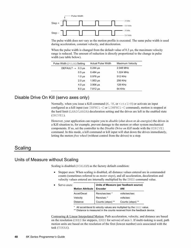
48 6K Series Programmer’s Guide
Step -
Step +
Pulse Width
0.4 Volts
4 Volts
0.4 Volts
4 Volts
The pulse width does not vary as the motion profile is executed. The same pulse width is used during acceleration, constant velocity, and deceleration.
When the pulse width is changed from the default value of 0.3 µs, the maximum velocity range is reduced. The amount of reduction is directly proportional to the change in pulse width (see table below).
Pulse Width (PULSE) Setting Actual Pulse Width Maximum Velocity
DEFAULT → 0.3 µs 0.244 µs 2.048 MHz
0.5 µs 0.484 µs 1.024 MHz 1.0 µs 0.976 µs 512 KHz 2.0 µs 1.953 µs 256 KHz 4.0 µs 3.906 µs 128 KHz 8.0 µs 7.812 µs 64 KHz
Disable Drive On Kill (servo axes only) Normally, when you issue a Kill command (K, !K, or <ctrl>K) or activate an input configured as a kill input (see INFNCi-C or LIMFNCi-C command), motion is stopped at the hard limit (LHAD/LHADA) deceleration setting and the drives are left in the enabled state (DRIVE1).
However, your application can require you to disable (shut down or de-energize) the drives in a Kill situation to, for example, prevent damage to the motors or other system mechanical components. If so, set the controller to the Disable Drive on Kill mode with the KDRIVE1 command. In this mode, a kill command or kill input will shut down the drives immediately, letting the motors free wheel (without control from the drives) to a stop.
Scaling
Units of Measure without Scaling Scaling is disabled (SCALEØ) as the factory default condition:
• Stepper axes: When scaling is disabled, all distance values entered are in commanded counts (sometimes referred to as motor steps), and all acceleration, deceleration and velocity values entered are internally multiplied by the DRES command value.
• Servo axes: Units of Measure (per feedback source) Motion Attribute Encoder ANI
Accel/Decel Revs/sec/sec * volts/sec/sec Velocity Revs/sec * volts/sec Distance Counts (steps) ** Counts (steps) **
* All accel/decel & velocity values are multiplied by the ERES value. ** Distance is measured in the counts received from the feedback device.
Contouring & Linear Interpolated Motion: Path acceleration, velocity, and distance are based on the resolution (DRES for steppers, ERES for servos) of axis 1. If multi-tasking is used, path motion units are based on the resolution of the first (lowest number) axis associated with the task (TSKAX).

Chapter 3. Basic Operation Setup 49
What is Scaling? Scaling allows you to program acceleration, deceleration, velocity, and position values in units of measure that are appropriate for your application. The SCALE command is used to enable or disable scaling (SCALE1 to enable, SCALEØ to disable). The motion type(s) you are using in your application determines which scale factor commands you need to configure:
Type of Motion
Accel/Decel Scaling
Velocity Scaling
Distance Scaling
Standard Point-to-Point Motion SCLA SCLV SCLD
Following SCLA SCLV SCLD for follower distances SCLMAS for master distances
Contouring, Linear Interpolation SCLD (used for all path motion scaling)
When Should I Define Scaling Factors?
NOTE All scaling parameters are saved in battery-backed RAM
Scaling calculations are performed when a program is defined or downloaded. Consequently, you must enable scaling (SCALE1) and define the scaling factors (SCLD, SCLA, SCLV, SCLMAS) prior to defining (DEF), uploading (TPROG), or running (RUN) the program.
RECOMMENDATION: Place the scaling commands at the beginning of your program file, before the location of any defined programs. This ensures that the motion parameters in subsequent programs in your program file are scaled correctly. When you use Motion Planner’s Setup Generator wizard, the scaling commands are automatically placed in the appropriate location in your program file.
ALTERNATIVE: Scaling factors could be defined via a terminal emulator just before defining or downloading a program. Because scaling command values are saved in battery-backed RAM (remembered after you cycle power or issue a RESET command), all subsequent program definitions and downloads will be scaled correctly.
NOTES • Scaling commands are not allowed in a program. If there are scaling commands in a
program, the controller will report an error message (“COMMAND NOT ALLOWED IN PROGRAM”) when the program is downloaded.
• If you intend to upload a program with scaled motion parameters, be sure to use Motion Planner. Motion Planner automatically uploads the scaling parameters and places them at the beginning of the program file containing the uploaded program from the controller. This ensures correct scaling when the program file is later downloaded.
Servo Axes Scaling can be used with encoder or analog input feedback sources. When the scaling commands (SCLA, SCLD, etc.) are executed, they are specific only to the current feedback source selected with the last SFB command. If your application requires switching between feedback sources for the same axis, then for each feedback source, you must select the feedback source with the appropriate SFB command and issue the scaling factors specific to operating with that feedback source. For example, if you have two axes and will be switching between encoder and ANI feedback, you should include code similar to the following in your setup program: SFB1,1 ; Select encoder feedback (subsequent scaling ; parameters are specific to encoder feedback) SCLA4000,4000 ; Program accel/decel in revs/sec/sec SCLV4000,4000 ; Program velocity in revs/sec SCLD4000,4000 ; Program distances in revs SFB2,2 ; Select ANI feedback (subsequent scaling ; parameters are specific to ANI feedback) SCLA205,205 ; Program accel/decel in volts/sec/sec SCLV205,205 ; Program velocity in volts/sec SCLD205,205 ; Program distances in volts

50 6K Series Programmer’s Guide
Acceleration & Deceleration Scaling (SCLA) Stepper Axes: If scaling is enabled (SCALE1), all accel/decel values entered are internally
multiplied by the acceleration scaling factor to convert user units/sec/sec to commanded counts/sec/sec. The scaled values are always in reference in commanded counts, regardless of the existence of an encoder.
Servo Axes: If scaling is enabled (SCALE1), all accel/decel values entered are internally multiplied by the acceleration scaling factor to convert user units/sec/sec to encoder or analog input counts/sec/sec.
All accel/decel commands for point-to-point motion (e.g., A, AA, AD, HOMA, HOMAD, JOGA, etc.) are multiplied by the SCLA command value. NOTE: All accel/decel commands for linear interpolated and contouring motion (e.g., PA, PAD, etc.) are multiplied by the SCLD command value.
SCLA value (steps/unit2)
Decimal Places
As the accel/decel scaling factor (SCLA) changes, the resolution of the accel and decel values and the number of positions to the right of the decimal point also change (see table at right). An accel/decel value with greater resolution than allowed will be truncated (e.g., if scaling is set to SCLA10, the A9.9999 command would be truncated to A9.9).
1 - 9 10 - 99 100 - 999 1000 - 9999 10000 - 99999 100000 - 999999
0 1 2 3 4 5
Use the following equations to determine the range of acceleration and deceleration values for your product.
Axis Type Minimum Accel or Decel (resolution) Maximum Accel or Decel Stepper
SCLADRES 0.001∗
SCLADRES 999.9999∗
Servo Encoder feedback:
SCLAERES 0.001∗
ANI feedback: SCLA0.205
Encoder feedback: SCLA
ERES 999.9999∗
ANI feedback: SCLA
5204799.979
Velocity Scaling (SCLV) Stepper Axes: If scaling is enabled (SCALE1), all velocity values entered are internally
multiplied by the velocity scaling factor to convert user units/sec to commanded counts/sec. The scaled values are always in reference to commanded counts (sometimes referred to as “motor steps”).
Servo Axes: If scaling is enabled (SCALE1), all velocity values entered are internally multiplied by the velocity scaling factor to convert user units/sec to encoder or analog input counts/sec.
All velocity commands for point-to-point motion (e.g., V, HOMV, HOMVF, JOGVH, JOGVL, etc.) are multiplied by the SCLV command value. NOTE: The velocity commands for linear interpolated and contouring motion (PV and PVF) are multiplied by the SCLD command value.
As the velocity scaling factor (SCLV) changes, the velocity command's range and its decimal places also change (see table below). A velocity value with greater resolution than allowed will be truncated. For example, if scaling is set to SCLV10, the V9.9999 command would be truncated to V9.9.
If the analog input voltage range is changed, the equations will change. See ANIRNG command for details.
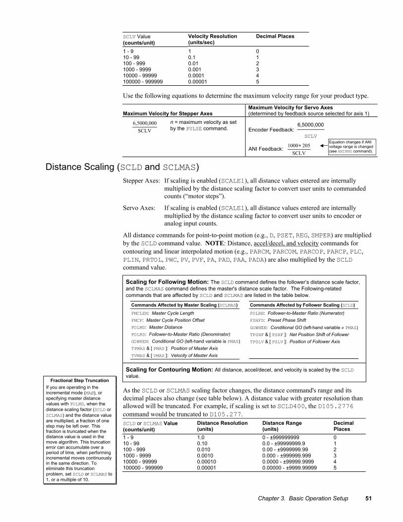
Chapter 3. Basic Operation Setup 51
SCLV Value (counts/unit)
Velocity Resolution (units/sec)
Decimal Places
1 - 9 10 - 99 100 - 999 1000 - 9999 10000 - 99999 100000 - 999999
1 0.1 0.01 0.001 0.0001 0.00001
0 1 2 3 4 5
Use the following equations to determine the maximum velocity range for your product type.
Maximum Velocity for Stepper Axes
Maximum Velocity for Servo Axes (determined by feedback source selected for axis 1)
SCLV6,5000,000
n = maximum velocity as set by the PULSE command. Encoder Feedback:
SCLV
6,5000,000
ANI Feedback: SCLV
205 1000 ∗
Distance Scaling (SCLD and SCLMAS) Stepper Axes: If scaling is enabled (SCALE1), all distance values entered are internally
multiplied by the distance scaling factor to convert user units to commanded counts (“motor steps”).
Servo Axes: If scaling is enabled (SCALE1), all distance values entered are internally multiplied by the distance scaling factor to convert user units to encoder or analog input counts.
All distance commands for point-to-point motion (e.g., D, PSET, REG, SMPER) are multiplied by the SCLD command value. NOTE: Distance, accel/decel, and velocity commands for contouring and linear interpolated motion (e.g., PARCM, PARCOM, PARCOP, PARCP, PLC, PLIN, PRTOL, PWC, PV, PVF, PA, PAD, PAA, PADA) are also multiplied by the SCLD command value.
Scaling for Following Motion: The SCLD command defines the follower’s distance scale factor, and the SCLMAS command defines the master's distance scale factor. The Following-related commands that are affected by SCLD and SCLMAS are listed in the table below. Commands Affected by Master Scaling (SCLMAS) Commands Affected by Follower Scaling (SCLD) FMCLEN: Master Cycle Length
FMCP: Master Cycle Position Offset FOLMD: Master Distance FOLRD: Follower-to-Master Ratio (Denominator) GOWHEN: Conditional GO (left-hand variable is PMAS) TPMAS & [ PMAS ]: Position of Master Axis TVMAS & [ VMAS ]: Velocity of Master Axis
FOLRN: Follower-to-Master Ratio (Numerator) FSHFD: Preset Phase Shift GOWHEN: Conditional GO (left-hand variable ≠ PMAS) TPSHF & [ PSHF ]: Net Position Shift of Follower TPSLV & [ PSLV ]: Position of Follower Axis
Scaling for Contouring Motion: All distance, accel/decel, and velocity is scaled by the SCLD value.
As the SCLD or SCLMAS scaling factor changes, the distance command's range and its decimal places also change (see table below). A distance value with greater resolution than allowed will be truncated. For example, if scaling is set to SCLD400, the D105.2776 command would be truncated to D105.277. SCLD or SCLMAS Value (counts/unit)
Distance Resolution (units)
Distance Range (units)
Decimal Places
1 - 9 1.0 0 - ±999999999 0 10 - 99 0.10 0.0 - ±99999999.9 1 100 - 999 0.010 0.00 - ±9999999.99 2 1000 - 9999 0.0010 0.000 - ±999999.999 3 10000 - 99999 0.00010 0.0000 - ±99999.9999 4 100000 - 999999 0.00001 0.00000 - ±9999.99999 5
Fractional Step Truncation
If you are operating in the incremental mode (MAØ), or specifying master distance values with FOLMD, when the distance scaling factor (SCLD or SCLMAS) and the distance value are multiplied, a fraction of one step may be left over. This fraction is truncated when the distance value is used in the move algorithm. This truncation error can accumulate over a period of time, when performing incremental moves continuously in the same direction. To eliminate this truncation problem, set SCLD or SCLMAS to 1, or a multiple of 10.
Equation changes if ANI voltage range is changed (see ANIRNG command).

52 6K Series Programmer’s Guide
Scaling Example — Stepper Axes
Axis 1 and axis 2 control 25,000 step/rev motor/drives attached to 5-pitch leadscrews. The user wants to program motion parameters in inches; therefore the scale factor calculation is: 25,000 steps/rev x 5 revs/inch = 125,000 steps/inch. For instance, with a scale factor of 125,000, the operator could enter a move distance value of 2.000 and the controller would send out 250,000 pulses, corresponding to two inches of travel. SCALE1 ; Enable scaling DRES25000,25000 ; Set drive resolution to 25,000 steps/rev on both axes SCLD125000,125000 ; Allow entering distance in inches (both axes) SCLV125000,125000 ; Allow entering velocity in inches/sec (both axes) SCLA125000,125000 ; Allow entering accel/decel in inches/sec/sec
Scaling Example — Servo Axes
Axis 1 controls a 4,000 count/rev servo motor/drive system (using a 1000-line encoder) attached to a 5-pitch leadscrew. The user wants to position in inches; therefore, the scale factor calculation is 4,000 counts/rev x 5 revs/inch = 20,000 counts/inch. Half way through the motion process, axis 1 must switch to ANI feedback for the purpose of positioning to a voltage (scale factor is 205 counts/volt).
Axis 2 controls a 4,000 count/rev servo motor/drive system (using a 1000-line encoder) attached to a 10-pitch leadscrew. The user wants to position in inches (scale factor calculation: 4,000 counts/rev x 10 revs/inch = 40,000 counts/inch). SFB1,1 ; Select encoder feedback for both axes ERES4000 ; Set encoder resolution to 4000 steps/rev (post quadrature) SCALE1 ; Enable scaling SCLD20000,40000 ; Allow entering distance values in inches SCLV20000,40000 ; Allow entering velocity values in inches/sec SCLA20000,40000 ; Allow entering accel/decel values in inches/sec/sec SFB2 ; Select ANI feedback for axis 1 SCALE1 ; Enable scaling SCLD205 ; Allow entering distance values in volts SCLV205 ; Allow entering velocity values in volts/sec SCLA205 ; Allow entering accel/decel values in volts/sec/sec SFB1,1 ; Select encoder feedback for both axes (prepare for motion)
Scaling Example — Following
Typically, the master and follower scale factors are programmed so that master and follower units are the same, but this is not required. Consider the scenario below as an example.
The master is a 1000-line encoder (4000 counts/rev post-quadrature) mounted to a 50 teeth/rev pulley attached to a 10 teeth/inch conveyor belt, resulting in 80 counts/tooth (4000 counts/50 teeth = 80 counts/tooth). To program in inches, you would set up the master scaling factor with the SCLMAS800 command (80 counts/tooth ∗ 10 teeth/inch = 800 counts/inch). The follower axis is a servo motor with position feedback from a 1000-line encoder (4000 counts/rev). The motor is mounted to a 4-pitch (4 revs/inch) leadscrew. Thus, to program in inches, you would set up the follower scaling factor with the SCLD16000 command (4000 counts/rev ∗ 4 revs/inch = 16000 counts/inch). SCALE1 ; Enable scaling SCLMAS800 ; Master scaling: ; (80 counts/tooth * 10 teeth/inch = 800 counts/inch) SCLD16000 ; Follower scaling:
; (4000 counts/rev 4 revs/inch = 16000 counts/inch) Scaling Example — Contouring and Linear Interpolation
This simple example uses 2 servo axes (axes 1 and 2) for contouring. Both axes use encoder feedback with a resolution (ERES) of 4000 counts/rev, axis 1 uses a 10-pitch (10 revs per inch) leadscrew and axis 2 uses a 5-pitch (5 revs per inch) lead screw, and you want to program in inches. For this application you would use the SCLD40000,20000 command to establish path motion units in inches: distance is inches, acceleration is inches/sec/sec, and velocity is inches/sec. NOTE that all path motion attributes are scaled by the SCLD value. SCALE1 ; Enable scaling SCLD40000,20000 ; Set scaling to program in inches: ; Axis 1: 4000 counts/rev * 10 revs/inch = 40000 counts/inch ; Axis 2: 4000 counts/rev * 5 revs/inch = 20000 counts/inch PV5 ; Set path velocity to 5 inches/sec PA50 ; Set path acceleration to 50 inches/sec/sec PAD100 ; Set path deceleration to 100 inches/sec/sec DEF prog1 ; Begin definition of path named prog1 PAXES1,2 ; Set axes 1 and 2 as the X and Y contouring axes PAB0 ; Set to incremental coordinates PLIN1,1 ; Specify X-Y endpoint position to create a 45 degree ; angle line segment END ; End definition of path prog1 PCOMP prog1 ; Compile path prog1 PRUN prog1 ; Execute path prog1

Chapter 3. Basic Operation Setup 53
Positioning Modes
But first, a word about basic motion… Accel, Decel, Velocity, Distance
The basic motion profile comprises acceleration, deceleration, velocity, and distance commands (see table below). Motion is generally initiated with the GO command.
Parameter Units (Unscaled), Stepper Units (Unscaled), Servo Unit Scaling Command *
Acceleration revs/sec2 encoder/resolver: revs/sec2 ANI: volts/sec2
SCLA (or SCLD **)
Deceleration revs/sec2 encoder/resolver: revs/sec2 ANI: volts/sec2
SCLA (or SCLD **)
Velocity revs/sec encoder/resolver: revs/sec ANI: volts/sec
SCLV (or SCLD **)
Distance steps counts SCLD ***
* Scaling must first be enabled with the SCALE1 command. For details on scaling, refer to page 48. ** All Contouring and linear interpolated motion is scaled with SCLD (distance, accel/decel, and velocity). *** An axis assigned as a master (for Following) is scaled by the SCLMAS command.
Example Program
Resulting Motion Profile: Velocity
Distance
V8
A20 A5
D100000
The program below controls two axes of motion. Axis 1 produces a preset (incremental) 100,000-count move in a nominally trapezoidal profile. Axis 2 produces a preset 80,000-count move in a nominally trapezoidal profile.
DEL BASIC ; Delete program called BASIC DEF BASIC ; Begin definition of program called BASIC MC00 ; Use the preset positioning mode for axes 1 & 2 MA00 ; Use the incremental (preset) positioning mode A20,10 ; Accelerate axis 1 at 20 revs/sec/sec, and axis 2 at 10 AD5,5 ; Decelerate axis 1 and axis 2 at 5 revs/sec/sec V8,5 ; Set axis 1 velocity to 8 revs/sec, and axis 2 to 5 D100000,80000 ; Set distance to 100,000 counts GO11 ; Execute the motion on both axes END ; End definition of BASIC
Axis 1 profile: Axis 2 profile:
Velocity
Distance
V8
A20 AD5
D100000
Velocity
Distance
A10 AD5
D80000
V5
Direction of Motion for Rotary Motors
Positive distance values (e.g., D20000) represent clockwise motion, negative values (e.g., D-20000) represent counter-clockwise motion. This assumes you connected the drive and motor (and feedback device for servo drives) according to the Hardware Installation Guide instructions. ��� ���%�&'���
� �����(���� ���
��&'���
�������(���� ���
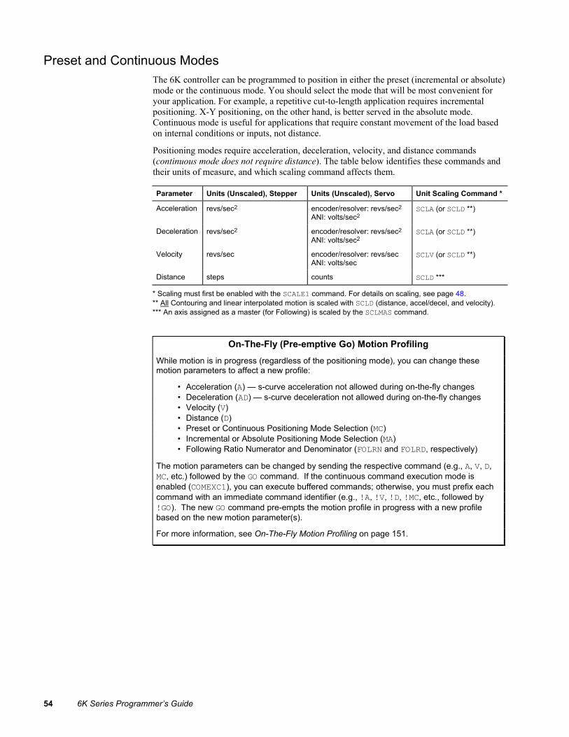
54 6K Series Programmer’s Guide
Preset and Continuous Modes The 6K controller can be programmed to position in either the preset (incremental or absolute) mode or the continuous mode. You should select the mode that will be most convenient for your application. For example, a repetitive cut-to-length application requires incremental positioning. X-Y positioning, on the other hand, is better served in the absolute mode. Continuous mode is useful for applications that require constant movement of the load based on internal conditions or inputs, not distance.
Positioning modes require acceleration, deceleration, velocity, and distance commands (continuous mode does not require distance). The table below identifies these commands and their units of measure, and which scaling command affects them.
Parameter Units (Unscaled), Stepper Units (Unscaled), Servo Unit Scaling Command *
Acceleration revs/sec2 encoder/resolver: revs/sec2 ANI: volts/sec2
SCLA (or SCLD **)
Deceleration revs/sec2 encoder/resolver: revs/sec2 ANI: volts/sec2
SCLA (or SCLD **)
Velocity revs/sec encoder/resolver: revs/sec ANI: volts/sec
SCLV (or SCLD **)
Distance steps counts SCLD ***
* Scaling must first be enabled with the SCALE1 command. For details on scaling, see page 48. ** All Contouring and linear interpolated motion is scaled with SCLD (distance, accel/decel, and velocity). *** An axis assigned as a master (for Following) is scaled by the SCLMAS command.
On-The-Fly (Pre-emptive Go) Motion Profiling While motion is in progress (regardless of the positioning mode), you can change these motion parameters to affect a new profile:
• Acceleration (A) — s-curve acceleration not allowed during on-the-fly changes • Deceleration (AD) — s-curve deceleration not allowed during on-the-fly changes • Velocity (V) • Distance (D) • Preset or Continuous Positioning Mode Selection (MC) • Incremental or Absolute Positioning Mode Selection (MA) • Following Ratio Numerator and Denominator (FOLRN and FOLRD, respectively)
The motion parameters can be changed by sending the respective command (e.g., A, V, D, MC, etc.) followed by the GO command. If the continuous command execution mode is enabled (COMEXC1), you can execute buffered commands; otherwise, you must prefix each command with an immediate command identifier (e.g., !A, !V, !D, !MC, etc., followed by !GO). The new GO command pre-empts the motion profile in progress with a new profile based on the new motion parameter(s).
For more information, see On-The-Fly Motion Profiling on page 151.
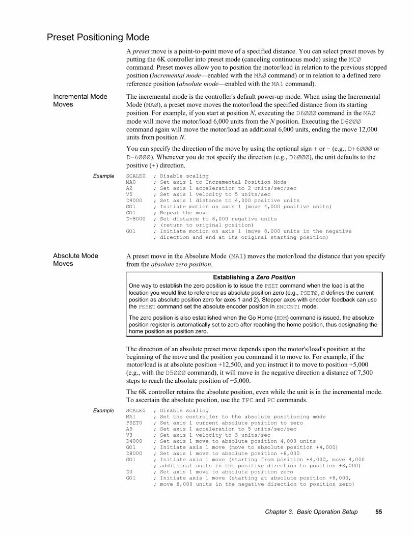
Chapter 3. Basic Operation Setup 55
Preset Positioning Mode A preset move is a point-to-point move of a specified distance. You can select preset moves by putting the 6K controller into preset mode (canceling continuous mode) using the MCØ command. Preset moves allow you to position the motor/load in relation to the previous stopped position (incremental mode—enabled with the MAØ command) or in relation to a defined zero reference position (absolute mode—enabled with the MA1 command).
Incremental Mode Moves
The incremental mode is the controller's default power-up mode. When using the Incremental Mode (MAØ), a preset move moves the motor/load the specified distance from its starting position. For example, if you start at position N, executing the D6ØØØ command in the MAØ mode will move the motor/load 6,000 units from the N position. Executing the D6ØØØ command again will move the motor/load an additional 6,000 units, ending the move 12,000 units from position N.
You can specify the direction of the move by using the optional sign + or - (e.g., D+6ØØØ or D-6ØØØ). Whenever you do not specify the direction (e.g., D6ØØØ), the unit defaults to the positive (+) direction.
Example SCALE0 ; Disable scaling MA0 ; Set axis 1 to Incremental Position Mode A2 ; Set axis 1 acceleration to 2 units/sec/sec V5 ; Set axis 1 velocity to 5 units/sec D4000 ; Set axis 1 distance to 4,000 positive units GO1 ; Initiate motion on axis 1 (move 4,000 positive units) GO1 ; Repeat the move D-8000 ; Set distance to 8,000 negative units ; (return to original position) GO1 ; Initiate motion on axis 1 (move 8,000 units in the negative ; direction and end at its original starting position)
Absolute Mode Moves
A preset move in the Absolute Mode (MA1) moves the motor/load the distance that you specify from the absolute zero position.
Establishing a Zero Position One way to establish the zero position is to issue the PSET command when the load is at the location you would like to reference as absolute position zero (e.g., PSETØ,Ø defines the current position as absolute position zero for axes 1 and 2). Stepper axes with encoder feedback can use the PESET command set the absolute encoder position in ENCCNT1 mode.
The zero position is also established when the Go Home (HOM) command is issued, the absolute position register is automatically set to zero after reaching the home position, thus designating the home position as position zero.
The direction of an absolute preset move depends upon the motor's/load's position at the beginning of the move and the position you command it to move to. For example, if the motor/load is at absolute position +12,500, and you instruct it to move to position +5,000 (e.g., with the D5ØØØ command), it will move in the negative direction a distance of 7,500 steps to reach the absolute position of +5,000.
The 6K controller retains the absolute position, even while the unit is in the incremental mode. To ascertain the absolute position, use the TPC and PC commands.
Example SCALE0 ; Disable scaling MA1 ; Set the controller to the absolute positioning mode PSET0 ; Set axis 1 current absolute position to zero A5 ; Set axis 1 acceleration to 5 units/sec/sec V3 ; Set axis 1 velocity to 3 units/sec D4000 ; Set axis 1 move to absolute position 4,000 units GO1 ; Initiate axis 1 move (move to absolute position +4,000) D8000 ; Set axis 1 move to absolute position +8,000 GO1 ; Initiate axis 1 move (starting from position +4,000, move 4,000 ; additional units in the positive direction to position +8,000) D0 ; Set axis 1 move to absolute position zero GO1 ; Initiate axis 1 move (starting at absolute position +8,000, ; move 8,000 units in the negative direction to position zero)

56 6K Series Programmer’s Guide
Continuous Positioning Mode The Continuous Mode (MC1) is useful in these situations:
• Applications that require constant movement of the load • Synchronize the motor to external events such as trigger input signals • Changing the motion profile after a specified distance or after a specified time period
(T command) has elapsed
You can manipulate the motor movement with either buffered or immediate commands. After you issue the GO command, buffered commands are not executed unless the continuous command execution mode (COMEXC1 command) is enabled. Once COMEXC1 is enabled, buffered commands are executed in the order in which they were programmed. More information on the COMEXC mode is provided on page 15.
The command can be specified as immediate by placing an exclamation mark (!) in front of the command. When a command is specified as immediate, it is placed at the front of the command queue and is executed immediately.
Example A COMEXC1 ; Enable continuous command processing mode COMEXS1 ; Allow command execution to continue after stop MC1 ; Sets axis 1 mode to continuous A10 ; Sets axis 1 acceleration to 10 V1 ; Sets axis 1 velocity to 1 GO1 ; Initiates axis 1 move (Go) WAIT(1VEL=1) ; Wait to reach continuous velocity T5 ; Time delay of 5 seconds S1 ; Initiate stop of axis 1 move WAIT(MOV=b0) ; Wait for motion to completely stop on axis 1 COMEXC0 ; Disable continuous command processing mode ; When the move is executed, the load will accelerate to 1 unit/sec, ; continue at that rate for 5 seconds, and then decelerate to a stop.
Example B DEF prog1 ; Begin definition of program prog1 COMEXC1 ; Enable continuous command processing mode COMEXS1 ; Allow command execution to continue after stop MC1 ; Set axis 1 to continuous positioning mode A10 ; Set axis 1 acceleration to 10 V1 ; Set axis 1 velocity to 1 GO1 ; Initiate axis 1 move (Go) WAIT(1VEL=1) ; Wait for motor to reach continuous velocity T3 ; Time delay of 3 seconds A50 ; Set axis 1 acceleration to 50 V10 ; Set axis 1 velocity to 10 GO1 ; Initiate acceleration and velocity changes on axis 1 T5 ; Time delay of 5 seconds S1 ; Initiate stop of axis 1 move WAIT(MOV=b0) ; Wait for motion to completely stop on axis 1 COMEXC0 ; Disable continuous command processing mode END ; End definition of program prog1
While in continuous mode, motion can be stopped if: • You issue an immediate Stop (!S) or Kill (!K or ctrl/K) command. • The load trips an end-of-travel limit switch or encounters a software end-of-travel limit. • The load trips a registration input (a trigger input configured with the INFNCi-H
command to function as a registration input). • The load trips an input configured as a kill input (INFNCi-C or LIMFNCi-C) or a
stop input (INFNCi-D or LIMFNCi-D).
NOTE While the axis is moving, you cannot change the parameters of some commands (such as DRIVE and HOM). This rule applies during the COMEXC1 mode and even if you prefix the command with an immediate command identifier (!). For more information, see Restricted Commands During Motion on page 17.

Chapter 3. Basic Operation Setup 57
End-of-Travel Limits
Related Commands
LH .............Hard limit enable LHAD .........Hard limit decel LHADA .......Hard limit decel (s) LIMLVL .....Limit switch polarity LS .............Soft limit enable LSAD .........Soft limit decel LSADA .......Soft limit decel (s) LSNEG .......Soft limit (negative) LSPOS .......Soft limit (positive) TLIM .........Hard limit status TASF .........Bits 15-18 indicate if ..................hard or soft limit ..................was encountered TERF .........Bit 2: hard limit hit ..................Bit 3: soft limit hit ..................(must enable ERROR ..................checking bits 2 & 3) ERROR .......Bit 2 or 3 is enabled, ..................the 6K will branch to ..................the ERRORP program ..................if a hard or soft limit ..................is encountered
The 6K controller can respond to both hardware and software end-of-travel limits. The purpose of hardware and software end-of-travel limits is to prevent the motor’s load from traveling past defined limits. Software and hardware limits are typically positioned in such a way that when the software limit is reached, the motor/load will start to decelerate toward the hardware limit, thus allowing for a much smoother stop at the hardware limit. Software limits can be used regardless of incremental or absolute positioning. When a hardware or software end-of-travel limit is reached, the 6K controller stops that axis using the respective hardware deceleration rate (set with LHAD & LHADA) or software limit deceleration rate (set with LSAD & LSADA).
How to set up hardware end-of-travel limits (for each axis):
1. Connect the end-of-travel limit inputs according to the instructions in your 6K product’s Installation Guide. To help assure safety, connect normally-closed switches and leave the active level at default “active low” setting (set with the LIMLVL command).
2. (Optional) Define the inputs to be used as end-of-travel inputs for the respective axes. NOTE: When the 6K product is shipped from the factory, the inputs on the “LIMITS/HOME” connectors are factory-configured with the LIMFNC command to function as end-of-travel and home limits for their respective axes. If you intend to use digital inputs on an external I/O brick as limit inputs:
a. Assign the limit function to the external input with the INFNC command. For example, 1INFNC9-1R assigns the “axis 1 positive end-of-travel limit” function to the 1st input on SIM2 (I/O point 9) of I/O brick 1.
b. Reassign the respective “LIMITS/HOME” input to a non-limit function with the LIMFNC command. For example, LIMFNC1-A assigns the “general-purpose input” function to limit input 1 (normally assigned the “axis 1 positive end-of- travel limit” function).
3. Set the hard limit deceleration rate (LHAD & LHADA) to be used when the limit switch is activated. The LHADA command allows you to define an s-curve deceleration. Stepper Axes: If your system is moving heavy loads or operating at high velocities, you can need to decrease the LHAD command value (deceleration rate) to prevent the motor from stalling (GEMINI and ZETA drives can compensate without reducing decel).
NOTES ON HARDWARE LIMITS • 6K controllers are shipped from the factory with the hardware end-of-travel limits
enabled, but not connected. Therefore, motion will not be allowed until you do one of the following:
- Install limit switches or jumper the end-of-travel limit terminals to the GND terminal (see your product's Installation Guide for wiring instructions).
- Disable the limits with the LH command (recommended only if the load is not coupled).
- Reverse the active level of the limits by executing the LIMLVL0 command for the respective axis.
• If you reverse the commanded direction polarity (CMDDIR1), you should swap the hardware end-of-travel switch connections to maintain a positive correlation with the commanded direction.

58 6K Series Programmer’s Guide
How to set up software end-of-travel limits (for each axis):
1. Use the LS command to enable the software end-of-travel limits for the appropriate axes (for example, LS1111 enables software limits for axes 1-4).
2. Define the positive-direction limit with the LSPOS command, and define the negative-direction limit with the LSNEG command. If you have scaling enabled (SCALE1), these limit values are scaled by the SCLD command. Both software limits can be defined with positive values (e.g., axis 2 in the example below)
NOTES ON SOFTWARE LIMITS • The software limits (LSPOS & LSNEG) are referenced from a position of absolute
zero. or negative values. Care must be taken when performing incremental moves because the software limits are always defined in absolute terms. They must be large enough to accommodate the moves, or a new zero reference position must be defined (using the PSET command) before each move.
• To ensure proper motion when using soft end-of-travel limits, be sure to set the LSPOS value to an absolute value greater than the LSNEG value.
Programming Example
In this sample of code (not a complete program), the hardware and software limits are enabled on axes 1 and 2, and disabled on axes 3 and 4. The distance scaling command (SCLD) is used to define software limit locations in revolutions from the absolute zero position (assumes a 4000 step/rev resolution). Deceleration rates are specified for both software and hardware limits. If a limit is encountered, the motors will decelerate to a stop. ; ********************************************************* ; These scaling setup commands are downloaded before the ; limit setup commands are executed: SCALE1 ; Enable scaling @SCLD4000 ; Program soft limit distance in revs (all axes) @SCLA4000 ; Program soft limit accel/decel in revs/sec/sec (all axes) @ERES4000 ; Set encoder resolution to 4000 steps/rev (all axes) ; ********************************************************* LH3,3,0,0 ; Enable limits 1 and 2, disable limits 3 and 4 LHAD10,10 ; Set hard limit deceleration LSAD5,10 ; Set soft limit deceleration LSNEG0,2 ; Set negative direction soft limit
; (axis 1: 0 revs; axis2: 2 revs) LSPOS10,20 ; Establish positive soft limit
; (axis 1: 10 revs; axis 1: 20 revs) LS3,3,0,0 ; Enable soft limits 1 and 2, disable limits 3 and 4

Chapter 3. Basic Operation Setup 59
Homing (Using the Home Inputs) Refer to the product's Installation Guide for instructions to wire hardware home limit switches.
The homing operation is a sequence of moves that position an axis using the Home Limit input and/or the Z Channel input of an incremental encoder. The goal of the homing operation is to return the load to a repeatable initial starting location.
Zero Reference After Homing: As soon as the homing operation is successfully completed, the absolute position register is reset to zero, thus establishing a zero reference position (for servo axes using analog input feedback, this applies also to the voltage register).
The homing operation has several potential homing functions you can customize to suit the needs of your application (illustrations of the effects of these commands are presented below):
Command Homing Function (see respective command descriptions for further details) Default HOM ...............Initiate the homing move. To start the homing move in the positive
direction, use HOMØ; to home in the negative direction, use HOM1. HOMx (do not home)
HOMA .............Acceleration while homing. HOMA1Ø (10 units/sec2)
HOMAA...........S-curve acceleration while homing. HOMAA10 (10 units/sec2)
HOMAD...........Deceleration while homing. HOMAD10 (10 units/sec2)
HOMADA.........S-curve deceleration while homing. HOMADA10 (10 units/sec2)
HOMBAC.........Back up to home. The load will decelerate to a stop after encountering the active edge of the home region, and then will move in the opposite direction at the HOMVF velocity until the active edge of the home region is encountered. Allows the use of HOMEDG and HOMDF.
HOMBAC0 (function disabled)
HOMDF...........Final approach direction —during backup to home (HOMBAC) or during homing to the Z channel input of an incremental encoder (HOMZ).
HOMDF0 (positive direction)
HOMEDG.........Specify the side of the home switch on which to stop (either the positive-travel side or the negative-travel side).
HOMEGD0 (positive-travel side of switch)
LIMLVL.........Define the home limit input active level (i.e., the state, high or low, which is to be considered an activation of the input). To use a normally-open switch, select active low (LIMLVL0); to use a normally-closed switch, select active high (LIMLVL1).
LIMLVL0 (active-low, use a normally-open switch)
HOMV .............Velocity while seeking the home position (see also HOMVF). HOMV1 (1 unit/sec)
HOMVF...........Velocity while in final approach to home position—during backup to home (HOMBAC) or during homing to the Z channel input of an incremental encoder (HOMZ).
HOMVF.1 (0.1 unit/sec)
HOMZ .............Home to the Z channel input from an incremental encoder. NOTE: The home limit input must be active prior to homing to the Z channel.
HOMZ0 (function disabled)
NOTES ABOUT HOMING
• Avoid using pause and resume functions during the homing operation. A pause command (PS or !PS) or pause/continue input (input configured with the INFNCi-E or LIMFNCi-E command) will pause the homing motion. However, when the subsequent resume command (C or !C) or pause/continue input occurs, motion will resume at the beginning of the homing motion sequence.
• Relevance of positive and negative direction:
)�����'���!��(��*����
+�����(��,������
- �%��%.��(��$����
������(��,������
- �%��%.��(��$����
+�����(��,������
-�������)���
������(��,������
-�������)���
• If an end-of-travel limit is encountered during the homing operation, the motion will be
reversed and the home switch will be sought in the opposite direction. If a second limit is encountered, the homing operation will be terminated, stopping motion at the second limit.
Homing Status: Status of homing moves is stored in bit #5 of the axis status register (indicates whether or not the home operation was successful). To display the status, use the TASF command or the TAS command. To use the status in a conditional expression (e.g., for an IF statement), use the AS assignment/com-parison operator.

60 6K Series Programmer’s Guide
Figures A and B show the homing operation when HOMBAC is not enabled. “CW” refers to the positive direction and “CCW” refers to the negative direction.
Figure A:
��/�-������)���
)����!��(�*����
�/�-������)���
0�����
��/$����
# �����������
�/$����
�������
Home Profile Attributes (commands): • Start home move in positive
direction (HOM0) • Backup To Home disabled
(HOMBAC0)
Figure B:
��/�-������)���
)����!��(�*����
�/�-������)���
0�����
��/$����
# �����������
�/$����
�������
Home Profile Attributes (commands): • Start home move in negative
direction (HOM1) • Backup To Home disabled
(HOMBAC0)
Positive Homing, Backup to Home Enabled
The seven steps below describe a sample homing operation when HOMBAC is enabled (see Figure C). The final approach direction (HOMDF) is CW and the home edge (HOMEDG) is the CW edge. “CW” refers to the positive direction and “CCW” refers to the negative direction.
NOTE To better illustrate the direction changes in the backup-to-home operation, the illustrations in the remainder of this section show the backup-to-home movements with varied velocities. In reality, the backup-to-home movements are performed at the same velocity (HOMVF value).
Step 1 A CW home move is started with the HOMØ command at the HOMA and HOMAA accelerations. Default HOMA is 10 revs (or volts or inches) per sec2.
Step 2 The HOMV velocity is reached (move continues at that velocity until home input goes active).
Step 3 The CCW edge of the home input is detected, this means the home input is active. At this time the move is decelerated at the HOMAD and HOMADA command values. It does not matter if the home input becomes inactive during this deceleration.
Step 4 After stopping, the direction is reversed and a second move with a peak velocity specified by the HOMVF value is started.
Step 5 This move continues until the CCW edge of the home input is reached. Step 6 Upon reaching the CCW edge, the move is decelerated at the HOMAD and HOMADA
command values, the direction is reversed, and another move is started in the CW direction at the HOMVF velocity.
Step 7 As soon as the home input CW edge is reached, this last move is immediately terminated. The load is at home and the absolute position register is reset to zero.

Chapter 3. Basic Operation Setup 61
Figure C:
��/�-������)���
)����!��(�*����
�/�-������)���
0�����
��/$����
# �����������
�/$����
�������
Home Profile Attributes (commands): • Start home move in positive
direction (HOM0) • Backup To Home enabled
(HOMBAC1) • Final approach direction is
positive (HOMDF0) • Stop on the positive-travel side
of the home switch active region (HOMEDG0)
Figures D through F show the homing operation for different values of HOMDF and HOMEDG, when HOMBAC is enabled. “CW” refers to the positive direction and “CCW” refers to the negative direction.
Figure D:
��/�-������)���
)����!��(�*����
�/�-������)���
0�����
��/$����
# �����������
�/$����
�������
Home Profile Attributes (commands): • Start home move in positive
direction (HOM0) • Backup To Home enabled
(HOMBAC1) • Final approach direction is
positive (HOMDF0) • Stop on the negative-travel side
of the home switch active region (HOMEDG1)
Figure E:
��/�-������)���
)����!��(�*����
�/�-������)���
0�����
��/$����
# �����������
�/$����
�������
Home Profile Attributes (commands): • Start home move in positive
direction (HOM0) • Backup To Home enabled
(HOMBAC1) • Final approach direction is
negative (HOMDF1) • Stop on the positive-travel side
of the home switch active region (HOMEDG0)
Figure F:
��/�-������)���
)����!��(�*����
�/�-������)���
0�����
��/$����
# �����������
�/$����
�������
Home Profile Attributes (commands): • Start home move in positive
direction (HOM0) • Backup To Home enabled
(HOMBAC1) • Final approach direction is
negative (HOMDF1) • Stop on the negative-travel side
of the home switch active region (HOMEDG1)

62 6K Series Programmer’s Guide
Negative Homing, Backup to Home Enabled
Figures G through J show the homing operation for different values of HOMDF and HOMEDG, when HOMBAC is enabled. “CW” refers to the positive direction and “CCW” refers to the negative direction.
Figure G:
��/�-������)���
)����!��(�*����
�/�-������)���
0�����
��/$����
# �����������
�/$����
�������
Home Profile Attributes (commands): • Start home move in negative
direction (HOM1) • Backup To Home enabled
(HOMBAC1) • Final approach direction is negative
(HOMDF1) • Stop on the negative-travel side of
the home switch active region (HOMEDG1)
Figure H:
��/�-������)���
)����!��(�*����
�/�-������)���
0�����
��/$����
# �����������
�/$����
�������
Home Profile Attributes (commands): • Start home move in negative
direction (HOM1) • Backup To Home enabled
(HOMBAC1) • Final approach direction is negative
(HOMDF1) • Stop on the positive-travel side of
the home switch active region (HOMEDG0)
Figure I:
��/�-������)���
)����!��(�*����
�/�-������)���
0�����
��/$����
# �����������
�/$����
�������
Home Profile Attributes (commands): • Start home move in negative
direction (HOM1) • Backup To Home enabled
(HOMBAC1) • Final approach direction is positive
(HOMDF0) • Stop on the negative-travel side of
the home switch active region (HOMEDG1)
Figure J:
��/�-������)���
)����!��(�*����
�/�-������)���
0�����
��/$����
# �����������
�/$����
�������
Home Profile Attributes (commands): • Start home move in negative
direction (HOM1) • Backup To Home enabled
(HOMBAC1) • Final approach direction is positive
(HOMDF0) • Stop on the positive-travel side of
the home switch active region (HOMEDG0)

Chapter 3. Basic Operation Setup 63
Homing Using The Z-Channel
Figures K through O show the homing operation when homing to an encoder index pulse, or Z channel, is enabled (HOMZ1). The Z-channel will only be recognized after the home input is activated. It is desirable to position the Z channel within the home active region; this reduces the time required to search for the Z channel. “CW” refers to the positive direction and “CCW” refers to the negative direction.
Figure K: 1���� �
!��(��*����
��/�-������)���
)����!��(�*����
�/�-������)���
0�����
��/$����
# �����������
�/$����
�������
Home Profile Attributes (commands): • Z-Channel homing enabled (HOMZ1) • Start home move in negative direction
(HOM1) • Backup To Home enabled (HOMBAC1) • Final approach direction is negative
(HOMDF1) • Stop on the negative-travel side of the
z-channel active region (HOMEDG1)
Figure L: 1���� �
!��(��*����
��/�-������)���
)����!��(�*����
�/�-������)���
0�����
��/$����
# �����������
�/$����
�������
Home Profile Attributes (commands): • Z-Channel homing enabled (HOMZ1) • Start home move in negative direction
(HOM1) • Backup To Home enabled (HOMBAC1) • Final approach direction is positive
(HOMDF0) • Stop on the positive-travel side of the
z-channel active region (HOMEDG0)
Figure M: 1���� �
!��(��*����
��/�-������)���
)����!��(�*����
�/�-������)���
0�����
��/$����
# �����������
�/$����
�������
Home Profile Attributes (commands): • Z-Channel homing enabled (HOMZ1) • Start home move in negative direction
(HOM1) • Backup To Home enabled (HOMBAC1) • Final approach direction is positive
(HOMDF0) • Stop on the positive-travel side of the
z-channel active region (HOMEDG0)
Figure N: 1���� �
!��(��*����
��/�-������)���
)����!��(�*����
�/�-������)���
0�����
��/$����
# �����������
�/$����
�������
Home Profile Attributes (commands): • Z-Channel homing enabled (HOMZ1) • Start home move in positive direction
(HOM0) • Backup To Home disabled (HOMBAC0) • Final approach direction is positive
(HOMDF0) • Stop on the positive-travel side of the
z-channel active region (HOMEDG0)
Figure O: 1���� �
!��(��*����
��/�-������)���
)����!��(�*����
�/�-������)���
0�����
��/$����
# �����������
�/$����
�������
Home Profile Attributes (commands): • Z-Channel homing enabled (HOMZ1) • Start home move in positive direction
(HOM0) • Backup To Home enabled (HOMBAC1) • Final approach direction is positive
(HOMDF0) • Stop on the positive-travel side of the
z-channel active region (HOMEDG0)

64 6K Series Programmer’s Guide
Encoder-Based Stepper Operation (stepper axes only) When using an encoder in an stepper application, you can configure the following:
• Encoder resolution • Stall Detection & Kill-on-Stall, Stall Deadband • Encoder polarity • Encoder-based position reference and position capture • Encoder failure detection • Commanded direction polarity
Encoder Resolution You must specify the encoder resolution with the ERES command. The power-up default value for encoder resolution is 4,000 counts/rev. Listed below are the resolution values for Compumotor-supplied encoders.
• -RE, -RC, -EC, and -E Series Encoders:...............ERES4000 • -HJ Series Encoders:.............................................ERES2048 • Daedal Positioning Tables (encoder options):
-E2 .........................ERES42000 -E3 .........................ERES84000 -E4 .........................ERES420000 -E5 .........................ERES8400
• Dynaserv: DR10xxB...............ERES507904 DR5xxxA.................ERES425894 DR1xxxE ...............ERES614400 DM10xxB................ERES655360 DR1xxxA...............ERES819200 DM1xxxA................ERES1024000 DR5xxxB...............ERES278528 DM1004x.................ERES655360
Stall Detection & Kill-on-Stall
To detect stalls without an encoder, see Drive Stall Detection on page 47.
The ESTALL1 command enables the controller to detect encoder-based stall conditions. NOTE: Encoder count reference must be enabled (ENCCNT1) before stall detect (ESTALL) can be used.
If used with Kill-on-Stall enabled (ESK1 command), the move in progress will be aborted upon detecting a stall. If queried with the ER or the AS commands, the user can branch to any other section of program when a stall is detected. Refer to the ER, and AS command descriptions in the 6K Series Command Reference for more information.
Kill-on-Stall functions only if the stall detection is enabled (ESTALL1).
����������������������������������������
WARNING
������������������������������������������
Disabling the Kill-on-Stall function with the ESKØ command will allow the controller to finish the move regardless of a stall detection, even if the load is jammed. This can potentially damage user equipment and injure personnel.
Stall Deadband Another encoder set-up parameter is the Stall Backlash Deadband (ESDB) command. This command sets the number of commanded counts of error allowed, after a change in direction, before a stall will be detected. This is useful for situations in which backlash in a system can cause false stall situations.

Chapter 3. Basic Operation Setup 65
Encoder Set Up Example The example below illustrates the features discussed in the previous paragraphs. The DRES statement defines the motor resolutions. The ERES statement defines the number of encoder steps per encoder revolution. Standard 1000-line encoders are used on all axes that produce 4000 quadrature steps/rev. Encoder counting (ENCCNT), stall detect (ESTALL) and kill-on-stall (ESK1) are enabled. If a stall is detected, the motor's movement is killed. The ESDB statement defines the stall deadband.
Examples for 4 Axes (command line samples)
DRES25000,25000,25000,200 ; Set drive resolution ERES4000,4000,4000,4000 ; Set encoder resolution ESK1111 ; Enable kill motion on stall ENCCNT1111 ; Enable encoder counting (this is ; required for ESTALL to work) ESTALL1111 ; Enable stall detection ESDB0,0,10,10 ; Set stall deadband
Encoder Polarity If the encoder input is counting in the wrong direction, you can reverse the polarity with the ENCPOL command. This allows you to reverse the counting direction without having to change the actual wiring to the encoder input. For example, if the encoder on axis 2 counted in the wrong direction, you could issue the ENCPOLx1 command to correct the polarity.
Immediately after issuing the ENCPOL command, the encoder will start counting in the opposite direction (including all encoder position registers).
NOTES • Changing the feedback polarity effectively invalidates any existing offset position (PSET) setting;
therefore, you will have to re-establish the PSET position. • The ENCPOL command is automatically saved in non-volatile RAM. • If you wish to reverse the commanded direction of motion, first make sure there is a direct
correlation between commanded direction and encoder direction, then issue the appropriate CMDDIR command to reverse both the commanded direction and the encoder direction (see CMDDIR command description for full details).
Programming Scenario (as seen in a
terminal emulator)
; This programming scenario assumes the encoder polarity is reversed ; from the commanded direction (e.g., commanding a move of +10 units, ; yields and encoder position of -10 units). ; > PSET0 ; Define current position of axis 1 as position zero > 1TPE ; Check the position of encoder 1 *1TPE+0 (response indicates encoder 1 is at position zero) > MA0 ; Select incremental positioning mode > D+8000 ; Set distance to 8,000 units in the positive direction > GO1 ; Move axis 1 a distance of 8,000 units > 1TPE ; Check the position of encoder 1 *1TPE-8000 (response shows that encoder 1 is at position -8000,
the minus sign indicates that the encoder is counting in the wrong direction)
> DRIVE0 ; Disable the drive (disabled before changing polarity) > ENCPOL1 ; Reverse encoder polarity on axis 1 > PSET0 ; Define current position of axis 1 as position zero > DRIVE1 ; Enable the drive > D+8000 ; Set distance to 8,000 units in the positive direction > GO1 ; Move axis 1 > 1TPE ; Check the position of encoder 1 *1TPE+8000 (response shows encoder 1 has moved 8,000 units in the positive
direction, indicating that the encoder is now counting in the correct direction)

66 6K Series Programmer’s Guide
Encoder Count/Capture Referencing Use ENCCNT to configure stepper axes to reference either the encoder position or the commanded position when capturing the position (see INFNCi-H) and checking the encoder position (PE and TPE). When checking the actual velocity (VELA and TVELA), ENCCNT determines whether the velocity, in units of revs/sec, is derived with the encoder resolution (ERES) or the drive resolution (DRES). The default setting (ENCCNT0) references the commanded position.
Example AXSDEF00 ; Axes 1 & 2 as steppers; axis 1 has encoder, axis 2 doesn't INFNC1-H ; Configure trigger 1A as position capture input for axis 1 INFNC3-H ; Configure trigger 2A as position capture input for axis 2 ENCCNT10 ; Capture axis 1's encoder position when trigger 1A is ; activated. Capture axis 2's commanded position when ; trigger 2A is activated.
Encoder Failure Detection The Encoder Failure Detect (EFAIL) command enables (1) or disables (0) the monitoring of the encoder signals to determine if the encoder is functioning properly (default is disabled). For example, the EFAIL1111000 command enables encoder failure checking on axes 1-4, but not axes 5-8.
The 6K detects a failure if both channel A+ and channel A- are the same state (i.e., both high or both low). The B channel is not checked. A+ and A- are internally pulled to +5V; therefore, it the encoder is disconnected a failure is detected. A failure could occur if either A+ or A- are disconnected, it depends on whether the other signal was high or low at that time. The typical causes for the failure would be a disconnected encoder or a failed encoder.
If EFAIL is enabled for an axis, and an encoder failure is detected, then bit 5 of the extended axis status register (reported with TASX, TASXF and ASX) is set to 1. When ERROR bit 17 is set to 1, an encoder failure occurring on any axis will initiate a jump to the error program (ERRORP). The error condition is cleared by reconnecting the encoder while EFAIL is enabled for that particular axis.
DO NOT USE WITH SINGLE-ENDED ENCODERS Use the EFAIL feature only with differential encoders. Do not attempt to use the EFAIL feature with single-ended encoders; because the A- terminal is not connected, the 6K will always detect an encoder failure if EFAIL is enabled.
Commanded Direction Polarity The CMDDIR command allows you to reverse the direction that the controller considers to be the “positive” direction; this also reverses the polarity of the counts from the encoder. Thus, using the CMDDIR command, you can reverse the referenced direction of motion without the need to (a) change the connections to the drive and the encoder, or (b) change the sign of all the motion-related commands in your program.
NOTES • The CMDDIR command cannot be executed while motion is in progress or while the drive is
enabled. For example, you could wait for motion to be complete (indicated when TAS and AS bit 1 is a zero) and then use the DRIVE command to disable the appropriate axis before executing the CMDDIR command.
• Before changing the commanded direction polarity, make sure there is a direct correlation between the commanded direction and the direction of the encoder counts (i.e., a positive commanded direction from the controller must result in positive counts from the encoder).
• Once you change the commanded direction polarity, you should swap the end-of-travel limit connections to maintain a positive correlation with the commanded direction.
• The CMDDIR setting is automatically saved in non-volatile memory.

Chapter 3. Basic Operation Setup 67
Servo Setup (servo axes only)
Use Motion Planner
Motion planner provides wizards and a tuning aide to create setup code for your servo product.
To assure optimum performance you should tune your servo system. The goal of the tuning process is to define the gain settings, servo performance, and feedback setup (see command list below) that you can incorporate into your application program. (Typically, these commands are placed into a setup program). Servo tuning should be performed as part of the application setup process, as described below. To tune your servo system (4-step process):
1. After starting Motion Planner, you will see the Editor window. Select the Servo Tuner tab. If a Servo Tuner session is not already open, on the File click New. Then select Servo Tuner and click Ok.
2. To send a pre-programmed step output to the drive, click Start. Notice that the graph display draws the commanded and actual velocity profiles so that you can graphically tune your servo system. Optimize the proportional (SGP) and velocity (SGV) values by iteratively changing gains and viewing the results on the graph display. The object is to achieve a 1st order response (minimal overshoot and close position tracking). The typical process is illustrated in the flow diagram on the next page.
Graphed commanded & actual position profiles.
Type in gain settings here.
Repeat the tuning process for each axis.
Click “Setup” to view the setup dialog, where you can change the tuning profile and data capture parameters.
Click “Copy Gains” to copy the all gain settings for all axes to your computer’s clipboard. Paste the gains into your user program in the Editor window.
Click “Start” to initiate the tuning profile and capture data to the graph display. This button changes to “Abort” so that you can stop the profile in progress.
1st Order Response
Time
Positio
n
Commanded Position (dashed line)
Actual Position (solid line)

68 6K Series Programmer’s Guide
Basic Tuning Process
This figure outlines the basic process to achieve a 1st Order Respone (minimal overshoot and close position tracking).
2*
# ���������3+.#$
2*
,����������3+.#$
# ���������3+.#$
2*
2*
,����������3+.#$
2*
,����������3+.#$
2*
,����������3+.#$
# ���������3+.#$
�����
����

Chapter 3. Basic Operation Setup 69
3. Repeat step 2 for each axis. Then write down the final gain settings. 4. When you have determined which tuning gains are best for your application’s
performance, insert the gain commands into your setup program: (refer also to the illustration below)
a. Click the “Copy Gains” to Clipboard button. This copies the gain commands to your computer’s clipboard.
b. Click the “Editor” tab to bring the program editor to the front. c. Place the cursor at the location in your program where you wish to insert the
gain commands (see note below). d. Paste the gain commands at the location of the cursor.
NOTE The tuning gains are specific to the feedback source selection in effect at the time the gain commands are executed. The factory default feedback source (selected with the SFB command) is encoder feedback. The illustration below demonstrates where to insert the gain commands relative to the SFB command.
If your application requires you to switch between feedback sources for the same axis, then for each feedback source you must select the source with the SFB command and then execute the tuning gain commands relevant to the feedback source (an example is provided in the illustration below).
Sample code generated by Motion Planner
These tuning gains are specific to encoder feedback (SFB1,1).
These tuning gains are specific to analog input feedback (SFB2,2).

70 6K Series Programmer’s Guide
Tuning-Related Commands (see 6K Series Command Reference for details) Tuning Gains: SGP........... Sets the proportional gain in the PIV&F servo algorithm. SGI........... Sets the integral gain in the PIV&F servo algorithm. SGV........... Sets the velocity gain in the PIV&F servo algorithm. SGAF......... Sets the acceleration feedforward gain in the PIV&Fa
algorithm. SGVF......... Sets the velocity feedforward gain in the PIV&Fv
algorithm. SGILIM .... Sets a limit on the correctional control signal that results
from the integral gain action trying to compensate for a position error that persists too long.
SGENB ...... Enables a previously-saved set of PIV&F gains. A set of gains (specific to the current feedback source selected with the SFB command) is saved using the SGSET command.
SGSET ...... Saves the presently-defined set of PIV&F gains as a gain set (specific to the current feedback source on each axis). Up to 5 gain sets can be saved and enabled at any point in a move profile, allowing different gains at different points in the profile.
Feedback Setup: SFB ...........Selects the servo feedback device (encoder or analog
input). To use analog input feedback, you must first use the ANIFB command to configure the targeted analog input to be used for feedback.
IMPORTANT: Parameters for scaling, tuning gains, max. position error (SMPER), and position offset (PSET) are specific to the feedback device selected (with the SFB command) at the time the parameters are entered (see programming examples in the 6K Programmer’s Guide).
ERES .........Encoder resolution. SMPER .......Sets the maximum allowable error between the
commanded position and the actual position as measured by the feedback device. If the error exceeds this limit, the controller activates the Shutdown output and sets the DAC output to zero (plus any SOFFS offset). If there is no offset, the motor will freewheel to a stop. You can enable the ERROR command to continually check for this error condition (ERROR.12-1), and when it occurs to branch to a programmed response defined in the ERRORP program.
Encoder Polarity
To change the commanded and encoder polarity, use the CMDDIR command instead (see page 71 for details).
Servo stability requires a direct correlation between the commanded direction and the direction of the encoder counts (i.e., a positive commanded direction from the controller must result in positive counts from the encoder).
If the encoder is counting in the wrong direction, you can reverse the polarity with the ENCPOL command. This allows you to reverse the counting direction without having to change the actual wiring to the encoder. For example, if the encoder on axis 2 counted in the wrong direction, you could issue the ENCPOLx1 command to correct the polarity.
Immediately after issuing the ENCPOL command, the respective encoder will start counting in the opposite direction (including all the encoder position register, reported with TPE and PE). The polarity of the encoder is immediately changed whether or not the encoder is currently selected with the SFB command.
NOTES
• You cannot change the encoder on a specific axis while that axis is moving.
• Changing the encoder polarity effectively invalidates any existing offset position (PSET) setting; therefore, you will have to re-establish the PSET position.
• The ENCPOL command is automatically saved in non-volatile RAM.
• If you wish to reverse the commanded direction of motion, first make sure there is a direct correlation between commanded direction and encoder direction, then issue the appropriate CMDDIR command to reverse both the commanded direction and the encoder direction (see CMDDIR command description or page 71 for full details).

Chapter 3. Basic Operation Setup 71
Programming Scenario (as seen when the
commands are typed into a terminal
emulator)
> SFB1 (Select encoder feedback for axis 1) > SMPER100 (Set maximum position error to 100 units on axis 1) > PSET0 (Define current position of axis 1 as position zero) > 1TPE (Check the position of encoder 1) *1TPE+0 (response indicates encoder 1 is at position zero) > MA0 (Select incremental positioning mode) > D+8000 (Set distance to 8,000 units in the positive direction) > GO1 (Move axis 1. If the encoder polarity is incorrect, the axis will be unstable and will stop -
drive disabled - as soon as the maximum position error of 100 units is reached.) > 1TPE (Check the position of encoder 1) *1TPE-100 (response should show that encoder 1 is approximately at position -100; the minus sign
indicates that the encoder is counting in the wrong direction) > ENCPOL1 (Reverse encoder polarity on axis 1) > PSET0 (Define current position of axis 1 as position zero) > DRIVE1 (Enable the drive - drive was disabled when the SMPER value was exceeded) > D+8000 (Set distance to 8,000 units in the positive direction) > GO1 (Move axis 1) > 1TPE (Check the position of encoder 1) *1TPE+8000 (response shows encoder 1 has moved 8,000 units in the positive direction, indicating
that the encoder is now counting in the correct direction)
Commanded Direction Polarity
EXAMPLE The command to change the polarity for axis 2 is CMDDIR,1
The CMDDIR command allows you to reverse the direction that the controller considers to be the “positive” direction; this also reverses the polarity of the counts from the feedback devices. Thus, using the CMDDIR command, you can reverse the referenced direction of motion without the need to (a) change the connections to the drive/valve and the feedback device, or (b) change the sign of all the motion-related commands in your program.
NOTES • The CMDDIR command cannot be executed while motion is in progress or while the
drive/valve is enabled. For example, you could wait for motion to be complete (indicated when TAS and AS bit 1 is a zero) and then use the DRIVE command to disable the appropriate axis before executing the CMDDIR command.
• Before changing the commanded direction polarity, make sure there is a direct correlation between the commanded direction and the direction of the feedback source counts (i.e., a positive commanded direction from the controller must result in positive counts from the feedback device).
• Once you change the commanded direction polarity, you should swap the end-of-travel limit connections to maintain a positive correlation with the commanded direction.
• The CMDDIR command is automatically saved in non-volatile memory.

72 6K Series Programmer’s Guide
DAC Output Limits If you will not be using the entire -10V to +10V range of the 6K controller’s analog output, you can set up maximum (DACLIM) limits. For example, setting the DAC limit to 8.000V (DACLIM8.00) will clamp the DAC output range from -8.000 to +8.000.
Use the TDAC command to verify the voltage being commanded at the servo controller's analog output to the drive.
Servo Control Signal Offset The SOFFS command provides a means of setting the controller's analog output to a known voltage value. This could be useful for these occasions:
• Testing motion in an open-loop configuration (all gains set to zero). • If the commanded output is set to zero (motor is supposed to be stationary), but it keeps
moving, you can impose an offset value to stop motion. This is the same effect as the balance input on most analog servo drives.
Use the TDAC command to check the voltage being commanded at the servo controller's analog output (the voltage displayed includes and offset in effect).
WARNING — Torque Drive Users If there is little or no load attached, the SOFFS offset can cause an acceleration to a high speed.
Servo Setup Example This section shows examples of how the servo setup commands might be incorporated into a setup program. The example shows that much of the feedback selection and scaling code is place in the program file before the setup program definition; this program file structure is required because scaling parameters are not allowed in a program.
USE THE SETUP WIZARD IN MOTION PLANNER Motion Planner automatically generates the setup code when you use the wizards in the Editor. More information on creating and executing setup programs is provided on page 10.

Chapter 3. Basic Operation Setup 73
; SETUP FOR 2-AXIS CONTROLLER ;******************************************************************* ;* Setup for encoder * ;* (will need to switch between encoder & ANI feedback) * ;******************************************************************* SFB1,1 ; Select encoder feedback for axis 1. Subsequent scaling, ; gains, SMPER & PSET parameters are specific to encoder feed- ; back. (accommodates switching between encoder & ANI feedback) ERES4000,4000 ; Set encoder resolution to 4,000 counts/rev SCLA4000,4000 ; Allow programming accel/decel in revs/sec/sec SCLV4000,4000 ; Set scaling for programming velocity in revs/sec SCLD4000,4000 ; Set scaling for programming distances in revs SGP5,5 ; Set proportional feedback gain SGI1,1 ; Set integral feedback gain SGV1,1 ; Set velocity feedback gain SMPER.001,.001 ; Set max. position error to 1/1000 of rev (4 encoder counts) PSET0,0 ; Set current position as absolute position zero
;*********************** ;* setup for ANI * ;*********************** ANIFB2-9,2-10 ; Select the 1st analog input on SIM 2 of I/O brick 2 ; to be used as position feedback for axis 1, and ; select the 2nd analog input on SIM 2 of I/O brick 2 ; to be used as position feedback for axis 2 SFB2,2 ; Select ANI (analog input) feedback for both axes ; (subsequent scaling, gains, SMPER, and PSET ; parameters are specific to ANI feedback) 2ANIRNG.9=4 ; Select voltage range of -10V to +10V for the 1st and 2ANIRNG.10=4 ; 2nd analog inputs on SIM 2 of I/O brick 2 (these ; are the inputs used for position feedback) SCLA205,205 ; Allow programming accel/decel in volts/sec/sec SCLV205,205 ; Allow programming velocity in volts/sec SCLD205,205 ; Allow programming distances in volts SGP1,1 ; Set proportional feedback gain SGI0,0 ; Set integral feedback gain SGV.5,.5 ; Set velocity feedback gain SMPER.01,.01 ; Set max. position error to 1/50 of a volt (with a resolution ; of -10 to +10V, this is equivalent to 4 ANI counts) PSET5,5 ; Set current position as absolute position 5
;******************************************************************* ;* Below is the setup program * ;******************************************************************* DEF SETUP ; Begin definition of SETUP program DRFEN11 ; Enable the drive fault input DRFLVL11 ; Set drive fault level to active high DRIVE00 ; Disable both drives KDRIVE11 ; Invoke the Disable Drive On Kill feature, both axes SFB1,1 ; Select encoder feedback for start of main program Main ; Run the program called "main" (the main controlling ; program for this application) END ; End definition of SETUP program
;*********************************************************************** ;* The following command (STARTP SETUP) is used to assign SETUP as the * ;* startup program to be automatically executed on power up or RESET. * ;*********************************************************************** STARTP SETUP
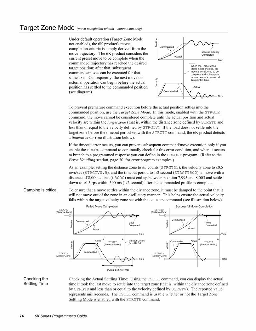
74 6K Series Programmer’s Guide
Target Zone Mode (move completion criteria—servo axes only) Under default operation (Target Zone Mode not enabled), the 6K product's move completion criteria is simply derived from the move trajectory. The 6K product considers the current preset move to be complete when the commanded trajectory has reached the desired target position; after that, subsequent commands/moves can be executed for that same axis. Consequently, the next move or external operation can begin before the actual position has settled to the commanded position (see diagram).
�������
.���
0�����
����� ���
!���
!���
����� ���
.���
/�� �����.������1� ��������� ���� ����4������(������ ��������������������� ���������� ���(���� �����5���������������� ��� ������
��(������������������
To prevent premature command execution before the actual position settles into the commanded position, use the Target Zone Mode. In this mode, enabled with the STRGTE command, the move cannot be considered complete until the actual position and actual velocity are within the target zone (that is, within the distance zone defined by STRGTD and less than or equal to the velocity defined by STRGTV). If the load does not settle into the target zone before the timeout period set with the STRGTT command, the 6K product detects a timeout error (see illustration below).
If the timeout error occurs, you can prevent subsequent command/move execution only if you enable the ERROR command to continually check for this error condition, and when it occurs to branch to a programmed response you can define in the ERRORP program. (Refer to the Error Handling section, page 30, for error program examples.)
As an example, setting the distance zone to ±5 counts (STRGTD5), the velocity zone to ≤0.5 revs/sec (STRGTV0.5), and the timeout period to 1/2 second (STRGTT500), a move with a distance of 8,000 counts (D8000) must end up between position 7,995 and 8,005 and settle down to ≤0.5 rps within 500 ms (1/2 second) after the commanded profile is complete.
Damping is critical To ensure that a move settles within the distance zone, it must be damped to the point that it will not move out of the zone in an oscillatory manner. This helps ensure the actual velocity falls within the target velocity zone set with the STRGTV command (see illustration below).
���������������������
��������� �����������
���������������������
��������
�� �����
���������
6�������(����������
.�������2���4-�����7������
���������
����
���
���
����
��(���������
����������� � ��� ���������
����
����������(����������
���������������������
��������
�� ����� ��������� ����
���������
���
���
���������������������
��������� �����������
������������
Checking the Settling Time
Checking the Actual Settling Time: Using the TSTLT command, you can display the actual time it took the last move to settle into the target zone (that is, within the distance zone defined by STRGTD and less than or equal to the velocity defined by STRGTV). The reported value represents milliseconds. The TSTLT command is usable whether or not the Target Zone Settling Mode is enabled with the STRGTE command.

Chapter 3. Basic Operation Setup 75
Programmable Inputs and Outputs (onboard and external inputs & outputs) Programmable inputs and outputs allow the controller to detect and respond to the state of switches, thumbwheels, electronic sensors, and outputs of other equipment such as drives and PLCs. The I/O that can be used as programmable inputs and outputs are:
• Onboard I/O: − Limit inputs on the “LIMITS/HOME” connectors − Trigger inputs on the “TRIGGERS/OUTPUTS” connectors (pins 9, 11, 13, 15, 17,
19, 21 & 23). A “master trigger” is available (see “MASTER TRIG” terminal on the connector on top of the 6K chassis).
− Digital outputs on the “TRIGGERS/OUTPUTS” connectors (1, 3, 5 & 7)
• Expansion I/O located on I/O bricks connected to the 6K controller’s “EXPANSION I/O” connector. Each I/O brick can hold from 1 to 4 of these I/O SIM modules in any combination (each SIM module provides 8 inputs or outputs, for a total of 32 I/O points per I/O brick):
− Digital inputs − Digital outputs − Analog inputs − Analog outputs
USING THE STATE OF I/O TO CONTROL PROGRAMMED EVENTS: Based on the binary state of the inputs and outputs (binary status can be used in assignment/comparison operations using the LIM, IN and OUT operators), the controller can make program flow decisions and assign values to binary variables for subsequent mathematical operations. These operations and the associated program flow, branching, and variable commands are listed below.
Operation based on I/O State Associated Commands See Also* I/O state assigned to a binary variable LIM, [IN], [OUT], VARB Variables (page 18)
I/O state used as a basis for comparison in conditional branching & looping statements
LIM, [IN], [OUT], IF, ELSE, NIF, REPEAT, UNTIL, WAIT, WHILE, NWHILE
Program Flow Control (page 23)
Input state used as a basis for a conditional GO
[IN], GOWHEN, LIM Synchronizing Motion (page 159)
I/O state used as a basis for a program interrupt (GOSUB) conditional statement
ONIN Program Interrupts (page 29)
Mimic PLC functionality by scanning I/O states with a compiled program
PLCP, SCANP PLC Scan Mode (page 104)
* Refer also to the respective command descriptions in the 6K Series Command Reference.
I/O UPDATE RATE: The programmable inputs and outputs are sampled at the “system update rate,” which is every 2 ms. EXPANSION I/O BRICKS: If the I/O brick is disconnected or if it loses power, the controller will perform a kill (all tasks) and set error bit 18 (see ERROR). (If you disable the “Kill on I/O Disconnect” mode with KIOENØ, the 6K will not perform the kill.) The controller will remember the brick configuration (volatile memory) in effect at the time the disconnection occurred. When you reconnect the I/O brick, the controller checks to see if anything changed (SIM by SIM) from the state when it was disconnected. If an existing SIM slot is changed (different SIM, vacant SIM slot, or jumper setting), the controller will set the SIM to factory default INEN and OUTLVL settings. If a new SIM is installed where there was none before, the new SIM is auto-configured to factory defaults.

76 6K Series Programmer’s Guide
Programmable I/O Bit Patterns The total number of onboard inputs and outputs (trigger inputs, limit inputs, digital outputs) depends on the product. The total number of expansion inputs and outputs (analog inputs, digital inputs and digital outputs) depends on your configuration of expansion I/O bricks.
These programmable I/O are represented by binary bit patterns, and it is the bit pattern that you reference when programming and checking the status of specific inputs and outputs. The bit pattern is referenced 1 to n, from left to right.
• Onboard I/O. For example, the status command to check all onboard trigger inputs is TIN. An example response for the 6K8 is: *TIN0100_0001_0000_0011_0.
• Expansion I/O. For example, the status command to check all digital inputs on I/O brick 2 is 2TIN. An example response for the 6K8 is: *2TIN0010_0110_1100_0000_XXXX_XXXX_XXXX_XXXX.
Onboard Programmable I/O
I/O Location Programming Status Report, Assignment Limit Inputs “LIMITS/HOME” connectors LIMFNC, LIMEN, LIMLVL TLIM, LIM
Trigger Inputs “TRIGGERS/OUTPUTS” connectors (pins 9, 11, 13, 15, 17, 19, 21 & 23). Master Trigger is “MASTER TRIG” on connector on top of the 6K chassis
INFNC, INLVL, INEN, ONIN, INPLC, INSTW
TIN, IN
Outputs (digital) “TRIGGERS/OUTPUTS” connectors (pins 1, 3, 5 & 7).
OUT, OUTFNC, OUTLVL, OUTEN, OUTALL, OUTPLC, OUTTW, POUT
TOUT, [OUT]
Limit Inputs (“LIMITS/HOME” connectors)
Input bit pattern for LIM, TLIM, LIMEN, LIMFNC, and LIMLVL:
Bit # Pin # Function *
1 23 Positive end-of-travel limit, axis 1. 2 21 Negative end-of-travel limit, axis 1. 3 19 Home limit, axis 1. 4 17 Positive end-of-travel limit, axis 2. 5 15 Negative end-of-travel limit, axis 2. 6 13 Home limit, axis 2. 7 11 Positive end-of-travel limit, axis 3. 8 9 Negative end-of-travel limit, axis 3. 9 7 Home limit, axis 3. 10 5 Positive end-of-travel limit, axis 4. 11 3 Negative end-of-travel limit, axis 4. 12 1 Home limit, axis 4. 13 23 Positive end-of-travel limit, axis 5. 14 21 Negative end-of-travel limit, axis 5. 15 19 Home limit, axis 5. 16 17 Positive end-of-travel limit, axis 6. 17 15 Negative end-of-travel limit, axis 6. 18 13 Home limit, axis 6. 19 11 Positive end-of-travel limit, axis 7. 20 9 Negative end-of-travel limit, axis 7. 21 7 Home limit, axis 7. 22 5 Positive end-of-travel limit, axis 8. 23 3 Negative end-of-travel limit, axis 8. 24 1 Home limit, axis 8.
* The functions listed are the factory default functions; other functions may be assigned with the LIMFNC command.
Bit 17
Bit 32 Bit 1
Bit 1
I/O Brick 2
Sample response to TLIM (limit inputs status) command: *TLIM001_001_001_001_001_001_001_001

Chapter 3. Basic Operation Setup 77
Trigger Inputs (“TRIGGERS/OUTPUTS” connectors)
Outputs (“TRIGGERS/OUTPUTS” connectors)
Input bit pattern for TIN, IN, INFNC, INLVL, INEN, INPLC, INSTW, and ONIN:
Bit # Pin # Function * 1 23 Trigger input 1 (TRIG-1A). 2 21 Trigger input 2 (TRIG-1B). 3 19 Trigger input 3 (TRIG-2A). 4 17 Trigger input 4 (TRIG-2B). 5 15 Trigger input 5 (TRIG-3A). 6 13 Trigger input 6 (TRIG-3B). 7 11 Trigger input 7 (TRIG-4A). 8 9 Trigger input 8 (TRIG-4B). 9 23 Trigger input 9 (TRIG-5A). 10 21 Trigger input 10 (TRIG-5B). 11 19 Trigger input 11 (TRIG-6A). 12 17 Trigger input 12 (TRIG-6B). 13 15 Trigger input 13 (TRIG-7A). 14 13 Trigger input 14 (TRIG-7B). 15 11 Trigger input 15 (TRIG-8A). 16 9 Trigger input 16 (TRIG-8B). 17 ---- Trigger input 17 (TRIG-M).
* If the input is assigned the “trigger interrupt” function with the INFNCi-H command, it will capture the position of thededicated “n” axis identified in the input’s name (TRIG-nA and TRIG-nB). TRIG-M captures the position of the master encoder, as well as all axes.
Output bit pattern for TOUT, [OUT], OUT, OUTFNC, OUTLVL, OUTEN, OUTALL, OUTPLC, OUTTW, POUT:
Bit # Pin # Function 1 7 Output 1. 2 5 Output 2. 3 3 Output 3. 4 1 Output 4. 5 7 Output 5. 6 5 Output 6. 7 3 Output 7. 8 1 Output 8.
“MASTER TRIG”
Sample response to TIN (trigger inputs status) command: *TIN0000_0010_1100_0000_0
Sample response to TOUT (onboard outputs status) command: *TOUT0000_0000

78 6K Series Programmer’s Guide
Expansion I/O Bricks The 6K product allows you to expand your system I/O by connecting up to 8 I/O bricks (see Installation Guide for connections). Expansion I/O bricks can be ordered separately (referred to as the “EVM32”). Each I/O brick can hold from 1 to 4 of these I/O SIM modules in any combination:
SIM Type Programming Status Report, Assignment Digital Inputs SIM (8 inputs) INFNC, INLVL, INEN, ONIN, INPLC, INSTW TIN, IN, TIO
Digital Outputs SIM (8 outputs) OUT, OUTFNC, OUTLVL, OUTEN, OUTALL, OUTPLC, OUTTW, POUT
TOUT, [OUT], TIO
Analog Inputs SIM (8 inputs) • Enable/Disable: ANIEN. • Voltage range: ANIRNG. • Joystick setup: JOYAXH, JOYAXL, JOYCDB, JOYCTR, JOYEDB, JOYZ. • Servo feedback: ANIFB, SFB • Following master source: ANIMAS, FOLMAS
• Voltage: TANI, ANI, TIO • Servo position: TPANI, PANI, FB, TFB
Analog Outputs SIM (8 outputs) ANO TANO, [ANO], TIO
Each I/O brick has a unique “brick address”, denoted with the “<B>” symbol in the command syntax. The I/O bricks are connected in series to the “EXPANSION I/O” connector on the 6K. The 1st I/O brick has address 1, the next brick has address 2, and so on. (NOTE: If you leave out the brick address in the command, the 6K product assumes you are addressing the command to the onboard I/O.) Each I/O brick has 32 I/O addresses, referenced as absolute I/O point locations:
• SIM slot 1 = I/O points 1-8 • SIM slot 2 = I/O points 9-16 • SIM slot 3 = I/O points 17-24 • SIM slot 4 = I/O points 25-32
Example
Slot #1 (I/O points 1-8)
Slot #2 (I/O points 9-16)
Slot #3 (I/O points 17-24)
Slot #4 (I/O points 25-32)
Slot #1 (I/O points 1-8) Digital Inputs SIM
I/O Brick #1 6K Controller
Slot #2 (I/O points 9-16) Digital Inputs SIM
Slot #3 (I/O points 17-24) Digital Inputs SIM
Slot #4 (I/O points 25-32) Analog Inputs SIM
Digital Outputs SIM
I/O Brick #2
Digital Inputs SIM
No SIMM installed
Digital Outputs SIM
The TIO command identifies the connected I/O bricks (and installed SIMs), including the status of each I/O point: *BRICK 1: SIM Type Status Function 1-8: DIGITAL INPUTS 0000_0000 AAAA_AAAA 9-16: DIGITAL INPUTS 0000_0000 AAAA_AAAA 17-24: DIGITAL INPUTS 0000_0000 AAAA_AAAA 25-32: ANALOG INPUTS 0.000,0.000,0.000,0.000,0.000,0.000,0.000,0.000 *BRICK 2: SIM Type Status Function 1-8: DIGITAL OUTPUTS 0000_0000 AAAA_AAAA -- SINKING 9-16: DIGITAL INPUTS 0000_0000 AAAA_AAAA 17-24: NO SIM PRESENT 25-32: DIGITAL OUTPUTS 0000_0000 AAAA_AAAA -- SOURCING
Sample response to 1TIN (digital inputs status) command: *1TIN0000_0010_1100_0000_0100_0001_XXXX_XXXX
Sample response to 2TOUT (digital outputs status) command: *2TOUT0000_0000_XXXX_XXXX_XXXX_XXXX_0000_0000

Chapter 3. Basic Operation Setup 79
Input Functions
Programmable input functions can be assigned to the onboard limit and trigger inputs, as well as to digital inputs on an expansion I/O brick connected to the 6K product. The appropriate input function command (LIMFNC or INFNC) depends on which input you are configuring:
• Onboard limit inputs (on the “LIMITS/HOME” connector) — use LIMFNC:
Axis number (optional).Some functions may be made specific to one axis. When shippedfrom the factory, all limit inputs are assigned the limit function forthe respective axis. For example, limit input 1 is assigned thepositive travel end-of-travel limit function for axis 1 (LIMFNC1-1R).
Letter that selects the desiredfunction (see list below).
Syntax: LIMFNCi-<a>c
• Onboard trigger inputs (on the “TRIGGERS/OUTPUTS” connector) and digital inputs installed on an expansion I/O brick — use INFNC:
Axis number (optional).Some functions may be madespecific to one axis. For example,to assign the 2nd input on SIMM2(I/O point #9) of I/O brick 1 to bethe stop input for axis 2 only, usethe 1INFNC9-2D command.
I/O Brick number.Trigger inputs are consideredcollectively as I/O brick 0 (zero),and are addressed of the I/O bricknumber is left off the command.
Letter that selects the desiredfunction (see list below).
<B>INFNCi-<a>cSyntax:
Virtual Inputs Virtual Inputs provide programming input functionality for data or external events that are not ordinarily represented by inputs. The Virtual Input Override (IN) command allows you to substitute almost any 32-bit data operand as a virtual input brick of 32 inputs (integer values are converted to binary). Page 8 provides a list of the data operands; the only data operands that are not allowed are: SIN, COS, TAN, ATAN, VCVT, SQRT, VAR, TW, READ, DREAD, DREADF, DAT, DPTR, and PI.
The virtual inputs behave similar to real inputs in that they are affected by INEN and INLVL, and they affect INFNC, INPLC, INSTW, INDUST, ONIN, and GOWHEN(<B>IN=b<bbbb>) commands. Unlike real inputs, virtual inputs are not affected by the INDEB debounce setting.
NOTE: A virtual input can only be defined for expansion I/O bricks that are not connected on the serial I/O network (remember that up to 8 I/O bricks are allowed). For example, if your 6K unit has two I/O bricks, you can designate I/O bricks 3-8 as virtual I/O bricks.
EXAMPLE: Suppose a PLC is sending binary data via the VARB1 command to the 6K. If the binary state of VARB1 is assigned to input brick 2 (2IN=VARB1), the 6K can respond based on programmable input functions set up with the INFNC command.
2TIN ; Brick 2 is not connected; therefore, the 6K will ; respond with an error message: "*INCORRECT I/O BRICK" 2IN=VARB1 ; Map the binary state of VARB1 to be the input state ; of "virtual" input brick 2 (2IN) VARB1=b10100000 ; Change "virtual" input brick 2IN to a new VARB1 value 2TIN ; Check the input status. The response will be: ; "*2IN1010_0000_0000_0000_0000_0000_0000_0000"
Number of the input. (see page 141 for input bit assignments)
Number of the input. (see page 143 for input bit assignments)

80 6K Series Programmer’s Guide
Letter Designator Function A..................General-purpose input (default function for triggers & inputs on I/O bricks) B..................BCD program select C..................Kill <a>D..................Stop (axis designator “a” is optional) E..................Pause/Continue F..................User fault G..................<RESERVED> H..................Trigger Interrupt for position capture or registration (trigger inputs only). Special
trigger functions can be assigned with the TRGFN command (see page 162). I..................Cause an “Alarm Event” over the Ethernet interface aJ..................Jog in the positive-counting direction (axis designator is required) aK..................Jog in the negative-counting direction (axis designator is required) aL..................Jog velocity select (axis designator is required) M..................Joystick release N..................Joystick axis select O..................Joystick velocity select P..................One-to-one program select Q..................Program security aR..................End-of-travel limit for positive-counting direction (axis designator is required) * aS..................End-of-travel limit for negative-counting direction (axis designator is required) * aT..................Home limit (axis designator is required) *
* Limit inputs (on the “LIMITS/HOME” connector) are factory-set to their respective end-of-travel or home limit function (see page 57).
NOTES • Multi-tasking: If the LIMFNC or INFNC command does not include the task identifier (%) prefix,
the function affects the task that executes the LIMFNC or INFNC command. The only functions that can be directed to a task with % are: C, D (without an axis specified), E, F, and P (e.g., 2%INFNC3-F assigns onboard input 3 as a user fault input for task 2). Multiple tasks can share the same input, but the input can only be assigned one function.
• Limit of 32 functions per input group: You can assign a maximum of 32 LIMFNC functions, and a maximum of 32 INFNC functions. For LIMFNC, this excludes functions A (“general-purpose”) and R, S, and T (end-of-travel and home limit input functions). For INFNC, this excludes functions A (“general-purpose”) and H (“trigger interrupt”).
Input Status * The purpose of the IN and LIM operators is to use the state of the inputs as a basis for conditional statements (IF, REPEAT, WHILE, GOWHEN, etc.) or for binary variable assignments (VARB). For examples, see the Conditional Looping and Branching section on page 25, and Synchronizing Motion on page 159.
Limit inputs (LIMFNC): • Status display commands:
- LIMFNC...............Active state and programmed function of all limit inputs - LIMFNCi ............Same as LIMFNC display, but only for the input number (“i”) - TLIM ...................Hardware state of all limit inputs (binary report);
use TLIM.i to check the state of only one input (“i”)
• Status assignment/comparison operator: * - LIM ......................Hardware state (binary) of all limit inputs;
use LIM.i to check the state of only one input (“i”)
Trigger inputs and digital inputs on expansion I/O bricks (INFNC): • Status display commands:
- TIO ......................I/O brick configuration (which SIMs are present) - INFNC .................Active state and programmed function of all trigger inputs - INFNCi...............Same as INFNC display, but only for the trigger input number (“i”) - <B>INFNC ..........Active state and programmed function of all inputs on I/O brick B - <B>INFNCi........Same as INFNC display, but only for the input number (“i”) on brick B - TIN ......................Hardware state of all onboard trigger inputs (binary report);
use TIN.i to check the state of only one input (“i”) - <B>TIN...............Hardware state of all digital inputs on I/O brick B (binary report) ;
use <B>TIN.i to check the state of only one input (“i”) on brick B
• Status assignment/comparison operator: * - <B>IN .................Hardware state (binary) of triggers and expansion digital inputs;
use <B>IN.i to check the state of only one input (“i”) on brick B

Chapter 3. Basic Operation Setup 81
Input Active Levels Many people refer to a voltage level when referencing the state of programmable inputs and outputs. Using LIMLVL (for limit inputs) and INLVL (for triggers and I/O brick inputs), you can define the logic levels of the programmable inputs as positive or negative. The 6K product defaults to an input level of zero volts as its active level (referred to as “active low”); thus, a “1” will appear in a status command (TLIM & LIM, or TIN & IN) referencing an input state when the voltage level is zero volts.
Active Level Setting State LIM/TLIM or IN/TIN Report Active Low, the default setting • LIMLVL0 for limits • INLVL0 for triggers/I/O bricks
Grounded — sinking current (device drive the input is on) ------------------------------------------------ Not Grounded — not sinking current (device drive the input is off)
1 (active) --------------------------------------- 0 (inactive)
Active High • LIMLVL1 for limits • INLVL1 for triggers/I/O bricks
Grounded — sinking current (device drive the input is on) ------------------------------------------------ Not Grounded — not sinking current (device drive the input is off)
0 (inactive) --------------------------------------- 1 (active)
Input Debounce Time
Using the INDEB command, you can change the input debounce time for programmable inputs. The debounce is the period of time that the input must be held in a certain state before the controller recognizes it. This directly affects the rate at which the inputs can change state and be recognized. The default setting is 4 ms. For example, to set the debounce for all digital inputs on I/O brick 2 to 5 ms, use the 2INDEB6 command.
Exception for Trigger Inputs: For trigger inputs that are assigned the “Trigger Interrupt” function (INFNCi-H), the debounce is instead governed by the TRGLOT setting. The TRGLOT setting applies to all trigger inputs defined as “Trigger Interrupt” inputs. The TRGLOT debounce time is the time required between a trigger’s initial active transition and its secondary active transition. This allows rapid recognition of a trigger, but prevents subsequent bouncing of the input from causing a false position capture. The default TRGLOT setting is 24 ms.
Limit Inputs. The limit inputs found on the “LIMITS/HOME” connectors are not normally debounced; however, if a limit is assigned a different function with the LIMFNC command (other than LIMFNCi-R, LIMFNCi-S, or LIMFNCi-T), the input is debounced using the INDEB setting for the on-board trigger inputs (I/O brick 0). If a I/O brick input or an onboard trigger input is assigned a limit input function (INFNCi-R, INFNCi-S, or INFNCi-T), the input will not be debounced.
“General Purpose” • LIMFNCi-A • INFNCi-A
This is the default function for INFNC inputs (triggers and I/O brick inputs). When an input is defined as a General Purpose input, the input is used as a standard input. You can then use this input to synchronize or trigger program events, through the use of the LIM or IN operator.
Example DEL prog1 ; Precaution: Delete a program before defining it DEF prog1 ; Begin definition of program prog1 INFNC1-A ; No function (general purpose) for trigger input 1 INFNC2-A ; No function (general purpose) for trigger input 2 INFNC3-D ; Trigger input 3 is a stop input (all axes) A10 ; Set acceleration V10 ; Set velocity D5 ; Set distance WAIT(IN=b1XX) ; Wait for onboard trigger input 1 GO1 ; Initiate motion IF(IN=bX1) ; If onboard trigger input 2 1TFB ; Transfer feedback device position for axis 1 NIF ; End IF statement END ; End definition of program prog1

82 6K Series Programmer’s Guide
BCD Program Select • LIMFNCi-B • INFNCi-B
The BCD program select function allows you to execute defined programs by activating the program select inputs.
BCD program select inputs are assigned BCD weights, with the least weight on the smallest numbered input. The next BCD weight is assigned to the next input defined as a BCD input. For example, the table to the right shows the BCD weights if inputs 1-8 are configured as program select inputs.
Input No. Input 1 Input 2 Input 3 Input 4 Input 5 Input 6 Input 7 Input 8
BCD Weight 1 2 4 8 10 20 40 80
To execute a particular program, you activate the combination of inputs to achieve the BCD weight that corresponds to the number of the program (see note below). For example, if inputs 1-8 are defined as BCD inputs (as in the example above), activating inputs 4 and 6 would execute program 28, activating inputs 1 and 4 would execute program 9, and so on.
Program Numbers A program's number is determined by the order in which the program was downloaded to the controller. The number of each program stored in the controller's memory can be obtained through the TDIR command — refer to the number reported in front of each program name. When selecting programs with BCD Program Select inputs, a program is executed when the total BCD weight of the active BCD inputs equals the program's number. When selecting programs with One-to-One Program Select inputs, the program number is assigned to one specific input and is executed when that input is activated.
Before you can execute programs using the BCD program select inputs, you must first enable scanning with the INSELP1 command. Once enabled, the controller will continuously scan the BCD inputs and execute the program (by number) according to the weight of the currently active BCD inputs. After executing and completing the selected program, the controller will scan the inputs again. NOTE: To disable scanning, enter !INSELPØ or place INSELPØ in a program that can be selected.
The INSELP command also determines how long the BCD program select input level must be maintained before the controller executes the program. This delay is referred to as debounce time (but is not affected by the INDEB setting).
Example
The number in front of each program name is
the BCD weight required to execute the program.
RESET ; Return controller to power-up conditions ERASE ; Erase all programs DEF PROG1 ; Begin definition of program PROG1 TPE ; Transfer position of encoders END ; End program DEF PROG2 ; Begin definition of program PROG2 TREV ; Transfer software revision END ; End program DEF PROG3 ; Begin definition of program PROG3 TSTAT ; Transfer statistics END ; End program INFNC1-B ; Assign onboard input 1 as a BCD program select input INFNC2-B ; Assign onboard input 2 as a BCD program select input INSELP1,50 ; Enable scanning inputs, levels must be maintained for 50ms TDIR ; Display number and name of programs stored in memory ; response from TDIR should be similar to following: ; *1 - PROG1 USES 6 BYTES ; *2 - PROG2 USES 18 BYTES ; *3 - PROG3 USES 99 BYTES ; *32877 OF 33000 BYTES (98%) PROGRAM MEMORY REMAINING ; *500 OF 500 SEGMENTS (100%) COMPILED MEMORY REMAINING
You can now execute the programs by activating the correct combination of inputs: • Activate trigger input 1 (BCD weight of 1) to execute program 1 (PROG1) • Activate trigger input 2 (BCD weight of 2) to execute program 2 (PROG2) • Activate trigger inputs 1 & 2 (BCD weight of 3) to execute program 3 (PROG3)

Chapter 3. Basic Operation Setup 83
Kill • LIMFNCi-C • INFNCi-C
When an input defined as a Kill input goes active:
• Motion stops on all axes (using the LHAD and LHADA decel rate). • Program currently in progress is terminated. • Commands currently in the command buffer are eliminated. • Drives are left in the enabled state (@DRIVE1), unless the “disable drive on kill”
function is enabled with the KDRIVE command (see description on page 48). • If error-checking bit 6 is enabled (e.g., ERROR.6-1), the error status is reported by bit
6 of the TERF, TER and ER commands and the error program (assigned with the ERRORP command) will be executed to respond to the error condition.
NOTE: Kill is not intended as a means to temporarily inhibit motion; use the Pause/Continue input function instead (LIMFNCi-E or INFNCi-E).
Stop • LIMFNCi-<a>D • INFNCi-<a>D
An input defined as a Stop input will stop motion on one or all axes (see examples below). Deceleration is controlled by the programmed AD/ADA deceleration ramp. If error-checking bit 8 is enabled (e.g., ERROR.8-1), the error status is reported by bit 8 of the TERF, TER and ER commands and the error program (assigned with the ERRORP command) will be executed to respond to the error condition.
After the Stop input is received, further program execution is dependent upon the COMEXS command setting:
COMEXSØ: (default setting) Upon receiving a stop input, motion will stop, program execution will be terminated and cannot be resumed, and every command in the buffer will be discarded (exception: an axis-specific stop input does not dump the command buffer).
COMEXS1: Upon receiving a stop input, motion will stop, program execution will pause, and all commands following the command currently being executed will remain in the command buffer (but the move in progress will not be saved).
You can resume program execution (but not the move in progress) by issuing an immediate Continue (!C) command or by activating a pause/continue input (i.e., a general-purpose input configured as a pause/continue input with the INFNCi-E command—see below). You cannot resume program execution while the move in progress is decelerating.
COMEXS2: Upon receiving a stop input, the 6K responds as it does in the COMEXS0 mode, with the exception that you can still use the program-select inputs to select programs (INSELP value is retained). The program-select input functions are: BCD select (INFNCi-B or LIMFNCi-B; see page 82), and one-to-one select (INFNCi-P or LIMFNCi-P; see page 88). For further details on program selection with inputs, see INFNC (or LIMFNC) and INSELP.
Example 1 (stop all axes): The 3INFNC2-D command assigns the “stop” function to the 2nd input on SIM1 of I/O brick 3. When this input is activated, all axes will stop.
Example 2 (stop a specific axis): The 3INFNC2-4D command assigns the “stop” function to the 2nd input on SIM1 of I/O brick 3, but makes it specific only to the motion on axis 4. When this input is activated, only the motion on axis 4 axes will stop.
Pause/Continue • LIMFNCi-E • INFNCi-E
An input defined as a Pause/Continue input will affect motion and program execution depending on the COMEXR command setting, as described below. In both cases, when the input is activated, the current command being processed will be allowed to finish executing before the program is paused.
COMEXRØ: Upon receiving a pause input, only program execution will be paused; any motion in progress will continue to its predetermined destination. Releasing the pause

84 6K Series Programmer’s Guide
input or issuing a !C command will resume program execution.
COMEXR1: Upon receiving a pause input, both motion and program execution will be paused; the motion stop function is used to halt motion. Releasing the pause input or issuing a !C command will resume motion and program execution. You cannot resume program execution while the move in progress is decelerating.
User Fault • LIMFNCi-F • INFNCi-F
An input defined as a User Fault input acts as an immediate Kill (!K) command, stopping motion on all axes and terminating program execution. Motion is stopped at the rate set with the hard limit (LHAD & LHADA) commands.
If error-checking bit 7 is enabled (e.g., ERROR.7-1), then a user fault input will cause a branch to the ERRORP error program (for more information, see Error Handling on page 30) and the occurrence of a user fault input will be reported by error bit 7 (see TERF, TER and ER commands).
Trigger Interrupt (INFNCi-H)
This function is available only for onboard trigger inputs. Any trigger input can be defined as a Trigger Interrupt input and can be used for these functions:
• Position Capture (see below) • Special trigger functions assigned with the TRGFN command (see below) • Registration (see discussion on page 155)
Notes About Trigger Interrupt Inputs
• The trigger interrupt input is debounced for 24 ms (default) before another input on the same trigger is recognized. If your application requires a different debounce time, you can change it with the TRGLOT command (see Input Debounce Time on page 81).
• When configured as Trigger Interrupts, the triggers cannot be affected by the input enable (INEN) command.
• Status: Use the TTRIG and TRIG commands to ascertain if a trigger interrupt input has been activated. TTRIG displays the status as a binary report, and TRIG is an assignment/comparison operator for using the status information in a conditional expression (e.g., in an IF statement). Each TTRIG/TRIG bit is cleared when the respective captured position value is read with the PCC, PCE, PCME, PCMS, TPCC, TPCE, TPCME, or TPCMS commands, but the position information is still available from the respective register until it is overwritten by a subsequent position capture by the same trigger input.
Position Capture Each axis has two dedicated trigger inputs, referred to as “TRIG-nA” and “TRIG-nB” (n = number of the axis). These trigger inputs are located on the 25-pin “TRIGGERS/OUTPUTS” connector. When either trigger input (TRIG-nA or TRG-nB) for a particular axis is assigned the Trigger Interrupt function, activating the input performs a hardware capture of that axis’ position. If the axis is used as a follower in Following, activating the trigger also performs an interpolated capture of the associated master axis position.
An additional trigger, labeled “TRIG-M”, can be used to perform a hardware capture of the Master Encoder (the encoder connected to the “MASTER ENCODER” connector), as well as the position of all axes (encoder position on servo axes; commanded or encoder position for steppers, depending on the ENCCNT setting). To assign TRIG-M as a trigger interrupt input, use the INFNC17-H command.
When a Trigger Interrupt input is activated, the controller captures the relevant positions and stores them in registers that are available at the next system update (2 ms) through the use of these transfer and assignment/comparison commands:

Chapter 3. Basic Operation Setup 85
Captured Information Transfer Assignment/Comparison Offset * Scale Factor ** Commanded position TPCC PCC PSET SCLD Encoder position TPCE PCE PSET SCLD Master encoder position TPCME PCME PMESET SCLMAS Master cycle position TPCMS PCMS PSET SCLMAS
* Captured values are offset by any existing PSET or PMESET offset. ** If scaling is enabled, the captured position is scaled by SCLD or SCLMAS.
Notes About Position Capture • Hardware Capture: The encoder position is captured within ± 1 encoder count. The
commanded position capture accuracy is ± 1 count.
• Interpolated Capture: There is a time delay of up to 50 µs between activating the trigger interrupt input and capturing the position; therefore, the accuracy of the captured position is equal to 50 µs multiplied by the velocity of the axis at the time the input was activated.
• Servo vs. Stepper. The nature of the axis position captured with a Trigger Interrupt input can be different, depending on whether the axis is configured for servo or stepper operation (AXSDEF command setting). For servo axes, both the commanded and encoder position for the axis are captured. Analog input feedback cannot be captured. For stepper axes, if the ENCCNT command is set to ENCCNT0 (default condition), only the commanded position is captured. If ENCCNT1 mode is enabled, only the encoder position is captured.
Trigger Functions The Trigger Functions command (TRGFN) allows you to assign additional functions to trigger inputs that have been defined as trigger interrupt inputs with the INFNCi-H command. These trigger functions are cleared once the function is triggered. Command syntax is:
!��������� �"#����������$�������
������
����%�&�'�����!�� ����������$�������
������ ������������(����������������))�����*�����+'����������+�� �����'������� ���,�������
�(������,�
• “Conditional GO” Function (aTRGFNc1x): Suspend execution of the next start-motion command until the specified trigger input goes active. Start-motion commands are:
- GO (standard command to begin motion) - GOL (begin linear interpolated motion) - FSHFC (begin continuous shift – for Following motion) - FSHFD (begin preset shift – for Following motion)
Axis status bit 26 (reported with TASF, TAS, or AS) is set to one (1) when there is a pending “Conditional GO” condition initiated by a TRGFN command; this bit is cleared when the trigger is activated or when a stop command or a kill command is issued. If you need execution to be triggered by other factors (e.g., input state, master position, encoder position, etc.) use the GOWHEN command; see GOWHEN command or page 159 for details.
• “New Master Cycle” Function (aTRGFNcx1): This is equivalent to executing the FMCNEW command. When the specified trigger input goes active, the controller begins a new Following master cycle. Refer to the FMCNEW command or to page 184 for more on master cycles.
Code Examples INFNC2-H ; Assign trigger 1B (onboard input 2) to ; function as a trigger interrupt input. 1TRGFNBx1 ; When trigger 1B goes active, axis 1 will begin ; a new master cycle 2TRGFNB1 ; When trigger 2B goes active, axis 2 will execute ; the move commanded with the GO command. GO01 ; The move on axis 2 is commanded, but will not

86 6K Series Programmer’s Guide
; execute until trigger 2B becomes active.
Registration If registration is enabled (with the RE command), activating a trigger interrupt input will initiate registration move(s) defined with the REG command. Refer to page 155 for details on the Registration feature.
Alarm Event • LIMFNCi-I • INFNCi-I
An input specified as an Alarm Even input will cause the 6K controller to set an Alarm Event in the Communications Server over the Ethernet interface. You must first enable the Alarm checking bit for this input-driven alarm (INTHW.23-1). For details on Communications Server features, see the Com6srvr User’s Guide for Gemini & 6K Series Products.
Jogging the Motor • LIMFNCi-aJ • LIMFNCi-aK • LIMFNCi-aL • INFNCi-aJ • INFNCi-aK • INFNCi-aL
In some applications, you might want to manually move (jog) the load. You can configure these jog-related input functions:
“J” ....Jog in the positive counting direction when the input is active, stop when the input is inactive.
“K” ....Jog in the negative counting direction when the input is active, stop when the input is inactive.
“L” ....Select the high (JOGVH) or low (JOGVL) velocity setting for jog motion. Activating the input selects high velocity, deactivating the input selects low velocity.
The jog profile is defined with these commands listed below. NOTE: If scaling is enabled (SCALE1) the velocity is scaled by SCLV and accel/decel is scaled by SCLA.
JOGVH .......High velocity range for jogging. The high velocity is used when the jogging speed-select input (configured with INFNCi-aL) is active.
JOGVL .......Low velocity range for jogging. The low velocity is used when the jogging speed-select input (configured with INFNCi-aL) is inactive.
JOGA ..........Jog acceleration JOGAA .......Jog acceleration (s-curve profile) JOGAD .......Jog deceleration JOGADA .....Jog deceleration (s-curve profile)
Once you set up the jog functions and move profile, you can attach a switch to the designated jog inputs and perform jogging. (Jog motion will not occur unless Jog Mode is enabled with the JOG command.) The example below shows you how to define a program to set up jogging.
Example Step 1 Define program for jog setup: DEF prog1 ; Begin definition of program prog1 JOGA25 ; Jog acceleration to 25 units/sec/sec JOGAD25 ; Jog deceleration to 25 units/sec/sec JOGVL.5 ; Low-speed jog velocity to 0.5 units/sec JOGVH5 ; High-speed jog velocity to 5 units/sec INFNC1-1J ; Trigger input 1 is a positive-direction jog input, axis 1 INFNC2-1K ; Trigger input 2 is a negative-direction jog input, axis 1 INFNC3-1L ; Trigger input 3 is a speed-select input, axis 1 JOG1 ; Enable Jog function for axis 1 END ; End program definition
Step 2 Download and run the prog1 program.
Step 3 Activate trigger input 1 to move the load on axis 1 in the positive direction at a velocity of 0.5 units/sec (until trigger input 1 is released). Deactivate the input to stop the axis.

Chapter 3. Basic Operation Setup 87
Step 4 Activate trigger input 2 to move the load on axis 1 in the negative direction at a velocity of 0.5 units/sec (until trigger input 2 is released). Deactivate the input to stop the axis.
Step 5 Activate trigger input 3 to switch to high-speed jogging.
Step 6 Repeat steps 3 and 4 to perform high-speed jogging at the JOGVH value (5 rps).
Joystick Functions • LIMFNCi-M • LIMFNCi-N • LIMFNCi-O • INFNCi-M • INFNCi-N • INFNCi-O
As part of the joystick setup process, you can configure programmable inputs to serve the joystick input functions listed below. Full details on joystick setup and operation are provided on page 114.
“M” ....The Joystick Release input signals the controller to end joystick operation and resume program execution with the next statement in your program. When the input is open (high, sinking current), the joystick mode is disabled (joystick mode can be enabled only if the input is closed, and only with the JOY command). When the input is closed (low, not sinking current), joystick mode can be enabled with the JOY command. The general process of using Joystick mode is: 1. Assign the “Joystick Release” input function to a programmable input. 2. At the appropriate place in the program, enable joystick control of motion (with the JOY
command). (Joystick mode cannot be enabled unless the "Joystick Release" input is closed.) When the JOY command enables joystick mode for the affect axes, program execution stops on those axes (assuming the Continuous Command Execution Mode is disabled with the COMEXCØ command).
3. Use the joystick to move the axes as required. 4. When you are finished using the joystick, open the “Joystick Release” input to disable the
joystick mode. This allows program execution to resume with the next statement after the initial JOY command that started the joystick mode.
“N” ....The Joystick Axis Select input allows you to control two pairs of axes with one joystick. Use the JOYAXH and JOYAXL commands to assign analog inputs to control specific axes. Opening the Axis Select input (input is high, sinking current) selects the JOYAXH configuration. Closing the Axis Select input (input is low, not sinking current) selects the JOYAXL configuration.
“O” ....The Joystick Velocity Select input allows you to select the velocity for joystick motion. The JOYVH and JOYVL commands establish the high-speed velocity and the low-speed velocity, respectively. Opening the Velocity Select input (input is high, sinking current) selects the JOYVH configuration. Closing the Velocity Select input (input is low, not sinking current) selects the JOYVL configuration. The high range could be used to quickly move to a location, the low range could be used for accurate positioning. NOTE: When this input is not connected, joystick motion always uses the JOYVL velocity setting.
88 6K Series Programmer’s Guide
One-to-One Program Select • LIMFNCi-iP • INFNCi-iP
An input defined as a One-to-One Program Select input is assigned to execute one specific program. The targeted program is reference by its number (see note).
Program Numbers A program’s number is determined by the order in which the program was downloaded to the controller. The number of each program stored in the controller's memory can be obtained through the TDIR command — refer to the number reported in front of each program name. When selecting programs with One-to-One Program Select inputs, the program number is assigned to one specific input and is executed when the input is activated (see example below).
Before you can execute programs using the One-to-One program select inputs, you must first enable scanning with the INSELP2 command. Once enabled, the controller will continuously scan the inputs and execute the program (by number) according to the program number assigned to the input. After executing and completing the selected program, the controller will scan the inputs again. NOTE: To disable scanning, enter !INSELPØ or place INSELPØ in a program that can be selected.
The INSELP command also determines how long the program select input level must be maintained before the controller executes the program. This delay is referred to as debounce time (but is not affected by the INDEB setting).
Example RESET ; Return controller to power-up default conditions DEF proga ; Begin definition of program proga TFB ; Transfer position of feedback devices END ; End program DEF progb ; Begin definition of program progb TREV ; Transfer software revision END ; End program DEF progc ; Begin definition of program progc TSTAT ; Transfer statistics END ; End program TDIR ; Response should show: *1 - PROGA USES 36 BYTES
; *2 - PROGB USES 70 BYTES ; *3 - PROGC USES 133 BYTES
INFNC4-1P ; Trigger input 4 (TRIG-2B) will select proga INFNC5-2P ; Trigger input 5 (TRIG-3A) will select progb INFNC6-3P ; Trigger input 6 (TRIG-3B) will select progc INSELP2,50 ; Enable scanning of inputs with a strobe time of 50 ms
You can now execute programs by making a contact closure from an input to ground to activate the input:
• Activate trigger input 4 to execute program 1 (proga) • Activate trigger input 5 to execute program 2 (progb) • Activate trigger input 6 to execute program 3 (progc)

Chapter 3. Basic Operation Setup 89
Program Security • LIMFNCi-Q • INFNCi-Q
Once an input is assigned the Program Security function, the Program Security feature is enabled. The program security feature denies you access to the DEF, DEL, ERASE, MEMORY, LIMFNC and INFNC commands until you activate the Program Security input. Being denied access to these commands effectively restricts altering the user memory allocation. If you try to use these commands when program security is active (program security input is not activated), you will receive the error message *ACCESS DENIED.
For example, once you issue the 2INFNC7-Q command, input 7 on I/O brick 2 (2IN.7) is assigned the program security function and access to the DEF, DEL, ERASE, MEMORY, LIMFNC and INFNC commands will be denied until you activate 2IN.7.
To regain access to the DEF, DEL, ERASE, MEMORY, LIMFNC or INFNC commands without the use of the program security input, you must issue the INEN command to disable the program security input, make the required user memory changes, and then issue the INEN command to re-enable the input. For example, if input 3 on brick 2 is assigned as the Program Security input, use 2INEN.3=1 to disable the input and leave it activated, make the necessary user memory changes, and then use 2INEN.3=E to re-enable the input.
NOTE: If you wish the Program Security feature to be enabled on power-up, place the INFNCi-Q or LIMFNCi-Q command in the start-up program (STARTP).
Limit Functions • LIMFNCi-aR • LIMFNCi-aS • LIMFNCi-aT • INFNCi-aR • INFNCi-aS • INFNCi-aT
The inputs on the “LIMITS/HOME” connectors are factory-configured with the LIMFNC command to function as end-of-travel and home limits for the respective axes (see illustration on page 76). The limit functions are:
“R” .... Positive-Direction End-of-Travel Limit input, axis specific. “S” .... Negative-Direction End-of-Travel Limit input, axis specific. “T” .... Home Limit input, axis specific.
If you intend to use digital inputs on an external I/O brick as limit inputs: 1. Assign the limit function to the external input with the INFNC command. For example,
1INFNC9-1R assigns the “axis 1 positive end-of-travel limit” function to the 1st input on SIM2 (I/O point 9) of I/O brick 1.
2. Reassign the respective “LIMITS” input to a non-limit function with the LIMFNC command. For example, LIMFNC1-A assigns the “general-purpose input” function to limit input 1 (normally assigned the “axis 1 positive end-of-travel limit” function).
NOTE: Once a trigger or I/O brick input is assigned a limit function, it is no longer debounced (INDEB has no effect), and it must be enabled/disabled with the LH command instead of the INEN command.
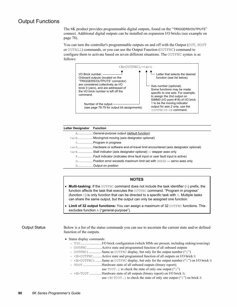
90 6K Series Programmer’s Guide
Output Functions
The 6K product provides programmable digital outputs, found on the “TRIGGERS/OUTPUTS” connect. Additional digital outputs can be installed on expansion I/O bricks (see example on page 78).
You can turn the controller's programmable outputs on and off with the Output (OUT, POUT or OUTALL) commands, or you can use the Output Function (OUTFNC) command to configure them to activate based on seven different situations. The OUTFNC syntax is as follows:
Axis number (optional). Some functions may be made specific to one axis. For example, to assign the 2nd output on SIMM3 (I/O point #18) of I/O brick 1 to be the moving indicator output for axis 2 only, use the 1OUTFNC18-2B command.
Number of the output. (see page 78-79 for output bit assignments)
I/O Brick number. Onboard outputs (located on the “TRIGGERS/OUTPUTS” connector) are considered collectively as I/O brick 0 (zero), and are addressed of the I/O brick number is left off the command.
Letter that selects the desired function (see list below).
<B>OUTFNCi-<a>c
Letter Designator Function A..................General-purpose output (default function) <a>B..................Moving/not moving (axis designator optional) C..................Program in progress <a>D..................Hardware or software end-of-travel limit encountered (axis designator optional) <a>E..................Stall indicator (axis designator optional) — stepper axes only F..................Fault indicator (indicates drive fault input or user fault input is active) G..................Position error exceeds maximum limit set with SMPER — servo axes only H..................Output on position
NOTES • Multi-tasking: If the OUTFNC command does not include the task identifier (%) prefix, the
function affects the task that executes the OUTFNC command. “Program in progress” (function C) is only function that can be directed to a specific task with %. Multiple tasks can share the same output, but the output can only be assigned one function.
• Limit of 32 output functions: You can assign a maximum of 32 OUTFNC functions. This excludes function A (“general-purpose”).
Output Status
Below is a list of the status commands you can use to ascertain the current state and/or defined function of the outputs.
• Status display commands: - TIO........................I/O brick configuration (which SIMs are present, including sinking/sourcing) - OUTFNC.................Active state and programmed function of all onboard outputs - OUTFNCi ..............Same as OUTFNC display, but only for the output number (“i”) - <B>OUTFNC..........Active state and programmed function of all outputs on I/O brick B - <B>OUTFNCi .......Same as OUTFNC display, but only for the output number (“i”) on I/O brick B - TOUT .....................Hardware state of all onboard outputs (binary report);
use TOUT.i to check the state of only one output (“i”) - <B>TOUT ..............Hardware state of all outputs (binary report) on I/O brick B;
use <B>TOUT.i to check the state of only one output (“i”) on brick B

Chapter 3. Basic Operation Setup 91
• Status assignment/comparison operator: * - OUT ........................Hardware state (binary) of all onboard outputs;
use OUT.i to check the state of only one output (“i”) - <B>OUT .................Hardware state (binary) of all outputs on I/O brick B;
use <B>OUT.i to check the state of only one output (“i”) on I/O brick B * The purpose of the OUT operator is to use the state of the outputs as a basis for conditional statements (IF, REPEAT, WHILE, GOWHEN, etc.) or for binary variable assignments (VARB).
Output Active Levels
Using OUTLVL, you can define the logic levels of the programmable outputs as positive or negative. OUTLVL0 selects active low (default setting); OUTLVL1 selects active high.
Onboard Outputs (on the “TRIGGERS/OUTPUTS” connector):
OUTLVL Setting
OUT State *
Factory Default (use internal 24V)
Use an external supply at VINref
OUT/TOUT status
OUTLVL0 (default) OUT1 Sinking current Sinking current 1 OUTLVL0 (default) OUT0 Sourcing 24V @ 0.7mA Sourcing VINref 0 OUTLVL1 OUT1 Sourcing 24V @ 0.7mA Sourcing VINref 1 OUTLVL1 OUT0 Sinking current Sinking current 0
* The output is “active” when it is commanded by the OUT, OUTP, or POUT command (for example, OUTxx1 activates output 3).
Outputs on Expansion I/O Bricks:
• Sinking vs. Sourcing Outputs. On power up, the 6K controller auto-detects the type of output SIM installed on each external I/O brick, and automatically changes the OUTLVL setting accordingly. If sinking (NPN) outputs are detected, OUTLVL is set to active low (OUTLVL0); if sourcing (PNP) outputs are detected, OUTLVL is set to active high (OUTLVL1).
• Disconnect I/O Brick. If the I/O brick is disconnected (or if it loses power), the controller will perform a kill (all tasks) and set error bit 18. (If you disable the “Kill on I/O Disconnect” mode with KIOENØ, the 6K will not perform the kill.) The controller will remember the brick configuration (volatile memory) in effect at the time the disconnection occurred. When you reconnect the I/O brick, the controller checks to see if anything changed (SIM by SIM) from the state when it was disconnected. If an existing SIM slot is changed (different SIM, vacant SIM slot, or jumper setting), the controller will set the SIM to factory default INEN and OUTLVL settings. If a new SIM is installed where there was none before, the new SIM is auto-configured to factory defaults.
• Relationships: Output Type OUTLVL Setting OUT State * Current OUT/TOUT status LED NPN (sinking) OUTLVL0 (default) OUT1 Sinking current 1 ON NPN OUTLVL0 (default) OUT0 No current flow 0 OFF NPN OUTLVL1 OUT1 No current flow 1 OFF NPN OUTLVL1 OUT0 Sinking current 0 ON PNP (sourcing) OUTLVL0 OUT1 No current flow 1 OFF PNP OUTLVL0 OUT0 Sourcing current 0 ON PNP OUTLVL1 (default) OUT1 Sourcing current 1 ON PNP OUTLVL1 (default) OUT0 No current flow 0 OFF
* The output is “active” when it is commanded by the OUT, OUTP, or POUT command (for example, OUTxx1 activates output 3).
“General Purpose” (OUTFNCi-A)
The default function for the outputs is General Purpose. As such, the output is used as a standard output, turning it on or off with the OUT, OUTP or OUTALL commands to affect processes external to the controller. To view the state of the outputs, use the TOUT command. To use the state of the outputs as a basis for conditional branching or looping statements (IF, REPEAT, WHILE, etc.), use the [ OUT ] command.

92 6K Series Programmer’s Guide
Moving/Not Moving (In Position) (OUTFNCi-<a>B)
When assigned the Moving/Not Moving function, the output will activate when the axis is commanded to move. As soon as the move is completed, the output will change to the opposite state.
Servo Axes: If the target zone mode is enabled (STRGTE1), the output will not change state until the move completion criteria set with the STRGTD and STRGTV commands has been met. (For more information, see the Target Zone section on page 74.) In this manner, the Moving/Not Moving output functions as an In Position output.
Example The code example below defines onboard outputs 1 and 2 as General Purpose outputs and output 3 as a Moving/Not Moving output. Before the motor moves 4,000 steps, output 1 turns on and output 2 turns off. These outputs remain in this state until the move is completed, then output 1 turns off and output 2 turns on. While the motor/load is moving, output 3 remains on. SCALE0 ; Disable scaling MC0 ; Set axis 1 to preset positioning mode MA0 ; Select incremental positioning mode A10 ; Set axis 1 acceleration to 10 V5 ; Set axis 1 velocity to 5 D4000 ; Set axis 1 distance to 4,000 counts OUTFNC1-A ; Set onboard output 1 as a general purpose output OUTFNC2-A ; Set onboard output 2 as a general purpose output OUTFNC3-1B ; Set onboard output 3 as axis 1 Moving/Not Moving output OUT10 ; Turn onboard output 1 on and output 2 off GO1 ; Initiates axis 1 move OUT01 ; Turn onboard output 1 off and output 2 on
Program in Progress (OUTFNCi-C)
When assigned the Program in Progress function, the output will activate when a program is being executed. After the program is finished, the output's state is reversed. The action of executing a program is also reported with system status bit 3 (see TSSF, TSS and SS commands).
Limit Encountered (OUTFNCi-<a>D)
When assigned the Limit Encountered function, the output will activate when a hard or soft end-of-travel limit has been encountered.
If a hard or soft limit is encountered, you will not be able to move the motor/load in that same direction until you clear the limit by changing direction (D) and issuing a GO command. (An alternative is to disable the limits with the LHØ command, but this is recommended only if the motor is not coupled to the load.) The event of encountering an end-of-travel limit is also reported with axis status bits 15-18 (see TASF, TAS and AS commands, summary on page 226).
Stall Indicator (OUTFNCi-<a>E) Stepper Axis Only
When assigned the Stall Indicator function, the output will activate when a stall is detected. To detect a stall, you must first connect an encoder and enable stall detection with the ESTALL1 command. Refer to Encoder-Based Stepper Operation on page 64 for further discussion on stall detection.
Fault Output (OUTFNCi-F)
When assigned the Fault Output function, the output will activate when either the user fault input or the drive fault input becomes active. The user fault input is a general-purpose input defined as a user fault input with the LIMFNCi-F or INFNCi-F command (see page 83).
Make sure the drive fault input is enabled (DRFEN) and the drive fault active level (DRFLVL) is appropriate for the drive you are using.
Maximum Position Error Exceeded (OUTFNCi-<a>G) Servo Axes Only
When assigned the Maximum Position Error Exceeded function, the output will activate when the maximum allowable position error, as defined with the SMPER command, is exceeded.
The position error (TPER) is defined as the difference between the commanded position (TPC) and the actual position as measured by the feedback device (TFB). When the maximum position error is exceeded (usually due to lagging load, instability, or loss of position feedback), the controller shuts down the drive and sets error status bit 12 (reported by the TERF, TER and ER commands if bit 12 of the ERROR command is enabled).
NOTE If the SMPER command is set to zero (SMPERØ — the default value), the position error is not monitored; thus, the Maximum Position Error Exceeded function will not be usable.

Chapter 3. Basic Operation Setup 93
Output on Position (OUTFNCi-H)
The Output on Position feature activates the designated output when the axis has reached a specified position. To use this feature, you must first assign the Output on Position function to the respective output, and define the Output on Position characteristics with the OUTP command. The OUTP command correlates directly to a specific onboard programmable output and axis (e.g., OUTPA correlates to output 1 and axis 1, OUTPB correlates to output 2 and axis 2, and so on):
OUTP n <b>, <b>, <r>, <i>
Axis/Output Specifier:
A ... Turn on output 1 based on axis #1's positionB ... Turn on output 2 based on axis #2's positionC ... Turn on output 3 based on axis #3's positionD ... Turn on output 4 based on axis #4's positionE ... Turn on output 5 based on axis #5's positionF ... Turn on output 6 based on axis #6's positionG ... Turn on output 7 based on axis #7's positionH ... Turn on output 8 based on axis #8's position
Enable Bit:
1 ... Enable the output-on-position function0 ... Disable the output-on-position function
Servo Axes: If an SFB command is executed, the function is disabled.
Increment or Absolute Position Comparison:
1 ... Set position comparison to incremental(measured from the last start-motioncommand, such as GO, GOL, GOWHEN, etc.)
0 ... Set position comparison to absolute
Position:
Scalable distance (distance is eitherincremental or absolute, depending on thesecond <b> data field).
Servo Axes:Only the encoder position can be used.
Stepper Axes: · If ENCCNT0, the commanded position is used.· If ENCCNT1, the encoder position is used.
Time (milliseconds):
Time (milliseconds) the output is to stay active.The output activates when the specifiedposition (<r>) is reached or exceeded, and stays active for the specified time.
If this field is set to zero, theoutput will stay active for as long as the actualdistance equals or exceeds the positioncomparison distance (this is possible only foran absolute position comparison).
Sample Code for Setup
In this example, the user has a two-axis application and wants to turn on output when axis 1 (servo) reaches encoder position 50,000 and turn on another output when axis 2 (stepper) reaches commanded position 30,000. Both outputs must remain on for 50 milliseconds. AXSDEF10 ; Define axis 1 as servo, axis 2 as stepper SFB1 ; Select encoder feedback for axis 1 OUTFNC1-H ; Define onboard output 1 as an "output on ; position" output OUTFNC2-H ; Define onboard output 2 as an "output on ; position" output OUTPA1,0,+50000,50 ; Turn on onboard output 1 for 50 ms when the ; encoder position of axis 1 is > or = ; absolute position +50,000 OUTPB1,1,+30000,50 ; Turn on onboard output 2 for 50 ms when the ; axis 2's commanded position reaches > or = ; incremental position 30,000 (since the last GO)
Notes about Output On Position • On servo axes, this feature can be used only with encoder feedback and is not operational
with ANI (analog input) feedback. On stepper axes, this feature can be based on commanded position or encoder position, depending on the ENCCNT setting for the particular axis (default is ENCCNT0, which uses the commanded position).
• The output activates only during motion; thus, issuing a PSET command to set the absolute position counter to activate the output on position will not turn on the output until the next motion occurs.

94 6K Series Programmer’s Guide
Variable Arrays (teaching variable data)
More on variables: see page 18.
Variable data arrays provide a method of storing (teaching) variable data and later using the stored data as a source for motion program parameters. The variable data can be any value that can be stored in a numeric (VAR or VARI) variable (e.g., position, acceleration, velocity, etc.). The variable data is stored into a data program, which is an array of data elements that have a specific address from which to write and read the variable data. Data programs do not contain 6K Series commands.
The information below describes the principles of using the data program in a teach-type application. Following that is an application example in which the joystick is used to teach position data to be used in a motion program.
Basics of Teach-Data Applications The basic process of using a data program for data teaching applications is as follows:
1. Initialize a data program. 2. Teach (store/write) variable data into the data program. 3. Read the data elements from the data program into a motion program.
1. Initialize a Data Program
This is accomplished with the DATSIZ command. The DATSIZ command syntax is DATSIZi<,i>. The first integer (i) represents the number of the data program (1 - 50). You can create up to 50 separate data programs. The data program is automatically given a specific program name (DATPi). The second integer represents the total number of data elements (up to 6,500) you want in the data program. Upon issuing the DATSIZ command, the data program is created with all the data elements initialized with a value of zero.
The data program has a tabular structure, where the data elements are stored 4 to a line. Each line of data elements is called a data statement. Each element is numbered in sequential order from left to right (1 - 4) and top to bottom (1 - 4, 5 - 8, 9 - 12, etc.). You can use the TPROG DATPi command (“i” represents the number of the data program) to display all the data elements of the data program.
For example, if you issue the DATSIZ1,13 command, data program 1 (called DATP1) is created with 13 data elements initialized to zero. The response to the TPROG DATP1 command is depicted below. Each line (data statement) begins with DATA=, and each data element is separated with a comma.
*DATA=+Ø.Ø,+Ø.Ø,+Ø.Ø,+Ø.Ø *DATA=+Ø.Ø,+Ø.Ø,+Ø.Ø,+Ø.Ø *DATA=+Ø.Ø,+Ø.Ø,+Ø.Ø,+Ø.Ø *DATA=+Ø.Ø
Each data statement, comprising four data elements, uses 43 bytes of memory. The memory for each data statement is subtracted from the memory allocated for user programs (see MEMORY command).

Chapter 3. Basic Operation Setup 95
2. Teach the Data to the Data Program
The data that you wish to write to the data elements in the data program must first be placed into numeric variables (VAR). Once the data is stored into numeric variables, the data elements in the data program can be edited by using the Data Pointer (DATPTR) command to move the data pointer to that element, and then using the Data Teach (DATTCH) command to write the datum from the numeric variable into the element.
When the DATSIZ command is issued, the internal data pointer is automatically positioned to data element 1. Using the default settings for the DATPTR command, the numberic variable data is written to the data elements in sequential order, incrementing one by one. When the last data element in the data program is written, the data pointer is automatically set to data element 1 and a warning message (*WARNING: POINTER HAS WRAPPED AROUND TO DATA POINT 1) is displayed. The warning message does not interrupt program execution.
The DATPTR command syntax is DATPTRi,i,i. The first integer (i) represents the data program number (1 through 50). The second integer represents the number of the data element to point to (1 through 6500). The third integer represents the number of data elements by which the pointer will increment after writing each data element from the DATTCH command, or after recalling a data element with the DAT command.
The DATTCH command syntax is DATTCHi<,i,i,i>. Each integer (i) represents the number of a numeric variable. The value of the numeric variable will be stored into the data element(s) of the currently active data program (i.e., the program last specified with the last DATSIZ or DATPTR command). As indicated by the number of integers in the syntax, the maximum number of variable values that can be stored in the data program per DATTCH command is 4. Each successive value from the DATTCH command is stored to the data program according to the pattern established by the third integer of the DATPTR command.
As an example, suppose data program 1 is configured to hold 13 data elements (DATSIZ1,13), the data pointer is configured to start at data element 1 and increment 1 data element after every value stored from the DATTCH command (DATPTR1,1,1), and the values of numeric variables 1 through 3 are already assigned (VAR1=2, VAR2=4, VAR3=8). If you then enter the DATTCH1,2,3 command, the values of VAR1 through VAR3 will be assigned respectively to the first three data elements in the data program, leaving the pointer pointing to data element 4. The response to the TPROG DATP1 command would be as follows (the text is highlighted to illustrate the final location of the data pointer after the DATTCH1,2,3 command is executed):
*DATA=+2.Ø,+4.Ø,+8.Ø,+Ø.Ø *DATA=+Ø.Ø,+Ø.Ø,+Ø.Ø,+Ø.Ø *DATA=+Ø.Ø,+Ø.Ø,+Ø.Ø,+Ø.Ø *DATA=+Ø.Ø
If you had set the DATPTR command to increment 2 data elements after every value from the DATTCH command (DATPTR1,1,2), the data program would be filled differently and the data pointer would end up pointing to data element 7:
*DATA=+2.Ø,+Ø.Ø,+4.Ø,+Ø.Ø *DATA=+8.Ø,+Ø.Ø,+Ø.Ø,+Ø.Ø *DATA=+Ø.Ø,+Ø.Ø,+Ø.Ø,+Ø.Ø *DATA=+Ø.Ø
3. Recall the Data from the Data Program
After storing (teaching) your variables to the data program, you can use the DATPTR command to point to the data elements and the DATi (“i” = data program number) data assignment command to read the stored variables to your motion program. You cannot recall more than one data element at a time; therefore, if you want to recall the data in a one-by-one sequence, the third integer of the DATPTR command must be a 1 (this is the default setting).

96 6K Series Programmer’s Guide
Summary of Related 6K Series Commands DATSIZ ..... Establishes the number of data elements a specific data program is to contain. A
new DATPi program name is automatically generated according to the number of the data program (i = 1 through 50). The memory required for the data program is subtracted from the memory allocated for user programs (see MEMORY command).
DATPTR ..... Moves the data pointer to a specific data element in any data program. This command also establishes the number of data elements by which the pointer increments after writing each data element from the DATTCH command and after recalling each data element with the DAT command.
DATTCH ..... Stores the variable data into the data program specified with the last DATSIZ or DATPTR command. After the data is stored, the data pointer is incremented the number of times entered in the third integer of the DATPTR command. The data must first be assigned to a numeric variable before it can be taught to the data program.
TDPTR ....... Responds with a 3-integer status report (i,i,i): First integer is the number of the active data program (the program specified with the last DATSIZ or DATPTR command); Second integer is the location number of the data element to which the data pointer is currently pointing; Third integer is the increment set with the last DATPTR command.
[ DPTR ] ... From the currently active data program, uses the number of the data pointer's location in a numeric variable assignment operation or a conditional statement operation.
[ DATPi ] . The name of the data program created after issuing the DATSIZ command. The integer (i) represents the number of the data program. Data programs can be deleted just like any other user program (e.g., DEL DATP1).
[ DATi ] ... From the data program specified with i, assigns the numeric value of the data element (currently pointed to by the data pointer) to a specified variable parameter in a 6K series command (e.g., D(DAT3),(DAT3)).
Teach-Data Application Example In this example, 2 axes (axis 1 and axis 2) of a 6K Series controller are used to move a 2-axis stage. This example illustrates a common method of teaching a path by using the joystick to move the load into position, teach the position (triggered by the Joystick Release input), then move to the next position. Five positions will be taught from each axis (2 axes at one trigger), for a total of 10 data elements in the data program. After all 10 positions are taught to the data program, the controller will automatically move both axes to a home position, move to each position that was taught, and then return to the home position.
For the sake of brevity, this example is limited to teaching 10 position data points; however, in a typical application, many more points would be taught. Also, it is assumed that end-of-travel and home limits are wired and a homing move has been programmed.
What follows is a suggested method of programming the controller for this application. To accomplish the teach application, a program called MAIN is created, comprising three subroutines: SETUP (to set up for teaching data to the data program), TEACH (to teach the positions), and DOPATH (to implement a motion program based on the positions taught).
The joystick operation in this example is based on using an analog inputs (ANI) SIM on an expansion I/O brick. The ANI SIM is in slot 2 of I/O brick 1 and inputs 1 and 2 are used to control axes 1 and 2, respectively. A digital input SIM is installed in slot 1 of I/O brick 1, and input 1 on that SIM is assigned the Joystick Release function to trigger the position teach operation.

Chapter 3. Basic Operation Setup 97
Step 1 Initialize a Data Program. DEL DATP1 ; Delete data program 1 (DATP1) in preparation for ; creating a new data program 1 DATSIZ1,1Ø ; Create data program 1 (named DATP1) with an ; allocation of 10 data elements. Each element is ; initialized to zero.
Step 2 Define the SETUP Subroutine. The SETUP subroutine need only run once.
DEF SETUP ; Begin definition of the subroutine called SETUP 1INFNC1-M ; Assign digital input 1 on SIM 2 (I/O point 1) of ; I/O brick 1 to function as a "Joystick Release" input. JOYVH3,3 ; Set the maximum velocity (3 units/sec) that axes 1 ; and 2 can achieve when the joystick is at full ; deflection JOYAXH1-9,1-10 ; Assign ANI input 1 on SIM 2 (I/O point 9) of I/O ; brick 1 to control axis 1; assign ANI input 2 on ; SIM 2 (I/O point 10) of I/O brick 1 to control ; axis 1 VAR1=Ø ; Initialize variable 1 equal to zero VAR2=Ø ; Initialize variable 2 equal to zero DRIVE11 ; Enable the drives for both axes MA11 ; Enable the absolute positioning mode for both axes END ; End definition of the subroutine called SETUP
Step 3 Define the TEACH Subroutine. DEF TEACH ; Begin definition of the subroutine called TEACH HOM11 ; Home both axes (absolute position counter is set to ; zero after the homing move) DATPTR1,1,1 ; Select data program 1 (DATP1) as the current active ; data program, and move the data pointer to the first ; data element. After each DATTCH value is stored to ; DATP1, increment the data pointer by 1 data element. REPEAT ; Set up a repeat/until loop JOY11 ; Enable joystick mode on both axes. At this point, ; you can start moving the axes into position with the ; joystick. WHILE USING THE JOYSTICK, COMMAND PROCESSING ; IS STOPPED HERE UNTIL YOU ACTIVATE THE JOYSTICK ; RELEASE INPUT. Activating the joystick release input ; disables the joystick mode and allows the subsequent ; commands to be executed (assign the current positions ; to the variables and then store the positions in the ; data program). VAR1=1PM ; Set variable 1 equal to the position of motor 1 VAR2=2PM ; Set variable 2 equal to the position of motor 2 DATTCH1,2 ; Store variable 1 and variable 2 into consecutive ; data elements. (The first time through the
repeat/until ; loop, variable 1 is stored into data element 1 and ; variable 2 is stored into data element 2. The data ; pointer is automatically incremented once after each ; data element and ends up pointing to the third data ; element in anticipation of the next DATTCH command.) WAIT(1IN.1=b1) ; Wait for the joystick release input to be de-activated UNTIL(DPTR=1) ; Repeat the loop until the data pointer wraps around ; to data element 1 (data program full) END ; End definition of the subroutine called TEACH

98 6K Series Programmer’s Guide
Step 4 Define the DOPATH Subroutine. DEF DOPATH ; Begin definition of the subroutine called DOPATH HOM11 ; Move both axes to the home position ; (absolute counters set to zero) A5Ø,5Ø ; Set up the acceleration V3,3 ; Set up the velocity DATPTR1,1,1 ; Select data program 1 (DATP1) as the current active ; data program, and set the data pointer to the first ; data element. Increment the data pointer one element ; after every data assignment with the DAT command. ; If you wanted to move only axis 1 down the taught ; path, you would set the increment (third integer) ; to a 2, thus accessing only the axis 1 stored ; positions. REPEAT ; Set up a repeat/until loop D(DAT1),(DAT1) ; The position of axis 1 and axis 2 are recalled into ; the distance command GO11 ; Move to the position T.5 ; Wait for 0.5 seconds UNTIL(DPTR=1) ; Repeat the loop until the data pointer wraps around ; to data element 1 (all data elements have been read) HOM11 ; Move both axes back to the home position END ; End definition of the subroutine called DOPATH
Step 5 Define the MAIN Program (Include SETUP, TEACH, and DOPATH). DEF MAIN ; Begin definition of the program called MAIN SETUP ; Execute the subroutine called SETUP TEACH ; Execute the subroutine called TEACH DOPATH ; Execute the subroutine called DOPATH END ; End definition of the program called MAIN
Step 6 Run the MAIN Program and Teach the Positions with the Joystick.
1 . Enter the MAIN command to execute the teach application program and set the joystick's axis select input to high.
2 . Use the joystick to move to the position to be taught.
3 . Once in position, activate the joystick release input to teach the positions. Two positions (one for each axis) are taught each time you activate the joystick release input.
4 . Repeat steps 2 and 3 for the remaining four teach locations. After triggering the joystick release input the fifth time, the controller will home the axes, repeat the path that was taught, and then return both axes to the home position.

4
C H A P T E R F O U R
Product Control Options
IN THIS CHAPTER This chapter explains various options for controlling your 6K product:
• Safety features .................................................................................................... 100 • Overview of product control options.................................................................. 101 • Programmable I/O (switches, thumbwheels, PLCs, PLC Scan Mode, etc.)........ 102 • RP240 remote operator panel ............................................................................. 107 • Joystick and analog input interface (requires ANI SIM on expansion I/O brick)114 • Host computer interface ..................................................................................... 118

100 6K Series Programmer’s Guide
Safety Features ������������������������������������
������������������������������������ WARNING
������������������������������������
������������������������������������
The 6K Product is used to control your system's electrical and mechanical components. Therefore, you should test your system for safety under all potential conditions. Failure to do so can result in damage to equipment and/or serious injury to personnel.
To help ensure a safe operating environment, you should take advantage of the safety features listed below. These features must not be construed as the only methods of ensuring safety. See Also refers you to where you can find more in-depth information about the feature (system connections and/or programming instructions).
Feature Description See Also
Enable Input The ENABLE input, found on the 6K product’s screw-terminal connector, is provided as an emergency stop input to the controller.
If the ENABLE input is opened (disconnected from GND), output to the drives is inhibited. For stepper axes, step pulses to the drive are immediately cut off. For servo axes, the analog output voltage between CMD+ and CMD- is clamped to almost zero, and the shutdown outputs are activated on all axes. (The clamping circuit is also connected to the watchdog timer; if the controller's microprocessor fails, the analog output voltage will be clamped.)
6K Product's Installation Guide
Shutdown Outputs
The controller uses the shutdown outputs to disable the attached drive if it detects a problem. Two types of relay outputs are found on the DRIVE connectors—SHTNC for drives that require a closed contact to disable the drive, and SHTNO for drives that require an open contact to disable the drive. The shutdown relay outputs are essential for smooth power-up and power-down of the system. The shutdown relay is active (disabling the drive) when no power is applied to the controller. When the controller is powered up, the shutdown relay remains active until you issue the DRIVE1111 command. CAUTION: When shut down, the drive cuts all control to the motor and allows the load to freewheel to a stop.
6K Product's Installation Guide
Drive Fault Inputs
The drive fault (DFT) inputs, found on the product's DRIVE connectors, allows the drives to tell the controller if they encounter a fault condition. When a drive fault occurs, the controller stops motion (at the rate set with the LHAD and LHADA commands) and terminates program execution. No drive shutdown will result unless it is initiated with an ERRORP error program. NOTE: The drive fault input state will not be checked unless you enable the drive fault input (DRFEN1) and enable the drive (DRIVE1).
6K Product's Installation Guide
End-of-travel Limit Inputs
End-of-travel limits prevent the load from crashing through mechanical stops, an incident that can damage equipment and injure personnel. Use hardware or software limits, as your application requires. The default hardware limits are found on the LIMITS connector. Software limits are set with the LSPOS and LSNEG commands.
End-of-Travel Limits (page 57)
User Fault Input
Using the INFNCi-F command or the LIMFNCi-F command, you can assign any of the programmable inputs the user fault function. You can then wire the input to activate when an external event, considered a fault by the user, occurs.
Input Functions (page 83)
Maximum Allowable Position Error (servos only)
A position error (TPER) is defined as the difference between the commanded position (TPC) and the actual position as measured by the feedback device (TFB). The maximum allowable position error is set with the SMPER command. When the maximum allowable position error is exceeded (usually due to instability or loss of position feedback), the controller shuts down the drive and sets error status bit 12 (reported by the TER command).
If SMPER is set to zero (SMPERØ), position error will not be monitored.
Servo Setup (page 67)

Chapter 4. Product Control Options 101
Programmed Error-
Handling Responses
When any of the safety features listed above are exercised (e.g., DFT input is activated, etc.), the controller considers it an error condition. With the exception of the shutdown output activation, you can enable the ERROR command to check for the error condition, and when it occurs to branch to an assigned ERRORP program. Refer to Error Handling (page 30) for further information.
Options Overview
Stand-Alone Interface Options After defining and storing controller programs, the controller can operate in a stand-alone fashion. A program stored in the controller can interactively prompt the user for input as part of the program (input via I/O switches, thumbwheels, RP240, joystick). A joystick can be use for situations requiring manual manipulation of the load.
Option Application Example RP240
(see page 107)
Grinding: Program the RP240 function keys to select certain part types, and program one function key as a GO button. Select the part you want to grind, then put the part in the grinding machine and press the GO function key. The controller will then move the machine according to the predefined program assigned to the function key selected.
Joystick
(see page 114)
X-Y scanning/calibration: Enter the joystick mode and use the 2-axis joystick to position an X-Y table under a microscope to arbitrarily scan different parts of the work piece (e.g., semi-conductor wafer). You can record certain locations to be used later in a motion process (e.g., for drilling, cutting, or photographing the work piece). The Variable Arrays section on page 94 provides an example using the joystick to teach positions.
ANI Analog Inputs
(see page 117)
Injection Molding: Use for feedback from a pressure sensor to maintain constant, programmable force. ( NOTE: ANI control requires that you install an analog input SIM on an expansion I/O brick.)
Programmable inputs scanned in PLC Scan Mode
(see page 104)
The PLC Scan feature allows you to create a pre-compiled program that mimics PLC functionality by scanning through the I/O faster than in a normal program run. Because the functions of PLC programs are pre-compiled, delays associated with command processing are eliminated during profile execution, allowing more rapid sequencing of actions than would be possible with programs that are not compiled. Command processing is then free to monitor other activities.
Programmable Logic Controller The controller's programmable I/O can be connected to most PLCs. After defining and storing controller programs, the PLC typically executes programs, loads data, and manipulates inputs to the controller. The PLC instructs the controller to perform the motion segment of a total machine process.
EXAMPLE (X-Y point-to-point): A PLC controls several tools to stack and bore several steel plates at once. The controller is programmed to move an X-Y table in a pre-programmed sequence. The controller moves the load when the inputs are properly configured, signals the PLC when the load is in position, and waits for the signal to continue to the next position.
Host Computer Interface A computer can be used to control a motion or machine process. A PC can monitor processes and orchestrate motion by sending motion commands to the controller or by executing motion programs already stored in the controller. This control might come from a BASIC or C program. A BASIC program example is provided on page 101.

102 6K Series Programmer’s Guide
Programmable I/O Devices
Programmable I/O Functions Programmable inputs and outputs are provided to allow the controller to detect and respond to the state of switches, thumbwheels, electronic sensors, and outputs of other equipment such as drives and PLCs. Listed below are the programmable functions that can be assigned to the programmable I/O.
Programmable I/O offering differs by product. The total number of onboard inputs and outputs (trigger inputs, limit inputs, digital outputs) depends on the product. The total number of expansion inputs and outputs (analog inputs, digital inputs and digital outputs) depends on your configuration of expansion I/O bricks. To determine I/O bit pattern for your product, see page 76.
NOTE Refer to page 75 for instructions on establishing programmable input and output functions. Instructions for connecting to I/O devices are provided in your product’s Installation Guide.
Input Functions Input functions can be assigned to two basic groups of programmable inputs. LIMFNC assigns functions to the limit inputs found on the “LIMITS/HOME” connector. INFNC assigns functions to the trigger inputs (on the “TRIGGERS/OUTPUTS” connector) and to the digital inputs installed on expansion I/O bricks. The syntax, LIMFNCi-c or INFNCi-c, requires a letter designator (“c”) that corresponds to an input function; options for the input functions are listed in the table below.
Virtual Inputs can be established to provide program-mable input functionality for data or external events that are not ordinarily represented by inputs. See page 79 for details.
Letter Designator Function A....................General-purpose input (default function for triggers & inputs on I/O bricks) B....................BCD program select C....................Kill <a>D....................Stop (axis designator “a” is optional) E....................Pause/Continue F....................User fault G....................<RESERVED> H....................Trigger Interrupt for position capture or registration (trigger inputs only). Special trigger
functions can be assigned with the TRGFN command (see page 162). I....................Cause alarm event (requires Ethernet interface) in Communications Server aJ....................Jog in the positive-counting direction (axis designator is required) aK....................Jog in the negative-counting direction (axis designator is required) aL....................Jog velocity select (axis designator is required) M....................Joystick release N....................Joystick axis select O....................Joystick velocity select P....................One-to-one program select Q....................Program security aR....................End-of-travel limit for positive-counting direction (axis designator is required) * aS....................End-of-travel limit for negative-counting direction (axis designator is required) * aT....................Home limit (axis designator is required) *
* The limit inputs are factory-set to their respective end-of-travel or home limit function (see page 76).
Output Functions Command Function OUTFNCi-A ............General-purpose output (default function) OUTFNCi-<a>B......Moving/not moving (axis designator optional) OUTFNCi-C ............Program in progress OUTFNCi-<a>D......Hardware or software end-of-travel limit encountered (axis designator optional) OUTFNCi-<a>E......Stall indicator (axis designator optional) — stepper axes only OUTFNCi-F ............Fault indicator (indicates drive fault input or user fault input is active) OUTFNCi-G ............Position error exceeds maximum limit set with SMPER — servo axes only OUTFNCi-H ............Output on position * The “i” in the command syntax represents the number of the programmable input (e.g., OUTFNC3-H
assigns onboard output 3 as an “output on position” function).

Chapter 4. Product Control Options 103
Thumbwheels You can connect the controller's programmable I/O to a bank of thumbwheel switches to allow operator selection of motion or machine control parameters.
The commands that allow for thumbwheel data entry are:
INSTW.....................Establish thumbwheel data inputs OUTTW.....................Establish thumbwheel data outputs TW ............................Read thumbwheels or PLC inputs INPLC.....................Establish PLC data inputs OUTPLC ..................Establish PLC data outputs
Thumbwheel Setup The controller's programming language allows direct input of BCD thumbwheel data via the programmable inputs. Use the steps below to set up and read the thumbwheel interface. Refer to the 6K Series Command Reference for descriptions of the commands used below.
Step 1 Wire your thumbwheels to the 6K according to the I/O connection instructions provided in your product’s Installation Guide.
Step 2 Set up the inputs and outputs for operation with thumbwheels. The data valid input will be an input that the operator holds active to let the controller read the thumbwheels. This input is not necessary; however, it is often used when interfacing with PLCs. OUTPLC1,1-4,0,12 ; Config PLC output set 1: ; onboard outputs 1-4 are strobe outputs, ; no output enable bit, ; 12 ms strobe time per digit read. INPLC1,1-8,9 ; Configure PLC input set 1: ; onboard inputs 1-8 are data inputs, ; onboard input 9 is a sign input, ; no data valid input. INLVL000000000 ; Onboard inputs 1-9 configured active low
Step 3 The thumbwheels are read sequentially by outputs 1-4, which strobe two digits at a time. The sign bit is optional. Set the thumbwheels to +12345678 and type in the following commands: VAR1=TW5 ; Assign data from all 8 thumbwheel digits to VAR1 VAR1 ; Displays the variable (*VAR1=+0.12345678). ; If you do not receive this response, return to ; step 1 and retry.
PLCs The controller’s programmable I/O can be connected to most PLCs. After defining and storing controller programs, the PLC typically executes programs, loads data, and manipulates inputs to the controller. The PLC instructs the controller to perform the motion segment of a total machine process. Refer to your product's Installation Guide for instructions on connecting to I/O devices. For higher current or voltages above 24VDC, use external signal conditioning such as OPTO-22 compatible I/O signal conditioning racks. Contact your local distributor or automation technology center for information on these products.

104 6K Series Programmer’s Guide
PLC Scan Mode The PLC feature allows you to create a pre-compiled program that mimics PLC functionality by scanning through the I/O faster than in a normal program run. Because the functions of PLC programs are pre-compiled, delays associated with command processing are eliminated during profile execution, allowing more rapid sequencing of actions than would be possible with programs that are not compiled. Command processing is then free to monitor other activities.
Scan Time
To check how much time (in 2 ms increments) the last scan took to complete, issue the TSCAN command or use the SCAN operand for variable assignments and IF conditions.
For example, if the last PLC program took 3 system updates (2 ms each) to scan, then TSCAN would report *TSCAN6, indicating that it took 6 ms to complete the scan. Each pass, if taking the same path through the conditional branches (IF statements), will always report the same TSCAN value.
The PLC program is scanned/ executed at the beginning of the 2-ms update period. The scan will stop after 30 segments have been executed and resume at the next 2-ms update. PLCP programs, when compiled, comprise a linked list of PLC segments. During a scan, each segment is counted until the total number of segments executed exceeds 30.
If the 30-segment limit occurs while executing a multi-segment
Scanning
Scanning
• I/O Updated by System• Trajectories calculated• Programs/Tasks run• Etc.
30-segment limit
Begin Scan Window
End Scan Window
Begin New Scan(or resume scan at next segment)
2 millisecondSystem Update Period
0
2 msec
Time (msec)
Note: In Scan mode, when ascan is complete, the next scanwill begin at the start of the next 2 ms System Update Period.
To ascertain the scan time required to execute 30 segments, use TSCANor [SCAN].
statement, then that statement will finish no matter how many segments it executes. For example, if 29 segments have executed, then the next segment will cause the scan to pause until the next 2-ms update. If that next statement is VARI1=1PE, which executes 2 segments, then VARI1=1PE will complete its operations before pausing the scan.
To Implement a PLC Program …
1. Define the PLC program (DEF PLCPi statement, followed by commands from the list below, followed by END). Up to 99 PLC programs can be defined, identified as PLCP1, PLCP2, PLCP3, and so on. Only these commands are allowed in a PLC program:
• IF, ELSE, and NIF (conditional branching) —The PLC program uses the non-scaled integer (“raw”) operand values (e.g., PE value is not scaled by SCLD or ERES; PANI value is ADC counts, not volts). The only operands that are not allowed are: SIN, COS, TAN, ATAN, VCVT, SQRT, VAR, TW, READ, DREAD, DREADF, DAT, DPTR, and PI.
• L and LN (loops) • HALT — as of OS revision 5.1
- If the PLC program is executed with SCANP, HALT will terminate the current PLC program and kill the SCANP mode
- If the PLC program is executed with PRUN, HALT will stop the PLC program (and the program that executed the PRUN statement) running in that task.
• BREAK — as of OS revision 5.1 - If the PLC program is executed with SCANP, BREAK will end only the current
scan loop. At the next 2-millsecond update, the scan will restart at the first line of the PLC program.
- If the PLC program is executed with PRUN, BREAK will stop the PLC program and execution will continue in the program from which the PRUN was executed (resuming at the command immediately following the PRUN command).
• TIMST and TIMSTP (start and stop the timer) — available as of OS revision 5.1 • OUT (turn on a digital output)

Chapter 4. Product Control Options 105
• ANO (set an analog output voltage – requires an extended I/O brick with on an analog output SIM) — available as of OS revision 5.1
• EXE (execute a program in a specific task — e.g., 2%EXE MOVE) • PEXE (execute a compiled program in a specific task — e.g., 3%PEXE PLCP4) • VARI (integer variables). A VARI assignment expression is limited to one math
function — either addition (+) or subtraction (-). The operands can be any of the monitored integer assignment operators (e.g., PE, PC, etc.). NOTE: The PLC program uses the non-scaled (“raw”) operand values.
• VARB (binary variables). Bitwise operations are limited to Boolean And (&), Boolean Inclusive Or (|), and Boolean Exclusive Or (^). The operands can be any of the monitored binary assignment operators (e.g., IN, LIM, AS, VARB, etc.).
2. Compile the PLC program (PCOMP PLCPi). A compiled program runs much faster than a standard program. After the PLCP program is compiled, it is placed in the 6K controller’s “compiled” memory partition (see MEMORY command). To verify which PLC programs are compiled, type in the TDIR command; compiled PLC programs are identified as “COMPILED AS A PLC PROGRAM”.
3. Execute the PLC program (SCANP PLCPi). When the PLC program is launched with the SCANP command, it is executed in the “PLC Scan Mode”. The advantage of the PLC Scan Mode is that the PLC program is executed within a dedicated 0.5 ms time slot during every 2 ms system update period. This gives the PLCP program faster throughput for monitoring and manipulating I/O.
An alternative execution method is to use the PRUN command (PRUN PLCPi). This method is similar to the SCANP PLCPi method, but will only run through the PLCP program once.
Technical Notes About PLC Programs
• Controller Status bit 3 is set when a PLCP program is being executed in Scan Mode. To check the controller status, use SC, TSC, or TSCF.
• Launching programs external to the scan: Using the EXE command or the PEXE command, a scan program can launch another program in a specified task. EXE launches a standard, non-compiled program; PEXE launches a compiled program.
• Stopping the scan: The scan program can be stopped in either of two ways: using the !K command, or clearing the scan program by issuing a SCANP CLR command.
• Timing the PLC program outputs: It is not possible to control where the PLC program will pause if the scan takes more than the allowed time. This means that there can be a time lag of several update periods before the outputs, analog outputs, and/or variables affected by the PLC program are updated. The order in which the scan takes place should be considered when creating PLC programs to minimize the effects of such a lag. One way to avoid the lag is to create a binary variable as a temporary holding place for the desired output states. The last commands before the END statement of the PLC program can set the outputs according to the final status of the variable, such that all output states are written at the same time, just as the scan completes. This method is demonstrated in the example program below.
• Memory Requirements: Most commands allowed in a PLC program consume one segment of compiled memory after the program is compiled with PCOMP; the exceptions are VARI and VARB (each consume 2 segments) and IF statements. Each IF conditional evaluation compounded with either an AND or an OR operator consumes an additional segment (e.g., IF(IN.1=b1 AND 1AS.1=b0) consumes three segments of compiled memory). The number of compounds is limited only by the memory available.
• Order of Evaluation for Conditional Expressions: Because only one level of parenthesis is allowed, the order of evaluation of IF conditionals is from left to right. Refer to the flowchart below for the evaluation logic.
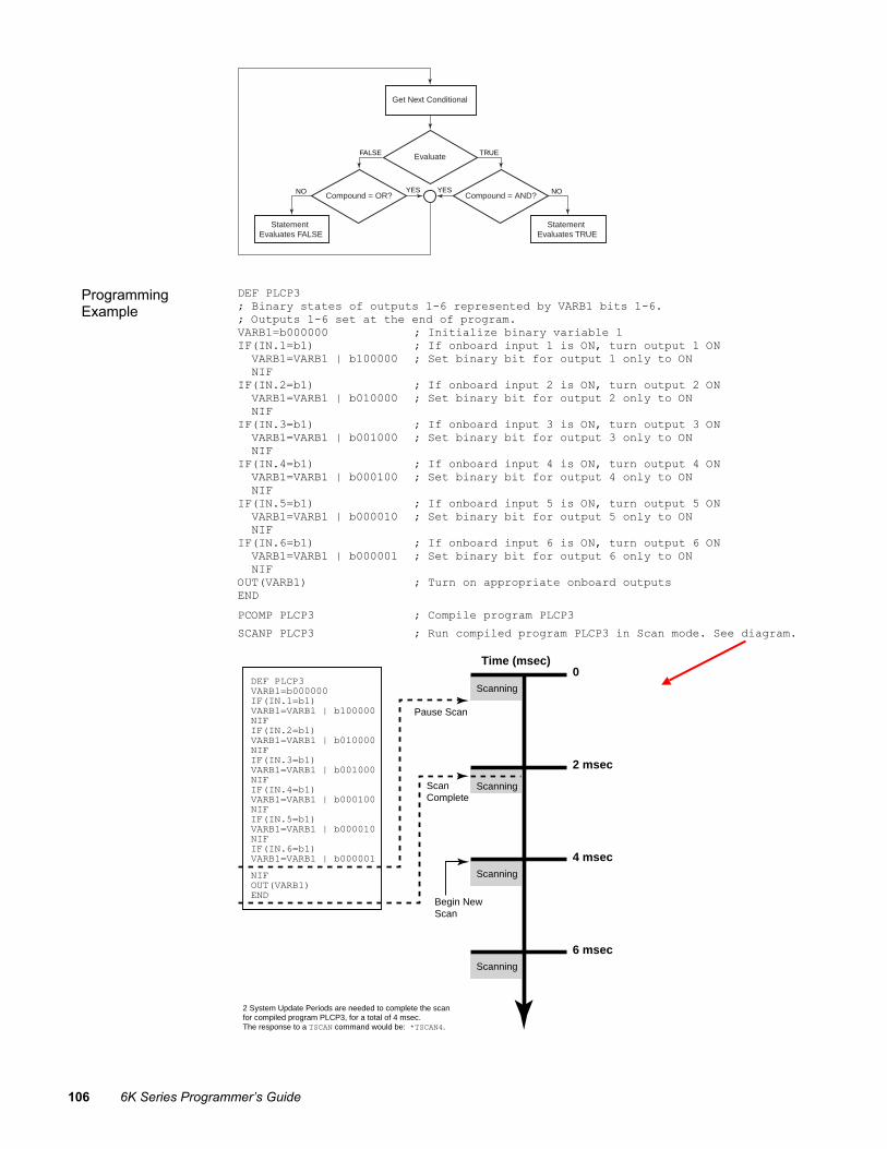
106 6K Series Programmer’s Guide
NO
Evaluate
Compound = AND?Compound = OR?
FALSE
YES YES
TRUE
Get Next Conditional
Statement Evaluates FALSE
NO
Statement Evaluates TRUE
Programming Example
DEF PLCP3 ; Binary states of outputs 1-6 represented by VARB1 bits 1-6. ; Outputs 1-6 set at the end of program. VARB1=b000000 ; Initialize binary variable 1 IF(IN.1=b1) ; If onboard input 1 is ON, turn output 1 ON VARB1=VARB1 | b100000 ; Set binary bit for output 1 only to ON NIF IF(IN.2=b1) ; If onboard input 2 is ON, turn output 2 ON VARB1=VARB1 | b010000 ; Set binary bit for output 2 only to ON NIF IF(IN.3=b1) ; If onboard input 3 is ON, turn output 3 ON VARB1=VARB1 | b001000 ; Set binary bit for output 3 only to ON NIF IF(IN.4=b1) ; If onboard input 4 is ON, turn output 4 ON VARB1=VARB1 | b000100 ; Set binary bit for output 4 only to ON NIF IF(IN.5=b1) ; If onboard input 5 is ON, turn output 5 ON VARB1=VARB1 | b000010 ; Set binary bit for output 5 only to ON NIF IF(IN.6=b1) ; If onboard input 6 is ON, turn output 6 ON VARB1=VARB1 | b000001 ; Set binary bit for output 6 only to ON NIF OUT(VARB1) ; Turn on appropriate onboard outputs END
PCOMP PLCP3 ; Compile program PLCP3
SCANP PLCP3 ; Run compiled program PLCP3 in Scan mode. See diagram.
DEF PLCP3VARB1=b000000IF(IN.1=b1)VARB1=VARB1 | b100000NIFIF(IN.2=b1)VARB1=VARB1 | b010000NIF IF(IN.3=b1)VARB1=VARB1 | b001000NIFIF(IN.4=b1)VARB1=VARB1 | b000100NIFIF(IN.5=b1)VARB1=VARB1 | b000010NIFIF(IN.6=b1)VARB1=VARB1 | b000001
NIFOUT(VARB1)END
Pause Scan
Scanning
Scanning
Scanning
Scanning
Begin NewScan
0
2 msec
Time (msec)
4 msec
6 msec
2 System Update Periods are needed to complete the scanfor compiled program PLCP3, for a total of 4 msec.The response to a TSCAN command would be: *TSCAN4.
Scan Complete

Chapter 4. Product Control Options 107
RP240 Remote Operator Panel 6K Series products are directly compatible with the Compumotor RP240 Remote Operator Panel. This section describes how to use your 6K product with the RP240. Instructions for connecting the RP240 are provided in the 6K Hardware Installation Guide. Refer to the Model RP240 User Guide (p/n 88-012156-01) for information on RP240 hardware specifications, mounting guidelines, environmental considerations, and troubleshooting.
�� � � �� �� �
�����
����
������
��������
��������
��������
��������
�����
����
�
�
�
�
�
�
�
�
����
�
�
�
�
���
�
!
�����
"
#�$
���������������� �� ��������� ��������� ���������������5���������������������������������� �(������-������ ���������5����� ����� ���� ������ ��������� ������������8�������������������&�����������������'����������
$-,����.�� �� �� ������'���������������� ��
�-+3�*-�!$$�������������(������� ���������
��������
���������������� �� ����������� ��9����������������5����� �� ����������������������������� ���� ���������������������������� �������������� ��
���������������� �� ���������� ����#���������(���������������������������� 4����������� �� �� �������������5����� ���#���������(��������������������������� 4������ �������������� �����������5����� ���������� ������������� ��������
�� ������
������������������������� �� � �������������������������� �� �
:%� �4�;<%���������������3�������������� ������������ ������������������' ��������4�������������������� ��������������<=��
3���������&�������������� ���������-����� ��� �&����� �����%�������������� �����(���������� ���������� ���� ������(������������'����������������� ��
3������� ������&��������� ����(������ ����� ��������������������� ���3��������������� ������������� ������(����� ��� �����(�������������������������(������������ �� ����������� �������4����������
>�������"�3����������������������'�����������������?����5���@�� �����������(���� �����(�������� ���3��������������' ����'�����������������?����5���@:�
A���������������*�:;<B���������������������������&���������������������� �������������&�'(�)'%����'*(+�%��(�,'�����'�4��������������������*�:;<B���������� ���������������� ���������4?����������4�� ���C����������(����4��&��������� �������� 4����������� <<<��������������-��%�.�%��*(,/�%���,����'��
Configuration NOTE
As shipped from the factory, your 6K product is configured to operate an RP240 from the RS-232/485 connector (referred to as the “COM 2” port). This should be appropriate for the majority of applications requiring RP240 interface.
For more information on controlling your product's multiple
serial ports, see page 37.
Every 6K Series product has two serial ports. The RS-232 connector is referenced as the “COM1” serial port, and the RS-232/485 connector is referenced as the “COM2” serial port.
To configure the 6K product's serial ports for use with the RP240 and/or 6K language commands, use the DRPCHK command. Be sure to select the affected serial port (COM 1 or COM 2) with the PORT command before you execute the DRPCHK command. Once you issue the DRPCHK command, it is automatically saved in non-volatile memory. The configuration options are:
DRPCHKØ ..........Use the serial port for 6K commands only (default for COM 1) DRPCHK1 ..........Check for RP240 on power up or reset. If detected, initialize RP240.
If no RP240, use serial port for 6K commands. DRPCHK2 ..........Check for RP240 every 5-6 seconds. If detected, initialize RP240. Do not use
port for 6K commands. DRPCHK3 ..........Check for RP240 on power up or reset. If detected, initialize RP240.
If no RP240, use serial port for DWRITE command only. The DWRITE command can be used to transmit text strings to remote RS-232C devices. (default setting for COM 2)

108 6K Series Programmer’s Guide
Example COM 2 is to be used for RS-485; COM 1 is to be used for RP240, but the RP240 will be plugged in on an as-needed basis. The set-up commands for such an application should be executed in the following order: PORT1 ; Select COM1 serial port for setup DRPCHK2 ; Configure COM1 for RP240, periodic check PORT2 ; Select COM2 serial port for setup DRPCHKØ ; Configure COM2 for 6K commands only
Operator Interface Features The RP240 can be used as your product’s operator interface, not a program entry terminal. As an operator interface, the RP240 offers the following features:
• Displays text and variables • 8 LEDs can be used as programmable status lights • Operator data entry of variables: read data from RP240 into variables and command
value substitutions (see Command Value Substitutions on page 7).
Typically the user creates a program in the 6K controller to control the RP240 display and RP240 LEDs. The program can read data and make variable assignments via the RP240's keypad and function keys.
The 6K Series software commands for the RP240 are listed below. Detailed descriptions are provided in the 6K Series Command Reference. The example below demonstrates the majority of these 6K Series commands for the RP240.
DCLEAR............Clear The RP240 Display DJOG................Enter RP240 Jog Mode [DKEY]............Numeric value of RP240 Key DLED................Turn RP240 LEDs On/Off DPASS..............Change RP240 Password DPCUR..............Position The Cursor On The RP240 Display [DREAD] .........Read RP240 Data [DREADF] .......Read RP240 Function Key DREADI............RP240 Data Read Immediate Mode DRPCHK............Check for RP240 DSTP................Enable/Disable the RP240 Stop Key DVAR................Display Variable On RP240 DWRITE............Display Text On The RP240 Display

Chapter 4. Product Control Options 109
Programming Example
DEF panel1 ; Define program panel1 REPEAT ; Start of repeat loop DCLEAR0 ; Clear display DWRITE"SELECT A FUNCTION KEY" ; Display text "SELECT A FUNCTION KEY" DPCUR2,2 ; Move cursor to line 2 column 2 DWRITE"DIST" ; Display text "DIST" DPCUR2,9 ; Move cursor to line 2 column 9 DWRITE"GO" ; Display text "GO" DPCUR2,35 ; Move cursor to line 2 column 35 DWRITE"EXIT" ; Display text "EXIT" VAR1 = DREADF ; Input a function key IF (VAR1=1) ; If function key 1 hit GOSUB panel2 ; GOSUB program panel2 ELSE ; Else IF (VAR1=2) ; If function key 2 hit DLED1 ; Turn on LED 1 GO1 ; Start motion on axis 1 DLED0 ; Turn off LED 1 NIF ; End of IF (VAR1=2) NIF ; End of IF (VAR1=1) UNTIL (VAR1=6) ; Repeat until VAR1=6 (function key 6) DCLEAR0 ; Clear display DWRITE"LAST FUNCTION KEY = F" ; Display text "LAST FUNCTION KEY = F" DVAR1,1,0,0 ; Display variable 1 END ; End of panel1 DEF panel2 ; Define prog panel2 DCLEAR0 ; Clear display DWRITE"ENTER DISTANCE" ; Display text "ENTER DISTANCE" D(DREAD) ; Enter distance number from RP240 END ; End of panel2
Using the Default Menus On power-up, the 6K product will automatically default to a mode in which it controls the RP240 with the menu-driven functions listed below.
The flow chart below illustrates the RP240's menu structure in the default operating mode (when no 6K product user program is controlling the RP240). Press the Menu Recall key to back up to the previous screen. The menu functions are described in detail below.
• Run a stored program (run, stop, pause and continue functions)
• Jog the load
• Display the status of: - System (TSS), for each task - Axis (TAS) - Extended Axis (TASX) - I/O (TIN and TOUT) - Limits (TLIM) and ENABLE input (TINO bit 6) - Position: Commanded (TPC), Encoder (TPE) - Firmware revision levels for the 6K product (TREV) and the RP240
• Enable or disable the internal drive (DRIVE)
• Access RP240 menu functions with a security password (set with DPASS)
• Reset the 6K product (equivalent to the Reset command)
NOTE: To disable these menus, the start-up program (the program assigned with the STARTP command) must contain the DCLEARØ command.

110 6K Series Programmer’s Guide

Chapter 4. Product Control Options 111
Running a Stored Program
������ �� ��������������������������� ����������������������!�����
������� �� ������������������������������
������ ����������"�������������������������������������
������ ����������"�������������������������������������
After accessing the RUN menu, press F1 to “find” the names of the programs stored in the 6K product’s memory; pressing F1 repeatedly displays subsequent programs in the order in which they were stored in BBRAM. To execute the program, press the ENTER key.
To type in a program name at the location of the cursor, first select alpha or numeric characters with the F2 function key (characters will be alpha if an asterisk appears to the right of ALPHA, or numeric if no asterisk appears). If alpha, press the up (2) or down (8) keys to move through the alphabet, if numeric, press the desired number key. Press F3 to move the cursor to the left, or F4 to move the cursor to the right.
Only user programs defined with DEF and END can be executed from this menu. Compiled profiles (contouring and GOBUF profiles) cannot be executed from this men; they must be executed from the terminal emulator with the PRUN command, or you can place the PRUN (name of path) command in a user program and then execute that program from this menu.
HINT: If you wish to display each command as it is executed, select STEP and TRACE and press the
ENTER key to step through the program.
When a program is RUN and TRACE is selected (TRACE*), the RP240 display will trace all program commands as they are executed. This is different from the TRACE command in that the trace output goes to the RP240 display, not to a terminal via the serial port.
When a program is RUN and STEP is selected, step mode has been entered. This is similar to the STEP command, but when selected from the RUN menu the step mode allows single stepping by pressing the ENTER key. Both RP240 trace mode and step mode are exited when program execution is terminated.
Jogging ������ �� ��������������������������� ����������������������!�����
�������"��#�����������������������"��#�����$%&$$$�������������������������� ��' You can jog individual axes by pressing the arrow keys on the RP240’s numeric keypad. Pressing an arrow key on the numeric keypad will start motion and releasing the arrow key will stop motion. The up and down arrows keys are for selecting the axis to jog. The left and right arrow keys are for jogging the selected axis in the negative and positive direction, respectively.
The HI and LO values in the jog menu represent the velocity in units of revs/sec (or volts/sec for ANI feedback). If scaling is enabled, the value is multiplied by the programmed SCLV value.
To edit the jog velocity* values: 1 . Press the F5 function key under EDIT (edit mode indicated with an asterisk). 2 . Press the F1 function key to select the HI and LO values (cursor appears under the
first digit of the value selected). 3 . Using the numeric keyboard, enter the value desired. 4 . Repeat steps 2 and 3 for all values to be changed. 5 . Press ENTER when finished editing. 6 . To jog with the new velocity values, first press the F6 function key (under JOG) to
enable the arrow keys again.
Jog accel and decel values are specified by the JOGA and JOGAD commands, respectively.
or

112 6K Series Programmer’s Guide
Status Reports: System & Axis
��!��� ������������������������������������������
������ �� ��������������������������� ����������������������!�����
��!��� ��������(������"�#����������"�#��$���"��$$$��$$$$$$$$$$$$$$��$$$$$$$$$$
��������������(������"�#����������"�#�����"�$$�$$$$$$$$$�$$$$$$$$$$��$$$$$$$
��������������(������"�#����������"�#������"�$$$$$�$$$$$$$$$$$$$$$$$$$$$$$$$$
After accessing the desired status menu, you can ascertain the function and status of each system (TSS, for each task) or axis (TAS and TASX) status bit by pressing the arrow keys on the numeric keypad.
To view a more descriptive explanation of each status bit (includes a text description), press the left or right arrow keys on the numeric keypad.
Status Reports: I/O, Limits, Position
�$��"����������������#��(�����������"��#���$$$$)$$$$)$$$$)$$$$)$
�$���"���������������#��(�����������"��#���$$$$)$$$$
��� ���"���������������������������"��#���������"����"������"����� �"�����(��"�
������ �� ��������������������������� ����������������������!�����
��� ��"��������������������������"��#����������"�*�
���������������"�������������������"��#����������"�*�
���������"����������� ����������������������������
������!"����������������� ���������������
�$��"����������������#��(�����������"��#���$$$$)$$$$)$$$$)$$$$)$
��������"��������������������������"��#����������"�*�
�������������
INPUTS Menu: This menu displays the TIN bit patterns for programmable inputs (onboard triggers and digital inputs on expansion I/O bricks). Remember that I/O bit patterns vary by product (see page 76 to find the bit patterns for your product). The initial menu show the trigger inputs status; use the up and down arrows to select the status of inputs on expansion I/O bricks.
OUTPUTS Menu: This menu displays the TOUT bit patterns for programmable outputs (onboard outputs and digital outputs on expansion I/O bricks). Remember that I/O bit patterns vary by product (see page 76 to find the bit patterns for your product). The initial menu show the onboard outputs; use the up and down arrows to select the status of outputs on expansion I/O bricks.
LIMITS Menu: • The POS, NEG and HOME status items represent the hardware states of the limit inputs
on the “LIMITS/HOME” connector, regardless of their LIMFNC input function assignments; they do not represent INFNC limit functions assigned to onboard trigger inputs or digital inputs on expansion I/O bricks.
• “POS” refers to the hardware end-of-travel limit imposed when counting in the positive

Chapter 4. Product Control Options 113
direction. “NEG” refers to the limit imposed when counting in the negative direction. • A “1” indicates that the input is grounded, “0” indicates not grounded.
The end-of-travel limits (POS and NEG) must be grounded to allow motion (this is reversed if the active level is reversed with the LHLVL command).
The Enable input (ENABLE input terminal) must also be grounded before motion is allowed. When not grounded, the output (analog voltage or step pulse) to the drives is cut off and the shutdown outputs are activated.
POS Menu: • The position values (encoder, commanded, and position error) shown are continually
updated. • The position error (“ERROR”) report is applicable only to servo axes. • Position values are subject to the SCLD scaling factor (if scaling is enabled—SCALE1),
PSET offset value, encoder polarity (ENCPOL), and commanded direction polarity (CMDDIR).
Enabling and Disabling the Drive(s)
���������"��������������������������"�#��������������
������ �� ��������������������������� ����������������������!�����
In the DRIVE menu, the current status of the drive(s) is displayed. To enable or disable the drive, press F1 or F2, respectively This menu offers the same functionality as the DRIVE command.
WARNING Shutting down a rotary drive system allows the load to freewheel if there is no brake installed.
Access Security
�������++++���,-.�/01123.4�,5-��/.-11������
������� �� ����������������������*(���������������������������������
������ �� ��������������������������� ����������������������!�����
������� �� ������������������������������ ������������������ ���������
����������-��
������������
If the RP240 password is modified with the DPASS command to be other than the default (see Changing the Password below) the ACCESS menu then becomes the new default menu after power-up or executing a RESET. After that, the new password must then be entered to access the original default menu (see “Access Approved” path in illustration). If the operator does not know the new password, all he or she can do is run programs stored in the 6K product (RUN).
Changing the Password: The default password for 6K products is “6000”. A new password (numeric value of up to 4 characters) can be established with the DPASS command. For example, the DPASS2001 command sets the password to 2001.

114 6K Series Programmer’s Guide
Revision Levels
�������"����67*$��8�$*$�*&%$���7�$����"�67*$�76&�*$��
������� �� ����������������������*(���������������������������������
������ �� ��������������������������� ����������������������!�����
Resetting the 6K Product
������� ���������!��������
������� �� ����������������������*(���������������������������������
������ �� ��������������������������� ����������������������!�����
After accessing the RESET menu, press the F1 key to execute a reset (or press F2 to cancel and exit the menu). The reset is identical to issuing a RESET command or cycling power to the 6K product. If a start-up program has been assigned with the STARTP command, that program will be executed.
CAUTION
Executing a reset will restore most command values (exclusions: see page 33) to their factory default setting.
Joystick Control, Analog Inputs
Refer to your
Installation Guide for connection
procedures.
The 6K allows you to add analog input (ANI) SIMs to the expansion I/O bricks (sold separately). Each ANI SIM provides 8 analog inputs. The default voltage range for these input is -10VDC to +10VDC, but other ranges are selectable with the ANIRNG command. ANI inputs can be used in a variety of ways:
• Control an axis with a joystick (see Joystick Control) • Position feedback for servo axes. The position of the ANI inputs can be read using the
PANI or TPANI commands. • Use the voltage value to control other events. The voltage value on the ANI inputs can
be read using the ANI or TANI commands.
Joystick Control The 6K controller supports joystick operation with digital inputs and analog inputs. The digital inputs include the onboard limit inputs and trigger inputs, as well as digital input SIMs on an external I/O brick. The 12-bit analog inputs are available only if you install an analog input SIM on an external I/O brick (default voltage range is -10V to +10V, selectable with ANIRNG).
Chapter 4. Product Control Options 115
To Set Up Joystick Operation (refer also to the example code below)
1. Select the required digital inputs and analog inputs required for joystick operation. Connect the joystick as instructed in your controller’s Installation Guide.
2. Assign the appropriate input functions to the digital inputs used for joystick's operation: • Release Input: INFNCi-M for triggers & I/O brick inputs, or LIMFNCi-M for limit
inputs. • Axis Select Input: INFNCi-N for triggers & I/O brick inputs, or LIMFNCi-N for limit
inputs. NOTE: If you're not using this input, assign the analog inputs to the axes with the JOYAXH command.
• Velocity Select Input: INFNCi-O for triggers & external inputs, or LIMFNCi-O for limit inputs.
3. (optional) Use the ANIRNG command to select the voltage range for the analog inputs you will use. The default range is -10VDC to +10VDC (other options are 0 to +5V, -5 to +5V, and 0 to +10V).
4. Assign analog inputs to control specific axes, using: • JOYAXH: Standard analog input-to-axis assignment. • JOYAXL (optional). Analog input-to-axis assignment when the Axis Select Input is low.
5. Define the joystick motion parameters: • Maximum Velocity when Velocity Select input switch is open/high (JOYVH command).
If the Velocity Select input is not used, joystick motion always uses the JOYVH velocity.
• Maximum Velocity when Velocity Select input switch is closed/low (JOYVL command).
• Accel (JOYA command). • Accel for s-curve profiling (JOYAA command). • Decel (JOYAD command). • Decel for s-curve profiling (JOYADA command).
6. Define the usable voltage zone for your joystick: (make sure you have first assigned the analog inputs – see step 3 above) • End Deadband (JOYEDB): Defines the voltage offset (from the -10V & +10V
endpoints) at which maximum velocity occurs. Default is 0.1V, maxing voltage at -9.9V and +9.9V.
• Center Voltage (JOYCTR or JOYZ): Defines the voltage when the joystick is at rest to be the zero-velocity center. Default JOYCTR setting is 0V.
• Center Deadband (JOYCDB): Defines the zero-velocity range on either side of the Center Voltage. Default is 0.1V, setting the zero-velocity range at -0.1V to +0.1V.
7. To jog the axes: a. In your program, enable Joystick Operation with the JOY command (Joystick Release
input must be closed in order to enable joystick mode). When the JOY command enables joystick mode for the affect axes, program execution stops on those axes (assuming the Continuous Command Execution Mode is disabled with the COMEXCØ command).
b. Move the load with the joystick. c. When you are finished, open the Joystick Release input to disable joystick mode. This
allows program execution to resume with the next statement after the initial JOY command that started the joystick mode.

116 6K Series Programmer’s Guide
Joystick Programming Example (refer also to the illustration below)
Application Requirements: This example represents a typical two-axis joystick application in which a high-velocity range is required to move to a region, then a low-velocity range is required for a fine search. After the search is completed it is necessary to record the load positions, then move to the next region. A digital input can be used to indicate that the position should be read. The Joystick Release input is used to exit the joystick mode and continue with the motion program.
Hardware Configuration: • An analog input SIM is installed in the 3rd slot of I/O brick 1. The eight analog inputs
(1-8) are addressed as input numbers 17-24 on the I/O brick. Analog input 17 will control axis 1, and analog input 18 will control axis 2.
• A digital input SIM is installed in the 1st slot of I/O brick 1. The eight digital inputs (1-8) are addressed as input numbers 1-8 on the I/O brick. Digital input 6 will be used for the Joystick Release function, and input 7 will be used for the Joystick Velocity Select input. Input 8 will be used to indicate that the position should be read.
Setup Code (the drawing below shows the usable voltage configuration):
1INFNC7-M ; Assign Joystick Release f(n) to brick 1, input 7 1INFNC8-O ; Assign Joystick Velocity Select f(n) to brick 1, input 8 JOYAXH1-17,1-18 ; Assign analog input 17 to control axis 1, ; Assign analog input 18 to control axis 2 JOYVH1,1 ; Max. velocity on axes 1 & 2 is 10 units/sec when the ; Velocity Select input (1IN.7) is open (high) JOYVL10,10 ; Max. velocity on axes 1 & 2 is 1 unit/sec when the ; Velocity Select input (1IN.7) is closed (low) JOYA100,100 ; Set joystick accel to 100 units/sec/sec on both axes JOYAD100,100 ; Set joystick decel to 100 units/sec/sec on both axes ;**** COMMANDS TO SET UP USABLE VOLTAGE: ********** 1JOYCTR.17=+1.0 ; Set center voltage for analog input 17 (controls axis 1) 1JOYCTR.18=+1.0 ; and 18 (controls axis 2) to+1.0V. The +1.0V value was ; ascertained by checking the voltage of the both ; inputs (with the 1TANI.17 and 1TAIN.18 commands) ; when the joystick was at rest. 1JOYCDB.17=0.5 ; Set center deadband to compensate for the fact that 1JOYCDB.18=0.5 ; when the joystick is at rest, the voltage received on ; both analog inputs can fluctuate +/- 0.5V on either ; side of the +1.0V center. 1JOYEDB.17=2.0 ; Set end deadband to compensate for the fact that the 1JOYEDB.18=2.0 ; joystick can produce only -8.0V to +8.0V. ;************************************************** JOY11 ; Enable joystick mode for axes 1 & 2
Velocity(positive direction)
Volts
Velocity(negative direction)
-10V +10V
JOYVH or JOYVL
JOYVH or JOYVL
JOYCTR or JOYZ(voltage when joystick is at rest)
JOYCDB(zero-velocity range)
JOYEDB
JOYEDB

Chapter 4. Product Control Options 117
Analog Input Interface
Refer to your product's Installation Guide for
ANI connection information.
Using analog (ANI) inputs on expansion I/O bricks, your 6K Series controller can use analog voltage as position feedback (servo axes only) and simply as a means to control the program based on external conditions.
Each ANI SIM on an expansion I/O brick provides eight analog inputs. The 12-bit analog inputs have a default voltage range of -10VDC to +10VDC. Other ranges are selectable with the ANIRNG command (0 to +5VDC, 0 to +10VDC, and -5 to +5VDC). The voltage value of the ANI inputs can be transferred to the terminal with the TANI command, or used in an assignment or comparison operation with the ANI operator (e.g., IF(1ANI<2.4)).
When used for position feedback, the position counter resolution is 205 counts/volt (under the default ANIRNG setting). The position value of the ANI inputs can be transferred to the terminal with the TPANI command, or used in an assignment or comparison operation with the PANI operator (e.g., WAIT(1PANI>421)).
Three common applications of the ANI inputs are: • Position command to the control loop (e.g., as a master axis in Following mode) • Position feedback to the control loop (see page 67 to select ANI input feedback for
servo axes) • A force or torque feedback signal
Programming Example
The portion of 6K code below (for two axes of control) demonstrates how to read the analog inputs into the controller and set the commanded analog output of each axis to that value. If you have a torque drive, this provides open-loop torque control. SGP0,0 ; Turn off servo proportional feedback gain SGI0,0 ; Turn off servo integral feedback gain SGV0,0 ; Turn off servo velocity feedback gain SGAF0,0 ; Turn off servo acceleration feedforward gain SGVF0,0 ; Turn off servo velocity feedforward gain SOFFS0,0 ; Set offset to zero (analog output will be 0 volts) L ; Enter an infinite loop VAR1=2ANI.17 ; Read value of 1st analog input on SIM slot 3
; (I/O point 17) on I/O brick 2 on into VAR variable 1 VAR1=2ANI.18 ; Read value of 2nd analog input on SIM slot 3
; (I/O point 18) on I/O brick 2 on into VAR variable 2 SOFFS(VAR1),(VAR2) ; Assign voltages from 2ANI.17 and 2ANI.18 to the ; analog output for axes 1 & 2, respectively T.01 ; Set time delay to 10 milliseconds LN ; End loop
ANI as a Feedback Device
The ANI analog inputs, when selected as a feedback source with the SFB command, is assumed to provide position information. With this feedback it is possible to solve applications that require positioning to a voltage, rather than positioning to a known position. Some example applications are as follows:
• Using a potentiometer as feedback (mechanical motion is mimicked by the 6K controller)
• Maintaining a force while position changes due to fluid evacuating a chamber • Opening or closing a valve as another process changes

118 6K Series Programmer’s Guide
Host Computer Interface
Another choice for product control is to use a host computer and execute a motion program using the serial interface (RS-232 or RS-485). A host computer can be used to run a motion program interactively from a BASIC or C program (high-level program controls the 6K product and acts as a user interface). A BASIC program example (for the 6K2 product) is provided below.
10 ' 6K Series Serial Communication BASIC Routine 12 ' 6K.BAS 14 ' 16 ' ************************************************************** 18 ' 20 ' This program will set the communications parameters for the 22 ' serial port on a PC to communicate with a 6K series 24 ' stand-alone product. 26 ' 28 ' ************************************************************** 30 ' 100 '*** open com port 1 at 9600 baud, no parity, 8 data bits, 1 stop bit 110 '*** activate Request to Send (RS), suppress Clear to Send (CS), suppress 120 '*** DATA set ready (DS), and suppress Carrier Detect (CD) *** 130 OPEN "COM1:9600,N,8,1,RS,CS,DS,CD" FOR RANDOM AS 1 140 ' 150 '*** initialize variables *** 160 MOVE$ = "" ' *** commands to be sent to the product *** 170 RESPONSE$ = "" ' *** response from the product *** 180 POSITION$ = "" ' *** feedback position reported *** 190 SETUP$ = "" ' *** setup commands *** 200 ' 210 '*** format the screen and wait for the user to start the program *** 220 CLS : LOCATE 12, 20 230 PRINT "Press any key to start the program" 240 ' 250 '*** wait for the user to press a key *** 260 PRESS$ = INKEY$ 270 IF PRESS$ = "" THEN 260 280 CLS 290 ' 300 '*** set a pre-defined move to make *** 310 SETUP$ = "ECHO1:ERRLVL0:LH0,0:" 320 MOVE$ = "A100,100:V2,2:D50000,50000:GO11:TFB:" 330 ' 340 ' 400 '*** send the commands to the product *** 410 PRINT #1, SETUP$ 420 PRINT #1, MOVE$ 430 ' 500 ' *** read the response from the TFB command *** 510 ' *** the controller will send a leading "+" or "-" in response to the TFB command to 520 ' *** indicate which direction travel has occurred. *** 530 WHILE (RESPONSE$ <> "+" AND RESPONSE$ <> "-") ' *** this loop waits for the "+" 540 RESPONSE$ = INPUT$(1, #1) ' *** or "-" characters to be returned 550 WEND ' *** before reading the position *** 560 ' 570 WHILE (RESPONSE$ <> CHR$(13)) ' *** this loop reads one character at a time 580 POSITION$ = POSITION$ + RESPONSE$ ' *** from the serial buffer until a carriage 590 RESPONSE$ = INPUT$(1, #1) ' *** return is encountered *** 600 WEND 610 ' 620 '*** print the response to the screen *** 630 LOCATE 12, 20: PRINT "Position is " + POSITION$ 640 ' 650 'END

5C H A P T E R F I V E
CustomProfiling
IN THIS CHAPTER
This chapter explains how to use these custom profiling features: • S-Curve Profiling ..............................................120 • Linear Interpolation...........................................123 • Contouring (circular interpolation) ...................124 • Compiled Motion Profiling ...............................136 • On-the-Fly Motion (pre-emptive GOs) ..............151 • Registration .......................................................155 • Synchronizing Motion.......................................159
For basic motion (accel/velocity/distance), see page 53. For homing profiles, see page 59. For Following profiles, see page 166.

120 6K Series Programmer’s Guide
S-Curve Profiling 6K controllers allow you to perform S-curve move profiles, in addition to the usual trapezoidal profiles. S-curve profiling provides smoother motion control by reducing the jerk (rate of change) in acceleration and deceleration portions of the move profile (see drawing below). Because S-curve profiling reduces jerk, it improves position tracking performance, especially in linear interpolation applications (not contouring).
Dec
elA
ccel
Time
Dec
elV
eloc
ity
Time
Trapezoidal
Acc
el
Time
Vel
ocity
Time
S-Curve
Maximum Jerk Less Jerk
S-Curve Programming Requirements To program an S-curve profile, you must use the average accel/decel commands provided in the 6K Series programming language. For every maximum accel/decel command (e.g., A, AD, HOMA, HOMAD, JOGA, JOGAD, etc.) there is an average command for S-curve profiling (see table below).
Maximum Accel/Decel Commands Command Function
Average (“S-Curve”) Accel/Decel Commands Command Function
A Acceleration AA Average Acceleration AD Deceleration ADA Average Deceleration HOMA Home Acceleration HOMAA Average Home Acceleration HOMAD Home Deceleration HOMADA Average Home Deceleration JOGA Jog Acceleration JOGAA Average Jog Acceleration JOGAD Jog Deceleration JOGADA Average Jog Deceleration JOYA Joystick Acceleration JOYAA Average Joystick Acceleration JOYAD Joystick Deceleration JOYADA Average Joystick Deceleration LHAD Hard Limit Deceleration LHADA Average Hard Limit Deceleration LSAD Soft Limit Deceleration LSADA Average Soft Limit Deceleration PA Path Acceleration PAA Average Path Acceleration PAD Path Deceleration PADA Average Path Deceleration
Determining the S-Curve Characteristics The command values for average accel/decel (AA, ADA, etc.) and maximum accel/decel (A, AD, etc.) determine the characteristics of the S-curve. To smooth the accel/decel ramps, you must enter average accel/decel command values that satisfy the equation ½ A ≤ AA < A, where A represents maximum accel/decel and AA represents average accel/decel. Given this requirement, the following conditions are possible:

Chapter 5. Custom Profiling 121
Acceleration Setting Profiling Condition
AA > ½ A, but AA < A.............S-curve profile with a variable period of constant acceleration. Increasing the AA value above the pure S-curve level (AA > ½ A), the time required to reach the target velocity and the target distance is decreased. However, increasing AA also increases jerk.
AA = ½ A ................................Pure S-curve (no period of constant acceleration—smoothest motion).
AA = A .................................... Trapezoidal profile (but can be changed to an S-curve by specifying a new AA value less than A).
AA < ½ A; or AA > A...............When you issue the GO command, the move will not be executed and an error message, *INVALID CONDITIONS FOR S_CURVE ACCELERATION—FIELD n, will be displayed.
AA = zero................................S-curve profiling is disabled. Trapezoidal profiling is enabled. AA tracks A. (Track means the command's value will match the other command's value and will continue to match whatever the other command's value is set to.) However, if you enter an average decel command (e.g., ADA, HOMADA, etc.) equal to zero, you will receive the “INVALID DATA-FIELD n” error.
AA ≠ zero and AA ≠ A ............S-curve profiling is enabled only for standard moves (e.g., not for contouring, compiled motion, or on-the-fly motion changes). All subsequent standard moves for that axis must comply with this equation: ½ A ≤ AA < A.
AA > ½ A ................................Average accel/decel is raised above the pure S-curve level; this decreases the time required to reach the target velocity and distance. However, increasing AA also increases jerk. After increasing AA, you can reduce jerk by increasing A, but be aware that increasing A requires a greater torque to achieve the commanded velocity at the mid-point of the acceleration profile.
No AA value ever entered ......Profile will default to trapezoidal. AA tracks A.
If you never change the A or AA deceleration commands, AA deceleration will track AA acceleration. However, once you change A deceleration, AA deceleration will no longer track changes in AA acceleration. For example, if you never change the AD or ADA command values, ADA will track the AA command value. But once you change AD, the ADA command value will no longer track the changes in the AA command value.
The calculation for determining S-curve average accel and decel move times is as follows (calculation method identical for S-curve and trapezoidal moves):
Time = VelocityA
or Time = 2 DistanceAavg avg
∗
Scaling affects the AA average acceleration (AA, ADA, etc.) the same as it does for the A maximum acceleration (A, AD, etc.). See page 48 for details on scaling.
NOTE: Equations for calculating jerk are provided on page 122.
Programming Example ; In this example, axis 1 executes a pure S-curve and takes 1 second ; to reach a velocity of 5 rps; axis 2 executes a trapezoidal profile ; and takes 0.5 seconds to reach a velocity of 5 rps. SCALE0 ; Disable scaling DEF SCURV ; Begin definition of program SCURV @MA0 ; Select incremental positioning mode @D40000 ; Set distances to 40,000 positive- ; direction steps A10,10 ; Set max. accel to 10 rev/sec/sec ; on axes 1 and 2 AA5,10 ; Set avg. accel to 5 rev/sec/sec on ; axis 1, & 10 rev/sec/sec on axis 2 AD10,10 ; Set max. decel to 10 rev/sec/sec ; on axes 1 and 2 ADA5,10 ; Set avg. decel to 5 rev/sec/sec on ; axis 1, & 10 rev/sec/sec on axis 2 V5,5 ; Set velocity to 5 rps on axes 1 & 2 GO11 ; Execute motion on axes 1 and 2 END ; End definition of program
Axis 1V
T1 2 30
Axis 2V
T1 2 30
Move profiles

122 6K Series Programmer’s Guide
Calculating Jerk
V2
A(Programmed Accel)
V(Programmed Velocity)
V1
t1 t2 t3
Zero Velocity
Zero Acceleration
Ø(zero)
A B C
Rules of Motion:
dt
Jerk da=
dt
a dv=
dt
v dx= (x = distance)
Assuming the accel profile starts when the load is at zero velocity and the ramp to the programmed velocity is not compromised:
A2 * AA
V (A-AA) Jerk = JA =
A = programmed acceleration
(A, AD, HOMAD, etc.) AA = average acceleration
(AA, ADA, HOMAA, etc.) V = programmed velocity
(V, HOMV, etc.)
A
JA t1 =
V
AA - t2 =
A
JA V
AA t3 =
NOTE: t3 - t2 = t1
2
JA * t12
V1 = 2 * JA
A2 =
V2 = V -
2 * JA
A2
A t1 ≥ t ≥ Ø a (t) = JA * t
2
JA * t2
v (t) =
6
JA * t3
d (t) =
B t2 ≥ t > t1 a (t) = A
2JA
A2 v (t) = + A * (t - t1)
6
JA * t13
d (t) = + + V1 * (t - t1) 2
A * (t - t1)2
C t3 ≥ t > t2 a (t) = A - (JA * (t - t2)) v (t) = V -
2
JA * (t3 - t)2
2AA
V2 d (t) = + - V * (t3 - t)
6
JA (t3 - t)3
Starting at a Non-Zero Velocity: If starting the acceleration profile with a non-zero initial velocity, the move comprises two components: a constant velocity component, and an s-curve component. Typically, the change of velocity should be used in the S-curve calculations. Thus, in the calculations above, you would substitute “(VF - VO)” for “V” (VF = final velocity, VO = initial velocity). For example, the jerk equation would be:
A2 * AA
(VF - VO) (A-AA) Jerk = JA =
a (t) = acceleration at time t v (t) = velocity at time t d (t) = distance at time t

Chapter 5. Custom Profiling 123
Linear Interpolation
NOTE 2-axis products can accommodate only 2-axis (X & Y) linear interpolation.
The controller allows you to perform linear interpolation, the process of moving two or three orthogonal (right angle) linear axes to achieve linear (straight line) motion; a fourth axis can also participate in the move profile. The task is to derive appropriate move parameters to move from a current location to a new location, where each position is specified by a set of Cartesian coordinates. All axes must start, accelerate, decelerate, and stop in a synchronized manner.
The Initiate Linear Interpolated Motion (GOL) command initiates linear interpolation moves based on the parameters set with the D, PA, PAD, and PV commands. You simply enter the desired path acceleration (PA), the path deceleration (PAD), and the path velocity (PV) to arrive at the point in space (end point) specified with the distance (D) command; the controller internally calculates each axis' actual move profiles to achieve a straight-line path with these parameters.
You can scale the acceleration, velocity, and distance with the SCLD command (see example below).
The GOL command starts motion on either or both axes. If the GOL command is issued without any arguments, motion will be started on both axes.
Code Sample SCALE1 ; Enable scaling @SCLD4000 ; Set distance, accel/decel, and velocity scale factor ; to 4000 steps/unit PA25 ; Set the path acceleration to 25 units/sec/sec PAD20 ; Set the path deceleration to 20 units/sec/sec PV2 ; Set the path velocity to 2 units/sec D10,5 ; Set the distance to 10 & 5 units on axes 1 & 2 GOL11 ; Initiate linear interpolated motion on axes 1 & 2 ; (see drawings below)
A���!5���:�
D���!5�����
8
;
E
:
�
� : E ; 8 � F = �< �� �: �E
����
���
���
�-��('%����'&)/(��0%�(�.
0�����
.���
�)��'(��-��%�)�-)�%�')*-/��%)*%�1��%�%2%�)%�+.-�3�%�.�%�-��('%����'&)/(��0%�(�.
!5����
!5���:

124 6K Series Programmer’s Guide
Contouring (Circular Interpolation)
NOTE 2-axis products can accommodate only 2-axis (X & Y) contouring.
6K Series controllers allow you to define and execute two-dimensional motion paths. A path refers to the path traveled by the load in an X-Y plane, and must be defined before any motion takes place along that path. The X and Y axes can be specified as any of the controller's two axes
Controllers with ≥4 axes: A third axis, labeled the C axis, can be included to keep an angular position that changes linearly with the path direction. The path direction is the vector addition of the travel of axes X and Y. A fourth axis labeled the P axis can be included to keep a position that is proportional to the distance traveled along the path described by X and Y. The X, Y, C and P axes can be specified as any of the controller's four axes.
A path consists of one or more line or arc segments whose end-points are specified in terms of X and Y positions. The end-point position specifications can be made using either absolute or incremental programming. The segments can be lines or arcs, both of which are described in greater detail in the following sections. Each path segment is determined by the end-point coordinates, and in the case of arcs, by the direction and radius or center. It is possible to accelerate, decelerate or travel at constant velocity (feedrate) during any type of segment, even between segments. For each segment, the user can also specify an output pattern that can be applied to the programmable outputs at the beginning of that segment.
All paths are continuous paths, (i.e., the motion will not stop between path segments, but must stop at the end of a path). It is not possible to define a path that stops motion within the path definition and then continues that path. To achieve this result, two individual paths must be defined and executed. A path can, however, be stopped and resumed by using a Pause/Continue input (see page 83) while the path is executing. In this case, motion will be decelerated and resumed along the path without loss of position. If one axis is stopped due to any other reason, the other axis will stop abruptly, and motion cannot be resumed. Causes for motion being stopped can include encountering an end-of-travel limit, issuing a Kill (!K) command, detecting a stall (stepper axes), exceeding the maximum allowable position error (servo axes), etc.
Path Definition
Compiled GOBUF
segments and PLCP programs are also stored
in compiled memory (see page 11).
Contouring paths are defined like programs (using the DEF and END commands), but are compiled with the PCOMP command and executed with the PRUN command. Programs intended to be compiled as paths are stored in Program memory. After they are compiled with the PCOMP command, they remain in program memory and the segments (PARCM, PARCOM, PARCOP, PARCP, and PLIN statements) from the compiled profile are stored in Compiled memory. The TDIR command reports which programs are stored as a compiled profile.
The amount of RAM allocated for storing contouring path segments is determined by the MEMORY command setting. The list below identifies memory allocation defaults and limits for 6K Series products. Further details on re-allocating memory are provided on page 11.
Total memory (bytes) ......................................... 300,000 Default allocation (program,compiled) ..............MEMORY150000,150000 Maximum allocation for compiled profiles ........MEMORY1000,299000 Maximum No. of compiled profiles ................... 300 Maximum No. of compiled profile segments ..... 2069
CAUTION Issuing a memory allocation command (e.g., MEMORY70000,80000) will erase all existing programs and compiled contouring path segments. However, issuing the MEMORY command by itself (i.e., MEMORY—to request the status of how the memory is allocated) will not affect existing programs or path segments.

Chapter 5. Custom Profiling 125
You can store the maximum number of paths possible (see table above) as long as each path has at least one segment, and the sum of all the segments of all the paths does not exceed the controller's compiled memory limitation. All path definitions can be compiled and ready to execute at any time. Paths defined using 6K commands are specified with a path name. Once a path definition is compiled, it can be executed repeatedly without being re-compiled.
Deleting (DEL) an existing path name will automatically delete the existing path compilation with that name. The PUCOMP command only deletes (“uncompiles”) the path compilation, not the path program.
Example Code In the example commands below, storage space is made available for the definition of path WID3 by first deleting the compiled version of paths WID1 and WID2. The DEF statement begins the definition of the path WID3. PUCOMP WID1 ; Remove compilation of WID1 PUCOMP WID2 ; Remove compilation of WID2 DEF WID3 ; Begin definition of WID3
Participating Axes Units of Measure; Scaling
• If no scaling (SCALE0): Path acceleration, velocity, and distance are based on the resolution (DRES for steppers, ERES for servos) of axis 1. If multi-tasking is used, path motion units are based on the resolution of the first (lowest number) axis associated with the task (TSKAX).
• If scaling (SCALE1): The units used for path distance, acceleration, and velocity is determined by the SCLD value. For example, suppose you have 2 servo axes (axes 1 & 2) involved in contouring, both axes use encoder feedback with a resolution of 4000 counts/rev, axis 1 uses a 10:1 (10 turns per inch) leadscrew and axis 2 uses a 5:1 (5 turns per inch) lead screw, and you want to program in inches. For this application you would use the SCLD40000,20000 command to establish path motion units in inches: distance is inches, acceleration is inches/sec/sec, and velocity is inches/sec.
2-Axis Contouring You can change the X-Y plane to an Y-X plane by using the PAXES command. A path definition default is PAXES1,2. For any path that uses axis 2 as the X axis and axis 1 as the Y axis, the path definition must start with PAXES2,1 (see example below).
Example Code DEF DRAW1 ; Begin definition of DRAW1 PAXES2,1 ; Set contouring axes (axis 2 is X axis, axis 1 is Y axis)
4-Axis Contouring Some contouring applications can require the execution of more than one path to complete a part or finish an operation. The application can require that different paths take place in different planes of a three dimensional work area. In addition, some of the paths can require a third axis to move either tangent, or proportional to the path. For these reasons, a four-axis controller offers great flexibility in the specification of participating axes.
You may want to begin your path definition with the PAXES command; this will ensure that you have specified the appropriate axes to participate in the path. The X, Y, tangent (C) and proportional (P) axes can be specified as any of the four axes, and this specification must be made before any of the path travel specifications are made. The X and Y axes must be specified, the third (tangent) axis labeled C and the fourth (proportional) axis labeled P are optional.
The C axis will maintain an angular position that changes linearly with the direction of travel in the X-Y plane. This allows the C axis to control an object, which must stay tangent (or normal) to the direction of travel such as a cutting tool. The C axis must also be specified by its signed resolution. The magnitude of the resolution is the number of C axis motor steps in 360 degrees of an arc drawn by the X and Y axes. The sign of the resolution specifies the direction of rotation of the C axis. Refer to the PTAN command.

126 6K Series Programmer’s Guide
�
D
A
The P axis will keep a position that is proportional to the distance traveled along the X-Y path as the path is executed. This allows the P axis to act as the Z axis in helical interpolation (see drawing at left), or to control the motion of any object that moves with distance and velocity proportional to the path. The P axis must also be specified by the signed ratio of P axis travel to path travel. The magnitude of this ratio can range from 0.001 to 1000. The sign of this ratio specifies the direction of rotation of the P axis. Refer to the PPRO command.
A sewing machine application can require all four axes (X, Y, C, and P). The X and Y axes would direct the sewing head along the required path. The C axis would keep the sewing head pointed into the direction of travel. The P axis would control the speed of the needle, so that an even stitch is made, regardless of path speed.
Example Code The following example begins the definition of a path named DRAW1. The X and Y axes are specified to be axes 4 and 2. The path includes the C axis to be axis 1, with a resolution of 100,000 steps. It also includes the P axis to be axis 3, with a ratio of P axis travel to path travel specified as 2.5:1. DEF DRAW1 ; Begin definition of DRAW1 PAXES4,2,1,3 ; Set contouring axes PTAN100000 ; Define C axis resolution PPRO2.5 ; Define P axis ratio
Path Acceleration, Deceleration, and Velocity A path can be composed of many segments, each with their own motion parameters. The path velocity, acceleration, and deceleration specifications currently in effect at the time a segment is defined will apply to that segment. This allows construction of a path that moves at one velocity for a section of the path, then moves at a different velocity for another section.
In most cases, it will be desirable to maintain a constant velocity throughout the path, but it is easy to define a path in which each segment has its own velocity. For example, this can be useful when a tool needs to slow down to round a corner, or to allow the rate of glue application to be controlled by the path speed. Acceleration and deceleration can also be specified separately.
Example Code The short code example below illustrates the specification of velocity, acceleration, and deceleration in that order. Note that the scaling commands cannot be placed inside a program.
PV0.5 ; Path velocity 10,000 counts/sec PA16 ; Path acceleration 400,000 counts/sec/sec PAD28 ; Path deceleration 700,000 counts/sec/sec
Path Final Velocity The PVF command allows a line or arc segment to terminate with a final segment velocity (PVF) that can be different from the velocity traveled for the majority of that segment (specified with PV). PVF must be smaller than or equal to PV, and the path velocity change will take place at the PAD deceleration rate. Like the other path motion parameters (e.g., PV, PA, PAD), the PVF velocity is applied to the next line or arc compiled; however, unlike these other commands, the PVF command applies only to the next line or arc compiled. All subsequent lines and arcs terminate at the PV value currently in effect. For each line or arc that needs to terminate at a velocity different than PV, a new PVF command must be issued, even if the PVF value has not changed.
The most common use for the PVF command will be to cause a preceding line segment to decelerate to the path velocity at which the next line or arc needs to travel. In this case, the PVF value for the preceding line would be the same as the PV value of the reduced speed segment. This feature eliminates the need to create a special deceleration segment in the path in order to have the entire subsequent line or arc travel at the reduced speed.

Chapter 5. Custom Profiling 127
Example Code In the example below, segments 2 and 4 must travel at a path velocity of 1, while the remainder to the path travels at a path velocity of 5.
Segment 1 Segment 2 Segment 3Segment 4
Segment 5
DEF CORNERPAB1 ; Use absolute positionsPA10 ; Path acceleration of 10PAD10 ; Path deceleration of 10PV5 ; Starting path velocity of 5PVF1 ; Ending segment velocity of 1PLIN5,0 ; 5 units right (Segment 1)PV1 ; Path segment velocity of 1PLIN6,0 ; Another unit right, slowly (Segment 2)PV5 ; Starting path velocity of 5PVF1 ; Ending segment velocity of 1PLIN11,0 ; 5 more units right (Segment 3)PV1 ; Path segment velocity of 1PARCM12,1,1 ; Upward arc slowly (Segment 4)PV5 ; Starting path velocity of 5PLIN12,6 ; 5 units up (Segment 5)END
Conditional Path Execution The PGOWHN command allows a fixed or conditional delay in path travel to occur as part of the contouring motion profile, without requiring program execution to monitor the PGOWHN conditions. Combined with the PVF command, PGOWHN provides a convenient method of imbedding a dwell within a contour.
���������� ����
*����� ��-5������� ��� ��5"
�������������������������������������������������
��������2��������"
������� .������������������������� # ������������������� ,'���� ������� ���
��������2��������"
�������
��������2��������"
G +������(���������� ���������
G ,������ ��� �G 7� ����(�����!""""����������� �����������
The PGOWHN expression can be specified as a time (dwell) in milliseconds (e.g., PGOWHN(T=2000)), or as inputs or limits matching the specified binary pattern (e.g., PGOWHN(LIM.3=B1) or PGOWHN(2IN.6=B0)). All participating axes will be at rest during a dwell, even if the previous segment had not ended in zero path velocity. In the latter case (limit or input condition), there will be an abrupt change to zero path velocity, until the PGOWHN condition is satisfied.
When the PGOWHN condition is satisfied, path velocity will ramp to the next segment’s PV value. Although no motion occurs during a PGOWHN segment, it occupies one segment of compiled memory. Like the line and arc segments, an output pattern can be asserted for the duration of the PGOWHN dwell by preceding the PGOWHN statement with a POUT statement (see example below).

128 6K Series Programmer’s Guide
Example Code In the example below, the total path travel is six inches. At five inches, motion must stop until input 3 goes active. During this time, output 2 must be asserted. When input 3 goes active, output 2 must go off and motion then resumes for the final inch. DEF BISEG PAB1 ; Use absolute positions PA10 ; Path acceleration of 10 PAD10 ; Path deceleration of 10 PV5 ; Starting path velocity of 5 PVF0 ; Ending segment velocity of 0 POUT.2-0 ; Start with onboard output 2 off PLIN5,0 ; 5 units right POUT.2-1 ; Output 2 on during dwell PGOWHN(IN.3=B1) ; Dwell until onboard input 3 is active POUT.2-0 ; Output 2 off during motion PLIN6,0 ; Another unit right to finish END
Segment End-point Coordinates Stepper axes: All end-
point position specifications are in units of commanded
counts.
The end-point position specifications of lines and arcs can be either absolute or incremental. The controller stores the end-point data for all of its compiled segments internally as incremental, relative to the start of the segment. But in order to ease the programming task, absolute coordinates and multiple coordinate systems can be used.
When incremental coordinates are used to specify an end-point, the X and Y end-point values represent the distances from the X and Y start point of the segment being specified. Center specifications of an arc are always incremental (i.e., relative to the start of that arc segment). When absolute coordinates are used to specify an end-point, the X and Y end-point values represent that segment's position in the specified coordinate system. Incremental and absolute programming are specified with the PAB command. Incremental programming is the default state at the beginning of a path definition.
Coordinate systems allow the assignment of an arbitrary X-Y position as a reference position for subsequent absolute end-point specifications. The controller allows the use of two coordinate systems for use with absolute coordinate programming. These are called the Work coordinate system and the Local coordinate system. These are specified with the PWC and PLC commands. Neither coordinate system needs to represent the actual absolute position of the axes when the path actually executes.
The Work and Local coordinate systems are provided to allow absolute end-point definition of a segment without needing to know the actual position of each axis when the segment is executed. If no PWC command precedes the first segment command when a path definition begins, the controller will place the start of the first segment at location (0,0) in the Work coordinate system. By using the PWC xpos,ypos command, the programmer defines subsequent absolute end-points to refer to the Work coordinate system, and also locates that coordinate system such that the starting position of the next segment is at (xpos, ypos) of the Work coordinate system.
The Local coordinate system is provided so that if a section of a path is to appear in multiple locations along the path, the segments that compose that section can be programmed in absolute coordinates. By using the PLC xpos,ypos command, the programmer defines subsequent absolute end-points to refer to the Local coordinate system, and also locates that coordinate system such that the starting position of the next segment is at (xpos, ypos) of the Local coordinate system.
A single path definition can include both absolute and incremental programming, and be required to switch between Work and Local coordinates several times. At any point along a path definition, coordinates can be switched from absolute to incremental, or from incremental to absolute. When switching to absolute, all subsequent end-point specifications are assumed to be absolute with respect to the coordinate system in effect at that time. This

Chapter 5. Custom Profiling 129
remains true until the reference system is switched to incremental, or to a new absolute reference.
When switching from Work coordinates to Local coordinates, the Local X and Y start positions of the following segment must be specified with the PLC command. When starting a path definition with Work coordinates, or when switching to Work coordinates, the starting position of the next segment can either be specified or assumed. The controller toggles between the Work coordinate system and the Local coordinate system with the PL command.
Ease of programming results from the ability to switch between absolute and incremental, and to re-define the coordinate systems between sections of a path. This allows individual sections of path definition to have Local coordinate systems, yet still be integrated into the complete path.
Line Segments
Lines are the simpler of the two path segment types. The placement, length, and orientation of the line is completely specified by the end-point of the line segment and the end-point of the previous segment. As described above, end-points can be specified with absolute or incremental coordinates.
8<<<
F <D
A
�<4<�
�F <48<<<�
The example below is specified with incremental coordinates and results in a line segment 10,000 steps in length, at 30 degrees in the X-Y plane. PLIN8660,5000 ; Line segment to (8660,5000) — see illustration at left
Arc Segments
A�!5��
=<H
�F<H
:�<H
�
�
# ����� �,������
�
�
<H���E <H
Arcs are more complex to specify than lines, because there are four possible ways to get from the start point to the end point. The radius of an arc can either be specified directly or implied by the center specification. In the controller, all path descriptions refer to the X-Y plane. The general convention describing the X-Y plane, as viewed from a drawing, is as follows. The X axis is shown as the left-right axis, with left being negative and right being positive. The Y axis is the up-down axis with down being negative and up being positive. Angles start at zero and increase in the CCW direction of rotation. A line segment, or the radius of an arc is at zero degrees if the incremental end-point has a positive X component and zero Y component. The angle is 90 degrees if the end-point has a positive Y component and zero X component.
Radius Tolerance Specifications
All arcs have an associated radius. In the controller, the radius can either be specified explicitly, or implied by a center specification. In both cases, it is possible that the radius cannot be consistent with the specified end-point of the arc. This could be a result of improper specification, user calculation error, or of round-off error in the internal arithmetic of the controller. For this reason, the controller allows the specification of a radius tolerance (PRTOL). The radius tolerance is specified in the same units as the radius and X and Y data.
The radius tolerance has a factory default of ± one step, which is just enough to overcome round-off errors. The radius tolerance can be specified at any point along the path definition, and can be changed between one arc and the next. Each arc definition will be compared to the most recently specified radius tolerance. The radius tolerance should be about the same as the dimension tolerances of the finished product. The following paragraphs explain how the radius tolerance is used for the two types of arc specifications, and gives syntax examples for the radius tolerance specification.

130 6K Series Programmer’s Guide
Radius Specified Arcs
*
- �%��� �
�����
Specification of an arc using the radius method requires knowledge of the start point, the end point, and the sign and magnitude of the radius. The controller knows the start point to be either the start of the path, or the end of the previous segment. The end point and radius are provided by the user's program. It is possible to specify an impossible arc by specifying an end point that is more than twice the radius away from the start point (see drawing at left). In this case, the controller will automatically extend the radius to reach the end-point, provided that the automatic radius change does not exceed the user specified radius tolerance. If the required radius extension exceeds the radius tolerance, the controller will respond with an execution error, and no arc will be generated.
Example The following illustration shows the four possible ways to move from the start point to the end point using an arc of radius 1000. Arc 1 and 2 both travel in the CW direction, arc 3 and 4 both travel in the CCW direction. Arc 1 and 3 are both less than 180 degrees. An arc of 180 degrees or less is specified with a positive radius. Arc 2 and 4 are both greater than 180 degrees. An arc of more than 180 degrees is specified with a negative radius. The example code below shows the radius tolerance specification and the specifications of arcs 1, 2, 3, and 4 respectively.
DEF arcs ; Begin definition of path arcs PRTOL5 ; 5 steps of radius tolerance PARCP866,500,1000 ; Arc 1, CW < 180 degrees PARCP866,500,-1000 ; Arc 2, CW > 180 degrees PARCM866,500,1000 ; Arc 3, CCW < 180 degrees PARCM866,500,-1000 ; Arc 4, CCW > 180 degrees END ; End path definition ;*********************************************** ;* To compile the arcs path, type "PCOMP arcs" * ;* To run the arcs path, type "PRUN arcs" * ;***********************************************
��I�<<<
�<4�<<<�
!��:
��I��<<<
!��;
- ����� ��F 48<<�
��������� ��<4<�
!���
!��E
Center Specified Arcs
��������� ��<4<�
- ����� ���8<48<�
*�I�<��
*�I��<<
�� �����<<4<�
Specifying an arc, using the center method, requires knowledge of the start point, the end point, and the center point of the arc. The X coordinate of the center is referred to with the letter I, and the Y coordinate of the center is referred to with the letter J. When an arc is specified with the center, another potential problem arises.
It is possible to specify the center of an arc such that the radius implied by the start point does not equal the radius implied by the end point (see illustration on left). In this case, the controller will re-locate the center so that the resulting arc has a uniform radius and the starting and ending angles come as close as possible to those implied by the user's center specification. This automatic center relocation will take place only if the start point and end point radius difference does not exceed the user specified radius tolerance. If the radius tolerance is exceeded, an execute error will result, and the arc will not be included in the path.
While automatic center relocation will ensure a continuous path, it can result in an abrupt change in path direction. This happens because a new location for the center results in a new tangent direction for an arc about that center.
Example The example code below shows the specifications of arcs 1, 2, 3, and 4 for the drawing on the right. In the 6K commands, the order of the data is X, Y, I, J from left to right. DEF arcs2 ; Begin definition of path PARCOP866,500,866,-500 ; Arc 1, CW < 180 degrees PARCOP866,500,0,1000 ; Arc 2, CW > 180 degrees PARCOM866,500,0,1000 ; Arc 3, CCW < 180 degrees PARCOM866,500,866,-500 ; Arc 4, CCW > 180 degrees END ; End path definition ;************************************************* ;* To compile the arcs2 path, type "PCOMP arcs2" * ;* To run the arcs2 path, type "PRUN arcs2" * ;*************************************************
��I�<<<
�<4�<<<�
!��:
��I��<<<
!��;
- ����� ��F 48<<�
��������� ��<4<�
!���
!��E

Chapter 5. Custom Profiling 131
Circles A circle is a special case of an arc whose end-point is the same as the starting point. Because these two points are the same, it is impossible to determine the location of the circle's center from a radius specification. For this reason, an arc that is a complete circle must be specified using the arc center specification method. An arc with identical starting and ending points specified with the radius method will be ignored. The circle shown below is specified with the example below.
Example DEF circle ; Begin definition of path circle PARCOP0,0,0,500 ; Circle with center at (0,500) END ; End path definition ;*************************************************** ;* To compile the circle path, type "PCOMP circle" * ;* To run the circle path, type "PRUN circle" * ;***************************************************
�� ����<48<<�
�������/���������
�0�0�
Segment Boundary So far, all the examples given have shown isolated line or arc segments. Most paths will consist of many segments put together. The point at which the segments are connected is called a segment boundary in this text. The controller automatically ensures that the path is continuous, in that segments are placed end-to-end.
The path velocity can either be constant or change from segment to segment, according to user specification. Velocity changes use the specified acceleration and deceleration and can take place even across segment boundaries.
The programmer should ensure that direction of travel is also continuous across segment boundaries (see Figure A). If the direction change is abrupt (as shown in Figure B) the X and Y axes will suffer abrupt acceleration or deceleration. The controller ensures that there will be no abrupt direction change within a segment, but the programmer is responsible for ensuring that the direction is continuous across segment boundaries. At low speeds, some motor and mechanical configurations will tolerate such abrupt changes, and the controller will accept such a program; however, it is generally good practice to design paths with smooth direction changes. This can be done by designing a path using arcs to round corners.
A
D
D�0�
.���
A
D
D�0�
.���
����������
Figure A (Segment Example) Figure B (Stall Example for stepper axis)
Using the C Axis (products with ≥4 axes) The C axis is an axis whose position changes in a manner linearly related to the direction of travel in X and Y (i.e., the path direction). The C axis would be used in applications that require a work piece or tool to remain tangent or perpendicular to the path direction. Examples would be: a knife always pointing into the cut, or a welding head staying normal to the weld.
The magnitude of the C axis resolution refers to the number of steps of C axis position change for 360 degrees of direction change in the X-Y plane. This number can be the same as, or different from the C axis motor resolution, allowing any gearing that is convenient for the mechanics. If the C axis load is to be driven directly, the C axis resolution should be the same as the C axis motor resolution. This will cause the C axis motor and load to rotate once when a circle is drawn by the X and Y axes. If the C axis load is to be geared (e.g., 5:1), the C axis resolution specifications should be five times the C axis motor resolution. This will cause the actual motor to rotate five times and the load to rotate once when a circle is drawn by the X and Y axes.

132 6K Series Programmer’s Guide
The number can be positive or negative, allowing greater flexibility in C axis motor mounting orientation. If the sign is positive, the C axis will rotate in the positive direction when CCW arcs are drawn. If the sign is negative, the C axis will rotate in the negative direction when counter-clockwise arcs are drawn.
The C axis is assumed to be in the proper position when path execution begins. It will change position only as the direction of travel changes. The program must position the C axis before the path is executed. This can be done with the HOM command or a GO to a position.
Because the C axis position changes linearly with the direction of X-Y travel, it is important to avoid path definitions that result in an abrupt direction change between segments. The segment boundary considerations for the C axis are similar to those for the X and Y axes, except that abrupt direction changes will result in abrupt C axis position changes. The X and Y axis would only suffer large accelerations, which can cause a stall in stepper axes or exceed the maximum position error (SMPER value) in servo axes. The C axis will suffer impossibly high velocity commands, causing stall and position loss in steppers or position error in servos.
Using the P Axis (products with ≥4 axes) The P axis is an axis whose position and velocity are proportional to the position and velocity traveled by the load along the path generated by X and Y. It can be used as the Z axis in helical interpolation, or to control other motion that must be proportional to the X-Y path motion. The proportionality of the P axis is specified as a ratio, with a range of ±0.001 to ±1000. The sign of the ratio determines which direction the motor will turn. The magnitude specifies the ratio of P axis travel to path travel, regardless of path direction or segment type. This ratio is essentially a position ratio, but because the ratio is maintained at every instant it also becomes a velocity ratio.
The P axis only responds to the distance traveled along the path, and is not affected by direction changes in the path. The only caution that must be observed comes when a high ratio is specified. In this case, path velocity and acceleration are amplified, which can result in impossible velocities or stalls (stepper axes) or excessive position error (servo axes).
Outputs Along the Path For each segment, you can also specify an output pattern (POUT), which is to be applied to the programmable outputs at the beginning of that segment and remains throughout that segment. These segment-defined output patterns are stored as part of the compiled path definition. These outputs will change state at some time between 1.5 ms before the beginning of the segment and 0.5 ms after the beginning of the segment. The programmable outputs cannot be controlled more precisely than this, because the controller updates its path position every 2 ms.
The path segment defined programmable outputs are provided so that plotting applications can raise and lower the pen, laser cutters can turn the laser on and off, glue applicators can be turned on and off, all at prescribed positions along the path. The output specification is stated before the segment definition, which holds that output state. In the example below, programmable outputs 2 and 4 are changed during the path segments.
Example Code
DEF prog1 ; Begin definition of path program prog1 POUT1001 ; Output pattern during first arc PARCM5,5,5 ; Specify incremental X-Y endpoint position and
; radius arc <180° for 1/4 circle CCW arc POUT1100 ; Output pattern during second arc
PARCM5,-5,-5 ; Specify incremental X-Y endpoint ; position and radius arc >180° for ; 3/4 circle CW arc END ; End definition of prog1 PCOMP prog1 ; Compile path program prog1 PRUN prog1 ; Execute path program prog1 OUT0000 ; Turn off programmable outputs 1-4
�����$$�
������$$
���$$$$
Paths Built Using 6K Series Commands
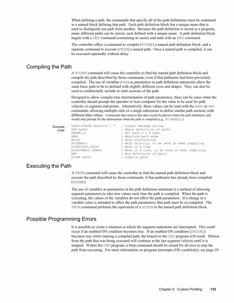
Chapter 5. Custom Profiling 133
When defining a path, the commands that specify all of the path definitions must be contained in a named block defining that path. Each path definition block has a unique name that is used to distinguish one path from another. Because the path definition is stored as a program, many different paths can be stored, each defined with a unique name. A path definition block begins with a DEF command (containing its name) and ends with an END command.
The controller offers a command to compile (PCOMP) a named path definition block, and a separate command to execute (PRUN) a named path. Once a named path is compiled, it can be executed repeatedly without delay.
Compiling the Path A PCOMP command will cause the controller to find the named path definition block and compile the path described by those commands, even if that pathname had been previously compiled. The use of variables (VAR) as parameters in path definition statements allow the same basic path to be re-defined with slightly different sizes and shapes. They can also be used to conditionally include or omit sections of the path.
Designed to allow compile-time determination of path parameters, there can be cases when the controller should prompt the operator or host computer for the value to be used for path velocity or segment end-points. Alternatively, these values can be read with the READ or DAT commands, allowing multiple calls of a single subroutine to define similar path sections with different data values. Commands that retrieve this data would be placed within the path definition, and would only prompt for the information when the path is compiled (e.g., PV(READ1)).
Example Code
VARS1="PATH VELOCITY ? " ; Create message string DEF path1 ; Begin definition of path1 PAXES1,2 ; Set path X & Y axes PAB1 ; Absolute path mode PA100 ; Path acceleration PV(READ1) ; Path velocity, to be read in when compiling PLIN25000,25000 ; Move in a line PLIN(VAR2),(VAR3) ; Move in a line, to be read in when compiling END ; End definition of path1 PCOMP path1 ; Compile path1
Executing the Path A PRUN command will cause the controller to find the named path definition block and execute the path described by those commands, if that pathname has already been compiled (PCOMP).
The use of variables as parameters in the path definition statement is a method of allowing segment parameters to take new values each time the path is compiled. When the path is executing, the values of the variables do not affect the path parameters. If a change in a variable value is intended to affect the path parameters, that path must be re-compiled. The PRUN command performs the equivalent of a GOSUB to the named path definition block.
Possible Programming Errors It is possible to create a situation in which the segment statements are interrupted. This could occur if an enabled ON condition becomes true. If an enabled ON condition (ONCOND) becomes true while running a compiled path, the branch to the ONP program will result. Motion from the path that was being executed will continue at the last segment velocity until it is stopped. Within the ONP program, a Stop command should be issued for all axes to stop the path from executing. For more information on program interrupts (ON conditions), see page 29.

134 6K Series Programmer’s Guide
Programming Examples Figure A and Figure B show two simple paths that illustrate most of the controller segment types. For both figures, axis 1 is X and axis 2 is Y. The C and P axes are not included.
Figure A specifies the end-points with absolute coordinates. The default Work coordinate system with start point of (0,0) is used, so no PLØ statement is needed.
Figure B specifies the end-points with incremental coordinates. The state of the programmable outputs needs to be different for Handles than for Knobs. No other controller actions take place during these paths.
6K Code DEF HANDLE ; Begin HANDLE path definition PAXES1,2 ; Set X axis as axis 1, and ; set Y axis as axis 2 PAB1 ; Use absolute coordinates POUT1100 ; Programmable pattern for ; next segments PARCOM10,10,0,10 ; CCW quarter circle PLIN10,20 ; Vertical LINE segment PARCP20,10,-10 ; CW 3/4 circle PARCM20,0,5 ; CCW half circle END ; End of HANDLE path definition DEF KNOB ; Begin KNOB path definition PAXES1,2 ; Set X axis to be axis 1, and ; set Y axis to be axis 2 PAB0 ; Use incremental coordinates POUT0011 ; Programmable pattern for next ; segments PLIN30,0 ; Long LINE into circular knob PARCOM0,0,0,10 ; CCW circle for the knob PLIN10,0 ; Short LINE out of knob END ; End of KNOB path definition
*�I��<
*�I�8
��<4:<�
��<4�<�
�<4<� �:<4<�
�:<4�<�
Figure A (HANDLE Example)
*�I��<
�E<4<� Figure A (KNOB Example)
The third path consists of two pairs of the first two (see drawing below). Each pair is placed at variable locations within the Work coordinate system and the two pairs are connected with a Line segment. The Line leading into the first pair starts at (20,20) in the Work coordinate system. The first pair starts at (VAR1,2Ø) and the second pair starts at (VAR2,2Ø) in the Work coordinate system. Handle is defined using the Local coordinate system. Even though Handle is defined in absolute coordinates and appears in two different places along the path in PARTS, the statements describing it appear only once, in a path definition using local coordinates.

Chapter 5. Custom Profiling 135
6K Code DEF PARTS ; Begin PARTS path definition PAXES1,2 ; Set X axis to be axis 1, Y axis to be axis 2 PAB1 ; Use absolute coordinates PWC20,20 ; Establish WORK coordinates PL0 ; Enable WORK coordinates PLIN(VAR1),20 ; LINE to (VAR1,20) PLC0,0 ; Specify LOCAL coordinate system PL1 ; Enable LOCAL coordinate system PAB1 ; Use absolute coordinates POUT1100 ; Programmable pattern for next segments PARCOM10,10,0,10 ; CCW quarter circle PLIN10,20 ; Vertical LINE segment PARCP20,10,-10 ; CW 3/4 circle PARCM20,0,5 ; CCW half circle PAB0 ; Use incremental coordinates POUT0011 ; Programmable pattern for next segments PLIN30,0 ; Long LINE into circular knob PARCOM0,0,0,10 ; CCW circle for the knob PLIN10,0 ; Short LINE out of knob PAB1 ; Use absolute coordinates PL0 ; Return to WORK coordinates PLIN(VAR2),20 ; LINE to (VAR2,20) PLC0,0 ; Specify LOCAL coordinate system PL1 ; Enable LOCAL coordinate system PAB1 ; Use absolute coordinates POUT1100 ; Programmable pattern for next segments PARCOM10,10,0,10 ; CCW quarter circle PLIN10,20 ; Vertical LINE segment PARCP20,10,-10 ; CW 3/4 circle PARCM20,0,5 ; CCW half circle PAB0 ; Use incremental coordinates POUT0011 ; Programmable pattern for next segments PLIN30,0 ; Long LINE into circular knob PARCOM0,0,0,10 ; CCW circle for the knob PLIN10,0 ; Short LINE out of knob END ; End of PARTS path definition PCOMP PARTS ; Compile PARTS path definition
*�I��<
*�I�8
*�I��<
�E<4<�
:<
0!*� 0!*::<
/��&������� ����������
*�I��<
*�I�8
*�I��<
�E<4<�

136 6K Series Programmer’s Guide
Compiled Motion Profiling 6K Series products allow you to construct complex motion profiles for each individual axis. The profiles can contain:
• Sequences of motion • Loops • Programmable output changes • Embedded dwells • Direction changes • Trigger functions
Related Commands: Brief descriptions of related commands are found on page 136. For detailed descriptions, see the 6K Series Command Reference.
Contouring path
segments and PLCP programs are also stored
in compiled memory (see page 11).
Compiled motion profiles are defined like programs (using the DEF and END commands); the commands used to construct the motion profile segments are stored in a program (stored in Program memory). This program is then compiled (using the PCOMP command) and the compiled profile segments (GOBUF, PLOOP, GOWHEN, TRGFN, POUTA, POUTB, POUTC, and POUTD statements) from the program are stored in Compiled memory. (HINT: The TDIR command reports which programs are compiled as a compiled profile.) You can then execute the compiled profile with the PRUN command.
The amount of RAM allocated for storing compiled profile segments is determined by the MEMORY command setting. The list below identifies memory allocation defaults and limits for 6K Series products. Further details on re-allocating memory are provided on page 11.
Total memory (bytes) ......................................... 300,000 Default allocation (program,compiled) ..............MEMORY150000,150000 Maximum allocation for compiled profiles ........MEMORY1000,299000 Maximum No. of compiled profiles ................... 300 Maximum No. of compiled profile segments ..... 2069
CAUTIONS
• Issuing a memory allocation command (e.g., MEMORY70000,230000) will erase all existing programs and compiled path segments. However, issuing the MEMORY command by itself (i.e., MEMORY—to request the status of how the memory is allocated) will not affect existing programs or segments.
• After compiling (PCOMP) and running (PRUN) a compiled profile. The profile segments will be deleted from compiled memory if you cycle power or issue a RESET command.
After compiling (PCOMP), you can execute the profiles with the PRUN command, and all of the motion and functions compiled into the profile are executed without any further commands during profile execution.
For multi-axis products, profiles on any combination of axes can be launched simultaneously with a single PRUN command. This provides a very powerful method of synchronizing the action of multiple axes with very simple programming. For example, in a four-axis product, one axis could be running a complex Following profile, while two other axes are contouring, and the fourth could be performing a multi-tiered velocity motion profile.
Because the motion and functions are pre-compiled, delays associated with command processing are eliminated during profile execution, allowing more rapid sequencing of actions than would be possible with programs that are not compiled. Command processing is then free to monitor other activities, such as I/O and communications.

Chapter 5. Custom Profiling 137
NOTES • During compilation (PCOMP), most commands are executed the same as if no profile were being
defined, even those that are not relevant to the construction of a profile. This is also true of non-compiled motion commands embedded in a compiled motion program during PCOMP. For this reason, it’s good to limit commands between DEF and END to those that actually assist in the construction of the profile. Even for those that do actually assist in the construction of the profile, such as A, V, and D, it is important to remember that the command is executed and data actually changes, and it is not restored after compilation is completed.
• If your compiled motion program contains variables, the variables are evaluation only at compile time.
Each motion segment in a compiled motion profile can have its own distance, velocity, acceleration, and deceleration, as shown in the program example below:
Programming Example
DEF simple ; Begin definition of program simple MC0 ; Preset positioning mode (disable continuous mode) D50000 ; Distance is 50000 A10 ; Acceleration is 10 AD10 ; Deceleration is 10 V5 ; Velocity is 5 GOBUF1 ; Store the first motion segment for axis 1. ; Profile attributes are: MC0, A10, AD10, V5, D50000 D30000 ; Distance is 30000 V2 ; Velocity is 2 GOBUF1 ; Store the second motion segment for axis 1 ; Profile attributes are: MC0, A10, AD10, V2, D30000 D40000 ; Distance is 40000 V4 ; Velocity is 4 GOBUF1 ; Store the third motion segment for axis 1 ; Profile attributes are: MC0, A10, AD10, V4, D40000 ; Because this is the last segment in a preset profile, ; the velocity will automatically end at zero. END ; End program definition PCOMP simple ; Compile simple PRUN simple ; Run simple The resulting profile from the above program:
v
t0
1
2
3
4
5
D50000
D30000D40000
STATUS COMMANDS Use these commands to check the status of compiled profiles.
System Status (TSSF, TSS, & SS): • Bit 29 is set if compiled memory is 75% full. • Bit 30 is set if compiled memory is 100% full. • Bit 31 is set if a compile (PCOMP) failed; this bit is cleared on power-up, reset, or after a
successful compile. Possible causes include: - Errors in profile design (e.g., change direction while at non-zero velocity, distance
& velocity equate to <1 count/system update, preset move profile ends in non-zero velocity).
- Profile will cause a Following error (see TFS, TFSF & FS status). - Out of memory (see system status bit 30) - Axis already in motion at the time of the PCOMP command - Loop programming errors (e.g., no matching PLOOP or PLN, more than 4
embedded PLOOP/END loops)
Axis Status (TASF, TAS, & AS): Bit 31 is set while compiled a GOBUF profile is executing.

138 6K Series Programmer’s Guide
TSEG & SEG: Reports the number of available segments in compiled memory.
TDIR: Identifies programs that are “compiled as a path” (compiled with the PCOMP command) and reports the percentage of remaining compiled memory.
Rules for Using Velocity in Preset Compiled Motion
When defining preset mode (MC0) compiled profiles there are several rules that govern the velocity.
Rule 1: The last segment in the compiled profile will automatically end at zero velocity (only if not in a PLOOP/PLN loop).
DEF PROF5 ; Begin definition of profile 5 MC0 ; Select preset positioning V1 ; Set velocity to 1 rev/sec D4000 ; Set distance to 4000 GOBUF1 ; First motion segment (V1, D4000) V2 ; Set velocity to 2 (second segment) GOBUF1 ; Second motion segment (V2, D4000) END ; End definition of profile 5 PCOMP ; Compile profile 5 ; When you execute PRUN PROF5, the resulting profile is:
V
D4000
0
1
2
8000
Rule 2: If you wish intermediate segments to end in zero velocity, use the VF0 command in the respective GOBUF segment.
DEF PROF6 ; Begin definition of profile 6 MC0 ; Select preset positioning V1 ; Set velocity to 1 rev/sec VF0 ; End this segment at zero velocity D4000 ; Set distance to 4000 GOBUF1 ; First motion segment (V1, D4000, VF0) V2 ; Set velocity to 2 (second segment) VF0 ; End this segment at zero velocity GOBUF1 ; Second motion segment (V2, D4000, VF0) END ; End definition of profile 6 PCOMP ; Compile profile 6 ; When you execute PRUN PROF6, the resulting profile is:
V
D4000
0
1
2
8000
Rule 3: CAUTION: With compiled loops (PLOOP and PLN), the last segment within the loop must end at zero velocity or there must be a final segment placed outside the loop. Otherwise, when the profile is compiled with PCOMP you’ll receive the “ERROR: MOTION ENDS IN NON-ZERO VELOCITY–AXIS n” error message and system status bit 31 will be set. after the final segment is completed, the motor will continue moving at the last segment’s velocity.
DEF PROF7 ; Begin definition of profile 7 MC0 ; Select preset positioning D3000 ; Set distance to 3000 PLOOP4 ; Loop (between PLOOP & PLN) 4 times V1 ; Set velocity to 1 rev/sec GOBUF1 ; First motion segment PLN1 ; End loop END ; End definition of profile 7 PCOMP ; Compile profile 7, but instead of compile, you receive ; an error message

Chapter 5. Custom Profiling 139
To fix the profile, reduce the PLOOP count by one and add a GOBUF statement after the PLN command: DEF PROF7 ; Begin definition of profile 7 MC0 ; Select preset positioning D3000 ; Set distance to 3000 PLOOP3 ; Loop (between PLOOP & PLN) 3 times V1 ; Set velocity to 1 rev/sec GOBUF1 ; Looped motion segment PLN1 ; End loop GOBUF1 ; Last motion segment (end at zero velocity) END ; End definition of profile 7 PCOMP ; Compile profile 7 ; When you execute PRUN PROF7, the resulting profile is:
V
D3000
0
1
2
6000 120009000
Rule 4: With compiled loops (PLOOP and PLN), if you wish the velocity at the end of each loop to end at zero, use a VF0 command.
DEF PROF8 ; Begin definition of profile 8 MC0 ; Select preset positioning D3000 ; Set distance to 3000 PLOOP4 ; Loop (between PLOOP & PLN) 4 times V1 ; Set velocity to 1 rev/sec VF0 ; End each segment at zero velocity GOBUF1 ; Looped motion segment PLN1 ; End loop END ; End definition of profile 8 PCOMP ; Compile profile 8 ; When you execute PRUN PROF8, the resulting profile is:
V
D3000
0
1
2
6000 120009000
Compiled Following Profiles
More details on Following are found in Chapter 6 (page 166).
The new FOLRNF command designates that the motor will move the load the distance designated in a preset GOBUF segment, completing the move at the specified final ratio. The only allowable value for FOLRNF is zero (0). FOLRNF is allowed for a segment only if the starting ratio is also zero, i.e., it must be the first segment, or the previous segment must have ended in zero ratio. FOLRNF is only useful with compiled preset Following moves because the starting and final ratios are already zero for motion initiated with GO.
Compiled motion profiles can be constructed with any combination of preset or continuous motion segments. A continuous (MC1) Following segment will start with the final ratio of the previous segment, and end with the ratio given by FOLRN and FOLRD. The motion segment will consist of one ramp from the starting ratio to the final ratio. Just as with continuous Following ramps outside of a compiled profile, the master travel over which the ramp takes place is specified with FOLMD. The slave travel over which the ramp takes place is simply the product of master travel and average ratio. Because the slave travel is not specified explicitly, it is possible for arithmetic round-off errors to cause actual slave travel during a ramp to differ

140 6K Series Programmer’s Guide
from theoretical calculations. For applications in which slave distance is important, preset segments should be used.
A preset (MCØ) Following segment will also start with the final ratio of the previous segment, but can end in one of two ways. FOLRNF specifies the final ratio of a preset Following segment. As previously described, the only valid value for FOLRNF is zero (0). If FOLRNFØ is given before the GOBUF, the resulting motion segment will be constructed exactly as preset Following moves are outside of compiled profiles. In this case, the starting ratio must be zero, the final ratio will be zero, and the maximum intermediate ratio will be given by FOLRN and FOLRD. The relationships between ratio, master distance, and slave distance for this case are given on page 195 under the heading Master and Follower Distance Calculations. The FOLRNF command affects only the immediately subsequent preset Following segment, and must be given explicitly for each preset segment that is to end in zero ratio.
If FOLRNFØ is not given before the GOBUF, the segment will end with the ratio given by FOLRN and FOLRD, and need not start with zero ratio. This type of motion segment is constrained, however, to intermediate ratios that fall between the starting and final ratios.
Compiled profiles are built from motion segments created with the GOBUF command. For each individual axis, all motion segments in a compiled profile must use the same state of Following. That is, the motion segments can be all Following or all non-Following, but not a mixture of Following and non-Following (but at any point in time, separate axes can have different Following mode states).
The GOBUF command builds the appropriate type of motion segment based on the values of FOLMAS and FOLEN during compilation. These parameters cannot be changed inside a compiled program after a GOBUF. The choice of zero or non-zero FOLMAS must be the same during PRUN as during PCOMP (if non-zero, the value can be changed, but still must be non-zero). If a non-zero FOLMAS is given, the value of FOLEN must be the same during PRUN as during PCOMP.
Distance Calculations For Compiled Following Moves
The graph below shows 6 possibilities of ratio change profiles for preset segments, with legal FOLMD and “D” values constrained by the requirement that the average ratio (given by “D”/FOLMD) is between R1 and R2. If the distance is outside these ranges, in the profile used to get from R1 to R2 over FOLMD (covering “D” slave distance), an error message will be generated during the PCOMP command. For the graphs shown, the constraints are expressed by:
(R1 * FOLMD) <= “D” <= (R2 * FOLMD) if R2 > R1 (R1 * FOLMD) >= “D” >= (R2 * FOLMD) if R2 < R1
�� ��
*�
*:
��(��,���� �
,�J��*��K�*:��L��� ��C:
,�I��*��K�*:��L��� ��C:
,�M��*��K�*:��L��� ��C:
�� ��
*�
*:
��(��,���� �
,�M��*��K�*:��L��� ��C:
,�I��*��K�*:��L��� ��C:
,�J��*��K�*:��L��� ��C:

Chapter 5. Custom Profiling 141
The two graphs above show the cases of R1<R2 or R1>R2, but the distance calculations of the ramp and constant ratio portions are the same for the two cases. For each graph, the heavy lined profile (first case) of these mimics the shape of the corresponding preset velocity change (FOLENØ) segments in that the ramp takes place before the constant ratio portion. The second case occurs only if the distance specified exactly matches the start and end ratios and FOLMD1. In the third case, the ramp takes place after the constant ratio portion. In the first and third cases, only two segments are built, and the slave and master distances traveled in each segment are easily calculated with the simple formulas shown below. These formulas are based on positive ratios and master and slave distances. In the construction of Following profiles, ratios and master distances are always positive, with direction implied by the sign of the slave distance. For calculations with negative slave distances, simply use the magnitude of “D” in the formulas below, and invert the sign of the resulting slave distances.
Case 1 (Ramp first) MD1 = [D-(R2*FOLMD)]/((R1-R2)/2) where MD1 = master distance during ramp MD2 = FOLMD - MD1 where MD2 = master distance during flat D1 = .5*(R1+R2)*MD1 where D1 = slave distance during ramp D2 = D - D1 where D2 = slave distance during flat
Case 2 (Ramp only) MD1 = FOLMD where MD1 = master distance during ramp D1 = D where D1 = slave distance during ramp
Case 3 (Ramp last) MD1 = [D-(R1*FOLMD)]/((R2-R1)/2) where MD1 = master distance during ramp MD2 = FOLMD - MD1 where MD2 = master distance during flat D1 = .5*(R1+R2)*MD1 where D1 = slave distance during ramp D2 = D - D1 where D2 = slave distance during flat
Dwells and Direction Changes Compiled profiles can incorporate changes in direction only if the preceding motion segment has come to rest. This can be achieved for non-Following segments either by creating a continuous segment with a goal velocity of zero, or by preceding a preset segment with VFØ. It can be achieved for Following segments either by creating a continuous or preset segment with a goal ratio of zero, or by preceding a preset segment with FOLRNFØ. In all cases, motion within the profile comes to rest, although the profile is not yet complete. Even though the motor is not moving, the axis status bit 1 (AS.1) will remain set, indicating a profile is still underway. Only then can you change direction (using the D+ or D- command, D~ is not allowed) within a profile. An attempt to incorporate changes in direction if the preceding motion segment has not come to rest will result in a compilation error.
In many applications, it can be useful to create a time delay between moves. For example, a machine cycle can require a move out, dwell for 2 seconds, and move back. To create this dwell, a compiled GOWHEN can be used between the two moves. The code within a compiled program can look like: MC0 ; Preset incremental positioning used D(VAR1) ; Target position is in VAR1 VF0 ; Motion comes to rest at end of move GOBUF1 ; Create move out segment GOWHEN(T=2000) ; Profile delays for 2 seconds D- ; Return position is home (direction reversed) VF0 ; Motion comes to rest at end of move GOBUF1 ; Create move back home segment
In Following applications, it can be more useful to create a master travel delay between moves. For example, a machine cycle replacing a cam can require a move out, dwell for 2000

142 6K Series Programmer’s Guide
master counts, and move back. To create this dwell, a compiled GOBUF of zero slave distance can be used between the two moves. The code within a compiled program can look like: MC0 ; Preset incremental positioning used D(VAR1) ; Target position is in VAR1 FOLMD4000 ; Move takes place over 4000 master counts FOLRNF0 ; Motion comes to rest at end of move GOBUF1 ; Create move out segment D0 ; No change in target position FOLMD2000 ; Dwell takes place over 2000 master counts FOLRNF0 ; Motion comes to rest at end of “move” (dwell) GOBUF1 ; Create dwell segment D(VAR1) ; Return position is home (direction change implied) D- ; Return position is home (direction reversed) FOLMD4000 ; Move takes place over 4000 master counts FOLRNF0 ; Motion comes to rest at end of move GOBUF1 ; Create move back home segment
Compiled Motion Versus On-The-Fly Motion The two basic ways of creating a complex profile are with compiled motion or with on-the-fly pre-emptive GO commands. With compiled motion, portions of a profile are built piece by piece, and stored for later execution. Compiled motion is appropriate for profiles with motion segments of pre-determined velocity, acceleration and distance. Compiled motion profiles allow for shorter motion segments, which results in faster cycle times because there is no command processing and execution delay. The axes can perform their own motion control and coordination, freeing program flow for other tasks, such as I/O, machine control, and host requests. The disadvantages to pre-defined compiled motion profiles are the amount of memory use and limited run-time decision making and I/O processing.
With pre-emptive GO moves, the motion profile underway is pre-empted with a new profile when a new GO command is issued. The new GO command constructs and launches the pre-empting profile. Pre-emptive GOs are appropriate when the desired motion parameters are not known until motion is already underway.
The table below summarizes the differences between the use of compiled motion and on-the-fly motion.
Command/Issue Compiled Motion On-The-Fly Motion GOBUF Constructs motion segment and appends to
previously constructed segment N/A
PRUN Used to launch previously compiled motion N/A GO GO causes move during PCOMP GO Constructs & launches profile,
even if moving Direction changes Only if previous motion segment comes to rest
(MCØ & VFØ or MC1 & VØ), else compile error Not allowed during motion, else AS.3Ø, ER.1Ø
Insufficient room for AD (decel) value
Same as on-the-fly Decel is modified (steppers); Motion is killed, AS.3Ø (servos)
Related Commands GOBUF Store a Motion Segment in Compiled Memory:
The GOBUF command creates a motion segment as part of a profile and places it in a segment of compiled memory, to be executed after all previous GOBUF motion segments have been executed. An individual axis profile is constructed by sequentially appending motion segments using GOBUF commands. Each motion segment can have its own distance to travel, velocity, acceleration, and deceleration.
The end of a GOBUF motion segment in preset mode is determined by the distance or position specified. The end of a GOBUF motion segment in continuous mode is determined by the goal velocity specified. In both cases, the final velocity and position achieved by a segment will be the starting velocity and position for the next segment. If either type of segment is followed by

Chapter 5. Custom Profiling 143
a GOWHEN command, the segment’s final velocity will be maintained until the GOWHEN condition becomes true.
PLOOP & PLN Loop Start & Loop End (Compiled Motion only):
The PLOOP and PLN commands specify the beginning and end of an axis-specific profile loop, respectively. All segments defined between the PLOOP and PLN commands are included within that loop.
VF & FOLRNF Final Velocity & Numerator of Slave-to-Master Final Ratio:
The VF and FOLRNF commands are used to designate that the motor will move the load the distance designated in a preset GOBUF motion segment, completing the move at a final speed of zero. The VF command is used when the Following mode is disabled (FOLENØ). The FOLRNF command is used when the Following mode is enabled (FOLEN1).
GOWHEN Conditional GO:
When GOWHEN is compiled in a profile, the GOWHEN condition is stored as part of that profile instead of being executed immediately. When progress through the profile reaches the compiled GOWHEN, AS.26 is set, and the next segment’s execution will be suspended until the GOWHEN condition becomes true. This allows subsequent GOWHEN and GOBUF combinations to be issued and stored, instead of overriding each other.
TRGFN Trigger Functions:
When TRGFN is compiled in a profile, the TRGFN condition is stored as part of that profile instead of being executed immediately. When progress through the profile reaches the compiled TRGFN, the embedded trigger functions are assigned to that trigger. AS.26 is set if the GOWHEN function has been assigned to the trigger, and the next segment’s execution will be suspended until the specified trigger input goes active. This allows subsequent TRGFN, GOWHEN, and GOBUF combinations to be issued and stored, instead of overriding each other.
PCOMP, PRUN & PUCOMP
Compile a Program, Run a Compiled Program, & Un-Compile a Compiled Program:
The PCOMP, PRUN, and PUCOMP commands allow you to incorporate individual axis profiles within compiled motion profiles. Compiled motion for the 6K series allows you to construct complex motion programs using an individual contour (a series of arcs and lines), individual axis profiles (a series of GOBUF commands), or a path (combination of contours and individual axis profiles).
PEXE Execute Compiled GOBUF Profile from PLC Program:
You can place a PEXE command inside a compiled PLCP program. When the PLCP program is scanned in the PLC Scan Mode (SCANP), the PEXE command launches the specified compiled profile in another task. For details on the PLC Scan Mode, see page 104.
POUTA through POUTH
Output During Compiled Motion Profile — Axes Specific:
The POUTA, POUTB, POUTC, POUTD, POUTE, POUTF, POUTG, and POUTH commands turn the programmable output bits on and off for axes 1, 2, 3, 4, 5, 6, 7 and 8, respectively.
TSEG & SEG Transfer/Display (TSEG) or Assign (SEG) the Number of Free Segment Buffers:
The TSEG command returns the number of free segment buffers in compiled memory. The SEG command is used to assign the number of free segment buffers in compiled memory to a variable or to make a comparison against another value.
Compiled Motion — Sample Application 1 A manufacturer has an application where wire is being wrapped onto a spindle. There is a motor controlling the rotational speed of the spindle. Every application of the spindle requires that the motor runs at a fast speed with a slow acceleration for the first few revolutions, a medium speed for the next couple of revolutions, and a slower speed as the spindle gets fuller to maintain somewhat of a constant velocity off the feed wire. The technician would like to

144 6K Series Programmer’s Guide
use an RP240 to enter the velocity and number of revolutions for each stage of winding. Programmable outputs 1, 2 and 3 are wired to status LEDs, and should go on for the respective stages of winding (output 1 for stage 1, etc.).
Profile (
�
,���� ���������������
,���� ������� �������
,���� ���������������
Program DEF PROFIL ; Define motion profile program VAR10 = 4000 * VAR4 ; Get distance of first stage ; (assuming 4000 steps/revolution) D(VAR10) ; Set distance V(VAR1) ; Set velocity of first stage POUTA.1-1 ; Turn output 1 on GOBUF1 ; Build motion VAR10 = 4000 * VAR5 ; Get distance of second stage D(VAR10) ; Set distance V(VAR2) ; Set velocity of second stage POUTA01 ; Turn output 1 off and output 2 on GOBUF1 ; Build motion VAR10 = 4000 * VAR6 ; Get distance of third stage D(VAR10) ; Set distance V(VAR3) ; Set velocity of third stage POUTAx01 ; Turn output 2 off and output 3 on GOBUF1 ; Build motion POUTA.3-0 ; Turn off output 3 END ; End motion profile program DEF EXMPL1 ; Define program example 1 L ; Continual loop of program execution DCLEAR0 ; Clear all lines on RP240 display DPCUR1,1 ; Position cursor at line 1, column 1 DWRITE"ENTER VELOCITY STAGE 1" ; Prompt user VAR1 = DREAD ; Get 1st velocity from RP240 entry DCLEAR1 ; Clear line 1 on RP240 display DPCUR1,1 ; Position cursor at line 1, column 1 DWRITE"ENTER VELOCITY STAGE 2" ; Prompt user VAR2 = DREAD ; Get 2nd velocity from RP240 entry DCLEAR1 ; Clear line 1 on RP240 display DPCUR1,1 ; Position cursor at line 1, column 1 DWRITE"ENTER VELOCITY STAGE 3" ; Prompt user VAR3 = DREAD ; Get 3rd velocity from RP240 entry DCLEAR1 ; Clear line 1 on RP240 display DPCUR1,1 ; Position cursor at line 1, column 1 DWRITE"ENTER REVOLUTIONS STAGE 1" ; Prompt user VAR4 = DREAD ; Get # of windings 1st stage from RP240 entry DCLEAR1 ; Clear line 1 on RP240 display DPCUR1,1 ; Position cursor at line 1, column 1 DWRITE"ENTER REVOLUTIONS STAGE 2" ; Prompt user VAR5 = DREAD ; Get # of windings 2nd stage from RP240 entry DCLEAR1 ; Clear line 1 on RP240 display DPCUR1,1 ; Position cursor at line 1, column 1 DWRITE”ENTER REVOLUTIONS STAGE 3" ; Prompt user VAR6 = DREAD ; Get # of windings 3rd stage from RP240 entry PCOMP PROFIL ; Re-compile profile with new vel/dist info $AGAIN ; Label for repeating same profile PRUN PROFIL ; Execute profile DCLEAR1 ; Clear line 1 on RP240 display DPCUR1,1 ; Position cursor at line 1, column 1 DWRITE"SAME DATA (1=YES,2=NO)" ; Prompt user if perform again with old data VAR7 = DREAD ; Get response IF(VAR7=1) ; If user wants to perform same profile GOTO AGAIN ; perform again NIF ; End conditional LN ; End command execution loop END ; End definition program example 1 ; ****************************************** ; * To begin, execute the EXMPL1 program * ; ******************************************

Chapter 5. Custom Profiling 145
Compiled Motion — Sample Application 2 Here’s an example of replacing a mechanical cam using a compiled Following profile. There is evenly spaced product coming in on a feeder belt. The feeder belt can vary in speed. The cam that you are replacing controls a push arm that will push the product into a box for shipping. You would also like the arm to retract at a faster rate than it extends. In other words, you would like to have a smooth push to load and a fast retract to set up for the next product. Since this is a cam, this profile must repeat continuously for each product or master cycle but won’t start until the first product is detected.
������������,������
�����!��
7�5
The feeder belt is the master and the master cycle length (space from the front of one product to the front of the next) is 12000 master (encoder) counts on the feeder belt. The push of the product will start 2000 counts into the master cycle. The push will take place over 6K master counts, and the retract over 2000 master counts. The distance the push arm (slave) must travel is 4000 counts. Assume the detector is wired to trigger 1A (onboard trigger input 1). Below is a graph of this Following profile.
Profile
�
�(�-)
�(���'%�-��(�+�<
:
E
:<<< F<<< �<<<< �:<<<
,���(���I�;<<<,���(��I�%;<<<
Program ; Setup code FOLMAS21 ; Master is coming in on encoder 2 FOLEN1 ; Enable Following INFNC1-H ; Assign onboard input 1 (TRG-1A) as trigger interrupt ; Motion program DEL EXPL2 ; Delete program (in case it already exists in memory) DEF EXPL2 ; Begin definition of program example 2 1TRGFNA1 ; Launch axis 1 profile upon receiving TRG-1A ; (1st product detected) PLOOP0 ; Loop continuously to mimic a mechanical cam ; Program first move - dwell FOLRN1 ; Set up ratios - numerator FOLRD1 ; and denominator FOLMD2000 ; Over a distance of 2000 master steps D0 ; slave will not move FOLRNF0 ; and end at zero ratio GOBUF1 ; Build motion

146 6K Series Programmer’s Guide
; Program second move - positive slave move FOLMD6000 ; Over a distance of 6000 master steps D4000 ; slave will move 4000 steps FOLRNF0 ; and end at zero ratio GOBUF1 ; Build motion ; Program third move - negative slave move FOLRN3 ; New ratio to accommodate larger distance of slave travel FOLMD2000 ; Over a distance of 2000 master steps D-4000 ; slave will move -4000 steps FOLRNF0 ; and end at zero ratio GOBUF1 ; Build motion ; Program last move - dwell FOLMD2000 ; Over a distance of 2000 master steps D0 ; slave will not move FOLRNF0 ; and end at zero ratio GOBUF1 ; Build motion PLN1 ; Close cam loop END ; End program example 2 PCOMP EXPL2 ; Compile program EXPL2 ; ** To execute the program, enter the PRUN EXPL2 command **
Program Modification
Let’s now modify the constraints of the system. Let’s say that the product will be spaced roughly 12000 master counts apart. It may or may not be exactly 12000, but it will never be less than 10000 (just to make sure the retraction finishes before the next product is detected). We can then modify the program to wait for the product to be detected each cycle. We can also take the extra “dwell” or zero distance move out of the end of the profile. See program below: ; Setup code FOLMAS21 ; Master is coming in on encoder 2 FOLEN1 ; Enable Following mode INFNC1-H ; Assign onboard input 1 (TRG-1A) as trigger interrupt ; Motion program DEL EXPL2B ; Delete program (in case it already exists in memory) DEF EXPL2B ; Begin definition of program example 2b PLOOP0 ; Loop continuously to mimic a mechanical cam 1TRGFNA1 ; Pause axis 1 profile until TRG-1A is activated
; (detect next product) ; Program first move - dwell FOLRN1 ; Set up ratios - numerator FOLRD1 ; and denominator FOLMD2000 ; Over a distance of 2000 master steps D0 ; slave will not move FOLRNF0 ; and end at zero ratio GOBUF1 ; Build motion ; Program second move - positive slave move FOLMD6000 ; Over a distance of 6000 master steps D4000 ; slave will move 4000 steps FOLRNF0 ; and end at zero ratio GOBUF1 ; Build motion ; Program third move - negative slave move FOLRN3 ; New ratio to accommodate larger distance of slave travel FOLMD2000 ; Over a distance of 2000 master steps D-4000 ; slave will move -4000 steps FOLRNF0 ; and end at zero ratio GOBUF1 ; Build motion PLN1 ; Close cam loop END ; End program example 2b PCOMP EXPL2B ; Compile program EXPL2B ; ********************************************************** ; * To execute the program, enter the PRUN EXPL2B command * ; **********************************************************
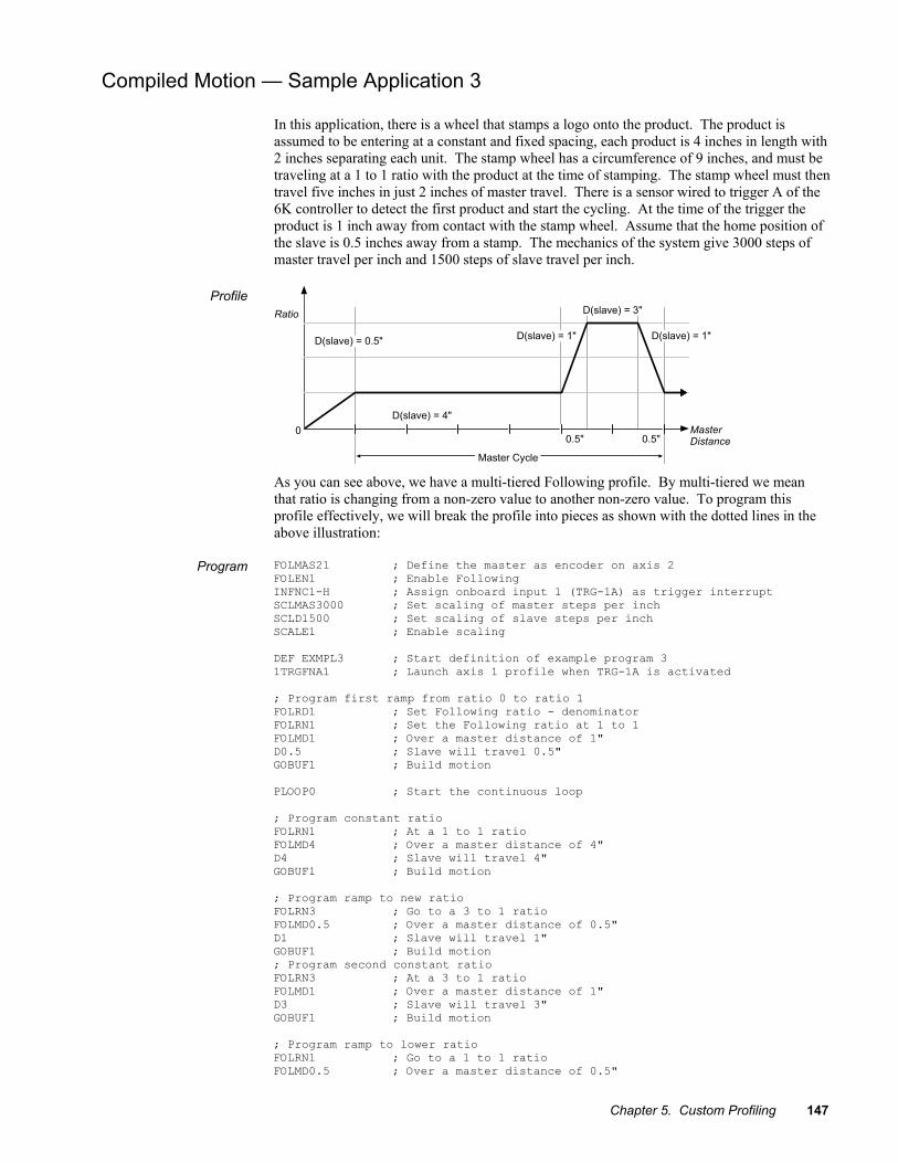
Chapter 5. Custom Profiling 147
Compiled Motion — Sample Application 3
In this application, there is a wheel that stamps a logo onto the product. The product is assumed to be entering at a constant and fixed spacing, each product is 4 inches in length with 2 inches separating each unit. The stamp wheel has a circumference of 9 inches, and must be traveling at a 1 to 1 ratio with the product at the time of stamping. The stamp wheel must then travel five inches in just 2 inches of master travel. There is a sensor wired to trigger A of the 6K controller to detect the first product and start the cycling. At the time of the trigger the product is 1 inch away from contact with the stamp wheel. Assume that the home position of the slave is 0.5 inches away from a stamp. The mechanics of the system give 3000 steps of master travel per inch and 1500 steps of slave travel per inch.
Profile �(�-)
�(���'�-��(�+�
<<�8N
,���(���I�;N
,���(���I�<�8N,���(���I��N
,���(���I�EN
,���(���I��N
<�8N
���������� As you can see above, we have a multi-tiered Following profile. By multi-tiered we mean that ratio is changing from a non-zero value to another non-zero value. To program this profile effectively, we will break the profile into pieces as shown with the dotted lines in the above illustration:
Program FOLMAS21 ; Define the master as encoder on axis 2 FOLEN1 ; Enable Following INFNC1-H ; Assign onboard input 1 (TRG-1A) as trigger interrupt SCLMAS3000 ; Set scaling of master steps per inch SCLD1500 ; Set scaling of slave steps per inch SCALE1 ; Enable scaling DEF EXMPL3 ; Start definition of example program 3 1TRGFNA1 ; Launch axis 1 profile when TRG-1A is activated ; Program first ramp from ratio 0 to ratio 1 FOLRD1 ; Set Following ratio - denominator FOLRN1 ; Set the Following ratio at 1 to 1 FOLMD1 ; Over a master distance of 1" D0.5 ; Slave will travel 0.5" GOBUF1 ; Build motion PLOOP0 ; Start the continuous loop ; Program constant ratio FOLRN1 ; At a 1 to 1 ratio FOLMD4 ; Over a master distance of 4" D4 ; Slave will travel 4" GOBUF1 ; Build motion ; Program ramp to new ratio FOLRN3 ; Go to a 3 to 1 ratio FOLMD0.5 ; Over a master distance of 0.5" D1 ; Slave will travel 1" GOBUF1 ; Build motion ; Program second constant ratio FOLRN3 ; At a 3 to 1 ratio FOLMD1 ; Over a master distance of 1" D3 ; Slave will travel 3" GOBUF1 ; Build motion ; Program ramp to lower ratio FOLRN1 ; Go to a 1 to 1 ratio FOLMD0.5 ; Over a master distance of 0.5"

148 6K Series Programmer’s Guide
D1 ; Slave will travel 1" GOBUF1 ; Build motion PLN1 ; Close motion loop ; Define the exit motion FOLRN0 ; Stop slave at zero ratio (and zero velocity) FOLMD1 ; Over a master distance of 1" D0.5 ; And a slave distance of 0.5" GOBUF1 ; Build motion END ; End definition of example program 3 PCOMP EXMPL3 ; Compile example program 3 ; ********************************************************** ; * To execute the program, enter the PRUN EXMPL3 command * ; **********************************************************
NOTE: The GOBUF command has been added to the “Define the exit motion” portion of the program despite the fact that an infinite loop has been programmed earlier in the program. This is to avoid an error message when the program is compiled.
Compiled Motion — Sample Application 4 A manufacturer of stamped molds needs to make a machine that will stamp molds into a continuous flow of extruded plastic material. The stamp must be lowered 0.5 inches into the plastic to leave the correct impression. Because the flow is continuous, the stamp must also move in synchronization with plastic in the direction of flow as it is lowered and raised. The initial design approach to the machine required two axes of motion. One was needed to lower and raise the stamp, the other to allow the stamp to follow the plastic. With the availability of complex Following cam profiles the job can done with a single axis.
In the drawing below, the stamp is attached to a rotating arm in such a way that the stamp remains level as the arm rotates. The length of the arm at the stamp fixture, or radius of rotation, is exactly one inch. The arm is mounted above the plastic so that at the bottom of its rotation (270 degrees), the stamp will be 0.5 inches into the plastic. Using trigonometry, the horizontal and vertical positions and speeds can be calculated at other arm angles. Because the stamp must follow the flow of the plastic, we must adjust the ratio of rotational speed to plastic speed so that the horizontal velocity component of the arm stays at 1:1 with the plastic while the stamp is in the plastic.
0 0
E<H
0
E<H
The table below shows these relationships. The arm is directly driven with a servo motor having 4096 steps per revolution. The table shows increments of 30 degrees, which is about 341 servo motor steps, or about 0.524 slave inches measured around the circumference described by rotation of the arm. The plastic flow is measured with an encoder giving 1000 steps per inch of flow. To maintain ratios in terms of inches, FOLRD will always be 1000. The required FOLRN value is simply the inverse of the arm’s horizontal velocity component multiplied by the number of slave steps per inch. The corresponding ratio in terms of surface speeds is given in parentheses. The required FOLMD is the number of master steps corresponding to the horizontal component of slave rotation.

Chapter 5. Custom Profiling 149
Arm angle, degrees
Horizontal component (in.) = cos(deg)
FOLMD = 1000 * delta cos(deg)
Horizontal vel component = -sin(deg)
Required FOLRN = -651.9/sin(deg)
210 -0.866 n/a 0.500 1304 (2:1) 240 -0.500 366 0.866 753 (1.155:1) 270 0.000 500 1.000 652 (1:1) 300 0.500 500 0.866 753 (1.155:1) 330 0.866 366 0.500 1304 (2:1)
The profile that we construct from these number is meant to approximate the inverse sine function in the last column, but of course, will actually be a series of ramps and constant ratio segments. Let’s review the Compiled Following Move Distance Calculations to determines the exact shape and error in the first motion segment( from 210 to 240 degrees). First, we need to determine if the ramp or constant ratio is first for that segment. Using ratios and distances in inches, we have:
R1 = 2......................................... Starting ratio R2 = 1.155.................................. Final ratio D = (2*pi)/12 = 0.524 .................. Distance at stamp hinge FOLMD=.366.............................. Travel along plastic
We find (R1+R2) * FOLMD/2 = 0.577, which is greater than D, so the “Ramp First” equations apply to this segment. Let’s examine the error at the junction between the ramp and constant ratio portion of this segment.
MD1 = [D - (R2 * FOLMD)] / ( (R1 - R2) / 2) = 0.239 master inches D1 = 0.5 * (R1 + R2) * MD1 = 0.377 slave inches at circumference = 21.6 degrees cos(210+21.6) - cos(210) = -0.621 - (-0.866) = 0.245 inches slave horizontal travel error = horizontal slave travel - master travel = 0.245 - 0.239 = 0.006 inches
A similar calculation can be done for the “elbow” of the next of the next segment, and symmetry indicates these errors will be the same between 270 and 330 degrees. The error along intermediate points can be found with linear interpolation of ratio and master distance. In this case, the errors fall within manufacturing tolerance. If the errors were too large, the travel could be broken into more segments, each with exactly correct positions and ratios at their boundaries.
So far, we have only discussed the portion of the profile that lowers and raises the stamp. During the remainder of the profile, the arm must continue its rotation to bring the stamp to its starting position in time for the next mold. The mold is 3 inches long, and .4 inches are needed between molds for strength at the edges. This makes the total master cycle 3.4 inches long. The total slave cycle must be 4096 steps, so the segments required to bring the arm around must complete the portions of master and slave cycles not already accounted for. We will create two segments, which divide the remaining master and slave travels in two, and are mirror images of each other. The average ratio of these two segments must simply be slave travel divided by master travel, i.e., (D / FOLMD). As previously determined, the FOLRN value for the boundaries of the stamping portion of the profile is 638. From this value and the average ratio, we can calculate the peak FOLRN value.
D = 0.5 * remaining slave = 0.5 * (4096 - 4 * 341) = 1366 FOLMD = 0.5 * remaining master = 0.5 * [1000 * (3.4 - 2 * 0.866)] = 834 peak ratio = FOLRN/1000 0.5 * (FOLRN/1000 + 1304/1000) = average ratio = D / FOLMD = 1366 / 834 = 1.638 FOLRN = 1972 (solved from above)
Finally, we need to design a segment used to create a smooth entry into the repetitive portion of the profile. We’ll assume that the home position of the arm is at 180 degrees, so it needs to achieve the FOLRN ratio of 1304 in 30 degrees (341 slave steps). Using the same averaging arithmetic as above, the required master distance for the entry segment is 523 steps. A sensor is positioned with this entry segment in mind, and wired to TRG-1A. A function to start motion when the sensor is triggered will be imbedded inside the profile. The motion segments for the stamping portion and recovery portions of the profile must be enclosed in a loop, and can be programmed by picking the numbers from the table and equations above. Because the ratio denominators are the same for all segments, and the slave distances are the same for the entry and each of the stamping segments, these are commanded only when the values change.

150 6K Series Programmer’s Guide
Repetitive Portion of Profile �� ��
�(���'%�'(3�/
8:
�8E
�E<;
�=�:
�<<< �E �F :E :�E: E8 ;;<<
������ ��������
-�������� �����E;����(�������
*��(����������
Program FOLMAS21 ; Follow extra encoder FOLEN1 ; Enable Following mode INFNC1-H ; Enable trigger 1 (TRG-1A) for interrupt function SCALE0 ; Parameters are in steps
DEF STAMP ; Start program definition 1TRGFNA1 ; Axis 1 profile starts upon trigger 1 (TRG-1A) FOLRD1000 ; Ratio denominator, 1ØØØ steps per inch ;define the entry segment D341 ; Distance of 341 steps is about 3Ø degrees FOLRN13Ø4 ; Goal ratio for start segment FOLMD523 ; Master distance during ramp GOBUF1 ; Build start segment PLOOP0 ; Start the continuous loop ;this profile section starts 2-to-1 ratio, or a starting FOLRN13Ø4 FOLRN753 ; Goal ratio for segment FOLMD366 ; Master travel in steps for segment GOBUF1 ; Build motion segment ;the 2nd section of profile starts with the final ratio of the 1st section FOLRN652 ; Goal ratio for segment FOLMD500 ; Master travel in steps for segment GOBUF1 ; Build motion segment ;the next two sections are mirror images of the first two FOLRN753 ; Goal ratio for third segment FOLMD500 ; Master travel in steps for 3rd segment GOBUF1 ; Build motion segment FOLRN1304 ; Goal ratio for 4th segment FOLMD366 ; Master travel in steps for 4th segment GOBUF1 ; Build motion segment ;the next two sections complete the loop and are mirror images of each other D1366 ; Slave travel in recovery segments FOLMD834 ; Master travel in steps for recovery segments FOLRN1972 ; Goal ratio for ramp up segment GOBUF1 ; Build ramp up motion segment FOLRN523 ; Goal ratio for ramp down segment GOBUF1 ; Build ramp down motion segment PLN1 ; End of loop cycle ;finally, a segment to end motion D341 ; Distance of 341 steps is about 3Ø degrees FOLRN0 ; Goal ratio for end segment FOLMD1000 ; Master distance during ramp GOBUF1 ; Build end segment END ; End of STAMP program definition
PCOMP STAMP ; Compile the program
; ********************************************************** ; * To execute the program, enter the PRUN STAMP command * ; **********************************************************

Chapter 5. Custom Profiling 151
On-the-Fly Motion (pre-emptive GOs) While motion is in progress, you can change these motion parameters to affect a new profile:
• Acceleration (A) — s-curve acceleration is not allowed • Deceleration (AD) — s-curve deceleration is not allowed • Velocity (V) • Distance (D) • Preset or Continuous Positioning Mode Selection (MC) • Incremental or Absolute Positioning Mode Selection (MA) • Following Ratio Numerator and Denominator (FOLRN and FOLRD, respectively)
The motion parameters can be changed by sending the respective command (e.g., A, V, D, MC) followed by the GO command. If the continuous command execution mode is enabled (COMEXC1), you can execute buffered commands; otherwise (COMEXCØ), you must prefix each command with an immediate command identifier (e.g., !A, !V, !D, !MC, followed by !GO).
The new GO command pre-empts the motion profile in progress with a new profile based on the new motion parameter(s). On-the-fly motion changes are applicable only for motion started with the GO command, and not for motion started with other commands such as HOM, JOG, JOY, PRUN or GOL.
On-the-fly motion changes are most likely to be used to change the velocity and/or goal position of a preset move already underway. In the event that the goal position is completely unknown before motion starts, a move can be started in continuous mode (MC1), with a switch to preset mode (MCØ), a distance command (D), and a GO given later. In absolute positioning mode (MA1) the new goal position given with a pre-emptive GO is explicit in the D command. In incremental positioning (MAØ) the distance given with a new pre-emptive GO is always measured from the at-rest position before the original GO. If a move is stopped (with the S command), and then resumed (with the C command), this resumed motion is considered to be part of the original GO. A subsequent distance given with a new pre-emptive GO is measured from the at rest position before the original GO, not the intermediate stopped position.
Programming Example: This program creates a 2-tiered profile (single-axis) that changes velocity and deceleration at specific motor positions.
SCALE0 ; Disable scaling DEL OTF ; Delete program (in case program is already in memory) DEF OTF ; Begin definition of program PSET0 ; Set position to zero COMEXC1 ; Enable continuous command processing mode MC0 ; Select preset positioning MA0 ; Select incremental positioning A20 ; Set accel to 20 revs/sec/sec AD20 ; Set decel to 20 revs/sec/sec V9 ; Set velocity to 9 revs/sec D500000 ; Set distance to 20 revs GO1 ; Initiate motion WAIT(PC>100000) ; Wait until commanded position > 100000 steps (4 revs) V4 ; Slow down for machine operation GO1 ; Initiate new profile with new velocity WAIT(PC>450000) ; Wait until the motor position > 450000 steps (18 revs) AD5 ; Set decel for gentle stop V1 ; Slow down for gentle stop GO1 ; Initiate new profile with new velocity END ; End program definition

152 6K Series Programmer’s Guide
The table below summarizes the restrictions on pre-emptive GOs.
Condition Possible?
Execute GO during MC1 & FOLENØ Yes
Execute GO during MC1 & FOLEN1 Yes
Execute GO during MCØ & FOLENØ Yes
Execute GO during MCØ & FOLEN1 No
Change MC setting during motion Yes (but cannot change MC1 to MCØ during FOLEN1)
Change ENC setting during motion No
Change FOLENØ to FOLEN1 during motion No
Change FOLEN1 to FOLENØ during motion Only while MC1, constant ratio, and not shifting
OTF Error Conditions The ability to change the goal position on the fly raises the possibility of several error conditions:
6K Response Error Conditions
Set axis status bit 30
Set error status bit 10
Kill motion (decelerate at the LHAD value)
The new position goal of an on-the-fly GO cannot be reached with the current direction, velocity, and decel.
YES
YES
NO
The direction of the new goal position is opposite that of current travel
YES
YES
YES
Further instructions about handling error conditions are provided on page 30.
There has not yet been an overshoot, but it is not possible to decelerate to the new distance from the current velocity using the specified AD value.
YES
YES
YES
RELATED STATUS COMMANDS
Axis Status — Bit 30: (this status bit is cleared with the next GO command) AS.30 ....Assignment & comparison operator — use in a conditional expression (see page 25). TASF ......Full text description of each status bit. (see “Preset Move Overshot” line item) TAS ........Binary report of each status bit (bits 1-32 from left to right). See bit 30.
Error Status — Bit 10: The error status is monitored and reported only if you enable error-checking bit 10 with the ERROR command (e.g., ERROR.1Ø-1). NOTE: When the error occurs, the controller with branch to the error program (assigned with the ERRORP command). (this status bit is cleared with the next GO command) ER.10 ....Assignment & comparison operator — use in a conditional expression (see page 25). TERF ......Full text description of each status bit. (see “Preset Move Overshot” line item) TER ........Binary report of each status bit (bits 1-32 from left to right). See bit 10.
Scenarios
Scenario 1: OTF change of velocity and distance, where new commanded distance (D2) is greater than the original distance (D1) that was pre-empted [D2 >D1]. The distances are the areas under the profiles, starting at t0 for both. If the original move had continued, D1 would have been reached at time t1. D2 is reached at time t2.
(
�
,�
,:
�� �:�<

Chapter 5. Custom Profiling 153
Scenario 2: OTF change of distance, where new commanded distance (D2) is less than the original distance (D1) that was pre-empted [D2 < D1]. In this example, the position where the OTF change was entered is already beyond D2 (or D2 cannot be reached with the commanded deceleration). The result is an error and motion is killed (decel at the LHAD value) and TAS bit 30 and TER bit 10 are set.
(
�
,�,:
���<
Scenario 3: OTF change of velocity. Note that motion must continue for a longer time at the reduced velocity to reach the original commanded distance than if it had continued at the original velocity (t2 > t1).
(
�
,�
�� �:�<
,�
On-The-Fly Motion — Sample Application A manufacturer of three products wishes to produce a “sampler-pak” package that will contain a few of each of his products. The products all have the same width and length, but are 3, 4, and 5 inches high respectively. The 3 products are fed from individual lines into a common conveyor, and arrive at a stacking and wrapping station. At this station, a tray accepts a product and must have moved down by that product’s height by the time the next product arrives. This means that each time a new product arrives, the velocity of the tray must be changed to match the height of that product. Although product spacing will be regular, the ordering of product type on the common conveyor will be random, due to variations in the input lines. Also, a finished sampler-pak should contain 5 products or be at least 18 inches high, whichever occurs first. This means that the total move distance of the tray will be unknown until the last product arrives. When the last product is stacked, an output is asserted that will pause the conveyor and start the wrapping process. When wrapping is complete, the sampler-pak is removed from the tray, and the tray returns to the starting position.
The basic problems in this application are that the move distance is not known until near the end, and the velocity must change on the fly. As the products approach the tray, they are detected with a near vertical arrangement of three sensors. Products of heights 3, 4, and 5 inches are detected by 1, 2, or all 3 sensors respectively. Input 1 always detects a product, and switches last, so that the others will be stable. When each product is identified, the motion profile is modified accordingly.

154 6K Series Programmer’s Guide
�� ����
EN ;N ;N 8N 8NEN ;N�
:E
EN
EN
Program (portion only)
VAR1=0 ; Initialize product count VAR2=0 ; Initialize move distance variable VAR3=0 ; Initialize velocity A10 ; Moderate acceleration MC0 ; Start with preset move WHILE(VAR1<5 AND VAR2<18) ; Loop until cycle complete WAIT(IN.1=B1) ; Wait for start of next product ; (onboard input 1 is activated) VAR1=VAR1+1 ; Update product count IF(IN.2=B1) ; If not a 3" product IF(IN.3=B1) ; If it is a 5" product VAR3=5 ; Set velocity VAR2=VAR2+5 ; Update distance ELSE ; If not 5", must be 4" VAR3=4 ; Set velocity VAR2=VAR2+4 ; Update distance NIF ; End of 5" case check ELSE ; 3" inch case VAR3=3 ; Set velocity VAR2=VAR2+3 ; Update distance NIF ; End of 3" case check V(VAR3) ; New velocity D(VAR2) ; New distance WAIT(IN.1=B0) ; Wait for end of this product GO1 ; Implement new distance and velocity NWHILE ; Sampler-pak completed product detection WAIT(AS.1=B0) ; Wait for move to complete OUT1 ; Output to indicate stacking complete

Chapter 5. Custom Profiling 155
Registration A “registration input” is
a trigger input assigned the “trigger interrupt”
function with the INFNCi-H command.
When a registration input is activated, the motion profile currently being executed is replaced by the registration profile with its own distance (REG), acceleration (A & AA), deceleration (AD & ADA), and velocity (V) values. The registration move can interrupt any preset, continuous, or registration move in progress.
The registration move does not alter the rest of the program being executed when registration occurs, nor does it affect commands being executed in the background if the controller is operating in the continuous command execution mode (COMEXC1).
Registration moves will not be executed while the motor is not performing a move, while in the joystick mode (JOY1), or while decelerating due to a stop, kill, soft limit, or hard limit.
How to Set up a Registration Move
ENCCNT: Encoder
capture options for stepper axis are
discussed on page 66.
Before you can initiate a registration move, you must program these elements (refer also to the programming examples below):
1. Configure one of the trigger inputs (TRG-nA or TRG-nB per axis) to function as a trigger interrupt input; this is done with the INFNCi-H command, where “i” is the input bit number representing the targeted trigger input. Note that the “Master Trigger” input cannot be used for registration.
2. Specify the distance of the registration move with the REG command. For servo axes, the distance refers to the encoder position (registration cannot be used with analog input feedback). For stepper axes, the distance refers to commanded position if ENCCNT0 (default setting) or encoder position if ENCCNT1.
3. Enable the registration function with the RE command. Registration is performed only on the axis or axes with the registration function enabled, and with a non-zero distance specified in the respective axis-designation field of the REG command; the other axes will not be affected. Each trigger has a distinct move defined for its axis; for example, trigger 3 (called TRG-2A) can initiate a registration move for axis 2 with the specified 2REGA distance.
NOTE: The registration move is executed using the A, AA, AD, ADA, and V values that were in effect when the REG command was entered.
Registration Move Accuracy(see also Registration Move Status below) The accuracy of the registration move distance specified with the REG command is ±1 count (servo axes: encoder count; stepper axes: commanded count if ENCCNT0 or encoder count if ENCCNT1).
RULE OF THUMB: To prevent position overshoot, make sure the REG distance is greater than 4 ms multiplied by the incoming velocity.
The lapse between activating the registration input and commencing the registration move (this does not affect the move accuracy) is less than one position sample period (2 ms).
The REG distance will be scaled by the distance scale factor (SCLD value) if scaling is enabled (SCALE1). See page 51 for details on scaling.
156 6K Series Programmer’s Guide
Preventing Unwanted Registration Moves (methods) • Registration Input Debounce: Registration Input Debounce: By default, the registration
inputs are debounced for 2 ms before another input on the same trigger is recognized. (The debounce time is the time required between a trigger's initial active transition and its secondary active transition.) Therefore, the maximum rate that a registration input can initiate registration moves is 500 times per second. If your application requires a shorter debounce time, you can change it with the TRGLOT command.
• Registration Single-Shot: The REGSS command allows you to program the 6K controller to ignore any registration commands after the first registration move has been initiated. Refer to the REGSS command description for further details and an application example.
• Registration Lockout Distance: The REGLOD command specifies what distance an axis must travel before any trigger assigned as a registration input will be recognized. Refer to the Sample Application 3 below.
Registration Move Status & Error Handling Axis Status — Bit 28: This status bit is set when a registration move has been initiated by any registration input (trigger). This status bit is cleared with the next GO command.
AS.28 .......Assignment & comparison operator — use in a conditional expression (see page 25). TASF..........Full text description of each status bit. (see “Reg Move Commanded” line item) TAS ............Binary report of each status bit (bits 1-32 from left to right). See bit 28.
Axis Status — Bit 30: If, when the registration input is activated, the registration move profile cannot be performed with the specified motion parameters, the 6K controller will kill the move in progress and set axis status bit 30. This status bit is cleared with the next GO command.
AS.3Ø .......Assignment & comparison operator — use in a conditional expression (see page 25). TASF..........Full text description of each status bit. (see “Preset Move Overshot” line item) TAS ............Binary report of each status bit (bits 1-32 from left to right). See bit 30.
Further instructions about handling error conditions are provided on page 30.
Error Status — Bit 10: This status bit can be set if axis status bit 30 is set. The error status is monitored and reported only if you enable error-checking bit 10 with the ERROR command (e.g., ERROR.1Ø-1). NOTE: When the error occurs, the controller will branch to the error program (assigned with the ERRORP command). This status bit is cleared with the next GO command.
ER.1Ø .......Assignment & comparison operator — use in a conditional expression (see page 25). TERF..........Full text description of each status bit. (see “Preset Move Overshot” line item) TER ............Binary report of each status bit (bits 1-32 from left to right). See bit 10.
Trigger Status — Bits 1-17: Trigger status bits are set when a registration move has been initiated by trigger inputs A or B for each axis, or with the TRIG-M (master trigger) input. This also indicates that the positions of all axes has been captured. As soon as the captured information is transferred or assigned/compared (see page 84), the respective trigger status bit is cleared (set to Ø).
TRIG..........Assignment & comparison operator — use in a conditional expression.(see page 25). TTRIG .......Binary report of each status bit (bits 1-17 from left to right). From left to right the bits
represent trigger A and B for axes 1-8, the 17th bit is master trigger M (the “MASTER TRIG” input terminal) — see page 76.

Chapter 5. Custom Profiling 157
Registration — Sample Application 1 In this example, two-tiered registration is achieved (see illustration below). While axes 1 is executing it’s 50,000-unit move, trigger input 1 (TRG-1A) is activated and executes registration move A to slow the load's movement. An open container of volatile liquid is then placed on the conveyor belts. After picking up the liquid and while registration move A is still in progress, trigger input 2 (TRG-1B) is activated and executes registration move B to slow the load to gentle stop.
DEL REGI1 ; Delete program (in case program already resides in memory) DEF REGI1 ; Begin program definition INFNC1-H ; Define trigger input 1 (TRG-1A) as trigger interrupt input INFNC2-H ; Define trigger input 2 (TRG-1B) as trigger interrupt input A20 ; Set acceleration on axis 1 to 20 units/sec2 AD40 ; Set deceleration on axis 1 to 40 units/sec2 V1 ; Set velocity on axis 1 to 1 unit/sec 1REGA4000 ; Set TRG-1A's registration distance on axis 1 to 4000 units ; (registration A move will use the A, AD, & V values above) A5 ; Set acceleration on axis 1 to 5 units/sec/sec AD2 ; Set deceleration on axis 1 to 2 units/sec/sec V.5 ; Set velocity on axis 1 to 0.5 units/sec 1REGB13000 ; Set TRG-1B's registration distance on axis 1 to 13,000 units ; (registration B move will use the A, AD, & V values above) RE10 ; Enable registration on axis 1 only A50 ; Set acceleration to 50 units/sec/sec on axis 1 AD50 ; Set deceleration to 50 units/sec/sec on axis 1 V10 ; Set velocity to 10 unit/sec on axis 1 D50000 ; Set distance to 50000 units on axis 1 GO10 ; Initiate motion on axis 1 END ; End program definition
v
D0
1st Registration mark(TRG-1A) occurs
2nd Registration mark(TRG-1B) occurs
2
4
6
8
10
20,00010,0000
Pick upcontainer
here

158 6K Series Programmer’s Guide
Registration — Sample Application 2 A user has a line of material with randomly spaced registration marks. It is known that the first mark must initiate a registration move, and that each registration move cannot be interrupted or the end product will be destroyed. Since the distance between marks is random, it is impossible to predict if a second registration mark will occur before the first registration move has finished. DEL REGI2 ; Delete program (in case program already resides in memory) DEF REGI2 ; Begin program definition INFNC1-H ; Trigger capture mode for trigger 1 (TRG-1A) RE1 ; Enable registration V2 ; Set registration move to a velocity of 2 rps AD.5 ; a deceleration of 0.5 rev/sec/sec 1REGA20000 ; and a distance of 20000 steps for axis 1 MC1 ; Start a mode continuous V1 ; move at a velocity of 1 rps GO1 ; Initiate motion END ; End program definition
v
t0
1
2
1st Registrationmark occurs
2nd Registrationmark occurs The first registration move
is pre-empted by a secondregistration input.
In order to stop the second registration from occurring, REGSS can be used:
DEL REGI2b ; Delete program (in case program already resides in memory) DEF REGI2b ; Begin program definition INFNC1-H ; Trigger capture mode for trigger 1 (TRG-1A) RE1 ; Enable registration V2 ; Set registration move to a velocity of 2 rps 1REGA20000 ; and a distance of 20000 steps for axis 1 REGSS1 ; Enable registration single shot mode MC1 ; Start a mode continuous V1 ; move at a velocity of 1 rps GO1 ; Initiate motion END ; End program definition
v
t0
1
2
1st Registrationmark occurs
2nd Registrationmark occurs Because of REGSS, the
first registration move isNOT pre-empted by thesecond registration input.The registration “singleshot” will be reset whenyou issue a new motioncommand (GO, PRUN, etc.).

Chapter 5. Custom Profiling 159
Registration — Sample Application 3 A print wheel uses registration to initiate each print cycle. From the beginning of motion, the controller should ignore all registration marks before traveling 2000 steps. This is to ensure that the unit is up to speed and that the registration mark is a valid one. DEL REGI3 ; Delete program (in case program already resides in memory) DEF REGI3 ; Begin program definition INFNC1-H ; Trigger capture mode for trigger 1 (TRG-1A)) RE1 ; Enable registration V2 ; Set registration move to a velocity of 2 rps 1REGA2500 ; and a distance of 2500 steps for axis 1 REGLOD2000 ; Set registration lockout distance to 2000 steps MC1 ; Start a mode continuous V1 ; move at a velocity of 1 rps GO1 ; Initiate motion END ; End program definition
v
t0
1
2
1st Registration mark occursafter 1500 steps, but theregistrationmove does notoccur becausethe lockoutdistance is setto 2000 steps.
2nd Registrationmark occurs after3000 steps.
Synchronizing Motion (GOWHEN and TRGFN operations) GOWHEN and TRGFN allow you to synchronize the execution of motion on one or more axes:
• GOWHEN — synchronize execution of the subsequent start-motion command (GO, GOL, FGADV, FSHFC, or FSHFD) to: - Position (commanded, feedback device, motor, master, slave, Following shift) - Master cycle number - Input status - Time delay (dwell)
• TRGFN: - Suspend execution of the next start-motion command (GO, GOL, FGADV, FSHFC, or FSHFD) until the specified trigger input goes active. - Suspend beginning a new Following master cycle until the specified trigger input goes active.
Conditional “GO”s (GOWHEN) The GOWHEN command is used to synchronize a motion profile of an axis with a specified position count, input status, dwell (time delay), or master cycle number on that axis or other axes. Command processing does not wait for the GOWHEN conditions (relational expressions) to become true during the GOWHEN command. Rather, the motion from the subsequent start-motion command (GO, GOL, FGADV, FSHFC, and FSHFD) will be suspended until the condition becomes true.
Start-motion type commands that cannot be synchronized using the GOWHEN command are: HOM, JOG, JOY, and PRUN. A preset GO command that is already in motion can start a new profile using the GOWHEN and GO sequence of commands. Continuous moves (MC1) already in progress can change to a new velocity based upon the GOWHEN and GO sequence. Both preset and continuous moves can be started from rest with the GOWHEN and GO sequence.

160 6K Series Programmer’s Guide
GOWHEN Syntax ����#����� ����$��� ����$��� ����$��%�%�%
*����� ��-5������� ��� ��5"
!5���� !5���: !5���E
�������������������������������������������������
��������2��������"
&'������� 6�����&���(���������� ������� .�����������������������'�������� �����,��(������� ����� ����������� �#������� - ������������ �)�*����������������� �*+(��� ��(��������� �*�&��� 6��'� ���������������� # ������������������� ,'���� ������� ���
��������2��������"
�������
��������2��������"
G +������(���������� ���������
G ,������ ��� �G 7� ����(�����!"""������������� �� ������������� �
��������
����#��,�#�-....� /� 0 ����������0������� �,��1������ ��������-....����#����%2�!,� /� 0 ����������0�������!��������0��32�� ��1��4�����!,�����#��5�)�*�566� /� 0 ����������0��������7� ��������� �5���
/����4���566�7� ����� ���1�0���
SCALING
If scaling is enabled (SCALE1), the right-hand operand is multiplied by SCLD if the left-hand operand is FB, PC, PE, PSLV, or PSHF. The right-hand operand is multiplied by the SCLMAS value if the left-hand operand is PMAS. (The SCLD or SCLMAS values used correlate to the axis specified with the variable–e.g., a GOWHEN expression with 3PE scales the encoder position by the SCLD value specified for axis 3.)
GOWHEN Status
Axis Status — Bit 26: Bit 26 is set when motion has been commanded by a GO, GOL, FGADV, FSHFC, or FSHFD command, but is suspended due to a pending GOWHEN condition. This status bit is cleared when the GOWHEN condition is true or when a stop (!S) or kill (!K or ^K) command is executed. An individual axis' GOWHEN command can be cleared using an axis-specific S or K command (e.g., !S11XØ or !KØXX1).
AS.26 .......Assignment & comparison operator — use in a conditional expression (see page 25). TASF..........Full text description of each status bit. (see “Gowhen is Pending” line item) TAS ............Binary report of each status bit (bits 1-32 from left to right). See bit 26.
Axis Status — Bit 29: Bit 29 is set when the input state of position relationship specificed in the GOWHEN expression was already true when the subsequent GO, GOL, FGADV, FSHFC or FSHFD command was executed. AS.29 .......Assignment & comparison operator — use in a conditional expression (see page 25). TASF..........Full text description of each status bit. (see “Gowhen Error” line item) TAS ............Binary report of each status bit (bits 1-32 from left to right). See bit 29.

Chapter 5. Custom Profiling 161
Further instructions about handling error conditions are provided on page 30.
Error Status — Bit 14: Bit 14 is set if the input state or position relationship specified in the GOWHEN expression was already true when the subsequent GO, GOL, FGADV, FSHFC, or FSHFD command is issued. The error status is monitored and reported only if you enable error-checking bit 14 with the ERROR command (e.g., ERROR.14-1). NOTE: When the error occurs, the controller with branch to the error program (assigned with the ERRORP command).
ER.14 .......Assignment & comparison operator — use in a conditional expression (see page 25). TERF..........Full text description of each status bit. (see “GOWHEN condition true” line item) TER ............Binary report of each status bit (bits 1-32 from left to right). See bit 14.
GOWHEN ... On a Trigger Input
If you wish motion to be triggered with a trigger input, use the aTRGFNc1 command. The aTRGFNc1 command executes in the same manner as the GOWHEN command, except that motion is executed on specified axis “a” when the specified trigger input “c” is activated. For more information, see Trigger Functions below.
GOWHEN vs.WAIT A WAIT will cause the 6K controller program to halt program flow (except for execution of immediate commands) until the condition specified is satisfied. Common uses for this function include delaying subsequent I/O activation until the master has achieved a required position or an object has been sensed.
By contrast, a GOWHEN will suspend the motion profile for a specific axis until the specified condition is met. It does not affect program flow. If you wish motion to be triggered with a trigger input, use the TRGFNc1 command. The TRGFNc1 command executes in the same manner as the GOWHEN command, except that motion is executed when the specified trigger input (c) is activated (see Trigger Functions below for details). In addition, GOWHEN expressions are limited to the operands listed above; WAIT can use additional operands such as FS (Following status) and VMAS (velocity of master).
Factors Affecting GOWHEN Execution
If, on the same axis, a second GOWHEN command is executed before a start-motion command (GO, GOL, FSHFC, or FSHFD), then the first GOWHEN is over-written by the second GOWHEN command. (GOWHEN commands are not nested.) An error is not generated when a GOWHEN command is over-written by another GOWHEN.
While waiting for a GOWHEN condition to be met and a start-motion command has been issued, if a second GOWHEN command is encountered, then the first sequence is disabled and another start-motion command is needed to re-arm the second GOWHEN sequence.
A new GOWHEN command must be issued for each start-motion command (GO, GOL, FGADV, FSHFC, or FSHFD). That is, once a GOWHEN condition is met and the motion command is executed, subsequent motion commands will not be affected by the same GOWHEN command.
If the GOWHEN and start-motion commands are issued, the motion profile is delayed until the GOWHEN condition is met. If a second start-motion command is encountered, the second start-motion command will override the GOWHEN command and start motion. If this override situation is not desired, it can be avoided by using a WAIT condition between the first start-motion command and the second start-motion command.
It is probable that the GOWHEN command, the GO command, and the GOWHEN condition becoming true can be separated in time, and by other commands. Situations can arise, or commands can be given that make the GOWHEN invalid or inappropriate. In these cases, the GOWHEN condition is cleared, and any motion pending the GOWHEN condition becoming true is canceled. These situations include execution of the JOG, JOY, HOM, PRUN, and DRIVEØ commands, as well motion being stopped due to hard or soft limits, a drive fault, an immediate stop (!S), or an immediate kill (!K or ^K).

162 6K Series Programmer’s Guide
GOWHEN in Compiled
Motion (Compiled Motion is discussed on
page 136)
When used in a compiled program, a GOWHEN will pause the profile in progress (motion continues at constant velocity) until the GOWHEN condition evaluates true. When executing a compiled Following profile, the GOWHEN is ignored on the reverse Following path (i.e., when the master is moving in the opposite direction of that which is specified in the FOLMAS command). A compiled GOWHEN can require up to 4 segments of compiled memory storage.
Sample 6K Code
In the example below, axis 2 must start motion when the actual position of axis 1 has reached 4. While axis 1 is moving, the program must be monitoring inputs and serving other system requirements, so a WAIT statement cannot be used; instead, a GOWHEN and GO sequence will delay the profile of axis 2.
MC00 ; Set both axes to preset move mode D20,20 ; Set distance end-point COMEXC1 ; Enable continuous command execution mode V1,1 ; Set velocity A100,100 ; Set acceleration GOWHEN(,1PE>4) ; Delay axis 2 profile. When expression is true (position ; of encoder 1 is > 4), allow axis 2 to start motion. GO11 ; Command both axes to move. Axis 2 will not start until ; conditions in the GOWHEN statement are true. ; Command processing does not wait, so other system ; functions can be performed.
Trigger Functions (TRGFN) The Trigger Functions command (TRGFN) allows you to assign additional functions to trigger inputs that have been defined as “trigger interrupt” inputs (INFNCi-H):
!��������� �"#����������$�������
������
����%�&�'�����!�� ����������$�������
������ ������������(����������������))�����*�����+'����������+�� �����'������� ���,�������
�(������,�
• “Conditional GO” Function (aTRGFNc1x): Suspend execution of the next start-motion command on axis “a” until specified trigger input “c” goes active. Start-motion commands are listed below. Refer to page 159 or to the GOWHEN command description for additional details.
- GO (standard command to begin motion) - GOL (begin linear interpolated motion) - FGADV (begin geared advance – for Following motion) - FSHFC (begin continuous shift – for Following motion) - FSHFD (begin preset shift – for Following motion)
Axis status bit 26 (reported with TASF, TAS, or AS) is set to one (1) when there is a pending “Conditional GO” condition initiated by a TRGFN command; this bit is cleared when the trigger is activated or when a stop command (S) or a kill command (K) is issued. If you need execution to be triggered by other factors (e.g., input state, master position, encoder position, etc.) use the GOWHEN command.

Chapter 5. Custom Profiling 163
• “New Master Cycle” Function (aTRGFNcx1): This is equivalent to executing the FMCNEW command. When specified trigger input “c” goes active, the controller begins a new Following master cycle on axis “a”. For more information on master cycles, see page 183 or to the FMCNEW command description.
These trigger functions are cleared once the function is complete (trigger input is activated). To use the trigger to perform a GOWHEN function again, the TRGFN command must be given again.
Sample 6K Code
INFNC2-H ; Define trigger 2 (TRG-1B) as a trigger interrupt input INFNC4-H ; Define trigger 4 (TRG-2B) as a trigger interrupt input 1TRGFNBx1 ; When TRG-1B goes active, axis 1 will begin a ; new master cycle 2TRGFNB1x ; When TRG-2B goes active, axis 2 will execute the move ; commanded with the GO command. GO01 ; The move on axis 2 is commanded, but will not execute ; until trigger 2B goes active.


6
C H A P T E R S I X
Following
IN THIS CHAPTER This chapter will help you understand Ratio Following:
• Introduction to Ratio Following ......................................................................166 • Implementing Ratio Following .......................................................................168 • Master Cycle Concept .....................................................................................183 • Technical Considerations for Following .........................................................189 • Troubleshooting for Following .......................................................................199 • Following Commands (list).............................................................................200

166 6K Series Programmer’s Guide
Ratio Following – Introduction As part of its standard features, the 6K Series Controller family allows you to solve applications requiring Ratio Following.
Compiled Profiles
You can pre-compile Following profiles (saves processing time). See page 139 for details.
Ratio Following is, essentially, controlled motion based on the measurement of external motion. This includes concepts such as an electronic gearbox, trackball, follower axis feed-to-length, as well as complex changes of ratio as a function of master position. Ratio Following can include continuous, preset, and registration-like moves in which the velocity is replaced with a ratio.
The follower axis can follow in either direction and change ratio while moving, with phase shifts allowed during motion at otherwise constant ratio. Ratio changes or new moves can be dependent on master position or based on receipt of a trigger input. Also, a follower axis can perform Following moves or normal time-based moves in the same application because Following can be enabled and disabled at will. Product cycles (operations that repeat with periodic master travel) can be easily specified with the master cycle concept (see page 183).
In Ratio Following, acceleration ramps between ratios will take place over a user-specified master distance. Product cycles can be easily specified with the master cycle concept.
This chapter highlights the capabilities of the 6K Following features and provides application examples. If you need more details on the operation or syntax of a particular command, please see the 6K Series Command Reference.
Before delving into the specifics of Ratio Following, read on to gain a basic understanding of how the 6K controller follows.
What can be a master? Any axis on the 6K controller can can made to any of the master input (“master”) sources listed in the table below. All of the 6K controller’s axes can be following at the same time with the same or different master.
• Commanded position • Incremental encoder. The encoder can be one of the axis-related “ENCODER” ports, or it
can be the “MASTER ENCODER” port. • Analog input (servo axes only). This requires an ANI SIM be installed on an expansion
I/O brick (see your product’s Installation Guide for instructions). ANI SIMs and expansion I/O bricks are sold separately.
• Internal count source (a “virtual master” option) • Internal sine wave source (a “virtual master” option) • Integer variable (VARI)
A servo axis cannot follow its own feedback device input (encoder or analog input). A stepper axis can follow its own encoder input, as long as that axis does not using the Stall Detect feature (ESTALL1 mode).
For instructions on assigning a master for a particular follower axis, see Define the Master and Follower Axes (page 168), or see the FOLMAS command description in the 6K Series Command Reference.

Chapter 6. Following 167
Following Status (TFSF, TFS & FS Commands)
Many of the Following features described in this document have associated status bits that can be displayed (with the TFSF and TFS commands) or used in assignment or comparison operations (with the FS operator). The portions of this document that describe those features also summarize the related status bits.
FS Bit Function (YES = 1; NO = Ø) 1....... Follower in Ratio Move..... A Following move is in progress. 2....... Ratio is Negative .............. The current ratio is negative (i.e., follower counts counting in the opposite direction from master). 3....... Follower Ratio Changing .. The follower is ramping from one ratio to another (including a ramp to or from zero ratio). 4....... Follower At Ratio .............. The follower is at constant non-zero ratio.
Bits 1-4 indicate the status of the follower axis in Following motion.
* 5....... FOLMAS Active.................. A master is specified with the FOLMAS command. * 6....... FOLEN Active .................... Following has been enabled with the FOLEN command. * 7....... Master is Moving .............. The specified master is currently in motion. 8....... Master Dir Neg ................. The current master direction is negative. (Bit must be cleared to allow Following move in preset
mode—MCØ). Bits 5-8 indicate the status required for Following motion (i.e., a master must be assigned, Following must be enabled, the master must be moving, and for many features, the master direction must be positive). Unless the master is a commanded position of another axis, minor vibration of the master will likely cause bits 7-8 to toggle on and off, even if the master is nominally “at rest”. These bits are meant primarily as a quick diagnosis for the absence of master motion, or master motion in the wrong direction. Many features require positive master counting to work properly.
9....... OK to Shift ........................ Conditions are valid to issue shift commands (FSHFD or FSHFC). 10....... Shifting now...................... A shift move is in progress. 11....... Shift is Continuous............ An FSHFC-based shift move is in progress. 12....... Shift Dir is Neg.................. The direction of the shift move in progress is negative.
Bits 9-12 indicate the shift status of the follower. Shifting is super-imposed motion, but if viewed alone, can have its own status. In other words, bits 10-12 describe only the shifting portion of motion.
13....... Master Cyc Trig Pend....... A master cycle restart is pending the occurrence of the specified trigger. 14....... Mas Cyc Len Given .......... A non-zero master cycle length has been specified with the FMCLEN command. 15....... Master Cyc Pos Neg......... The current master cycle position (PMAS) is negative. This could be by caused by a negative initial
master cycle position (FMCP), or if the master is moving in the negative direction. 16....... Master Cyc Num > 0......... The master position (PMAS) has exceeded the master cycle length (FMCLEN) at least once, causing
the master cycle number (NMCY) to increment.
Bits 13-16 indicate the status of master cycle counting. If a Following application is taking advantage of master cycle counting, these bits provide a quick summary of some important master cycle information.
17....... Mas Pos Prediction On..... Master position prediction has been enabled (FPPEN). 18....... Mas Filtering On ............... A non-zero value for master position filtering (FFILT) is in effect. 19....... <RESERVED> 20....... <RESERVED>
Bit 17 and 18 indicate the status of master position measurement features.
21....... <RESERVED> 22....... <RESERVED> 23....... OK to do FGADV move...... OK to do Geared Advance move (master assigned with FOLMAS, Following enabled with FOLEN, and
follower axis is either not moving, or moving at constant ratio in continuous mode). 24....... FGADV move underway .... Geared Advance move profile is in progress.
Bits 23 and 24 indicate the status of a Geared Advance move.
25....... <RESERVED> 26....... FMAXA/FMAXV limited........ The present Following move profile is being limited by FMAXA or FMAXV. 27....... <RESERVED> 28....... <RESERVED>
Bits 23 and 24 indicate the status of a Geared Advance move.
* All these conditions must be true before Following motion will occur.
168 6K Series Programmer’s Guide
Implementing Ratio Following This section covers the basic elements of implementing Ratio Following:
• Applying Following setup parameters • Move profiles • Performing phase shifts (FSHFC and FSHFD) • Geared advanced (FGADV) • Application scenarios:
- Electronic gearbox - Trackball
Ratio Following Setup Parameters Prior to executing a Following move, there are several setup parameters that must be specified. These parameters can be established:
Programming
examples — see application examples
later in this chapter.
• Define the master and follower axes (FOLMAS) • Define master & follower scaling factors (SCLMAS, SCLA, SCLD, and SCLV) – if required • Define the follower-to-master Following ratio (FOLRN and FOLRD) • Define the master distance (FOLMD) – define scaling first • Enable the Following Mode (FOLEN)
Following Status (see TFSF, TFS and FS commands)
Following Status bits 5-8 (see table below) are meant to indicate the status required for Following motion (i.e., a master must be assigned, Following must be enabled, the master must be moving, and for many features, the master direction must be positive).
Bits 7-8 represent master motion and master direction respectively. Unless the master is a commanded position of another axis, it is likely that minor vibration of the master will cause these bits to toggle on and off, even if the master is nominally “at rest”. These bits are meant primarily as a quick diagnosis for the absence of master motion, or master motion in the wrong direction. Many features require positive master counting to work properly.
Bit No. Function (YES = 1; NO = Ø)
5 FOLMAS Active................A master is specified with the FOLMAS command. 6 FOLEN Active ..................Following has been enabled with the FOLEN command. 7 Master is Moving ............The specified master is currently in motion. 8 Master Dir Neg ...............The current master direction is negative. (bit must be cleared to
allow Following move in preset mode–MCØ).
Define the Master and Follower Axes (FOLMAS)
The FOLMAS command defines the masters and the followers. The command syntax is:

Chapter 6. Following 169
Follower Axis 3
Follower Axis 2
Follower Axis 1
Follower Axis 5
Follower Axis 4
<+ii>
Master source selection
Master source axis # (optional)
Sign Bit
Format for master assignment to follower:
FOLMAS <+ii>,<+ii>,<+ii>,<+ii>,<+ii> ...
• Sign bit (±): Specifies the count direction of the master source that will result in positive master travel counts. The sign bit is not meant to be used simply to change the direction of follower motion. That function can be done with the sign of the D command. Rather, the sign bit is used to allow forward motion of the physical master (e.g., conveyor belt, rotating wheel, or the continuous feed of material or product) to result in positive counts. Several features described later in this document require increasing master counts for proper operation. These include Following motion in preset positioning mode (MCØ) , master cycle counting, and executing GOWHEN based on master cycle position.
• Master source axis number (1st i): Selects the axis number of the master source. This number is not required when selecting the Master Encoder as the master source. If the master source is “8” (VARI), this represents the integer variable (VARI) number.
• Master source selection (2nd i): Selects the master source (according to the master source axis number). The options, selected by their respective number, are:
1.... Incremental encoder connected to one of the axis-related “ENCODER” ports, or the “MASTER ENCODER” port. If the master encoder is selected, the master source input number must be omitted from the syntax.
2.... Analog input (servo axes only). This requires an ANI SIM be installed on an expansion I/O brick (see your product’s Installation Guide for instructions), and the ANI input must be designated as a master input source with the ANIMAS command. ANI SIMs and expansion I/O bricks are sold separately.
4.... Commanded position 5.... Internal count source (see “Following a Virtual Master” below for details) 6.... Internal sine wave source (see “Following a Virtual Master” below for details) 8.... VARI variable (see “Following an Integer Variable” below for details)
NOTES • Servo controllers: The follower axis cannot use its own commanded position or its
currently selected feedback device (encoder or ANI) as the master input. • Stepper controllers: The follower axis cannot use its own commanded (motor) position as
the master input. Also, a follower axis that is using the Stall Detect mode (ESTALL1) cannot use its own encoder as the master input.
• Multiple axes can follow the same count source (e.g., encoder) from the same master. However, multiple axes cannot follow different count sources (e.g., encoder and commanded position) from the same master.
• If scaling is enabled (SCALE1), the measurement of the master is scaled by the SCLMAS value.
As an example, suppose the ENCODER 3 input is to be the master input for follower axis 2, and forward travel of the physical master (e.g., conveyor belt) results in negative counts on ENCODER 3. Given these operating constraints, you would use the FOLMAS,-31 command.

170 6K Series Programmer’s Guide
The default setting is that all axes are disabled from being follower axes (@FOLMAS+Ø). If you do not want a particular axis to be a follower, simply leave it not configured (e.g., FOLMAS,+31,, command configures only axis 2 as a follower to encoder 3; the rest of the axes are left in the default state—not follower axes). If an axis is currently configured as a follower, you can disable its follower status by putting a zero (Ø) in the parameter field (e.g., the FOLMAS,Ø,, command disables axis 2 from being a follower axis).
As soon as the master/follower configuration is specified with the FOLMAS command, a continuously updated relationship is maintained between the follower’s position and the master’s position. The update period is 2 ms.
FOLMAS Setting Not Saved in Non-Volatile Memory The FOLMAS configuration is not saved in non-volatile memory. Therefore, consider including it in the power-up program (STARTP).
Following a Virtual Master
The 6K controller allows two “Virtual Master” options for applications that require the synchronization features of Following, but have no external master to measure.
• Internal count sourceFor example, this feature could be used in an application in which multi-axis electronic cams may need to start, stop and run backward together, under control of an internally generated “machine speed”, not an externally measured master encoder.
• Internal sine wave. Other applications require a sinusoidal trajectory, which may be achieved by following a sinusoidal master.
Internal Count Source The internal count source is intended to mimic the counts that might be received on an external encoder port. Just as can be encountered with an external encoder, this count source can speed up, slow down, stop, or count backwards. There is one count source per axis, each with a user definable and variable count frequency. The count frequency, specified in counts per second with FVMFRQ, is a signed value, allowing the master to move forward or backwards. The rate at which the count frequency can change is specified in counts per second per second with the FVMACC command. This allows smooth changes in master velocity and direction. Neither of these commands are scaled or have associated report backs. The accumulated raw count and count rate have no report back, but can be accessed via TPMAS and TVMAS respectively if the internal count source is specified as master.
The associated commands are: FVMFRQi,i,i,i,i,i,i,i ......... Where “i” is the count frequency in counts/sec
(range is 0-1,000000) FVMACCi,i,i,i,i,i,i,i ......... Where “i” is the count accel in counts/sec2
(range is 0-9,999,999)
The count sources are always enabled, counting at the signed rate specified with the FVMFRQ command. There are no start or stop commands, no modes, distances, or limit inputs. To stop and start the count source, specify zero or non-zero values respectively for the FVMFRQ command. To add or subtract a “preset” number of counts (i.e., move the master forward or backward a “preset distance”), you must calculate the time required for that distance, (using the frequency and acceleration values), and command the appropriate value of FVMFRQ for that duration.
Internal Sine Wave The internal sine wave is generated using the internal count source as a frequency input. By designating the internal sine wave as a master (e.g., FOLMAS+16), you can produce a sinusoidally oscillating motion, with control of the phase (angle), amplitude, and center of oscillation. There is one sine wave per axis, each using the variable count frequency (FVMFRQ) of that axis to increase or decrease the angle from which the sine is calculated.

Chapter 6. Following 171
Each count of the count frequency changes the angle by one tenth (0.1) of a degree. For example, a FVMFRQ value of 3600 would create an angular frequency of 3600 tenths degrees per second, or 1 cycle per second. When used as a source for the sine wave, the maximum value for FVMFRQ is 144000. This results in a maximum of 40 Hz angular frequency. Higher frequencies are not allowed because they can be subject to aliasing.
The associated commands are: SINANGi,i,i,i,i,i,i,i ......... Where “i” is the new angle (range is 0.0-360.0 degrees) SINAMPi,i,i,i,i,i,i,i ......... Where “i” is the amplitude (range is 0-9,999,999 —
maximum peak-to-peak is 16384)) SINGObbbbbbbb ........................... Where “b” is the binary start/stop for each master axis:
1 = restart from zero degrees 0 = stop the sine wave
The SINAMP command is included in the specification in order to allow a change in slave amplitude without changing the center of oscillation. Changing the ratio (with FOLRN) will also change the slave amplitude, but unless the command is given at exactly the master zero crossing, it will also change the center of slave oscillation. The center of oscillation can be changed by a controlled amount by using the FSHFD command. The SINAMP command affects the sine wave immediately, without any built in ramp in amplitude. If a gentle change is desired, a user program should be written that repeatedly issues the command with small changes in value, until the desired value is reached.
Using SINGO with a “0” parameter abruptly stops the sine wave, without changing its current magnitude. Using SINGO with a “1” parameter abruptly starts the sine wave, also without changing its current magnitude. To gently pause the slave output, use an FVMFRQ value of zero, with a moderate FVMACC value; to resume, restore the FVMFRQ value.
The SINGO with a “1” parameter always starts at the previous angle, which might not be the desired start of oscillation. The SINANG command will instantly change the angle and corresponding sine of the angle. This represents an abrupt change in master position. If the slave is still following when this occurs, there will be an abrupt change in commanded slave position. To start the slave properly, move the slave to the desired start position first (using MC0, D, GO), then issue SINANG, then MC1, GO1, and finally SINGO. If SINANG is issued without any parameters, the current angle is reported, not the most recent user SINANG command value.
Sinewave Example
In the example below, an analog input (ANI) is used for feedback on axes 1 and 2, without scaling, so distance is in ANI counts of 205 counts/volt. The ANI voltage range (ANIRNG) is left at its default of -10V to +10V. Axis 1 is supposed to oscillate at 1 Hz, centered around -4096, with a peak-to-peak amplitude of 2048. Axis 2 is supposed to oscillate at 0.1 Hz, centered around 7000, with a peak-to-peak amplitude of 2000. Because both the master axis and the follower axis use the same units, we can use a Following ratio of 1:1, and control the amplitude with the SINAMP command. In order to provide a gentle start, the oscillation is started at the bottom of the cycle, where the velocity is zero.
D-3072,6000 ; Establish desired bottom of oscillation MC00 ; Put axes into preset move mode GO11 ; Move axes to desired center locations FOLMAS16,26 ; Axis 1 follows sine 1, axis 2 follows sine 2 FOLRN1,1 ; Set both axes to 1:1 ratio FOLRD1,1 FOLEN11 ; Put axes into following mode MC11 ; Put axes into continuous following SINAMP1024,1000 ; Establish center to peak amplitudes FVMFRQ3600,360 ; Establish frequencies @FVMACC999999 ; Reach frequencies rapidly SINANG270,270 ; Start angles at bottom of cycle GO11 ; Lock follower axes to master (not started yet) SINGO11 ; Start sine waves (and hence follower axis motion)
In observing operation, it is determined that for axis 2, the bottom of the cycle is correct

172 6K Series Programmer’s Guide
(minimum value 6000), but the top of cycle needs to change from 8000 to 8192. In order to correct this, both the center and amplitude need to increase by 96 (192/2 = 96):
FSHFD,96 ; Shift center of axis 2 only SINAMP,1096 ; Increase amplitude of axis 2 only
Following an Integer Variable
Syntax is FOLMASn8. This option allows an axis to follow the integer variable (VARI) specified with “n”; that is, VARIn. The range for “n” is 1-8 (VARI1 – VARI8). For example, FOLMAS,48 assigns axis 2 to follow VARI4.
This option is particularly useful in conjunction with the INVARI (Map Inputs to a VARI Variable) feature. INVARI continuously updates a specified VARI variable with the value of a specified group of digital inputs, allowing an axis to follow a binary input pattern. Another useful way to update the value of the VARI variable is to calculate its value in a PLCP program (launched with the SCANP command).
The INVARI and SCANP options for updating VARI are good choices, because both are performed every system update, thus facilitating smooth Following motion. It is also possible to use an extra task (multi-tasking) to calculate VARI values, but the resulting updates will not be as fast (not perfectly periodic); consequently, Follow motion will be less smooth.
Define the Master and Follower Scaling Factors (SCLMAS) . . . . if required
If you will be scaling your motion parameters (distance, velocity, acceleration/deceleration), be aware that the only variance from non-Following scaling is that the master source (distance) is scaled by the SCLMAS value. Virtual master sources are not scaled.
Typically, the master and follower scale factors are programmed so that master and follower units are the same, but this is not required. Consider the scenario below as an example. The master is a 1000-line encoder (4000 counts/rev post-quadrature) mounted to a 50 teeth/rev pulley attached to a 10 teeth/inch conveyor belt, resulting in 80 counts/tooth (4000 counts/50 teeth = 80 counts/tooth). To program in inches, you would set up the master scaling factor with the SCLMAS800 command (80 counts/tooth * 10 teeth/inch = 800 counts/inch). The follower axis is a servo motor with position feedback from a 1000-line encoder (4000 counts/rev). The motor is mounted to a 4-pitch (4 revs/inch) leadscrew. Thus, to program in inches, you would set up the follower scaling factor with the SCLD16000 command (4000 counts/rev * 4 revs/inch = 16K counts/inch).
NOTE: Additional details on scaling and non-scaled units of measure are presented on page 48.
Define the Follower-to-Master Following Ratio (FOLRN & FOLRD)
The FOLRN and FOLRD commands establish the goal ratio between the follower and master travel, just as the V command establishes the goal velocity for a typical non-Following move. The FOLRN command specifies the ratio's numerator (follower travel), and the FOLRD command specifies the ratio’s denominator (master travel). If the denominator (FOLRD) is not specified, it is assumed to be 1.
FOLRNF can be used to
define a final ratio for compiled Following
profiles (see page 139).
FOLRN and FOLRD are specified with two positive numbers, but the resulting ratio applies to moves in both directions; the actual follower direction will depend on the direction commanded with the D command and master direction. Numeric variables (VAR) can be used with these commands for follower and/or master parameters (e.g., FOLRN(VAR1) : FOLRD3). The maximum value of the resulting quotient is 127 to 1.
For a preset Following move (MCØ mode), the FOLRN/FOLRD ratio represents the maximum allowed ratio. For a continuous move (MC1 mode), it represents the final ratio reached by the follower axis.
Example As an example, assume the follower-to-master ratio is set to 5-to-3 for an axis (FOLRN5 : FOLRD3). The first parameter (5) is scaled by the SCLD value to give follower steps. The second parameter (3) is scaled by the SCLMAS value to give master steps. If the SCLD setting is 25000 and the SCLMAS setting is 4000, the follower-to-master step ratio would be 5 ∗ 25000

Chapter 6. Following 173
to 3 ∗ 4000, or 125 follower steps for every 12 master steps.
Define the Master Distance (FOLMD)
The “master distance” for moves in the Following mode (FOLEN1) is analogous to the move time for normal time-based moves with Following disabled (FOLENØ). For time-based moves, the time required to ramp to a new velocity (MC1 mode) or move to a new position (MCØ mode) is determined indirectly by the acceleration (A), deceleration (AD), and velocity (V) command values. For Following mode moves, a ramp to a new ratio (MC1 mode) or a move to a new position (MCØ mode) takes place over a specific master distance, not over a specific time. This distance is defined directly by the user with the FOLMD command.
In other words, the FOLMD command defines the master distance over which a preset follower move will take place, or the master distance over which a continuous follower move will change from its current ratio (including zero) to the commanded ratio (ratio established by FOLRN and FOLRD).
By carefully specifying a master distance (FOLMD), a precise position relationship between master and follower during all phases of the profile is ensured.
HINT: If the follower axis is in continuous mode (MC1) and the master is starting from rest, setting FOLMD to Ø will ensure precise tracking of the master's acceleration ramp.
If scaling is enabled (SCALE1), the FOLMD value is scaled by the SCLMAS parameter.
Examples and more information on this topic can be found below in the section titled Follower vs. Master Move Profiles.
Enable the Following Mode (FOLEN1)
When an axis is configured as a follower with the FOLMAS command, it will continuously monitor the position and motion of its master, even if the follower is at rest. This allows subsequent motion to be related to the motion of the master via ratios (FOLRN/FOLRD) and ramping over master distances (FOLMD). Such moves are done with Following enabled (FOLEN1).
It is also possible, and sometimes desirable, to have the follower axis motion independent of master axis motion, yet still “aware” of master position. For example, a move might need to start at a specified master position, yet finish in a fixed time, independent of the master speed. This move would be performed with Following disabled (FOLENØ).
Following can be enabled or disabled between moves, as needed, without affecting the monitoring of the master.
If a move is performed with Following disabled, its motion profile is determined by the acceleration, deceleration, and velocity specified with the A, AD, and V commands. Its motion is the same as if the axis were not configured as a follower, but the axis does monitor the master.
If a move is performed with Following enabled, its profile is determined by the specified master distance (FOLMD) and Following ratio (FOLRN/FOLRD). The next section describes such profiles.
Follower vs. Master Move Profiles Following Status (TFSF, TFS, and FS) bits 1-4 indicate the status of follower axis in Following motion. They mimic the meaning and organization of Axis Status (TASF and AS) bits 1-4, except that each bit indicates the current state of the ratio, rather than the current state of the velocity:

174 6K Series Programmer’s Guide
Bit No. Function (YES = 1; NO = Ø)
1 Follower in Ratio Move ..... A Following move is in progress 2 Ratio is Negative .............. The current ratio is negative (i.e., the follower axis counts are
counting in the opposite direction from the master counts). 3 Follower Ratio Changing .. The follower axis is ramping from one ratio to another (including a
ramp to or from zero ratio). 4 Follower At Ratio .............. The follower axis is at constant non-zero ratio.
Continuous Positioning Mode Moves
For Following moves in the continuous positioning mode (MC1), FOLMD specifies the exact master travel distance over which the follower axis ratio changes. This will be required for any application that uses multiple ratios and continuous moves for the construction of precisely defined multi-segment moves.
HINT: If the follower is in continuous mode (MC1) and the master is starting from rest, setting FOLMD to Ø will ensure precise tracking of the master’s acceleration ramp.
In the profile below, the first two moves each change ratio over one master inch, and the final ramp to zero takes place over two master inches.
Rat
io
Master Travel (inches)1 2 3 4 5 6 7
1
2
3
Example In the sample 6K code below, assume the follower has a 1000-line encoder on axis 1,
connected to a 2-pitch leadscrew. This gives 8000 follower axis steps per inch. The master is a toothed belt with a pulley connected to encoder 2, such that there are 800 master steps per inch. SCALE1 ; Enable scaling SCLD8000 ; Set axis 1 scaling so that follower commands are in inches SCLMAS800 ; Set axis 1 scaling so that master commands are in inches COMEXC1 ; Allow commands during motion FOLMAS21 ; Define axis 1 master to be encoder input 2 FOLEN1 ; Enable Following on axis 1 (will follow encoder 2) FOLMD1 ; Follower to change ratio over 1 inch of the master travel FOLRD1 ; Set Following ratio denominator to 1 for subsequent ratios D+ ; Set direction positive MC1 ; Mode set to continuous clockwise moves FOLRN1 ; Set Following ratio numerator to 1 (ratio set to 1:1) FMCNEW1 ; Restart master cycle counting GO1 ; Start axis 1 from rest to reach velocity of master ; (encoder 2) WAIT(1FS.4=B1) ; (for stepper axes) Wait until follower axis is at ratio FOLRN3 ; Set Following ratio numerator to 3 (ratio set to 3:1) GOWHEN (1PMAS>=2) ; Enable motion pre-processing so that the next ramp ; begins at master position 2 GO1 ; Follower starts ratio change to 3 to 1 at master position 2 FOLRN0 ; Set Following ratio numerator to zero (ratio is 0 to 1) FOLMD2 ; Follower axis changes ratio over 2 inches of master travel WAIT(1AS.26=b0) ; Wait until the previous ramp is started ; (GOWHEN bit in axis status register is cleared) WAIT(1FS.3=b0) ; Wait until the previous ramp is finished GOWHEN(1PMAS>=5) ; Enable motion pre-processing so that follower motion ; begins at master position 5 GO1 ; Wait for master to reach 5 revolutions before ; follower axis starts ratio change to 0 (zero)

Chapter 6. Following 175
Preset Positioning Mode Moves
For preset positioning mode (MCØ) moves, the FOLMD parameter is the master distance over which the entire follower axis move is to take place.
As an example, a follower axis is to move 20 inches over a master distance of 25 inches with a maximum ratio of 1:1 (ratio set with the FOLRN1 and FOLRD1 commands). The program and a diagram of the move profiles are provided below. FOLMAS31 ; Define axes 1 master to be encoder input port 3 FOLMD25 ; Define follower to perform the move over 25 inches ; of the master (encoder 3) MC0 ; Set positioning mode to preset MA0 ; Set preset positioning mode to incremental D20 ; Set follower distance to 20 inches FOLRN1 ; Set Following ratio numerator to 1 FOLRD1 ; Set Following ratio denominator to 1 (ratio is 1:1) GO1 ; Perform the follower move
Rat
io
Master Travel (inches)
Slave Profile
Master Profile
5 10 15 20 25
1
If the master distance specified is too large for the follower distance and ratio (FOLRN and FOLRD) commanded, the follower will never actually reach the commanded ratio, and the move profile will look similar to that below. Here, the FOLMD is 25 inches and the follower is commanded to move 10 inches:
Rat
io
Master Travel (inches)
Slave Profile
Master Profile
5 10 15 20 25
1
If the master distance is too small for the follower distance and ratio commanded, the 6K controller will not perform the move at all. For example, if the FOLMD is 25, the ratio is 1:1, and the follower is commanded to move 30 inches, the move will not even be attempted. The error message “INVALID DATA” will be displayed (depending on the ERRLVL setting) and program execution will continue.

176 6K Series Programmer’s Guide
Performing Phase Shifts Following Status (TFSF, TFS and FS) bits 9-12 indicate the shift status of the follower axis. Shifting is super-imposed motion, but if viewed alone, can have its own status. In other words, bits 10-12 describe only the shifting portion of motion.
Bit No. Function (YES = 1; NO = Ø)
9 OK to Shift ......................Conditions are valid to issue shift commands (FSHFD or FSHFC).
10 Shifting now ....................A shift move is in progress.
11 Shift is Continuous..........An FSHFC-based shift move is in progress.
12 Shift Dir is Neg................The direction of the shift move in progress is negative.
When a follower axis is following a master continuously, it might be necessary to adjust, or shift, the Following phase (follower’s position with respect to the master) independent of motion due to ratio moves. The FSHFC and FSHFD commands allow time-based follower moves to be superimposed upon ratio Following moves. Because phase shifts are time-based, they are independent of master motion; in fact, the master can be at rest and a shift can still be performed.
Use the FSHFD command to perform a preset shift move with a specific change in follower phase. The FSHFD distance value will be scaled by SCLD if scaling is enabled (SCALE1).
Use the FSHFC command to superimpose a continuous shift move in the positive (FSHFC1) or negative (FSHFC2) direction. The FSHFC parameters stop (Ø) and kill (3) can be used to halt a continuous FSHFC move or a preset FSHFD move without affect the ratio motion.
The most recently defined velocity and acceleration (i.e., the V and A values) for the follower will determine the basis for the superimposed shift move profile for both FSHFC and FSHFD moves. The commanded velocity of the FSHFC or FSHFD move will be added to the current velocity at which the follower is performing the Following move. For example, assume a follower is traveling at 1 rps in the positive direction as a result of following a master. If a FSHFC move is commanded in the positive direction at 2 rps, the follower's actual velocity (after acceleration) will be 3 rps.
For servos, shifting can be performed whenever Following is enabled (FOLEN1). For steppers, this can only be done while Following is enabled and the follower is either not in a move, or is in continuous positioning mode (MC1) and moving at constant ratio. For both products, TFS/FS bit 9 indicates when a shift is allowed.
The current follower position (TPSLV value) and the net follower shift accumulated since the most recent FOLEN1 command (TPSHF value) can be read into numeric variables (VAR) using the PSLV and PSHF commands, respectively (e.g., VAR6=2PSLV). They can also be used for subsequent decision making (e.g., IF(3PSHF<6), GOWHEN(1PSLV>VAR2), etc.). The TPSHF and PSHF values are set to zero each time the Following mode is enabled (FOLEN1), even if the follower is already in Following mode. This provides a way of clearing these values for programming convenience.
Note that the distance traveled during the time-based deceleration due to stop, kill, or limits is included in the PSHF value. By comparing “before and after” values of PSHF, a 6K program can calculate how much shift was required to perform visual- or sensor-based alignment of a master/follower phase relationship.

Chapter 6. Following 177
Phase Shift Examples
An FSHFC or FSHFD move can be needed to adjust the follower position on the fly because of a load condition that changes during the continuous Following move. Below are programming examples to demonstrate both shift methods.
FSHFC Example An operator is visually inspecting the follower’s continuous Following motion with respect to the master. If he notices that the master and follower are out of synchronization, it might be desirable to have an interrupt programmed (e.g., activated by pressing a push-button switch) that will allow the operator to move the follower at a superimposed correction speed until the operator chooses to have the follower start tracking the master again (by releasing the push-button). The programming example below illustrates this.
Assume all scale factors and set-up parameters have been entered for the master and follower. In this example, the follower (axis 1) is continually following the master at a 1:1 ratio. If the operator notices some mis-alignment between master and follower, he can press 1 of 2 pushbuttons (connected to onboard trigger inputs 1 and 2) to shift the follower in the positive or negative direction until the button is released. After the adjustment, the program continues on as before. DEL SHIFT ; Delete program before defining DEF SHIFT ; Begin definition of program called SHIFT COMEXS1 ; Continue command execution after stop COMEXC1 ; Continue command execution during motion FOLMAS21 ; Axis 2 encoder input is the master for axis 1 FOLRN1 ; Set follower-to-master Following ratio numerator to 1 FOLRD1 ; Set follower-to-master Following ratio denominator to 1 ; (ratio set to 1:1) FOLEN1 ; Enable Following mode on axis 1 A25 ; Set acceleration AD18 ; Set deceleration V5 ; Set velocity D+ ; Set direction to positive MC1 ; Select continuous positioning mode GO1 ; Start following master continuously VARB1=b10 ; Define onboard input pattern 1 and assign to VARB VARB2=b01 ; Define onboard input pattern 2 and assign to VARB $TESTIN ; Define label called TESTIN IF(IN=VARB1) ; IF statement (if input 1 is activated, do the jump) JUMP SHIFTP ; Jump to shift follower axis in the positive direction ; when pattern 1 active NIF ; End of IF statement IF(IN=VARB2) ; IF statement (if input 2 is activated, do the jump) JUMP SHIFTN ; Jump to shift follower axis in the negative direction ; when pattern 2 active NIF ; End of IF statement JUMP TESTIN ; Return to main program loop $SHIFTP ; Define label called SHIFTP (subroutine to shift in ; the positive direction) FSHFC1 ; Start continuous follower shift in positive direction WAIT(IN.1=B0) ; Continue shift until input bit 1 is deactivated FSHFC0 ; Stop shift move WAIT(1FS.10=B0) ; (stepper axes only) Wait until the shift is completed JUMP TESTIN ; Return to main program loop $SHIFTN ; Define label called SHIFTN (subroutine to shift ; in the negative direction) FSHFC2 ; Start continuous follower axis shift move in the ; negative direction WAIT(IN.2=B0) ; Continue shift until bit 2 is deactivated FSHFC0 ; Stop shift move WAIT(1FS.10=B0) ; (stepper axes only) Wait until the shift is completed JUMP TESTIN ; Return to main program loop END ; End definition of program called SHIFT

178 6K Series Programmer’s Guide
FSHFD Example In this example, the follower axis follows a master that moves in a continuous cycle. Once each cycle, the master and follower both pick parts. The master’s part is detected by a sensor connector to trigger 1B, and the follower’s part is detected by a sensor connected to trigger 1A. After both parts are detected, they must be aligned. The sensors are mounted 2 inches apart from each other, so that proper alignment would result in 2 inches of follower axis travel between detection of the master's part and detection of the follower’s part.
The follower axis position is sampled when each of the sensors activates. The difference between the follower axis positions is compared to the required 2 inches. If the measured difference is greater than or less than 2 inches, then a shift move to correct the alignment is made. At that point, the follower axis will then start tracking the master again. The follower axis (axis 1) is continually following the master at a 1:1 ratio. DEL ALIGN ; Delete program before defining DEF ALIGN ; Begin definition of program called ALIGN COMEXC1 ; Allow continuous command execution during motion FOLMAS31 ; Axis 3 Encoder input is the master for follower axis 1 FOLRN1 ; Set follower-to-master ratio numerator to 1 FOLRD1 ; Set follower-to-master ratio denominator to 1 ; (ratio set to 1:1) FOLEN1 ; Enable Following mode on axis 1 MC1 ; Enable continuous positioning mode D+ ; Set direction to positive GO1 ; Start Following master continually INFNC1-H ; Enable trigger input 1A to latch position of follower ; when the follower's part is detected INFNC2-H ; Enable trigger input 1B to latch position of follower ; when the master's part is detected $SYNCLP ; Main loop where synchronizing moves occur WAIT(TRIG.1=b1 AND TRIG.2=b1)
; Wait for both follower and master inputs to occur VAR10=1PCCA ; Load VAR10 with the follower commanded position due ; to follower input activation VAR11=1PCCB ; Load VAR11 with the follower commanded position due ; to master input activation VAR12=VAR10-VAR11 ; Load VAR12 with the offset distance VAR13=VAR12-2 ; Calculate the required shift FSHFD(VAR13) ; Perform synchronization move of distance in VAR13 JUMP SYNCLP ; Return (jump) to main program loop END ; End of program
Geared Advance Following The FGADV command provides the ability to super-impose an advance or retard on Following motion. This is the same ability provided by the FSHFD command (see Performing Phase Shifts above), except that the super-imposed motion is also geared to master motion. The FGADV command has the positive or negative “advance” distance as a parameter, but it initiates motion instead of simply setting up the distance. The shape of the super-imposed profile is determined by the FOLMD, FOLRN, and FOLRD commands (just as a normal preset Following move).
The FGADV command profile can be delayed with the GOWHEN command.
A FGADV move can be performed only while the conditions below exist (Following status bit 23, reported with the FS, TFS, and TFSF commands, indicates that it is “OK to do FGADV move”):
• Master is specified with a FOLMAS command • Following is enabled with the FOLEN command • The follower axis is either not moving, or moving at constant ratio in continuous
mode (MC1)
A FGADV move cannot be performed: • During a preset (MC0) move • In a compiled profile or programFollowing Status (FS, TFS, and TFSF) bit 24 reports if
a “FGADV move is underway”.

Chapter 6. Following 179
Example COMEXC1 ; All command processing during motion FOLRN25 ; Set numerator of follower-to-master Following ratio FOLRD10 ; Set denominator of follower-to-master Following ratio FOLMD1000 ; Set master distance to 1000 units MC1 ; Enable continuous positioning mode D+ ; Set direction to positive FOLEN1 ; Enable Following GO ; Ramp up to a 2.5:1 ratio over 1000 master distance units FOLMD500 ; Set master distance to 500 units FOLRN13 ; Superimposed ratio will be 1.3 (added to 2.5 = 3.8 total) WAIT(FS.23=B1) ; Wait for OK to do geared advance ; (in this case, ramp is complete) FGAVD400 ; Advance the follower axis 400 counts over a distance ; of 500 master counts WAIT (FS.23=B1) ; Wait for OK to do geared advance (in this case, ; FGADV400 super-imposed profile is complete) FGADV-400 ; Retard the follower axis 400 counts over a distance of ; 500 master counts (2.5 - 1.3 = 1.2 net ratio)
Summary of Ratio Following Commands ANIMAS...............................Assigns an analog input to be used as a master in a FOLMAS assignment
(requires a ANI SIM located on an expansion I/O brick) FGADV .................................Defines the geared advance distance FOLEN .................................Enables or disables Following mode FOLMAS...............................Defines masters for follower axes FOLMD .................................Defines the master distance over which follower acceleration or moves are to
take place FOLRN and FOLRD ...............Establishes the maximum follower-to-master ratio for a preset move or the final
ratio for a continuous move (FOLRN for the numerator and FOLRD for the denominator)
FSHFD ................................. Initiates preset advance or retard (shift) of follower position during continuous Following moves
FSHFC ................................. Initiates continuous advance or retard (shift) of follower position (or kills or stops the shift portion of motion) during continuous Following moves
FVMACC...............................Establishes the rate at which the virtual master count frequency (FVMFRQ) can change for an axis.
FVMFRQ...............................Defines the frequency of the virtual master count. SCLD ...................................Sets the follower distance scale factor SCLMAS...............................Sets the master distance scale factor SINAMP...............................Defines the amplitude of the internal sine wave SINANG...............................Defines the phase angle of the internal sine wave SINGO ................................. Initiates the internal sine wave TPSHF or [ PSHF ] .............Transfers or assigns the net position shift since constant ratio TPSLV or [ PSLV ] .............Transfers or assigns the current follower position TVMAS or [ VMAS ] .............Transfers or assigns the velocity of the master axis

180 6K Series Programmer’s Guide
Electronic Gearbox Application for Ratio Following An electronic gearbox is a classic application for Ratio Following. Suppose we need a three-output gearbox, with all three outputs geared off the same input. Also, each gear ratio must be individually programmed. In this example, a 1000-line encoder is mounted to the input shaft of a master motor, giving 4000 master counts per revolution after quadrature. This encoder is fed into the encoder input on axis 4 (ENCODER 4 connector) of the 6K controller. The motors on axes 1, 2, and 3 have resolutions of 2000, 4000, and 5000 steps/revolution.
In this example, a precise position relationship is not required between master and followers, but a ratio change during motion is required. The ratio change will take place over one master revolution in order to avoid abrupt acceleration of the follower. The followers will accelerate to their initial ratios (in terms of revolutions), and after 10 seconds the gear ratio on each axis will change to their final ratios.
In this example, ENCODER 4 is specified as the master. This means that this external master encoder is wired to the 6K controller's axis 4 encoder input.
Program (code portion)
;********************************************************** ; execute scaling before the program is executed SCALE1 ; Enable scaling SCLD2000,4000,5000 ; Set follower scale factors equal to the
; motor resolutions SCLA2000,4000,5000 ; Set acceleration scale factors equal to the ; motor resolutions SCLMAS4000,4000,4000 ; Master scale factor to number of pulses per rev ;********************************************************** COMEXC1 ; Allow continuous command execution during motion FOLMAS+41,+41,+41 ; Encoder 4 is master axis for follower axes 1-3. ; The + sign indicates that the master input is not ; inverted before it is read as master counts. FOLEN111 ; Enable followers to follow FOLMD1 ; Change to new ratio over one master revolution FOLRN1,3,2 ; Set follower-to-master ratio numerators to 1, 3 & 2 FOLRD1,1,1 ; Set all follower-to-master ratio denominators to 1 ; (initial Following ratio for axis 1 is 1:1, axis 2 ; is 3:1, and axis 3 is 2:1) MC111 ; Enable continuous mode GO111 ; Begin follower continuous Following move TIMST0 ; Reset and start the timer FOLRN10,6,1 ; Set follower-to-master ratio numerators to 10, 6 & 1 FOLRD1,7,2 ; Set follower-to-master ratio denominators to 1, 7 & 2 ; (change Following ratios: axis 1 is 10:1, ; axis 2 is 6:7, axis 3 is 1:2) WAIT(TIM>=10000) ; Wait 10 seconds to change to new ratio GO111 ; Start moving to new ratio

Chapter 6. Following 181
Trackball Application for Ratio Following Motion A trackball is a two-axis, two-dimensional positioning device; just as a mouse is used to position the cursor on a computer screen, a trackball could be used to position an X-Y stage.
In this example, a two-axis trackball is needed that can do fine and coarse positioning of an X-Y stage. The fine or coarse setting is selected by the user with a two-position switch connected to onboard trigger input 1 on the 6K controller. Onboard trigger input 2 on the 6K controller is used to switch back and forth from trackball to standard point-to-point positioning mode. Unlocking the stage from the trackball is necessary because of other point-to-point move requirements elsewhere in the 6K controller program.
The trackball housing has two encoders mounted at 90 degrees to each other that are driven by rubber wheels in contact with the ball. The stage is driven by motors and leadscrews.
For one inch of trackball motion to result in one inch of stage motion, the follower-to-master ratio must be 10-to-1; this will be the ratio for coarse positioning. The fine positioning ratio will be one tenth of that, or 1-to-1. When programmable input 1 is low, coarse positioning is selected, and when trigger input 2 goes low, the stage becomes locked to the trackball. Each change of state of trigger inputs 1 and 2 calls a different subroutine in the 6K controller program; however, the ratios can only change if the stage is locked to the trackball positioning mode.
The trackball is initially unlocked and fine positioning is selected.
Program SCALE1 ; Enable & define scale factors before loading program SCLD4000,4000 ; Follower axes 1 and 2 have 4000 counts per rev ; resolution post-quadrature SCLV4000,4000 ; Set velocity scaling factors SCLA4000,4000 ; Set acceleration scaling factors SCLMAS200,200 ; Master axis 3 and 4 have 200 counts per rev ; resolution post-quadrature DEL UNLOCK ; Delete program before defining DEF UNLOCK ; Program that unlocks the stage from the trackball S11 ; Stop moves WAIT(1AS.1=B0 AND 2AS.1=B0) ; (for steppers only)
; Wait for motion to stop on both axes ONIN.2-1 ; Set up onboard input 2 to lock trackball to stage FOLEN00 ; Stop Following mode ONP LOCK ; Select LOCK as an ON program JUMP WAITLP ; Return to main loop END ; End program definition DEL LOCK DEF LOCK ; Program that locks the stage to the trackball FOLEN11 ; Enable Following on both axis IF(VAR1=0) ; If in the FINE mode, set ratio to 0.5:1 FOLRN.5,.5 ELSE FOLRN1.5,1.5 ; If in the COARSE mode, set ratio to 1.5:1 NIF ONIN.2-0 ; Set up input 2 to unlock trackball from stage GO11 ; Start following the trackball ONP UNLOCK ; Select UNLOCK as ON program JUMP WAITLP ; Return to main loop END ; End program definition DEL COARSE DEF COARSE ; Declare COARSE label FOLRN1.5,1.5 ; Coarse positioning ratio of 1.5 to 1 GO11 ; Move to begin travel at new ratio VAR1=1 ; Flag to indicate we are in coarse mode END ; Return to main loop (Continued on next page)

182 6K Series Programmer’s Guide
Trackball Program (Continued from previous page) DEL FINE DEF FINE ; Subroutine to assign fine positioning FOLRN.5,.5 ; Fine positioning ratio is 0.5:1 GO11 ; Move to begin travel at new ratio VAR1=0 ; Flag to indicate we are in fine mode END ; Return to main loop DEL TRACK DEF TRACK ; Main track ball program IF(IN.1=b1 AND VAR1=0) ; If input 1 is set to 1 and we are ; currently in fine mode, then enter coarse mode GOSUB COARSE ; Set high ratio NIF IF(IN.1=b0 AND VAR1=1) ; If input 1 is set to 0 and we are ; currently in coarse mode, then enter fine mode GOSUB FINE ; Set low ratio NIF IF(LIM.1=b0 OR LIM.2=b0) ; If a limit is hit, allow track ball to move off D~ ; Back off of the limit, axis 1 GO1 NIF IF(LIM.4=b0 OR LIM.5=b0) D,~ ; Back off of the limit, axis 2 GOX1 NIF END DEL MAIN DEF MAIN ; Begin definition of main program V1,1 ; Set non-Following move parameters A99,99 LH3,3,0,0 FOLMAS+31,+41 ; Encoder 3 is master axis for follower axes 1 and ; Encoder 4 is master axis for follower axes 2. ; The follower axes will move in the same direction as ; the master. FOLRN.5,.5 INDEB250 ; Noisy switch debounce of 250 milliseconds for
; onboard trigger inputs FOLRD1,1 ; Initial follower-to-master ratio is set to fine ; positioning (0.5:1) VAR1=0 ; Flag set to fine positioning MC11 ; Set both axes 1 and 2 to continuous positioning mode FOLEN00 ; Following is initially disabled COMEXC1 ; Continue command execution during motion. COMEXS1 ; Continue command execution after stop COMEXL11 ; Continue command execution after a limit is hit SGP20,20 ; Set servo gains SGV5,5 DRIVE11 ; Enable drives DRFEN11 ; Enable checking for drive fault input states DRFLVL11 ; Set drive fault level for Compumotor 670-T drives ONP LOCK ; Select LOCK as an ON program ONIN.2-1 ; Trigger 1B locks trackball to stage ONCOND1000 ; Inputs enabled for interrupts $WAITLP ; Main program loop IF(IN.2=b1) ; If trigger input 1B is set to 1 (stage locked), ; enter trackball mode GOSUB TRACK NIF ; End of IF statement ; ************************************************************* ; * Other user programs can be added here for performing * ; * motion when the stage is not locked to the trackball. * ; ************************************************************* JUMP WAITLP ; Return to main loop END ; End program definition

Chapter 6. Following 183
Master Cycle Concept Ratio Following can also address applications that require precise programming synchronization between moves and I/O control based on master positions or external conditions. The concept of the master cycle greatly simplifies the required synchronization.
A master cycle is simply an amount of master travel over which one or more related follower axis events take place. The distance traveled by the master in a master cycle is called the master cycle length. A master cycle position is the master position relative to the start of the current master cycle. The value of master cycle position increases as positive-direction master cycle counts are received, until it reaches the value specified for master cycle length. At that point, the master cycle position becomes zero, and the master cycle number is incremented by one—this condition is called rollover.
The master cycle concept is analogous to minutes and hours on a clock. If the master cycle is considered an hour, then the master cycle length is 60 minutes. The number of minutes past the hour is the master cycle position, and current hour is the master cycle number. In this analogy, the master cycle position decrements from 59 to zero as the hour increases by one.
By specifying a master cycle length, periodic actions can be programmed in a loop or with subroutines that refer to cycle positions, even though the master can be running continuously. To accommodate applications where the feed of the product is random, the start of the master cycle can be defined with trigger inputs. Two types of waits are also programmable to allow suspension of program operation or follower moves based on master positions or external conditions.
Master Cycle Commands Following Status (TFSF, TFS and FS) bits 13-16 indicate the status of master cycle counting. If a following application is taking advantage of master cycle counting, these bits provide a quick summary of some important master cycle information:
Bit No. Function (YES = 1; NO = Ø)
13 Master Cyc Trig Pend.....A master cycle restart pending the occurrence of the specified trigger.
14 Mas Cyc Len Given ........A non-zero master cycle length has been specified with FMCLEN.
15 Master Cyc Pos Neg.......The current master cycle position (PMAS) is negative. This could be by caused by a negative initial master cycle position (FMCP), or if the master is moving in the negative direction.
16 Master Cyc Num > 0.......The master position (PMAS) has exceeded the master cycle length (FMCLEN) at least once, causing the master cycle number (NMCY) to increment.
Master Cycle Length (FMCLEN)
The FMCLEN command is used to define the length of the master cycle. The value entered with this command is scaled by the SCLMAS parameter to allow specification of the master cycle length in user units. This parameter must be defined before those commands that wait for periodically repeating master positions are executed.
The default value of FMCLEN is zero, which means the master cycle length is practically infinite (i.e., 4,294,967,246 steps, after scaling). If a value of zero is chosen, the master cycle position will keep increasing until this very high value is exceeded or a new cycle is defined with the FMCNEW command (or triggered after a TRGFNcx1 command) described below. If a non-zero value for FMCLEN is chosen, the internally maintained master cycle position will keep increasing until it reaches the value of FMCLEN. At this point, it immediately rolls over to zero and continues to count.
The master cycle length can be changed with the FMCLEN command even after a master cycle has been started. The new master cycle length takes affect as soon as it is issued. If the new master cycle length is greater than the current master cycle position, the cycle position will

184 6K Series Programmer’s Guide
not change, but will rollover when the new master cycle length is reached. If the new master cycle length is less than the current master cycle position, the new master cycle position becomes equal to the old cycle position minus one or more multiples of the new cycle length.
Example Code
FMCLEN23,10,12,22 ; Set master cycle length for all four axes: ; (axis 1: 23 units; axis 2: 10 units; ; axis 3: 12 units; and axis 4: 22 units)
Restart Master Cycle Counting (FMCNEW or TRGFNcx1xxxxxx)
Once the length of the master cycle has been specified with the FMCLEN command, master cycle counting can be restarted immediately with the FMCNEW command, or based on activating a trigger input as specified with the TRGFNcx1 command. The new master cycle count is started at an initial position specified with the FMCP command (see below).
When the TRGFNcx1 command is used, the restart of master cycle counting is pending activation of the specified trigger. If an FMCNEW command is issued while waiting for the specified trigger to activate, counting is restarted immediately with the FMCNEW command, and the TRGFNcx1 command is canceled.
When using TRGFNcx1 • Before the TRGFN command can be used, you must first assign the trigger interrupt function
to the specified trigger input with the INFNCi-H command, where “i” is the input number of the trigger input desired for the function (input bit assignments vary by product).
• Because the 6K controller program will not wait for the trigger to occur before continuing on with normal program execution, a WAIT or GOWHEN condition based on PMAS will not evaluate true if the restart of master cycle counting is pending the activation of a trigger. To halt program operation, the WAIT command can be used.
A new master cycle will restart automatically when the total master cycle length (FMCLEN value) is reached. This is useful in continuous feed applications.
Example Code
FMCNEW11xx ; Restart new master cycle counting on axes 1 and 2 INFNC2-H ; Assign input 2 (TRG-1B) the trigger interrupt ; function (prerequisite to using the TRGFN features) 1TRGFNBx1 ; When trigger input 2 (TRG-1B) goes active, 2TRGFNBx1 ; restart new master cycle counting on axes 1 and 2
Initial Master Cycle Position (FMCP)
The FMCP command allows you to assign for the first cycle only, an initial master cycle position to be a value other than zero. When master cycle counting is restarted with the FMCNEW command or with the trigger specified in the TRGFNcx1 command, the master cycle position takes the initial value previously specified with the FMCP command. The value for FMCP is scaled by SCLMAS if scaling is enabled (SCALE1)
FMCP was designed to accommodate situations in which the trigger that restarts master cycle counting occurs either before the desired cycle start, or somewhere in the middle of what is to be the first cycle. In the former case, the FMCP value must be negative. The master cycle position is initialized with that value, and will increase right through zero until it reaches the master cycle length (FMCLEN). At that point, it will roll over to zero as usual.
The continuous cut-to-length example below illustrates the use of a negative FMCP (a trigger that senses the motion of the master is physically offset from the master position at which some action must take place). If it is desired that the first cycle is defined as already partially complete when master cycle counting is restarted, the FMCP value must be greater than zero, but less than the master cycle length.
To give a value for FMCP that is greater than master cycle length is meaningless since master cycle positions are always less than the master cycle length. The 6K controller responds to this case as soon as a new master cycle counting begins by using zero instead of the initial value specified with FMCP.

Chapter 6. Following 185
Transfer and Assignment/ Comparison of Master Cycle Position and Number
The current master cycle position and the current master cycle number can be displayed with the TPMAS and TNMCY commands, respectively. These values can also be read into numeric variables (VAR) at any time using the PMAS and NMCY commands (e.g., VAR6=NMCY). If position capture is used, the master cycle position and be captured, and the value is available with the TPCMS and PCMS commands.
Very often, the master cycle number will be directly related to the quantity of product produced in a manufacturing run, and the master cycle position can be used to determine what portion of a current cycle is complete.
The master cycle number is sampled once per position sampling period (see note, left). If the master cycle length (FMCLEN) divided by the master's velocity (VMAS) is less than the position sampling period (2 ms), then the sample (TNMCY or NMCY value) cannot be accurate.
Details on using PMAS in conditional expressions is provided below in Using Conditional Statements with PMAS.
Using Conditional Statements with Master Cycle Position (PMAS)
The current master cycle position (PMAS) value can be used in comparison expressions, just like other position variables such as PC, PE, and FB. PMAS is a special case, however, because its value rolls over to zero when the master cycle length (FMCLEN) is met or exceeded. This means that PMAS values greater than or equal to the master cycle length will never be reported with the TPMAS command, or with expressions such as (VAR1=1PMAS).
The other fact that makes PMAS special is that master cycle counting can be restarted after the command containing the PMAS expression has been executed. Either the FMCNEW command or the TRGFNcx1 command can be used to restart counting, each with a different effect on the evaluation of PMAS.
The treatment of PMAS in comparison expressions depends on the command using the expression, as described below. WAIT and GOWHEN are treated as special cases.
IF, UNTIL, and WHILE
These commands evaluate the current value of PMAS in the same way that TPMAS does (i.e., PMAS values will never be greater than or equal to the master cycle length). With these commands, avoid comparing PMAS to be greater than or equal to variables or constants that are nearly equal to the master cycle length, because rollover can occur before a PMAS sample is read that makes the comparison true. If such a comparison is necessary, it should be combined (using OR) with a comparison for master cycle number (NMCY) being greater than the current master cycle number.
Also, master cycle counting restart can be pending activation of a trigger, but this will not affect the evaluation of PMAS for IF, WAIT, and WHILE. It is simply evaluated based on counting currently underway.
WAIT and GOWHEN These commands evaluate the current value of PMAS differently than TPMAS does, in such a way that it is possible to compare PMAS to variables or constants that are greater than or equal to the master cycle length and still have the comparison be reliably detected.
Effectively, PMAS is evaluated as if the master cycle length were suddenly set to its maximum value (232) at the time the WAIT or GOWHEN command is encountered. It eliminates the need to OR the PMAS comparison with a comparison for master cycle number (NMCY) being greater than the current master cycle number. Such multiple expressions are not allowed in the GOWHEN command, so this alternative evaluation of PMAS offers the required flexibility.
This method of evaluation of PMAS allows commands that sequence follower axis events through a master cycle to be placed in a loop. The WAIT or GOWHEN command at the top of the loop can execute, even though the actual master travel has not finished the previous cycle. If it is desired to WAIT or GOWHEN for a master cycle position of the next master cycle, the variable or constant specified in the command should be calculated by adding one master cycle length to the desired master cycle position.
Finally, master cycle counting restart can be pending activation of a trigger (TRGFNcx1), and

186 6K Series Programmer’s Guide
this will suspend the evaluation of PMAS for these commands. PMAS is not sampled, and the comparison evaluates as false. During this time, if the pending status of master cycle counting restart is aborted with FMCNEWØ, the GOWHEN condition is also cleared, and any motion profile of any axis waiting on that PMAS comparison will be canceled. Otherwise, when master cycle counting is restarted by a trigger, evaluation takes place as described above. This allows GOWHEN to include waiting on a trigger without explicitly including it in the GOWHEN expression.
Synchronizing Following Moves with Master Positions
A final special case allows perfect synchronization between the start of a Following motion profile of a follower axis and a specified position of its master. If a GOWHEN(nPMAS >= xxx) expression is used to synchronize a follower with its own master, with the operator specifically “>=”, a special synchronization occurs. Although it can be impossible for the 6K product to sample the exact master position specified, the Following motion profile is calculated from master travel based on that position. This allows for the construction of profiles in which the synchronization of master and follower positions is well defined and precisely maintained. This feature requires positive travel of the master, which can be achieved with the appropriate sign for the FOLMAS specification.
Summary of Master Cycle and Wait Commands FMCLEN...................................Defines the length of the master cycle
FMCNEW................................... Immediately restart master cycle counting
FMCP .......................................Defines the initial position of a new master cycle
GOWHEN...................................GOWHEN suspends execution of the next move on the specified axis or axes until the specified conditional statement (based on T, IN, LIM, FB, NMCY, PC, PE, PMAS, PSLV, or PSHF) is true
TNMCY or [ NMCY ] ................Transfers or assigns the current master cycle number
TPCMS or [ PCMS ] .................Transfers or assigns the captured master cycle position TPMAS or [ PMAS ] ................Transfers or assigns the current master cycle position
TRGFN.....................................aTRGFNc1x initiates a GOWHEN, suspending execution of the next follower move on axis (a) until the specified trigger input (c) goes active. aTRGFNcx1 causes master cycle counting to restart when the specified trigger input (c) goes active.
WAIT .......................................WAIT suspends program execution until the specified conditional statement (based on PMAS, FS, NMCY, PCMS, PSHF, PSLV, or VMAS) is true; WAIT(SS.i=b1) suspends program execution until a trigger input is activated. The “i” is the programmable input bit corresponding to the trigger input. (Input bit assignments vary by product; see the Programmable I/O Bit Patterns table on page 76 to determine the correct bit pattern for your product.)
AS and TAS bit 26...................AS and TAS (and TASF) bit 26 is set when there is a profile suspended pending GOWHEN condition, initiated either by a GOWHEN command or a TRGFNc1 command; this bit is cleared when the GOWHEN condition is true or when a stop or kill command is issued.
ER and TER bit 14...................ER, TER, and TERF bit 14 is set if the GOWHEN condition is already true when the GO, GOL, FGADV, FSHFC, or FSHFD command is given (ERROR bit 14 must first be enabled to check for this condition)
NOTE The continuous cut-to-length application example below illustrates the use of the master cycle concept and the commands above.

Chapter 6. Following 187
Continuous Cut-to-Length Application This application requires automobile trim to be cut to a pre-defined length. The saw is controlled by axes 1 and 2 on the 6K controller. It must be moving with the material while the cut is being made (axis 1), and also move perpendicular to the trim (axis 2) to actually make the cut. The trim comes in long stock that moves continuously under the cutting area.
The leading edge of the trim stock is detected with a sensor connected to trigger 1 that is located 4 inches from the home position of the saw. Axis 1 will be following the trim based on an encoder mounted on the trim via a friction wheel. The encoder is a 1000-line encoder and the wheel is geared to give 2 revolutions per inch of trim, resulting in 8,000 post-quadrature steps per inch of trim. Axis 1 has a resolution of 4,000 steps per rev and is connected to a 2-pitch leadscrew 24 inches in length. Axis 2 is similar in mechanics but its length is 10 inches. The travel on Axis 1 will be controlled by the speed at which axis 2 makes its cut. The travel on axis 2 is a fixed speed of 5 inches per second, with a fixed cross stroke of 5 inches. Limit switches are in place for safety.
Raw Stock ❇4"
Axis #1
Axis #2
E
SensorEncoder
SensorEncoder
SensorEncoder
When stock is sensed, the master cycle position is assigned to 3.7"
Axis #1, initially 4.0 inches from the sensor,begins to accelerate when stock reaches master cycle position - ¯
Synchronization takes place over 0.5inches of Axis 1 travel, and 1 inch ofstock travel. Axis #1 travel becomes synchronized 0.2 inches from end of stock
Raw Stock ❇
3.7"
Axis #1
Axis #2
E 4"
Raw Stock ❇
4.7"
Axis #1
Axis #2
E 4.5"
188 6K Series Programmer’s Guide
The master cycle length will be set equal to the desired cut length (36" in the example below), which the operator can change by modifying variable VAR1. The cut cycle will be a continuous loop, but the first cut will be made 0.2 inches from the end of the stock to ensure an even first edge. Axis 1 will accelerate to the desired tracking ratio over 1 inch of master travel for all cuts. Assume that the home position of both axes is at position 0 inches.
The Cut-to-Length example takes advantage of being able to change master cycle length, while being careful to change it only at the beginning of a current cycle. This ensures that the current master cycle position will be less than the new master cycle length, and will not change as a result of a change in cycle length. In this example, the master cycle length and corresponding waits are redefined every cycle to the current value of VAR1. The value of VAR1 becomes the cut length, and can be changed via remote command during program execution. With minor modifications, the cut lengths and the number of iterations could be read from DATA commands (e.g., in a teach mode application).
Program SCALE1 ; Enable scaling SCLD8000,8000 ; Set axes 1 & 2 scale factors for programming ; in inches SCLV,8000 ; Axis 2 velocity scale factor for inches/sec SCLA,8000 ; Axis 2 accel scale factor for inches/sec/sec SCLMAS8000 ; Master scale factor for programming in inches DEF CUTLEN ; Start definition of Cut-to-Length program COMEXC1 ; Enable continuous command execution mode COMEXS1 ; Continue execution if stop is issued INFNC1-H ; Enable trigger input 1 (TRG-1A) for TRGFN use A20,20 ; Set acceleration V5,5 ; Set velocity MA11 ; Absolute positioning mode for non-Following moves VAR1=36 ; Desired cut length is 36" VAR2=4 ; Sensor is 4" from home position of axis 1 VAR2=VAR2+0.2 ; 1st cut to be 0.2" from end of stock VAR3=1 ; FOLMD to be set to 1" VAR4=VAR3/2 ; Follower will travel 1/2" when accelerating to ; 1:1 ratio while master travels 1" VAR2=VAR4-VAR2 ; Take distance follower travels during accel into ; account so we'll be up to speed at position = 0.2" ; from end of stock. Then the cut will be made. ; Initial master cycle position will be the negative ; of the distance traveled during follower wait and
; accel. FOLMAS31 ; Encoder 3 is the master for follower axis 1 FMCP(VAR2) ; Set initial master cycle position to wait length FOLMD(VAR3) ; Acceleration to constant ratio will take place ; over VAR3" (1" here) of master travel FOLRN1 FOLRD1 ; Following ratio is 1 to 1 1TRGFNA X1 ; Define a new master cycle on axis 1 when trigger
; input 1 (TRG-A) is activated WAIT(IN.1=b1) ; Suspend program execution until stock is sensed OUT.6-1 ; Turn on output for saw blade to move into position GOWHEN(1PMAS>=0) ; Wait on first move for start of master cycle. ; This will ensure being at 1:1 ratio at exactly ; 0.2" from end of stock. $NEWCUT ; Subroutine DEF for continuous cutting D,5 ; Axis 2 will move 5 inches across the stock MC1 ; Axis 1 into continuous move mode. FOLEN1 ; Enable Following on axis 1 VAR5=VAR1 ; Set VAR5 = VAR1 (Snapshot of VAR1) FMCLEN(VAR5) ; New master cycle length is cut length GO1 ; Start Following move on follower axis 1 (Continued on next page)

Chapter 6. Following 189
Continuous Cut-to-Length Program (Continued from previous page) WAIT(1FS.4=b1) ; Wait for axis 1 to be in sync with the moving stock GOx1 ; Once axis 1 is up to speed, move axis 2 across ; stock to make the cut WAIT(2AS.1=b0) ; Wait for axis 2 cut to finish S1 ; Stop Following move on axis 1 WAIT(MOV=b0) ; Wait until the move is complete on axis 1 FOLEN0 ; Exit Following mode OUT.6-0 ; Raise the saw blade MC0 ; Axis 1 into preset move mode. D0,0 ; Move both axes back to home positions GO11 ; Execute moves on axes 1 and 2 (execution will not ; occur until motion from previous move is complete) WAIT(MOV=b00) ; Wait until the moves are complete on axes 1 and 2 OUT.6-1 ; Move saw blade into position for next cut GOWHEN(1PMAS>=VAR5) ; Synchronize next move with next master cycle GOTO NEWCUT ; Repeat the cut cycle END ; End program definition
Technical Considerations for Following In the introduction to Following (see page 166), the algorithm for 6K controller Following was briefly discussed. Here we will address some of the more technical aspects of Following:
Keep in mind that in all cases, the
follower position is calculated from a sampled master
position.
• Performance • Master Position Prediction • Master Position Filtering • Following error • Maximum acceleration and velocity (stepper axes only) • Factors affecting Following accuracy • Preset vs. Continuous Following moves • Master and follower axis distance calculations • Using other features with Following
Performance Considerations When a follower axis is following a master, the 6K controller does not simply measure the master velocity to derive follower axis velocity. Instead, the 6K controller samples the master position (position sampling period = 2 ms) and calculates the corresponding follower axis position command. This is true even if the follower axis is in the process of changing ratios. A follower axis is not simply following velocity, but rather position. With this algorithm, the master and follower position or phase relationship is maintained indefinitely, without any drift over time due to velocity measurement errors.
The 6K controller also measures master velocity by measuring the change in master position over a number of sample periods. The present master velocity and position can be used to calculate the next commanded follower position, so the follower has no velocity-dependent phase delay. This concept is known as Master Position Prediction and can be enabled or disabled as needed with the FPPEN command.
The 6K controller's default Following algorithm should work well for most applications; however, you can change the Following algorithm to meet application-specific needs. For instance, suppose that the speed of the master is very slow, or has some vibration. For a case like this, the 6K controller allows you to filter the master position signal to generate a smooth follower position command. This is known as Master Position Filtering and is programmed with the FFILT command.

190 6K Series Programmer’s Guide
Master Position Prediction Master Position Prediction is a technique used to compensate for the fact a follower's position command cannot be calculated and implemented infinitely fast.
The master position prediction mode is enabled by default (FPPEN1) in the Following algorithm, but can be turned off as desired with the FPPENØ command.
The 6K controller measures master position once per position sampling period (2 ms), and calculates a corresponding follower position command. This calculation and achieving the subsequent follower commanded position requires 2 sample periods (4 ms).
If master position prediction mode is disabled (FPPENØ), waiting 2 sample periods results in a follower position lag. That is, by the time the follower reaches the position that corresponds to the sampled master position, 2 sample periods have gone by, and the master can be at a new position. Measured in time, the lag is 2 sample periods. Measured in position, the lag is 2 sample periods ∗ current follower velocity.
For example, suppose the follower is traveling at a speed of 25000 counts per second. If master position prediction mode is disabled (FPPENØ), the follower will lag the master by 100 counts (25000 counts/sec ∗ 4 ms = 100 counts).
By measuring the change in master position over sequential sample periods, the master's present velocity is calculated. The present master velocity and position are used to predict future master position. If master position prediction mode is enabled (FPPEN1, the predicted future master position is used to determine the follower's position command. In this case the follower has no velocity-dependent phase delay. The follower's velocity for a given sample will always be the velocity required to move from its current position to the next calculated position command.
If the master motion is fairly smooth and velocity is not very slow, the measurement of its recent velocity will be very accurate, and a good way of predicting future position. But the master motion can be rough, or the measurements can be inaccurate if there is no filtering (see Master Position Filtering below). In this case, the predicted master position and the corresponding follower position command will have some error, which can vary in sign and magnitude from one sample to the next. This random variation in follower position command error results in rough motion. The problem is particularly pronounced if there is vibration on the master.
It can be desirable to disable the master position prediction mode (FPPENØ) when maximum follower smoothness is important and minor phase delays can be accommodated.
If master filtering is enabled (FFILT_Ø), then the prediction algorithm would be used on the filtered master position, resulting in a smoother follower position command. However, due to the delay introduced by the filtering, the prediction algorithm would not compensate for the total delay in the follower's tracking command. (See also Master Position Filtering below.)
Following Status (TFSF, TFS, and FS) bit 17 indicates the status of where or not the master position prediction mode is enabled.
Master Position Filtering The follower axis' position command is calculated at each position sample period (2 ms). This calculation is a function of the master position and the master velocity estimated from the change in master position over 2 position sample periods.
The Master Position Filter feature allows you to apply a low-pass filter to the measurement of master position. Master position filtering is used in these situations:
• Measurement of master position is contaminated by either electrical noise (when analog input is the master) or mechanical vibration.
• Measurement noise is minimal, but the motion that occurs on the master input is oscillatory. In this case, using the filter can prevent the oscillatory signal from
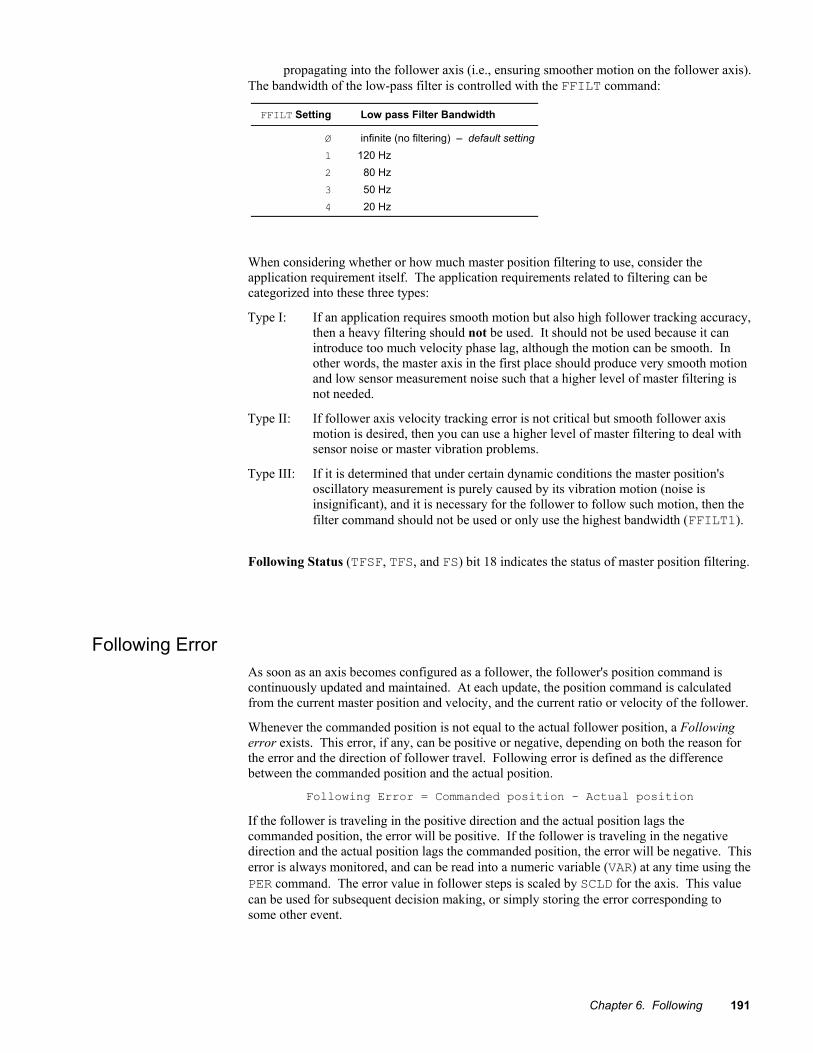
Chapter 6. Following 191
propagating into the follower axis (i.e., ensuring smoother motion on the follower axis). The bandwidth of the low-pass filter is controlled with the FFILT command:
FFILT Setting Low pass Filter Bandwidth
Ø infinite (no filtering) – default setting 1 120 Hz 2 80 Hz 3 50 Hz 4 20 Hz
When considering whether or how much master position filtering to use, consider the application requirement itself. The application requirements related to filtering can be categorized into these three types:
Type I: If an application requires smooth motion but also high follower tracking accuracy, then a heavy filtering should not be used. It should not be used because it can introduce too much velocity phase lag, although the motion can be smooth. In other words, the master axis in the first place should produce very smooth motion and low sensor measurement noise such that a higher level of master filtering is not needed.
Type II: If follower axis velocity tracking error is not critical but smooth follower axis motion is desired, then you can use a higher level of master filtering to deal with sensor noise or master vibration problems.
Type III: If it is determined that under certain dynamic conditions the master position's oscillatory measurement is purely caused by its vibration motion (noise is insignificant), and it is necessary for the follower to follow such motion, then the filter command should not be used or only use the highest bandwidth (FFILT1).
Following Status (TFSF, TFS, and FS) bit 18 indicates the status of master position filtering.
Following Error As soon as an axis becomes configured as a follower, the follower's position command is continuously updated and maintained. At each update, the position command is calculated from the current master position and velocity, and the current ratio or velocity of the follower.
Whenever the commanded position is not equal to the actual follower position, a Following error exists. This error, if any, can be positive or negative, depending on both the reason for the error and the direction of follower travel. Following error is defined as the difference between the commanded position and the actual position.
Following Error = Commanded position - Actual position
If the follower is traveling in the positive direction and the actual position lags the commanded position, the error will be positive. If the follower is traveling in the negative direction and the actual position lags the commanded position, the error will be negative. This error is always monitored, and can be read into a numeric variable (VAR) at any time using the PER command. The error value in follower steps is scaled by SCLD for the axis. This value can be used for subsequent decision making, or simply storing the error corresponding to some other event.
192 6K Series Programmer’s Guide
Maximum Velocity and Acceleration (Stepper Axes Only) The follower's attempt to faithfully follow the master can command velocities and accelerations that the follower axis is physically not able to complete. Therefore, the FMAXV and FMAXA commands are provided to set the maximum velocity and acceleration at which the follower will be allowed to move.
If the follower is commanded to move at rates beyond the defined maximums, the follower will begin falling behind it's commanded position. If this happens, a correction velocity will be applied to correct the position error as soon as the commanded velocity and acceleration fall within the limitation of FMAXV and FMAXA.
The FMAXA and FMAXV commands should be used only to protect against worst case conditions, and should be avoided altogether if they are not needed. If an axis is not able to follow its profile because of limitations imposed by these commands, some correction motion will occur. If the maximum acceleration (FMAXA value) is set very low, some oscillation about the commanded position can occur because the follower is not allowed to decelerate fast enough to prevent overshoot.
Factors Affecting Following Accuracy There are additional accuracy requirements of Following applications beyond those of standard positioning. The follower axis must maintain positioning accuracy while in motion, not just at the end of moves, because it is trying to stay synchronized with the master.
Assuming parameters such as master and follower scaling and ratios have been specified correctly, the overall positioning accuracy for an application depends on several factors:
• Resolution of the master • Resolution of the follower axis • Position sampling accuracy • Accuracy of the follower axis motor and drive • Accuracy of load mechanics • Master position prediction • Master velocity relative to master position prediction & master position filtering • Tuning (servo axes only) • Repeatability of the trigger inputs and sensors
Just as with a mechanical arrangement, the accuracy errors can build up with every link from the beginning to the end. The overall worst case accuracy error will be the sum of all the sources of error listed below. The errors fall into two broad categories, namely, master measurement errors and follower errors. These both ultimately affect follower accuracy, because the commanded follower position is based on the measured master position.
It is important to understand how master measurement errors result in follower position errors. In many applications, master and follower units will be the same (e.g., inches, millimeters, degrees). These applications will require linear speeds or surface speeds to be matched (i.e., a 1:1 ratio). For example, suppose that in a rotary knife application, there were 500 master steps per inch of material, so an error in master measurement of one encoder step would result in 0.002 inches of follower position error.
If the master and follower units are not the same, or the ratio is not 1:1, the master error times the ratio of the application gives the follower error. An example would be a rotary master and a linear follower. For instance, suppose one revolution of a wheel gives 4000 master counts, and results in 10 inches of travel on the follower. The ratio is then 10 inches/revolution. The follower error that results from one step of master measurement error is (1/4000) ∗ 10 inches/revolution = 0.0025 inches.

Chapter 6. Following 193
Resolution of the Master
The best case master measurement precision is the inverse of the number of master steps per user's master unit. For example, if there are 100 master steps/inch, then the master measurement precision is 0.01 inches. Even if all other sources of error are eliminated, follower accuracy will only be that which corresponds to 1 step of the master (e.g., 0.01 inches in the previous example).
Resolution of the Follower
The best case follower axis precision is the inverse of the number of follower steps per user's position unit. For example, if there are 1000 follower steps/inch, then the follower resolution is 0.001 inches. Even if all other sources of error are eliminated, follower positioning accuracy will only be that which corresponds to 1 step of the follower. This must be at least as great as the precision required by the application.
Position Sampling Accuracy
The position sampling rate for the 6K controller depends on whether it is a servo or a stepper. The sample period for is 2 ms.
The repeatability of the sampling rate, from one sample to the next, can vary by as much as 100 µs. This affect can be eliminated by using non-zero master position filter (FFILT) command values. Otherwise, measurement of master position can be off by as much as (20 to 100 microseconds ∗ master speed). This can appear to be a significant value at high master speeds, but it should be noted that this error changes in value (and usually sign) every sample period. It is effectively like a noise of 200-600 Hz; if the mechanical frequency response of the motor and load is much less than this frequency, the load cannot respond to this error.
Accuracy of the Follower Motor and Drive
The precision also depends on how accurately the drive follows its commanded position while moving. Even if master measurement were perfect, if the drive accuracy is poor, the precision will be poor.
In the case of stepper drives, this amounts to the specified motor/drive accuracy.
In the case of servo drives, the better the drive is tuned for smoothness and zero Following error, the better the precision of the positioning. Often, this really only matters for a specific portion of the profile, so the drive should be tuned for zero Following error at that portion.
Accuracy of the Load Mechanics
The accuracy (not repeatability) of the load mechanics must be added to the overall build up of accuracy error. This includes backlash for applications that involve motion in both directions.
Master Position Prediction
The master position prediction mode can be enabled or disabled with the FPPEN command, but each state contributes a different error.
Disabled (FPPENØ): The follower position command is based on a master position that is 2 sample periods (4 ms) old. This means that master measurement error due to disabling the position prediction mode will be (2 sample periods ∗ master speed).
Enabled (FPPEN1): If the position prediction mode is enabled (default setting), its accuracy is also affected by position sampling accuracy, master speed, and master position filtering. The error due to enabling the position prediction mode is about twice that due to sampling accuracy (i.e., 40 to 200 microseconds ∗ master speed). As with the error due to position sampling accuracy, the error due to the position prediction mode being enabled is like a noise on the order of 200-600 Hz, which is not noticed by large loads.

194 6K Series Programmer’s Guide
Master Velocity Relative to Master Position Prediction
Variation in Master Velocity: Although increasing master position filtering (increasing the FFILT command value) eliminates the error due to sampling accuracy, it increases the error due to variations in master speed when the master position prediction mode is enabled (FPPEN1).
Most applications maintain a constant master speed, or change very slowly, so this effect is minimal. But if the master is changing rapidly, there can be a significant master speed measurement error. Because predicted master positions are in part based on master speed measurement, the can result in an error in master position prediction mode (FPPEN1). This effect will always be smaller than that due to the master position prediction mode being disabled (FPPENØ).
Tuning (Servo Axes Only)
A servo system’s tuning has a direct impact on how well the follower axis can track the master input. Overshoot, lag, oscillation, etc., can be devastating to Following performance. The best tool to use for tuning the 6K series controller is Motion Planner’s Servo Tuner utility.
Repeatability of the Trigger Inputs and Sensors
Some applications can use the trigger inputs for functions like registration moves, GOWHENs, or new cycles. For these applications, the repeatability of the trigger inputs and sensors add to the overall position error.
Refer to page 84 for accuracy specifications on the trigger input position capture function. Refer to your sensor manufacturer’s documentation for the sensor repeatability.
Preset vs. Continuous Following Moves When a follower performs a preset (MCØ) move in Following mode (FOLEN1), the commanded position is either incremental or absolute in nature, but it does have a commanded endpoint. The direction traveled by the follower will be determined by the commanded endpoint position, and the direction the master is counting.
Let’s illustrate this with an example. Assume all necessary set-up commands have been previously issued for our follower (axis 1) and master so that distances specified are in revolutions:
FOLRN3 ; Set Following follower-to-master ratio numerator to 3 FOLRD4 ; Set Following follower-to-master ratio denominator to 4 ; (ratio is 3 revs on the follower to 4 revs on the master) FOLEN1 ; Enable Following on axis 1 FOLMD10 ; Set preset move to take place over 10 master revolutions MC0 ; Set follower to preset positioning mode MA1 ; Set follower to absolute positioning mode PSET0 ; Set current absolute position reference to zero D5 ; Set move distance to absolute position 5 revolutions GO1 ; Initiate move to absolute position 5
If the master is stationary when the GO1 command is executed, the follower will remain stationary also. If the master begins to move and master pulses are positive in direction, the follower will begin the preset move in the positive direction. If the master pulses stop arriving before 10 master revolutions have been traveled, the follower will also stop moving, but that GO1 command will not be completed. If the master then starts to count in the negative direction, the follower will follow in the negative direction, but only as far as it's starting position. If the master continues to count negative, the follower will remain stationary. The GO1 command will not actually be completed until the master has traveled at least 10 revolutions in the positive direction from where it was at the time the GO1 command was executed. If the master oscillates back and forth between it's position at the start of the GO1 command to just under 10 revolutions, the follower will oscillate back and forth as well.
The master must be counting in the positive direction for any preset (MCØ) GO1s commanded

Chapter 6. Following 195
on the follower to be completed. If mechanics of the system dictate that the count on the source of the master pulses is negative, a minus (-) sign should be entered in the FOLMAS command so that 6K controller sees the master counts as positive.
Continuous follower moves (MC1) react much differently to master pulse direction. Whereas a preset move will only start the profile if the master counts are counting in the positive direction, a continuous move will begin the ramp to its new ratio following the master in either direction. As long as the master is counting in the positive direction, the direction towards which the follower starts in a continuous move is determined by the argument (sign) of the D command. The follower direction is positive for D+ and negative for D-.
If the master is counting in the negative direction when follower begins a continuous move, the direction towards which the follower moves is opposite to that commanded with the D command. The follower direction is positive for D- and negative for D+.
If the master changes direction during a continuous follower move, the follower will also reverse direction. As with standard continuous moves, the GO1 will continue until terminated by S, K, end-of-travel limits, stall condition, or command to go to zero velocity. As with preset moves, the sign on the FOLMAS command determines the direction of master counting with respect to the direction of actual counting on the master input.
Master and Follower Distance Calculations The formulas below show the relationship between master move distances and the corresponding follower move distances. These relationships can be used to assist in the design of Following mode moves in which both the position and duration of constant ratio are important.
In such calculations, it is helpful to use SCLMAS and SCLD values that allow the master and follower distances to be expressed in the same units (e.g., inches or millimeters). In this case, many applications will be designed to reach a final ratio of 1:1, and the distances in these figures can be easily calculated.
HINT: For a trapezoidal preset follower axis move with a maximum ratio of 1:1, the master and follower distances during the constant ratio portion will be the same. The follower travel during acceleration will be exactly half of the corresponding master travel, and it will also occur during deceleration.
Master Distance (FOLMD) If the follower axis is in continuous positioning mode (MC1), FOLMD is the master distance over which the follower axis is to accel or decel from the current ratio to the new ratio. If the follower axis is in preset positioning mode (MCØ), FOLMD is the master distance over which the follower's entire move will take place.
When the Follower is in Continuous Positioning Mode (MC1)
D = FOLMD * (R2 + R1)
2
where: FOLMD = Master distance R2 = New ratio (FOLRN ÷ FOLRD) R1 = Current ratio (FOLRN ÷ FOLRD) D = Follower distance traveled during ramp

196 6K Series Programmer’s Guide
When the Follower is in Preset Positioning Mode (MCØ)
Trapezoidal Follower Moves
Dmax = (FOLMD * Rmax)
D1 = (Dmax - D)
2
MD1 = 2 * D1Rmax
D2 = D - (2 * D1)
MD2 = D2Rmax
FOLMD = 2 * MD1) + MD2
where: FOLMD = Master distance MD1 = Master distance during accel & decel ramps MD2 = Master distance during constant ratio D = Total follower axis preset distance commanded D1 = Follower travel during accel and decel ramps D2 = Follower travel during constant ratio Dmax = Maximum follower distance possible
(assuming no accel or decel) Rmax = Maximum ratio = FOLRN ÷ FOLRD
R max
Distance
Trapezoidal profile if:D = (D2 + 2 * D1) < Dmax
Rectangular profile if:D 2 = DD 1 = zeroMD 2 = FOLMDMD 1 = zero
R max
Distance
D2
D1 D2 D1
MD1 MD2 MD1
MD2
Rat
ioR
atio
Triangular Follower Moves
D = Rpeak * FOLMD
2
where: FOLMD = Master distance Rpeak = Peak ratio reached during move D = Total follower distance
R max
Distance
Triangular profile if:D < 1/2 D max
D
Rpeak
Rat
io
FOLMD
Distance Calculation Example
In the example below, the desired travel during constant ratio is already contained in numeric variable 1 (VAR1), and can have been read from thumbwheels or a DATA command. The corresponding follower move distance (D) and FOLMD are calculated as shown:
VAR2=2 ; Desired follower travel during accel and decel combined VAR3=2 * VAR2 ; Required master travel during these ramps VAR4=VAR1 + VAR2 ; Move distance is constant ratio portion plus ramps VAR5=VAR1 + VAR3 ; Master travel for entire follower move FOLMD(VAR5) ; Establish calculated master travel D(VAR4) ; Establish calculated follower travel GO1 ; Make desired follower move
Similar calculations can be done for a series of continuous move ramps to ratios, separated by GOWHEN for master cycle positions. These ramps can be repeated in a loop to create a continuous cyclical follower profile.
These Profiles depict ratio vs. distance
This Profile depicts ratio vs. distance

Chapter 6. Following 197
Beware of Roundoff Error (Scaling only)
Some potential for roundoff error exists if the scaling of a move distance or master distance by SCLD and SCLMAS does not result in an integer number of steps. Some additional care must be taken in the segment by segment construction of profiles using ramps to continuous ratio. The 6K controller maintains a follower position command that is calculated from the commanded constant ratios, the ramps to the new ratios, and the master travel over which these take place. At the end of each ramp or constant ratio portion, this commanded position is calculated to the nearest integer follower step. If the ratios and master travel result in a non-integer follower travel for a segment, the fractional part of that segment's calculated travel will be lost. In a cyclical application, repeated truncations could build up to a significant error. This can be avoided through careful attention to design of the profile.
Using Other Features with Following The 6K controller has many features that can be used in the same application as its Following features. In some cases, having configured an axis as a follower with the FOLMAS command will affect, or be affected by, the operation of other features, as described below.
Setups used by FOLMAS (Stepper Axes Only)
The FOLMAS command uses the drive resolution (DRES) and the velocity range (PULSE) data to configure an axis as a follower. In order for this data to be used correctly, these commands must be given before FOLMAS. These commands are not allowed after FOLMAS is given. After FOLMAS is executed, the MC command can be used to change from incremental to absolute positioning and back.
S (Stop) & K (Kill) Commands
Stop (S) and Kill (K) commands cause the follower to do a non-Following decel, even if the follower is in Following mode. A stop or a kill, buffered or immediate, will clear a pending GOWHEN condition (clears AS bit 26).
Kill Conditions Under default operation (FOLK0), certain error conditions (i.e., drive fault input active, or maximum position error limit exceeded) will cause the 6K controller to disable the drive and kill the Following profile (follower’s commanded position loses synchronization with the master).
If you enable Following Kill (FOLK1), these error conditions will still disable the drive (DRIVE0), but will not kill the Following profile. Because the Following profile is still running, the controller keeps track of what the follower’s position should be in the Following trajectory. To resume Following operation, resolve the error condition (drive fault, excessive position error), enable the drive (DRIVE1), and command the controller to impose a shift to compensate for the lapse/shift that occurred while the drive was disabled and the follower was not moving. To impose the shift, assign the negative of the internally monitored shift value (PSHF) to a variable (e.g., VAR1 = -1 * PSHF) and command the shift using a variable substitution in the FSHFD command (e.g., FSHFD(VAR1)).
The FOLK command only preserves Following profiles; normal velocity-based profiles will be killed regardless of the FOLK command.
GO Command If a follower axis is in Following mode (FOLEN1), moves will ramp to a ratio (set with FOLRN and FOLRD). If it is not in Following mode, moves will ramp to a velocity (V). Switching in and out of Following mode does not change the value for final ratio or final velocity goals, but simply changes which parameter is used as the goal.
Registration Moves (see page 155)
Registration inputs can be enabled with the INFNCi-H command while an axis is a follower, and registration moves can interrupt either a Following mode move or a time-based move. The registration move itself, however, is always a time based move, and implements the registration velocity with respect to a stationary reference. Any trigger input can be used as a registration input or for any Following feature that uses triggers, even at the same time.

198 6K Series Programmer’s Guide
Enter/Exit Following Mode While Moving
The FOLENØ command can be executed while a follower axis is moving at constant ratio. In this case, the current velocity becomes the constant velocity, and the follower can accelerate or decelerate to other velocities. The FOLEN1 command cannot be executed while the follower axis is moving in the non-Following mode. Attempting to do so will result in the error response “MOTION IN PROGRESS”.
Pause and Continue
A program can be paused and continued, even if one or more axes is configured as a follower axis. Those axes do not lose track of the master input, even though motion is stopped. As usual, if a program finishes normally, or if COMEXS is set to zero (COMEXSØ), the program cannot be continued. If a program is resumed, partially completed Following moves will be completed; however, the remainder of the move is completed over the entire original master distance (FOLMD value).
TVEL and TVELA Commands
The TVEL and VEL commands have always reported an unsigned value (i.e. magnitude), consistent with the fact that the V command is always positive, even if the move direction is negative. When Following is enabled (FOLEN1), TVEL and VEL report the net magnitude of commanded velocity due to following and/or shifting. For example, if the follower axis is Following in the positive direction at 1 rps, TVEL reports 1.000. If a shift in the negative direction of 1.5 rps is then commanded, TVEL will report 0.5 – still positive, even though the net direction is negative.
By contrast, TVELA and VELA have always been signed. In the above example, TVELA will report -0.5.
TASF, TAS & AS Axis Status Bits
Axis Status (TASF, TAS and AS) bits 1-4 represent the motion status of an axis. Bits 1 and 2 represent the moving and direction status of the net motion of an axis, including the combination of following and shifting.
Bits 3 and 4 represent acceleration and velocity, respectively. With Following disabled (FOLENØ), the accel and velocity can only be due to a commanded time-based profile. With Following enabled (FOLEN1), the net commanded velocity and accel could be due to following the master and/or a simultaneous shift (time-based profile). Bits 3 and 4 only reflect the acceleration and velocity status of the time-based profile, not the combined command.
For example, if the follower axis is Following in the positive direction at 1 rps, TAS reports 1ØØØ. If a continuous shift (FSHFC2) of 0.8 rps in the negative direction is then commanded, TAS will report 1Ø1Ø, while the shaft is decelerating to 0.2 rps. When the continuous shift velocity is reached, TAS will report 1ØØ1.
Changing Feedback Sources (Servo Axes only)
Changing feedback sources (SFB) can result in a follower axis Following its own feedback. For this reason, changing feedback sources is not allowed while a master is specified (FOLMAS).
Following and Other Motion
Following motion is initiated with the GO command, just like normal motion. Other motion, that does not depend on the motion of an external master, cannot be used while a follower axis is in Following mode (FOLEN1). These motion types include jog mode, joystick mode, contouring, homing, streaming mode, and linear interpolation (GOL). To use these motion types, Following must be disabled (FOLENØ) — see Enter/Exit Following Mode While Moving above for precautions.
Conditional Statements Using PMAS
The master cycle position (PMAS) value can be used in the comparison argument of these commands:
• WAIT & GOWHEN: If it is desired to WAIT or GOWHEN on a master cycle position of the next master cycle, one master cycle length (value of FMCLEN) should be added to the master cycle position specified in the argument. This allows commands that sequence

Chapter 6. Following 199
follower axis events through a master cycle to be placed in a loop. The WAIT or GOWHEN command at the top of the loop could execute, even though the actual master travel had not finished the previous cycle. This is done to allow a PMAS value that is equal to the master cycle length to be specified and reliably detected.
• IF, UNTIL, & WHILE: These arguments use the instantaneous PMAS value. Be careful to avoid specifying PMAS values that are nearly equal to the master cycle length (FMCLEN), because rollover can occur before a PMAS sample is read.
Compiled Motion Following profiles can be pre-compiled to save processing time. For details, see page 139.
Troubleshooting for Following (also see Chapter 8) The table below offers some possible reasons for troubles that can be encountered in achieving the desired follower motion.
Symptom Possible Causes Follower axes do not follow master • Improper FOLMAS
• Poor connection if master is encoder • Master running backward • No encoder power (when the encoder is selected as the master)
Follower motion is rough • FFILT command value too low • Unnecessary FPPEN amplifies master roughness
Ratio seems wrong • FOLRN and FOLRD follower-to-master ratio values are inaccurate, possibly reversed
• SCLD or SCLMAS wrong • Following limited by FMAXV or FMAXA (steppers only)
Follower profile wrong, or un-repeatable
• WAIT used where GOWHEN should be • Too little master travel between GOWHEN and GO1, desired PMAS is missed
Master/follower alignment drifts over many cycles
• Roundoff error due to fractional steps resulting from SCLD or SCLMAS and user's parameters
• Ratios and master distances specified result in fractional follower steps covered during ramps, constant ratio
Follower lags Following position (steppers only)
• Inhibited by FMAXV • FMAXA clips acceleration peaks resulting from attempt to follow rough master
Error Messages If an illegal programming condition is discovered while programming or executing programs, the 6K controller responds with an error message. If a program execution error is detected, the program is aborted.
The table below lists all the error messages that relate to Following, and indicates the command and cause that can generate them. These error messages are displayed only if the error level is set to level 4 with the ERRLVL4 command (this is the default setting).
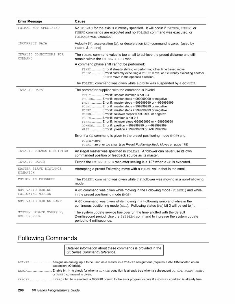
200 6K Series Programmer’s Guide
Error Message Cause
FOLMAS NOT SPECIFIED No FOLMAS for the axis is currently specified. It will occur if FMCNEW, FSHFC, or FSHFD commands are executed and no FOLMAS command was executed, or FOLMASØ was executed.
INCORRECT DATA Velocity (V), acceleration (A), or deceleration (AD) command is zero. (used by FSHFC & FSHFD)
INVALID CONDITIONS FOR COMMAND
The FOLMD command value is too small to achieve the preset distance and still remain within the FOLRN/FOLRD ratio. A command phase shift cannot be performed: FSHFD .............Error if already shifting or performing other time based move. FSHFC .............Error if currently executing a FSHFD move, or if currently executing another
FSHFC move in the opposite direction.
The FOLEN1 command was given while a profile was suspended by a GOWHEN.
INVALID DATA The parameter supplied with the command is invalid. FFILT .............Error if: smooth number is not 0-4 FMCLEN...........Error if: master steps > 999999999 or negative FMCP ...............Error if: master steps > 999999999 or <-999999999 FOLMD .............Error if: master steps > 999999999 or negative FOLRD .............Error if: master steps > 999999999 or negative FOLRN .............Error if: follower steps>999999999 or negative FSHFC .............Error if: number is not 0-3 FSHFD .............Error if: follower steps>999999999 or <-999999999 GOWHEN...........Error if: position > 999999999 or <-999999999 WAIT ...............Error if: position > 999999999 or <-999999999
Error if a GO command is given in the preset positioning mode (MCØ) and: FOLRN = zero FOLMD = zero, or too small (see Preset Positioning Mode Moves on page 175)
INVALID FOLMAS SPECIFIED An illegal master was specified in FOLMAS. A follower can never use its own commanded position or feedback source as its master.
INVALID RATIO Error if the FOLRN:FOLRD ratio after scaling is > 127 when a GO is executed.
MASTER SLAVE DISTANCE MISMATCH
Attempting a preset Following move with a FOLMD value that is too small.
MOTION IN PROGRESS The FOLEN1 command was given while that follower was moving in a non-Following mode.
NOT VALID DURING FOLLOWING MOTION
A GO command was given while moving in the Following mode (FOLEN1) and while in the preset positioning mode (MCØ).
NOT VALID DURING RAMP A GO command was given while moving in a Following ramp and while in the continuous positioning mode (MC1). Following status (FS) bit 3 will be set to 1.
SYSTEM UPDATE OVERRUN, USE SYSPER4
The system update service has overrun the time allotted with the default 2-millisecond period. Use the SYSPER4 command to increase the system update period to 4 milliseconds.
Following Commands Detailed information about these commands is provided in the 6K Series Command Reference.
ANIMAS .......................... Assigns an analog input to be used as a master in a FOLMAS assignment (requires a ANI SIM located on an expansion I/O brick).
ERROR............................. Enable bit 14 to check for when a GOWHEN condition is already true when a subsequent GO, GOL, FGADV, FSHFC, or FSHFD command is given.
ERRORP .......................... If ERROR bit 14 is enabled, a GOSUB branch to the error program occurs if a GOWHEN condition is already true

Chapter 6. Following 201
when a subsequent GO, GOL, FGADV, FSHFC, or FSHFD command is given. FFILT............................. Sets the bandwidth for master position filtering. FGADV............................. Defines the geared advance distance. FMAXA............................. Stepper axes only: Sets the maximum acceleration a follower can use while Following. FMAXV............................. Stepper axes only: Sets the maximum velocity at which a follower can travel. FMCLEN .......................... Defines the length of the master cycle. FMCNEW .......................... Restarts new master cycle counting immediately. To make this a trigger-based operation instead of issuing the
FMCNEW command, use the TRGFNcx1 command. FMCP............................... Defines the initial position of a new master cycle. FOLEN............................. Enables or disables Following mode. FOLK............................... Allows drive fault or maximum position error to disable drive without killing the Following profile. FOLMAS .......................... Defines masters for follower axes. FOLMD............................. Defines the master distance over which ratio changes or moves are to take place. FOLRD............................. Establishes the DENOMINATOR ONLY for the maximum follower-to-master ratio for a preset move or the final
ratio for a continuous move (use in combination with the FOLRN command). FOLRN............................. Establishes the NUMERATOR ONLY for the maximum follower-to-master ratio for a preset move or the final ratio
for a continuous move (use in combination with the FOLRD command). FPPEN............................. Allows master position prediction to be enabled or disabled. FSHFC............................. Allows continuous advance or retard (shift) of follower position during continuous Following moves. FSHFD............................. Allows preset advance or retard (shift) of follower position during continuous Following moves. FVMACC .......................... Establishes the rate at which the virtual master count frequency (FVMFRQ) can change for an axis. FVMFRQ .......................... Defines the frequency of the virtual master count. GOWHEN .......................... A GOWHEN command suspends execution of the next follower move until the specified conditional statement
(based on T, IN, LIM, PC, PE, PMAS, PSLV, or PSHF) is true. To make this a trigger-based operation instead of issuing the GOWHEN command, use the TRGFNc1x command.
SCLD............................... Sets the follower distance scale factor. SCLMAS .......................... Sets the master scale factor. SINAMP .......................... Defines the amplitude of the internal sine wave. SINANG .......................... Defines the phase angle of the internal sine wave. SINGO............................. Initiates the internal sine wave. TRGFN............................. aTRGFNc1x initiates a GOWHEN. Suspends execution of the next follower move on follower axis (a) until the
specified trigger input (c) goes active. aTRGFNcx1 allows master cycle counting to be restarted on axis (a) when the specified trigger input (c) goes active.
Status and Assignment Commands TASF, TAS & [ AS ] ....... Bit 26 of each axis status is set (1) if a motion profile suspended by a GOWHEN (including TRGFNc1x) is pending on
that axis. The bit is cleared when the GOWHEN is true, or when a stop (S) or kill (K) command is executed. TERF, TER & [ ER ] ....... Bit 14 is set if the GOWHEN condition is already true when a subsequent GO, GOL, FGADV, FSHFC, or FSHFD
command is given. (The corresponding error-checking bits must be enabled with the ERROR command before the error will be detectable.)
TFSF, TFS & [ FS ] ....... Transfers or assigns/compares the Following status or each axis. TNMCY and [ NMCY ] ..... Transfers or assigns the current master cycle number. TPCMS and [ PCMS ] ..... Transfers or assigns the current captured master cycle position. TPMAS and [ PMAS ] ..... Transfers or assigns the current master cycle position. TPSHF and [ PSHF ] ..... Transfers or assigns the net position shift since constant ratio. TPSLV and [ PSLV ] ..... Transfers or assigns the follower's current commanded position. TVMAS and [ VMAS ] ..... Transfers or assigns the current velocity of the master axis. WAIT............................... A WAIT command suspends program execution until the specified conditional statement (based on PMAS, FS,
NMCY, PCMS, PSHF, PSLV, or VMAS) is true; WAIT(SS.i=b1) suspends program execution until a trigger input is activated (“i” is the input bit number corresponding to the trigger input—see the 6K Series Command Reference).


7
C H A P T E R S E V E N
Multi-Tasking
IN THIS CHAPTER • Introduction to Multi-Tasking .........................................................................204 • Using 6K Resources While Multi-Tasking......................................................213 • Multi-Tasking Performance Issues..................................................................217 • Multi-Tasking Application Examples .............................................................219
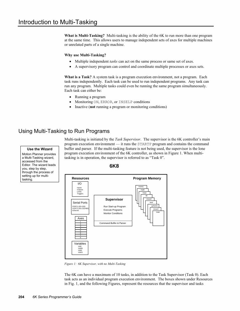
204 6K Series Programmer’s Guide
Introduction to Multi-Tasking
What is Multi-Tasking? Multi-tasking is the ability of the 6K to run more than one program at the same time. This allows users to manage independent sets of axes for multiple machines or unrelated parts of a single machine.
Why use Multi-Tasking? • Multiple independent tasks can act on the same process or same set of axes. • A supervisory program can control and coordinate multiple processes or axes sets.
What is a Task? A system task is a program execution environment, not a program. Each task runs independently. Each task can be used to run independent programs. Any task can run any program. Multiple tasks could even be running the same program simultaneously. Each task can either be:
• Running a program • Monitoring ON, ERROR, or INSELP conditions • Inactive (not running a program or monitoring conditions)
Using Multi-Tasking to Run Programs
Use the Wizard Motion Planner provides a Multi-Tasking wizard, accessed from the Editor. The wizard leads you, step by step, through the process of setting up for multi-tasking.
Multi-tasking is initiated by the Task Supervisor. The supervisor is the 6K controller’s main program execution environment — it runs the STARTP program and contains the command buffer and parser. If the multi-tasking feature is not being used, the supervisor is the lone program execution environment of the 6K controller, as shown in Figure 1. When multi-tasking is in operation, the supervisor is referred to as “Task 0”.
Resources
Variables
Serial Ports
Axes
I/O
12345678
Program Memory
move1
math
inout
move2
fill
seal
gohome
move3
main
Supervisor
Run Start-up Program
Execute Programs
Monitor Conditions
Command Buffer & Parser
6K8
VARVARBVARIVARS
PORT1 (RS-232)PORT2 (RS-232/485)Ethernet
InputsOutputsLimitsTriggers
Figure 1: 6K Supervisor, with no Multi-Tasking
The 6K can have a maximum of 10 tasks, in addition to the Task Supervisor (Task 0). Each task acts as an individual program execution environment. The boxes shown under Resources in Fig. 1, and the following Figures, represent the resources that the supervisor and tasks

Chapter 7. Multi-Tasking 205
monitor and manipulate (see list below). These resources can be shared with other tasks. • I/O................................. Inputs and Outputs (onboard I/O and expansion I/O bricks) • Communication ports ... “RS-232”, “RS-232/485”, and “ETHERNET” • Axes.............................. Axes available with the 6K • Variables ...................... Real (VAR), binary (VARB), integer (VARI), and string (VARS)
“Program Memory” is the 6K’s non-volatile memory where programs are stored. Any task can run any program. Multiple tasks could even be running the same program simultaneously. Programs in multi-tasking are defined as they typically are with the 6K
Resources Program Memory
move1
math
inout
move2
fill
seal
gohome
move3
main
Supervisor
Task 1
Task 2
Execute ProgramsMonitor Conditions
Execute ProgramsMonitor Conditions
Command Buffer & Parser
Run Start-up Program
Execute ProgramsMonitor Conditions
Execute ProgramsMonitor Conditions
Task 10
6K8
Variables
Serial Ports
Axes
I/O
12345678
VARVARBVARIVARS
PORT1 (RS-232)PORT2 (RS-232/485)Ethernet
InputsOutputsLimitsTriggers
Figure 2: 6K8 - Multi-Tasking with 10 tasks.
The Task Identifier (%) prefix is used to specify that the associated command will affect the indicated task number. For most simple multi-tasking applications, the % prefix will only be used to start a program running in a specific task. Multi-tasking programs can be started through the communication ports (see Figs. 3a-3c), or from a program (see Figs. 4a-4d). Note that the programs are run in the tasks specified with the % prefix.
Starting Tasks from a Communications Port Resources
Variables
Serial Ports
Axes
I/O
12345678
Program Memory
move1
Supervisor
Task 1
6K8
Ethernet
1%move1
1%move1
1%move1
1%move1
DEF move1___
ENDRun move1
Figure 3a: Multi-Tasking initiated from a computer terminal.

206 6K Series Programmer’s Guide
Resources
Variables
Serial Ports
Axes
I/O
12345678
Program Memory
move1
Supervisor
Task 1
6K8
Ethernet
2%inout
2%inout
2%inout
2%inout
DEF move1___
END
inout
DEF inout___
END
Running move1
Task 2
Run inout
Figure 3b: Multi-Tasking initiated from a computer terminal (cont’d).
Resources
Variables
Serial Ports
Axes
I/O
12345678
Program Memory
move1
Supervisor
Task 1
6K8
Ethernet
3%fill
3%fill
3%fill
3%fill
DEF move1___
END
inout
DEF inout___
END
Running move1
Task 2
Running inout
Task 3
Run fill
fill
DEF fill___
END
Figure 3c: Multi-Tasking initiated from a computer terminal (cont’d).
Starting Tasks from a Program
Resources
Variables
Serial Ports
Axes
I/O
12345678
Program Memorymain
Supervisor
6K8
Ethernet
RUN main
RUN mainRUN main
DEF main___
1%move12%inout3%fillEND
Figure 4a: Multi-Tasking initiated from a program.

Chapter 7. Multi-Tasking 207
Resources
Variables
Serial Ports
Axes
I/O
12345678
Program Memorymain
Supervisor
Task 1
6K8
Ethernet
Running main
1%move1
1%move1
1%move1 DEF main___
1%move12%inout3%fillEND
RUN move1
move1
DEF move1___
END
Figure 4b: Multi-Tasking initiated from a program (cont’d).
Resources
Variables
Serial Ports
Axes
I/O
12345678
Program Memorymain
Supervisor
6K8
Ethernet
Running main
2%inout
2%inout DEF main___
1%move12%inout3%fillEND
move1
DEF move1___
END
inout
DEF inout___
END
Task 1
2%inout
Running move1
Task 2
RUN inout
Figure 4c: Multi-Tasking initiated from a program (cont’d).
Resources
Variables
Serial Ports
Axes
I/O
12345678
Program Memorymain
Supervisor
6K8
Ethernet
Running main
3%fill
3%fill DEF main___
1%move12%inout3%fillEND
move1
DEF move1___
END
inout
DEF inout___
END
fill
DEF fill___
END
Task 1
Running move1
Task 2
Running inout
3%fill
Task 3
RUN fill
Figure 4d: Multi-Tasking initiated from a program (cont’d).

208 6K Series Programmer’s Guide
Interaction Between Tasks A new task is initiated by identifying the task number with the Task Identifier (%) prefix, followed by the name of the program to be run in the specified task. Because the % prefix specifies the task number that the associated command will affect, new tasks can be started from within other tasks. Fig. 5b shows the move1 program in task 1 being started by the main program in the supervisor. Fig. 5c shows the fill program in task 3 being started by the move1 program in task 1 with the 3%fill command. Fig. 5d shows the inout program in task 2 being started by the fill program in task 3 with the 2%inout command.
Program execution in a task is controlled by commands executed from the program the task is running. In the example shown in Figs 5a-5d, program execution in Task 1 is controlled by commands executed from the move1 program, program execution in Task 2 is controlled by commands executed from the inout program, and program execution in Task 3 is controlled by commands executed from the fill program.
Resources
Variables
Serial Ports
Axes
I/O
12345678
Program Memorymain
Supervisor
6K8
Ethernet
RUN main
RUN mainRUN main
DEF main1%move1___
END
Figure 5a: Initiating multi-tasking.
Resources
Variables
Serial Ports
Axes
I/O
12345678
Program Memorymain
Supervisor
Task 1
6K8
Ethernet
Running main
1%move1
1%move1
1%move1DEF main1%move1___
END
RUN move1
move1DEF move13%fill__
END
Figure 5b: Task initiated from another task (cont’d).

Chapter 7. Multi-Tasking 209
Resources
Variables
Serial Ports
Axes
I/O
12345678
Program Memorymain
Supervisor
6K8
Ethernet
Running mainDEF main1%move1___
END
move1DEF move13%fill__
END
fill
DEF fill2%inout__
END
Task 1
Running move1
3%fill
3%fill
3%fill
Task 3
RUN fill
Figure 5c: Task initiated from another task (cont’d).
Resources
Variables
Serial Ports
Axes
I/O
12345678
Program Memorymain
Supervisor
6K8
Ethernet
Running mainDEF main1%move1___
END
move1DEF move13%fill__
END
inout
DEF inout___
END
fill
DEF fill2%inout__
END
Task 1
Running move1
Task 2
RUN inout2%inout
2%inout 2%inout
Task 3
Running fill
Figure 5d: Task initiated from another task (cont’d).

210 6K Series Programmer’s Guide
Axes & Tasks
Refer to page 213 for more details about
associating axes with tasks.
The default condition in multi-tasking is that each task is associated with all controller axes, as shown in Fig. 6a. This means that when an axis being used in a task hits an end-of travel limit, program execution will be killed within that task, and in all other tasks, because they all share that axis. It can therefore be necessary to assign a set of axes to a given task to allow a multi-axis controller to be used as more than one independent program execution environment.
The TSKAX command allows you to assign axes to specific tasks, thus constraining task response and control to a smaller set of axes. A task is allowed to control only its associated axes. This axis association covers all interaction between axes commands, conditions or inputs and task program flow. For example, if a 6K controller is controlling two independent machines that do not share common axes, with control of each machine as a separate task, a limit hit by an axis in one machine can kill the task running that machine, but will not kill the task running the other machine.
Default = All Axes
Resources Program Memory
move1
math
inout
move2
fill
seal
gohome
move3
main
Supervisor
Task 1
Task 2
Execute ProgramsMonitor Conditions
Execute ProgramsMonitor Conditions
Command Buffer & Parser
Run Start-up Program
Execute ProgramsMonitor Conditions
Execute ProgramsMonitor Conditions
Task 10
6K8
Variables
Serial Ports
Axes
I/O
12345678
VARVARBVARIVARS
PORT1 (RS-232)PORT2 (RS-232/485)Ethernet
InputsOutputsLimitsTriggers
Default = All Axes
Default = All Axes
Figure 6a: Each task is associated with all controller axes in default condition.
The TSKAX command syntax identifies the first and last axis numbers (range) associated with the task. Thus, the axes associated with a task will always be consecutive. For example, the following commands will associate axes 1-3 with Task 1, axes 4-6 with Task 2, and axes 7 and 8 with Task 3. These associations are illustrated in Figures 6b-6d below. If axis 3 in task 1 hits a limit, program execution in task 1 will be killed, but task 2 and task 3 can continue to run because they are independent and do not share axis 3. DEF main ; Begin definition of program called "main" 1%TSKAX1,3 ; Associate axes 1-3 with Task 1 (see Fig 6b) 2%TSKAX4,6 ; Associate axes 4-6 with Task 2 (see Fig 6c) 3%TSKAX7,8 ; Associate axes 7 & 8 with Task 3 (see Fig 6d) 1%move1 ; Execute the "move1" program in Task 1 (affects axes 1-3) 2%inout ; Execute the "inout" program in Task 2 (affects axes 4-6) 3%fill ; Execute the "fill" program in Task 3 (affects axes 7 & 8) END ; End definition of program called "main"
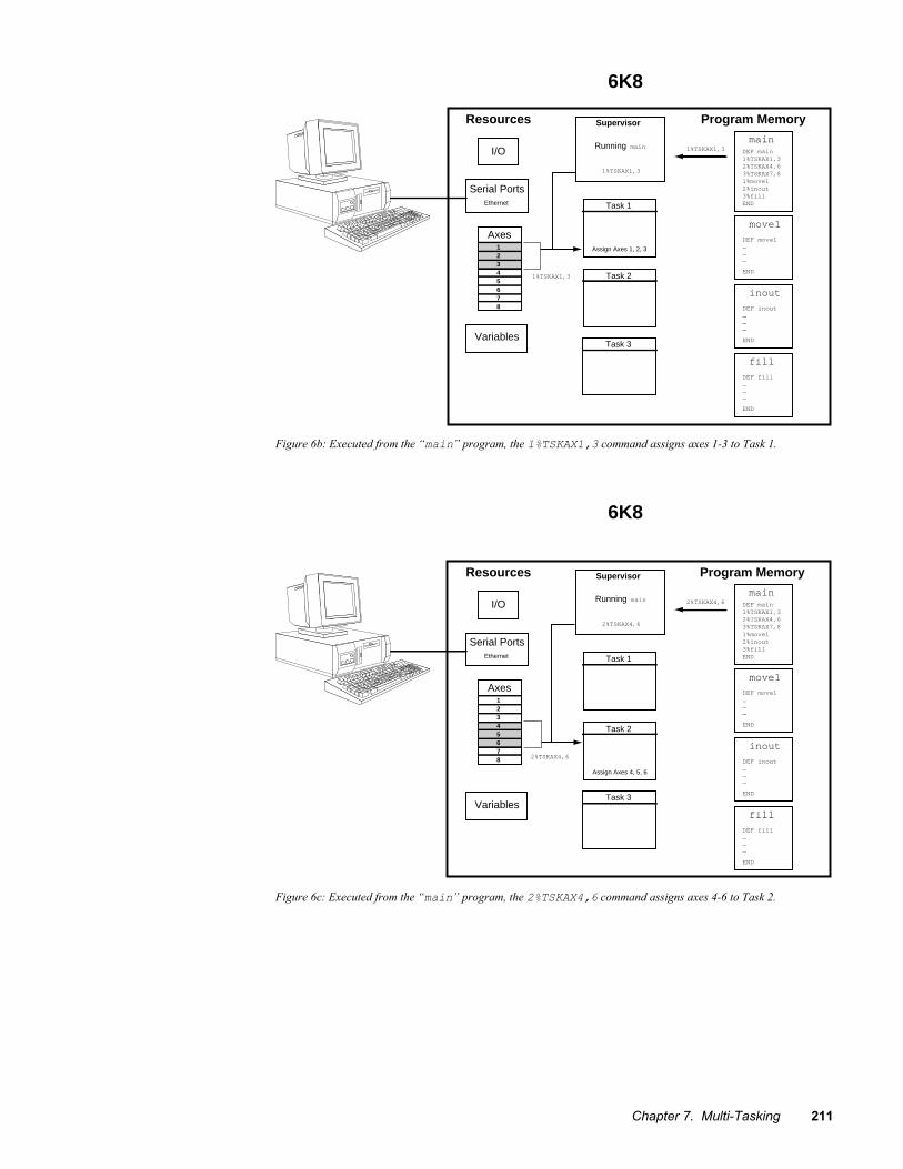
Chapter 7. Multi-Tasking 211
Resources
Variables
Serial Ports
Axes
I/O
12345678
Program Memorymain
Supervisor
6K8
Ethernet
1%TSKAX1,3
1%TSKAX1,3
1%TSKAX1,3
DEF main1%TSKAX1,32%TSKAX4,63%TSKAX7,81%move12%inout3%fillEND
move1
DEF move1___
END
inout
DEF inout___
END
fill
DEF fill___
END
Task 1
Task 2
Task 3
Assign Axes 1, 2, 3
Running main
Figure 6b: Executed from the “main” program, the 1%TSKAX1,3 command assigns axes 1-3 to Task 1.
Resources
Variables
Serial Ports
Axes
I/O
12345678
Program Memorymain
Supervisor
6K8
Ethernet
2%TSKAX4,6
2%TSKAX4,6
2%TSKAX4,6
DEF main1%TSKAX1,32%TSKAX4,63%TSKAX7,81%move12%inout3%fillEND
move1
DEF move1___
END
inout
DEF inout___
END
fill
DEF fill___
END
Task 1
Task 2
Task 3
Assign Axes 4, 5, 6
Running main
Figure 6c: Executed from the “main” program, the 2%TSKAX4,6 command assigns axes 4-6 to Task 2.

212 6K Series Programmer’s Guide
Resources
Variables
Serial Ports
Axes
I/O
12345678
Program Memorymain
Supervisor
6K8
Ethernet
3%TSKAX7,8
3%TSKAX7,8
3%TSKAX7,8
DEF main1%TSKAX1,32%TSKAX4,63%TSKAX7,81%move12%inout3%fillEND
move1
DEF move1___
END
inout
DEF inout___
END
fill
DEF fill___
END
Task 1
Task 2
Task 3
Assign Axes 7, 8
Axes 4, 5, 6
Axes 1, 2, 3
Running main
Figure 6d: Executed from the “main” program, the 3%TSKAX7,8 command assigns axes 7 and 8 to Task 3.
How a “Kill” Works While Multi-Tasking The general rule of command execution within a task is that the command affects only the task in which it was executed or to which it was directed via the % prefix. This includes almost all motion commands when tasks have associated (TSKAX) axes. The exception is the Kill command. A “K” or “!K” without prefix or parameters will kill all controller axes, and programs running in all tasks. This exception is made to allow one short, familiar command to effectively stop all controller processes. As usual, a “K” with parameters (e.g., Kx11) will kill motion only on the specified axes, and will not kill the program. A “K” prefixed with a task specifier but without parameters (e.g., 3%K) will kill the program and motion of all axes associated with that task.
Certain inputs can be used to kill programs and motion. These inputs and their results under multi-tasking are:
• Drive Fault input. Kills program execution and associated axes for all tasks that are associated with the faulted axis.
• Kill input (INFNCi-C or LIMFNCi-C). If prefixed with the task identifier (e.g., 2%INFNC3-C), it will kill the designated task, its program and associated axes. If not prefixed with a task identifier, it will kill all controller axes, and programs running in all tasks. It will also cause a branch to the task’s error program if the task’s error-checking bit 6 is enabled (n%ERROR.6-1).
• User fault input (INFNCi-F or LIMFNCi-F). This input functions the same as the kill input noted above, with the exception that it will also cause a branch to the task’s error program if the task’s error-checking bit 7 is enabled (n%ERROR.7-1).
Chapter 7. Multi-Tasking 213
Using 6K Resources While Multi-Tasking
Associating Axes with Tasks The default condition in multi-tasking is that each task is associated with all controller axes. The TSKAX command allows you to assign axes to specific tasks, thus constraining task response and control to a smaller set of axes. The TSKAX command allows you to specify the first and last axis numbers associated with the task; thus, the axes associated with a task will always be consecutive. This association covers all interaction between axes commands, conditions or inputs and task program flow, including the following:
• Axis data commands (e.g., A, V, D). These commands will affect only the associated axes. If data is supplied in the fields of non-associated axes, it will be ignored. To alter the data of an axis associated with another task, that task number must prefix the command (e.g., if axis 3 is associated with task 2 but not task 1, then to change axis 3 velocity to 5 units/sec from task 1, the command 2%3V5 can be issued).
• Stop, pause, and continue commands and inputs. These commands will affect motion only on the associated axes of the task receiving the command: S (stop) command — without parameters, PS (pause) command, and C (continue) command. Inputs programmed with these functions will affect motion only on the associated axes of the task specified in the input function assignment (with the n% prefix): Kill input (n%INFNCi-C or n%LIMFNCi-C), stop input (n%INFNCi-D or n%LIMFNCi-D), pause/continue input (n%INFNCi-E or n%LIMFNCi-E), and user fault input (n%INFNCi-F or n%LIMFNCi-F).
• Drive fault and limit inputs. If a drive fault or end-of-travel limit occurs on an axis, only tasks that include that axis as an associated axis will be killed.
• ON conditions. If user status information includes axis status bits, and ONUS is enabled via ONCOND, then only bits of an associated axis will be monitored by that task.
• ERROR conditions. Each task has its own error status register (ER, TER, TERF), error-checking bits (ERROR), and error program (ERRORP). If an axis-related error occurs, only the task that is associated (TSKAX) with the axis is affected.
• Command buffer control: − COMEXC. Pauses command processing of that task until no associated axes are
moving. − COMEXL. Allows specified associated axes to not kill that task’s program.
(COMEXL applies to axes, and any task that includes an axis will be affected by that axis’ COMEXL status. An axis can’t be enabled for one task and disabled for another.)
− COMEXR. Motion on only the associated axes will also pause if a task-specific pause input becomes active.
• OUTFNC bits. Output bits defined without an axis specifier will become active if the condition becomes true on any associated axis.

214 6K Series Programmer’s Guide
Sharing Common Resources Between Multiple Tasks Controller resources other than processing time must also be shared between multiple tasks. All physical inputs and outputs are shared (i.e., each task can read all inputs and write to all outputs). Some of the functions associated with that I/O (defined with LIMFNC, INFNC and OUTFNC commands) are unique for each task. All variables (VAR, VARI, VARB, VARS), DATA programs, and the DATPTR are shared. If one task modifies a variable, a DATA program, or DATPTR, the new value is the same for all tasks. There are no “private” variables. The serial ports are shared (i.e., any task can read from, or write to, any serial port). When a task writes to a serial port, the characters are all sent to the output buffer at once, but execution proceeds to the next command without waiting for those characters to be transmitted.
The data assignment functions READ, DREAD, or DREADF, and TW are also shared between tasks, but in these cases, the task is not allowed to execute the next command until the data has been received and assigned. This requires waiting for human or host input, or thumbwheel strobe time. During this time, that task is “blocked”, and that data assignment function (READ, DREAD, or DREADF, or TW) is owned by the blocked task. If another task is active, it will continue to execute commands. If this second task attempts to access a data assignment function that is still owned by the first task, the second task becomes blocked also. This situation persists until the first task receives and assigns its data. At that point, ownership of the data assignment function passes to the second task, until it too receives and assigns its data. All this blocking and ownership is automatic, not requiring coordination by the user.
Locking Resources to a Specific Task
Examples: LOCK1,1 locks COM1 LOCK1,0 unlocks COM1 LOCK2,1 locks COM2 LOCK2,0 unlocks COM2 LOCK3,1 locks swapping LOCK3,0 unlocks swapping
The LOCK command can be used by a system task to gain or release exclusive ownership of a resource. This will allow that task to complete a sequence of commands with that resource while preventing another task from using the resource in between commands. Any other task attempting to access or LOCK that resource will become blocked (i.e., become temporarily totally inactive) until the resource is released by the task that owns it. Resources that can be LOCKed are:
• COM1 — the “RS-232” connector or the “ETHERNET” connector • COM2 — the “RS-232/485” connector • Task Swapping — When task swapping is locked to a specific task, command
statements in all other tasks will not be executed until the task swapping is again unlocked. For more information on task swapping, see page 218.
NOTE: A resource can be locked by a task only while that task is executing a program. If program execution is terminated for any reason (e.g., stop, kill, limit, fault, or just reaching the END of a program), all resources locked by that task will become unlocked.
For example, to report the current position of a robotic arm, one might program: VAR10 = 2PM ; position of axis two LOCK1,1 ; lock COM1 ("RS-232" port) resource WRITE "Arm Position is" ; write string WVAR10 ; write position WRITE "inches\13" ; write string and carriage return LOCK1,0 ; release COM1 to other tasks ; Between the LOCK commands, other tasks will run unless they ; attempt to access COM1, in which case they become ; temporarily blocked. The same concept applies to COM2 and task ; swapping. In the extreme, the LOCK command may be used to prevent ; other tasks from doing anything, allowing one task all command ; processing resources. This might be done to maximize the speed ; of a group of commands, or to protect a sequence which is not ; otherwise covered with the LOCK options.

Chapter 7. Multi-Tasking 215
How Multi-tasking and the % Prefix Affect Commands and Responses Multi-tasking affects many, but not all, of the 6K commands and features. The table below lists the commands that are affected by multi-tasking and the task-identifier (%) prefix. Any command that is not listed can be considered unaffected by multi-tasking. Any command that has axis data (e.g., A, V, D) is only affected if the axes have been associated with a task via the TSKAX command. Any command listed below as affected by the % prefix can also accept the @ character as a task number; in this case, all tasks will be affected by the command.
The response (if any) sent to the terminal by the command will be prefixed with the task number and % sign if the command had been executed by any task other than Task 0, the Supervisor Task. For commands executed in Task 1, if the command itself had the 1% prefix, then the response will also have the prefix. Otherwise, the response will not be prefixed. Therefore, if no multi-tasking is used, no responses will have task prefixes. If multi-tasking is used, however, you can determine which task originated the response. A response could be the result of a transfer command (e.g., TER), a command with no parameters (e.g. MC), trace output, or an error message.
Command(s) Effect of % Prefix Effect of Multi-tasking
GOTO, IF, ELSE, NIF, WHILE, NWHILE, REPEAT, UNTIL, L, LN, LX
None (ignored) These commands direct program flow only on the task from which they are executed.
GOSUB, RUN, <progname>, JUMP, HALT, BP, PS, T, WAIT, C
Effectively inserts command into numbered task’s program
These commands initiate, interrupt or continue program flow only on implicitly or explicitly specified task.
COMEXC, COMEXR, COMEXS Affects mode on numbered task
These commands affect program flow only on implicitly or explicitly specified task.
S, K Specifies affected task and axes, or axes only
These commands affect program flow and/or associated axes (depending on parameters given) only on implicitly or explicitly specified task. A “K” with no prefix or parameters kills all tasks.
ERROR, ERRORP, TER, TERF, ER
Affect/report on numbered task
These commands affect/report error conditions and programs only on implicitly or explicitly specified task (each task has its own error status register and error program).
TCMDER, TSS, TSSF, SS, TSTAT
Report on numbered task
These commands report command errors and status only on implicitly or explicitly specified task.
TTIM, TIMINT, TIMST, TIMSTP, TIM
Command refers to timer of numbered task
Each task has an independent timer. Also, TIMST0,# resets the timer to # msec., TIMST1,# restarts the timer with the TIM value of task #.
TRACE, TRACEP, TEX, STEP, #
Command refers to numbered task
Each task has its own trace and step mode. This allows tracing on a single task, or combined tasks commands.
ONCOND, ONIN, ONP, ONUS, ONVARA, ONVARB
Command refers to numbered task
Each task has its own set of ON conditions and its own ONP program.
LIMFNCi-C, LIMFNCi-D, Command refers to These functions are task specific.

216 6K Series Programmer’s Guide
LIMFNCi-E, LIMFNCi-F, LIMFNCi-P, INFNCi-C, INFNCi-D, INFNCi-E, INFNCi-F, INFNCi-P, INSELP, OUTFNCi-C
numbered task All others affect the entire controller and cannot be affected by the % prefix.
Input and Output Functions and Multi-tasking The 6K has inputs and outputs (onboard and on external optional I/O bricks) that can be assigned various I/O functions with these function assignment commands:
limfnc ....... Assigns input functions to the dedicated limit inputs on the “LIMITS/HOME” connectors (factory default functions are the respective R, S, and T limit input functions).
INFNC.......... Assigns input functions to the onboard digital inputs (trigger input on the “TRIGGERS/OUTPUTS” connectors) and to the digital inputs on external I/O bricks.
OUTFNC ....... Assigns output functions to the onboard digital outputs (outputs on the “TRIGGERS/OUTPUTS” connectors) and to the digital outputs on external I/O bricks.
The 6K’s I/O and events involving programmed I/O are related to tasks only if:
• The input or output function assignment is associated with a specific task. For example, because of the 1% prefix, the 1%INFNC3-F command assigns the “user fault” function to onboard input 3 and directs its function to be specific to Task 1.
• An input or output is assigned an axis-specific function and the axis is associated with a specific task. For example, if axes 2 and 3 are associated with Task 1 (1%TSKAX2,3) and onboard input 4 is assigned as a “stop” input for axis 2 (INFNC4-2D), then when onboard input 4 goes active axis 2 is stopped; thus Task 1 is affected by input 4.
Each input or output group (LIMFNC, INFNC, and OUTFNC) is limited to a maximum of 32 function assignments at one time. Exceptions are: function A, LIMFNC functions R, S, and T, and INFNC function H. A given input or output can be assigned only one function, although for task-specific functions, this I/O point can perform the same function for multiple tasks (by using the % prefix). This only counts as one function against the maximum total of 32, even though it is shared by multiple tasks. A given I/O point cannot perform different functions for different tasks. Re-assigning a I/O point’s function in any (same or different) task will result in removing the assignment of the previous function in the previous task(s). For example: 1%2INFNC4-C ; module 2's 4th input will kill task 1 2%2INFNC4-C ; module 2's 4th input now kills tasks 1 & 2 3%2INFNC4-D ; module 2's 4th input will stop all axes in task 3,
; it no longer has a kill function for tasks 1 & 2

Chapter 7. Multi-Tasking 217
Axis-Specific I/O Functions
The table on page 215 shows the LIMFNC, INFNC and OUTFNC functions that can be shared by multiple tasks. A special case is the “stop” input function (INFNCi-aD or LIMFNCi-aD). Here, “a” is the optional axis number. If it is not included, the function stops the program and all associated (via TSKAX) axes of a task. In this case, the function is task specific, and can be shared by multiple tasks. If an axis number is included, it simply stops motion on the specified axis, and does not affect program flow. In this case, the function is not task specific; it associates an input with only one physical axis. The same is true for any INFNC or OUTFNC function that can accept (or require) an axis identifier. An I/O function can be associated with only one physical axis. The actual physical axis associated with the input or output is determined at the time the LIMFNC, INFNC or OUTFNC command is issued, in the context of current value of TSKAX for the current or % designated task. That association does not change if TSKAX changes later. As with all commands, if the specified axis is not part of the associated axes group (via TSKAX) of the task, the command will be ignored. Refer to the example below.
Example TSKAX1,4 ; task 1 associated with physical axes 1-4 2%TSKAX5,8 ; task 2 associated with physical axes 5-8
Multi-Tasking Performance Issues
When is a Task Active? Tasks are always ready to become active if commanded to do so. No special command is required to allow a task to do something. A task is active if it is:
• Executing a program (SS.3=B1) • Executing a T or WAIT command (even if not running a program) • Monitoring drive faults conditions (DRFEN1) • Monitoring ONCOND conditions (SS.15=B1) • Waiting in Program Select Mode (INSELP1 and SS.18=B1) • Monitoring ERROR conditions (ERROR has any non-zero bit)
A task becomes active when it receives a command to perform something from the list above. A task that is not active does not create any overhead (delays) in command processing for tasks that are active. Once a task becomes active, however, it takes its turn in the sequence of swapping (see below), and checks for all of the conditions listed above. This adds a processing burden that will slow the command execution rate of programs running in other tasks.
A task becomes inactive if nothing from the above list is occurring. There is no special command “kill task” to disable all these modes/conditions/activities at once. The standards methods for terminating these (S, INSELP0, ERROR0, etc.) are needed to make a task completely inactive, and therefore not creating command processing overhead. Task 0, the Task Supervisor, will always be active, even if nothing from the above list is occurring, because Task 0 always checks the input command buffer for commands to execute.
The TSWAP command reports a binary bit pattern indicating the tasks that are currently active. Bit 1 represents task 1, bit 2 represents task 2, etc. A “1” indicates that the task is active, and a “0” indicates that the task is inactive. The SWAP assignment operator allows the same information to be assigned to a binary variable, or evaluated in a conditional statement such as IF or WAIT. This is useful for determining which tasks have any activity, whereas the system status (SS) and error status (ER) states reveal exactly what activity a given task has at that time.

218 6K Series Programmer’s Guide
Task Swapping The 6Kn controller has only one processor responsible for executing programs, therefore, multiple tasks are not actually executing simultaneously. Tasks take turns executing when they are active. A task’s “turn” consists of executing one command and checking its input, output, ON, ERROR and INSELP conditions before relinquishing control to the next task. The process of changing from one task to the next is called task swapping. The 6K controller determines when to swap tasks. The user is not required (or allowed) to determine how long a task should run, or when to relinquish control to another task.
Although the user does not determine how long a task should run, or when to relinquish control to another task, the number of “turns” a task gets before swapping can be set with the TSKTRN command. The default value is one for all active tasks. Thus, each task has equal weight, swapping after every command. If a task needs a larger share of processing time however, the TSKTRN value for that task can be increased. For example, if task 2 issued a TSKTRN6 command, while the others stayed at 1, programs running in task 2 would execute six commands before relinquishing. The TSKTRN value for a task can be changed at any time, allowing a task to increase its weight for an isolated section of program statements.
The TTASK command reports to the display the task number of the task that executed the command. This could be used for diagnostic purposes, as a way to indicate which task is executing a given section of program. The corresponding TASK assignment allows the program itself to determine which task is executing it. The current task number TASK can be assigned to a variable or evaluated in a conditional statement such as IF. This allows a single program to be used as a subroutine called from programs running in all tasks, yet this routine could contain sections of statements that are executed by some tasks and not others.
Task Execution Speed Two terms describe the execution speed of tasks in multi-tasking environments.
Performance Performance is a measure of how fast a task executes commands, and could be described in terms of commands per second. Because tasks must take turns executing, performance will decrease when tasks are added. For example, the performance of a task sharing the controller with two other tasks will be just one third of its performance if it were running by itself. Using the TSKTRN command described above, the relative performances of tasks can be altered.
Determinism Determinism is a measure of how independent the performance of one task is from the commands and conditions involved in another task. If task swapping were done via a periodic interrupt (time slicing), task performance would be completely determinate, i.e., each task would run exactly for its time slice, not more or less. In the 6K products, task swapping is not time sliced, rather each task is allowed to execute one command and check its input, output, ON, ERROR and INSELP conditions before relinquishing control to the next task. For this reason, the performance of each task is somewhat determined by the commands and conditions underway in the other tasks. Most commands execute in approximately the same time. The others (some math commands, and line and arc commands) are broken into sections with durations that approximate those of the average command (approximately 2 ms). Swapping also takes place between these sections, allowing all task performance to be reasonably determinate regardless of which commands are being executed by other tasks.
Although time slicing would give completely determined task performance, the task swapping would need to include additional task save and restore functions to completely protect the task from the interrupt. This additional overhead would effectively rob processor time from the time slice, resulting in lower task performance. Task swapping in the 6K products does not add this overhead, and is therefore extremely efficient, taking less than 0.5% of task execution time.

Chapter 7. Multi-Tasking 219
Multi-Tasking Application Example
One machine multi-tasking application
A machine must perform three processes to a product. They are:
1. Fill the bottle with product. (axes 1,2) 2. Put a cap on the bottle. (axes 3,4) 3. Put the bottle in a box. (axes 5,6)
Each process must operate independently, because they wait on inputs that are not synchronized with each other. Even so, if one process slows too much, the others must also slow, to accommodate overall product flow. If a drive fault or limit occurs on any axis of any process, the entire machine must stop.
Solution Create programs CAP, FILL, BOX, SETUP, and MAIN. The first three will control the respective processes, and will each be run from their own task. The STARTP program will be SETUP. SETUP will initialize all I/O and motion parameters, launch the tasks that run CAP, FILL and BOX, then jump to MAIN, which monitors the overall product flow. The TSKAX command is not used, with the result that all tasks are affected by limits or faults on any axis. DEF SETUP INFNC1-A ; set up I/O (assign onboard inputs 1-7 as INFNC2-A ; "general-purpose" inputs) INFNC3-A ; INFNC4-A ; INFNC5-A ; INFNC6-A ; INFNC7-A ; OUT011001 ; initialize outputs @A100 ; set up all accelerations V4,5,7,6,32,12 ; set up all velocities VARB1=B1 ; process 1 (filler) flag VARB2=B1 ; process 2 (capper) flag VARB3=B1 ; process 3 (boxer) flag 2%FILLER ; start filler in task 2 3%CAPPER ; start capper in task 3 4%BOXER ; start boxer in task 4 JUMP MAIN END DEF MAIN WHILE(IN.1=B1) ; while process is running IF (IN.5=B1) ; If filling too fast (high-flow input on) VARB1=B0 ELSE VARB1=B1 NIF IF (IN.6=B1) ; If capping too fast (high-flow input on) VARB2=B0 ELSE VARB2=B1 NIF IF (IN.7=B1) ; If boxing too fast (high-flow input on) VARB3=B0 ELSE VARB3=B1 NIF NWHILE END
(continued on next page)

220 6K Series Programmer’s Guide
(continued from previous page) DEF FILLER WHILE(IN.1=B1) ; while process is running IF(VARB1=B1) ; if allowed by MAIN WAIT(IN.2=B1) ; fill input D4000,6000 GO11 WAIT(IN.2=B0) D-4000,-6000 GO11 NIF NWHILE END DEF CAPPER WHILE(IN.1=B1) ;while process is running IF(VARB2=B1) ;if allowed by MAIN WAIT(IN.3=B1) ;cap input D,,7000,5000 ;could write "3D7000,5000" GOXX11 ;could write "3GO11" WAIT(IN.3=B0) D-,,7000,-5000 ;could write "3D7000,-5000" GOXX11 ;could write "3GO11" NIF NWHILE END DEF BOXER WHILE(IN.1=B1) ;while process is running IF(VARB3=B1) ;if allowed by MAIN WAIT(IN.4=B1) ;cap input D,,,,7000,5000 ;could write "5D7000,5000" GOXXXX11 ;could write "5GO11" WAIT(IN.4=B0) D-,,,,7000,-5000 ;could write "5D7000,-5000" GOXXXX11 ;could write "5GO11" NIF NWHILE END STARTP SETUP
8
C H A P T E R E I G H T
Troubleshooting
IN THIS CHAPTER • Troubleshooting basics ..............................................................................222 • Solutions to common problems (problem/cause/remedy table).................222 • Program debug tools
- Status commands ............................................................................226 - Error messages ................................................................................232 - Trace mode......................................................................................236 - Single-step mode.............................................................................237 - Simulating programmable I/O activation........................................238 - Simulating analog input activation..................................................240 - Motion Planner’s Panel Gallery ......................................................240
• Technical support.......................................................................................241 • Operating system upgrades ........................................................................241 • Product return procedure ...........................................................................241

222 6K Series Programmer’s Guide
Troubleshooting Basics When your system does not function properly (or as you expect it to operate), the first thing that you must do is identify and isolate the problem. When you have accomplished this, you can effectively begin to resolve the problem.
The first step is to isolate each system component and ensure that each component functions properly when it is run independently. You can have to dismantle your system and put it back together piece by piece to detect the problem. If you have additional units available, you can want to exchange them with existing components in your system to help identify the source of the problem.
Determine if the problem is mechanical, electrical, or software-related. Can you repeat or re-create the problem? Random events can appear to be related, but they are not necessarily contributing factors to your problem. You can be experiencing more than one problem. You must isolate and solve one problem at a time.
Log (document) all testing and problem isolation procedures. Also, if you are having difficulty isolating a problem, be sure to document all occurrences of the problem along with as much specific information as possible. You can need to review and consult these notes later. This will also prevent you from duplicating your testing efforts.
Once you isolate the problem, see the problem solutions contained in this chapter. If the problem persists, contact your local technical support resource (see Technical Support below).
Electrical Noise If you suspect that the problems are caused by electrical noise, see your 6K product's Installation Guide for help.
Solutions to Common Problems
NOTES • Some hardware-related causes are provided because it is sometimes difficult to identify a
problem as either hardware or software related. • Refer to other sections of this manual for more information on controller programming
guidelines, system set up, and general feature implementation. You can also see the command descriptions in the 6K Series Command Reference. Refer to your product’s Installation Guide for hardware-related issues.
Problem Cause Solution Communication (Ethernet) errors.
1. Ethernet card not installed correctly.
1. Refer to the user instructions that came with your Ethernet card.
2. Ethernet IP address conflict. 2. Change IP address with the NTADDR command. 3. Connection to Ethernet port is
compromised or miswired. 3. Refer to the connection instructions in the Installation Guide.
Communication (serial) not operative, or receive garbled characters.
1. Improper interface connections or communication protocol.
1. See troubleshooting section in your product’s Installation Guide.
2. COM port disabled. 2.a. Enable serial communication with the E1 command. 2.b. If using RS-485, make sure the internal jumpers are set accordingly (see Installation Guide). Make sure COM 2 port is enabled for sending 6K language commands (execute the PORT2 and DRPCHKØ commands).
3. In daisy chain, unit cannot be set to proper address.
3. Verify DIP switch settings (see Installation Guide), verify proper application of the ADDR command.

Chapter 8. Troubleshooting 223
Problem Cause Solution Direction is reversed. (stepper axes only)
1. Direction connections to the drive are reversed.
1. Switch DIR+ with DIR- connection to drive.
2. Phase of step motor reversed (motor does not move in the commanded direction).
2. Switch A+ with A- connection from drive to motor. SOFTWARE ALTERNATIVE: If the motor (and the encoder if one is used) is reversed, use the CMDDIR1 command to reverse the polarity of both the commanded direction and the polarity of the encoder counts).
3. Phase of encoder reversed (reported TPE direction is reversed).
3. Swap the A+ and A– connection at the ENCODER connector.
Direction is reversed, servo condition is stable. (servo axes only)
1. Command output (CMD) connections and feedback device connections or mounting are reversed.
1. Software remedy: Issue the CMDDIR1 command to the affected axis. This reverses the polarity of the commanded direction and the feedback direction so that servo stability is maintained.
Hardware remedy: Switch CMD- with the CMD+ connection to drive or valve (if your drive or valve does not accept differential outputs this will not work). You will also have to change the feedback device wiring or mounting so that it counts in same direction as the commanded direction.
Direction is reversed, servo condition is unstable. (servo axes only)
1. Not tuned properly. 1. Refer to tuning instructions in your product's Installation Guide.
2. Phase of encoder reversed or mounting of ANI input is such that it counts in the opposite direction as the commanded direction.
2. Software remedy for encoder feedback only: For the affected axis, issue ENCPOL1.
Hardware remedy: If using encoder feedback, swap the A+ and A- connections to the 6K product. If using ANI feedback, change the mounting so that the counting direction is reversed.
Distance, velocity, and accel are incorrect as programmed.
1. Incorrect resolution setting. 1.a. Stepper axes: Set the resolution on the to match the 6K product’s DRES command setting (default DRES setting is 4,000 steps/rev). 1.b. Match the 6K product's ERES command setting (default ERES setting is 4,000 counts/rev) to match the post-quadrature resolution of the encoder. ERES values for Compumotor encoders:
Stepper axes: • RE, -RC, -EC, & -E Series Encoders:..... ERES4000 • HJ Series Encoders:............................... ERES2048
Servo axes (SM, N or J Series Servo Motors): • SM/N/JxxxxD-xxxx:................................. ERES2000 • SM/N/JxxxxE-xxxx: ................................. ERES4000
Dynaserv (stepper and servo): • DR10xxB ................................................ ERES507904 • DR1xxxE................................................. ERES614400 • DR1xxxA................................................. ERES819200 • DR5xxxB................................................. ERES278528 • DR5xxxA................................................. ERES425894 • DM10xxB ................................................ ERES655360 • DM1xxxA ................................................ ERES1024000 • DM1004x ................................................ ERES655360
2. Pulse width too narrow. (stepper axes)
2. Set pulse width to drive specifications using the PULSE command. See page 47 for Parker drive PULSE settings.
3. Wrong scaling values. 3. Check the scaling parameters (SCALE1, SCLA, SCLD, SCLV, SCLMAS) – see also page 48.
Erratic operation. 1. Electrical Noise. 1. Reduce electrical noise or move product away from noise source. 2. Improper shielding. 2. Refer to the instructions in your product’s Installation Guide. 3. Improper wiring. 3. Check wiring for opens, shorts, & mis-wired connections. Feedback device (encoder or ANI) counts missing.
1. Improper wiring. 1. Check wiring.
2. Feedback device slipping. 2. Check and tighten feedback device coupling. 3. Encoder too hot. 3. Reduce encoder temperature with heatsink, thermal insulator, etc. 4. Electrical noise. 4a. Shield wiring.
4b. Use encoder with differential outputs. 5. Encoder frequency too high. 5. Peak encoder frequency must be below 12 MHz post-quadrature.
Peak frequency must account for velocity ripple.

224 6K Series Programmer’s Guide
Problem Cause Solution Following problems — see page 199. Joystick mode: Motor does not move.
1. Joystick Release input not grounded.
1.a. If an input is not assigned the “Joystick Release” input function, do so with the INFNCi-M command (see page 86). 1.b. Ground the Joystick Release input.
2. Improper wiring. 2. Check wiring for opens, shorts, and mis-wired connections.
LEDs: All other LED states indicate hardware c “POWER” LED is off.
1. No power. 1. Check 24VDC power connection and restore power.
“POWER” LED is red.
1. General fault. 2. ENABLE input not grounded.
1. Reset the controller by one of these methods: • Cycle power • Issue the RESET command
2. Ground the ENABLE input. An “AXIS” LED is on (red).
1. Drive was commanded to shut down (DRIVE0). If Disable Drive on Kill mode is enabled (KDRIVE1), a kill command or kill input will also disabled the drive. 2. Servo Axes: Maximum position error (SMPER value) exceeded. Could be caused by disconnected or mismounted feedback device.
1. Re-enable the drive by sending a DRIVE1 command to the affected axis. 2. (verify position error by checking to see if TAS/TASF bit 23 is set) Check feedback device connection and mounting and re-enable drive by sending DRIVE1 command to the affected axis.
Motion does not occur. 1. “AXIS” LED is red, or “POWER” LED is off or red.
1. See LED troubleshooting as noted above.
2. End-of-travel limits are active. 2.a. Move load off of limits or disable limits by sending the LHØ command to the affected axis. 2.b. Software limits: Set LSPOS to a value greater than LSNEG.
3. Step pulse too narrow for drive to recognize (stepper axes only).
3. Set pulse width to drive specifications using the PULSE command (see page 47).
4. Drive fault level incorrect. 4. Set drive fault level using the DRFLVL command (see page 46). 5. Improper wiring. 5. Check drive fault & limit connections.
Stepper Axes: check step and direction connections. Servo Axes: check command and shutdown connections.
6. ENABLE input is not grounded. 6. Ground the ENABLE input connection. 7. Load is jammed. 7. Remove power and clear jam. 8. No torque from motor. 8. See problem: Torque, loss of. 9. Maximum position error (SMPER
value) exceeded. (servo axes only) 9. Check to see if TAS/TASF bit 23 is set, and issue the DRIVE1 command to the axis that exceeded the position error limit.
10. Drive has activated the drive fault input.
10. Check to see if TAS/TASF bit 14 is set, and check the drive fault level (DRFLVL) — see page 46 for appropriate DRFLVL settings.
Power-up Program does not execute.
1. ENABLE input is not grounded. 1. Ground the ENABLE input to GND and reset the product.
2. STARTP program is not defined. 2. Check the response to the STARTP command. If no program is reported, define the STARTP program and reset (see page 13, or see the STARTP command description).
Program access denied: receive the message *ACCESS DENIED when trying to use the DEF, DEL, ERASE, LIMFNC, INFNC, or MEMORY commands.
1. Program security function has been enabled (INFNCi-Q or LIMFNCi-Q) and the program access input has not been activated
1.a. Activate the assigned program access input, perform your programming changes, then deactivate the program access input. 1.b. Refer to the instructions on page 89, or to the INFNC or LIMFNC command descriptions.
Program execution: the first time a program is run, the move distances are incorrect. Upon downloading the program the second time, move distances are correct.
1. Scaling parameters were not issued when the program was downloaded; or scaling parameters have been changed since the program was defined.
1. Issue the scaling parameters (SCALE1, SCLA, SCLD, SCLV, PSCLA, PSCLD, PSCLV, SCLMAS) before saving any programs.

Chapter 8. Troubleshooting 225
Problem Cause Solution Program execution: stops at the DRFEN1 command
1. DRFEN1 enables drive fault monitoring, but the drive fault level (DRFLVL) command is set incorrectly for the drive being used.
1. Issue the correct DRFLVL command for your drive (see the DRFLVL command or to page 46).
Runaway (SERVOS ONLY)
1. Direction connections reversed. (if encoder counts positive when turned clockwise or extended).
1. Switch CMD– with the CMD+ connection to drive or valve. NOTE: The CMD+/– Connection is not differential. Do not connect
CMD+ to ground on your drive or valve. Torque, loss of. 1. Improper wiring. 1. Check wiring to the drive, as well as other system wiring. 2. No power to drive . 2. Check power to drive. 3. Drive failed. 3. Check drive status. 4. Drive faulted. 4. Check drive status. 5. Shutdown issued to drive. 5. Re-enable drive by sending the DRIVE1 command to the affected
axis. Velocity & acceleration is incorrect as programmed.
See Distance problem noted above.
Program Debug ToolsAfter creating your programs, you can need to debug the programs to ensure that they perform as expected. The 6K controller provides several debugging tools. Detailed descriptions are provided on the following pages.
• Status Commands: Use the “Transfer” commands (e.g., TAS, TSS, TIN) to display various controller status information. Multi-Tasking: System (TSS) and Error (TER) status information is task specific; to check the status for a specific task, you must prefix the status command with the task identifier (e.g., 2%TSS to check the system status for task 2).
• Error Messages: You can enable the 6K controller to display error messages when it detects certain programming errors as you enter them or as the program is run. When the controller detects an error with a command, you can issue the TCMDER command to find out which command caused the error.
• Trace mode: Trace a program as it is executing.
• Single-Step mode: Step through the program one command at a time.
• Simulate Programmable I/O Activation: You can set the desired state of the 6K controller’s inputs and outputs via software commands.
• Simulate Analog Input Activation: Without an actual voltage present, you can simulate a specific voltage on the 6K controller’s analog input channels using the ANIEN command.
• Motion Planner’s Panel Gallery: Motion Planner’s Panel Gallery provides an assortment of test panels you can use to verify various system I/O and operating parameters.

226 6K Series Programmer’s Guide
Status Commands Status commands are provided to assist your diagnostic efforts. These commands display status information such as, axis-specific conditions, general system conditions, error conditions, etc.
Checking Specific Setup Parameters One way to check the conditions that are established with a specific setup command is to simply type in the command name without parameters. For example, type “ERES” to check the encoder resolution setting; the response would look something like: *ERES4ØØØ.
Refer to page 44 for a list of most setup parameters and their respective commands.
HINT: To send a status
command to the 6K product during program execution, prefix the command with an “!” (e.g., !TASF).
Below is a list of the status commands that are commonly used for diagnostics. Additional status commands are available for checking other elements of your application (see List of All Status Commands below). For more information on each status command, see the respective command description in the 6K Series Command Reference.
SPECIAL NOTATIONS
* The command has a binary report version (just leave the “F” off when you type it in—e.g., TAS). This is used more by experienced 6K programmers. Using the binary report command, you can check the status of one particular bit (e.g., The 2TAS.1 command reports “1” if axis 2 is moving or “Ø” if it is not moving.). In the binary report the bits are numbered left to right, 1 through n. A “1” in the binary report correlates to a “YES” in the full text report, and a “Ø” correlates to a “NO” in the full text report.
† The command has an assignment/comparison operator that uses the bit status for conditional expressions and variable assignments. For example, the WAIT(2AS.1=bØ) command pauses program execution until axis 2’s status bit 1 (2AS.1) reports a binary zero value (indicates that the axis is not-moving). See page 7 and page 25 for more information on using assignment and comparison operators in conditional expressions and variable assignments.
TASF Reports axis-specific conditions. * (TAS) † (AS)
1. Axis is in motion (commanded) 17. Positive-direction software limit (LSPOS) encountered 2. Direction is negative 18. Negative-direction software limit (LSNEG) encountered 3. Accelerating (n/a to deceleration) 19. RESERVED 4. At velocity 20. RESERVED
5. Home Successful (HOM) 21. RESERVED6. In absolute positioning mode (MA) 22. RESERVED7. In continuous positioning mode (MC) 23. Position error limit is exceeded (SMPER) — servos 8. In Jog Mode (JOG) 24. Load is within Target Zone (STRGTD & STRGTV)
9. In Joystick Mode (JOY) 25. Target Zone timeout occurred (STRGTT) — servos 10. RESERVED 26. Motion suspended, pending GOWHEN 11. RESERVED 27. RESERVED 12. Stall detected (ESTALL) — steppers 28. Registration move occurred since last GO
13. Drive shutdown occurred 29. GOWHEN error 14. Drive fault occurred (enable DRFEN1 first) 30. Pre-emptive (OTF) GO or Registration profile not possible 15. Positive-direction hardware limit hit 31. Executing profile 16. Negative-direction hardware limit hit 32. RESERVED

Chapter 8. Troubleshooting 227
TASXF Reports extended axis-specific conditions. * (TASX) † (ASX)
1. RESERVED 2. RESERVED 3. RESERVED 4. Drive Fault input is active (hardware state is always recognized, regardless of DRIVE and DRFEN) 5. Encoder failure detected (encoder failure detection must first be enabled with the EFAIL1 command) 6. Z-Channel input (on the encoder connector) is active. 7. Drive Stall Active
TSTAT Reports general system setup and current conditions.
Sample response for the 6K8: *6K8 (8-axis controller) *6K revision: 92-XXXXXX-01-5.0 6K 92-XXXXXX-XX-NOP2.5 DSP *Ethernet address: xxxxxxxxxx; IP address: 192.168.10.30 *Axis definition: Servo,Servo,Servo,Servo,Stepper,Stepper,Stepper,Stepper *Power-up program assignment (STARTP): SETUP *ENABLE input OK: Yes *Drive status (DRIVE): 0000_0000 *Drive Fault input states (ASX.4 for each axis): 0000_0000 *Drive Fault input checking - enabled (DRFEN1): 0000_0000 *Drive resolution (DRES): -,-,-,-,25000,25000,25000,25000 *Encoder resolution (ERES): 4000,4000,4000,4000 *Encoder failure detection enabled (EFAIL1): 0000_0000 *Hard Limit enable: LH3,3,3,3,3,3,3,3 *Soft Limit enable: LS0,0,0,0,0,0,0,0 *Current Motion Attributes: * Scaling enabled (SCALE1): 0 * Acceleration scaler (SCLA): 4000,4000,4000,4000,4000,4000,4000,4000 * Distance scaler (SCLD): 1,1,1,1,1,1,1,1 * Velocity scaler (SCLV): 4000,4000,4000,4000,4000,4000,4000,4000 * Continuous/Preset (MC1/MC0) positioning mode: 0,0,0,0,0,0,0,0 * Absolute/Incremental (MA1/MA0) positioning mode: 0,0,0,0,0,0,0,0 * Feedback position (TFB or TPE): +0,+0,+0,+0,-,-,-,- * Commanded position (TPC): +0,+0,+0,+0,+0,+0,+0,+0 * A10.0000,10.0000,10.0000,10.0000,10.0000,10.0000,10.0000,10.0000 * AA10.0000,10.0000,10.0000,10.0000,10.0000,10.0000,10.0000,10.0000 * AD10.0000,10.0000,10.0000,10.0000,10.0000,10.0000,10.0000,10.0000 * ADA10.0000,10.0000,10.0000,10.0000,10.0000,10.0000,10.0000,10.0000 * V1.0000,1.0000,1.0000,1.0000,1.0000,1.0000,1.0000,1.0000 * D+4000,+4000,+4000,+4000,+4000,+4000,+4000,+4000 *I/O Status: * Onboard limit inputs: * Hardware state (TLIM): 000_000_000_000_000_000_000_000 * Prog. function (LIMFNC): RST_RST_RST_RST_RST_RST_RST_RST * Onboard trigger inputs: * Hardware state (TIN): 0000_0000_0000_0000_0 * Prog. function (INFNC): AAAA_AAAA_AAAA_AAAA_A * Onboard digital outputs: * Hardware state (TOUT): 000_000 * Prog. function (OUTFNC): AAA_AAA * Expansion I/O bricks: See TIO response *Axis Status (see TASF for full text report of all axes): * Axis 1 (1TAS): 0010_0000_0000_1000_0000_0001_0000_0000 * Axis 2 (2TAS): 0010_0000_0000_1000_0000_0001_0000_0000 * Axis 3 (3TAS): 0010_0000_0000_1000_0000_0001_0000_0000 * Axis 4 (4TAS): 0010_0000_0000_1000_0000_0001_0000_0000 * Axis 5 (5TAS): 0010_0000_0000_1000_0000_0001_0000_0000 * Axis 6 (6TAS): 0010_0000_0000_1000_0000_0001_0000_0000 * Axis 7 (7TAS): 0010_0000_0000_1000_0000_0001_0000_0000 * Axis 8 (8TAS): 0010_0000_0000_1000_0000_0001_0000_0000 *System Status (This is Task 0 status if using multi-tasking.): * Assoc. axes (TSKAX): 1,2,3,4,5,6,7,8 * System status (TSSF): 1000_1100_0000_0000_0000_0100_0000_0000 * Error checking (ERROR): 1000_0100_1000_0001_0000_0000_0000_0000 * Error status (TERF): 0000_0000_0000_0000_0000_0000_0000_0000 * Error program (ERRORP): ERRPRG * On conditions (ONCOND): 0000 *Multi-Tasking Status: * Currently active tasks (TSWAP): 0000_0000_00 *Following Conditions: * Master-Follower assignment (FOLMAS): +0,+0,+0,+0,+0,+0,+0,+0 * Master scaling (SCLMAS): 4000,4000,4000,4000,4000,4000,4000,4000 * Following status (TFSF): 0000_0000_0000_0000_0000_0000_0000_0000

228 6K Series Programmer’s Guide
TSSF Reports current system conditions. * (TSS) † (SS) Multi-tasking: Each task has its own system status; therefore, to check the system status for a specific task, prefix the TSSF command (e.g., 2%TSSF).
1. System is ready 17. Loading Thumbwheel Data (TW operator) 2. RESERVED 18. In External Program Select Mode (INSELP) 3. Executing a Program 19. Dwell in Progress (T command) 4. Last command was immediate 20. Waiting for RP240 Data (DREAD or DREADF)
5. In ASCII Mode 21. RP240 Connected 6. In Echo Mode (ECHO) 22. Non-volatile Memory Error 7. Defining a Program (DEF) 23. Gathering servo data 8. In Trace Mode (TRACE, TRACEP) 24. RESERVED
9. In Step Mode (STEP) 25. RESERVED 10. RESERVED 26. RESERVED 11. Command error (check with TCMDER) 27. RESERVED 12. Break Point Active (BP) 28. RESERVED
13. Pause Active (PS or pause input) 29. Compiled memory partition is 75% full 14. Wait Active (WAIT) 30. Compiled memory partition is 100% full 15. Monitoring On Conditions (ONCOND) 31. Compile operation (PCOMP) failed 16. Waiting for Data (READ) 32. RESERVED
TINOF Reports the status of the ENABLE input. * (TINO) † (INO)
1-5. RESERVED 6. ENABLE input OK (motion not inhibited 7-8. RESERVED
TFSF Reports Following Mode conditions (details on page 167). * (TFS) † (FS)
1. Slave is in a Following ratio move 17. Master Position Prediction Mode enabled (FPPEN) 2. Current ratio is negative 18. Master Position Filtering Mode enabled (FFILT) 3. Slave is changing ratio 19. RESERVED 4. Slave at ratio (constant non-zero ratio) 20. RESERVED
5. FOLMAS Active 21. RESERVED 6. Following Mode enabled (FOLEN) 22. RESERVED 7. Master is moving 23. OK to do a geared advance (FGADV) move 8. Master direction is negative 24. Geared advance (FGADV) move is underway
9. OK to Shift 25. RESERVED 10. Shifting now 26. Following profile is limited (FMAXA/FMAXV) 11. FSHFC-based shift move is in progress 27. RESERVED 12. Shift direction is negative 28. RESERVED
13. Master cycle trigger input is pending 29. RESERVED 14. Mas cycle length (FMCLEN) given 30. RESERVED 15. Master cycle position is negative 31. RESERVED 16. Master cycle number is > 0 32. RESERVED

Chapter 8. Troubleshooting 229
TERF Reports error conditions. ** * (TER) † (ER) Multi-tasking: Each task has its own error status; therefore, to check the error status for a specific task, prefix the TERF command (e.g., 2%TErF).
1. Stall detected. 1st: Enable Stall Detection (ESTALL). 2. Hardware end-of-travel limit encountered. 1st: Enable hard limits (LH). 3. Software end-of-travel limit encountered. 1st: Enable hard limits (LH). 4. Drive Fault input is active. 1st: enable (DRFEN) & set fault level (DRFLVL).
5. Stop or Kill Issued 6. A programmable input, defined as a “kill” input, is active. 7. A programmable input, defined as a “user fault” input, is active. 8. A programmable input, defined as a “stop” input, is active.
9. ENABLE input not grounded. 10. Pre-emptive (OTF) GO or Registration profile not possible. 11. Target Zone settling timeout period (STRGTT) is exceeded. — servo only 12. Maximum position error (SMPER value) is exceeded. — servo only
13. RESERVED 14. GOWHEN condition already true. 15. RESERVED 16. Bad command detected (use TCMDER to identify the bad command).
17. Encoder failure detected (1st: enable failure detection with EFAIL1). 18. Expansion I/O brick is disconnected or has lost power. 19 Option Card Fault 20. RESERVED
21. RESERVED 22. Ethernet Failure 23. Client Connect Error 24. Client Polling Error
25–32. RESERVED
** The error condition will not be reported until you enable the respective error-checking bit with the ERROR command (for details, see page 30 or the ERROR command description).
NOTE: When the error-checking bit is enabled and the error occurs, the controller will branch to the “error” program that you assigned with the ERRORP command.

230 6K Series Programmer’s Guide
Other status commands commonly used for diagnostics:
TDIR ........ Identifies the name and number of all programs residing in the 6K product's memory. Also reports percent of available memory for programs and compiled path segments.
TCMDER.... Identifies the bad command that caused the error prompt (?). (see page 235 for details)
TEX .......... Execution status (and line of code) of the current program in progress. Task specific.
TIN .......... Binary report of all programmable and trigger inputs (“1” = active, “Ø“ = inactive). INFNC also reports the state and programmed function of each input. (see page 76 for bit assignments)
TOUT ........ Binary report of all programmable and auxiliary outputs (“1” = active, “Ø“ = inactive). OUTFNC also reports the state and programmed function of each output. (see page 76 for bit assignments)
TLIM ........ Binary report of all limit inputs (“1” = active, “Ø“ = inactive). LIMFNC also reports the state and programmed function of each limit input. (see page 76 for bit assignments)
TIO .......... Reports current contents on all expansion I/O bricks connected to the 6K controller. Includes current state and function of the digital inputs and outputs, as well as voltage of analog inputs.
TPER ........ (servo axes) Reports the difference between the commanded position and the actual position as measure by the feedback device.
TPC .......... Current commanded position.
TPE .......... Current position of the encoder.
TFB .......... (servo axes) Current position of the feedback device selected with the last SFB command.
TPMAS...... Current position of the Following master axis.
TPSLV...... Current position of the Following slave axis.
TNMCY...... Current master cycle number.
TSCF ........ Full-text report of the current "Controller Status" register.
TNT .......... Report the current Ethernet status.
List of All Status Commands
SPECIAL NOTATIONS * The command responds with a binary report. This is used more by experienced 6K
programmers. Using the bit select operator (.), you can check the status of one particular bit (e.g., The 2TAS.1 command reports “1” if axis 2 is moving or “Ø” if it is not moving.). In the binary report, the bits are numbered left to right, 1 through n. A “1” in the binary report correlates to a “YES” in the full text report, and a “Ø” correlates to a “NO” in the full text report.
∆ The command has a full-text report version (just add an “F” when you type it in—e.g., TASF). This makes it easier to check status information without having to look up the purpose of each status bit. (see full-text descriptions on pages 226-230)
† The command has an assignment/comparison operator that uses the bit status for conditional expressions and variable assignments. For example, the WAIT(2AS.1=bØ) pauses progress execution until axis 2's status bit 1 (2AS.1) reports a binary zero value (indicates that the axis is not-moving). See page 7 and page 25 for more information on using assignment and comparison operators in conditional expressions and variable assignments.

Chapter 8. Troubleshooting 231
COMMAND STATUS SUBJECT TANI ...............Voltage of ANI inputs (servo products with ANI option) † TANO ...............report the value of an analog output channel † TAS .................Binary Report of Axis Status * ∆ † TASX .............Binary Report of Axis Status – extended * ∆ † TCMDER...........Command Error (view command that caused the error prompt) TDAC ...............Digital-to-Analog (DAC) Voltage (Servos) † TDIR ...............Program Directory and Available Memory TDPTR.............Data Pointer Status † TER .................Error Status * ∆ † TEX .................Program Execution Status † TFB .................Position of Selected Feedback Devices † TFS .................Binary Report of Following Status * ∆ † TGAIN.............Current Value of Active Servo Gains TIN .................Binary Report of Status of Programmable Inputs * † TINO ...............Status of the ENABLE input (bit 6) * ∆ † TIO .................Report of all I/O on expansion I/O bricks TLABEL...........Defined Labels (names of) TLIM ...............Binary Report of Hardware Status of All Limit Inputs † TMEM ...............Memory Usage (partition and available memory) TNMCY.............Master Cycle Number † TNT .................Reports the current Ethernet conditions TNTMAC...........Ethernet Address TOUT ...............Binary Report of Status of Programmable Outputs * † TPANI.............Position of ANI Inputs † TPC .................Commanded Position † TPCC ...............Captured Commanded Position † TPCE ...............Captured Encoder Position † TPCME.............Captured Master Encoder Position † TPCMS.............Captured Master Cycle Position † TPE .................Position of Encoder † TPER ...............Position Error † TPMAS.............Position of Master Axis † TPME ...............Position of Master Encoder † TPROG .............Contents of a Program TPSHF .............Net Position Shift † TPSLV .............Current Commanded Position of the Slave Axis † TREV ...............Firmware Revision Level TSC .................Current "Controller Status" register. TSCAN .............Scan Time of Last PLC Program * ∆ † TSGSET...........Servo Gain Sets TSEG ...............Number of Free Segment Buffers † TSS .................Binary Report of System Status * ∆ † TSTAT .............Statistics TSTLT .............Settling Time TSWAP .............Identify Currently Active Tasks (in multi-tasking) * † TTASK .............Task Number of the program that executes this command † TTIM ...............Time Value † TTRIG .............Status of “Trigger Interrupt” Activation * † TUS .................User Status * † TVEL ...............Current Commanded Velocity † TVELA .............Current Actual Velocity † TVMAS .............Current Velocity of the Master Axis †

232 6K Series Programmer’s Guide
Error Messages
Depending on the error level setting (set with the ERRLVL command), when a programming error is created, the 6K controller will respond with an error message and/or an error prompt. A list of all possible error messages is provided in a table below. The default error prompt is a question mark (?), but you can change it with the ERRBAD command if you wish.
At error level 4 (ERRLVL4—the factory default setting) the 6K controller responds with both the error message and the error prompt. At error level 3 (ERRLVL3), the 6K controller responds with only the error prompt.
Error Response Possible Cause
ACCESS DENIED Program security feature enabled, but program access input (INFNCi-Q) not activated.
ALREADY DEFINED FOR THUMBWHEELS Attempting to assign an I/O function to an I/O that is already defined as a thumbwheel I/O.
alternative task not allowed Attempting to execute a LOCK command directed to another task.
AXES NOT READY Compiled Profile path compilation error.
COMMAND NOT IMPLEMENTED Command is not applicable to the 6K Series product.
COMMAND NOT ALLOWED IN PROGRAM Command is not allowed inside a program definition (between DEF and END).
COMMAND/drive mismatch The command (or ≥ one field in the command) is not appropriate to the AXSDEF configuration (e.g., attempting to execute a servo tuning command on a stepper axis)
ERROR: MOTION ENDS IN NON-ZERO VELOCITY - AXIS N
Compiled Motion: The last GOBUF segment within a PLOOP/PLNloop does not end at zero velocity, or there is no final GOBUF segment placed outside the loop.
EXCESSIVE PATH RADIUS DIFFERENCE
Contouring path compilation error.
FOLMAS NOT SPECIFIED No FOLMAS for the axis is currently specified. It will occur if FMCNEW, FSHFC, or FSHFD commands are executed and no FOLMASØ command was executed, or FOLMAS0 was executed.
INCORRECT AXIS Axis specified is incorrect.
INCORRECT BRICK NUMBER Attempted to execute a command that addresses an I/O brick that is not connected to your 6K controller.
INCORRECT DATA Incorrect command syntax. Following: Velocity (V), acceleration (A) or deceleration (AD) command is zero (used by FSHFC & FSHFD).
INPUT(S) NOT DEFINED AS JOYSTICK INPUT
Attempted to execute JOYCDB, JOYCTR, JOYEDB, or JOYZ before executing JOYAXH or JOYAXL to assign the analog input to an axis.
INSUFFICIENT MEMORY Not enough memory for the user program or compiled profile segments. This can be remedied by reallocating memory (see MEMORY command description).
INVALID COMMAND Command is invalid because of existing conditions

Chapter 8. Troubleshooting 233
Error Response Possible Cause
INVALID CONDITIONS FOR COMMAND System not ready for command (e.g., LN command issued before the L command).
Following (these conditions can cause an error during Following):
• The FOLMD value is too small to achieve the preset distance and still remain within the FOLRN/FOLRD ratio.
• A phase shift cannot be performed: FSHFD .... Error if already shifting or performing other time based move. FSHFC .... Error if currently executing a FSHFD move, or if currently
executing another FSHFC move in the opposite direction.
• The FOLEN1 command was given while a profile was suspended by a GOHWHEN.
INVALID CONDITIONS FOR S_CURVE ACCELERATION—FIELD n
Average (AA) acceleration or deceleration command (e.g., AA, ADA, HOMAA, HOMADA, etc.) with a range that violates the equation ½A ≤ AA ≤ A (A is the maximum accel or decel command—e.g., A, AD, HOMA, HOMAD, etc.)
INVALID DATA Data for a command is out of range.
Following (these conditions can cause an error during Following):
• The parameter supplied with the command is valid. FFILT .... Error if: smooth number is not 0-4 FMCLEN .. Error if: master steps > 999999999 or negative FMCP....... Error if: master steps > 999999999 or < -999999999 FOLMD .... Error if: master steps > 999999999 or negative FOLRD .... Error if: master steps > 999999999 or negative FOLRN .... Error if: follower steps > 999999999 or negative FSHFC .... Error if: number is not 0-3 FSHFD .... Error if: follower steps > 999999999 or < -999999999 GOWHEN .. Error if: position > 999999999 or < -999999999 WAIT....... Error if: position > 999999999 or < -999999999
• Error if a GO command is given in the preset positioning mode (MCØ) and: FOLRN = zero FOLMD = zero, or too small
(see Following chapter on page 166)
INVALID FOLMAS SPECIFIED Following: An illegal master was specified in FOLMAS. A follower can never use its own commanded position or feedback source as its master.
INVALID RATIO Following: Error if the FOLRN:FOLRD ratio after scaling is > 127 when a GO is executed
INVALID TASK IDENTIFIER Attempting to launch a PEXE or EXE command into the supervisor task (task 0).
MASTER, SLAVE DISTANCE MISMATCH Attempting a preset Following move with a FOLMD value that is too small.
LABEL ALREADY DEFINED Defining a program or label with an existing program name or label name
MAXIMUM COMMAND LENGTH EXCEEDED Command exceeds the maximum number of characters
MAXIMUM COUNTS PER SECOND EXCEEDED
Velocity value is greater than 1,600,000 counts/sec

234 6K Series Programmer’s Guide
Error Response Possible Cause
MOTION IN PROGRESS Attempting to execute a command not allowed during motion (see Restricted Commands During Motion on page 17).
Following: The FOLEN1 command was given while that follower was moving in a non-Following mode.
NEST LEVEL TOO DEEP IFs, REPEATs, WHILEs, or GOSUBs nested greater than 16 levels (for each type)
NO MOTION IN PROGRESS Attempting to execute a command that requires motion, but motion is not in progress
NO PATH SEGMENTS DEFINED Compiled Profile compilation error
NO PROGRAM BEING DEFINED END command issued before a DEF command
NOT ALLOWED IF SFBØ Changes to tuning commands (SGILIM, SGAF, SGI, SGP, SGV, and SGVF) and SMPER are not allowed if SFBØ is selected
NOT ALLOWED IN PATH Compiled Profile path compilation error
NOT DEFINING A PATH Executing a compiled profile or contouring path command while not in a path
NOT VALID DURING FOLLOWING MOTION
A GO command was given while moving in the Following mode (FOLEN1) and while in the preset positioning mode (MCØ).
NOT VALID DURING RAMP A GO command was given while moving in a Following ramp and while in the continuous positioning mode (MC1). Following status (FS) bit 3 will be set to 1. A FOLEN command was given during one of these conditions:
• During a shift (FSHFC or FSHFD) • During a change in ratio (FOLRN/FOLRD) • During deceleration to a stop
OUTPUT BIT USED AS OUTFNC Attempted to change an output that is not an OUTFNCi-A output.
PATH ALREADY MOVING Compiled Profile path compilation error
PATH NOT COMPILED Attempting to execute a individual axis profile or a multiple axis contouring path that has not been compiled
PATH RADIUS TOO SMALL Contouring path compilation error
PATH RADIUS ZERO Contouring path compilation error
PATH VELOCITY ZERO Contouring path compilation error
STRING ALREADY DEFINED A string (program name or label) with the specified name already exists
STRING IS A COMMAND Defining a program or label that is a command or a variant of a command
SYSTEM UPDATE OVERRUN, USE SYSPER4
The system update service has overrun the time allotted with the default 2-millisecond period. Use the SYSPER4 command to increase the system update period to 4 milliseconds.

Chapter 8. Troubleshooting 235
Error Response Possible Cause
UNDEFINED LABEL Command issued to product is not a command or program name
WARNING: POINTER HAS WRAPPED AROUND TO DATA POINT 1
During the process of writing data (DATTCH) or recalling data (DAT), the pointer reached the last data element in the program and automatically wrapped around to the first datum in the program
WARNING: ENABLE INPUT INACTIVE ENABLE input is no longer connected to ground (GND)
WARNING: DEFINED WITH ANOTHER TW/PLC
Duplicate I/O in multiple thumbwheel definitions
Identifying Bad Commands
To simplify program debugging, the Transfer Command Error (TCMDER) command allows you to display the first command that the controller detects as an error. This is especially useful if you receive an error message when running or downloading a program, because it catches and remembers the command that caused the error.
Using Motion Planner: If you are typing the command in a live terminal emulator session, the controller will detect the bad command and respond with an error message, followed by the ERRBAD error prompt (?). If the bad command was detected on download, the bad command is reported automatically (see example below).
NOTE: If you are not using Motion Planner, you’ll have to type in the TCMDER command at the error prompt to display the bad command.
Once a command error has occurred, the command and its fields are stored and system status bit 11 (reported in the TSSF, TSS and SS commands) is set to 1. The status bit remains set until the TCMDER command is issued.
Example Error Scenario
1. In Motion Planner’s program editor, create and save a program with a programming error: DEL badprg ; Delete a program before defining and downloading DEF badprg ; Begin definition of program called badprg MA11 ; Select the absolute preset positioning mode A25,40 ; Set acceleration AD11,26 ; Set deceleration V5,8 ; Set velocity VAR1=0 ; Set variable 1 equal to zero GO11 ; Initiate move on both axes IF(VAR1<)16 ; MISTYPED IF STATEMENT - should be typed as "IF(VAR1<16)" VAR1=VAR1+1 ; If variable 1 is < 16, increment the counter by 1 NIF ; End IF statement END ; End programming of program called badprg
2. Using Motion Planner’s terminal emulator, download the program to the 6K Series product. Notice that an error response identifies the bad command as an “INCORRECT DATA” item and displays it: > *NO ERRORS *INCORRECT DATA > *IF(VAR1<)16 >

236 6K Series Programmer’s Guide
Trace Mode You can use the Trace mode to debug a program. The Trace mode allows you to track, command-by-command, the entire program as it runs. The 6K controller will display all of the commands as they are executed. NOTE: Program tracing is also available on the RP240 display (see page 111).
The example below demonstrates the Trace mode.
Step 1 Create a program called prog1: DEF prog1 ; Begin definition of program prog1 A10 ; Acceleration is 10 AD10 ; Deceleration is 10 V5 ; Velocity is 5 L3 ; Loop 3 times GOSUB prog3 ; Gosub to program 3 (prog3) LN ; End the loop END ; End definition of program prog1
Step 2 Create a program prog3: DEF prog3 ; Begin definition of program prog3 D50000 ; Sets the distance to 50,000 GO1 ; Initiates motion END ; End definition of program prog3
Step 3 Enable the Trace Mode: TRACE1 ; Enables the Trace mode
Step 4 Execute the program prog1: (each command in the program is displayed as it is executed) EOT13,10,0 ; Set End-of-Transmission characters to <cr>,<lf> RUN prog1 ; Run program prog1
The response will be: *PROGRAM=PROG1 COMMAND=A10.0000 *PROGRAM=PROG1 COMMAND=AD10.0000 *PROGRAM=PROG1 COMMAND=V5.0000 *PROGRAM=PROG1 COMMAND=L3 *PROGRAM=PROG1 COMMAND=GOSUB PROG3 LOOP COUNT=1 *PROGRAM=PROG3 COMMAND=D50000 LOOP COUNT=1 *PROGRAM=PROG3 COMMAND=GO1 LOOP COUNT=1 *PROGRAM=PROG3 COMMAND=END LOOP COUNT=1 *PROGRAM=PROG1 COMMAND=LN LOOP COUNT=1 *PROGRAM=PROG1 COMMAND=GOSUB PROG3 LOOP COUNT=2 *PROGRAM=PROG3 COMMAND=D50000 LOOP COUNT=2 *PROGRAM=PROG3 COMMAND=GO1 LOOP COUNT=2 *PROGRAM=PROG3 COMMAND=END LOOP COUNT=2 *PROGRAM=PROG1 COMMAND=LN LOOP COUNT=2 *PROGRAM=PROG1 COMMAND=GOSUB PROG3 LOOP COUNT=3 *PROGRAM=PROG3 COMMAND=D50000 LOOP COUNT=3 *PROGRAM=PROG3 COMMAND=GO1 LOOP COUNT=3 *PROGRAM=PROG3 COMMAND=END LOOP COUNT=3 *PROGRAM=PROG1 COMMAND=LN LOOP COUNT=3 *PROGRAM=PROG1 COMMAND=END
The format for the Trace mode display is: Program Name ... Command ... Loop Count or Program Name ... Command ... Repeat Count or Program Name ... Command ... While Count
Step 5 Exit the Trace Mode. TRACE0 ; Disables the Trace mode

Chapter 8. Troubleshooting 237
Tracing Program Flow
Using the TRACEP command, you can monitor the entry and exit of programs and their associated nest levels.
For example, let’s assume these four programs are defined: DEF PICK1 GOSUB PICK2 GOTO PICK3 END DEF PICK2 GOSUB PICK4 END DEF PICK3 END DEF PICK 4 END
Now we’ll enable the TRACEP mode and launch the calling program (PICK1) to start tracing the program flow: >TRACEP1 >PICK1 *INITIATE PROGRAM: PICK1 NEST=1 *INITIATE PROGRAM: PICK2 NEST=2 *INITIATE PROGRAM: PICK4 NEST=3 *END: PROGRAM NOW: PICK2 NEST=2 *END: PROGRAM NOW: PICK1 NEST=1 *INITIATE PROGRAM: PICK3 NEST=1 *END: PROGRAM EXECUTION TERMINATED >TRACEP0
Single-Step Mode The Single-Step mode allows you to execute one command at a time. Use the STEP command to enable Single-Step mode. To execute a command, you must use the !# sign. By entering a !# followed by a delimiter, you will execute the next command in the sequence. If you follow the !# sign with a number (n) and a delimiter, you will execute the next n commands. The Single-Step mode is demonstrated below (using the programs from the Trace mode above).
Step 1 Enable the Single-Step Mode: STEP1 ; Enables Single Step Mode
Step 2 Enable the Trace Mode and begin execution of program prog1: TRACE1 ; Enables the Trace mode RUN prog1 ; Run program called prog1
Step 3 Execute one command at a time by using the !# command: !# ; Executes one command
The response will be: *PROGRAM=PROG1 COMMAND=A10.0000
Step 4 To execute more than one command at a time, follow the !# sign with the number of commands you want executed: !#3 ; Executes three commands
The response will be: *PROGRAM=PROG1 COMMAND=AD10.0000 *PROGRAM=PROG1 COMMAND=V5.0000 *PROGRAM=PROG1 COMMAND=L3
To complete the sequence, use the # sign until all the commands are completed (!#16 would complete the example).
Step 5 To exit Single-Step mode, type: STEP0 ; Disables Single Step Mode

238 6K Series Programmer’s Guide
Breakpoints The Break Point (BP) command allows the programmer to set a place in the program where command processing will halt and a message will be transmitted to the PC. There are 32 break points available, BP1 to BP32, all transmitting the message *BREAKPOINT NUMBER x<cr> where x is the break point number.
After halting at a break point, command processing can be resumed by issuing a continue (!C) command.
The break point command is useful for stopping a program at specific locations in order to test status for debugging or other purposes.
Example DEF prog1 ; Begin definition of program named prog1 D50000,1000 ; Set distance to 50000 units on axis 1, and 1000 units
on axis 2 MA1100 ; Absolute mode for axes 1 and 2 GO1100 ; Initiate motion on axes 1 and 2 IF(1PC>40000) ; Compare axis 1 commanded position to 40000 BP1 ; If the motor position is > 40000 units, set break
point 1 NIF ; End IF statement D80000,2000 ; Set distance to 80000 units on axis 1, and 2000 units
on axis 2 GO1100 ; Initiate motion on axes 1 and 2 BP2 ; Set break point 2 END ; End program definition RUN prog1 ; Execute program prog1
If the IF statement evaluates true, the message *BREAKPOINT NUMBER 1 will be transferred out. A !C command must be issued before processing will continue. Once processing has continued, the second break point command will be encountered, again the message *BREAKPOINT NUMBER 2 will be transferred out, and processing of commands will pause until a second !C command is received.
Simulating I/O Activation If your application has inputs and outputs that integrate the 6K controller with other components in your system, you can simulate the activation of these inputs and outputs so that you can run your programs without activating the rest of your system. Thus, you can debug your program independent of the rest of your system.
There are two commands that allow you to simulate the input and output states desired. The INEN command controls the inputs and the OUTEN command controls the outputs.
NOTE The INEN command has no effect on the trigger inputs when they are configured as trigger interrupt (position latch) inputs with the INFNCi-H command. The OUTEN command has no effect on the onboard outputs when they are configured as output-on-position outputs with the OUTFNCi-H command.
You will generally use the INEN command to cause a specific input pattern to occur so that a program can be run or an input condition can become true. Use the OUTEN command to simulate the output patterns that are needed, and to prevent an external portion of your system from being initiated by an output transition. When you execute your program, the OUTEN command overrides the outputs and holds them in a defined state.

Chapter 8. Troubleshooting 239
Outputs The following steps describe the use and function of the OUTEN command
Step 1 Display the state of the outputs with the TOUT command: TOUT ; Displays the state of the outputs
The response will be: *TOUT0000_0000_0000_0000_0000_0000_00
Display the function of the outputs with the OUTFNC command: OUTFNC ; Displays the state of the outputs
The response will be: *OUTFNC1-A PROGRAMMABLE OUTPUT - STATUS OFF *OUTFNC2-A PROGRAMMABLE OUTPUT - STATUS OFF *OUTFNC3-A PROGRAMMABLE OUTPUT - STATUS OFF . . *OUTFNC26-A PROGRAMMABLE OUTPUT - STATUS OFF
Step 2 Disable outputs 1 - 4, leave them in the ON state. OUTEN1111 ; Disable outputs 1-4, leave them in ON state OUTFNC ; Displays the state of the outputs
The response will be: *OUTFNC1-A PROGRAMMABLE OUTPUT - STATUS DISABLED ON *OUTFNC2-A PROGRAMMABLE OUTPUT - STATUS DISABLED ON *OUTFNC3-A PROGRAMMABLE OUTPUT - STATUS DISABLED ON . . *OUTFNC26-A PROGRAMMABLE OUTPUT - STATUS OFF
Step 3 Change the output state using the OUT command. The status of all outputs, including auxiliary outputs, is displayed. The output bit pattern varies by product. To determine the bit pattern for your product, see the OUTEN command description. OUT1010 ; Activates outputs 1 and 3, deactivates outputs 2 and 4
Display the state of the outputs with the OUTFNC command. OUTFNC ; Displays the state of the outputs
The response will be: *OUTFNC1-A PROGRAMMABLE OUTPUT - STATUS DISABLED ON *OUTFNC2-A PROGRAMMABLE OUTPUT - STATUS DISABLED ON *OUTFNC3-A PROGRAMMABLE OUTPUT - STATUS DISABLED ON . . *OUTFNC28-A PROGRAMMABLE OUTPUT - STATUS OFF
Notice that output 2 and output 4 have not changed state because the output (OUT) command has no effect on disabled outputs.
Step 4 To re-enable the outputs, use the OUTEN command. OUTENEEEE ; Re-enables outputs 1-4

240 6K Series Programmer’s Guide
Inputs The steps below describe the use and function of the INEN command. You can use it to cause an input state to occur. The inputs will not actually be in this state but the 6K controller treats them as if they are in the given state and will use this state to execute its program.
Step 1 This program will wait for an input state to occur and will then make a preset move: INFNC1-A ; Onboard input 1 is has no function INFNC2-A ; Onboard input 2 is has no function INLVL00 ; Set input 1 and 2 active level to low DEF prog8 ; Begin definition of program prog8 A100 ; Acceleration is set to 100 AD100 ; Deceleration is 100 V5 ; Velocity is 5 D25000 ; Distance is 25,000 WAIT(IN=b11) ; Waits for the input state to be 11 GO1 ; Initiate motion END ; End definition of program prog8
Step 2 Enable the Trace mode so that you can view the program as it is executed: TRACE1 ; Enables the trace mode
Step 3 Execute the program: RUN prog8 ; Runs program prog8
Step 4 The program will execute until the WAIT(IN=b11) command is encountered. The program will then pause, waiting for the input condition to be satisfied. Simulate the input state using the INEN command. Inputs with an E value are not affected. NOTE that the input bit pattern varies by product. To determine the bit pattern for your product, see the INEN command description. !INEN11 ; Disables inputs 1 and 2, leaving them in the ON state
The motor will now move for 25000 steps.
Step 5 Deactivate the input simulation: INENEE ; Re-enables inputs 1 and 2
Simulating Analog Input Channel Voltages Without actually applying any voltage, you can test any command or function that references the voltage on an analog input (located on an expansion I/O brick). For example, 2ANIEN.1=1.2,1.6,1.8 overrides I/O brick 2’s hardware analog input 1 through 3 as follows: 1.2V on input 1, 1.6V on input 2, and 1.8V on input 3.
Another application for the ANIEN command can be to use it in an ERRORP program to override the analog input voltage in response to a fault.
Motion Planner’s Panel Gallery Motion Planner’s Panel Gallery provides diagnostic panels for testing your programs and monitor the following:
• I/O (programmable I/O, analog I/O, limits) • Motion (motor and feedback device position, velocity) • Status (axis, system, interrupt, user-defined, Following) • Terminal (direct communication with the product, to check for error messages, etc.)

Chapter 8. Troubleshooting 241
Technical Support For solutions to your questions about implementing 6K product software features, first look in this manual. Other aspects of the product (command descriptions, hardware specs, I/O connections, graphical user interfaces, etc.) are discussed in the respective manuals listed in Reference Documentation on page ii.
If you cannot find the answer in this documentation, contact your local Automation Technology Center (ATC) or distributor for assistance.
If you need to talk to our in-house application engineers, please contact us at the numbers listed on the inside cover of this manual. (The phone numbers are also provided when you issue the HELP command to the 6K controller.) NOTE
Operating System Upgrades You can obtain an upgraded 6K operating system from our web site at www.compumotor.com. Instructions for downloading and upgrading the operating system are provided on the website.
Product Return Procedure If you must return your 6K Series product to affect repairs or upgrades, use this procedure:
Step 1 Get the serial number and the model number of the defective unit, and a purchase order number to cover repair costs in the event the unit is determined by the manufacturers to be out of warranty.
Step 2 Before you return the unit, have someone from your organization with a technical understanding of the 6K Series product and its application include answers to the following questions:
• What is the extent of the failure/reason for return? • How long did it operate? • Did any other items fail at the same time? • What was happening when the unit failed (e.g., installing the unit, cycling power,
starting other equipment, etc.)? • How was the product configured (in detail)? • What, if any, cables were modified and how? • With what equipment is the unit interfaced? • What was the application? • What was the system environment (temperature, enclosure, spacing, unit orientation,
contaminants, etc.)? • What upgrades, if any, are required (hardware, software, user guide)?
Step 3 Call for a return authorization. Refer to the Technical Support phone numbers provided on the inside cover of this manual. The support personnel will also provide shipping guidelines.

Index
absolute position absolute positioning mode ..... 55 absolute zero position ............ 55 establishing ............................ 55 status ...................................... 55
acceleration change on the fly............ 54, 151 contouring............................ 126 maximum (Following) ......... 192 scaling.................................... 50 s-curve profiling .................. 120 units of measure............... 53, 54
access to RP240 functions ....... 113 accuracy
Following, factors affecting. 192 position capture.............. 85, 155
address daisy chain (RS-232) ............. 38 Ethernet
conflict ............................. 224 multi-drop (RS-485) .............. 41
advance, geared (Following) ... 178 alarm events
trigger with an input .............. 86 analog inputs
interface ............................... 117 override voltage ................... 242
analog output (servos) offset ...................................... 72 setting limits .......................... 72
application examples cam profiling (using compiled
Following) ............... 145, 148 continuous cut-to-length ...... 187 continuous phase shift ......... 177 contouring............................ 134 electronic gearbox................ 180 multi-tasking........................ 220 packaging (using on-the-fly
motion) ............................ 153 PLC...................................... 101 PLC scan mode.................... 101 preset phase shift ................. 178 registration........... 157, 158, 159 scaling setup .......................... 52 servo setup ............................. 72 spindle (using compiled motion)
......................................... 143 stamping (using compiled
Following) ....................... 147
teaching data points............... 96 trackball............................... 181 using a joystick.................... 101 using an RP240 ................... 101 using analog inputs.............. 101 using programmable I/O...... 101
arc segments .................... 124, 129 assignment & comparison
operators.................................. 7 used in conditional expressions
........................................... 25 assignment of master and
following ............................. 168 assumptions, skills required to
implement features .................. ii axis moving status ................... 228 axis scaling................................ 48 axis status ................................ 228
extended .............................. 229 relative to Following ........... 198 RP240 display ..................... 112
BCD program select input......... 82 before you start programming .... iii binary value identifier (b)............ 6 binary variables (VARB) .... 18, 22 bit patterns, programmable I/O . 76 bit select operator (.)................ 6, 8 bitwise operations (and, or, not,
etc.)........................................ 22 Boolean operations.................... 21 branching................................... 23
conditional............................. 25 unconditional......................... 23
buffers buffered commands
control execution of........... 15 executed during motion.... 56,
151 stored in a program.............. 9
command............................... 56 C (tangent) axis, contouring ... 124,
125, 131 cam profiling example..... 145, 148 capture positions........................ 84 carriage return, command
delimiter .................................. 6 case sensitivity ............................ 6 center specified arcs ................ 130 change summary........................... i characters
command delimiters.................6 comment delimiter ...................6 field separators.........................6 limit per line.............................6 neutral (spaces) ........................6
circles.......................................131 closed-loop operation, steppers..64 COM ports, controlling..............37 commanded direction polarity
servos .....................................71 steppers ..................................66
commanded position absolute position reference ....55 follower, tracking error ........191 status ....................................232
commands buffer......................................56
after pause ..........................83 after stop ............................83
command buffer execution after end-of-travel limit
(COMEXL)....................15 after pause/continue input
(COMEXR)....................16 after stop (COMEXS) ........16 continuous (COMEXC) .....15
command value substitutions...7 delimiters .................................6 errors in programming .........237 executed during motion........151 Following (list of) ................200 immediate ..........................3, 56 restricted execution during
motion ................................17 setup command list ................44 status ....................................228 syntax.......................................3
comment delimiter .......................6 communication...........................35
controlling multiple serial ports...........................................37
lock port during multi-tasking.........................................214
Motion Planner ...................... iii options....................................36 problems ..............................224 RS-232C daisy-chaining ........38 RS-485 multi-drop .................41 via RP240 terminal ..............107
compiled motion ......................136

compare with on-the-fly motion changes ............................142
Following profiles................139 related commands ................142 sample applications.....143, 145,
147, 148 compiling a contouring path ....133 conditional branching ..........25, 28 conditional expression examples25 conditional go ..........................159 conditional GO
pending trigger input......85, 162 conditional looping ..............25, 28 conditional path execution .......127 conditional statement using PMAS
.............................................185 configuration
DAC output limits..................72 disable drive on kill ...............48 drive fault level ......................46 drive resolution ......................47 drive type (AXSDEF) ............46 encoder-based stepper setup ..64 end-of-travel limits ................57 feedback device polarity ........70 Following setup ...................168 joystick.................................114 memory allocation .................11 position modes .......................53 programmable inputs .............79 programmable outputs ...........90 scaling....................................48 servo control signal offset......72 servo setup .............................67 setup commands, list..............44 setup program ........................13 step pulse (steppers)...............47
continous command execution mode (COMEXC) effect in continuous positioning
mode ..................................56 continue
effect on Following motion..198 continue (!C)........................16, 83 continue execution on
pause/continue (COMEXR)..16, 83
continue execution on stop (COMEXS)......................16, 83
continue input ............................83 continue key on RP240............107 continuous cut-to-length
application ...........................187 continuous positioning mode53, 56
Following.....................174, 194 distance calculations ........195
contouring................................124 acceleration..........................126 acceleration scaling................51 arc segments.........................129
C (tangent) axis ... 124, 125, 131 circles .................................. 131 compiling a path .................. 133 deceleration ......................... 126 deceleration scaling ............... 51 defining a path..................... 124 distance scaling...................... 51 end points ............................ 128 executing a path................... 133
conditionally.................... 127 helical interpolation..... 126, 132 line segments ....................... 129 local coordinates.................. 128 memory allocation................. 11 outputs along path ............... 132 P (proportional) axis... 124, 125,
132 participating axes (PAXES) 125 programming errors............. 133 scaling ................................... 48 segment boundary................ 131 stall condition (stepper axes)131 velocity ................................ 126 velocity scaling...................... 51 work coordinates ................. 128
controlling multiple serial ports. 37 count source (internally generated)
............................................. 170 creating programs ........................ 9 DAC output, limiting................. 72 daisy-chaining ..................... 38, 40
with RP240s .......................... 41 data
fields, in command syntax....... 5 read from serial or Ethernet port
........................................... 26 read from the RP240.............. 26 teach to variable arrays.......... 94
deadband for stall detection....... 64 debounce time
position capture ..................... 84 program select input .............. 82 programmable inputs ............. 81
debugging tools ....................... 227 analog input voltages,
simulating ........................ 242 error messages ..................... 234 I/O activation....................... 240 identify bad commands ....... 237 problem/cause/solution table224 RP240 menus....................... 111 single-step mode.................. 239 status commands.................. 228 trace mode ........................... 238
deceleration change on the fly ........... 54, 151 contouring............................ 126 scaling ................................... 50 s-curve profiling .................. 120 units of measure............... 53, 54
delimiters command..................................6 comment...................................6
detecting a stall ..........................64 stall indicator output...............92
device address .............See address direction
"positive" vs "negative" .........53 direction, changes in compiled
motion ..................................141 distance
calculations, Following ........195 compiled motion ..............140
change on the fly ............54, 151 registration ...........................155 units of measure ...............53, 54
drive fault input
active level (DRFLVL) ......46 as safety feature................100 enable .................................46 status ................................229
resolution .......................47, 225 effect on Following ..........197
selection (AXSDEF) ..............46 shutdown
LED status........................226 on kill ...........................48, 83
stall detection .........................47 status on RP240....................113
dwells & direction changes, compiled motion ..................141
electrical noise ...... See installation guide
electronic gearbox application .180 electronic I/O devices...............103 electronics concepts .................... ii enable input
as safety feature....................100 status ....................................230
enable or disable Following .....173 status ....................................167 while moving .......................198
encoder capture/counter enable
(steppers)............................65 failure detection .....................66
status ................................229 feedback for steppers .............64 polarity reversal
servos .................................70 steppers ..............................65
position RP240 display ..................112
resolution .......................64, 225 setup example
servos .................................72 steppers ..............................65
Z-channel ...............................59 end point

244 6K Series Programmer’s Guide
contouring............................ 128 linear interpolation............... 123
end-of-move settling.................. 74 end-of-travel limitsSee limits, end-
of-travel error
clearing .................................. 31 error handling ........................ 30
error level for daisy chains 38 related to safety................ 101
error message Following specific ........... 199
error messages ..................... 234 Following............................. 191 on-the-fly motion errors....... 152 program, assignment.............. 30 status .................................... 231
example programs........................ii executing programs....see program,
execution options expansion I/O............................. 78 fault output................................. 92 field separator .............................. 6 filtering, master position.......... See
master, master position filtering final velocity of a path ............. 126 follower
commanded position............ 176 Following error ................ 191
conditional go ...................... 159 definition of ......................... 168 distance
scaling.............................. 172 motor/drive accuracy ........... 193 move profiles ....................... 173 ratio to master ...................... 172
status ................................ 167 resolution ............................. 193 scaling.................................. 172 shift .............................. See shift
following distance
move calculations ............ 195 Following................................. 165
cam profiling example . 145, 148 commands, list of................. 200 compiled Following profiles 139 conditions used in conditional
expressions ........................ 27 distance
scaling................................ 51 enable or disable .................. 173
status ................................ 167 while moving ................... 198
error ..................................... 191 geared advance .................... 178 master cycle concept............ 183 maximum acceleration
(steppers) ......................... 192 maximum velocity (steppers)
......................................... 192 performance considerations. 189 prerequisites to Following
motion ............................. 168 ratio Following introduction 166 set-up parameters ................ 168 status............................ 167, 230 technical considerations ...... 189 virtual master....................... 170
geared advance (Following) .... 178 general purpose input function .. 81 general purpose output function 91 global command identifier (@) ... 6 GOSUB ..................................... 23 GOTO........................................ 23 GOWHEN............................... 159
cleared by stop or kill .......... 197 error condition..................... 231 using PMAS ........................ 185 usng PMAS ......................... 198 via trigger input ............. 85, 162
hard limit .See limits, end-of-travel helical interpolation......... 126, 132 help (tech support services) iv, 243 hexadecimal value identifier (h). 6,
22 homing
home................See limits, home status.................................... 228 zeroing the absolute position. 59
host computer operation .......... 118 I/O activation (simulation) ...... 240 I/O device interface ................. 102 IF 25
using PMAS ........................ 185 usng PMAS ......................... 198
immediate commands............ 3, 56 not stored in programs............. 9
immediate data read from RP240............................................... 27
immediate stop .................... 16, 56 in position, output function ....... 92 incremental positioning mode ... 55 inputs
analog .................................. 117 application example......... 101
drive fault ............................ 100 active level (DRFLVL) ..... 46 status................................ 229
enable .................................. 100 status................................ 230
encoder ................... See encoder end-of-travel limits.. 56, 57, 100 home limits............................ 59 joystick ................................ 114 PLC ..................................... 103 programmable ............... 75, 102
alarm event ........................ 86 bit pattern .......................... 76 debounce time ................... 81
end-of-travel limits.............89 function assignments....79, 90 functions (INFNC), effect on
system performance .......34 functions (LIMFNC), effect
on system performance ..34 general purpose function....81 home limits ........................89 jogging ...............................86 joystick...............................87 kill ................................56, 83 one-to-one program select..88 operand (IN).......................25 pause/continue ...................83
effect on command buffer...................................16
polarity ...............................81 program security ..........14, 89 program select....................82 simulating activation........240 status ..................................80 status on RP240 ...............112 stop.........................16, 56, 83 update rate..........................75 user fault ....................84, 100
stop.........................................16 thumbwheel..........................103 triggers
debounce time ....................81 position capture..................84 programmed functions
(TRGFN)........................85 update rate..............................75 virtual inputs ..........................79
interface options.......................101 interpolation
circular/contouring............... See contouring
linear .....See linear interpolation interrupts
program (ON conditions).......29 jerk (acceleration), reducing ....120 jogging
input functions .......................86 RP240 jog mode...................111 setup.......................................86 status on RP240 ...................111
joystick application example .......96, 101 axis select input......................87 interface ...............................114 problems ..............................226 release input ...........................87 velocity select input ...............87 voltage override ...................242
JUMP .........................................23 kill
assigned input function ..........83 effect on drive ..................48, 83 effect on Following..............197

effect on multi-tasking .........212 kill on stall .............................64
labels ($) ....................................23 last motion segment, compiled
motion..................................138 LEDs........................................226 LEDs on RP240 .......................107 left-to-right math..........................6 length, master cycle .................183 limit to DAC output ...................72 limits
end-of-travel ..........................57 as safety feature ...............100 effect on command buffer and
program execution .........15 programmed functions .......89 status ................................228 used as basis to activate
output .............................92 home ......................................59
programmed functions .......89 status on RP240 ...................112
line feed, command delimiter ......6 line segments ...................124, 129 linear interpolation...................123
acceleration scaling................51 distance scaling......................51 velocity scaling ......................51
local coordinate system............128 lockout distance for registration
.............................................156 logical operators.........................25 loops
conditional .............................27 unconditional .........................23
master definition of .........................168
status ................................167 direction, status of................167 distance
move calculations ............195 programming (FOLMD) ..173
master cycle counting ...........................183
restart ...........................184 status ............................183
length ...............................183 number .............................185 position ............................183
assignment/comparison 185 initial ............................184 rollover.................183, 198 status ............................185 synchronizing...............186
status ................................167 master cycle concept............183 master input (A.K.A.) ..........166 master position filtering189, 190
effect on accuracy ............194 effect on position accuracy
..................................... 193 status................................ 167
master position prediction .. 189, 190 effect on accuracy............ 193 status................................ 167
move profiles....................... 173 moving, status of ................. 167 ratio to follower ................... 172
status................................ 167 resolution............................. 193 scaling ........................... 51, 172 velocity ................................ 189 virtual .................................. 170
master/slave daisy-chain............ 38 mathematical operations............ 19 maximum position error
output to indicate exceeded ... 92 mechanical cam replacement.. 145,
148 memory
allocation ............................... 11 compiled motion.............. 136 contouring........................ 124
locking............................. 14, 89 non-volatile............................ 33 status...................................... 12
menus, RP240.......................... 110 messages, error ........................ 234 motion
Following motion status ...... 168 motion control concepts .......... ii parameters used in conditional
expressions ........................ 25 pre-compiled profiles .......... See
compiled motion restrictions while in Following
......................................... 198 rough ................................... 199 synchronize
conditional GOs............... 159 registration....................... 155 triggered conditional GOs 159 triggered start of master cycle
..................................... 159 with PMAS...................... 186
Motion Planner ............................ 2 communication features......... 36 programming wizards............ 10 setup program tool................. 13
move completion criteria........... 74 moving/not moving status . 92, 228 multi-drop, RS-485.................... 41 multiple serial ports, controlling 37 multi-tasking............................ 203
affected by kill..................... 212 application example............. 220 conditions used in conditional
expressions ........................ 27 performance considerations. 218
programmed I/O functions ...217 sharing system resources......213 task identifier (%).....6, 208, 215 task-specific resources .........215
negative-direction end-of-travel limits .....See limit, end-of-travel
neutral characters .........................6 noise, electrical ..... See installation
guide numeric variables .......................18
in conditional expression .......25 NWHILE....................................28 on conditions (program interrupts)
...............................................29 effect on system performance 34
one-to-one program select input.88 on-line help for Windows ............2 on-line manuals ........................... ii on-the-fly motion changes .54, 151
compare with compiled motion.........................................142
operating system upgrades .......243 operator interface
host computer operation.......118 RP240 remote panel .............107
operators assignment & comparison........7
correlated to status commands ....................232
used in conditional expressions.....................25
bit select ...................................8 bitwise......................................9 logic .........................................9 math .........................................9 relational ..................................9
outputs activate on position ................93 contouring path ....................132 output on position ..................93 programmable ................75, 102
bit pattern ...........................76 fault output .........................92 function assignments..........90 functions (OUTFNC), effect
on system performance ..34 general purpose function ....91 limit encountered................92 max position error exceeded
.......................................92 moving/not moving ............92 operand (OUT)...................25 output on position...............93 polarity ...............................91 program in progress ...........92 simulating activation ........240 stall indicator......................92 status ..................................90 status on RP240................112 update rate..........................75

246 6K Series Programmer’s Guide
shutdown.............................. 100 update rate ............................. 75
P (proportional) axis, contouring............................. 124, 125, 132
participating axes in contouring............................................. 125
partitioning memory .................. 11 password, RP240 ..................... 113 paths....................... See contouring pause active, status .................. 230 pause key on RP240 ................ 107 pause, effect on Following motion
............................................. 198 pause/continue input .................. 83
effect on motion & program execution............................ 16
performance, effects on ............. 34 performance, Following........... 189 performance, multi-tasking...... 218 phase, shift............................... 176 PLC interface........................... 103
application example ............. 101 PLC scan mode........................ 104 point-to-point move ................... 55 polarity
commanded direction causes reversed direction . 225 servos................................. 71 steppers .............................. 66
encoder servos................................. 70 steppers .............................. 65
feedback device, servos ......... 70 programmable inputs ............. 81 programmable outputs ........... 91
position absolute.................................. 55
establish ............................. 55 accuracy, Following............. 193 analog inputs........................ 117 capture ................................... 84
commanded........................ 65 encoder .............................. 65 registration....................... 155
commanded capture ............................... 84 RP240 display.................. 112
commanded position calculation, Following ..... 191
encoder .................................. 26 capture ............................... 84 RP240 display.................. 112
error ..................................... 225 exceeded max. limit
status ............................ 228 max. allowable................. 100 RP240 display.................. 112
follower axis ........................ 176 incremental ............................ 55 master .......................See master
positioning modes ................. 53 change on the fly ....... 54, 151
sampling period................... 189 effect on Following accuracy
..................................... 193 status
RP240 display ................. 112 used to active an output......... 93 zeroed after homing............... 59
positive-direction end-of-travel limits..... See limit, end-of-travel
power-up start program (STARTP)............................................... 13 clear RP240 menus.............. 109 Following setup commands. 170 will not execute ................... 226
prediction of master position.. 190. See master, master position prediction
pre-emptive GOs .....See on-the-fly motion changes
preset positioning mode ............ 55 Following .................... 175, 194
distance calculations........ 196 profiling, custom ..................... 119 program
branch conditionally...................... 25 unconditionally.................. 23
comments ................................ 6 creating.................................... 9 debug tools .......................... 227 editing in Motion Planner........ 2 error handling ........................ 30 error responses .................... 234 examples, using ....................... ii execution
controlling ......................... 15 from RP240 menu ........... 111 options ............................... 13
execution status ................... 230 flow control ........................... 23 interrupts ............................... 29 labels ($)................................ 23 loop
conditionally...................... 25 unconditionally.................. 23
memory allocation................. 11 multi-tasking ....................... 204 power-up program................. 13 program example................... 10 programming guidelines.......... 1 scan programs in PLC mode 104 security .................................. 14 setup (configuration) program13 storage ................................... 11
program in progress................... 92 programmable inputs....See inputs,
programmable programmable outputs See outputs,
programmable programming
contouring errors..................133 contouring examples ............134 creating programs ....................9 debug tools...........................227 debugging via RP240...........111 error messages......................234 error programs................32, 101 examples, using........................ii executing programs
options................................13 preparing to program ............. iii program example ...................10 program security ....................89 program selection
BCD ...................................82 one-to-one ..........................88
sample programs provided.......ii scan programs in PLC mode 104 set-up program .................13, 45 skills required...........................ii storing programs ....................11
proportional axis, contouring ..124, 125, 132
pulse width.................................47 radius specified arcs.................130 radius tolerance specifications .129 ratio of follower to master........172
status ....................................167 reading thumbwheel data .........103 reference documentation..............ii registration ...............................155
effect on Following..............197 lockout distance ...................156 sample application157, 158, 159 status ....................................156
related documentation..................ii relational operators ....................25 REPEAT ....................................25 repeatability, Following
position sampling rate ..........193 sensors..................................194 trigger inputs ........................194
resetting the controller ...............45 via the RP240 menu.............114
resolution drive ...............................47, 225
effect on Following ..........197 encoder...........................64, 225 follower axis ........................193 master axis ...........................193
resources used by multi-tasking.............................................213
responses, error ........................234 restart master cycle counting ....85,
162, 184 restricted commands during
motion ....................................17 return procedure.......................243

revision levels from RP240 display.............................................114
revision of this manual..................i rollover of master cycle position
............................. 183, 185, 198 rough Following motion ..........199 RP240 ......................................107
access security .....................113 application example .............101 COM port setup .............37, 107 connectoin verified ..............230 data read.................................26 front panel description .........107 in daisy chain .........................41 menu structure .....................110 send text via the connector...107
RS-232C communication daisy-chaining........................38 RP240 connector..................107
RS-485 multi-drop .....................41 runaway motor (servos) ...........227 safety features ..........................100 sample programs..........................ii scaling..................................48, 54
acceleration & deceleration ...50 distance ..................................51 effect on system performance 34 follower................................172 master.............................51, 172 velocity ..................................50
scan programs (PLC scan mode).............................................104
security, program .................14, 89 segment boundary....................131 segment, definition of ................11 serial ports, controlling ..............37 servo
setup.......................................67 code examples....................72
settling time, actual ....................74 set-up commands .......................44 set-up program.....................13, 45 shift
advance ................................178 continuous............................176
application example .........177 preset....................................176
application example .........178 status ............................167, 176
shift left to right (>>) ................22 shift right to left (<<) ................22 shutdown..................................100
LED status ...........................226 on kill...............................48, 83
SIM modules..............................78 simulating analog input voltages
.............................................242 sine wave (internally generated)
.............................................170 single-shot registration.....156, 158
single-step mode...................... 239 RP240 menu ........................ 111 status.................................... 230
soft limit ..See limits, end-of-travel space (neutral character).............. 6 stall deadband............................ 64 stall detect
drive....................................... 47 stall detection............................. 64
stall indicator output.............. 92 stand-alone operation .............. 101 start-up program (STARTP)...... 13
examples for servos ............... 72 include setup parameters ....... 45 will not execute ................... 226
statistics, controller config. & status.................................... 229
status absolute position.................... 55 assigned to binary variable .... 18 axis
extended .......................... 229 relative to Following ....... 198 RP240 display.................. 112
command error .................... 237 commands
diagnostics related ........... 228 list of................................ 232
compiled motion.................. 137 error conditions ................... 231 Following .................... 167, 230 GOWHEN ........................... 160 inputs
enable .............................. 230 RP240 display.................. 112
LEDs ................................... 226 limits.................................... 228
RP240 display.................. 112 master cycle number............ 185 master cycle position ........... 185 motion ........................... 25, 228 OTF profiling conditions..... 152 outputs
RP240 display.................. 112 pause.................................... 230 position................................ 232
captured ............................. 84 RP240 display.................. 112
program execution............... 230 programmable inputs ............. 80 programmable outputs ........... 90 registration........................... 156 RP240 displays .................... 112 setup parameters .................... 44 statistics ............................... 229 system.................................. 230
RP240 display.................. 112 wait ...................................... 230
step output pulse width.............. 47 stop
assigned input function ..........56 effect on Following motion..197 effect on program execution..16,
83 input (INFNCi-D) ..................16 stop key on RP240 ...............107
storing programs in controller memory ..................................11
storing variable data to arrays ....94 string variables ...........................18 subroutine, definition of...............9 substitutions, command values.....7 supervisor for multi-tasking .....204 support, technical ....................... iv swapping tasks .........................218 synchronizing motion
conditional GOs (GOWHEN).........................................159
Following (follower-to-master).........................................186
registration ...........................155 trigger functions
conditional GO.................162 start new master cycle ......162
syntax ...........................................5 guidelines .................................6
system performance ...................34 system status ............................230
RP240 display ......................112 system update period................189 tangent axis, contouring ..124, 125,
131 target zone..................................74
affects moving/not moving output .................................92
status (within zone) ..............228 timeout error...........................74
status ................................228 task zero (supervisor) ...............204 tasks ...................See multi-tasking teach mode .................................94 technical considerations for
Following .............................189 technical support .................iv, 243 terminal emulation .......................2 testing
program debug tools.............227 test panels in Motion Planner
.........................................242 test programs, Motion Planner .2
thumbwheels ............................103 timeout, target zone....................74
status ....................................228 trace mode................................238
RP240 menu.........................111 status ....................................230
trackball application.................181 trigger inputs
I/O bit pattern.........................76 position capture ......................84

248 6K Series Programmer’s Guide
programmed conditional GO (GOWHEN)
............................... 85, 162 restart master cycle counting
....................... 85, 162, 184 status ............................ 167
repeatability ......................... 194 trigonometric operations............ 20 troubleshooting ........................ 223
command problems & solutions......................................... 224
debug tools........................... 227 enable input status ............... 230 error messages ..................... 234 Following............................. 199 general product condition report
......................................... 229 identify bad commands........ 237 methods................................ 224 status commands.................. 228 test panels in Motion Planner
......................................... 242 truncation
acceleration/deceleration ....... 50 velocity .................................. 50
tuning effect on Following accuracy
......................................... 194
unconditional branching............ 23 unconditional looping................ 23 units of measurement ................ 48 UNTIL....................................... 25
using PMAS ........................ 185 usng PMAS ......................... 198
update rate, programmable I/O.. 75 upgrade the 6K operating system
............................................. 243 user fault input..................... 84, 92
as safety feature................... 100 user interface options .............. 101 user programs, memory allocation
............................................... 11 value substitution, command fields
................................................. 7 variables
binary .............................. 18, 22 in conditional expression... 25
conversion between binary & numeric.............................. 18
numeric.................................. 18 in conditional expression... 25 teach data........................... 94
string...................................... 18 variable arrays ....................... 94
velocity change on the fly ........... 54, 151
compiled motion ..................138 contouring ............................126 maximum (Following) .........192 range due to PULSE (steppers)
...........................................47 scaling ....................................50 TVEL & TVELA responses
relative to Following ........198 units of measure ...............53, 54
virtual inputs ..............................79 virtual master ...........................170 WAIT.........................................25
compared to GOWHEN.......161 status ....................................230 using PMAS.........................185 usng PMAS..........................198
watchdog timer ........................100 web site (www.compumotor.com)
.................................................ii WHILE ................................25, 28
using PMAS.........................185 usng PMAS..........................198
work coordinate system ...........128 XON/XOFF, controlling............37 Z-channel .............................59, 63
status ....................................229 zero position after homing .........59