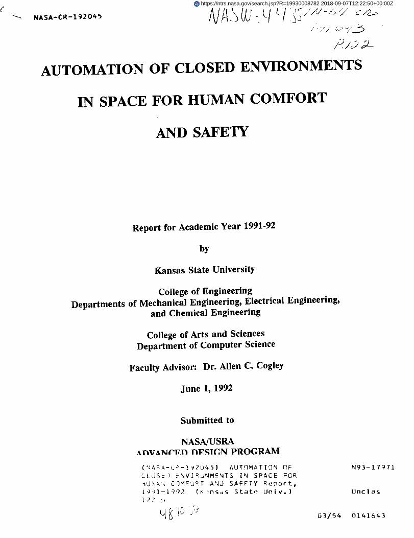
NASA-CR-192065/

/_,13 i.L

AUTOMATION OF CLOSED ENVIRONMENTS

IN SPACE FOR HUMAN COMFORT

AND SAFETY

Report for Academic Year 1991-92

by

Kansas State University

College of Engineering

Departments of Mechanical Engineering, Electrical Engineering,

and Chemical Engineering

College of Arts and Sciences

Department of Computer Science

Faculty Advisor: Dr. Allen C. Cogley

June 1, 1992

Submitted to

NASA/USRAAr_VA_r_.l_ nl_,,qlGN PROGRAM

(_JA£A-C#-I _2L)4 5) AUTOMATION OF

CL)S_) _ NVIR,_NMENTS IN SPACE FOR

1U,_',&'I C]Mr:t]c;",[ A_J SAFFTY Report,

19'_1-1g_2 (K _nsds Stat_ Univ. )

i 2 2 :)

63154

N93-t7971

Unclas

0141643

https://ntrs.nasa.gov/search.jsp?R=19930008782 2018-09-07T12:22:50+00:00Z

ABSTRACT

This report culminates the work accomplished during a three year

design project on the automation of an Environmental Control and

Life Support System (ECLSS) suitable for space travel and

colonization. The system would provide a comfortable living

environment in space that is fully functional with limited human

supervision. A completely automated ECLSS would increase astronaut

productivity while contributing to their safety and comfort. The

first section of this report, Section 1.0, briefly explains the

project, its goals, and the scheduling used by the team in meeting

these goals. Section 2.0 presents an in-depth look at each of the

component subsystems. Each subsection describes the mathematical

modeling and computer simulation used to represent that portion of

the system. The individual models have been integrated into a

complete computer simulation of the CO 2 removal process. In

Section 3.0, the two simulation control schemes are described. The

classical control approach uses traditional methods to control the

mechanical equipment. The expert control system uses fuzzy logic

and artificial intelligence to control the system. By integrating

the two control systems with the mathematical computer simulation,

the effectiveness of the two schemes can be compared. The results

are then used as proof of concept in considering new control

schemes for the entire ECLSS.Section 4.0 covers the results and

trends observed when the model was subjected to different test

situations. These results provide insight into the operating

procedures of the model and the different control schemes.The

appendix, section 5.0, contains summaries of lectures presented

during the past year, homework assignments, and the completed

source code used for the computer simulation and control system.

i

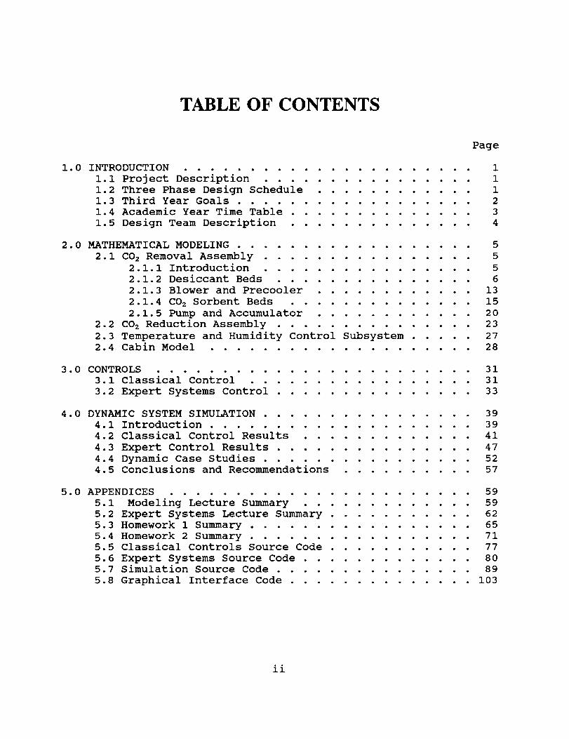
TABLE OF CONTENTS

Page

1.0 INTRODUCTION _ _ _.................. 1

i.I Project Description" . ............... 1

1.2 Three Phase Design Schedule ............ 11.3 Third Year Goals .................. 2

1.4 Academic Year Time Table .............. 3

1.5 Design Team Description .............. 4

2.0 MATHEMATICAL MODELING .................. 5

2.1 CO z Removal Assembly ................ 5

2.1.1 Introduction ................ 5

2.1.2 Desiccant Beds ............... 6

2.1.3 Blower and Precooler ............ 13

2.1.4 CO z Sorbent Beds .............. 15

2.1.5 Pump and Accumulator ............ 20

2.2 CO 2 Reduction Assembly ............... 23

2.3 Temperature and Humidity Control Subsystem ..... 272.4 Cabin Model .................... 28

3.0 CONTROLS ........................ 31

3.1 Classical Control ................. 31

3.2 Expert Systems Control ............... 33

4.0 DYNAMIC SYSTEM SIMULATION ................ 39

4.1 Introduction .................... 39

4.2 Classical Control Results ............. 41

4.3 Expert Control Results ............... 47

4.4 Dynamic Case Studies ................ 524.5 Conclusions and Recommendations .......... 57

5.0 APPENDICES ....................... 59

5.1 Modeling Lecture Summary ............. 59

5.2 Expert Systems Lecture Summary ........... 62

5.3 Homework 1 Summary ................. 65

5.4 Homework 2 Summary ................. 715.5 Classical Controls Source Code ........... 77

5.6 Expert Systems Source Code ............. 805.7 Simulation Source Code ............... 89

5.8 Graphical Interface Code .............. 103

ii

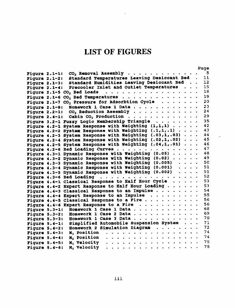
LIST OF FIGURES

PageFigure 2.1-1= CO 2 Removal Assembly ............. 5

Figure 2.1-2= Standard Temperatures Leaving Desiccant Bed . ii

Figure 2.1-3: Standard Humidities Leaving Desiccant Bed . . 12

Figure 2.1-4: Precooler Inlet and Outlet Temperatures . . . 15

Figure 2.1-5 CO 2 Bed Loads • 18

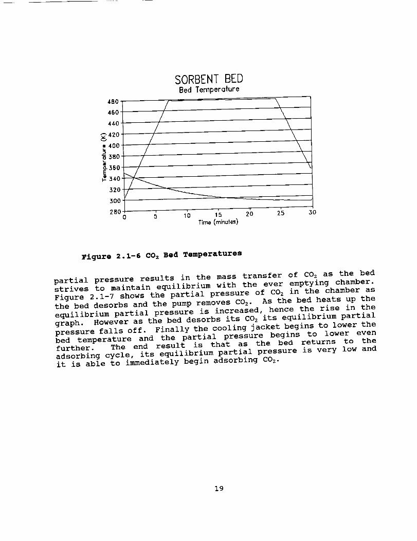
Figure 2.1-6 CO 2 Bed Temperatures .............. 19

Figure 2.1-7 CO2 Pressure for Adsorbtion Cycle ....... 20

Figure 2.1-8: Homework 1 Case 1 Data ............ 23

Figure 2.2-1: CO2 Reduction Assembly ............ 24

Figure 2.4-1: Cabin CO 2 Production ............. 29

Figure 3.2-1 Fuzzy Logic Membership Triangle 35

I_eeumeeFigure 4.2-1 System Response with Weighting (1,1 1) ..... 42

Figure 4.2-2 System Response with Weighting (.i,1,.1) .... 43

Figure 4.2-3 System Response with Weighting (.03,1,.03) . . . 44

Figure 4.2-4 System Response with Weighting (.02,1,.02) . . 45

Figure 4.2-5 System Response with Weighting (.04,1,.01) . . . 46

Figure 4.2-6 Bed Loading Curves ............... 47

Figure 4.3-1 Dynamic Response with Weighting (0.05) ..... 48

Figure 4.3-2 Dynamic Response with Weighting (0.02) ..... 49

Figure 4.3-3 Dynamic Response with Weighting (0.005) .... 50

Figure 4.3-4 Dynamic Response with Weighting (0.001) .... 51

Figure 4.3-5 Dynamic Response with Weighting (0.002) . . . 51

Figure 4.3-6 Bed Loading .................. 52

Figure 4.4-1 Classical Response to Half Hour Cycle ..... 53

Figure 4.4-2 Expert Response to Half Hour Loading ...... 53

Figure 4.4-3 Classical Response to an Impulse ........ 54

Figure 4.4-4 Expert Response to an Impulse ......... 55

Figure 4.4-5 Classical Response to a Fire .......... 56

Figure 4.4-6 Expert Response to a Fire ......... 56

Figure 5.3-1: Homework 1 Case 1 Data ............ 58Figure 5.3-2:

Figure 5.3-3:

Figure 5.4-1:

Figure 5.4-2:

Figure 5.4-3:

Figure 5.4-4: M 2 Position

Figure 5.4-5: M I Velocity

Figure 5.4-6: M 2 Velocity

Homework 1 Case 2 Data ............

Homework i Case 3 Data ............

Simplified Automobile suspension System . . .

Homework 2 Simulation Diagram .......

M I Position .................

69

70

71

72

74

74

75

75

iii

1.0 INTRODUCTION

1.1 Project Description

For prolonged missions into space and colonization outside the

earth's atmosphere, development of Environmental Control and Life

Support Systems (ECLSS) are essential to provide astronauts with

habitable environments. ECLS systems for Space Station Freedom

(SSF) require semi-autonomous operation to allow environmental

control without constant supervision by crew members. The Kansas

State University Advanced Design Team is in the process of

researching and designing a control system for an ECLSS like that

on Space Station Freedom.

The ECLS system for Freedom is composed of six subsystems. The

Temperature and Humidity Control (THC) subsystem maintains the

cabin temperature and humidity at comfortable levels. The

Atmosphere Control and Supply (ACS) subsystem insures proper cabin

pressure and partial pressures of oxygen and nitrogen. To protect

the space station from fire damage, the Fire Detection and

Suppression (FDS) subsystem provides fire sensing alarms and

extinguishers. The Waste Management (WM) subsystem compacts solid

wastes for return to earth, and collects urine for water recovery.

Carbon dioxide and other dangerous contaminants are removed from

the air by the Atmosphere Revitalization (AR) subsystem. The Water

Recovery and Management (WRM) subsystem collects and filters

condensate from the cabin to replenish potable water supplies, and

processes urine and other waste waters to replenish hygiene water

supplies.

At this time, automation and control of these subsystems have not

been fully developed or integrated. A fully integrated and

automated ECLS system would increase an astronaut's scientific and

observational productivity as well as contribute to their safety

and comfort.

1.2 Three Phase Design Schedule

Kansas State University implemented a three phase approach to

facilitate the design of a control scheme for an ECLS system. Each

phase, consisting of one academic year, represented an evolution

and advancement of previous progress.

The first phase consisted of information gathering and determining

the particular tasks required for design of the ECLS system. This

1

accumulated knowledge led to the present organizational structurecentered on six interconnected subsystems.

The second phase examined the Air Revitalization subsystem. Theconcept of a series of mathematical models providing input to acontrol system was chosen. Prototype models of the CO 2 Removal

Assembly governed by a crude expert system controller were

developed.

The third phase concentrated on refining the CO 2 Removal Assembly

and comparing two control schemes. The two control systems

compared are a classical proportional-integral-differential

controller and an expert system fuzzy logic controller. The

purpose of this study is to enhance the knowledge of these control

approaches so choices can be made for the control scheme for the

entire ECLS system.

1.3 Third Year Goals

Initially, the proposed goals for the third phase of the design

project were to combine the control systems of the six subsystems

and form an overall control system for ECLSS with fault diagnosis.

However, due to lack of control systems for the individual

subsystems, the goals for phase three were reevaluated.

The overall objective of the final year is to develop and compare

expert and classical systems of control on a computer simulation of

the CO 2 Removal Assembly of the ECLSS.

Goals for reaching the final objective begin with creating a

mathematical model and a computer simulation of the CO 2 Removal

Assembly. Concurrently, development of the classical and expert

systems of control were performed. The next goal is to integrate

the control systems and the computer simulation together and

evaluate and compare the effectiveness of each control system. The

comparison will be used as a proof of concept to evaluate the use

of expert systems to control the entire ECLSS.

A list of the goals for the third and final year are as follows:

i. Complete the computer simulation of the CO 2 Removal Assembly.

2. Create a set of rules for the expert control system of the

C02 Removal Assembly.

3. Create a classical controls system for the CO 2 Removal

Assembly.

•

.

Establish a means of communication between the mathematical

model and the two controls systems.

Analyze the dynamic response of the simulation and compare the

two methods of control.

1.4 Academic Year Time Table

The year started with an introduction to the advanced design teams

objectives for the project. Several lectures given by faculty and

graduate members of Kansas State University introduced the design

team to mathematical modeling, simulation and control. This

introduction lasted until September 25 th.

The next step was to plan objectives for the first semester, and

decide what should be .accomplished for the third year. A

comparison of expert system controls and classical system controls

for a subassembly of the ECLSS was decided upon as the third year

main objective.

Three modeling groups and two controls groups were formed to

develop models for the individual parts of the CO 2 Removal

Assembly. The modeling of the desiccant beds, the blower/

precooler, and the CO z sorbent beds began about October 23 rd, with

completion deadlines planned for November i0 _. These models were

to be integrated together forming a computer simulation of the

overall process• A presentation of the progress was given onNovember 25 th.

Documentation of the semesters work started on December 2nd and a

semester report was submitted to the faculty advisors on January23 rd"

The final semester goals were to refine the math models formulated

during the fall semester, complete implementation of controls on

the CO 2 Removal System, and create a user interface using X

Windows.

On January 30 th two modeling groups were formed. One to refine the

math model of the sorbent beds and another to find information on

the inputs and outputs to the CO 2 Removal Assembly. Two other

groups were formed to implement class/_cal and expert controls on

the CO 2 Removal Assembly. On March 4--, work on a Graphical User

Interface (GUI) using X Windows was begun. All phases were

completed for the All University Open House on April 4 th with

displays in the College Engineering and the College on Arts &

Sciences.

Documentation and a presentation for the USRA/NASA Design Program

was begun on April 6t"and continued until the day of the conference

on June 15 th.

1.5 Design Team Description

The Advanced Design Team at Kansas State University is composed of

students from several academic disciplines. Currently

participating disciplines include computer science, and mechanical

engineering and chemical engineering. The team's Graduate Teaching

Assistant is an electrical engineer. Plans are under way to

recruit students from electrical and computer engineering for the

final semester. Faculty support comes from the mechanical,

electrical, chemical, and computer engineering departments as well

as the computer science department.

2.0 MATHEMATICAL MODELING

2.1 CO2 Removal Assembly

2.1.1 Introduction

The Carbon Dioxide Removal Assembly, designed to remove carbon

dioxide from the cabin air, involves removal of CO 2 by molecular

sieves. The process is required to remove carbon dioxide generated

by the respiratory processes of the astronauts and to maintain

acceptable levels of carbon dioxide within the cabin.

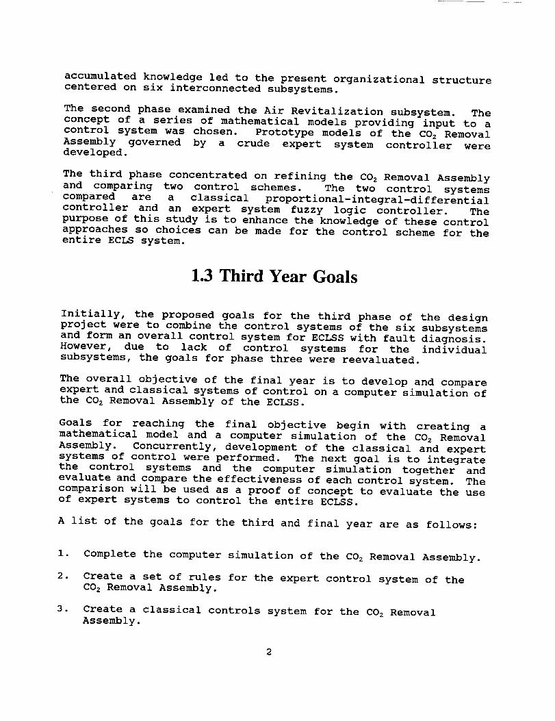
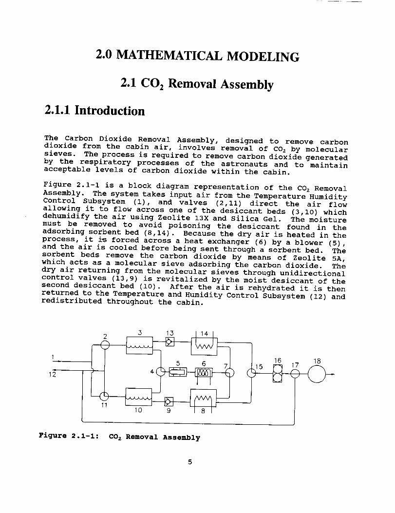
Figure 2.1-1 is a block diagram representation of the CO 2 Removal

Assembly. The system takes input air from the Temperature Humidity

Control Subsystem (i), and valves (2,11) direct the air flow

allowing it to flow across one of the desiccant beds (3,10) which

dehumidify the air using Zeolite 13X and Silica Gel. The moisture

must be removed to avoid poisoning the desiccant found in the

adsorbing sorbent bed (8,14). Because the dry air is heated in the

process, it i_ forced across a heat exchanger (6) by a blower (5),

and the air is cooled before being sent through a sorbent bed. The

sorbent beds remove the carbon dioxide by means of Zeolite 5A,

which acts as a molecular sieve adsorbing the carbon dioxide. The

dry air returning from the molecular sieves through unidirectional

control valves (13,9) is revitalized by the moist desiccant of the

second desiccant bed (i0). After the air is rehydrated it is then

returned to the Temperature and Humidity Control Subsystem (12) and

redistributed throughout the cabin.

I

3 13 I 14 I

11 ' 10 ' _ I I 8 I'

16 18

Figure 2.1-i: C02 Removal Assembly

5

Concurrently, a second desorbing sorbent bed (14) is being heatedcausing the separation of the carbon dioxide from the desiccant.The desorbed carbon dioxide is drawn from the bed by means of apump (16) and is sent to an accumulator tank (18). After theadsorbing desiccants have become saturated, the desorbing beds areonce again dry. The control valves (5,7,15) redirect air flow inthe system. The previously adsorbing beds begin the desorbingprocess and the previously desorbing beds begin adsorbing. Thesystem is presently configured to cycle every thirty minutes.

Mathematical models of the various components were created to allowanalysis of the subassembly's performance. The role of themodeling is to duplicate the actual systems response to a given setof parameters• Knowing how an actual system should respond, it ispossible to explore control systems for use in governing thesubassembly. The control systems regulate the state variablesthroughout the subassembly.

2.1.2 Desiccant Beds

DESCRIPTION

The purpose of the desiccant beds is to remove water vapor from the

incoming air. This function is necessary because water will poison

the zeolite used in the CO 2 adsorption process• Water vapor

removal is achieved by means of two desiccants, Silica gel and

Zeolite 13X. High-humidity air coming into the CO 2 Removal

Assembly flows first over the Silica gel, which removes some of the

water and brings the relative humidity down to a low level. Since

Zeolite 13X works well at low relative humidities, it is then used

to remove most of the remaining water vapor before the air is sent

on to the blower and precooler. The exiting air is not only dry,

but also heated from the release of energy required to condense the

water vapor• As adsorption is taking place in one bed, the other

desiccant bed is rehumidifying the air returned from the CO 2

sorbent beds through a desorption process• The desorbing cycle is

just the reverse of adsorbing in that hot, dry air flows across the

Zeolite 13X first, then over the Silica gel, and is cooled and

humidified in the process•

MATH MODEL

Assumptions

i • Equilibrium relative humidity is a linear function of load for

Silica gel, while that for Zeolite 13X can be approximated

with two straight lines.

6

2. All heat transfer is between the air and water only.

3. Water in the desiccant is evenly distributed at all times.

4. Beds remain at room temperature•

5. Air is heated before desorption.

6. The water is removed and released at constant pressure.

7. The specific heat of the air is constant.

• Enthalpy of condensation and vapor saturation pressure are

accurately represented by linear and fourth order least

squares curve fits, respectively.

9. Equilibrium relative humidity, which is a function only of the

load on the desiccant bed, is achieved•

Equations

A thermodynamic analysis of the air flowing through the bed yields

the following equations used for the mathematical model• Equation

1 is a curve fit for vapor saturation pressure as a function of

saturation temperature. Values for the curve fit were obtained

from the steam tables in an appendix of Thermodynamics, An

Enqineerinq Approach by Cengel and Boles. The expression is

Psat=.3972+.O629T+.OOlO99_+l.705x10-s_+6.192x10-v2 _. (i)

From the same text, relationships equating pressures, mass, and

relative and absolute humidities are shown in equations 2, 3, and

4 as

Pv=_Psa:, (2)

.622P v_: (3)

P-Pv '

_mf (4)mY" 1 +_

The law of mass conservation can be applied to the model when

evaluating the air inside the desiccant bed. The mass of dry air

in the bed (m,) equals the total mass of air in the bed (mr) minus

the mass of water vapor in the air (my) state as

ma=m_-m v. (5)

The load on the desiccant can be defined as the mass of water vaporabsorbed versus the mass of desiccant in the bed expressed as

L- roads • (6)

m tank

Equilibrium load curves were provided by Dr. Byron Jones of Kansas

State University from an ASHRAE reference. Data points taken from

these curves of the load versus relative humidity for the

desiccants were curve fit using a least squares method fortran

program written by Dr. Kirby Chapman, professor of Mechanical

Engineering at Kansas State University. The resulting linear curve

fits are given in Equations 7, 8, and 9. The fit for Zeolite 13X

was approximated using the two straight lines of equations 8 and 9.The results are

¢= L (Silica gel), (7).5263

_=.4L (Lg.17, Zeolite 13X), (s)

_=.068+40(L-.17) (L>.I7, Zeolite 13X) . (9)

The mass of water removed from the air can be determined using the

thermodynamic relationship

mz=mv-_m a . (I0)

Enthalpy, the incoming air temperature, and the outgoing air

temperature are related by the thermodynamic reations

h_=2502-2.389_n, (ii)

and

m_h:g (12 )T2=Tin+ (mf-m r) cp"

The remaining equations are simply relationships for the rates of

mass absorbed or desorbed, and the change in mass of air vapor and

air in the bed versus time. These equations govern the masstransfer of the water from the desiccant and the air. Utilized in

a finite time step process, the following expressions determine the

success of the desiccants in removing water from the air.

d__md, _ d__mm (13 )

d__t dt

dm dm-----v ----T

d_tt d t

(14)

dm: _ dm r

dt dt(15)

The symbols used in the mathematical model are defined as follows.

Psat

T

Pv

P

mf

m,L

mads

mt_

mr

h_8

Tin

Tz

Cp

dmads

dt

dmr

dt

dmv

dt

dm_

dt

= vapor saturation pressure (kPa)

= temperature of air being evaluated (°C)

= partial pressure of the water vapor (kPa)

= relative humidity

= absolute humidity

= total pressure of the air (kPa)

= mass of vapor in the air (kg)

= total mass of air in the bed (kg)

= mass of dry air in the bed (kg)

= load on the desiccant

= mass of water adsorbed by the desiccant (kg)

= mass of desiccant material (kg)

= mass of water removed from the air (kg)

= enthalpy of condensation (kJ/kg)

= temperature of incoming air (K)

= temperature of outgoing air (K)

= specific heat of air (kJ/kg.K)

= rate at which the desiccant adsorbs water (kg/s)

= rate at which water is removed from the air (kg/s)

= change in mass of vapor in the air (kg)

= change in total mass of air in the bed (kg)

MODELING TECHNIQUES

A computer program was written to simulate the performance of thedesiccant beds in time. This was accomplished by choosing a small

time step, and then evaluating the above equations for the mass in

the bed during that time step. The first calculations on this mass

9

determine the composition of the air based on the input conditions.Next, the equilibrium relative humidity is found from the load onthe first desiccant to come in contact with the air flow -- Silicagel for adsorbing, Zeolite 13X if desorbing. The change in theamount of water in the air is found from the difference between theinput and equilibrium states, with removal of water from the airconsidered positive. The temperature change of the air isdependent on the amount of water removed. However, changing thetemperature of the air also alters its relative humidity (but notthe absolute humidity) so that it no longer matches equilibrium.Therefore, an iterative procedure is required to find the pointwhere the output temperature and its corresponding humidities areconsistent with the equilibrium relative humidity and the newamount of water in the air. Execution of the program showed thatan average of five iterations were needed. With this done, themass of air is sent on to the other desiccant, and the calculationsare repeated to produce the final output conditions of the air fromthe bed.

It should be noted that little distinction is made between theadsorbing and desorbing cycles. This is because the desiccantitself is unaware of the intended function; it merely reachesequilibrium with the conditions it is given. Naturally, adsorptionwill occur when cool, humid air passes over desiccant with a lowloading. In order for the loaded desiccant to be desorbed by thedry air on the return trip, the air must first be heated by meansof a heat exchanger because hotter air holds more water vapor.Since the current system does not account for heating the air, theprogram sets the input temperature to a sufficiently high value onthe desorption cycle.

RESULTS

Many simulations were run with the program, each time varying one

parameter to observe its effect. Since the temperature and

relative humidity of the air being sent to the CO 2 desorption

process (and then back to the cabin) are the most important, it is

no surprise that they have the greatest effect on the performance

of the desiccant beds. Temperature is the most influential of all

parameters because relative humidity is a function of temperature.

The mass of the desiccant is also an important parameter, since it

affects the loading. Ideally, any problems with the amount of

absorbed water vapor could be solved by varying the desiccant masswithin the bed.

The following are expected normal operating conditions, inputs, and

experimentally determined values:

Mass flow rate of air

Adsorption input temperature

.2 kg/s300 K

I0

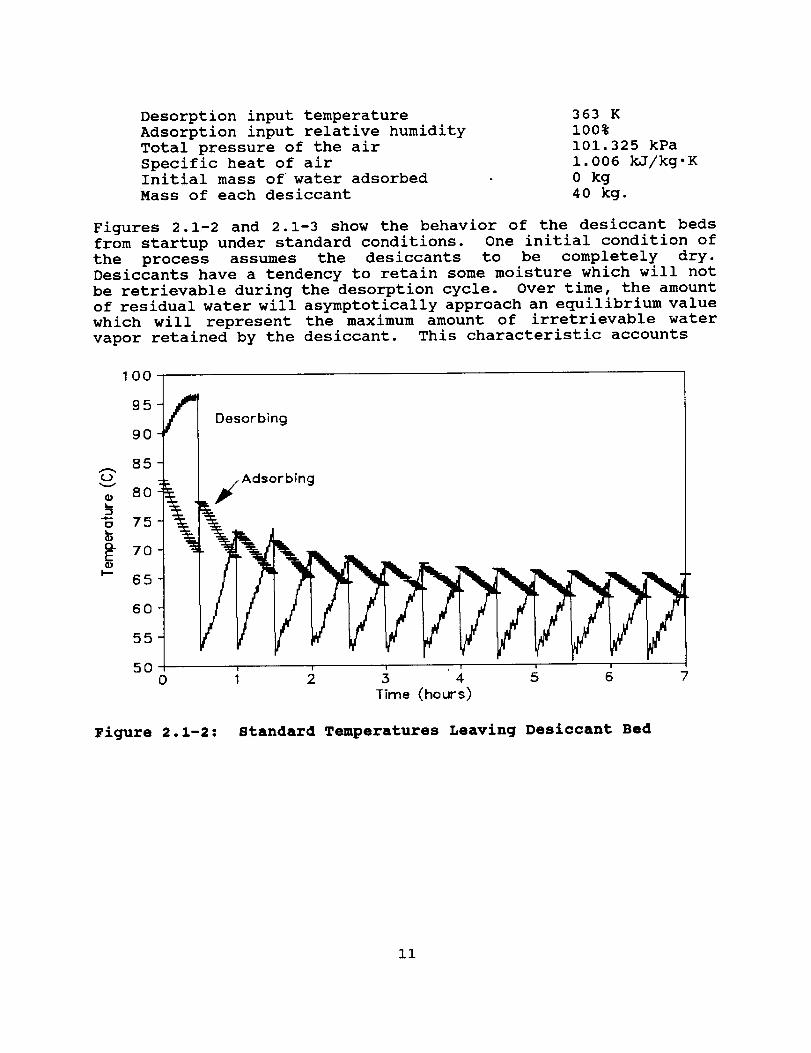
Desorption input temperatureAdsorption input relative humidityTotal pressure of the airSpecific heat of airInitial mass of water adsorbedMass of each desiccant

363 K100%101.325 kPa1.006 kJ/kg.K0 kg40 kg.

Figures 2.1-2 and 2.1-3 show the behavior of the desiccant bedsfrom startup under standard conditions. One initial condition ofthe process assumes the desiccants to be completely dry.Desiccants have a tendency to retain some moisture which will notbe retrievable during the desorption cycle. Over time, the amountof residual water will asymptotically approach an equilibrium valuewhich will represent the maximum amount of irretrievable watervapor retained by the desiccant. This characteristic accounts

100

95

9O

85

75

7O65

6O

55

5O

/_ Desorbing

Time (hours)

Figure 2.1-2: Standard Temperatures Leaving Desiccant Bed

ii

0.3

0.250

E

"_ 0.2mo

°m

0.15

Desorbing

\ \

i I!

\

\J\

%

\\\\

\ \ \\ ' \

\mm

0.1

0.05

___o 1 _ i _ 5 o 7Time (hours)

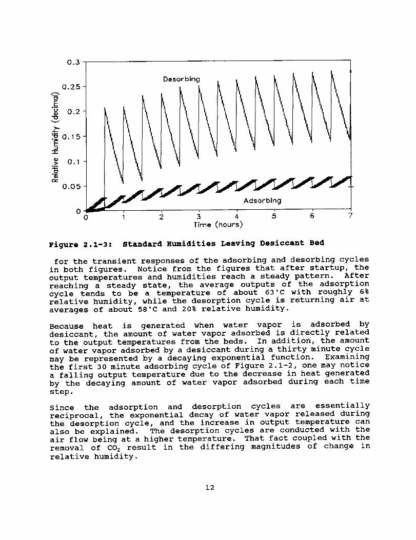
Figure 2.1-3: Standard Humidities Leaving Desiccant Bed

for the transient responses of the adsorbing and desorbing cycles

in both figures. Notice from the figures that after startup, the

output temperatures and humidities reach a steady pattern. After

reaching a steady state, the average outputs of the adsorption

cycle tends to be a temperature of about 63°C with roughly 6%

relative humidity, while the desorption cycle is returning air at

averages of about 58°C and 20% relative humidity.

Because heat is generated when water vapor is adsorbed by

desiccant, the amount of water vapor adsorbed is directly related

to the output temperatures from the beds. In addition, the amount

of water vapor adsorbed by a desiccant during a thirty minute cycle

may be represented by a decaying exponential function. Examining

the first 30 minute adsorbing cycle of Figure 2.1-2, one may notice

a falling output temperature due to the decrease in heat generated

by the decaying amount of water vapor adsorbed during each time

step.

Since the adsorption and desorption cycles are essentially

reciprocal, the exponential decay of water vapor released during

the desorption cycle, and the increase in output temperature can

also be explained. The desorption cycles are conducted with the

air flow being at a higher temperature. That fact coupled with the

removal of COz result in the differing magnitudes of change in

relative humidity.

12

2.1.3 Blower and Precooler

DESCRIPTION

The blower/precooler is the second process of the CO 2 Removal

Assembly. This process utilizes a variable speed blower to force

cabin air through the CO 2 Removal Assembly and a crossflow heat

exchanger to cool air received from the desiccant beds. Air

leaving the precooler is then directed on to the sorbent beds wherecarbon dioxide is removed.

MATH MODEL

Assumptions

i. Pressure drop across the cooler is negligible.

2. Water specific heat and air density are constant properties.

Specification of Heat Exchanqer

i. Heat exchanger effectiveness is 0.80.

2. Heat exchanger coolant is water.

3. Mass flow of coolant is 3.79 kg/min (500 ibm/hr.).

4. Inlet temperature of coolant is 15°C (59°F).

5. Cross-sectional area is 11.1 m 2 (120 FT2).

Equations

Equation 1 is the maximum heat transfer rate that can be drawn from

the air by the heat exchanger. Equation 2 is the actual heat

transfer rate using the heat exchanger effectiveness. The concepts

give

Q_.x (t) =C M (T (t)-T c ) (I)--p,air--air _h,i -- ,i l

Qact(_t)--Eg .x(_t). (2)

13

Equation 3 is the temperature of the air leaving the precooler as

a function of time given the inlet temperature, the actual heat

transfer rate and the mass and specific heat of air. Symbolically

this can be written as

T_h,ou(t_) i(t)-Qa0 ( )

C air_M ir--p,

(3)

The inlet temperature function used to test the program is given as

T--h.i(t) :2t+T_ . (4)

This function varies with time because the outlet temperature from

the desiccant beds is not constant. Note .that the equation used

does not represent the actual desiccant bed outlet temperature, but

is only an approximate linear function used to test the response of

the precooler model at extreme conditions.

The symbols used in the above equations are defined as follows:

Cp, air

E

Mair

Qact (t)

Qm_ (t)

Tc,i

= specific heat of air (kJ/kg.K),

= heat exchanger effectiveness,= mass flow rate of air into cooler (kg/s),

= actual heat transfer between two fluids (kW),

= maximum amount of heat transfer between two fluids,

(hot inlet air and cold coolant water) (kW),

= inlet temperature of cooling water (K),

Th,i(t ) = inlet temperature of hot air (K),

Th,out(t) = outlet temperature of cooled air (K),

To = initial temperature of inlet air (300 K),

t = time (minutes).

RESULTS

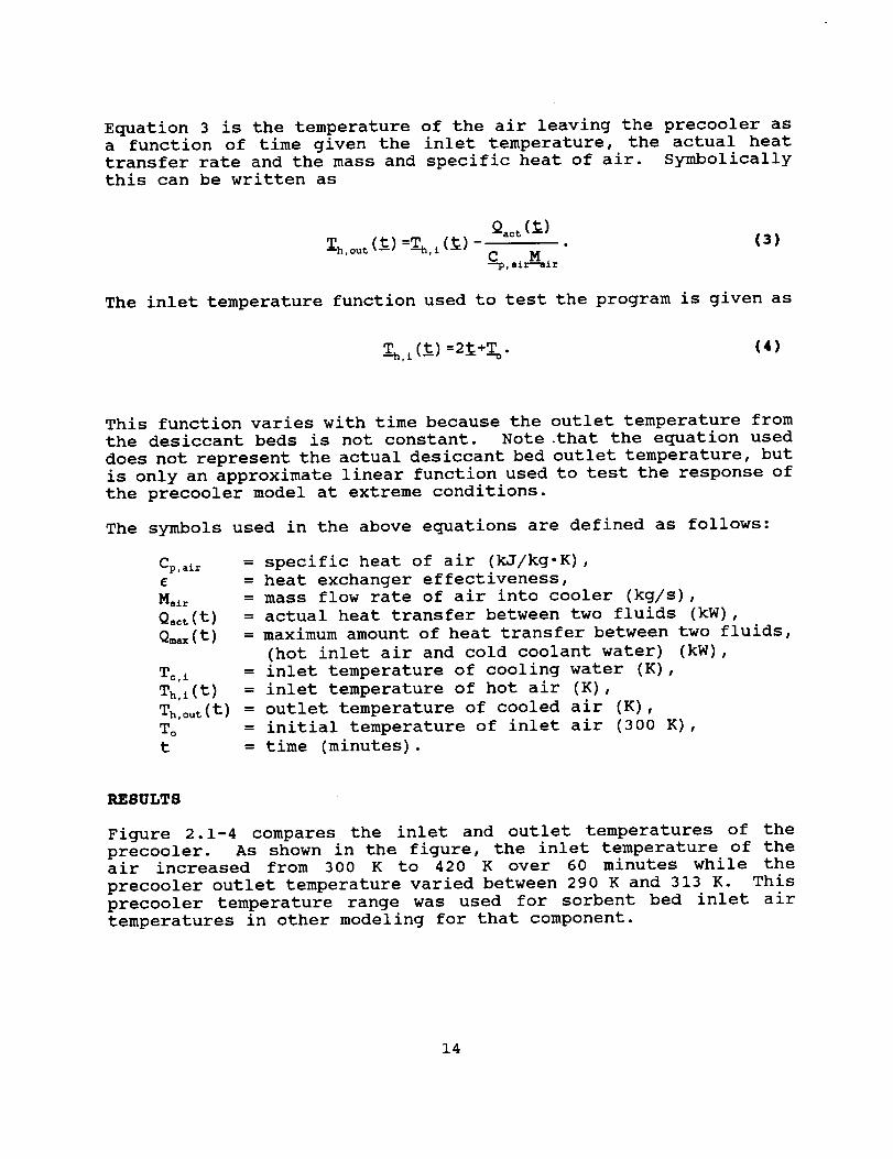
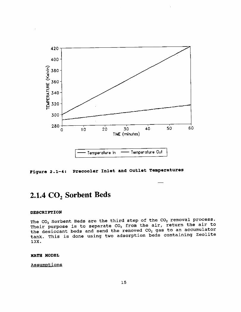
Figure 2.1-4 compares the inlet and outlet temperatures of the

precooler. As shown in the figure, the inlet temperature of theair increased from 300 K to 420 K over 60 minutes while the

precooler outlet temperature varied between 290 K and 313 K. This

precooler temperature range was used for sorbent bed inlet air

temperatures in other modeling for that component•

14

420

4OO

C•_ 38O

w 360

< 340LtJQ."_ 320,,iI--

300

280 2'o 3_ _ 5'0TIME (minutes)

6O

-- Temperoture In -- Tempera|ure Ou|

Figure 2.1-4: Preoooler Inlet and Outlet Temperatures

2.1.4 CO2 Sorbent Beds

DESCRIPTION

The CO 2 Sorbent Beds are the third step of the CO 2 removal process.

Their purpose is to separate C02 from the air, return the air to

the desiccant beds and send the removed CO 2 gas to an accumulator

tank. This is done using two adsorption beds containing Zeolite13X.

MATH MODEL

Assumptions

15

. The exiting air temperature equals the temperature of CO 2 in

the bed.

• The heat transfer coefficient of Zeolite 5A is a linear

function of temperature.

, Power supplied to the beds is either on (i000 J/s), off (0

J/s), or being removed at i000 J/s.

. Thermal equilibrium for the sorbent beds negates dependence on

bed length.

. Assume that a four man loading supplies CO 2 at an average rate

of 5.046x 10 -4 kg/s (this can be a function of time)•

Equations

The mass of CO 2 contained within an adsorbing bed at a time T is

equal to the mass adsorbed at some time T-t plus the mass

transferred during time t. The result is of the form given in

Equation 1 below. This mass transfer is brought about by the

sorbent bed removing the CO 2 based on a difference in the

equilibrium and actual partial pressures. This mass transfer is

given by equation 2 shown below• The expressions are

mT:mT_t+m_,_ t, (i)

and

rh_- (Pco2-Pequilibrium) V_ank (2 )

R co2 T tank

The ideal gas law applied in the above equations provide a simple

relationship between the mass flow rates that are desired and the

partial pressures which are known.

The energy involved in the mass transfer and accompanying phase

change results in the bed temperature being raised• In addition,

during the desorbing phase the bed is heated to drive off the CO 2

and this results in a further increase in bed temperature. This

temperature change is governed by the following energy balance:

HEAT

Tbea.°.= rbedol_4 mairCVair+ mco2CVco2 + (mbed+ mabs) CVbe d(3)

Finally, the equilibrium partial pressure curve was derived from

curve fitting data provided from Marshall Space Flight Center.

16

This data shows that the equilibrium partial pressure of the bedand air flow is a function of both the corresponding temperaturesand most importantly the bed loading, or current level of absorbedmass. This information is expressed as

PPC02=.1333 exp (I01°ad-3.065+.02622 Tbed-4.684E-5*T_). (4)

The symbols used in the above equations are defined as follows:

Tb.d = temperature of sorbent bed (K),

_02 = mass of CO 2 transferred (kg),

Pc0z = partial pressure of CO 2 (kPa),

P._il = equilibrium CO 2 concentration of bed (kPa),

Rc02 = CO 2 gas constant (kPa m3)_(kg K),

Vb, d = volume of sorbent bed (m)

HEAT = power applied to bed (J/s),

mair = mass of air in bed (kg),

mb, d = mass of sorbent bed (kg),

m_, = mass of CO 2 absorbed in bed,

cv,i r = specific heat of air (J/kg K),

CVc02 = specific heat of CO 2 (J/kg K),

cvb. a = specific heat of sorbent bed (J/kg K).

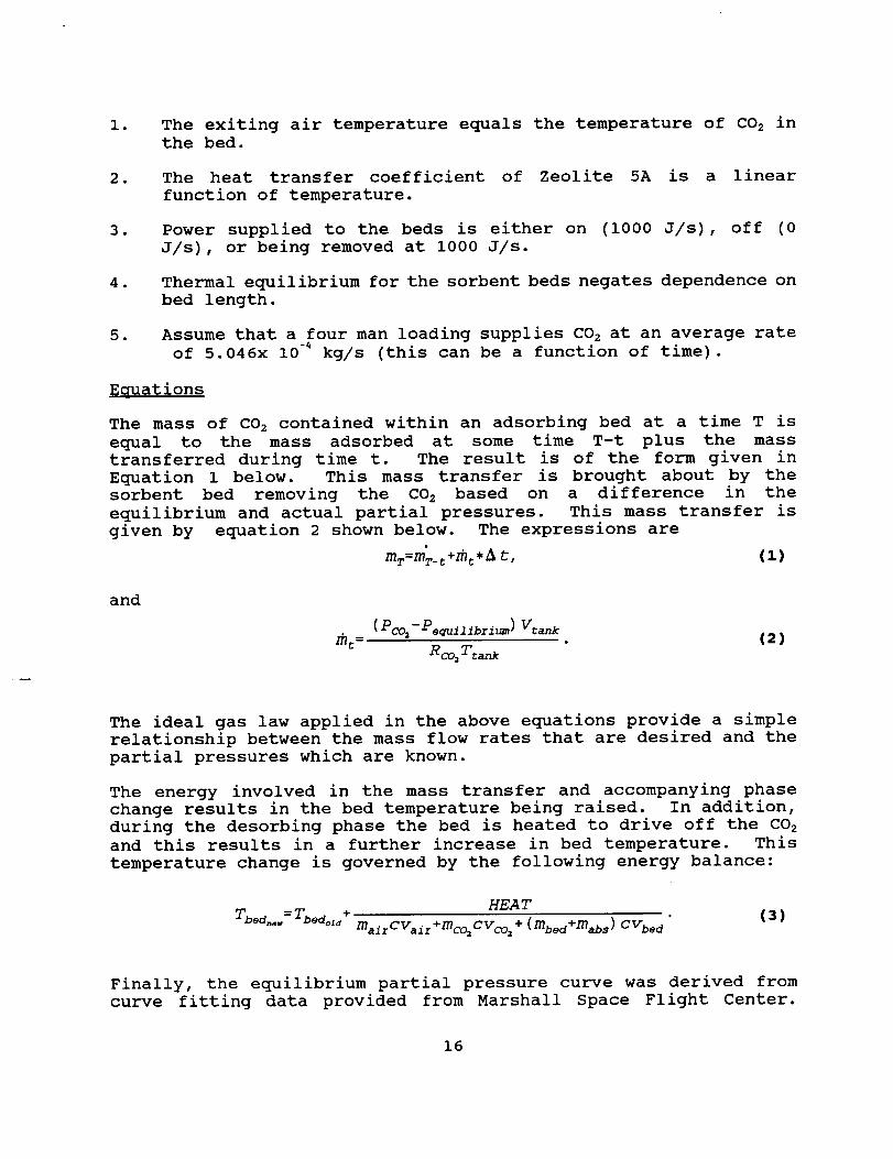
RESULTS

The system is designed to include two sorbent beds which alternate

between the adsorbing and desorbing roles. While one bed is

adsorbing the CO 2 flowing through the system, the other is being

heated and its previously adsorbed CO 2 is released and pumped out

to the accumulator tank. The Figure 2.1-5 shows the loading curves

for the two beds. The increasing curve is indicative of the bed

that is loading, while the decreasing bed's loading is shown as the

curve that is falling off.

The work done on the subroutine involved a total overhaul of the

previous semester's model due to unacceptable limitations in the

earlier version's performance. This work included enhancing the

accuracy of the model's portrayal of the actual phenomena, and

increasing the subroutine's compatibility with the main program.

After the fundamental flaws were corrected, the problem of fine

tuning the desorption process was examined. Two major criteria

were established as defining the problem. First it was neccessary

to desorb all the CO 2 in the half hour cycle, and second, it was

neccessary to provide almost pure CO 2 gas to the accumulator tank

which feeds the Bosch reactor.

17

0.0055

0.005

0.002

0.0015

SORBENT BEDBed Loading (KG/KG)

o s lo 1.5 20 25 30Time (minutes)

Figure 2. i-5 COz Bed Loads

The first problem was solved by incorporating a heating/cooling

jacket to the sorbent bed. This allowed the temperature of the bedto be raised which resulted in a lower affinity for the adsorbed

CO2. The immediate problem with this was the need to cool the bed

before returning it to the adsorbing cycle. A i000 watt

heating/cooling jacket was found to be adequate to accomplish both

of these ends.

The result of this bed heating was that the CO 2 gas was desorbed

into the bed to mix with the residual air still in the tank after

the cycle switch. During the first three minutes of the adsorbing

cycle the bed is vented into the Temperature and Humidity Control

assembly to avoid contamination of the input C02 gas for the Bosch

Reactor. The final result of the heating and cooling curves can be

seen in Figure 2.1-6.

The adsorbing process is not unidirectional in that the bed

achieves an equilibrium not neccessarily in phase with the desired

result. The temperature dependency of the equilibrium partial

pressure results in a transient desorption phase in the beginning

of the adsorption cycle. The resulting change in equilibrium

18

SORBENTBEDBed Temperature

480

45O

440

420

400

380

_-350340320

3O0

28Oo _ lb ,'s 2b 2L_ 30

Time (minutes)

Figure 2.1-6 COz Bed Temperatures

partial pressure results in the mass transfer of CO z as the bed

strives to maintain equilibrium with the ever emptying chamber.

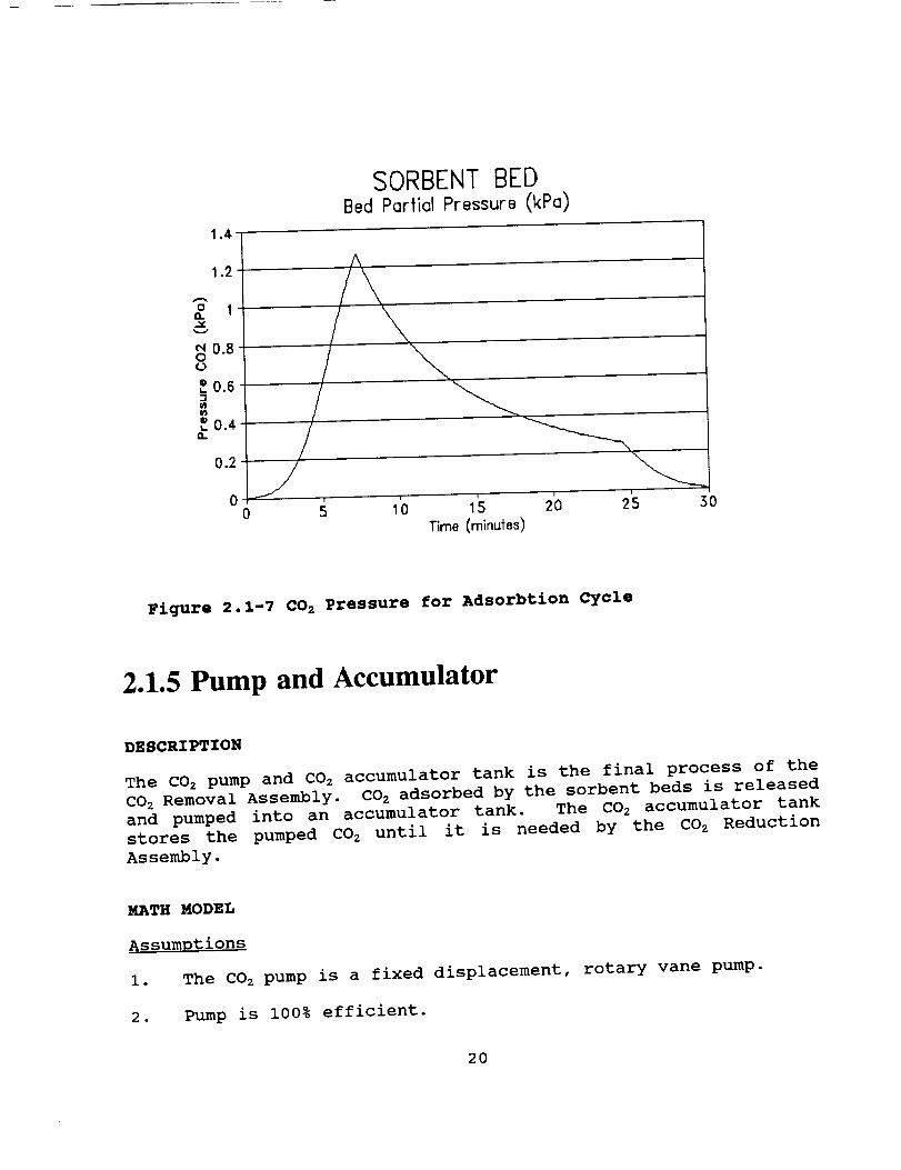
Figure 2.1-7 shows the partial pressure of C02 in the chamber as

the bed desorbs and the pump removes CO 2. As the bed heats up the

equilibrium partial pressure is increased, hence the rise in the

graph. However as the bed desorbs its CO2 its equilibrium partial

pressure falls off. Finally the cooling jacket begins to lower the

bed temperature and the partial pressure begins to lower evenfurther. The end result is that as the bed returns to the

adsorbing cycle, its equilibrium partial pressure is very low and

it is able to immediately begin adsorbing CO 2.

19

14 1

1.2

o I_u

0.8oo

_ o.s

_ 0.4

0.2 _0

0

SORBENT BEDBed Partial Pressure (kPa)

1_ 15 2'oTime (minufes)

25 30

Figure 2.1-7 COz Pressure for Adsorbtion Cycle

2.1.5 Pump and Accumulator

DESCRIPTION

The COz pump and CO 2 accumulator tank is the final process of the

CO 2 Removal Assembly. CO 2 adsorbed by the sorbent beds is released

and pumped into an accumulator tank. The C02 accumulator tank

stores the pumped CO 2 until it is needed by the CO 2 Reduction

Assembly.

MATH MODEL

Assumptions

I. The CO z pump is a fixed displacement, rotary vane pump.

2. Pump is 100% efficient.

2O

.

4.

5.

6.

Pump operates under adiabatic and isentropic conditions.

Accumulator tank is perfectly insulated.

CO 2 is an ideal gas.

CO 2 specific heat is constant.

Equations

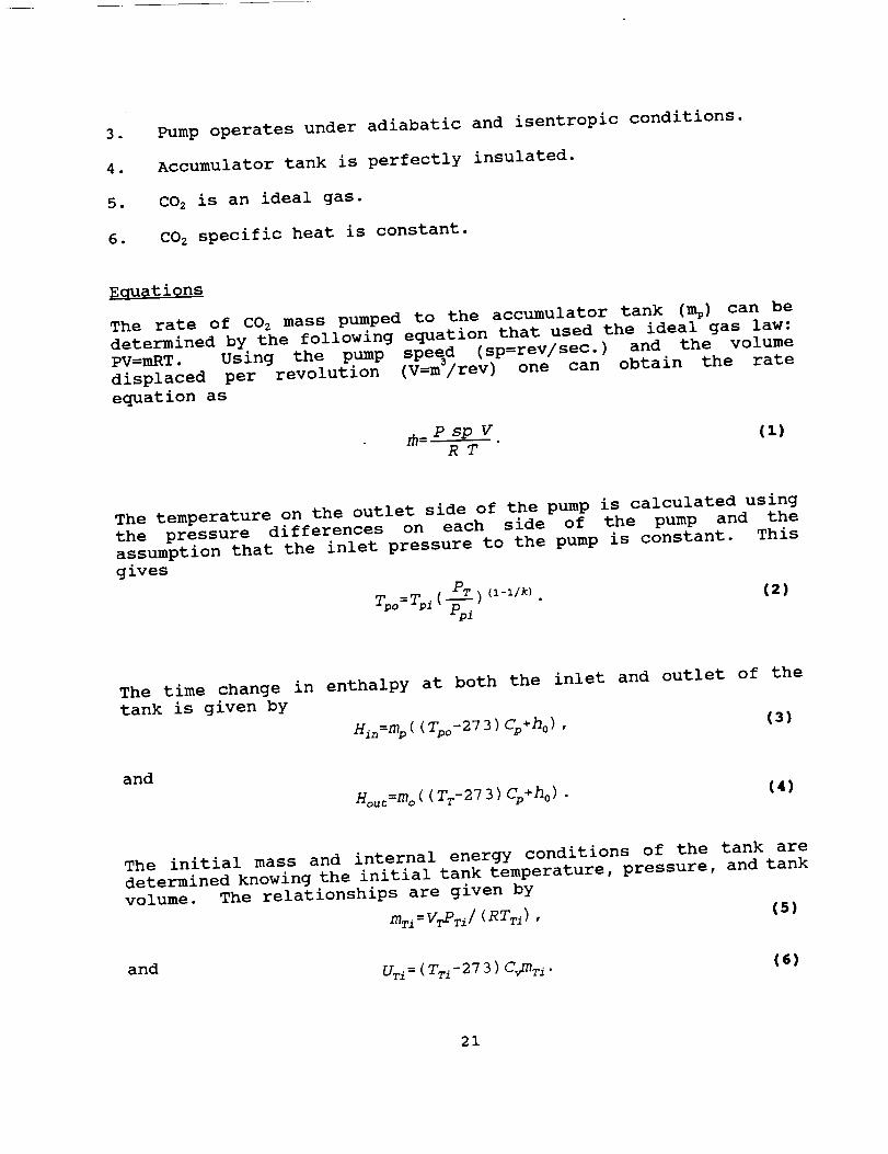
The rate of CO 2 mass pumped to the accumulator tank (mp) can be

determined by the following equation that used the ideal gas law:

PV=mRT. Using the pump speed (sp=rev/sec.) and the volume

displaced per revolution (V=m_/rev) one can obtain the rate

equation as

/n= P sp V (I)RT

The temperature on the outlet side of the pump is calculated using

the pressure differences on each side of the pump and the

assumption that the inlet pressure to the pump is constant. This

gives

PT(2)

The time change in enthalpy at both the inlet and outlet of the

tank is given by

Hin=mp ( (Tpo-27 3 ) Cp+ho> , (3)

and

Houc=lno ( (Tr-273) Cp+h o) (4)

The initial mass and internal energy conditions of the tank are

determined knowing the initial tank temperature, pressure, and tank

volume. The relationships are given by

m_ =v_Pril<_Tr_), (s)

andU'Ti= (TTi-273) Cvmri . (6)

21

The overall mass within the tank as a function of time is found by

subtracting the CO 2 drawn from the tank from the mass pumped into

the tank and adding it to initial CO 2. This can be stated as

mT=m_+ (rap-too) _s_. (7)

The current tank temperature and pressure is found using the first

law of thermodynamics and the ideal gas law respectively. These

concepts give

TT:T_+m_. iCv.co2_ / (m_2._+m r), (S )

and

Pz=mrRco2 IT� Yr. (9)

The symbols used in the mathematical model are defined as follows:

mp = mass flow rate of CO 2 from the pump (kg/sec),

sp = speed of the pump (revolutions/sec),

Vp = volume displaced by the pump per revolution (m3),

Ppi = inlet pressure to pump (kPa),

R ideal gas constant (kPa*m_/kg*K),

rpo

Tp£

P_

k

Hin

H0

Cp

Hour

mo

mzl

Vr

UTi

mz

tstp

Ur

Tz

Cv

PT

= outlet temperature of the pump (K),

= inlet temperature of the pump (K),

= pressure of CO z in the tank (kPa),

= specific heat ratio of CO2,

= enthalpy of inlet C02 stream to the accumulator (J/s),

= enthalpy of CO 2 at the reference temperature (J/kg),

= constant pressure heat capacity of CO 2 gas (J/kg*K),

= enthalpy of outlet C02 stream from accumulator (J/s),

= mass flow rate of CO 2 leaving accumulator (kg/sec),

= initial mass of CO 2 in accumulator tank (kg),

= volume of accumulator tank (m3),

= initial pressure inside tank (kPa),

= initial temperature in tank (K),

= initial internal energy of tank (J),

= current mass of CO2 in the accumulator tank (kg),

= time elapsed between calculations (sec),

= current internal energy of tank (J),

= current temperature of tank (K),

= constant volume heat capacity of CO2 (J/kg*K),

= current pressure inside tank (kPa).

RESULTS

The development of a pump and accumulator simulation was assigned

22

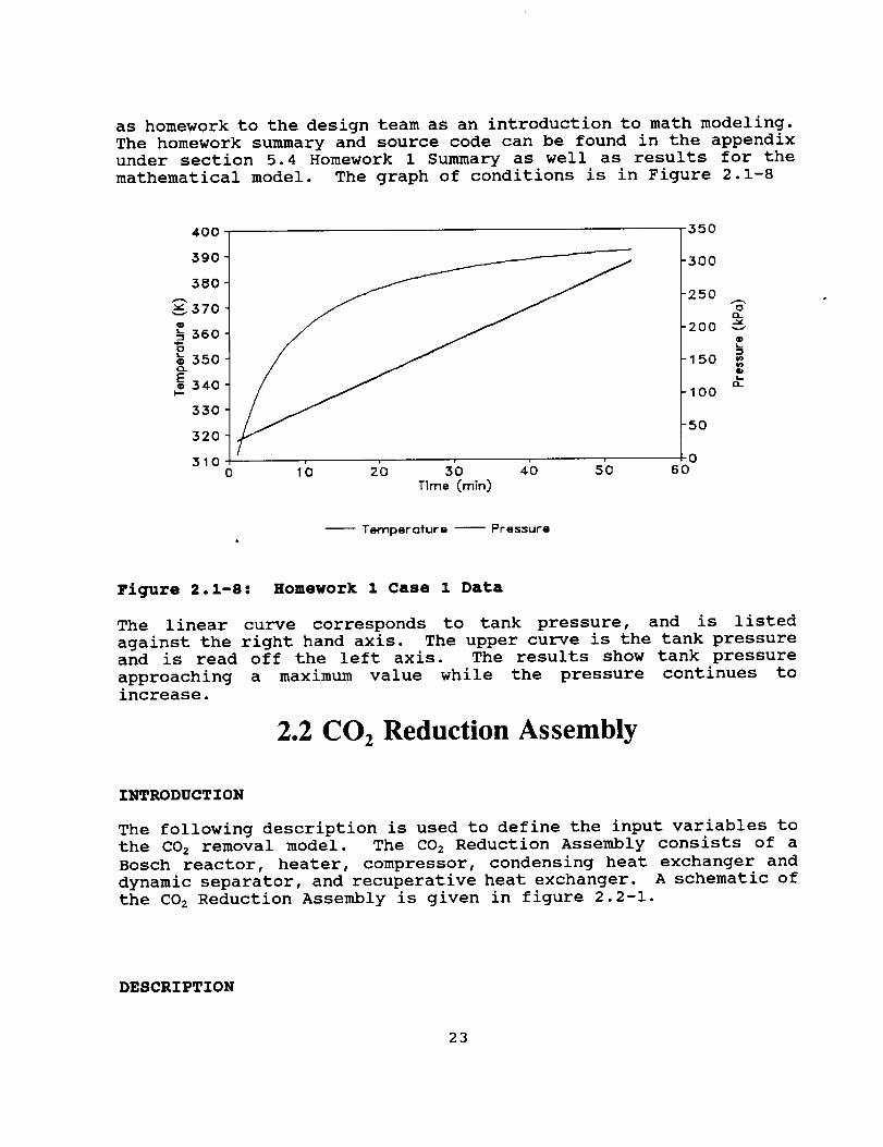
as homework to the design team as an introduction to math modeling.The homework summary and source code can be found in the appendixunder section 5.4 Homework 1 Summary as well as results for themathematical model. The graph of conditions is in Figure 2.1-8

4OO

,.'390

38O

v 370

--h3600

_ 35o

eE340I-.

33O

320

310

350

,h 2o 30 40 s'oTlme Cmin)

-300

-250

(3_

200@

150

Q

0-

-100

-50

06O

-- Tennperofura -- Pressure

Figure 2.1-8: Homework 1 Case 1 Data

The linear curve corresponds to tank pressure, and is listed

against the right hand axis. The upper curve is the tank pressureand is read off the left axis. The results show tank pressure

approaching a maximum value while the pressure continues to

increase.

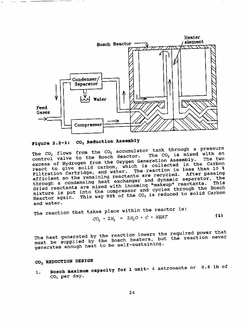
2.2 CO2 Reduction Assembly

INTRODUCTION

The following description is used to define the input variables to

the CO 2 removal model. The CO 2 Reduction Assembly consists of a

Bosch reactor, heater, compressor, condensing heat exchanger and

dynamic separator, and recuperative heat exchanger. A schematic of

the CO 2 Reduction Assembly is given in figure 2.2-1.

DESCRIPTION

23

Bosch Reactor

FeedGases

----J Condenser/_ I

Separator

/,/,//,4/,

///

/

J

/

// /_ //!\"

l'I+

Heater

p._m

. _ \\'v_.\\

Figure 2.2-1: CO2 Reduction Assembly

The C02 flows from the C02 accumulator tank through a pressure

control valve to the Bosch Reactor. The CO 2 is mixed with an

excess of Hydrogen from the Oxygen Generation Assembly. The two

react to give solid carbon, which is collected in the Carbon

Filtration Cartridge, and water. The reaction is less than I0 %efficient so the remaining reactants are recycled. After passing

through a condensing heat exchanger and dynamic separator, the

dried reactants are mixed with incoming "makeup" reactants. This

mixture is put into the compressor and cycles through the Bosch

Reactor again. This way 99% of the CO 2 is reduced to solid Carbonand water.

The reaction that takes place within the reactor is:

CO 2 + 2_ = 2H20 + C + HEAT (i)

The heat generated by the reaction lowers the required power that

must be supplied by the Bosch heaters, but the reaction never

generates enough heat to be self-sustaining.

CO 2 REDUCTION DESIGN

I. Bosch maximum capacity for 1 unit- 4 astronauts orCO 2 per day.

8.8 ib of

24

2. Modes of operation of the CO 2 Assembly

•

a. Normal mode- The Bosch is reducing CO z to water &

Carbon(S). The single pass efficiency is less than 10%, so

the reactants have to be recycled and passed back through the

Bosch. Less than one percent of the exiting reactants are not

reduced to water & solid Carbon• The Bosch will operate for

90 days before servicing the Carbon Filtration Cartridge isnecessary.

b. Standby mode- Everything is powered & ready to go exceptall valves are closed and the compressor is off.

c. Shutdown mode- The heater & compressor are off and all

valves are closed• All sensors are working.

d. Purqe mode- The system is being purged with nitrogen. The

purge is drawn off through the nitrogen purge/bleed vent. The

compressor & heater are off.

e. Unpowered mode- No electrical power is applied to system.

Process startup- The process starts in the unpowered mode and

switches to the shutdown mode. The system is checked for

leaks and if none are detected the Carbon Dioxide Reduction

Assembly is purged with Nitrogen. While the Assembly is being

purged, the heaters in the Bosch are turned on and kept at a

constant 200 °F for two hours. This is to drive off any

moisture accumulated in the Bosch during servicing of the

Carbon Filtration Cartridge. After the two hours the leak

check and purge are finished and the heater temperature is

increased to 1050 °F. The compressor is started and the purge

Nitrogen is circulated around the system. When the reactor

temperature reaches 1050 °F the reactants are introduced. The

average time from leak check to normal operating mode is 12hrs.

25

Metabolic CO 2

Flow Rate,lb_day

Temperature,-F

Pressurerpsia

H 2 Feed

Flow Rate,lb_day

Temperature,-F

Pressure,psia

Product Water

Flow Rate,lb_dayTemperature,-F

Pressure,psia

Bleed

Flow Rate,lb_day

Temperature,-F

Pressure,psia

Electric Power

28 VDC,W

115 AC,W

Heat Rejection,WTo Air

To Coolant

Desiqn Point

8.8

70

18

.8O

75

30

7.20

60

3O

1.12

75

18

341

186

529

238

Ranae8.80-17.60

60-85

14.7-20

.80-1.60

75-100

14.7-30

7.20-14.40

60-90

14.7-30

1.12

65-90

14.7-20

306-606

170-3120

494-818

181-461

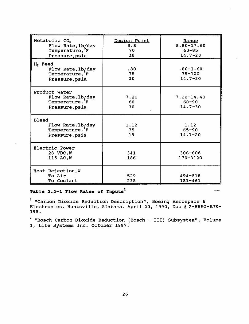
Table 2.2-1 Flow Rates of Inputs z

1"Carbon Dioxide Reduction Description", Boeing Aerospace &

Electronics. Huntsville, Alabama. April 20, 1990, Doc # 2-H8RG-RJK-

198.

2"Bosch Carbon Dioxide Reduction (Bosch -III) Subsystem", Volume

i, Life Systems Inc. October 1987.

26

2.3 Temperature and Humidity ControlSubsystem

INTRODUCTION

Because the C02 Removal Assembly model takes air from the

Temperature and Humidity Control (THC) Subsystem, it was necessary

to research the THC Subsystem and determine the effects it may have

on the air entering the CO 2 Removal Assembly.

DESCRIPTION

The principal function of the Temperature and Humidity Control

(THC) Subsystem is to maintain a comfortable environment for the

astronauts in Space Station Freedom (SSF). Air in the cabin is

continuously circulated through the THC system at 340 cubic feet

per minute. Temperature and Humidity are controlled by a

condensing heat exchanger and a slurper, respectively. Depending

on the temperature change needed to keep the cabin air within

certain specifications, a temperature control valve determines the

amount of air passed through the condensing heat exchanger. Air

not passed through the heat exchanger is bypassed to the exit side

of the heat exchanger. As air passes through the heat exchanger,

water vapor is condensed and drawn into a slurper to remove excess

water vapor in the air and prevent excessively high cabin humidity.

After leaving the heat exchanger, the air is pulled across a mixed

flow fan, and passed through an air straightener before it isreturned to the cabin.

EFFECTS ON CO z REMOVAL ASSEMBLY

According to available THC documentation, air drawn by the CO 2

Removal Assembly is taken from the THC system immediately after the

temperature control valve, and returned just before it reaches the

air straightener. This configuration is not acceptable for the

following reasons. First of all, the air drawn by the CO 2 removal

assembly cannot be taken after the temperature control valve

because in some cases, the control valve may bypass all air flow

around the heat exchanger leaving none available to the CO z Removal

Assembly. Secondly, because the air returned from the CO 2 Removal

Assembly may not be within the established cabin parameters, it

should not be returned after the THC air conditioning process.

The model will take air from the high pressure side of the THC fan

and return it to the THC Assembly at the inlet. Two assumptions

will correspond to this configuration. Because air is taken from

27

the THC after the heat exchanger, inlet conditions into the CO 2

Removal Assembly will be assumed to remain within cabin parameters.

Secondly, the flow rate of air from the CO z Removal Assembly will

be assumed much smaller than that being drawn from the cabin so the

retruned air cannot cause a false response in the temperaturecontrol valve.

CABIN PARAMETERS

The cabin pressure operates between 14.5 and 14.9 psia, and the

temperature will be kept between 65 and 80 °F. Relative humidity

and partial pressure of CO 2 will be maintain within 25 to 75 %

humidity and 3 to 12 mm of mercury, respectively.

The only cabin parameter which will act independently of the THC

system is the production of CO 2. A schedule which approximates the

production of CO 2 by the astronauts for a 24 hour period is

described in Section 2.4.

The effects of these parameters on the model will be tested within

and outside of the ranges given.

2.4 Cabin Model

DESCRIPTION

A model of the cabin was produced to simulate the effects of CO z

production and removal on the cabin atmosphere. The model

simulates temperature, pressure, and relative humidity levels

within the cabin by three different functions: a constant value,

sinusoidal and step functions varying within specified parameters.

For each time step, the model evaluates the amount of CO2 produced

within and removed from the cabin and determines the current

partial pressure of CO 2 inside the cabin.

MATH MODEL

The model allows for the cabin conditions of temperature, pressure,

and relative humidity to be simulated in several ways. Relative

humidity and temperature can be varied by use of either a sine or

step function and will fluctuate between any given parameters

establish within the program. The model also allows for varying

the cycle time of each function. Because normal cabin pressure

conditions only fluctuate between 99.9 and 102.7 kPa, the pressure

is only simulated by either a constant value or a sine function.

After the values for the cabin pressure, temperature, and relative

28

humidity are determined for a particular time step, the programevaluates the amount of COz produced by the astronauts for thattime step.

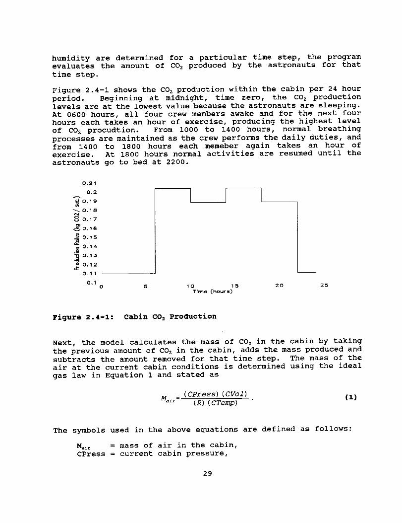
Figure 2.4-1 shows the CO2 production within the cabin per 24 hour

period. Beginning at midnight, time zero, the CO 2 production

levels are at the lowest value because the astronauts are sleeping.

At 0600 hours, all four crew members awake and for the next four

hours each takes an hour of exercise, producing the highest level

of CO 2 procudtion. From i000 to 1400 hours, normal breathing

processes are maintained as the crew performs the daily duties, andfrom 1400 to 1800 hours each memeber again takes an hour of

exercise. At 1800 hours normal activities are resumed until the

astronauts go to bed at 2200.

O.21

0.2

0.19

S o.1"1._,z 0.16

._ 0.1,5o

._ 0,14.

._ 0.13

A._ 0,12

0.11

0.10 5 10 15 20 2,.5

TTme (hours)

Figure 2.4-1: cabin COz Produotion

Next, the model calculates the mass of CO z in the cabin by taking

the previous amount of CO 2 in the cabin, adds the mass produced and

subtracts the amount removed for that time step. The mass of the

air at the current cabin conditions is determined using the ideal

gas law in Equation 1 and stated as

(CPress) (CVol )

Mair = (R) (CTemlD)(1)

The symbols used in the above equations are defined as follows:

Malr = mass of air in the cabin,

CPress = current cabin pressure,

29

CVolRCTemp

= cabin volume (i01.i15 m_),= gas constant (8.314/29),

= current cabin temperature (°C).

The mole numbers for the cabin air and the CO 2 in the cabin are

calcuated by dividing the mass of the air and CO 2 by the molecular

mass of air and C02, respectively. Next, the mole fraction of CO 2

to air is calculated by dividing the number of CO z moles by the

number of moles of air, and the paritial pressure is calculated by

multiplying the current cabin pressure by the mole fraction. The

caculated cabin partial pressure of CO 2 is then checked to

determine if the CO 2 removal assembly needs to be turned on to

remove any excess CO 2.

3O

3.0 CONTROLS

3.1 Classical Control

DESCRIPTION

The CO 2 removal sub-assembly is responsible for maintaining the

partial pressure of CO 2 with in normal limits as the astronauts and

other equipment and experiments produce it. NASA grades air

quality by the partial pressure of COz, with normal CO 2 pressure

being 0.0667 kPa. When the CO 2 partial pressure is above 0.4 kPa

the air is classified as "degraded" and above 1.015 kPa the

condition is classified as "emergency". The CO 2 removal sub-

assembly removes CO 2 from the cabin environment and stores it as a

gas in a CO 2 accumulator tank until the Bosch reactor breaks it

down to solid carbon and water.

The CO 2 removal sub-assembly uses a variable speed fan to force air

through the system's beds, ducts and heat-exchangers. The

desiccant beds and the CO 2 sorbent beds operate on 30 minute

cycles, where one bed adsorbs mass for 30 minutes while the

companion bed is desorbing. After 30 minutes the beds reverse

roles and the full adsorbing bed desorbs its mass while the empty

desorbing bed adsorbs mass.

CLASSICAL CONTROLS

There are two inputs that control the operation of the CO 2 removal

sub-assembly, the partial pressure of CO 2 in the cabin and the

pressure of CO 2 in the CO z accumulator tank. The cabin CO 2 pressure

input is used as input to a classical control to maintain the cabin

CO 2 pressure. If the partial pressure of C02 in the cabin deviates

from the desired 0.0667 kPa the system would modify the air flow

rate.

The input from the CO 2 accumulator tank was based on the gas

pressure in the tank. The Bosch reactor is an important producer

of fresh water and a shortage of COz may mean a corresponding

shortage of fresh water. The Bosch reactor shuts down if the

pressure of the supply CO 2 (the CO 2 tank) dips below 101.125 kPa,

so the system is turned on if the pressure in the CO 2 accumulator

tank drops below 137 kPa. This safety buffer of 36 kPa assures

that the tank pressure should not go below the lower limit of

101.125 kPa.

Internal to the CO 2 removal sub-assembly are controls that maintain

31

the pressure of the CO z accumulator tank and a valve that is

positioned before the CO 2 accumulator tank and after the CO z pump

that controls the purity of the CO 2 entering the tank.

The cabin air is driven through the system by a variable speed,

zero-inertia fan that is controlled to maintain cabin pressure of

0.0667 kPa. Classical control of the fan speed is accomplished by

using a proportional-integral-differential (PID) compensator in a

negative feedback loop. The PID compensator uses an error function

6, defined as the difference between the actual CO z cabin pressure

and the desired cabin pressure. The magnitude of the change in the

pump speed is given as

+ d6+f6dt. (i)

The fan speed is then adjusted by this amount, increasing or

decreasing the tank pressure.

The valve between the CO 2 accumulator tank and the CO 2 pump serves

two purposes. One is to direct CO 2 gas to the accumulator tank when

the pressure in the desorbing CO 2 sorbent bed is within 1% of the

equilibrium pressure of CO 2 for the bed. This insures that the gas

that is directed to the CO 2 tank is almost entirely CO 2. The other

purpose is to quickly evacuate the air from the CO 2 sorbent bed

that just switched to the desorbing cycle. As the beds switch, the

full bed that is just beginning to desorb contains cabin air and

CO 2 trapped in the absorbent material. For the first several

minutes of the desorbing cycle the gas removed from the bed is air

and, as the pressure in the bed decreases as the air is removed,

the temperature of the bed increases and the equilibrium pressure

of the CO 2 trapped in the Zeolite begins to increase. As the

pressure of the bed and the CO 2 equilibrium pressure converge, the

purity of the CO 2 gas leaving the bed increases. When there is a

difference of greater than 1% between the pressures, the valve

directs the gas back to the exit gas from the adsorbing CO 2 sorbent

bed and turns the CO 2 pump to its maximum speed to expedite the

emptying of the bed.

32

3.2 Expert Systems Control

IMPLEMENTATION

The simulation of the Carbon Dioxide Removal Assembly can be

controlled by an expert system written in CLIPS using fuzzy logic.

The simulation for the physical system is written in FORTRAN. The

purpose of using FORTRAN is that an existing FORTRAN simulation has

already been developed by mechanical engineers of the NASA group.

Last semester we struggled with choosing between C and FORTRAN as

a simulation language. The simulation equations were taken from

the existing FORTRAN simulation and implemented in C. The C model

then communicated with CLIPS to make a separate model apart from

the classically controlled simulation.

Originally the computer science students felt that it would be

easier to integrate CLIPS into the C environment. Since they would

be implementing the CLIPS program into the simulation, they felt

they should work with a program that was most familiar to them,

hence C. Later on when the expert control was running, it was

found that it was a painfully slow working with the simulation.

This is caused by too much file I/O overhead. The reason for this

is that CLIPS cannot communicate or link to any programming

language other than itself. The problem is sharing variables

between two languages. On the one hand, we did not want to

implement the whole model within CLIPS. It is not that easy to

program a simulation using an expert systems programming language.

Rules do not get fired in the order that one expects. On the other

hand, we did not want to implement the whole system in C either.

Programming a recursive expert systems controller in C can be quite

a struggle. It would be easier to use an expert systems program

that was designed to do just that. Therefore, we were left with

the job of integrating the two into one environment. Initially we

used a file sequencer that monitored the reading and writing of the

variable files between C and CLIPS. This was extremely slow and

used about 90% of the processor of a Soulbourne SPARC computer

running UNIX System Release V.

Since the original design was slow and the system administrators of

the computer resources weren't happy that it took so much processor

time, we ventured to design a new system. Semaphores was one of

the solutions that were brought up, but no success on

implementation was ever achieved. A semaphore is a process that

gets "forked" off from the initial process. What a semaphore does

is protect what is known as a critical section. In our case, the

critical section is the file being passed between CLIPS and C.

This file contains all of the variables pertinent to the running of

the simulation. Some of the variables simply get read by the

processes, and other get changed in the process. However, most, if

not all, variables in this file get changed at one time or another.

33

The problem is that not both processes can be writing to this fileat the same time. This would cause chaos. So this is where asemaphore becomes useful. A semaphore would allow the C program to

start its simulation process, and when it was ready, "fork" off the

expert control CLIPS process. You then tell the semaphore where

the critical section of code exists (the reading and writing of the

variables file), and then both processes can run simultaneously

waiting for the next one to hand control to it. Again, a semaphore

in this case would keep the variable file from being written to at

the same time by two different processes. However, as stated

before, a working implementation of semaphores was never worked

out.

So then we move onto the third and final design which we are

currently using. The C simulation was dropped and the FORTRAN

simulation was used for both the expert control and the PID control

to maintain a completely consistent environment.

At this point we are in the Spring 1992 semester of implementation

of the project. We have decided to use FORTRAN as the simulation,

C and Xwindows for a user interface, CLIPS for the expert systems

controller, and FORTRAN for the PID controller. We have also

decided to use a Soulbourne SPARC UNIX workstation as our platform

of choice. Our reasons behind this are simple; it is an extremely

fast computer, it multitasks, _nd hard disk space on this system is

plentiful.

The engineers programmed the FORTRAN simulation and PID controls

while three computer scientists programmed the expert systemscontrol and the Xwindows user interface. Much of the semester was

spent by the engineers getting a working "bug free" simulation

running so the controllers could be employed. The expert systemscontroller was built within the first month and then modules were

stubbed for tests. After this, efforts were placed on getting the

user interface to work.

There is not much to the expert systems in terms of lines of code.

However, this does not mean that it does not do a lot. Some of the

expert system was designed like the PID controller because there

was really no expertise that could be used in making a decision.

Situations such as a valve require only two positions, i.e. on or

off. Other such devices require only If/Then statements, and no

fuzzy logic was used in determining what variables to change. For

the devices that can take advantage of fuzzy logic, CLIPS becomes

very powerful. Once the engine to determine membership functions

has been written, it can be used over and over to control many

different devices. All that need be added to it are one or two

lines at the beginning of the CLIPS code that describe what ranges

the variables should exist in. The engine takes care of the rest.

One such example might be as follows:

(fuzzy tank-pressure low -150 300 400),

34

(fuzzy tank-pressure(fuzzy cabin-pressure(fuzzy cabin-pressure

high 300 400 650),low -i00 .058 .075),high .058 .075 i00).

Presently, the only component within the C02 Removal Assembly whichis controllable is a variable speed fan used to draw mass throughthe sorbent beds, which remove carbon dioxide from the atmosphere•The controller monitors the Cabin CO 2 partial pressure to determine

when the pump speed should be adjusted to maintain safe CO 2 levels.

PRESSURE CONTROL BY EXPERT SYSTEM METHODS

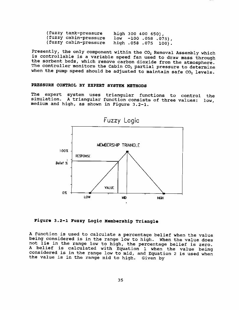
The expert system uses triangular functions to control the

simulation. A triangular function consists of three values: low,

medium and high, as shown in Figure 3.2-1.

Fuzzy Logic

100_

Belief %

0%

_EMFIERSNIP TRIANGLE

RESPONSE /

LOW MD HIG_

Figure 3.2-1 Fuzzy Logic Membership Triangle

A function is used to calculate a percentage belief when the value

being considered is in the range low to high. When the value does

not lie in the range low to high, the percentage belief is zero.

A belief is calculated with Equation 1 when the value being

considered is in the range low to mid, and Equation 2 is used when

the value is in the range mid to high. Given by

35

value-low

mid-low, (1)

and

high-value

high -mid(2)

The percentage belief is used to directly determine the amount of

change that must be made. This expert system uses two triangles to

control the simulation. The left triangle represents the low

pressure function. The right triangle represents the high pressure

function. There is also overlap between the high and low

triangles. This is not uncommon in fuzzy logic. The intersection

point of the two triangles is chosen to correspond to the target

control value and to a 50% belief in both triangles. This is done

so that when the system variable deviates from the target value,

the belief is immediately greater than 50% in one of the triangles

which prompts the system to try to correct it. The slope of both

triangles is adjusted to control the rate at which the expert

system changes the simulation. Pump speed, pump duration, and

pressure deviation are factors used in determining the adjustments

to the triangular functions. The pressure can be controlled more

accurately when the pump speed is changed more often. However,this can cause wear on a pump and must be taken into consideration.

The definition of the functions in CLIPS are as follows.

(deffacts start

(state open)

(fuzzy temp low 0 258 338)

(fuzzy temp high 268 348 600))

When the percentage belief in a low pressure is greater than 50%,

Equation 3 is used to adjust the pump speed. Likewise, when the

percentage belief of a high pressure is greater than 50%, Equation

4 is used to change the pump speed. In this way the expert system

is able to control pump speed by monitoring the tank pressure asgiven by

NewPumpSpeed=OldPumpSpeedx(l+%beliefcold), (3)

NewPumpSpeed=OldPumpSpeedx(l-%beliefhot). (4)

After trial runs were executed using these equations, it was

decided to adopt a more fluid control equation. It employs a

normalized belief, and is less prone to overshoot and repeated

searching for the desired value. Equation 5 shows the method of

36

employing this normalized belief as .

NewPumpSpeed =Ol dPumpSpeedx (1 + (2 ×%bel i ef col d- 1 ) ) . (5 )

This improved control equation was then adopted into all fullsimulation exercises.

The expert system and simulation communicate by writing a temporary

file. The two programs work in lock step. In other words, one

program runs one cycle, then the other program runs one cycle. The

FORTRAN simulation was modified to run only one time step and then

shell out to the operating system to call CLIPS. The simulationwill have to read in variables from a file each time that it runs.

It must then save the variables to the same file after each run.

The expert system will be acting in the same way with one

exception. Instead of running continuously, the expert system will

run only once, make the necessary changes to the file variables,

and then exit; thus handing control back over the simulation

program.

37

38

4.0 DYNAMIC SYSTEM SIMULATION

4.1 Introduction

DESCRIPTION OF THE CO z REMOVAL SUB-ASSEMBLY

The objective of the CO 2 Removal Sub-Assembly is to remove carbon

dioxide from cabin air and store it in an accumulator tank for

further processing. The sub-assembly consists of nine main

components: two desiccant beds, a blower, a pre-cooler, two

sorbent beds, a CO 2 pump, a CO 2 accumulator tank, and control

schemes. The function of each sub-assembly component is

described below.

The desiccant beds dehumidify used cabin air, and humidify fresh

cabin air. This is do_e simultaneously by two desiccant beds

working together at a set operating cycle. While one bed is

removing water from used cabin air, the other bed is releasing

water to carbon dioxide free, fresh cabin air.

The blower moves the cabin air through the desiccant beds and on

to the sorbent beds. The pre-cooler cools the dry cabin air from

the desiccant beds to a uniform temperature.

The sorbent beds adsorb carbon dioxide and desorb stored carbon

dioxide. This is done simultaneously by two sorbent beds working

together at a set operating cycle. While one bed is removing

carbon dioxide from dry cabin air, the other bed is releasing

stored carbon dioxide to the CO 2 accumulator tank.

The C02 pump draws off the stored carbon dioxide from one sorbent

bed and passes it on to the accumulator tank. The CO 2

accumulator tank stores released carbon dioxide from the sorbent

beds, and passes it on to the CO 2 Reduction Sub-Assembly.

The control schemes regulate the speed of the blower based on the

information on the CO 2 level in the cabin. Two different control

methods are used. The first discussed is a classical method

using a PID approach. The second method uses an expert system

and fuzzy logic to accomplish control over the blower.

DEVELOPMENT OF THE SIMULATION PROGRAM

The objective of the simulation program is to accurately model

and control the main components of the CO 2 Reduction Sub-Assembly

over a set operating time using a Fortran code program. The

simulation program is composed of a main simulation program and

39

PRECEDI_G PAGE BLANK _OT FILMED

several subroutines that model the main sub-assembly components.

Before a main program was written, individual subroutines were

written to model each main sub-assembly component. After the

subroutines worked successfully on their own, they were

integrated together using the main program.

The function of the main program is to initialize all variables

that are common to two or more subroutines, and pass these

variables through CALL statements. By initializing most of the

variables in the main program, any changes to these variables can

be done by accessing the main program only, and not each

individual subroutine. Any variables that are common to only one

subroutine were kept localized within that subroutine. The main

program operates on a set operating cycle at a constant time

step. Currently, the operating cycle of the main program is set

at 24 hours or 84600 seconds, and the time step is set at one-

tenth of a minute or 6 seconds. The name of the main program isCOOL.FOR

The function of the subroutines is to calculate common subroutine

variable values for a given time step. By keeping all

computations within the subroutines, it is easier to locate,

assess and adjust erroneous data. The names of the subroutinesare as follows:

desiccant beds: DESSBED.FOR

blower/pre-cooler: BLOWCOOL.FORsorbent beds: SORBED.FOR

sorbent beds/CO 2 pump: SORPUMP.FORaccumulator tank: CO2TANK.FOR

Analysis of the entire CO 2 Removal Sub-Assembly reveals 4 state

variables for each main component. Given as

i) mass flow rate,

2) pressure,

3) temperature,

4) relative humidity.

These state variables are coded and localized for each subroutine

by the type of variable it is (mass, pressure, temperature,

relative humidity), which subroutine it is in (DESSBED, BLOWCOOL,

SORBED, SORPUMP, CO2TANK), and whether it is at the inlet or

outlet (in, out). For example in the DESSBED subroutine, mass

flow in is represented by M for mass, DB for desiccant bed, and

IN for inlet, yielding MDBIN. Similarly, inlet pressure and

temperature are PDBIN and TDBIN and outlet mass, pressure, and

temperature are MDBOUT, PDBOUT, and TDBOUT. Following this

pattern, the following variables were coded:

40

blower/precooler: MBPIN, PBPIN, TBPIN, MBPOUT, PBPOUT, TBPOUTsorbent beds: MSBIN, PSBIN, TSBIN, MSBOUT, PSBOUT, TSBOUTpump/tank: MPTIN, PPTIN, TPTIN, MPTOUT, PPTOUT, TPTOUT

When passing variables from one subroutine to the next, theoutlet variable for one subroutine will become the inlet variablefor the following subroutine. As a result, mass out from thedesiccant beds becomes the mass in to the blower/precooler.Consequently, the main program passes the previous outletvariables in the CALL statements, but receives them with the

inlet variables in the subroutines.

4.2 Classical Control Results

INTRODUCTION

The simulation with controls needed to be thoroughly tested.

This would result in two benefits. First it would be possible to

determine if the physics of the CO z removal process were being

correctly modelled. Second, it would allow an insight into the

abilities of both the system and the controllers to handle

various situations.

The method used of evaluating the control systems was to

determine which "weighting factor" provided the most desired

response. The major characteristic looked for in the solution

was the ability of the controller to dampen out initial

transients, and settle upon a closely bound mass flow rate and

therefore CO 2 rate. This resulted in the system being run at a

nearly constant rate which greatly reduces wear on the fan due to

cycling.

Although many tests were run, the test conditions used for the

evaluation of the controllers was a simple twin step function

with an initial offset. It was desired to maintain cabin CO 2 at

0.0667 kPa throughout the test. The initial value in the cabin

was set at 0.07 kPa. The CO 2 production rate was initially given

as 1.7-i0 -s kg/sec, indicative of resting astronauts. At four

hours into the simulation this value was increased to 7.0,10 -5

kg/sec a number representing a double sized crew performing hard' -5

work. Finally at eight hours the level was decreased to 3.0,10

kg/sec a level appropriate for the standard 4 man crew performing

typical functions.

DESCRIPTION

The classic, or PID, controller was designed around the

corrective algorithm given by

41

d

--error [mm-=-+( error dt errordt__+ ÷i ) f

kl k2 k3

(6)

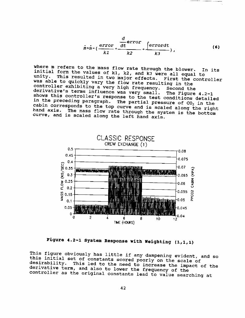
where m refers to the mass flow rate through the blower. In its

initial form the values of kl, k2, and k3 were all equal to

unity. This resulted in two major effects. First the controller

was able to quickly vary the flow rate resulting in the

controller exhibiting a very high frequency. Second the

derivative's terms influence was very small. The Figure 4.2-1

shows this controller's response to the test conditions detailed

in the preceding paragraph. The partial pressure of CO 2 in the

cabin corresponds to the top curve and is scaled along the right

hand axis. The mass flow rate through the system is the bottom

curve, and is scaled along the left hand axis.

CLASSIC RESPONSECREWEXCHANGE(I)

Figure 4.2-i System Response with Weighting (1,1,1)

This figure obviously has little if any dampening evident, and so

this initial set of constants scored poorly on the scale of

desirability. This led to the need to increase the impact of the

derivative term, and also to lower the frequency of the

controller as the original constants lead to value searching at

42

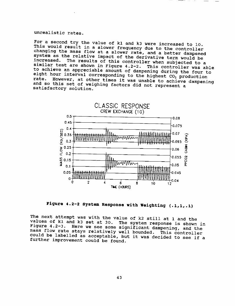
unrealistic rates.

For a second try the value of kl and k3 were increased to i0.This would result in a slower frequency due to the controllerchanging the mass flow at a slower rate, and a better dampenedsystem as the relative impact of the derivative term would beincreased. The results of this controller when subjected to a

similar test are shown in Figure 4.2-2. This controller was able

to achieve an appreciable amount of dampening during the four to

eight hour interval corresponding to the highest CO z production

rate. However, at other times it was unable to achieve dampening

and so this set of weighing factors did not represent a

satisfactory solution.

0.5

0.45

.-. 0,4oi,i

0.35

o 0.3

0.25o

0.2t,

_o.15

m 0.1

0.05

CLASSIC RESPONSECREWEXCHANGE(IO)

0.08

................._n_. AnAAAAAAnAA6_A_

FVUUUVVVVVVVWVVVVUI/IIU IIIVI/UVIIIIUItl/UIZ VUIV' _VT''ll|Ir''v'v'w*

_IIIII,14IIIIAI IIIII

IUVUVVVVVIVVVVVVVVV0 2 4

-0.075

-0.07 ,-,

o..

"0,065 ',--"_Z

-0.060

-0.05 _-

P IIUYVlIU IIVUVI .o 8 10 2

Tm_E(HOURS)

Figure 4.2-2 System Response with Weighting (.1,1,.1)

The next attempt was with the value of k2 still at 1 and the

values of kl and k3 set at 30. The system response is shown in

Figure 4.2-3. Here we see some significant dampening, and the

mass flow rate stays relatively well bounded. This controller

could be labelled as acceptable, but it was decided to see if a

further improvement could be found.

43

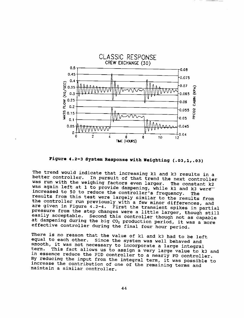
0.5

0.45

0,4O

0.35

0.3

0.25O.a 0.2'

0.15

CLASSIC RESPONSECREW EXCHANGE (30)

///I//VVVVVVV ll, tjUl/VVVVW_. - Iv V v"

.0.08

-0.075

"0.07 ,'-,

o,.

-0.065_znn

0.05 <:L.>

-0.ossoo.

-0.05 0-

o.,. AAA0.05. h ^ . . I A_AAA^^-0.045

,,VVVVVVVvvX, ....0 I I , ' I ' 0 .0 4

0 2 4. 6 8 10 12TIAE(HOURS)

Figure 4.2-3 System Response with Weighting (.03,1,.03)

The trend would indicate that increasing kl and k3 results in a

better controller. In pursuit of that trend the next controller

was run with the weighing factors even larger. The constant k2

was again left at 1 to provide dampening, while kl and k3 were--

increased to 50 to reduce the controller's frequency. The

results from this test were largely similar to the results from

the controller run previously with a few minor differences, and

are given in Figure 4.2-4. First the transient spikes in partial

pressure from the step changes were a little larger, though still

easily acceptable. Second this controller though not as capable

at dampening during the big CO 2 production period, it was a more

effective controller during the final four hour period.

There is no reason that the value of kl and k3 had to be left

equal to each other. Since the system was well behaved and

smooth, it was not necessary to incorporate a large integral

term. This fact allows us to assign a very large value to k3 and

in essence reduce the PID controller to a nearly PD controller.

By reducing the input from the integral term, it was possible to

increase the contribution of one of the remaining terms andmaintain a similar controller.

44

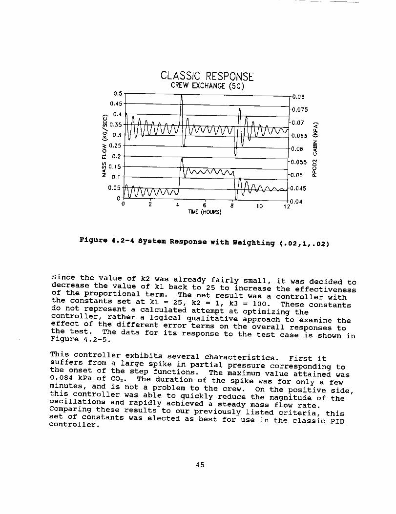
0.5

0.45

,-, 0.40

0.35

0.3

0.250" 0.2

0.15

_ 0.1

0.05

CLASSIC RESPONSECREW EXCHANGE (50)

-0.08

0 2 4 8 I06TItlE(HOURS)

-0.075

-0,07 ,-,

rt

-o.os5 _z

-O.Og <

-0.055 g

"0.05 _-

-0.045

0.042

Figure 4.2-4 System Response with Weighting (. 02, i,. 02)

Since the value of k2 was already fairly small, it was decided todecrease the value of kl back to 25 to increase the effectiveness

of the proportional term. The net result was a controller with

the constants set at kl = 25, k2 = i, k3 = i00. These constants

do not represent a calculated attempt at optimizing the

controller, rather a logical qualitative approach to examine the

effect of the different error terms on the overall responses to

the test. The data for its response to the test case is shown in

Figure 4.2-5.

This controller exhibits several characteristics. First it

suffers from a large spike in partial pressure corresponding to

the onset of the step functions. The maximum value attained was

0.084 kPa of CO 2. The duration of the spike was for only a few

minutes, and is not a problem to the crew. On the positive side,

this controller was able to quickly reduce the magnitude of the

oscillations and rapidly achieved a steady mass flow rate.

Comparing these results to our previously listed criteria, this

set of constants was elected as best for use in the classic PID

controller.

45

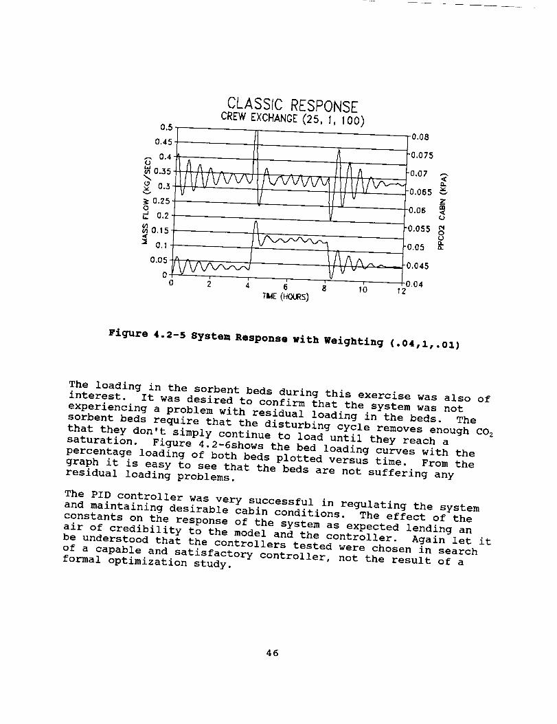
0.5

0.45

.-. 0.4o

N 0.35

0.3,,,,,W

;= 0.250"_ 0.2

(/1u_ 0.154

0.05

CLASSIC RESPONSECREW EXCHANGE (25, I, I00)

A

T_E (H_S)

0.08

-0.075

-0,07 ---,,<@.

-0.065zgB

0,05 <

"0.055 0

rl"0.05 "

0.045

0.042

Figure 4.2-5 System Response with Weighting (.04,1,.01)

The loading in the sorbent beds during this exercise was also of

interest. It was desired to confirm that the system was not

experiencing a problem with residual loading in the beds. The

sorbent beds require that the disturbing cycle removes enough CO 2

that they don't simply continue to load until they reach a

saturation. Figure 4.2-6shows the bed loading curves with the

percentage loading of both beds plotted versus time. From the

graph it is easy to see that the beds are not suffering any

residual loading problems.

The PID controller was very successful in regulating the system

and maintaining desirable cabin conditions. The effect of the

constants on the response of the system as expected lending an

air of credibility to the model and the controller. Again let it

be understood that the controllers tested were chosen in search

of a capable and satisfactory controller, not the result of a

formal optimization study.

46

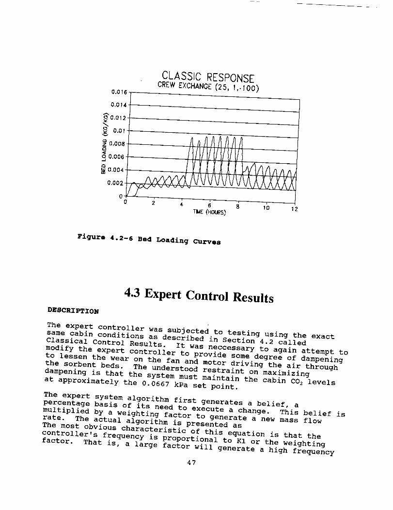
0.016

CLASSIC RESPONSECREW EXCHANGE (:25,I,-I00)

0.014

o 0.012

o 0.01v

_z°0.008E34o 0.006.,.i

a 0.00403

0.002

O0

vvvv XXX/VIIIII

I

2 4 6 8 10

TIblE(HOI.IRS)

12

Figure 4.2-6 Bed Loading Curves

4.3 Expert Control Results

DESCRIPTION

The expert controller was subjected to testing using the exact

same cabin conditions as described in Section 4.2 called

Classical Control Results. It was neccessary to again attempt to

modify the expert controller to provide some degree of dampening

to lessen the wear on the fan and motor driving the air through

the sorbent beds. The understood restraint on maximizing

dampening is that the system must maintain the cabin CO 2 levels

at approximately the 0.0667 kPa set point.

The expert system algorithm first generates a belief, a

percentage basis of its need to execute a change. This belief is

multiplied by a weighting factor to generate a new mass flow

rate. The actual algorithm is presented as

The most obvious characteristic of this equation is that the

controller's frequency is proportional to K1 or the weighting

factor. That is, a large factor will generate a high frequency

47

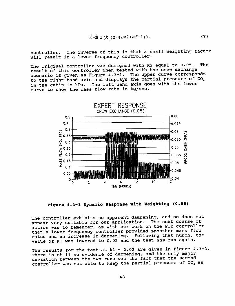
m=m +(kz(2- %Belief-l) ) . (7)

controller. The inverse of this is that a small weighting factor

will result in a lower frequency controller.

The original controller was designed with kl equal to 0.05. The

result of this controller when tested with the crew exchange

scenario is given as Figure 4.3-1. The upper curve corresponds

to the right hand axis and displays the partial pressure of C02

in the cabin in kPa. The left hand axis goes with the lower

curve to show the mass flow rate in kg/sec.

0.5

0.45

r. 0.4(2

0.55

o 0.33_

0.250

0.2L

_o._5

m 0.1

0.05

00

EXPERT RESPONSECREWEXCHANGE(0.05)

0.08

0o:o:<

Y"I?,065 v_zm

0.06 <(..)

"0.055 _>0¢L

•0.05 _-

III111tllillllll illilllillll llllig illllllli gl I

i

2 4

IIHIIIIliHI_IglUlKIIILIIIIH

/I Ill IIRII IHII Ill_

MMIIIIWl

|||||lll||alllllll|illHillgOIII@IHIIIIIiMH!IIIlITII!HlllH

6 8 10

TIIE(HOLIES)

"0.045

0.042

Figure 4.3-I Dynamic Response with Weighting (0.05)

The controller exhibits no apparent dampening, and so does not

appear very suitable for our application. The next course of

action was to remember, as with our work on the PID controller

that a lower frequency controller provided smoother mass flow

rates and an increase in dampening. Following that hunch, the

value of K1 was lowered to 0.02 and the test was run again.

The results for the test at kl = 0.02 are given in Figure 4.3-2.

There is still no evidence of dampening, and the only majordeviation between the two runs was the fact that the second

controller was not able to keep the partial pressure of CO 2 as

48

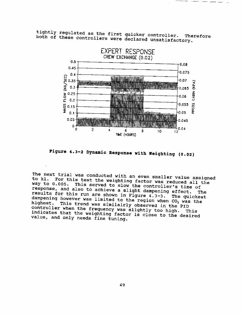
tightly regulated as the first quicker controller. Therefore

both of these controllers were declared unsatisfactory.

EXPERT RESPONSECREWEXCHANGE(0.02)

0.5

°,51 I°°80.075

,.-,, 0.4 J

lllllllAllllll_lJ-o.o_.-,(J

o.35 <

0.3 -0.065..,_ IHJllt"llllllll _z

rn0.25 I, ll,,llr,,,L,_ 0116 <o llIWlilllliltl o" 0.2" tllllllllll -o.osso"

= °" WHII[III ' ,,llr,,lfrtl

0 , 0.040 2 2

IW[JJJlt_IIIJL................................

r!tli!lllt!ftl'"II1_111111111_MIilliillIIIIIt_11_1IWfl[UllItlIH

4. 6

TI_E(HOURS)

Iilllllllllllllh,,Hl,,hm,,

lJllWl_ill_ll_ll[llllIllllilIllllIllillll_Illill_lllrl

8 10

Figure 4.3-2 Dynamic Response with Weighting (0.02)

The next trial was conducted with an even smaller value assigned

to kl. For this test the weighting factor was reduced all the

way to 0.005. This served to slow the controller's time of

response, and also to achieve a slight dampening effect. The

results for this run are shown in Figure 4.3-3. The quickest

dampening however was limited to the region when CO 2 was the

highest. This trend was similairly observed in the PID

controller when the frequency was slightly too high. This

indicates that the weighting factor is close to the desired

value, and only needs fine tuning.

49

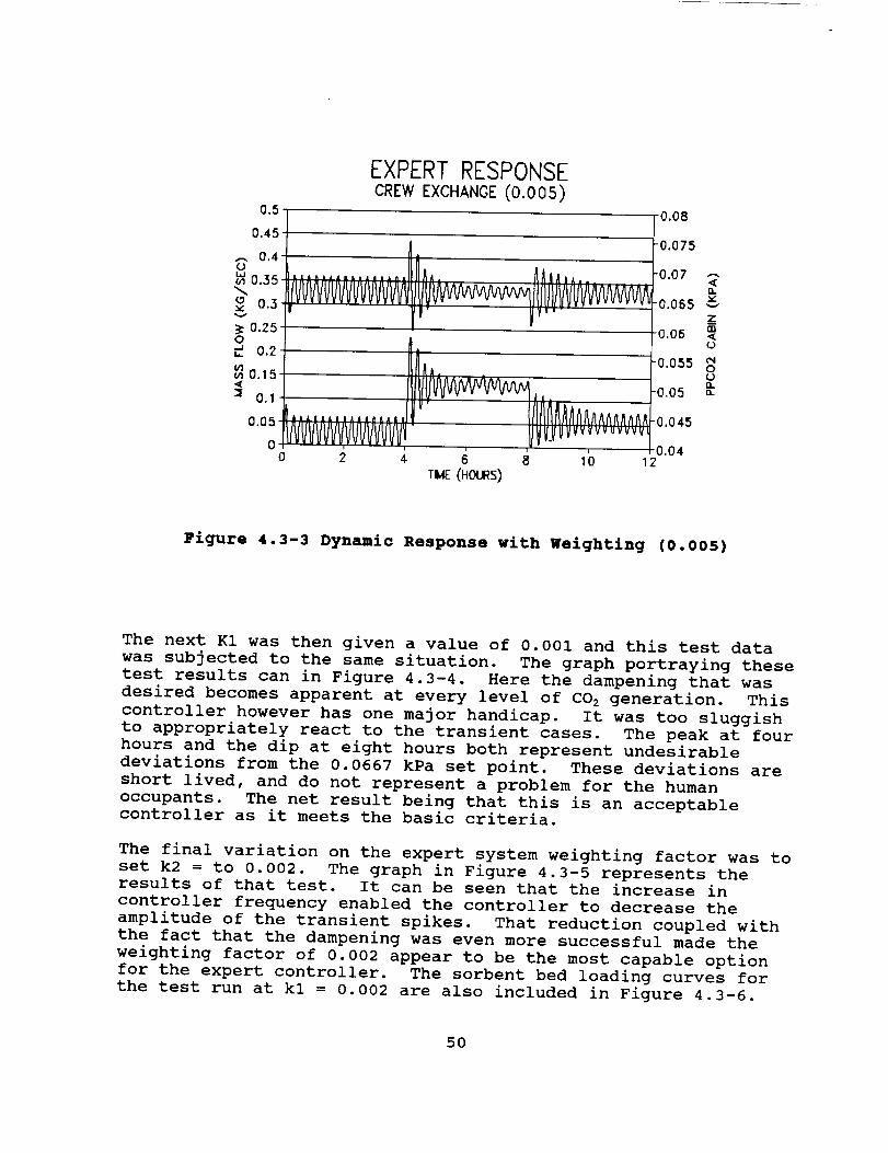
EXPERT RESPONSECREWEXCHANGE(0.005)

0.5

0.45

,,.,, 0.40

0._5

0.3

0.250

0.2 _

0.15

1_ 0.1

o vVv WvWv'ff v'viO

0 2 4.

.......Ivvvvvvv vvvvvvlvvWvvvvv

_J

TI_E(HOURS)

_/._UVvvvvvuvvvvl

-0.08

"0.075

•0.07 ,--<o.

-0.065zoo

'0.06t,,)

-o.055oOl.

-0.05 o_

-0.045

0.0410 12

Figure 4.3-3 Dynamic Response with Weighting (0.005)

The next K1 was then given a value of 0.001 and this test data

was subjected to the same situation. The graph portraying these

test results can in Figure 4.3-4. Here the dampening that was

desired becomes apparent at every level of CO 2 generation. This

controller however has one major handicap. It was too sluggish

to appropriately react to the transient cases. The peak at four

hours and the dip at eight hours both represent undesirable

deviations from the 0.0667 kPa set point. These deviations are

short lived, and do not represent a problem for the human

occupants. The net result being that this is an acceptablecontroller as it meets the basic criteria.

The final variation on the expert system weighting factor was to

set k2 = to 0.002. The graph in Figure 4.3-5 represents theresults of that test. It can be seen that the increase in

controller frequency enabled the controller to decrease the

amplitude of the transient spikes. That reduction coupled with

the fact that the dampening was even more successful made the

weighting factor of 0.002 appear to be the most capable option

for the expert controller. The sorbent bed loading curves for

the test run at kl = 0.002 are also included in Figure 4.3-6.

5O

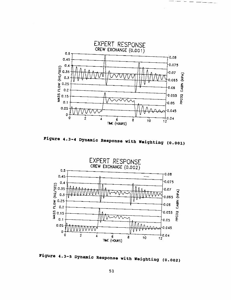
0.5

0.45

,_ 0,4<.)

0.35

0.3

_: 0.25Q" 0.2

m_0.15

"_ 0.1

0.05

00

EXPERT RESPONSECREW EXCHANGE (0.001)

"0.08

_/_ A .0.075A_.._^^. ^ ^,,.

tlIIIIJVVVXilS"vvvv_ l li llllVVV',,v VVV_

A F°'°Sso_• l l_ I-oo5_-_"

tVVVVVV_ Vv_- ], .... t 0.042 4 6 8 10 12

TIlE(HOURS)

•0.07 ."-<

i n-0.065 _v

zrr,

0.06 <o

Figure 4.3-4 Dynamic Response with Weighting (0.001)

0.5

0.45

._. 0.4o

o.s5

0.3

_: 0.250

0.2

0.15

:_ 0.1

0.05

EXPERT RESPONSECREWEXCHANGE(0.002)

0 2 ¢ 6 8 10TIIE(HOURS)

-0.08

0.075

"0.07 ,'-',.<

-0.065znn

-0.06 <{.)

0.055 _)

o..-0.05 _-

-0.045

0.042

Figure 4.3-5 Dynamic Response with Weighting (0.002)

51

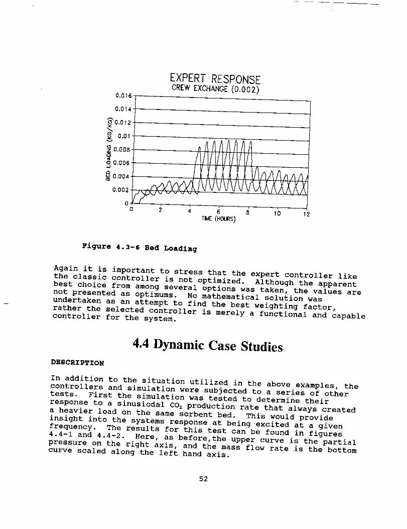
0.016

EXPERT RESPONSECREWEXCHANGE (0.002)

0.014

o 0.012'v

0.01

Oz_0,008Q

o 0.006-J

(3',' 0.004m

0.002

Oo 2 i

T_E(HOURS)

Figure 4.3-6 Bed Loadlag

Again it is important to stress that the expert controller like

the classic controller is not optimized. Although the apparent

best choice from among several options was taken, the values are

not presented as optimums. No mathematical solution was

undertaken as an attempt to find the best weighting factor,

rather the selected controller is merely a functional and capable

controller for the system.

4.4 Dynamic Case Studies

DESCRIPTION

In addition to the situation utilized in the above examples, the

controllers and simulation were subjected to a series of othertests. First the simulation was tested to determine their

response to a sinusiodal CO 2 production rate that always created

a heavier load on the same sorbent bed. This would provide

insight into the systems response at being excited at a given

frequency. The results for this test can be found in figures

4.4-1 and 4.4-2. Here, as before,the upper curve is the partial

pressure on the right axis, and the mass flow rate is the bottom

curve scaled along the left hand axis.

52

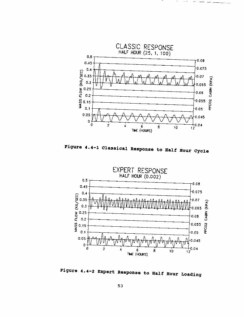
0.5

0.45

,_ 0.40

_,o.35

0.3vV

0.250-J 0.2

(n0.15

0.1

O.O5

CLASSICRESPONSEHALF HOUR (25, 1, I00)

0.08

_A

vV V

-0.075

-0.07<r_

-0.065zco

-0.06c.)

m 0 " 0 S S

(.>

' , .... J0.040 2 4 6 8 1o 12

TIIE(HOURS)

Figure 4.4-1 Classical Response to Half Hour Cycle

0.5

0.45

,-, 0.4

o.35

<s 0.5

_: 0.250•_ 0.2

_ 0.15

:_ 0.1

0.05

EXPERT RESPONSEHALFHOUR(0.002)

-0.08

-0.075

-0.07 -_-

n

-0.065 vzOB

-0.06 <(j,

o.os5L>n,

-0.05 "

-0.0450.04

0 2 4 6 8 I0 12TUE (HOURS)

Figure 4.4-2 Expert Response to Half Hour Loading

53

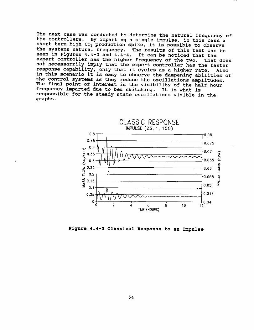
The next case was conducted to determine the natural frequency ofthe controllers. By imparting a single impulse, in this case a

short term high CO 2 production spike, it is possible to observe

the systems natural frequency. The results of this test can be

seen in Figures 4.4-3 and 4.4-4. It can be noticed that the

expert controller has the higher frequency of the two. That does

not necessarrily imply that the expert controller has the faster

response capability, only that it cycles as a higher rate. Also

in this scenario it is easy to observe the dampening abilities of

the control systems as they reduce the oscillations amplitudes.

The final point of interest is the visibility of the half hour

frequency imparted due to bed switching. It is what is

responsible for the steady state oscillations visible in the

graphs.

CLASSIC RESPONSEIMPULSE (25, 1, 100)

0.5 -0.08

0.45

,-, 0.4o

o.3s

0.3v

0.25

_, • -0.075

0.065

m•0.06 <

o

-0.055

o_-0.05

o,_1L 0.2

0.15

m 0.I

0 i ) i

0 2 4 6 8r_E (HOURS)

-0.045

0.041(3 12

Figure 4.4-3 Classical Response to an Impulse

54

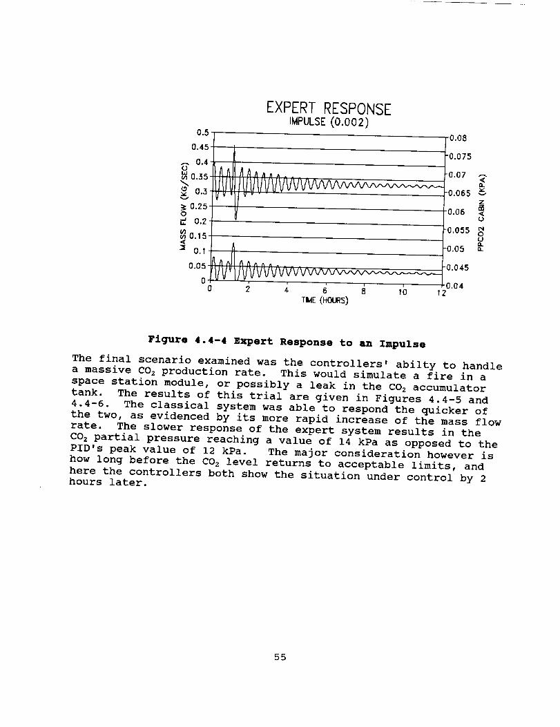
0,5-

0.45 -

.-. 0.4-0

Y,0.35-

0.3

0.25o•.J 0.'2

w 0.15

0.I

0.05

EXPERT RESPONSEIMPULSE(0.002)

-0.08

-0.075

-0.07 ,'_,<0,,v-0.065 ",-,'z_

-0.06 <0

-0.055 N0(,,)I1.

0.05 o.

0 2 4. 6 8 10 12TIIE(HOURS)

Figure 4.4-4 Expert Response to an Impulse

The final scenario examined was the controllers' abilty to handle

a massive CO 2 production rate. This would simulate a fire in a

space station module, or possibly a leak in the CO 2 accumulator

tank. The results of this trial are given in Figures 4.4-5 and

4.4-6. The classical system was able to respond the quicker of

the two, as evidenced by its more rapid increase of the mass flow

rate. The slower response of the expert system results in the

CO 2 partial pressure reaching a value of 14 kPa as opposed to the

PID's peak value of 12 kPa. The major consideration however is

how long before the CO 2 level returns to acceptable limits, and

here the controllers both show the situation under control by 2

hours later.

55

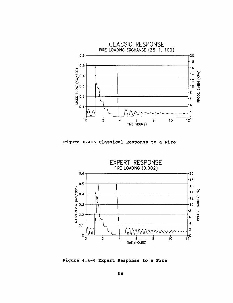
0.6

0.5<I)I,i

_0.4<.9

0.30

_=

m 0.2(/1.<[

0.1

@0 ,

0

CLASSIC RESPONSEFIRELOADING EXCHANGE (25, I, I00)

-20

-18

-16

:14v

-12 "*

10

0

I1_

-4

-20

2 4 6 8 10 12TIIE(HOURS)

Figure 4.4-5 Classical Response to a Fire

0.6

0.5

ot_

_0,4

_: 0.30...JL,,,.

m 0.2_q

0.1

%00

EXPERT RESPONSEFIRELOADING(0.002)

i

2 4 6 8 10TIlE (HOURS)

i i i

-20

18

8

"5

14

12

02

16

14 n_

12zii1

10 <

(N

0

o.I1.

Figure 4.4-6 Expert Response to a Fire

56

4.5 Conclusions and Recommendations

CONCLUSIONS

The first conclusion that can be gathered from this report is

that the simulation presented is a success. The physical

phenomena modeled are accurate and respond correctly to parameter

changes. This implies that the simulation is capable of being

used as a test bed for evaluating almost any parameter's

influence on the systems behavior. It is possible to determine

the effects of the possible disasters (such as a fire), or to

merely examine how the system operates under normal conditions.

Both controllers were found to be capable of handling the tasks

assigned. There is currently no way to evaluate the controllers

as far as superior capability. Neither was formally optimized,

and so the limit of their abilities is still not known.

RECOMMENDATIONS

It is recommended that a formal optimization of the controllers

be done. Once optimization is completed, a rigid and weighted

set of criteria should be drafted. After testing the controls

with the simulation code, the control schemes could be scored

against the criteria. Once this is completed, the better control

system should be implemented as the control scheme of choice.

Note that a single type of control may not necessarily be the

best choice. Rather, a control heirarchy where an expert system

oversees a series of classical controls (or vice versa) might bethe most effective choice.

57

58

5.0 APPENDICES

5.1 Modeling Lecture Summary

Dr. Byron Jones, professor of mechanical engineering at Kansas

State University, introduced the design team students to the

concepts of mathematical modeling and controls. The following isan outline of the lecture.

A. Definitions

i. Parameters. Parameters which are inherent to the system or

which are determined from outside the system. Parameters do not

change state variables but will affect how rate variables relate tostate variables.

2. Inputs. Inputs are variables which change state variables.The values of Rate Variables are determined from outside the

system.

3. System Relationships. The relationships that describe how the

values of the rate variables are determined from the state

variables. (This is the tough part.)

4. State Variables. Those variables required to define the state

of a system. Specifying all of the state variables completely

defines the state of a dynamic system. State variables do not

change instantaneously.

5. Rate Variables. Rate variables are those which change state

variables. The values of rate variables are determined by statevariables•

B. Dynamic Systems Simulation

Development of a set of equations (or other model) that

describes how a system behaves over time in response to various

inputs to the system.

C. Dynamics Systems Analysis

Use of various techniques to study the dynamic behavior of a

system (stability, speed of response, etc...)

De System of Equations

37

PREGEDING P_GE EILAr_I{ r_OT FILMED

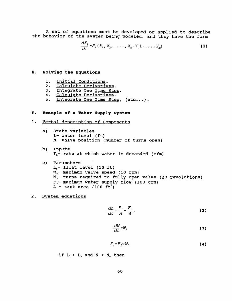
A set of equations must be developed or applied to describe

the behavior of the system being modeled, and they have the form

dX I

dt -FI(XI"X2"....'Xn"Y I, ...,Ym) (_)

E. Solving the Equations

.

2.

3.

4.

5.

Initial Conditions.

Calculate Derivatives.

Inteqrate One Time Step.Calculate Derivatives.

Inteqrate One Time Step, (etc...) .

Fo

i.

•

Example of a Water Supply System

Verbal description of Components

a) State variables

L- water level (ft)

N- valve position (number of turns open)

b) Inputs

Fo- rate at which water is demanded (cfm)

c) Parameters

_- float level (i0 ft)

W m- maximum valve speed (i0 rpm)

N m- turns required to fully open valve (20 revolutions)

F.- maximum water supply flow (I00 cfm)

A - tank area (i00 f_)

System equations

dL_Fi Fo

dt A A(2)

-- Wndt

(3)

F i=F ixN.

if L < L, and N < N m then

(4)

6O

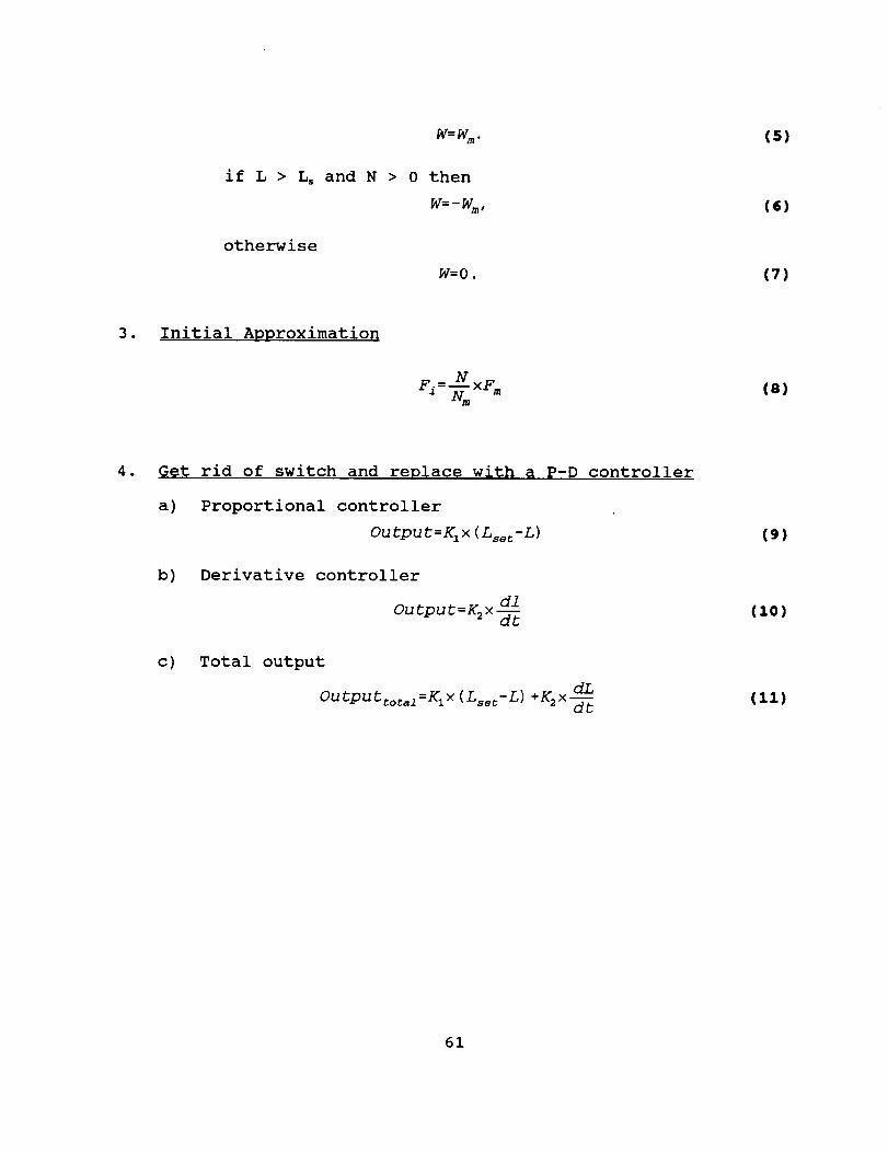
W= Wm .

if L > Ls and N > 0 then

w=-w m,

otherwise

W=0.

3. Initial Approximation

(s)

(6)

(7)

(e)

• Get rid of switch and replace with a P-D controller

a) Proportional controller

Output=K1x(Lse_-L)

b) Derivative controller

Output=_× dldt

c) Total output

Output_o_al=_X(Lse_-L)+_x-_t

(9)

(Io)

(11)

61

5.2 Expert Systems Lecture Summary

Harold Kraus, expert systems consultant at Kansas State University,

gave a two hour lecture on expert systems. Harold developed an

expert control model for the 1990-1991 NASA/USRA team. This model

was developed using CLIPS, which has highly influenced his design

and the design that is being implemented this year. The one

problem with using expert systems however in this project is that

it becomes increasingly difficult to model an Environmental Control

System when the simulation is written in FORTRAN and the expert

control is written in CLIPS. CLIPS is a closed system in that it

cannot communicate with other programming languages except through

files. Therefore, there comes a problem with passing variables

between simulation and control modules. Not only is this difficult

and time consuming to do, it causes the overall model to run slower

because of the I/O between the disk and memory. To avoid this,

Harold Kraus implemented the entire model within the CLIPS

environment. This also made it difficult because anyone who has

tried to implement a linear project in an expert systems language

quickly learns that rules do not fire in the order that is

expected.

In his lecture, Harold talks about the definitions, properties,

applications, uses, and examples of an expert system. The

following is an outline of the lecture:

I. Expert Systems

A. Definition of an expert system:

An expert system is a system that contains expertise

about knowledge. It makes decisions based on g_ven

information. The separations of the expert system lie in

the knowledge base(facts and rules) and the engine(CLIPS)itself.

B. Properties of an expert system:

Properties of an expert system should be consistency and

reliability.

C. Applications and uses of an expert system:

Applications of expert systems include classifications,

diagnosis, design, and control. Expert systems should be

used when there are many inputs and outputs and the

relationship between those inputs and output are inexact

or incomplete.

D. Examples of an expert system:

One of the examples was the discussion of a fuzzy

controller. Using a fuzzy controller gave a good example

of a reasoning model and inexact reasoning. The model

that was used was a simple float valve in a tank of

water. The following is his example.

62

The initial conditions, as well as time step, run time limit, andmodel parameters are provided to the expert system through aninitialization data file. Let the file define the followingvalues:

TIME STEPWATER_LEVEL(position)VALVE POSITION

= 0.2 minutes= i0 feet= 0 revolutions

At t = 0 minutes,LEVEL ERRORWATER_LEVEL(rate)

= 0 feet= 0 ft/min.

Applying the membership functions yields just one statement with anon-zero confidence factor:

LEVEL ERRORis SMALL confidence = I.

Applying the operational rules yields the conclusion

MAINTAIN VALVE POSITION confidence = I.

The centroid of MAINTAIN VALVE POSITION is zero so

VALVE_SPEED = 0 rpm.

Stepping the model through one time step using the calculated valvespeed changes the input variables such as

at t = .2 minutes,

LEVEL ERRORWATERLEVEL

= -0.i feet= -0.5 ft/min.

Applying the membership functions yields the following statements:

LEVEL ERROR is POSITIVE

LEVEL ERROR is SMALL

LEVEL ERROR is NEGATIVE

confidence = 0,

confidence = 0.8,

confidence = 0.2,

WATER LEVEL is FALLING

WATER LEVEL is RISINGconfidence = i,confidence = 0.

Notice how the confidence values add to i. They are normalized so

that we may obtain a percentage weight that gives a numeric

confidence or belief that a fact is true. The higher the

confidence number, the more we believe that the fact is true. The

lower the confidence number, the less we believe that the fact istrue.

Applying the operational rules yields the following conclusions:

63

OPEN VALVECLOSE VALVEMAINTAIN VALVE POSITION

confidence = i,confidence = 0,confidence = 0.8.

What could be done in this case is to compare the confidence valuesfor OPEN VALVE, MAINTAIN VALVE POSITION, and CLOSE VALVE. The onewith a h_gher confidence-value-would take precedence.

II. 1990-91 expert systems projectA. Explain what last years expert system controlled.

Last years problem dealt with the Oxygen GenerationAssembly (OGA).i. The sensory inputs into the Expert System included:

a) C20

b) H20

c) 02.

2. The command outputs included:

a) Reduction of the amount of carbon dioxide

b) Removal of carbon dioxide from the cabin.

B. Demonstrate the techniques used in a simple model

i. Triangular functions

A triangular function if one method of

determining percent belief in a fact. With a

triangular function, one determines the three

points of the triangle by getting knowledge

from an expert on the subject matter.

Triangular functions are useful when trying to

pull values within a predefined range. An

example would be to keep the pressure inside a

tank at a pressure P plus or minus some deltaP.

2. Trapezoidal functions

A trapezoidal function is the same thing as a

triangular function with the exception that it

contains four points rather than three. This

causes the function to take the form of a

trapezoid with the top sometimes referred to

as the plateau.

64

5.3 Homework 1 Summary

INTRODUCTION

The following is a summary of the first homework assignment

presented to the advanced design team by Dr. Byron Jones, professor

of Mechanical Engineering at Kansas State University. It's purpose

was to introduce the design team students to the concepts of

mathematical modeling.

PROJECT DESCRIPTION

Carbon dioxide is generated by a process at low pressure. A vane

pump compresses the CO 2 into a storage tank where it is withdrawn

periodically for use elsewhere. The pump runs at a constant speed

(i000 rpm). The vane pump is volumetric, or it pumps a fixed

volume (40 cm 3) of CO 2 into the tank each revolution. The tank is

perfectly insulated so there is no heat loss to the ambient

environment. Maximum allowable tank pressure is 300 kPa.

INITIAL CONDITIONS

Case I. There is no usage of the stored CO 2 and the inlet

temperature and pressure remain constant at 40 °C and 25 kPa

respectively.

Case 2. Same as case 1 except the inlet pressure decreases with

time according to the relation below

P=P xe(-t/a_. (12)

Stop the simulation after 60 minutes if the limits above are not

reached prior to that time.

The symbols used in the above equation are defined as follows.

P = pressure as a function of time,

Po = initial pressure (25 kPa),

t = time from start up (minutes),

a = a constant (i0 minutes).

Case 3. Same as case 2 except now CO 2 is used from the reservoir

at the rate of 0.3 g/s starting at a time 2 minutes and continuingfor 5 minutes.

65

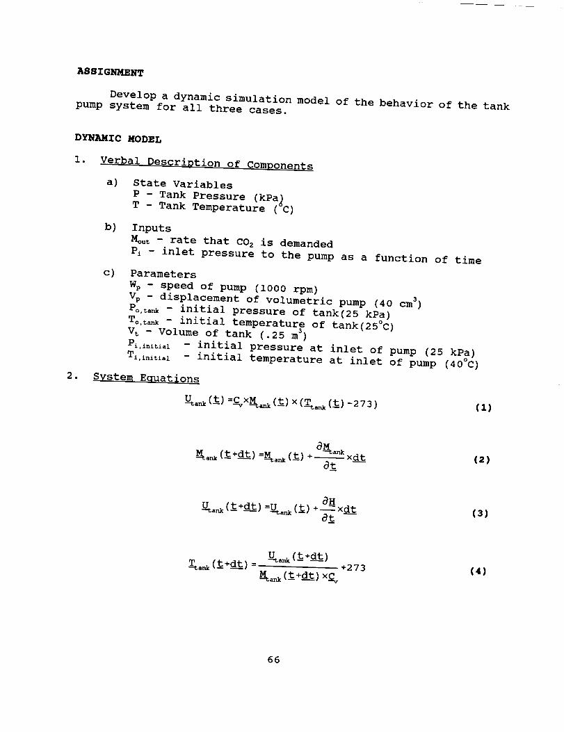
ASSIGNMENT

Develop a dynamic simulation model of the behavior of the tank

pump system for all three cases.

DYNAMIC MODEL

I. Verbal Description of Components

a) State Variables

P - Tank Pressure (kPa)T - Tank Temperature (vC)

b) Inputs

Mout - rate that CO 2 is demanded

P± - inlet pressure to the pump as a function of time

c) Parameters

Wp - speed of pump (I000 rpm)

Vp - displacement of volumetric pump (40 cm 3)

Po,ta_ - initial pressure of tank(25 kPa)

To,tan - initial temperature of tank(25°C)

Vt - Volume of tank (.25 m S)

Pi,lnitial - initial pressure at inlet of pump (25 kPa)

Ti.lniti.I - initial temperature at inlet of pump (40°C)

2. System Equations

U__a_k(_t_t):C_,,X_m_k(_.t)X (T._ (_t)-273 )

_a_ (t+dt) =M_ank (t) + -- xd__tat

(2)

aHU__,_ (t+dt) :U__ (t) +--_--xd__tt

at(3)

U__,_k(t +dt)

TT._.,_k(t+dt) - +273M___a_k(t+dt) ×Cv

(4)

66

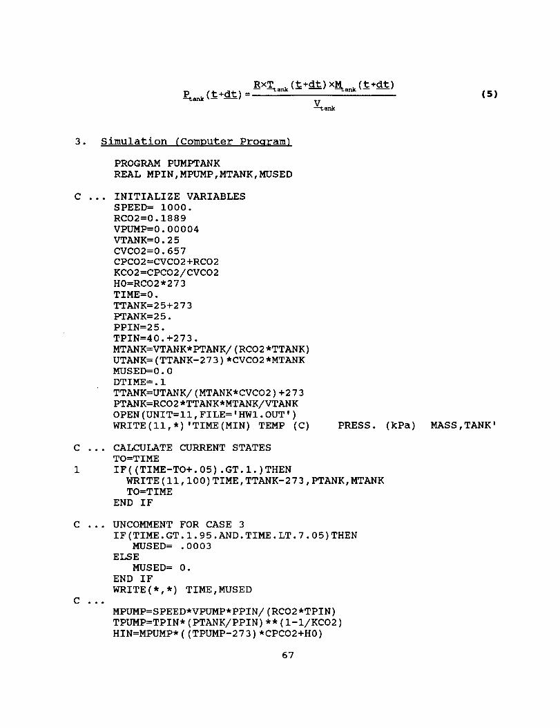
P--t_ (t+dt) =

RxTt_ (t+dt) ×_ (t+dt)

V-_ank

(s)

3. Simulation (Computer Program)

C

C

1

C

C

PROGRAM PUMPTANK

REAL MPIN,MPUMP,MTANK,MUSED

INITIALIZE VARIABLES

SPEED= i000.

RCO2=0.1889

VPUMP=0.00004

VTANK=0.25

CVCO2=0.657

CPCO2=CVCO2+RCO2

KCO2=CPCO2/CVC02

H0=RCO2*273

TIME=0.

TTANK=25+273

PTANK=25.

PPIN=25.

TPIN=40.+273.

MTANK=VTANK*PTANK/(RCO2*TTANK)

UTANK=(TTANK-273)*CVCO2*MTANKMUSED=0.0

DTIME=.I

TTANK=UTANK/(MTANK*CVC02)+273

PTANK=RCO2*TTANK*MTANK/VTANK

OPEN(UNIT=II,FILE='HWI.OUT')

WRITE(II,*) 'TIME(SIN) TEMP (C) PRESS.

CALCULATE CURRENT STATES

TO=TIME

IF( (TIME-TO+. 05) .GT. i. )THEN

WRITE(II,100)TIME,TTANK-273,PTANK,MTANKTO=TIME

END IF

UNCOMMENT FOR CASE 3

IF (TIME.GT. I. 95.AND.TIME. LT. 7.05)THENMUSED= .0003

ELSE

MUSED= 0.

END IF

WRITE (*, *) TIME, MUSED

MPUMP=S PEE D*VPUMP* PPIN/(RCO2 *TPIN)

TPUMP=TPIN* (PTANK/PPIN) * * (i- I/KCO2 )

HIN=MPUMP* ((TPUMP-273) *CPCO2+H0)

67

(kPa) MASS,TANK'

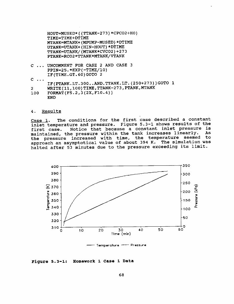
HOUT=MUSED*((TTANK-273)*CPCO2+H0)TIME=TIME+DTIME

MTANK=MTANK+(MPUMP-MUSED)*DTIME

UTANK=UTANK+(HIN-HOUT)*DTIME

TTANK=UTANK/(MTANK*CVCO2)+273

PTANK=RCO2*TTANK*MTANK/VTANK

C ... UNCOMMENT FOR CASE 2 AND CASE 3

PPIN=25.*EXP(-TIME/10)

IF(TIME.GT.60)GOTO 2

C ..o

2

i00

IF(PTANK. LT. 300..AND.TTANK. LT. (250+273)) GOTO 1

WRITE (11,100 )TIME, TTANK-273 ,PTANK, MTANK

FORMAT (F5.2,3 (2X, FI0.4) )

END

4. Results

Case i. The conditions for the first case described a constant

inlet temperature and pressure. Figure 5.3-1 shows results of thefirst case. Notice that because a constant inlet pressure is

maintained, the pressure within the tank increases linearly. As

the pressure increased with time, the temperature seemed to

approach an asymptotical value of about 394 K. The simulation washalted after 53 minutes due to the pressure exceeding its limit.

400

390

38O

v 570

,360U

_; 350

E 340

330

320

3100 1C1 2'0 3'0 4-'0 5'0

Time (rnln)

350

-300

-250

Q-v

-200 --_

@

150

Q

100

5O

060

-- Temperoture -- Pressure

Figure 5.3-i: Homework 1 Case 1 Data

68

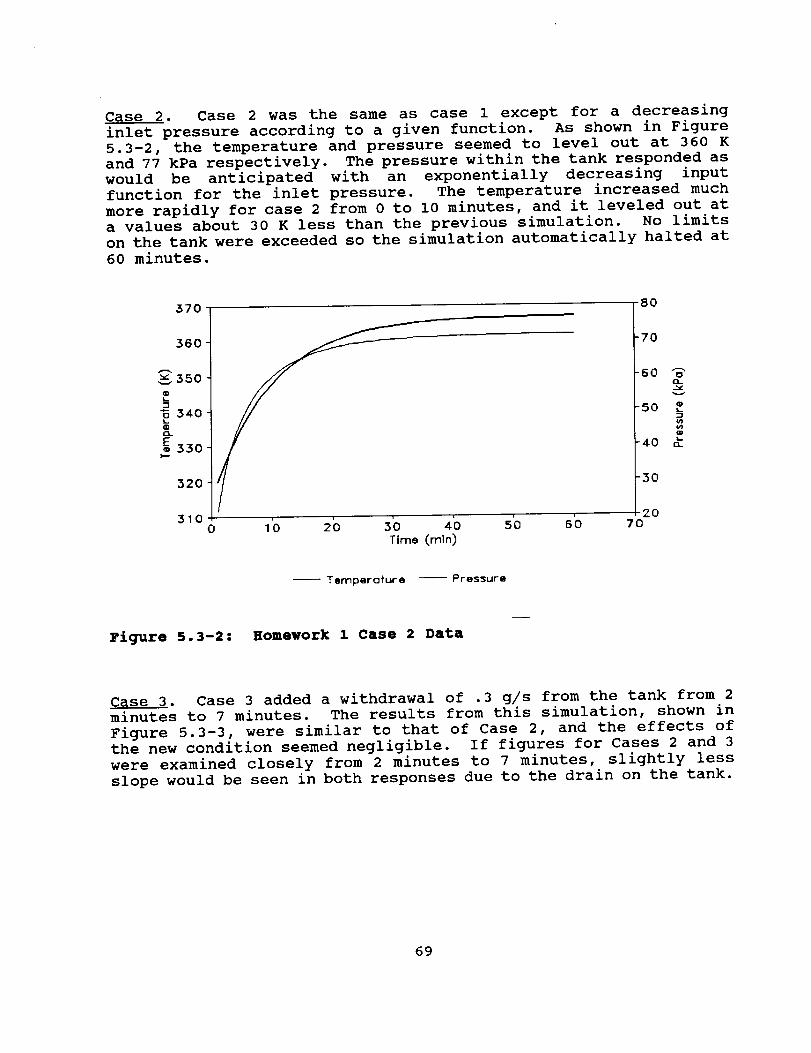
Case 2. Case 2 was the same as case 1 except for a decreasing

inlet pressure according to a given function. As shown in Figure

5.3-2, the temperature and pressure seemed to level out at 360 K

and 77 kPa respectively. The pressure within the tank responded as

would be anticipated with an exponentially decreasing input

function for the inlet pressure. The temperature increased much

more rapidly for case 2 from 0 to i0 minutes, and it leveled out at

a values about 30 K less than the previous simulation. No limits

on the tank were exceeded so the simulation automatically halted at

60 minutes.

370 8o

.560

350

340

330

320

310

I

-7O

-60 %"EL

-50 _"

o

-4.0 __

-3o

2o0 1'0 20 3'0 4'0 5'0 6'0 70

Time (nnln)

-- Tarnperofure -- Pressure

Figure 5.3-2: Homework i Case 2 Data

Case 3. Case 3 added a withdrawal of .3 g/s from the tank from 2

minutes to 7 minutes. The results from this simulation, shown in

Figure 5.3-3, were similar to that of Case 2, and the effects of

the new condition seemed negligible. If figures for Cases 2 and 3

were examined closely from 2 minutes to 7 minutes, slightly less

slope would be seen in both responses due to the drain on the tank.

69

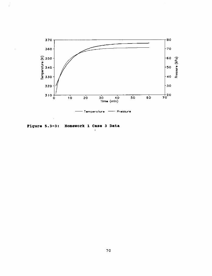
370

360

_350@

340Q

330

320

310

f

0

Time (rain)

5'0 sb

8O

-7O

-60QL-

-50

o

-4o _.

-30

2070

-- Temperafure --Pressure

Figure 5.3-3 : Homework 1 Case 3 Data

i

7O

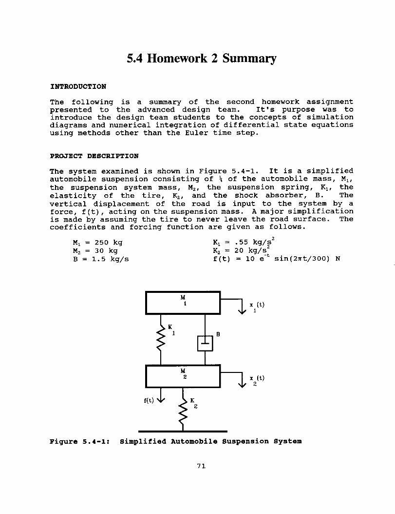
5.4 Homework 2 Summary

INTRODUCTION

The following is a summary of the second homework assignment

presented to the advanced design team. It's purpose was to

introduce the design team students to the concepts of simulation

diagrams and numerical integration of differential state equations

using methods other than the Euler time step.

PROJECT DESCRIPTION

The system examined is shown in Figure 5.4-1. It is a simplified

automobile suspension consisting of % of the automobile mass, MI,

the suspension system mass, M2, the suspension spring, KI, the

elasticity of the tire, K2, and the shock absorber, B. The

vertical displacement of the road is input to the system by a

force, f(t), acting on the suspension mass. A major simplification

is made by assuming the tire to never leave the road surface. The

coefficients and forcing function are given as follows.

M I = 250 kg

M 2 = 30 kg

B = i. 5 kg/s

K I = .55 kg/s 2

K 2 = 20 kg/s z

f(t) = i0 e -t sin(2_t/300) N

x CO1

x (t)2

Figure 5.4-1: Simplified Automobile Suspension System

71

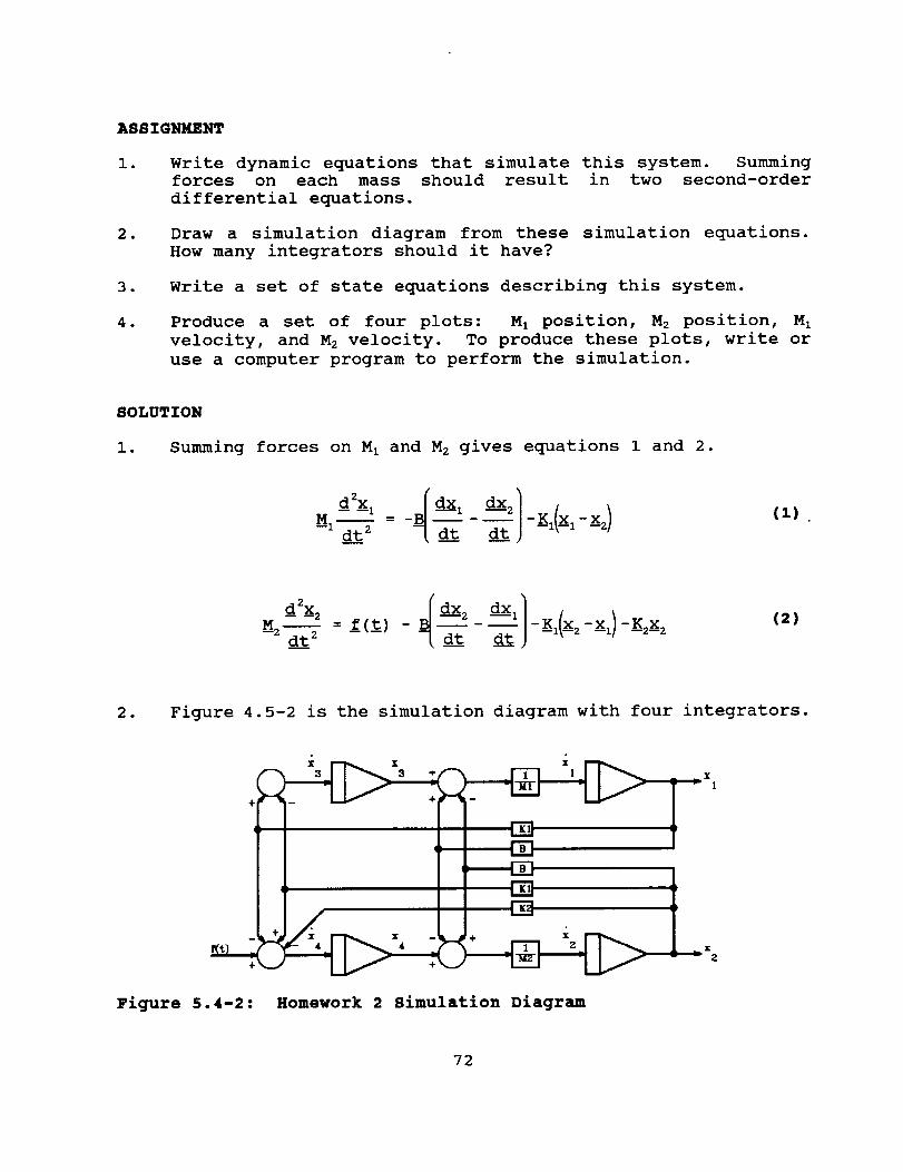
ASSIGNMENT

l. Write dynamic equations that simulate this system. Summingforces on each mass should result in two second-order

differential equations.

• Draw a simulation diagram from these simulation equations.

How many integrators should it have?

3. Write a set of state equations describing this system.

• Produce a set of four plots: M I position, M2 position, M I

velocity, and M 2 velocity. To produce these plots, write or

use a computer program to perform the simulation.

SOLUTION

i. Summing forces on M I and M 2 gives equations 1 and 2.

0x40x ldt 2 _ dt )

(1)

M 2

d2x2

dt 2dx2 dxl 1-- f(t) -- d_ - _ -KI(X2-X1)-K2x2

(2)

2. Figure 4.5-2 is the simulation diagram with four integrators•

• °

• • X

÷

Figure 5.4-2: Homework 2 Simulation Diagram

72

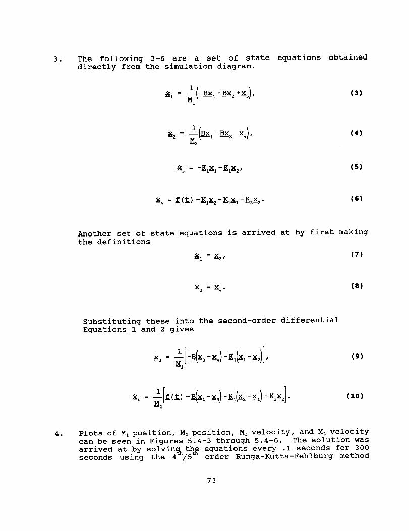
• The following 3-6 are a set of state equations obtained

directly from the simulation diagram•

__i = -_I (-Bxl + Bx2 +x3),

MI(3)

__2 = l(Bx_-Bx2 x4),M2

(4)

-_3= -KIxl +KIx2' (s)

_x4 = f (t) -KIx2+KIX I-K2x 2. (6)

Another set of state equations is arrived at by first making

the definitions

-xl= x3' (7)

_2 = x4" (8)

Substituting these into the second-order differential

Equations 1 and 2 gives

1 x (9)

_4 = u

M2(lO)

• Plots of M I position, M2 position, MI velocity, and M 2 velocity

can be seen in Figures 5.4-3 through 5•4-6• The solution was

arrived at by solvina the equations every .i seconds for 300

seconds using the 4_h/5 th order Runga-Kutta-Fehlburg method

73

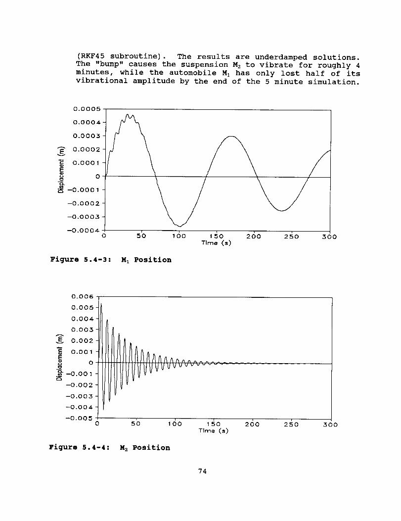
(RKF45 subroutine). The results are underdamped solutions.The "bump" causes the suspension Mz to vibrate for roughly 4minutes, while the automobile MI has only lost half of itsvibrational amplitude by the end of the 5 minute simulation.

0.0005

0.0004

0.0003

E 0.0002

0.0001

E_ 0

5 --0.0001

--0.0002

--0.0003

--O.OOO40 5'0 160 150 260 250 300

Time (s)

Figure 5.4-3: MI Position

0.006

0.005

0.00_

0.003

E 0.002

0.001E

o

_- -0.001r-,,,

--0.002

--0.003

--0.004

--0.005o sB 16o 1so 260 2so

Time (S)

Figure 5.4-4: M z Position

300

74

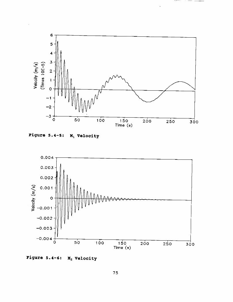
6

5

4

3

_ _ o

--1 ,

-2

-30 sb 16o I,_O 260 2_o 300

Time (s)

Figure 5.4-5: Mz Velocity

0,004

0.003

0.002

0.001

E0

o-0.001>

-0.002

-0.003

--0.004o 5b 16o i_o

Time (s)260 2so 3OO

Figure 5.4-6: Ms Velocity

75

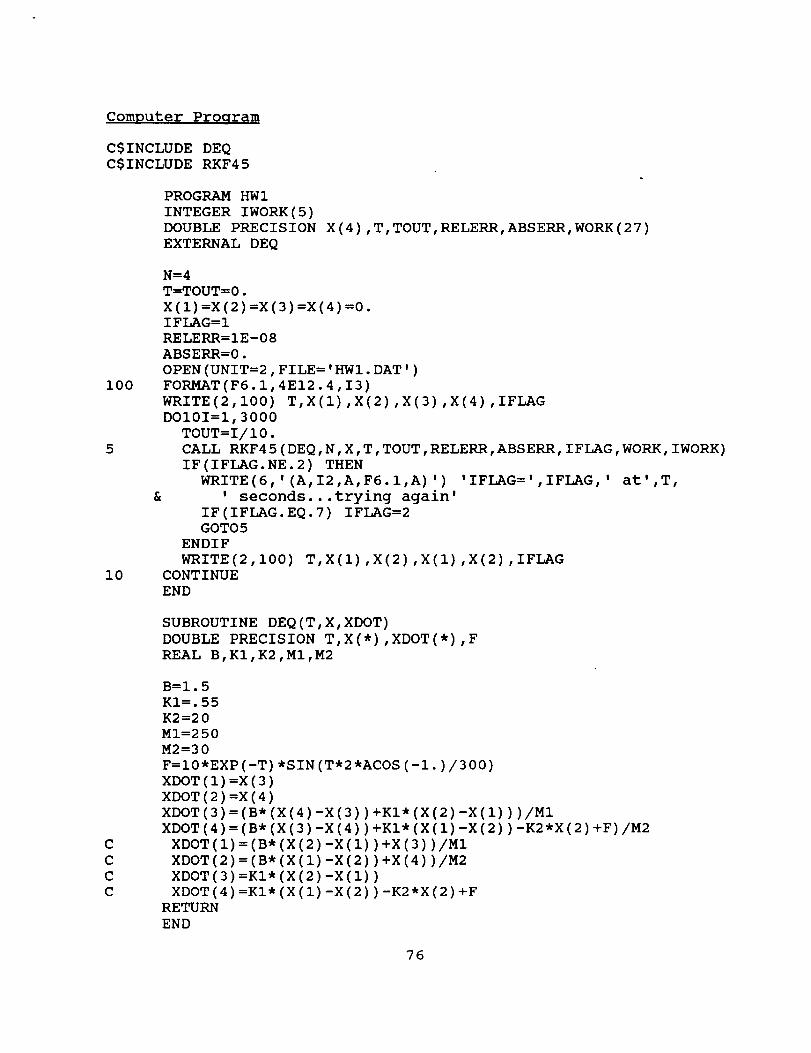
Computer Proqram

C$INCLUDE DEQ

C$INCLUDE RKF45

PROGRAM HWI

INTEGER IWORK(5)

DOUBLE PRECISION

EXTERNAL DEQ

X (4 ), T, TOUT, RELERR, ABSERR, WORK (27 )

I00

5

i0

&

N=4

T=TOUT=0.

X(1) =X(2) =X(3) =X(4) =0.IFLAG=I

RELERR=IE-08

ABSERR=0.

OPEN (UNIT=2, FILE= 'HWI. DAT ')

FORMAT (F6. i, 4E12 .4, I3)

WRITE (2, I00) T, X(1) ,X(2) ,X(3) ,X(4) ,IFLAG

DOIOI=I, 3000

TOUT=I/10.

CALL RKF45 (DEQ, N, X, T, TOUT, RELERR, ABSERR, IFLAG, WORK, IWORK)

IF (IFLAG.NE. 2) THEN

WRITE(6,'(A, I2,A,F6.I,A)') 'IFLAG=',IFLAG,' at',T,

' seconds...trying again'

IF (IFLAG. EQ. 7) I FLAG=2

GOTO5

ENDIF

WRITE(2,100) T,X(1) ,X(2) ,X(1),X(2) ,IFLAG

CONTINUE

END

SUBROUTINE DEQ(T,X,XDOT)

DOUBLE PRECISION T,X(*),XDOT(*),F

REAL B,KI,K2,MI,M2

C

C

C

C

B=I.5

KI=. 55

K2 =20

MI=250

M2=30

F=I0*EXP (-T) *SIN (T*2 *ACOS (-i. )/300 )

XDOT (1 )=X (3 )

XDOT (2 )=X (4 )

XDOT (3) =(B* (X(4) -X(3) )+El* (X(2) -X(1) ) )/Sl

XDOT (4)= (B* (X (3)-X(4) )+El* (X (i)-X(2) )-K2*X (2) +F)/S2

XDOT (i)= (B* (X (2)-X(1) )+X (3))/Sl

XDOT (2)= (B* (X (i)-X(2) )+X (4))/S2

XDOT (3)=El* (X(2) -X(1) )

XDOT (4) =KI* (X (i) -X (2)) -K2*X (2) +F

RETURN

END

76

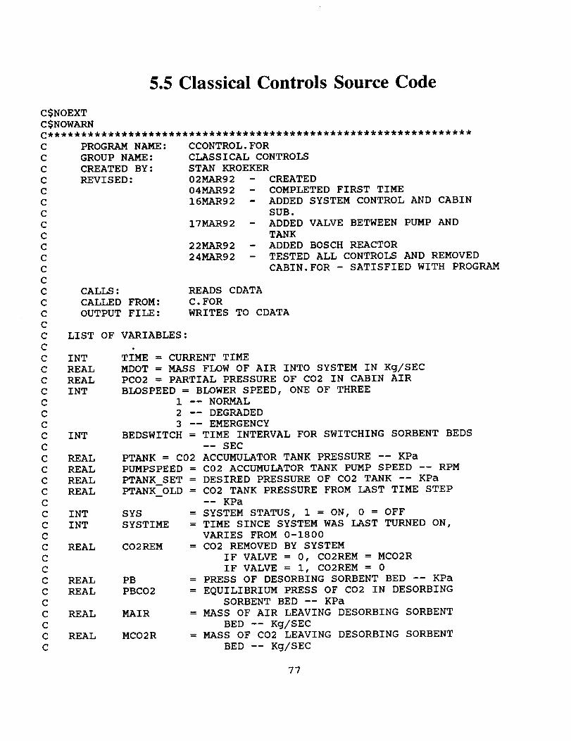
5.5 Classical Controls Source Code

C

C

C

C

C

C

C

C

C

C

C

C

C

C

C

C

C

C

C

C

C

C

C

C

C

C

C

C

C

C

C

C

C

C

C

C

C

C

C

C

C

C

C

C

C

C

PROGRAM NAME:

GROUP NAME:

CREATED BY:

REVISED:

CCONTROL.FOR

CLASSICAL CONTROLS

STAN KROEKER

02MAR92

04MAR92

16MAR92

17MAR92

22MAR92

24MILR92

- CREATED

- COMPLETED FIRST TIME

- ADDED SYSTEM CONTROL AND CABIN

SUB.

- ADDED VALVE BETWEEN PUMP AND

TANK

- ADDED BOSCH REACTOR

- TESTED ALL CONTROLS AND REMOVED

CABIN.FOR - SATISFIED WITH PROGRAM

CALLS:

CALLED FROM:

OUTPUT FILE:

READS CDATA

C.FOR

WRITES TO CDATA

LIST OF VARIABLES:

INT TIME = CURRENT TIME

REAL MDOT = MASS FLOW OF AIR INTO SYSTEM IN Kg/SEC

REAL PCO2 = PARTIAL PRESSURE OF CO2 IN CABIN AIR

INT BLOSPEED = BLOWER SPEED, ONE OF THREE

1 -- NORMAL

2 -- DEGRADED

3 -- EMERGENCY

INT BEDSWITCH = TIME INTERVAL FOR SWITCHING SORBENT BEDS

-- SEC

REAL PTANK = C02 ACCUMULATOR TANK PRESSURE -- KPa

REAL PUMPSPEED = C02 ACCUMULATOR TANK PUMP SPEED -- RPM

REAL PTANK SET = DESIRED PRESSURE OF C02 TANK -- KPa

REAL PTANK OLD = CO2 TANK PRESSURE FROM LAST TIME STEP

-- KPa

INT SYS = SYSTEM STATUS, 1 = ON, 0 = OFF

INT SYSTIME = TIME SINCE SYSTEM WAS LAST TURNED ON,

VARIES FROM 0-1800

REAL CO2REM = CO2 REMOVED BY SYSTEM

IF VALVE = 0, C02REM = MCO2R

IF VALVE = I, CO2REM = 0

REAL PB = PRESS OF DESORBING SORBENT BED -- KPa

REAL PBCO2 = EQUILIBRIUM PRESS OF CO2 IN DESORBING

SORBENT BED -- KPa

REAL MAIR = MASS OF AIR LEAVING DESORBING SORBENT

BED -- Kg/SEC

REAL MCO2R = MASS OF C02 LEAVING DESORBING SORBENT

BED -- Kg/SEC

77

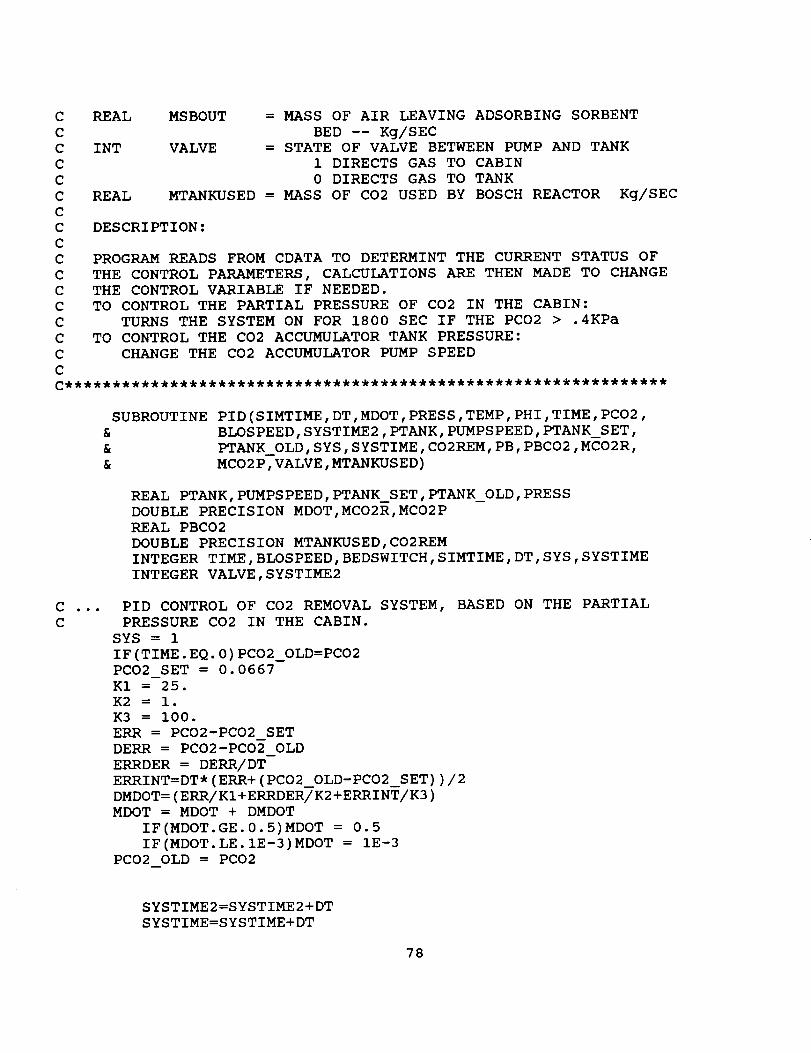
CCCCCCCCCCCCCCCCC

REAL

INT

REAL

MSBOUT = MASS OF AIR LEAVING ADSORBING SORBENT

BED -- Kg/SEC

VALVE = STATE OF VALVE BETWEEN PUMP AND TANK

1 DIRECTS GAS TO CABIN

0 DIRECTS GAS TO TANK

MTANKUSED = MASS OF C02 USED BY BOSCH REACTOR Kg/SEC

DESCRIPTION:

PROGRAM READS FROM CDATA TO DETERMINT THE CURRENT STATUS OF

THE CONTROL PARAMETERS, CALCULATIONS ARE THEN MADE TO CHANGE

THE CONTROL VARIABLE IF NEEDED.

TO CONTROL THE PARTIAL PRESSURE OF CO2 IN THE CABIN:

TURNS THE SYSTEM ON FOR 1800 SEC IF THE PC02 > .4KPa

TO CONTROL THE C02 ACCUMULATOR TANK PRESSURE:

CHANGE THE CO2 ACCUMULATOR PUMP SPEED

SUBROUTINE PID(SIMTIME,DT,MDOT,PRESS,TEMP,PHI,TIME,PCO2,

& BLOSPEED,SYSTIME2,PTANK, PUMPSPEED,PTANK_SET,

& PTANK OLD,SYS,SYSTIME,CO2REM,PB,PBCO2,MCO2R,

& MCO2P,VALVE,MTANKUSED)

REAL PTANK,PUMPSPEED,PTANK_SET,PTANK_OLD,PRESS

DOUBLE PRECISION MDOT,MCO2R,MCO2P

REAL PBCO2

DOUBLE PRECISION MTANKUSED,CO2REM

INTEGER TIME,BLOSPEED,BEDSWITCH,SIMTIME,DT,SYS,SYSTIME

INTEGER VALVE,SYSTIME2

C ,..

C

PID CONTROL OF CO2 REMOVAL SYSTEM, BASED ON THE PARTIAL

PRESSURE CO2 IN THE CABIN.

SYS = 1

IF (TIME. EQ. 0) PCO2_OLD=PCO2PCO2 SET = 0.0667

K1 = 25.

K2 = i.

K3 = I00.

ERR = PCO2-PCO2 SET

DERR = PCO2-PCO2 OLD

ERRDER = DERR/DT

ERRINT=DT*(ERR+(PCO2_OLD-PCO2_SET))/2

DMDOT= (ERR/KI+ERRDER/K2 +ERRINT/K3 )

MDOT = MDOT + DMDOT

IF(MDOT.GE.0.5)MDOT = 0.5

IF(MDOT.LE.IE-3)MDOT = IE-3

PCO2 OLD = PCO2

SYSTIME2=SYSTIME2+DT

SYSTIME=SYSTIME+DT

78

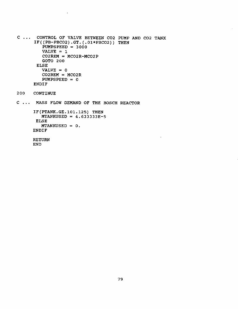
C , • • CONTROL OF VALVE BETWEEN CO2 PUMP AND CO2 TANK

IF((PB-PBCO2) .GT. (.01*PBCO2)) THENPUMPSPEED = 3000

VALVE = 1

C02REM = MCO2R-MCO2P

GOTO 200

ELSE

VALVE = 0

C02REM = MCO2R

PUMPSPEED = 0

ENDIF

CONTINUE

MASS FLOW DEMAND OF THE BOSCH REACTOR

IF(PTANK.GE.101.125) THENMTANKUSED = 4.633333E-5

ELSE

MTANKUSED = 0.

ENDIF

RETURN

END

79

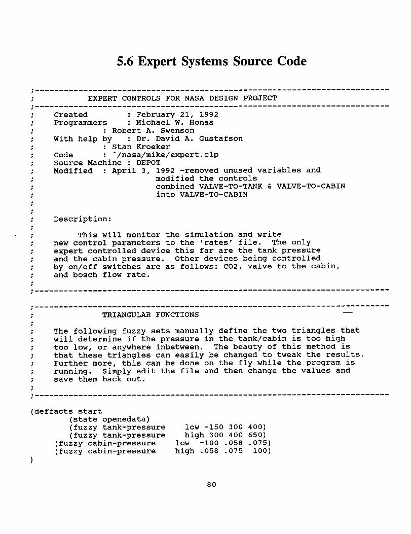
5.6 Expert Systems Source Code

EXPERT CONTROLS FOR NASA DESIGN PROJECT

Created : February 21, 1992

Programmers : Michael W. Honas: Robert A. Swenson

With help by : Dr. David A. Gustafson: Stan Kroeker

Code : "/nasa/mike/expert.clp

Source Machine : DEPOT

Modified : April 3, 1992 -removed unused variables andmodified the controls

combined VALVE-TO-TANK & VALVE-TO-CABIN

into VALVE-TO-CABIN

Description:

This will monitor the simulation and write

new control parameters to the 'rates' file. The only

expert controlled device this far are the tank pressure

and the cabin pressure. Other devices being controlled

by on/off switches are as follows: CO2, valve to the cabin,

and bosch flow rate.

TRIANGULAR FUNCTIONS

The following fuzzy sets manually define the two triangles that

will determine if the pressure in the tank/cabin is too high

too low, or anywhere inbetween. The beauty of this method is

that these triangles can easily be changed to tweak the results.

Further more, this can be done on the fly while the program is

running. Simply edit the file and then change the values and

save them back out.

(deffacts start

(state openedata)

(fuzzy tank-pressure

(fuzzy tank-pressure

(fuzzy cabin-pressure

(fuzzy cabin-pressure

low -150 300 400)

high 300 400 650)

low -i00 .058 .075)

high .058 .075 I00)

80

_----m----m

OPEN-edata

Read in the values from the Fortran and C simulation modules.

"edata" is a temporary file that is used to pass variables

between the simulation and the clips control. This is done

simply because we cannot link CLIPS in with any other compiler.

This is one of the few draw backs is that it is almost a closed

system.

(defrule open-edata

?s <- (state openedata)

=>

; (printout t "Entering open expert data" crlf)

(retract ?s)

(open "edata" data "r+")

(assert (time-step

(assert (mass-in

(assert (partial-co2

(assert (tank-pressure

(assert (pump-speed =(read data)))

=(read data)))

=(read data)))

=(read data)))

=(read data)))

(assert (sys

(assert (sys-time

(assert (sys-2time

(assert (co2-rem

(assert (pb

(assert (pbco2

(assert (mco2p

(assert (mco2r

(assert (valve

(assert (mtankused

=(read data)))

=(read data)))

=(read data)))

=(read data)))

=(read data)))

=(read data)))

=(read data)))

=(read data)))

=(read data)))

=(read data)))

(close data)

(assert (state control-pp))

CONTROL-PC02

This rule controls the partial pressure of the carbon dioxide

and also takes care of the system time.

(defrule control-pco2

?s <- (state control-pp)

?f <- (sys ?sy)?h <- (sys-time ?st)

?i <- (sys-2time ?s2t)

?j <- (mass-in ?mi)

81

(partial-co2 ?pc)(time-step ?ts)

_->(printout t "Entering CONTROL-PC02" crlf)

(retract ?s)

(if (= ?sy i) then

(retract ?i)

(assert (sys-2time =(+ ?s2t ?ts)))

)

(if (and (and (= ?sy i) (>= ?st 1800))(<= ?pc .4)) then

(retract ?f)

(retract ?h)

(retract ?j)

(assert (sys 0))

(assert (sys-time 0))

(assert (mass-in 0))else

(if (and (= ?sy 0) (>= ?pc .4)) then

(retract ?f)

(retract ?j)

(assert (sys I))

(assert (sys-time 0))

(assert (mass-in .5))else

(if (and (and (= ?sy i) (>= ?st 1800))(> ?pc .4)) then

(retract ?h)

(assert (sys-time 0))

(assert (state valve))else

(if (and (= ?sy i) (< ?st 1800)) then

(retract ?h)

(assert (sys-time =(+ ?ts ?st)))

))))

(assert (state valve))

VALVE-TO-CABIN

This system will turn the valve on and off and assert a

pump speed of 3000 if necessary.

(defrule valve-to-cabin

?s <- (state valve)

(pb ?pb)

82

(pbco2 ?p2)?f <- (pump-speed ?ps)?g <- (valve ?va)?h <- (co2-rem ?_o)(mco2p ?mcp)(mco2r ?mcr)

=>(printout t "Entering VALVE-TO-CABIN" crlf)(retract ?s)(retract ?g)(retract ?h)

(if (> (- ?pb ?p2)then

else

(* ?p2 0.01)) ; if pb >> p2

(retract ?f)

(assert (pump-speed 3000))

(assert (valve I))

(assert (co2-rem =(- ?mcr ?mcp)))

(assert (state bosch))

(assert (valve 0))

(assert (co2-rem ?mcr))

(assert (state calc))

; CALC-MEMBERSHIP-FOR-PUMP

; Calculate the percent belief that the tank pressure or cabin

; pressure is low, right or high.

;_Imm ....

(defrule calc-membership

(state calc)

(fuzzy ?var ?qual ?low ?mid ?high)

(?var ?val)=>

(printout t "Entering CALC-MEMBERSHIP-FOR-PUMP" crlf)

(if (and (> ?val ?low) (<= ?val ?mid)) then

(assert (member ?var ?qual =(/ (- ?val ?low) (- ?mid ?low)))))

(if (and (> ?val ?mid) (< ?val ?high)) then

(assert (member ?var ?qual =(/ (- ?high ?val) (- ?high ?mid)))))

RULES

This rule decides whether an action should take place.

83

That action is based on the belief of better than 50%

(defrule rules(state calc)?f <- (member ?variable ?quality ?val&:(> ?val .5))

=>; (printout t "Entering RULES" crlf)

(retract ?f)(assert (action ?variable ?quality ?val))

I

; NO-CHANGES

; Conversly, this rule decides that no action should take place

; if the belief is 50% or less.

(defrule no-changes

(state calc)

?f <- (member ?variable ?quality ?val&:(<= ?val .5))=>

; (printout t "Entering NO-CHANGES" crlf)

(retract ?f)

ACTION-SLOW-MOTOR

This rule will slow the motor by some variable amount

based on the percent belief.

(defrule action-slow-motor

(state calc)

?fm <- (action tank-pressure high ?val)

?ps <- (pump-speed ?wps)=>

; (printout t "Entering ACTION-SLOW-MOTOR" crlf)

(retract ?fm)

(retract ?ps)

(if (< ?val (/ ?wps 3000)) then (assert (pump-speed =

(- ?wps (* i00 ?val))))

else (assert (pump-speed 0)))

84

ACTION-FAST-MOTOR

This rule will speed up the motor by some variable amountbased on the percent belief.

(defrule action-fast-motor(state calc)?fm <- (action tank-pressure low ?val)?ps <- (pump-speed ?wps)

=>(printout t "Entering ACTION-FAST-MOTOR" crlf)(retract ?fm)(retract ?ps)(if (> ?val (/ ?wps 3000)) then (assert (pump-speed =

(+ ?wps (* i00 ?val))))else (assert (pump-speed 3000)))

ACTION-SLOW-MDOT

This rule will slow down the mass flow rate by some variable amountbased on the percent belief.

(defrule action-slow-mdot(state calc)?fm <- (action cabin-pressure high ?val)?ps <- (mass-in ?mi)

=>

; (printout t "Entering ACTION-SLOW-MDOT" crlf)

(retract ?fm)

(retract ?ps)

(if (< ?val (/ ?mi .5)) then (assert (mass-in =

(- ?mi (* .05 ?val))))

else (assert (mass-in 0)))

-w--w--------------------.¢

ACTION-FAST-MDOT

This rule will speed up the mass flow rate by some variable amount

based on the percent belief.

85

(defrule action-fast-mdot(state calc)?fm <- (action cabin-pressure low ?val)?ps <- (mass-in ?mi)

=>(printout t "Entering ACTION-FAST-MDOT" crlf)(retract ?fm)(retract ?ps)(if (> ?val (/ ?mi .5)) then (assert (mass-in =

(+ ?mi (* .05 ?val))))else (assert (mass-in .5)))

CALC-DONE

This will end the calculations and adjustments made forthe fuzzy logic sets. Notice that there is a salience of -i0.This is so that the calculations can complete recursively untilthey are all done.

(defrule calc-done(declare (salience -I0))?s <- (state calc)

=>(printout t "Entering CALC-DONE" crlf)

(retract ?s)

(assert (state bosch))

I

BOSCH-MASS-FLOW

This rule will change the mass in the tank used depending

on whether the tank pressure is above or below 101.125.

(defrule bosch-mass-flow

?s <- (state bosch)

(tank-pressure ?tp)

?f <- (mtankused ?mt)

_->

(printout t "Entering BOSCH-MASS-FLOW" crlf)

(retract ?s)

(retract ?f)

(if (>= ?tp 101.125) then

(assert (mtankused .000046333))

86

)(if (< ?tp 101.125) then

(assert (mtankused 0) )

)(assert (state bosch-sys))

_m_mmmm_m_u°

BOSCH-SYSTEM

(defrule bosch-system

_->

?s <- (state bosch-sys)

(tank-pressure ?tp)

?g <- (sys ?sy)

?h <- (sys-time ?st)

?i <- (mass-in ?mi)

(printout t "Entering BOSCH-SYSTEM" crlf)

(retract ?s)

(if (and (< ?tp 137.000)

(retract ?g)

(retract ?h)

(retract ?i)

(assert (sys i))

(assert (sys-time 0))

(assert (mass-in .5))

)(assert (state writeedata))

(= ?sy 0)) then

WRITE-edata

Write in the values for the Fortran and simulation modules.

(defrule write-edata

?s <- (state writeedata)

?ts <- (time-step ?wts)

?mi <- (mass-in ?wmi)

?pc <- (partial-co2 ?wpc)

?tp <- (tank-pressure ?wtp)

?ps <- (pump-speed ?wps)

?sy <- (sys ?wsy)?st <- (sys-time ?wst)

87

=>

?st2 <- (sys-2time ?wst2)?co <- (co2-rem ?wco)?pb <- (pb ?wpb)?p2 <- (pbco2 ?wp2)

?ma <- (mco2p ?wma)

?mc <- (mco2r ?wmc)

?va <- (valve ?wva)

?mt <- (mtankused ?wmt)

(printout t "Entering write expert data" crlf)

(retract ?s)

(retract ?ts)

(retract ?mi)

(retract ?pc)

(retract ?tp)

(retract ?ps)

(retract ?sy)

(retract ?st)

(retract ?st2)

(retract ?co)

(retract ?pb)

(retract ?p2)

(retract ?ma)

(retract ?mc)

(retract ?va)

(retract ?mt)

(system "rm edata")

(open "edata" data "w")

(printout data ?wts crlf)

(printout data ?wmi crlf)

(printout data ?wpc crlf)

(printout data ?wtp crlf)

(printout data ?wps crlf)

(printout data ?wsy crlf)

(printout data ?wst crlf)

(printout data ?wst2 crlf)

(printout data ?wco crlf)

(printout data ?wpb crlf)

(printout data ?wp2 crlf)

(printout data ?wma crlf)

(printout data ?wmc crlf)

(printout data ?wva crlf)

(printout data ?wmt crlf)

(close data)

88

C$NOEXTC$NOWARNC$TIME=36000C$INCLUDE SIMC$INCLUDE PID

C$INCLUDE EXP

* CREATED BY:

* CREATED:

5.7 Simulation Source Code

STAN KROEKER

APRIL I, 1992

THIS PROGRAM IS TO TEST THE SIMULATION AND THE CONTROLS

PROGRAM COOL

DOUBLE PRECISION MDOT,MAIR,MCO2R,MCO2P,MTANKUSED,CO2REM,MCO2

INTEGER SIMTIME,DT,TIME,BLOSPEED,BEDSWITCH,SYSTIME,SYS,VALVE,IINTEGER SYSTIME2

C ... REAL DESSICANT BED VALUES

REAL MDBADS (2,2 ) ,MDBTANK (2 )

C ... REAL SORBENT BED AND SORBENT PUMP VALUES

REAL MSBTANK (3 ) ,MSBADS (2,3) ,TBED (2,3)

C ... REAL CO2 TANK VALUES

DOUBLE PRECISION MTANK,MTIN,MTOUT

* INITIALIZE VARIABLES

SIMTIME = 0

SYSTIME2 = 0

DT = 6

MDOT = 0

PRESS = 101.125

TEMP = 300

PHI = .78

TIME = 0

PCO2 = .0667

BLOSPEED = 0

BEDSWITCH = 0

PTANK = 300

PUMPSPEED = 0

PTANK SET = 350

PTANK OLD = 101.125

SYS = 0

SYSTIME = 0

CO2REM = 0

PB = 101.125

89

PBCO2 = .0667M.AIR = 0

MCO2R = 0

MCO2P = 0

VALVE = 0

MTANKUSED = 0

I=0

J=0

CPAIR=I. 006

MDBTANK (I) =I00.

MDBTANK (2 )= 100.

MDBADS (1,1) =0. 001

MDBADS (I, 2) =0. 001

MDBADS (2,1) =0. 001

MDBADS (2,2) =0. 001

C . . . BLOWER/PRECOOLER SUBROUTINE VARIABLE INITIALIZATION

i0 CPH20=4.184

EPSILON=.8

PAIR=I.1614

TWATER=288

VELAIR=3.

C ... SORBENT BED AND SORBENT PUMP SUBROUTINE VARIABLE

C ... INITIALIZATION

CPAIR=I.006

CVAIR=.719

CVBED=I.

CVCO2=.7

HCO2=572.

HEAT=0.

MCO2=0.

MAIR=.I

MSBADS(I,I)=0.

MSBADS(I,2)=0.

MSBADS(I,3)=0.

MSBADS (2, I) =0.

MSBADS (2,2) =0.

MSBADS (2,3) =0.

MSBTANK(1) = 30.

MSBTANK(2) = 30.

MSBTANK(3) = 30.PBED=I01.325

PSPIN=I01.325

RAIR=.287

RCO2=.1889

SPEED=3000

TBED(I,I)=300.

TBED(I,2)=300.

TBED(I,3)=300.

9O

TBED(2 , 1)=300.TBED(2,2) =300.

TBED(2,3) =300.

VBED=. 1

VPUMP = 0.0006

C ... CO2 TANK SUBROUTINE VARIABLE INITIALIZATION

MTANK=2.

TTANK= 300.

VTANK= 1.

MTOUT=0.

WRITE (*, *) 'Working... '

DO i00 TIME = 0,7500000,DT

IF(MOD(TIME,3600) .EQ.0) THEN

WRITE(*,*)'The time now is

J=J+l

',J,' hours....SYS = ',SYS

IF(J.EQ. 25) STOP

C

C

C

ENDIF

DETERMINE CONTROLLER TO UTILIZE

CALL PID(SIMTIME,DT,MDOT,PRESS,TEMP,PHI,TIME,PCO2,

& BLOSPEED,SYSTIME2,PTANK,PUMPSPEED,PTANK_SET,

& PTANK_OLD,SYS,SYSTIME,CO2REM,PB,PBCO2,MCO2R,

& MCO2P,VALVE,MTANKUSED)

CALL EXP(SIMTIME,DT,MDOT,PRESS,TEMP,PHI,TIME,PCO2,

BLOSPEED,SYSTIME2,PTANK, PUMPSPEED,PTANK_SET,

PTANK_OLD,SYS,SYSTIME,CO2REM,PB,PBCO2,MCO2R,

MCO2P,VALVE,MTANKUSED)

C

C

C

CALL MAIN SIMULATION

CALL

&

&

&

&

&

I=I+i

SIM(SIMTIME,DT,MDOT,PRESS,TEMP,PHI,TIME,

PCO2,BLOSPEED,MCO2,MAIR,PTANK, PUMPSPEED,

PTANK_SET,PTANK_OLD,SYS,SYSTIME2,CO2REM,

PB,PBCO2,MCO2R,MCO2P,VALVE,MTANKUSED,CPAIR,

MDBTANK,MDBADS,CPH20,EPSILON,PAIR,TWATER,VELAIR,

CVAIR,CVBED,CVCO2,HCO2,HEAT,MSBADS,MSBTANK,

RAIR,RCO2,TBED,VBED,VPUMP,MTANK,TTANK,VTANK,ADSORB,

DESORB,CO2ADSORB,CO2DESORB)

i00 CONTINUE

END

91

C oeeeeeeloeooooeee.o.eeeee,o,e,ee.e,,o,oe.,,eo.eoQ,e,,eeoeeeeo.o

C ... PROGRAM NAME: SIM.FOR

C ... GROUP NAME: CLASSICAL CONTROL

C ... CREATED BY: PAUL M. SNIDER, STAN KROEKER

C ................ MARCH 3, 1992

C ... REVISED: 03/10/92 (PS)C ... SUBROUTINE CALLS: DESSBED.FOR

C ...................... BLOWCOOL.FOR

C ...................... SORBED.FOR

C ...................... SORPUMP.FOR

C ...................... CO2TANK.FOR

C ...................... CWRITE.FOR -- (IN EXPERT SIM ONLY)

C ... CALLED FROM: CO2REM.FOR

C ... INPUT FILE: CREAD.FOR

C ... OUTPUT FILE: CWRITE.FOR

C ........................ LIST OF VARIABLES

C ee,eeeeeeeeeeoeee_aeeeeeeeeoeeoeeeeoooeooeeoooooooee_oeeeooeo,e

C ... SEE SUBROUTINES FOR LOCAL VARIABLE LIST

C _.t_._IQO_QQe_mleOSQS..SIOeOt...OOOOOQtQQ.tOOeQQQI.t_..IIQQIO..

C$NOEXT

C$NOWARN

C$INCLUDE DESSBED

C$INCLUDE BLOWCOOL

C$INCLUDE CWRITE

C$INCLUDE SORBED

C$INCLUDE S ORPUMP

C$ INCLUDE CO2TANK

C$INCLUDE CABIN

C$TIME=3600

SUBROUTINE SIM

&

&

&

&

&

&

&

(SIMTIME,DT,MDBIN, PDBIN,TDBIN,PHIIN,SYSTIME,

PCO2,BLOSPEED,MCO2,MAIR,PTANK,SPEED,

PTANK_SET,PTANK_OLD,SYS,TIME,CO2REM,

PBED,PVCO2,MCO2R,MCO2P,VALVE,MTOUT,CPAIR,

MDBTANK,MDBADS,CPH20,EPSILON,PAIR,TWATER,VELAIR,

CVAIR,CVBED,CVCO2,HCO2,HEAT,MSBADS,MSBTANK,

RAIR,RCO2,TBED,VBED,VPUMP,MTANK,TTANK,VTANK,ADSORB,

DESORB,CO2ADSORB,CO2DESORB)

C ... REAL DESSICANT BED VALUES

REAL MDBADS (2,2 ) ,MDBTANK (2 )

DOUBLE PRECISION MH20,MH2OR,MDBIN,MDBOUTI,MDBOUT2,MDBOUT3

C ... REAL BLOWER/PRECOOLER VALUES

DOUBLE PRECISION MBCIN,MBCOUT

C ... REAL SORBENT BED AND SORBENT PUMP VALUES

REAL MSBTANK(3),MSBADS(2,3) ,TBED(2,3)

DOUBLE PRECISION MAIR,MCO2,MCO2R,MCO2P,MSBOUT,MSPOUT,CO2REM

92

C ... REAL C02 TANK VALUES

DOUBLE PRECISION MTANK,MTIN,MTOUT

C ... DECLARE ALL INTEGERS FOR THE SIMULATION

INTEGER DT,T,TIME,BLOSPEED,BEDSWITCH,SIMTIME,SYS,SYSTIME,VALVE

C ... RUN CO2 REMOVAL ASSEMBLY SIMULATION AT A TIME STEP DT FOR A

C ... TIME DURATION T

CALL CABIN(TDBIN,PDBIN,PHIIN,DT,SYSTIME,CO2REM,PCO2)

IF(SYS.EQ.I) THEN

CALL DESSBED(MDBIN,PDBIN,PHIIN,TDBIN,MDBOUTI,PDBOUTI,PHI

& OUTI,TDBOUTI,CPAIR, DT,MDBADS,MH20,MH2OR,MDB

& TANK, I,TIME,ADSORB)

CALL BLOWCOOL(MDBOUTI,PDBOUTI,TDBOUTI,MBCOUT,PBCOUT,TBCO

& UT,CPH20,EPSILON,PAIR,TWATER,VELAIR)

CALL SORBED(MBCOUT,PBCOUT,TBCOUT,MSBOUT,PSBOUT,TSBOUT,CP

& AIR,_VBED,DT,HCO2,MSBADS,MSBTANK,PCO2

& ,PVCO2OUT,TBED,TIME,CO2ADSORB,MCO2R)

CALL DESSBED(MBCOUT,PBCOUT,PHIOUTI,TBCOUT,MDBOUT3,PDBOUT3,PHI

& OUT3,TDBOUT3,CPAIR,DT,MSBADS,MH20,MH2OR,MDB

& TANK, 3,TIME,ADSORB2)

CALL SORPUMP(PBCOUT,MSPOUT,PSPOUT,TSPOUT,CVAIR,CVBE

& D,CVCO2,DT,HCO2,HEAT,MCO2,MSBADS,MAIR,MSBTA

& NK,PBED,PVCO2,RAIR,RCO2,SPEED,TBED,TIME,VBE

& D,VPUMP,CO2DESORB,MCO2P)

IF(VALVE.EQ.I) THEN

MSBOUT = MSBOUT

MSPOUT = 0

ENDIF

CALL

&

&

ELSE

HEAT=0

MCO2R=0

MCO2P=0

MSPOUT=0

PSPOUT=0

TSPOUT=0

ENDIF

&

DESSBED(MSBOUT,PSBOUT,PHIOUTI,TSBOUT,MDBOUT2,PDBOUT

2,PHIOUT2,TDBOUT2,CPAIR, DT,MDBADS,MH20,MH20

R,MDBTANK, 2,TIME,DESORB)

CALL CO2TANK(MSPOUT, PSPOUT,TSPOUT,MTOUT,PTOUT,TTOUT,MTAN

K,PTANK,TTANK,CVCO2,DT,RCO2,TIME,VTANK)

RETURN

END

93

CC .C ... CALLED FROM: MAIN PROGRAM CO2REM.FORC ... GROUPNAME: CLASSICAL CONTROLC ... CREATEDBY: TIM SPRECKERC ................ DAN WALDECKC ................ PAUL M. SNIDERC ................ FEBRUARY18, 1992C ... REVISED:C ... CALLS: SUBROUTINEGIZ2C ... CALLED FROM: SUBROUTINEDESSBED.FORC ... OUTPUTFILE: NONEC ...................... LIST OF VARIABLESC eeeeeooo-,eeeeeeeeeeoeeeeeeeootooeoeoeeooooeeeoeoe_eeeeeo.eooee

C ... CPAIR: SPECIFIC HEAT OF AIR (kJ/kg*K)

C ... DT: DELTA TIME STEP (s)

C ... HDBIN: ENTHALPY OF CONDENSATION (kJ/kg)C ... DBLOAD: LOAD ON THE DESSICANT BEDS

C ... MDBADS(2,2): MASS OF WATER ADSORBED BY DESSICANT (kg)

C ... MDBIN: MASS OF CABIN AIR INTO THE DESSICANT BEDS (kg/s)

C ... MDBOUT: MASS OF CABIN AIR OUT OF THE DESSICANT BEDS (kg/s)

C ... MH20: MASS OF WATER IN THE INCOMING CABIN AIR (kg)

C ... MH2OR: MASS OF WATER REMOVED BY THE DESSICANT (kg)

C ... MDBTANK(2): MASS OF DESSICANT MATERIAL (kg)C ... M: INTEGER BED SWITCHING VARIABLE

C ... N: INTEGER BED SWITCHING VARIABLE

C ... PDBIN: PRESSURE OF CABIN AIR INTO THE DESSICANT BEDS (kPa)C ... PDBOUT: PRESSURE OF CABIN AIR OUT OF THE DESSICANT BEDS

C ........... TO THE BLOWER/PRECOOLER (kPa)C ... PHIIN: RELATIVE HUMIDITY OF CABIN AIR INTO THE DESSICANT

C .......... BEDS (%/100)

C ... PHIOUT: RELATIVE HUMIDITY OF CABIN AIR OUT OF THE

C ........... DESSICANT BEDS TO THE BLOWER/PRECOOLER (%/100)

C ... PVH20: PARTIAL PRESSURE OF WATER VAPOR (kPa)

C ... TI: TEMPORARY TEMPERATURE VARIABLE FOR ITERATION (deg K)

C ... T2: TEMPORATY TEMPERATURE VARIABLE FOR ITERATION (deg K)

C ... TDBIN: TEMPEATUTE OF CABIN AIR INTO THE DESSICANT BEDS (K)C ... TDBOUT: TEMPERATURE OF CABIN AIR OUT OF THE DESSICANT BEDS

C ........... TO THE BLOWER/PRECOOLER (K)

C ... TIME: PRESENT SIMULATION TIME (s)C ... W: ABSOLUTE HUMIDITY OF CABIN AIR

Ceooeeooooooooeooooeeeeooooooeoeoooooooo,eeeoooo.ooooeoeeoeoooloe

C$NOEXT

C$NOWARN

SUBROUTINE DESSBED(MDBIN,PDBIN,PHIIN,TDBIN,MDBOUT,PDBOUT,PH

& IOUT,TDBOUT,CPAIR,DT,MDBADS,MH20,MH2OR,M

& DBTANK,N,TIME,DBLOAD)

C ... INITIALIZE PARAMETERS

94

C

C

C

C

c

REAL MDBADS (2,2 ) ,MDBTANK (2 )

DOUBLE PRECISION MH20,MH2OR,MDBIN,MDBOUT

INTEGER DT,TIME

M=MOD(TIME/1800,2)MDBIN=MDBIN*DT

IF (N. EQ. i) THEN

CALCULATE PARTIAL PRESSURE OF WATER VAPOR

PVH20=PHIIN*PSAT(TDBIN-273)

CALCULATE OMEGA IN KG VAPOR/KG DRY AIR

W=(.622*PVH20)/(PDBIN-PVH20)

BREAKDOWN AIR COMPONENTS

MH20=W*MDBIN/(I+W)

&

&

&

&

CALL ZEOLITE SUBROUTINE

IWEIGHT = 1

CALL

CALL

FOR ADSORPTION AND DESORPTION

GIZ2(MDBIN,PDBIN,PHIIN,TDBIN,MDBOUT,PDBOUT,PHIOUT,TD

BOUT,CPAIR,DT,MDBADS(M+I,I),MH20,MH2OR,MDBTANK(

• I),I,TIME,DBLOAD,IWEIGHT)

GIZ2(MDBOUT,PDBOUT,PHIOUT,TDBOUT,MDBOUT,PDBOUT,PHIOUT,TD

BOUT,CPAIR,DT,MDBADS(M+I,2),MH20,MH2OR,MDBTANK(

2),2,TIME,DBLOAD, IWEIGHT)

ELSE IF(N.EQ.2) THEN

IWEIGHT = 1

TDBIN=363

CALL

&

&

CALL

GIZ2(MDBIN,PDBIN,PHIIN,TDBIN,MDBOUT,PDBOUT,PHIOUT,TD

BOUT,CPAIR, DT,MDBADS(2-M,2),MH20,MH2OR,MDBTANK(

2),2,TIME,DBLOAD,IWEIGHT)

GIZ2(MDBOUT,PDBOUT,PHIOUT,TDBOUT,MDBOUT,PDBOUT,PHIOUT,TD

BOUT,CPAIR,DT,MDBADS(2-M,I),MH20,MH2OR,MDBTANK(

I),I,TIME,DBLOAD,IWEIGHT)

ELSE

IWEIGHT = 0

CALL GIZ2(MDBIN,PDBIN,PHIIN,TDBIN,MDBOUT,PDBOUT,PHIOUT,TD

& BOUT,CPAIR,DT,MDBADS(M+I,2),MH20,MH2OR,MDBTANK(

& 2),2,TIME,DBLOAD,IWEIGHT)

write(*,*)mh2or,phiin,phiout

ENDIF

MDBIN=MDBIN/DT

MDBOUT=MDBOUT/DT

RETURN

END

95

SUBROUTINE GIZ2(MDBIN,PDBIN,PHIIN,TDBIN,MDBOUT,PDBOUT,PHIOU

& T,TDBOUT,CPAIR,DT,MDBADS,MH20,MH2OR,MDBTANK

& ,N,TIME,DBLOAD, IWEIGHT)

C ... INITIALIZE PARAMETERS

REAL MDBADS,MDBTANK

DOUBLE PRECISION MH20,MH2OR,MDBIN,MDBOUT

INTEGER DT,TIME

C ... DETERMINE CURRENT TANK LOAD

ICOUNT=0

DBLOAD=MDBADS/MDBTANK

C ... FIGURE AIR CHARACTERISTICS AT EQUILIBRIUM WITH DESICCANT

IF(N.EQ.I) PHIOUT=DBLOAD/.5263

IF(N.EQ.2.AND.DBLOAD.LE..17) PHIOUT=.4*DBLOAD

IF(N.EQ.2.AND.DBLOAD.GT..17) PHIOUT=.068+40*(DBLOAD-.17)

TI=TDBIN

C ... CALCULATE PARTIAL PRESSURE OF WATER VAPOR

i0 PVH20=PHIOUT*PSAT(TI-273)

W=(.622*PVH20)/(PDBIN-PVH20)

C ... CALCULATE WATER REMOVED

IF(IWEIGHT.EQ.I) THEN

MH2OR=MH20-W*(MDBIN-MH20)

ELSE

MH2OR=5*(MH20-W*(MDBIN-MH20))

ENDIF

C ... ADD ENERGY OF EVAPORATION TO AIR AND FIND NEW TEMPERATURE

HDBIN=MH2OR*(2502-2.389*(TDBIN-273))

T2=TDBIN+HDBIN/(MDBIN-MH2OR)/CPAIR

C ... ITERATE TO FIND EQUILIBRIUM TEMPERATURE

IF(ABS (T2-TI) .ST. i) THEN

C ..... WEIGHT THE AVERAGE TOWARD T1 FOR STABILITY

TI=(3*TI+T2)/4ICOUNT=ICOUNT+I

C ... QUIT WITH CURRENT T1 AFTER 50TH TRY

IF(ICOUNT.LT.50)GOTO i0

ENDIF

TDBOUT=TI

PDBOUT=PDBIN

C ... ADD REMOVED WATER TO BED

96

MDBADS=MDBADS+MH2OR

C ... FIGURE NEWMAKEUPOF AIRMH20=MH20-M_2ORMDBOUT=MDBIN-MH2OR

RETURNEND

C ... WATERVAPOR SATURATIONPRESSURE(kPa) AT TEMPERATURE(deg C)FUNCTION PSAT(T)PSAT=.3972+. 0629.T+. 001099.T*.2+. 00001705.T*.3+. 0000006192.T*-4END

97

C • • • •

C • o •

C • . o

C • • •

C I Q ,

C • • • •

C • • • •

C • • • •

C • . •

C • • •

C • • •

PROGRAM NAME : BLOWCOOL. FOR

CALLED FROM:

GROUP NAME :

CREATED BY:

eeoc•e••••••

oeoooooeeole

REVISED:

SUBROUTINE CALLS:

OUTPUT FILE: NONE

MAIN PROGRAM CO2REM.FOR

CLASSICAL CONTROL

CARL ALBRECHT

ROGER BURJES

PAUL M. SNIDER

MARCH 12, 1992

NONE

C ...................... LIST OF VARIABLES

C eeeeeeo_eeoooooooeeooeeoeoeeeeee••e••eeeeeee.eee•ooe•eeo•••••••

C ... CPH20: SPECIFIC HEAT OF AIR (kJ/kg*K)

C ... EPSILON: RADIATIVE HEAT TRANSFER COEFFICIENT (unitless)

C ... MBCIN: MASS OF DESSICANT BED AIR INTO THE BLOWER (kg)

C ... MBCOUT: MASS OF AIR OUT OF THE PRECOOLER (kg/s)

C ... PAIR: DENSITY OF CABIN AIR (kg/m^3)

C ... PBCIN: PRESSURE OF DESSICANT BED AIR INTO THE BLOWER (kPa)

C ... PBCOUT: PRESSURE OF AIR OUT OF THE PRECOOLER (kPa)

C ... QDOT: HEAT TRANSFER BETWEEN BLOWER AIR AND PRECOOLER (kJ/s)

C ... TBCIN: TEMPERATURE OF DESSICANT BED AIR INTO THE BLOWER (K)

C ... TBCOUT: TEMPERATURE OF AIR OUT OF THE PRECOOLER (K)

C ... TWATER: TEMPERATURE OF COOLANT (WATER) IN THE PRECOOLER (K)

C ... VELAIR: VELOCITY OF CABIN AIR THROUGH THE BLOWER (m/s)

C ••••••e•e•oooeooeoeeooo•oo••eeeeeo•e•eeeeeeee•oeeeeeeeee•oeeee•

C$NOEXT

CSNOWARN

SUBROUTINE

&BLOWCOOL(MBCIN,PBCIN,TBCIN,MBCOUT,PBCOUT,TBCOUT,

CPH20,EPSILON,PAIR,TWATER,VELAIR)

DOUBLE PRECISION MBCIN,MBCOUT

C ... CALCULATE HEAT TRANSFER BETWEEN BLOWER AIR AND COOLANT

QDOT=EPSILON*CPH20*MBCIN*(TBCIN-TWATER)MBCOUT=MBCIN

PBCOUT = PBCIN

C ..• FIND NEW BLOWER AIR TEMPERATURE

TBCOUT=TBCIN-QDOT/(CPH20*MBCOUT)

RETURN

END

98

C$NOEXTC$NOWARNC$INCLUDE FUNCZ5A.FOR

C oo,

C ooo

C oee

C .eo

C ,oo

SUBROUTINE

&

&

SORBED(MSBIN,PSBIN,TSBIN,MSBOUT,PSBOUT,TSBOUT,CP

AIR,CVBED, DT,HCO2,MSBADS,MSBTANK, PVC

02IN,PVCO2OUT,TBED,TIME,SBLOAD,MCO2R)

REAL MSBTANK(3),MSBADS(2,3),TBED(2,3)

DOUBLE PRECISION MCO2,MCO2R,MSBIN,MSBOUT

INTEGER DT,TIME

M=MOD (TIME/1800,2)MSBIN=MSBIN*DT

MCO2=I.519*PVCO2IN/PSBIN*MSBIN

DETERMINE CURRENT TANK LOAD

SBLOAD=I00*MSBADS(M+I,3)/MSBTANK(3)

FIGURE AIR CHARACTERISTICS AT EQUILIBRIUM

PVCO20UT=ZSA(SBLOAD,TBED(M+I,3)-273)

W=I.519*PVCO2OUT/(PSBIN-PVCO2OUT)

WITH SORBENT

CALCULATE CO2 REMOVED

MCO2R=MCO2-W*(MSBIN-MCO2)

IF(-MCO2R.GT.MSBADS(M+I,3))ADD REMOVED CO2 TO BED

MCO2R=-MSBADS(M+I,3)

MSBADS(M+I,3)=MSBADS(M+I,3)+MCO2R

FIGURE NEW MAKEUP OF AIR

MSBOUT=MSBIN-MCO2R

ADD ENERGY OF EVAPORATION TO AIR+BED AND FIND NEW

TEMPERATURE

TSBOUT=(MCO2R*HCO2+MSBOUT*CPAIR*TSBIN+(MSBTANK(3)+MSBA

& DS(M+I,3))*CVBED*TBED(M+I,3))/(MSBOUT*CPAIR+(MSBTANK

& (3)+MSBADS(M+I,3))*CVBED)

TBED(M+I,3)=TSBOUTPSBOUT=PSBIN

MSBIN=MSBIN/DT

MSBOUT=MSBOUT/DT

RETURN

END

99

C$NOEXTC$NOWARN

C ooo

SUBROUTINE

&

&

&

SORPUMP(PSPIN,MSPOUT,PSPOUT,TSPOUT,CVAIR,

CVBED,CVCO2,DT,HCO2,HEAT,MCO2,MSBADS,MAIR,

MSBTANK, PBED,PVCO2,RAIR,RCO2,SPEED,TBED,

TIME,VBED,VPUMP,SBLOAD,MCO2P)

REAL MSBTANK(3),MSBADS(2,3),TBED(2,3)

DOUBLE PRECISION MSPOUT,MCO2P,MAIR,MCO2,MCO2R

INTEGER DT,TIME

M=MOD(TIME/1800,2)

DETERMINE CURRENT TANK LOAD

S BLOAD= 100*MS BADS (2 -M, 3 )/MS BTANK (3 )

IF(M.NE.MOD((TIME-DT)/1800,2)) THENPBED=PSPIN

HEAT=I2.*DT

C ... FIGURE INITIAL AIR CHARACTERISTICS AT EQUILIBRIUM WITHC ... SORBENT

PVCO2=Z5A(SBLOAD,TBED(2-M,3)-273)

MCO2=PVCO2*VBED/RCO2/TBED(2-M,3)

MAIR=(PBED-PVCO2)*VBED/RAIR/TBED(2-M,3)ENDIF

IF(TBED(2-M,3).GT.478.AND.HEAT.GT.0.) HEAT=0.*DT

IF(TBED(2-M,3).GT.368.AND.MOD(TIME,1800).GE.1480)& DT

HEAT=-12.*

C ... ADD ENERGY INPUT TO AIR+BED AND FIND NEW TEMPERATURE ANDC ... PVCO2

TBED (2 -M, 3 )=TBED (2 -M, 3 )+HEAT/(MAIR*CVAIR+MCO2 *CVCO2+ (MS BTAN

& K(3) +MSBADS (2-M, 3) ) *CVBED)

PVCO2=Z5A (SBLOAD, TBED (2-M, 3 ) -273 )

C ... CALCULATE CO2 REMOVED FROM BED

MCO2R=PVCO2*VBED/RCO2/TBED(2-M,3)-MC02

C ... SUBTRACT REMOVED C02 FROM BED

MSBADS (2-M, 3 )=MSBADS (2-M, 3 ) -MCO2RMCO2=MCO2+MCO2R

C ... ADD ENERGY OF EVAPORATION TO AIR+BED AND FIND NEWC ... TEMPERATURE

TBED(2-M,3)=TBED(2-M,3)-MCO2R*HCO2/(MAIR*CVAIR+MCO2,CVCO2+(

& MSBTANK(3)+MSBADS(2-M,3))*CVBED)

i00

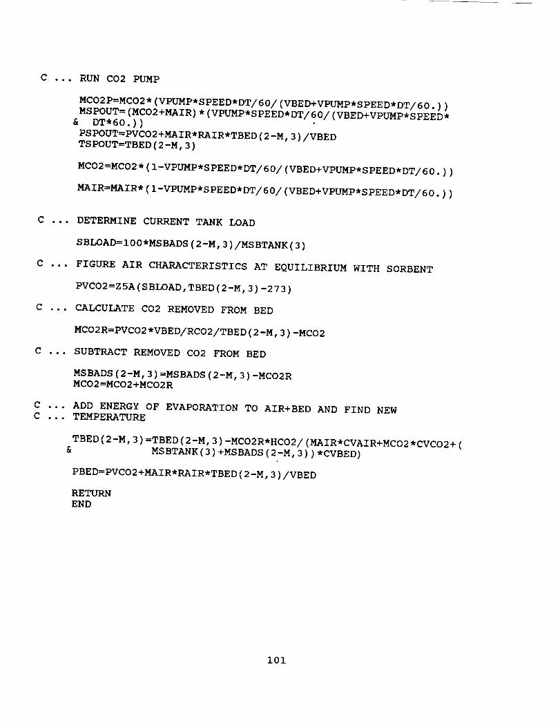
C ... RUN CO2 PUMP

MCO2P=MCO2*(VPUMP*SPEED*DT/60/(VBED+VPUMP*SPEED*DT/60.))

MSPOUT=(MCO2+MAIR)*(VPUMP*SPEED*DT/60/(VBED+VPUMP*SPEED*

& DT*60.))PSPOUT=PVCO2+MAIR*RAIR*TBED(2-M,3)/VBED

TSPOUT=TBED(2-M,3)

MCO2=MCO2*(I-VPUMP*SPEED*DT/60/(VBED+VPUMP*SPEED*DT/60.))

MAIR=MAIR*(I-VPUMP*SPEED*DT/60/(VBED+VPUMP*SPEED*DT/60.))

C ... DETERMINE CURRENT TANK LOAD

SBLOAD=I00*MSBADS(2-M,3)/MSBTANK(3)

C ... FIGURE AIR CHARACTERISTICS AT EQUILIBRIUM WITH SORBENT

PVCO2=Z5A(SBLOAD,TBED(2-M,3)-273)

C ... CALCULATE CO2 REMOVED FROM BED

MCO2R=PVCO2*VBED/RCO2/TBED(2-M,3)-MC02

C ... SUBTRACT REMOVED CO2 FROM BED

MSBADS(2-M,3)=MSBADS(2-M,3)-MCO2R

MCO2=MCO2+MCO2R

C ... ADD ENERGY OF EVAPORATION TO AIR+BED AND FIND NEW

C ... TEMPERATURE

TBED(2-M,3)=TBED(2-M,3)-MCO2R*HCO2/(MAIR*CVAIR+MCO2*CVC02+(

& MSBTANK(3)+MSBADS(2-M,3))*CVBED)

PBED=PVCO2+MAIR*RAIR*TBED(2-M,3)/VBED

RETURN

END

i01

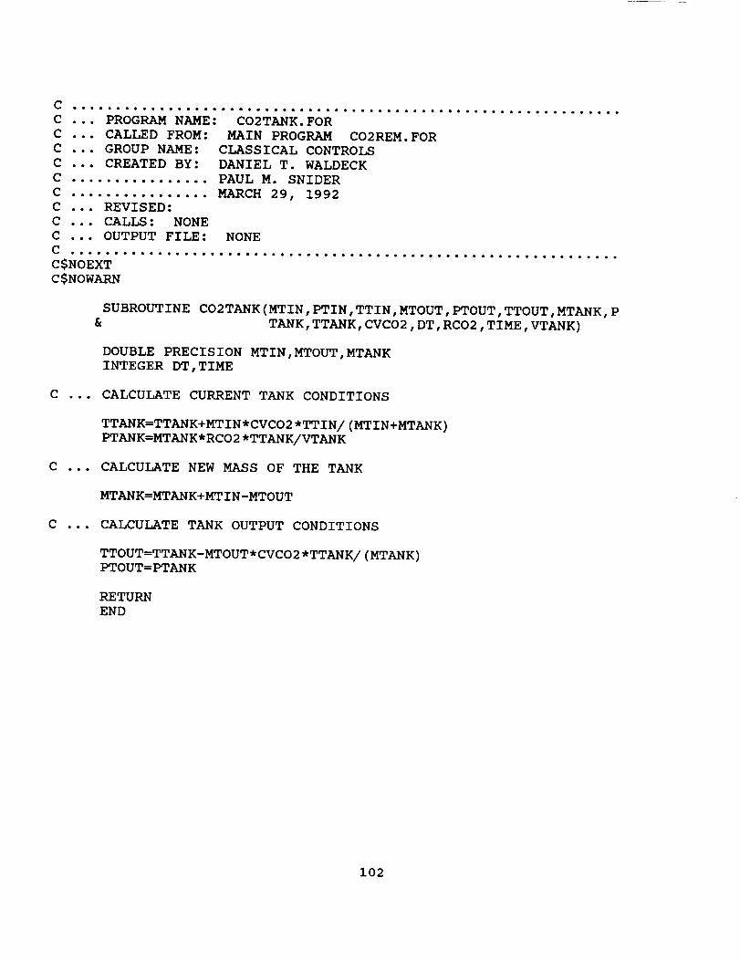
PROGRAMNAME:CALLED FROM:GROUPNAME:CREATEDBY:lallao.oo.oo

..ol.oo.m*el

REVISED:

CALLS: NONE

OUTPUT FILE:

C CLASSICAL CONTROLS

C DANIEL T. WALDECK

C PAUL M. SNIDER

C MARCH 29, 1992

C

C

C

SUBROUTINE C02TANK(MTIN,PTIN,TTIN,MTOUT,PTOUT,TTOUT,MTANK,P

& TANK,TTANK,CVCO2,DT,RCO2,TIME,VTANK)

DOUBLE PRECISION MTIN,MTOUT,MTANK

INTEGER DT,TIME

C ... CALCULATE CURRENT TANK CONDITIONS

TTANK=TTANK+MTIN*CVCO2*TTIN/(MTIN+MTANK)

PTANK=MTANK*RCO2*TTANK/VTANK

C ... CALCULATE NEW MASS OF THE TANK

MTANK=MTANK+MTIN-MTOUT

C ... CALCULATE TANK OUTPUT CONDITIONS

TTOUT=TTANK-MTOUT*CVCO2*TTANK/(MTANK)

PTOUT=PTANK

RETURN

END

102

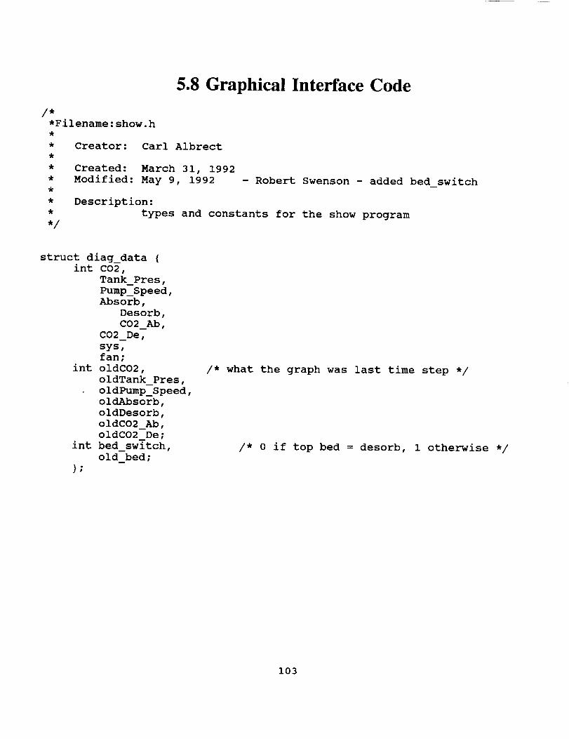
5.8 Graphical Interface Code

/*

*Filename:show.h

*/

Creator: Carl Albrect

Created: March 31, 1992

Modified: May 9, 1992 - Robert Swenson - added bed_switch

Description:

types and constants for the show program

struct diag_data {

int CO2,

Tank Pres,D

Pump_Speed,

Absorb,

Desorb,

CO2 Ab,

C02 De,

sys,

fan;

int oldCO2,

oldTank_Pres,

oldPump_Speed,

oldAbsorb,

oldDesorb,

oldCO2_Ab,oldCO2 De;

int bed_switch,

old bed;

);

/* what the graph was last time step */

/* 0 if top bed = desorb, 1 otherwise */

103

/*\

\*/

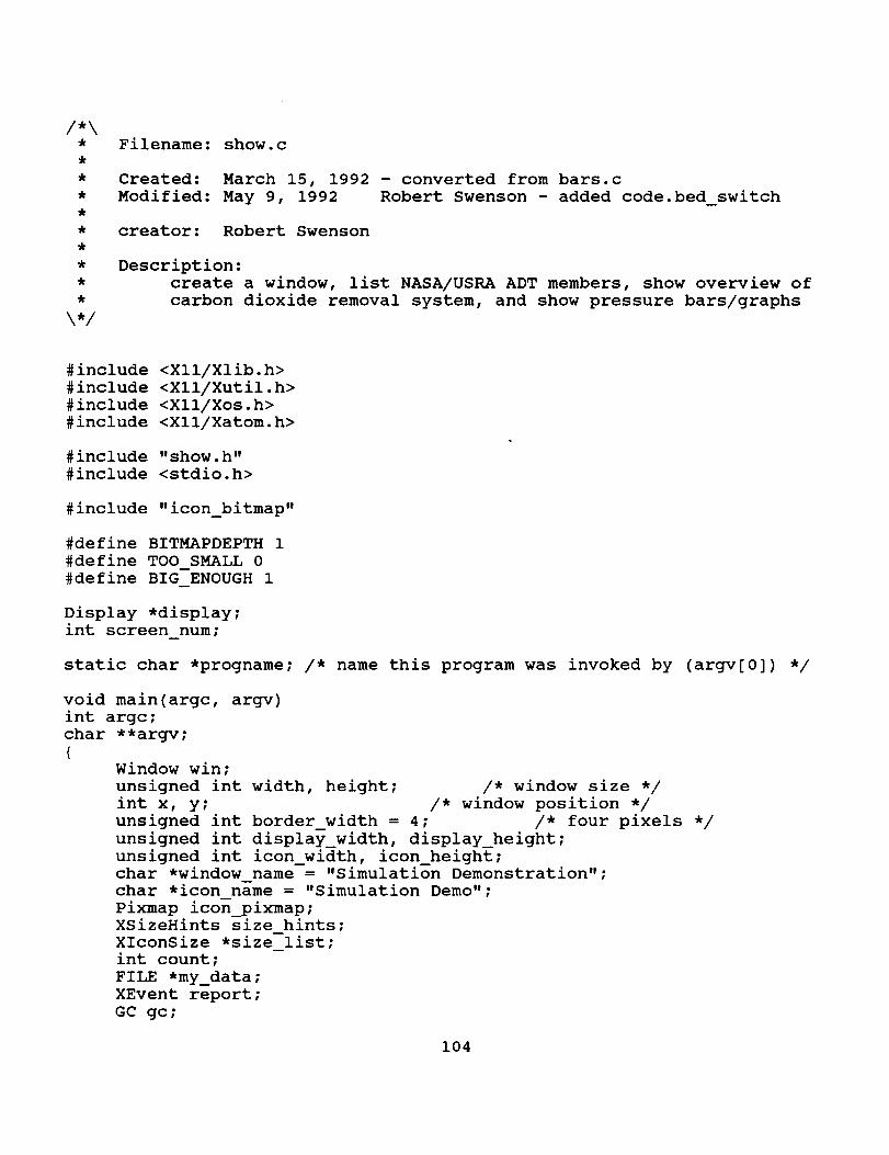
Filename: show.c

Created: March 15, 1992 - converted from bars.c

Modified: May 9, 1992 Robert Swenson - added code.bed_switch

creator: Robert Swenson

Description:

create a window, list NASA/USRA ADT members, show overview of

carbon dioxide removal system, and show pressure bars/graphs

#include <Xll/Xlib.h>

#include <Xll/Xutil.h>

#include <Xll/Xos.h>

#include <Xll/Xatom.h>

#include "show.h"

#include <stdio.h>

#include "icon_bitmap"

#define BITMAPDEPTH 1

#define TOO SMALL 0

#define BIG ENOUGH 1

Display *display;

int screen_num;

static char *progname; /* name this program was invoked by (argv[0]) */

void main(argc, argv)

int argc;

char **argv;

(Window win;

unsigned int width, height; /* window size */

int x, y; /* window position */

unsigned int border width = 4; /* four pixels */

unsigned int display_width, display_height;

unsigned int icon_width, icon_height;

char *window name = "Simulation Demonstration";

char *icon name = "Simulation Demo";

Pixmap icon_pixmap;XSizeHints size hints;

XIconSize *size_list;

int count;

FILE *my_data;

XEvent report;

GC gc;

104

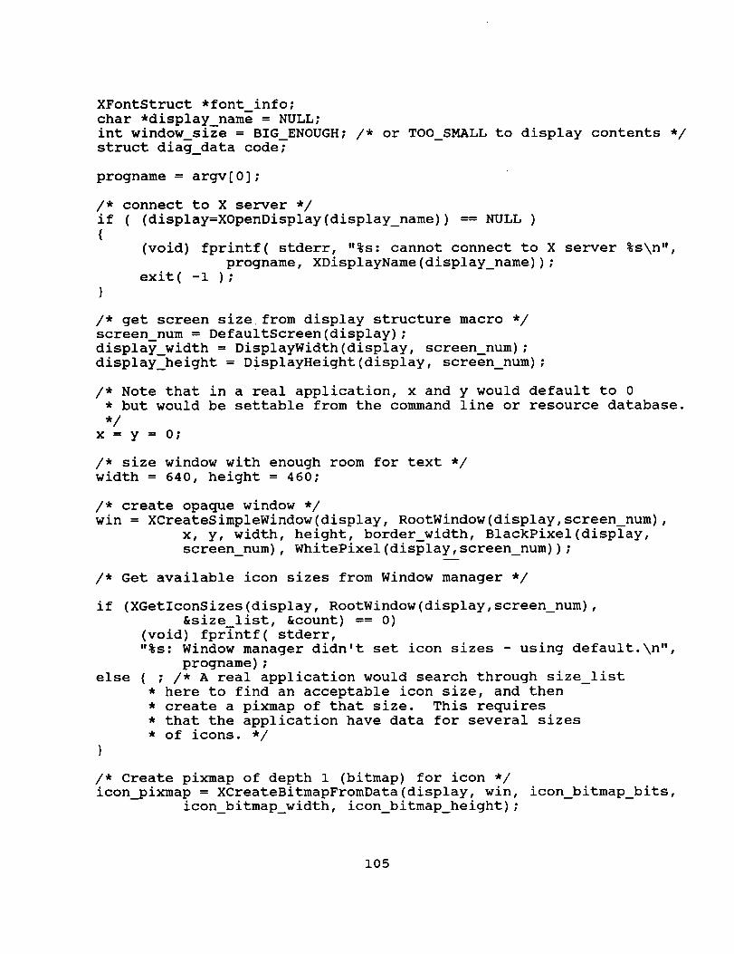
XFontStruct *font info;char *display_name = NULL;int window_size = BIG_ENOUGH; /* or TOO_SMALL to display contents */

struct diag_data code;

progname = argv[0];

/* connect to X server */

if ( (display=XOpenDisplay(display_name)) == NULL )

((void) fprintf( stderr, "%s: cannot connect to X server %s\n",

progname, XDisplayName(display_name));

exit( -I );

)

/* get screen size from display structure macro */

screen num= DefaultScreen(display);

display_width = DisplayWidth(display, screen_num);

display_height = DisplayHeight(display, screen_num);

/* Note that in a real application, x and y would default to 0* but would be settable from the command line or resource database.

*/x = y = 0;

/* size window with enough room for text */

width = 640, height = 460;

/* create opaque window */

win = XCreateSimpleWindow(display, RootWindow(display,screen_num),

x, y, width, height, border_width, BlackPixel(display,

screen_num), WhitePixel(display,screen_num));

/* Get available icon sizes from Window manager */

if (XGetIconSizes(display, RootWindow(display,screen_num),

&size_list, &count) == 0)

(void) fprintf( stderr,

"%s: Window manager didn't set icon sizes - using default.kn",

progname);

else ( ; /* A real application would search through size_list

* here to find an acceptable icon size, and then

* create a pixmap of that size. This requires

* that the application have data for several sizes

* of icons. */

/* Create pixmap of depth 1 (bitmap) for icon */

icon_pixmap = XCreateBitmapFromData(display, win, icon_bitmap_bits,

icon_bitmap_width, icon_bitmap_height);

105

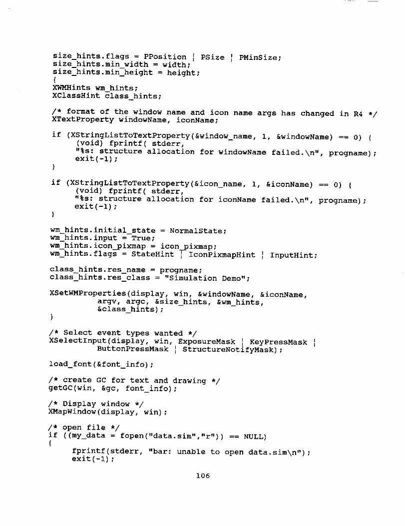
size_hints.flags = PPosition I PSize I PMinSize;size hints.min width = width;

size_hints.min_height = height;

{XWMHints wm_hints;

XClassHint class hints;

/* format of the window name and icon name args has changed in R4 */

XTextProperty windowName, iconName;

if (XStringListToTextProperty(&window_name, i, &windowName) == 0) (

(void) fprintf( stderr,

"%s: structure allocation for windowName failed.\n", progname);

exit(-l);

)

if (XStringListToTextProperty(&icon_name, i, &iconName) == 0) {

(void) fprintf( stderr,

"%s: structure allocation for iconName failed. \n", progname) ;

exit (-i) ;

)

wm hints.initial state = NormalState;

wm hints.input = True;

wm_hints.icon_pixmap = icon_ixmap;wm_hints flags = StateHint i IconPixmapHint I InputHint;

class hints.res name = progname;

class hints.res class = "Simulation Demo";

XSetWMProperties(display, win, &windowName, &iconName,

argv, argc, &size_hints, &wm_hints,

&class_hints);

)

/* Select event types wanted */I

XSelectInput(display, win, ExposureMask I KeyPressMask i

ButtonPressMask I StructureNotifyMask);

load_font (&font_info) ;

/* create GC for text and drawing */

getGC(win, &gc, font_info);

/* Display window */

XMapWindow(display, win);

/* open file */

if ( (my_data = fopen("data, sim","r") ) == NULL)

{fprintf(stderr, "bar: unable to open data.sim\n") ;

exit (-I) ;

106

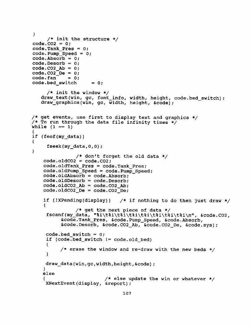
/* init the structure */code. C02 = 0;

code.Tank Pres = 0;

code. Pump_Speed = 0;

code.Absorb = 0;

code. Desorb = 0;

code.C02 Ab = 0;

code. C02 De = 0;

code.fan = 0;

code.bed switch = 0;

/* init the window */

draw text(win, gc, font info, width, height, code.bed_switch);

draw_--graphics(win, gc, width, height, &code);

/* get events, use first to display text and graphics */

/* To run through the data file infinity times */

while (i == i)

(if (feof(my_data))

{fseek(my_data, 0,0) ;

)/* don't forget the old data */

code.oldCO2 = code. C02;

code.oldTank Pres = code.Tank Pres;

code.oldPump_Speed = code. Pump_Speed;

code.oldAbsorb = code.Absorb;

code.oldDesorb =code. Desorb;

code.oldC02 Ab = code. C02 Ab;m

code.oldC02 De = code. C02 De;

if (!XPending(display)) /* if nothing to do then just draw */

{/* get the next piece of data */

fscanf(my_data, "%i\t%i\t%i\t%i\t%i\t%i\t%i\t%i\n", &code. C02,

&code.Tank_Pres, &code. Pump_Speed, &code.Absorb,

&code. Desorb, &code.CO2_Ab, &code. CO2_De, &code.sys);

code.bed switch = 0;

if (code.bed_switch != code.old_bed)

(/* erase the window and re-draw with the new beds */

}

draw_data(win,gc,width,height,&code) ;

)else

( /* else update the win or whatever */

XNextEvent(display, &report);

107

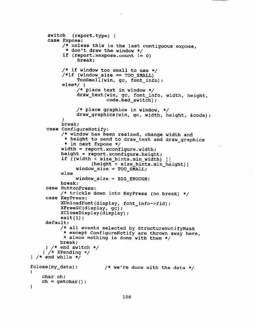
switch (report.type) (case Expose:

/* unless this is the last contiguous expose,

* don't draw the window */

if (report.xexpose.count != 0)

break;

/* if window too small to use */

/*if (window_size == TOO_SMALL)

TooSmall(win, gc, font_info);

else*/ (

/* place text in window */

draw text(win, gc, font info, width, height,

- code.bed_switCh);

/* place graphics in window, */

draw_graphics(win, gc, width, height, &code);

)break;

case ConfigureNotify:

/* window has been resized, change width and

* height to send to draw_text and draw_graphics

* in next Expose */

width = report.xconfigure.width;

height = report.xconfigure.height;

if ((width < size hints min width) II• _ II(height < size_hints.min height))

window_size = TOO SMALL;

else

window size = BIG ENOUGH;

break;

case ButtonPress:

/* trickle down into KeyPress (no break) */

case KeyPress:

XUnloadFont(display, font_info->fid);

XFreeGC(display, gc) ;

XCloseDisplay(display);

exit(l);

default:

/* all events selected by StructureNotifyMask

* except ConfigureNotify are thrown away here,

* since nothing is done with them */

break;

) /* end switch */

) /* XPending */

} /* end while */

fclose(my_data);

(char ch;

ch = getchar();

}

/* we're done with the data */

108

} /* main */

getGC(win, gc, font_info)Window win;

GC *gc;

XFontStruct *font_info;

(

unsigned long valuemask = 0; /* ignore XGCvalues and use defaults */XGCValues values;

unsigned int line width = 3;

int line_style = LineSolid;

int cap_style = CapRound;

int join_style = JoinRound;

int dash offset = 0;

static char dash_list[] = (12, 24};

int list_length = 2;

/* Create default Graphics Context */

*gc = XCreateGC(display, win, valuemask, &values);

/* specify font */

XSetFont(display, *gc, font_info->fid);

/* specify black foreground since default window background is

* white and default foreground is undefined. */

XSetForeground(display, *gc, BlackPixel(display,screen_num));

/* set line attributes */

XSetLineAttributes(display, *gc, line_width, line_style,

cap_style, join_style);

) /* getSC */

load font(font_info)

XFontStruct **font_info;

(char *fontname = "9x15";

/* Load font and get font information structure. */

if ( (*font_info = XLoadQueryFont (display, fontname) ) == NULL)

(

(void) fprintf(stderr, "%s: Cannot open 9x15 font\n",progname) ;exit ( -i ) ;

)

) /* load_font */

TooSmall(win, gc, font_info)Window win;

109

GC gc;XFontStruct *font info;

m

{char *stringl = "Too Small";

int y_offset, x_offset;

y_offset = font_info->ascent + 2;

x offset = 2;

/* output text, centered on each line */

XDrawString(display, win, gc, x_offset, y_offset, stringl,

strlen(stringl));

) /* TooSmall */

ii0

/*\

\*/

Filename: draw.c

Created: March 15, 1992 - converted from bars.c

creator: Carl Albrecht

Modified: Robert Swenson - April 3, 1992 - added draw data

Modified: RAS - May 6 - reduced window/drawing size to fit on PC

Description:Draw in the window

#include <Xll/Xlib.h>

#include <Xll/Xutil.h>

#include <Xll/Xos.h>

#include <Xll/Xatom.h>

#include <stdio.h>

#include "show.h"

extern Display *display;

#define NumStrings 30

#define TextBarWidth

*/#define TextTab

#define VOffset

#define StatBox

#define StatBarTitles

#define NumSegments 70

#define WordsInPic 25

/* number of strings to print on the screen */

280 /* width in pixels of region containing text

9 /* # of pixels to tab over for uncentered */

i0 /* move down x pixels before typing */

225 /* y Coord of the Cabin Status box */

420 /* "base" of status bars */

/* # of unconnected lines to draw */

/* # of words to print into the picture */

#define BarGraphMaxHeight I00

#define num beds 4 /* num of names to switch when beds switch */

draw_text(win, gc, font info, win_width, win_height, bed_flag)Window win;

GC gc;

XFontStruct *font info;

unsigned int win_width, win_height;

int bed_flag;

{static char *strings[NumStrings] = {

"NASA/USRA" ,

"ADT",

"at",

"Kansas State University",

"Carl Albrecht Roger Buries",

"Dan Waldeck Stan Kroeker",

iii

"Maury Wilmoth"Mike Honas","Mike Brockway"Paul Snider"Robert Swenson

Tim Sprecker",

Dr. Cogley",

Dr. Gustafson",

Robert Young",

"Cabin Status Panel",

"Carbon Tank Fan",

"Dioxide Press Speed",

"Fan",

"Dryer",

"Pump",

I

"Desorb",

"Tank",

"Pre",

"Cooler", /*22*/

"CO",

"2" , /*24*/

"Rehumidi f ier",

"Absorb", /*26*/

"Storage"

);

/'14"/

1"16"1

/.18./

/*2o*/

/* words in picture */

static struct coords { /* to make drawing the picture easier */

/* lets have an array of coordinates and */

/* strings[] indexes and just run through */

/* the array printing the words */

int x, /* coord to put the word at */

Y,the word; /* which strings[] to put at x,y */

} the_coords[WordsInPic] = 4

4410,320,14},

{560,i00,16},

(545,240,23),

4565,245,24},

(545,355,23},

(565,360,24},

4465,145,20},

4470,335,21},

(460,350,22},

4470,105,23},

{490,Ii0,24),

{455,125,27}

},bed_coords[2][num_beds] = 4 4 /* words to change when the */

/* beds switch [2] states */

(320,240,15),

4545,260,19}, /* Desorb */

(545,375,26), /* Adsorb */

4295,450,25)

112

int i;int len;int width;

I

((320,240,25),

(545,260,26),

(545,375,19),

(295,450,15)

));

int font_height = font_info->ascent + font_info->descent;

*/

for (i=0;i<4;i++) /* CENTER THE TITLES */

(len = strlen(strings[i]); /* len for XTextWidth and XDrawString */

width=XTextWidth(font_info,strings[i],len);/* str width for centering

XDrawString(display, win, gc, (TextBarWidth - width)/2,

VOffset + (i + i) * (i + font_height), strings[i], len) ;

)

for (i=4;i<ll; i++) /* SHOW THE NAMES */

{len = strlen(strings[i]); /* len for XTextWidth and XDrawString */

XDrawString(display, win, gc, TextTab,

VOffset + (i + 2) * (i + font_height), strings[i], len) ;

)

/* SHOW CABIN STATUS TITLE */

len = strlen(strings[ll]) ; /* len for XTextWidth and XDrawString */

width=XTextWidth(font_info,strings[ll],len);

XDrawString(display, win, gc, (TextBarWidth - width)/2,

StatBox + 2 * VOffset, strings[ll], len);

for (i=12;i<14;i++) /* SHOW STATUS BAR TITLES */

{len = strlen(strings[i]); /* len for XTextWidth and XDrawString */

XDrawString(display, win, gc, TextTab,

StatBarTitles + (i - ii) * (i + font_height),

strings[i], len);

)for(i=0;i<WordsInPic;i++) /* PUT WORDS IN THE PICTURE */

(len = strlen(strings[the_coords[i].the_word]);

width=XTextWidth(font info,strings[the coords[i].the_word],len);

XDrawString(display, win, gc, the coords[i].x,

the coords[i].y, strings[the_coords[i].the_word], len);

)

for(i=0;i<num_beds;i++) /* PUT IN THE bed names */

113

(len = strlen(strings[bed_coords[bed_flag][i].the_word]);

width=XTextWidth(font_info,strings[bed coords[bed_flag][i].the_word],

len);

/* INCASE the beds just switched, clear the area where this */

/* word is about to go to avoid overwrite */

/* XClearArea(); */

XDrawString(display, win, gc, bed_coords[bed_flag][i].x,

bed_coords[bed flag][i].y,

strings[bed_coords[bed_flag][i].the_word],len);

)) /* draw_text */

#define x_CO2 60 /* x coord of CO2 tank bar graph */

#define x tank 120 /* x coord of CO2 tank pres bar graph */

#define x_rpm 195 /* x coord of pump rpm bar graph */

#define x des 322 /* x coord of Deisecant bed box in diagram */

#define x_fan 411 /* x coord of the fan */

#define x_pre 460 /* X coord of precooler */

#define x CO2des 550 /* x coord of Zeolite beds */

#define BarWidth i0 /* width of status bars */

#define BoxWidth 47 /* width of the diagrams boxes */#define C Width 28 /* width of the fan circle */

#define C_Height 28 /* height of the fan circle */

#define Boxheight 53 /* height of boxes in pixels */

#define y_box 2

#define y rpm 0

#define y_pres 1

draw_graphics(win, gc, window_width, window_height, code)Window win;

GC gc;

unsigned int window_width, window_height;

struct diag_data *code;

(int x, y, oldy[3];

int height;

int width;

FILE *my_data;

int i, j, Time_Step, rpm;

float Pres;

static XSegment segments[NumSegments] = (

( 0, StatBox, TextBarWidth, StatBox},

{ TextBarWidth, 0, TextBarWidth, 0},

{ 0, StatBarTitles, TextBarWidth, StatBarTitles},

114

{ 280,190,320,190), /* pipe A top */

{ 280,200,320,200}, /* A Bottom */

{ 280,400,320,400}, /* B Top */

{ 280,410,320,410), /* B Bot */

(370,180,550,180), /* G Top */

( 370,190,550,190}, /* G Bot */

(370,200,400,200), /* D Top */

{ 370,210,390,210), /* D Bot */

(370,390,390,390), /* C Top */

(370,400,400,400), /* C Bot */

{ 370,410,550,410), /* H Top */

(370,420,550,420), /* H Bot */

{ 390,210,390,390}, /* E left */

{ 400,200,400,280), /* E Right Top */

{ 400,400,400,290), /* E Right Bot */

(400,280,410,280), /* F Top */

{ 400,290,410,290), /* F Bot */

{ 440,280,460,280}, /* I Top */

( 440,290,460,290}, /* I Bot */

{ 510,280,520,280), /* J Top */

{ 510,290,520,290), /* J Bot */

{ 520,280,520,200}, /* K Top Left */

{ 520,290,520,400), /* K Bot Left */

{ 520,200,550,200}, /* L Top */

(520,400,550,400), /* M Bot */

(530,210,530,390), /* K Right */

{ 530,210,550,210}, /* L Bot */

(530,390,550,390), /* M Top */

( 600,200,610,200}, /* N Bot */

{ 600,190,610,190), /* N Top */

(600,410,620,410), /* O Bot */

{ 600,400,610,400), /* 0 Top */

(610,400,610,200), /* P Bot Left */

{ 425,270,425,300}, /* Fan blades */

{ 410,285,440,285), /* Fan Blades */

{ 416,275,435,295}, /* Fan Blades */

{ 416,295,435,275), /* Fan Blades */

(610,190,610,80), /* P Top Left */

{ 620,410,620,70),

( 610,80,580,80),

( 620,70,590,70),

{ 560,60,510,60),

{ 570,50,510,50),

( 450,60,370,60),

{ 450,50,370,50),

{ 370,40,370,70),

( 300,40,300,70},

{ 350,20,320,20},

{ 350,90,320,90),

( 370,40,350,20),

{ 370,70,350,90},

/* P Right */

/* Q Bot */

/* Q Top */

/* R Bot */

/* R Top */

/* S Bot */

/* S Top */

/* Draws the octagon/OGA */

/* Draws the octagon/OGA */

/* Draws the octagon/OGA */

/* Draws the octagon/OGA */

/* Draws the octagon/OGA */

/* Draws the octagon/OGA */

115

};

{ 300,40,320,20}, /* Draws the octagon/OGA */

( 300,70,320,90}, /* Draws the octagon/OGA */

( 565,55,570,60}, /*Draws the pumps*/

{ 585,75,580,70}, /* Draws the pump */

{ 460,250,480,280},/*Draws the PreCooler*/

{ 480,280,485,270},

{ 485,270,490,280},

( 460,330,480,300},

{ 480,300,485,310},

{ 485,310,490,300},

( 490,300,510,330},

{ 490,280,510,250}

segments[l].y2 = window_height; /* window height is a var so it

can't

be used in the aggragrate assignment */

./

/* draw the picture */

XDrawSegments(display, win, gc, segments, NumSegments); /* draw pipes

XDrawRectangle(display,win,gc,x_des,170,47,Boxheight); /* AA */

XDrawRectangle(display,win,gc,x_des,380,47,Boxheight); /* BB */

XDrawRectangle(display,win,gc,x_pre,260,50,Boxheight); /* EE */

XDrawRectangle(display,win,gc,x_CO2des,170,50,Boxheight);/* CC */

XDrawRectangle(display,win,gc,x_CO2des,380,50,Boxheight);/* DD */

/* This draws the fan */

XDrawArc(display,win,gc,410,270,30,30,0,360 * 64);

/* This draws the pump */

XDrawArc(display,win,gc,560,50,30,30,0,360 * 64);

/* This draws the center of the pump */

XDrawArc(display,win,gc,570,60,10,10,0,360 * 64);

/* This draws the CO2 Storage Tank */

XDrawArc(display,win,gc,450,25,60,60,0,360 * 64);

,//* When drawing/redrawing the whole pic, draw complete level bars

/* instead of just the changed part */

code->oldCO2 = 0;

code->oldTank Pres = 0;

code->oldPump_Speed = 0;code->oldAbsorb = 0;

code->oldDesorb = 0;

code->oldCO2 Ab = 0;

code->oldC02 De = 0;

draw data(win,gc,width,height,code,y);

} /* draw_graphics */

116

draw data(win,gc,width,height,code,y)Window win;GC gc;int width;int height;struct diag_data *code;int y;{

/* draw the moving bars */

if (code->CO2 > BarGraphMaxHeight)

code->CO2 = BarGraphMaxHeight;

height = BarGraphMaxHeight - code->C02;

XClearArea(display, win, x_CO2, StatBarTitles - BarGraphMaxHeight,

BarWidth, height, 0) ;

y = StatBarTitles - code->C02;

height = code->CO2;XFillRectangle(display, win, gc, x_C02, y, BarWidth, height);

if (code->Tank_Pres > BarGraphMaxHeight)

code->Tank_Pres = BarGraphMaxHeight;

XClearArea(display, win, x_tank, StatBarTitles -

BarGraphMaxHeight,BarWidth, BarGraphMaxHeight - code->Tank_Pres, 0);

y = StatBarTitles - code->Tank_Pres;

height = code->Tank Pres;

XFillRectangle(disp[ay, win, gc, x_tank, y, BarWidth, height);

if (code->Pump_Speed > BarGraphMaxHeight)

code->Pump_Speed = BarGraphMaxHeight;

XClearArea(display, win, x_rpm, StatBarTitles - BarGraphMaxHeight,

BarWidth, BarGraphMaxHeight - code->Pump_Speed, 0);

y = StatBarTitles - code->Pump_Speed;

height = code->Pump Speed;XFillRectangle(disp[ay, win, gc, x_rpm, y, BarWidth, height);

/* draw the box fillings */

if (code->Absorb > code->oldAbsorb)

{

117

y = 222 - code->Absorb;

height = code->Absorb- code->oldAbsorb;

XFillRectangle(display, win, gc, x des+2, y, BoxWidth, height);)

else if (code->Absorb < code->oldAbsorb){

y = 222 - code->oldAbsorb;

height = code->oldAbsorb - code->Absorb;

XClearArea(display, win, x_des+2, y, BoxWidth-2,height,0);)

if (code->Desorb > code->oldDesorb)(y = 432 - code->Desorb;

height = code->Desorb - code->oldDesorb;

XFillRectangle(display, win, gc, x des+2, y, BoxWidth, height);)

else if (code->Desorb < code->oldDesorb)(

y = 432 - code->oldDesorb;

height = code->oldDesorb - code->Desorb;

XClearArea(display, win, x des+2, y, BoxWidth-2, height,O);)

if (code->CO2_Ab > code->oldCO2_Ab){y = 222 - code->CO2 Ab;

height = code->C02 Ab - code->oldCO2 Ab;

XFillRectangle(display, win, gc, x_CO2des+2, y, BoxWidth, height);)

else if (code->CO2_Ab < code->oldCO2_Ab){

y = 222 - code->oldCO2_Ab;height = code->oldCO2 Ab - code->CO2 Ab;

XClearArea(display, wln, x CO2des+2, y, BoxWidth, height,0);)

if (code->CO2_De > code->oldCO2_De)(y = 432 - code->CO2 De;

height = code->CO2 De - code->oldCO2_De;

XFillRectangle(display, win, gc, x CO2des+2, y, BoxWidth, height);)

else if (code->CO2_De < code->oldCO2 De)(

y = 432 - code->oldCO2_De;

height = code->oldCO2 De - code->CO2 De;

XClearArea(display, _wln, x_CO2des+2, y, BoxWidth, height,0);)

/* draw the fan moving */

118

if (code->sys == I)

(XClearArea(display, win, x_fan, 271, C_Width, C Height,O);

XDrawArc(display,win,gc,410,270,30,30,0,360 * 64);

XDrawLine(display,win,gc,425,270,425,300);

XDrawLine(display,win,gc,410,285,440,285);

XDrawLine(display,win,gc,416,275,435,295);

XDrawLine(display,win,gc,416,295,435,275);

)) /* draw_data */

119