Embed Size (px)
Citation preview

Automation of Quantity Takeoff and Material Optimization for Residential
Construction Manufacturing
By
Hongru Zhao
A thesis submitted in partial fulfillment of the requirements for the degree of
Master of Science
In
Construction Engineering and Management
Department of Civil and Environmental Engineering
University of Alberta
©Hongru Zhao, 2015
ii
Abstract
Quantity takeoff is repetitive work in the modular construction industry. The
current process, which is typically carried out manually, is time consuming and
error-prone. This thesis proposes a methodology to automate the quantity takeoff
process. The central aim of this research is to create a bridge between the building
information modelling (BIM) 3D model and a database that can be used to hold
data extracted from the model. This bridge allows the automatic transfer of
material quantities from the BIM model to the database. Another issue associated
with residential construction is material waste, especially for 1D and 2D framing
materials, which is caused by insufficient planning of cutting processes. Hence,
this thesis also presents a methodology to optimize material usage (focusing on
lumber and sheathing). 1D and 2D materials are extracted from the BIM 3D
model and then organized in order to establish optimized lumber and sheathing
cutting plans.

iii
Table of Contents
Chapter 1 Introduction ............................................................................................ 1
1.1 Research Motivation ................................................................................................. 1
1.2 Research Objectives .................................................................................................. 3
1.3 Thesis Organization .................................................................................................. 4
Chapter 2 Literature Review ................................................................................... 6
2.1 Introduction ............................................................................................................... 6
2.2 Building Information Modelling ............................................................................... 6
2.3 Quantity Takeoff ....................................................................................................... 7
2.4 Material Optimization ............................................................................................... 8
Chapter 3 Proposed Methodology ........................................................................ 12
3.1 Quantity takeoff ...................................................................................................... 12
3.1.1 Preloading the BIM model with a unique classification system ...................... 13
3.1.2 Quantification Measurement ............................................................................ 14
3.1.2 Format database template ................................................................................. 14
3.1.3 Quantity Extraction .......................................................................................... 21
3.2 Material Optimization ............................................................................................. 22
3.2.1 Lumber Optimization ....................................................................................... 22
3.2.2 Sheathing Optimization .................................................................................... 33
3.2.3 Sheathing Optimization .................................................................................... 56
Chapter 4 Case Study ............................................................................................ 68
4.1 Introduction ............................................................................................................. 68
4.2 Quantity Takeoff ..................................................................................................... 68
4.2.1 Background ...................................................................................................... 68
4.2.2 Preloading the Revit Model ............................................................................. 69
4.2.3 Standardization of Excel Template .................................................................. 70
4.2.4 Quantity Extraction .......................................................................................... 71
4.3 Material Optimization ............................................................................................. 74
4.3.1 Background ...................................................................................................... 74
4.3.2 Lumber Optimization ....................................................................................... 76
iv
4.3.3 Sheathing Placement and Optimization ........................................................... 98
Chapter 5 Conclusion .......................................................................................... 117
5.1 General Conclusion ............................................................................................... 117
5.2 Research Contributions ......................................................................................... 118
5.2.1 Quantity Takeoff ............................................................................................ 118
5.2.2 Material Optimization .................................................................................... 118
5.3 Research Limitations............................................................................................. 119
5.4 Future Improvement .............................................................................................. 120
References ........................................................................................................... 121
Appendices .......................................................................................................... 124

v
Table of Figures
Figure 1.1: Construction waste on site (Waste Management World 2014). ....................... 3
Figure 2.1: Material waste from framing (by volume) (Mah 2008).................................... 9
Figure 3.1: Overview of methodology of quantity takeoff. .............................................. 13
Figure 3.2: Material category classification. ..................................................................... 14
Figure 3.3: Decomposition of wall materials. ................................................................... 16
Figure 3.4: House wrap membrane installation (Insulation-Online 2014). ....................... 18
Figure 3.5: Insulation installation between two studs (“Basement Wall Insulation Blanket
- Viewing Gallery” 2014). ................................................................................................ 19
Figure 3.6: Database property structure. ........................................................................... 21
Figure 3.7: Examples of dimensional lumber, regular length, and lumber pieces (Pekin
Hardwood 2015; Build Your Own House 2011). ............................................................. 23
Figure 3.8: Overview of methodology of lumber optimization. ....................................... 24
Figure 3.9: Virtual lumber pool (2x6). .............................................................................. 25
Figure 3.10: Flowchart of lumber cutting process. ........................................................... 26
Figure 3.11: Grouped lumber pool (2x6). ......................................................................... 28
Figure 3.12: Tree structure. ............................................................................................... 29
Figure 3.13: Overview of methodology of material optimization. ................................... 35
Figure 3.14: Revit family—sheathing. .............................................................................. 36
Figure 3.15: A 3D object can be located by one point and two vectors. ........................... 37
Figure 3.16: Wall direction decided by drawing direction. .............................................. 38
Figure 3.17: Two possible Framing Points of a wall framing. .......................................... 39
Figure 3.18: Butt wall joint type. ...................................................................................... 40
Figure 3.19: Modify Butt wall joint to Miter. ................................................................... 40
Figure 3.20: Overlap of wall and wall framing (Framing Points are identical and circled
in red). ............................................................................................................................... 41
Figure 3.21: Top view of the overlap of wall and wall framing (Framing Point circled in
red). ................................................................................................................................... 42
Figure 3.22: Highlight of wall bottom corner. .................................................................. 43
Figure 3.23: Wall layers with thicknesses. ....................................................................... 43
Figure 3.24: Components and dimensions of wall framing. ............................................. 44
Figure 3.25: Height determination rule (window and door). ............................................ 46
Figure 3.26: Height determination rule (sheathing height is higher than wall height). .... 46
vi
Figure 3.27: Height determination rule (sheathing height is lower than wall height). ...... 47
Figure 3.28: Stud categories.............................................................................................. 48
Figure 3.29: Highlight of SJOIN studs. ............................................................................ 49
Figure 3.30: Sheathing length determination. ................................................................... 50
Figure 3.31: Start Point determination (wall without window or door). ........................... 51
Figure 3.32: Start Point determination (door). .................................................................. 53
Figure 3.33: Start Point determination (window). ............................................................ 54
Figure 3.34: Start Point determination (wall height is higher than sheathing height). ...... 55
Figure 3.35: Sheathing labels. ........................................................................................... 55
Figure 3.36: NonGuillotine and Guillotine cutting pattern (Manrique et al. 2011). ......... 56
Figure 3.37: The only way to cut five small certain squares in a large square (Solving the
2D Packing Problem 2007). .............................................................................................. 58
Figure 3.38: Flowchart of sheathing cutting process. ....................................................... 59
Figure 3.39: Sheathing piece rotation. .............................................................................. 61
Figure 3.40: Regular sheathing rotation. ........................................................................... 61
Figure 3.41: Sheathing piece fits on a regular sheathing. ................................................. 62
Figure 3.42: Dimensions after fitting piece on a regular sheathing. ................................. 63
Figure 3.43: Bottom Left point moves to fit more sheathing pieces. ................................ 64
Figure 3.44: Stair shape sheathing remaining after first-round fit. .................................. 65
Figure 3.45: Three second-round rectangles. .................................................................... 65
Figure 3.46: Three possible cutting plans on a sheet of regular sheathing. ...................... 67
Figure 4.1: 3D view of case study model. ......................................................................... 69
Figure 4.2: Top view of case study model. ....................................................................... 69
Figure 4.3: Preloaded information in the Revit model. ..................................................... 70
Figure 4.4: Quantity takeoff interface (ExportToExcel). .................................................. 71
Figure 4.5: Error prompt dialog. ....................................................................................... 74
Figure 4.6: A mini home from Kent Homes. .................................................................... 75
Figure 4.7: Top view of case study model. ....................................................................... 75
Figure 4.8: Front view of case study model. ..................................................................... 75
Figure 4.9: Back view of case study model. ..................................................................... 76
Figure 4.10: Wall framing of case study model. ............................................................... 77
Figure 4.11: Stud properties. ............................................................................................. 78
Figure 4.12: Lumber pool (2x4). ....................................................................................... 80
Figure 4.13: Lumber cutting (configuration 1). ................................................................ 81

vii
Figure 4.14: Lumber cutting (configuration 2). ................................................................ 82
Figure 4.15: Lumber cutting (configuration 3). ................................................................ 82
Figure 4.16: Lumber cutting (configuration 4). ................................................................ 83
Figure 4.17: Lumber cutting (configuration 5). ................................................................ 84
Figure 4.18: Lumber optimization interface (lumber information input). ........................ 85
Figure 4.19: Wall framing layout with lumber labels (Exterior Wall AX3). .................... 98
Figure 4.20: Sheathing placement and optimization interface. ......................................... 99
Figure 4.21: Highlight of Framing Point in case study. .................................................. 100
Figure 4.22: Wall layer thicknesses in case study. .......................................................... 100
Figure 4.23: Framing Point and three possible sheathing lengths in the wall framing. .. 102
Figure 4.24: Three Start Points are created. .................................................................... 105
Figure 4.25: Sheathing placements in case study. ........................................................... 106
Figure 4.26: Sheathing placement (4x8). ........................................................................ 107
Figure 4.27: Sheathing piece to cover the upper portion of wall (1). ............................. 108
Figure 4.28: Sheathing piece to cover the upper portion of wall (2). ............................. 109
Figure 4.29: Sheathing placement (4x7). ........................................................................ 109
Figure 4.30: Sheathing piece fitting (1). ......................................................................... 111
Figure 4.31: Sheathing piece fitting (2). ......................................................................... 112
Figure 4.32: Sheathing piece fitting (3). ......................................................................... 113
Figure 4.33: Sheathing piece fitting (4). ......................................................................... 114
Figure 4.34: Sheathing piece fitting (5). ......................................................................... 114
Figure 4.35: Sheathing piece fitting (6). ......................................................................... 115
Figure 4.36: Sheathing placement and optimization interface (export cutting plans). .... 115
Figure 4.37: Sample sheathing cutting plan. ................................................................... 116

viii
List of Tables
Table 4.1: Sample of Excel template (Unit_Number assignment). ................................... 71
Table 4.2: Sample of extracted quantities. ........................................................................ 72
Table 4.3: Stud properties and naming rule. ..................................................................... 78
Table 4.4: Studs collection from case study...................................................................... 79
Table 4.5: Grouped lumber pool (2x6). ............................................................................ 85
Table 4.6: Optimized lumber cutting plan (12 ft only). .................................................... 90
Table 4.7: Optimized lumber cutting result (12 ft only). .................................................. 91
Table 4.8: Optimized lumber cutting plan (10 ft only). .................................................... 92
Table 4.9: Optimized lumber cutting result (10 ft only). .................................................. 93
Table 4.10: Optimized lumber cutting plan (8 ft only). .................................................... 94
Table 4.11: Optimized lumber cutting result (8 ft only). .................................................. 95
Table 4.12: Optimized lumber cutting plan (mixed). ........................................................ 96
Table 4.13: Optimized lumber cutting result (mixed). ...................................................... 97
Table 4.14: Sheathing pieces. ......................................................................................... 110

ix
List of Abbreviations
BIM: Building Information Modelling
1D: One-dimensional
2D: Two-dimensional
3D: Three-dimensional
OSB: Oriented Strand Board
GA: Genetic Algorithms
ACO: Ant Colony Optimization
C1: Category 1
C2: Category 2
C3: Category 3
1
Chapter 1 Introduction
1.1 Research Motivation
Quantity takeoff, serving as a foundation for downstream tasks in the
management of modular construction, is repetitive work. The process in current
practice involves manual interventions, which is time consuming and error-prone.
The challenge of transitioning construction companies to a better and more
efficient method is multifaceted; one challenge is incorporating a cost breakdown
structure that is formulated according to the company’s classification systems into
building information modelling (BIM). This study develops a methodology which
enables construction practitioners to obtain quantity takeoff in an automated
manner. The main concept is to preload the unique classification information into
the BIM model so that the quantity of materials in the BIM model can be
extracted and stored into a database automatically in accordance with the
preloaded classification system. The unique classification information, along with
formulas for derived material quantities, is front-loaded into the database. As a
result, the explicitly extracted quantities are converted by means of the preloaded
formulas in the database to the required format for the purpose of ordering and
purchasing materials. A prototype system is developed based on Autodesk Revit
through the Revit Application Programming Interface. A case study of the
manufacturing of a modularized house reveals that, a considerable amount of time
saving and increased accuracy for project estimation are achieved as a result of
utilizing automated quantity takeoff.

2
Another deficiency in the current residential construction process is the waste of
materials. One reason for this has been the general lack of focus on material
saving methods. From 2005 to 2008, Western Canada observed a rise in housing
costs partially due to the shortage of experienced trades personnel, which in turn
led to a relative decrease in the cost of material comparing with the cost of labour.
As such, efforts to optimize material usage in Western Canada’s construction
market have been relatively limited in recent years. As a consequence, material
has been misused, and large amounts of waste have been generated (Manrique
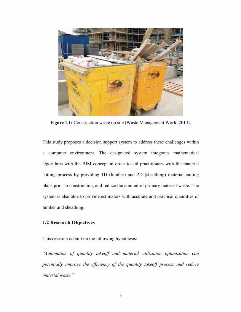
2009). Among the most highly wasted products, solid sawn wood, engineered
wood (e.g., lumber, sheathing), and drywall account for over 60% of all waste by
weight (Home Innovation Research Labs 2001) (Figure 1.1). A common cause of
waste among the aforementioned materials is the necessity of cutting these
materials on site, and the current cutting practice depends on the intuition and
guesswork of the worker (which leads to error) rather than adhering to a
comprehensive plan. In specific, the large amount of primary materials wasted can
be attributed to the lack of a predetermined cutting plan. This underscores the
distinct need for a practical methodology to optimize the use of primary materials.
3
Figure 1.1: Construction waste on site (Waste Management World 2014).
This study proposes a decision support system to address these challenges within
a computer environment. The designated system integrates mathematical
algorithms with the BIM concept in order to aid practitioners with the material
cutting process by providing 1D (lumber) and 2D (sheathing) material cutting
plans prior to construction, and reduce the amount of primary material waste. The
system is also able to provide estimators with accurate and practical quantities of
lumber and sheathing.
1.2 Research Objectives
This research is built on the following hypothesis:
“Automation of quantity takeoff and material utilization optimization can
potentially improve the efficiency of the quantity takeoff process and reduce
material waste.”

4
This research aims to improve the productivity of the modular construction
industry through two main tasks automation of quantity takeoff and material
optimization. The objectives of the research are summarized below:
• To develop a deep understanding of the current quantity takeoff process
• To front-load the information into the Revit model and database
• To obtain a precise quantity takeoff in a timely manner
• To build and implement an algorithm to minimize the material (lumber and
sheathing) waste
• To create and visualize sheathing layouts on exterior walls in the Revit
model automatically
• To provide a practical quantity of lumber and sheathing for ordering
purposes
• To report the revised material quantity quickly due to design changes.
1.3 Thesis Organization
Chapter 1 (Introduction) describes the research motivation and objectives and
provides an overview of the research.
Chapter 2 (Literature Review) provides a description of BIM application in
current construction practices, as well as a summary of state-of-the-art BIM-based
quantity takeoff and material optimization.

5
Chapter 3 (Proposed Methodology) describes the proposed methodology utilized
to perform quantity takeoff and material optimization.
Chapter 4 (Case Study) applies the developed programs to two Revit models for
demonstration.
Chapter 5 (Conclusion) summarizes the research contributions, limitations, and
future work.

6
Chapter 2 Literature Review
2.1 Introduction
In this chapter, previous and current research related to quantity takeoff and
material optimization is described.
2.2 Building Information Modelling
Building Information Modelling (BIM) is a proven, an effective technology in the
architecture, engineering, and construction (AEC) domain (Azhar 2011). The term
Building Information Modelling was introduced by van Nederveen and Tolman
(1992). BIM constitutes a 3D geometric modelling paradigm in which information
stored in a data-rich BIM model can be implemented for prediction and analysis
in different applications, such as energy consumption quantification, structural
performance, and cost, scheduling, and facilities management (Kensek 2014). One
notable characteristic of BIM is the ability to manage changes, such as design and
schedule changes, through the database stored in the BIM system (“Building
Information Modeling” 2002), and it also offers a potential capacity to share
digital resources among project participants throughout the project lifecycle
(Sabol 2008).
BIM is an emerging paradigm which is spreading quickly in the construction
industry, and a considerable number of BIM software applications have been
developed, such as Autodesk Revit, Graphisoft ArchiCAD and Vico Office Suite.

7
Most of these software applications are equipped with an application
programming interface (API) function, and the function can be broadened by
using the specialized programs written by external application developers
(Modeling 2008). Among the software, Autodesk Revit provides a rich and
powerful .NET API to perform automation of repetitive tasks and extension of the
core functionality of Revit in simulation, conceptual design, construction and
building management, as well as other functionalities (Autodesk Developer
Network 2015).
2.3 Quantity Takeoff
Quantity takeoff is an important part of the construction process, and it is
performed by general contractors, subcontractors, cost consultants, and quantity
surveyors. Such tasks simply include measuring and counting the utilization of
materials within a certain construction project in order to determine the associated
materials and total labour usage. In current practice, the quantity takeoff process
is typically carried out manually using a printout, a pen, and a calculator, which is
an outdated method (Beyond the Paper 2006). Since the process of manual
quantity takeoff depends on human interpretation, it is difficult to obtain accurate
measurements and avoid errors (Monteiro and Poças Martins 2013). The
development of BIM provides a better environment for quantity takeoff. In recent
years, an increasing number of practitioners have been adopting BIM, as it
provides a feasible means to develop a more efficient quantity takeoff system
(Firat et al. 2010). BIM enables project teams to generate cost estimates quickly
and accurately, and the output can be used to assist in material ordering and cost
8
estimation, not only early in the design phase but throughout the project lifecycle
(Autodesk 2013).
For the stick-built onsite construction practice, Autodesk has developed
commercial software called “Autodesk Quantity Takeoff”, which is widely used
by the construction industry. It enables cost estimators to read and extract
information (geometry, images, and data) from BIM tools, such as Revit
Architecture, Revit Structure, and Revit MEP. After importing the data from other
software, Autodesk Quantity Takeoff is able to automatically measure, count, and
price building objects in minutes, and the takeoff results can be exported in
different file formats such as Microsoft Excel and Design Web Format (DWF)
(Autodesk 2015); however, this tool is not designed to support modular and
offsite construction.
2.4 Material Optimization
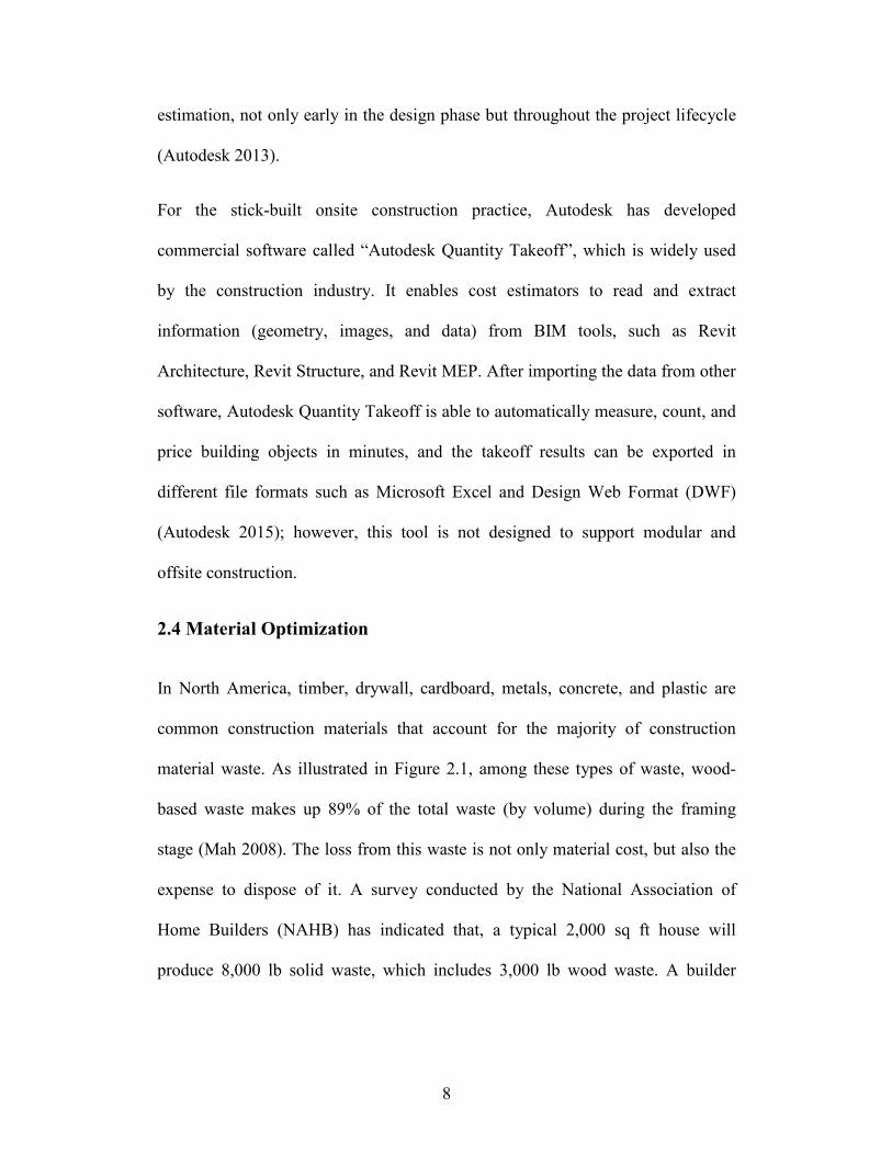
In North America, timber, drywall, cardboard, metals, concrete, and plastic are
common construction materials that account for the majority of construction
material waste. As illustrated in Figure 2.1, among these types of waste, wood-
based waste makes up 89% of the total waste (by volume) during the framing
stage (Mah 2008). The loss from this waste is not only material cost, but also the
expense to dispose of it. A survey conducted by the National Association of
Home Builders (NAHB) has indicated that, a typical 2,000 sq ft house will
produce 8,000 lb solid waste, which includes 3,000 lb wood waste. A builder
9
needs to pay over $500 for construction waste disposal for each house (Home
Innovation Research Labs 2001).
Figure 2.1: Material waste from framing (by volume) (Mah 2008).
The quantification of construction material waste has garnered significant
attention among researchers, but few studies have focused on methods to decrease
material waste beginning at the design phase (Manrique 2009). Since the majority
of waste is caused by insufficient cutting plans, it is necessary to develop an
approach to reduce wood-based waste before construction begins.
A well-known approach to optimize material usage is the coupling of
combinatorial analysis and linear programming, which began to appear in the 20th
century (Manrique 2009). In the early 1960s, Gilmore and Gomory (1961)
proposed a practical method to solve the 1D cutting stock problems. They
transformed each cutting pattern and the demand requirements to integer arrays,
and enabled the constraints to satisfy the requirements by combining different
cutting patterns. Early adaptation was challenging due to the considerable number

10
of equations and large calculation tasks; however, this has become much more
manageable with the development of complex computational software (David et
al. 2009).
Numerous individual and combinatorial optimization algorithms have been
implemented to solve 2D cutting stock problems. Genetic Algorithms (GA) and
Ant Colony Optimization (ACO) are suitable to solve constraint satisfaction and
combinatorial optimization problems. Costa and Sassi (2012) developed a
guillotine cutting process (Guillotine cutting refers to a cutting pattern for
rectangular forms where the cutting edge begins at one side and continues towards
the opposite side without stopping; it is also called edge-to-edge cutting
(Aryanezhad et al. 2012)) for the glass industry based on the combination of GA
and ACO; however, this cutting process was only sufficient for a small number of
objects. If the number of glass pieces to be cut from the same plate was increased,
the time to calculate the optimal solution would also increase in a factorial
relation. Furthermore, when the work complexity is high, the required time
necessary to complete the task becomes unacceptable. MacLeod (1993) applied an
O(n3) approximation algorithm to the 2D guillotine cutting stock problem, and the
concept of this algorithm is to locate each rectangle from a stock pile onto a
feasible position on the stock piece, and a position will only be located for a
certain rectangle if and only if such a feasible placement exists. In order to speed
up the calculation process, Manrique (2011) proposed a combinatorial algorithm
called CUTEX to amalgamate BIM and optimization. The algorithm was applied
to optimize lumber and sheathing usage to satisfy project demand as extracted

11
from Autodesk CAD drawings, and the results showed that CUTEX could reduce
wood waste from the construction of dwellings by 96%. The research presented in
this thesis is built on Manrique (2011) combining of combinatorial analysis and
linear programming utilizing advanced BIM technologies.

12
Chapter 3 Proposed Methodology
3.1 Quantity takeoff
In this chapter, the methodology of performing quantity takeoff is described.
Compared with current conventional software, the proposed program is capable of
generating quantity takeoff reports in a self-customized format, and of allowing
the user to edit formulas in the database in order to modify the extracted quantity
to a practical quantity. In addition, the proposed quantity takeoff program runs
inside the BIM software, which circumvents the processes of exporting (from
BIM software) and importing (into quantity takeoff software) models.
As the overview of the methodology in Figure 3.1 shows, the main process is to
front-load a unique material information classification system (e.g., Part Number
and Unit Number) into the BIM 3D model and database template, and to extract
the material quantity in accordance with the Part Number and Unit Number to the
database. A certain portion of directly extracted quantities are inadequate to be
utilized for inventory, and the front-loaded formulas in the database are designed
to process and classify the quantities. A detailed explanation is given in the
following sections.

13
Figure 3.1: Overview of methodology of quantity takeoff.
3.1.1 Preloading the BIM model with a unique classification system
The concept of quantity takeoff involves (1) integrating BIM software with a
company’s inventory database coherently through a unique classification system,
and (2) quantifying the items from the BIM software model into the database
template. The “bridge” used to link the two ends is Part Number, which is a
numeric identifier of an item. To extract the quantities of materials, Part Numbers
are preloaded into the BIM 3D model and assigned to each item. However, under
certain circumstances, Part Number is not sufficient to classify items for modular
construction. The nature of this construction method is such that a single project
comprises multiple independent modules. To distinguish the modules, each one is
assigned a property referred to as Unit Number, and all the materials belonging to
the same module are assigned the identical Unit Number.

14
3.1.2 Quantification Measurement
To facilitate the quantity extraction, material usage is quantified through various
measurements: each, linear length, and contact area. In this study, materials are
separated into three categories corresponding to the different measurement units
and front-loaded information to the 3D model (Figure 3.2).
Figure 3.2: Material category classification.
• Category 1 (C1): Materials counted by each (e.g., doors and windows).
• Category 2 (C2): Materials counted by linear length (e.g., lumber and
pipe).
• Category 3 (C3): Materials counted by contact area (e.g., OSB sheathing
and drywall).
3.1.2 Format database template
A standardized database template is a prerequisite to automating the quantity
takeoff. Generally, the database template contains all the necessary items for

15
construction of the module; it thus could be commonly modified from a
company’s Inventory File.
At least five properties are recorded in the database: Part Number, Description,
Unit, Module Number, and Quantity. Part Number and Module Number are the
primary and secondary indicators used to conduct the quantity extraction.
Description and Unit are supplementary properties for description of a certain
material. All the properties except Quantity are constant and front-loaded into the
database; the Quantity input is left blank to hold the quantity that will be extracted
from the BIM 3D model. In most cases, the content in the database template needs
to be duplicated a few times, and the number of duplications should be equal to
the quantity of the units (modules) within a model. After each copy of the content,
different Module Numbers are assigned. However, this database structure is still
not fully feasible for quantity takeoff due to three considerations: (1) inevitable
waste, (2) actual construction method, and (3) unit conversion.
Among the three material categories, the items in the first category (C1) do not
need any further processing after being extracted, and the quantities are regarded
as 100% accurate. For example, “five windows and four doors” are extracted from
the model, which precisely indicates that five windows and four doors are
required for the project. However, the quantities of items in the second category
(C2) have less accuracy than the first category, since the C2 materials always
realistically require extra processing work (e.g., cutting of lumber or pipe). The
third category (C3) has the lowest accuracy, since C3 materials usually necessitate
2D cuts in order to obtain suitable sizes. The additional processes of C2 and C3

16
materials cause inevitable waste, which leads to a significant deviation in quantity
estimation. Hence, a waste factor, 𝑓𝑤 , is designed to issue extra materials in
addition to the directly extracted quantities in Equation 3.7.
Correspondingly, the system configuration of BIM software is unable to properly
quantify the quantity of C3 materials, which refers to the actual construction
demand. A wall surface in Autodesk Revit, which is a widely utilized BIM
software, is selected for the purpose of explanation. The wall comprises multiple
layers of C3 materials, such as insulation and house wrap (Figure 3.3(a)); the
default assumption in Revit is that C3 materials hosted by a wall have a contact
area equivalent to the wall surface area (see Figure 3.3(b) and Equation 3.1).
Figure 3.3: Decomposition of wall materials.
𝐴𝑤𝑠 = 𝐴𝑠 = 𝐴𝑖 = 𝐴𝑑 = 𝐴ℎ𝑤 = 𝐿𝑤 × 𝐻𝑤 − ∑ 𝐴𝑤𝑖𝑛𝑖=0 − ∑ 𝐴𝑑𝑖
𝑚𝑖=0 (3.1)
𝐴𝑤𝑠:𝑊𝑎𝑙𝑙 𝑆𝑢𝑟𝑓𝑎𝑐𝑒 𝐴𝑟𝑒𝑎
𝐴𝑠: 𝐸𝑥𝑡𝑟𝑎𝑐𝑡𝑒𝑑 𝑆ℎ𝑒𝑎𝑡ℎ𝑖𝑛𝑔 𝐴𝑟𝑒𝑎

17
𝐴𝑖: 𝐸𝑥𝑡𝑟𝑎𝑐𝑡𝑒𝑑 𝐼𝑛𝑠𝑢𝑙𝑎𝑡𝑖𝑜𝑛 𝐴𝑟𝑒𝑎
𝐴𝑑: 𝐸𝑥𝑡𝑟𝑎𝑐𝑡𝑒𝑑 𝐷𝑟𝑦𝑤𝑎𝑙𝑙 𝐴𝑟𝑒𝑎
𝐴ℎ𝑤: 𝐸𝑥𝑡𝑟𝑎𝑐𝑡𝑒𝑑 𝐻𝑜𝑢𝑠𝑒 𝑊𝑟𝑎𝑝 𝐴𝑟𝑒𝑎
𝐿𝑤:𝑊𝑎𝑙𝑙 𝐿𝑒𝑛𝑔𝑡ℎ
𝐻𝑤:𝑊𝑎𝑙𝑙 𝐻𝑒𝑖𝑔ℎ𝑡
𝐴𝑤𝑖: 𝐴𝑟𝑒𝑎 𝑜𝑓 𝑖𝑡ℎ 𝑤𝑖𝑛𝑑𝑜𝑤 𝑜𝑝𝑒𝑛𝑖𝑛𝑔
𝐴𝑑𝑖: 𝐴𝑟𝑒𝑎 𝑜𝑓 𝑖𝑡ℎ 𝑑𝑜𝑜𝑟 𝑜𝑝𝑒𝑛𝑖𝑛𝑔
This is further explained through an example, as shown in Figure 3.4: while
installing home wrap onto a window opening, the part overlaid across the opening
is broken by a crossing cut. Four formed triangles are pushed inside of the
opening for the purpose of sealing window edges, and the surplus portions are
wasted. Hence, given that a window opening creates a gap in actual surface area,
the extracted quantity of house wrap should be less than the actual demand if
windows exist on a wall.
𝐴ℎ𝑤 = 𝐿𝑤 × 𝐻𝑤 − ∑ 𝐴𝑤𝑖𝑛𝑖=0 − ∑ 𝐴𝑑𝑖
𝑚𝑖=0 (3.2)
𝐴𝐻𝑊 = 𝐿𝑤 × 𝐻𝑤 > 𝐴ℎ𝑤 (3.3)
𝐴ℎ𝑤: 𝐸𝑥𝑡𝑟𝑎𝑐𝑡𝑒𝑑 𝐻𝑜𝑢𝑠𝑒 𝑊𝑟𝑎𝑝 𝐴𝑟𝑒𝑎
𝐿𝑤:𝑊𝑎𝑙𝑙 𝐿𝑒𝑛𝑔𝑡ℎ
𝐻𝑤:𝑊𝑎𝑙𝑙 𝐻𝑒𝑖𝑔ℎ𝑡
𝐴𝑤𝑖: 𝐴𝑟𝑒𝑎 𝑜𝑓 𝑖𝑡ℎ 𝑤𝑖𝑛𝑑𝑜𝑤 𝑜𝑝𝑒𝑛𝑖𝑛𝑔
𝐴𝑑𝑖: 𝐴𝑟𝑒𝑎 𝑜𝑓 𝑖𝑡ℎ 𝑑𝑜𝑜𝑟 𝑜𝑝𝑒𝑛𝑖𝑛𝑔
𝐴ℎ𝑤: 𝐸𝑥𝑡𝑟𝑎𝑐𝑡𝑒𝑑 𝐻𝑜𝑢𝑠𝑒 𝑊𝑟𝑎𝑝 𝐴𝑟𝑒𝑎
𝐴𝐻𝑊: 𝐷𝑒𝑚𝑎𝑛𝑑𝑒𝑑 𝐻𝑜𝑢𝑠𝑒 𝑊𝑟𝑎𝑝 𝐴𝑟𝑒𝑎

18
Figure 3.4: House wrap membrane installation (Insulation-Online 2014).
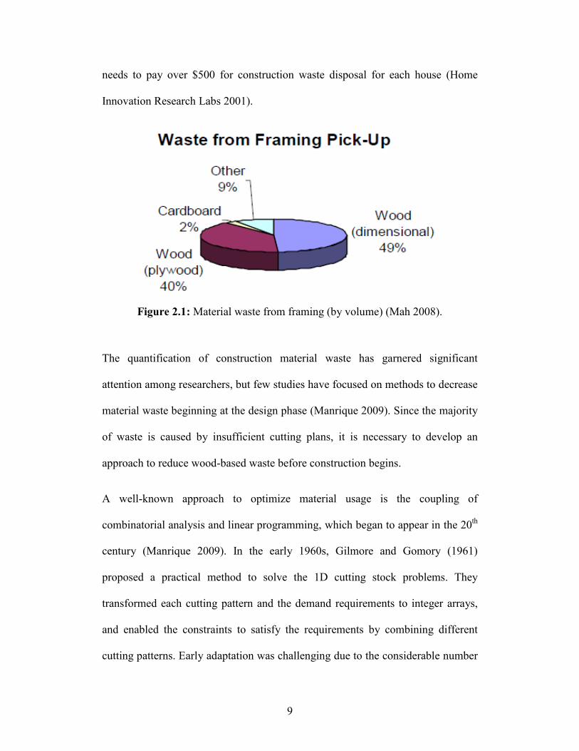
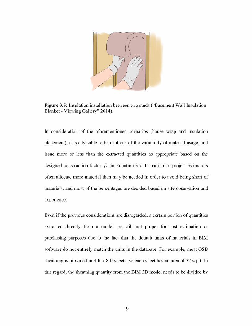
Conversely, insulation strips are only placed in the spaces between studs rather
than on top of the studs (Figure 3.5), so the extracted area (𝐴𝑖) must be larger than
the actual need (𝐴𝐼).
𝐴𝑖 = 𝐿𝑤 × 𝐻𝑤 − ∑ 𝐴𝑤𝑖𝑛𝑖=0 − ∑ 𝐴𝑑𝑖
𝑚𝑖=0 (3.4)
𝐴𝐼 = 𝐴𝑖 − 𝐴𝑓 (3.5)
𝐴𝑖: 𝐸𝑥𝑡𝑟𝑎𝑐𝑡𝑒𝑑 𝐼𝑛𝑠𝑢𝑙𝑎𝑡𝑖𝑜𝑛 𝐴𝑟𝑒𝑎
𝐿𝑤:𝑊𝑎𝑙𝑙 𝐿𝑒𝑛𝑔𝑡ℎ
𝐻𝑤:𝑊𝑎𝑙𝑙 𝐻𝑒𝑖𝑔ℎ𝑡
𝐴𝑤𝑖: 𝐴𝑟𝑒𝑎 𝑜𝑓 𝑖𝑡ℎ 𝑤𝑖𝑛𝑑𝑜𝑤 𝑜𝑝𝑒𝑛𝑖𝑛𝑔
𝐴𝑑𝑖: 𝐴𝑟𝑒𝑎 𝑜𝑓 𝑖𝑡ℎ 𝑑𝑜𝑜𝑟 𝑜𝑝𝑒𝑛𝑖𝑛𝑔
𝐴𝐼: 𝐷𝑒𝑚𝑎𝑛𝑑𝑒𝑑 𝐼𝑛𝑠𝑢𝑙𝑎𝑡𝑖𝑜𝑛 𝐴𝑟𝑒𝑎
𝐴𝑓:𝑊𝑎𝑙𝑙 𝐹𝑟𝑎𝑚𝑖𝑛𝑔 𝐴𝑟𝑒𝑎 𝑖𝑛 𝑡ℎ𝑒 𝑓𝑟𝑜𝑛𝑡 𝑣𝑖𝑒𝑤
19
Figure 3.5: Insulation installation between two studs (“Basement Wall Insulation
Blanket - Viewing Gallery” 2014).
In consideration of the aforementioned scenarios (house wrap and insulation
placement), it is advisable to be cautious of the variability of material usage, and
issue more or less than the extracted quantities as appropriate based on the
designed construction factor, 𝑓𝑐, in Equation 3.7. In particular, project estimators
often allocate more material than may be needed in order to avoid being short of
materials, and most of the percentages are decided based on site observation and
experience.
Even if the previous considerations are disregarded, a certain portion of quantities
extracted directly from a model are still not proper for cost estimation or
purchasing purposes due to the fact that the default units of materials in BIM
software do not entirely match the units in the database. For example, most OSB
sheathing is provided in 4 ft x 8 ft sheets, so each sheet has an area of 32 sq ft. In
this regard, the sheathing quantity from the BIM 3D model needs to be divided by

20
32 to convert the unit from square feet to piece. The unit converting process can
be achieved by using the unit conversion factor 𝑓𝑢 in Equation 3.7.
The situations mentioned above are common in reality, so to procure an
applicable quantity, an auxiliary property of material, called Raw Quantity (𝑄𝑅),
is added to the database. This property is designated to temporarily hold the
extracted quantities without any extra processes, and the converted quantity is
transferred to the property of Quantity (𝑄) by adding equations into the database
(Figure 3.6).
𝑄 = 𝑓(𝑄𝑅) (3.6)
𝑄 = 𝑄𝑅 ∗ 𝑓𝑢 ∗ (1 + 𝑓𝑤) ∗ (1 + 𝑓𝑐) (3.7)
𝑄:𝑄𝑢𝑎𝑛𝑡𝑖𝑡𝑦
𝑄𝑅: 𝑅𝑎𝑤 𝑄𝑢𝑎𝑛𝑡𝑖𝑡𝑦 𝑊𝑖𝑡ℎ𝑜𝑢𝑡 𝑃𝑟𝑜𝑐𝑒𝑠𝑠𝑒𝑠
𝑓𝑤:𝑀𝑎𝑡𝑒𝑟𝑖𝑎𝑙 𝑊𝑎𝑠𝑡𝑒 𝐹𝑎𝑐𝑡𝑜𝑟
𝑓𝑐: 𝐶𝑜𝑛𝑠𝑡𝑟𝑢𝑐𝑡𝑖𝑜𝑛 𝐹𝑎𝑐𝑡𝑜𝑟
𝑓𝑢: 𝑈𝑛𝑖𝑡 𝐶𝑜𝑛𝑣𝑒𝑟𝑠𝑖𝑜𝑛 𝐹𝑎𝑐𝑡𝑜𝑟

21
Figure 3.6: Database property structure.
3.1.3 Quantity Extraction
Once the BIM 3D model and database template are preloaded with the required
information, the material quantities are ready to be extracted according to
different categories (C1, C2, and C3).
All the materials in the BIM 3D model are collected, and the materials with the
identical Part Number and Module Number are accumulated to generate the
quantity, which is in turn imported to the database and assigned to the property of
Raw Quantity.
For Category 1, the quantity is the sum of the material counts.
For Category 2, the material lengths (𝑙(𝑝𝑖 & 𝑚𝐽)) are extracted and accumulated in
order to obtain the quantity.
𝐿(𝑝𝑖 & 𝑚𝐽) = ∑ 𝑙(𝑝𝑖 & 𝑚𝐽)0≤ 𝑖< 𝑚0≤𝑗<𝑛
(3.8)
For Category 3, the material areas (𝑎(𝑝𝑖 & 𝑚𝐽)) are extracted and accumulated in
order to obtain the quantity.
𝐴(𝑝𝑖 & 𝑚𝐽) = ∑ 𝑎(𝑝𝑖 & 𝑚𝐽)0≤ 𝑖< 𝑚0≤𝑗<𝑛
(3.9)
𝑝𝑖: 𝑡ℎ𝑒 𝑝𝑎𝑟𝑡 𝑛𝑢𝑚𝑏𝑒𝑟 𝑜𝑓 𝑎 𝑚𝑎𝑡𝑒𝑟𝑖𝑎𝑙
𝑚𝑗: 𝑡ℎ𝑒 𝑚𝑜𝑑𝑢𝑙𝑒 𝑛𝑢𝑚𝑏𝑒𝑟 𝑜𝑓 𝑎 𝑚𝑎𝑡𝑒𝑟𝑖𝑎𝑙 𝑏𝑒𝑙𝑜𝑛𝑔𝑠 𝑡𝑜
𝑚: 𝑡ℎ𝑒 𝑞𝑢𝑎𝑛𝑡𝑖𝑡𝑦 𝑜𝑓 𝑑𝑖𝑓𝑓𝑒𝑟𝑒𝑛𝑡 𝑡𝑦𝑝𝑒𝑠 𝑜𝑓 𝑚𝑎𝑡𝑒𝑟𝑖𝑎𝑙𝑠 𝑖𝑛 𝑡ℎ𝑒 𝐵𝐼𝑀 3𝐷 𝑚𝑜𝑑𝑒𝑙

22
𝑛: 𝑡ℎ𝑒 𝑞𝑢𝑎𝑛𝑡𝑖𝑡𝑦 𝑜𝑓 𝑚𝑜𝑑𝑢𝑙𝑒𝑠 𝑖𝑛 𝑡ℎ𝑒 𝐵𝐼𝑀 3𝐷 𝑚𝑜𝑑𝑒𝑙
As the quantities are assigned to the property of Raw Quantity, the front-loaded
formulas simultaneously calculate and transfer the processed values to Quantity,
which is regarded as the final output of quantity takeoff.
3.2 Material Optimization
This section summarizes the proposed methodology to optimize both 1D (lumber)
and 2D (sheathing) materials.
3.2.1 Lumber Optimization
Lumber is one of the most highly demanded materials in wood-based residential
construction. Poor planning of lumber cutting is common in the industry, and
results in a redundant cutting process that decreases project efficiency, generates
unnecessary waste, and reduces profit. Therefore, this research proposes to
optimize the utilization of lumber in the BIM software environment. As Figure
3.8 illustrates, the main objective of the methodology is a BIM 3D model with the
walls framed by lumber. Two algorithms, greedy and Simplex, are applied to the
model to optimize the lumber utilization with the same inputs and criteria. To
clarify the optimization methodology, four terms are mentioned frequently in the
following content, thus they need to be defined in advance.
• Dimensional Lumber: Lumber cut to standardized width and depth
dimensions (see Figure 3.7(a)).

23
• Regular Length (LR): Commercially available length of “Dimensional
Lumber” (see Figure 3.7(a))
• Lumber Piece: The lumber existing in the structure of wall framings in the
model, which is cut from dimensional lumber (3.7(b)).
• Piece Length (li): The length of “Lumber Piece”.
Figure 3.7: Examples of dimensional lumber, regular length, and lumber pieces
(Pekin Hardwood 2015; Build Your Own House 2011).
For the greedy algorithm, the lumber pieces in the model are collected and ranked
by piece length (𝑙𝑖), and only one type of dimensional lumber can be applied for
optimization, so only one lumber length (𝐿𝑅) is provided for the cutting task. The
rule for the greedy algorithm is to preferentially cut the longest lumber pieces
from the regular lumber. With respect to the Simplex algorithm, the collected
lumber pieces are grouped and ranked by piece length (𝑙𝑖), and more than one
lengths (𝐿𝑅) can be combined for the cutting task. The exhausted cutting patterns,
unit costs of regular lumber, and extracted lumber pieces constitute a relationship
of matrix representation, which is solved by the Simplex algorithm to generate a
cutting plan with minimized material cost.

24
Figure 3.8: Overview of methodology of lumber optimization.
3.2.1.1 Greedy Algorithm
The greedy algorithm is a straightforward approach to optimize the cutting of
studs. As the optimization starts, all the lumber pieces in the BIM model with
identical base dimensions (e.g., 2x3, 2x4) are collected and placed in a virtual
Lumber Pool (e.g., 2x3 pool, 2x4 pool). In each pool, lumber pieces are ranked by
length in descending order (Figure 3.9). Only one regular length (𝐿𝑅) can be used
for cutting.
25
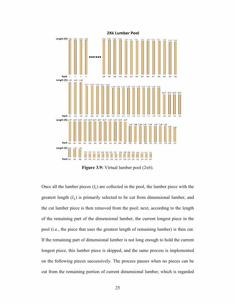
Figure 3.9: Virtual lumber pool (2x6).
Once all the lumber pieces (𝑙𝑖) are collected in the pool, the lumber piece with the
greatest length (𝑙1) is primarily selected to be cut from dimensional lumber, and
the cut lumber piece is then removed from the pool; next, according to the length
of the remaining part of the dimensional lumber, the current longest piece in the
pool (i.e., the piece that uses the greatest length of remaining lumber) is then cut.
If the remaining part of dimensional lumber is not long enough to hold the current
longest piece, this lumber piece is skipped, and the same process is implemented
on the following pieces successively. The process pauses when no pieces can be
cut from the remaining portion of current dimensional lumber, which is regarded

26
as waste. Thereafter, the lumber pieces left in the pool resume being cut from the
next dimensional lumber, until the lumber pieces in the pool are exhausted. The
flowchart of the lumber cutting process is pictured in Figure 3.10.
Collect, rank, and store lumber pieces
in a virtual pool
Cut the first lumber piece from a new
regular lumber
The current regular lumber
length >
any lumber length in the
pool?
Any lumber pieces left in the
pool?
Cut the first piece that shorter than
the current regular lumber length
Report total regular lumber usage
END
START
Figure 3.10: Flowchart of lumber cutting process.
The advantages of the greedy algorithm are that (1) independent from external
optimizing software; and (2) the processing duration is negligible. The
disadvantage, however, is the limited application: only one regular length can be
input to optimize each base dimension of lumber. As a result, most generated
cutting plans are not ultimately optimized.
Yes
Yes
No
No
27
3.2.1.2 Simplex Algorithm
Due to the limitation of the greedy algorithm, a more intelligent method is
developed based on Simplex algorithm. The benefit of Simplex algorithm is the
feasibility of combining multiple regular lengths, which improves the capability
of producing an optimized cutting plan. While obtaining multiple regular lengths,
the corresponding unit value or cost (vi) is obligatory to be assigned to each piece
of regular lumber, such that the objective is minimizing the sum of each product
of lumber quantity and its unit value or cost. After obtaining the regular lengths
and the respective values, the stock-cutting problem can be transformed to Linear
Programming Optimization with matrix representation, which contains an
objective function, coefficient matrix, constraints, target array, and decision
variables.
The lumber pieces are collected and categorized in the same manner as the greedy
algorithm, but where Simplex differs is that the lumber pieces in each lumber pool
require further processing. This is achieved by grouping the lumber pieces by
length and then ranking the groups in a descending order. The quantity of each
lumber piece length is regarded as one element in a Target Array (𝐴𝑇), which is a
one-dimensional array containing N elements, and N herein represents the
quantity of groups.
𝐴𝑇 = [𝑞1, 𝑞2, 𝑞3 ……𝑞𝑁−1, 𝑞𝑁]
𝑞𝑖: the quantity of the ith
length of lumber piece is demanded in the project
𝑁: the number of tree structure levels or the lumber piece groups

28
Using the quantities derived from the grouped lumber pool in Figure 3.11, an
example Target Array (𝐴𝑇) is [151, 8, 2, 3, 5, 10, 16, 8, 1, 1, 3, 16].
Figure 3.11: Grouped lumber pool (2x6).
Using the established quantities, all the possible cutting patterns need to be
enumerated onto each regular length of lumber provided, and different cutting
patterns are combined to ensure the quantities of cut pieces equalize or are beyond
the corresponding demand of the collected lumber pieces (Target Array). In order
to exhaust all the cutting patterns, the tree structure method is implemented
(Figure 3.12).
The tree structure has multiple levels of node and branch, and each level holds
one lumber piece length (li); longer pieces are found higher on the structure level
and shorter pieces, proportionately, are found lower on the structure level.
Therefore, the number of levels (N) should be equal to the number of lumber
groups or the elements in a Target Array. Each tree starts from a top node, which
represents a regular length (LR). Each branch represents the quantity of instances
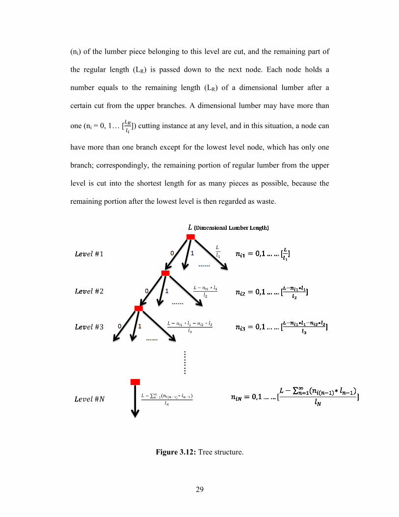
29
(ni) of the lumber piece belonging to this level are cut, and the remaining part of
the regular length (LR) is passed down to the next node. Each node holds a
number equals to the remaining length (LR) of a dimensional lumber after a
certain cut from the upper branches. A dimensional lumber may have more than
one (ni = 0, 1… [𝐿𝑅
𝑙𝑖]) cutting instance at any level, and in this situation, a node can
have more than one branch except for the lowest level node, which has only one
branch; correspondingly, the remaining portion of regular lumber from the upper
level is cut into the shortest length for as many pieces as possible, because the
remaining portion after the lowest level is then regarded as waste.
Figure 3.12: Tree structure.

30
The quantities of instances from each branch are gathered to form one cutting
pattern, which is represented as an integer array (𝐴𝑖)
𝐴𝑖 = [𝑛𝑖1, 𝑛𝑖2, 𝑛𝑖3 ……𝑛𝑖(𝑁−1), 𝑛𝑖𝑁]
M: quantity of total cutting pattern
𝐴𝑖: the ith
cutting pattern from tree structure, i = 1, 2, 3……M
𝑛𝑖𝑗: the quantity of jth
lumber piece is cut in ith
cutting pattern, j = 1, 2, 3…N, i =
1, 2, 3……M
The collection of all the arrays becomes an M by N matrix, M represents the
quantity of total cutting patterns, and N represents the quantity of different lumber
piece lengths.
𝐴𝑟𝑟𝑎𝑦1 = [𝑛11, 𝑛12, 𝑛13, 𝑛14 ……𝑛1(𝑁−3), 𝑛1(𝑁−2), 𝑛1(𝑁−1), 𝑛1𝑁]
𝐴𝑟𝑟𝑎𝑦2 = [𝑛21, 𝑛22, 𝑛23, 𝑛24 ……𝑛2(𝑁−3), 𝑛2(𝑁−2), 𝑛2(𝑁−1), 𝑛2𝑁]
𝐴𝑟𝑟𝑎𝑦𝑀 = [𝑛𝑀1, 𝑛𝑀2, 𝑛𝑀3, 𝑛𝑀4 ……𝑛𝑀(𝑁−3), 𝑛𝑀(𝑁−2), 𝑛𝑀(𝑁−1), 𝑛𝑀𝑁]

31
[
𝑛11 𝑛12 𝑛13
𝑛21 𝑛22 𝑛23
𝑛31 𝑛32 𝑛33
⋯
𝑛1(𝑁−2) 𝑛1(𝑁−1) 𝑛1𝑁
𝑛2(𝑁−2) 𝑛2(𝑁−1) 𝑛2𝑁
𝑛3(𝑁−2) 𝑛3(𝑁−1) 𝑛3𝑁
⋮ ⋱ ⋮𝑛(𝑀−2)1 𝑛(𝑀−2)2 𝑛(𝑀−2)3
𝑛(𝑀−1)1 𝑛(𝑀−1)2 𝑛(𝑀−1)3
𝑛𝑀1 𝑛𝑀2 𝑛𝑀3
⋯
𝑛(𝑀−2)(𝑁−2) 𝑛(𝑀−2)(𝑁−1) 𝑛(𝑀−2)𝑁
𝑛(𝑀−1)(𝑁−2) 𝑛(𝑀−1)(𝑁−1) 𝑛(𝑀−1)𝑀
𝑛𝑀(𝑁−2) 𝑛𝑀(𝑁−1) 𝑛𝑀𝑁 ]
To implement the Simplex method, the M by N matrix needs to be transposed to
an N by M matrix; in other words, these integer arrays are placed vertically, and
the new matrix is called Coefficient Matrix. A decision variable is also required to
solve the whole problem, and it should be represented by an array with M
elements. Each element in this array means the quantity of dimensional lumber
used to be cut in the corresponding manner.
𝐴𝑑 = [𝑥1, 𝑥2, 𝑥3 ……𝑥𝑀−1, 𝑥𝑀]
𝐴𝑑: Decision Variable Array
In the meantime, a Coefficient Array is also formed by the lumber unit value or
cost (vi).
𝐴𝑐 = [𝑣1, 𝑣2, 𝑣3 ……𝑣𝑀−1, 𝑣𝑀]
𝐴𝑐: Coefficient Array
The relation between the Coefficient Matrix, Decision Variable Array and Target
Array is shown below.
𝐶𝑜𝑒𝑓𝑓𝑖𝑐𝑖𝑒𝑛𝑡 𝑀𝑎𝑡𝑟𝑖𝑥 × 𝐷𝑒𝑐𝑖𝑠𝑖𝑜𝑛 𝑉𝑎𝑟𝑖𝑎𝑏𝑙𝑒 𝐴𝑟𝑟𝑎𝑦 ≥ 𝑇𝑎𝑟𝑔𝑒𝑡 𝐴𝑟𝑟𝑎𝑦

32
[ 𝑛11 𝑛12 𝑛13
𝑛21 𝑛22 𝑛23𝑛31 𝑛32 𝑛33
⋯𝑛1(𝑁−2) 𝑛1(𝑁−1) 𝑛1𝑁𝑛2(𝑁−2) 𝑛2(𝑁−1) 𝑛2𝑁𝑛3(𝑁−2) 𝑛3(𝑁−1) 𝑛3𝑁
⋮ ⋱ ⋮𝑛(𝑀−2)1 𝑛(𝑀−2)2 𝑛(𝑀−2)3𝑛(𝑀−1)1 𝑛(𝑀−1)2 𝑛(𝑀−1)3𝑛𝑀1 𝑛𝑀2 𝑛𝑀3
⋯
𝑛(𝑀−2)(𝑁−2) 𝑛(𝑀−2)(𝑁−1) 𝑛(𝑀−2)𝑁𝑛(𝑀−1)(𝑁−2) 𝑛(𝑀−1)(𝑁−1) 𝑛(𝑀−1)𝑀𝑛𝑀(𝑁−2) 𝑛𝑀(𝑁−1) 𝑛𝑀𝑁 ]
𝑇
×
[
𝑥1𝑥2𝑥3
⋮𝑥𝑀−2
𝑥𝑀−1𝑥𝑀 ]
≥
[
𝑞1𝑞2𝑞3
⋮𝑞𝑁−2
𝑞𝑁−1𝑞𝑁 ]
(3.10)
The final goal is to provide an optimized cutting scenario to minimize the total
material cost, which is represented by the objective function.
𝑀𝑖𝑛𝑖𝑚𝑖𝑧𝑖𝑛𝑔: 𝑥1 ∗ 𝑣1 + 𝑥2 ∗ 𝑣2 + 𝑥3 ∗ 𝑣3 + ⋯+ 𝑥𝑀−1 ∗ 𝑣𝑀−1 + 𝑥𝑀 ∗ 𝑣𝑀
Some piece lengths are longer than the longest dimensional lumber, for example,
top and bottom plates are always as long as the modular, which could easily be 72
ft in length. In this optimization, these oversized lumbers are not considered.
Based on research’s knowledge, different companies have different approaches to
obtain these lumbers, and many choose to purchase finger joint lumber or special
lumber directly from the supplier without any specific processing in the factory.
3.2.1.3 Algorithm Comparison
The lumber optimization problem can be solved by both of the algorithms, Greedy
and Simplex. Greedy will be the primary algorithm to be applied in the industry,
since the theory is easily to be implemented by codes compilation and the
processing time is negligible. The limitation of Greedy is that only one type of
regular lumber is allowed to be applied for cutting process and the most of results
are not fully optimized. However, Simplex algorithm can overcome the limitation
by integrating multiple types of regular lumbers, and it is capable to provide an
exactly optimized solution. Hence it is suitable for scientific purpose. The

33
disadvantage of Simplex is the need of external optimizer, and the processing time
becomes unacceptable for large data set (Table 3.1).
Table 3.1 Greedy and Simplex algorithms comparison
Advantage Disadvantage
Greedy 1. Easy to compile
2. Negligible processing time
1. Result is not fully optimized
2. Only one type of regular lumber
can be considered for cutting
Simplex 1. Fully optimized result
2. Feasible to integrate multiple
types of regular lumbers
1. Need of external library
2. Long processing time for large
data set
3.2.2 Sheathing Optimization
In wood frame residential construction, sheathing is utilized almost as widely as is
lumber. Furthermore, the sheathing cutting process (2D) is more complicated and
prone to waste than is lumber cutting (1D). Hence, this research proposes a
methodology to facilitate the sheathing cutting process in order to enhance
sheathing usage by integrating the BIM software with an optimization algorithm.
In this research, the methodology is developed in the environment of Autodesk
Revit, which is a widely utilized BIM software for architectural and structural
drawing.
However, efforts to optimize sheathing usage face two main obstacles: (1) the
Revit 3D model does not have a visible component to represent sheathing, such
that the sheathing information is only accessible by further investigating the host
34
element (e.g., wall, floor, and roof) of sheathing; and (2) Revit is configured to
regard sheathing and other area materials (such as gypsum board) as whole pieces,
where the area of material is equal to the closed area of the host object. This
configuration is unable to account for actual construction. Furthermore, the model
does not show the seams between two adjacent sheathing pieces, i.e., the
sheathing layout on the wall framing.
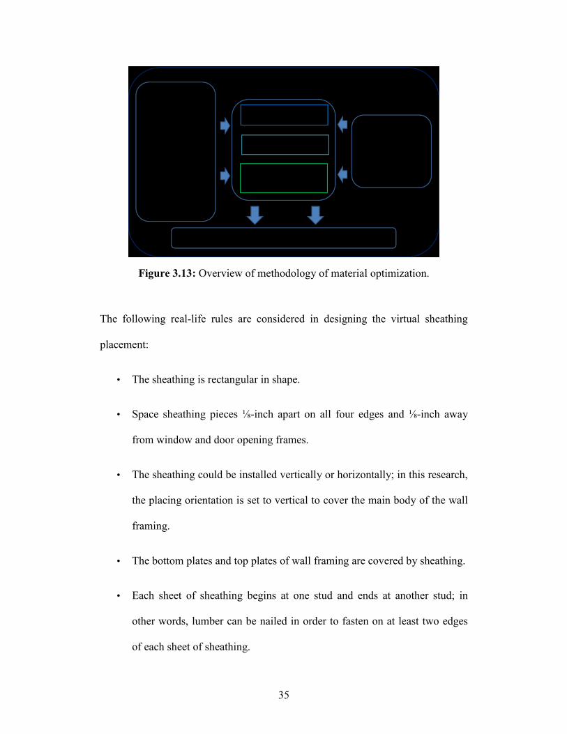
As Figure 3.13 illustrates, the sheathing pieces are visualized and installed on the
wall framing in the model based on the wall configuration and stud locations, and
the installed sheathing pieces are collected, reoriented, and ranked. Moreover, the
organized sheathing pieces are cut from a certain dimension of regular sheathing
by following the greedy and bottom-left heuristic algorithms. As a result, the
realistic sheathing usage and optimized cutting plan are exported. A precondition
for placing and visualizing sheathing, which is also a requirement for lumber
optimization, is that the framing of the walls must be completed in the model prior
to carrying out the material optimization. Based on the wall framing, sheathing
placement can be achieved.
35
Figure 3.13: Overview of methodology of material optimization.
The following real-life rules are considered in designing the virtual sheathing
placement:
• The sheathing is rectangular in shape.
• Space sheathing pieces ⅛-inch apart on all four edges and ⅛-inch away
from window and door opening frames.
• The sheathing could be installed vertically or horizontally; in this research,
the placing orientation is set to vertical to cover the main body of the wall
framing.
• The bottom plates and top plates of wall framing are covered by sheathing.
• Each sheet of sheathing begins at one stud and ends at another stud; in
other words, lumber can be nailed in order to fasten on at least two edges
of each sheet of sheathing.

36
To visualize the sheets of sheathing in the model, a new Revit family of sheathing
is created (Figure 3.14). The sheathing family has five important parameters:
• Height: height of sheathing.
• Length: length of sheathing.
• Label: the label located at the center of sheathing, and is visible from both
sides.
• Locator: the point on the bottom-inside corner of the sheathing nearer to
the framing point, which can be assigned three-dimensional coordinates in
order to locate the sheathing on the wall framing.
• Host: the wall onto which sheathing is installed.
Figure 3.14: Revit family—sheathing.
37
So far, two sheathing terms are referred to in this research, and both terms need to
be specified to avoid ambiguity:
• Regular Sheathing (length: LR, height: HR) represents the stocked
sheathing with nominal dimensions, and they have not been cut.
• Sheathing Piece (length: li, height: hi) means sheathing framed on the
wall. The created Revit sheathing family framed on the wall in the model
is the Sheathing Piece.
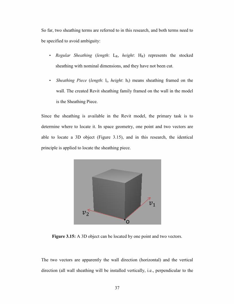
Since the sheathing is available in the Revit model, the primary task is to
determine where to locate it. In space geometry, one point and two vectors are
able to locate a 3D object (Figure 3.15), and in this research, the identical
principle is applied to locate the sheathing piece.
Figure 3.15: A 3D object can be located by one point and two vectors.
The two vectors are apparently the wall direction (horizontal) and the vertical
direction (all wall sheathing will be installed vertically, i.e., perpendicular to the
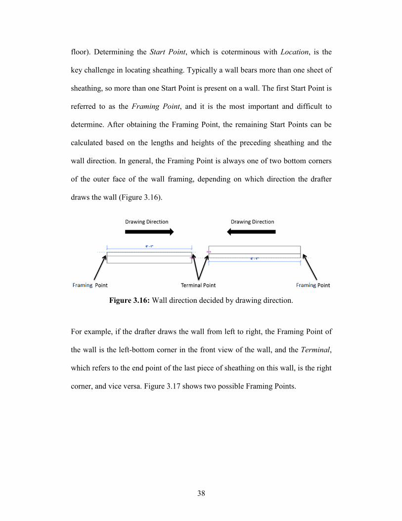
38
floor). Determining the Start Point, which is coterminous with Location, is the
key challenge in locating sheathing. Typically a wall bears more than one sheet of
sheathing, so more than one Start Point is present on a wall. The first Start Point is
referred to as the Framing Point, and it is the most important and difficult to
determine. After obtaining the Framing Point, the remaining Start Points can be
calculated based on the lengths and heights of the preceding sheathing and the
wall direction. In general, the Framing Point is always one of two bottom corners
of the outer face of the wall framing, depending on which direction the drafter
draws the wall (Figure 3.16).
Figure 3.16: Wall direction decided by drawing direction.
For example, if the drafter draws the wall from left to right, the Framing Point of
the wall is the left-bottom corner in the front view of the wall, and the Terminal,
which refers to the end point of the last piece of sheathing on this wall, is the right
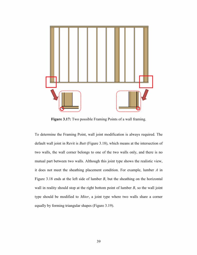
corner, and vice versa. Figure 3.17 shows two possible Framing Points.
39
Figure 3.17: Two possible Framing Points of a wall framing.
To determine the Framing Point, wall joint modification is always required. The
default wall joint in Revit is Butt (Figure 3.18), which means at the intersection of
two walls, the wall corner belongs to one of the two walls only, and there is no
mutual part between two walls. Although this joint type shows the realistic view,
it does not meet the sheathing placement condition. For example, lumber A in
Figure 3.18 ends at the left side of lumber B, but the sheathing on the horizontal
wall in reality should stop at the right bottom point of lumber B, so the wall joint
type should be modified to Miter, a joint type where two walls share a corner
equally by forming triangular shapes (Figure 3.19).

40
Figure 3.18: Butt wall joint type.
Figure 3.19: Modify Butt wall joint to Miter.

41
Even at this step, it is still not practical to obtain the Framing Point directly with
Revit functions. However, further investigation shows that the Framing Points of
wall and wall framing are perfectly matching after overlapping them (Figure 3.20
and Figure 3.21), and this feature leads to the optimal approach to determine the
Framing Point.
Figure 3.20: The overlap of wall and wall framing; Framing Points are identical
and circled in red.

42
Figure 3.21: Top view of the overlap of wall and wall framing; Framing Point is
circled in red.
Some pertinent wall layer relationships are also discovered, and point coordinates
(Figure 3.22) and wall layer thicknesses (Figure 3.23) are accessible from Revit.
All are essential to derive the three dimensional coordinate of the Framing Point.
Based on the gathered information, the Framing Point can be calculated by means
of analytically.
• Mid Point (Mx, My, Mz): Centre point of the bottom intersection line of two
walls (accessible from Revit).
• Exterior Point (Ex, Ey, Ez): Bottom corner point of exterior face of a wall
(accessible from Revit).

43
• Interior Point (Ix, Iy, Iz): Bottom corner point of interior face of a wall
(accessible from Revit).
• Total Layer (Tt): Total layer thickness (accessible from Revit).
• Interior Layer (Ti): Interior layer thickness (Structure layer + Inner side
layers of structure layer) (accessible from Revit).
Figure 3.22: Highlight of wall bottom corner.
Figure 3.23: Wall layers with thicknesses.
Since the placement of sheathing always starts from the floor level, which means
the Z-axis of all the Framing Points is 0, only the X-axis and Y-axis need to be
calculated to locate the Framing Point. The required values can be obtained by

44
implementing Revit API functions, and Triangle Proportionality is utilized to
calculate the coordinates of the Framing Point (Fx, Fy, Fz).
𝐹𝑥 = 𝐼𝑥 +2×(𝑀𝑥−𝐼𝑥)
𝑇𝑡× 𝑇𝑖 (3.11)
𝐹𝑦 = 𝐼𝑦 +2×(𝑀𝑦−𝐼𝑦)
𝑇𝑡× 𝑇𝑖 (3.12)
𝐹𝑧 = 𝐼𝑧 = 𝑀𝑧 = 0 (3.13)
After obtaining the Framing Point, the succeeding Start Points can be calculated
based on this Framing Point and sheathing height, length, and wall direction. In
addition, it is imperative to understand the basic components and dimensions of a
typical wall framing (Figure. 3.24) in order to further investigate the sheathing
placement.
Figure 3.24: Components and dimensions of wall framing.
𝐻𝑤:𝑊𝑎𝑙𝑙 𝐹𝑟𝑎𝑚𝑖𝑛𝑔 𝐻𝑒𝑖𝑔ℎ𝑡

45
𝐿𝑤:𝑊𝑎𝑙𝑙 𝐹𝑟𝑎𝑚𝑖𝑛𝑔 𝐿𝑒𝑛𝑔𝑡ℎ
𝑊𝑑𝑖:𝑊𝑖𝑑𝑡ℎ 𝑜𝑓 𝑖𝑡ℎ 𝐷𝑜𝑜𝑟 𝐹𝑟𝑎𝑚𝑖𝑛𝑔
𝑊𝑤𝑖:𝑊𝑖𝑑𝑡ℎ 𝑜𝑓 𝑖𝑡ℎ 𝑊𝑖𝑛𝑑𝑜𝑤 𝐹𝑟𝑎𝑚𝑖𝑛𝑔
𝐻𝑑𝑗𝑖: 𝐽𝑎𝑐𝑘 𝑆𝑡𝑢𝑑 𝐻𝑒𝑖𝑔ℎ𝑡 𝑜𝑓 𝑖𝑡ℎ 𝐷𝑜𝑜𝑟 𝐹𝑟𝑎𝑚𝑖𝑛𝑔
𝐻𝑑𝑘𝑖: 𝐾𝑖𝑛𝑔 𝑆𝑡𝑢𝑑 𝐻𝑒𝑖𝑔ℎ𝑡 𝑜𝑓 𝑖𝑡ℎ 𝐷𝑜𝑜𝑟 𝐹𝑟𝑎𝑚𝑖𝑛𝑔
𝐻𝑤𝑗𝑖: 𝐽𝑎𝑐𝑘 𝑆𝑡𝑢𝑑 𝐻𝑒𝑖𝑔ℎ𝑡 𝑜𝑓 𝑖𝑡ℎ 𝑊𝑖𝑛𝑑𝑜𝑤 𝐹𝑟𝑎𝑚𝑖𝑛𝑔
𝐻𝑘𝑤𝑖: 𝐾𝑖𝑛𝑔 𝑆𝑡𝑢𝑑 𝐻𝑒𝑖𝑔ℎ𝑡 𝑜𝑓 𝑖𝑡ℎ 𝑊𝑖𝑛𝑑𝑜𝑤 𝐹𝑟𝑎𝑚𝑖𝑛𝑔
𝐻𝑤𝑐𝑖: 𝐶𝑟𝑖𝑝𝑝𝑙𝑒 𝐻𝑒𝑖𝑔ℎ𝑡 𝑜𝑓 𝑖𝑡ℎ 𝑊𝑖𝑛𝑑𝑜𝑤 𝐹𝑟𝑎𝑚𝑖𝑛𝑔
𝐻𝑑𝑐𝑖: 𝐶𝑟𝑖𝑝𝑝𝑙𝑒 𝐻𝑒𝑖𝑔ℎ𝑡 𝑜𝑓 𝑖𝑡ℎ 𝐷𝑜𝑜𝑟 𝐹𝑟𝑎𝑚𝑖𝑛𝑔
𝑇𝑑𝑠𝑝𝑖: 𝐷𝑜𝑢𝑏𝑙𝑒 𝑆𝑖𝑙𝑙 𝑃𝑙𝑎𝑡𝑒𝑠 𝑇ℎ𝑖𝑐𝑘𝑛𝑒𝑠𝑠 𝑜𝑓 𝑖𝑡ℎ 𝑊𝑖𝑛𝑑𝑜𝑤 𝐹𝑟𝑎𝑚𝑖𝑛𝑔
𝑇𝑠𝑏𝑝: 𝑆𝑖𝑛𝑔𝑙𝑒 𝐵𝑜𝑡𝑡𝑜𝑚 𝑃𝑙𝑎𝑡𝑒 𝑇ℎ𝑖𝑐𝑘𝑛𝑒𝑠𝑠 𝑜𝑓 𝑊𝑎𝑙𝑙 𝐹𝑟𝑎𝑚𝑖𝑛𝑔
𝑍: 𝐵𝑜𝑡𝑡𝑜𝑚 𝐹𝑎𝑐𝑒 𝐿𝑒𝑣𝑒𝑙 𝑜𝑓 𝑆𝑖𝑛𝑔𝑙𝑒 𝐵𝑜𝑡𝑡𝑜𝑚 𝑃𝑙𝑎𝑡𝑒 ("0" 𝑓𝑜𝑟 𝑎𝑙𝑙 𝑠𝑖𝑛𝑔𝑙𝑒 𝑠𝑡𝑜𝑟𝑒𝑦 𝑚𝑜𝑑𝑢𝑙𝑒𝑠)
To place the sheathing on the wall framing, the window and door framing
components are differentiated from the regular wall framing. For the window and
door framing, the height of sheathings is set to strictly cover the door’s upper
framing and window’s upper and lower framings (Figure 3.25); the corresponding
heights are shown below.
Sheathing height above the ith door: ℎ𝑖 = 𝐻𝑤 − 𝑇𝑠𝑏𝑝 − 𝐻𝑑𝑗𝑖 (3.14)
Sheathing height above the ith window: ℎ𝑖 = 𝐻𝑤 − 𝑇𝑠𝑏𝑝 − 𝐻𝑤𝑗𝑖 (3.15)
Sheathing height below the ith window: ℎ𝑖 = 𝐻𝑤𝑐𝑖 + 𝑇𝑠𝑏𝑝 + 𝑇𝑑𝑠𝑝𝑖 (3.16)

46
Figure 3.25: Height determination rule (window and door).
After the window and door framing parts are covered by sheathing, the rest of the
wall is regarded as the wall without windows or doors, and the height
determination rules are shown below.
• If a wall height is lower than the nominal height of regular sheathing,
which means only one sheathing can cover the whole height of the wall,
the height of the sheathing is the height of the wall (Figure 3.26).
• Sheathing height: ℎ𝑖 = 𝐻𝑤 (if 𝐻𝑅 ≥ 𝐻𝑤) (3.17)
Figure 3.26: Height determination rule (sheathing height is higher than wall
height).

47
• If a wall height is higher than the nominal height of regular sheathing, at
least two pieces of sheathing are needed to cover the whole wall height;
the lower part is the full height of regular sheathing, and the height of the
upper part is the remaining wall height (Figure 3.27).
Upper Sheathing height: ℎ𝑖 = 𝐻𝑤 − 𝐻𝑅 (if 𝐻𝑅 < 𝐻𝑤) (3.18)
Lower Sheathing height: ℎ𝑖 = 𝐻𝑅 (if 𝐻𝑅 < 𝐻𝑤) (3.19)
Figure 3.27: Height determination rule (sheathing height is lower than wall
height).
Since wall length is most often longer than wall height, the determination of
sheathing length is apparently more complicated. In this situation, the sheathing
lengths of the framing portions above a door opening and above and below a
window opening are determined primarily, which are the respective window and
door widths (see SH3, SH4, and SH5 in Figure 3.30). Subsequently, (the distance
of) two points are utilized to determine the sheathing length for the main body of
the wall framing; one point is Start Point, and the other is End Point, which is the
location at which the placed sheathing is cut, and the End Point must be at the
48
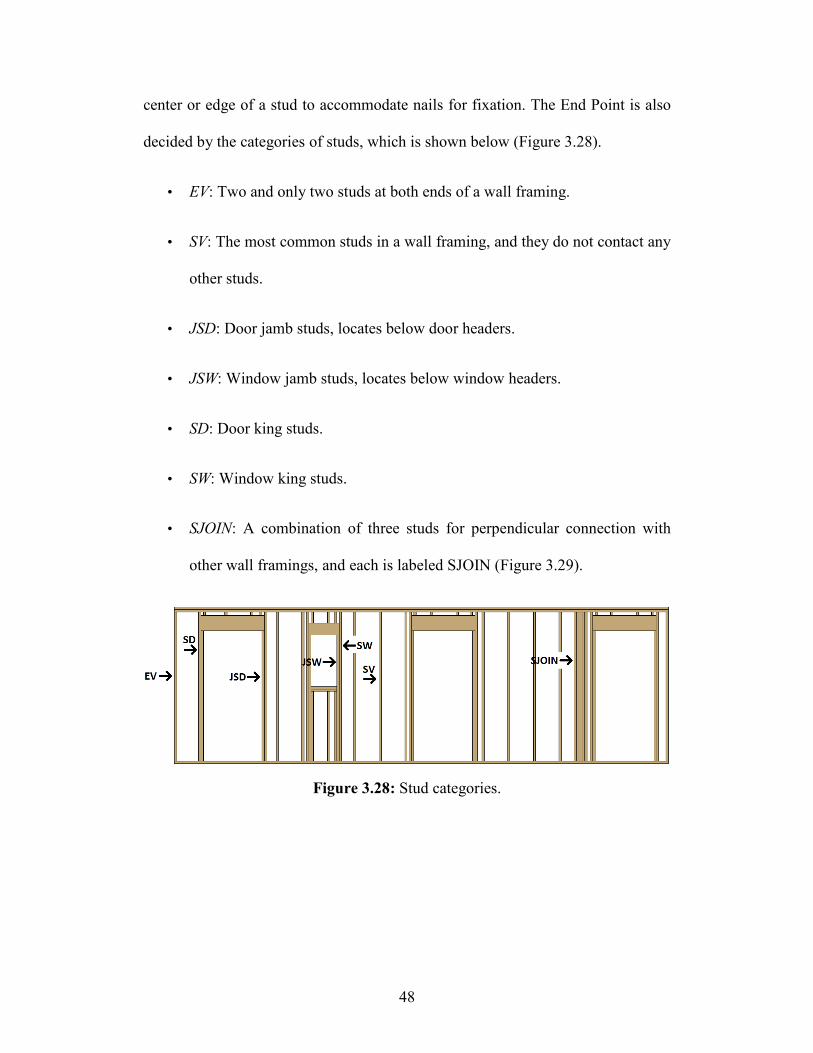
center or edge of a stud to accommodate nails for fixation. The End Point is also
decided by the categories of studs, which is shown below (Figure 3.28).
• EV: Two and only two studs at both ends of a wall framing.
• SV: The most common studs in a wall framing, and they do not contact any
other studs.
• JSD: Door jamb studs, locates below door headers.
• JSW: Window jamb studs, locates below window headers.
• SD: Door king studs.
• SW: Window king studs.
• SJOIN: A combination of three studs for perpendicular connection with
other wall framings, and each is labeled SJOIN (Figure 3.29).
Figure 3.28: Stud categories.

49
Figure 3.29: Highlight of SJOIN studs.
All the studs are divided into two groups according to the category. Group 1
incorporates the studs of EV, JSD and JSW, and the End Point of Group 1 is
located at the far bottom corner in order to cover the whole width of the stud
placed with the sheathing. Group 2 consists of SV, SD, SW and two parallel
SJOIN studs are in the second group. The End Point of Group 2 is located at the
center of the studs as the Group 2 stud is invariably shared by two pieces of
sheathing on both sides.
The first piece of sheathing starts from the Framing Point and terminates at the
next End Point of Group 1 on the occasion that the distance between two points is
shorter than the nominal length of regular sheathing. If this condition is not
satisfied, this piece of sheathing is shortened to an End Point of Group 2, which
results in various possible distances. Among all the distances, the lengths greater

50
than regular sheathing length are filtered out, and the greatest length is selected
from the refined distances to be the length of this piece of sheathing.
𝑙𝑖 = {𝐷1, 𝐷1 ≤ 𝐿𝑅
𝐷2, 𝐷1 > 𝐿𝑅 (3.20)
𝐷1: Distance between the current Start Point and the closest Group 1 End Point
following the wall direction.
𝐷2: Distance between the current Start Point and the furthest Group 2 End Point
following the wall direction, where distance always has a value less than the
regular sheathing length.
Under certain circumstances, the wall height is higher than the nominal height of
regular sheathing (see SH6, SH7 and SH8 in Figure 3.30), thus another level of
sheathing is required to cover the upper part of framing, which is usually more
narrow than the regular sheathing f nominal length; consequently, the sheathing is
placed horizontally (see SH9, SH10 in Figure 3.30).
Figure 3.30: Sheathing length determination.

51
So far, Framing Point, sheathing lengths, and sheathing heights are available, and
the information is sufficient to fulfill the placement of the first sheathing on the
wall framing. The succeeding sheathing placement always starts from a Start
Point (Px, Py, Pz), which can be generated from a previous Start Point (px, py, pz)
and the configuration of the previous sheathing, such as height (hi) and length (li),
and the host wall direction (rx, ry, rz). Different approaches are implemented to
determine new Start Points dealing with different conditions.
• If sheathing placement does not associate with doors or windows, the new
Start Point is always the sheathing bottom corner which locates farther
from the Framing Point (Figure 3.31).
𝑃𝑥 = 𝐿𝑖 ∗ 𝑟𝑥 + 𝑝𝑥 (3.21)
𝑃𝑦 = 𝐿𝑖 ∗ 𝑟𝑦 + 𝑝𝑦 (3.22)
𝑃𝑧 = 𝐿𝑖 ∗ 𝑟𝑧 + 𝑝𝑧 (3.23)
Figure 3.31: Start Point determination (wall without window or door).

52
• If sheathing is cut off along the edge of a jack stud of a door (JSD), two
new Start Points are generated. The New Start Point 1 (Px, Py, Pz) is
located below the other JSD with the same z-coordinate value (Pz = pz) in
order to continue sheathing placement on the main wall framing (Figure
3.32).
𝑃𝑥 = (𝑙𝑖 + 𝑊𝑑𝑖) ∗ 𝑟𝑥 + 𝑝𝑥 (3.24)
𝑃𝑦 = (𝑙𝑖 + 𝑊𝑑𝑖) ∗ 𝑟𝑦 + 𝑝𝑦 (3.25)
𝑃𝑧 = (𝑙𝑖 + 𝑊𝑑𝑖) ∗ 𝑟𝑧 + 𝑝𝑧 (3.26)
The New Start Point 2 (Px, Py, Pz) locates the current JSD tip point, which
is farther from the Framing Point (Figure 3.32), and this Start Point
commences the sheathing placement above the door opening.
𝑃𝑥 = 𝑙𝑖 ∗ 𝑟𝑥 + 𝑝𝑥 (3.21)
𝑃𝑦 = 𝑙𝑖 ∗ 𝑟𝑦 + 𝑝𝑦 (3.22)
𝑃𝑧 = 𝑙𝑖 ∗ 𝑟𝑧 + 𝑝𝑧 + 𝐻𝑑𝑗𝑖 (3.27)

53
Figure 3.32: Start Point determination (door).
• If sheathing is cut off along the edge of a jack stud of a window (JSW),
three new Start Points are generated. The New Start Point 1 (Px, Py, Pz) is
located to place the sheathing on the opposite side of the window opening.
𝑃𝑥 = (𝑙𝑖 + 𝑊𝑤𝑖) ∗ 𝑟𝑥 + 𝑝𝑥 (3.28)
𝑃𝑦 = (𝑙𝑖 + 𝑊𝑤𝑖) ∗ 𝑟𝑦 + 𝑝𝑦 (3.29)
𝑃𝑧 = (𝑙𝑖 + 𝑊𝑤𝑖) ∗ 𝑟𝑧 + 𝑝𝑧 (3.30)
The New Start Point 2 (Px, Py, Pz) is the tip point of a JSW, which is
farther from the Framing Point (Figure 3.33).
𝑃𝑥 = 𝑙𝑖 ∗ 𝑟𝑥 + 𝑝𝑥 (3.21)
𝑃𝑦 = 𝑙𝑖 ∗ 𝑟𝑦 + 𝑝𝑦 (3.22)
𝑃𝑧 = 𝑙𝑖 ∗ 𝑟𝑧 + 𝑝𝑧 + 𝐻𝑤𝑗𝑖 (3.31)

54
The New Start Point 3 (Px, Py, Pz) locates below the current JSD with the
same z-coordinate value (Pz = pz) in order to place the sheathing below the
window opening (Figure 3.33).
𝑃𝑥 = 𝑙𝑖 ∗ 𝑟𝑥 + 𝑝𝑥 (3.21)
𝑃𝑦 = 𝑙𝑖 ∗ 𝑟𝑦 + 𝑝𝑦 (3.22)
𝑃𝑧 = 𝑙𝑖 ∗ 𝑟𝑧 + 𝑝𝑧 (3.23)
Figure 3.33: Start Point determination (window).
• If a wall height is higher than the nominal height of regular sheathing,
another piece of sheathing is required above the current sheathing, so an
additional new Start Point (Px, Py, Pz) is developed above the current Start
Point with an elevation equal to the current piece of sheathing height
(Figure 3.34).
𝑃𝑥 = 𝑝𝑥 (3.32)

55
𝑃𝑦 = 𝑝𝑦 (3.33)
𝑃𝑧 = ℎ𝑖 + 𝑝𝑧 (3.34)
Figure 3.34: Start Point determination (wall height is higher than sheathing
height).
Following these principles, the placement of sheathing can be achieved. Each
piece of sheathing has a unique label at the centre for differentiation. Generally,
the label is combined by the host wall ID and the sheathing ID. For example, if a
piece of sheathing locates on an exterior wall “AX4” and the sheathing has an ID
of “S27”, the label should be “AX4-S27” (Figure 3.35).
Figure 3.35: Sheathing labels.
56
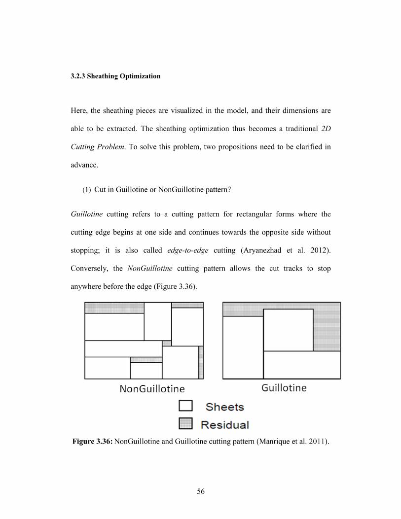
3.2.3 Sheathing Optimization
Here, the sheathing pieces are visualized in the model, and their dimensions are
able to be extracted. The sheathing optimization thus becomes a traditional 2D
Cutting Problem. To solve this problem, two propositions need to be clarified in
advance.
(1) Cut in Guillotine or NonGuillotine pattern?
Guillotine cutting refers to a cutting pattern for rectangular forms where the
cutting edge begins at one side and continues towards the opposite side without
stopping; it is also called edge-to-edge cutting (Aryanezhad et al. 2012).
Conversely, the NonGuillotine cutting pattern allows the cut tracks to stop
anywhere before the edge (Figure 3.36).
Figure 3.36: NonGuillotine and Guillotine cutting pattern (Manrique et al. 2011).

57
In terms of material saving, NonGuillotine is an optimal pattern; but if
considering the efficiency of the cutting process, Guillotine saves considerably
more time and does not require the same level of accuracy in measurements or of
skill in operators.
(2) Can sheathing be rotated or not?
If the sheathing is set to be rotatable, then it is not necessary for the four sides of a
piece of sheathing to be parallel with the edges of regular sheathing. The rotatable
cutting pattern has an increased capability of utilizing the regular sheathing
sufficiently and accomplishing certain cutting tasks, which are unachievable for
orientation-fixed patterns. For example, Figure 3.37 shows that the only way to
cut five squares (four 40 x 40 squares and one 28.28 x 28.28 square) from a large
square (100 x 100) is rotating the centre square by 45 degrees. However, this
cutting pattern has the same disadvantage as the NonGuillotine, which requires
additional labour hours, more accurate measurements, and higher skilled
operators.

58
Figure 3.37: The only way to cut five small certain squares in a large square
(Solving the 2D Packing Problem 2007).
In Canada, it is sensible to consider the labour saving rather than material saving
in view of the high local labour rate, thus the sheathing optimization is
implemented based on the Guillotine and orientation-fixed cutting pattern. The
following detailed procedure includes two rounds, which are represented by a
flowchart shown in Figure 3.38.

59
Collect sheathing pieces from 3D model, rotate pieces with longer l than h by 90°,
switch nomination of l and h. Rank pieces by h first and l second, store
in a virtual pool
Check ifh of any piece
>available L of
current regular sheathing
Orient regular sheathing vertically
Orient regular sheathing
horizontally
Cut highest ranking piece with shorter l
& h than current regular sheathing in
accordance with current LB point, remove cut piece
from pool
Check ifany pieces left in the
pool?&
Need for a new regular sheathing?
Export cutting plans, Report sheathing usage
END
Check ifAvailable L
>Any l of
piece in pool
Store first round cutting plan, remove waste, decompose remaining portion
Orient selected portion
vertically
All decomposed portions are
tested for cutting
Select any untested portion
Any piece h in second round
pool>
The available L of the selected
portion
Orient selected portion
horizontally
Can any pieces in pool be cut from
this portion
Filter out oversized pieces,form a second round
sheathing pool, orient portion, define H and L
Select the portion that accommodates
largest area sheathing of pieces
Remove cut pieces from pool, combine
cutting plan with first round to export
final cutting plan
Fit first piece with shorter l in accordance with current LB point, remove cut piece
from second pool
Any pieces left in second pool?
Available L>
Any l of piece in pool
Store cutting plan for further
comparison
START
Obtain new regular
sheathing
Figure 3.38: Flowchart of sheathing cutting process.
Yes No
No Yes
Yes
No
Yes
No
Yes
No
Yes
No & No
Yes & No
Yes & Yes
First Round Second Round

60
L: Length of the current regular sheathing (or remaining portion of the current
regular sheathing)
H: Height of the current regular sheathing (or remaining portion of the current
regular sheathing)
l: Length of sheathing piece
h: Height of sheathing piece
BL: Bottom-Left point
First-round cutting:
• Collect the information of sheathing pieces from a Revit model, which
includes the height (h1 to hn), length (l1 to ln), and label, and store the
information in a virtual Sheathing Pool.
• On the basis of dimensions, rotate the sheathing pieces with longer length
than height by 90 degrees, which means two vertical sides are longer than
or equal to top and bottom sides of the sheathing piece, and rename the
longer side Height and the shorter side Length. (hi ≥ li after rotation)
(Figure 3.39).

61
Figure 3.39: Sheathing piece rotation.
• Rank all the sheathing pieces by height and rank the sheathing pieces with
the equivalent height by length thereafter. (hi ≥ hi+1 after ranking)
• If at least one or the current first sheathing piece’s height is longer than the
regular sheathing’s length, orientate the regular sheathing vertically; If not,
orientate the regular sheathing horizontally (Figure 3.40).
Figure 3.40: Regular sheathing rotation.

62
• Locate the first sheathing piece at the bottom left point (BL) of the regular
sheathing (Figure 3.41), and remove this sheathing piece from the virtual
sheathing pool (from now on, the sheathing piece previously in second
position becomes the current first sheathing piece); then, check the
remaining length (Lr) (Figure 3.42).
𝐿𝑟 = 𝐿𝑅 − 𝐿𝑖 (3.35)
Figure 3.41: Sheathing piece fits on a regular sheathing.

63
Figure 3.42: Dimensions after fitting piece on a regular sheathing.
• If the remaining length (Lr) is longer than any length of the sheathing
pieces (Lr = LR – L1 ≥ any Li) in the virtual pool, the bottom left point (BL)
moves to the bottom right point of the fitted sheathing piece, and fit the
first sheathing piece (blue in Figure 3.43) whose length is more narrow
than Lr (Figure 3.43).

64
Figure 3.43: Bottom Left point moves to fit more sheathing pieces.
• The process is repeated until the remaining length (Lr) is smaller than any
remaining sheathing piece’s lengths (li), and the sheathing strip (yellow in
Figure 3.44) on the right edge of the sheathing piece last fitted is treated as
waste. Subtracting the cut and waste parts from the regular sheathing
creates a stair shape, which also has the potential to hold additional small
sheathing pieces, so the stair shape sheathing is the object of the second-
round cutting investigation (Figure 3.44).

65
Figure 3.44: Stair shape sheathing remaining after first-round fit.
Second-round cutting:
• The stair shape sheathing is decomposed into rectangles, and the number
of rectangles is equal to the number of stairs. The decomposing criterion is
to obtain the squares with as large an area as possible. Figure 3.45 shows
the method to decompose the stair shape sheathing, and the dimensions of
three rectangles in this case are also shown.
Figure 3.45: Three second-round rectangles.

66
𝑅𝑒𝑐𝑡𝑎𝑛𝑔𝑙𝑒 1: {𝐻𝑒𝑖𝑔ℎ𝑡 = 𝐿𝑅 𝐿𝑒𝑛𝑔𝑡ℎ = 𝐻𝑅 − ℎ3, 𝐻𝑅 − ℎ3 < 𝐿𝑅
𝐻𝑒𝑖𝑔ℎ𝑡 = 𝐻𝑅 − ℎ3 𝐿𝑒𝑛𝑔𝑡ℎ = 𝐿𝑅 , 𝐿𝑅 ≥ 𝐻𝑅 − ℎ3 (3.36)
𝑅𝑒𝑐𝑡𝑎𝑛𝑔𝑙𝑒 2: {𝐻𝑒𝑖𝑔ℎ𝑡 = 𝐻𝑅 − ℎ2 𝐿𝑒𝑛𝑔𝑡ℎ = 𝐿𝑅 − 𝑙1, 𝐿𝑅 − 𝑙1 < 𝐻𝑅 − ℎ2
𝐻𝑒𝑖𝑔ℎ𝑡 = 𝐿𝑅 − 𝑙1 𝐿𝑒𝑛𝑔𝑡ℎ = 𝐻𝑅 − ℎ2, 𝐿𝑅 − 𝑙1 ≥ 𝐻𝑅 − ℎ2
(3.37)
𝑅𝑒𝑐𝑡𝑎𝑛𝑔𝑙𝑒 3: {𝐻𝑒𝑖𝑔ℎ𝑡 = 𝐻𝑅 − ℎ1 𝐿𝑒𝑛𝑔𝑡ℎ = 𝐿𝑅 − 𝑙2 − 𝑙1, 𝐿𝑅 − 𝑙2 − 𝑙1 < 𝐻𝑅 − ℎ1
𝐻𝑒𝑖𝑔ℎ𝑡 = 𝐿𝑅 − 𝑙2 − 𝑙1 𝐿𝑒𝑛𝑔𝑡ℎ = 𝐻𝑅 − ℎ1, 𝐿𝑅 − 𝑙2 − 𝑙1 ≥ 𝐻𝑅 − ℎ1
(3.38)
• The rectangle with the largest area may not necessarily hold the sheathing
pieces with the most or largest area, because the specific shape of the
rectangle is also a critical factor. Therefore, the decomposition of each set
of rectangles is tested for sheathing piece fitting, and based on the test, the
rectangle that holds the largest area within the sheathing piece is selected
for cutting, and the rest is wasted. This test is performed to ensure the
greatest possible area is always used from each sheathing piece.
• The selected part is regarded as a small regular sheathing, and the identical
aforementioned method is applied to fit the remaining sheathing pieces.
Figure 3.46 shows three possible cutting scenarios.
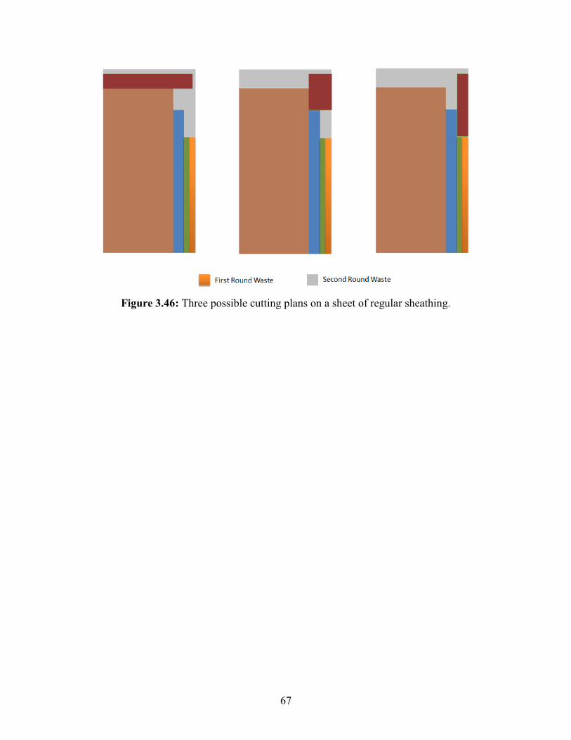
67
Figure 3.46: Three possible cutting plans on a sheet of regular sheathing.

68
Chapter 4 Case Study
4.1 Introduction
This section describes the case study implementations of the proposed
methodologies. Two in-house add-ons are developed based on Autodesk Revit to
perform the automation of quantity takeoff and material optimization. Two Revit
models from different companies are employed in the demonstration. First, the
material quantity in a model is extracted. Second, the lumber and sheathing usage
is optimized on the other model. Finally, the outputs of all work are exported, and
the results are analyzed.
4.2 Quantity Takeoff
4.2.1 Background
To illustrate the effectiveness of the proposed methodology, an actual case study
is presented. The case study demonstrates how the method is performed to extract
the material quantities from a 3D model in Revit, and the quantity takeoff is
displayed in the form of an Excel spreadsheet. The 3D model chosen to
demonstrate the quantity takeoff add-on is from a manufacturing plant in
Edmonton, Canada operated by Civeo (a modular construction manufacturer
specializing in modular workforce accommodations and camp logistics). The case
study object is a recreation facility 60 ft in length and 24 ft in width, achieved by
combining two 60 ft x 12 ft modules, and a common wall between the two
modules is removed to obtain a larger open space, and a staircase is installed
outside the module in order to provide access (Figure 4.1 and Figure 4.2).

69
Figure 4.1: 3D view of case study model.
Figure 4.2: Top view of case study model.
4.2.2 Preloading the Revit Model
This Revit model consists of two modules, and each is assigned a distinct Module
Number. The upper module in Figure 4.2 is assigned the Module Number Unit 02,
and the lower module is assigned the Module Number Unit 01. The materials
belonging to each module have the identical Module Number as the module.
Besides the modules, there is a staircase which is shared by the two modules, and

70
the staircase does not belong to any particular module, despite that it connects
with the Unit 01 module. The Module Number of the staircase is assigned as Site
Install. In this scenario, each material in the model has a 6-digit Part Number
(called JDE# in Civeo), and Module Number is named Unit Number, and the
combination of JDE# and Unit Number is the bridge to integrate the Revit model
with an Excel template and the key parameter to mirror the quantities onto the
Excel template (Figure 4.3).
Figure 4.3: Preloaded information in the Revit model.
4.2.3 Standardization of Excel Template
The material properties are transcribed into column headings in the Excel
template. This standardized Excel template contains the following columns,
Part_Number, Description1, Description2, Unit, and Unit_Number, which are
filled in advance of quantity extraction. Another two columns, Raw_Quantity and
Quantity are left blank to hold quantity extractions from Revit model.
Since three different units (Unit 01, Unit 02, and Site Install) exist in the model,
the content in the Excel template is duplicated twice, indicating that there are

71
three identical groups of materials that exist in the template, and Unit 01, Unit 02,
and Site Install are assigned to each group under the Unit_Number column (Table
4.1).
Table 4.1: Sample of Excel template (Unit_Number assignment).
4.2.4 Quantity Extraction
The quantity takeoff starts from an activation of the Quantity Takeoff add-on in
Revit (Figure 4.4).
Figure 4.4: Quantity takeoff interface (ExportToExcel).
The Excel template is chosen by clicking “Select File”, and the Excel template
file address is shown in the first textbox (Target Excel), and the sheet is selected
and the name is shown in the second textbox (Sheet Name). After the textboxes
are filled up, clicking the Export button activates the Quantity Takeoff, which
extracts the quantities from the Revit model to the Excel template.
In the Revit model, all the material information is collected, which includes the
Part Numbers, Unit Numbers, and Quantities. As long as more than one item has
Item_Number Quantity Unit Description1 Description2 Unit_Number Family_Name Raw_Quantity
009266 EA TABLE TENNIS Unit01
009266 EA TABLE TENNIS Unit02
009266 EA TABLE TENNIS Site Install

72
the same Part Number and Unit Number, they are grouped with a Quantity of the
sum. The prototype automatically searches the entire Excel template to sum up all
the cells matching with identical Part Number and Unit Number under the column
of Raw_Quantity. Due to the fact that formulas are preloaded into in the Excel
template, the column Raw_Quantity is filled with a number. Subsequently, the
number is modified by the formula and transported to the cell under the Quantity
column in the same row simultaneously. The final quantity takeoff output is
shown in Appendix E.
Table 4.2: Sample of extracted quantities.
The first two items (receptacle and switch) in the sample output belong to
Category 1, which is counted by each. Hence, the directly extracted quantity
under the column Raw_Quantity can be transferred to the Quantity column
without any processes. The third item (lumber 2x6x10 ft) and last item (Home
Wrap) belong to Category 2 and Category 3 respectively, so the formula is
required to transform the Raw Quantity.
𝑄 = 𝑄𝑅 ∗ 𝑓𝑢 ∗ (1 + 𝑓𝑤) ∗ (1 + 𝑓𝑐) (3.7)
For Category 2, it is uncontested to assume the extracted lumber length accords
with the final lumber length in real construction; as a result, the construction
factor 𝑓𝑐 is 0. However, the waste is inevitable due to the cutting process, and the
company always issues an extra 10% to 15% of materials for conservative
Item_Number Quantity Unit Description1 Description2 Unit_Number Raw_Quantity011830 6 EA RECP 15A 125V DUPLEX DECORA LEVITON 5325-W Unit 01 6
022319 2 EA SWITCH 15A 120V DECORA 3P WHITE LEVITON 5603-P2W Unit 01 2
004971 117.5966 EA LUM SPF 2X6X10FT #2&BTR Unit 01 1069.06
044566 0.594044 EA TYVEK HOME WRAP 10FT X 150FT Unit 01 645.7

73
estimate, which leads to the waste factor 𝑓𝑤 of 10% for lumber and other Category
2 materials. Moreover, since the unit piece of regular lumber is dimensioned by
10 ft, the unit conversion factor 𝑓𝑢 is set to be 1/10 to convert the extracted unit ft
to inventory unit Each. The final value after calculation is shown.
𝑄 = 1069.06 ∗ (1/10) ∗ (1 + 10%) ∗ (1 + 0) (3.7)
𝑄 = 117.60
As described in the previous section, the material waste from home wrap
placement on walls with openings is understandable and unavoidable, and the
waste causes the material quantity deviation between 3D model and reality;
therefore, the construction factor 𝑓𝑐 is evaluated to be 20% to eliminate the
measurement discrepancy. The stocked home wrap has dimensions of 10 ft x 150
ft (1,500 sq ft), so the unit conversion factor 𝑓𝑢 is set to be 1/1,500, and the waste
factor 𝑓𝑤is assumed to be 15%. Accordingly, the final formula is established
below.
𝑄 = 645.7 ∗ (1/1,500) ∗ (1 + 15%) ∗ (1 + 20%) (3.7)
𝑄 = 0.59
Dealing with over 10,000 items causes a high risk of error. Even if only one
number is typed incorrectly in the Revit model or Excel template, an unmatched
error will occur. To assist the add-on user to look up the incorrect items in a large
database, a dialog is designed for prompting errors. In the dialog, the incorrect
item types and the part numbers detected from Revit are displayed (Figure 4.5).
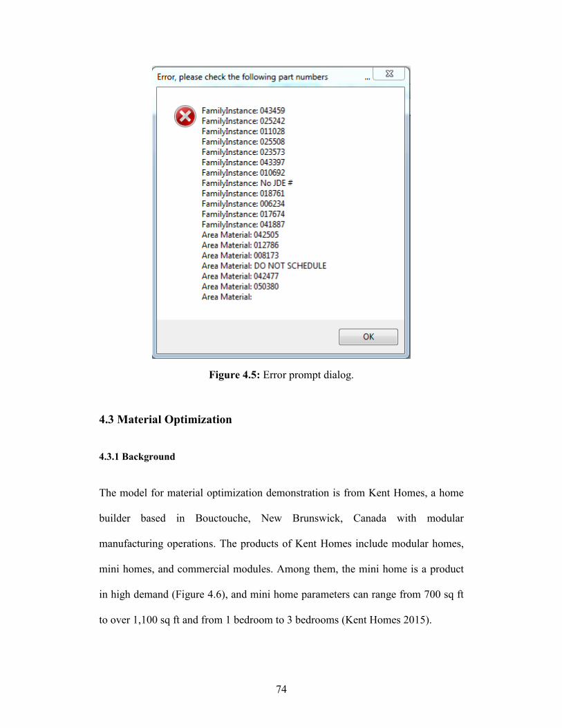
74
Figure 4.5: Error prompt dialog.
4.3 Material Optimization
4.3.1 Background
The model for material optimization demonstration is from Kent Homes, a home
builder based in Bouctouche, New Brunswick, Canada with modular
manufacturing operations. The products of Kent Homes include modular homes,
mini homes, and commercial modules. Among them, the mini home is a product
in high demand (Figure 4.6), and mini home parameters can range from 700 sq ft
to over 1,100 sq ft and from 1 bedroom to 3 bedrooms (Kent Homes 2015).
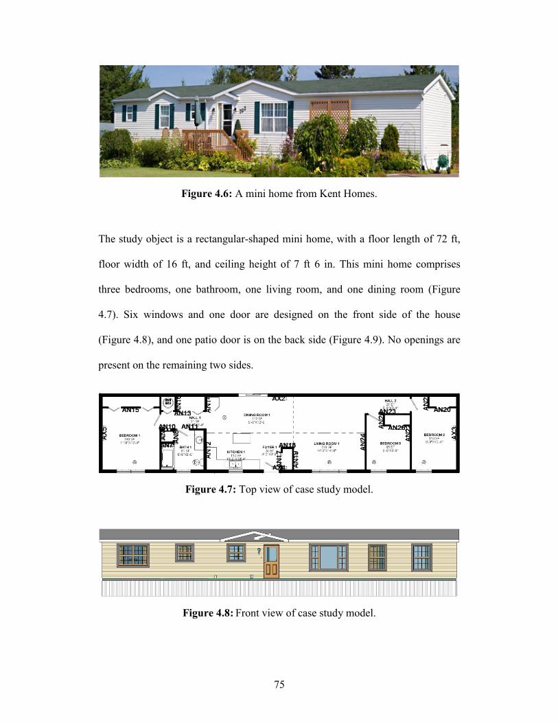
75
Figure 4.6: A mini home from Kent Homes.
The study object is a rectangular-shaped mini home, with a floor length of 72 ft,
floor width of 16 ft, and ceiling height of 7 ft 6 in. This mini home comprises
three bedrooms, one bathroom, one living room, and one dining room (Figure
4.7). Six windows and one door are designed on the front side of the house
(Figure 4.8), and one patio door is on the back side (Figure 4.9). No openings are
present on the remaining two sides.
Figure 4.7: Top view of case study model.
Figure 4.8: Front view of case study model.

76
Figure 4.9: Back view of case study model.
4.3.2 Lumber Optimization
The lumber optimization is performed by two algorithms, greedy and Simplex,
and both test the same model.
4.3.2.1 Preliminary Work
The precondition to optimize lumber usage is that the BIM model has completed
wall framing. However, the current Revit system does not offer a component to
represent lumber, so the model is framed by means of an external software called
StrucSoft MWF (Figure 4.10), developed by StrucSoft Solutions Ltd. StrucSoft
MWF is able to automate framing with wood studs in Revit (StrucSoft Solutions
2015). After this process, all the lumber is visible, and the information pertaining
to the lumber, such as nominal base dimensions, length, and volume, is also
accessible. What is notable is that properties are assigned to the lumber
simultaneously: BIMSF_Container, BIMSF_Description, and BIMSF_Label.
BIMSF_Container: the name of the host wall that lumber is framed into.
BIMSF_Description: the lumber type, decided by lumber location.
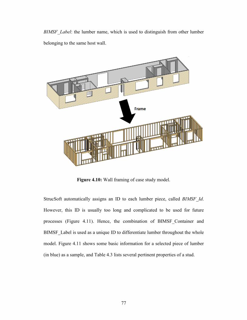
77
BIMSF_Label: the lumber name, which is used to distinguish from other lumber
belonging to the same host wall.
Figure 4.10: Wall framing of case study model.
StrucSoft automatically assigns an ID to each lumber piece, called BIMSF_Id.
However, this ID is usually too long and complicated to be used for future
processes (Figure 4.11). Hence, the combination of BIMSF_Container and
BIMSF_Label is used as a unique ID to differentiate lumber throughout the whole
model. Figure 4.11 shows some basic information for a selected piece of lumber
(in blue) as a sample, and Table 4.3 lists several pertinent properties of a stud.

78
Figure 4.11: Stud properties.
Table 4.3: Stud properties and naming rule.
Nominal Base
Dimension Length BIMSF_Container BIMSF_Description BIMSF_Label ID
2x6 7 ft 1 ½
in AX4 SV S10
AX4-
S10
As the precondition of wall framing is satisfied, the optimization commences. All
the lumber in the Revit model are collected and separated into different groups by
base dimension, and the lumber in each group is ranked by length and stored in a
corresponding virtual lumber pool for subsequent processes (see Appendix A, B,
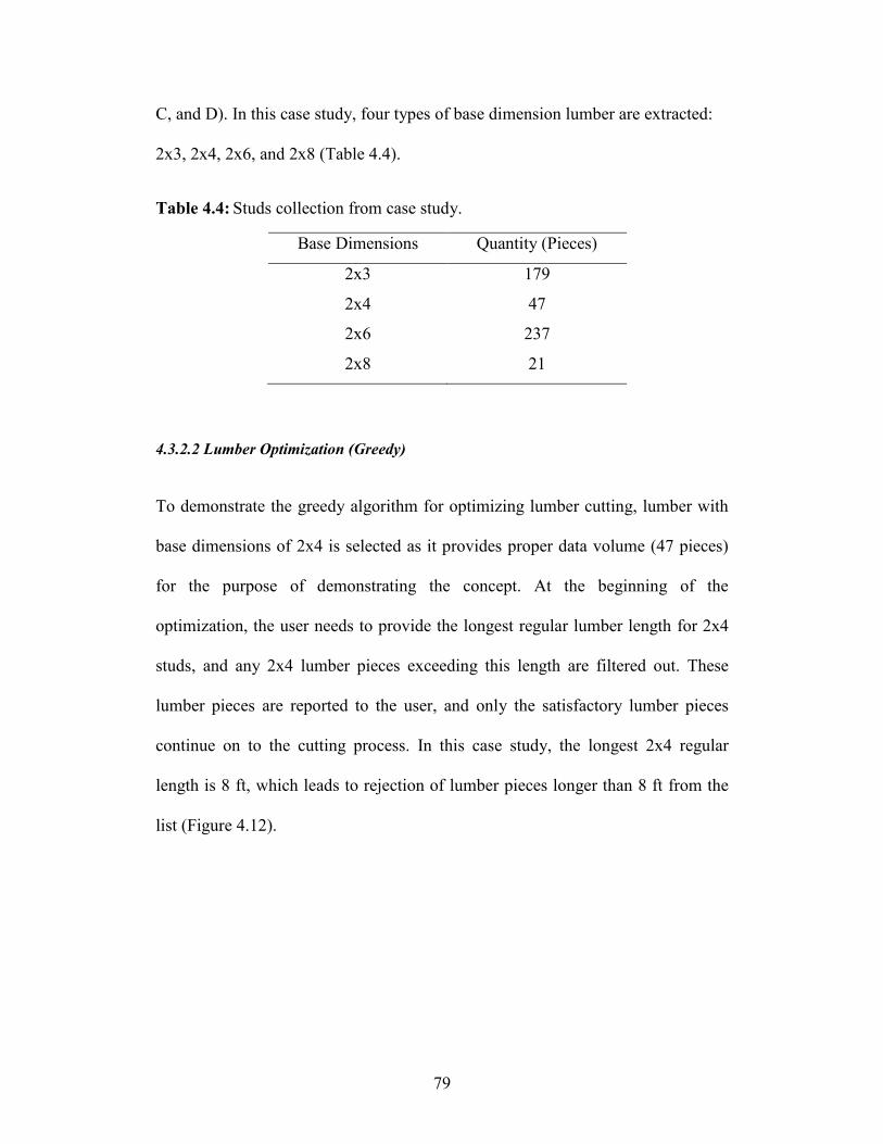
79
C, and D). In this case study, four types of base dimension lumber are extracted:
2x3, 2x4, 2x6, and 2x8 (Table 4.4).
Table 4.4: Studs collection from case study.
Base Dimensions Quantity (Pieces)
2x3 179
2x4 47
2x6 237
2x8 21
4.3.2.2 Lumber Optimization (Greedy)
To demonstrate the greedy algorithm for optimizing lumber cutting, lumber with
base dimensions of 2x4 is selected as it provides proper data volume (47 pieces)
for the purpose of demonstrating the concept. At the beginning of the
optimization, the user needs to provide the longest regular lumber length for 2x4
studs, and any 2x4 lumber pieces exceeding this length are filtered out. These
lumber pieces are reported to the user, and only the satisfactory lumber pieces
continue on to the cutting process. In this case study, the longest 2x4 regular
length is 8 ft, which leads to rejection of lumber pieces longer than 8 ft from the
list (Figure 4.12).
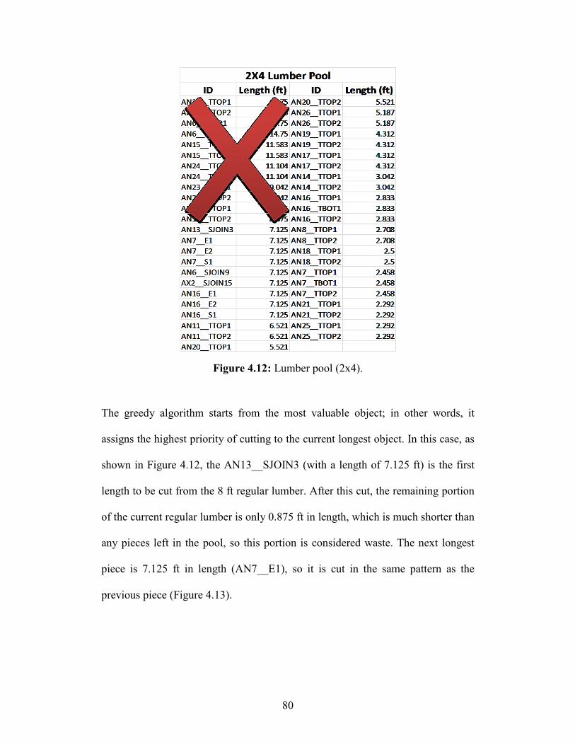
80
Figure 4.12: Lumber pool (2x4).
The greedy algorithm starts from the most valuable object; in other words, it
assigns the highest priority of cutting to the current longest object. In this case, as
shown in Figure 4.12, the AN13__SJOIN3 (with a length of 7.125 ft) is the first
length to be cut from the 8 ft regular lumber. After this cut, the remaining portion
of the current regular lumber is only 0.875 ft in length, which is much shorter than
any pieces left in the pool, so this portion is considered waste. The next longest
piece is 7.125 ft in length (AN7__E1), so it is cut in the same pattern as the
previous piece (Figure 4.13).

81
Figure 4.13: Lumber cutting (configuration 1).
Lumber pieces are cut in the one-piece-cut manner (only one piece cut from a
regular lumber) until AN20__TTOP1, which is 5.521 ft in length. After cutting
AN20__TTOP1 from the 8 ft regular lumber, the remaining portion is 2.479 ft in
length. It can be used to cut the longest remaining piece whose length is less than
2.479 ft, which is AN7__TTOP1 (2.458 ft). Afterwards, the remaining lumber
portion is only 0.021 ft in length, which is considered waste (Figure 4.14, left).
Two regular lumbers are used for cutting in this manner, and AN26__TTOP1
becomes the greatest length (5.187 ft). After cutting this piece, the remaining
2.813 ft can be used for the next longest piece, which is AN8__TTOP1 (2.708 ft)
(Figure 4.14).

82
Figure 4.14: Lumber cutting (configuration 2).
The next two-piece combinations are 4.312 ft + 3.042 ft (0.646 ft waste) (Figure
4.15, left), and 4.312 ft + 2.833 ft (0.855 ft waste) (Figure 4.15, right).
Figure 4.15: Lumber cutting (configuration 3).
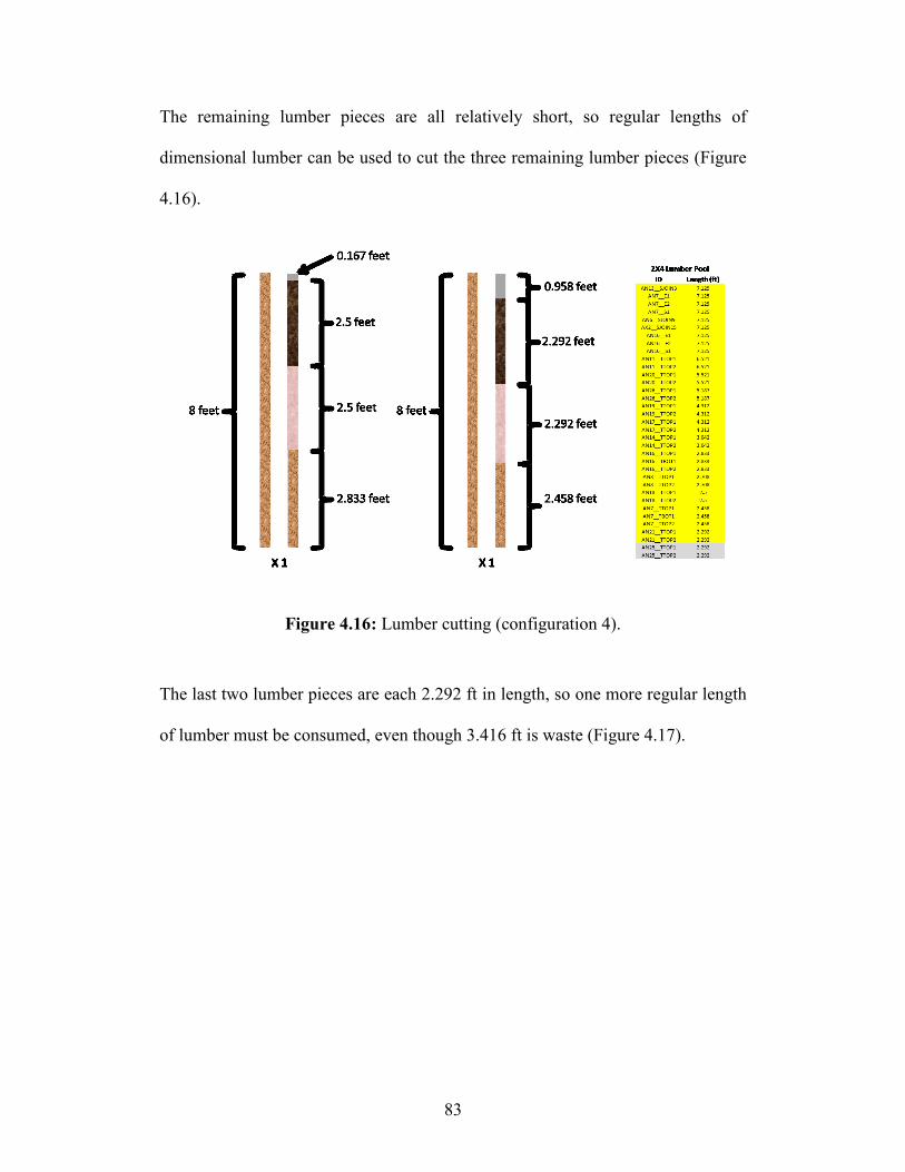
83
The remaining lumber pieces are all relatively short, so regular lengths of
dimensional lumber can be used to cut the three remaining lumber pieces (Figure
4.16).
Figure 4.16: Lumber cutting (configuration 4).
The last two lumber pieces are each 2.292 ft in length, so one more regular length
of lumber must be consumed, even though 3.416 ft is waste (Figure 4.17).

84
Figure 4.17: Lumber cutting (configuration 5).
4.3.2.3 Lumber Optimization (Simplex)
The Simplex algorithm permits the user to utilize multiple lengths of regular
lumber; (in this research, the interface is designed to accept up to three lengths of
regular lumber from the end user). For each regular lumber, the user needs to
assign a unit value or cost to each regular lumber length. It is not necessary to be a
real cost, as the purpose is to create a cost relationship between different regular
lumber lengths. To demonstrate the Simplex algorithm, the 2x6 lumber group is
tested, and three different lengths of 2x6 regular lumber, 8 ft, 10 ft, and 12 ft, are
supplied. The market prices are assumed to be $8/piece, $10/piece, and $12/piece,
respectively. In this situation, the value spaces can be filled with 8, 10, 12, or 4, 5,
6 (Figure 4.18).

85
OR
Figure 4.18: Lumber optimization interface (lumber information input).
As mentioned above, the over-dimensioned lumber pieces are filtered out based
on the criterion of the longest regular lumber among the provided regular lumber
lengths. In this case study, the filter removes the lumber pieces longer than 12 ft.
The remaining lumber pieces are grouped by length and ranked in descending
order (Table 4.5). The optimization is transformed to a linear program with matrix
representation, which contains an objective function, target array, coefficient
matrix, coefficient variables, and decision variables.
Table 4.5: Grouped lumber pool (2x6).
2x6 Lumber
Rank Length (ft) Quantity
1 8.062 3
2 7.167 2
3 7.125 159
4 6.771 2
5 6.708 2
6 6.521 12

86
7 6.188 3
8 5.833 2
9 3.333 4
10 3.25 8
11 3 4
12 2.562 3
13 2.25 6
14 1.333 15
It is easy to obtain the Target Array, which is an array that contains the quantities
in descending sequence of lumber piece length.
Target Array = [3, 2, 159, 2, 2, 12, 3, 2, 4, 8, 4, 3, 6, 15]
Although the coefficient matrix is complex to build, a feasible approach is the
integration of the tree structure and greedy algorithm. In this case study, 14 levels
are used in the tree structure ranking, where each level represents a required cut
length from a piece of regular lumber. The higher the ranking on the list, the
longer the length of the piece to be cut; in other words, the longest piece is located
at the highest tree level, and the shortest piece is located at the lowest tree level.
The strategy is to obtain the first cutting pattern by cutting the longest piece and
then the next longest piece from the list that is shorter than the remaining portion
of current regular lumber after the first cut; continue this pattern constantly until
the remaining portion of the regular lumber is shorter than any lengths remaining
to be cut; this remaining portion is regarded as waste, as it is too short to satisfy
any other lengths. Transpose the quantities of lumber pieces to be cut at each level

87
into a corresponding array. After obtaining the first array, the second one can be
derived from it. The method is: go through all the elements in the first array; if
there is any non-zero element not located at the lowest tree structure level, select
the lowest-level element, and reduce the value of the element by one without
modifying any elements higher than this level; implement the tree structure again
from this level until a full piece of regular lumber is only used to cut the shortest
pieces.
In this case study, the first length of regular lumber is 12 ft. The first piece in the
2x6 lumber pool is 8.062 ft in length, so the quantity of 8.062 ft is cut from a 12 ft
length of regular lumber and is represented by a value of 1 in the array, which is
projected to the first element of the first array. The second lumber length that can
be cut from the remaining portion (3.938 ft) is 3.333 ft, which is located at level
nine, and the quantity is also given a value of 1, so that the ninth element in the
first array is 1. After cutting the 3.333 ft, the regular lumber has only 0.605 ft
remaining, which is too short to be used for any other cut. Hence, the first array is:
Array1 (12 ft) = [1, 0, 0, 0, 0, 0, 0, 0, 1, 0, 0, 0, 0, 0]
This array signifies that a regular length of lumber (12 ft in length) is used to cut
one lumber piece of 8.062 ft in length and another lumber piece of 3.333 ft in
length.
After checking all the elements in the first array, the first and ninth elements are
found to be non-zero. Since the ninth element is located at a lower level on the
tree structure, the value of the element (1) is reduced by 1, which becomes 0. The

88
tree structure method is implemented again starting from this level (level nine) to
generate the second array.
Array2 (12 ft) = [1, 0, 0, 0, 0, 0, 0, 0, 0, 1, 0, 0, 0, 0]
By such analogy, a list of arrays is created, and each array represents one cutting
pattern. The last array has only one non-zero element, which is the last level, and
once this level is reached, all the cutting patterns have been exhausted.
ArrayN (12 ft) = [0, 0, 0, 0, 0, 0, 0, 0, 0, 0, 0, 0, 0, 9]
All the cutting patterns (N patterns) of a 12 ft regular length of lumber are shown
below.
[1, 0, 0, 0, 0, 0, 0, 0, 1, 0, 0, 0, 0, 0]
[1, 0, 0, 0, 0, 0, 0, 0, 0, 1, 0, 0, 0, 0]
[0, 0, 0, 0, 0, 0, 0, 0, 0, 0, 0, 0, 1, 7]
[0, 0, 0, 0, 0, 0, 0, 0, 0, 0, 0, 0, 0, 9]
The coefficient matrix (14 x N) for the regular lumber (12 ft in length):

89
Decision Variables Array is an array with N unknowns, and each unknown
represents how many 12 ft regular lengths of lumber are used to cut the
corresponding certain pattern.
Decision Variable Array = [𝑛1, 𝑛2, 𝑛3, 𝑛4, 𝑛5, 𝑛6 …… 𝑛𝑁−2, 𝑛𝑁−1, 𝑛𝑁]
Coefficient Variable Array is an array with N constants, and these constants are
the values read from the user interface. Since the current example is 12 ft regular
lumber, all of the N constants are 12 (There is only one regular length in this
situation, so the value can be any positive number as long as they are identical).
Coefficient Variable Array = [12, 12, 12, 12 … … 12, 12, 12, 12]
The optimization goal is to minimize the total cost of consumed regular lumber,
so the objective function is minimizing the dot product of Decision Variables
Array and Coefficient Variable Array.
Minimize: Decision Variables Array * Coefficient Variable Array
Minimize: 12 ∗ 𝑛1 + 12 ∗ 𝑛2 + 12 ∗ 𝑛3 + 12 ∗ 𝑛4 + ⋯ + 12 ∗ 𝑛𝑁−2 + 12 ∗ 𝑛𝑁−1 + 12 ∗ 𝑛𝑁
Based on the relationship of
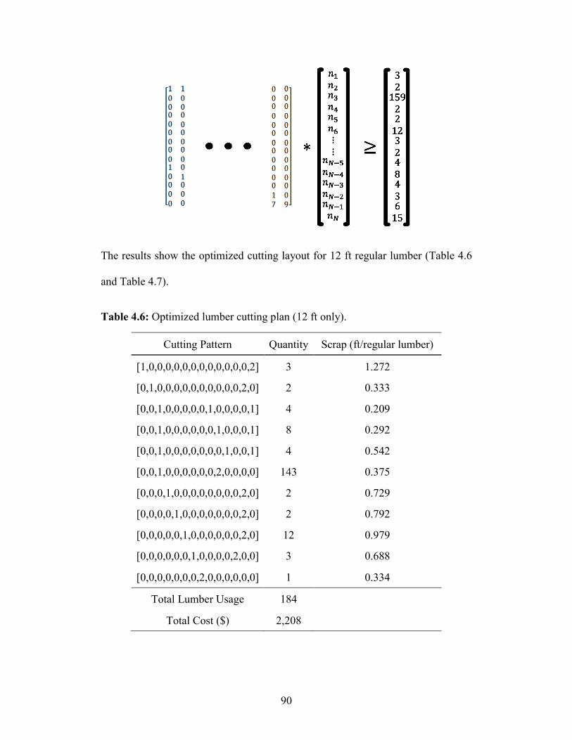
90
The results show the optimized cutting layout for 12 ft regular lumber (Table 4.6
and Table 4.7).
Table 4.6: Optimized lumber cutting plan (12 ft only).
Cutting Pattern Quantity Scrap (ft/regular lumber)
[1,0,0,0,0,0,0,0,0,0,0,0,0,2] 3 1.272
[0,1,0,0,0,0,0,0,0,0,0,0,2,0] 2 0.333
[0,0,1,0,0,0,0,0,1,0,0,0,0,1] 4 0.209
[0,0,1,0,0,0,0,0,0,1,0,0,0,1] 8 0.292
[0,0,1,0,0,0,0,0,0,0,1,0,0,1] 4 0.542
[0,0,1,0,0,0,0,0,0,2,0,0,0,0] 143 0.375
[0,0,0,1,0,0,0,0,0,0,0,0,2,0] 2 0.729
[0,0,0,0,1,0,0,0,0,0,0,0,2,0] 2 0.792
[0,0,0,0,0,1,0,0,0,0,0,0,2,0] 12 0.979
[0,0,0,0,0,0,1,0,0,0,0,2,0,0] 3 0.688
[0,0,0,0,0,0,0,2,0,0,0,0,0,0] 1 0.334
Total Lumber Usage 184
Total Cost ($) 2,208

91
Table 4.7: Optimized lumber cutting result (12 ft only).
2x6 Lumber (12 ft)
Rank Length (ft) Required Quantity Actual Quantity
1 8.062 3 3
2 7.167 2 2
3 7.125 159 159
4 6.771 2 2
5 6.708 2 2
6 6.521 12 12
7 6.188 3 3
8 5.833 2 2
9 3.333 4 4
10 3.250 8 8
11 3.000 4 4
12 2.562 3 6
13 2.250 6 22
14 1.333 15 22
By performing the same method, the results of optimized cutting layout for 10 ft
regular lumber are shown in Table 4.8 and Table 4.9.

92
Table 4.8: Optimized lumber cutting plan (10 ft only).
Cutting Pattern Quantity Scrap (ft/regular lumber)
[1,0,0,0,0,0,0,0,0,0,0,0,0,1] 3 0.605
[0,1,0,0,0,0,0,0,0,0,0,0,1,0] 2 0.583
[0,0,1,0,0,0,0,0,0,0,0,0,1,0] 153 0.625
[0,0,1,0,0,0,0,0,0,0,0,0,0,2] 6 0.209
[0,0,0,1,0,0,0,0,0,0,0,0,1,0] 2 0.979
[0,0,0,0,1,0,0,0,0,0,0,1,0,0] 2 0.730
[0,0,0,0,0,1,0,0,1,0,0,0,0,0] 2 0.146
[0,0,0,0,0,1,0,0,0,1,0,0,0,0] 6 0.229
[0,0,0,0,0,1,0,0,0,0,1,0,0,0] 4 0.479
[0,0,0,0,0,0,1,0,0,1,0,0,0,0] 2 0.562
[0,0,0,0,0,0,1,0,0,0,0,1,0,0] 1 1.250
[0,0,0,0,0,0,0,1,1,0,0,0,0,0] 2 0.834
Total Lumber Usage 185
Total Cost ($) 1,850

93
Table 4.9: Optimized lumber cutting result (10 ft only).
2x6 Lumber (10 ft)
Rank Length (ft) Required Quantity Actual Quantity
1 8.062 3 3
2 7.167 2 2
3 7.125 159 159
4 6.771 2 2
5 6.708 2 2
6 6.521 12 12
7 6.188 3 3
8 5.833 2 2
9 3.333 4 4
10 3.250 8 8
11 3.000 4 4
12 2.562 3 3
13 2.250 6 157
14 1.333 15 15
The 8 ft regular lumber is also an option for cutting, but the longest piece length
in the 2x6 Lumber Pool is 8.062 ft, which is longer than 8 ft, and is not feasible by
using 8 ft regular lumber only. However, if all of the 8.062 ft lumber pieces are
ignored and the 8 ft regular lumber is used to produce the lumber pieces with
lengths shorter than 8 ft, the result is shown below (Table 4.10 and Table 4.11).

94
Table 4.10: Optimized lumber cutting plan (8 ft only).
Cutting Pattern Quantity Scrap (ft/regular lumber)
[0,1,0,0,0,0,0,0,0,0,0,0,0,0] 2 0.833
[0,0,1,0,0,0,0,0,0,0,0,0,0,0] 159 0.875
[0,0,0,1,0,0,0,0,0,0,0,0,0,0] 2 1.229
[0,0,0,0,1,0,0,0,0,0,0,0,0,2] 2 1.292
[0,0,0,0,0,1,0,0,0,0,0,0,0,1] 12 0.146
[0,0,0,0,0,0,1,0,0,0,0,0,0,1] 3 0.479
[0,0,0,0,0,0,0,1,0,0,0,0,0,1] 2 0.834
[0,0,0,0,0,0,0,0,2,0,0,0,0,1] 2 0.001
[0,0,0,0,0,0,0,0,1,2,0,0,0,0] 3 0.167
[0,0,0,0,0,0,0,0,0,1,0,0,2,0] 2 0.250
[0,0,0,0,0,0,0,0,0,0,2,0,0,1] 1 0.667
[0,0,0,0,0,0,0,0,0,0,1,1,1,0] 3 0.188
Total Lumber Usage 193
Total Cost ($) 1,544
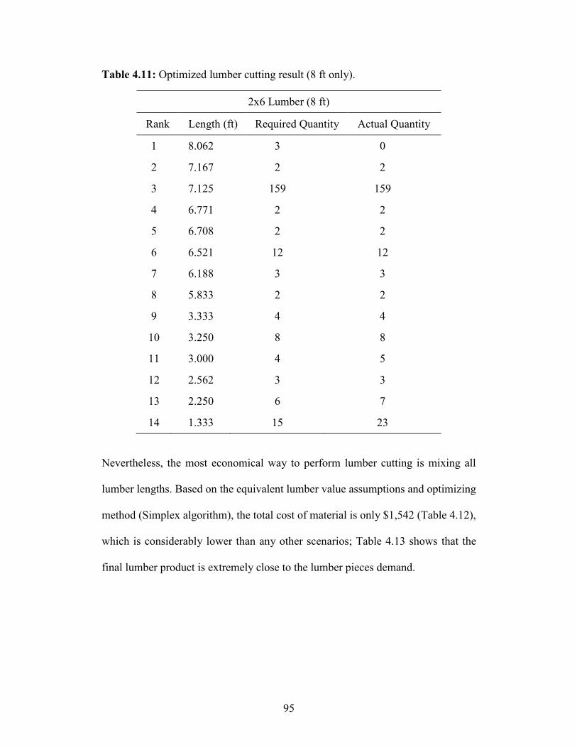
95
Table 4.11: Optimized lumber cutting result (8 ft only).
2x6 Lumber (8 ft)
Rank Length (ft) Required Quantity Actual Quantity
1 8.062 3 0
2 7.167 2 2
3 7.125 159 159
4 6.771 2 2
5 6.708 2 2
6 6.521 12 12
7 6.188 3 3
8 5.833 2 2
9 3.333 4 4
10 3.250 8 8
11 3.000 4 5
12 2.562 3 3
13 2.250 6 7
14 1.333 15 23
Nevertheless, the most economical way to perform lumber cutting is mixing all
lumber lengths. Based on the equivalent lumber value assumptions and optimizing
method (Simplex algorithm), the total cost of material is only $1,542 (Table 4.12),
which is considerably lower than any other scenarios; Table 4.13 shows that the
final lumber product is extremely close to the lumber pieces demand.
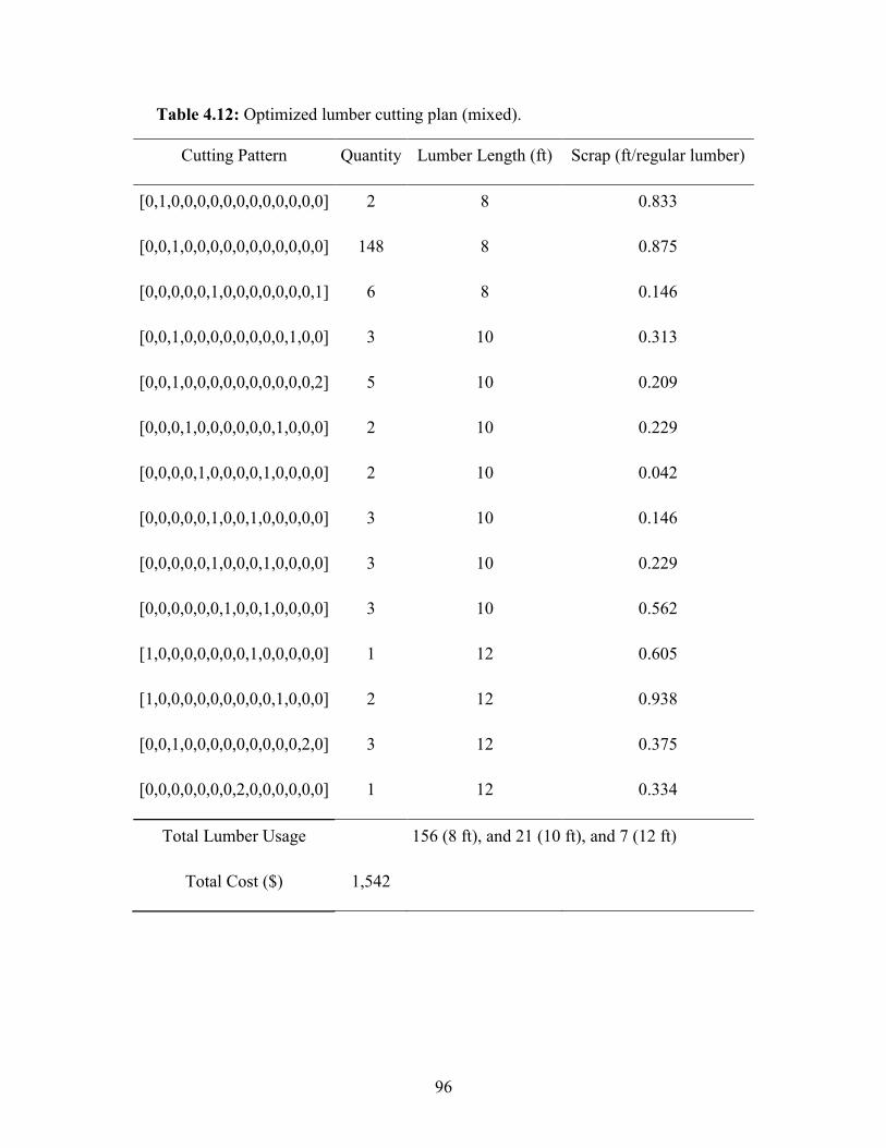
96
Table 4.12: Optimized lumber cutting plan (mixed).
Cutting Pattern Quantity Lumber Length (ft) Scrap (ft/regular lumber)
[0,1,0,0,0,0,0,0,0,0,0,0,0,0] 2 8 0.833
[0,0,1,0,0,0,0,0,0,0,0,0,0,0] 148 8 0.875
[0,0,0,0,0,1,0,0,0,0,0,0,0,1] 6 8 0.146
[0,0,1,0,0,0,0,0,0,0,0,1,0,0] 3 10 0.313
[0,0,1,0,0,0,0,0,0,0,0,0,0,2] 5 10 0.209
[0,0,0,1,0,0,0,0,0,0,1,0,0,0] 2 10 0.229
[0,0,0,0,1,0,0,0,0,1,0,0,0,0] 2 10 0.042
[0,0,0,0,0,1,0,0,1,0,0,0,0,0] 3 10 0.146
[0,0,0,0,0,1,0,0,0,1,0,0,0,0] 3 10 0.229
[0,0,0,0,0,0,1,0,0,1,0,0,0,0] 3 10 0.562
[1,0,0,0,0,0,0,0,1,0,0,0,0,0] 1 12 0.605
[1,0,0,0,0,0,0,0,0,0,1,0,0,0] 2 12 0.938
[0,0,1,0,0,0,0,0,0,0,0,0,2,0] 3 12 0.375
[0,0,0,0,0,0,0,2,0,0,0,0,0,0] 1 12 0.334
Total Lumber Usage 156 (8 ft), and 21 (10 ft), and 7 (12 ft)
Total Cost ($) 1,542

97
Table 4.13: Optimized lumber cutting result (mixed).
2x6 Lumber (mixed)
Rank Length (ft) Required Quantity Actual Quantity
1
2
3
4
5
6
7
8
9
10
11
12
13
14
8.062
7.167
7.125
6.771
6.708
6.521
6.188
5.833
3.333
3.250
3.000
2.562
2.250
1.333
3
2
159
2
2
12
3
2
4
8
4
3
6
15
3
2
159
2
2
12
3
2
4
8
4
3
6
16
The lumber cutting pattern, quantity, and label are all available at this stage, and a
framing layout (Figure 4.19) can be exported from Revit, so the lumber cutting
and framing processes can easily be connected by lumber labels.
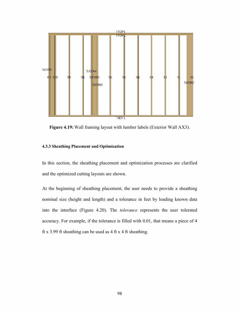
98
Figure 4.19: Wall framing layout with lumber labels (Exterior Wall AX3).
4.3.3 Sheathing Placement and Optimization
In this section, the sheathing placement and optimization processes are clarified
and the optimized cutting layouts are shown.
At the beginning of sheathing placement, the user needs to provide a sheathing
nominal size (height and length) and a tolerance in feet by loading known data
into the interface (Figure 4.20). The tolerance represents the user tolerated
accuracy. For example, if the tolerance is filled with 0.01, that means a piece of 4
ft x 3.99 ft sheathing can be used as 4 ft x 4 ft sheathing.

99
Figure 4.20: Sheathing placement and optimization interface.
4.3.3.1 Sheathing Placement
To demonstrate the sheathing placement function, two sheathing sizes are tested,
4x8 (4 ft in length and 8 ft in height) and 4x7 (4 ft in length and 7 ft in height).
The sheathing of 4x8 is higher than the wall height in the case study, which is 7 ft
6 in. The other (4x7) is shorter than the wall height. Six windows and one door
are on the house’s front wall (wall label: AX4), which is the most complicated
face compared to the other 3 wall faces, so the case study focuses on this wall,
which is 72 ft in length and 7 ft 6 in in height.
Case 1 (Sheathing size: 4x8)
As mentioned in the methodology, to start placing sheathing on a wall, the first
step is to identify the Framing Point (Figure 4.21) based on the wall layer
thicknesses (Figure 4.22) and the coordinates of the pertinent points at the corner.
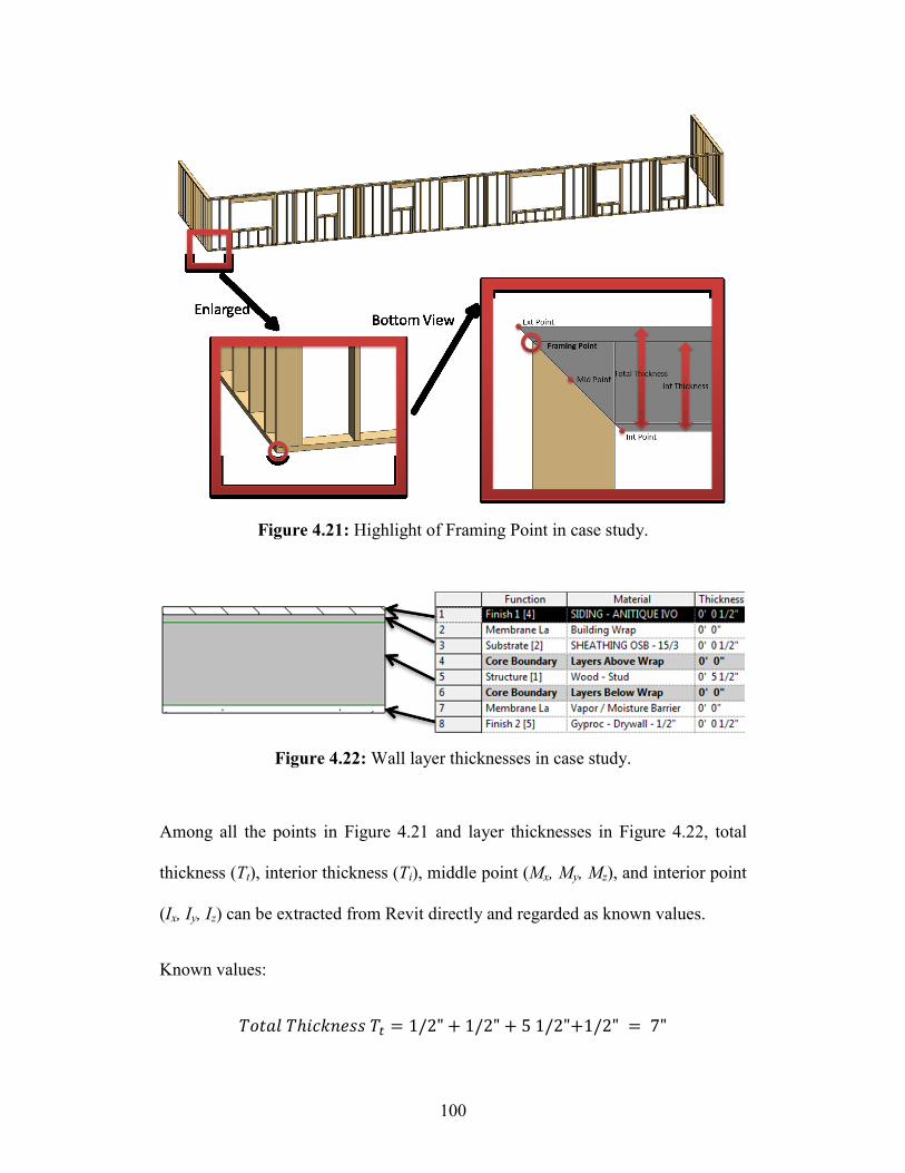
100
Figure 4.21: Highlight of Framing Point in case study.
Figure 4.22: Wall layer thicknesses in case study.
Among all the points in Figure 4.21 and layer thicknesses in Figure 4.22, total
thickness (Tt), interior thickness (Ti), middle point (Mx, My, Mz), and interior point
(Ix, Iy, Iz) can be extracted from Revit directly and regarded as known values.
Known values:
𝑇𝑜𝑡𝑎𝑙 𝑇ℎ𝑖𝑐𝑘𝑛𝑒𝑠𝑠 𝑇𝑡 = 1/2" + 1/2" + 5 1/2"+1/2" = 7"

101
𝐼𝑛𝑡𝑒𝑟𝑖𝑜𝑟 𝑇ℎ𝑖𝑐𝑘𝑛𝑒𝑠𝑠 𝑇𝑖 = 5 1/2"+1/2" = 6"
𝐼𝑛𝑡𝑒𝑟𝑖𝑜𝑟 𝑃𝑜𝑖𝑛𝑡 (𝐼𝑥, 𝐼𝑦, 𝐼𝑧) = (−40′ 5 43/128", 6′ 9 39/64", 0′ 0")
𝑀𝑖𝑑𝑑𝑙𝑒 𝑃𝑜𝑖𝑛𝑡 (𝑀𝑥, 𝑀𝑦, 𝑀𝑧) = (−40′ 8 107/128", 6′ 6 7/64", 0′ 0")
After substituting the known values for the components in the following
functions, the result of Framing Point (𝐹𝑥 , 𝐹𝑦, 𝐹𝑧) is accessible.
𝐹𝑥 = 𝐼𝑥 +2×(𝑀𝑥−𝐼𝑥)
𝑇𝑡× 𝑇𝑖 (3.11)
𝐹𝑦 = 𝐼𝑦 +2×(𝑀𝑦−𝐼𝑦)
𝑇𝑡× 𝑇𝑖 (3.12)
𝐹𝑧 = 𝐼𝑧 = 𝑀𝑧 = 0 (3.13)
𝐹𝑥 = −40′ 5 43/128" +2 × (−40′ 8 107/128" − (−40′ 5 43/128"))
7"
× 6"=-40' 11 43/128"
𝐹𝑦 = 6′ 9 39/64" +2 × (6′ 6 7/64" − 6′ 9 39/64")
7"× 6" = 6′ 3 39/64"
𝐹𝑧 = 0′ 0" = 0′ 0" = 0′ 0"
𝐹𝑟𝑎𝑚𝑖𝑛𝑔 𝑃𝑜𝑖𝑛𝑡 (𝐹𝑥, 𝐹𝑦, 𝐹𝑧) = (−40′ 11 43/128", 6′ 3 39/64", 0′ 0")
As the Framing Point is available, the next values to be calculated for sheathing
placement are the length and height of sheathing. The sheathing length is
determined dealing with two conditions:
𝑙𝑖 = {𝐷1, 𝐷1 ≤ 𝐿𝑅
𝐷2, 𝐷1 > 𝐿𝑅 (3.20)
𝐷1: Distance between the current Start Point and the closest Group 1 End Point
following the wall direction.

102
𝐷2: Distance between the current Start Point and the furthest Group 2 End Point
following the wall direction, where distance always has a value less than the
regular sheathing length (4 ft).
As the Figure 4.23 shows, 𝐷1 of this wall framing is obviously 2 ft 10 ½ in, which
is shorter than𝐿𝑅 4 ft. Therefore, the length of the first piece of sheathing (𝑙1) is 2
ft 10 ½ in.
For the sheathing height, since the regular sheathing size in this case study is 4 by
8 (height (𝐻𝑅): 8 ft), only one piece of regular sheathing is sufficient to cover the
whole wall height (𝐻𝑤), 7 ft 6 in. Hence the first piece of sheathing height (ℎ1) is
7 ft 6 in.
Figure 4.23: Framing Point and three possible sheathing lengths in the wall
framing.

103
As Figure 4.24 illustrates, installation of the first sheathing piece onto the wall
generates the Start Points for subsequent pieces above and below the window
framing and the piece for full wall-height framing on the other side of the window
opening. Both of the sheathing lengths are equal to the width of the window frame
(5 ft 10 in), which can be extracted directly from the model, and the heights are
equal to the framing above and below the window opening, and the equations to
calculate the values are recalled here:
Sheathing height above the ith
window:
ℎ𝑖 = 𝐻𝑤 − 𝑇𝑠𝑏𝑝 − 𝐻𝑤𝑗𝑖 = 7′6" − 1 1/2" − 6′6 1/4" = 10 1/4"
Sheathing height below the ith
window:
ℎ𝑖 = 𝐻𝑤𝑐𝑖 + 𝑇𝑠𝑏𝑝 + 𝑇𝑑𝑠𝑝𝑖 = 2′3+1 1/2 + 3" = 2′7 1/2"
The bottom sheathing piece has a length of 5 ft 10 in and a height of 2 ft 7½ in,
and the top sheathing piece has a length of 5 ft 10 in and a height of 10 ¼ in. To
calculate the Start Points, the wall direction is a key value. In this case study, the
wall is drawn along the x-axis from negative to positive, which generates the wall
vector of (1,0,0).
Start Point 1:
𝑃𝑥 = (𝑙𝑖 + 𝑊𝑤𝑖) ∗ 𝑟𝑥 + 𝑝𝑥 = (2′10 1/2" + 5′10") ∗ 1 + (−40′ 11 43/128")
= −31′ 9 43/128"
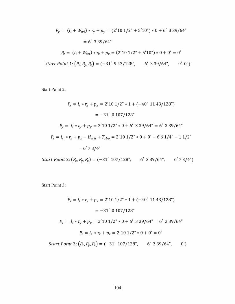
104
𝑃𝑦 = (𝑙𝑖 + 𝑊𝑤𝑖) ∗ 𝑟𝑦 + 𝑝𝑦 = (2′10 1/2" + 5′10") ∗ 0 + 6′ 3 39/64"
= 6′ 3 39/64"
𝑃𝑧 = (𝑙𝑖 + 𝑊𝑤𝑖) ∗ 𝑟𝑧 + 𝑝𝑧 = (2′10 1/2" + 5′10") ∗ 0 + 0′ = 0′
𝑆𝑡𝑎𝑟𝑡 𝑃𝑜𝑖𝑛𝑡 1: (𝑃𝑥, 𝑃𝑦 , 𝑃𝑧) = (−31′ 9 43/128", 6′ 3 39/64", 0′ 0")
Start Point 2:
𝑃𝑥 = 𝑙𝑖 ∗ 𝑟𝑥 + 𝑝𝑥 = 2′10 1/2" ∗ 1 + (−40′ 11 43/128")
= −31′ 0 107/128"
𝑃𝑦 = 𝑙𝑖 ∗ 𝑟𝑦 + 𝑝𝑦 = 2′10 1/2" ∗ 0 + 6′ 3 39/64" = 6′ 3 39/64"
𝑃𝑧 = 𝑙𝑖 ∗ 𝑟𝑧 + 𝑝𝑧 + 𝐻𝑤𝑗𝑖 + 𝑇𝑠𝑏𝑝 = 2′10 1/2" ∗ 0 + 0′ + 6′6 1/4" + 1 1/2"
= 6′ 7 3/4"
𝑆𝑡𝑎𝑟𝑡 𝑃𝑜𝑖𝑛𝑡 2: (𝑃𝑥, 𝑃𝑦 , 𝑃𝑧) = (−31′ 107/128", 6′ 3 39/64", 6′ 7 3/4")
Start Point 3:
𝑃𝑥 = 𝑙𝑖 ∗ 𝑟𝑥 + 𝑝𝑥 = 2′10 1/2" ∗ 1 + (−40′ 11 43/128")
= −31′ 0 107/128"
𝑃𝑦 = 𝑙𝑖 ∗ 𝑟𝑦 + 𝑝𝑦 = 2′10 1/2" ∗ 0 + 6′ 3 39/64" = 6′ 3 39/64"
𝑃𝑧 = 𝑙𝑖 ∗ 𝑟𝑧 + 𝑝𝑧 = 2′10 1/2" ∗ 0 + 0′ = 0′
𝑆𝑡𝑎𝑟𝑡 𝑃𝑜𝑖𝑛𝑡 3: (𝑃𝑥 , 𝑃𝑦, 𝑃𝑧) = (−31′ 107/128", 6′ 3 39/64", 0′)

105
Figure 4.24: Three Start Points are created.
The Start Point at the right bottom corner of the bottom sheathing piece enables
the following placements (Figure 4.25). Formula 3.20 is recalled here to
determine the lengths of sheathing pieces.
𝑙𝑖 = {𝐷1, 𝐷1 ≤ 𝐿𝑅
𝐷2, 𝐷1 > 𝐿𝑅 (3.20)
𝐷2 = 6′1 1/2", which is longer than regular sheathing length(𝐿𝑅 = 4′), so 𝑙𝑖 is
equal to 𝐷1 = 3′3 1/2" in this situation. The consecutive sheathing piece’s length
is equal to𝐷2 = 2′10". Since the wall height is less than the regular sheathing
height, both of the heights are the same as the wall height, which is 7’6”.

106
Figure 4.25: Sheathing placements in case study.
With the methodology utilized to place the previous pieces of sheathing, the
whole wall panel is framed by sheathing, and Figure 4.26 shows the front view of
the external wall (AX4) with completed sheathing placement (4x8 regular
sheathing). After the placement, each piece of sheathing has a label assigned at
the centre, and the format is the combination of “AX4-S” and sheathing ID, which
is a digit.
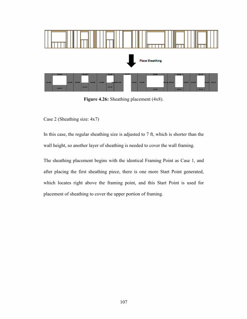
107
Figure 4.26: Sheathing placement (4x8).
Case 2 (Sheathing size: 4x7)
In this case, the regular sheathing size is adjusted to 7 ft, which is shorter than the
wall height, so another layer of sheathing is needed to cover the wall framing.
The sheathing placement begins with the identical Framing Point as Case 1, and
after placing the first sheathing piece, there is one more Start Point generated,
which locates right above the framing point, and this Start Point is used for
placement of sheathing to cover the upper portion of framing.
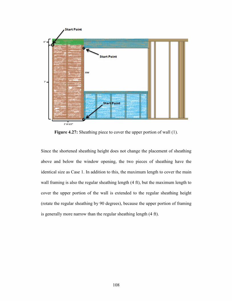
108
Figure 4.27: Sheathing piece to cover the upper portion of wall (1).
Since the shortened sheathing height does not change the placement of sheathing
above and below the window opening, the two pieces of sheathing have the
identical size as Case 1. In addition to this, the maximum length to cover the main
wall framing is also the regular sheathing length (4 ft), but the maximum length to
cover the upper portion of the wall is extended to the regular sheathing height
(rotate the regular sheathing by 90 degrees), because the upper portion of framing
is generally more narrow than the regular sheathing length (4 ft).
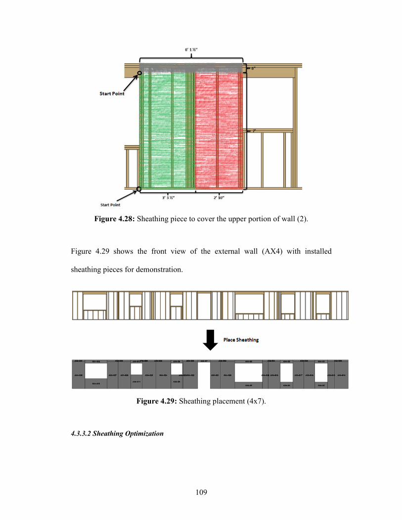
109
Figure 4.28: Sheathing piece to cover the upper portion of wall (2).
Figure 4.29 shows the front view of the external wall (AX4) with installed
sheathing pieces for demonstration.
Figure 4.29: Sheathing placement (4x7).
4.3.3.2 Sheathing Optimization

110
The sheathing pieces in Sheathing Placement Case 1 (sheathing nominal size:
height = 8 ft, length = 4 ft) are selected for the sheathing optimization
demonstration, and stored in a virtual sheathing pool. The sheathing pieces are
assigned different labels and ranked first by height and then by length; a
Sheathing Piece Pool is formed (Table 4.14).
Table 4.14: Sheathing pieces collection.
The first step of the sheathing optimization is checking the sheathing in the pool;
as long as the current longest piece (7 ft 6 in) is higher than the regular sheathing
length (4 ft), the regular sheathing is orientated vertically, otherwise, it is
orientated horizontally.
The cutting always starts from the highest ranking piece (AX2—S3) at bottom left
corner. Since the length of regular sheathing is fulfilled, after cutting the first
piece, only the top portion of sheathing remains, which has 4 ft in height and 0.5
ft in length (Figure 4.30). After going through all the sheathing pieces remaining
Rank Label Length (ft) Height (ft) Rank Label Length (ft) Height (ft) Rank Label Length (ft) Height (ft)
1 AX2--S3 4 7.5 19 AX4--S24 3.9384 7.5 37 AX4--S21 2.6042 7.5
2 AX2--S4 4 7.5 20 AX2--S5 3.9166 7.5 38 AX4--S15 1.8126 7.5
3 AX2--S7 4 7.5 21 AX4--S20 3.8556 7.5 39 AX2--S9 1.5536 7.5
4 AX2--S8 4 7.5 22 AX4--S22 3.8528 7.5 40 AX4--S19 1.5 7.5
5 AX2--S11 4 7.5 23 AX3--S1 3.6666 7.5 41 AX4--S23 0.1875 7.5
6 AX2--S12 4 7.5 24 AX5--S1 3.6666 7.5 42 AX4--S6 1.7188 7.1666
7 AX2--S13 4 7.5 25 AX2--S2 3.5402 7.5 43 AX4--S5 0.8542 7.1666
8 AX2--S14 4 7.5 26 AX4--S14 3.5402 7.5 44 AX2--S1 0.6666 5.9376
9 AX2--S15 4 7.5 27 AX4--S25 3.5 7.5 45 AX4--S13 2.6354 5.8334
10 AX2--S16 4 7.5 28 AX4--S28 3.3334 7.5 46 AX4--S12 0.8542 5.8334
11 AX2--S17 4 7.5 29 AX4--S26 3.3126 7.5 47 AX4--S11 3 3.6354
12 AX2--S18 4 7.5 30 AX2--S10 3.1756 7.5 48 AX4--S9 3 3.6354
13 AX3--S2 4 7.5 31 AX4--S18 3.1458 7.5 49 AX4--S2 1.7188 3.3334
14 AX3--S3 4 7.5 32 AX2--S19 3.125 7.5 50 AX4--S4 1.7188 3.3334
15 AX3--S4 4 7.5 33 AX4--S16 2.8542 7.5 51 AX4--S1 0.8542 3.3334
16 AX5--S2 4 7.5 34 AX4--S17 2.8542 7.5 52 AX4--S3 0.8542 3.3334
17 AX5--S3 4 7.5 35 AX4--S27 2.8124 7.5 53 AX4--S7 1.125 3.2084
18 AX5--S4 4 7.5 36 AX2--S6 2.75 7.5 54 AX4--S8 0.8542 3
55 AX4--S10 0.8542 3
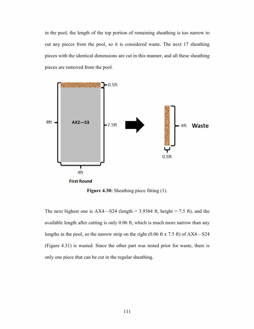
111
in the pool, the length of the top portion of remaining sheathing is too narrow to
cut any pieces from the pool, so it is considered waste. The next 17 sheathing
pieces with the identical dimensions are cut in this manner, and all these sheathing
pieces are removed from the pool.
Figure 4.30: Sheathing piece fitting (1).
The next highest one is AX4—S24 (length = 3.9384 ft, height = 7.5 ft), and the
available length after cutting is only 0.06 ft, which is much more narrow than any
lengths in the pool, so the narrow strip on the right (0.06 ft x 7.5 ft) of AX4—S24
(Figure 4.31) is wasted. Since the other part was tested prior for waste, there is
only one piece that can be cut in the regular sheathing.

112
Figure 4.31: Sheathing piece fitting (2).
The same cutting pattern is repeated for the next three pieces until AX3—S1 is
reached, because on the right side of AX3—S1, there is sufficient space to fit
another piece of sheathing, which is AX4—S23 (Figure 4.32).

113
Figure 4.32: Sheathing piece fitting (3).
In this case study, most of the regular sheathing can cut only one or two pieces
side by side vertically, as previously shown. In addition, another three cutting
patterns are available.
After cutting the piece AX4—S13 from a regular sheathing (Figure 4.33), there
are no other pieces that can be cut from the remaining portion on the right side of
AX4—S13, so it is waste. Upon testing the upper remaining portion, it is found
that it can be used to cut AX4—S2.

114
Figure 4.33: Sheathing piece fitting (4).
As shown in Figure 4.34, after cutting two pieces (AX4—S17 and AX4—S1) on a
regular sheathing, three rectangular portions remain, and after testing each of
them, one rectangular portion can be used to cut AX4—S23.
Figure 4.34: Sheathing piece fitting (5).
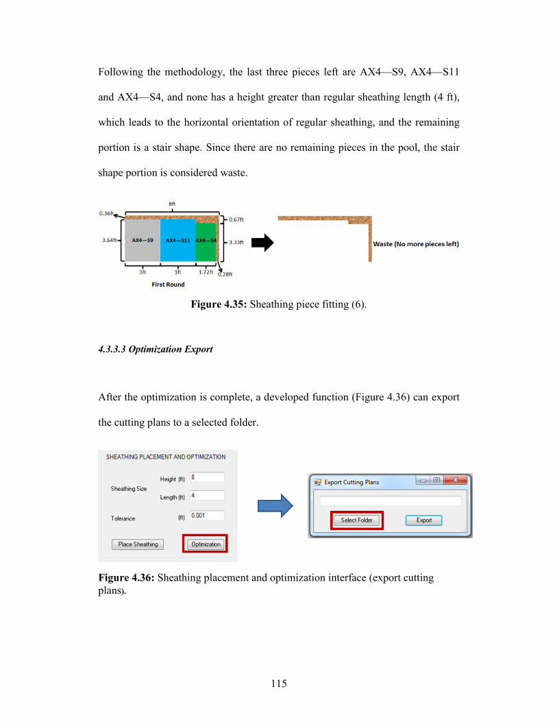
115
Following the methodology, the last three pieces left are AX4—S9, AX4—S11
and AX4—S4, and none has a height greater than regular sheathing length (4 ft),
which leads to the horizontal orientation of regular sheathing, and the remaining
portion is a stair shape. Since there are no remaining pieces in the pool, the stair
shape portion is considered waste.
Figure 4.35: Sheathing piece fitting (6).
4.3.3.3 Optimization Export
After the optimization is complete, a developed function (Figure 4.36) can export
the cutting plans to a selected folder.
Figure 4.36: Sheathing placement and optimization interface (export cutting
plans).
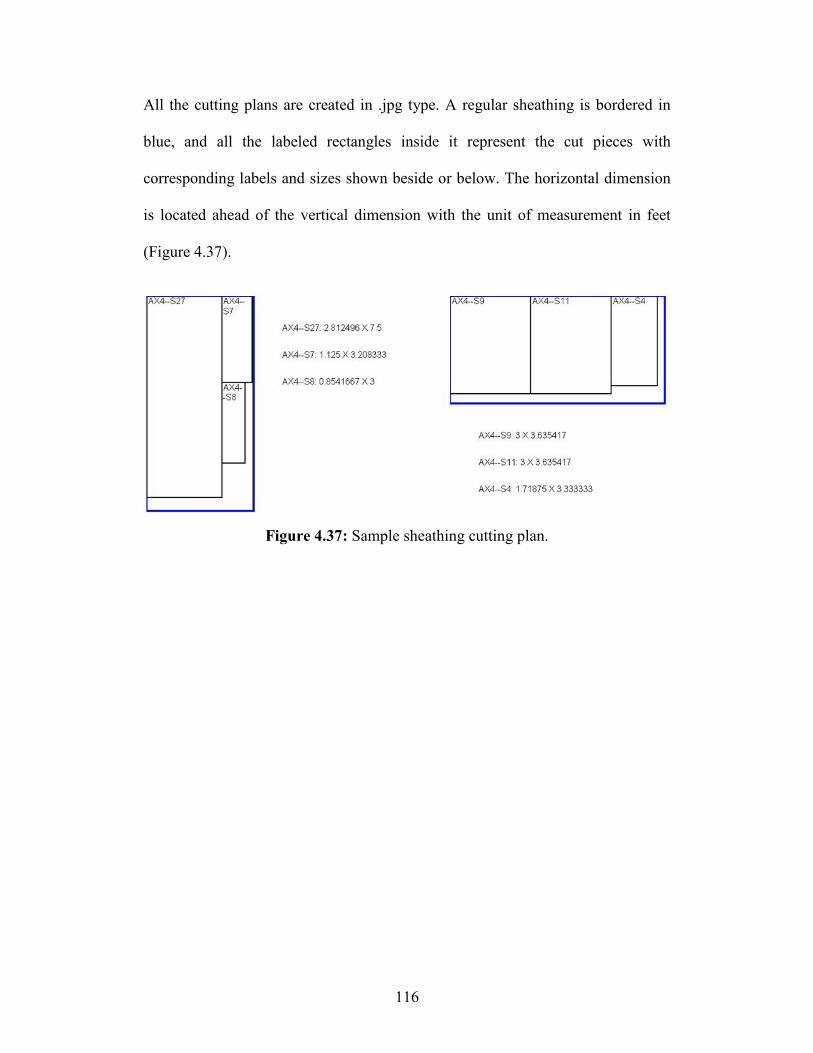
116
All the cutting plans are created in .jpg type. A regular sheathing is bordered in
blue, and all the labeled rectangles inside it represent the cut pieces with
corresponding labels and sizes shown beside or below. The horizontal dimension
is located ahead of the vertical dimension with the unit of measurement in feet
(Figure 4.37).
Figure 4.37: Sample sheathing cutting plan.

117
Chapter 5 Conclusion
5.1 General Conclusion
This thesis presents methodologies for quantity takeoff and material optimization,
and they are implemented by two user interfaces developed in the environment of
Microsoft Visual C#.NET and embedded into Autodesk Revit.
The task of quantity takeoff is time-consuming and error prone. It currently
employs a 2D print-out from a graphical environment, and the main processes,
including material counting, measurement, and calculation, are carried out
manually rather than by computer. Hence, the research is motivated by the need
for an automated quantity takeoff system embedded in Autodesk Revit, which
will allow the operation to be performed quickly and accurately, and will limit
human error. The final output is an Excel file containing all the necessary
quantities.
Material optimization is developed in order to optimize the usage of 1D material
(lumber) and 2D material (sheathing). The greedy algorithm and simplex
algorithm are applied to optimize lumber, and greedy and Bottom-Left Heuristic
algorithms are the main strategies employed for sheathing optimization. The end-
user of the add-on need only provide nominal sizes of lumber and sheathing, and
the program is able to provide relatively optimized cutting scenarios for the wall
sheathing layout to increase workers’ productivity and reduce material waste. The
final output also provides practical material quantities for inventory.

118
5.2 Research Contributions
The developed programs in this research, including quantity takeoff and material
optimization, can benefit the current modular construction industry in many
respects. These benefits are outlined below.
5.2.1 Quantity Takeoff
• The developed quantity takeoff can decrease operation time from
approximately 150 minutes to less than 30 seconds, which represents a
99% time savings; this progress can also limit the potential for and effect
of human error.
• Since the automated quantity takeoff time is extremely efficient compared
to the current manual process, the time requirement to update takeoff due
to any unforeseen changes in the construction plan is also decreased
significantly.
5.2.2 Material Optimization
• Visualization of sheathing on walls provides a good sense of how the work
can be performed efficiently and reduces the experience requirement of
sheathing framers to a relatively low level.
• Optimization of materials gives carpenters a clear cutting plan by showing
the cutting lengths and quantities; it not only decreases material waste but
also increases productivity by eliminating guesswork in the process.

119
• Cutting plans and lumber/sheathing framing plans are distributed to
workers of different trades, but the plans can be connected by labels on
each item. Hence the productivity is improved by avoiding errors in
communication between different trades.
5.3 Research Limitations
• The precondition of quantity takeoff is that, the Revit model needs to be
preloaded with classification system information. For any modular
construction company, this is a time-consuming task due to a large amount
of input items; even the slightest error in the input process, such as an extra
space or an incorrect digit, can greatly affect the outcome.
• The quantity takeoff program cannot offer feasible 1D and 2D material
quantities due to limitations of the Revit model, which could not consider
the material cutting process, but only read the total length (1D materials)
and net area (2D materials).
• The lumber optimization can be performed by the greedy algorithm and
Simplex algorithm. Each algorithm has some limitations:
o For the greedy algorithm, only one length for each nominal size of
lumber can be used for cutting; therefore, it will not be the most
economical method.

120
o Simplex algorithm can accommodate multiple lengths of lumber;
however, an external library (for example, IBM CPLEX Optimizer)
is required.
• Since the greedy algorithm is also applied to sheathing optimization, only
one sheathing size can be used for optimization.
• The developed program only allows for one type of sheathing to be used in
a given project.
5.4 Future Improvement
These research methodologies can serve as the foundation for quantity takeoff and
material optimization, and at least the following three improvements can be
implemented in the future:
• Apply multiple sheathing sizes with Simplex algorithm for optimization.
• Apply multiple sheathing types (regular and fire-rated sheathing) for
optimization.
• The sheathing placement function currently only works on vertical
placement, so the function can be improved to cover other sheathing
placement patterns.

121
References
Aryanezhad, M. B., Fakhim Hashemi, N., Makui, A., and Javanshir, H. (2012).
“A simple approach to the two-dimensional guillotine cutting stock
problem.” Journal of Industrial Engineering International, 8(21).
Autodesk (2008). “BIM and API Extensions.” Retrieved April 20, 2015, from
http://images.autodesk.com/latin_am_main/files/revit_bim_and_api_extensio
ns_mar08.pdf
Autodesk (2013). “Lesson 3: Model-Based Estimating and Quantity Takeoff.”
Retrieved November 18, 2014, from
http://bimcurriculum.autodesk.com/lesson/lesson-3-model-based-estimating-
and-quantity-takeoff
Beyond the Paper (2006). “What is quantity takeoff?” Retrieved November 18,
2014, from
http://dwf.blogs.com/beyond_the_paper/2006/04/what_is_quantit.html
Build Your Own House (2015). “Laying Concrete Slabs and Framing your
House” Retrieved February 26, 2015, from
http://buildyourhouse.blog.com/2011/05/30/laying-concrete-slabs-framing-
your-house/
Building Information Modeling (2014). Retrieved November 19, 2014, from
http://eds.b.ebscohost.com/eds/ebookviewer/ebook/bmxlYmtfXzc2MDc5M
V9fQU41?sid=3d7e9e39-e638-479b-aac9-
761e5d590298@sessionmgr113andvid=5andformat=EBandrid=2
Costa, F. M. and Sassi R. J. (2012). “Application of an hybrid bio-inspired meta-
heuristic in the optimization of two-dimensional guillotine cutting in an glass
industry.” Intelligent Data Engineering and Automated Learning - IDEAL
2012 (7435), 802–809.

122
Firat, C. E., Arditi, D., Hamalainen, J.-P., Stenstrand, J., and Kiiras, J. (2010)
“Quantity take-off in model-based systems.” Proceedings of the CIB W78
2010: 27th International Conference, Nov. 16–18.
Home Innovation Research Labs (2001). “Residential construction waste: From
disposal to management.” Retrieved January 26, 2015, from
http://www.toolbase.org/Best-Practices/Construction-Waste/residential-
construction-waste
Insulation Online (2014). “Tyvek Housewrap Breather Membrane.” Retrieved
February 2, 2015, from http://www.just-insulation.com/002-brands/tyvek-
housewrap-breather-membrane-for-walls.html
Kent Homes (2015). “Mini Homes.” Retrieved January 30, 2015, from
http://www.kenthomes.com/kent-homes-browse-mini-
homes.aspx?HomeStyle=Mini%20Homes
Macleod, B. (1993). “An algorithm for the 2D guillotine cutting stock problem.”
European Journal of Operational Research, 68(3), 400-412.
Mah, D. and Al-Hussein, M. (2008). “Residential construction material waste
minimization analysis during the framing stage.” Proceedings, Canadian
Society for Civil Engineering Annual Conference, Québec City, QC, Canada,
Jun. 10-13, 417-425.
Manrique, J. D., Al-Hussein, M., Bouferguene, A., Safouhi, H., and Nasseri, R.
(2011). “Combinatorial algorithm for optimizing wood waste in framing
designs.” Journal of Construction Engineering and Management, 137(3),
188–197.
Manrique, J. D. and Juan, D. (2009). “Automation of design and drafting for
wood frame structures and construction waste minimization.” Automation in
Construction, (55), 15-24.
Monteiro, A. and Poças Martins, J. (2013). “A survey on modeling guidelines for
quantity takeoff-oriented BIM-based design.” Automation in Construction,
35, 238–253.

123
Pekin Hardwood (2015). “Lumber.” Retrieved February 26, 2015, from
http://www.pekinhardwood.com/lumber
Sabol, L. (2008). “Challenges in cost estimating with building information
modeling.” Design + Construction Strategy, 1–16.
StrucSoft Solutions (2015). “MWF.” Retrieved February 19, 2015, from
http://strucsoftsolutions.com/products/
Van Nederveen, G. A. and Tolman, F. P. (1992). “Modelling multiple views on
buildings.” Automation in Construction, 1(3), 215–224.

124
Appendices
A: 2x3 lumber pool

125
B: 2x4 lumber pool

126
C: 2x6 lumber pool
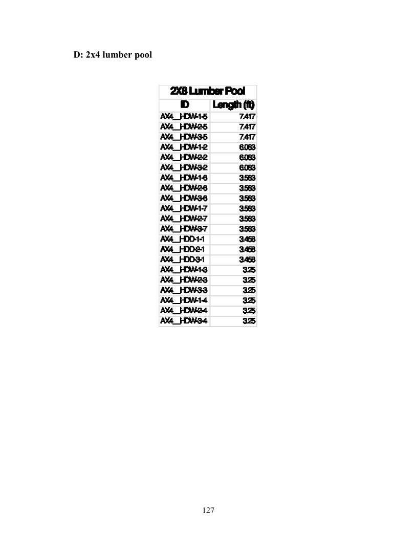
127
D: 2x4 lumber pool
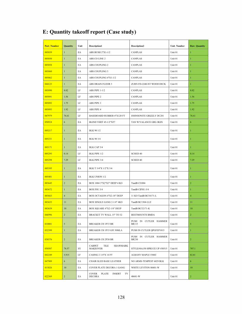
128
E: Quantity takeoff report (Case study)
Part_Number Quantity Unit Description1 Description2 Unit_Number Raw_Quantity
005039 1 EA ABS BUSH 2"X1-1/2 CANPLAS Unit 01 1
005050 1 EA ABS CO LINE 2 CANPLAS Unit 01 1
005058 1 EA ABS COUPLING 2 CANPLAS Unit 01 1
005060 1 EA ABS COUPLING 3 CANPLAS Unit 01 1
005062 1 EA ABS COUPLING 4"X1-1/2 CANPLAS Unit 01 1
044123 1 EA ABS DRAIN FLOOR 3 ZURN FD-2240-NT WOOD DECK Unit 01 1
005090 8.02 LF ABS PIPE 1-1/2 CANPLAS Unit 01 8.02
005091 1.56 LF ABS PIPE 2 CANPLAS Unit 01 1.56
005092 1.75 LF ABS PIPE 3 CANPLAS Unit 01 1.75
005093 1.92 LF ABS PIPE 4 CANPLAS Unit 01 1.92
047979 76.61 LF BASEBOARD RUBBER 4"X120 FT JOHNSONITE GRIZZLY DC281 Unit 01 76.61
050918 6 EA BLIND VERT 45-1/2"X57 TAN W/VALANCE GRG JKSN Unit 01 6
005217 1 EA BLK 90 1/2 Unit 01 1
005231 1 EA BLK 90 3/4 Unit 01 1
005171 1 EA BLK CAP 3/4 Unit 01 1
005295 0.14 LF BLK PIPE 1/2 SCHED 40 Unit 01 0.14
005298 7.29 LF BLK PIPE 3/4 SCHED 40 Unit 01 7.29
005395 1 EA BLK T 3/4"X 1/2"X 3/4 Unit 01 1
005401 1 EA BLK UNION 1/2 Unit 01 1
003645 2 EA BOX 1004 3"X2"X3" DEEP 4 KO TandB CI1004 Unit 01 2
003672 1 EA BOX FSU 3/4 TandB CIFSU-3/4 Unit 01 1
003663 4 EA BOX OCTAGON 4"X2-18" DEEP 11 KO TandB BC54171-L Unit 01 4
003653 11 EA BOX SINGLE GANG 2-1/4" 4KO TandB BC1504-LLE Unit 01 11
003659 10 EA BOX SQUARE 4"X2-1/8" DEEP TandB BC52171-K Unit 01 10
046996 2 EA BRACKET TV WALL 15" TO 32 BESTMOUNTS BMDA Unit 01 2
010001 5 EA BREAKER CH 1P15 BR PUSH IN CUTLER HAMMER
BR115 Unit 01 5
032399 1 EA BREAKER CH 1P15 GFI 30MLA PUSH IN CUTLER QPGFEP1015 Unit 01 1
030376 2 EA BREAKER CH 2P30 BR PUSH IN CUTLER HAMMER
BR230 Unit 01 2
050507 78.57 SY CARPET TILE SHAWMARK
MAKEOVER STYLE#0A150 SPRUCE UP #50515 Unit 01 707.1
042249 5.915 LF CASING 2 1/4"X 14 FT ALBANY MAPLE #3002 Unit 01 82.81
047909 6 EA CHAIR SLED BASE LEATHER NO ARMS-TEMPEST 6029 BLK Unit 01 6
015826 10 EA COVER PLATE DECORA 1 GANG WHITE LEVITON 80401-W Unit 01 10
022369 2 EA COVER PLATE INSERT TV
DECORA 40681-W Unit 01 2
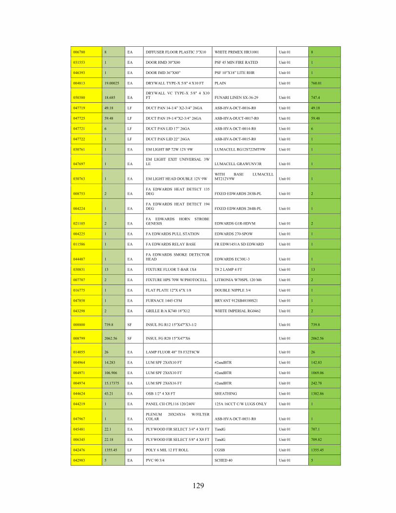
129
006780 8 EA DIFFUSER FLOOR PLASTIC 3"X10 WHITE PRIMEX HR31001 Unit 01 8
031553 1 EA DOOR HMD 30"X80 PSF 45 MIN FIRE RATED Unit 01 1
046393 1 EA DOOR IMD 36”X80” PSF 10”X18” LITE RHR Unit 01 1
004813 19.00025 EA DRYWALL TYPE-X 5/8" 4 X10 FT PLAIN Unit 01 760.01
050380 18.685 EA DRYWALL VC TYPE-X 5/8" 4 X10
FT FUNARI LINEN SX-36-29 Unit 01 747.4
047719 49.18 LF DUCT PAN 14-1/4” X2-3/4” 26GA ASB-HVA-DCT-0016-R0 Unit 01 49.18
047725 59.48 LF DUCT PAN 19-1/4”X2-3/4” 26GA ASB-HVA-DUCT-0017-R0 Unit 01 59.48
047721 6 LF DUCT PAN LID 17” 26GA ASB-HVA-DCT-0014-R0 Unit 01 6
047722 1 LF DUCT PAN LID 22” 26GA ASB-HVA-DCT-0015-R0 Unit 01 1
030761 1 EA EM LIGHT BP 72W 12V 9W LUMACELL RG12S722MT9W Unit 01 1
047697 1 EA EM LIGHT EXIT UNIVERSAL 3W
LE LUMACELL GRAWUNV3R Unit 01 1
030763 1 EA EM LIGHT HEAD DOUBLE 12V 9W WITH BASE LUMACELL
MT212V9W Unit 01 1
008753 2 EA FA EDWARDS HEAT DETECT 135
DEG FIXED EDWARDS 283B-PL Unit 01 2
004224 1 EA FA EDWARDS HEAT DETECT 194
DEG FIXED EDWARDS 284B-PL Unit 01 1
021105 2 EA FA EDWARDS HORN STROBE
GENESIS EDWARDS G1R-HDVM Unit 01 2
004225 1 EA FA EDWARDS PULL STATION EDWARDS 270-SPOW Unit 01 1
011586 1 EA FA EDWARDS RELAY BASE FR EDW1451A SD EDWARD Unit 01 1
044487 1 EA FA EDWARDS SMOKE DETECTOR
HEAD EDWARDS EC30U-3 Unit 01 1
030831 13 EA FIXTURE FLUOR T-BAR 1X4 T8 2 LAMP 4 FT Unit 01 13
007707 2 EA FIXTURE HPS 70W W/PHOTOCELL LITHONIA W70SPL 120 M6 Unit 01 2
016775 1 EA FLAT PLATE 12"X 6"X 1/8 DOUBLE NIPPLE 3/4 Unit 01 1
047858 1 EA FURNACE 1445 CFM BRYANT 912SB48100S21 Unit 01 1
043298 2 EA GRILLE R/A K740 18"X12 WHITE IMPERIAL RG0462 Unit 01 2
008800 739.8 SF INSUL FG R12 15"X47"X3-1/2 Unit 01 739.8
008799 2062.56 SF INSUL FG R20 15"X47"X6 Unit 01 2062.56
014055 26 EA LAMP FLUOR 48" T8 F32T8CW Unit 01 26
004964 14.283 EA LUM SPF 2X4X10 FT #2andBTR Unit 01 142.83
004971 106.906 EA LUM SPF 2X6X10 FT #2andBTR Unit 01 1069.06
004974 15.17375 EA LUM SPF 2X6X16 FT #2andBTR Unit 01 242.78
044624 43.21 EA OSB 1/2" 4 X8 FT SHEATHING Unit 01 1382.86
044219 1 EA PANEL CH CPL116 120/240V 125A 16CCT C/W LUGS ONLY Unit 01 1
047967 1 EA PLENUM 20X24X16 W/FILTER
COLAR ASB-HVA-DCT-0031-R0 Unit 01 1
045481 22.1 EA PLYWOOD FIR SELECT 3/4" 4 X8 FT TandG Unit 01 707.1
006345 22.18 EA PLYWOOD FIR SELECT 5/8" 4 X8 FT TandG Unit 01 709.82
042476 1355.45 LF POLY 6 MIL 12 FT ROLL CGSB Unit 01 1355.45
042983 5 EA PVC 90 3/4 SCHED 40 Unit 01 5

130
012785 6.49 LF PVC PIPE 3/4 SCHED 40 BELL END Unit 01 6.49
032474 6 EA PVC S636 90 3 ULC APPROVED FOR VENTING Unit 01 6
026886 14.43 LF PVC S636 PIPE 3 Unit 01 14.43
011830 6 EA RECP 15A 125V DUPLEX DECORA LEVITON 5325-W Unit 01 6
004194 2 EA RECP 15A 125V DUPLEX GFI LEVITON N7599-W Unit 01 2
046993 709.82 EA ROOF DECTEC R15000 13 FT X 62
FT EMBOSSED WHITE 806 SF/RL Unit 01 709.82
051414 1 EA SLEEVE GALV 24"X12"X4-1/2 W/1" FLANGE ONE END Unit 01 1
022319 2 EA SWITCH 15A 120V DECORA 3P WHITE LEVITON 5603-P2W Unit 01 2
009275 1 EA TABLE POOL W/TRI CUE BALL SET CANADA BILLIARDS 0203 Unit 01 1
009266 1 EA TABLE TENNIS Unit 01 1
042841 1 EA TABLE TEXAS HOLDEM POKER Unit 01 1
009091 1 EA TAPIN CIRCULAR GALV 6 Unit 01 1
040653 2 EA TV 32 Unit 01 2
044566 645.7 LF TYVEK HOME WRAP 10 FT X 150 FT Unit 01 645.7
014901 1 EA VALVE BALL PVC 3/4 SCHED 40 ECONOMY Unit 01 1
045945 6 EA WINDOW PVC 47-1/4"X59-3/8 SEALED JAMB 6-3/4 Unit 01 6
Unknown10 1 _PTI FLOOR OPENING MEP FLOOR OPENING Unit 01 1
Unknown19 1 48100 furnace assembly 48100 furnace assembly Unit 01 1
Unknown20 1 COIL AC 4 TON=CNPVP4821ALA Coil=simplify Unit 01 1
Unknown21 1 MEP ROOF OPENING MEP ROOF OPENING Unit 01 1
Unknown23 4 J152 mwfW_PanelJoin Unit 01 4
Unknown26 6 PanelParams PanelParams Unit 01 6
Unknown27 1 J153 mwfW_PanelJoin Unit 01 1
Unknown28 1 J163 mwfW_PanelJoin Unit 01 1
Unknown29 8 2x6 BIMSF-Dimension Lumber Unit 01 8
Unknown32 1 24x24 - 6x6 Neck Supply Diffuser - Rectangular Face Unit 01 1
047979 79.12 LF BASEBOARD RUBBER 4"X120 FT JOHNSONITE GRIZZLY DC281 Unit 02 79.12
050918 7 EA BLIND VERT 45-1/2"X57 TAN W/VALANCE GRG JKSN Unit 02 7
046996 2 EA BRACKET TV WALL 15" TO 32 BESTMOUNTS BMDA Unit 02 2
047808 1 EA CAP END 19-1/4"X2-3/4" 26GA ASB-HVA-DCT-0053-R0 Unit 02 1
044754 2 EA CAP END INSUL 12"X 12 Unit 02 2
050507 78.89 SY CARPET TILE SHAWMARK
MAKEOVER STYLE#0A150 SPRUCE UP #50515 Unit 02 710
042249 86.32 LF CASING 2 1/4"X 14 FT ALBANY MAPLE #3002 Unit 02 86.32

131
047909 6 EA CHAIR SLED BASE LEATHER NO ARMS-TEMPEST 6029 BLK Unit 02 6
040562 2 EA DIFFUSER CEILING 8" 24"X24 PRICE 8" 24"X24"/SCD/3C/B12 Unit 02 2
006780 8 EA DIFFUSER FLOOR PLASTIC 3"X10 WHITE PRIMEX HR31001 Unit 02 8
033058 1 EA DOOR HMD 36"X80 PSF and 5X20 V LITE GWG 90
MIN Unit 02 1
004813 17.61975 EA DRYWALL TYPE-X 5/8" 4 X10 FT PLAIN Unit 02 704.79
050380 17.99475 EA DRYWALL VC TYPE-X 5/8" 4 X10
FT FUNARI LINEN SX-36-29 Unit 02 719.79
044807 1 LF DUCT INSUL 12" X 12 Unit 02 1
047783 9.4 LF DUCT PAN 10-1/4”X2-3/4” 26GA ASB-HVA-DCT-0019-R0 Unit 02 9.4
047719 51.3 LF DUCT PAN 14-1/4” X2-3/4” 26GA ASB-HVA-DCT-0016-R0 Unit 02 51.3
047725 59.76 LF DUCT PAN 19-1/4”X2-3/4” 26GA ASB-HVA-DUCT-0017-R0 Unit 02 59.76
047784 2 LF DUCT PAN LID 13” 26GA ASB-HVA-DCT-0020-R0 Unit 02 2
047721 6 LF DUCT PAN LID 17” 26GA ASB-HVA-DCT-0014-R0 Unit 02 6
047722 1 LF DUCT PAN LID 22” 26GA ASB-HVA-DCT-0015-R0 Unit 02 1
008800 744.36 SF INSUL FG R12 15"X47"X3-1/2 Unit 02 744.36
008799 2020.48 SF INSUL FG R20 15"X47"X6 Unit 02 2020.48
004964 13.884 EA LUM SPF 2X4 X 10 FT #2andBTR Unit 02 138.84
004971 99.843 EA LUM SPF 2X6X10 FT #2andBTR Unit 02 998.43
004974 13.27 EA LUM SPF 2X6X16 FT #2andBTR Unit 02 212.37
044624 42.35 EA OSB 1/2" 4 X8 FT SHEATHING Unit 02 1355.26
045481 22.1875 EA PLYWOOD FIR SELECT 3/4" 4X8 FT TandG Unit 02 710
006345 22.03 EA PLYWOOD FIR SELECT 5/8" 4X8 FT TandG Unit 02 704.86
042476 1310.48 LF POLY 6MIL 12 FT ROLL CGSB Unit 02 1310.48
046993 704.86 EA ROOF DECTEC R15000 13 FT X 62
FT EMBOSSED WHITE 806 SF/RL Unit 02 704.86
009275 1 EA TABLE POOL W/TRI CUE BALL SET CANADA BILLIARDS 0203 Unit 02 1
009266 1 EA TABLE TENNIS Unit 02 1
042841 1 EA TABLE TEXAS HOLDEM POKER Unit 02 1
020481 2 EA TAKE OFF SIDE GALV 8 Unit 02 2
040653 2 EA TV 32 Unit 02 2
044566 605.7 LF TYVEK HOME WRAP 10 FT X 150 FT Unit 02 605.7
045945 7 EA WINDOW PVC 47-1/4"X59-3/8 SEALED JAMB 6-3/4 Unit 02 7
Unknown8 4 OPENING 04 ARCHITECTURAL WALL
OPENING Unit 02 4
Unknown9 2 OPENING 05 ARCHITECTURAL WALL
OPENING Unit 02 2
Unknown11 1 21- ELECTRICAL PANEL CPL116 MEP WALL OPENING Unit 02 1
Unknown12 1 34-R/A OPENING MEP WALL OPENING Unit 02 1
Unknown13 1 32-CONC VENT OPENING MEP WALL OPENING Unit 02 1

132
Unknown14 1 20- ELECTRICAL PANEL CPL116 MEP WALL OPENING Unit 02 1
Unknown15 1 33-AC LINE OPENING MEP ROOF OPENING Unit 02 1
Unknown16 1 35-FAN OPENING MEP ROOF OPENING Unit 02 1
Unknown17 1 36-DROP BOX OPENING MEP ROOF OPENING Unit 02 1
Unknown18 1 31-F/A OPENING MEP FLOOR OPENING Unit 02 1
Unknown22 1 Exhaust Fan Broan 502N Ceiling Mount Exhaust Fan Broan 502N Ceiling Unit 02 1
Unknown24 5 PanelParams PanelParams Unit 02 5
Unknown25 2 J152 mwfW_PanelJoin Unit 02 2
Unknown30 1 J153 mwfW_PanelJoin Unit 02 1
Unknown31 6 2x6 BIMSF-Dimension Lumber Unit 02 6
050486 1329.9 SF CEILING TILE ARMST 3/4"X 2 X 2
FT LEDGES #8013 Site Install 1329.9
051415 1 EA GOOSENECK 12"X12 W/4" BASE DAMPER and BUG
SCREEN Site Install 1
045899 12.98 SF TILE CERAMIC BUCKWOLD
AVAIRE SONOMA #21-018-02-01 Site Install 12.98