isid/ms/2009/03

March 18, 2009

http://www.isid.ac.in/statmath/eprints

Autonomous geometro-statistical formalism forquantum mechanics I : Noncommutative symplectic

geometry and Hamiltonian mechanics

Tulsi Dass

Indian Statistical Institute, Delhi Centre7, SJSS Marg, New Delhi–110 016, India

Autonomous geometro-statistical formalism for quantum mechanics I : Non-

commutative symplectic geometry and Hamiltonian mechanics

Tulsi Dass

Indian Statistical Institute, Delhi Centre, 7, SJS Sansanwal Marg, New Delhi, 110016, India.

Centre for Theoretical Physics, Jamia Millia Islamia, Jamia Nagar, New Delhi-110025, India.

E-mail: tulsi@isid.ac.in; tulsi@iitk.ac.in

Considering the problem of autonomous development of quantum mechanics in the broader con-

text of solution of Hilbert’s sixth problem (which relates to joint axiomatization of physics and

probability theory), a formalism is evolved in this two-part work which facilitates the desired au-

tonomous development and satisfactory treatments of quantum-classical correspondence and

quantum measurements. This first part contains a detailed development of superderivation

based differential calculus and symplectic structures and of noncommutative Hamiltonian me-

chanics (NHM) which combines elements of noncommutative symplectic geometry and non-

commutative probability in an algebraic setting. The treatment of NHM includes, besides

its basics, a reasonably detailed treatment of symplectic actions of Lie groups and noncom-

mutative analogues of the momentum map, Poincare-Cartan form and the symplectic version

of Noether’s theorem. Consideration of interaction between systems in the NHM framework

leads to a division of physical systems into two ‘worlds’ — the ‘commutative world’ and the

‘noncommutative world’ [in which the systems have, respectively, (super-)commutative and

non-(super-)commutative system algebras] — with no consistent description of interaction al-

lowed between two systems belonging to different ‘worlds’; for the ‘noncommutative world’,

the formalism dictates the introduction of a universal Planck type constant as a consistency

requirement.

1

I. INTRODUCTION

The traditional formalism of quantum mechanics (QM) has some unsatisfactory features;

of relevance here is the fact that, while applying QM, we generally quantize classical systems.

Being the parent theory, QM must stand on its own and should not depend on its daughter

theory, classical mechanics (CM), for its very formulation. A related fact is that the ‘lan-

guages’ employed in the traditional treatments of QM and CM are very different; this obscures

their parent-daughter relationship. The main objective of the present two-part work is to re-

move these deficiencies in the development of QM and evolve an autonomous formalism for

it which permits a transparent treatment of quantum-classical correspondence and quantum

measurements.

[The insistence on an autonomous development of quantum physics is not just a matter of

aesthetic satisfaction. It is the author’s view that, if we have such a formalism, many problems

of theoretical physics, when reformulated in the autonomous quantum framework, will be easier

to solve. To get a feel for this, suppose that, instead of having the elaborate (Poincare group

based) formalism for special relativity, we had only somehow found some working rules to

relativize nonrelativistic equations. The several important results obtained by using Lorentz-

covariant formalisms [for example, the covariant renormalization programme of quantum field

theory (QFT) and the theorems of axiomatic QFT] would either have not been obtained or

obtained using a highly cumbersome formalism.]

The conceptual development of a fundamentally new theory often takes place around a

unifying principle. For example, Maxwell-Lorentz electrodynamics unifies electricity and mag-

netism, special relativity unifies the concepts of space and time and general relativity unifies

space-time geometry and gravitation. Is there a unifying principle underlying QM ? Noting

that we all the time employ Schrodinger wave functions for statistical averaging as well as

describing dynamics of atomic systems, it was proposed by the author, in an article entitled

‘Towards an autonomous formalism for quantum mechanics’ [arXiv : quant-ph/0207104; re-

ferred to henceforth as TD02], that this principle is ‘unification of probability and dynamics’

(UPD). This principle is very close to the theme of Hilbert’s sixth problem (Hilbert 1902),

henceforth referred to as Hilprob6, whose statement reads :

“To treat in the same manner, by means of axioms, the physical sciences in which mathematics

plays an important part; in the first rank are the theory of probabilities and mechanics.”

It appears reasonable to have a somewhat augmented version of Hilprob6; the following

formal statement is being hereby proposed for this :

“To evolve an axiomatic scheme covering all physics including the probabilistic framework

employed for the treatment of statistical aspects of physical phenomena.”

It is useful (indeed, fruitful, as we shall see) to consider the problem of evolving an au-

tonomous formalism for QM in the broader context of solution of Hilprob6. A solution of

2

Hilprob6 must provide for a satisfactory treatment of the dynamics of the universe and its

subsystems. Since all physics is essentially mechanics, the formalism underlying such a solu-

tion must be an elaborate scheme of mechanics (with elements of probability incorporated).

Keeping in view the presently understood place of QM in the description of nature, such a

scheme of mechanics must incorporate, at least as a subdiscipline or in some approximation, an

ambiguity-free autonomous development of QM . One expects that, such a development will,

starting with some appealing basics, connect smoothly to the traditional Hilbert space QM and

facilitate a satisfactory treatment of measurements.

Wightman’s (1976) article describes Hilbert’s own work related to Hilprob6 and works

relating to axiomatic treatment of QM and quantum field theory (QFT). It appears fair to say

that none of the works described by Wightman nor any of the works relating to the foundations

of QM that appeared later ( Holevo 1982; Ludwig 1985; Bell 1988; Bohm and Hiley 1993; Peres

1993; Busch, Grabouski and Lahti 1995) provides a formalism satisfying the conditions stated

above. In these two papers, we shall evolve a formalism of the desired sort which does the

needful for (non-relativistic) QM and holds promise to provide a base for a solution of (the

augmented) Hilprob6.

Physics is concerned with observations, studying correlations between observations, theo-

rizing about those correlations and making theory-based conditional predictions/retrodictions

about observations. We are accustomed to describing observations as geometrical facts. The

desired all-embracing formalism must, therefore, have an all-embracing underlying geometry.

An appealing choice for the same is noncommutative geometry (NCG) (Connes 1994; Dubois-

Violette 1991; Madore 1995; Landi 1997; Gracia Bondia, Varilly and Figuerra 2001). Non-

commutativity is the hallmark of QM. Indeed, the central point made in Heisenberg’s (1925)

paper that marked the birth of QM was that the kinematics underlying QM must be based on

a non-commutative algebra of observables. This idea was developed into a scheme of mechan-

ics — called matrix mechanics — by Born, Jordan, Dirac and Heisenberg (Born and Jordan

1925; Dirac 1926; Born, Heisenberg and Jordan 1926). The proper geometrical framework for

the construction of the quantum Poisson brackets of matrix mechanics is provided by non-

commutative symplectic structures (Dubois-Violette 1991,1995,1999; Dubois-Violette, Kerner

and Madore 1990; Djemai 1995). The NCG scheme employed in these works (referred to hence-

forth as DVNCG) is a straightforward generalization of the scheme of commutative differential

geometry in which the algebra C∞(M) of smooth functions on a manifold M is replaced by

a general (not necessarily commutative) complex associative *-algebra A and the Lie algebra

X (M) of smooth vector fields on M by the Lie algebra Der(A) of derivations of A.

We shall exploit the fact that the *-algebras of the type employed in DVNCG also provide

a general framework for an observable-state based treatment of quantum probability (Meyer

1995). This allows us to adopt the strategy of combining elements of noncommutative sym-

plectic geometry and noncommutative probability in an algebraic framework ; this would be a

reasonably deep level realization of UPD in the true spirit of Hilprob6.

The scheme based on normed algebras (Jordan, von Neumann and Wigner 1934; Segal

3

1947, 1963; Haag and Kastler 1964; Haag 1992;Emch 1972, 1984; Bratteli and Robinson 1979,

1981), although it has an observable - state framework of the type mentioned above, does not

serve our needs because it is not suitable for a sufficiently general treatment of noncommuta-

tive symplectic geometry. Iguri and Castagnino (1999) have analyzed the prospects of a more

general class of algebras (nuclear, barreled b*-algebras) as a mathematical framework for the

formulation of quantum principles prospectively better than that of the normed algebras. These

algebras accommodate unbounded observables at the abstract level. Following essentially the

‘footsteps’ of Segal (1947), they obtain results parallel to those in the C*-algebra theory — an

extremal decomposition theorem for states, a functional representation theorem for commu-

tative subalgebras of observables and an extension of the classical GNS theorem. In a sense,

this work is complementary to the present one where the emphasis is on the development of

noncommutative Hamiltonian mechanics.

Development of such a mechanics in the algebraic framework requires some augmentation

of DVNCG; in particular, one needs the noncommutative analogues of the push-forward and

pull-back mappings induced by diffeomorphisms between manifolds on vector fields and differ-

ential forms. These were introduced by the author in an article entitled “ Noncommutative

geometry and unified formalism for classical and quantum mechanics” (IIT Kanpur preprint,

1993; henceforth referred to as TD93) and in TD02. In fact, in section 4 of TD02, a scheme

of mechanics of the above mentioned sort was introduced. This work, however, was restricted

to providing the proper geometrical setting for the matrix mechanics mentioned above and did

not introduce states in the algebraic setting; it, therefore, falls short of a proper realization of

the strategy mentioned above. In the present work, this deficiency has been removed and a

proper integration of noncommutative symplectic geometry and noncommutative probability

has been achieved. Moreover, to accommodate fermionic objects on an equal footing with the

bosonic ones, the scheme developed here is based on superalgebras.

In TD02, a generalization of DVNCG based on algebraic pairs (A,X ) where A is a *-

algebra as above and X is a Lie subalgebra of Der(A) was introduced. (This is noncommutative

analogue of working on a leaf of a foliation; see section II D.) Such a generalization will be

needed in the algebraic treatment of general quantum systems admitting superselection rules

(see section III in part II).

In the next section, a superalgebraic version of DVNCG is presented which incorporates

the improvement in the definition of noncommutative differential forms introduced in (Dubois-

Violette 1995,1999) [i.e. demanding ω(...,KX, ...) = Kω(...,X, ...) where K is in the center of

the algebra; for notation, see section II] and the augmentation and generalization of DVNCG

mentioned above. In section III, a straightforward development of noncommutative symplectic

geometry and Hamiltonian mechanics is presented. It includes, besides an observable-state

based algebraic treatment of mechanics, a treatment of symplectic actions of Lie groups and

noncommutative generalizations of the momentum map , Poincare-Cartan form and the sym-

plectic version of Noether’s theorem.

Section IV contains the treatment of two coupled systems in the framework of noncommu-

4

tative Hamiltonian mechanics (NHM). An important result obtained there is that the tensor

product of the two system algebras admits the ‘canonically induced’ symplectic structure if

and only if either both the superalgebras are supercommutative or both non-supercommutative

with a ‘quantum symplectic structure’ [i.e. one which gives a Poisson bracket which is a (super-

)commutator up to multiplication by a constant (iλ−1) where λ is a real-valued constant of the

dimension of action] characterized by a universal parameter λ. It follows that the formalism,

firstly, prohibits a quantum-classical interaction, and, secondly, has a natural place for the

Planck constant as a universal constant — just as special relativity has a natural place for a

universal speed. In fact, the situation here is somewhat better because, whereas, in special

relativity, the existence of a universal speed is postulated, in NHM, the existence of a universal

Planck-like constant is dictated/predicted by the formalism.

The formalism of NHM needs to be augmented to make a satisfactory autonomous treat-

ment of quantum systems possible. These developments along with the promised autonomous

treatment of quantum systems including quantum measurements will be presented in part II.

Note. The author had earlier presented this work in a somewhat easy-paced write-up in

a single paper entitled “Supmech : the geometro-statistical formalism underlying quantum

mechanics”( arxiv : 0807.3604 v3; henceforth referred to as TD08). The length of that article,

however, created problems for its publication. The present two-part work is an improved

(mainly in the treatment of quantum systems) and reorganized version of TD08 and supersedes

that work.

II. SUPERDERIVATION-BASED DIFFERENTIAL CALCULUS

Note. In most applications, the non-super version of the formalism developed below is adequate;

this can be obtained by simply putting,in the formulas below, all the epsilons representing

parities equal to zero.

A. Superalgebras and superderivations

We start by recalling a few basic concepts in superalgebra (Manin 1988; Berezin 1987; Leites

1980; Scheunert 1979). A supervector space is a (complex) vector space V = V (o) ⊕ V (1); a

vector v ∈ V can be uniquely expressed as a sum v = v0 + v1 of even and odd vectors; they are

assigned parities ǫ(v0) = 0 and ǫ(v1) = 1. Objects with definite parity are called homogeneous.

We shall denote the parity of a homogeneous object w by ǫ(w) or ǫw according to convenience.

A superalgebra A is a supervector space which is an associative algebra with identity (denoted

as I); it becomes a *-superalgebra if an antilinear *-operation or involution ∗ : A → A is defined

such that

(AB)∗ = ηABB∗A∗, (A∗)∗ = A, I∗ = I where ηAB = (−1)ǫAǫB .

An element A ∈ A will be called hermitian if A∗ = A. The supercommutator of two elements

A,B of A is defined as [A,B] = AB − ηABBA. We shall also employ the notations [A,B]∓ =

AB ∓ BA. A superalgebra A is said to be supercommutative if the supercommutator of every

pair of its elements vanishes. The graded center of A , denoted as Z(A), consists of those

5

elements of A which have vanishing supercommutators with all elements of A; it is clearly a

supercommutative superalgebra. Writing Z(A) = Z(0)(A)⊕Z(1)(A), the object Z(0)(A) is the

traditional center of A. A (*-)homomorphism of a superalgebra A into B is a linear mapping

Φ : A → B which preserves products, identity elements, parities (and involutions) :

Φ(AB) = Φ(A)Φ(B), Φ(IA) = IB, ǫ(Φ(A)) = ǫ(A), Φ(A∗) = (Φ(A))∗;

if it is, moreover, bijective, it is called a (*-)isomorphism. A Lie superalgebra is a supervector

space L with a superbracket operation [ , ] : L×L → L which is (i) bilinear, (ii) graded skew-

symmetric which means that, for any two homogeneous elements a, b ∈ L, [a, b] = −ηab[b, a]

and (iii) satisfies the super Jacobi identity

[a, [b, c]] = [[a, b], c] + ηab[b, [a, c]].

A (homogeneous) superderivation of a superalgebra A is a linear map X : A → A such that

X(AB) = X(A)B + ηXAAX(B). Defining the multiplication operator µ on A as µ(A)B = AB

and, in the equation defining the superderivation X above, expressing every term as a sequence

of mappings acting on the element B, it is easily seen that a necessary and sufficient condition

that a linear map X : A → A is a superderivation is

X µ(A) − ηXA µ(A) X = µ(X(A)). (1)

The set of all superderivations of A constitutes a Lie superalgebra SDer(A) [= SDer(A)(0) ⊕

SDer(A)(1)]. The inner superderivations DA defined by DAB = [A,B] satisfy the relation

[DA,DB ] = D[A,B] and constitute a Lie sub-superalgebra ISDer(A) of SDer(A).

As in DVNCG, it will be implicitly assumed that the superalgebras being employed have a

reasonably rich supply of superderivations so that various constructions involving them have a

nontrivial content. Some discussion and useful results relating to the precise characterization

of the relevant class of algebras may be found in (Dubois-Violette et al. 2001).

It is easily verified that

(i) If K ∈ Z(A), then X(K) ∈ Z(A) for all X ∈ SDer(A).

(ii) For any K ∈ Z(A) and X,Y ∈ SDer(A), we have

[X,KY ] = X(K)Y + ηXKK[X,Y ]. (2)

An involution * on SDer(A) is defined by the relation X∗(A) = [X(A∗)]∗. It is easily

verified that

(i) [X,Y ]∗ = [X∗, Y ∗]; (ii)(DA)∗ = −DA∗ .

A superalgebra-isomorphism Φ : A → B induces a mapping

Φ∗ : SDer(A) → SDer(B) given by (Φ∗X)(B) = Φ(X[Φ−1(B)]) (3)

6

for all X ∈ SDer(A) and B ∈ B. It is the analogue (and a generalization) of the push-forward

mapping induced by a diffeomorphism between two manifolds on the vector fields and satisfies

the expected relations (with Ψ : B → C)

(Ψ Φ)∗ = Ψ∗ Φ∗; Φ∗[X,Y ] = [Φ∗X,Φ∗Y ]. (4)

Proof : (i) For any X ∈ Sder(A) and C ∈ C,

[(Ψ Φ)∗X](C) = (Ψ Φ)(X[(Ψ Φ)−1(C)]) = Ψ[Φ(X[Φ−1(Ψ−1(C))])]

= Ψ[(Φ∗X)(Ψ−1(C)] = [Ψ∗(Φ∗X)](C).

(ii) For any B ∈ B

(Φ∗[X,Y ])(B) = Φ([X,Y ](Φ−1(B)))

= Φ[X(Y (Φ−1(B))) − ηXY Y (X(Φ−1(B))].

Now insert Φ−1 Φ between X and Y in each of the two terms on the right and follow the

obvious steps. .

Note that Φ∗ is a Lie superalgebra isomorphism.

B. Noncommutative differential forms

For the constructions involving the superalgebraic generalization of DVNCG given in this

subsection, some relevant background is provided in (Dubois-Violette 1999; Grosse and Re-

iter 1999; Scheunert 1979a,1979b,1983,1998). Grosse and Reiter (1999) have given a detailed

treatment of the differential geometry of graded matrix algebras [generalizing the treatment

of differential geometry of matrix algebras in (Dubois-Violette, Kerner and Madore 1990)].

Some related work on supermatrix geometry has also appeared in (Dubois-Violette, Kerner

and Madore 1991; Kerner 1993); however, the approach adopted below is closer to (Grosse and

Reiter 1999).

The formalism of DVNCG employs Chevalley-Eilenberg cochains (Cartan and Eilenberg

1956; Weibel 1994; Giachetta, Mangiarotti and Sardanshvily 2005). We recall some related

basics below.

Let G be a Lie algebra over the field K [which may be R (real numbers) or C (complex

numbers)] and V a G-module which means it is a vector space over K having defined on it a

G-action associating a linear mapping Ψ(ξ) on V with every element ξ of G such that

Ψ(0) = idV and Ψ([ξ, η]) = Ψ(ξ) Ψ(η) − Ψ(η) Ψ(ξ)

where idV is the identity mapping on V. A V-valued p-cochain λ(p) of G is a skew-symmetric

multilinear map from Gp into V. These cochains constitute a vector space Cp(G, V ). The

coboundary operator d : Cp(G, V ) → Cp+1(G, V ) defined by

(dλ(p))(ξ0, ξ1, .., ξp) =

p∑

i=0

(−1)iΨ(ξ)[λ(p)(ξ0, .., ξi, .., ξp)] +

∑

0≤i<j≤p

(−1)jλ(p)(ξ0, .., ξi−1, [ξi, ξj], ξi+1, .., ξj , .., ξp) (5)

7

for ξ0, .., ξp ∈ G satisfies the condition d2 = 0. Defining

C(G, V ) = ⊕p≥0Cp(G, V ) [withC0(G, V ) = V ],

the pair (C(G, V ), d) constitutes a cochain complex. The subspaces of Cp(G, V ) consisting of

closed cochains (cocycles)[i.e. those λp satisfying dλp = 0] and exact cochains (coboundaries)

[i.e. those λp satisfying λp = dµp−1 for some (p-1)-cochain µp−1] are denoted as Zp(G, V ) and

Bp(G, V ) respectively; the quotient space Hp(G, V ) ≡ Zp(G, V )/Bp(G, V ) is called the p-th

cohomology group of G with coefficients in V.

For the special case of the trivial action of G on V [i.e. Ψ(ξ) = 0 ∀ξ ∈ G], a subscript zero

is attached to these spaces [Cp0 (G, V ) etc]. In this case, for p = 1 and p = 2, Eq.(5) takes the

form

dλ(1)(ξ0, ξ1) = −λ(1)([ξ0, ξ1])

dλ(2)(ξ0, ξ1, ξ2) = −[λ(2)([ξ0, ξ1], ξ2) + cyclic terms in ξ0, ξ1, ξ2]. (6)

Recalling that, the classical differential p-forms on a manifold M are defined as skew-

symmetric multilinear maps of X (M)p into C∞(M), the De Rham complex of classical differ-

ential forms can be seen as a special case of Chevalley-Eilenberg complex with G = X (M), V

= C∞(M) and Ψ(X)(f) = X(f) in obvious notation. Replacing C∞(M) by a superalgebra

[complex, associative, unital (i.e. possessing a unit element), not necessarily supercommuta-

tive] and X (M) by SDer(A), a natural choice for the space of (noncommutative) differential

p-forms is the space

Cp(SDerA,A) [= Cp,0(SDer(A),A) ⊕ Cp,1(SDer(A),A)]

of graded skew-symmetric multilinear maps (for p ≥ 1) of [SDer(A)]p into A [the space of

A-valued p-cochains of SDer(A)] with C0(SDer(A),A) = A. For ω ∈ Cp,s(SDer(A),A), we

have

ω(..,X, Y, ..) = −ηXY ω(.., Y,X, ..). (7)

For a general permutation σ of the arguments of ω, we have

ω(Xσ(1), ..,Xσ(p)) = κσγp(σ; ǫX1 , .., ǫXp)ω(X1, ..,Xp)

where κσ is the parity of the permutation σ and

γp(σ; s1, .., sp) =∏

j, k = 1, .., p;

j < k, σ−1(j) > σ−1(k)

(−1)sjsk .

An involution * on the cochains is defined by the relation ω∗(X1, ..,Xp) = [ω(X∗1 , ..,X∗

p )]∗;

ω is said to be real (imaginary) if ω∗ = ω(−ω). The exterior product

∧ : Cp,r(SDer(A),A) × Cq,s(SDer(A),A) → Cp+q,r+s(SDer(A),A)

8

is defined as

(α ∧ β)(X1, ..,Xp+q) =1

p!q!

∑

σ∈Sp+q

κσγp+q(σ; ǫX1 , .., ǫXp+q )(−1)s

Ppj=1 ǫXσ(j)

α(Xσ(1), ..,Xσ(p))β(Xσ(p+1), ..,Xσ(p+q)).

With this product, the graded vector space

C(SDer(A),A) =⊕

p≥0

Cp(SDer(A),A)

becomes an N0 × Z2-bigraded complex algebra. (Here N0 is the set of non-negative integers.)

The Lie superalgebra SDer(A) acts on itself and on C(SDer(A),A) through Lie derivatives.

For each Y ∈ SDer(A)(r), one defines linear mappings LY : SDer(A)(s) → SDer(A)(r+s) and

LY : Cp,s(SDer(A),A) → Cp,r+s(SDer(A),A) such that the following three conditions hold :

LY (A) = Y (A) for all A ∈ A

LY [X(A)] = (LY X)(A) + ηXY X[LY (A)]

LY [ω(X1, ..,Xp)] = (LY ω)(X1, ..,Xp) +

p∑

i=1

(−1)ǫY (ǫω+ǫX1+..+ǫXi−1

).

.ω(X1, ..,Xi−1, LY Xi,Xi+1, ..,Xp).

The first two conditions give

LY X = [Y,X]

which, along with the third, gives

(LY ω)(X1, ..,Xp) = Y [ω(X1, ..,Xp)] −

p∑

i=1

(−1)ǫY (ǫω+ǫX1+..+ǫXi−1

).

.ω(X1, ..,Xi−1, [Y,Xi],Xi+1, ..,Xp). (8)

Two important properties of the Lie derivative are, in obvious notation,

[LX , LY ] = L[X,Y ]

LY (α ∧ β) = (LY α) ∧ β + ηY α α ∧ (LY β).

For each X ∈ SDer(A)(r), we define the interior product

iX : Cp,s(SDer(A),A) → Cp−1,r+s(SDer(A),A) ( for p ≥ 1) by

(iXω)(X1, ..,Xp−1) = ω(X,X1, ..,Xp−1).

9

One defines iX(A) = 0 for all A ∈ A. Some important properties of the interior product are :

iX iY + ηXY iY iX = 0

iX(α ∧ β) = ηXβ(iXα) ∧ β + (−1)pα ∧ (iXβ)

(LY iX − iX LY ) = ηXωi[X,Y ]ω. (9)

The exterior derivative d : Cp,r(SDer(A),A) → Cp+1,r(SDer(A),A) is defined through

the relation

(iX d + d iX)ω = ηXω LXω. (10)

For p = 0, it takes the form (dA)(X) = ηXA X(A). Taking, in Eq.(10), ω a homogeneous

p-form and contracting both sides with homogeneous derivations X1, ..,Xp gives the quantity

(dω)(X,X1, ..,Xp) in terms of evaluations of exterior derivatives of lower degree forms. This

determines dω recursively giving

(dω)(X0,X1, ..,Xp) =

p∑

i=0

(−1)i+aiXi[ω(X0, .., Xi, ..,Xp)]

+∑

0≤i<j≤p

(−1)j+bijω(X0, ..,Xi−1, [Xi,Xj ],Xi+1, .., Xj , ..,Xp) (11)

where the hat indicates omission and

ai = ǫXi(ǫω +

i−1∑

k=0

ǫXk); bij = ǫXj

j−1∑

k=i+1

ǫXk;

it is clearly a special case of Eq.(5). Some important properties of the exterior derivative are

(i) d2(= d d) = 0, (ii)d LY = LY d and

(iii) d(α ∧ β) = (dα) ∧ β + (−1)pα ∧ (dβ)

where α is a p-cochain. The first of these equations shows that the pair, (C(SDer(A), A), d)

constitutes a cochain complex.

Taking clue from (Dubois-Violette 1995, 1999) [where the subcomplex of Z(A)-linear cochains

(Z(A) being, in his notation, the center of the algebra A) was adopted as the space of differential

forms], we consider the subset Ω(A) of C(SDer(A),A) consisting of Z(0)(A)-linear cochains.

Eq.(2) ensures that this subset is closed under the action of d and, therefore, a subcomplex.

We shall take this space to be the space of differential forms in subsequent geometrical work.

We have, of course,

Ω(A) = ⊕p≥0Ωp(A)

with Ω0(A) = A and Ωp(A) = Ωp,0(A) ⊕ Ωp,1(A) for all p ≥ 0.

10

C. Induced mappings on differential forms

A superalgebra *-isomorphism Φ : A → B induces, besides the Lie superalgebra-isomorphism

Φ∗ : SDer(A) → SDer(B), a mapping

Φ∗ : Cp,s(SDer(B),B) → Cp,s(SDer(A),A)

given, in obvious notation, by

(Φ∗ω)(X1, ..,Xp) = Φ−1[ω(Φ∗X1, ..,Φ∗Xp)]. (12)

The mapping Φ preserves (bijectively) all the algebraic relations. Eq.(3) shows that Φ∗ preserves

Z(0)(A)-linear combinations of the superderivations. It follows that Φ∗ maps differential forms

onto differential forms. These mappings are analogues (and generalizations) of the pull-back

mappings on differential forms (on manifolds) induced by diffeomorphisms. They satisfy the

expected relations [with Ψ : B → C]

(Ψ Φ)∗ = Φ∗ Ψ∗ (13)

Φ∗(α ∧ β) = (Φ∗α) ∧ (Φ∗β) (14)

Φ∗(dα) = d(Φ∗α). (15)

Outlines of proofs of equations (13-15) :

Eq.(13) : For ω ∈ Cp,s(SDer(C), C) and X1, ..,Xp ∈ SDer(A),

[(Ψ Φ)∗ω](X1, ..,Xp) = (Φ−1 Ψ−1)[ω(Ψ∗(Φ∗X1), ..,Ψ∗(Φ∗Xp))]

= Φ−1[(Ψ∗ω)(Φ∗X1, ..,Φ∗Xp)]

= [Φ∗(Ψ∗ω)](X1, ..,Xp).

Eq.(14) : For α ∈ Cp,r(SDer(B),B), β ∈ Cq,s(SDer(B),B) and X1, ..,Xp+q ∈ SDer(A),

[Φ∗(α ∧ β)](X1, ..,Xp+q) = Φ−1[(α ∧ β)(Φ∗X1, ..,Φ∗Xp+q)].

Expanding the wedge product and noting that

Φ−1[α(..)β(..)] = Φ−1[α(..)].Φ−1[β(..)],

the right hand side is easily seen to be equal to [(Φ∗α) ∧ (Φ∗β)](X1, ..,Xp+q).

Eq.(15) : We have

[Φ∗(dα)](X0, ..,Xp) = Φ−1[(dα)(Φ∗X0, ..,Φ∗Xp)].

11

Using Eq.(11) for dα and noting that

Φ−1[(Φ∗Xi)(α(Φ∗X0, ..)) = Φ−1[Φ(Xi[Φ−1(α(Φ∗X0, ..))]]

= Xi[(Φ∗α)(X0, ..)]

and making similar (in fact, simpler) manipulations with the second term in the expression

for dα, it is easily seen that the left hand side of Eq.(15), evaluated at (X0, ..,Xp), equals

[(d(Φ∗α)](X0, ..,Xp).

Now, let Φt : A → A be a one-parameter family of transformations (i.e. superalgebra

isomorphisms) given, for small t, by Φt(A) ≃ A+ tg(A) where g is some (linear, even) mapping

of A into itself. The condition Φt(AB) = Φt(A)Φt(B) gives g(AB) = g(A)B +Ag(B) implying

that g(A) = Y (A) for some even superderivation Y of A ( to be called the infinitesimal generator

of Φt). From Eq.(3), we have, for small t,

(Φt)∗X ≃ X + t[Y,X] = X + tLY X. (16)

Similarly, for any p-form ω, we have

Φ∗t ω ≃ ω − tLY ω. (17)

Proof : We have

(Φ∗t ω)(X1, ..,Xp) = Φ−1

t [ω ((Φt)∗X1, ..(Φt)∗Xp)]

≃ ω(X1, ..,Xp) − tY ω(X1, ..,Xp)

+t

p∑

i=1

ω(X1, .., [Y,Xi], ..,Xp)

= [ω − tLY ω]](X1, ..,Xp).

D. A generalization of the DVNCG scheme

In the formula (11) for dω, the superderivations Xj appear on the right either singly or as

supercommutators. It should, therefore, be possible to restrict them to a Lie sub-superalgebra

X of SDer(A) and develop the whole formalism with the pair (A,X ) obtaining thereby a useful

generalization of the formalism developed in the previous two subsections. Working with such

a pair is the analogue of restricting oneself to a leaf of a foliated manifold as the example below

indicates.

Example : A = C∞(R3); X= the Lie subalgebra of the Lie algebra X (R3) of vector fields on

R3 generated by the Lie differential operators Lj = ǫjklxk∂l for the SO(3)-action on R3. These

differential operators, when expressed in terms of the polar coordinates r, θ, φ, contain only the

partial derivatives with respect to θ and φ; they, therefore, act on the 2-dimensional spheres

that constitute the leaves of the foliation R3 −(0, 0, 0) ≃ S2 ×R. The restriction [of the pair

(A,X (R3))] to (A,X ) amounts to restricting oneself to a leaf (S2) in the present case.

12

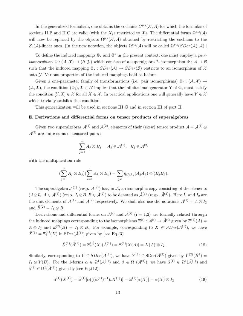
In the generalized formalism, one obtains the cochains Cp,s(X ,A) for which the formulas of

sections II B and II C are valid (with the Xjs restricted to X ). The differential forms Ωp,s(A)

will now be replaced by the objects Ωp,s(X ,A) obtained by restricting the cochains to the

Z0(A)-linear ones. [In the new notation, the objects Ωp,s(A) will be called Ωp,s(SDer(A),A).]

To define the induced mappings Φ∗ and Φ∗ in the present context, one must employ a pair-

isomorphism Φ : (A,X ) → (B,Y) which consists of a superalgebra *- isomorphism Φ : A → B

such that the induced mapping Φ∗ : SDer(A) → SDer(B) restricts to an isomorphism of X

onto Y. Various properties of the induced mappings hold as before.

Given a one-parameter family of transformations (i.e. pair isomorphisms) Φt : (A,X ) →

(A,X ), the condition (Φt)∗X ⊂ X implies that the infinitesimal generator Y of Φt must satisfy

the condition [Y,X] ∈ X for all X ∈ X . In practical applications one will generally have Y ∈ X

which trivially satisfies this condition.

This generalization will be used in sections III G and in section III of part II.

E. Derivations and differential forms on tensor products of superalgebras

Given two superalgebras A(1) and A(2), elements of their (skew) tensor product A = A(1)⊗

A(2) are finite sums of tensored pairs :

m∑

j=1

Aj ⊗ Bj Aj ∈ A(1), Bj ∈ A(2)

with the multiplication rule

(

m∑

j=1

Aj ⊗ Bj)(

n∑

k=1

Ak ⊗ Bk) =∑

j,k

ηBjAk(AjAk) ⊗ (BjBk).

The superalgebra A(1) (resp. A(2)) has, in A, an isomorphic copy consisting of the elements

(A⊗I2, A ∈ A(1)) (resp. I1⊗B,B ∈ A(2)) to be denoted as A(1) (resp. A(2)). Here I1 and I2 are

the unit elements of A(1) and A(2) respectively. We shall also use the notations A(1) = A ⊗ I2

and B(2) = I1 ⊗ B.

Derivations and differential forms on A(i) and A(i) (i = 1,2) are formally related through

the induced mappings corresponding to the isomorphisms Ξ(i) : A(i) → A(i) given by Ξ(1)(A) =

A ⊗ I2 and Ξ(2)(B) = I1 ⊗ B. For example, corresponding to X ∈ SDer(A(1)), we have

X(1) = Ξ(1)∗ (X) in SDer(A(1)) given by [see Eq.(3)]

X(1)(A(1)) = Ξ(1)∗ (X)(A(1)) = Ξ(1)[X(A)] = X(A) ⊗ I2. (18)

Similarly, corresponding to Y ∈ SDer(A(2)), we have Y (2) ∈ SDer(A(2)) given by Y (2)(B2) =

I1 ⊗ Y (B). For the 1-forms α ∈ Ω1(A(1)) and β ∈ Ω1(A(2)), we have α(1) ∈ Ω1(A(1)) and

β(2) ∈ Ω1(A(2)) given by [see Eq.(12)]

α(1)(X(1)) = Ξ(1)[α(((Ξ(1))−1)∗X(1))] = Ξ(1)[α(X)] = α(X) ⊗ I2 (19)

13

and β(2)(Y (2)) = I1 ⊗ β(Y ). Analogous formulas hold for the higher forms.

We can extend the action of the superderivations X(1) ∈ SDer(A(1)) and Y (2) ∈ SDer(A(2))

to A(2) and A(1) respectively by defining

X(1)(B(2)) = 0, Y (2)(A(1)) = 0 for all A ∈ A(1) and B ∈ A(2). (20)

Note that an X ∈ SDer(A) is determined completely by its action on the subalgebras A(1)

and A(2) :

X(A ⊗ B) = X(A(1)B(2)) = (XA(1))B(2) + ηXAA(1)X(B(2)).

With the extensions described above, we have available to us superderivations belonging to the

span of terms of the form [see Eq.(18)]

X = X(1) ⊗ I2 + I1 ⊗ X(2). (21)

Replacing I2 and I1 in Eq.(21) by elements of Z(A(2)) and Z(A(1)) respectively, we again obtain

superderivations of A. We, therefore, have the space of superderivations

[SDer(A(1)) ⊗ Z(A(2))] ⊕ [Z(A(1)) ⊗ SDer(A(2))]. (22)

This space, however, is generally only a Lie sub-superalgebra of SDer(A). For example, for

A(1) = Mm(C) and A(2) = Mn(C)(m,n > 1), recalling that all the derivations of these matrix

algebras are inner and that their centers consist of scalar multiples of the respective unit

matrices , we have the (complex) dimensions of SDer(A(1)), and SDer(A(2)) respectively, (m2−

1) and (n2−1) [so that the dimension of the space (22) is m2+n2−2 ] whereas that of SDer(A)

is (m2n2 − 1).

We shall need to employ (in section IV) a class of superderivations more general than (22).

To this end, it is instructive to obtain explicit representation(s) for a general derivation of the

matrix algebra A = Mm(C) ⊗ Mn(C). We have

[A ⊗ B,C ⊗ D]ir,js = AikBrtCkjDts − CikDrtAkjBts

which gives

[A ⊗ B,C ⊗ D]− = AC ⊗ BD − CA⊗ DB (23)

= [A,C]− ⊗1

2[B,D]+ +

1

2[A,C]+ ⊗ [B,D]−. (24)

This gives, in obvious notation,

DA⊗B ≡ [A ⊗ B, .]− = A.(.) ⊗ B.(.) − (.).A ⊗ (.).B (25)

= DA ⊗ JB + JA ⊗ DB (26)

where JB is the linear mapping on A(2) given by JB(D) = 12 [B,D]+ and a similar expression for

JA as a linear mapping on A(1). Eq.(25) shows that a derivation of the algebra A = A(1)⊗A(2)

14

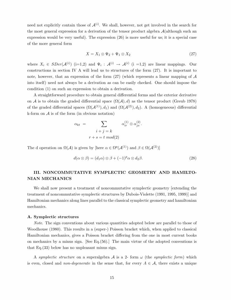
need not explicitly contain those of A(i). We shall, however, not get involved in the search for

the most general expression for a derivation of the tensor product algebra A(although such an

expression would be very useful). The expression (26) is more useful for us; it is a special case

of the more general form

X = X1 ⊗ Ψ2 + Ψ1 ⊗ X2 (27)

where Xi ∈ SDer(A(i)) (i=1,2) and Ψi : A(i) → A(i) (i =1,2) are linear mappings. Our

constructions in section IV A will lead us to structures of the form (27). It is important to

note, however, that an expression of the form (27) (which represents a linear mapping of A

into itself) need not always be a derivation as can be easily checked. One should impose the

condition (1) on such an expression to obtain a derivation.

A straightforward procedure to obtain general differential forms and the exterior derivative

on A is to obtain the graded differential space (Ω(A), d) as the tensor product (Greub 1978)

of the graded differential spaces (Ω(A(1)), d1) and (Ω(A(2)), d2). A (homogeneous) differential

k-form on A is of the form (in obvious notation)

αkt =∑

i + j = k

r + s = t mod(2)

α(1)ir ⊗ α

(2)js .

The d operation on Ω(A) is given by [here α ∈ Ωp(A(1)) and β ∈ Ω(A(2))]

d(α ⊗ β) = (d1α) ⊗ β + (−1)pα ⊗ d2β. (28)

III. NONCOMMUTATIVE SYMPLECTIC GEOMETRY AND HAMILTO-

NIAN MECHANICS

We shall now present a treatment of noncommutative symplectic geometry [extending the

treatment of noncommutative symplectic structures by Dubois-Violette (1991, 1995, 1999)] and

Hamiltonian mechanics along lines parallel to the classical symplectic geometry and hamiltonian

mechanics.

A. Symplectic structures

Note. The sign conventions about various quantities adopted below are parallel to those of

Woodhouse (1980). This results in a (super-) Poisson bracket which, when applied to classical

Hamiltonian mechanics, gives a Poisson bracket differing from the one in most current books

on mechanics by a minus sign. [See Eq.(56).] The main virtue of the adopted conventions is

that Eq.(33) below has no unpleasant minus sign.

A symplectic structure on a superalgebra A is a 2- form ω (the symplectic form) which

is even, closed and non-degenerate in the sense that, for every A ∈ A, there exists a unique

15

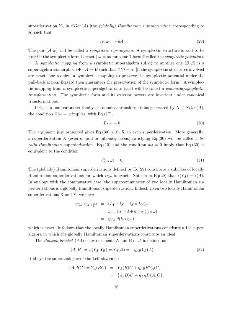
superderivation YA in SDer(A) [the (globally) Hamiltonian superderivation corresponding to

A] such that

iYAω = −dA. (29)

The pair (A, ω) will be called a symplectic superalgebra. A symplectic structure is said to be

exact if the symplectic form is exact ( ω = dθ for some 1-form θ called the symplectic potential).

A symplectic mapping from a symplectic superalgebra (A, α) to another one (B, β) is a

superalgebra isomorphism Φ : A → B such that Φ∗β = α. [If the symplectic structures involved

are exact, one requires a symplectic mapping to preserve the symplectic potential under the

pull-back action; Eq.(15) then guarantees the preservation of the symplectic form.] A symplec-

tic mapping from a symplectic superalgebra onto itself will be called a canonical/symplectic

transformation. The symplectic form and its exterior powers are invariant under canonical

transformations.

If Φt is a one-parameter family of canonical transformations generated by X ∈ SDer(A),

the condition Φ∗t ω = ω implies, with Eq.(17),

LXω = 0. (30)

The argument just presented gives Eq.(30) with X an even superderivation. More generally,

a superderivation X (even or odd or inhomogeneous) satisfying Eq.(30) will be called a lo-

cally Hamiltonian superderivation. Eq.(10) and the condition dω = 0 imply that Eq.(30) is

equivalent to the condition

d(iXω) = 0. (31)

The (globally) Hamiltonian superderivations defined by Eq(29) constitute a subclass of locally

Hamiltonian superderivations for which iXω is exact. Note from Eq(29) that ǫ(YA) = ǫ(A).

In analogy with the commutative case, the supercommutator of two locally Hamiltonian su-

perderivations is a globally Hamiltonian superderivation. Indeed, given two locally Hamiltonian

superderivations X and Y, we have

ηXω i[X,Y ]ω = (LY iX − iX LY )ω

= ηY ω (iY d + d iY )(iXω)

= ηY ω d(iY iXω)

which is exact. It follows that the locally Hamiltonian superderivations constitute a Lie super-

algebra in which the globally Hamiltonian superderivations constitute an ideal.

The Poisson bracket (PB) of two elements A and B of A is defined as

A,B = ω(YA, YB) = YA(B) = −ηABYB(A). (32)

It obeys the superanalogue of the Leibnitz rule :

A,BC = YA(BC) = YA(B)C + ηABBYA(C)

= A,BC + ηABBA,C.

16

As in the classical case, we have the relation

[YA, YB ] = YA,B. (33)

Eqn.(33) follows by using the equation for i[X,Y ]ω above with X = YA and Y = YB and

equations (32) and (29), remembering that Eq.(29) determines YA uniquely. The super-Jacobi

identity

0 =1

2(dω)(YA, YB , YC)

= A, B,C + (−1)ǫA(ǫB+ǫC)B, C,A

+(−1)ǫC(ǫA+ǫB)C, A,B (34)

is obtained by using Eq.(11) and noting that

YA[ω(YB, YC)] = A, B,C

ω([YA, YB], YC) = ω(YA,B, YC) = A,B, C.

Clearly, the pair (A, , ) is a Lie superalgebra. Eq.(33) shows that the linear mapping A 7→ YA

is a Lie-superalgebra homomorphism.

An element A of A can act, via YA, as the infinitesimal generator of a one-parameter family

of canonical transformations. The change in B ∈ A due to such an infinitesimal transformation

is

δB = ǫYA(B) = ǫA,B. (35)

In particular, if δB = ǫI (infinitesimal ‘translation’ in B), we have

A,B = I (36)

which is the noncommutative analogue of the classical PB relation p, q = 1. A pair (A,B) of

elements of A satisfying the condition (36) will be called a canonical pair.

B. Reality properties of the symplectic form and the Poisson bracket

For classical superdynamical systems, conventions about reality properties of the symplectic

form are based on the fact that the Lagrangian is a real, even object (Berezin and marinov

1977; Dass 1993). The matrix of the symplectic form is then real- antisymmetric in the ‘bosonic

sector’ and imaginary-symmetric in the ‘fermionic sector’ (which means anti-Hermitian in both

sectors). Keeping this in view, it appears appropriate to impose, in noncommutative Hamilto-

nian mechanics, the following reality condition on the symplectic form ω:

ω∗(X,Y ) = −ηXY ω(Y,X) for all X,Y ∈ SDer(A); (37)

but this means, by Eq.(7), that ω∗ = ω (i.e. ω is real) which is the most natural assumption

to make about ω. Eq.(37) is equivalent to the condition

ω(X∗, Y ∗) = −ηXY [ω(Y,X)]∗.

17

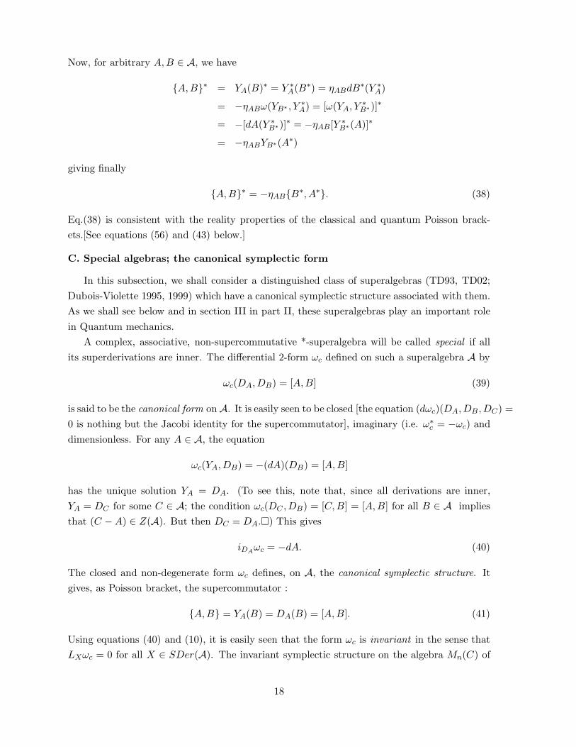
Now, for arbitrary A,B ∈ A, we have

A,B∗ = YA(B)∗ = Y ∗A(B∗) = ηABdB∗(Y ∗

A)

= −ηABω(YB∗ , Y ∗A) = [ω(YA, Y ∗

B∗)]∗

= −[dA(Y ∗B∗)]∗ = −ηAB[Y ∗

B∗(A)]∗

= −ηABYB∗(A∗)

giving finally

A,B∗ = −ηABB∗, A∗. (38)

Eq.(38) is consistent with the reality properties of the classical and quantum Poisson brack-

ets.[See equations (56) and (43) below.]

C. Special algebras; the canonical symplectic form

In this subsection, we shall consider a distinguished class of superalgebras (TD93, TD02;

Dubois-Violette 1995, 1999) which have a canonical symplectic structure associated with them.

As we shall see below and in section III in part II, these superalgebras play an important role

in Quantum mechanics.

A complex, associative, non-supercommutative *-superalgebra will be called special if all

its superderivations are inner. The differential 2-form ωc defined on such a superalgebra A by

ωc(DA,DB) = [A,B] (39)

is said to be the canonical form on A. It is easily seen to be closed [the equation (dωc)(DA,DB ,DC) =

0 is nothing but the Jacobi identity for the supercommutator], imaginary (i.e. ω∗c = −ωc) and

dimensionless. For any A ∈ A, the equation

ωc(YA,DB) = −(dA)(DB) = [A,B]

has the unique solution YA = DA. (To see this, note that, since all derivations are inner,

YA = DC for some C ∈ A; the condition ωc(DC ,DB) = [C,B] = [A,B] for all B ∈ A implies

that (C − A) ∈ Z(A). But then DC = DA.) This gives

iDAωc = −dA. (40)

The closed and non-degenerate form ωc defines, on A, the canonical symplectic structure. It

gives, as Poisson bracket, the supercommutator :

A,B = YA(B) = DA(B) = [A,B]. (41)

Using equations (40) and (10), it is easily seen that the form ωc is invariant in the sense that

LXωc = 0 for all X ∈ SDer(A). The invariant symplectic structure on the algebra Mn(C) of

18

complex n × n matrices obtained by Dubois-Violette and coworkers (1994) is a special case of

the canonical symplectic structure on special algebras described above.

If, on a special superalgebra A, instead of ωc, we take ω = b ωc as the symplectic form

(where b is a nonzero complex number), we have

YA = b−1DA, A,B = b−1[A,B]. (42)

The quantum Poisson bracket

A,BQ = (−i~)−1[A,B] (43)

is a special case of this with b = −i~. (Note that b must be imaginary to make ω real.) In

the case of the Schrodinger representation for a nonrelativistic spinless particle, the algebra A

generated by the position and momentum operators Xj, Pj (j= 1,2,3) defined on an invariant

domain in the Hilbert space H = L2(R3, dx) is special (Dubois-Violette 1995,1999); one has,

therefore, a canonical form ωc and the quantum symplectic structure on A given by the quantum

symplectic form

ωQ = −i~ωc (44)

which gives the PB (43).

We shall refer to a symplectic structure of the above sort with a general nonzero b as the

quantum symplectic structure with parameter b.

D. Noncommutative Hamiltonian mechanics

We shall now present the formalism of noncommutative Hamiltonian mechanics (NHM)

combining elements of noncommutative symplectic geometry and noncommutative probability

as mentioned earlier.

The system algebra and states

In NHM, one associates, with every physical system, a symplectic superalgebra (A, ω). Here

we shall treat the term ‘physical system’ informally as is traditionally done; some formalities

in this connection will be taken care of in section V in part II where the axioms are stated.

The even Hermitian elements of A represent observables of the system. The collection of all

observables in A will be denoted as O(A).

To take care of limit processes and continuity of mappings, we must employ topological

algebras. The choice of the admissible class of topological algebras must meet the following

reasonable requirements:

(i) It should be closed under the formation of (a) topological completions and (b) tensor prod-

ucts. [Both are nontrivial requirements (Dubin and Hennings 1990).]

(ii) It should include

19

(a) the Op∗-algebras (Horuzhy 1990) based on the pairs (H,D) where H is a separable Hilbert

space and D a dense linear subset of H. [Such an algebra is an algebra of operators which,

along with their adjoints, map D into itself. The *-operation on the algebra is defined as the

restriction of the Hilbert space adjoint on D. These are the algebras of operators (not neces-

sarily bounded) appearing in the traditional Hilbert space QM; for example, the (Heisenberg-

Schrodinger) operator algebra A in subsection C above belongs to this class.];

(b) Algebras of smooth functions on manifolds (to accommodate classical dynamics).

(iii) The GNS representations of the system algebra (in the non-supercommutative case) in-

duced by various states must have separable Hilbert spaces as the representation spaces.

The right choice appears to be the ⊗-(star-)algebras of Helemskii (1989) (i.e. locally convex

*-algebras which are complete and Hausdorff with a jointly continuous product) satisfying the

additional condition of being separable. [Note. The condition of separability may have to be

dropped in applications to quantum field theory.] Henceforth all (super-)algebras employed

will be assumed to belong to this class. For easy reference, unital *-algebras of this class will

be called NHM-admissible.

A state on a (unital) *-algebra A is a linear functional φ on A which is (i) positive [which

means φ(A∗A) ≥ 0 for all A ∈ A) and (ii) normalized [i.e. φ(I) = 1]. Given a state φ, the

quantity φ(A) for any observable A is real (this can be seen by considering, for example, the

quantityφ[(I +A)∗(I +A)]) and is to be interpreted as the expectation value of A in the state φ.

Following general usage in literature, we shall call observables of the form A∗A or sum of such

terms positive (strictly speaking, the term ‘non-negative’ would be more appropriate); states

assign non-negative expectation values to such observables. The family of all states on A will

be denoted as S(A). It is easily seen to be closed under convex combinations: given φi ∈ S(A)

, i = 1,..,n and pi ≥ 0 with p1 + .. + pn = 1, we have φ =∑n

i=1 piφi also in S(A). States which

cannot be expressed as nontrivial convex combinations of other states will be called pure states

and others mixed states or mixtures. The family of pure states of A will be denoted as S1(A).

The triple (A,S1(A), ω) will be referred to as a symplectic triple.

Expectation values of all even elements of A can be expressed in terms of those of the ob-

servables (by considering the breakup of such an element into its Hermitian and anti-Hermitian

part). This leaves out the odd elements of A. It appears reasonable to demand that the expec-

tation values φ(A) of all odd elements A ∈ A must vanish for all pure states (and, therefore,

for all states).

Denoting the algebraic dual of the superalgebra A by A∗, an automorphism Φ : A → A

induces the transpose mapping Φ : A∗ → A∗ such that

Φ(φ)(A) = φ(Φ(A)) or < Φ(φ), A > = < φ,Φ(A) > (45)

where the second alternative has employed the dual space pairing <,>. The mapping Φ (which

is easily seen to be linear and bijective) maps states (which form a subset of A∗) onto states.

To see this, note that

20

(i) Φ(φ)(A∗A) = φ(Φ(A∗A)) = φ(Φ(A)∗Φ(A)) ≥ 0;

(ii)[Φ(φ)](I) = φ(Φ(I)) = φ(I) = 1.

The linearity of Φ (as a mapping on A∗ ) ensures that it preserves convex combinations of

states. In particular, it maps pure states onto pure states. We have, therefore, a bijective

mapping Φ : S1(A) → S1(A).

When Φ is a canonical transformation, the condition Φ∗ω = ω gives, for X,Y ∈ SDer(A),

ω(X,Y ) = (Φ∗ω)(X,Y ) = Φ−1[ω(Φ∗X,Φ∗Y )]

which gives

Φ[ω(X,Y )] = ω(Φ∗X,Φ∗Y ). (46)

Taking expectation value of both sides of this equation in a state φ, we get

(Φφ)[ω(X,Y )] = φ[ω(Φ∗X,Φ∗Y )]. (47)

When Φ is an infinitesimal canonical transformation generated by G ∈ A, we have

Φ(φ)(A) = φ(Φ(A)) ≃ φ(A + ǫG,A).

Putting Φ(φ) = φ + δφ, we have

(δφ)(A) = ǫφ(G,A). (48)

Dynamics

Dynamics of the system is described in terms of the one-parameter family Φt of canonical

transformations generated by an observable H, called the Hamiltonian. (The parameter t

is supposed to be an evolution parameter which need not always be the conventional time.)

Writing Φt(A) = A(t) and recalling Eq.(35), we have the Hamilton’s equation of NHM :

dA(t)

dt= YH [A(t)] = H,A(t). (49)

The triple (A, ω,H) [or, more appropriately, the quadruple (A,S1(A), ω,H)] will be called an

NHM Hamiltonian system. It is the analogue of a classical Hamiltonian system (M,ωcl,Hcl)

[where (M, ωcl) is a symplectic manifold and Hcl, the classical Hamiltonian (a smooth real-

valued function on M); note that the specification of the symplectic manifold M serves to define

both observables and pure states in classical mechanics]. As far as the evolution is concerned,

the Hamiltonian is, as in the classical case, arbitrary up to the addition of a constant multiple of

the identity element. We shall assume that H is bounded below in the sense that its expectation

values in all pure states (hence in all states) are bounded below.

21

This is the analogue of the Heisenberg picture in traditional QM. An equivalent description,

the analogue of the Schrodinger picture, is obtained by transferring the time dependence to

states through the relation [see Eq.(45)]

< φ(t), A >=< φ,A(t) > (50)

where φ(t) = Φt(φ). The mapping Φt satisfies the condition (47) which [with Φ = Φt] may be

said to represent the canonicality of the evolution of states. With Φ = Φt and G = H, Eq.(48)

gives the Liouville equation of NHM:

dφ(t)

dt(A) = φ(t)(H,A) or

dφ(t)

dt(.) = φ(t)(H, .). (51)

Equivalent descriptions; Symmetries and conservation laws

By a ‘description’ of a system, we shall mean specification of its triple (A,S(A), ω). Two

descriptions are said to be equivalent if they are related through a pair of isomorphisms Φ1 :

A → A and Φ2 : S(A) → S(A) such that the symplectic form and the expectation values are

preserved :

Φ∗1ω = ω; Φ2(φ)[Φ1(A)] = φ(A) (52)

for all A ∈ A and φ ∈ S(A). The second equation above and Eq(45) imply that we must

have Φ2 = (Φ1)−1. Two equivalent descriptions are, therefore, related through a canonical

transformation on A and the corresponding inverse transpose transformation on the states. An

infinitesimal transformation of this type generated by G ∈ A takes the form

δA = ǫG,A, (δφ)(A) = −ǫφ(G,A) (53)

for all A ∈ A and φ ∈ S(A).

These transformations may be called symmetries of the formalism; they are the analogues

of simultaneous unitary transformations on operators and state vectors in a Hilbert space

preserving expectation values of operators. Symmetries of dynamics are the subclass of these

which leave the Hamiltonian invariant:

Φ1(H) = H. (54)

For an infinitesimal transformation generated by G ∈ A, this equation gives

G,H = 0. (55)

It now follows from the Hamilton’s equation (49) that (in the ‘Heisenberg picture’ evolution) G

is a constant of motion. This is the situation familiar from classical and quantum mechanics:

generators of symmetries of the Hamiltonian are conserved quantities and vice-versa.

Note. Noting that a symmetry operation is uniquely defined by any one of the two mappings

Φ1 and Φ2, we can be flexible in the implementation of symmetry operations. It is often

22

useful to implement them such that the symmetry operations act, in a single implementation,

either on states or on observables, and the two actions are related as the Heisenberg and

Schrodinger picture evolutions above [see equations (50) and (45)]; we shall refer to this type

of implementation as unimodal. In such an implementation, the second equation in (53) will

not have a minus sign on the right.

For future reference, we define equivalence of NHM Hamiltonian systems. Two NHM Hamil-

tonian systems

(A,S1(A), ω,H) and (A′,S1(A′), ω′,H ′)

are said to be equivalent if they are related through a pair Φ = (Φ1,Φ2) of bijective mappings

such that Φ1 : (A, ω) → (A′, ω′) is a symplectic mapping connecting the Hamiltonians [i.e.

Φ∗1ω

′ = ω and Φ1(H) = H ′] and Φ2 : S1(A) → S1(A′) such that < Φ2(φ),Φ1(A) >=< φ,A > .

Classical Hamiltonian mechanics and traditional Hilbert space QM as subdisci-

plines of NHM

A classical hamiltonian system (M,ωcl,Hcl) is a special case of an NHM Hamiltonian system

(A, ω,H) with A = Acl ≡ C∞(M), ω = ωcl ≡∑

dpj ∧ dqj and H = Hcl; the NHM PBs are

now the classical PBs

f, gcl =

n∑

j=1

(∂f

∂pj

∂g

∂qj−

∂f

∂qj

∂g

∂pj

). (56)

Eq.(49) now becomes the classical Hamilton’s equation. Representing states by probability

densities in phase space, Eq.(51) goes over, in appropriate cases (for M = R2n, for example,

after the obvious partial integrations) to the classical Liouville equation for the density function.

To see the traditional Hilbert space QM as a subdiscipline of NHM, it is useful to introduce

the concept of a quantum triple (H,D,A) where H is a complex separable Hilbert space, D a

dense linear subset of H and A an Op-∗-algebra of operators based on (H,D). When A is special

in the sense of section III C (this is the case for the Schrodinger dynamics of a finite number

of nonrelativistic particles and is trivially so for spin dynamics), choosing an appropriate self

adjoint element H of A as the Hamiltonian operator, we have a quantum hamiltonian system

(A, ωQ,H) [with ωQ as in Eq.(44)] as a special case of an NHM Hamiltonian system. With

the quantum PBs of Eq.(43), Eq.(49) goes over to the Heisenberg equation. The states are

represented by density operators ρ satisfying the condition |Tr(ρA)| < ∞ for all observables A

in A; Eq.(51) then goes over to the von Neumann equation

dρ(t)

dt= (−i~)−1[ρ(t),H]. (57)

E. Symplectic actions of Lie groups

The study of symplectic actions of Lie groups in NHM proceeds generally parallel to the

classical case (Sudarshan and Mukunda 1974; Arnold 1978; Guillemin and Sternberg 1984;

23

Woodhouse 1980) and promises to be quite rich and rewarding. Here we shall present the

essential developments mainly to provide background material for the following sections.

Let G be a connected Lie group with Lie algebra G. Elements of G, G and G∗ (the dual space

of G) will be denoted, respectively, as g,h,.., ξ, η, .. and λ, µ, ... The pairing between G∗ and G

will be denoted as < ., . >. Choosing a basis ξa; a = 1, .., r in G, we have the commutation

relations [ξa, ξb] = Ccabξc. The dual basis in G∗ is denoted as λa (so that < λa, ξb >= δa

b ).

The action of G on G (adjoint representation) will be denoted as Adg : G → G and that on

G∗ (the coadjoint representation) by Cadg : G∗ → G∗; the two are related as < Cadgλ, ξ >=<

λ,Adg−1ξ > . With the bases chosen as above, the matrices in the two representations are

related as (Cadg)ab = (Adg−1)ba.

Recalling the mappings Φ1 and Φ2 of the previous subsection, a symplectic action of of G

on a symplectic superalgebra (A, ω) is given by the assignment, to each g ∈ G, a symplectic

mapping (canonical transformation) Φ1(g) : A → A which is a group action [which means that

Φ1(g)Φ1(h) = Φ1(gh) and Φ1(e) = idA in obvious notation]. The action on the states is given

by the mappings Φ2(g) = [Φ1(g)]−1.

A one-parameter subgroup g(t) of G generated by ξ ∈ G induces a locally Hamiltonian

derivation Zξ ∈ SDer(A) as the generator of the one-parameter family Φ1(g(t)−1) of canonical

transformations of A: For small t

Φ1(g(t)−1)(A) ≃ A + tZξ(A).

[Note. We employed Φ1(g(t)−1) (and not Φ1(g(t))) for defining Zξ above because the for-

mer correspond to a right action of G on A.] The correspondence ξ → Zξ is a Lie algebra

homomorphism :

Z[ξ,η] = [Zξ, Zη]. (58)

[A proof of (58), whose steps are parallel to those for Lie group actions on manifolds, was given

in TD08 (it is an instructive application of the mathematical techniques of section II); we shall

skip the details here.]

The G-action is said to be hamiltonian if the derivations Zξ are Hamiltonian, i.e. for

each ξ ∈ G, Zξ = Yhξfor some hξ ∈ A (called the hamiltonian corresponding to ξ). These

hamiltonians are arbitrary up to addition of multiples of the unit element. This arbitrariness

can be somewhat reduced by insisting that hξ be linear in ξ.(This can be achieved by first

defining the hamiltonians for the members of a basis in G and then for general elements as

appropriate linear combinations of these.) We shall always assume this linearity.

A hamiltonian G-action satisfying the additional condition

hξ , hη = h[ξ,η] for all ξ, η ∈ G (59)

is called a Poisson action. The hamiltonians of a Poisson action have the following equivariance

property :

Φ1(g)(hξ) = hAdg(ξ). (60)

24

Since G is connected, it is adequate to verify this relation for infinitesimal group actions.

Denoting by g(t) the one-parameter group generated by η ∈ G, we have, for small t,

Φ1(g(t))(hξ) ≃ hξ + thη , hξ = hξ + th[η,ξ] = hξ+t[η,ξ] ≃ hAdg(t)ξ

completing the verification.

A Poisson action is not always admissible. The obstruction to such an action is determined

by the objects

α(ξ, η) = hξ, hη − h[ξ,η] (61)

which are easily seen to have vanishing Hamiltonian derivations :

Yα(ξ,η) = [Yhξ, Yhη ] − Yh[ξ,η]

= [Zξ, Zη] − Z[ξ,η] = 0

and hence vanishing Poisson brackets with all elements of A. [This last condition defines the

so-called neutral elements (Sudarshan and Mukunda 1974) of the Lie algebra(A, , ). They

clearly form a complex vector space which will be denoted as N .] We also have

α([ξ, η], ζ) + α([η, ζ], ξ) + α([ζ, ξ], η) = 0.

The derivation (Woodhouse 1980) of this result in classical mechanics employs only the standard

properties of PBs and remains valid in NHM. Comparing this equation with Eq.(6), we see that

α(., .) ∈ Z20 (G,N ). A redefinition of the hamiltonians hξ → h′

ξ = hξ + kξI (where the scalars

kξ are linear in ξ) changes α by a coboundary term:

α′(ξ, η) = α(ξ, η) − k[ξ,η]I

showing that the obstruction is characterized by a cohomology class of G [i.e. an element of

H20 (G,N )]. A necessary and sufficient condition for the admissibility of Poisson action of G on

A is that it should be possible to transform away all the obstruction 2-cocycles by redefining

the hamiltonians, or, equivalently, H20 (G,N ) = 0.

We restrict ourselves to the special case, relevant for application in section II in part II, in

which the cocycles α are multiples of the unit element :

α(ξ, η) = α(ξ, η)I; (62)

here the quantities α(ξ, η) must be real numbers because the set of observables is closed under

Poisson brackets. This implies N = R, the set of real numbers. In this case, the relevant

cohomology group H20 (G, R) is a real finite dimensional vector space; we shall take it to be Rm.

In this case, as in classical symplectic mechanics (Sudarshan and Mukunda 1974; Carinena

and Santander 1975; Alonso 1979), Hamiltonian group actions (more generally, Lie algebra

actions) with nontrivial neutral elements can be treated as Poisson actions of a (Lie group with

a) larger Lie algebra G obtained as follows: Let ηr(., .)(r = 1, ..,m) be a set of representatives

25

in Z20 (G, R) of a basis in H2

0 (G, R). We add extra generators Mr to the basis ξa of G and

take the commutation relations of the larger Lie algebra G as

[ξa, ξb] = Ccabξc +

m∑

r=1

ηr(ξa, ξb)Mr; [ξa,Mr] = 0 = [Mr,Ms]. (63)

The simply connected Lie group G with the Lie algebra G is called the projective group of

G(called ‘projective covering group’ of G by Carinena and Santander; we follow the terminology

of Alonso 1979); it is generally a central extension of the universal covering group G of G.

The hamiltonian action of G with the cocycle α now becomes a Poisson action of G with

the Poisson bracket relations (writing hMr = hr)

ha, hb = Ccabhc +

m∑

r=1

ηr(ξa, ξb)hr; ha, hr = 0 = hr, hs. (64)

F. The momentum map.

In classical mechanics, given a Poisson action of a connected Lie group G on a symplectic

manifold (M,ωcl) [with hamiltonians/comoments h(cl)ξ ∈ C∞(M)], a useful construction is the

so-called momentum map(Souriau 1997; Arnold 1978; Guillemin and Sternberg 1984) P : M →

G∗ given by

< P (x), ξ > = h(cl)ξ (x) ∀x ∈ M and ξ ∈ G. (65)

This map relates the symplectic action Φg of G on M (Φg : M → M,Φ∗gωcl = ωcl ∀g ∈ G) and

the transposed adjoint action on G∗ through the equivariance property

P (Φg(x)) = Ad∗g(P (x)) ∀x ∈ M and g ∈ G. (66)

Noting that points of M are pure states of the algebra Acl = C∞(M), the map P may be

considered as the restriction to M of the dual/transpose h(cl) : A∗cl → G∗ of the linear map

h(cl) : G → Acl [given by h(cl)(ξ) = h(cl)ξ ]:

< h(cl)(u), ξ >=< u, h(cl)(ξ) > ∀ u ∈ A∗cl and ξ ∈ G.

The analogue of M in NHM is S1 = S1(A). Defining h : G → A by h(ξ) = hξ, the analogue of

the momentum map in NHM is the mapping h : S1 → G∗ (considered as the restriction to S1

of the mapping h : A∗ → G∗) given by

< h(φ), ξ >=< φ, h(ξ) >=< φ, hξ > . (67)

Now

< h(Φ2(g)φ), ξ > = < Φ2(g)φ, hξ >=< φ,Φ1(g−1)(hξ) >=< φ, hAd

g−1 (ξ) >

= < φ, h(Adg−1(ξ)) >=< Cadg(h(φ)), ξ >

26

giving finally

h(Φ2(g)φ) = Cadg(h(φ)) (68)

which is the noncommutative analogue of Eq.(66). [Note. In Eq.(68),the co-adjoint (and not

the transposed adjoint) action appears on the right because Φ2(g) is inverse transpose (and not

transpose) of Φ1(g). With this understanding, (66) is obviously a special case of (68).]

G. Generalized symplectic structures and Hamiltonian systems

The generalization of the DVNCG scheme introduced in section II D can be employed to

obtain the corresponding generalization of the NHM formalism. One picks up a distinguished

Lie sub-superalgebra X of SDer(A) and restricts the superderivations of A in all definitions

and constructions to those in X . Thus, a symplectic superalgebra (A, ω) is now replaced by

a generalized symplectic superalgebra (A,X , ω) and a symplectic mappings Φ : (A,X , α) →

(B,Y, β) is restricted to a superalgebra-isomorphism Φ : A → B such that Φ∗ : X → Y is a

Lie-superalgebra- isomorphism and Φ∗β = α. An NHM Hamiltonian system (A,S1(A), ω,H)

is now replace by a generalized NHM Hamiltonian sytem (A,S1(A),X , ω,H). In section III of

part II, we shall employ the pairs (A, X ) with X= ISDer(A) to define quantum symplectic

structure on superalgebras admitting outer as well as inner superderivations.

H. Augmented symplectics including time; the noncommutative analogue of Poincare-

Cartan form

We shall now augment the kinematic framework of NHM by including time and obtain

the non-commutative analogues of the Poincare-Cartan form and the symplectic version of

Noether’s theorem (Souriau 1997).

For a system S with associated symplectic superalgebra (A, ω) we construct the extended

system algebra Ae = C∞(R) ⊗ A (where the real line R is the carrier space of the ‘time’ t)

whose elements are finite sums∑

i fi ⊗ Ai (with fi ∈ C∞(R) ≡ A0) which may be written

as∑

i fiAi. This algebra is the analogue of the algebra of functions on the evolution space of

Souriau (the Cartesian product of the time axis and the phase space — often referred to as the

phase bundle).The superscript e in Ae, may, therefore, also be taken to refer to ‘evolution’.

Derivations on A0 are of the form g(t) ddt and one-forms of the form h(t)dt where g and h

are smooth functions; there are no nonzero higher order forms. We have, of course, dt( ddt ) = 1.

A (super-)derivation D1 on A0 and D2 on A extend trivially to (super-)derivations on Ae

as D1 ⊗ idA and idA0 ⊗D2 respectively; these trivial extensions may be informally denoted as

D1 and D2. With f ⊗A written as fA, we can write D1(fA) = (D1f)A and D2(fA) = f(D2A).

The mapping Ξ : A → Ae given by Ξ(A) = 1⊗A(= A) is an isomorphism of the algebra A

onto the subalgebra A ≡ 1 ⊗A of Ae and can be employed to pull back the differential forms

on A to those on A. We write, for a p-form α on A, (Ξ−1)∗(α) = α and extend this form on

A to one on Ae by defining α( ddt , ...) = 0. We shall generally skip the tilde. Similarly, we may

extend the one-form dt on A0 to one on Ae by defining (dt)(X) =0 for all X ∈ SDer(A).

27

The symplectic structure ω on A induces, on Ae, a generalized symplectic structure (of

the type introduced in subsection G above) with the distinguished Lie sub-superalgebra X

of SDer(Ae) taken to be the one consisting of the objects idA0 ⊗ D;D ∈ SDer(A) which

constitute a Lie sub-superalgebra of SDer(Ae) isomorphic to SDer(A), thus giving a general-

ized symplectic superalgebra (Ae,X , ω). The corresponding PBs on Ae are trivial extensions

of those on A obtained by treating the ‘time’ t as an external parameter; this amounts to

extending the C-linearity of PBs on A to what is essentially A0-linearity :

fA + gB, hCAe = fhA,CA + ghB,CA

where, for clarity, we have put subscripts on the PBs to indicate the underlying superalgebras.

We shall often drop these subscripts; the underlying (super-)algebra will be clear from the

context.

To describe dynamics in Ae, we extend the one-parameter family Φt of canonical transforma-

tions on A generated by a Hamiltonian H ∈ A to a one-parameter family Φet of transformations

on Ae (which are ‘canonical’ in a certain sense, as we shall see below) given by

Φet(fA) ≡ (fA)(t) = f(t)A(t) ≡ (Φ

(0)t f)Φt(A)

where Φ(0)t is the one-parameter group of translations on A0 generated by the derivation d

dt .

An infinitesimal transformation under the evolution Φet is given by

δ(fA)(t) ≡ (fA)(t + δt) − (fA)(t)

= [df

dtA + fH,AA]δt ≡ YH(fA)δt

where

YH =∂

∂t+ YH . (69)

Here ∂∂t is the derivation on Ae corresponding to the derivation d

dt on A0 and

YH = H, .Ae . (70)

Note that

(i) dt(YH) = 1;

(ii) the right hand side of Eq.(70) remains well defined if H ∈ Ae (‘time dependent’ Hamil-

tonian). Henceforth, in various formulas in this subsection, H will be understood to be an

element of Ae.

The obvious generalization of the NHM Hamilton’s equation (49) to Ae is the equation

dF (t)

dt= YHF (t) =

∂F (t)

∂t+ H(t), F (t). (71)

We next consider an object in Ae which contains complete information about the symplectic

structure and dynamics [i.e. about ω and H (up to an additive constant multiple of I)] and is

canonically determined by these objects. It is the 2-form

Ω = ω + dt ∧ dH (72)

28

which is ‘obviously’ closed. [To have a formal proof, apply Eq.(28) with Ω = 1⊗ω+d1t⊗d2H.]

If the symplectic structure on A is exact (with ω = dθ), we have (‘obviously’) Ω = dΘ where

Θ = θ − Hdt (73)

is the NHM avatar of the Poincare-Cartan form in classical mechanics. [Again, for a formal

derivation, use Eq.(28) with Θ = 1 ⊗ θ − dt ⊗ H.]

The closed form Ω is generally not non-degenerate. It defines what may be called a presym-

plectic structure (Souriau 1997) on Ae. In fact, we have here the noncommutative analogue of

a special type of presymplectic structure called contact structure (Abraham and Marsden 1978;

Berndt 2001); it may be called the Poincare- Cartan contact structure. We shall, however, not

attempt a formal development of noncommutative contact structures here.

A symplectic action of a Lie group G on the presymplectic space (Ae,Ω) is the assignment,

to every g ∈ G, an automorphism Φ(g) of the superalgebra Ae having the usual group action

properties and such that Φ(g)∗Ω = Ω. This implies, as in section III E, that, to every element

ξ of the Lie algebra G of G, corresponds a derivation Zξ such that LZξΩ = 0 which, in view of

the condition dΩ = 0, is equivalent to the condition

d(iZξΩ) = 0. (74)

We shall now verify that the one-parameter family Φ(e)t of transformations on Ae is sym-

plectic/canonical. For this, it is adequate to verify that Eq.(74) holds with Zξ = YH . We have,

in fact, the stronger relation

iYHΩ = 0. (75)

Indeed

iYHΩ = i∂/∂tΩ + iYH

Ω

= i∂/∂t(dt ∧ dH) + iYHω + iYH

(dt ∧ dH)

= dH − dH − iYH(dH)dt

= [iYH(iYH

ω)]dt = 0.

The equation in note (i) above and Eq.(75) are analogous to the properties of the ‘char-

acteristic vector field’ of a contact structure. The derivation YH may, therefore, be called the

characteristic derivation of the Poincare-Cartan contact structure.

A symplectic G-action (in the present context) is said to be hamiltonian if the 1-forms iZξΩ

are exact, i.e. to each ξ ∈ G, corresponds a ‘hamiltonian’ hξ ∈ Ae (unique up to an additive

constant multiple of the unit element) such that

iZξΩ = −dhξ . (76)

29

These ‘hamiltonians’ (Noether invariants) are constants of motion :

dhξ(t)

dt= YH(hξ(t)) = (dhξ)(YH)(t)

= −(iZξΩ)(YH)(t) = 0 (77)

where, in the last step, Eq.(75) has been used. This is the NHM analogue of the symplectic

version of Noether’s theorem. Some concrete examples of Noether invariants will be given in

section II F in part II.

IV. COUPLED SYSTEMS IN NONCOMMUTATIVE HAMILTONIAN MECHAN-

ICS

We shall now consider the interaction of two systems S1 and S2 described individually as the

NHM Hamiltonian systems (A(i), ω(i),H(i)) (i=1,2) and treat the coupled system S1 + S2 also

as an NHM Hamiltonian system. To facilitate this, we must obtain the relevant mathematical

objects for the coupled system.

A. The symplectic form and Poisson bracket on the tensor product of two super-

algebras

We shall freely use the notations and constructions in section II E.

Given the symplectic forms ω(i) on A(i) [with PBs , i(i=1,2)] we shall construct the ‘canon-

ically induced’ symplectic form ω on A satisfying the following conditions :

(a) It should not depend on anything other than the objects ω(i) and I(i) (i=1,2) [the ‘natural-

ity’/‘canonicality’ assumption for ω. (Note that the unit elements are the only distinguished

elements of the algebras being considered)].

(b) The restrictions of ω to A(1) and A(2) be, respectively, ω(1) ⊗ I2 and I1 ⊗ ω(2).

This determines ω uniquely :

ω = ω(1) ⊗ I2 + I1 ⊗ ω(2). (78)

To verify that it is a symplectic form, we must show that it is (i) closed and (ii) nondegenerate.

Eq.(28) gives

dω = (d1ω(1)) ⊗ I2 + ω(1) ⊗ d2(I2) + d1(I1) ⊗ ω(2) + I1 ⊗ d2ω

(2) = 0

showing that ω is closed. To show the nondegeneracy of ω, it is necessary and sufficient to

show that, given A⊗B ∈ A, there exists a unique superderivation Y = YA⊗B in SDer(A) such

that

iY ω = −d(A ⊗ B) = −(d1A) ⊗ B − A ⊗ d2B

= iY

(1)A

ω(1) ⊗ B + A ⊗ iY

(2)B

ω(2). (79)

30

where Y(1)A and Y

(2)B are the Hamiltonian superderivations associated with A ∈ A(1) and B ∈

A(2). The structure of Eq.(79) suggests that Y must be of the form [see Eq.(27)]

Y = Y(1)A ⊗ Ψ

(2)B + Ψ

(1)A ⊗ Y

(2)B (80)

where the linear mappings Ψ(1)A and Ψ

(2)B satisfy the conditions Ψ

(1)A (I1) = A and Ψ

(2)B (I2) = B.

Recalling the discussion after Eq.(27) and Eq.(1) [and denoting the multiplication operators in

A(1),A(2) and A by µ1, µ2 and µ respectively], the (necessary and sufficient) condition for Y to

be a superderivation may be written as

Y µ(C ⊗ D) − ηY,C⊗D µ(C ⊗ D) Y = µ(Y (C ⊗ D)). (81)

Noting that µ(C ⊗ D) = µ1(C) ⊗ µ2(D) (the skew tensor product causes no problems here),

Eq.(81) with Y of Eq.(80) gives

ηBC[Y(1)A µ1(C)] ⊗ [Ψ

(2)B µ2(D)] + [Ψ

(1)A µ1(C)] ⊗ Y

(2)B µ2(D)]

−(−1)ǫ[µ1(C) Y(1)A ] ⊗ [µ2(D) Ψ

(2)B ] + [µ1(C) Ψ

(1)A ] ⊗ [µ2(D) Y

(2)B ]

= ηBC [µ1(A,C1) ⊗ µ2(Ψ(2)B (D)) + µ1(Ψ

(1)A (C)) ⊗ µ2(B,D2)] (82)

where ǫ ≡ ǫAǫC +ǫBǫD+ǫBǫC and we have used the relations Y(1)A (C) = A,C1 and Y

(2)B (D) =

B,D2.

The objects Y(1)A and Y

(2)B , being superderivations, satisfy relations of the form (1) :

Y(1)A µ1(C) − ηACµ1(C) Y

(1)A = µ1(Y

(1)A (C)) = µ1(A,C1)

Y(2)B µ2(D) − ηBDµ2(D) Y

(2)B = µ2(B,D2). (83)

Putting D = I2 in Eq.(82), we have [noting that µ2(D) = µ2(I2) = idA(2) , and B, I22 =

Y(2)B (I2) = 0]

[Y(1)A µ1(C)] ⊗ Ψ

(2)B + [Ψ

(1)A µ1(C)] ⊗ Y

(2)B

−ηAC[µ1(C) Y(1)A ] ⊗ Ψ

(2)B + [µ1(C) Ψ

(1)A ] ⊗ Y

(2)B

= µ1(A,C1) ⊗ µ2(B) (84)

which, along with equations (83), gives

µ1(A,C1) ⊗ [Ψ(2)B − µ2(B)] =

−[Ψ(1)A µ1(C) − ηACµ1(C) Ψ

(1)A ] ⊗ Y

(2)B . (85)

Similarly, putting C = I1 in Eq.(82), we get

[Ψ(1)A − µ1(A)] ⊗ µ2(B,D2) =

−Y(1)A ⊗ [Ψ

(2)B µ2(D) − ηBDµ2(D) Ψ

(2)B ]. (86)

Now, equations (86) and (85) give the relations

Ψ(1)A − µ1(A) = λ1Y

(1)A (87)

31

Ψ(2)B µ2(D) − ηBD µ2(D) Ψ

(2)B = −λ1 µ2(B,D2) (88)

Ψ(2)B − µ2(B) = λ2Y

(2)B (89)

Ψ(1)A µ1(C) − ηAC µ1(C) Ψ

(1)A = −λ2 µ1(A,C1) (90)

where λ1 and λ2 are complex numbers.

Equations (80), (87) and (89) now give

Y = Y(1)A ⊗ [µ2(B) + λ2Y

(2)B ] + [µ1(A) + λ1Y

(1)A ] ⊗ Y

(2)B

= Y(1)A ⊗ µ2(B) + µ1(A) ⊗ Y

(2)B + (λ1 + λ2)Y

(1)A ⊗ Y

(2)B . (91)

Note that only the combination (λ1 + λ2) ≡ λ appears in Eq.(91). To have a unique Y, we

must obtain an equation fixing λ in terms of given quantities.

Substituting for Ψ(1)A and Ψ

(2)B from equations (87) and (89) into equations (88) and (90)

and using equations (83), we obtain the equations

λµ1(A,C1) = −µ1([A,C]) for all A,C ∈ A(1) (92)

λµ2(B,D2) = −µ2([B,D]) for all B,D ∈ A(2). (93)

We have not one but two equations of the type we have been looking for. This is a signal

for the emergence of nontrivial conditions (for the desired symplectic structure on the tensor

product superalgebra to exist).

Let us consider the equations (92,93) for the various possible situations (corresponding to

whether or not one or both the superalgebras are super-commutative) :

(i) Let A(1) be supercommutative. Assuming that the PB , 1 is nontrivial, Eq.(92) implies

that λ = 0. Eq.(93) then implies that A(2) must also be super-commutative. It follows that

(a) when both the superalgebras A(1) and A(2) are super-commutative, the unique Y is given

by Eq.(91) with λ = 0;

(b) when one of them is supercommutative and the other is not, the ω of Eq.(78) does not

define a symplectic structure on A; hence a ‘canonically induced’ symplectic structure does not

exist on the tensor product of a super-commutative and a non-supercommutative superalgebra.

(ii) Let the superalgebra A(1) be non-supercommutative. Eq.(92) then implies that λ 6= 0,

which, along with Eq.(93) implies that the superalgebra A(2) is also non-supercommutative

[which is also expected from (b) above]. These equations now give

A,C1 = −λ−1[A,C], B,D2 = −λ−1[B,D] (94)

which shows that, when both the superalgebras are non-supercommutative, a ‘canonically in-

duced’ symplectic structure on their (skew) tensor product exists if and only if each superalgebra

has a quantum symplectic structure with the same parameter (−λ), i.e.

ω(1) = −λω(1)c , ω(2) = −λω(2)

c (95)

32

where ω(i)c (i=1,2) are the canonical symplectic forms on the two superalgebras. The traditional

quantum symplectic structure is obtained with λ = i~ [see Eq.(44)].

Note. The two forms ω(i)(i=1,2) of Eq.(95) represent genuine symplectic structures only if the

superalgebras A(i) (i=1,2) have only inner superderivations (see section III C). In general, we

have generalized symplectic superalgebras (A(i),X (i), ω(i)) (i=1,2) where X (i) = ISDer(A(i)).

In all the permitted cases, the PB on the superalgebra A = A(1) ⊗A(2) is given by

A ⊗ B,C ⊗ D = YA⊗B(C ⊗ D) = ηBC [A,C1 ⊗ BD + AC ⊗ B,D2

+λA,C1 ⊗ B,D2] (96)

where the parameter λ vanishes in the super-commutative case; in the non-supercommutative

case, it is the universal parameter appearing in the symplectic forms (95).

Noting that, in the non-supercommutative case,

λA,C1 ⊗ B,D2 = −[A,C] ⊗ B,D2 = −A,C1 ⊗ [B,D]

= −1

2[A,C] ⊗ B,D2 −

1

2A,C1 ⊗ [B,D],

the PB of Eq.(96) can be written in the more symmetric form

A ⊗ B,C ⊗ D

= ηBC [A,C1 ⊗BD+ηBDDB

2 + AC+ηACCA2 × B,D2].

(97)

Note. The non-super version of Eq.(97) was [wrongly, not realizing that Y of Eq.(80) is not

always a (super-)derivation] put forward by the author as the PB for a tensor product of

algebras in the general case [in arXiv : quant-ph/0612224, henceforth referred to as TD06].

M.J.W. Hall pointed out to the author (private communication) that it does not satisfy Jacobi

identity in some cases, as shown, for example, in (Caro and Salcedo, 1999). Revised calculations

by the author then led to the results presented above.

B. Dynamics of coupled systems

Given the individual systems S1 and S2 as the NHM Hamiltonian systems (A(i), ω(i),H(i)) (i

= 1,2) where the two superalgebras are either both supercommutative or both non-supercommutative,

the coupled system (S1+S2) is an NHM Hamiltonian system with the system algebra and sym-

plectic form as discussed above and the Hamiltonian H given by

H = H(1) ⊗ I2 + I1 ⊗ H(2) + Hint (98)

where the interaction Hamiltonian is generally of the form

Hint =n∑

i=1

Fi ⊗ Gi.

33

The evolution (in the Heisenberg type picture) of a typical obsevable A(t) ⊗ B(t) is governed

by the supmech Hamilton’s equation

d

dt[A(t) ⊗ B(t)] = H,A(t) ⊗ B(t)

= H(1), A(t)1 ⊗ B(t) + A(t) ⊗ H(2), B(t)2

+Hint, A(t) ⊗ B(t). (99)

The last Poisson bracket in this equation can be evaluated using Eq.(96) or (97). In the

Schrodinger type picture, the time evolution of states of the coupled system is given by the

NHM Liouville equation (51) with the Hamiltonian of Eq.(98). In favorable situations, the NHM

Heisenberg or Liouville equations may be written for finite time intervals by using appropriate

exponentiations of operators.

The main lesson from this section is that all systems in nature whose interaction with other

systems can be talked about must belong to one of the two ‘worlds’ : the ‘commutative world’

in which all system superalgebras are super-commutative and the ‘noncommutative world’ in

which all system superalgebras are non-supercommutative with a universal quantum symplectic

structure. In view of the familiar inadequacy of the commutative world, the ‘real’ world must

clearly be the noncommutative (hence quantum) world; its systems will be called quantum

systems. (This is formalized as axiom A7 in section V in part II.) The classical systems

with commutative system algebras and traditional symplectic structures will appear only in

the appropriately defined classical limit (or, more generally, in the classical approximation) of

quantum systems.

Concluding remarks and acknowledgements will appear in part II.

REFERENCES

Alonso, L.M. J. Math. Phys. 20, 219 (1979).

Arnold, V.I. :“Mathematical Methods of Classical Mechanics”, Springer-Verlag, New York (1978).

Bell, J. : “Speakable and Unspeakable in Quantum Mechanics”, Cambridge University Press (1988).

Berezin, F.A., Marinov, M.S.,Ann. Phys. 104, 336 (1977).

Bohm,D., Hiley, B.J. :“The Undivided Universe: An Ontological Interpretation of Quantum Theory”, Rout-

ledge, Chapman and Hall, London (1993).

Born, M., Heisenberg, W., Jordan, P.,Zs. f. Phys. 35, 557 (1926).

Born M., Jordan, P.,Zs. f. Phys. 34, 858 (1925).

Bratteli, O., Robinson, D.W. : “Operator algebras and quantum statistical mechanics I. C∗

− and W∗-algebras,

symmetry groups, decomposition of states”, Springer, New York (1979; II. “Equilibrium States; Models

in Quantum Statistical Mechanics”, ibid (1981).

Busch, P., Grabowski, M., Lahti, P.J. :“Operational Quantum Physics”, Springer-Verlag, Berlin (1995).

Carinena, J.F., Santander, M.,J. Math. Phys. 16, 1416 (1975).

Caro,J., Salcedo, L.L. :“Impediments to mixing classical and quantum dynamics”, Phys. Rev. A60, 842 (1999);

arXiv : quant-ph/9812046 v2 (April, 1999).

34

Cartan, H., Eilenberg, S. : “Homological Algebra”, Princeton University Press (1956).

Connes, A. :“Noncommutative geometry”, Academic Press, New York (1994).

Dass T. :“Symmetries, gauge fields, strings and fundamental interactions”, vol. I: “Mathematical techniques

in gauge and string theories”, Wiley Eastern Limited, New Delhi (1993).

Dirac P.A.M., Proc. Roy. Soc. A 109, 642 (1926).

Djemai A.E.F. : “Introduction to Dubois-Violette’s Noncommutative Differential Geometry” , Int. J. Theor.

Phys. 34, 801 (1995).

Dubois-Violette M. : “Noncommutative differential geometry, quantum mechanics and gauge theory”, in Lec-

ture Notes in Physics, vol. 375 Springer, Berlin (1991).

Dubois-Violette M. : “Some aspects of noncommutative differential geometry”, in “New Trends in Geometrical

and Topological Methods” (Madeira 1995) pp 145-157. Cont. Math. 203, Amer. Math. Soc. 1997; arXiv:

q-alg/9511027 (1995).

Dubois-Violette M. : “Lectures on graded differential algebras and noncommutative geometry”, in “Noncom-

mutative differential geometry and its application to physics” (Shonan, Japan, 1999), pp 245-306, Kluwer

Academic Publishers (2001); arXiv: math.QA/9912017 (1999).

Dubois-Violette M., Kerner R., Madore, J.,J. Math. Phys. 31, 316 (1990).

Dubois-Violette M., Kerner R., Madore J., Class. Quant. Grav. 8, 1077 (1991).

Dubois-Violette M., Kriegl A., Maeda Y., Michor P.W. : “Smooth *-algebras”, Progress of Theoretical Physics,

Suppl. No. 144, pp 54-78 (2001); arXiv : math.QA/0106150 (2001).

Emch G.E. : “Algebraic Methods in Statistical Mechanics and Quantum Field Theory”, Wiley, New York

(1972).

Emch G.E. : “Mathematical and Conceptual Foundations of 20th Century Physics”, North-Holland, Amster-

dam (1984).

Giachetta G., Mangiarotti L., Sardanshvily G. : “Geometric and Algebraic Topological Methods in Quantum

Mechanics”, World Scientific, Singapore (2005).

Gracia Bondia J.M., Varilly J.C., Figuerra H. : “Elements of Noncommutative Geometry”, Birkhauser, Boston

(2001).

Greub W. : “Multilinear Algebra”, Springer-Verlag, New York (1978).

Grosse H., Reiter G. : “Graded differential geometry of graded matrix algebras”, arXiv: math-ph/9905018

(1999).

Guillemin V., Sternberg S. : “Symplectic Techniques in Physics”, Cambridge University Press (1984).

Haag R. : “Local Quantum Physics”, Springer, Berlin, 1992.

Haag R., Kastler D., J. Math. Phys. 5, 848 (1964).

Heisenberg W., Zs. f. Phys. 33, 879 (1925).

Ya. Helemskii A. : “The Homology of Banach and Topological Algebras”, Kluwer Academic Publishers (1989).

Hilbert D. : “Mathematical Problems”, lectures delivered before the International Congress of Mathematicians

in Paris in 1900, translated by M.W. Newson, Bull. Amer. Math. Soc. 8, 437 (1902).

Holevo A.S. : “Probabilistic and Statistical Aspects of Quantum Theory”, North Holland Publishing Corpo-

ration, Amsterdam (1982).

Horuzhy S.S. : “Introduction to Algebraic Quantum Field Theory”, Kluwer Academic Publishers, Dordrecht

(1990).

Iguri S., Castagnino M., Int. J. Theor. Phys. 38, 143 (1999).

35

Jordan P., von Neumann J., Wigner E., Ann. Math. 35 (1934), 29.

Kerner R., J. Geom. Phys. 11 (1993), 325.

Landi G. : “An introduction to noncommutative spaces and their geometries”, Springer, Berlin (1997).

Leites D.A. : “Introduction to the theory of supermanifolds”, Russ. Math. Surveys 35,1 (1980).

Ludwig G. : “An Axiomatic basis for Quantum Mechanics”, Springer-Verlag, Berlin (1985).

Madore J. : “An Introduction to Noncommutative Geometry and its Applications”, Cambridge University

Press (1995).

Manin Y.I. : “Gauge Fields and Complex geometry”, Springer, Berlin (1988).

P -A Meyer P. -A. : “Quantum Probability for Probabilists”, second edition, Springer-Verlag, Berlin (1995).

Peres A. : “Quantum Theory : Concepts and Methods”, Kluwer Academic, Dordrecht (1993).

Scheunert M. : “The theory of Lie superalgebras”, Lecture Notes in Mathematics, 716, Springer-Verlag, Berlin

(1979).

Scheunert M., J. Math. Phys. 20, 712 (1979); 24, 2658 (1983); 39, 5024 (1998).

Segal I.E., Ann. of Math. 48, 930 (1947).

Segal I.E. : “Mathematical Problems of Relativistic Physics” (with an appendix by G.W. Mackey), Amer.

Math. Soc., Providence (1963).

Souriau J.-M. : “Structure of Dynamical Systems, a Symplectic View of Physics”, Birkhauser, Boston (1997).

E.C.G. Sudarshan E.C.G., Mukunda N. : “Classical Dynamics : A Modern Perspective” Wiley, New York

(1974).

Weibel C.A. : “An Introduction to Homological Algebra”, Cambridge University Press (1994).

Wightman A.S. : “Hilbert’s sixth problem: mathematical treatment of the axioms of physics”, Proceedings of

Symposia in Pure Mathematics 28, 147 (1976).

Woodhouse N. : “Geometric Quantization” Clarendon Press, Oxford (1980).

36