BRNO UNIVERSITY OF TECHNOLOGYVYSOKÉ UČENÍ TECHNICKÉ V BRNĚ

FACULTY OF MECHANICAL ENGINEERINGINSTITUTE OF MATHEMATICS

FAKULTA STROJNÍHO INŽENÝRSTVÍÚSTAV MATEMATIKY

AUTONOMOUS SYSTEMS OF DIFFERENTIAL EQUATIONS –CLASSICAL VS FRACTIONAL ONESAUTONOMNÍ SOUSTAVY DIFERENCIÁLNÍCH ROVNIC – KLASICKÉ VS ZLOMKOVÉ

BACHELOR’S THESISBAKALÁŘSKÁ PRÁCE

AUTHORAUTOR

ANNA GLOZIGOVÁ

SUPERVISORVEDOUCÍ PRÁCE

doc. Ing. LUDĚK NECHVÁTAL, Ph.D.

BRNO 2020

Faculty of Mechanical Engineering, Brno University of Technology / Technická 2896/2 / 616 69 / Brno

Specification Bachelor's ThesisDepartment: Institute of Mathematics

Student: Anna Glozigová

Study programme: Applied Sciences in Engineering

Study branch: Mathematical Engineering

Supervisor: doc. Ing. Luděk Nechvátal, Ph.D.

Academic year: 2019/20 Pursuant to Act no. 111/1998 concerning universities and the BUT study and examination rules, youhave been assigned the following topic by the institute director Bachelor's Thesis:

Autonomous systems of differential equations – classical vs fractionalones

Concise characteristic of the task:

The filed of differential equations with an operator of non–integer order (the so–called fractionalequations) has become quite popular during the last decades due to a large application potential.However, it turns out that the theory of fractional equations is more complex and often requires specialapproaches. In other words, not all of the standard properties of the classical equations (integer order)can be transfered to the fractional case.

Goals Bachelor's Thesis:

Theoretical part:Study of selected properties of autonomous systems of differential equations with emphasis put onthose that are not analogous to the case of (classical) first order systems and systems of a fractionalorder (the order is typically considered between zero and one).Practical part:The practical part of the thesis is focused on various experiments and computer simulations in order toverify the theoretical results.

Recommended bibliography:

CONG, N. D., TUAN, H. T. Generation of nonlocal fractional dynamical systems by fractionaldifferential equations, J. Integral Equations Appl. 29 (2017), 585-608.

DIETHELM, K. The Analysis of Fractional Differential Equations. An Application-Oriented ExpositionUsing Differential Operators of Caputo Type, Springer-Verlag Berlin, Heidelberg, 2010. ISBN 978-64--14574-2.

Faculty of Mechanical Engineering, Brno University of Technology / Technická 2896/2 / 616 69 / Brno

LYNCH, S. Dynamical Systems with Applications Using MATLAB, 2nd ed., Birkhäuser Basel, 2014.ISBN 978-3-319-06819-0.

MILICI, C., DRAGANESCU, G., MACHADO, J. T. Introduction to Fractional Differential Equations,Springer, 2019. ISBN 978-3030008949.

Deadline for submission Bachelor's Thesis is given by the Schedule of the Academic year 2019/20

In Brno,

L. S.

prof. RNDr. Josef Šlapal, CSc.

Director of the Institute

doc. Ing. Jaroslav Katolický, Ph.D.FME dean

AbstraktHlavním zaměřením této práce je hlubší studium a porovnání dvou oblastí diferenciálníchrovnic, kde důraz je kladen na neceločíselné řády, neboť během posledních desítek letse tato oblast nejenže stala populární, ale dokonce bylo zjištěno, že standardní přístupyřešení nenaplňují očekávání, tudíž jsou vyžadovány speciální postupy.

Práce také obsahuje příklady, experimenty a simulaci pro ověření, případné vyvráceníteoretických výsledků.

AbstractThe main preoccupation of this thesis is an in-depth study and comparison of two fieldsof differential equations with a greater focus on a non-integer order which during the lastdecades has proven not only to become more popular because of its applications but alsomore complex, thus demanding more special approach.

This thesis is also provided with multiple examples, experiments, and simulations in orderto verify or invalidate the theoretical results.

klíčová slovadynamický systém, autonomní systém, zlomkový kalkulus, jednoznačnost, Caputova derivace,matematická biologie, šíření epidemií, SIR model

keywordsdynamical system, autonomous system, fractional calculus, uniqueness, Caputo derivative,mathematical biology, spread of diseases, SIR model

Glozigová, A.: Autonomous systems of differential equations - classical vs fractional ones,Brno: Brno University of Technology, Faculty of Mechanical Engineering, 2020. 46 pages.Supervisor of bachelor’s thesis doc. Ing. Luděk Nechvátal, Ph.D.

I, hereby, declare that I wrote this bachelor’s thesis all by myself under the direction ofmy supervisor, doc. Ing. Luděk Nechvátal, Ph.D. All used sources are listed in references.

Anna Glozigová

I wish to express my deepest gratitude to my supervisor doc. Ing. Luděk Nechvátal,Ph.D., especially for the great patience, help and all useful hints and comments. I wouldlike to also pay my special regards to those who tagged along.

Anna Glozigová

Contents1 Introduction 12

2 Theory of Integer Order 132.1 Classical Autonomous System . . . . . . . . . . . . . . . . . . . . . . . . . 132.2 Stability . . . . . . . . . . . . . . . . . . . . . . . . . . . . . . . . . . . . . 142.3 Linearisation . . . . . . . . . . . . . . . . . . . . . . . . . . . . . . . . . . 16

3 Theory of Non-Integer Order 183.1 Preliminaries . . . . . . . . . . . . . . . . . . . . . . . . . . . . . . . . . . 183.2 Autonomous System of Non-Integer Order . . . . . . . . . . . . . . . . . . 203.3 Stability of Fractional Order Systems . . . . . . . . . . . . . . . . . . . . . 22

4 Model analysis 284.1 Integer Order SIR Model . . . . . . . . . . . . . . . . . . . . . . . . . . . . 284.2 Fractional SIR Model . . . . . . . . . . . . . . . . . . . . . . . . . . . . . . 364.3 Influenza Epidemic in an English Boarding School . . . . . . . . . . . . . . 37

5 Numerical Solution 415.1 The Predictor-Corrector Method . . . . . . . . . . . . . . . . . . . . . . . 41

6 Summary 44

References 45

Appendix 47

11

1 IntroductionDynamics is a time-evolutionary process. However, time itself does not necessarily havean impact on all systems. These systems, which are closely related to dynamical ones,are called autonomous, i.e., they are not explicitly time dependant. Their dynamics maynot be that rich, nonetheless, studies have shown their importance in modelling, e.g.,prey-predator models, population growth, radioactive decay, electronic circuits, etc.

The history of fractional calculus is as old as the classical calculus itself. Its initiationwas in a correspondence between Leibniz and L’Hospital lasting several months in 1695where a question “What does dn

dxnf(x) mean for n=1/2?” was posed. This issue raised for

a fractional derivative was an ongoing topic for incoming decades and its theoretical fielddeveloped rather quickly which, on the other hand, cannot be said about practical as, atthat time, there was only a handful applications for it. Nevertheless, by the second half oftwentieth century, this field expanded to such extent that in 1974 the first conference washeld solely focusing on theory and applications. Today, it is a still growing and respectedfield of mathematics having found its use in real-life modelling thanks to its non-locality,i.e., having “a memory”. The fields of application contain biology, engineering, studies ofproteins and polymers in chemistry, modelling of viscoelastic and viscoplastic substancesin mechanics and last but not least medicine and finances.

The purpose of this thesis is to provide a research of autonomous systems from bothpoints of view, to highlight differences between classical calculus and fractional one andto test the theory on a chosen model, in particular, the epidemiological SIR model withvital dynamics.

The thesis is organized as follows. The second and Section 3, considering the firstone being the introduction, provides basic theory of, both, integer order and fractionalautonomous systems. The Section 3 also provides necessary fundamental backgroundin order to introduce two the most popular approaches of fractional derivative, namely,the Riemann–Liouville and the Caputo derivative. The Section 4 provides an analysis ofthe SIR model and the results are discussed in the last Section. The numerical method,which could be considered as fractional generalisation of predictor-corrector method, isbeing described in the Section 5.

12

2 Theory of Integer OrderIn order to describe dynamics it can be said that it is a time-evolutionary process governedby, e.g., either linear or non-linear differential or difference equations, giving us what wecall a dynamical system. We can distinguish between stochastic and deterministic systems,or continuous and discrete. Apart from differential equations, studies have shown thatbehaviour of dynamical system is not always determinable by analytical solutions. Thisapplies even further for non-linear equations and systems except for certain special cases.

2.1 Classical Autonomous System

Definition 2.1 (Autonomous system). Let f : Ω→ Rn be a vector field. The system ofODEs

y′ = f(y), (2.1)

is called an autonomous system.

It is a well-known fact that every non-autonomous system y′ = f(x,y), where y ∈ Rn,can be rewritten to an autonomous system (2.1) with y ∈ Rn+1 by setting yn+1 = x andy′n+1 = 1. By relatively weak assumptions on f , existence and uniqueness can be obtained.

Let us consider an initial value problem for (2.1), i.e., the pair

y′ = f(y),

y(x0) = y0,(2.2)

(where f : Ω→ Rn, Ω is an open subset of Rn, f ∈ C1(Ω) and y0 ∈ Ω).

Definition 2.2 (Solution of autonomous system). Let f ∈ C(Ω) and let Ω be an opensubset of Rn. A solution of the system (2.1) on an interval I is every function y : I → Rn

so that y is differentiable on I, for every x ∈ I condition y(x) ∈ Ω is being satisfied, and

y′(x) = f(y(x)), ∀x ∈ I.

Furthermore, if y0 ∈ Ω, then y is solution of an initial value problem (2.2) on interval Iif x0 ∈ I,y(x0) = y0.

Remark 1. The above notation f ∈ C(Ω) is understood component-wise, i.e., fi ∈C(Ω), i = 1, . . . , n.

Definition 2.3 (Continuous dynamical system). Let ϕ : R × Ω → Ω be a continuouslydifferentiable function where Ω ⊆ Rn. Then ϕ is called continuous dynamical systemdenoting a pair Ω, ϕ if the following two conditions are satisfied:

• ϕ(0,y) = y, ∀y ∈ Ω• ϕ(t+ u,y) = ϕ(t,ϕ(u,y)), ∀t, u ∈ R

where the function ϕ is often called an evolution operator.

Remark 2. The function ϕ is sometimes called time-t map, or a flow of a vector field f .It is reasonable to expect that ϕ(t,y) has ϕ(−t,y) as its inverse and, also, this conditionguarantees the existence and uniqueness of (2.2).

Theorem 2.4 (Peano existence theorem). Let f : Ω → Rn be a continuous vector fielddefined on a neighbourhood of a point (x0, y0) ∈ Ω. Then there exists a solution y of (2.2)in a neighbourhood of x0.

13

Theorem 2.5 (Picard’s uniqueness theorem). Let f : Ω → Rn be defined on Ω and letit be a continuous vector field satisfying Lipschitz condition on the neighbourhood of y0.Then there exists ε > 0 such that problem (2.2) has a unique solution on interval (−ε, ε).

Remark 3 (Lipschitz condition). Function f satisfies the Lipschitz condition on a setΩ ⊆ Rn if a constant L > 0 exists with

|f(y1)− f(y2)| ≤ L|y − y2|, (2.3)

whenever y1, y2 are in Ω. L is a Lipschitz constant.If (2.3) is satisfied then two trajectories of a system are either disjoint or identical. If for

solution y1 on I1 and y2 on I2 is satisfied condition I1 ⊂ I2(I1 6= I2), while y1(x) = y2(x)for all x ∈ I1, then a solution y2 is an extension of y1 from the interval I1 to I2.

Definition 2.6. Suppose fixed initial point y0 and let I = I(y0), then the mappingϕ(·,y0) : I → Ω defines a trajectory of the system (2.2) through the point (y0 ∈ Ω).

Definition 2.7. A phase portrait of (2.2) is the set of all trajectories in the phase spaceRn.

Definition 2.8 (Maximal interval of existence). Consider the initial value problem (2.2).The open interval I is called a maximal interval of existence if there exists no furtherextension of the solution y.

Definition 2.9 (Equilibrium point). Let us consider a point y∗ ∈ Rn. The point is calledan equilibrium point or a critical point, fixed point of system (2.1) if it satisfies f(y∗) = 0.

Generally, there are three main categories of trajectories of the solution y:• Singular point – a trajectory of constant solution (corresponding to equilibrium

solutions),• Cycle (closed curve, orbit) – a trajectory of periodical solution,• Curve without self-intersection (open curve) – other cases of solution.

2.2 Stability

Roughly speaking, stability of solutions to ODEs means that a small perturbation ininitial conditions causes a small change in the output, i.e., the new solution remains closeto the original one forever.

Definition 2.10 (Stability and attractiveness). A solution y of (2.1) is called• stable if for any x ≥ x0 and ε > 0 there exists δ > 0 such that for every solution y,

we have||y0 − y|| < δ =⇒ ||y(x)− y(x)|| < ε. (2.4)

• unstable if it is not stable.• attractive if there exists δ > 0 such that for every solution y of system (2.1) following

statement holds true

||y0 − y|| < δ =⇒ ||y(x)− y|| → 0 as x→∞.

Remark 4. (i) A solution that is stable and attractive at the same time is called asymp-totically stable, meaning that it attracts nearby solutions.

14

(ii) The requirement (2.4) describes that if the initial condition changes less than δ atx0, then the solution on the interval I = 〈x0,∞) changes less than ε. This propertyis also called Lyapunov stability.

(iii) Let us note that stable solutions do not necessarily have to be attractive. On theother hand, attractive solutions need not be stable.

Remark 5. Jacobi matrix at an equilibrium point y∗ is an n×n matrix containing partialderivatives, with respect to all variables, of the right-hand side of (2.1) evaluated at y∗,i.e.,

A = J(y∗) =

∂f1∂y1

(y∗) . . . ∂f1∂yn

(y∗)... . . . ...

∂fn∂y1

(y∗) . . . ∂fn∂yn

(y∗)

.

The eigenvalues of a matrix A are obtained as the roots of characteristic polynomial

P (λ) = det(A− λE)

where E represents the identity matrix. The task of finding the roots of a characteristicpolynomial can become rather challenging even for dimensions n ≥ 3. In particular, fordimensions n = 3 and 4, complicated formulas can be found, on the other hand, foreven higher dimensions they do not exist. However, if we limit ourselves to investigatingasymptotic stability, the following criterion is useful:

Theorem 2.11 (Routh–Hurwitz stability criterion). Let Pn(λ) = λn + a1λn−1 + · · · +

+an−1λ + an be a polynomial, ai ∈ R, i = 1, . . . , n and let us define Hurwitz’s matrix ofPn

Hn =

a1 1 0 0 0 . . . 0a3 a2 a1 1 0 . . . 0a5 a4 a3 a2 a1 . . . 0...

......

...... . . . ...

0 0 0 0 0 . . . an

.

Then, all roots of Pn have negative real parts if and only if the determinants of principalsubmatrices of Hn are all positive. If there exits at least one negative determinant of thesequence, then, the characteristic polynomial has a root with its real part being positive.

Definition 2.12 (Hyperbolic equilibrium). An equilibrium point of a system is calledhyperbolic if the eigenvalues of Jacobi matrix at this point satisfy condition <(λi) 6=0, i = 1, . . . , n. Otherwise, if there exists at least one eigenvalue such that <(λi) =0, i = 1, . . . , n, it is non-hyperbolic.

Theorem 2.13. Let us consider a system (2.1) with eigenvalues λ1, . . . , λn of the Jacobimatrix A and let y∗ be an equilibrium. Then, y∗ is

• asymptotically stable if <(λi) < 0, for all i = 1, . . . , n;• unstable if there exists at least one eigenvalue λ such that <(λ) > 0.• non-hyperbolic equilibrium point if there exists at least one eigenvalue λ such that<(λ) = 0. In this case, its stability cannot be determined.

Unfortunately, many equilibrium points arising in applications are non-hyperbolic, andas mentioned above, their further investigation requires stronger method.

15

Remark 6 (Lyapunov function). Consider the non-linear system (2.1) with an equilibriumpoint y∗ ∈ Ω, let Ω be an open subset of Rn. Suppose that there exists a functionV : Ω→ Rn which satisfies V (y∗) = 0, and V (y) > 0 if y 6= y∗. Then,(i) if V (y) ≤ 0 for ∀y ∈ Ω,y∗ is stable,(ii) if V (y) < 0 for ∀y ∈ Ω \ y∗,y∗ is asymptotically stable,(iii) if V (y) > 0 for ∀y ∈ Ω \ y∗,y∗ is unstable,The function V is called the Lyapunov function. The symbol V (y) denotes V (y) =f(y) · ∇V (y), where ∇V (y) =

(∂V∂y1, . . . , ∂V

∂yn

).

Remark 7. (i) If V (y) = 0 is satisfied for y ∈ Ω, then trajectories of system (2.1) lieon planes in Rn (curves in R2) defined as V (y) = c.

(ii) Finding such function is often quite difficult as there exists no general method.

2.3 Linearisation

According to Picard and Peano theorems, a solution of an initial value problem exists onsome interval I. Nevertheless, as a contrary to linear systems, we are generally unable tosolve the non-linear ones. If so, then only a few of them are solvable analytically. Theinvestigation of non-linear systems is in a neighbourhood of their equilibrium points and itcan be shown that their local behaviour near a hyperbolic equilibrium y∗ is determinableenough by the behaviour of linearised system.

Consider linearisation of (2.1), i.e., the linear system

y′ = Ay,

where A is an the Jacobi matrix of f : Rn → Rn evaluated at an equilibrium point y∗.

Theorem 2.14 (The fundamental solution of linear systems). Let A be a real n × nmatrix. Then, for given y0 ∈ Rn, the initial value problem

y′ = Ay,

y(0) = y0

(2.5)

has a unique solutiony(x) = eAxy0,

with the exponential of A defined as

eA =∞∑k=0

Ak

k!.

Let us now focus on the planar systems, i.e., dimension n = 2, and let us introducetypes of equilibria.

Definition 2.15 (Equilibria in the phase plane of integer order autonomous system). Letus consider linearised system (2.1) with eigenvalues λ1, λ2. The equilibrium point y∗ iscalled

• stable nodal point if λ1 < λ2 ≤ 0,• unstable nodal point if 0 ≤ λ1 < λ2,• saddle point if λ1 < 0 < λ2,

16

Furthermore, suppose that matrix A has two complex eigenvalues λ1,2 = µ ± iν. Thenthe equilibrium is called

• stable focus point if λ1,2 = µ± iν, for <(λ1,2) > 0 and ν 6= 0,• unstable focus point if λ1,2 = µ± iν, for <(λ1,2) < 0 and ν 6= 0,• centre or a vortex point if λ1,2 = ±iν, for <(λ1,2) = 0 and ν 6= 0.

Let us note that in case of centre the equilibrium is stable, the stable nodal pointalong with stable focus point are asymptotically stable and unstable nodal point alongwith unstable focus point are unstable.

The eigenvalues λ1, λ2 are obtainable from a characteristic equation of the form

(A− λE) = λ2 + aλ+ b = λ2 − tr(A)λ+ det(A) = 0

with roots

λ1,2 =−a±

√a2 − 4b

2.

Remark 8. The type of equilibria are also determinable by coefficients a and b as follows:(i) stable nodal point if and only if a > 0, b > 0 and a2 − 4b > 0,(ii) unstable nodal point if and only if a < 0, b > 0 and a2 − 4b > 0,(iii) saddle point if and only if a = 0, b < 0,(iv) stable focus point if and only if a > 0, b > 0 and a2 − 4b < 0,(v) unstable focus point if and only if a < 0, b > 0 and a2 − 4b < 0,(vi) centre (vortex point) if and only if a = 0, b > 0.

Furthermore, if both eigenvalues are zero, i.e., det(A) = 0, the equilibrium pointis called degenerate. These points appear in non-hyperbolic systems. Rem. 8 can bevisualised by trace-determinant plane in following figure where the matrix with trace trAand determinant detA corresponds to the coordinates of a point (tr(A), det(A)). Thegeometry of the phase portrait is determined by the location of the point in the plane.

Figure 1: The regions are bounded by the two lines and parabola corresponding to thecase of the term in square root equals to zero [19]

17

3 Theory of Non-Integer Order

3.1 Preliminaries

Quite typical and important feature of fractional calculus is its non-local character, i.e.,dependency on initial value which can be useful in systems that work with memory. Thisallows to describe several phenomena with more precision. Let us recall some highertranscendental functions which play important role in fractional calculus.

Definition 3.1 (The Gamma function). The function defined by

Γ(z) :=

∫ ∞0

τ z−1e−τdτ , <(z) > 0, (3.1)

is called Gamma function.

An important property of this function is

Γ(z + 1) = Γ(z)z,

which, along with Γ(1) = 1, shows a factorial property

Γ(n) = (n− 1)! ∀n ∈ N.

Definition 3.2 (Mittag-Leffler function). A function defined as

Eα,β(z) =∞∑n=1

zn

Γ(αn+ β), α > 0, β ∈ R, z ∈ C

is a two-parameter Mittag-Leffler function. If β = 1, then we simply write Eα(z) =Eα,1(z).

Remark 9. The Mittag-Leffler function is a generalisation of the exponential function ezwhich can be written in a form of series

ez =∞∑n=1

zn

Γ(n+ 1)= E1(z).

The core idea of fractional calculus is closely related to classical one where a funda-mental theorem of calculus is an important outcome which shows us a relation betweenderivatives and integrals.

Theorem 3.3 (Fundamental theorem of calculus). Let f : 〈0, T 〉 → R be a continuousfunction and F : 〈0, T 〉 → R is defined

F (x) :=

∫ x

0

f(τ)dτ.

Then F is differentiable on 〈0, T 〉 and

F ′ = f.

18

One of the objectives of fractional calculus is, in some way, to preserve this feature.For the sake of clarity let us rewrite derivatives and integrals as operators

Df := f ′,

with f being a differentiable function and

If(x) :=

∫ t

0

f(τ)dτ, 0 < x < T,

where f is a Riemann-integrable function on 〈0, T 〉. For n ∈ N, let us generalise repeatedderivatives and integrals as Dn and In, i.e. D1 := D, I1 := I,Dn := DDn−1 and In :=IIn−1 for n ≥ 2.

By rewriting Thm.3.3 in the operator form we obtain

DIf = f.

Which for n ∈ N impliesDnInf = f.

Theorem 3.4 (Cauchy’s formula for repeated integration). Let f be a Riemann-integrablefunction on 〈0, T 〉. Then for 0 ≤ x ≤ T , n ∈ N, following statement holds true

Inf(x) =1

(n− 1)!

∫ x

0

(x− τ)n−1f(τ)dτ.

This formula can be further extended even for n /∈ N by replacing n-th power in(x − τ)n−1 by arbitrary positive real number and by using (3.1) (the factorial is nowreplaced by the Gamma function).

In this thesis we shall focus on a model with initial point x0 = 0 but generally bothfurther mentioned operators can be defined for any arbitrary initial point of x0 = a, wherea ∈ R.

Definition 3.5 (Riemann–Liouville integral). Let α ∈ R+ and 0 < x < T . Then

Iαf(x) :=1

Γ(α)

∫ x

0

(x− τ)α−1f(τ)dτ (3.2)

is called the Riemann-Liouville fractional integral of order α at x.

Definition 3.6 (Riemann–Liouville derivative). Let α ∈ R+ and m ∈ N : α ∈ (m−1,m〉.Then operator Dα defined as

Dα := DαIm−αf, 0 ≤ x ≤ T (3.3)

is called the Riemann-Liouville fractional operator of order α.

Remark 10. We shall refer to (3.2) as RL integral and to (3.3) RL derivative.

It turns out that the RL-derivatives are not quite convenient in real-world modellingwith FDE’s. There are several alternative definitions of fractional derivative, however,the following one seems to fit better and shall be used in our model in Section 4.

19

Let us now preliminarily define the following operator ∗Dα by

∗Dαf(x) := Im−αDmf

for α ≥ 0,m ∈ N, α ∈ (m−1,m〉 and Dmf ∈ L1(〈0, T 〉). For the case α ∈ N, thus m = α,we obtain

∗Dαf = I0Dαf = Dαf,

which is identical to the classical case of Dn. The key idea of construction of the desiredoperator involves RL derivatives with following identity on one side and the preliminarilydefined operator on the other one.

Theorem 3.7. Let α ≥ 0 and m ∈ N : α ∈ (m − 1,m〉. Moreover, assume f ∈ACm(〈0, T 〉).Then,

∗Dαf = Dα(f − Tm−1(f ; 0)) (3.4)

almost everywhere. Tm−1(f ; 0) denotes the Taylor polynomial of degree m − 1 for thefunction f , centered at 0. For the case m = 0 we naturally define Tm−1(f ; 0) = 0.

Definition 3.8 (Caputo derivative). Assuming α ≥ 0 and such function f that Dα(f −Tm−1(f ; 0)) exists, where m ∈ N : α ∈ (m− 1,m〉. Then the operator CDα defined as

CDαf := Dα(f − Tm−1(f ; 0))

is called the Caputo differential operator of order α.

For α ∈ N , thus m = α, we obtain the usual differential operator Dn “annihilating”the Taylor polynomial which is now of degree m−1, and, in particular, CD0 is the identityoperator.

Theorem 3.9. If f is a continuous function and α ≥ 0, then

CDαIαf = f.

At this point, we have already introduced all the necessary theoretical background offractional calculus for this work. Let us remind, that, from now on, we shall considerα ∈ (0, 1).

3.2 Autonomous System of Non-Integer Order

We shall use the Caputo derivative in this thesis as it is more convenient while statingthe initial conditions which are integer order ones. On the other hand, FDE’s withRL derivatives demand conditions with non-integer order which, in terms of real worldmodelling, are hardly applicable.

Definition 3.10 (Autonomous system of non integer order). As an autonomous systemof non-integer order if is considered a system of fractional differential equations (FDE’s)as follows

CDαy = f(y), (3.5)

where f : Ω→ Rn,Ω ⊆ Rn.

20

Similarly, as in Subsection 2.1, let us consider an initial value problem of autonomousFDEs

CDαy(x) = f(y(x)),

y(0) = y0.(3.6)

where y0 ∈ Rn is an initial value.

Definition 3.11 (Solution of autonomous system of non-integer order). Let α ∈ (0, 1),f ∈ C(Ω), Ω ⊆ Rn is an open subset and I = 〈0, T 〉. A solution of (3.5) is every functiony ∈ C(I) which satisfies y(x) ∈ Ω and

CDαy(x) = f(y(x)) ∀x ∈ I. (3.7)

Furthermore, if y0 ∈ Ω, then y is a solution of (3.6) on interval I.

We shall now focus on existence and uniqueness of solutions, let us first presenta theorem corresponding to Peano existence theorem for first order ODE’s.

Theorem 3.12 (Existence of solution). Let α ∈ (0, 1),y0 ∈ Rn, K > 0 and h > 0. DefineG := 〈y0

1−K, y01 +K〉×· · ·×〈y0

n−K, y0n+K〉 and let function f : G→ Rn be continuous.

Moreover, let us define M := supζ∈G |f(ζ)| and

h :=

h for M = 0,

minh, (KΓ(α + 1)/M)1/α else.

Then there exists a function y ∈ C(〈0, h〉) which solves the initial value problem(3.6).

Remark 11. As Diethelm [7] states in Rem. 6.3, in the Caputo-type case it turns out thatcontinuity of the function f implies continuity of the solution y throughout the closedinterval 〈0, h〉.

The following lemma states that the differential formulation of initial value problemis equivalent to integral one.

Lemma 3.13. Supposing assumptions from Thm 3.16, the function y ∈ C(〈0, h〉) is asolution of initial value problem (3.6) if and only if it is a solution of non-linear Volterraintegral equation of the second kind

y(x) = y0 +1

Γ(α)

∫ x

0

(x− τ)α−1f(y(τ))dτ

with α ∈ (0, 1).

Theorem 3.14 (Uniqueness of solution). Let α ∈ (0, 1),y0 ∈ Rn, K > 0 and h > 0. Letus define set G same as in Thm 3.12 and let the function f : G → Rn be continuousfulfilling Lipschitz condition with respect to the second variable

|f(y1)− f(y2)| ≤ L|y1 − y2|

with suitable constant L > 0 and let us define h as in Thm 3.12. Then, the initial valueproblem (3.6) has a unique solution y ∈ C(〈0, h〉).

21

Following theorem states that, under certain assumptions, the solution exists on theentire interval 〈0,∞〉.

Theorem 3.15. Let α ∈ (0, 1),y0 ∈ Rn, G := Rn and let function f be a continuous onG. Then, there exists a uniquely defined function y ∈ C(〈0,∞〉) solving the initial valueproblem (3.6).

Theorem 3.16 (Global existence of solution). Assuming the hypotheses from Thm 3.14,except for set G being now defined as G := Rn. Moreover, f is a continuous function onG and there exist such constants c1 ≥ 0, c2 ≥ 0 and 0 ≤ µ < 1 that

|f(y)| ≤ c1 + c2|y|µ ∀y ∈ G.

Then, there exists a function y ∈ C(〈0,∞) which solves the initial value problem (3.6).

As already mentioned in Section 2, two trajectories of integer order equations do notintersect. If so, they are identical. This property is, in general, not true unless we considerspecial cases of FDEs. This holds true for one-dimensional FDE and triangular system ofFDEs in the form

CDαy1(x) = f 1(x,y1(x)),CDαy2(x) = f 2(x,y1(x),y2(x)),

. . .CDαy2(x) = f 2(x,y1(x),y2(x), . . . ,yn(x)).

(3.8)

This triangular system can be solved coordinate-wise, meaning that we consecutively solvejust a one-dimensional equation. Therefore, the triangular system inherits many featuresof the one-dimensional FDEs. Another feature that these systems show is, that in bothcases, they generate non-local dynamical systems but not in the sense of Def. 2.3.

It is possible to show that there exists a map

ϕx,x(·) : Rn → Rn, ∀x, x ∈ I

called two-parameter flow in Rn satisfying following three properties(i) ϕx,x is continuous as a function of three variables x, x ∈ I and y ∈ Rn,(ii) the function ϕx,x(·) is a homeomorphism of Rn for any fixed x, x ∈ I,(iii) the flow property ϕx,x ϕx,x = ϕx,x for all x, x, x ∈ I.1With these properties, in particular cases, it is possible to define fractional dynamicalsystem. These cases are the same, as mentioned above, either one-dimensional or trian-gular and therefore the two-parameter flow generated by them (3.7) or (3.8) is a non-localdynamical system.

In other cases, for n ≥ 2, the FDE (3.7) does not, in general, generate a two-parameterflow in Rn. Therefore, it does not, in general, generate non-local dynamical system. Moredetails can be found in [3].

3.3 Stability of Fractional Order Systems

Let us now focus on stability of FDEs. We shall not redefine notions such as the stabilityitself and the equilibrium point as they do not change irregardless of the order of thesystem. If so, we shall modify them.

1symbol denotes composition of maps

22

Definition 3.17 (Hyperbolic point of equilibrium in fractional system). An equilibriumpoint y∗ of system (3.5) is called hyperbolic if all of the eigenvalues λi (i = 1, . . . , n), ofthe matrix A at the point of equilibrium y∗ are non-zero and |Arg(λ)| 6= απ/2.

Similarly, as in integer order case, we can linearise (3.5) as follows

CDαy = Ay (3.9)

with A = Df(y∗). Again, as in classical case both systems have the same qualitativebehaviour in the neighbourhood of the hyperbolic point of equilibrium. The followingtheorem specifies the form of solution (3.9):

Theorem 3.18 (Solution of homogeneous linear fractional system). Let A ∈ Rn×n witheigenvalues λ1, . . . , λn and eigenvectors v1, . . . , vn, where, the eigenvalues have equal al-gebraic and geometric multiplicity. Then, the general solution of (3.9) can be writtenas

y(x) =n∑i=1

civiEα(λitα)

with constants ci ∈ C.

As shown in [4], similarly as in the classical integer-order case, there is a close rela-tionship between the stability of the original non-linear system and its linearisation. Moreprecisely, assume that (3.5) has an equilibrium y∗. Then the problem of stability of thisequilibrium can be converted to the problem of stability of zero solution to the followingsystem:

η′ = Aη + g(η),

where A = Df(y∗), g(0) = (0)2.Indeed, the substitution y = η + y∗ yields

y′ = η′,

thusη′ = f(η + y∗) = f(η + y∗) +Aη −Aη.

Therefore,η′ = Aη + g(η),

whereg(η) = g(η + y∗)− f(y∗)−Aη.

Following holds true

g(0) = f(y∗)−A0 = 0g′(η) = Df y(η + y∗)−A.

In order to g′(0) = 0, A = Df(y∗), i.e., A is equal to Jacobi matrix of vector field f inthe equilibrium y∗.

Remark 12. Analogously, by substituting y′ by the Caputo derivative CDαy.2g ∈ C1 in the neighbourhood of origin

23

This allows us to state following theorem.

Theorem 3.19 (Linearised asymptotic stability for FDEs). Let A ∈ Rn×n and letλi(i = 1, . . . , n) be its eigenvalues. Then, the trivial solution, with f(0) = 0 andDf(0) = 0, is(i) is asymptotically stable if and only if all eigenvalues λi satisfy |Arg(λi)| > απ/2.(ii) Unstable if at least one of the eigenvalues λi of the Jacobi matrix satisfies|Arg(λi)| < απ/2.

With respect to the above note we immediately have:

Corollary 3.20. Let y∗ be an equilibrium of (3.5) and let f be a C1-vector field withDf(y∗) having the eigenvalues satisfying |Arg(λi)| > απ/2. Then the y∗ is asymptoticallystable. If there is at least one eigenvalue such that |Arg(λi)| < απ/2, then it is unstable.

Remark 13. If |Arg(λi)| ≥ απ/2 and the equality shall occur for at least one eigenvalueλi, then we are unable to determine - the equilibrium point is non-hyperbolic.

To classify equilibria for the planar system we can use Def.2.15, considering that thestability is again determined by eigenvalues λ1, λ2 with following differences:(i) There is no singular point which would correspond to centre which is a consequence

of FDEs not being able to have periodic solutions.(ii) The stability domain, in case of stable focus points, widens. I.e., as stable focus

points are even considered those with <(λ1,2) > 0 despite satisfying |Arg(λ1,2)| >απ/2. This means that the border between stability and instability is no longer animaginary axis as we can see on following figure 2.

Figure 2: Stability region of ODEα is also referred to as Matignon sector [1]

Remark 14. Equilibria, for n = 2, can be classified with a use of trace and determinant ofa matrix. Using the same notation as in Rem. 8, we show that the equilibrium point y∗is asymptotically stable if and only if b > 0 and a+2

√b cos(απ/2) > 0. These inequalities

can be obtained by considering the fact that

|Arg(λ1,2)| = |=(λ1,2)||<(λ1,2)|

.

As [1] states, and as already mentioned, if the eigenvalues of linear system (3.9) areat the boundary of stable region, they shall not generate a periodic solution in fractionalorder systems, however following theorem shows that the solutions of this system convergeasymptotically to a closed orbit shown in Fig. 3.

24

Theorem 3.21. The trajectory of the system

CDαy(x) = Ay(x),

y(0) = (K1, K2),(3.10)

where α ∈ (0, 1) and n = 2 with eigenvalues λ1,2 = re±iαπ2 and K1, K2 ∈ R converges to a

closed orbit, y21(x) + y2

2(x) =K2

1+K22

α2 in a phase plane.

However, we note that this is not a solution. On the other hand, some recent studiesdiscuss existence of asymptotically periodic solutions, see, e.g., [10].

Figure 3: λ = eiαπ2 and y(0) = (1, 1) (a) α = 0.01, (b) α = 0.7 [1]

25

Another important and unique phenomenon of planar fractional autonomous systemsis that if the eigenvalue is close to the borderline of stable region it may generate a self–intersecting trajectory, i.e., an occurrence of equilibria in solution trajectories happens ifthe trajectory y(x) is not smooth in the neighbourhood of point y(0). Examples of suchequilibria are either cusps or multiple points as can be seen on following figures.

Figure 4: (a) Example of cusp and double points, α = 0.1, r = 1 [1]

26

Figure 5: (b) Example of double cusp and multiple points, α = 0.3, r = 0.5, (c) Exampleof single cusp α = 0.6, r = 1 [1]

The authors of [1] propose a conjecture along with possible proof that there existequilibria in the trajectory of planar system (3.9) if and only if the eigenvalues λ = re±iν

of A satisfyαπ

2− δ1 < |Arg(λ)| < απ

2+ δ2,

with δ1 > 0 and δ2 > 0 are sufficient small real numbers.

27

4 Model analysis

Infectious maladies can be divided into two groups based on their causation. We candistinguish between diseases caused by micro-parasites (viruses or bacteria) and macro-parasites (insects and maggots in some particular phase of their development). In thisthesis we shall closely look upon infections with viral or bacterial origin.

When a susceptible individual is infected either directly or indirectly from someonewho is already infected – a source of infection, at first, he or she shows no symptoms ofillness development, this is called a latent phase, which is then followed by an infectiousphase when the individual can infect others who are now susceptible. The individual nowshows symptoms of illness which is usually then being followed by isolation until he or sherecovers or dies. This time interval from being infected to showing first symptoms can bereferred to as incubation phase.

In case of recovery, the individual can gain immunity towards the disease either per-manently or temporarily.

In this Section we shall describe and analyse the model from classical and fractionalpoint of view.

4.1 Integer Order SIR Model

This model, introduced in 1927 by William Ogilvy Kermack and Anderson Gray McK-endrick, is one of the simplest disease models used to explain spread of the contagiousdisease through a closed population over time. It was proposed for an explanation of therapid rise and fall in the number of infected in epidemics such as plague in London (1665–1666) or cholera (1865). The assumptions of the model are that the population is fixed(meaning, no births, no deaths due to disease nor due to natural causes) and completelyhomogeneous with no age or social structure, duration of infectivity is same as length ofthe disease.

Let S be the number of susceptible individuals, I the number of infected and infectious,R the number of recovered (usually) with lifelong immunity. Then, the model consists ofthree non-linear ODEs:

S ′ = −βSI,I ′ = βSI − γI,R′ = γI.

(4.1)

Let us note that S, I, R are time dependant and the parameters β > 0 and γ > 0 of thesystem represent the contact rate (of ill and healthy) and the recovery rate per capita,respectively.

Remark 15. An average individual meets with βN individuals per time unit, where β ∈(0, 1). These are enough for disease transmission. Whereas probability of random contactof an individual with a susceptible member is S/N . Since the amount of infected is I, theamount of newly infected individuals per time unit is

βN · SN· I = βSI.

Therefore βSI individuals leave the susceptible compartment and thus S ′ = −βSI.

28

Remark 16. The amount of individuals leaving the infected compartment per time unitis γI. Therefore, βSI individuals shall become infected and γI individuals shall recover,leaving the compartment and thus I ′ = βSI−γI. Finally, amount of γI individuals shallmove to the recovered compartment, i.e., R′ = γI.

We assume non-negativity of the three “compartments” and, as mentioned in theintroductory part, total number of population N = S + I + R to be fixed, thus N ′ =S ′ + I ′ +R′ = 0. The system can be translated into a simple scheme as follows:

Figure 6: Scheme of the Kermack–McKendrick model. Boxes represent “compartments”and arrows indicate flux between them.

It can be quite easily seen that the value of R is unambiguously determinable by Sand I allowing us to omit the third equation leaving us with two-dimensional system

S ′ = −βSI, (4.2a)I ′ = (βS − γ)I (4.2b)

with initial conditions S(0) = S0 ≥ 0, I(0) = I0 ≥ 0.At first let us choose

S(0) = S0 > 0, I(0) = 0.

In this case we have set of equilibrium points for every S0 lying on half-line I = 0, S > 0.The system has constant solution (S, I) ≡ (S0, 0). This means that amount of individualswho are susceptible is S0 and there are no infected or infectious ones. I.e., there is nopossibility for the healthy ones to get infected and move to the other “compartment”.

Now let us chooseS(0) = 0, I(0) = I0 > 0.

In this case there is no set of equilibrium points and as we can see the (4.2a) satisfiesS(t) ≡ 0 and (4.2b) has following form

I ′ = −γI. (4.3)

Along with the initial condition we have a solution

I = I0 exp(−γt), t > 0. (4.4)

Since γ > 0, then for every I0 > 0 the trajectory curve starts at this point and decreasesby S = 0 axis to the (0, 0) point. This solution represents a situation of no susceptibleindividuals, meaning, that everyone is infected. These individuals have no other optionbut to move to the recovered “compartment”, i.e., the amount of infected individualsdecreases while the susceptible remain at zero. The last remaining option is

S(0) = S0 > 0, I(0) = I0 > 0.

29

As stated in Section 2, no trajectories can neither intersect or touch and, moreover, theyhave to start and remain in the first quadrant for all t > 0. We shall now analyse thebehaviour of a functions S and I. As we already know β > 0, therefore we can see thatS ′ < 0 for all t, i.e., the function S decreases for all t. Also, I ′ > 0 if and only if S > γ

β.

We shall now prove existence of limits limt→∞ S(t) = S∞3, limt→∞ I(t) = I∞

4 andfollowing statements are true

0 < S∞ <γ

β, I∞ = 0.

At first, we determine the maximal interval of existence of ((S, I) according to Def.2.8

J = (a, b).

Since we are dealing with real world modelling, we are interested in a development fort > 0, thus it is sufficient to determine only the b value and use the interval [0, b). Also,we know that all trajectories must lie in the first quadrant and S is decreasing, therefore

limt→∞

S(t) = S∞ ∈ [0,∞)

exists.By adding equations (4.2a),(4.2b) together we have

(S + I)′ = −γI (4.5)

therefore (S + I)′ is positive decreasing function with existing limit

limt→∞

(S + I)(t) ∈ [0,∞).

This implies existence of limitlimt→∞

I(t) = I∞ ≥ 0,

i.e., b =∞.By analysis of both equations (4.2a),(4.2b) for t→∞ we obtain

limt→∞

S ′(t) = −βS∞I∞,

limt→∞

I ′(t) = (βS∞ − γ)I∞.

As both limits S ′ and I ′ exist, they must be equal to zero. (In the opposite case, functionsS and I would not have finite limit for t→∞). Therefore

−βS∞I∞ = 0,

(βS∞ − γ)I∞ = 0,

meaning that (S∞, I∞) is equilibrium point for (4.2a),(4.2b), therefore, I∞ = 0 and S∞ ≥0.

We shall now prove that S∞ > 0. We exclude the t variable from system (4.2a),(4.2b)by dividing as follows

dIdS

= −1 +γ

βS.

3amount of individuals remaining uninfected4amount of individuals remaining uncured

30

By integrating we obtain

I(S) = −S +γ

βlnS + c0, (4.6)

where

c0 = I0 + S0 −γ

βlnS0 (4.7)

and for t→∞I∞ = −S∞ +

γ

βlnS∞ + c0.

We already know that I∞ = 0, therefore, the right-hand side must be equal to zero,meaning that S∞ must not be equal to zero, because in this case lnS∞ would be equalto −∞.

The last thing remaining to be proved is S∞ < γβ. We already know that I increases

while S > γβ, t > 0. If S ≥ γ

β, then S > γ

βfor t > implying that I increases for t > 0

which is a contradiction for I∞ = 0. We can now consider two situations by using thefact that I is at its maximum value for S = γ

βand also S is decreasing function for any t.

(i) S0 ≤ γβ. Then, S decreases to value S∞ and I decreases immediately to zero,

meaning, that there is no epidemic.(ii) S0 >

γβ. In this case the S decreases to S∞ as well but, on the other hand, the

I increases to its maximum value and then decreases to I∞ which is equal to zeromeaning the epidemic occurrence.

The key value that governs evolution is so-called basic reproduction ratio or epidemi-ological threshold

R0 =βS0

γ,

which, roughly speaking, is derived as the expected number of new infections from a singleinfection in a population where all subjects are susceptible. Let us note that the choice ofthe notation R0 is quite unfortunate and has nothing to do with R and with alternativeSIR models has different formulation.

If R0 ≤ 1, then each individual who contracted the disease infected less than oneperson before dying or recovering, meaning the disease shall perish, i.e., I ′ < 0.

If R0 > 1, then each individual who already had the disease infected more than oneperson resulting in epidemic spread, i.e., I ′ > 0, and the disease shall permanently remainendemic in the population.

We can consider two ways of starting an epidemics:(i) An epidemic outbreak caused by an individual – patient zero travelling to a desti-

nation and carrying the disease back to his or hers residual place. Meaning thatI0 > 0, S0 + I0 = N and R0 = βS0

γ.

(ii) A disease being brought by an individual from different “group”. In this case S0 ≈N, I0 ≈ 0 and R0 is defined as βN

γ.

By integration (4.5) from 0 to ∞ we obtain

−∫ ∞

0

(S + I)′(t)dt = S0 + I0 − S∞ = 1− S∞ = γ

∫ ∞0

I(t)dt. (4.8)

From (4.2a) we getS ′

S= −βI, t ∈ [0,∞).

31

By integration of this equation we get∫ ∞0

S

S(t)dt = ln

S0

S∞= −β

∫ ∞0

I(t)dt.

With a use of the result of (4.8) and adjustment of previous equation we get

lnS0

S∞= β

[N − S∞

γ

]= R0

[1− S∞

N

](4.9)

Remark 17. For N = 1, β

[1−S∞γ

]= R0[1− S∞].

Equation (4.9) gives us a relation between the reproductive ratio and the extent ofepidemics. Let us note that the final extent of epidemics, i.e., the amount of individualsinfected during the epidemics, is N − S∞. The number (1 − S∞

N) is often being referred

to as affection ratio.It is easy to prove that there exists a unique solution S∞ of (4.9). Let us mark x = S∞

and define a function

f(x) = lnS0

x−R0

[1− x

N

], x > 0. (4.10)

Evaluating the function f at points 0 and N

f(0+) = limx→0

f(x) =∞−R0 =∞,

f(N) = lnS0

N.

Since S0

N< 1, then ln S0

N< 0 and therefore

f(0+) > 0, f(N) < 0.

We shall now analyse for which values of x the function decreases, i.e., values of x wheref ′(x) < 0. Because

f ′(x) = −1

x+R0

N, x > 0

we get

f ′(0+) = −∞,

f ′(x) = 0⇔ x =N

R0

,

thus f ′(0) < 0 if and only if

0 < x <N

R0

.

If R0 ≤ 1, then f is monotonically decreasing from f(0+) = ∞ to the negative valueat x = N . I.e., there exists a unique point S∞ of function f(x) and following conditionS∞ < N is satisfied.

32

If R0 > 1, then f monotonically decreases from f(0+) =∞ to the minimum value ofx = N

R0and then increases to the negative value at the point x = N . I.e., there exists

such a unique point S∞ of function f(x) that

S∞ <N

R0

.

Also

g

(S0

R0

)= lnR0 −R0 +

S0

N< lnR0 −R0 + 1, for S0 < N.

Since lnR0 ≤ R0 − 1 for R0 > 1, then we obtain

g

(S0

R0

)< 0, for R0 > 1.

Therefore following condition is true for R0 > 1

S∞ <S0

R0

.

Generally speaking, it is quite challenging to determine the value of contact rate as itdepends on a specific type of the outbreak and social factors. The values of S0 and S∞are determinable, both, before and after the outbreak. By using these data we are ableto estimate R0 value retrospectively, i.e., after the outbreak.

The maximum value of infected individuals at a certain time t is for S(t) = γβwhen

I ′(t) = 0. Then the maximum value

Imax = S0 + I0 −γ

βlnS0 −

γ

β+γ

βlnγ

β

is obtained by substitution S = γβand I = Imax from equations (4.6),(4.7).

However, in real world modelling rather complicated versions of the SIR model re-flecting the actual biology of a given disease are often being used. Following model couldresemble a disease lasting several weeks, even months, which means that during that timemany people either die or are being born. In that case, the demographic movement needsto be included as well.

We shall now introduce so-called SIR model with vital dynamics and constant popula-tion suggested by Herbert W. Hethcote in 1976 as follows

S ′ = νN − µS − βSI,I ′ = βSI − γI − µI,R′ = γI − µR.

(4.11)

Remark 18. As stated in the introductory part of this Subsection, N stands for fixedpopulation. Therefore, from now on N = 1.

We consider same assumptions as in Kermack–McKendrick model. In order to fulfil theconstant population requirement, we let death rate be equal to birth rate, i.e., µ = ν > 0.It can be easily seen that first two equations, again, do not depend on R. Therefore, the

33

Figure 7: Scheme of the SIR model with vital dynamics.

third equation is omitable, thus obtaining following two-dimensional system of non-linearautonomous equations:

S ′ = µ− µS − βSI,I ′ = βSI − (γ + µ)I,

(4.12)

with R(t) = 1 − S(t) − I(t). At first, we shall find the equilibrium points by solvingfollowing set of equations

µ− µS − βSI = 0,

βSI − (γ + µ)I = 0(4.13)

we get

E1 = (1, 0), E2 =

(γ + µ

β,µ(β − γ − µ)

β(γ + µ)

).

It is evident, that our system is valid only in the first quadrant. Let us now analyseconditions for this requirement.(i) Equilibrium point E1 lies in the first quadrant by default means.(ii) However, the second equilibrium point requires following condition to be satisfied

β − γ − µ ≥ 0

while1 ≥ γ + µ

β.

However, in case E1 = E2 a strict inequality is required

1 >γ + µ

β.

The first equilibrium, also referred to as disease free equilibrium (DFE), represents asituation of no outbreak (or “pre-outbreak”) and exists every time, whereas the secondpoint, endemic equilibrium (EE) exists only if R0 > 1.

Remark 19. For “Hethcote’s model” the basic reproduction ratio is R0 = βS0

γ+µand similarly,

as in SIR model, is derived from susceptible compartment.

The Jacobi matrix of the system has following form:

J = Df(S, I) =

(−βI − µ −βS

βI βS − (γ + µ)

).

34

The Jacobi matrix for the system evaluated in the disease free equilibrium E1 becomes

J(E1) = Df(1, 0) =

(−µ −β0 β − (γ + µ)

),

witha = − tr(J(E1)) = −2µ− γ + β

andb = det(J(E1)) = µ(µ+ γ − β).

We are able to determine the eigenvalues λ1,2

λ1 = β − γ − µ,λ2 = −µ

and analyse the phase portraits by the eigenvalues of the system(i) Let β − γ − µ > 0. The singular point in this case is saddle.(ii) Let β − γ − µ < 0. The singular point in this case is stable focus.(iii) Let β − γ − µ = 0. In this case the phase portrait is a stable line completely built

up by fixed equilibrium points.The stability can be also easily verified with the help of characteristic polynomial

P (λ) = det(J − λE) = λ2 − tr(J)λ+ det(J) = 0,

and for E1 we getλ2 − (β − γ − 2µ)λ+ µ(−β + γ + µ) = 0.

By using Routh–Hurwitz criterion from Thm.2.11 we are able to determine whether or notthe system is asymptotically stable. For a system to be asymptotically stable, followingstatements must hold true

a = − tr(J(E1)) = 2µ+ γ − β > 0 and b = det(J(E1)) = µ(µ+ γ − β) > 0.

Let us also remind that α, β and γ are always positive and it can be verified that forR0 < 1 the singular point is indeed asymptotically stable. However, we cannot tell forR0 = 1 by this method.

Similarly, as in E1, we shall now analyse stability of the endemic equilibrium E2. TheJacobi matrix evaluated in E2 is

J(E2) = Df

(γ + µ

β,µ(β − γ − µ)

β(γ + µ)

)=

(−µβγ+µ

−α− µβµ−γµ−µ2

γ+µ0

).

witha = − tr(J(E2)) = − βµ

γ + µ

anddet((J(E2)) = µ(β − γ − µ).

Since we know that1 >

γ + µ

β

35

the determinant is always greater than zero. The eigenvalues are determined by

λ1,2 =− βµγ+µ±√

( βµα+µ

)2 − 4µ(β − γ − µ)

2.

By using the substitution

S = S − γ + µ

β, I = I − µ(β − γ − γ)

β(γ + µ)

the equilibrium point E2 shall shift its position to the origin 0 = (0, 0). The associatedlinear equation has form (

S ′

I ′

)=

(−βµγ+µ

−γ + µβµ−γµ−µ2

γµ0

)(S

I

). (4.15)

We are not able to determine whether the eigenvalues are positive or negative, therefore,we shall analyse the determinant and trace. It can be easily seen that based on default non-negative conditions of β, γ and µ the trace shall always be negative, thus the determinantshall always be positive. The type of a phase portrait is determined with the help of Rem.8.(i) The condition det(J) > (tr(J)2

4is satisfied if and only if 4(γ+µ)2(β−γ−µ)−β2µ < 0,

hence, E2 is stable focus.(ii) The condition det(J) = (tr(J)2

4is satisfied if and only if 4(γ+µ)2(β−γ−µ)−β2µ = 0,

hence, E2 is stable degenerate focus with one eigenvector.(iii) The condition det(J) < (tr(J)2

4is satisfied if and only if 4(γ+µ)2(β−γ−µ)−β2µ > 0,

hence, E2 is stable focus with two eigenvectors.Since all of the equilibria are stable and attractive, based on Rem. 4. we can state theirasymptotic stability.

In conclusion, the singular point E2 is locally asymptotically stable whenever βγ+µ

> 1,i.e., the velocity of spreading the disease has to be greater than the recovery rate and“demographic movement” and, as stated in the introduction of this section, does not existfor β

γ+µ≤ 1.

4.2 Fractional SIR Model

Similarly, as in Subsection 4.1, we shall analyse the SIR mode. However, this time weshall assume a non-integer model with characteristics of fractional derivatives which bringsolely new parameter – order of the differential operator α and classical derivatives arenow substituted by Caputo ones. We shall limit ourselves to the case with identical orderof α for both equations.Remark 20. We shall refer to fractional SIR model as “FSIR” in order to easily to distin-guish among them.

In order to have both sides of the same dimension, which is (time)−α, the Hethcote’smodel has following form for the fractional case

CDαS = να − µαS − βαSI,CDαI = βαSI − γαI − µαI,CDαR = γαI − µαR.

(4.16)

36

All considered parameters have same meaning as in Subsection 4.1 and the third equationis redundant as well allowing us to similarly modify to

CDαS = µα − µαS − βαSI,CDαI = βαSI − (γα + µα)I,

(4.17)

with R(t) = 1 − S(t) − I(t). It can easily be seen that for α → 1− the model becomesthe classical, already analysed, integer order model (for further details see [8]). By lettingthe right-hand side equal to zero we obtain the same equilibrium points as in the classicalcase

E1 = (1, 0) and E2 =

(γα + µα

βα,µα(βα − γα − µα)

βα(γα + µα)

).

After evaluation of these points by Jacobi matrix and then using same substitution as inSubsection 4.1 for E1 we have

(CDαSCDαI

)=

(−µα −βα

0 βα − γα − µα)(

S

I

).

For E2 analogically

(CDαSCDαI

)=

(−βαµαγα+µα

−γα + µα

βαµα−γαµα−µ2αγαµα

0

)(S

I

). (4.18)

For both points, the eigenvalues are real, thus we analyse, as in classical case, theirnon-negativity, see Rem. 14. And according to Thm.3.19 and Corr. 3.20, the asymptoticstability of the linearised system implies the asymptotic stability of the trivial solution(3.6).

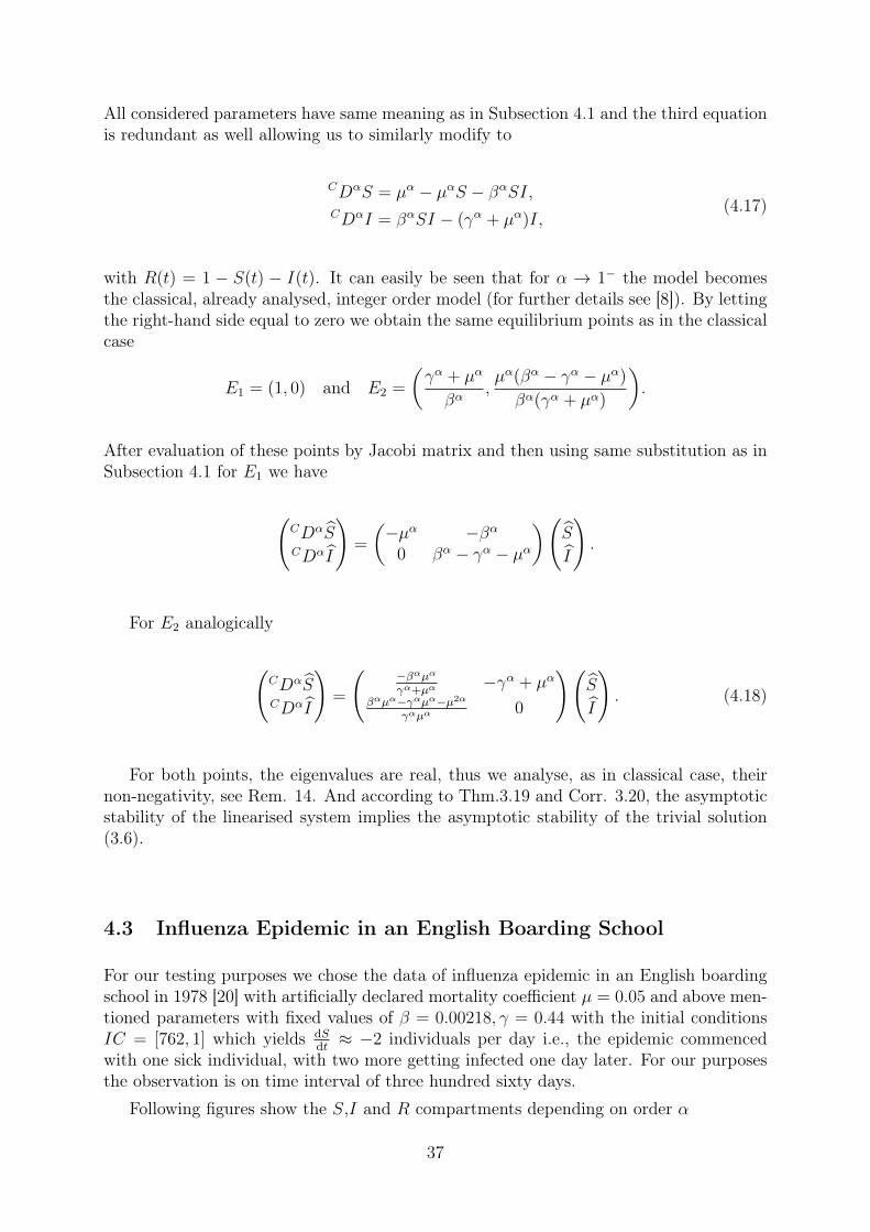
4.3 Influenza Epidemic in an English Boarding School

For our testing purposes we chose the data of influenza epidemic in an English boardingschool in 1978 [20] with artificially declared mortality coefficient µ = 0.05 and above men-tioned parameters with fixed values of β = 0.00218, γ = 0.44 with the initial conditionsIC = [762, 1] which yields dS

dt ≈ −2 individuals per day i.e., the epidemic commencedwith one sick individual, with two more getting infected one day later. For our purposesthe observation is on time interval of three hundred sixty days.

Following figures show the S,I and R compartments depending on order α

37

Figure 8: Susceptible and infected compartment, respectively.

38

Figure 9: SI phase plane

Figure 10: A closer detail of α ∈< 0.99; 0.92 >

39

Both, susceptible and infected, “compartments” show that with decreasing order αdecreases curvature and “creaseness” of the function for both cases until it smooths out.The recovered compartment does not change irregardless of order α, thus confirmingits redundancy. On our plots of the SI phase plane we can observe a transition fromstable focus equilibrium point to a stable node like one. Moreover, on the intervalα ∈< 0.99; 0.92 > we observe self-intersecting trajectories which occur no longer fromthe order α = 0.92 and less.

40

5 Numerical SolutionIn this Section we shall introduce a method applicable on wide range of equations dueto quite general assumptions. We shall focus on initial value problems with one Caputoderivative not limiting ourselves to only autonomous equations, however, we shall considerdimension n = 1 and α ∈ (0, 1), i.e.,

CDαy(x) = f(x, y(x)),

y(0) = y0

(5.1)

on finite interval [0, T ], where T is an adequate positive number.

5.1 The Predictor-Corrector Method

With help of Lem.3.13 we can state that solution of (5.1) is equivalent to the Volterraintegral equation

y(x) = y0 +1

Γ(α)

∫ x

0

(x− τ)α−1f(τ, y(τ))dτ (5.2)

with α ∈ (0, 1), meaning, that a continuous function is a solution of (5.1) if and only if itis a solution of (5.2).

Let us now recall the classical one-step Adams–Bashforth–Moulton for the first–orderequations. Assume an initial-value problem for the first–order differential equation

y′(x) = f(x, y(x)),

y(0) = y0

(5.3)

with such function f that a unique solution exists on some time interval [0, T ]. We shallalso assume a uniform grid τn = nh : n = 0, 1, . . . , N whereN is an arbitrary integer andh = T

N. The core idea is, assuming having already calculated approximations yh ≈ y(τi)

for (i = 1, 2, . . . , n), obtaining the approximation yh(τn+1) by means of the followingequation

y(τn+1) = y(τn) +

∫ τn+1

τn

f(u, y(u))du (5.4)

by integrating (5.3) on the interval [τn, τn+1]. Since we know none of the expressions onthe right–hand side of (5.4) precisely, we shall substitute y(τn) by known approximationyh(τn) instead. The integral is then replaced by trapezoidal quadrature formula thusgiving us the equation for the desired approximation as follows

yh(τn+1) = yh(τn) +h

2[f(τn, y(τn)) + f(τn+1, y(τn+1))], (5.5)

where y(τn) and y(τn+1 are replaced by their approximations yh(τn) and yh(τn+1), re-spectively. This provides us with with the implicit one-step Adams–Moulton method.However, the unknown yh(τn+1) appears on both sides and due to nonlinear characteris-tics of function f , we are, in general, unable to solve for yh(τn+1) directly. Nevertheless,we may use (5.5) in iterative process by inputting an estimate approximation for yh(τn+1)in the right-hand side for determination of better approximation which could be used.

41

The estimate approximation is so-called predictor and is obtained similarly with only dif-ference being replacing trapezoidal rule by rectangle one giving us the explicit or forwardEuler, or even one-step Adams–Bashforth method

yPh (τn+1) = yh(τn) + hf(τn, yh(τn)). (5.6)

This process and

yh(τn+1) = yh(τn) +h

2[f(τn, yh(τn)) + f(τn+1, y

Ph (τn+1))], (5.7)

known as the one–step Adams–Bashforth–Moulton method is convergent of order 2, i.e.,

maxn=1,2,...,N

|y(τn)− yh(τn)| = O(h2).

This method is said to be of the PECE (Predict, Evaluate, Correct, Evaluate) kindbecause, in our case we would, at first, calculate the predictor in equation (5.6), thenevaluate f(τn+1, y

Ph (τn+1)), using this for corrector calculation in equation (5.7), and at

last evaluating f(τn+1, yh(τn+1)).At this point we have introduced the essentials of the classical method. Now, our

attempt shall be to carry over these ideas to the fractional problems. Our main focusis to obtain an equation similar to (5.4). Such equation indeed exists, namely the (5.2),however, with one difference being the lower bound of integration starting at zero, notat τn which is a consequence of non-local structure of the Caputo differential operator.Nevertheless, this does not cause any serious problems in our generalisation of this method.We shall simply approximate the integral

∫ τn+1

0(τn+1−u)α−1g(u)du by substitution of the

function g with linear interpolant with knots chosen at τj (j = 0, 1, . . . , n + 1) and weshall use the product trapezoidal quadrature formula. In other words,∫ τn+1

0

(τn+1 − u)α−1g(u)du ≈ hα

α(α + 1)

n+1∑j=0

aj,n+1g(τj),

where

aj,n+1 =

nα+1 − (n− α)(n+ 1)α, if j=0,(n− j + 2)α+1 + (n− j)α+1 − 2(n− j + 1)α+1, if 1 ≤ j ≤ n,1, if j=n+1.

(5.8)

Now, we obtain the fractional variant of the one-step Adams-Moulton method, i.e.,the corrector formula, which is

yh(τn+1) = y0 +hα

Γ(n+ 2)f(τn+1, y

Ph (τn+1)) +

hα

Γ(n+ 2)

n∑j=0

aj,n+1f(τj, yh(τj)), (5.9)

where identity Γ(α + 1) = αΓ(α) was used and the fact that an+1,n+1 = 1.The remaining problem is to determine the predictor formula in order to evaluate

yPh (τn+1). The idea of generalisation of the one–step Adams–Bashforth method is identicalto one described above for the Adams–Moulton one, we replace the integral on the right–hand side of the equation (5.2) by the product rectangle rule, where now

bj,n+1 =hα

α((n+ 1− j)α − (n− j)α) (5.10)

42

and, therefore, the final formula for the predictor is

yPh (τn+1) = y0 +1

Γ(α)

n∑j=0

bj,n+1f(τj, yh(τj)). (5.11)

The fractional Adams–Bashforth–Moulton method is now fully described by equations(5.11) and (5.9) with weights aj,n+1 and bj,n+1 defined by (5.8) and (5.10), respectively.The error of this method is expected to behave as

max1≤j≤N

|y(τj)− yh(τj)| = O(hp),

wherep = min2, 1 + α.

The reason for this specific form of the exponent p is that it may be proved that p mustbe the minimum of the order of the corrector (2 in our case) and the predictor method(1 in our case) plus the order of the differential operator. For the case α = 1, the p = 2which is equivalent to the integer order method mentioned earlier.

Our description of the method can be easily expanded to the higher dimensions, i.e.,n ≥ 2, by replacing y ∈ R by the vector y ∈ Rn and instead of functions the vectorfunctions are considered.

43

6 SummaryIn this thesis we studied properties of autonomous systems, which are specific class ofdynamical ones. Our goal was to point out several differences between the classical, i.e.,first order systems and systems of fractional order between zero and one.

At the beginning we recalled some necessary definitions and theorems from the fieldof classical calculus. Here, we also mentioned techniques used for stability analysis ofnon-linear systems such as Routh–Hurwitz criterion, linearisation theorem and Lyapunovtheorem.

Then, in Section 3, we preliminarily recalled some higher functions and techniquesfrom classical calculus in order to introduce some standard approaches to the definitionof fractional derivatives and integrals, namely, the Riemann–Liouville and the Caputoapproach. This introduction was then followed by similar description of fractional au-tonomous systems and their stability. First of all, it is important to point out that in caseof fractional system no situation as periodic solution can occur, however, there are studiesof existence of asymptotic periodic solutions. Lastly, such phenomenon as self-intersectingtrajectories, namely, cusps and multiple points, may occur.

For verification of our theoretical results, the epidemiological SIR model with vitaldynamics, also referred to as Hethcote’s model, was chosen. In this thesis we focused onits local stability which was determined with help of linearisation theorem, Routh–Hurwitzcriterion, eigenvalues of characteristic equation of the system and, for the fractional case,the key factor of order α.

The analysis confirmed our expectation for fractional case that the stability remained.However, it turns out that a type transition of endemic equilibrium occurs, from stable fo-cus to stable node, to be precise, and even a self-intersecting phenomenon can be observedon the interval α ∈< 0.99; 0.93 >.

This work could be considered as rudimentary for further studies of epidemiologicalmodels, e.g., global stability of the SIR model and fractional dynamical systems, notnecessarily autonomous ones.

44

References[1] BHALEKAR, Sachin a Maddhuri PATIL. Singular points in the solution trajectories

of fractional dynamical systems. Chaos: An Indisciplinary Journal of Nonlinear sci-ence [online]. 2018, 28(11) [cit. 2020-06-19]. DOI: 10.1063/1.5054630. ISSN 1054-1500.Dostupné z: https://aip.scitation.org/doi/10.1063/1.5054630.

[2] BRAUER,Fred a CASTILLO-CHÁVEZ, Carlos.: Mathematical Models in PopulationBiology and Epidemiology. Springer, NY, 2012.

[3] CONG, Nguyen Dinh a Hoang The TUAN. Generation of nonlocal fractional dynam-ical systems by fractional differential equations. Journal of Integral Equations andApplications . 2017, 29(4), 585-608. ISSN 0897-3962.

[4] CONG, Nguyen Dinh, et al. Linearized asymptotic stability for fractional differentialequations. Electronic Journal of Qualitative Theory of Differential Equations . 2016,No. 39, 1-13. ISSN 1417-3875.

[5] ČERMÁK, Jan a Luděk NECHVÁTAL. Matematika III . Brno: Akademické naklada-telství CERM, 2016. ISBN 978-80-214-5400-2.

[6] ČULÍKOVÁ, Aneta. Epidemické dynamické modely [online]. Olomouc, 2017 [cit.2020-09-06]. Bakalářská práce. Univerzita Palackého v Olomouci, Přírodovědeckáfakulta. prof. RNDr. Irena Rachůnková, DrSc. Dostupné z: https://library.upol.cz/arl-upol/cs/csg/?repo=upolrepo&key=68788007971.

[7] DIETHELM, Kai. The Analysis of Fractional Differential Equations: An Applica-tion Oriented Exposition Using Differential Operators of Caputo Type. 2004. Berlin:Springer-Verlag, c2010. ISBN 978-3-642-14573-5.

[8] DIETHELM, Kai. A fractional calculus based model for the simulation of an out-break of dengue fever. Nonlinear Dynamics [online].2013, 71(4), 613-619. DOI:10.1007/s11071-012-0475-2.

[9] DIETHELM, Kai, Neville J. FORD a Alan D. FREED. A Predictor-Corrector Ap-proach for the Numerical Solution of Fractional Differential Equations. Nonlinear Dy-namics . 2002, 29(1–4), 3–22. ISSN 0924-090X.

[10] FEČKAN, Michal. Note on periodic solutions of fractional differential equations.Mathematical Methods in the Applied Sciences [online]. 2018, vol. 41, 5065-5073 [cit.2020-09-06]. DOI: 10.1002/mma.4953.Dostupné z: https://onlinelibrary.wiley.com/doi/abs/10.1002/mma.4953.

[11] FRANCŮ, Jan. Obyčejné diferenciální rovnice[online]. 2019-11-05. [cit. 2020-06-19].Dostupné z: https://math.fme.vutbr.cz/home/francu.

[12] HETHCOTE, Herbert W. The Mathematics of Infectious Diseases. SIAM Review[online]. 2000, 42(4), 599-653 [cit. 2020-06-19]. ISSN 1095-7200. Dostupné z: https://epubs.siam.org/doi/10.1137/S0036144500371907.

[13] KALAS, Josef a Zdeněk POSPÍŠIL. Spojité modely v biologii . Brno: Masarykovauniverzita, 2001. ISBN 80-210-2626-X.

45

[14] KISELA, Tomáš. Fractional Differential Equations and Their Applications Brno:Vysoké učení technické v Brně, Fakulta strojního inženýrství, 2008. 50 p. Vedoucídiplomové práce doc. RNDr. Jan Čermák, CSc.

[15] LAYEK G.C. An Introduction to Dynamical Systems and Chaos . New Delhi:Springer-India, c2015. ISBN 978-81-322-2555-3.

[16] LAZAREVIC, Mihailo P., et al. Advanced Topics on Applications of Fractional Cal-culus on Control Problems, System Stability and Modeling . WSEAS Press, 2014. ISBN978-960-474-348-3.

[17] MOUAOUINE, Abderrahim, et al. A fractional order SIR epidemic modelwith linear incidence rate. Advanaces in Difference Equations [online]. Vy-dáno: 03 May 2018, 160(2018) [cit. 2020-06-19]. ISSN 1687-1847. Dostupnéz: https://advancesindifferenceequations.springeropen.com/articles/10.1186/s13662-018-1613-z

[18] PERKO, Lawrence. Differential Equations and Dynamical Systems . 3rd ed. NewYork, NY: Springer New York, 2001. ISBN 0-387-95116-4.

[19] Free figure available from: https://i.stack.imgur.com/duPPi.png

[20] SULSKY, Deborah.Using Real Data in an SIR Model [online]. 2012. [cit. 2020-06-22].Dostupné z: https://www.math.unm.edu/~sulsky/mathcamp/ApplyData.pdf.

[21] WEISSTEIN, Eric W. Kermack-McKendrick Model. MathWorld-A Wolfram WebResource [online]. [cit 2020-06-23]. Dostupné z: https://mathworld.wolfram.com/Kermack-McKendrickModel.html.

46

Appendix

1 %% ''HETHCOTE'S'' FRACTIONAL SIR MODEL2 %% input (parameters of the system)3 %DATA: Influenza Epidemic in an English Boarding School, 19784 %LINK: https://www.math.unm.edu/¬sulsky/mathcamp/ApplyData.pdf5

6 N=763; % number of individuals in a population7 beta=0.00218; % proportionality for the disease transmission rate8 gam=0.44; % rate of recovery from the disease9 mu=0.05; % mortality coeffcient

10 alpha=1; % order of Caputo derivative11

12 %% output (SIR vector of the state variables)13 % S(t) - number of susceptibles at the time t14 % I(t) - number of infectives at the time t15 % R(t) - number of recovered individuals at the time t (R=N-S-I)16

17 %% numerical solution data18 t0=0; % initial time19 T=360; % final time20 h=0.001; % time step21 IC=[762;1]; % initial conditions vector22

23 fde = @(t,y)[-beta*y(1)*y(2)+mu*(N-y(1)) ; beta*y(1)*y(2)-(gam+mu)*y(2)];24

25 %% Fractional PECE method by R. Garrappa (fde12)26 [t,SI]=fde12(alpha,fde,t0,T,IC,h);27 %% plotting results28 %PHASE PORTRAIT29 plot(SI(1,:),SI(2,:), '-', 'color', 'black')30 legend('alpha=1','alpha=0.99','alpha=0.9','alpha=0.7','alpha=0.5','alpha=0.3')31 hold on32 grid on33 set(gca, 'FontName', 'Times New Roman')34 xlabel('S','FontName', 'Times New ...

Roman','FontAngle','italic','fontsize',12);35 ylabel('I','FontName', 'Times New ...

Roman','FontAngle','italic','fontsize',12);36 set(get(gca,'ylabel'),'rotation',0)37 hold off38

39 m=size(SI,2);40 NN=N*ones(1,m);41 R=NN-SI(1,:)-SI(2,:);42

43 % SIR figure44 plot(t,SI(1,:),t,SI(2,:),t,R)45 legend('S','I','R','Location','northeast','Orientation','vertical')46 grid on47 set(gca, 'FontName', 'Times New Roman')48 xlabel('t','FontName', 'Times New ...

Roman','FontAngle','italic','fontsize',12);49 ylabel('SIR','FontAngle', 'italic','fontsize',12)

47