Autonomous Transition Flight for a Vertical Take-Off and LandingAircraft

Pedro Casau

Abstract— This paper addresses modelling and control prob-lems for an model-scale Unmanned Air Vehicle (UAV) which isintended to perform Vertical Take-Off and Landing (VTOL)autonomously as well as transition to level flight. The firstcontribution of this thesis is the description of an accurate UAVnonlinear model which captures both hovering and level flightbehaviors. Furthermore, the Hybrid Automata framework isintroduced into the model by means of supervisory control whichprovides dynamics switching between modes of operation. Thesecond contribution concerns the problems of i) hover andlevel flight stabilization and, ii) Transition trajectory trackingby means of linear control techniques. Finally, a control lawwhich renders the system locally Input-to-State Stable (ISS) isdesigned within the Hybrid Systems’ framework allowing forpractical trajectory tracking.

I. INTRODUCTION

The demand for Unmanned Air Vehicles (UAVs) hasescalated in the past few years due to their contributions incommercial and defense applications, including fire surveil-lance and mitigation operations, agricultural fields spraying,infrastructure inspection, among others (see e.g. [1] and [2]).Several UAV configurations have been developed to meetthe requirements imposed by such applications, includingfixed-wing and tilt wing aircraft, rotorcrafts and ducted-fanvehicles.

Recent developments described in [3] have shown thatfixed-wing Vertical Take-Off and Landing (VTOL) aircraftscan perform both long endurance missions and precise ma-neuvering within exiguous environments. The versatility ofsuch aircrafts combines helicopter precise trajectory trackingwith conventional fixed-wing airplanes ability to cover largedistances, delivering a final solution which largely exceedsthe capabilities of its predecessors. However, the problemof achieving robust transitions between hover and leveledflights is difficult for its exquisite dynamics. To this end,several control methodologies have been employed, includ-ing robust linear control, feedback linearization techniquesand adaptive controllers (see e.g. [4] and [5]) but thesedifferent approaches still lack a formal proof of stability androbustness.

The very different aircraft dynamics between hover andleveled flights suggest that supervisory control (i.e. theapplication of different control techniques for each operatingmode) is a plausible solution for the given problem. Similarmethodologies, like the ones described in [6] and [7], havebeen successfully employed in a variety of applications.Controller switching during operating mode transitions addsdiscrete behavior to the continuous UAV model, creating anew layer of complexity which must be dealt appropriately.

Systems which display both continuous and discrete be-havior have been under an intense research effort over the last

decade. This study has given rise to several concepts suchas hybrid automata [8] and switched systems [9] which fallwithin the broader category of Hybrid Dynamical Systemsdescribed in [6]. The discrete behavior built into thesesystems may appear naturally for certain applications such asUAV landing and take-off (see e.g. [10]) but may also be theconsequence of digital control or supervisory control [11].

The solution proposed in this thesis employs supervisorycontrol by modeling the small-scale UAV within the HybridAutomata framework, dividing the aircraft flight envelopeinto Hover, Transition and Level operating modes. Linearoptimal control techniques are employed for system stabi-lization in hover and level flight while linear and nonlinearcontrol solutions are exploited for stabilization during tran-sition flight.

This paper is organized as follows. Section II presents the3-dimensional UAV nonlinear model, explaining thoroughlythe gravity, propeller and aerodynamic interactions withthe aircraft body while the Hybrid Automaton introducedin Section III models the switching events introduced bysupervisory control. Section IV presents the controller struc-tures which are employed during local stabilization and thetracking of the reference trajectories. Finally, Section Vpresents the nonlinear controller structure which renders theclosed-loop system Input-to-State Stable.

II. UAV NONLINEAR MODEL

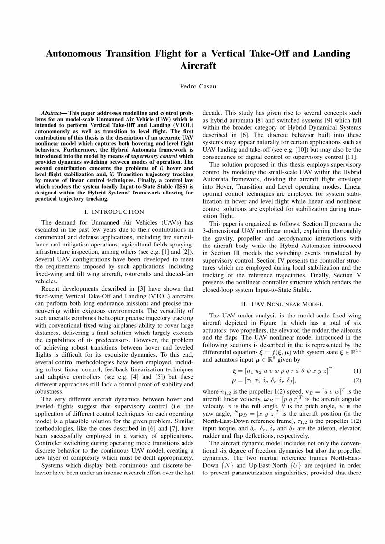
The UAV under analysis is the model-scale fixed wingaircraft depicted in Figure 1a which has a total of sixactuators: two propellers, the elevator, the rudder, the aileronsand the flaps. The UAV nonlinear model introduced in thefollowing sections is described in the is represented by thedifferential equations ξ = f(ξ,µ) with system state ξ ∈ R14

and actuators input µ ∈ R6 given by

ξ = [n1 n2 u v w p q r φ θ ψ x y z]T (1)µ = [τ1 τ2 δa δe δr δf ], (2)

where n1,2 is the propeller 1(2) speed, vB = [u v w]T is theaircraft linear velocity, ωB = [p q r]T is the aircraft angularvelocity, φ is the roll angle, θ is the pitch angle, ψ is theyaw angle, NpB = [x y z]T is the aircraft position (in theNorth-East-Down reference frame), τ1,2 is the propeller 1(2)input torque, and δa, δe, δr and δf are the aileron, elevator,rudder and flap deflections, respectively.

The aircraft dynamic model includes not only the conven-tional six degree of freedom dynamics but also the propellerdynamics. The two inertial reference frames North-East-Down N and Up-East-North U are required in orderto prevent parametrization singularities, provided that there

(a) Model-scale UAV picture (b) UAV model representation.

Fig. 1: The unmanned controlled vehicle.

exists appropriate switching between them. The North-East-Down reference frame N is located at some point on theEarth’s surface (which is assumed to be flat and still) and isdefined by the set of unitary vectors iN , jN ,kN where: iNis tangent to the earth’s surface and points to the geographicNorth; jN is normal to iN , tangent to the Earth’s surface andpoints to the East; kN completes the right handed set.

The Up-East-North reference frame U origin is coinci-dent with that of N and is defined by the set of unitaryvectors iU , jU ,kU where: kU is tangent to the earth’ssurface and points to the geographic North; jU is normalto kU , tangent to the Earth’s surface and points to the East;iU completes the right handed set.

The Body Reference Frame B has its origin in theaircraft center of gravity and is defined orthogonal and righthanded set of unitary vectors iB , jB ,kB which satisfy thefollowing specifications: iB is collinear with the aircraft’szero lift axis (roll axis); jB is normal to the symmetry plane(pitch axis); kB completes the right handed set (yaw axis).For the sake of simplicity, the Body Reference Frame isconsidered to be the principal axis of inertia.

The propellers, aerodynamic loads and gravity produce theforces and moments which affect the aircraft’s behavior.

The gravity field produces a force which is directedtowards the nadir and is given by

N fg = [0 0 mg]T , (3)U fg = [−mg 0 0]T , (4)

fg = BI R

Ifg , (5)

in the reference frames N, U and B, respectively.The gravity moment is null because the center of gravity(CG) is coincident with the center of mass (CM).

The propellers dynamics and thrust are mainly character-ized by their Coefficient of Thrust CT and Coefficient ofPower CP which are approximately given by

CT = CT0

(1− J

JM

), (6)

CP = CP0+

(J

JM

)2

(CPM − CP0), (7)

where J = u/nd is the propeller advance ratio, n is thepropeller’s speed, d is the diameter, CT0

is the Coefficientof Thrust at zero velocity, CP0 is the Coefficient of Powerat zero velocity, JM is the advance ratio of zero thrust andCPM is the Coefficient of Power at J = JM . CT and CPare related with the propeller’s thrust and power according

to

T =ρn2d4CT (J), (8)P =ρn3d5CP (J), (9)

where ρ is the atmospheric density. The propeller’s dynamicmodel is approximated by

Ip2πn = τ −Q, (10)

where Ip is its moment of inertia, τ is the input torque andQ is the aerodynamic drag torque acting on the propellerwhich is given by

Q =P

2πn. (11)

The set of moments acting on the aircraft body due to pro-peller rotation (mp) includes the acceleration torque (macc),the drag torque (mdrag), the gyroscopic torque (mgyro)and the displacement torque (mdis) which arises from thedisplacement rp of the propeller’s center with respect to thecenter of gravity. These torques are given by

mpi = macci + mdragi + mgyroi + mdisi , (12)(13)

where subscript i ∈ 1, 2 in the formulæ above distin-guishes each propeller and their moments’ sign changeaccording to the propeller’s rotation. The total thrust andtorque produced by the propellers is given by

fp =

Tp1 + Tp200

, (14)

mp =mp1 + mp2 . (15)

The aerodynamic forces are generated from the propellerslipstream flow and the free-stream flow. The two contribu-tions are calculated separately and combined together in theend using superposition. Under this assumption, the propellerslipstream velocity up is given by

up =

√8T

ρπd2, (16)

considering a steady, incompressible and inviscid flow.The lifting surfaces’ lift Li and drag Di is given by the

following equations for any u ≥ 0

Li =1

2ρAiu

2∞CLi , (17)

Di =1

2ρAiu

2∞CDi , (18)

where Ai is the surface’s planform area and u∞ = u underthe small angle approximation. These aerodynamic forcesgreatly depend on the surface’s Coefficient of Lift (CL) andthe Coefficient of Drag (CD), which are described by

CL = CL(α, δj), (19)

CD = CD0+

C2L

πAe, (20)

where α = arctan(w/u) is the surface’s angle of attack1, δjis the actuator deflection, CD0 is the parasitic Coefficient of

1For the vertical stabilizer the sideslip angle β = arcsin(v/‖vB‖) isused instead of the angle of attack

Drag,A is the aspect ratio and e is the Oswald’s efficiency.The Coefficient of Lift is given by

CL =

CLαα+ CLδj δj , if − CLmax ≤ CL ≤ CLmax0, otherwise

.

(21)CL is lower bounded at −CLmax and upper bounded atCLmax . These limits induce loss of lift (stall) at angles ofattack such that α /∈ [α, α] where CL(α) = CLmax andCL(α) = −CLmax . Applying (17) and (18) to the wing,horizontal stabilizer and vertical stabilizer one computes theLift and Drag forces acting on the aircraft body Lw, Dw,Lhs, Dhs, Lvs and Dvs. Thus, the aerodynamic forces actingon the aircraft are given by (22) under the small angleapproximation.

fa =

Dw +Dhs +Dvs

LvsLw + Lhs

(22)

The aerodynamic moment ma calculation requires the esti-mation of the aileron’s mean pressure center location (ra), itsslipstream mean pressure center (rp,a) location, the horizon-tal stabilizer’s aerodynamic center location (rhs), the wing’saerodynamic center location (rw) and the vertical stabilizer’saerodynamic center location (rvs). Given these parameters itis then computed by

ma = mw + mhs + mvs +

Ma

Mdampq

Mdampr

, (23)

where Ma, mhs, mvs, mw, Mdampq and Mdampr define theaileron moment, the elevator moment, the rudder moment,the wing moment and the damping moments due to pitchand yaw rotation, respectively. The previously defined forcesand moments complete the dynamic model description. Thenext section formulates the UAV Hybrid Automaton whichaccounts for controller switching during operating modetransitions.

III. HYBRID AUTOMATON

The system’s discrete behavior is captured by means of aHybrid Automaton which is identified by: a set of the Oper-ating Modes Q; a Domain Mapping D : Q⇒ Rn × Rm; aFlow Map f : Q × D → Rn; a set of Edges E ⊂ Q × Q;a Guard Mapping G : E ⇒ Rn × Rm and; a Reset MapR : E ×Rn ×Rm → Rn (see [8] or [6] for further details).The system state ξ ∈ R14 is defined in (1) and the actuatorinput µ ∈ R7 is given by

µ = [τ1 τ2 δa δe δr δf q∗]T , (24)

where a new input variable q∗ ∈ Q∗ = H,L to informthe controller which is the desired Operating Mode andwhether transition is required. The remaining state and inputvariables were defined in Section II.The Hybrid Automatonrepresentation is provided in Figure 2.

A. Operating ModesThe Hybrid Automata operating mode q must belong to

the set Q = H,X,L which has the meaning• H - Hover operating mode with Hover controller se-

lected, i.e. µ = µH(ξ, ξ∗(t));

• X - Transition operating mode with Transition con-troller selected, i.e. µ = µX(ξ, ξ∗(t));

• L - Level operating mode with Level controller selected,i.e. µ = µL(ξ, ξ∗(t));

The variable ξ?(t) represents the reference state trajectorywhich the controller is tracking.

B. Domain MappingFor each Operating Mode, the domain mapping D : Q⇒

R14 × R6 × Q∗ assigns the set where the variables (ξ,µ)may range and it is defined by2

D(H) =[nmin, nmax]2 × R6 ×BφH (0)×BθH (0)×BψH (0)× R2 × R≤0 × U

D(X) =[nmin, nmax]2 × R≥0 × R5 ×BφX (0)×BθX (0)×BψX (0)× R2 × R<0 × U

D(L) =[nmin, nmax]2 × R>0 × R5 ×BφL(0)×BθL(0)×

BψL(0)× R2 × R<0 × U⋂

(u,w) ∈ R>0 × R : α < arctan(w/u) < α(25)

where the actuators domain is the set U ⊂ R3 × Q∗ givenby

U =[τmin, τmax]2 × [δamin , δamax ]× [δemin , δemax ]×[δrmin , δrmax ]× [δfmin , δfmax ]×Q∗

(26)The angle limits φH , φL, θH , θL, ψH and ψL are requiredfor the Hover and Level Operating Modes domains to liewithin the corresponding basin of attraction, i.e. if Bq is thebasin of attraction for the operating mode q then D(q) ⊂ Bq .

C. Flow MapThe Flow Map f : Q × R14 × U → R6 describes the

evolution of the state variables in each operating mode q ∈Q, i.e. in each operating mode the state’s derivative is givenby

ξ = f(q , ξ,µq ) (27)

where function f is the set of differential equations whichdescribe the aircraft dynamic model.

D. EdgesThe set of edges E ⊂ Q × Q identifies any operating

mode transition from q1 to q2 represented in Figure 2 withthe pair (q1, q2). The possible operating mode transitions inthis model are: (H,X), (X,L), (L,X) and (X,H).

2Bε(p) represents a ball of radius ε around the point p, i.e. the set ofpoints x such that ‖x− p‖ < ε.

HOVER TRANSITION LEVEL

Fig. 2: The UAV Hybrid Automaton

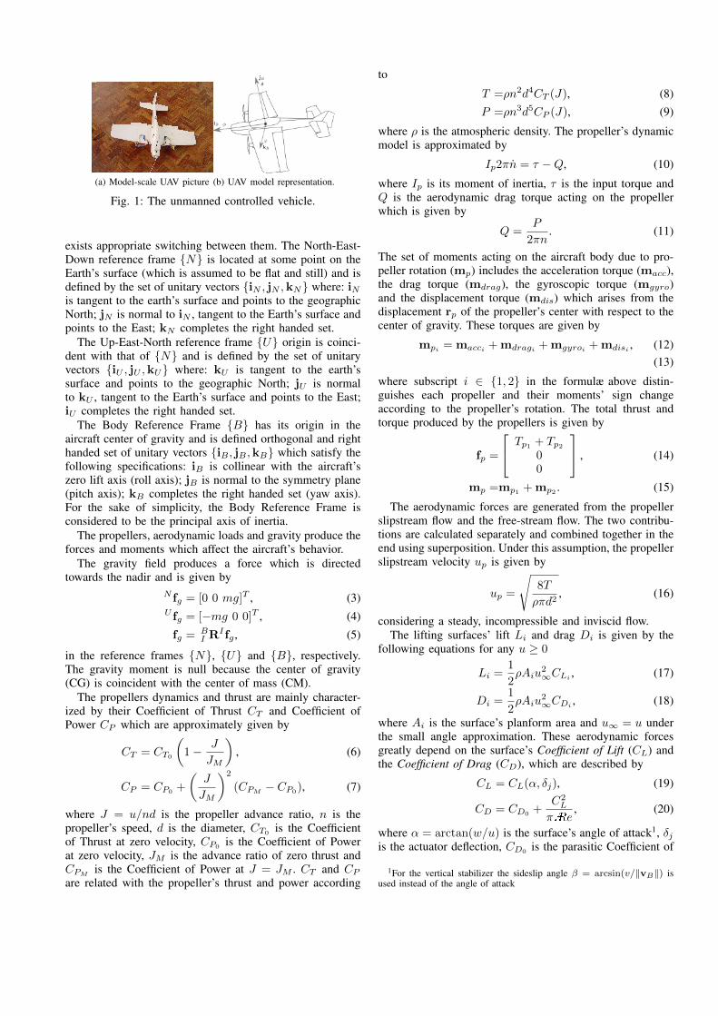
E. Guard Mapping

The Guard Mapping G : E ⇒ R14 × R6 ×Q∗ determinesfor each pair (q1, q2) the set to which the aircraft state mustbelong in order to perform the transition. The switch fromHover to the Transition operating mode is performed onlyif the aircraft state verifies the controller restrictions on theinitial state which are denoted by χH→X . Therefore, givena Transition to Level approach trajectory

v?X→L(t) = (ξ?X→L(t), µ?X→L(t)),

switching from Hover to Transition occurs when the aircraftstate is χH→X -close to v?X→L(0). The guard mapping issimilarly defined for the switch from Level to Transition.

Switching from Transition to either Hover or Level oper-ating modes is performed whenever the aircraft state belongsto some set

Xq ⊂ D(q) (28)

where q ∈ H,L. Under the previous considerations, theGuard Mapping is defined by

G(H,X) =BχH→X(v∗X→L(0))

G(X,L) =

(ξ,µ) ∈ D(L) : |φ| ≤ φX→L∧

|θ| ≤ θX→L ∧ |ψ| ≤ ψX→L ∧ q∗ = L

G(L,X) =BχL→X(v∗X→H(0))

G(X,H) =

(ξ,µ) ∈ D(L) : |φ| ≤ φX→H∧

|θ| ≤ θX→H ∧ |ψ| ≤ ψX→H ∧ q∗ = H

(29)

where the pitch angle boundaries φX→L, θX→L, ψX→L,φX→H , θX→H and ψX→L must verify

φX→L < φL θX→L < θL ψX→L < ψL

φX→H < φH θX→H < θH ψX→H < ψH

in order to meet the condition (28). A guard mappingrepresentation is given in Figure 3.

F. Reset Map

For each (q1, q2) ∈ E and (ξ, µ) ∈ G(q1, q2), the resetmap R : E ×R14×U → R14 identifies the jump of the statevariable ξ during the operating mode transition from q1 toq2. State changes occur when switching from Transition toLevel due to different attitude parametrization between the

Fig. 3: Guard mapping representation

operating modes. The reset map is given byR(H,X) =ξ,

R(X,L) =[n1 n2 u v w p q r arctan(BNR23/BNR33)

arcsin(−BNR13) arctan(BNR12/BNR11) x y z]T ,

R(L,X) =[n1 n2 u v w p q r arctan(BUR23/BUR33)

arcsin(−BUR13) arctan(BUR12/BUR11) x y z]T ,

R(X,H) =ξ,(30)

where the symbol Rij is the matrix R element which isfound at the i-th row and j-th column.

IV. LINEAR QUADRATIC REGULATOR

A. Controller StructureThe LQR control structure has already been extensively

studied and is categorized as very reliable, for it has highgain and phase margins [12]. This control solution requiresthe system to be linear, however it has been proved thatstabilization of a nonlinear system is also feasible withina neighborhood of the equilibrium point [13]. Classic LQRtechniques provide the full state feedback control law µ =−Kξ which robustly stabilizes the aircraft within a sublevelset of the Lyapunov function V ξ) = ξT ξ near the lineariza-tion point (ξ0,µ0), where ξ = ξ − ξ0 and µ = µ− µ0.

Each operating mode has a different operating point andspecifications which require distinct weightings. Thereforecontroller dimensioning requires:

1) Linearization around the chosen operating point(ξq ,µq );

2) Integrator states (ξ) choice according to the operatingmode requirements;

3) Controllability evaluation;4) (Q,R) weighting using Bryson’s trial-and-error

method, which employs the diagonal matrices

Q =

∆ξ−21max . . . 0...

. . ....

0 . . . ∆ξ−2nmax

, (31)

R =

∆µ−21max

. . . 0...

. . ....

0 . . . ∆µ−2mmax

, (32)

where ∆ξimax represents the i-th state maximum ex-pected deviation from equilibrium and ∆µjmax repre-sents the j-th input maximum expected deviation fromequilibrium.

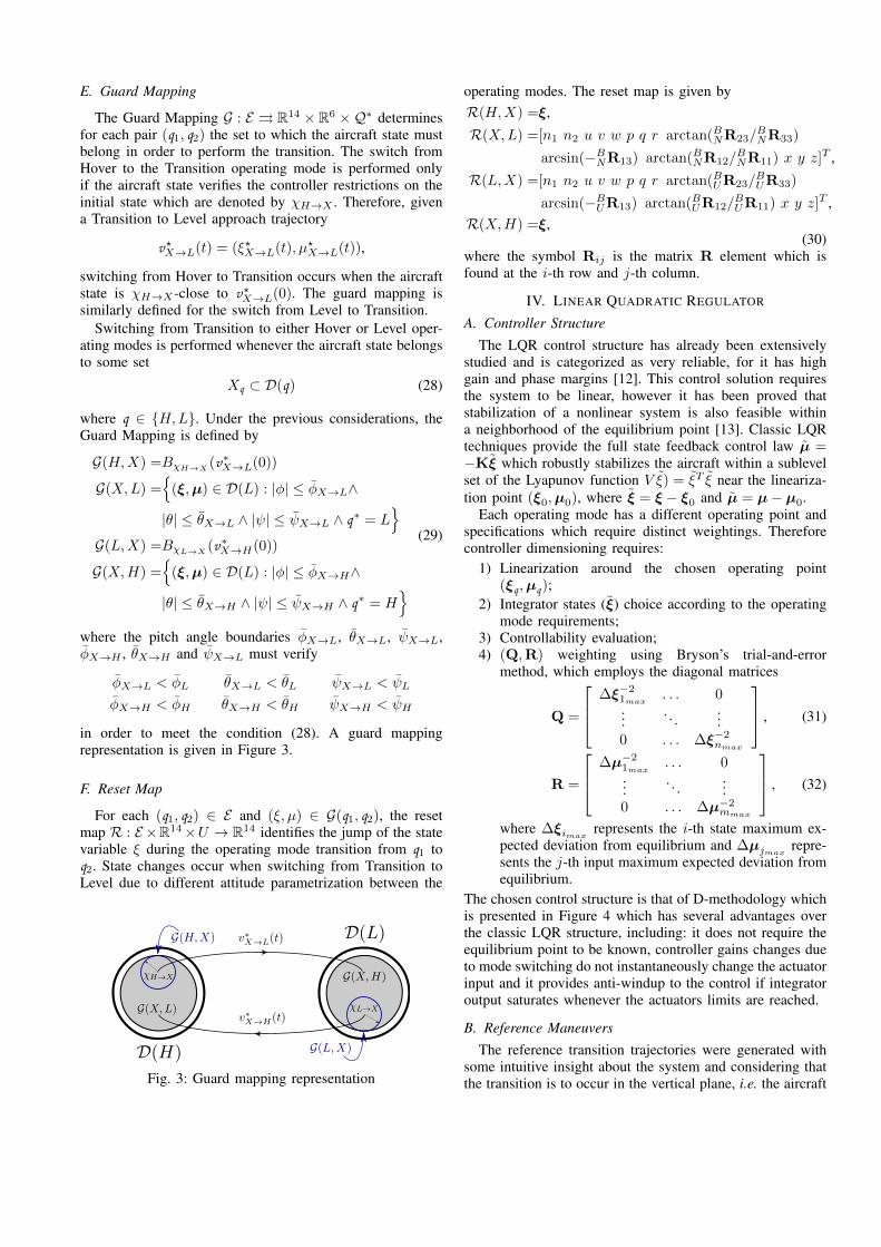
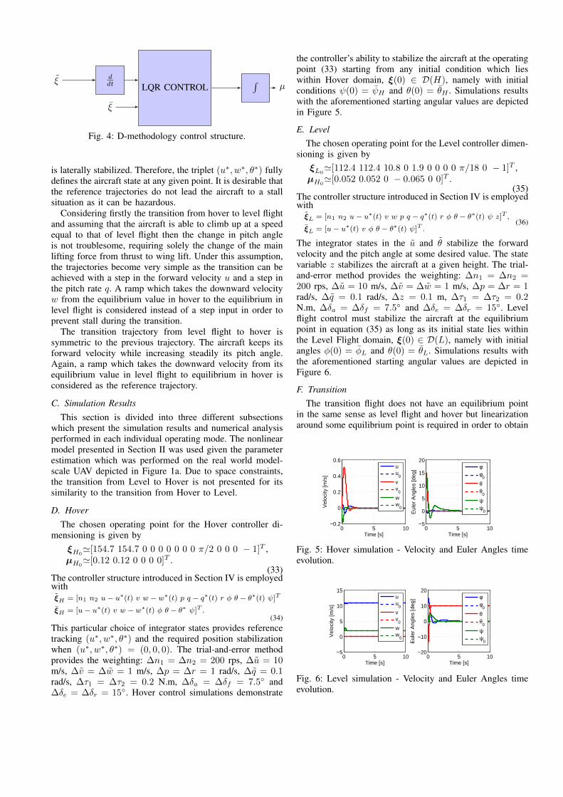
The chosen control structure is that of D-methodology whichis presented in Figure 4 which has several advantages overthe classic LQR structure, including: it does not require theequilibrium point to be known, controller gains changes dueto mode switching do not instantaneously change the actuatorinput and it provides anti-windup to the control if integratoroutput saturates whenever the actuators limits are reached.

B. Reference ManeuversThe reference transition trajectories were generated with

some intuitive insight about the system and considering thatthe transition is to occur in the vertical plane, i.e. the aircraft

ξ ddt

ξ

LQR CONTROL∫

µ

Fig. 4: D-methodology control structure.

is laterally stabilized. Therefore, the triplet (u∗, w∗, θ∗) fullydefines the aircraft state at any given point. It is desirable thatthe reference trajectories do not lead the aircraft to a stallsituation as it can be hazardous.

Considering firstly the transition from hover to level flightand assuming that the aircraft is able to climb up at a speedequal to that of level flight then the change in pitch angleis not troublesome, requiring solely the change of the mainlifting force from thrust to wing lift. Under this assumption,the trajectories become very simple as the transition can beachieved with a step in the forward velocity u and a step inthe pitch rate q. A ramp which takes the downward velocityw from the equilibrium value in hover to the equilibrium inlevel flight is considered instead of a step input in order toprevent stall during the transition.

The transition trajectory from level flight to hover issymmetric to the previous trajectory. The aircraft keeps itsforward velocity while increasing steadily its pitch angle.Again, a ramp which takes the downward velocity from itsequilibrium value in level flight to equilibrium in hover isconsidered as the reference trajectory.

C. Simulation ResultsThis section is divided into three different subsections

which present the simulation results and numerical analysisperformed in each individual operating mode. The nonlinearmodel presented in Section II was used given the parameterestimation which was performed on the real world model-scale UAV depicted in Figure 1a. Due to space constraints,the transition from Level to Hover is not presented for itssimilarity to the transition from Hover to Level.

D. HoverThe chosen operating point for the Hover controller di-

mensioning is given byξH0'[154.7 154.7 0 0 0 0 0 0 0 π/2 0 0 0 − 1]T ,

µH0'[0.12 0.12 0 0 0 0]T .

(33)The controller structure introduced in Section IV is employedwithξH = [n1 n2 u− u∗(t) v w − w∗(t) p q − q∗(t) r φ θ − θ∗(t) ψ]T

ξH = [u− u∗(t) v w − w∗(t) φ θ − θ∗ ψ]T .(34)

This particular choice of integrator states provides referencetracking (u∗, w∗, θ∗) and the required position stabilizationwhen (u∗, w∗, θ∗) = (0, 0, 0). The trial-and-error methodprovides the weighting: ∆n1 = ∆n2 = 200 rps, ∆u = 10m/s, ∆v = ∆w = 1 m/s, ∆p = ∆r = 1 rad/s, ∆q = 0.1rad/s, ∆τ1 = ∆τ2 = 0.2 N.m, ∆δa = ∆δf = 7.5 and∆δe = ∆δr = 15. Hover control simulations demonstrate

the controller’s ability to stabilize the aircraft at the operatingpoint (33) starting from any initial condition which lieswithin Hover domain, ξ(0) ∈ D(H), namely with initialconditions ψ(0) = ψH and θ(0) = θH . Simulations resultswith the aforementioned starting angular values are depictedin Figure 5.

E. LevelThe chosen operating point for the Level controller dimen-

sioning is given byξL0'[112.4 112.4 10.8 0 1.9 0 0 0 0 π/18 0 − 1]T ,

µH0'[0.052 0.052 0 − 0.065 0 0]T .

(35)The controller structure introduced in Section IV is employedwith

ξL = [n1 n2 u− u∗(t) v w p q − q∗(t) r φ θ − θ∗(t) ψ z]T ,

ξL = [u− u∗(t) v φ θ − θ∗(t) ψ]T .(36)

The integrator states in the u and θ stabilize the forwardvelocity and the pitch angle at some desired value. The statevariable z stabilizes the aircraft at a given height. The trial-and-error method provides the weighting: ∆n1 = ∆n2 =200 rps, ∆u = 10 m/s, ∆v = ∆w = 1 m/s, ∆p = ∆r = 1rad/s, ∆q = 0.1 rad/s, ∆z = 0.1 m, ∆τ1 = ∆τ2 = 0.2N.m, ∆δa = ∆δf = 7.5 and ∆δe = ∆δr = 15. Levelflight control must stabilize the aircraft at the equilibriumpoint in equation (35) as long as its initial state lies withinthe Level Flight domain, ξ(0) ∈ D(L), namely with initialangles φ(0) = φL and θ(0) = θL. Simulations results withthe aforementioned starting angular values are depicted inFigure 6.

F. TransitionThe transition flight does not have an equilibrium point

in the same sense as level flight and hover but linearizationaround some equilibrium point is required in order to obtain

0 5 10−0.2

0

0.2

0.4

0.6

Time [s]

Vel

ocity

[m/s

]

uu

0

vv

0

ww

0

0 5 10−5

0

5

10

15

20

Time [s]

Eul

er A

ngle

s [d

eg]

φφ

0

θθ

0

ψψ

0

Fig. 5: Hover simulation - Velocity and Euler Angles timeevolution.

0 5 10−5

0

5

10

15

Time [s]

Vel

ocity

[m/s

]

uu

0

vv

0

ww

0

0 5 10−20

−10

0

10

20

Time [s]

Eul

er A

ngle

s [d

eg]

φφ

0

θθ

0

ψψ

0

Fig. 6: Level simulation - Velocity and Euler Angles timeevolution.

the Transition controller. The chosen operating point givenin (37) is very similar to the Hover operating point. However,its forward velocity of 1 m/s provides the linear model withcharacteristics which are present both in hover and levelflight.

ξX0'[157.3 157.3 1 0 0 0 0 0 0 π/2 0 0 0 − 1]T

µX0'[0.12 0.12 0 0 0 0]T

(37)Again, the controller structure described in Section IV isemployed with

ξX = [n1 n2 u− u∗(t) v w − w∗(t) p q − q∗(t) r φ θ − θ∗(t) ψ]T

ξX = [u− u∗(t) v w − w∗(t) φ θ − θ∗ ψ]T ,(38)

which is equal to the choice made for the Hover controller.However, the transition flight controller spans a large set ofoperating points which are defined by the reference maneu-vers thus requiring different LQR weightings. The chosenweightings are ∆n1 = ∆n2 = 200 rps, ∆u = ∆v = ∆w =10 m/s, ∆p = ∆r = ∆q = 1 rad/s, ∆τ1 = ∆τ2 = 0.2 N.m,∆δa = ∆δf = 7.5, ∆δe = 15 and ∆δr = 45. Simulationresults show that the controller is able to stabilize the aircraftfor the whole flight envelope. However, this feature comes atthe cost of a more loosen reference tracking than that whichis provided during hover and level flight.

1) Transition: Hover to Level: The aircraft starts itstransition to level flight at the Hover equilibrium point and,since the reference transition trajectory starts at u = 1 m/s,a step input with the same magnitude is required when inHover. Figure 7 depicts the reference trajectory tracking andFigure 8 depicts the actuator inputs. The aircraft starts inHover, switches to Transition at time t = 0.9 s when theaircraft state enters the guard map D(H,X) and switches toLevel at t = 9.6 s when the guard map D(X,L) is breached.Nonlinear behavior is highly noticeable during switchingfrom Hover to Transition due to input torque saturation.The lateral variables are not presented because the deviationsfrom the vertical plane (x, z) are negligible.

V. NONLINEAR CONTROL

Despite the linear control solution feasibility, nonlinearcontrol techniques are also exploited. However, due toits inherent complexity, model simplification is performedin Section V-A before the controller design provided inSection V-C. The nonlinear controller is tested within the

0 5 10 150

7.5

15 H X L

Time [s]

For

war

d/D

ownw

ard

velo

city

[m/s

]

0 5 10 150

50

100

Pitc

h an

gle

[deg

]

u(t)

u*(t)w(t)

w*(t)θ(t)

θ*(t)

Fig. 7: Transition from Hover to Level simulation - referencetracking.

simulation environment against the full aircraft model.Theresults are presented in V-D.

A. Simplified Model

The following simplifications are applied to the aircraftmodel presented in Section II:• Propellers’ dynamics are neglected. The thrust they

provide is given by T = T1+T2

2 ;• Lateral motion is stabilized which in turn implies thatT1 − T2, δa, δr, v, p, r and y are null;

• The stall angle does not depend on the actuator deflec-tion but only on the angle of attack which must verify|α| < α, where α = 15 ;

• The horizontal and vertical stabilizers drag as well asthe flap contribution to the wing drag are neglected.

Under the previous assumptions, the configuration of thebody frame B with respect to N can be viewed asan element of the Special Euclidean group, (R,p) =(NBR,NpB) ∈ SE(2) where

NpB = [x z]T , NBR =

[cos θ sin θ

− sin θ cos θ

], (39)

thus eliminating the singularity in the rotation matrixparametrization which occurs in three-dimensional rotations.The kinematics are described by

N pB = NBRvB , θ = q, (40)

where NpB = [x z]T and vB = [u w]T . Under theprevious considerations, the main forces acting on the aircraftbody are the wing lift Lw, the horizontal stabilizer lift Lhsand the wing drag Dw. The lifting forces Lhs and Lwproduce the moments Mhs and Mw, respectively, due totheir displacement with respect to the center of gravity. Themoment Mdampq remains valid in this analysis. The actuatorsinput variables δe and δf can be changed into forces Le andLf , respectively, according to (41) and (42).

δe = − Le12ρ(2u2

p)Ap,hsCLδep,hs+ 1

2ρu2AhsCLδehs

(41)

δf = − Lf12ρ(2u2

p)Ap,wCLδfp,w+ 1

2ρu2AwCLδfw

(42)

0 5 10 15−10

−5

0

5

Time [s]

Ele

vato

r/F

lap

defle

ctio

n [d

eg]

H X L0 5 10 15

0

0.1

0.2

0.3

Inpu

t tor

que

[N.m

]

δe(t)

δf(t)

τ1(t)

τ2(t)

Fig. 8: Transition from Hover to Level simulation - actuatorinputs.

The dynamics equations are rewritten in (43) for the longi-tudinal case, under the aforementioned simplifications.

u =2T

m+ hu(u,w, q, θ),

w =Lf + Le

m+ hw(u,w, q, θ),

q = −rw. iBLf + rhs. iBLeIy

+ hq(u,w, q),

θ = q.

(43)

The new state variable to be monitored is

ξ = [u w q θ x z]T ,

thus, the Hybrid Automaton described in Section III isrequired to change in order to meet the specified simplifi-cations.

B. Robust Maneuvers

The problem of achieving robust transitions between hoverand level flights is twofold: i) the reference maneuver whichlinks the two sets must be at least ε-distant from the domainlimits and any guard sets leading to undesired operativemode transitions; ii) the controller must be able to achievepractical reference trajectory tracking with an error no largerthan ε, in the presence of external disturbances and uncertainparameters.

Three different kinds of robust maneuvers are definedwithin the Hybrid Automata framework.The first one, whichis denoted as ε-robust q1-single maneuver in [t0, t1), is suchthat the state and the input do not intersect any guard condi-tion in order to maintain the same "single" operating modeq1. The second type, denoted as ε-robust q1 → q2 approachmaneuver in [t0, T ], is such that at time T the maneuverbelongs robustly to the desired guard set, G(q1, q2), inorder to switch to the operating mode q2. The last one, theq1 → q2 transition maneuver in [t0, t1), is obtained as acombination of an ε-robust q1 → q2 approach maneuver anda set of ε-robust q2-single maneuvers.

Although q1-single maneuvers and q1 → q2 transitionmaneuvers are defined for the hybrid automaton presented inSection III, the most important maneuvers are the X → Land X → H approach maneuvers which are identifiedby v?X→L(t) and v?X→H(t), respectively. These referencemaneuvers are computed by means of system inversion.Given twice differentiable desired state trajectories u?(t)and θ?(t), the downward velocity initial state w?(0) andconsidering the flaps nominally at rest, i.e. L?f (t) = 0 for allt ≥ 0, then the reference control inputs T ?(t) and L?e(t), andthe reference state variable w?(t) are computed numericallyby solving (43).

C. Controller Design

The controller design comprises two different methods:linear optimal control techniques are used when in Hover orLevel operating modes, providing local stabilization; nonlin-ear control is used to perform the transition between the twodisjoint operating modes.

In order to build the nonlinear controller and prove theoverall system stability and robustness the state equations

are rewritten in a simpler form by substituting the relations[LM

]=

[1 1

−rhs. iB −rw. iB

] [LeLf

](44)

into (43). This substitution effectively rescales the controlinput throughout the maneuver. The new control input isdescribed by

µ =

T ?(t) + T

M?(t) + M

L?(t) + L

,

T = −kuuM = −kθ(θ + kq q)

L = −kww, (45)

where T ?(t), M?(t) and L?(t) are the reference inputs ob-tained by model inversion as explained in Section V-B and T ,M and L are the errors which result from practical referencetracking. Proportional-derivative (PD) controllers are usedto track the reference trajectories. Substituting (45) into thesystem state equations (43), the aircraft error dynamics aredescribed by

˙u =2T

m+ Ψu(u, w, q, θ, t) + δu(t), (46a)

˙w =L

m+ Ψw(u, w, q, θ, t) + δw(t), (46b)

˙q =M

Iy+ Ψq(u, w, q, t) + δq(t), (46c)

˙θ =q, (46d)

where the functions Ψu, Ψw and Ψq described by (47) havebeen introduced and the perturbation terms δu(t), δw(t) andδq(t) have been added. These perturbations may appear dueto parametric uncertainty, external disturbances and/or dueto deviations from the vertical plane.

Ψu(u, w, q, θ, t) =hu(u?(t) + u, w?(t) + w, q?(t) + q, θ + θ)

− hu(u?(t), w?(t), q?(t), θ?(t))

Ψw(u, w, q, θ, t) =hw(u?(t) + u, w?(t) + w, q?(t) + q, θ + θ)

− hw(u?(t), w?(t), q?(t), θ?(t))

Ψq(u, w, q, t) =hq(u?(t) + u, w?(t) + w, q?(t) + q)

− hq(u?(t), w?(t), q?(t))

(47)

The reference trajectory is one of equilibrium (if δu = δw =δq = 0) because

[u w q θ] = [0 0 0 0]⇒ [ ˙u ˙w ˙q˙θ] = [0 0 0 0].

The previous set of equations provides the foundationsupon which the nonlinear controller’s robustness emerges.Consider two separate but interconnected systems whichdescribe the pairs (u, w) and (θ1, θ2), where θ1 = θ andθ2 = q+ θ

kq. Input-to-State Stability is proven firstly for each

of these system separately in Propositions 1 and 2. Input-to-State Stability for the overall system then follows fromthe Small Gain Theorem described in both [14] and [15],which is applied to the feedback interconnection depicted inFigure 9.

Proposition 1: For some c?u > 0 and c?w > 0 and anynumbers satisfying ∆ > 0, ‖(θ1, θ2)‖ > 0, 0 < cu < c?u and0 < cw < c?w there exist ku > k?u and kw > k?w such that thesystem with the dynamics (46a) and (46b) is rendered ISSwith restrictions cu in the initial state u(0), cw on the initialstate w(0), ∆ on the inputs δu(t) and δw(t) and ‖(θ1, θ2)‖on the input (θ1(t), θ2(t)).

Proof: Consider the Lyapunov function (48) and thelevel set definition given in (49).

V1(u, w) =1

2(u2 + w2) (48)

Ω1(l) = (u, w) ∈ R2 : V1(u, w) ≤ l (49)(50)

It turns out that, due to radial unboundedness there existpositive l1 such that

(u, w) ∈ R2 : |u| ≤ cu ∧ |w| ≤ cw ⊂ Ω1(l1). (51)

Moreover, for any given reference trajectory it is possible tofind c?u, c?w and l?1 such that

(u, w) ∈ R2 : |u| ≤ c?u ∧ |w| ≤ c?w ⊂ Ω1(l?1), (52)and

(u, w) ∈ Ω1(l?1) : u?(t) + u > 0 ∧∣∣∣∣arctan

(w?(t) + w

u?(t) + u

)∣∣∣∣ < α

,

(53)hold true for all t ≥ 0.

The functions defined in (47) are locally Lipschitzbecause the functions hu, hw and hq are continuous andproper, therefore there exist positive Lu and Lw such thatfor all (u, w) ∈ Ω1(l1) and ‖(θ1(t), θ2(t))‖ < ‖(θ1, θ2)‖the following holds∥∥∥∥Ψu

(u, w, θ2 −

θ1

kq, θ1, t

)∥∥∥∥ ≤ Lu‖(u, w, θ1, θ2, t)‖, (54)∥∥∥∥Ψw

(u, w, θ2 −

θ1

kq, θ1, t

)∥∥∥∥ ≤ Lw‖(u, w, θ1, θ2, t)‖, (55)

for all t ≥ 0. The Lyapunov function derivative V1 is givenby

V1 = u

(−2kum

u+ Ψu

(u, w, θ2 −

θ1

kq, θ1, t

)+ δu(t)

)+ w

(−kwmw + Ψw

(u, w, θ2 −

θ1

kq, θ1, t

)+ δw(t)

).

(56)Substituting (54) and (55) into (56) and using the triangleinequality, the Lyapunov function’s derivative can be upperbounded by

V1 ≤− λmin‖(u, w)‖2 + ‖(u, w)‖((Lu + Lw)‖(θ1, θ2)‖++ δu(t) + δw(t)),

(57)where λmin is the smallest eigenvalue of the matrix[

2kum + Lu ± 1

2 (Lu + Lw)± 1

2 (Lu + Lw) kwm + Lw

].

(u, w)(δu(t), δw(t))

(θ1, θ2)δq(t)

Fig. 9: Interconnected systems (u, w) and (θ1, θ2).

It is easy to verify that for any ∆ > 0 and ‖(θ1, θ2)‖ >0 there exist k?w > 0 and k?u(k?w) > 0 such that for anyku > k?u, kw > k?w, (δu(t), δw(t)) satisfying ‖δu(t)‖∞ ≤ ∆,‖δw(t)‖∞ ≤ ∆, and ‖(θ1(t), θ2(t))‖∞ < ‖(θ1, θ2)‖ and forany (u, w) ∈ Ω1(l1) the following holds

V1 < 0 if ‖(u, w)‖ >Lu + Lw

λmin‖(θ1(t), θ2(t))‖+

δu(t) + δw(t)

λmin. (58)

The system has a local ISS function, therefore it is ISS withrestrictions cu on the initial state u(0), cw on the initial statew(0) and ∆ on the inputs δu(t) and δw(t) as long as theconditions cu < c?u and cw < c?w are satisfied.

Proposition 2 employs similar arguments to those in Propo-sition 1 proof in order to justify the Input-to-State Stabilityof the closed-loop system (θ1, θ2).

Proposition 2: For any arbitrary positive numbers ∆,‖u, w‖, kq , cq and cθ there exists k?θ(kq) > 0 suchthat kθ > k?θ renders the system with the dynamics (46a)and (46b) ISS with restrictions cq on the initial state q(0),cθ on the initial state θ(0), ‖u, w‖ on the input (u(t), w(t))and ∆ on the input δq(t).

Proof: Consider the Lyapunov function describedby (59) and the level set definition given in (60).

V2(θ1, θ2) =1

2(θ2

1 + θ22) (59)

Ω2(l) = (θ1, θ2) ∈ R2 : V2(θ1, θ2) ≤ l (60)

Due to radial unboundedness there exists positive l2 suchthat

(θ1, θ2) ∈ R2 : |θ1| ≤ cθ ∧∣∣∣∣θ2 −

θ1

kq

∣∣∣∣ ≤ cq ⊂ Ω2(l2).

(61)The function Ψq is continuous and proper in Ω2(l2), there-fore there exists positive Lq such that for all (θ1, θ2) ∈Ω2(l2), ‖u(t), w(t)‖ < ‖u, w‖ the following holds∥∥∥∥Ψq

(u, w, θ2 −

θ1

kq, t

)∥∥∥∥ ≤ Lq‖(u, w, θ1, θ2, t)‖, (62)

for all t ≥ 0. The Lyapunov function derivative V2 is givenby

V2 =θ1

(θ2 −

θ1

kq

)+ θ2

(− kθkq

Iθ2+

+ Ψq

(u, w, θ2 −

θ1

kq, t

)+θ2

kq− θ1

k2q

),

(63)

where the derivatives θ1 and θ2 are

θ1 =θ2 −θ1

Kq,

θ2 =− kθkqIy

θ2 + Ψq

(u, w, θ2 −

θ1

kq, t

)+θ2

kq− θ1

k2q

.

(64)Let Ω be the set defined by

Ω(l, l) =

(θ1, θ2) ∈ R2 : l ≤ ‖(θ1, θ2)‖ ≤ l

, (65)and let l = l2 and choose a number l ∈ R+ satisfying 0 <l < l. The Lyapunov function derivative taken on the setΩ(l, l) ∩ (θ1, θ2) ∈ R2 : θ2 = 0 is

V2 = −θ21

kq, (66)

verifying that V2 < 0. By continuity, the Lyapunov functionderivative verifies this condition also in an open supersetMof Ω(l, l) ∩ (θ1, θ2) ∈ R2 : θ2 = 0. Note that Ω(l, l)/Mis compact and let

θ2 = minθ2∈Ω2((l),(l))/M

|θ2|,

θ2 = maxθ2∈Ω2((l),(l))/M

|θ2| and

θ2 = maxθ1∈Ω2(l2)

|θ1|.

Making use of the previous definitions it is possible to findthe upper bound of the Lyapunov function derivative givenin (67).

V2 ≤−

(kθkqIy

θ2 −(

1

kq+ Lq

)θ2 −

(1 +

1

k2q

+ Lq

)θ1−

− Lq‖(u, w)‖ −∆

)|θ2| −

θ21

kq(67)

It is easy to see that for any ∆ > 0 and ‖(u, w)‖ > 0 thereexists a suitable choice of k?θ(kq) > 0 such that for kθ >k?θ , u, w and δq(t) satisfying ‖(u(t), w(t))‖∞ < ‖(u, w)‖and |δq(t)| < ∆ the Lyapunov function’s derivative verifiesV2 < 0 for any (θ1, θ2) belonging to Ω2(l, l).

The system has a local ISS Lyapunov function thereforeit is ISS with restrictions cθ on the initial state θ(0), cq onthe initial state q(0), ‖(u, w)‖ on the input (u, w) and ∆ onthe input δq(t).Notice that the restrictions on the inputs of the interconnectedsystems

‖(u(t), w(t))‖∞ < ‖(u, w)‖, ‖(θ1(t), θ2(t))‖∞ < ‖(θ1, θ2)‖are satisfied by taking

‖(u, w)‖ = max(u,w)∈Ω1(l1)

‖(u, w)‖

and‖(θ1, θ2)‖ = max

(θ1,θ2)∈Ω2(l2)‖(θ1, θ2)‖.

Under the previous definitions and results, the input-to-statestability for the overall system is established in Proposition 3.

Proposition 3: For some c?u > 0 and c?w > 0 and anynumbers satisfying ∆ > 0, 0 < cu < c?u, 0 < cw < c?w,kq > 0, cq > 0 and cθ > 0 there exist k?u > 0, k?w > 0and k?θ(kq) > 0 such that the system with dynamics (46) isrendered ISS with restrictions cu on the initial state u(0), cwon the initial state w(0), cq on the initial state q(0), cθ onthe initial state θ(0) and ∆ on the inputs δu(t), δw(t) andδq(t).

Proof: Input-to-state stability with restrictions for theindividual systems (u, w) and (θ1, θ2) is proved in Proposi-tions 1 and 2, respectively. The small gain theorem requiresthat the condition

k1k2 < 1

is met, where k1 is the closed-loop system (u, w) asymptoticgain relative to the input (θ1, θ2) and, similarly, k2 isthe closed-loop system (θ1, θ2) asymptotic gain relative tothe input (u, w). The asymptotic gain k1 decreases with

increasing ku or kw and k2 can be fixed arbitrarily with anappropriate choice of kθ, therefore, the small gain theoremcondition is met. Moreover, the tracking error can be madearbitrarily small.Proposition 3 concludes the stability and robustness analysis.We have proven that a transition trajectory can be trackedwith an arbitrary small error. This allows for the use ofthe Hybrid Automata framework to achieve stability of theoverall hybrid system. The next section presents simulationresults which makes use of the open-source hybrid systemssimulator presented in [16].

D. Simulation ResultsThe simulations were performed using the open-source

tool provided in [16] employing the hybrid automaton equiv-alence to the generic hybrid system which is given in [6].

The chosen reference trajectories for the transition maneu-vers are described by

u?(t) =

u0, if t0 ≤ t < tuu0 + (u∞ − u0) exp(−Φu(t− tu)).

(exp(Φu(t− tu))− Φu(t− tu)− 1) , if t ≥ tu(68)

θ?(t) =

θ0 if t0 ≤ t < tθθ0 + (θ∞ − θ0) exp(−Φθ(t− tθ))

(exp(Φθ(t− tθ))− Φθ(t− tθ)− 1) , if t ≥ tθ(69)

which are characterized by the initial forward velocity u0,the final forward velocity u∞, the initial pitch angle θ0, thefinal pitch angle θ∞, the transition start times tθ and tuand the parameters Φu and Φθ which determine the speedat which the transition is performed for each of the statevariables u and θ, respectively. These trajectories were usedfor hover to level flight and level flight to hover transitionswith appropriate parameter choice. Due to space constraints,only the hover to level flight transition maneuver is presented.This maneuver has the following parametric values: u0 = 1m/s, u∞ = 10.83 m/s, Φu = 1 s−1, tu = 0 s, θ0 = 90,θ∞ = 10, Φθ = 0.7 s−1 and tθ = 0.1 s. The input variableT must be transformed into the real input variables τ1,2. Thistask is accomplished using the relation

τ =ρd5CPn

2

2π(70)

where n is the propeller speed which provides the thrustT = T ∗ + T and it is the solution of (8). This controlinput disregards the propeller’s dynamic behavior and thisimprecision adds to the perturbation terms δu, δw and δqwhich the control loop is able to handle. The simulationsalso require the definition of the controller restrictions onthe initial states (cu = cw = 0.1 m/s, cq = 0.02 rad/s andcθ = 0.02 rad) and on the controller gains (ku = kw = 10N.s/m, kq = 1 s and kθ = 10 N.s/m).

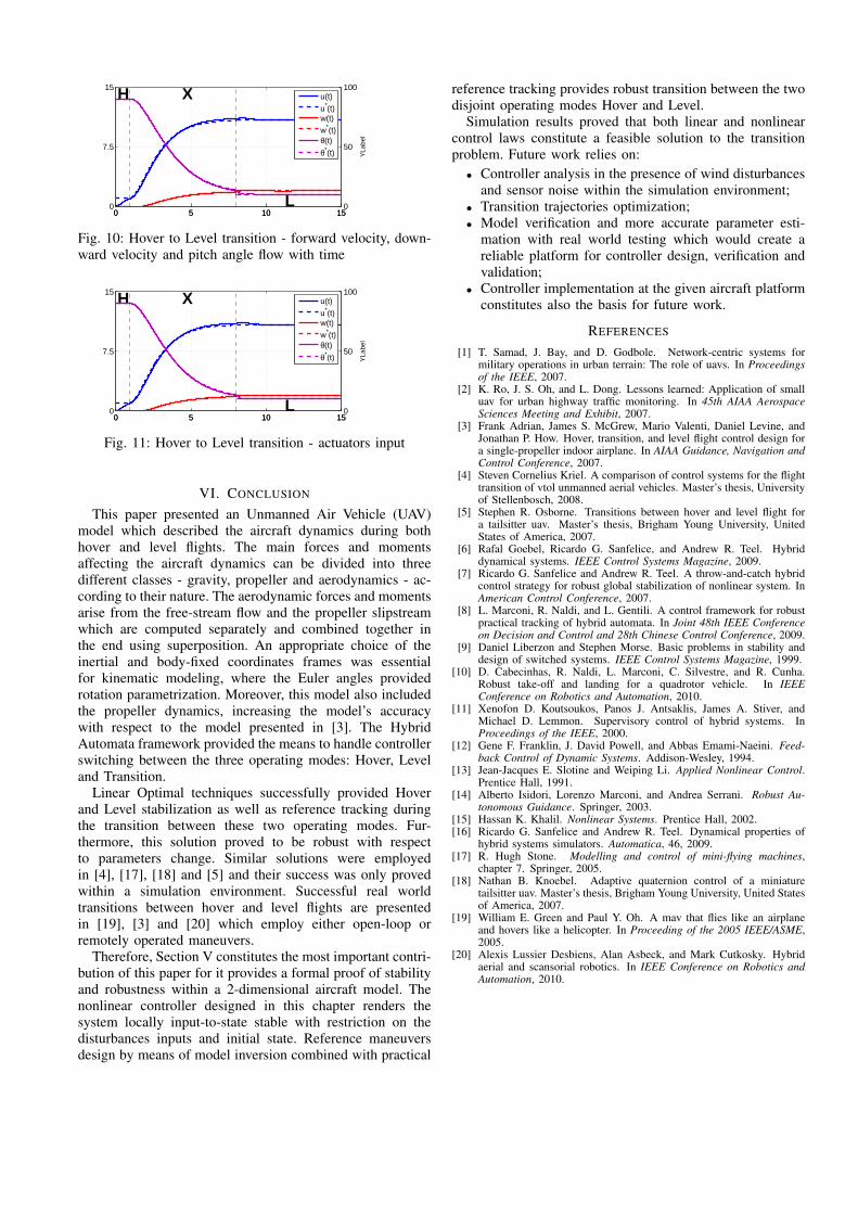
Figure 10 depicts the aircraft state variables flow with timeand Figure 11. The aircraft starts in hover at u = 0 m/sand the local controller increases thrust in order to achievea forward velocity of u = 1 m/s which is the transitionmaneuver starting point. When the aircraft state is nearv?X→H(0) a switch occurs (at t ' 0.91 s) and the nonlinearcontroller is used in order to follow the reference. Transitionto level flight occurs when θ < θX→L (at t = 8.0 s) and thelocal regulator stabilizes the aircraft at the equilibrium point.

0 5 10 150

7.5

15 H X

L

0 5 10 150

50

100

YLa

bel

u(t)

u*(t)w(t)

w*(t)θ(t)

θ*(t)

Fig. 10: Hover to Level transition - forward velocity, down-ward velocity and pitch angle flow with time

0 5 10 150

7.5

15 H X

L

0 5 10 150

50

100

YLa

bel

u(t)

u*(t)w(t)

w*(t)θ(t)

θ*(t)

Fig. 11: Hover to Level transition - actuators input

VI. CONCLUSION

This paper presented an Unmanned Air Vehicle (UAV)model which described the aircraft dynamics during bothhover and level flights. The main forces and momentsaffecting the aircraft dynamics can be divided into threedifferent classes - gravity, propeller and aerodynamics - ac-cording to their nature. The aerodynamic forces and momentsarise from the free-stream flow and the propeller slipstreamwhich are computed separately and combined together inthe end using superposition. An appropriate choice of theinertial and body-fixed coordinates frames was essentialfor kinematic modeling, where the Euler angles providedrotation parametrization. Moreover, this model also includedthe propeller dynamics, increasing the model’s accuracywith respect to the model presented in [3]. The HybridAutomata framework provided the means to handle controllerswitching between the three operating modes: Hover, Leveland Transition.

Linear Optimal techniques successfully provided Hoverand Level stabilization as well as reference tracking duringthe transition between these two operating modes. Fur-thermore, this solution proved to be robust with respectto parameters change. Similar solutions were employedin [4], [17], [18] and [5] and their success was only provedwithin a simulation environment. Successful real worldtransitions between hover and level flights are presentedin [19], [3] and [20] which employ either open-loop orremotely operated maneuvers.

Therefore, Section V constitutes the most important contri-bution of this paper for it provides a formal proof of stabilityand robustness within a 2-dimensional aircraft model. Thenonlinear controller designed in this chapter renders thesystem locally input-to-state stable with restriction on thedisturbances inputs and initial state. Reference maneuversdesign by means of model inversion combined with practical

reference tracking provides robust transition between the twodisjoint operating modes Hover and Level.

Simulation results proved that both linear and nonlinearcontrol laws constitute a feasible solution to the transitionproblem. Future work relies on:• Controller analysis in the presence of wind disturbances

and sensor noise within the simulation environment;• Transition trajectories optimization;• Model verification and more accurate parameter esti-

mation with real world testing which would create areliable platform for controller design, verification andvalidation;

• Controller implementation at the given aircraft platformconstitutes also the basis for future work.

REFERENCES

[1] T. Samad, J. Bay, and D. Godbole. Network-centric systems formilitary operations in urban terrain: The role of uavs. In Proceedingsof the IEEE, 2007.

[2] K. Ro, J. S. Oh, and L. Dong. Lessons learned: Application of smalluav for urban highway traffic monitoring. In 45th AIAA AerospaceSciences Meeting and Exhibit, 2007.

[3] Frank Adrian, James S. McGrew, Mario Valenti, Daniel Levine, andJonathan P. How. Hover, transition, and level flight control design fora single-propeller indoor airplane. In AIAA Guidance, Navigation andControl Conference, 2007.

[4] Steven Cornelius Kriel. A comparison of control systems for the flighttransition of vtol unmanned aerial vehicles. Master’s thesis, Universityof Stellenbosch, 2008.

[5] Stephen R. Osborne. Transitions between hover and level flight fora tailsitter uav. Master’s thesis, Brigham Young University, UnitedStates of America, 2007.

[6] Rafal Goebel, Ricardo G. Sanfelice, and Andrew R. Teel. Hybriddynamical systems. IEEE Control Systems Magazine, 2009.

[7] Ricardo G. Sanfelice and Andrew R. Teel. A throw-and-catch hybridcontrol strategy for robust global stabilization of nonlinear system. InAmerican Control Conference, 2007.

[8] L. Marconi, R. Naldi, and L. Gentili. A control framework for robustpractical tracking of hybrid automata. In Joint 48th IEEE Conferenceon Decision and Control and 28th Chinese Control Conference, 2009.

[9] Daniel Liberzon and Stephen Morse. Basic problems in stability anddesign of switched systems. IEEE Control Systems Magazine, 1999.

[10] D. Cabecinhas, R. Naldi, L. Marconi, C. Silvestre, and R. Cunha.Robust take-off and landing for a quadrotor vehicle. In IEEEConference on Robotics and Automation, 2010.

[11] Xenofon D. Koutsoukos, Panos J. Antsaklis, James A. Stiver, andMichael D. Lemmon. Supervisory control of hybrid systems. InProceedings of the IEEE, 2000.

[12] Gene F. Franklin, J. David Powell, and Abbas Emami-Naeini. Feed-back Control of Dynamic Systems. Addison-Wesley, 1994.

[13] Jean-Jacques E. Slotine and Weiping Li. Applied Nonlinear Control.Prentice Hall, 1991.

[14] Alberto Isidori, Lorenzo Marconi, and Andrea Serrani. Robust Au-tonomous Guidance. Springer, 2003.

[15] Hassan K. Khalil. Nonlinear Systems. Prentice Hall, 2002.[16] Ricardo G. Sanfelice and Andrew R. Teel. Dynamical properties of

hybrid systems simulators. Automatica, 46, 2009.[17] R. Hugh Stone. Modelling and control of mini-flying machines,

chapter 7. Springer, 2005.[18] Nathan B. Knoebel. Adaptive quaternion control of a miniature

tailsitter uav. Master’s thesis, Brigham Young University, United Statesof America, 2007.

[19] William E. Green and Paul Y. Oh. A mav that flies like an airplaneand hovers like a helicopter. In Proceeding of the 2005 IEEE/ASME,2005.

[20] Alexis Lussier Desbiens, Alan Asbeck, and Mark Cutkosky. Hybridaerial and scansorial robotics. In IEEE Conference on Robotics andAutomation, 2010.