Autonomous Vertical Recovery

of Fixed Wing

Unmanned Aerial Vehicles

by

Trevor R. Smouter

A thesis

presented to the University of Waterloo

in fulfillment of the

thesis requirement for the degree of

Master of Applied Science

in

Electrical and Computer Engineering

Waterloo, Ontario, Canada, 2013

© Trevor R. Smouter 2013

ii

AUTHOR'S DECLARATION

I hereby declare that I am the sole author of this thesis. This is a true copy of the thesis, including any

required final revisions, as accepted by my examiners.

I understand that my thesis may be made electronically available to the public.

iii

Abstract

As unmanned aerial vehicles (UAVs) prevail in commercial and first responder applications, the need

for safer and more consistent recovery methods is growing. Standard aircraft landing manoeuvres are

only possible with a suitable runway which is often unavailable outside of military applications.

Alternative recovery approaches can be either contained within the aircraft, ie. parachute or be setup

on the ground ie. net landing. By integrating the recovery system into the vehicle, the flight

preparation can be streamlined due to the fact that setting up recovering devices is no longer required.

The goal of this thesis is to investigate the application of an autonomous vertical landing capability

for fixed wing UAVs using articulated motors to enter vertical flight. Using an experimental UAV

design, the dynamics of the problem were investigated using recorded flight data. Implementing a

decoupled control approach, the aircraft was stabilized to maintain a horizontal hover. Through the

characterized plant model that defines the vertical descent behaviour, a control topology was

developed and tested in simulation using an optimal control approach. The developed controller was

tested on the experimental UAV to verify the vertical landing performance. It was determined that

this approach was well suited to autonomous vertical recovery of a fixed wing UAV. In employing

this approach to UAV recovery, operators can easily operate in theatres where space for conventional

landing does not exist.

iv

Acknowledgements

I would like to sincerely thank my supervisor, Professor David Wang, who provided guidance

throughout my research activities, mentored me in the ways of grad school and generally taught me to

calm down a little. I would also like to thank my readers, Professor Glenn Heppler and Professor

Daniel Davison for their time and counsel.

I would like to thank my friends Steve Buchanan and Ryan Tuner for the assistance they provided me

during my research experiments.

Finally, I must thank my wife Sarah, without her none of this would have been possible.

v

Dedication

This thesis is dedicated to my family:

First and foremost it is dedicated to my wife Sarah and our children Jacob and James. Without their

steadfast love, support, encouragement and understanding my education would not have been

possible.

To my mother, Annette, who cultivated my intelligence, inspired me to always reach higher and who

navigated my early education with a steady hand.

Also to my father Robert, whose technical abilities, strong work ethic and discipline have set the

example and made me the engineer I am today.

vi

Table of Contents

AUTHOR'S DECLARATION ...........................................................................................................ii

Abstract ........................................................................................................................................... iii

Acknowledgements .......................................................................................................................... iv

Dedication ......................................................................................................................................... v

Table of Contents ............................................................................................................................. vi

List of Figures ................................................................................................................................. vii

List of Tables ................................................................................................................................... ix

Chapter 1 Introduction ....................................................................................................................... 1

Chapter 2 Background ....................................................................................................................... 6

2.1 Modeling and Control of Altitude ............................................................................................ 9

2.2 Stability and Control .............................................................................................................. 12

Chapter 3 Experimental Design ....................................................................................................... 14

3.1 Experimental Airframe Development ..................................................................................... 17

3.2 Control Experiment and Data Systems ................................................................................... 21

3.3 General Dynamic Equations and Decoupling Controller ......................................................... 22

3.4 Combined Actuator Characterization...................................................................................... 24

3.5 Defining the Mixing Controller .............................................................................................. 28

3.6 Altitude Control Trim Identification ....................................................................................... 34

3.7 Airframe Stabilization ............................................................................................................ 36

Chapter 4 Altitude Control .............................................................................................................. 41

4.1 Altitude Measurement ............................................................................................................ 42

4.2 System Identification ............................................................................................................. 45

4.3 Controller Design................................................................................................................... 52

Chapter 5 Results ............................................................................................................................ 57

Chapter 6 Conclusions ..................................................................................................................... 68

6.1 Future Research ..................................................................................................................... 70

vii

List of Figures

Figure 1: Insitu’s ScanEagle being caught by the SkyHook ............................................................... 3

Figure 2: Front view of the Lux with motors in vertical position ....................................................... 4

Figure 3: The Lux shown with motors in the forward flight and vertical landing positions ................ 4

Figure 4: Boeing Vertol VZ-2 tilt wing [6] ....................................................................................... 6

Figure 5: V-22 Osprey in transitional flight [6] .................................................................................. 7

Figure 6: Rolls Royce thrust measuring rig [8] .................................................................................. 8

Figure 7: Hawker Siddeley Harrier in VTOL mode [11] ................................................................... 8

Figure 8: Altitude trajectory of autonomous helicopter landing [13] ................................................ 10

Figure 9: Autonomous descent of a vision based autonomous helicopter [15] ................................. 11

Figure 10: Wind generated disturbances acting on the Lux due to a high angle of attack ................. 14

Figure 11: The Lux with small wind induced disturbances due to optimal orientation ..................... 15

Figure 12: Altitude controller containing mixing controller (M) ....................................................... 16

Figure 13: Front profile view of the Lux with motors in vertical orientation ..................................... 18

Figure 14: Side profile of the Lux indicating CG and lift distribution ............................................... 18

Figure 15: The Lux with main motors in forward flight mode .......................................................... 19

Figure 16: The Lux with main motors tilting forward to generate forward acceleration while

descending ...................................................................................................................................... 19

Figure 17: The Lux yaw control by articulating the main motors while descending .......................... 20

Figure 18: The body axes and angular velocities of the Lux defined................................................ 24

Figure 19: Top view of the Lux's rotor arrangement ........................................................................ 26

Figure 20: Applied thrust relative to the center of gravity ............................................................... 26

Figure 21: Longitudinally applied forces ........................................................................................ 27

Figure 22: Lux main motor thrust vs throttle setting ........................................................................ 29

Figure 23: Main motor and tail motor thrust versus throttle setting.................................................. 30

Figure 24: Generated torque versus throttle setting .......................................................................... 31

Figure 25: Torque versus throttle setting after applying scaling factor to main motors ..................... 32

Figure 26: Throttle setting versus battery voltage ............................................................................ 35

Figure 27: Rate mode configuration................................................................................................. 36

Figure 28: Orientation mode on the roll axis ................................................................................... 37

Figure 29: The Lux at a small roll angle to accelerate to the left. ..................................................... 38

viii

Figure 30: Articulated main motors for longitudinal thrust to overcome wind induced drag .............. 39

Figure 31: The Lux side profile showing the fin area responsible for positive yaw stiffness ............. 39

Figure 32: Pressure altitude drifting over time while UAV altitude is fixed ..................................... 43

Figure 33: Simulated descent experiment showing pressure altitude drift ........................................ 43

Figure 34: Sonar data showing the reception of false pings ............................................................. 44

Figure 35: Proportional control loop used to stabilize the system .................................................... 45

Figure 36: System identification experiment using pseudo-random excitation ................................. 46

Figure 37: System identification results .......................................................................................... 47

Figure 38: Measured and modeled first order response ..................................................................... 48

Figure 39: Comparison of results between actual and Kalman filtered altitude related states ............ 51

Figure 40: LQR controller applied to altitude control ...................................................................... 53

Figure 41: LQR controller test with R = 1 ....................................................................................... 55

Figure 42: LQR controller test with R = 5 ....................................................................................... 56

Figure 43: Disturbance effects after 30 seconds of flight due to induced drafts ................................ 57

Figure 44: Altitude control using a PD controller set to 150cm (P=0.2 D=0.1) ................................ 58

Figure 45: Altitude control using a PD controller set to 150cm (P=0.3 D=0.1) ................................ 59

Figure 46: Altitude control using an LQR controller set to 150cm (R = 20) ..................................... 60

Figure 47: Altitude control using an LQR controller set to 150cm (R = 10) ..................................... 60

Figure 48: Altitude step control using an LQR controller comparing actual to simulated (R = 5) ...... 61

Figure 49: The four stages of autonomous descent, 1 – constant descent using pressure altitude

reference, 2 – parabolic deceleration using sonar reference, 3 – descent through ground effect, 4 –

motor wind down after touchdown................................................................................................... 64

Figure 50: Controlled descent at 10cm/s for investigating ground effect ........................................... 66

Figure 51: Descent manoeuvre and landing ..................................................................................... 67

ix

List of Tables

Table 1: Stabilization approaches of each axis ................................................................................ 37

Table 2: Typical accuracies and resolutions for common UAV altitude sensors ............................... 42

1

Chapter 1

Introduction

For over the past 100 years of heavier-then-air manned flight, there has been a common aphorism

spoken among aviators – it is better to be on the ground wishing you were in the air then to be in the

air wishing you were on the ground. While it is a cautious statement that “take-off is optional but

landing is mandatory”, it does not belie the fact that crashing is also in certain terms a landing.

Difficulties are compounded when the landing of aircrafts do not have the benefit of a prepared

airfield as is commonplace in UAV (unmanned aerial vehicle) missions.

The current growth in UAV system technologies and their emerging civil and commercial

applications [1] has brought about many new applications where modern control theory is used as a

tool to increase the performance and capabilities of the vehicles in this rapidly growing field.

Applications for alternative recovery methods are as varied as the uses for small UAVs. Typical

commercial applications for small UAVs routinely include mapping, surveying and aerial

photography [2]. Accuas Inc., a Canadian company, often flies missions for clients to create 3D maps

of quarries, mines and waste management sites necessary for both monitoring these sites as well as

for future planning [2]. Also, Unmanned Systems Canada provides competitions for teams using

UAVs for wildfire management in addition to search and rescue operations [3]. Operating out of

these numerous areas provide challenges for recovery since the areas are most often unpredictable,

uneven and/or built up with brush. Conventional landing requires long gentle glide slopes to keep

low airspeed and low flight path angles. The old aviator’s adage that the probability of survival is

inversely related to the angle of arrival definitely applies.

Over the past decade, new electric propulsion system technologies for aircraft have reshaped model

aviation and concurrently changed the landscape of small UAV systems and applications. Electric

propulsion has led to the proliferation of a family of vertical take-off and landing (VTOL) UAVs

known as multi rotor aircraft, which rely on the high bandwidth response unique to electric

propulsion in order to achieve stability. While these aircraft benefit from their simplicity due to very

few moving parts as compared to other VTOL aircraft, ie. helicopters, they lack the efficiency and

range required for many UAV applications. The most common UAVs for military and commercial

applications remain the fixed wing aircraft due to their much higher efficiency and subsequently

longer range and longer duration missions. Small fixed wing UAVs also benefit from the new

electric propulsion technologies. The electric motor is nearly vibration free compared with the

2

alternative combustion engines, leading to better payload capabilities. For instance, electric

propulsion allows optical systems that are sensitive to vibration. Other benefits include the ability to

stop and start the motor in flight, cleaner operation and a much lower noise pollution. These features

foster operations which are more flexible, especially for commercial operators where missions are

most likely to be conducted in noise sensitive areas.

The rise of commercial applications for small UAVs and the growing acceptance of these activities by

their respective governing agencies have allowed UAV operations to push into areas where aviation

infrastructure, ie. runways, are often unavailable. Currently, the largest impediments to these

operations are UAV recovery which ultimately governs the mission success. If the UAV is damaged

during the recovery process, it most often means that operations must be temporarily suspended until

the necessary repairs can be completed. Much of the time take-off is not a problem as it can be easily

accomplished by hand-launch, slingshot or pneumatic catapult [4] depending on the size of the UAV.

Many mobile commercial UAVs are of a hand launch size. If an adequate prepared strip is

unavailable for standard landing recovery, as is often the case for commercial operators, then

common alternatives include net-landing or parachute recovery. Both of these options remain high

risk. Net landing risks occur where the pilot is required to manually fly the UAV into a net which is

of similar construction to a volley ball net. Clearly, this is a difficult task to execute in that it requires

a highly skilled pilot for the mission operation as well as excluding the option of autonomous landing.

Even if the net is hit squarely, there is a large possibility that the UAV will either flip forward over

the net or bounce back out, often landing on the tail and causing damage that suspends the mission

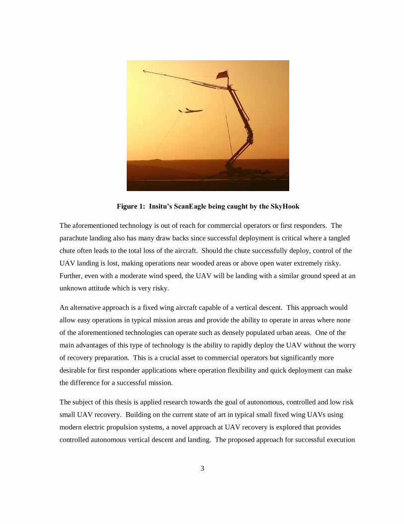
flights. While other recovery methods exist for these areas, such as trailered net landings or Institu’s

Scan Eagle recovery known as the skyhook (Figure 1), they require large trailers and are more suited

to their military applications.

3

Figure 1: Insitu’s ScanEagle being caught by the SkyHook

The aforementioned technology is out of reach for commercial operators or first responders. The

parachute landing also has many draw backs since successful deployment is critical where a tangled

chute often leads to the total loss of the aircraft. Should the chute successfully deploy, control of the

UAV landing is lost, making operations near wooded areas or above open water extremely risky.

Further, even with a moderate wind speed, the UAV will be landing with a similar ground speed at an

unknown attitude which is very risky.

An alternative approach is a fixed wing aircraft capable of a vertical descent. This approach would

allow easy operations in typical mission areas and provide the ability to operate in areas where none

of the aforementioned technologies can operate such as densely populated urban areas. One of the

main advantages of this type of technology is the ability to rapidly deploy the UAV without the worry

of recovery preparation. This is a crucial asset to commercial operators but significantly more

desirable for first responder applications where operation flexibility and quick deployment can make

the difference for a successful mission.

The subject of this thesis is applied research towards the goal of autonomous, controlled and low risk

small UAV recovery. Building on the current state of art in typical small fixed wing UAVs using

modern electric propulsion systems, a novel approach at UAV recovery is explored that provides

controlled autonomous vertical descent and landing. The proposed approach for successful execution

4

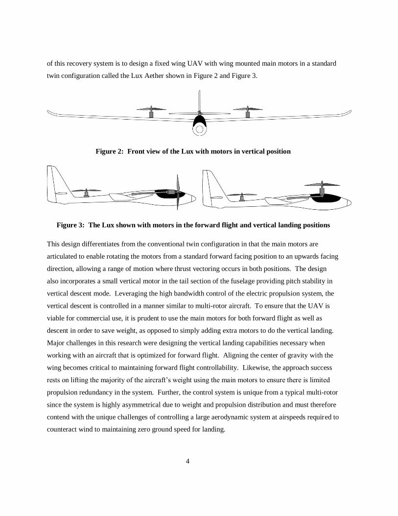
of this recovery system is to design a fixed wing UAV with wing mounted main motors in a standard

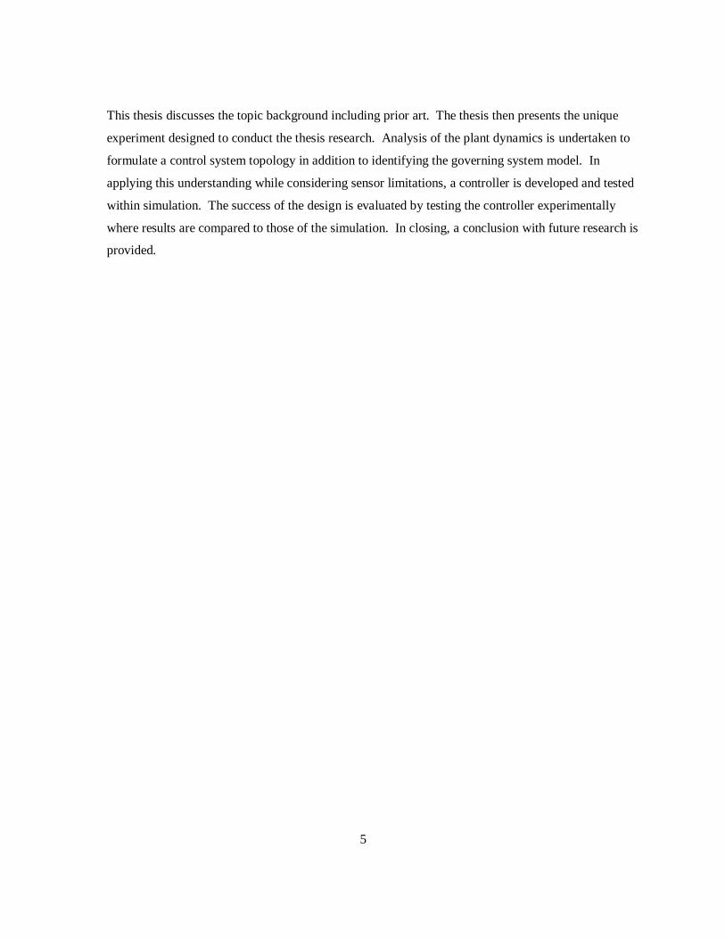
twin configuration called the Lux Aether shown in Figure 2 and Figure 3.

Figure 2: Front view of the Lux with motors in vertical position

Figure 3: The Lux shown with motors in the forward flight and vertical landing positions

This design differentiates from the conventional twin configuration in that the main motors are

articulated to enable rotating the motors from a standard forward facing position to an upwards facing

direction, allowing a range of motion where thrust vectoring occurs in both positions. The design

also incorporates a small vertical motor in the tail section of the fuselage providing pitch stability in

vertical descent mode. Leveraging the high bandwidth control of the electric propulsion system, the

vertical descent is controlled in a manner similar to multi-rotor aircraft. To ensure that the UAV is

viable for commercial use, it is prudent to use the main motors for both forward flight as well as

descent in order to save weight, as opposed to simply adding extra motors to do the vertical landing.

Major challenges in this research were designing the vertical landing capabilities necessary when

working with an aircraft that is optimized for forward flight. Aligning the center of gravity with the

wing becomes critical to maintaining forward flight controllability. Likewise, the approach success

rests on lifting the majority of the aircraft’s weight using the main motors to ensure there is limited

propulsion redundancy in the system. Further, the control system is unique from a typical multi-rotor

since the system is highly asymmetrical due to weight and propulsion distribution and must therefore

contend with the unique challenges of controlling a large aerodynamic system at airspeeds required to

counteract wind to maintaining zero ground speed for landing.

5

This thesis discusses the topic background including prior art. The thesis then presents the unique

experiment designed to conduct the thesis research. Analysis of the plant dynamics is undertaken to

formulate a control system topology in addition to identifying the governing system model. In

applying this understanding while considering sensor limitations, a controller is developed and tested

within simulation. The success of the design is evaluated by testing the controller experimentally

where results are compared to those of the simulation. In closing, a conclusion with future research is

provided.

6

Chapter 2

Background

Autonomous recovery of a fixed wing UAV using vertical flight hails from research into vertical

take-off and landing (VTOL) aircraft, although this application is focused only on the landing portion

of the technology. The first recorded evidence of humans contemplating heavier than air VTOLs

similar to helicopters we know today was Leonardo da Vinci’s helicopter drawings from 1493 [5].

Approximately 450 years later, early rotary wing helicopter prototypes would take to the air in leaps

and bounds. While the roots of fixed wing aircraft technologies can be easily traced to its respective

inventors, the helicopter has a more muddied history with many inventors [6]. The modern helicopter

design we know today is largely attributed to Igor Sikorsky and consisted of a main lifting rotor with

cyclic controls for pitch and roll control with a sideward thrusting tail rotor for anti-torque and yaw

control [6]. With production versions appearing in 1941, applications for the reliable VTOL aircraft

were military focused. The ability of the helicopter to take off and land without a prepared runway

was an advantage for military applications like giving the ability to drop troops in conflict areas.

To overcome the inefficiencies of rotary wing flight while maintaining the launch and recovery

benefits afforded by VTOL, starting in the 1950’s, aircraft manufacturers perused hybrid designs

known as tilt-wing and tilt-rotor designs [7]. While helicopters are more mechanically complex than

airplanes, tilt wing/rotor aircraft are significantly more complex than helicopters. The tilt wing

design had wing mounted engines that would articulate vertically by rotating the entire wing (a type

of which is depicted in Figure 4).

Figure 4: Boeing Vertol VZ-2 tilt wing [6]

7

Each rotor still maintains the complexity required of a helicopter rotor to conduct hovering flight [7].

The designs were difficult to pilot during the transitions from each mode of flight and while many

manufacturers made prototype tilt wing designs, they have never been put into production [6]. The

tilt rotor concept differs in that the rotors are mounted at the ends of the wing and only the rotors tilt

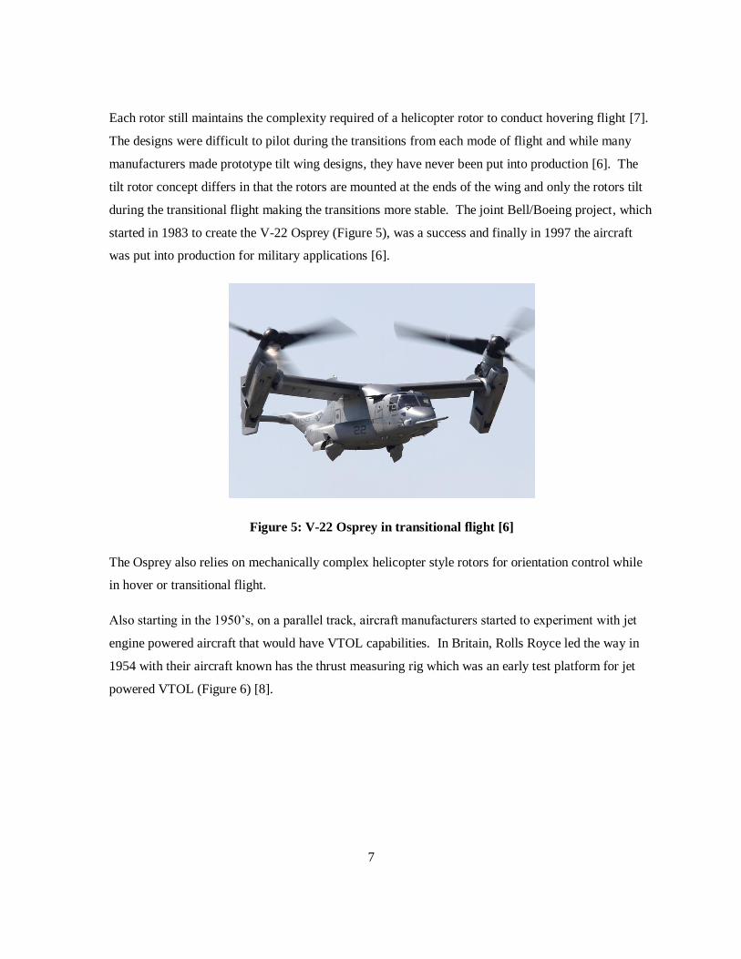
during the transitional flight making the transitions more stable. The joint Bell/Boeing project, which

started in 1983 to create the V-22 Osprey (Figure 5), was a success and finally in 1997 the aircraft

was put into production for military applications [6].

Figure 5: V-22 Osprey in transitional flight [6]

The Osprey also relies on mechanically complex helicopter style rotors for orientation control while

in hover or transitional flight.

Also starting in the 1950’s, on a parallel track, aircraft manufacturers started to experiment with jet

engine powered aircraft that would have VTOL capabilities. In Britain, Rolls Royce led the way in

1954 with their aircraft known has the thrust measuring rig which was an early test platform for jet

powered VTOL (Figure 6) [8].

8

Figure 6: Rolls Royce thrust measuring rig [8]

Rolls Royce eventually produced Britain’s first VTOL aircraft called the Short SC.1. The SC.1 used

four vertically mounted engines for VTOL and a larger engine for forward flight [9]. Developments

made on the SC.1 found their way through the experimental Hawker Siddeley P.1127 to the

production Hawker Siddeley Harrier (known colloquially as the Harrier Jump Jet) [10]. The Harrier

(Figure 7), uses thrust vectoring to generate lift in VTOL manoeuvres and a reaction control system

(RCS) which is made of strategically placed jets used to control orientation [10].

Figure 7: Hawker Siddeley Harrier in VTOL mode [11]

Both the Osprey and Harrier are successful VTOL production aircraft that eliminate the dependence

on undamaged runways for operational capability and enables operation from unprepared sites [9].

For military applications the advantages are clear.

9

2.1 Modeling and Control of Altitude

This section provides a background on models for rotor craft in modes relating to hovering and

landing. Note that investigation of general models for aerial vehicles is beyond the scope of this

thesis.

Much of the work in the area of autonomous hovering and landing has been completed on helicopter

style VTOL UAVs. Fabiani et al. have shown successful use of a simple altitude controller in

autonomous helicopters [12].

The system provides the option to use either a vertical velocity or altitude as a reference. The plant

model is defined as a first order transfer function of the helicopters collective control in series with a

first order transfer function that models the velocity response due to the collective control input. An

integrator is used to relate the altitude to the vertical velocity. The altitude reference is received from

a GPS; therefore autonomous landing would be difficult to achieve successfully due to absolute errors

in the measurement.

A more detailed approach to autonomous helicopter landing has been described by Seong-Pil Kim et

al. where the analysis was based on a helicopter with stable trimmed attitude [13]. The control law

presented was a 2 degree of freedom (DOF) tracking control law which was shown to be globally

stable using the Lyapunov stability theorem. While the paper specifically discusses autonomous

landing, the experiment presented stopped short of actual touchdown (Figure 8) and it was considered

future research.

10

Figure 8: Altitude trajectory of autonomous helicopter landing [13]

The application of a differential global positioning system (DGPS) for positional measurement

provided the required resolution to properly control the aircraft. Strategies for handling control into

the ground effect were absent from the methodology presented. The conclusion was that the

controller used for stable hover enables autonomous unmanned helicopter landing which had been

demonstrated in flight.

The aforementioned work was loosely based on a paper by J. Kaloust et al. that presented a nonlinear

controller for a 2-DOF helicopter model [14]. The work used Lyapunov’s direct method to establish

stability and used a recursive design technique to generate a controller. The method developed an

approach that appropriately handles the nonlinearity experienced with large control inputs to the

helicopters collective control.

Autonomous helicopter landing conducted by Saripalli et al. investigates vision based position control

to hold the helicopter over the landing site [15]. The work includes no indication of what the circuit

height altitude measurement device is; however, it does mention that an ultrasonic sensor is used near

the ground. The autopilot altitude control has three modes called hover control, velocity control and

sonar control. Target location is conducted under hover control and once centered over the target, the

velocity control is enabled to conduct the descent. Once the sonar measurements are reliable enough,

the autopilot switches to sonar control. The work shows the velocity and sonar controllers to be

11

simple PI controllers. The autonomous descent shown in Figure 9 shows a descent rate of 20cm/s

after the landing target has been identified.

Figure 9: Autonomous descent of a vision based autonomous helicopter [15]

An altitude controller designed specifically for a four rotor flying robot is presented by D. Gurdan et

al. that compensates for the altitude trim offset as the battery loses power [16]. The design describes

using two controllers; one is based on the use of an accumulator that essentially acts as an integrator

to slowly compensate for changes in the battery condition that will affect the neutral buoyancy

throttle position. The second controller is capable of fast responses ideal for disturbance rejection and

is implemented as a PD loop. The complete system is essentially a PID controller. The altitude

feedback for this multi-rotor is received from an external motion tracking vision system.

All of the altitude models and control systems discussed in this section also rely on a stability control

system used to maintain the aircrafts level orientation during descent. The next section discusses

approaches used to achieve this required stability.

12

2.2 Stability and Control

A control system is also required to maintain the orientation and stability of a hovering aircraft in

flight. This section describes background of some of the various approaches used to achieve this

stability.

The approach to stabilization of a four rotor flying robot presented by D. Gurdan et al. uses a model

free approach that requires tuning to achieve the desired performance [16]. The approach is unique in

that it integrates the sum of the control input and gyro feedback. Integrating only the gyro feedback

provides an orientation estimation that is subject to gyro drift and external disturbances. Their

approach sums the control input to the gyro feedback before integrating to generate an orientation

estimate that compensates for the drift. The overall control system would be considered a PID

controller.

In the work of S. Bouabdallah et al., an approach to quad-rotor stabilization control is developed

using a full Euler-Lagrange determined model of the system [17]. Investigation into system control

using both a sliding-mode controller and back stepping controller were explored. It was found that

back stepping control provided superior results to the sliding-mode control implementation. Note that

these tests required the use of an external control computer communicating to the quad-rotor and that

all the tests were conducted on a test stand with 3 degrees of freedom.

Also, in the work of B. Erginger and E. Altug great effort is put into generating a quad-rotor model

[18]. However, the model was only used for simulation purposes and ultimately a PD controller was

used for the orientation control while in simulation.

There are varied approaches that have been explored and tested in regards to VTOL aircraft

stabilization. While it is clear there has been some advanced work in defining the system dynamics to

generate realistic models, the control strategies seldom use a model based approach for control.

While a range of processors have been applied to the control of these systems, it is clear that

processing capability is a barrier to employing more advanced control schemes in flight. For practical

UAV applications high speed processing increases weight and consumes more power which affects

the aircrafts endurance rating. Also, ground based computing introduces latency into the control

system which reduces control system bandwidth and has significant reliability implications due to the

13

nature of radio links. For practical implementation of UAV technologies on board computing and

sensing is ideal and this requires implementation of effective and efficient control strategies.

14

Chapter 3

Experimental Design

Autonomous fixed-wing UAV recovery, the subject of this thesis, is predicated on electric propulsion

to maintain controlled orientation and descent of the aircraft. The controlled descent of such an

aerodynamic body diverges significantly from standard multi-rotor control by the necessity to

conduct these manoeuvres far outside the intended operational envelope of the airframe. The control

effort required to successfully complete an autonomous descent and landing can be studied in two

parts. First would be the control of the orientation of the aircraft and second, the control of the aircraft

translation in space relative to an inertial frame. For standard multi-rotor or helicopter control,

orientation is used to directly control translational motion since the thrust vector is approximately

fixed to the vertical axis of the aircraft’s body frame. For vertical descent fixed-wing UAV recovery

this topology leads to control difficulties related to disturbances generated by the aircraft’s lift

generating surfaces. The autonomous landing manoeuver requires that the aircraft counteract wind

speed during the descent so that at the moment of touchdown there is zero ground speed. The natural

consequence of this requirement is motion in the wind frame that acts on the lift generating surfaces

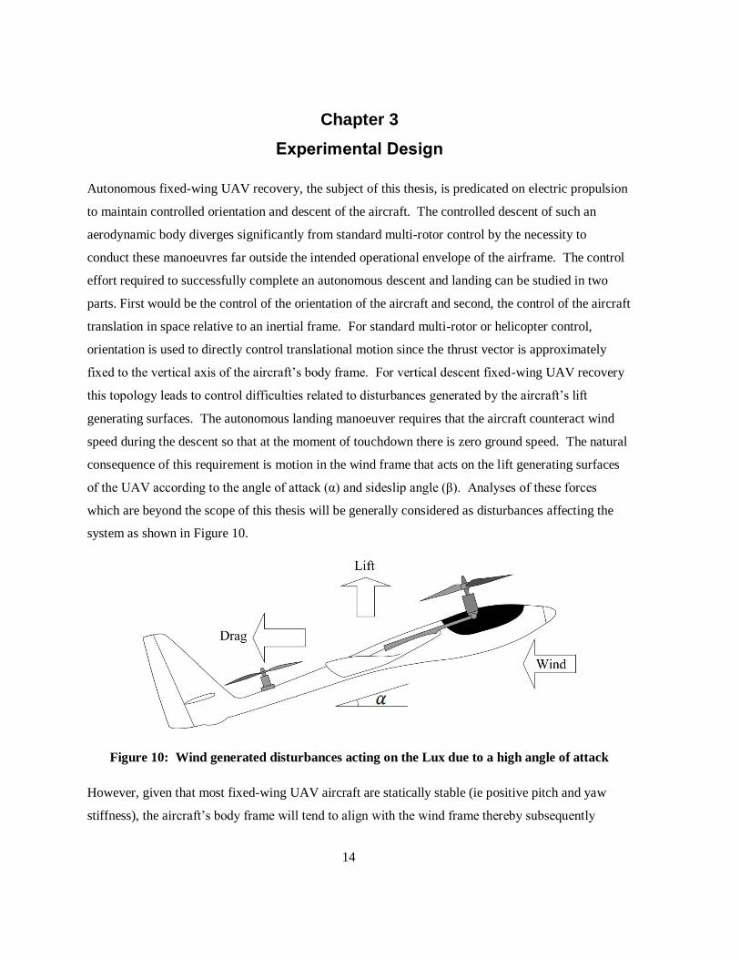
of the UAV according to the angle of attack (α) and sideslip angle (β). Analyses of these forces

which are beyond the scope of this thesis will be generally considered as disturbances affecting the

system as shown in Figure 10.

Figure 10: Wind generated disturbances acting on the Lux due to a high angle of attack

However, given that most fixed-wing UAV aircraft are statically stable (ie positive pitch and yaw

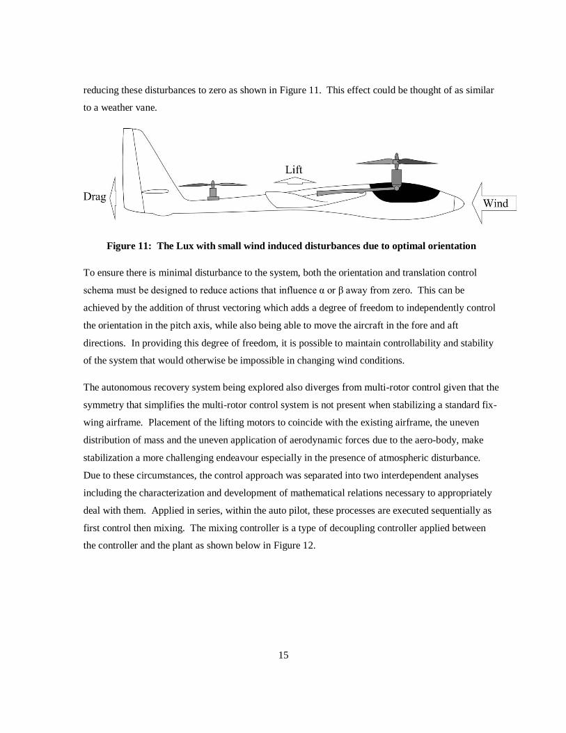
stiffness), the aircraft’s body frame will tend to align with the wind frame thereby subsequently

15

reducing these disturbances to zero as shown in Figure 11. This effect could be thought of as similar

to a weather vane.

Figure 11: The Lux with small wind induced disturbances due to optimal orientation

To ensure there is minimal disturbance to the system, both the orientation and translation control

schema must be designed to reduce actions that influence α or β away from zero. This can be

achieved by the addition of thrust vectoring which adds a degree of freedom to independently control

the orientation in the pitch axis, while also being able to move the aircraft in the fore and aft

directions. In providing this degree of freedom, it is possible to maintain controllability and stability

of the system that would otherwise be impossible in changing wind conditions.

The autonomous recovery system being explored also diverges from multi-rotor control given that the

symmetry that simplifies the multi-rotor control system is not present when stabilizing a standard fix-

wing airframe. Placement of the lifting motors to coincide with the existing airframe, the uneven

distribution of mass and the uneven application of aerodynamic forces due to the aero-body, make

stabilization a more challenging endeavour especially in the presence of atmospheric disturbance.

Due to these circumstances, the control approach was separated into two interdependent analyses

including the characterization and development of mathematical relations necessary to appropriately

deal with them. Applied in series, within the auto pilot, these processes are executed sequentially as

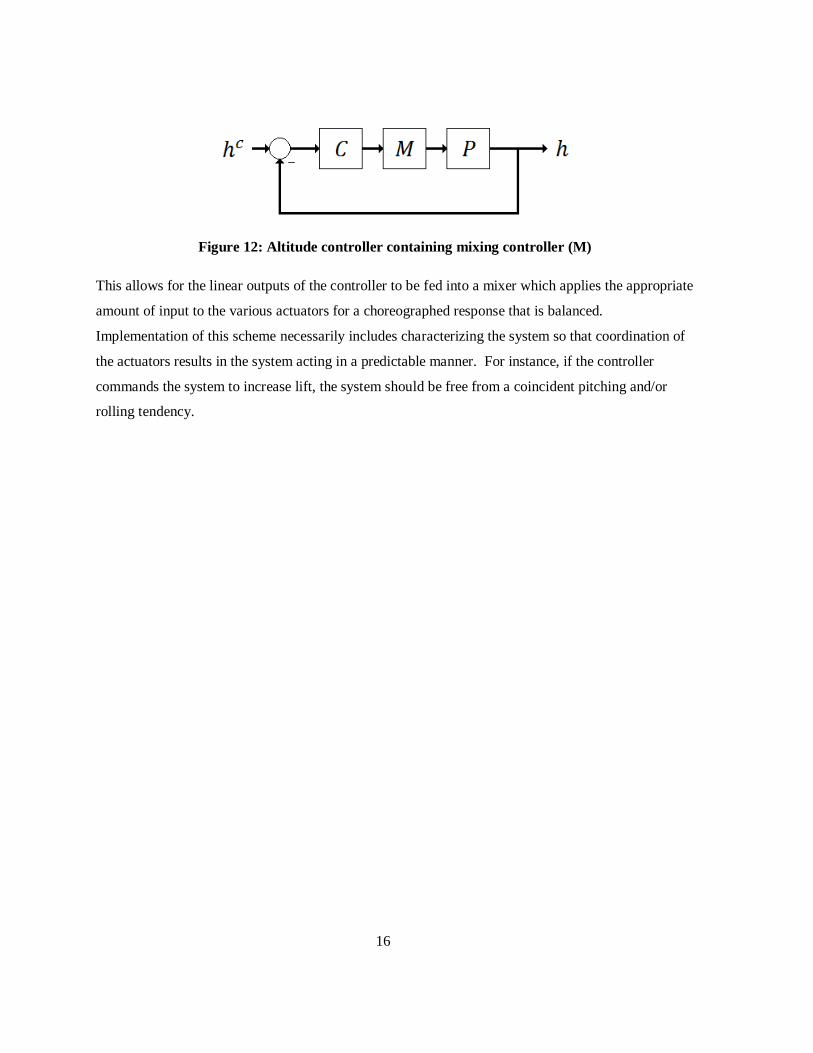
first control then mixing. The mixing controller is a type of decoupling controller applied between

the controller and the plant as shown below in Figure 12.

16

Figure 12: Altitude controller containing mixing controller (M)

This allows for the linear outputs of the controller to be fed into a mixer which applies the appropriate

amount of input to the various actuators for a choreographed response that is balanced.

Implementation of this scheme necessarily includes characterizing the system so that coordination of

the actuators results in the system acting in a predictable manner. For instance, if the controller

commands the system to increase lift, the system should be free from a coincident pitching and/or

rolling tendency.

17

3.1 Experimental Airframe Development

In order to study the control aspects of autonomous recovery, an experimental aircraft was required

that could facilitate the necessary data gathering experiments as well as test control hypotheses

developed throughout the research process. To ensure that the research could eventually be applied to

solving real world UAV recovery problems, it was prudent to experiment with typical UAV airframe

topologies. Before implementation, the focus of airframe procurement was directed at using a

sailplane style aircraft to modify for research purposes. Given that sailplanes have very high lift to

drag ratios, they are often chosen as commercial UAV platforms for their high efficiency such as the

CropCam UAV manufactured by MicroPilot [19].

A sailplane airframe made of Elapor foam was chosen as an experimental platform due to the fact that

it would hold up to various levels of abuse given the durability of Elapor compared with airframes

made of more rigid construction such as thin fiberglass shells. During the initial design phases mock-

ups were used to test weight distribution and to find a configuration that would likely accommodate

both the forward flight mode as well as the vertical descent. Once the proposed airframe topology

was decided upon, the two main motors and tail motor were built upon a simple wood test frame that

contained all the control devices including motor tilt actuators, electronic speed controllers, radio

receiver, microcontroller based autopilot, inertial measurement unit (IMU) and lithium polymer

(LiPo) battery. This enabled separate testing of the electric propulsion system for validation prior to

integration with the airframe. Once the main electronic propulsion and control systems were tested,

the test frame and sailplane were temporarily merged to ensure the proposed topology would be

successful prior to designing and assembling the final airframe. This process was valuable for

qualitatively determining the effect of the airframe, aerofoils and motor mounts within the wash

developed by the motors being operated in their vertical position. While these effects are outside the

scope of the thesis research, it was important to ensure the work done by the propulsion system was

effective enough to generate the required lift while the aircraft was in descent mode. Positioning of

the main motors was designed to strike a balance between applying lift near the center of gravity

while ensuring the lift generating wash was somewhat unimpeded by the airframe components. This

decision ensures the majority of the work in descent mode is being done efficiently by the main

motors while the tail motor (which is dead weight in forward flight mode) is used mostly for pitch

attitude control. The front profile view of the Lux can be seen in Figure 13 and shows the lateral

position of the two main motors.

18

Figure 13: Front profile view of the Lux with motors in vertical orientation

The longitudinal position of the main and tail motors (in descent mode) can be seen below in Figure

14. In can also be seen in the figure where the prop wash of the main motors overlaps the leading

edge of the wing and the motor nacelle.

Figure 14: Side profile of the Lux indicating CG and lift distribution

Extensive testing to find the ideal position of the motors for UAV recovery was not conducted. The

decision was pragmatic and based on both the issues mentioned above relating to balancing the center

of gravity as well as structural considerations to mitigate the stress (such as wing twisting) of lifting

the aircrafts weight in descent mode. The articulated main motors enable the Lux to operate in both

vertical descent mode as well as forward flight mode as shown below in Figure 15.

19

Figure 15: The Lux with main motors in forward flight mode

The articulating motor mounts designed to allow the Lux to convert between forward flight mode and

vertical descent mode also provide the Lux with extra degrees of freedom for control. The Lux

required the capability of accelerating forward and backwards without the pitching action that leads

to instability that was discussed above. This problem was solved by employing the extra degree of

freedom on each main motor to enable thrust vectoring. With the motors in the vertical position, it is

possible to tilt them both fore (as shown in Figure 16) and aft which provides a mechanism for

translation both forward and backwards.

Figure 16: The Lux with main motors tilting forward to generate forward acceleration while

descending

As well, in descent mode the heading of the aircraft can be controlled by tilting the motors in opposite

directions as shown in Figure 17.

20

Figure 17: The Lux yaw control by articulating the main motors while descending

21

3.2 Control Experiment and Data Systems

To facilitate control research using the Lux, the aircraft was equipped with numerous sensors, control

inputs and a data collection system. To coordinate the control and navigation operations using the

available sensor data, the Lux was equipped with a custom twin processor autopilot. One processor,

known as the flight controller, is mainly dedicated to interpreting external control references from

either the navigation processor or the safety pilot, executing high bandwidth inner loop control using

the inertial measurement unit (IMU), completing the required combined actuator mixing and

generating the output signals. The other processor, the navigation processor, is responsible for

interpreting the rest of the sensor data, executing navigation control as well as sending data to the

ground station for collection. The Lux uses a suite of onboard sensors:

IMU : data gathered from this sensor includes the rotation rate information ( ) and

orientation information ( )

Ultrasonic range finder: provides distance above ground level (AGL)

Barometric altimeter: provides a measure of the pressure altitude

GPS : provides geo-referenced location information

Also, attached to the navigation processor is a data modem which is used to transmit pertinent data to

a ground station for the purpose of data collection.

22

3.3 General Dynamic Equations and Decoupling Controller

The general dynamic equations for the UAV are described by [20],

where represents the system states such as position, velocity, orientation and angular velocity,

represents the total forces and moments due to all the actuators, ( ) describes the inertial effects

and represents the gravitational, centripetal and wind induced drag forces applied to the body. In

recovery mode the system is in a trimmed hover position where is the value of the states

corresponding with the trimmed position and giving,

where at steady state, is applied strictly to overcome gravitational effects. In the steady hover

manoeuvre, disturbances to the system will be corrected by the control system simplifying 3.2,

We are then left with,

where,

And,

( ) ( ) (3.1)

( ) (3.2)

( ) (3.3)

( ) (3.4)

(3.5)

23

We can find, in general, a decoupling controller such that where M is

designed to decouple the system dynamics [21]. In reality, this may only be possible at low

frequencies and the higher frequencies that are not decoupled would be considered a disturbance that

we reject with our control strategy. Hence, the strategy in this thesis is to decouple the system into a

subsystem for orientation and a subsystem for altitude.

In general we don’t know ( ) or ( ) so we will determine M experimentally to accomplish this

decoupling. Henceforth, since M is essentially combining different actuator signals in order to

accomplish this decoupling, the decoupling process will be referred to as mixing. This mixing is the

topic of the next section.

(3.6)

( ) (3.7)

24

3.4 Combined Actuator Characterization

Prior to working with the control aspects of the thesis, effort was put into system characterization

required for mixing the output signals of the controller in order to decouple the system as described in

the previous section. The most important aspect of coordinated actuator control was applying the

correct throttle signals to the different motors to affect balanced lift. Applying the throttle signal

alone must allow the Lux to generate lift that does not affect pitch or roll. The Lux’s body axes

and are defined in Figure 18 where , and are angular velocities and L, M and N are

applied moments in the roll, pitch and yaw directions respectively.

Figure 18: The body axes and angular velocities of the Lux defined

For a rigid body the inertia matrix is [22],

[ ∫( ) ∫ ∫

∫ ∫( ) ∫

∫ ∫ ∫( ) ]

[

] (3.8)

25

Since the Lux is built from a typical airplane configuration and the position of the motors maintain

the standard aircraft lateral symmetry on the plane spanned by and we have .

Then the moments of inertia matrix for the Lux is [23],

[

] (3.9)

Given the inertia matrix it can be shown that the rigid body equations of motion are [24],

( )

( ) ( )

( )

(3.10)

where , and are respectively the rolling, pitching and yawing moments due to . The rigid

body equations define a system that has some longitudinal and lateral coupling. However, it has been

shown that autopilots designed on the assumption of decoupled dynamics yield good performance

[23]. We may therefore make the simplification at this time and present the system when the axes are

principle [22],

( )

( )

( )

(3.11)

The externally applied moments about the axes and are represented by , and

respectively. In descent mode, when neglecting aerodynamic body forces, the main externally

applied moments are due to the rotor configuration. The rotor arrangement is shown below in Figure

19.

26

Figure 19: Top view of the Lux's rotor arrangement

This figure demonstrates that the main motors have lateral symmetry. Therefore a balanced

application of throttle to motors 1 and 2 results in no net moment input, . However, longitudinal

symmetry does not exist shown also in Figure 20 below.

Figure 20: Applied thrust relative to the center of gravity

27

The main concern is ensuring throttle changes do not affect the pitch attitude. The longitudinal forces

applied by the motors are shown in Figure 21.

Figure 21: Longitudinally applied forces

28

3.5 Defining the Mixing Controller

Noting Figure 21 in the previous section, the pitch moment is described by,

( ) (3.12)

The effect of the rotors thrust can be described by [23],

[( )

] (3.13)

Where is the air density, is the area swept by the prop, is the propellers lift coefficient,

is the airspeed incident on the propeller, is the throttle setting and is a gain that relates

the throttle setting to the airspeed leaving the prop. The control signal, , applied to the motor

controller is a pulse between 0 – 1000μs that relates to a motor RPM range. The value of is

defined by setting the pulse lengths that define both the minimum and maximum RPM to correspond

with the required propeller exit velocity airspeed.

In this application the forward speed of the prop in hover is negligible so 3.13 reduces to

( )

(3.14)

29

The thrust generated by the main motors was graphed (Figure 22) and indeed the throttle to thrust

relation is quadratic as shown on the trend line. However, it is also nearly linear over a generous

region around the operating point where the total generated thrust matches the weight of the vehicle.

Figure 22: Lux main motor thrust vs throttle setting

While not completely necessary, the throttle was linearized around the operating point as shown. To

balance the system, 3.15 and 3.16 were solved to find the trim position of each motor.

( ) (3.15)

(3.16)

Since is a programmable setting in the motor controller it can be adjusted to get the desired

throttle response from each motor controller. For balanced lift it is required that,

(3.17)

y = 0.0472x2 - 19.627x + 2043.8

y = 15.435x - 4453.8

0

500

1000

1500

2000

2500

3000

0 100 200 300 400 500

Thru

st (g

)

Throttle Setting (μs)

Measured

Modeled

Poly. (Measured)

Linear (Modeled)

30

By solving 3.17 for we have,

(3.18)

Then the system can be balanced by using the default value programmed into the motor controller for

to calculate the required . The motor controller for motor 3 is then programmed

with the appropriate value.

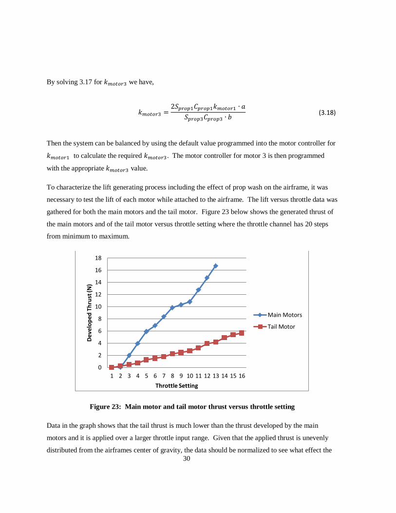
To characterize the lift generating process including the effect of prop wash on the airframe, it was

necessary to test the lift of each motor while attached to the airframe. The lift versus throttle data was

gathered for both the main motors and the tail motor. Figure 23 below shows the generated thrust of

the main motors and of the tail motor versus throttle setting where the throttle channel has 20 steps

from minimum to maximum.

Figure 23: Main motor and tail motor thrust versus throttle setting

Data in the graph shows that the tail thrust is much lower than the thrust developed by the main

motors and it is applied over a larger throttle input range. Given that the applied thrust is unevenly

distributed from the airframes center of gravity, the data should be normalized to see what effect the

0

2

4

6

8

10

12

14

16

18

1 2 3 4 5 6 7 8 9 10 11 12 13 14 15 16

Dev

elo

ped

Th

rust

(N)

Throttle Setting

Main Motors

Tail Motor

31

throttle will have on pitching the aircraft. Since the main motors apply thrust at point A as seen in

Figure 21, which is 16cm from the CG point and the tail motor applies thrust at point B which is

50cm from the CG point the applied torque can be obtained by multiplying the generated thrust by the

respective distance to the CG. Figure 24 shows the applied torque versus the throttle setting.

Figure 24: Generated torque versus throttle setting

These two applied torque data sets are reasonably matched and indicate the motors have been

appropriately sized for relative efficiency. To provide a balanced thrust during descent one of the

throttle signals will have to be scaled. By scaling the main motor throttle signal by 81.25% prior to

applying it to the front motors a more balanced throttle scheme is created as shown in Figure 25

below.

0

50

100

150

200

250

300

1 2 3 4 5 6 7 8 9 10 11 12 13 14 15 16

Torq

ue

(N-c

m)

Throttle Setting

Main Motors

Tail Motor

32

Figure 25: Torque versus throttle setting after applying scaling factor to main motors

One objective in the control scheme, to be discussed later, is to keep the aircraft pitch angle ( )

approximately zero to minimize the effect of velocity in the wind frame by keeping the angle of

attack near zero. While is near zero, controller outputs to correct pitch (applied differentially to the

main and tail motors) should be designed to not affect the total lift of the aircraft. To pitch the aircraft

forward the tail throttle should be increased and the main motor throttles should be decreased in such

a way that the total lift experienced by the aircraft remains constant. By comparing the thrust

generated by the different motors (Figure 25) it can be seen that the thrust generated by the tail motor

is approximately 30% of the main motor thrust across the calibrated throttle range. To prevent a net

change of lift during the application of a pitch command the signal applied to the main motors must

be -30% of that which is applied to the tail motor. Due to lateral symmetry, positioning commands

around the roll axis ( ) using the two main motors will not lead to a net change in the lift when is

approximately zero.

The success of the combined actuator characterization process was easily gauged by implementing

the mixing within the autopilot. The autopilot was set into a manual mode that allows commands

from a human safety pilot to control the aircraft via a radio transmitter. By hovering the Lux under

manual control, it was clear that the mixing scheme was working. However, given that the hover is

only operating the system within a very narrow throttle setting and the pilot has the ability to trim the

aircraft at that throttle setting a secondary test was conducted to confirm the proper mixing was be

-50

0

50

100

150

200

250

300

0 50 100 150 200

Torq

ue

(N-c

m)

Throttle Setting

Main Motors

Tail Motor

33

executed. The safety pilot was instructed to aggressively punch the throttle momentarily to see the

reaction of the aircraft. Repeated tests demonstrated the Lux jumping straight up from the hover

position without any pitch or roll tendencies’ confirming the mixing strategies was working

successfully.

Given that the Lux was built while carefully maintaining the CG at the position required for forward

flight, there was very little doubt about whether the aircraft would be able to successfully achieve

stable forward flight. Manual control flight tests with the motors in the forward flight positions

confirmed the aircraft was stable and graceful in this mode of flight and exhibited no negative

tendencies while flying. With the airframe fully tested and the actuator mixing working, the

investigations and experimentation into autonomous recovery could now be initiated by further plant

identification considering the aircraft response through the combined actuator control as a whole.

34

3.6 Altitude Control Trim Identification

In aircraft control systems, the trim position is the controller output when all the steady state errors

are zero. For altitude control it is the throttle setting where the aircraft is neutrally buoyant.

Compared with a proportional integral derivative (PID) control scheme, the trim position would be

the output of the integrator when there is zero steady state error. With the altitude control of the Lux,

it is desirable to know the throttle position that provides a steady unaccelerated hover to add the

control effort to. Without knowing the proper trim or neutral throttle setting, the altitude error signal

would have to get necessarily large before the aircraft could maintain a steady hover. To solve this

problem with the addition of an integrator would not be appropriate for this application. As soon as

the aircraft enters descent mode the controller requires the ability to stabilize the system without

waiting for the integrator to settle to the trimmed position.

Using the data modem, it is possible to record the throttle values in flight and determine the throttle

setting that provides a steady hover. The problem with this approach is that the throttle position for a

steady hover changes during the flight according to the condition of the battery. As the battery charge

is depleted the voltage starts to drop, this lower voltage requires a higher throttle setting applied to the

motor controller to maintain motor RPM.

To solve the trim issue, the aircraft was strapped down to a lift indicating test platform and operated

until the fully charged battery had been completely discharged. The battery voltage and throttle

setting was recorded while the aircraft throttle was adjusted to maintain neutral buoyancy as indicated

by the test stand. This test was completed five times and the results were aggregated to generate a

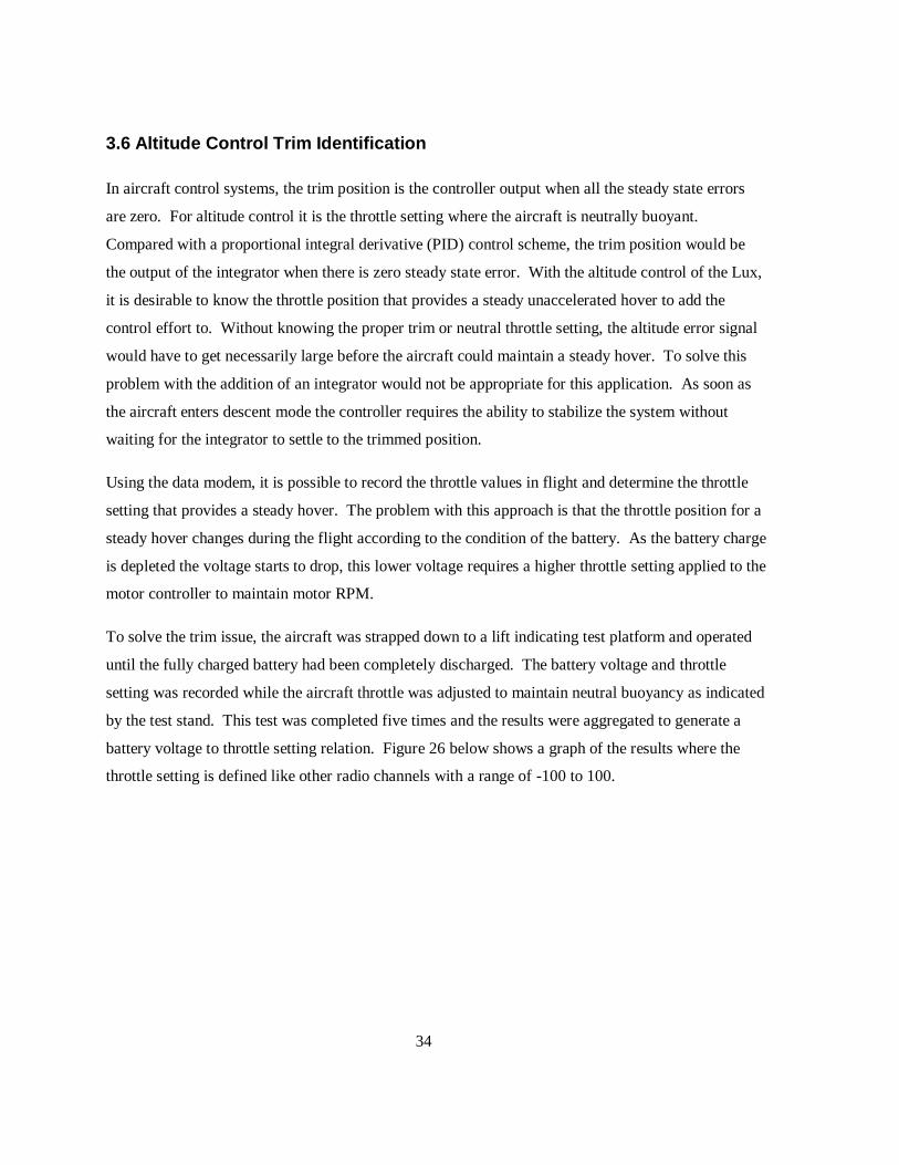
battery voltage to throttle setting relation. Figure 26 below shows a graph of the results where the

throttle setting is defined like other radio channels with a range of -100 to 100.

35

Figure 26: Throttle setting versus battery voltage

The trend line was used to generate the trim relationship. While the controller is operating in descent

mode the battery voltage is continually sampled and the trim setting is updated to the output throttle

command. Equation X below shows the throttle relationship with implemented trim.

( ) (3.19)

The total throttle command is the sum of the trimmed position, plus the required control effort as

demanded by the linear controller.

y = -17.707x + 236.77

-50

-45

-40

-35

-30

-25

-20

-15

-10

-5

0

13.5 14 14.5 15 15.5 16

Thro

ttle

Se

ttin

g

Battery Voltage (V)

Series1

Linear (Series1)

36

3.7 Airframe Stabilization

While the Lux has built-in positive pitch, roll and yaw stiffness while in forward flight the vertical

descent mode is inherently unstable. In fact, the vertical descent mode is impossible for the safety

pilot to control without some added help from the autopilot. Rate mode is used to aid the manual

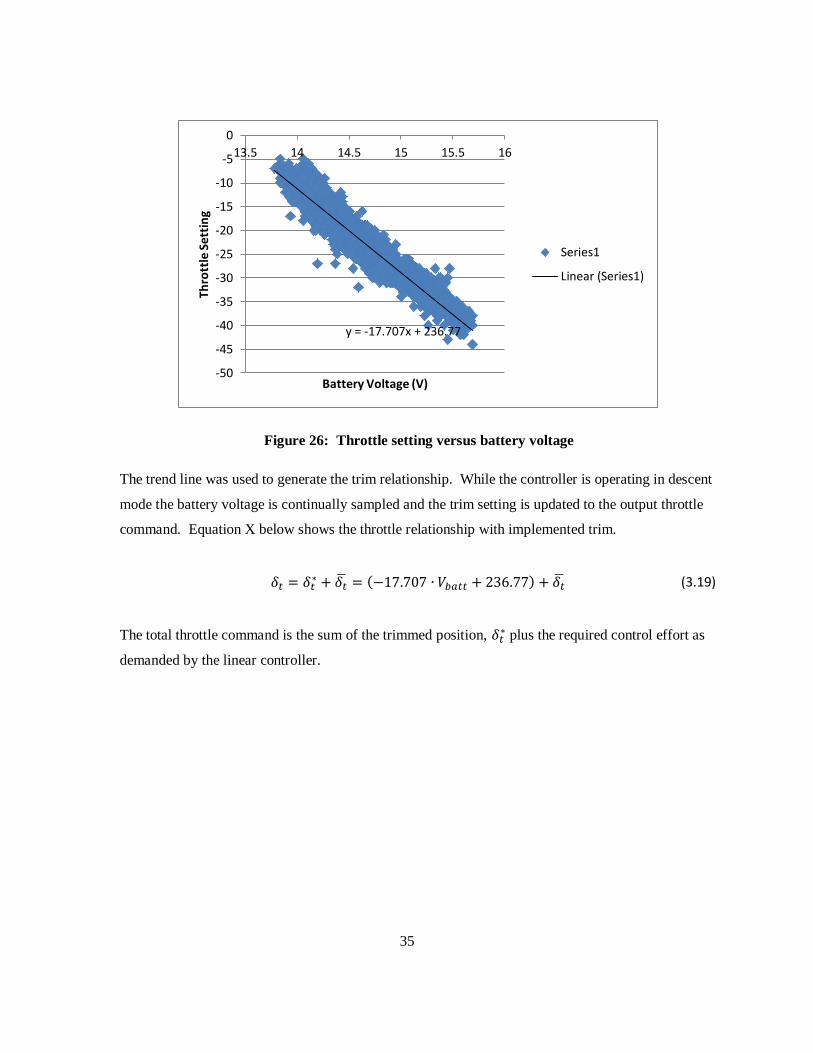
piloting control by adding damping to reduce the speed of the system. Figure 27 below shows the

basic rate mode configuration applied to the roll axis however both pitch and yaw axes have the same

topology.

Figure 27: Rate mode configuration

In Figure 27, is the roll angle, is the roll rate, is the roll command applied to the plant and

is the commanded roll rate. The plant is represented by the first order transfer function and the

integrator. The roll rate is conveniently available as an IMU gyro signal. The rate feedback is

multiplied by the derivative gain, and is then summed to the input signal provided by the pilot

control. The gain is easily tuned during flight testing by increasing gain until the system starts to

oscillate and then slightly backing off the gain until the oscillations stop. Note that the defined first

order plant in theory would not exhibit this tendency; however, higher order dynamics come into play

in practice. When properly tuned, the system counteracts external disturbances and requires more

input from the pilot to generate the desired manoeuvres. Increasing the input gain allows the pilot

control input to remain unaffected while still damping the system to any disturbances. Rate mode can

be used as a manual control autopilot safety override should the autonomous system react

unpredictably.

Orientation mode is built upon the rate mode topology. This mode can be used for autonomous flight

as well as manual control and differs from rate mode in that the control input is an orientation

command instead of a rate command. Figure 28 below shows the orientation mode configuration

applied to the roll axis.

37

Figure 28: Orientation mode on the roll axis

In this mode the roll position is sampled from the IMU and subtracted from the commanded roll

position to generate the error signal used to drive the inner rate loop discussed previously. The

outer orientation loop is tuned by increasing the proportional gain until the system holds an

upright orientation in flight without an external command signal. If is too large, oscillations are

likely to develop indicating that either or should be turned down.

Orientation mode is also ideal for manual override control in emergency situations. The pilot’s

control input will be different from rate mode which is analogous to a standard helicopter control in

that the stick positions map to axis orientations. Orientation mode benefits from the fact that if the

pilot assumes manual control and loses the attitude of the aircraft due to poor visibility or unusual

orientation simply releasing the control sticks will cause the aircraft to level out.

For the autonomous UAV recovery explored in this thesis, each axis is treated differently for

stabilization purposes. The stabilization approaches for each axis is summarized in Table 1 below.

Table 1: Stabilization approaches of each axis

Stabilization Mode Input Command Setting

Roll ( ) Orientation From navigation controller High

Pitch ( ) Orientation 0 degrees Medium

Yaw ( ) Rate 0 degrees/second Low

38

The differences in stabilization approach for each axis is based on both the control strategy as well as

the aircraft’s configuration in descent mode. The roll axis is configured for orientation mode

generally to maintain a level attitude during descent. If the landing scheme requires that the aircraft

land at a particular point or is required to avoid known obstacles during the descent, the lateral

direction of the aircraft can be influenced by the navigation controller by tilting the roll orientation as

shown below in Figure 29.

Figure 29: The Lux at a small roll angle to accelerate to the left.

Only a very small angle input for from the navigation controller is required to generate lateral

accelerations due to the small side profile of the Lux. Because the Lux’s long wings provide

significant rotational damping around the roll axis, a high gain is required to counteract the plants

mechanical damping when reacting to disturbances arising from unbalanced lift on the aerofoil.

As previously mentioned , in the presence of wind, angles of attack, , that deviate from zero have a

large undesirable influence on the altitude control stability. Therefore, to minimize this effect the

body frame and the wind frame is aligned by keeping the pitch angle close to zero. There is very

little mechanical damping on the pitch axis so must be high enough to damp out disturbances but

not too high that oscillations develop. As mentioned earlier, if it is desirable to counteract wind drift

in the longitudinal direction the main motors are articulated as shown in Figure 30 to provide the

required force to counteract wind induced drag.

39

Figure 30: Articulated main motors for longitudinal thrust to overcome wind induced drag

The yaw axis is unique in that this application calls for the allowance of the yaw angle to be

susceptible to external disturbances, specifically wind. The control strategy during autonomous

descent is designed around the Lux facing into the wind. Given the side profile shown in Figure 31,

the vertical stabilizer that provides positive yaw stiffness in forward flight is also effective at keeping

the lux facing into the wind during the descent manoeuver.

Figure 31: The Lux side profile showing the fin area responsible for positive yaw stiffness

By having the yaw axis in rate mode with an input of zero, the aircraft is damped in the yaw rotation

but is able to slowly weather vane into the wind during descent without employing other control

effort.

The application of the system decoupling and stabilization techniques provided in this chapter is

designed to keep the aircraft stable when in the vertical descent mode. Ultimately the control actions

keep the aircraft in an orientation designed to minimize the angle of attack and sideslip angle

which reduces aerodynamic forces that could destabilize the system if unaccounted for. This

hovering attitude allows the altitude to be controlled as if decoupled from the aircrafts orientation.

40

The analysis that follows in this thesis is predicated upon the controlled orientation described in this

chapter.

41

Chapter 4

Altitude Control

The focus of this thesis was handling the vertical descent control. In previous chapters, prerequisites

to the altitude control such as airframe design, actuator mixing and stabilization were discussed.

These items are critical to the system and once completed, define the system that will have its altitude

controlled for autonomous UAV recovery. To effectively control the aircrafts altitude in descent

mode is not a trivial matter for a couple reasons. The thrust required for descent is roughly five times

greater than what would be considered the maximum required for forward flight. In descent mode,

the majority of this thrust generated by the aircrafts propulsion system is used to support the weight of

the aircraft. Simply increasing the thrust required to achieve neutral buoyancy on the Lux by 1% (a

throttle resolution of 3 steps) induces a vertical velocity of approximately 60cm/s. This small input

generating large outputs is still reasonably controllable under ideal conditions but depends on good

quality data about the altitude state. System disturbances have considerable effects on the altitude

control which cannot be ignored. As noted, the aero-body generates significant forces under the

influence of wind. The thrust of the propellers is dependent on the propeller aerofoil angle of attack.

Changing winds affect this angle of attack leading to varying lift and increased altitude control

difficulty.

42

4.1 Altitude Measurement

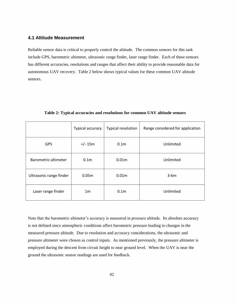
Reliable sensor data is critical to properly control the altitude. The common sensors for this task

include GPS, barometric altimeter, ultrasonic range finder, laser range finder. Each of these sensors

has different accuracies, resolutions and ranges that affect their ability to provide reasonable data for

autonomous UAV recovery. Table 2 below shows typical values for these common UAV altitude

sensors.

Table 2: Typical accuracies and resolutions for common UAV altitude sensors

Typical accuracy Typical resolution Range considered for application

GPS +/- 15m 0.1m Unlimited

Barometric altimeter 0.1m 0.01m Unlimited

Ultrasonic range finder 0.05m 0.01m 3-6m

Laser range finder 1m 0.1m Unlimited

Note that the barometric altimeter’s accuracy is measured in pressure altitude. Its absolute accuracy

is not defined since atmospheric conditions affect barometric pressure leading to changes in the

measured pressure altitude. Due to resolution and accuracy considerations, the ultrasonic and

pressure altimeter were chosen as control inputs. As mentioned previously, the pressure altimeter is

employed during the descent from circuit height to near ground level. When the UAV is near the

ground the ultrasonic sensor readings are used for feedback.

43

The barometric altimeter’s pressure altitude slowly drifts with changes in atmospheric conditions as

shown below in Figure 32.

Figure 32: Pressure altitude drifting over time while UAV altitude is fixed

To demonstrate the negligible effect of this drift the same data was overlaid upon a simulated descent

from 10m at a moderate descent rate of 40cm/s as shown in Figure 33 below.

Figure 33: Simulated descent experiment showing pressure altitude drift

This demonstrates that although the pressure altitude drifts over time, it is still possible to use the

barometric altimeter as decent measurement feedback device. Over the simulated descent using real

pressure data, the altitude error at the end was 37cm. Important is that this sensor is used during stage

0

20

40

60

80

100

120

140

0 20 40 60

alti

tud

e(c

m)

time (s)

Pressure Altitude

-200

0

200

400

600

800

1000

1200

0 10 20 30

alti

tud

e(cm

)

time (s)

Pressure Altitude

Actual Altitude

44

1 of the descent manoeuvre where the controller is controlling vertical velocity so sensor errors affect

the desired rate of descent. The drift in barometric pressure in the above simulation amounts to an

average measured descent rate of 41.48cm/s instead of the actual 40cm/s rate that was desired. This

small error is acceptable and is likely to be smaller than the effect of atmospheric disturbances

buffeting the aircraft.

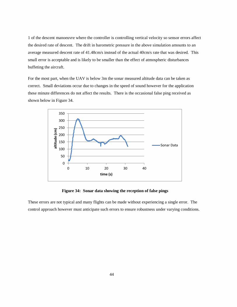
For the most part, when the UAV is below 3m the sonar measured altitude data can be taken as

correct. Small deviations occur due to changes in the speed of sound however for the application

these minute differences do not affect the results. There is the occasional false ping received as

shown below in Figure 34.

Figure 34: Sonar data showing the reception of false pings

These errors are not typical and many flights can be made without experiencing a single error. The

control approach however must anticipate such errors to ensure robustness under varying conditions.

0

50

100

150

200

250

300

350

0 10 20 30 40

alti

tud

e (c

m)

time (s)

Sonar Data

45

4.2 System Identification

Before attempting to characterize the plant, it was necessary to decide on the control objectives and

the control approach to meet those objectives. The two unique applications of altitude control during

autonomous recovery is the initial descent using the barometric altimeter as feedback and the landing

flare, where the aircraft is decelerated, using the ultrasonic rangefinder as feedback. These two stages

of the descent need to control the rate of descent and altitude AGL respectively. Therefore, the state

space system should track both the altitude and vertical velocity so that these states can be easily

monitored and controlled.

To define a simple system that tracks both vertical velocity and the altitude as states, it was desirable

to define the plant as a second order system including an integrator. Referring to 3.1 to 3.7 it is

expected that there would be one pole at the origin and the other pole would be a function of the

systems damping. This simplified system enables the use of modern control theory within the limited

processing capability of the autopilot. To characterize the system using a least squares identification

algorithm, it was necessary to first stabilize the system since open loop operation of the aircraft is

unstable. Employing a simple closed loop proportional controller prevents the aircraft from flying too

high or too low during the characterization process. The control loop is shown below in Figure 35

where is the altitude, is the vertical velocity, and is the commanded altitude.

Figure 35: Proportional control loop used to stabilize the system

The closed loop transfer function of this system is,

(4.1)

46

To identify the plant using Matlab, the system must be defined as a second order model with no zeros.

Using the identified transfer function, the second order plant model including the integrator, can be

extracted from the resultant system equation. In this case,

(4.2)

(4.3)

For this identification technique to work and provide the desired plant it is a necessity that .

If this requirement is not met then the second order transfer function including integrator will not be

the form identified. The system identification experiment was executed by exciting the system using

a pseudo random input as shown in Figure 36.

Figure 36: System identification experiment using pseudo-random excitation

The data was used to generate a transfer function that best fit the data as shown below in Figure 37.

The resulting transfer function received was,

-50

0

50

100

150

200

0 20 40 60 80 100 120 140

alti

tud

e (c

m)

time (s)

Altitude

Pseudo random input

47

(4.4)

For the system identification experiment , therefore if we assume the condition is

met we have,

(4.5)

(4.6)

Figure 37: System identification results

This would provide an internal transfer function of,

(4.7)

0 20 40 60 80 100 120-40

-30

-20

-10

0

10

20

30

40

Time

Measured and simulated model output

Model Response

Actual Response

48

Unfortunately, this transfer function provides a steady state gain of 3.47 where experimental evidence

gathered from fixing the throttle and measuring the corresponding steady state vertical velocity, has

shown that the actual gain of the system is approximately 20.

Seeking a more suitable model, a second approach was tested to characterize the system. The first

order response from throttle to vertical velocity was investigated through a series of experiments.

The aircraft was set to hover using a manually tuned PD controller. Once stabilized and settled, a

step input was provided to the throttle while recording the response of the altitude state. The typical

response can be seen in below Figure 38.

Figure 38: Measured and modeled first order response

After filtering and fitting the data the following transfer function was obtained.

(4.8)

Given the steady state gain for this transfer function is 21.5, these results are in agreement with earlier

tests that indicated the steady state gain was approximately 20. Interestingly, the pole location of this

identified plant is close to the pole location identified in the plant of 4.7.

Using the transfer function 4.8 and adding the integrator gives the plant model,

0

20

40

60

80

100

120

140

0 1 2 3 4

vert

ical

vel

oci

ty (c

m/s

)

time (s)

Model

Data

49

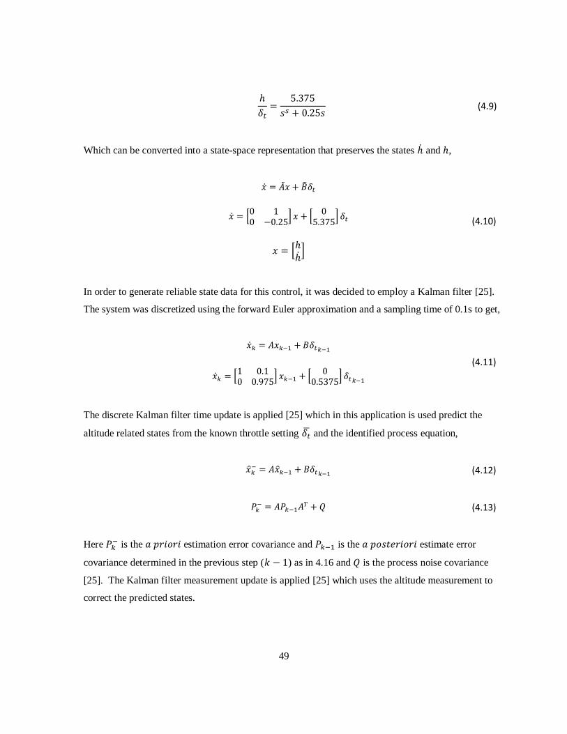
(4.9)

Which can be converted into a state-space representation that preserves the states and ,

[

] [

]

[ ]

(4.10)

In order to generate reliable state data for this control, it was decided to employ a Kalman filter [25].

The system was discretized using the forward Euler approximation and a sampling time of 0.1s to get,

[

] [

]

(4.11)

The discrete Kalman filter time update is applied [25] which in this application is used predict the

altitude related states from the known throttle setting and the identified process equation,

(4.12)

(4.13)

Here is the estimation error covariance and is the estimate error

covariance determined in the previous step ( ) as in 4.16 and is the process noise covariance

[25]. The Kalman filter measurement update is applied [25] which uses the altitude measurement to

correct the predicted states.

50

(

) (4.14)

(

) (4.15)

( ) (4.16)

The objective of the Kalman filter is to reduce the estimate error . In Equation 4.15

the residual, ( ) represents the difference between the measured and predicted states. The

value of calculated in 4.14 results in the minimizing of when applied to the residual in 4.15

[25].

The Kalman filter matrix equations were converted into a sequence of single line equations that could

be executed within the autopilots 16-bit microcontroller for in flight execution. Captured sensor data

was evaluated to determine the variance of the measured signals in order to generate the R matrix.

Note that since the system has two altitude measuring devices the R matrix needs to be changed

according to the sensor noise covariance of the particular sensor currently in use. In practical

applications, the determination of the Q matrix is difficult to determine and so the process noise ends

up being attributed mostly due to plant uncertainty [25]. Therefore, the Q matrix values were chosen

based on the results from simulations that were run using actual flight data. This was achieved by

adjusting the variance associated with the throttle to vertical velocity transfer function until the

estimate closely agreed with the measured data. Below in Figure 39, the comparison between the

actual and filtered data is displayed.

51

Figure 39: Comparison of results between actual and Kalman filtered altitude related states

The first half of the flight is stabilized using a simple manually tuned PD controller while the second

half is flight under safety pilot control. The flight shown uses the more accurate sonar for altitude

measurement so that the altitude state does not benefit from the filtering as much as the vertical

velocity state. The quality of the filtered vertical velocity compared with that which was derived

from the altitude measurement confirms the identified plant is a reasonable approximation.

30 35 40 45 50 55 60 65 70 75 80-100

-50

0

50

100

150

200

250

300altitude (

cm

), v

ert

ical velo

city (

cm

/s)

time(s)

actual altitude

estimated altitude

vertical velocity

estimated vertical velocity

52

4.3 Controller Design

In designing the controller, the system model was entered into simulation to develop and experiment

with a suitable altitude control scheme. Given the state feedback from the Kalman filter, a linear

quadratic regulator (LQR) controller seemed to be an ideal candidate for controlling the Lux’s

altitude. Note, this section of the thesis uses matrices and which are distinct from the

matrices presented in the previous section with Kalman filtering and are reused because they are

traditionally used when presenting an LQR control system. Since an LQR is an optimal control

system, it is designed to provide a minimum performance index where in this case the performance

index is,

where and , used to penalize the state vector and control signals, are positive semi definite and

positive definite respectively. In the plant model that is the subject of this thesis the two states being

tracked is the altitude and vertical velocity while the control input is the throttle . The choice

of Q and R can be defined as [24],

Where is the maximum desired altitude, is the maximum desired vertical velocity and

is the maximum desired throttle input [24].

The performance index in 4.17 is minimized when [26],

∫ (

)

(4.17)

[

]

(4.18)

53

Where, is a matrix which is found by solving the algebraic Riccati equation [26],

For the LQR used to control this system the control law is given by,

A block diagram of the system is shown below in Figure 40.

Figure 40: LQR controller applied to altitude control

Note that the state feedback shown is derived from the Kalman filter and can be shown to be optimal

according to the separation principle [26]. The complete system is now,

Since the control law has been defined, all that remains to be determined is the value to

appropriately turn the altitude command into a form that will properly control the new state feedback

system. In the absence of a disturbance it is desired to have zero steady state error which means,

(4.19)

(4.20)

( ) (4.21)

( )

(4.22)

54

Since,

Isolating and substituting it into the output equation gives,

Since it is desired that ,

Finally, rearranging the equation gives ,

The initial simulation test was conducted by solving for and after arbitrarily defining the

matrices,

The simulation was run with a flight manoeuver where the aircraft is stepped from 1.5m to 2.5m as

shown below in Figure 41.

(4.23)

( ) (4.24)

( ) (4.25)

( ) (4.26)

[ ( ) ] (4.27)

[

] [ ] (4.28)

55

Figure 41: LQR controller test with R = 1

The step response is fast without overshoot which is a reasonable response. Although an issue with

this result is the large spike in the throttle during transition indicating the control input might be too

high. For safety reasons, the autopilot limits the throttle setting to . The throttle setting with

greatly exceeds this value. To address this issue the control signal is penalized by setting

before recalculating the controller gains. The result in Figure 42 shows the throttle spike has

been significantly reduced and only the tip of the peak passes the 40 mark. This will ultimately lead

to a more reliable system because the motor controllers are not being driven as excessively.

0 5 10 15 20 25 30 35150

200

250

altitude (

cm

)

Altitude

0 5 10 15 20 25 30 35-100

-50

0

50

100

vert

ical velo

city (

cm

/s)

Vertical Velocity

0 5 10 15 20 25 30 35-200

-100

0

100

200

thro

ttle

sett

ing

Throttle

time(s)

56

Figure 42: LQR controller test with R = 5

Also interesting is the second set of gains result in a system that has a settling time of 2.9 seconds as

opposed to the 3.6 second settling time over the more aggressively driven system.

0 5 10 15 20 25 30 35100

150

200

250

300

altitude (

cm

)

Altitude

0 5 10 15 20 25 30 35-100

-50

0

50

100

vert

ical velo

city (

cm

/s)

Vertical Velocity

0 5 10 15 20 25 30 35-50

0

50

thro

ttle

sett

ing

Throttle

time(s)

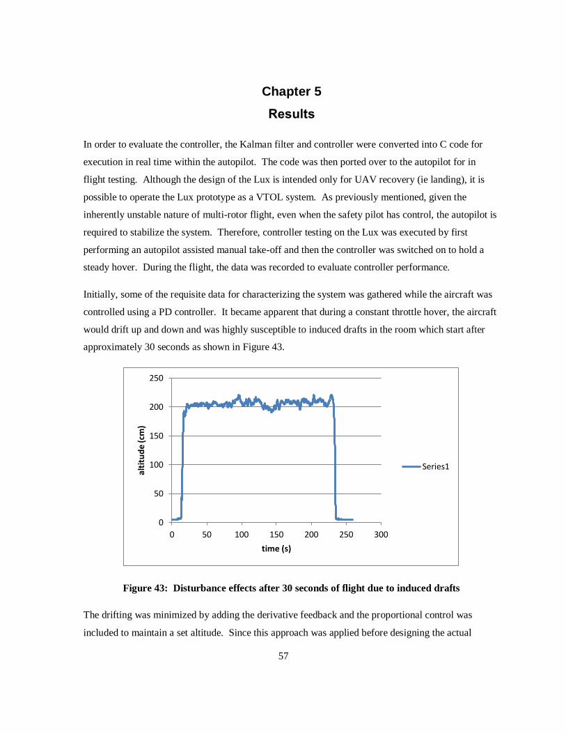
57

Chapter 5

Results

In order to evaluate the controller, the Kalman filter and controller were converted into C code for

execution in real time within the autopilot. The code was then ported over to the autopilot for in

flight testing. Although the design of the Lux is intended only for UAV recovery (ie landing), it is

possible to operate the Lux prototype as a VTOL system. As previously mentioned, given the

inherently unstable nature of multi-rotor flight, even when the safety pilot has control, the autopilot is

required to stabilize the system. Therefore, controller testing on the Lux was executed by first

performing an autopilot assisted manual take-off and then the controller was switched on to hold a

steady hover. During the flight, the data was recorded to evaluate controller performance.

Initially, some of the requisite data for characterizing the system was gathered while the aircraft was

controlled using a PD controller. It became apparent that during a constant throttle hover, the aircraft

would drift up and down and was highly susceptible to induced drafts in the room which start after

approximately 30 seconds as shown in Figure 43.

Figure 43: Disturbance effects after 30 seconds of flight due to induced drafts

The drifting was minimized by adding the derivative feedback and the proportional control was

included to maintain a set altitude. Since this approach was applied before designing the actual

0

50

100

150

200

250

0 50 100 150 200 250 300

alti

tud

e (c

m)

time (s)

Series1

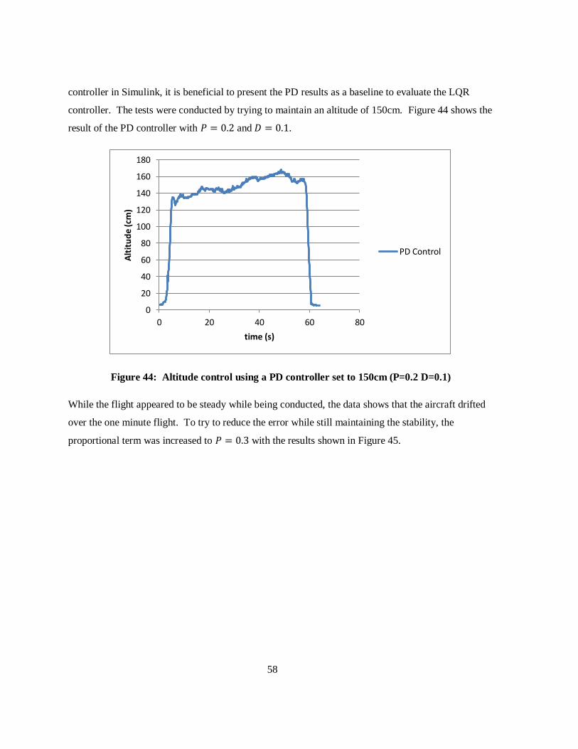
58

controller in Simulink, it is beneficial to present the PD results as a baseline to evaluate the LQR

controller. The tests were conducted by trying to maintain an altitude of 150cm. Figure 44 shows the

result of the PD controller with and .

Figure 44: Altitude control using a PD controller set to 150cm (P=0.2 D=0.1)

While the flight appeared to be steady while being conducted, the data shows that the aircraft drifted

over the one minute flight. To try to reduce the error while still maintaining the stability, the

proportional term was increased to with the results shown in Figure 45.

0

20

40

60

80

100

120

140

160

180

0 20 40 60 80

Alt

itu

de

(cm

)

time (s)

PD Control

59

Figure 45: Altitude control using a PD controller set to 150cm (P=0.3 D=0.1)

Once again, the flight appeared steady and the results are indeed better however the data

demonstrated a pronounced drift over time. The designed LQR control technique was then tested on

the system. Due to uncertainty about how the system would react with the new controller turned on,

the gains were recalculated using to penalize the control input and make the system a little

slower than the simulation response. Figure 46 shows the first LQR controller test set to an altitude

of 150cm.

0

20

40

60

80

100

120

140

160

180

0 20 40 60 80

alti

tud

e (c

m)

time (s)

PD Control

60

Figure 46: Altitude control using an LQR controller set to 150cm (R = 20)

The controller was stable and functioned as expected with the lower control input. To increase the

performance the LQR gains were recalculated with and the results are shown in Figure 47.

Figure 47: Altitude control using an LQR controller set to 150cm (R = 10)

The LQR controller test is by far the best performance achieved in any of the previous controllers.

The test was a minute long flight maintaining an error of less than 10cm which demonstrates the

0

20

40

60

80

100

120

140

160

180

0 20 40 60 80 100

alti

tud

e (c

m)

time (s)

LQR Control

0

20

40

60

80

100

120

140

160

180

0 20 40 60 80

alti

tud

e (c

m)

time (s)

LQR Controller

61

success of the approach. The PD controllers required much more tuning and still could not achieve

this tight control.

Next was to implement the LQR controller that was simulated using . The same step response

was applied to the system to compare implemented controller and system to the simulated model

shown in Figure 48.

Figure 48: Altitude step control using an LQR controller comparing actual to simulated (R = 5)

The experimental data and simulated response are in close agreement which indicates the identified

model is a close fit.

With the altitude control system working, the next step was to evaluate the results by implementing

the landing sequence. The key to the autonomous recovery is to use the developed control systems to

execute the required manoeuvres to transition from flight altitude to touchdown in a controlled

0 5 10 15 20 25 30 35140

160

180

200

220

240

260

altitude (

cm

)

Altitude

actual altitude

simulated altitude

0 5 10 15 20 25 30 35-100

-50

0

50

100

vert

ical velo

city (

cm

/s)

Vertical Velocity

time(s)

actual vertical velocity

simulated vertical velocity

62

manner that respects the limitations of the sensors used for altitude control. The main issues that

shaped the recovery sequence were:

The barometric altimeter is the only suitable sensor for altitude control above 3m AGL and

it is ideal for relative altitude measurement

The sonar sensor provides accurate and stable altitude measurements below 3m AGL and is

ideal for absolute altitude measurement giving the proper height AGL.

Altitude control within ground effect is highly non-linear so an alternative control approach

would be required

Considering these issues, the recovery sequence was divided into four distinct stages executed

sequentially to complete the automated recovery task.

Stage 1 - During the first stage, altitude control is conducted using the barometric altimeter. As was

mentioned earlier, this sensor provides high resolution readings that drift over time due to

atmospheric conditions. However, its relative accuracy is very good which makes it suitable for the

stage 1 constant descent manoeuver. The beginning of this stage is indicated by a command to the

autopilot to initiate autonomous descent. The prerequisite for this command is autonomous, non-

powered, forward flight with a sustained altitude glide used to bleed-off forward airspeed. The

autopilot initiates stage 1 flight when the UAV reaches an airspeed just above that which is associated

with a stall. When the stage is initiated, the current pressure altitude is sampled and supplied to the

descent controller and used as the current altitude set point. Then, using the pressure altitude

measurements a constant decent rate is maintained by linearly decreasing the pressure altitude set

point to maintain a constant descent rate.

Stage 2 – The objective of this stage is to decelerate the UAV at a constant rate to prepare for

touchdown. As the ultrasonic rangefinder gets near to the ground it starts to receive valid pings

indicating the absolute altitude AGL. During this time, the UAV is still in the constant descent of

stage 1. However the stage 2 Kalman filter, which uses different measurement noise covariance

associated with the sonar, is quickly converging as the sonar data becomes more reliable. At a

predefined altitude near the ground, stage 2 is initiated and the altitude control is switched to the

sonar measurements while the vertical descent rate is parabolically reduced until the aircraft enters

ground effect.

63

Stage 3 – Once the UAV is within ground effect, there is a sudden and drastic increase in lift. This

effect makes the current controllers unable to achieve touchdown. To ensure a graceful touchdown

stage 2 ensures the UAVs vertical velocity is nearly zero when it reaches the top of the ground effect.

Without this manoeuver, the UAV will bounce of the ground effect leading to difficult control prior to

touchdown. Stage 3 begins when the UAV is just in ground effect. Since ground effect is a function

of the UAVs distance from the ground, it is simple to control the UAV to touchdown by linearly

decreasing the throttle until the craft settles on the ground.

Stage 4 – Finally, immediately at touchdown the throttle is quickly ramped to zero to ensure the lift is

dramatically reduced thereby preventing the UAVs tendency to bobble on the ground during motor

wind-down. Figure 49 below shows the four stages of the autonomous fixed wing UAV recovery.

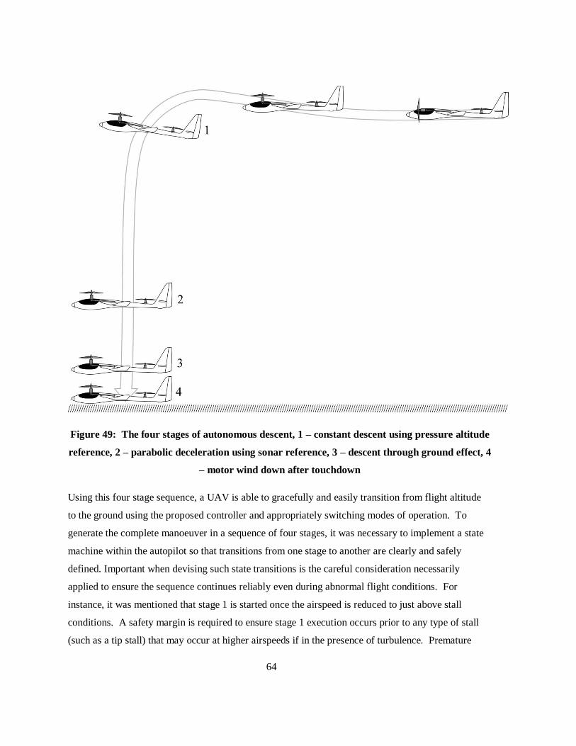
64

Figure 49: The four stages of autonomous descent, 1 – constant descent using pressure altitude

reference, 2 – parabolic deceleration using sonar reference, 3 – descent through ground effect, 4

– motor wind down after touchdown

Using this four stage sequence, a UAV is able to gracefully and easily transition from flight altitude

to the ground using the proposed controller and appropriately switching modes of operation. To

generate the complete manoeuver in a sequence of four stages, it was necessary to implement a state

machine within the autopilot so that transitions from one stage to another are clearly and safely

defined. Important when devising such state transitions is the careful consideration necessarily

applied to ensure the sequence continues reliably even during abnormal flight conditions. For

instance, it was mentioned that stage 1 is started once the airspeed is reduced to just above stall

conditions. A safety margin is required to ensure stage 1 execution occurs prior to any type of stall

(such as a tip stall) that may occur at higher airspeeds if in the presence of turbulence. Premature

65

stalling could lead to a condition of uncontrolled flight where the airspeed measuring device

(typically a pitot tube) maintains a higher airspeed then that which is required to initiate the descent

mode. While this example is somewhat contrived, it illustrates the careful consideration that must be

employed when considering autonomous state transitions. In any case, UAV control is designed and

required by governing agencies to ensure it is possible for the safety pilot to takeover should

autonomous flight run into such issues.

Prior to stage 1 execution presumably the autopilot is controlling the aircraft in forward flight mode

and is directing the aircraft on a path into the wind towards the landing site. At the appropriate time

the autopilot cuts the throttle and puts the motors into the vertical descent orientation. At this point,

the vertical descent mode is armed and triggered once the airspeed requirement is met. A level glide

is maintained by the autopilot, increasing angle of attack which necessarily causes the aircraft to slow

down. At the appropriate airspeed the vertical descent is triggered. This forward flight control is

simply mentioned so the reader understands the process leading up to the autonomous recovery.

However, this is not further discussed within this thesis. Through experimentation, it has been

determined that the actual airspeed when beginning the descent manoeuver is not critical however at

slower speeds the routine is clearly more graceful.

The state transition from stage 1 to stage 2 is largely dependent on the performance of the sonar

sensor employed. Given stage 2 requires the use of the ultrasonic rangefinder for the Kalman filter

measurement, it is a necessity that the UAV be close enough to the ground to be within the specified

range of the sonar. Also, the closer the UAV is to the ground the more reliable the measurements are.

Experiments using the Lux which has a 6m range sonar indicated that its sonar measurements were

consistent below 3m without erroneous pings received. Above 3m, there were erroneous

measurements that ranged from infrequent at 3m to often at 6m. The sonar reading accuracy is highly

dependent on numerous factors such as ground surface quality, pitch or roll angle of the aircraft,

ambient noise and possibility of nuisance echoes. By maintaining the stage 1 to stage 2 state

transition below 3m, it is likely the controller will have the benefit of pristine altitude measurements

to ensure reliable control.

The state transition from stage 2 to stage 3 required that it be determined experimentally given that

the ground effect in this case is largely due to the shape of the aircraft as well as the position of the

propulsion system. Slowing the aircraft prior to reaching ground effect is desirable in order to prevent

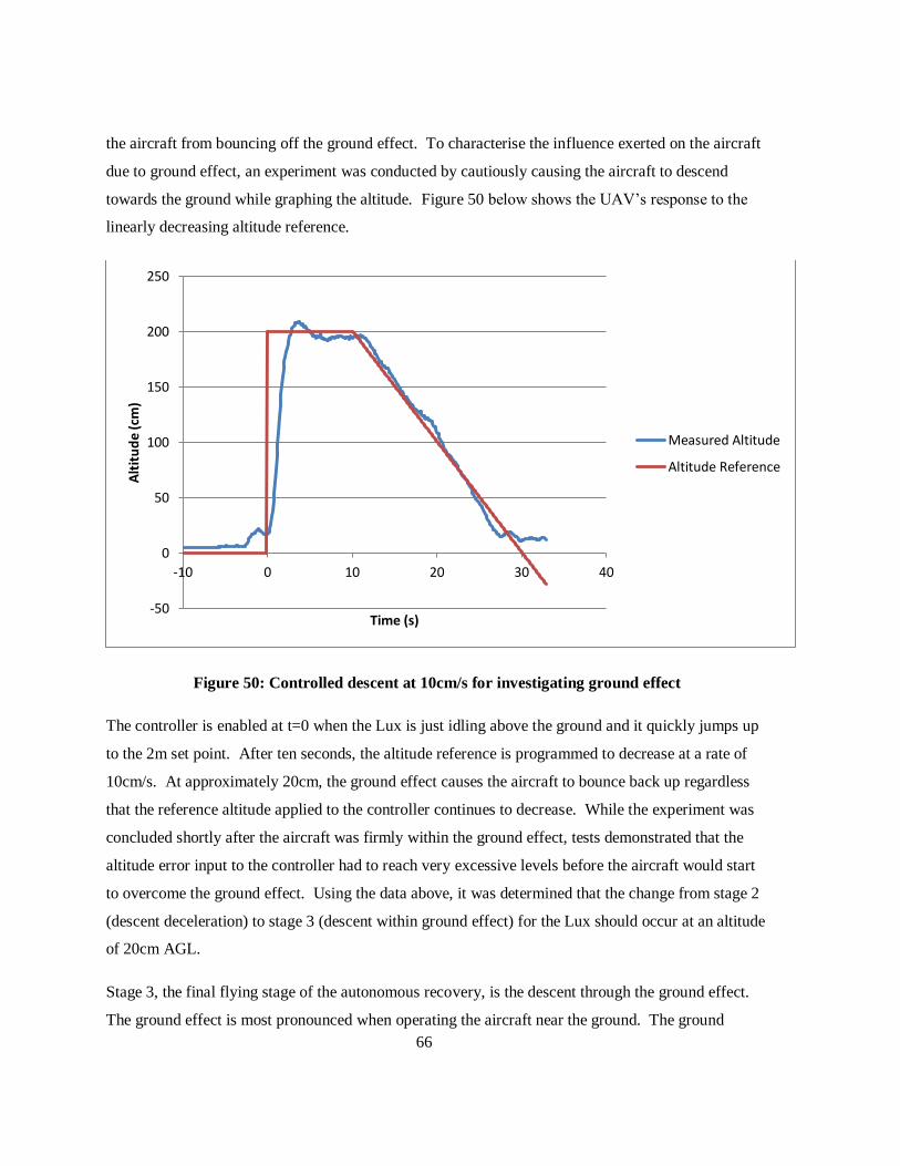
66

the aircraft from bouncing off the ground effect. To characterise the influence exerted on the aircraft

due to ground effect, an experiment was conducted by cautiously causing the aircraft to descend

towards the ground while graphing the altitude. Figure 50 below shows the UAV’s response to the

linearly decreasing altitude reference.

Figure 50: Controlled descent at 10cm/s for investigating ground effect

The controller is enabled at t=0 when the Lux is just idling above the ground and it quickly jumps up

to the 2m set point. After ten seconds, the altitude reference is programmed to decrease at a rate of

10cm/s. At approximately 20cm, the ground effect causes the aircraft to bounce back up regardless

that the reference altitude applied to the controller continues to decrease. While the experiment was

concluded shortly after the aircraft was firmly within the ground effect, tests demonstrated that the

altitude error input to the controller had to reach very excessive levels before the aircraft would start

to overcome the ground effect. Using the data above, it was determined that the change from stage 2

(descent deceleration) to stage 3 (descent within ground effect) for the Lux should occur at an altitude

of 20cm AGL.

Stage 3, the final flying stage of the autonomous recovery, is the descent through the ground effect.

The ground effect is most pronounced when operating the aircraft near the ground. The ground

-50

0

50

100

150

200

250

-10 0 10 20 30 40

Alt

itu

de

(cm

)

Time (s)

Measured Altitude

Altitude Reference

67

imposes a boundary layer which restricts the downwash shed from the motors thereby increasing the

effective lift without changing the RPM of the motors [27]. To descend through this area of increased

lift, the throttle is linearly ramped down and the aircraft slowly settles onto the ground. Figure 51

shows the autonomous descent and landing.

Figure 51: Descent manoeuvre and landing

The Lux was controlled manually to an altitude of about 260cm and then the controller was enabled.

After ten seconds, the navigation processor sends the Lux down at 40cm/s and initiates a constant

deceleration until the commanded altitude reaches 20cm. Immediately the throttle is ramped down

reducing the lift due to the ground effect which allows the Lux to settle onto the ground. This stage is

open loop control and the ramp rate determines how quickly the aircraft settles. Due to the nature of

open loop control, changes to the aircraft configuration or weight will have an effect on the resulting

performance.

Stage 4 occurs once the aircraft is on the ground and is simply a rapid throttle ramp down to turn the

motors off. This requirement ensures that a sudden gust of wind or another disturbance does not

cause the aircraft to hop back into the air.

The four stages presented here complete the autonomous recovery routine. Repeated indoor tests

have shown a gentle descent and touchdown when under autonomous control are able to be executed

with precision. The LQR controller, using a Kalman filter state feedback, has been proven to operate

reliably and on a consistent basis.

0

50

100

150

200

250

300

0 10 20 30 40

alti

tud

e (c

m)

time (s)

measured

reference

68

Chapter 6

Conclusions

This thesis explored the issue of autonomous fixed wing UAV recovery with the desire to provide a

safer means of concluding UAV missions. Current recovery techniques employed for UAV recovery

in developed areas was introduced with a brief discussion of their shortcomings. In order to

investigate alternatives, the experimental research airship called the Lux Aether, was introduced and

described as an alternative aircraft design employing vertical landing propulsion. A survey of

background and parallel research was provided. A short analysis on the experimental system

dynamics was undertaken and an approach to decoupled control was provided which allowed a more

focus treatment of the altitude associated plant and related control system. While not the focus of this

thesis, airframe stabilization was also presented indicating that developing a decoupled system

assumption with respect to the longitudinal and lateral dynamics, was reasonable. It was found that

PD control of the roll and pitch axis resulted in a stable system ideal for autonomous recovery

applications. A number of detail and solution approaches related to trimming the system were

introduced as a prerequisite to the system identification and controller design. Because the closed

loop control techniques depend greatly on the quality of the sensor readings, different sensor options

were explored. Based on both reliability and resolution, the barometric altimeter as well as the

ultrasonic rangefinder was recommended as feedback devices.

Various approaches to system identification were explored with varying success. It was identified

that using a least squares characterization did not provide accurate results in spite of the methodical

approach required to identify the unstable system. Running the system in open loop during the

identification process did generate a successful model. Using the system model and sensor variances,

a Kalman filter was designed which provided smooth and accurate data regarding system altitude and

vertical velocity states. Optimal state feedback control was first perfected in simulation and then

implemented within the Lux’s autopilot. Using LQR control techniques resulted in a very stable

system. The controller was compared with previous PD controller results and it was found that the

LQR was by far superior. The success of the LQR control approach validated the system modeling

techniques. It was demonstrated that by applying the approach to system identification and using the

LQR state feedback controller, the altitude mode could be successfully controlled enabling vertical

landing recovery of fixed wing UAV’s.

69

This thesis presents a novel vehicle that can be applied in current commercial UAV applications

which provides a built in recovery approach that is safer and more efficient then current fixed wing

UAV recovery techniques. This thesis also introduced a successful approach to VTOL modeling

techniques that could be generalized to other types of aircraft. Using this developed model, an

autonomous landing procedure was introduced that efficiently applies available sensor data to

generate a smooth and contiguous landing maneuver. All of the above techniques were validated by

testing on an actual aircraft system.

70

6.1 Future Research

For the specific stages of UAV recovery, the topic of this thesis, further investigation into optimizing

the recovery process for efficiency is an area where more investigation is required. Namely,

problematic was that when a mission was completed, the amount power left in the battery was

minimal due to current autonomous descent which demands a lot of power. While the focus of this

thesis was placed squarely on the control aspect of the recovery, the aircraft used was designed to

sustain lift for data gathering experiments and was generally overbuilt. Future revisions would look

at decreasing the size of the motors to better match the minimum requirements while optimizing the

propeller for both forward flight and vertical descent phases. Using this more optimized platform and

leveraging the control system explored in this thesis, more advanced descent manoeuvres could

possibly be explored. Ideally, this vertical UAV recovery system could use smaller motors that

simply stabilize the aircraft in a gravity powered descent and decelerate the craft prior to touch down.

This type of experimentation requires a solid control foundation to build upon since the experiments

would require hand launched flight to achieve altitude before the descent tests could be evaluated.

Once the descent is initiated, the aircraft is committed to the manoeuvre so there is a smaller margin

of error to ensure the aircraft is not lost to a crash.

Other future research could include investigating the transition from forward flight to vertical descent

under autopilot control. The stability and control of fixed wing aircraft flight dynamics are well

understood. The equations are based on aerodynamic derivatives which influence the system

according to states of the system such as angle of attack and sideslip. These techniques are heavily

based on the velocity and orientation of the wind frame with respect to the body frame. At the very

low airspeeds encountered when transitioning to descent mode these equations start to break down

since the derivatives are generated by linearizing the system about an operating point. To robustly

operate a control scheme from forward flight to vertical descent, a unique topology would have to be

explored to handle the transition.

The research in this thesis has demonstrated a model structure with proven accurate control results.

Further research into the suitability of adaptive control would be beneficial. Using adaptive control

techniques, changes in the aircraft structure or payload would be accounted for without having to redo

the system identification. Leveraging the developed model, adaptive control techniques could be

applied for the model parameter identification. Future research would extend the capabilities of the

71

system. Further research could lead to online parameter identification or an offline method used for

autonomous tuning of the system.

The Lux Aether UAV has extended the possible applications of efficient fixed wing

UAVs. Anywhere a helicopter or multi-rotor UAV can operate is now an ideal location to conduct

fixed wing UAV missions. In northern areas, where the landscape is either forested or covered by

undulating rocks, missions can now be conducted out of a small clearing. Longer range fixed wing

operations such as dropping GPS transponders on icebergs can now be conducted on the oceans using

vessels that are not designed for fixed wing aircraft recovery. Finally, a major benefit of the system is

the autonomy. The most difficult part of flying conventional aircraft is the landing, by automating the

landing procedure, the UAV applications can extend to those which do not require qualified pilots.

72

References

[1] M. Degarmo and G. Nelson, "Prospective Unmanned Aerial Vehicle Operations in the Future

National Airspace System," in AIAA 4th Aviation Technology, Integration and Operations

(ATIO) Forum, Chicago, Illinois, Sep. 20-22, 2004.

[2] (March, 2013) Accuas. [Online]. http://www.accuas.com

[3] (2013, March) Unmanned Systems Canada - Student UAV Competition. [Online]. Internet:

http://www.unmannedsystems.ca/content.php?sec=8

[4] P. G. Fahlstrom and T. J. Gleason, Introduction to UAV Systems, 4th ed., John Wiley & Sons

Ltd, Ed. Chichester, UK: John Wiley & Sons Ltd, 2012.

[5] J. Rumerman. (2010, December) Early helicopter technology.

[6] J. G. Leishman. (2000) The history of helicopter flight. [Online].

http://terpconnect.umd.edu/~leishman/Aero/history.html

[7] J. G. Leishman, Principles of helicopter aerodynamics. New York, NY: Cambridge University

Press, 2000.

[8] O. Stewart, "New ways of flying: the Trueman Wood lecture," Journal of the Royal Society of

Arts, pp. 626-640, May 1955.

[9] D. L. Kohlman, Introduction to V/STOL airplanes. Ames, IA: Iowa State University Press, 1981.

[10] T. McLelland, Harrier. Birmingham, UK: Ian Allan Publishing, 2011.

[11] Julian. (2013, March) Harrier and F-35B. [Online].

http://juliantheaviator.wordpress.com/2008/01/15/harrier-and-f-35/

[12] V. Fuertes, A. Piquereau, R. Mampey, and F. Teichteil-Königsbuch P. Fabiani, "Autonomous

flight and navigation of VTOL UAVs: from autonomy demonstrations to out-of-sight flights,"

Aerospace Science and Technology, vol. 11, no. 2, pp. 183-193, 2007.

[13] J. H. Lee, B. J. Kim,H. J. Kwon,E. T. Kim, A. Iee-Ki P. S. Kim, "Automatic Landing Control

Law for Unmanned Helicopter using Lyapunov Approach," 25th Digital Avionics Systems

Conference, vol. 1, no. 8, pp. 15-19, October 2006.

[14] C. Ham, Z. Qu, J. Kaloust, "Nonlinear autopilot control design for a 2-DOF helicopter model,"

Control Theory and Applications, IEEE Proceedings, vol. 144, no. 6, pp. 612-616, November

1997.

73

[15] J. F. Montgomery, G. Sukhatme, S. Saripalli, "Vision-based autonomous landing of an

unmanned aerial vehicle," IEEE International Conference on Robotics and Automation,

Proceedings, vol. 3, pp. 2799 - 2804 , 2002.

[16] J. Stumpf, M. Achtelik, K. M. Doth, G. Hirzinger, D. Rus D. Gurdan, "Energy-efficient

Autonomous Four-rotor Flying Robot Controlled at 1 kHz," in 2007 IEEE International

Conference on Robotics and Automation, April 2007, pp. 361-366.

[17] R. Siegwart S. Bouabdallah, "Backstepping and Sliding-mode Techniques Applied to an Indoor

Micro Quadrotor,"" in Proceedings of the 2005 IEEE International Conference on Robotics and

Automation, 2005, pp. 2247-2252.

[18] E. Altug B. Erginer, "Modeling and PD Control of a Quadrotor VTOL Vehicle," in 2007 IEEE

Intelligent Vehicles Symposium, 2007, pp. 894-899.

[19] (2012, March) CropCam images on demand. [Online]. http://www.cropcam.com

[20] G. M. Y. Lai, "Modelling and control of small-scale helicopter on a test platform," Doctoral

Thesis - University of Waterloo, 2008.

[21] Q. G. Wang, Decoupling Control. Berlin, Germany: Springer, 2003.

[22] B. Etkin, Dynamics of Atmospheric Flight. New York: John Wiley & Sons, 1972.

[23] R. W. Beard and T. W. McLain, Small Unmanned Aircraft Theory and Practice. Princeton, NJ:

Princeton University Press, 2012.

[24] R. C. Nelson, Flight Stability and Automatic Control, 2nd ed. Boston, MA: McGraw-Hill, 1998.

[25] G. Welch and G. Bishop, "An Introduction to the Kalman Filter," In Practice, vol. 7, no. 1, pp.

1-16, July 2006.

[26] R. C. Dorf and R. H. Bishop, Modern Control Systems, 11th ed. Upper Saddle River, NJ:

Pearson Prentice Hall, 2008.

[27] B. Etkin and L. D. Reid, Dynamics of Flight stability and control. Danvers, MA: John Wiley and

Sons, 1996.