Embed Size (px)
Citation preview

Autumn 2002
microeconomics economic theory
& applications1

MSc Economics
Birkbeck College
Economic Theory and Applications I
Lecture NotesAutumn 2002
Preface
Aims
This first block of the Economic Theory course aims to familiarize students withbasic tools in microeconomic theory, and enable them to apply these tools tosolve problems in public policy. The lectures aim to promote the ability to thinkin a structured framework, and clarify the importance of formal arguments.An important aim of the course is to demonstrate the art of formal modelingwhich requires simplifying a problem by identifying the key elements withoutoversimplifying and trivializing the issue.
Objectives
The students should be able to demonstrate that they:
• can solve the optimization problems faced by consumers and producersunder certainty as well as uncertainty
• can derive the general equilibrium of specific economies
• can apply the basic solution concepts in game theory
• can solve for optimal contracts under adverse selection and moral hazard
• can solve for optimal bidding behaviour in standard auctions
• can explain the effect of externalities and missing markets
• can specify Groves mechanisms to solve public good provision problems
Teaching Arrangements
The course is taught over 10 weeks. There is a double lecture on Tuesdayevenings, from 6-9 pm, and a lecture on Wednesday, from 6 to 7.30 pm. Inaddition, there is a weekly class for discussing solutions to the problem sets.Answers to problem sets 1-4 (the first part of the ETA 1 course) will be madeavailable after they are discussed in class. Alternatively, as soon as discussed
i

Birkbeck Economics ii
in class, they can be downloaded from the course web-site athttp://www.bbk.ac.uk/ems/econ/courses/msceconomics/mscecon.htm. Theanswers to the remaining problem sets will be discussed in the classes, and writ-ten solutions will be made available before the review sessions in May 2002. Thisdelay is partly to encourage you to solve through the problems without the helpof written solutions - as the questions from the second half of the course aretechnically much less demanding compared to the first half - but conceptuallymore demanding, and also because the problems in the first half tend to repre-sent a broad class of problems, while those from the second half are much morespecific.
Course Assessment
80% of the final grade for this course is determined through a three-hour exam-ination in June, and the rest on assessment of course-work. The course workassessment is based on the following:
• A ‘take-home’ Christmas assignment contributes 10%.
• Two ‘in-class’ quizzes are held during term. The higher of the two markscontributes 10%.
Texts
The lectures draw on material from a variety of sources, including the followingtexts (available at Waterstones on Gower street). Some other readings arepointed out in the lecture schedule below. Additional handouts will be provided.
• Geoffrey Jehle and Philip Reny, Advanced Economic Theory, Addison-Wesley, 1998
• Hal Varian, Microeconomic Analysis, 3rd edition, Norton, 1992
• Bernard Salanie, The Economics of Contracts, MIT Press, 1997.
• Debraj Ray, Development Economics, Princeton University Press, 1998.
• Avinash Dixit and Susan Skeath, Games of Strategy, Norton, 1999.
• Watson, Joel, Strategy, Norton, 2002.
A Preliminary Schedule of Lectures
• Weeks 1-2 Basic consumer theory and producer theory, choice underuncertainty.

Birkbeck Economics iii
• Weeks 3-5 General equilibrium analysis.
• Week 5 Class test
• Week 6 Game theory.
• Week 7 Adverse selection and contracts. Applications to markets forcredit and insurance.
• Week 8 Moral hazard and contracts.
• Weeks 9-10 Auction theory. Externalities and public goods. Mechanismdesign - Groves mechanism. Class test.
If you have any queries about the course, you should contact us.
Hope you enjoy the course!
Arup Daripa ([email protected])Ji Hong Lee ([email protected])

Contents
Preface i
1 Theory of choice: an axiomatic approach 1
1.1 Preference Relations . . . . . . . . . . . . . . . . . . . . . . . . . 1
1.2 Two induced relations . . . . . . . . . . . . . . . . . . . . . . . . 2
1.3 Possible Properties of Preference Relations . . . . . . . . . . . . 2
1.4 Existence of a Utility Function . . . . . . . . . . . . . . . . . . . 2
1.5 A further property . . . . . . . . . . . . . . . . . . . . . . . . . . 3
2 Utility Maximisation 4
2.1 The consumer’s problem: utility maximisation . . . . . . . . . . 4
2.2 Expenditure Minimisation . . . . . . . . . . . . . . . . . . . . . . 5
2.3 Demand Functions . . . . . . . . . . . . . . . . . . . . . . . . . . 6
2.4 Some Identities and Relations . . . . . . . . . . . . . . . . . . . . 6
2.5 An application: the neoclassical model of labour supply . . . . . 9
3 Producer Theory: an Overview 10
3.1 Technology . . . . . . . . . . . . . . . . . . . . . . . . . . . . . . 10
3.2 (Possible) Restrictions on the Technology Set . . . . . . . . . . . 11
3.3 Returns to Scale . . . . . . . . . . . . . . . . . . . . . . . . . . . 11
3.4 Profit Maximisation . . . . . . . . . . . . . . . . . . . . . . . . . 11
3.5 Cost Minimisation . . . . . . . . . . . . . . . . . . . . . . . . . . 13
3.6 Duality . . . . . . . . . . . . . . . . . . . . . . . . . . . . . . . . 14
4 Choice under Uncertainty 15
4.1 Some notation . . . . . . . . . . . . . . . . . . . . . . . . . . . . 15
4.2 Preferences over lotteries: some axioms . . . . . . . . . . . . . . . 16
4.3 The Representation Theorem (informal) . . . . . . . . . . . . . . 16
4.4 Risk Aversion . . . . . . . . . . . . . . . . . . . . . . . . . . . . . 17
4.5 Measures of Risk Aversion . . . . . . . . . . . . . . . . . . . . . . 17
iv

Birkbeck Economics v
4.6 Measures of Risk . . . . . . . . . . . . . . . . . . . . . . . . . . . 18
4.7 An Example: The Demand for Insurance . . . . . . . . . . . . . . 18
4.8 The Allais Paradox . . . . . . . . . . . . . . . . . . . . . . . . . . 19
5 Exchange and General Equilibrium 20
5.1 Allocations and Exchange . . . . . . . . . . . . . . . . . . . . . . 20
5.2 Walrasian equilibrium . . . . . . . . . . . . . . . . . . . . . . . . 21
5.3 The Existence of Walrasian equilibrium . . . . . . . . . . . . . . 22
5.4 Existence of Walrasian equilibria . . . . . . . . . . . . . . . . . . 23
5.5 Pareto efficient allocations . . . . . . . . . . . . . . . . . . . . . . 23
5.6 The welfare theorems . . . . . . . . . . . . . . . . . . . . . . . . . 23
5.7 Incorporating Production . . . . . . . . . . . . . . . . . . . . . . 25
6 Game Theory 27
6.1 Games in Normal (or Strategic) Form . . . . . . . . . . . . . . . 28
6.2 Dominance and Iterated Dominance . . . . . . . . . . . . . . . . 28
6.3 Weak Dominance . . . . . . . . . . . . . . . . . . . . . . . . . . . 29
6.4 Nash Equilibrium . . . . . . . . . . . . . . . . . . . . . . . . . . . 30
6.5 Nash Equilibrium in Mixed strategies . . . . . . . . . . . . . . . 31
6.6 Games in Extensive Form . . . . . . . . . . . . . . . . . . . . . . 32
6.7 Actions and Strategies . . . . . . . . . . . . . . . . . . . . . . . . 34
6.7.1 Game1 . . . . . . . . . . . . . . . . . . . . . . . . . . . . . 34
6.7.2 Game2 . . . . . . . . . . . . . . . . . . . . . . . . . . . . . 35
6.8 Analyzing Extensive Form Games . . . . . . . . . . . . . . . . . . 35
6.9 Equilibrium Refinement . . . . . . . . . . . . . . . . . . . . . . . 36
6.10 Games of Incomplete Information . . . . . . . . . . . . . . . . . . 38
6.11 Repeated Games and the Folk Theorem . . . . . . . . . . . . . . 38
6.12 Some game-theoretic models of oligopoly . . . . . . . . . . . . . . 39
6.13 Bertrand Equilibrium: Nash equilibrium in prices . . . . . . . . . 39
6.14 Cournot equilibrium: Nash equilibrium in quantities . . . . . . . 41
6.15 Duopoly with sequential moves: the Stackelberg equilibrium . . . 41
7 Topics in Information Economics: Adverse Selection 43
7.1 Introduction . . . . . . . . . . . . . . . . . . . . . . . . . . . . . . 44
7.2 Akerlof’s Model of the Automobile Market . . . . . . . . . . . . . 45
7.3 Adverse Selection and Contracts . . . . . . . . . . . . . . . . . . 46
7.3.1 Adverse Selection: Description of the Problem . . . . . . 46

Birkbeck Economics vi
7.3.2 First Best: No Information Problem . . . . . . . . . . . . 47
7.3.3 Saying It with a Picture . . . . . . . . . . . . . . . . . . . 48
7.3.4 A Separating Solution . . . . . . . . . . . . . . . . . . . . 50
7.3.5 A Pooling Solution . . . . . . . . . . . . . . . . . . . . . . 52
7.3.6 Existence of Separating and Pooling Solutions With Mul-tiple Insurers . . . . . . . . . . . . . . . . . . . . . . . . . 55
7.4 Signaling . . . . . . . . . . . . . . . . . . . . . . . . . . . . . . . 58
8 Topics in Information Economics: Moral Hazard 59
8.1 Introduction . . . . . . . . . . . . . . . . . . . . . . . . . . . . . . 59
8.2 A formalization . . . . . . . . . . . . . . . . . . . . . . . . . . . . 60
8.3 The principal’s problem . . . . . . . . . . . . . . . . . . . . . . . 62
8.4 Observable effort . . . . . . . . . . . . . . . . . . . . . . . . . . . 62
8.5 Unobservable effort . . . . . . . . . . . . . . . . . . . . . . . . . . 63
9 Topics in Information Economics: Application to Micro-CreditDesign 65
10 Auction Theory 67
10.1 Auctions Under Independent Private Values . . . . . . . . . . . . 68
10.1.1 Revenue Equivalence . . . . . . . . . . . . . . . . . . . . . 68
10.1.2 Vickrey Auction . . . . . . . . . . . . . . . . . . . . . . . 68
10.1.3 First Price Sealed Bid Auction . . . . . . . . . . . . . . . 69
11 Externalities and Market Failure 71
12 Provision of Public goods 72
13 Mathematical Appendix 74
M.4 Open and Closed sets . . . . . . . . . . . . . . . . . . . . 74
M.5 Compactness . . . . . . . . . . . . . . . . . . . . . . . . . 75
M.6 Continuous Functions . . . . . . . . . . . . . . . . . . . . 75
M.7 Weierstrass’ Maximum Theorem . . . . . . . . . . . . . . 75
M.8 Berge’s Maximum Theorem . . . . . . . . . . . . . . . . . 75
M.9 The Envelope Theorem . . . . . . . . . . . . . . . . . . . 76

Chapter 1
Theory of choice: an axiomatic approach
1. On modelling choice. The objects of choice. Consumer choice.
2. Preference relations: binary relations as building-blocks.
3. The basic axioms: reflexivity, completeness and transitivity.
4. Numerical representations of preference: utility functions.
5. Monotonicity, continuity and the existence of utility functions.
6. The ordinal nature of utility functions.
7. One further axiom: the convexity of preferences.
8. Graphical representation of preferences: indifference curves.
Readings
1. Varian, 7.1.
2. Jehle & Reny, 3
3. Deaton & Muellbauer: Economics and Consumer Behaviour, Ch 2.1
1.1 Preference Relations
A binary relation defined on a set X is a set of ordered pairs in X. For example,the following are binary relations: x is taller than y; x is as tall as y.
Consider an individual who must choose one alternative from a set X. Considerany two arbitrary x, y ∈ X. Suppose the individual considers outcome x to beat least as good as outcome y. This is written as x R y, or sometimes as x R y.Then R is a binary relation on the set X, and is called a weak preference relation.
1

Birkbeck Economics 2
1.2 Two induced relations
1. Strong Preference Relation: We say that x is strictly preferred to y,written as x P y, if and only if
x R y and not y R x.
2. Indifference Relation: We say that x is considered indifferent to y,written as x ∼ y if and only if
x R y and y R x.
1.3 Possible Properties of Preference Relations
Consider a preference relation R defined on a set X
1. It is said to be reflexive on X if x R x for all x ∈ X.
2. It is said to be complete on X if for all x, y ∈ X,
either x R y or y R x or both.
3. It is said to be transitive on X if for all x, y, z ∈ X
x R y and y R z implies x R z.
Properties 1 to 3 are called the rationality axioms.
4. Continuity of preferences. For all y ∈ X, the sets {x : x R y} and{x : y R x} are closed1.
5. Strong monotonicity. If x ≥ y, and x �= y, then x P y.
1.4 Existence of a Utility Function
Suppose preferences are complete, reflexive, transitive, strongly monotonic andcontinuous. Then, there exists a continuous utility function which represents(or describes) those preferences. That is, there exists a function u : X → Rsuch that
u(x) ≥ u(y) if and only if x R y.
The function u(·) is ordinal.1A set X is said to be closed if every convergent sequence in X converges to a point in X.
Less formally, a closed set contains its boundary points. A set that is not closed is open. See
the mathematical appendix for a formal definition.

Birkbeck Economics 3
1.5 A further property
6. Convexity of preferences. Preferences are said to be convex if for allx, y, z ∈ X such that x R z and y Rz, we have
(tx + (1 − t)y) R z for all 0 ≤ t ≤ 1

Chapter 2
Utility Maximization
1. The consumer’s problem: utility maximization. The indirect utility func-tion, and its properties.
2. Expenditure minimization. The expenditure function, and its properties.
3. Hicksian vs Marshallian demand functions.
4. The envelope theorem.Roy’s Identity and the Slutsky equation.
5. Applications: taxation and savings.
Readings
We rely heavily on the optimization techniques covered in the QuantitativeTechniques course. For the specifics, see
1. Varian 7, 8, and 9.
2. JR 3.
3. Deaton, A., and J. Muellbauer, Economics and Consumer Behaviour, 2(‘Preferences and Demand’), and 4 (‘Extensions to the basic model’)
2.1 The consumer’s problem: utility maximization
Let x ∈ Rn be a ‘bundle’ of commodities, and let X denote the set of all suchbundles. Consider a consumer who has a preference pre-ordering over this setX; The consumer’s problem is to choose the best consumption bundle x (interms of her preferences) subject to a budget constraint. Let pj denote theprice of the j − th good, and p = (p1, p2, . . . , pn) denote the vector of prices.We assume the consumer is ‘too small’ to influence the price vector throughher choices so that it can be taken as parametric relative to those choices. Forany consumption choice x, the total expenditure is given as the inner productp ·x. The budget constraint specifies an upper limit on the expenditure, so thatp · x ≤ m, where m is income or wealth.
4

Birkbeck Economics 5
Recall that if the consumer’s preferences satisfy completeness, reflexivity, tran-sitivity and continuity, they can be represented numerically by a continuousutility function U(x); recall our discussion on the representation theorem, thefirst one. If so, the consumer’s problem is reduced to the following:
maxx U(x) such that p · x ≤ m. (UMax)
In general a solution exists if all prices are strictly positive and income is notunbounded above. If, additionally, we assume the preferences to be strictlyconvex, the solution is unique. If they are locally non-satiated, we can showthat the budget constraint will bind, i.e., at the optimal choice x∗, we musthave p · x∗ = m.
Given that a solution exists, we can define an optimal value function as fol-lows. If x∗(p, m) solves (UMax) at prices p and income m, we can defineU(x∗(p, m)) ≡ v(p, m). The function v(p, m), which measures the maximizedvalue of utility at (p, m), is called the indirect utility function. Notice that,since a utility function is arbitrary, any monotonic transformation of a util-ity function is itself a legitimate utility function. The indirect utility functioninherits this property.
Given the manner in which the indirect utility function is constructed – it is theoutcome of a maximization exercise – certain properties follow. The indirectutility function is
1. homogeneous of degree 0 in p and m,
2. weakly decreasing in p and weakly increasing in m,
3. quasi-convex in p,
4. continuous at all p > 0, m > 0.
2.2 Expenditure Minimization
We now consider a related problem. Suppose we ask the following question.Given prices p, and a utility function U(·), what is the minimum amount ofmoney needed to attain, say, the level of utility u. Formally, the problem is asfollows
minx p · x subject to U(x) ≥ u, x ≥ 0. (EMin)
Provided the level of utility u is achievable, this problem too has a solution.And once again, if U represents preferences that are strictly convex, the solutionis unique. Of course, regardless of whether the solution is unique, we can obtainan optimal value function. Since the (EMin) problem is parameterized by pricesp and a target level of utility u, we define the expenditure function e(p, u) tomeasure the minimum amount of expenditure needed to obtain a utility levelu at prices p. As an exercise, try and establish the following properties for anexpenditure function.

Birkbeck Economics 6
1. e(p, u) in homogeneous of degree one in p,
2. e(p, u) is weakly increasing in p and strictly increasing in u,
3. e(p, u) is concave in p.
2.3 Demand Functions
Suppose the solution to the utility maximization problem is unique. (Can youthink of a simple case where uniqueness cannot be guaranteed?) The solutionx∗(p, m) of the utility maximization problem is, in effect, the demand function.The i− th component of this vector is the demand for the i− th commodity asa function of all prices and the income level m. The vector of demands x∗(p, m)is known as the Marshallian (or market) demand function.
Now consider the expenditure minimization problem. Once again, assume thesolution to be unique, and let it be given by the vector h(p, u); notice that theproblem is now parametrized by p and u, so that the solution is a function ofthese variables. The vector h(·), too, can be interpreted as a vector of demands,though it is an unusual one. The i−th component of this measure the amount ofcommodity i demanded at prices p if a target level of utility u is to be attained.It is akin to the conditional factor demand functions in producer theory. Inorder to distinguish it from the standard demand function, this is called theHicksian (or sometimes, the compensated) demand function.
If the expenditure function is differentiable in prices, Proposition 1 follows fromstandard envelope theory arguments. You should try to construct a proof.
Proposition 1 For p > 0, we have∂e(p, u)
∂pi= hi(p, u)
2.4 Some Identities and Relations
In what follows, we assume the utility maximization problem and the expen-diture minimization problems have unique solutions at all (p, m) and (p, u),respectively. We also assume that the expenditure function and indirect util-ity function are twice differentiable, and the Hicksian and Marshallian demandfunctions are continuously differentiable.
Consider the utility maximization problem, and let x∗(p, m) solve the problemat prices p and income m. Set U(x∗) = u∗. Suppose we now consider theproblem of trying to minimize the expenditure in order to attain the level ofutility u∗. It is clear that if u∗ is the maximum level of utility attainable withincome m (at prices p), then the minimum level of expenditure to attain u (atthe same prices p) must equal m. In other words, e(p, u∗) ≡ m. Notice thatthe result holds as an identity. We have other such identities, which we statebelow. We begin with a restatement of the identity just discussed.

Birkbeck Economics 7
1. e(p, v(p, m)) ≡ m.
2. v(p, e(p, u)) ≡ u.
3. x(p, m) ≡ h(p, v(p, m)).
4. h(p, u) ≡ x(p, e(p, u)).
These identities allow us to discover further relations, say, between the indirectutility function and Marshallian demand, and between the price derivatives ofHicksian and Marshallian demand. We consider these in turn. First, we haveRoy’s Identity, another result based on the envelope theorem, which relates theindirect utility function to Marshallian demand. Assuming differentiability, wehave
Proposition 2 (Roy’s identity) For p > 0, m > 0, we have
xi(p, m) = − (∂v/∂pi)(∂v/∂m)
Since this result seems a little different from the envelope theorem argumentsthat you have seen so far (and justifiably so), we will outline a proof. Supposex∗(p, m) solves (UMax) at (p, m). Set U(x∗(p, m)) = u∗. Then, by identity (2)above we have,
v(p, e(p, u∗)) = u∗ for a fixed u∗ and all p.
Differentiating this identity with respect to pi, we get
∂v
∂pi+
∂v
∂m
∂e
∂pi= 0.
But∂e
∂pi
∣∣∣∣p,u∗
= hi(p, u∗) = xi(p, m)
where the first equality follows from Proposition 1, and the second from theidentity (3) (or (4)) listed above. Substituting in the above relation and rear-ranging, the result follows. //
The second relationship that we consider concerns the price derivatives of Hick-sian and Marshallian demand, a relationship that is usually referred to as theSlutsky equation. Consider any (p, m). Let xj(p, m) denote the Marshalliandemand, and let hj(p, v(p, m)) denote the Hicksian demand at prices p and thelevel of utility attained at that Marshallian demand. Then,
Proposition 3 (Slutsky Decomposition)
∂xj
∂pi=
∂hj
∂pi− xi
∂xj
∂m.

Birkbeck Economics 8
The proof is straightforward; suppose, as before, x∗(p, m) solves (UMax) at(p, m) and set U(x∗(p, m)) = u∗. This time we start with identity (4) hj(p, u) ≡xj(p, e(p, u)).
Differentiate with respect to pi to get
∂hj
∂pi=
∂xj
∂pi+
∂xj
∂m
∂e
∂pi
Once again, (∂e/∂pi) = hi(·), which, evaluated at u∗, equals xi(p, m). Substi-tuting, and rearranging we get the required expression. //
The Slutsky equation permits an intuitive interpretation. Effectively, it allows anotional decomposition of the effect of a change in price on Marshallian (market)demand. An increase in the price of any commodity, say, in pi, has two effects.One, it changes the relative price between the various commodities, and two,it decreases the overall level of real income for any consumer who purchases apositive quantity of the i−th commodity. The effect on demand can thereby bebroken into two components. The first component, captured by ∂hj/∂pi in theSlutsky relation, measures the substitution effect on the demand for the j − thcommodity when the i− th price changes, if we were to keep the level of utilityunchanged. The second component, −xi(∂xj/∂m), captures the income effectof the price change.
The Slutsky equation allows us to characterize certain properties that demandfunctions must, in theory, possess. Recall that, by proposition 1, the Hicksiandemand for the j− th commodity can be obtained by differentiating the expen-diture function with respect to the pj . Assuming the expenditure function istwice differentiable, we can evaluate ∂hj/∂pi as ∂2e/(∂pi∂pj). Since we knowthat the expenditure function is concave in prices, we know that the matrix of itssecond-order partial derivatives is negative semi-definite; and as a corollary ofnegative semi-definiteness, the own-price cross-partial ∂2e/(∂pi∂pi) = ∂hi/∂pi
is non-positive. Further, the matrix of second-order partial derivatives is alwayssymmetric.
We have thus obtained theoretical restrictions on the substitution terms, ∂hj/∂pi.Given the Slutsky equation, these terms are nothing but the sum (∂xj/∂pi +xi∂xj/∂m), so that we now have the same restrictions on this term composedof Marshallian demand functions.
Some further terminology allows us to classify goods in terms of demand re-sponses to parametric changes. A good j is said to be
1. an inferior good if ∂xj/∂m < 0,
2. a normal good if ∂xj/∂m > 0,
3. a Giffen good if ∂xj/∂pj > 0,
4. a necessary good if 0 ≤ ∂xj/∂m < xj/m,
5. a luxury good if xj/m ≤ ∂xj/∂m.

Birkbeck Economics 9
2.5 An application: the neoclassical model of labour
supply
We now consider an application of our theory of choice. Suppose consumptionis financed out of two ‘sorts’ of income: the first source is labour income, whichdepends on the work effort � of the individual, and the wage rate w at whicheffort is rewarded; the second source of income is independent of the effort level,which we call non-labour income, y. Total income equals y + w�, so that thebudget constraint is now written as px = y + w�. (Assume local-non-satiation,so that we can write the budget constraint as an equality). Of course, given thespecification, it is reasonable to impose an additional constraint in the utilitymaximization problem, namely that 0 ≤ � ≤ �0, where �0 represents maximumlabour time available.
It is convenient to think of (�0 − �) as the total leisure time. In fact, one caneven go further and think of leisure as a consumption good in itself. Define(�0 − �) ≡ x0; the vector x = (x1, x2, . . . xn) now refers to consumption goodsother than leisure. We then write the utility function as U(x0, x), which issimilar in structure to the utility functions we have seen so far. Notice, also,that the wage rate w can then be viewed as the price of leisure. So the utilitymaximization problem is to maximize U(�0 − �, x) subject to px = y + w� and0 ≤ � ≤ �0. This is the same as
Maximize U(x0, x) subject to px + wx0 = y + w�0 and 0 ≤ x0 ≤ �0.
The problem admits a standard solution and we can obtain Marshallian de-mand functions, x∗
0(p, w, y + w�0) and x∗(p, w, y + w�0). We can also define theassociated expenditure minimization problem and obtain the Hicksian demandfunctions, h0(p, w, u) and h∗(p, w, u).
The aim is to develop the Slutsky equation for leisure which differs slightlyfrom the Slutsky equations we met earlier. This is because the problem itselfis a little different: here, the effect of changing the price of leisure is morecomplicated, since the change affects both sides of the budget equation.
The Slutsky equations for leisure:
∂x∗0
∂w=
∂h0
∂w+ �
∂x∗0
∂m∂x∗
0
∂pi=
∂h0
∂pi− xi
∂x∗0
∂m

Chapter 3
Producer Theory: an Overview
1. Technology. Restrictions on technology sets. Returns to scale.
2. Profit maximisation. Properties of profit functions. Hotelling’s Lemma.
3. Cost minimisation. Properties of cost functions. Shephard’s lemma.
4. An introduction to duality.
Readings
1. Varian 1-6. A good book for this material. Six chapters of a text-bookmay seem a bit much for one topic. but much of it will be familiar.
2. JR 5
3.1 Technology
A production plan is an n-dimensional vector, that is, y ∈ Rn. The j − thcomponent yj of this vector indicates the net output of the j − th good in thegiven production plan: if yj > 0, the j− th good is an output of the productionplan; if yj < 0, the j − th good is an input. Naturally, many of the componentsin any production plan may be zero.
Notice that a production plan is just any vector y. Some plans are clearlyunrealistic; for instance, if the plan contains inputs in too small a quantity toproduce the planned level of output(s), it is not feasible. Of course, what isfeasible and what is not depends on the technological state of the economy. Aproduction possibility set Y is the set of all feasible production plans. Typically,it is a very large set of vectors.
Sometimes production possibilities are written in a manner which seems moreintuitive, at least for plans which involve only one output and one or moreinputs. In that case, the output can be written as the scalar y, and the inputvector as x, so that a production plan then writes as (y,−x). This also allowsus to define the input requirement set V (y) as the set of all input bundles thatproduce at least y
10
Birkbeck Economics 11
V (y) = {x | (y,−x) ∈ Y }.
The isoquant, Q(y) is the set of all inputs bundles that produce exactly y,
Q(y) = {x | x ∈ V (y) and x /∈ V (y′) for y′ > y.}
The production function f(x) specifies the maximum output that can be feasiblyproduced with inputs x.
3.2 (Possible) Restrictions on the Technology Set
Monotonicity: {x ∈ V (y) and x′ ≥ x} implies x′ ∈ V (y).
Convexity: The input requirement set V (y) is convex.
Convexity here rules out externalities in production, and ensures that the as-sociated production function is quasi-concave.
Regularity: V (y) is non-empty and closed for all y ≥ 0.
The technical rate of substitution measures the slope of the isoquant surface,while the elasticity of substitution measures its curvature.
As an exercise derive expressions for the technical rate of substitution andelasticity of substitution for the Cobb-Douglas production function and a CESproduction function.
3.3 Returns to Scale
A technology is said to have
1. constant returns to scale if f(tx) = tf(x) for all t ≥ 0,
2. increasing returns to scale if f(tx) > tf(x) for all t > 1,
3. decreasing returns to scale if f(tx) < tf(x) for all t > 1.
NB: Note the difference in the restrictions on t.
3.4 Profit Maximisation
The profit that a firm can make is constrained both by its technological capa-bility and by the market environment in which it functions. The technolgicalconstraints are summarized by the production function, and market conditions

Birkbeck Economics 12
determine the price that the firm pays for its inputs and the price that it obtainsfor its output(s).
Let (y,−x) denote a production plan, and let (p, w) be the associated vectorof output-prices, p, and input prices w. Generally speaking, prices may dependon the production plan so that we have p(y,−x), and w(y,−x).
Suppose, however that the market is perfectly competitive. In such a market arepresentative firm believes itself to be too small to affect the prices of inputs oroutputs through its production plans. This could be viewed as an assumptionabout the volume of the firm’s transaction relative to the market volume. Forthis case, p(y,−x) = p and w(y,−x) = w for all (y,−x). The profits for a givenproduction plan are the inner-product of the price- and net-output-vector, orthat, profit equals py − wx. This identity says only that profits are revenueminus costs.
What is the level of profits when, for given p and w, the firm chooses that pro-duction plan that maximizes its profits? The answer is obtained by maximisingprofits subject to the technological constraints. We define the firm’s problem:
maxy p · y − w · x subject to (y,−x) ∈ Y . (PMax)
If a solution exists to this problem, we can write the maximised value of profitsas a function of prices alone, to obtain what is known as the profit function(distinct from the profit identity). Typically it is sufficient that the technologybe strictly convex, regular and p, w > 0. The profit function, π(p, w), measuresthe maximimum amount of profit that the firm can make at prices (p, w). It isan optimal value functions. The profit function is a derived entity: the man-ner in which it is constructed (choose the best production plan, and then putthe optimum choice into the profit function) implies certain special properties.These are consequnces of the optimization process. The profit function π(p, w)is
1. Homogeneous of degree 1 in (p, w) for (p, w) > 0.
2. Convex in (p, w) for (p, w) > 0.
3. Weakly increasing in p and weakly decreasing in w.
However, the property that generates most excitement is the one labeled asHotelling’s Lemma. This is a special case of a more general result on optimalvalue functions, namely, the envelope theorem. (Hotelling’s Lemma) Supposethe profit function π(p, w) is differentiable in prices (p, w). Let (y∗,−x∗) be theoptimal production plan at that price. Then, for all i, j = 1, 2, . . .
∂π
∂pj= yj and
∂π
∂wi= −xi
This suggests that the output-supply function and factor demand function canbe obtained by differentiating the profit function. Further, from the knownproperties of the profit function, we can derive some related properties for thesupply and factor demand functions.

Birkbeck Economics 13
1’. That π(p, w) is homogeneous of degree 1 in (p, w) implies the outputsupply and factor demand functions are homogeneous of degree 0 in (p, w).
2’. That π(p, w) is a convex function of (p, w) implies that the matrix ofsecond-order derivatives of π is positive semi-definite.1 Since the matrixof second order derivatives must be symmetric, it follows that the matrixof price derivatives of the supply and factor demand functions is positivesemi-definite and symmetric. Also the diagonal terms are non-negative.This kind of analysis enables us to build up a set of testable restrictionson supply functions and factor demand functions.
3.5 Cost Minimisation
The profit maximisation problem assumed that prices were parametrically given.Where this assumption is not valid, the problem is a little different. A relatedexercise concerns the construction of cost functions. Suppose a firm decidesthat it wants to produce some given output level (say, the desired output levelis imposed by the diktat of a central planner). The problem that remains is forthe firm to find the cheapest method of producing this output.
Since the concern is with finding the best input combination for a given levelof output(s), the notation is more tractable if we use y to denote the vector ofoutputs, and x to denote the vector of inputs. Let input prices be given by thevector w.
The firm’s problem is given by:
minx w · x subject to x ∈ V (y). (CMin)
The minimised value of costs, if a solution exists for (CMin), can be writtenas c(w, y), which indicates the minimum cost of producing y given the inputcosts w, within the constraints imposed by existing technology. As an exercise,derive the cost functions for a Cobb-Douglas technology, a CES technologyand the Leontief technology. For instance, for the Leontief production functiony = min[ax1, bx2], you should obtain a cost function of the form
c(w1, w2, y) = y
(w1
a+
w2
b
).
Once again, given the cost function is obtained by minimisation implies someproperties for the cost function. The cost function c(w, y) is
1. weakly increasing in w,
2. homogeneous of degree 1 in w,
3. concave in w.1See the September Maths notes for the definition of sign-definiteness.

Birkbeck Economics 14
Note the similarity between these properties and those for a profit function, notleast in the manner by which proofs are obtained. But, once again, the morenotable result is a special case of the envelope theorem, namely the Shephard’sLemma.
(Shephard’s Lemma) Suppose the cost function c(·) is continuously differ-entiable in prices w for a fixed y. Let x∗ denote the optimal input vector atthat price. Then, for each input i
∂c
∂wj= x∗
j
The derivative functions are known as the conditional factor demand functionsas they indicate the demand for inputs conditional on a given level of outputy. The stated properties of the cost function imply the following about theconditional input demand functions
(2’) c(w, y) is homogeneous of degree 1 in w implies conditional factor demandsare homogeneous of degree 0.
(3’) c(w, y) is concave in w implies that the matrix of second derivatives ofthe cost function (which are the first-derivatives of the conditional factordemand functions) is a symmetric negative semi-definite matrix. Fromthis it follows that the cross-price effects are symmetric and the own-priceeffects are non-positive.
3.6 Duality
We have seen that if we are given a specification of the technology, say, as aproduction function, and if this technology satisfies certain stated properties,we can obtain its cost function under certain conditions. Could the exercise becarried out in reverse? That is, if we knew the cost function, could we infer theproduction technology that might have generated this cost function?
The answer is “yes, provided the technology is convex and monotonic.” Giventhe cost function, we can obtain a special form of the input requirement set asfollows.
V ∗(y) = {x|wx ≥ wx(w, y) = c(w, y) for all w ≥ 0},where the asterisk indicates that it is a special kind of input requirement set.We can now try and relate this input-requirement set, constructed on costconsiderations, to the usual technologically defined input-requirement set, V (y).The claim is, if V (y) represents a convex and monotonic technology, V ∗(y) =V (y). Further, if the technology is non-convex or non-monotonic, V ∗(y) will bea convexified, monotonized version of V (y).
The overall implication is that the cost function summarises all the economicallyrelevant aspect of the underlying technology.

Chapter 4
Choice under Uncertainty
1. The characterisation of uncertainty in economics. Lotteries.
2. Axioms on preference over lotteries.
3. von Neumann-Morgenstern utility and expected utility.
4. On attitudes towards money: risk-aversion, and its measures.
5. Applications: the demand for insurance; portfolio choice.
6. Subjective probability theory: a brief introduction.
7. The Allais paradox.
Readings
JR[4.4] and Varian[11] provide brief accounts. You can also see A. Deaton andJ. Muellbauer, ch 14. The classic reference for proofs and generalisations is
Fishburn (1970): Utility Theory for Decision Making. reprinted 1979.
A survey of the relatively recent literature is provided by
Machina, Mark (1987): “Choice under uncertainty: problems solved andunsolved,” Journal of Economic Perspectives, 1, 121-154.
4.1 Some notation
X is the set of ‘prizes’, with typical elements x, y. We assume that the set isfinite, so that there must be a best prize (call it b), and a worst prize (call itw).
Lotteries will be denoted by the symbols f , g, and h. We will also definelotteries that give a prize x ‘for sure’ as δx.
15

Birkbeck Economics 16
4.2 Preferences over lotteries: some axioms
Suppose lottery f yields one of two prizes: either x1 with probability p, or x2
with probability (1 − p). We write f as:
〈p ◦ x1
⊕(1 − p) ◦ x2〉
A1. Rationality: reflexivity, transitivity, completeness.
A2. Independence: Consider 3 lotteries f , g, h and suppose f I g. Then
〈α ◦ f⊕
(1 − α) ◦ h〉 I 〈α ◦ g⊕
(1 − α) ◦ h〉
A3. Continuity: For all x there exists some number (call it αx) such that
δx I 〈αx ◦ δb
⊕(1 − αx) ◦ δw〉
Let us call this αx = u(x). Notice that u(b) = 1, u(w) = 0.
A4. Monotonicity:
〈p ◦ δb
⊕(1 − p) ◦ δw〉 P 〈q ◦ δb
⊕(1 − q) ◦ δw〉 if and only if p > q.
4.3 The Representation Theorem (informal)
Given the four axioms, and given the manner in which we have constructedu(·), one lottery f is a good as another g if, and only if, EU of lottery f ≥ EUof lottery g.
Proof: Suppose lottery f yields one of two prizes: either x1 with probabilityf1, or x2 with probability f2. Likewise, suppose g yields y1 with probability g1,or y2 with probability g2.
Step 1: f is defined as f1 ◦ x1⊕
f2 ◦ x2, which is the same as
f1 ◦ δx1
⊕f2 ◦ δx2 . (4.1)
Then, by continuity, we can find some number u(x1) such that
δx1 I u(x1) ◦ δb
⊕(1 − u(x1)) ◦ δw. (4.2)
Likewise,δx2 I u(x2) ◦ δb
⊕(1 − u(x2)) ◦ δw. (4.3)
Eq (1)-(3), when combined repeatedly with the independence axiom, imply
f I
[f1u(x1) + f2u(x2)
]◦ δb
⊕[f1(1 − u(x1)) + f2(1 − u(x2))
]◦ δw. (4.4)
Repeating step 1 for lottery g, we get,
g I
[g1u(y1) + g2u(y2)
]◦ δb
⊕[g1(1 − u(y1)) + g2(1 − u(y2))
]◦ δw. (4.5)

Birkbeck Economics 17
Step 2. Notice that (4) amounts to
f I [EU(f) ◦ δb
⊕(1 − EU(f)) ◦ δw]
and (5) amounts to
g I [EU(g) ◦ δb
⊕(1 − EU(g)) ◦ δw].
Step 3. The result follows from the monotonicity axiom.
Further, if u(·) is a valid utility function, so is au+c, where a and c are constantsand a > 0.
4.4 Risk Aversion
We now specialize the above analysis to the case where the prize is money.Then, for any lottery we can define its expected value. If an individual prefers[getting the expected value] to the [gamble], the individual is said to be riskaverse. If the preference holds the other way around, the individual is said to berisk-loving. If the individual is indifferent between a gamble and its expectedvalue, she is said to be risk-neutral. Risk-averse preferences imply that the(vN-M) utility function is concave.
Definition 1 (Certainty Equivalent) The certainty equivalent of a lotteryis that value of money that, if received ‘for certain’ would make you indifferentbetween holding the money and holding the lottery (ticket).
4.5 Measures of Risk Aversion
(i) Concavity of the (vN − M) utility function.
Problem: the measure is not invariant to scale changes.
(ii) Arrow-Pratt measure of absolute risk-aversion.
a(w) = −u′′(w)
u′(w)
where w is wealth.
(iii) Arrow-Pratt measure of relative risk-aversion.
r(w) = −wu′′(w)
u′(w)
where w is wealth.
(iv) Other comparisons of interpersonal attitudes to risk.
We can measure the willingness to avoid risk as follows. Let ε be a randomvariable with zero mean. Define π(ε, w) to be the risk premium at wealth w;

Birkbeck Economics 18
that is, the maximum amount an individual with wealth w would pay to avoidthe risk altogether. That is,
u
(w − π(ε, w)
)= E u(w + ε)
4.6 Measures of Risk
Consider a family of stochastic variables indexed by θ on the closed unit interval[0,1]. Let F (x, θ) be the distribution function for the stochastic variable x,where F is twice-differentiable. We say that G(·, θ1) is more risky than F (·, θ2),if
1. the two distributions have the same mean, and
2.∫ y
0[G(x, θ1) − F (x, θ2)]dx ≥ 0 for 0 ≤ y ≤ 1.
4.7 An Example: The Demand for Insurance
A simple application goes as follows. An agent has wealth w. She faces the riskof monetary loss L, which, if it occurs, would leave her with wealth w−L. Theprobability of loss is known, and equals p > 0. She can insure herself againstthe risk by paying a fraction π of the amount of insurance that she buys. Theagent is strictly risk averse. How much cover will she buy?
Suppose she buys q units of cover. Two possible scenarios:
1. if no loss occurs, her final wealth is w − πq;
2. if loss occurs, her final wealth is w − πq − L + q.
Hence, expected utility if she buys q units of cover equals
EU(q; p, w, L, π) = pu(w − πq − L + q) + (1 − p)u(w − πq).
Choice problem: to maximize EU(q; p, w, L, π) by choosing q.
FOC pu′(w − πq − L + q)(1 − π) − (1 − p)u′(w − πq)π = 0,
oru′(w − πq − L + q)
u′(w − πq)=
(1 − p)p
π
(1 − π)The second order condition is guaranteed by the assumed risk aversion, whichimplies that u(·) is concave. The analysis upto this point is quite general, anduseful for many other applications.
Now, suppose we assume that the premium is actuarially fair (that is, compet-itive condition force the insurer’s profit to zero), we must have
(1 − p)π q + p(π − 1)q = 0,

Birkbeck Economics 19
which suggests that our assumption amounts to saying that π = p. Using thisin the first order condition, we conclude the expected utility maximizing choiceof q must be such that
u′(w − πq − L + q) = u′(w − πq).
Given the strict concavity of u(·), the last relation suggests
w − πq − L + q = w − πq which implies q∗ = L.
4.8 The Allais Paradox
Suppose we are offered the choice between the following lottery tickets. TicketA gives a 11% chance of winning £1m. Ticket B gives us a slightly lower prob-ability, 10%, of winning but the prize is £5m. Which of these two opportunitieswould you prefer?
Ticket C gives us 1 million for sure (it isn’t a lottery ticket, but a cheque), andlottery D gives us a an 89% of winning £1m, 1% chance of getting nothing,and 10% chance of getting £5m. Which would you prefer?
E1(10%) E2(1%) E3(89%)A £1m £1m £0mB £5m £0m £0mC £1m £1m £1mD £5m £0m £1m
Experimental evidence points to a marked preference for B over A, and of Cover D in two separate pair-wise comparisons. This pattern of preference seemssystematic; it can be replicated experimentally.
This evidence is said to constitute a violation of the independence axiom in thefollowing manner. Compare lotteries A and B — they yield identical prizes inevent E3. If we believe in the Independence axiom, preferences between A andB should depend on only those events in which the prizes under A and B differ,namely E1, and E2.
Likewise, preferences between C and D cannot depend on what happens underE3, and once again, should depend only on E1 and E2.
And, (here lies the crux), if the choice between A and B ‘depends’ on E1 andE2, and if the choice between C and D also ‘depends’ on E1 and E2, we shouldexpect that somebody who prefers A to B should also prefer C to D.

Chapter 5
Exchange and General Equilibrium
1. Allocations and exchange.
2. Walrasian equilibrium.
3. The existence of Walrasian equilibrium.
4. Pareto efficient allocations.
5. The welfare theorems:
(a) The First Theorem, including the proof.
(b) The Second Theorem, with outline proof.
6. Incorporating production in the analysis.
7. Extensions: possibly to asset markets.
Readings
Good textbook accounts of this topic are available in
1. Jehle & Reny, ibid, ch 7
2. Varian, ibid., ch 17 (sec 1-7), 18, 20, 21
3. Debreu, G. (1959): Theory of Value. Yale University Press.
5.1 Allocations and Exchange
Consider an economy with a finite number of consumers and a finite numberof commodities. The consumers are indexed as i = 1, 2, . . . , I, and the com-modities are indexed as n = 1, 2, . . . , N . A consumption-bundle for a consumeris given by an N -dimensional vector. Let xin ≥ 0 denote the amount of then − th commodity allocated (for consumption) to the i − th consumer. Thenthe non-negative vector xi = (xi1, xi2, . . . , xiN ) denotes the consumption bundleavailable to consumer i.
20

Birkbeck Economics 21
Each consumer i has well-behaved preferences on the set of consumption bun-dles: each commodity is desirable (i.e., it is not a ’bad’); each consumer is locallynon-satiable. Provided these preferences satisfy the usual condition, these pref-erences can be represented by a continuous utility function; for consumer i wehave Ui(xi), which is non-decreasing in each argument.
An allocation x is a list of the consumption bundles, one consumption-bundle foreach of the I consumers; x = (x1, x2, . . . , xI). Since each xi is an N -dimensionalvector, x has the structure of a N × I matrix. The matrix describes what eachagent gets of any particular commodity. The space of all possible allocations isdenoted by X.
Each consumer has some initial endowment of the various commodities. Letthe i-th consumer’s endowment be written as ei ∈ RN
+ . As in the previous casewe denote the aggregate endowment as e = (e1, e2, . . . , eI).
The focus here is on a pure exchange economy. In such an economy everythingthat is consumed must come from somebody’s initial endowment. So for aparticular allocation to be feasible, the commodities in that allocation must bea redistribution of the aggregate endowment. Formally, given an endowment e,an allocation x is feasible if
I∑i=1
xi ≤I∑
i=1
ei.
The simple case where there are only 2 consumers and only 2 commodities canbe represented as the Edgeworth Box.
5.2 Walrasian equilibrium
Suppose the commodities are traded in a market, which is characterised bya price vector. Let pn denote the price of good n; then p = (p1, p2, . . . , pN )denotes the N -dimensional price vector. Suppose each consumer takes pricesas parametrically given, and chooses xi to maximise her utility.
How do we model this? When we discussed the consumers’ problem – in par-ticular, wealth-constrained utility maximization – we had no notion of initialendowments. Here the wealth of each individual equals the value of her per-sonal endowment at the given prices, or just p · ei for the i-th consumer. Then,the i-th consumer’s problem is to
maxxi
Ui(xi) subject to pxi ≤ pei. (CPi(p))
The economy is characterized by endowments and preferences of all individuals.We define below the exchange equilibrium for this economy, sometimes calledthe Walrasian equilibrium.
Definition 2 (General Equilibrium) A general equilibrium for the given pure-exchange economy consists of a pair (p, x) such that

Birkbeck Economics 22
1. at prices p, the bundle xi solves CPi(p) for all i; and
2. all markets clear:I∑
i=1
xi ≤I∑
i=1
ei.
The array of final consumption vectors x is known as the final consumptionallocation.
The big questions: does such an equilibrium (necessarily) exist for all economies?And if it does, is it unique for an economy?
5.3 The Existence of Walrasian equilibrium
Recall that we have assumed local non-satiability for all consumers. This impliesthat for each consumer, the solution to CPi(p) will require the budget constraintto be satisfied as an equality, that is, pxi = pei. We can aggregate this equalityover all individuals, we get
I∑i=1
p · xi =I∑
i=1
p · ei
This relation, or some variant of this, is referred to as the Walras’ Law. Some-times this is expressed as “the value of excess demands in an economy is zero.”This requires some explanation, and some more notation. At price p, definez(p) to be the vector of excess demands
z(p) =I∑
i=1
(xi − ei),
where xi depends on p. Then
p · z(p) =I∑
i=1
(p · xi − p · ei) = 0.
Note that if (p, x) is an equilibrium, so must (λp, x) be, for some positive scalarλ. This is so because the demand function (and hence also the excess demandfunction) is homogeneous of degree 0 in prices. In other words, what mattersto the analysis is relative prices.
Since the utility function is non-negative, all prices must be non-negative. Ifsome price were negative, a solution might not exist for the consumer’s problem.Further, as long as there is even one consumer who is insatiable, we cannot havean equilibrium in which all prices are zero.
We can also argue that if a good is in excess supply at a Walrasian equilibrium,then it must be a free good at that equilibrium. To see why, suppose a goodis in excess supply, that is zj(p) < 0, and suppose its price is positive pj > 0.That would imply pjzj(p) < 0. But, at a Walrasian equilibrium, z(p) ≤ 0, and

Birkbeck Economics 23
since prices are non-negative, we must have pizi(p) ≤ 0 for all i. Together, thismust imply, p · z(p) < 0, which contradicts Walras’ Law.
Suppose, we also assume the desirability of all goods in the following (mild)sense. A good is said to be desirable, if at price zero, its excess demand isalways positive. If all goods are desirable in this sense, then in a Walrasianequilibrium, the excess demands must be equal to zero. That is, z(p) = 0 forequilibrium price p. The argument for existence of a Walrasian equilibriumrelies on “fixed-point” arguments. For our purposes, we will use somethingcalled
Definition 3 (Brouwer’s Fixed Point Theorem) Let Y be a compact, con-vex subset of Rk, and let f : Y → Y be a continuous function. Then, there mustexist a y∗ ∈ Y such that f(y∗) = y∗.
Define the N − 1 dimensional price simplex
SN−1 =
(p ∈ RN
+ |N∑
n=1
pn = 1
).
5.4 Existence of Walrasian equilibria
If z : SN−1 → RN is a continuous function that satisfies Walras’ law, then thereexists p∗ in SN−1 such that z(p∗) ≤ 0.
Define a map
gn(p) =pn + max(0, zn(p))
1 +∑N
m=1 max(0, zm(p)).
Since this satisfies the condition for Brouwer’s fixed point theorem, there mustexist a p∗ such that g(p∗) = p∗. It is possible to demonstrate that the mappingthen satisfies the condition for a Walrasian equilibrium.
5.5 Pareto efficient allocations
Definition 4 (Pareto Efficiency) A feasible allocation x is said to be Paretoefficient if there exists no other feasible allocation x′ such that all agents i weaklyprefer x′
i to xi, and some agent strictly prefers x′i to xi.
5.6 The welfare theorems
We begin with a slightly modified definition of the Walrasian equilibrium.
Definition 5 A Walrasian equilibrium for a given exchange economy consistsof a allocation-price pair (x, p) such that

Birkbeck Economics 24
1. if agent i prefers x′i to xi, it must be that px′
i > pxi, and
2. all markets clear:I∑
i=1
xi ≤I∑
i=1
ei.
This is equivalent to the earlier definition if we grant local non-satiability.
Theorem 1 (The First Theorem of Welfare Economics) If (x, p) is a Wal-rasian equilibrium, then x is Pareto efficient.
Proof: We prove this result by obtaining a contradiction. Suppose (x, p) is aWalrasian equilibrium, and x is not Pareto efficient. That is, suppose there issome other feasible allocation x′ which is weakly preferred to x by all agents,and strictly by some.
1. Since x′ is feasible,I∑
i=1
px′i ≤
I∑i=1
pei, given non-negative prices.
2. Since x′ Pareto dominates x, all consumers must like x′i as much as xi, and
some consumer must strictly prefer x′i to xi. Since, x is an equilibrium
allocation, it follows from the definition of equilibrium that px′i ≥ pxi for
all i, and px′i > pxi for some i.
Summing up over all consumers, we get
I∑i=1
pxi <I∑
i=1
px′i.
3. Since preferences are non-satiable, the budget constraints must hold asequalities at the equilibrium: summing them,
I∑i=1
pxi =I∑
i=1
pei.
4. Conclusions 1, 2 and 3 contain a contradiction. �
Theorem 2 (The Second Theorem of Welfare Economics) Assume thatpreferences are convex, continuous, non-decreasing and locally non-satiable. Letx∗ be a Pareto efficient allocation which is strictly positive (i.e., x∗
in > 0 for alli, n). Then, if we redistribute endowments among all consumers suitably, x∗
can be obtained as a Walrasian equilibrium allocation.
We provide only an outline proof here: the important task is to understandhow the various assumptions fit in the proof. We begin by defining two sets forthe given x∗.

Birkbeck Economics 25
Let Z∗ be the set of bundles z ∈ RN that can be allocated among the Iconsumers in a manner that strictly Pareto dominates x∗. Further,
Z+ = {z ∈ RN | z ≤∑
i
x∗i }.
Both these sets are convex: Z∗ is convex because preferences are convex,andZ+ is obviously convex.
The Pareto efficiency of x∗ ensures that Z∗ and Z+ do not intersect. Then, bythe Separating Hyperplane Theorem, there exists a non-zero, N -dimensionalvector (call it p) and a scalar (call it b) such that
p · z ≤ b ∀ z ∈ Z+
andp · z ≥ b ∀ z ∈ Z∗.
The claim is, that this p, combined with x∗, forms a Walrasian equilibrium. Inparticular, let e ≡ ∑I
i=1 x∗i denote the aggregate endowment at x∗; we must
have p · e = b. Then, for any redistribution of the social endowment such thatp · ei = p · x∗
i for all i, (p, x∗) must be a Walrasian equilibrium. What does allthis mean?
In effect, we have found a set of prices p which support the allocation x∗ as anequilibrium. How can we be sure that p is a plausible price vector? For it tobe an equilibrium price vector, the following conditions must be satisfied.
(i) For it to be a price vector, p must be non-negative. This follows reasonablydirectly from monotonicity.
(ii) For it to be an equilibrium price vector, we should be able to argue that ifagent i strictly prefers yi to x∗
i , then pyi > px∗i . This bit of the proof relies on
continuity and local non-satiation.
5.7 Incorporating Production
So far we have discussed only exchange economies: we ignored the possibilityof production in the economy. Production introduces three additional featuresinto the model, more goods to distribute, the issue of labour supply, and profits.Consider an economy with
1. a finite number of commodities, n = 1, 2, . . . , N ,
2. a finite number of firms, j = 1, 2, . . . , J ,
3. a finite number of consumers, i = 1, 2, . . . , I.

Birkbeck Economics 26
Let individual i own a share θij ≥ 0 of the j-th firm. If yj denotes the outputof the j-th firm at prices p, this ownership adds to the value of the endowmentof the consumer. That is, the i − th consumer’s budget constraint is
p · xi =∑j
θijp · yj + p · ei
Also, the definition of the excess demand vector needs to be modified to
z(p) =∑
i
xi −∑j
yj −∑
i
ei.
We now need some additional restrictions on the technology set, principallyconvexity, to prove the existence of a equilibrium, which is now defined asfollows
Definition 6 A Walrasian (general) equilibrium for the given economy consistsof a price vector p, an array of production plans yj, one for each of J firms,and an array of consumption plans x, such that
1. for each individual i, the bundle xi maximizes utility at prices p subjectto
p · xi =∑j
θijp · yj + pei,
2. for each firm j, the bundle yj maximizes profits at prices p, and
3. all markets clear:I∑
i=1
xi ≤I∑
i=1
ei +J∑
j=1
yj .
We can modify the Welfare Theorems, to accommodate these variations.
Theorem 3 (The First Theorem of Welfare Economics) If (x, y, p) is aWalrasian equilibrium, then x is Pareto efficient.
Theorem 4 (The Second Theorem of Welfare Economics) Assume thatpreferences are convex, continuous, non-decreasing and locally non-satiable. Let(x, y) be a strictly positive ‘consumption allocation-production plan’ pair. Then(x, y) is the ‘allocation-plan’ in a Walrasian equilibrium if we first redistributeendowments and share-holdings among consumers.
You are strongly advised to read a textbook on this topic.

Chapter 6
Game Theory
1. Games in strategic form.
2. Dominance and iterated dominance. The Prisoners’ Dilemma.
3. Weak dominance.
4. Nash Equilibrium in Pure Strategies.
5. Nash Equilibrium in Mixed Strategies.
6. Games in extensive form.
7. Refinement of Nash Equilibria - Subgame Perfect Equilibria.
8. Games of Incomplete Information.
9. Repeated Games and the Folk Theorem.
10. Some game-theoretic models of oligopoly.
References
1. Jehle & Reny, ibid, ch 9
Dixit, A. and S. Skeath (1999): Games of Strategy. Norton. (A non-technical introduction to strategic interaction with lots of interesting ex-amples)
Fudenberg, Drew and Jean Tirole (1991): Game Theory. MITPress.
Gibbons, Robert (1992): A Primer in Game Theory. Harvester Wheat-sheaf.
Kreps, David (1990): A Course in Microeconomic Theory. PrincetonUniversity Press.
27
Birkbeck Economics 28
Osborne, Martin and Ariel Rubinstein (1994): A Course in GameTheory. MIT Press.
Watson, J. (2002): Strategy. Norton.
6.1 Games in Normal (or Strategic) Form
An n-person game in strategic form (or, normal form) has 3 essential elements
1. A finite set of players I = {1, 2, . . . , n}.2. For each player i, a finite set of strategies Si. Let s = (s1, s2, . . . sn)
denote an n-tuple of strategies, one for each player. This n-tuple is calleda strategy combination or strategy profile. The set S = S1×S2× . . .×Sn
denotes the set of n-tuple of strategies.
3. For each player i, there is a payoff function Pi : S → R, which associateswith each strategy combination (s1, s2, . . . , sn), a payoff Pi(s1, s2, . . . , sn)for player i. Since we have one such function for each player i, in all wehave n such functions.
Note: If the typical player is denoted by i, we sometimes denote all otherplayers (her ‘opponents’) by the (vector) −i. Hence, a typical strategy profileis denoted as (si, s−i).
6.2 Dominance and Iterated Dominance
Definition 7 The (pure) strategy si is (strictly) dominated for player i if thereexists s′i ∈ Si such that ui(s′i, s−i) > ui(si, s−i) ∀s−i.
If, in a particular game, some player has a dominated strategy, it is reasonableto expect that the player will not use that strategy.
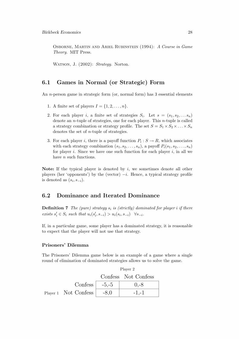
Prisoners’ Dilemma
The Prisoners’ Dilemma game below is an example of a game where a singleround of elimination of dominated strategies allows us to solve the game.
Player 2
Confess Not Confess
Confess -5,-5 0,-8
Player 1 Not Confess -8,0 -1,-1

Birkbeck Economics 29
How would you play this game?
In general there may be successive stages of elimination. This method of narrow-ing down the set of ways of playing the game is described as iterated dominance.If in some game, all strategies except one for each player can be eliminated onthe criterion of being dominated (possibly in an iterative manner), the game issaid to be dominance solvable.
Player 2
Left Middle Right
Top 4,3 2,7 0,4
Player 1 Middle 5,5 5,-1 -4,-2
Bottom 3,5 1,5 -1,6
We can eliminate dominated strategies iteratively as follows.
1. For player 1, Bottom is dominated by Top. Eliminate Bottom.
2. In the remaining game, for player 2, Right is dominated by Middle. Elim-inate Right.
3. In the remaining game, for player 1, Top is dominated by Middle. Elimi-nate Top.
4. In the remaining game, for player 2, Middle is dominated by Left. Elimi-nate Middle.
This gives us (Middle,Left) as the unique equilibrium.
6.3 Weak Dominance
Definition 8 The (pure) strategy si is weakly dominated for player i if thereexists s′i ∈ Si such that ui(s′i, s−i) ≥ ui(si, s−i) ∀s−i, with strict inequalityholding for some s−i.
Player 2
Left Right
Top 5,1 4,0
Player 1 Middle 6,0 3,1
Bottom 6,4 4,4
Here, for player 1, Middle and Top are weakly dominated by Bottom. EliminateMiddle and Top. The equilibria are (Bottom, Left) and (Bottom, Right).

Birkbeck Economics 30
6.4 Nash Equilibrium
However, for many games the above criteria of dominance or weak dominanceare unhelpful - none of the strategies of any player might be dominated orweakly dominated.
The following is the central solution concept in game theory.
Definition 9 (Nash Equilibrium in Pure Strategies) A strategy profile (s∗i , s∗−i)is a Nash equilibrium if for each player i,
ui(s∗i , s∗−i) ≥ ui(si, s
∗−i) ∀ si ∈ Si.
Player 2
Left Middle Right
Top 0,4 4,0 5,3
Player 1 Middle 4,0 0,4 5,3
Bottom 3,5 3,5 6,6
The only Nash Equilibrium in this game is (Bottom, Right).
A Nash equilibrium is a strategy combination in which each player chooses abest response to the strategies chosen by the other players. In the Prisoners’Dilemma, the case in which each prisoner confesses is a Nash equilibrium. (Ifthere is a dominant strategy equilibrium, it must be a Nash equilibrium aswell).
In general, we can argue that if there is an obvious way to play the game, thismust lead to a Nash equilibrium. Of course, there may exist more than oneNash equilibrium in the game, and hence the existence of a Nash equilibriumdoes not imply that there is an ‘obvious way to play the game’.
How to look for Nash Equilibria in simple games? Consider the following game,known as the “battle of the sexes.”
Wife
Football Opera
Football 2,1 -1,-1
Husband Opera -1,-1 1,2
In essence, we must examine all strategy combinations, and for each one, checkto see if the Nash equilibrium conditions are satisfied. Consider the Battle ofthe Sexes depicted in the figure above.
a. Start with the strategy combination (Football, Football).

Birkbeck Economics 31
(a1) Look at the payoffs from the husband’s viewpoint. If the wife goes to thefootball match, is football optimal for him? Yes, because 2 > −1.
(a2) Now look at the payoffs from the wife’s viewpoint. If the husband goes tothe football match, is football optimal for her? Yes, because 1 > −1.
Since the answer is ‘yes’ in both (a1) and (a2), (Football, Football) is a Nashequilibrium.
b. Next, consider the strategy combination (Football, Opera).
(b1) Look at the payoffs from the husband’s viewpoint. If the wife goes to theOpera, is football optimal for him? No, because by going to the football hegets -1, and he could do better by going along to the Opera which would fetch1. For this strategy combination, the Nash equilibrium condition does not holdfor the husband.
(b2) We could look at this strategy combination from the wife’s viewpoint, butgiven that the Nash condition does not hold in (b1), we need not really bother.
In short,(Football, Opera) is not a Nash equilibrium.
c. Next, consider the strategy combination (Opera, Opera)....
Checking (c1) and (c2), this turns out to be a Nash equilibrium.
d. Next, consider the strategy combination (Opera, Football) This is not aNash equilibrium.
In sum, there seem to be two Nash equilibria in this game, namely (Opera,Opera) and (Football, Football).
If the game had three strategies for each player, there would be 9 possiblestrategy combinations for us to check for Nash equilibria.
6.5 Nash Equilibrium in Mixed strategies
Some games do not seem to admit Nash equilibria in pure strategies. Considerthe game below called “matching-pennies.”
Player 2
Heads Tails
Heads 1,-1 -1,1
Player 1 Tails -1,1 1,-1
Notice that this game seems to have no Nash equilibria, at least in the sense thatthey have been described thus far. But, in fact it does have a Nash equilibriumin mixed strategies.
The first stage in the argument is to enlarge the strategy space by constructingprobability distributions over the strategy set Si.

Birkbeck Economics 32
Definition 10 (Mixed Strategy) A mixed strategy si is a probability distri-bution over the set of (pure) strategies.
In the matching pennies game, a pure strategy might be Heads. A mixedstrategy could be Heads with probability 1/3, and Tails with probability 2/3.Notice that a pure-strategy is only a special case of a mixed strategy. A Nashequilibrium can now be defined in the usual way but using mixed strategiesinstead of pure strategies.
Definition 11 (Nash Equilibrium) A mixed-strategy profile (σ∗i , σ−i) is a
Nash equilibrium if for each player i,
ui(σ∗i , σ
∗−i) ≥ ui(si, σ−i) ∀si ∈ Si.
The essential property of a mixed strategy Nash Equilibrium in a 2 player gameis that each player’s chosen probability distribution must make the other playerindifferent between the strategies he is randomizing over. In a n player game,the joint distribution implied by the choices of each player in every combinationof (n− 1) players must be such that the n-th player receives the same expectedpayoff from each of the strategies he plays with positive probability.
Once we include mixed strategy equilibria in the set of Nash Equilibria, we havethe following theorem.
Theorem 5 (Existence) Every finite-player, finite-strategy game has at leastone Nash equilibrium.
Clearly, if a game has no equilibrium in pure strategies, the use of mixed-strategies is very useful. However, even in games that do have one or more purestrategy Nash equilibria, there might be yet more equilibria in mixed-strategies.For instance, we could find a mixed-strategy Nash Equilibrium in the Battle ofthe Sexes.
6.6 Games in Extensive Form
The extensive form is particularly useful when the interaction is principallydynamic. It provides a clear description of, say, the order in which the playersmove, what their choices are, the information that each player has at each stageand so on. The extensive form is often represented by a game tree.
The description involves the following elements.
1. A finite set of players I = {1, 2, . . . , n}. In addition, there may be anadditional player to capture the uncertainty, called Nature (denoted byN).
Birkbeck Economics 33
2. A game tree consists of a set of nodes with a binary precedence relation-ship. Think of it as a configuration of nodes and branches. A node (moreaccurately, a decision node) represents a point at which a player (or ‘na-ture’) must choose an action. The choice of an action takes that playerdown a branch to a successor node. The idea of an initial node and termi-nal node(s) is obvious in this context. A game tree is a configuration ofnodes and branches running from the initial node to the terminal nodes,with the restriction that there be no closed loops in the tree.
3. One player or (nature) is assigned to each node. This is just a way ofspecifying which player must choose (take an action) at that node.
4. For each node, there is a finite set A of available actions, which lead tothe immediate successor nodes of that node.
5. Each players nodes are partitioned in to information sets, which measuresthe fineness of the information available to that player when s/he choosesan action. If two nodes lie in the same information set, the player knowsthat s/he is at one of those two nodes but does not know which one.
6. An assignment of payoffs, one for each player, at each terminal node.
7. A probability distribution over nature’s moves.
The notion of a strategy is fairly straightforward in a normal form game. How-ever, for an extensive form game, it is a little bit more complicated. To under-stand what a typical element of the strategy set Si for player i is, let h be atypical information set for player i, and A(h) the set of actions available at thatinformation set. A (pure) strategy for player i specifies which action she musttake at each of her information sets. The set of all strategies for that player isgiven as Si = ΠhA(h).
Note: It is very important to understand the distinction between actions andstrategies for an extensive form game. A strategy is a complete plan of actions.
Birkbeck Economics 34
6.7 Actions and Strategies
6.7.1 Game1
1
2
A B
L R
1 0
0 1
Payoff to 1Payoff to 2( )
( )( )1
L R
C D DC
0 0( ) 1
1( ) 0 0( ) 2
2( )
1
2
Game 1
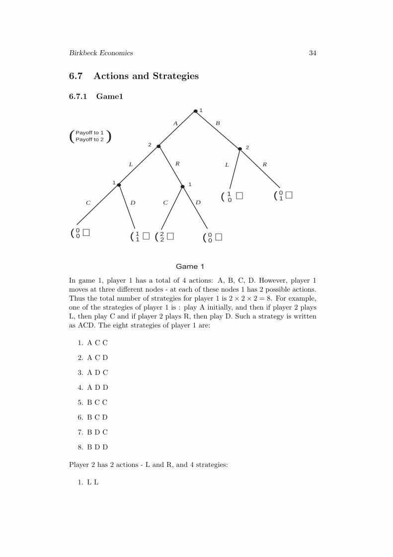
In game 1, player 1 has a total of 4 actions: A, B, C, D. However, player 1moves at three different nodes - at each of these nodes 1 has 2 possible actions.Thus the total number of strategies for player 1 is 2 × 2 × 2 = 8. For example,one of the strategies of player 1 is : play A initially, and then if player 2 playsL, then play C and if player 2 plays R, then play D. Such a strategy is writtenas ACD. The eight strategies of player 1 are:
1. A C C
2. A C D
3. A D C
4. A D D
5. B C C
6. B C D
7. B D C
8. B D D
Player 2 has 2 actions - L and R, and 4 strategies:
1. L L

Birkbeck Economics 35
2. L R
3. R L
4. R R
6.7.2 Game2
1
2
A B
L R
1 0
0 1
Payoff to 1Payoff to 2( )
( )( )1
L R
C D DC
0 0( ) 1
1( ) 0 0( ) 2
2( )
Game 2
In game 2, on the other hand, player 1 moves only at two different informationsets (each node is also a trivial information set). Thus 1 has only 4 strategies:AC, AD, BC, BD. Player 2 only moves at one information set - thus for 2, actionsand strategies coincide. Player 2 has only 2 actions as well as 2 strategies: Land R.
6.8 Analyzing Extensive Form Games
Now that we can write down the strategies for players, how do we identify theNash equilibria of such games? We do so by converting extensive form gamesto normal form games. To every extensive form game there is a correspondingstrategic form game. But a given strategic form game can, in general, corre-spond to several different extensive form games.
The normal form for game 2 is as follows:

Birkbeck Economics 36
Player 2
L R
AC 0,0 2,2
Player 1 AD 1,1 0,0
BC 1,0 0,1
BD 1,0 0,1
From this, it is easy to see that there are 2 pure strategy Nash equilibria: (AC,R) and (AD, L).
6.9 Equilibrium Refinement
The use of Nash equilibrium as a guide to the likely outcome of a game-theoreticsituation requires some justification. It is hard to convey the nuances in a briefguide but some remarks follow. First, one could argue that if there is a self-evident way to play the game, it must be a Nash equilibrium. Two, we couldview the Nash equilibrium as the ’outcome’ of preplay negotiation: if playerscarry out pre-play negotiation, we would like the agreed-to action to be self-enforcing in the sense that given that others will fulfill their part of the deal, itis in your interest to not deviate. Three, we can think of Nash equilibrium asthe outcome of evolution, or of learning.
Regarding the first one of these remarks, it suggests that being Nash is a nec-essary condition for a strategy combination to be a self-evident way to play thegame but may not be sufficient. In any game where the game-form admits morethan one equilibrium, we need other criteria to narrow down the equilibriumset. This procedure is described as refinement. The actual notions used torefine the set of equilibria are varied and do not all have universal acceptabilityin the discipline.
Weak Dominance We may choose to eliminate equilibria that involve theuse of weakly dominated strategies.
Subgame perfect equilibria (SPE), and the issue of credibility A sub-game is a game consisting of a node which is a singleton, that node’s successorsand the payoffs at the associated end-nodes.
A strategy combination is a subgame perfect equilibrium (SPE) if it is a NashEquilibrium (NE) for the entire game and the implied strategies for any subgameare a NE for that subgame. We will discuss some illustrative examples in thelecture. Here is a simple example:
Consider the following extensive form game.

Birkbeck Economics 37
2 Payoff to 1Payoff to 2( )
1
2 0( ) 1
1( ) 3 3( ) 0
2( )
Game 3
t n t n
2
T N
The normal form is given by
Player 2
tt nt tn nn
T 1,1 2,0 1,1 2,0
Player 1 N 0,2 0,2 3,3 3,3
Thus there are 3 pure strategy Nash Equilibria: (T,tt), (N,nn), (N,tn).
However, in the subgame on the left hand side, the (trivial) Nash equilibrium(in this subgame only one player plays - so 2’s optimal strategy in the subgameis trivially the Nash equilibrium for the subgame) is ‘t’. In the subgame on theright hand side, the Nash equilibrium is ‘n’. Thus the only Nash equilibriumthat induces Nash equilibria in all subgames is (N,tn) - this is therefore the onlysubgame perfect Nash equilibrium.
The issue of subgame perfection is closely linked to those of credible threatsand of credible promises. Very crudely speaking, consider a Nash equilibriumwhich is not subgame perfect. That implies there must be a subgame such thatthe strategy over that remaining subgame is not a Nash equilibrium for thatsubgame. So if by chance we end up at that sub game, we do not expect thatthe players will find it profitable to stick to that ’portion’ of the strategy: if not,that portion of the strategy is not credible. The issue is best discussed throughsome examples such as entry deterrence, credibility of government policy etc.
Other Refinements There are other kinds of refinements that result in, say,sequential equilibria, trembling-hand perfection, etc. but constraints of timewill prevent us from exploring these in any detail. Those interested in these areadvised to read more extensively in these areas.
Birkbeck Economics 38
6.10 Games of Incomplete Information
We have implicitly assumed that (for the extensive form) the players know whatthe game-tree looks like, they know that the other players know what the gametree looks like, and so on. This recursion is formalized as common knowledge.
Definition 12 (Common Knowledge) Information is common knowledge ifit is known to all players, each player knows that they all know it, each of themknows that all of them know that all of them know it, and so on.
The players might or might not have full information about all aspects of agame that they are about to play. Below we consider the possibilities.
Perfect information There is no uncertainty arising from moves of nature.When such uncertainties exist, the situation is one of imperfect information.
Complete information All players know all the relevant information abouteach other, including payoffs that each receives from various outcomes. Whenthis is not the case, so that players might not know about others’ payoffs. Thiscreates a problem in analyzing the game. We now need to know about a player’sbeliefs about other players preferences, his beliefs about the beliefs of othersabout his preferences, his beliefs about the beliefs of others about his beliefsand so on. This complicates the situation thoroughly.
However, we do have an approach that avoids this problem. This was thecontribution of Harsanyi (one of the three economists who won the Nobel Prizefor their work in Game Theory in 1994 - the other two were Nash and Selten).In this approach, it is assumed that each player’s preferences are determined bythe realization of a random variable. The actual realization is known to onlythe player in question, but the distribution of the random variable is commonknowledge. The random variable for a player is labelled his “type.” Since thedistribution of each players types are common knowledge, the game becomesexactly like a game of imperfect information where nature makes the first moveand chooses realizations of types (each player observes the realization of onlyhis own type). A game with this structure is called a Bayesian game.
What is an equilibrium of such a game? A Bayesian Nash equilibrium is a Nashequilibrium of this imperfect information game. It is a set of (type-contingent)strategies such that each player maximizes his expected utility, contingent onher type, and taking the other player’s type-contingent strategies as given.
6.11 Repeated Games and the Folk Theorem
Suppose a particular game such as the ‘Prisoners’ Dilemma’ is played a largenumber of times. Can we say something about the behaviour of players in such‘supergames’ that is not obvious in the analysis of the one-shot game?

Birkbeck Economics 39
To anticipate the argument, we will try and establish that if the game is repeateda large number of times, we cannot rule out some outcomes that are clearlyunlikely in case the game was played just once.
First, we need to have an appropriate notion of payoffs in the supergame, ormore accurately, the relationship between the payoff in the supergame and inthe one-shot constituent game (now called the stage game). The average payoffover the supergame is some aggregate measure of the payoffs from the stagegames, with later payoffs possibly discounted for the lag with which they willbecome available.
The ‘folk theorems’ for repeated games are usually some variant of a simple idea,namely that, if the players are sufficiently patient, then any feasible, individuallyrational payoff combination can be supported as a Nash equilibrium (the twoadjectives need some explanation). One conclusion that emerges from this isthat outcomes that were ruled out in the one-shot game (eg. cooperation inthe Prisoners’ Dilemma) can be ’sustained’ in the associated repeated game.The intuition for this might run as follows: if players deviate from say, anagreement to cooperate they could be punished by the other(s) in subsequentrounds which would cause loss of utility in every subsequent period. (Howhard they can be punished depends on what their reservation utility is; howcostly this future punishment seems to them depends on their discount factor).Fearing this reduction of utility in later rounds (which would reduce the averagepayoff) breeds compliance or cooperation. This has considerable application inmodels of say, lender-debtor interaction, product quality, entry deterrence, etc.
This idea is quite useful in understanding why cooperation is sustained in thereal world.
6.12 Some game-theoretic models of oligopoly
We now apply some of the techniques developed so far to model the oligopolisticinteraction between firms. Since the aim here is to see how notions such as Nashequilibrium relate to oligopoly, the details of the underlying market are keptas simple as possible. For instance, we readily assume that firms are identical,demand curves are conveniently linear, and so on. More general versions of theexamples presented here can easily be generated.
6.13 Bertrand Equilibrium: Nash equilibrium in prices
We first consider a case with two identical firms, each producing the same homo-geneous product. Production is costless. The firms face a standard downward-sloping demand curve, and their individual share of the total market demanddepends on the combination of prices charged by them. Put simply, the firmwith the lower price captures the entire market; if they charge the same price,they get half the market each. The prices are chosen ’simultaneously’. Let ussee how we can model this as a game.

Birkbeck Economics 40
Label the firms as firm 1 and 2. The strategy set for each firm can be thoughtof as the set of non-negative prices, p. The payoff function measures the profitmade by a firm for any given strategy combination. This can be written asπi(pi, pj), for i = 1, 2 and j �= i. In this case,
π1(p1, p2) = p1q1
where
q1 =
q if p1 < p2
0 if p1 > p2
q/2 if p1 = p2.
Firm 2’s payoff function is defined symmetrically, π2(p1, p2) = p2q2. Here aNash equilibrium is a pair of prices (p∗1, p∗2) such that
1. π1(p∗1, p∗2) ≥ π1(p1, p∗2) ∀p1, and
2. π2(p∗1, p∗2) ≥ π1(p∗1, p2) ∀p2.
How do we compute the equilibrium? That is, how do we find the prices thatsatisfy conditions 1 and 2? Let us look at some candidate solutions.
Case 1 p∗1 > p∗2 > 0.
Does this satisfy 1 and 2? At this configuration of prices, π1 = 0 andπ2 > 0. (Why?) If firm 1 had chosen some other price, say p∗2− ε, it couldhave captured the entire market. Hence the solution could not be of thisform.
Case 2 p∗1 = p∗2 > 0.
This, too, is not an equilibrium. Either firm, if it had chosen a lowerprice, could have captured a much larger share of the market and madehigher profits. (Why?)
Case 3 p∗1 > p∗2 = 0.
This cannot be an equilibrium because firm 2 could have charged a slightlyhigher price without losing its market share and made strictly greaterprofits.
By the process of elimination, we reach the conclusion that the unique Nashequilibrium is given by
p∗1 = p∗2 = 0.
The paradoxical feature of this solution is that, in equilibrium, the firms makeno (super-normal) profits. This seems unrealistic.
As an exercise comment on the outcome in the above game if each firm producesat positive, but constant, marginal cost c. What if the marginal cost is not thesame for the two firms?

Birkbeck Economics 41
6.14 Cournot equilibrium: Nash equilibrium in quan-
tities
Assume, as in the previous example, that there are two identical firms produc-ing costlessly but now suppose the firms choose, not prices, but quantities tosupply to the market. Assuming that the market clears, each firm obtains themarket clearing price for each unit of the good supplied. To obtain the payoff-function we now need to incorporate the market demand function explicitly.For algebraic simplicity, we use a very simple demand function,
q = 120 − p.
Let q1 and q2 be the output levels supplied by firm 1 and 2, respectively. Themarket clearing condition amounts to q1 + q2 = q. For any given strategy-combination (q1, q2) the market price is p = 120 − (q1 + q2). Therefore, thepayoff-function (profits) for firm 1 is given as
π1(q1, q2) = pq1 = (120 − q1 − q2)q1
and likewise for firm 2.
A Nash equilibrium is defined in the usual way: it is a pair of strategies (namely,quantity choices) (q∗1, q∗2) such that
1. π1(q∗1, q∗2) ≥ π1(q1, q∗2) ∀q1, and
2. π2(q∗1, q∗2) ≥ π1(q∗1, q2) ∀q2.
Since in this case the payoff functions are differentiable in the strategy variable,we can obtain the Nash equilibrium by the standard optimization techniques.
First, compute the profit maximizing output choice for each firm taking therival’s output as parametric. Setting
∂π1
∂q1= 0
we get, q1 = 60− .5q2. This is the “reaction function” for firm 1. Similarly, wecan obtain a reaction function for firm 2, q2 = 60 − .5q1.
We then ’solve’ the two reaction functions to obtain the Cournot-Nash solution.For this example, it turns out to be q∗1 = q∗2 = 40.
As an exercise generalize the above for the case where the are n firms.
6.15 Duopoly with sequential moves: the Stackel-
berg equilibrium
Suppose the choice variable is output level as in the Cournot case but the choicesare made sequentially. Firm 1 (the ‘leader’) chooses its output level before firm

Birkbeck Economics 42
2 (the ‘follower’) does, and the follower can observe the leader’s choice beforeshe makes her output choice. It is not hard to see that the follower’s reactionfunction is as in the previous example but the leader now optimizes taking thefollower’s reaction function (rather than output level) as given. In other words,the leader maximizes
π1(q1, q2) = pq1 = (120 − q1 − (60 − .5q1))q1.
The Nash equilibrium of this game, also known as the Stackelberg equilibrium,is here given by q∗1 = 60, q∗2 = 40.
Chapter 7
Topics in Information Economics: Adverse Selection
1. The adverse selection problem.
2. Akerlof’s application to the second-hand car market.
3. Adverse selection under common values - contracts in insurance markets.
4. Adverse selection - a general model.
5. Adverse selection, debt contracts and credit rationing.
6. Signaling
Readings
1. Salanie, B. (1997) The Economics of Contracts, ch 2.
2. Wolfstetter, D. (1999) Topics in Microeconomics, ch 9-10.
3. Jehle & Reny, ibid, ch 10
4. Akerlof, G. (1970): “The Market for Lemons,” Quarterly Journal ofEconomics, 89, 488-500.
5. Spence, M. (1973): “Job Market Signaling,” Quarterly Journal of Eco-nomics, 87, 355-374.
6. Stiglitz, J., and A. Weiss (1981): “Credit Rationing in Markets withImperfect Information,” American Economic Review, 71, 393-410.
7. Rothschild, M., and J. Stiglitz (1976): “Equilibrium in competi-tive insurance markets,” Quarterly Journal of Economics, 90, 629-649.
43

Birkbeck Economics 44
7.1 Introduction
For a wide range of products (for example, things you buy from a grocery storeor a drug store) the markets are large and decentralized, and the exchanges areanonymous. Usually you do not know who owns the grocery store when you goin to buy a tube of toothpaste or a zucchini, nor does the owner bother to keeptrack of every customer.
There are, however, important exceptions. Consider the market for used cars.It is difficult to tell how good or bad a used car is unless you use it for sometime. The seller, on the other hand, knows how good the car is.
In such situations, you would care about the identity of the seller. In fact, insuch cases anonymous exchange is often impossible, as that would lead to abreakdown of the market. The customers are willing to pay a price based onthe average quality. However, this price is not acceptable to the better thanaverage quality car owner. This leads the owners of better than average carsto leave the market. But the same phenomenon then applies to the rest of themarket, and so on.
The problem is called “lemons problem” or “adverse selection.”
The same problem arises in selling insurance. The insurance company mustknow the customer and her past record of illnesses. Anonymous exchange would,in general, lead to a market price (in this case insurance premium) that is toohigh - and only the people who feel that they are very likely to claim theinsurance would buy insurance. This would lead, as in the case of used carsabove, the market to fail.
A different sort of problem arises when you, as the manager of a company,are trying to hire some salespeople. As the job requires a door to door salescampaign, you cannot supervise them directly. And if the workers choose not towork very hard, they can always blame it on the mood of the customers. If youpay them a market clearing flat wage, they would (assuming away saintliness)not work hard.
This problem is known as “moral hazard.”
Note the difference between adverse selection and moral hazard. In the firstcase, the asymmetry in information exists before you enter into the exchange(buy used car, sell insurance). In the latter, however, the asymmetry in infor-mation arises after the wage contract is signed.
This is why another name for adverse selection is “hidden information” andanother name for moral hazard is “hidden action.”
In the following sections, we will consider certain remedies to adverse selectionand moral hazard. In what follows, attitudes towards risk will play a role.
First, a fuller description of the lemons problem. This was first noted by Akerlof(1970). At the time, hardly anyone understood the importance of his ideas. Fivetop journals rejected his paper. Today, of course, it is recognized as a classic. Ithas spawned a huge literature on information economics that has significantlyadvanced our knowledge of economic institutions.

Birkbeck Economics 45
7.2 Akerlof’s Model of the Automobile Market
Suppose there are four kinds of cars — there are new cars and old cars, and ineach of these two categories there may be good cars and bad cars. Buyers ofnew cars purchase them without knowing whether they are good or bad, butbelieve that with probability x they will get a good car, and with the residualprobability (1 − x), a bad car.
After using a car for some time the owners can find out whether the car is good.This leads to an asymmetry: sellers of used cars have more information aboutthe quality of the specific car they offer for sale. But good cars and bad carsmust sell at the same price — since it is impossible for the buyer to differentiate.
It is obvious that a used car cannot have the same valuation as a new car.(why?) Further, the owner of a good used car must be locked in. Bad carsdrive out good cars. Analogy with Gresham’s Law.
A Generalization to the case with continuous grades of quality Thiscase may prove to be more pathological. Suppose we can index quality by somenumber q which is uniformly distributed in the interval [0,1]. Hence the averagequality of the cars is 1/2. Suppose that there are a large number of buyers whoare prepared to pay 3q/2 for a car of quality q, and sellers are prepared to sella car of quality q at price q. Therefore, if quality was an observable attribute,any price in this range would be admissible.
If quality of an individual car cannot be observed by the buyers, they will basetheir decisions on the average quality of the cars in the market — this maybe observable. If the average quality is given by Q, then the buyers should beready to pay 3Q/2. What is the likely outcome in this market? If the pricewere p, all sellers with cars of quality less than p will offer their cars for sale.Hence, average quality of the cars that appear in the market will be Q = p/2.Hence the reservation price of the buyers will be 3Q/2 = 3p/4. In other words,we can think of no price at which the buyers will be prepared to pay the askingprice, and the market has been ’driven down’ altogether.
Implications This is an instance of market failure owing to adverse selection,and if the welfare gains from trade in the market are sufficiently great, there maybe gains from government intervention. Or, alternatively there may be scopefor private institutions to evolve in such markets which serve as guarantors ofquality. Of course, it is costly to set up these institutions, but these costs maybe more than made up by the gains from trade in the relevant market.
Standard applications of this model include the medical insurance markets (oldpeople cannot buy insurance at any price), the cost of dishonesty, credit marketsetc. It is also interesting in this context to think of the specific institutions setup to counteract these problems.

Birkbeck Economics 46
7.3 Adverse Selection and Contracts
7.3.1 Adverse Selection: Description of the Problem
There are two states of the world - a state in which a loss (fire, accident, injury)occurs and one in which a loss does not occur. We will denote the former by Land the latter by NL. The dollar value of the loss is L.
There are two types of people. Good (G) and bad (B). The names reflect thefact that a good type person has a lower probability of being in the loss statethan a bad type. Both types have initial wealth (or income) W . Thus incomeis W − L in the loss state and W otherwise.
For a G-type, probability of L is p and the probability of NL is (1 − p). For aB-type, the probability of L is q and the probability of NL is (1 − q). By thedefinition of the two types, p < q.
Contract
A contract is a pair (C, R) where C is a compensation paid by the insurancecompany to the insuree if the loss (which has a money value of L dollars) occur.R is the premium paid by the insuree to the insurance company in every stateof the world.
The Payoffs
We will assume, for simplicity, that the insurance sector is competitive, and thusthe insurance company makes a zero profit in equilibrium. We will also assumethat the insurance company is risk neutral and cares only about expected value.
Thus the payoff of the insurance company from a contract (C, R) is given by
Prob(L)(−C + R) + Prob(NL)R
The insurees are risk averse (indeed, otherwise there would not be much of ademand for insurance!). They maximize their expected utility.
The expected utility of a G-type when he does not have any insurance is givenby
pu(W − L) + (1 − p)u(W )
His expected utility if he signs a contract (C, R) is given by
pu(W − L + C − R) + (1 − p)u(W − R)
Similarly, for a B-type, expected utility without insurance is given by
qu(W − L) + (1 − q)u(W )

Birkbeck Economics 47
and his expected utility with insurance of (C, R) is given by
qu(W − L + C − R) + (1 − q)u(W − R)
Note that any feasible insurance contract must have C > R (otherwise nobodywill ever accept an insurance contract).
The adverse selection problem is that the insurance company cannot distinguishbetween types. But first, let us consider the outcome if the insurance companycould distinguish. This will provide a benchmark for deciding the importanceof the information problem.
7.3.2 First Best: No Information Problem
Before we discuss how contracts can address the adverse selection problem, letus discuss the case where the insurance company faces no information problem,i.e. they know the type of each customer.
In this case, the insurance company will offer two contracts - one for each type.Let us denote the contract for the good type by (Cg, Rg) and the contract forthe bad type by (Cb, Rb).
Since people dislike risk, and the insurance company is neutral to risk, theoptimal involves the insurance company absorbing all the risk and leaving theinsurees with a sure income. Another way of saying the same thing is that inthe first best situation, the insurance company will provide full insurance.
Full insurance for the good type implies:
W − L + Cg − Rg = W − Rg
=⇒ Cg = L (7.1)
Thus the compensation covers the loss fully. What about the premium? Well,that depends on the division of the surplus between the insuree and the in-surance company. But we have already assumed that the insurance companybelongs to a competitive sector and hence earns 0 profits. Thus we have
Prob(L)(−Cg + Rg) + Prob(NL)Rg = 0 (7.2)
But since we are talking about the G-type, the relevant probabilities are p and(1 − p). Thus,
p(−Cg + Rg) + (1 − p)Rg = 0 (7.3)
which impliesRg = pCg = pL (7.4)
Denoting the first best variables by a superscript ∗, we have
C∗g = L (7.5)
R∗g = pL (7.6)

Birkbeck Economics 48
For the bad type, the problem is the same, the only difference is in the proba-bilities. Thus we have,
C∗b = L (7.7)
R∗b = qL (7.8)
So the first best involves full coverage (or full insurance) for both types anda premium equal to the expected value of the loss for each type. Thus thepremium is higher for the bad type.
Another way of saying this is as follows: Note that the net amount received bya good type if the loss occurs is L − pL = (1 − p)L. If no loss occurs, he paysout pL. Thus he is effectively buying an extra income of (1 − p)L in the lossstate by paying out pL in the no loss state. Thus the price of an extra dollar ofincome in the loss state is p/(1 − p) dollars of income in the no loss state. Thusa good type can transfer income from the no loss state to the loss state at aprice of p/(1 − p).
Similarly, a bad type can transfer income from the no loss state to the loss stateat a price of q/(1 − q).
These are called “actuarially fair” prices (the insurance company is taking ona fair bet because their expected gain is zero).
7.3.3 Saying It with a Picture
Let IL denote the income in the loss state and IN denote the income in theno-loss state. An indifference curve of a G-type is given by
pu(IL) + (1 − p)u(IN ) = u0
for some constant u0. The slope of the indifference curve is
dIL
dIN= −
(1 − p
p
)u′(IN )u′(IL)
(7.9)
Since full insurance implies IL = IN , we have,
dIL
dIN
]at full ins.
= −(
1 − p
p
)(7.10)
This, then, is the slope of the indifference curve at the point where it intersectsthe 45◦ line, as that is the line of full insurance.
Let πL and πN denote the payoff of the insurance company in the loss stateand the no loss state respectively. A zero profit (for the insurance company)line for a contract for the good types is given by
pπL + (1 − p)πN = 0 (7.11)
Thus the slope of a zero-profit-from-good-type-contract is given by
dπL
dπN= −
(1 − p
p
)(7.12)

Birkbeck Economics 49
Indiff-B
Indiff-G
45o
(W,W-L)
G*
B*
line ofzero-profitfrom B-type
line ofzero-profitfrom G-type
[Full Insurance line]IL
IN
Figure 1: First best. B* is the first best contract for type Band G* is the first best contract for type G. The dashed curvesare the original (e.g. before buying insurance) indifference curves.
O
Birkbeck Economics 50
Thus the indifference curve of a good type person is tangent to the zero-profitline along the 45◦ line.
A similar condition, with q instead of p, holds for a bad type. Note that
1 − p
p>
1 − q
q
as q > p. Thus the indifference curves for the good types are steeper than thatof the bad types. The same goes for the zero profit lines. The zero-profit linefor a good type contract is steeper than that of a bad type contract.
Figure 1 shows these properties, and shows the first best solution.
7.3.4 A Separating Solution
Now suppose that the insurance company cannot tell the two types apart. So ifthey want to offer two different contracts, all they can do is offer both contractsto any customer and let him or her choose the contract that he or she wants.
So if they now offer two different contracts, they should make sure that eachtype has the incentive to pick the contract for his own type. This is called theincentive compatibility constraint.
Note that the first best contracts violate incentive compatibility. If they areoffered, all types will take the contract (C∗
g , R∗g) as both contracts have the
same coverage (C∗g = C∗
b = L), but the contract for the good type has a lowerpremium (or, equivalently, a lower price), as R∗
g = pL < qL = R∗b .
Suppose the insurance company offers two contracts (Cg, Rg) and (Cb, Rb). In-centive compatibility requires that the bad types do not take the contract forthe good type (we will see that a good type will never want to take the contractfor the bad types).
Thus the incentive compatibility constraint (ICC) is given by:
qu(W−L+Cb−Rb)+(1−q)u(W−Rb) ≥ qu(W−L+Cg−Rg)+(1−q)u(W−Rg)(7.13)
Note that by claiming to be a good type, a bad type person can obtain thecontract meant for the good type, but he cannot change his inherent probabilityof being in a loss state. This is why the probabilities on the right hand side(which shows the utility associated with taking the contract (Cg, Rg)) are stillq and (1 − q). The left hand side shows the utility associated with taking thecontract (Cb, Rb).
We will assume that if so long as the above constraint holds with equality, thebad types will choose (Cb, Rb) and not (Cg, Rg).
So we need to see what the best contracts are subject to the incentive com-patibility constraint and the zero-expected-profit condition for the insurancecompany.
Since we are concerned about the B-types taking the contract meant for the G-types, we should start by giving the B-types the best possible contract subjectto the constraint that the insurance company makes zero profits.

Birkbeck Economics 51
The best such contract, obviously, is the first best contract for the B-types.Thus we should offer the B-types the following contract:
Cb = L, Rb = qL
In order to design the contract for the good type, we need to take into accountthe incentive compatibility constraint. If we make the contract too attractive,the bad types will switch over. Basically, (Cg, Rg) must be such that
qu(W−L+Cg−Rg)+(1−q)u(W−Rg) = qu(W−L+Cb−Rb)+(1−q)u(W−Rb)(7.14)
Substituting the values of Cb and Rb on the right hand side, we get qu(W−qL)+(1− q)u(W − qL) = u(W − qL). Thus the incentive compatibility constraint is
qu(W − L + Cg − Rg) + (1 − q)u(W − Rg) = u(W − qL) (7.15)
Also, the zero profit condition for the insurance company is given by
p(Rg − Cg) + (1 − p)Rg = 0
which can be rewritten asRg = pCg (7.16)
Thus equations (7.15) and (7.16) determine Cg and Rg. Substituting equa-tion (7.16) in equation (7.15), we get
qu(W − L + (1 − p)Cg) + (1 − q)u(W − pCg) = u(W − qL) (7.17)
First let us show that the good types cannot be given full insurance. Fullinsurance implies
W − L + (1 − p)Cg = W − pCg
which, in turn implies L = Cg. But with L = Cg, the right hand side of theequation above becomes u(W − pL), which is greater than the left hand side.The same would be true if Cg > L. Thus we must have Cg < L.
Thus because of the presence of the bad types, the good types cannot be givenfull insurance and must bear some risk.
Finally, to check that the good types have no incentive to take the contract ofthe bad types, note that
u(W − qL) = qu(W − L + (1 − p)Cg) + (1 − q)u(W − pCg)< pu(W − L + (1 − p)Cg) + (1 − p)u(W − pCg)
where the last expression on the right hand side is the utility that the goodtype gets from taking its own contract.
(This last bit of checking was not really necessary - the fact that the good typewill not take the bad type contract is obvious, if you think about it.)
Thus we have found our best contracts subject to the incentive compatibilityconstraint. These are second best contracts.

Birkbeck Economics 52
Denoting the second best variables by a hat, we have
Cb = L (7.18)Rb = qL (7.19)
and
Cg < L (7.20)Rg = pCg (7.21)
where the precise value of Cg is given by the solution to
qu(W − L + (1 − p)Cg) + (1 − q)u(W − pCg) = u(W − qL) (7.22)
Figure 2 shows the separating equilibrium.
7.3.5 A Pooling Solution
Suppose the insurance company knew the fraction of the good and bad typesin the population. Then it could offer a single contract to both types.
Suppose that a fraction α are good types. Then a contract (C, R) that is offeredto both types would earn an expected profit of:
α(p(−C + R) + (1 − p)R) + (1 − α)(q(−C + R) + (1 − q)R)
which is equal toα(R − pC) + (1 − α)(R − qC)
equal toR − (αp + (1 − α)q)C
From the zero profit condition,
R − θC = 0 (7.23)
whereθ = αp + (1 − α)q (7.24)
is the average probability of the loss state.
Thus the best pooling contract would be to offer full coverage and ask forthe “average” premium from everybody. Thus the optimal pooling contract(Cp∗ , Rp∗) is
Cp∗ = L (7.25)Rp∗ = θL (7.26)
where θ is given by equation (7.24).
Note that θ is less than q (indeed, it is the average of q and p). Thus the badtypes would prefer to have the pooling contract over the separating contract.For the good types, the conclusion is not clear. If α is very high, they wouldvery likely prefer the pooling contract. If α is low, they would very likely preferthe separating contract. The exercises will be more explicit.
Figure 3 shows the pooling equilibrium.

Birkbeck Economics 53
Indiff-B
Indiff-G
45o
(W,W-L)
B
line ofzero-profitfrom B-type
line ofzero-profitfrom G-type
[Full Insurance line]IL
INO
^
G^
G*
Figure 2: Separating equilibrium.. Under adverse selection, the good types cannot be offered G* any more, as the bad types wouldalso ask for G*.
The best that can be offered to the good types is G, which is at the intersection of the zero-profit line for the G-types and the indifference curve of the B-types through B (which is the same as B*).For the G-types, G is clearly worse than G*. ^
^
^

Birkbeck Economics 54
Indiff-B
Indiff-G
45o
(W,W-L)
Slope = -(1-p)/p
[Full Insurance line]IL
INO
Slope = -(1-q)/q
Slope = -(1-θ)/θ
Figure 3: Pooling equilibrium.
q = a p + (1-a) q
where a is the proportion of G-types in the population, and (1-a) is the proportion of B-types in the population.
Birkbeck Economics 55
7.3.6 Existence of Separating and Pooling Solutions With Mul-
tiple Insurers
The above analysis assumes implicitly that there is only one insurance company.If there are more than one such companies competing with each other, one mustcheck whether the solutions offered above continue to be equilibria.
A pooling solution does not exist. To see this, note that a second insurercan enter the market and offer a contract anywhere in the shaded region infigure 4 (C, for example). This new contract attracts all the good types andnone of the bad types. Since the new contract is below the line of zero-profitfrom G-type, it earns a strictly positive profit. Thus indeed profitable entry ispossible which breaks the pooling solution. Thus the pooling solution cannotbe an equilibrium.
A separating solution might not exist. Let “pooling line” denote the lineof zero-profit from the entire population (this is, of course, the line with slope−(1 − θ)/θ). Suppose the population has a high proportion of G-types so thatthe pooling line (which is now close to the line of zero-profits from G-types)intersects the indifference curve of G-types passing through G (the good-typescontract in a separating equilibrium). Now any new contract such as C inthe shaded region (see figure 5) attracts both types and since it is below thepooling line, earns a strictly positive profit. Thus whenever the proportion ofgood types in the population is higher than a critical level (given by the level atwhich the pooling line is tangent to -i.e. just touches - the indifference curve ofgood types through G). A separating solution exists whenever the proportionof good-types in the population is below this critical level.

Birkbeck Economics 56
Indiff-B
Indiff-G
45o
(W,W-L)
Slope = -(1-p)/p
[Full Insurance line]IL
INO
Slope = -(1-q)/q
Slope = -(1-θ)/θ
Figure 4: Breaking a Pooling equilibrium.
C^

Birkbeck Economics 57
Slope = -(1-p)/p
IL
INO
Pooling Line(Slope = -(1-θ)/θ)
Figure 5: Breaking a separating equilibrium.
45o
(W,W-L)
B
line ofzero-profitfrom B-type
line ofzero-profitfrom G-type [Full Insurance line]
^
G^
C~

Birkbeck Economics 58
7.4 Signaling
What is a signal? When is a signal a signal? Market signals are activi-ties/attributes of individuals in a market that convey information to otherparticipants in the market. For example, advertising, brand-names or evenprices.
Spence’s model of job-market market signaling Suppose there are twotypes of workers, with productivity σ1 and σ2, with σ1 < σ2. The firm cannotdistinguish between the two types of workers. It could either offer them thesame average wage. Alternatively, it might be able to condition on some signal.Suppose more efficient workers can acquire information ’more cheaply’. Let thecost of acquiring one unit of education be c1 and c2, respectively, with c1 > c2.Suppose also that education has no effect on productivity
A separating equilibrium will require the education level contingent wage rateto be, s(a1) = w1 and s(a2) = w2 such that,
s(a1) − c1a1 ≥ s(a2) − c1a2,
ands(a2) − c2a2 ≥ s(a1) − c2a1.
Since there exists an a∗ such that
σ2 − σ1
c2> a∗ >
σ2 − σ1
c1,
a wage schedule such that s(a) = σ1 if a < a∗ and s(a) = σ2 if a > a∗, satisfiesthe self selection constraints.
Chapter 8
Topics in Information Economics: Moral Hazard
1. The principal-agent problem, moral hazard.
2. Risk neutral agents.
3. Risk averse agents and agency costs.
Readings
1. Jehle & Reny, ibid, ch 10
2. Holmstrom, B. (1979): “Moral Hazard and Observability,” Bell Jour-nal of Economics, 10, 74-91.
8.1 Introduction
Suppose a risk-averse individual has purchased an insurance policy that promisesto compensate her fully in case his bike is stolen. Once insured, the individualhas no incentive to be careful about securing the bike because if it is stolen,the insurance company, and not he, will bear the loss. (Assume, for the sake ofargument, that he does not mind the bother of reporting the loss to the police,filling claim-forms, etc.). Indeed, if being security-minded causes disutility, hemight choose to be downright careless, and so expose the insurance company toan especially high level of risk. Of course, the insurance contract may requirethat he take ‘due care’ to prevent theft, but then it may be hard to observecarelessness, or to prove it in a court of law. This phenomenon – that the veryact of insurance blunts the incentives of the insured party to be careful, and soincreases the overall risk to the insurer – is described as moral hazard in theinsurance literature.
We know how insurance companies react to this hazard. To preserve the rightincentives, they may provide only partial insurance. This exposes the insuredparty to at least some residual risk, and thus prompts more careful behavior.This feature of insurance contracts, namely that the risk is effectively sharedbetween the insurance company and the insured party is known as co-insurance.
59

Birkbeck Economics 60
Note that the consequence of the moral hazard problem is to reduce the amountof insurance that is available to individuals.
The moral hazard problem is a direct consequence of an informational asym-metry: in the example, the true level of care (or effort) is hidden from the firm.The asymmetry in information here is described as hidden action, as distinctfrom that of hidden type.
The issue can be studied more generally as a principal-agent problem. Manyeconomic transactions have the feature that unobservable actions of one indi-vidual have direct consequences for another, and the affected party may seek toinfluence behavior through a contract with the right incentives. In the aboveexample, the insurance company (the principal) is affected by the unobservablecarelessness of the insured (the agent): it then chooses a contract with onlypartial insurance to preserve the right incentives. Other economic relationshipsof this type include, shareholders and managers, manager and salespersons,landlord and tenants, patient and doctors, etc. We consider the principal-agentproblem a bit more generally.
8.2 A formalization
A principal (or just P ) hires an agent (A) to carry out a particular project.Once hired, A chooses an effort level, and his choice affects the outcome of theproject in a probabilistic sense: higher effort leads to a probability of success,and that translates into higher expected profit for P . If the choice of effort wasobservable P could stipulate, as part of the contract, the level of effort thatis optimal for her (that is, for P ). When effort cannot be monitored, P mayyet be able to induce a desired effort level, by using a wage contract with theright incentive structure. What should these contracts look like? The formalstructure can be set up as follows:
1. Let e denote the effort exerted by the agent on the project. Assume, forthe moment, that A can either work hard (choose e = eH) or take it easy(choose e = eL); the story can later be generalized for more than two, butfinite number of, effort choices. The choice of e cannot be monitored by P :this feature – hidden action – characterizes the informational asymmetryin the problem.
2. Let the random variable π denote the (observable) profit of the project.Profit is affected by the effort level chosen, but is not fully determined byit. (If it was fully determined, the principal can infer the true effort choicesby observing the realization of π: we would no longer be in a situationof hidden actions.) Higher effort leads to higher profit in a probabilisticsense. Assume that π can take a value in some finite set, {πi}. Letf(π|e) be the conditional probability of π under effort e, and F (π|e) bethe associated cumulative distribution. We assume that the distributionof π conditional on eH dominates (in the first order stochastic sense) the

Birkbeck Economics 61
distribution conditional on eL: we have F (π|eH) ≤ F (π|eL), with strictinequality for some π.
3. The principal is risk neutral: she maximizes expected profit net of anywage payments to the agent.
4. The agent is (weakly) risk-averse in wage-income, and dislikes effort. Hisutility function takes the form
u(w, e) = v(w) − g(e),
where w is wage received from the principal, and g(e) is the disutility ofeffort. Assume v′ > 0, v′′ ≤ 0, and g(eH) > g(eL).
Note the central conflict of interest here. The principal would like the agentto choose higher effort, since this leads to higher expected profits. But, otherthings being the same, the agent prefers low effort. However, (to anticipate ourconclusion), if the compensation w package is carefully designed, their inter-ests could be more closely aligned. For instance, if the agent’s compensationincreases with profitability (say, by means of a profit-related bonus), the agentwould be tempted to work hard (because high effort will increase the relativelikelihood of more profitable outcomes). However, this will also make the agent’scompensation variable (risky), and that is not so efficient from a risk-sharingperspective. The inefficiency in risk-sharing will be an unavoidable consequenceof asymmetric information.
5. The principal chooses a wage schedule w(π) that depends on π. Notethis is a (variable) payment schedule rather than a constant payment,precisely because the principal may wish to influence the effort choices ofthe agent. (More generally, the wage schedule could condition paymentsjointly on π and any other observable signal m that is correlated with theeffort choice.
With the right wage schedule, it may be possible to induce a particular effortchoice. To persuade the agent to accept the contract and to induce eH , forinstance, the wage contract must satisfy the following constraints:
• The contract should be acceptable to the agent. Let u0 be the reservationutility (the expected utility the agent gets from alternative occupations).The compensation package should be such that its expected utility undereH is at least as large as u0. This is the participation constraint (PC), orthe individual rationality constraint.
• The compensation package should be such that the agent prefers to exerteH rather than any other effort level. In other words, w(π) must createthe right incentives for choosing eH over eL. This is called the incentivecompatibility(IC), or relative incentive constraint. (NB: If there are Kpossible effort choices, there would be K − 1 (IC) constraints to satisfy.)

Birkbeck Economics 62
8.3 The principal’s problem
Given the wage schedule w(π), the principal gets the surplus π − w(π) foroutcome π. Define w(πi) = wi. So the choice of a wage schedule boils down tothe choice of a set of numbers {wi}, one wi for each πi, in order to maximize∑
i
(πi − wi)f(πi|e).
This expected surplus depends on {wi}, and on the agent’s choice of e. Ifeffort was observable, it could be stipulated in the contract: the principal thenneeds to worry about satisfying only the participation constraint. If effort is notobservable, the agent’s choice of e will depend on the {wi} offered, and to induceany level of effort, the principal must try to satisfy both the participation andincentive compatibility constraints. The principal’s problem is solved in twosteps.
Step 1: For each effort level, eH or eL, determine the wage schedule thatwould implement that effort level most cheaply. That is, for given ej , minimize∑
i wif(πi|ej), subject to the relevant constraints. (If effort is observable, only(PC) is relevant; if not observable both (PC) and (IC) are relevant). Let C(ej)be the minimized cost of implementing ej . If ej can never be implemented,define C(ej) to be infinite.
Step 2: Choose to implement the effort level that yields the highest expectedsurplus. That is, choose ej , to maximize
∑i
πif(πi|ej) − C(ej).
8.4 Observable effort
Suppose effort is observable. The principal can then implement any level ofeffort subject only to the participation constraint. To implement ej , she mustchoose {wi} to minimize ∑
i
wif(πi|ej),
subject to ∑i
f(πi|ej)v(wi) − g(ej) ≥ u0. (PC)
Proposition 1 With observable effort, a constant wage level would implementej most cheaply.
Having solved the above problem for both eH or eL, she must choose to imple-ment that level of effort which yields a higher net surplus.

Birkbeck Economics 63
8.5 Unobservable effort
If effort is unobservable, to implement any ej the principal must choose a wagethat satisfies both the participation constrain and incentive compatibility con-straint. To implement ej , she must choose w(.) to minimize
∑i
wif(πi|ej),
subject to ∑i
f(πi|ej)v(wi) − g(ej) ≥ u0, (PC)
∑i
f(πi|ej)v(wi) − g(ej) ≥∑
i
f(πi|ek)v(wi) − g(ek), k �= j (IC)
Note: as stated earlier, if there were K possible effort levels, we would haveK − 1 (IC) constraints. We now consider two cases
Case 1: Risk neutral agent
Proposition 2 If the agent is risk neutral, and effort is unobservable, the op-timal contract leads to the same outcome as when effort is observable.
Why? Choose a wage schedule of the form wi = πi − α, where α is fixed, andso chosen that the participation constraint is just satisfied. This amounts toselling the project to the agent for a price α: then the agent then has all theincentive to maximize profits.
Case 2: Risk averse agent
When effort is not observable, and the agent is risk averse To implement eL
is easy: offer a constant wage that just satisfies the participation constraint.Given a constant wage, the agent will have no incentive to work hard and willchoose eL.
To implement eH is harder: to see the process at work, suppose there are justtwo outcomes π1 and π2. For this case, the problem reduces to: find {w1, w2}to minimize
w1f(π1|eH) + w2f(π2|eH),
subject to
f(π1|eH)v(w1) + f(π2|eH)v(w2) − g(eH) ≥ u0, (PC)
f(π1|eH)v(w1) + f(π2|eH)v(w2) − g(eH) ≥f(π1|eL)v(w1) + f(π2|eL)v(w2) − g(eL) (IC).
Solving Kuhn-Tucker optimization problems of this sort is messy and tedious,especially when there is more than one (IC) constraint, but some simple rulescould simplify the analysis:

Birkbeck Economics 64
• write down all the constraints. If wi cannot be negative (that is, noslavery!), write down these constraints as well.
• if one constraint, or a set of constraints, imply another constraint, thelatter is redundant. Eliminate any redundant constraints.
• if you have a hunch that a constraint is non-binding it, solve the problemignoring that constraint, but then check that your solution satisfies theignored constraint.
• go back and check that your solution satisfies all constraints.
Playing around with constraints often reduces the feasible values of {wi} sodrastically that you do not have to bother with any optimization:see for in-stance, Kreps, problem 16.6.1. But if you are left with some optimization,proceed as follows. Let λ ≥ 0 be the Lagrangean multiplier for (PC) and µ ≥ 0be the multiplier for (IC). The first order condition becomes, for i = 1, 2,
f(πi|eH) − λf(πi|eH)v′(wi) − µ[f(πi|eH) − f(πi|eL)]v′(wi) = 0,
which on simplification becomes
1v′(wi)
= λ + µ[1 − f(πi|eL)f(πi|eH)
].
Remarks
• It is possible to show that when implementing eH , (IC) must always bind(so µ > 0); (PC) must also bind (so λ > 0), except when the non-negativity of wi causes it to be redundant.
• this allows us to find an interpretation for the last expression (to be dis-cussed in the class).
• What happens with more than two outcomes? In particular, is the wageschedule monotonic in profit?
• What happens with more than two effort levels?

Chapter 9
Topics in Information Economics: Application to
Micro-Credit Design
To argue that banking cannot be done with the poor because theydo not have collateral is the same as arguing that men cannot flybecause they do not have wings. - Muhammad Yunus
Ever since the pioneering efforts of Muhammad Yunus in setting up the GrameenBank to lend to poor people in rural Bangladesh with little traditional collat-eral and yet ensuring virtually defaultless repayment by harnessing the powerof “social collateral,” a large literature has sprung up on such microcredit pro-grams emphasizing the crucial role of peer monitoring in engendering successfulrepayment.
The Grameen bank is a very important credit providing organization helpingto alleviate poverty. From $27 lent to 42 people in 1976 it has grown to becomeone of the most important credit organizations fighting poverty in the world. AMicro-credit summit was held in 1997 at the World Bank to launch a worldwidecampaign to reach 100 million families by 2005, and Grameen Programmesstretch all over the world - from Chicago’s inner city to the Norwegian polarcircle. By 1998, 58 countries had set up Grameen Bank clones.
The Grameen bank operates by lending to jointly liable groups of four or fiveborrowers - and lends to one or two of them at a time. If they repay, othersobtain credit next. Otherwise, the group is denied access to credit. Thus theothers have an incentive to monitor the project choice, as well as effort ex-pended by the current investors. In small groups, “peer monitoring” incentivesgenerated by joint liability are quite strong. The fact that each investor val-ues the relationship with others in the group serves as collateral. Thus “socialcollateral” can replace traditional collateral and therefore enable the credit pro-grammes to target the poorest section of the population who lack traditionalforma of collateral.
1. Ghatak, M. and T. Guinnane (1999): “The Economics of LendingWith Joint Liability: Theory and Practice,” Journal of Development Eco-nomics, 60, 195-228.
65

Birkbeck Economics 66
2. Bornstein, D. (1997): The Price of a Dream. University of ChicagoPress.
3. Yunus, M. (1999): Banker To The Poor. Aurum Press.

Chapter 10
Auction Theory
1. Private value auctions
(a) Equivalence of English auctions and Vickrey (Second Price Sealedbid) auctions
(b) Equivalence of Dutch and First Price Sealed bid auctions(c) Optimal bidding strategy under Vickrey auctions(d) Revenue equivalence(e) Optimal bidding strategy in a First Price Sealed Bid auction
2. Common value auctions - Winner’s curse and revenue ranking
3. Multi-unit auctions
(a) Discriminatory auction(b) Uniform Price auction(c) Multi-unit Vickrey auction
4. Telecom auctions
References
1. Klemperer, Paul (1999): “Auction Theory: A Guide to the Litera-ture,” Journal of Economic Surveys, 13, www.nuff.ox.ac.uk/users/klemperer/Survey.pdf.
2. Binmore, Ken and Klemperer, Paul (2001): “The Biggest Auc-tion Ever: the Sale of the British 3G Telecom Licences,” working paper,www.nuff.ox.ac.uk/users/klemperer/biggestsept.pdf.
3. Klemperer, Paul (2002): “Using and Abusing Economic Theory -Lessons from Auction Design,” working paper, Nuffield College.
4. Daripa, Arup and Sandeep Kapur (2001): “Pricing on the Inter-net,” Oxford Review of Economic Policy, Vol 17(2).
This chapter covers auctions under independent private values.
67

Birkbeck Economics 68
10.1 Auctions Under Independent Private Values
A single unit is offered for sale. There are N > 1 bidders who draw valuesindependently from a distribution F on the interval [v, v].
10.1.1 Revenue Equivalence
Consider any auction. A bidder of type v who follows the strategy of type vhas a payoff
U(v, v) = P (v)(v − E(v))
where P (v) is the probability of winning by type v and E(v) is the payment bytype v.
In equilibrium, it must be that such a deviation is not profitable - i.e. the bestv that type v imitates should be v itself.
Thus we must havedU(v, v)
dv= 0 at v = v
This gives us the following first order condition:
P ′(v)(v − E(v)) − P (v)E′(v) = 0.
Now, in equilibrium, U(v) = P (v)(v − E(v)). Therefore, using the first ordercondition
U ′(v) = P (v).
Thus U(v) =∫ vv P (s)ds + c.
Now, U(v) = c. Assuming that the lowest type never wins, U(v) = 0. Thusc = 0. Thus
U(v) =∫ v
vP (s)ds.
Now, in any auction under independent private values in which the bidder withthe highest value wins, P (s) = FN−1(s). Thus any such auction would havethe same payoff for a bidder and thus the same revenue for the seller. This isknown as the revenue equivalence theorem. In particular note that the revenuesfrom first price sealed bid and second price sealed bid auctions are the same.
10.1.2 Vickrey Auction
In a Vickrey auction, bidding true value is a weakly dominant strategy. Thusin equilibrium, each bidder bids simply his true value. To see this, consider theproblem of bidder 1.

Birkbeck Economics 69
Suppose 1 has value v. Suppose B1 denotes the highest bid submitted by bidders2, . . . , N . Compare a bid by 1 of b < v to a bid equal to v. If B1 < b the twobids have the same payoff of v − B1. If B1 > v, the two bids have the samepayoff of 0. However, if b < B1 < v, a bid of v earns a payoff of v − B1 > 0,while a bid of b earns a payoff of 0. Thus a bid of v weakly dominates a bid ofb < v.
Now compare a bid by 1 of b > v to a bid equal to v. If B1 < v the two bidshave the same payoff of v−B1. If B1 > b, the two bids have the same payoff of0. However, if v < B1 < b, a bid of v earns a payoff of 0, while a bid of b earnsa payoff of v − B1 < 0. Thus a bid of v weakly dominates a bid of b > v.
Thus bidding true value is a weakly dominant strategy.
10.1.3 First Price Sealed Bid Auction
Suppose the equilibrium bid function is symmetric and strictly increasing. Sup-pose this is given by a function β(·) (thus any type v bids β(v)).
Suppose bidder 1 has value v and bids b. The payoff is
U1(v, b) = (v − b)ΠNj=2Prob(b > β(vj))
= (v − b)ΠNj=2Prob(vj < β−1(b))
= (v − b)FN−1(β−1(b))
Note: FN−1(x) ≡ (F (x))N−1.
Assume: F is uniform on [0, 1].
Then
U1(v, b) =(
v − b
)(β−1(b)
)N−1
.
Maximizing U1(v, b) with respect to b, we get the following first order condition:
−(
β−1(b))N−1
+ (v − b)(N − 1)(
β−1(b))N−2 1
β′(
β−1(b)) = 0.
For β(·) to be an equilibrium, it must be that a solution to the above first ordercondition is given by b = β(v). Thus β−1(b) = v.
Using this, rewrite the first order condition as follows:
−vN−1 + (N − 1)(v − β(v))vN−2
β′(v)= 0.
Rearranging,
vN−1β′(v) + (N − 1)vN−2β(v) = (N − 1)vN−1

Birkbeck Economics 70
The left hand side is equal tod
(vN−1β(v)
)dv
.
Thus, integrating both sides we have
vN−1β(v) = (N − 1)∫ v
0sN−1ds + c.
At v = 0, the left hand side is equal to 0 and the right hand side is equal to c.Thus c = 0. Thus
vN−1β(v) = (N − 1)vN
N
Simplifying,
β(v) =N − 1
Nv = v − v
N.
This is the equilibrium bid function in a first price sealed bid auction whenbidders draw values independently from a uniform distribution on the interval[0, 1].
More generally, if bidders draw values from some distribution F on [v, v], theequilibrium bid function is given by
β(v) = v − 1FN−1(v)
∫ v
vFN−1(s)ds.
Chapter 11
Externalities and Market Failure
1. Externalities in production and consumption.
2. Market failure, its causes and instances.
3. Property rights and Coase’s Theorem. Missing markets.
Readings
1. Varian, ibid., ch 22-24
2. Mas-Colell, Whinston and Green (1996) Microeconomic Theory, ch 11.
3. Coase, R. (1960): “The problem of social cost,” Journal of Law andEconomics, 1, 1-44, Reprinted in The Firm, the Market, and the Law,1988, The University of Chicago Press.
71

Chapter 12
Provision of Public goods
1. Public goods: defining characteristics, and examples.
2. The provision of public goods - Groves Mechanism.
3. Tragedy of the commons and the role of informal social arrangements.
Readings
1. Fudenberg, D. and J. Tirole (1991): Game Theory (Ch. 7). TheMIT Press.
2. Seabright, P. (1993): “Managing Local Commons: Theoretical Issuesin Incentive Design,” Journal of Economic Perspectives, volume 7, issue4 (autumn), pp 113-134. Available from JSTOR.
A Simple Groves Mechanism for Providing Public Goods
Consider the problem of deciding whether to undertake a project of fixed sizethat intends to provide a public good (e.g. a road, a bridge, terminal 5). Thereare I agents. The payoff of agent i is given by
ui = θix + ti,
where x is equal to 0 (public good not provided) or 1 (public good provided), tidenotes any transfers received by i (if ti < 0, agent receives a negative transfer,i.e. pays a positive amount) and θi is the valuation of agent i. Let c > 0 be thecost of providing the public good.
Let θ denote the entire profile of values - i.e. θ = (θ1, . . . , θI).
The efficient supply rule is
x∗(θ) =
{1 if
∑Ii=1 θi ≥ c
0 otherwise
Let θi denote the announcement of agent i. Let θ denote the entire profile ofannouncements.
72

Birkbeck Economics 73
Consider the following transfer and supply rules.
ti(θ) =
{ ∑j �=i θj − c if
∑Ij=1 θj ≥ c
0 otherwise
and
x∗(θ) =
{1 if
∑Ij=1 θj ≥ c
0 otherwise
Agent i’s announcement of θi does not affect the amount of transfer, but canonly change the provision from 1 to 0, or 0 to 1. Thus announcing true valueis a weakly dominating strategy.
Note also that the mechanism is not budget balanced. If c = 100, and there are3 agents with values 20, 30, and 60, the payments are 10, 20, and 50 respectively.These add up to 80 - and there is a shortfall of 20.

Chapter 13
Mathematical Appendix
M.4 Open and Closed sets
The simplest sets of real numbers are the intervals. We define the open interval(a, b) to be the set {x|a < x < b}. The interval in question could be infinite, asin (a,∞) = {x|a < x} and (−∞, b) = {x|x < b}. We define the closed interval[a, b] to be the set {x|a ≤ x ≤ b}.The idea of an open set is a generalization of the notion of an open interval.Open sets are the basic building blocks of all topological concepts.
Definition 13 (Open Set) A set O of real numbers is called open if for eachx ∈ O, there is a δ > 0 such that each y with |x − y| < δ belongs to O.
Open sets have the property that the intersection of any finite collection of opensets is open and the union of any arbitrary collection of open sets is open.
To define a closed set, we first need to define a point of closure.
Definition 14 (Point of Closure) A real number x is a point of closure ofa set E if for every δ > 0 there is a y in E such that |x − y| < δ.
Note that each point in E is trivially a point of closure of E. However, theremight be points outside the set that are points of closure of E. For example0, 1/9, .333, 1 are all points of closure of the open interval (0, 1). While thesecond and the third numbers are in the interval, the first and the last are not.
We denote the set of points of closure of a set E by E. Thus E ⊆ E.
Definition 15 (Closed Set) A set F is called closed if F = F .
We also define the empty set φ and the whole set of real numbers � to be closed.The closed intervals [a, b] and [a,∞) are closed.
Theorem 6 The complement of an open set is closed and the complement ofa closed set is open.
74

Birkbeck Economics 75
M.5 Compactness
Theorem 7 (Heine-Borel) : A set A ⊂ �nis compact if and only if it is closedand bounded.
Continuous mappings do not preserve either openness or closedness. However,compactness is preserved.
Theorem 8 Suppose f : X → Y is continuous. If A ⊂ X is compact, so isf(A) ⊂ Y .
M.6 Continuous Functions
Let f be a real-valued function defined over a domain E of real numbers. We saythat f is continuous at point x ∈ E if ∀ ε > 0, ∃ δ > 0 such that ∀ y ∈ E with|x − y| < δ we have |f(x) − f(y)| < ε. The function is said to be continuous onE if it is continuous at each point of E.
M.7 Weierstrass’ Maximum Theorem
Theorem 9 Let X ⊂ �n be compact, and suppose f : X → � is continu-ous. Then f is bounded on X and assumes its maximum and minimum onX. That is, there are points xmax and xmin in X such that f(xmin) ≤ f(x) ≤f(xmax) ∀x ∈ X.
The theorem, as stated, is not in its tightest possible form, but this will do forour purpose.
M.8 Berge’s Maximum Theorem
This useful theorem is concerned with the following general decision problem.
(�) maxx∈B(s)
f(x, s)
where X ∈ �n and S ∈ �m for some positive integers n and m, f : X → � andB is a correspondence from S to X. A point x = (x1, . . . , xn) in X is a vectorof decision variables, a point s = (s1, . . . , sn) ∈ S is a vector of parameters,and the maximand f(x, s) ∈ � is some evaluation index, and B(s) ⊂ X is the(non-empty) choice set given parameters s.
For any s ∈ S, let α(s) be the (possibly empty) solution set for program (�).
α(s) = arg maxx∈B(s)
f(x, s) = {x ∈ B(s)|f(x, s) ≥ f(x′, s) ∀x′ ∈ B(s)} (M.1)

Birkbeck Economics 76
and in case α(s) is non-empty, let
v(s) = f(x∗, s), x∗ ∈ α(s) (M.2)
We know from Weierstrass’ Maximum Theorem, that if for some s ∈ S thefunction f(x, s) is continuous in x and the set B(s) is compact, then the subsetα(s) ⊂ B(s) is indeed non-empty and compact.
Thus if for every given parameter vector s′ ∈ S the function f(x, s′) is contin-uous in x, and the choice set B(s′) is compact, then equation (M.1) defines acompact-valued (and non-empty-valued) solution correspondence α from S toX, and equation (M.2) defines a value function v : S → �.
Berge’s Maximum Theorem is concerned with the continuity properties ofthe solution correspondence α and value function v.
Theorem 10 (Berge’s Maximum Theorem) Suppose that, in programme(�), the function f is continuous and the correspondence α is compact-valuedand continuous. Then equation (M.1) defines a compact-valued and upper hemi-continuous correspondence α from S to X, and equation (M.2) defines a con-tinuous function v : S → �.
Example 1: Let f be the utility function of an individual. Let s = (p, Y ) ∈ Swhere p is a vector of prices and Y is income. Let the correspondence B(s) bethe budget correspondence (i.e. for any vector s = (p, Y ), B(s) is the budgetset), and X be some choice set of goods. Then the programme (�) defines autility maximization problem.
If f is continuous, and the budget correspondence is compact-valued and con-tinuous, the demand correspondence α from S (set of prices and income) to thechoice set X is u.h.c. and the indirect utility function v is continuous.
Example 2: Let f be the payoff function of a player in a game, and A ⊂ �n+ be
his strategy set. Let S be the combined strategy set of all other players, and letB(s) = A, ∀s ∈ S. Hence, f(x, s) is the player’s payoff when he plays x ∈ Aand the others play s. If f is continuous and A is non-empty and compact,equation (M.1) defines his best reply correspondence α, which is u.h.c. by thetheorem.
M.9 The Envelope Theorem
The envelope theorem is about the change of the optimal value function whenparameter values change. In other words, the envelope theorem is about acomparative statics exercises. It is a trivial, but enormously useful observation.
Unconstrained Optimization
The problem is given by:
Birkbeck Economics 77
(‡) maxx∈X
f(x, s)
The solution is given by x(s), and the value function is given by
V (s) ≡ f(x(s), s) (M.3)
Theorem 11 (Envelope Theorem for Unconstrained Optimization) IfV (s) is the value function for the program ‡ above,
dV (s)ds
=∂f(x, s)
∂s
∣∣∣∣x=x(s)
(M.4)
The proof is obvious:
dV (s)ds
=∂f(x, s)
∂x
∂x
∂s+
∂f(x, s)∂s
where all the derivatives on the right hand side are evaluated at x = x(s). Sincex(s) maximizes f(x, s),
∂f(x, a)∂x
∣∣∣∣x=x(s)
= 0
Constrained Optimization
Now suppose there is a constraint B(x, s) = 0. The problem is
(�) maxx
f(x, s) such that B(x, s) = 0.
The Lagrangean is:L(x, s) = f(x, s) − λB(x, s)
Suppose the solution is x(s).
Theorem 12 (Envelope Theorem for Constrained Optimization) If V (s) ≡f(x(s), s) is the value function for the program � above,
dV (s)ds
=∂L(x, s)
∂s
∣∣∣∣x=x(s)
=∂f(x, s)
∂s
∣∣∣∣x=x(s)
− λ∂B(x, s)
∂s
∣∣∣∣x=x(s)
Exercise: Supply a proof.

Economic Theory and Applications IProblem Set 1
1. Write down utility functions that represent preferences with the followingindifference curves:
OX
Y
OX
Y
(a) (b)
Figure 1: Indifference curves representing two different preference sets.
2. Suppose there are two goods x1 and x2. Let the prices be p1 and p2 re-spectively. What is the budget set? Write down the budget line equation.Show that the slope of the budget line is given by −p1
p2.
(a) Suppose the consumer can buy any amount of good xi at the givenmarket price pi. Show that in such cases the budget set is convex.
(b) Suppose the consumer has £100, and could either stuff a pillow withthe bills or buy wine at £5 a bottle. There is a discount of 25%per bottle on purchases over 10 bottles (the discount starts from the11th bottle).Draw a picture of your budget line. Is the budget set convex?
3. Draw the indifference curves for the following utility function:
u(x1, x2) = max(x1, x2)
4. Consider the indirect utility function given by
v(p1, p2, m) =m
p1 + p2
(a) i. What are the (Marshallian) demand functions?ii. What is the expenditure function?iii. Can you guess the form of the direct utility function?
(b) Now suppose that the indirect utility function is given by
v(p1, p2, m) =m
min(p1, p2)
What is the demand function for good 1 if p1 < p2? How does itchange if p1 > p2?

Birkbeck Economics 79
5. Consider the Cobb-Douglas utility function given by
U(x, y) = xβy(1−β)
where β ∈ (0, 1).
(a) Derive the Marshallian demand and the indirect utility functions.
(b) Derive the Hicksian demand function and the expenditure function.
(c) Verify that the Slutsky equation holds for this demand system.
6. In order to aid the poor, the Government introduces a scheme whereby the1st 1 kg of butter a family buys is subsidised and the remaining amountsare taxed. Consider a family which consumes butter and is made neitherbetter off nor worse off as a result of this scheme. Is it correct to statethat the total amount of tax this family pays cannot exceed the subsidyit receives? Explain.

Economic Theory and Applications IProblem Set 2
1. There are two goods - apples and figs. Regardless of her income, Evedemands 15 apples provided that
(a) She can afford 15 apples.
(b) The price of figs exceeds the price of apples.
Are these properties consistent with demand that is generated by a con-tinuous preference relation?
2. Consider an individual with the following utility function.
u(c, l) = α ln(c − c0) + (1 − α) ln(l0 − l),
where c is the consumption good, l is time spent working, l0 is the totaltime endowment, and c0 is a survival consumption level. The budgetconstraint is
(1 − t)(wl + y) = c
where w is the wage rate, t is the tax rate, and y is the non-labor income.This is known as the Stone-Geary utility function.
(a) Assume wl0 + y > c0 (why do we need this assumption?), and derivethe labour supply and consumption demand functions.
(b) Does a change in the real wage rate affect labour supply and con-sumption demand differently than a change in the tax rate?
3. (MWG951) The Allais paradox constitutes the oldest challenge to ex-pected utility theory. It is a thought experiment. There are 3 possiblemonetary prizes (or events):
1st prize 2nd prize 3rd prize£ 2.500,000 £ 500,000 £ 0
The decision maker makes 2 separate choices between 2 lotteries Li, L′i, i ∈
{0, 1} giving the probabilities for the above events:
situation 1: L1 = {0, 1, 0} L′1 = {.10, .89, .01}
situation 2: L2 = {0, .11, .89} L′2 = {.10, 0, .90}
(a) Put away your pen for a moment and think. How would you decidein both situations?
(b) Now calculate expected utilities and reconsider your initial choice.Do you want to change your choice?
1Mas-Collel, A., Whinston, M., Green, J., Microeconomic theory, OUP, 1995

Birkbeck Economics 81
(c) Represent the 2 choice situations in simplex diagrams (explained inMWG95, 179).
(d) What precisely is the contradiction with expected utility theory?
(e) Can you give a suggestion that saves expected utility theory?
4. For the production function
z = (min[x, y])α
derive the profit maximising demand and supply functions, and also theprofit function.
5. Answer whether the following are true, false or non-decidable, and brieflyjustify your answer.
(a) If leisure is a normal good, a rise in wage rate must lead to an increasein the number of hours an individual wishes to work.
(b) The conventional analysis of income-leisure choice assumes that, atthe margin, work is unpleasant. However, some people enjoy the lasthour of the work-day. Hence the theory is invalid.

Economic Theory and Applications IProblem Set 3
1. Imagine a two-consumer (A,B) and two-good (x1, x2) economy in whichthe total endowment of good 1 is 1 and the total endowment of good 2 is2. Both consumers have utility functions given by
U(x1, x2) = min(x1, x2).
(a) What is the set of Pareto efficient allocations in the economy?
(b) If the endowment vector of each consumer is given by
(ω1, ω2) =(
12, 1
),
what is the set of competitive equilibria? If the endowment vectorof consumer A is
(ωA1 , ωA
2 ) =(
12,12
)
and that of consumer B is
(ωB1 , ωB
2 ) =(
12,32
),
what is the set of competitive equilibria?
2. Consider an economy with two individuals, Eve and Adam. There are twogoods - apples (A) and figleafs (F). Eve has fixed-coefficient preferences
ue(A, F ) = min(A
2,F
2)
where the superscript denotes e for Eve. Eve has an endowment of 20apples and nothing else. Adam owns only labour, and consumes onlyapples, thus
ua(A, F ) = A.
Note that Adam gets no utility from leisure, so he supplies labour inelas-tically. Labour (L) is needed to produce figleaves, using the technology
F = L.
Suppose initially the endowment of Adam is K units of labour.
(a) Compute algebraically the competitive equilibria of this economy forboth K < 20 and K > 20.
(b) Depict the solutions for each case graphically.
(c) Now suppose the endowment of Adam goes up to K′ > K. Is itpossible that he becomes worse off? Is this paradoxical?

Birkbeck Economics 83
3. Consider an economy with two consumers (A and B) and one good, x.There are two states of the world, the probability of each state is 1
2 . Theutility of all consumers takes the form
u(xi) =√
xi, i ∈ {1, 2}.
Both consumers maximise expected utility.
(a) Assuming that the endowment of A is 2 in state 1 and 1 in state 2,and that of B is 1 in state 1 and 2 in state 2, derive the competitiveequilibria of this economy.
(b) Show that if, keeping B’s endowment the same, we increase A’s en-dowment in one of the states, B will be worse off. Should we regardthis as paradoxical?

Birkbeck Economics 84
Economic Theory and Applications IProblem Set 4
1. Let {(p,£x), (1 − p,£y)} denote a lottery in which the prize is £x withprobability p and £y with the residual probability 1− p, and let I denotethe “indifference relation.” We have collected the following data aboutan individual’s preferences over lotteries.
£60 I {(1/2,£100), (1/2,£0)}£80 I {(1/2,£100), (1/2,£60)}£20 I {(1/2,£60), (1/2,£0)}£9 I {(1/2,£20), (1/2,£0)}
£99 I {(1/2,£100), (1/2,£80)}
(a) Draw an approximate graph of this individual’s utility function inthe interval £0- £100.
(b) Is this individual risk averse?
(c) Which of the following gambles would s/he prefer?
i. {(1/3,£99), (1/3,£60), (1/3,£9)}ii. {(1/2,£80), (1/2,£20)}
2. A farmer, who sells her yield at a fixed price of £5 per unit, has thecost function C = 3.5 + .5q2, plants to maximize profits under certainty.After planting she discovers that she can have a fertilizer applied thatwill increase her yield 40% with a probability .25, 60% with probability .5and 88% with probability .25. Her utility function is u =
√π. Determine
the maximum amount she is willing to pay for the fertilizer application.Contrast this amount with the expected value of the increase in her profitas a result of fertilizer application.
3. Dr X, who we know to be risk-neutral, is offered the choice between twotickets. The first entitles her to win £30 if the Tories win the next elec-tions, £20 if Labour wins and £10 in any other event. For the otherticket, the prize money is £10, £20 and £30 respectively. She choosesthe first ticket. Subsequently, she turns down the opportunity to sell herticket for £26. Is there a probability distribution that rationalizes herchoice in terms of expected utility maximization?
4. An allocation is envy-free if no consumer would rather have the consump-tion bundle of another consumer. Under the usual assumptions used toprove existence, is it possible to have feasible allocations that are bothenvy-free and Pareto optimal?
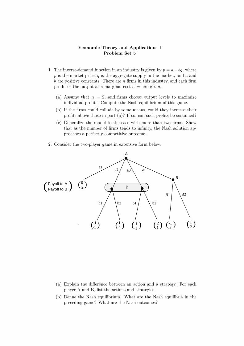
Economic Theory and Applications IProblem Set 5
1. The inverse-demand function in an industry is given by p = a− bq, wherep is the market price, q is the aggregate supply in the market, and a andb are positive constants. There are n firms in this industry, and each firmproduces the output at a marginal cost c, where c < a.
(a) Assume that n = 2, and firms choose output levels to maximizeindividual profits. Compute the Nash equilibrium of this game.
(b) If the firms could collude by some means, could they increase theirprofits above those in part (a)? If so, can such profits be sustained?
(c) Generalize the model to the case with more than two firms. Showthat as the number of firms tends to infinity, the Nash solution ap-proaches a perfectly competitive outcome.
2. Consider the two-player game in extensive form below.
A
B
-1-1
1 0
-1-1
2 1
02
Payoff to APayoff to B( ) ( )
( )( )( ) ( )
a1a2 a3 a4
b1 b1b2 b2
B2B1
B
-1-1
( ) 12( )
(a) Explain the difference between an action and a strategy. For eachplayer A and B, list the actions and strategies.
(b) Define the Nash equilibrium. What are the Nash equilibria in thepreceding game? What are the Nash outcomes?

Birkbeck Economics 86
(c) Define a subgame perfect Nash equilibrium. What are the subgameperfect Nash equilibria in the preceding game? What are the sub-game perfect outcomes?
(d) Do you consider the notion of subgame perfection appealing? Is itadequate in the context of the game above, and if not, why?
3. Consider the following two-player game. Player 1 chooses a row (Top,Middle, or Bottom) and, simultaneously, player 2 chooses a column (Left,Centre, or Right). Each cell in the outcome matrix specifies the payoffsto players 1 and 2 respectively, for each combination of choices made bythem.
Player 2
Left Middle RightTop 7,2 6,5 3,3
Player 1 Middle 3,5 3,3 5,6Bottom 5,6 2,6 4,7
(a) What does the term “dominated strategy” mean in the context ofgames such as this? Are there any dominated strategies in this game?
(b) What is meant by a Nash equilibrium? Identify all the pure-strategyNash equilibria in the above game.
(c) Are there any mixed-strategy Nash equilibria? If so, which strategiesare not used in the equilibrium randomization?
4. Consider the following simultaneous move game.
Player 2
L RT 5,5 0,6
Player 1 B 6,0 1,1
(a) Solve the game without invoking Nash equilibrium.
(b) Nash equilibrium has certain restrictive features. Describe one suchfeature that you do not need to rely upon in order to solve this game.
(c) How would the equilibrium behaviour change if the game is playedtwice?

Birkbeck Economics 87
5. Consider the following extensive form game. The entrant moves first anddecides whether to enter. If he decides to enter, he then decides whether toproduce bathtubs (B) or jacuzzis (J). The incumbent observes the decisionabout entry, but not the decision about product choice. The incumbentfaces the same choice of products (b,j).
(a) Write down the actions and strategies available to each player.
(b) Define Nash equilibrium and subgame perfect equilibrium. For anygame, what is the relationship between the set of Nash equilibria andthe set of subgame perfect equilibria?
(c) Find the subgame perfect equilibria of the game.
(d) Find the Nash equilibria of the game. How does the set of Nash equi-libria of this game differ from the set of subgame perfect equilibriathat you derived in part (c)?
Entrant
Entrant
Incumbent
O
I
B J
b j b j
-3-3
1-1
-1 1
-6-6
02
Payoff to EntrantPayoff to Incumbent( )
( )
( )( )( ) ( )

Economic Theory and Applications IProblem Set 6
1. Consider a second-hand car market with two kinds of cars, type A whichare completely reliable, and type B which break down with probability1/2. There are 20 car owners, 10 with each kind of car, and 19 potentialbuyers. The car owners and buyers value a car at £1000 and £1500,respectively if it works and both owners and buyers value a non-workingcar at zero. Both buyers and owners are assumed to be price takers andrisk-neutral. Finally each seller is aware of the type that her car belongsto, but this information is not available to buyers.
(a) What value do buyers and sellers place on type A and type B cars?
(b) How many cars, and of what quality will be supplied at each price?(Quality is defined as the proportion of cars that are of type A.)
(c) Given that buyers can observe the market price, and have rationalexpectations, what will be the demand for cars at each price?
(d) How many equilibria are there in the market?
2. Suppose the quality of a used car can be indexed by some number q.Buyers are willing to pay (3/2)q for a car of quality q, and sellers arewilling to sell a car of quality q for a price of q.
(a) What is the equilibrium in the market if q is observable?
(b) Now suppose that the quality is known to the seller, but not to thebuyers. The buyers only know that q is distributed uniformly over[0, 1]. What is the equilibrium now?
3. Suppose we introduce equity contracts in the Stiglitz-Weiss model. Showthat now markets clear and there is no longer any rationing of credit.
4. Finally, here is problem concerning alternative models of the credit mar-ket. We will not discuss this in the class, but if you are interested in thesubject, you should think about this.
Construct a model similar to the Stiglitz-Weiss model by assuming thatthe projects are equally risky, but they have different expected payoffs.Suppose, for example, that the probability of success p of a project is arandom variable with a uniform distribution on [0, 1]. Show that in thissetup debt contracts are optimal, and the equilibrium is characterized byoverinvestment rather than underinvestment.

Economic Theory and Applications IProblem Set 7
1. Consider the following principal-agent model. A principal hires an agentto work on a project in return for wage payment w > 0. The agent’sutility function is separable in the effort and wage received: we haveu(w, ei) = v(w) − g(ei), where v(.) is his von-Neumann Morgernsternutility function for money, and g(ei) is the disutility associated with effortlevel ei exerted on the project.
Assume that the agent can choose one of two possible effort levels, e1 ore2, with associated disutility levels g(e1) = 5/3, and g(e2) = 4/3. Thevalue of the project’s output depends on the agent’s chosen effort levelin a probabilistic fashion: If the agent chooses effort level e1, the projectyields output πH = 10 with probability p(H|e1) = 2/3, and πL = 0 withthe residual probability. If the agent chooses effort level e2, the projectyields πH = 10 with probability p(H|e2) = 1/3, and πL = 0 with theresidual probability.
The principal is risk neutral: she aims to maximize the expected valueof the output, net of any wage payments to the agent. The agent isrisk-averse, with v(w) =
√w, and his reservation utility equals 0.
(a) Suppose, first, that the effort level chosen by the agent is observableby the principal. A wage contract then specifies an effort level e∗,and an output-contingent wage schedule {wH , wL}. Here wH is thewage paid if π = πH , and wL the wage if π = πL. Show that if effortis observable, it is optimal for the principal to choose a fixed wagecontract (that is, wH = wL = w∗). Provide brief intuition for thisresult.
(b) If effort is observable, what wage w∗ should the principal offer if shewants to implement e1? What wage implements e2? Which inducedeffort level provides a higher expected return to the principal, net ofwage costs?
(c) Suppose, next, that the agent’s choice of effort level is not observable.In this circumstance, a contract consists of an output- contingentwage schedule {wH , wL}. What wage schedule will implement e1 inthis case. What expected net return does the principal get in thiscase? How does this compare with the value in part (b), where effortwas observable.
(d) If effort is not observable, what contract is best for the principal?Should she implement e1 or e2?
2. A principal hires an agent to work on a project in return for wage w.However, the principal could also “punish” the agent by inflicting a utilityloss of F , where F ∈ [0,∞). The agent’s utility is given by
u(w, ei) =√
w − F − g(ei)

Birkbeck Economics 90
where g(ei) is the disutility associated with effort level ei exerted on theproject. Assume that the agent can choose one of two possible effortlevels, e1 or e2, with associated disutility g(e1) = 1, and g(e2) = 0. Thereare three states of the world, H, M and L, with associated returns 10, 6and 0 respectively. If the agent chooses effort level e1, the project yieldsthe following distribution of returns:
10 (state H) with probability 1/26 (state M) with probability 1/2.
If the agent chooses effort level e2, the distribution of returns is
10 (state H) with probability (1 − ε)/26 (state M) with probability (1 − ε)/20 (state L) with probability ε.
where 0 < ε ≤ 1. The principal is risk neutral and aims to maximize theexpected value of returns net of wage payments. The agent’s reservationutility is 0. A contract specifies a wage schedule {wH , wM , wL}, andpunishment levels {FH , FM , FL}.(a) Suppose, first, that the effort level chosen by the agent is observable
by the principal, and the principal can make the wage contingenton effort. Show that, to implement any level of effort, it is optimalto choose a wage for that effort level which is independent of therealization of return (i.e. wH = wM = wL = w∗), and no punishment(i.e. FH = FM = FL = 0). (A precise statement of the intuitionwould suffice.)
(b) If effort is observable, what wage should the principal offer if shewants to implement e1? What wage implements e2?
(c) Suppose, next, that the agent’s choice of effort level is not observ-able. Show that for any ε such that 0 < ε ≤ 1, effort level e1 can beenforced (i.e. satisfies both the incentive constraint and the partici-pation constraint) by the following wage schedule:
wH = wM = 1wL = 0FH = FM = 0FL = 1−ε
ε
(d) When effort is not observable, what wage schedule implements e2 ?
(e) Show that irrespective of observability of effort it is optimal for theprincipal to implement e2 whenever ε < 1/8.
(f) Prove that when effort is unobservable, there is no wage schedulethat implements the high effort and is cheaper (for the principal)than the wage schedule in part (c). Hint: What parts of the wageschedule in part (c) actually get paid in any equilibrium with higheffort? Compare those with your answer to part (b).

Birkbeck Economics 91
3. Consider the following hidden action model with three possible actionsfor the agent E = {e1, e2, e3}. There are two possible profit outcomesfor the Principal : πH = 10 and πL = 0. The probabilities of πH condi-tional on the three effort levels are f(πH |e1) = 2/3, f(πH |e2) = 1/2, andf(πH |e3) = 1/3. The agent has a separable utility function u(w, ei) =v(w) − g(ei), where v is the von-Neumann Morgernstern utility of wagew, and g(ei) is the disutility of effort. We are told that g(e1) = 5/3,g(e2) = 8/5, and g(e3) = 4/3. Finally, v(w) =
√w and that the man-
ager’s reservation utility is u = 0.
(a) What is the optimal contract when effort is observable?
(b) Show that if effort is not observable, then e2 is not implementable.For what level of g(e2) would e2 be implementable? [Hint: focus onthe utility the manager will get for the two outcomes].
(c) What is the optimal contract when effort is not observable?
4. A principal hires an agent to work on a project at wage w. The agent’sutility function is
U(w, ei) = 100 − 10w
− g(ei),
where g(ei) is the disutility associated with the effort level ei exerted onthe project. The agent can choose one of two possible effort levels, e1 ore2, with associated disutility levels g(e1) = 50, and g(e2) = 0. The agent’schoice of effort affects the project’s output in a probabilistic fashion: ifthe agent chooses effort level e1, an error occurs in the production processwith probability 1/4, and if he chooses e2, an error occurs with probability3/4. The project yields a revenue of 20 if the production process is errorfree, and a revenue 0 otherwise. The principal is risk neutral: she aims tomaximize the expected value of the output, net of any wage payments tothe agent. The agent has a reservation utility of 0.
(a) If the effort level chosen by the agent is observable by the principal, itis optimal for the principal to choose a fixed-wage contract. Explainthe intuition for this result.
(b) If effort is observable, what wage w∗ should the principal offer if shewants to implement e1? What wage implements e2? Which of thesewill the principal implement?
(c) Suppose that the agent’s choice of effort level is not observable. Whatwage schedule will implement e1 in this case? What expected netreturn does the principal get in this case? How does this comparewith the value in part (b), where effort was observable?
(d) If effort is not observable, should the principal implement e1 or e2?

Economic Theory and Applications IProblem Set 8
1. Consider a first-price sealed-bid auction in which the bidders’ valuationsare independently and uniformly distributed on [0, 1]. Show that if thereare n bidders, then the strategy of bidding (n−1)/n times one’s valuationis an equilibrium of this game.
2. (a) Consider an auction with N > 1 symmetric, risk-neutral bidderswhose private valuations vi, i ∈ {1, . . . , N} are independent drawsfrom a given distribution F on the interval [0, V ]. Prove that ina second price auction the Nash Equilibrium in weakly dominantstrategies involves bidders bidding their true values.
(b) Consider the following second-price common-value auction with twobidders. For both bidders, the value of the object being auctioned isV1 +V2 where V1 and V2 are independent random variables. Bidder iknows the realization of Vi, i ∈ {1, 2}. Show that, for any realizationvi of Vi, a bid of 2vi by bidder i, i ∈ {1, 2}, is a Nash Equilibriumin this second-price auction. (Hint: Suppose 2 bids 2v2, and 1 bidsx. Compare a bid of x �= 2v1 to a bid of x = 2v1. Use argumentssimilar to the ones used in the answer to part (a).)
3. If the auctioneer could generate false bids after the bids are received,bidding one’s true value in a second-price auction would no longer be anequilibrium. Discuss.