Embed Size (px)
Citation preview

Auxetic Behaviour of Re-entrant Cellular
Structured Kirigami at The Nanoscale
Jing Luo
B.E. (Beihang University, P.R. China)
Supervised by Prof. Qinghua Qin
February 2017
A thesis submitted for the degree of Master of Philosophy
of The Australian National University
Research School of Engineering
College of Engineering & Computer Science
The Australian National University

To my family
For their endless love and support
Declaration
This thesis contains no material which has been previously accepted for the
award of any other degree or diploma in any university, institute or college. To
the best of the author’s knowledge, it contains no material previously published
or written by another person, except where due reference is made in the text.
Jing Luo
Research School of Engineering
College of Engineering & Computer Science
The Australian National University
28 February 2017
Signature_____________________
© Jing Luo 2017
All Rights Reserved

iv
Acknowledgments
First and foremost, I would like to show endless and sincere gratitude to my
primary supervisor and also the chair of my supervisory panel, Prof. Qinghua
Qin, without whom my research journey would not have been possible. He has
always been supportive and taught me so much about how to do high-quality
research. Besides, I also would like to express my thanks and appreciation to my
associate supervisor, Dr. Yi Xiao, for being so enthusiastic, supportive and
helpful over my past years at the Australian National University (ANU). I will
surely benefit from this unique training and experience throughout my whole
life.
I am also in debt to Prof. Kun Cai, a visiting research fellow of my
research group, for his advice, guidance and kindness throughout my research
work and thesis manuscript writing. In addition, I am grateful to Jing Wan, an
outstanding student of Prof. Cai, for his encouragements and advices on MD
simulation scripts programming, too.
My sincere thanks also go to our group members for their helpful
suggestions and sincere friendships throughout my research and daily life at
Research Group of Engineering Mechanics, ANU. They are Prof. Hui Wang,
Prof. Hongzhi Cui, Mr. Cheuk-Yu Lee, Mr. Haiyang Zhou, Mr. Song Chen, Ms.
Shuang Zhang, Mr. Bobin Xing, Mr. Shaohua Yan, Ms. Yiru Ling and Ms. Ting
Wang. For all of their help, interesting and valuable hints and comments.
I am also indebted to the people who accompany me at Canberra, Mr.
Tong Zhang, Dr. Xin Yu, Mr. Zhixun Li, Mr. Yan Zhang and Xiaosong Li, who
are my lifetime friends. We have been through both difficulties and
achievements all the way through. There are many great memories that we will
cherish for a long time, such as a journey to the Batemans Bay and ANU Kioloa
Coastal Campus. I sincerely wish all of you a successful future and wonderful
life.

v
Last but not least, especially, I would like to give my special thanks to my
family, my parents and my elder sister, for encouraging me and convincing me
to believe myself and for always trusting me even sometimes I particularly do
not. I promise I will spend my lifetime to reciprocate your endless love and
support.
vi
Abstract
Some typical two-dimensional (2D) materials are active elements used in nano-
electro-mechanical systems (NEMS) design, owing to their excellent in-plane
physical properties on mechanical, electrical and thermal aspects. Considering a
component with a negative Poisson’s ratio used in NEMS, the adoption of
kirigamis made of periodic re-entrant honeycomb structures at the nanoscale
would be a feasible method. The focus of this thesis work is to investigate the
specific auxetic behaviour of this kind of structures from typical tailored 2D
materials. By employing the numerical simulation method: molecular dynamics
simulation, the auxetic behaviour of re-entrant cellular structured kirigami is
discussed thoroughly and concretely.
Three main effects of a re-entrant cellular structured kirigami are
systematically simulated, and then analysed and discussed here. They are size
effect, surface effect and matrix effect of 2D materials. The study begins with a
demonstration that a kirigami with specific auxetic property obtained by
adjusting the sizes of its honeycombs. Making use of molecular dynamics
experiments, the size effect on auxetic behaviour of the kirigami is discussed.
The results show that, in some cases, the auxetic difference between the
microscopic structured kirigami and macroscopic structure kirigami is
negligible, which means the results from macro-kirigami could be used to
predict the auxetic behaviour of nano-kirigami. Surface effect of kirigami is also
illustrated from two aspects. The one is to identify the difference of mechanical
responses between pure kirigami and hydrogenated kirigami at some geometry
and loading condition. And another is from the difference of mechanical
responses between microstructure kirigami and continuum kirigami under the
same loading condition and geometric configuration. Graphene is selected as the
major 2D material in the study. As kirigami tailored from various 2D materials
would exhibit different mechanical behaviour, graphene, single-layer hexagonal
boron nitride (h-BN) and single-layer molybdenum disulphide (MoS2) are

vii
selected as representative 2D materials to investigate the influence of this effect,
without loss of generality.

viii
ContentsDeclaration ............................................................................................................................................................ iii
Acknowledgments ................................................................................................................................................. iv
Abstract ................................................................................................................................................................. vi
Contents ............................................................................................................................................................... viii
List of Figures ........................................................................................................................................................ x
List of Tables ....................................................................................................................................................... xiii
List of Abbreviations .......................................................................................................................................... xiv
Chapter 1 Introduction ................................................................................................................................... 1
1.1 BACKGROUND AND MOTIVATION ............................................................................................................... 1 1.2 OBJECTIVE ................................................................................................................................................. 5 1.3 OUTLINE .................................................................................................................................................... 6
Chapter 2 Literature Review ......................................................................................................................... 7
2.1 PREVIOUS WORK ........................................................................................................................................ 7 2.2 2D MATERIALS ........................................................................................................................................... 8
2.2.1 Graphene ......................................................................................................................................... 8 2.2.2 Hexagonal boron nitride ................................................................................................................. 9 2.2.3 Molybdenum disulphide ................................................................................................................. 10
2.3 AUXETIC MATERIALS ............................................................................................................................... 11 2.3.1 Mechanism of auxetic materials .................................................................................................... 11 2.3.2 Natural auxetic materials .............................................................................................................. 13 2.3.3 Artificial auxetic materials ............................................................................................................ 17 2.3.4 Properties of auxetic materials ...................................................................................................... 20 2.3.5 Applications of auxetic materials .................................................................................................. 21
2.4 SUMMARY ................................................................................................................................................ 23
Chapter 3 Research Methodology ................................................................................................................ 24
3.1 MD SIMULATION...................................................................................................................................... 24 3.1.1 Modelling the N-atom physical system .......................................................................................... 25 3.1.2 Potentials ....................................................................................................................................... 26 3.1.3 Time integration algorithm ............................................................................................................ 28 3.1.4 Ensembles ...................................................................................................................................... 29 3.1.5 Energy minimization ...................................................................................................................... 30 3.1.6 Heating baths ................................................................................................................................. 30 3.1.7 Periodic boundary condition ......................................................................................................... 31 3.1.8 MD software package .................................................................................................................... 32
3.2 STRAIN CALCULATION IN 2D MATERIAL KIRIGAMI .................................................................................. 33
ix
3.2.1 Deformation control method.......................................................................................................... 33 3.2.2 Stress method ................................................................................................................................. 34
3.3 DENSITY FUNCTIONAL THEORY ................................................................................................................ 35 3.4 THEORETICAL ANALYSIS OF RE-ENTRANT CELLULAR STRUCTURE KIRIGAMI ........................................... 36 3.5 SUMMARY ................................................................................................................................................ 38
Chapter 4 Size and surface effects of graphene kirigami .......................................................................... 39
4.1 MODEL DESCRIPTIONS ............................................................................................................................. 39 4.1.1 Geometric model of kirigami ......................................................................................................... 39 4.1.2 Methods for numerical experiments .............................................................................................. 41 4.1.3 Schemes for size effect analysis ..................................................................................................... 43
4.2 NUMERICAL RESULTS AND DISCUSSIONS .................................................................................................. 45 4.2.1 Results on included angle between vertical and oblique bar varying ........................................... 45 4.2.2 Results on the width of oblique bar ............................................................................................... 46 4.2.3 Results on different width of vertical bar ....................................................................................... 47 4.2.4 Results on different length of vertical bar ..................................................................................... 48 4.2.5 Results on different length of oblique bar ...................................................................................... 49
4.3 SUMMARY ................................................................................................................................................ 53
Chapter 5 Effect of different matrix 2D materials ...................................................................................... 55
5.1 MODEL DESCRIPTIONS ............................................................................................................................. 55 5.1.1 Geometric model of kirigami ......................................................................................................... 56 5.1.2 Methods for numerical experiments .............................................................................................. 56
5.2 NUMERICAL RESULTS AND DISCUSSIONS .................................................................................................. 57 5.2.1 Results on different angle between vertical and oblique bar ......................................................... 57 5.2.2 Results on different width of oblique bar ....................................................................................... 59 5.2.3 Results on different width of vertical bar ....................................................................................... 61
5.3 SUMMARY ................................................................................................................................................ 63
Chapter 6 Conclusions and Future Works .................................................................................................. 65
6.1 CONCLUSIONS .......................................................................................................................................... 65 6.2 LIMITATIONS............................................................................................................................................ 66 6.3 FUTURE WORKS ....................................................................................................................................... 67
Bibliography ........................................................................................................................................................ 68
Publications .......................................................................................................................................................... 79
Appendix A .......................................................................................................................................................... 81
Appendix B ........................................................................................................................................................... 84
Appendix C .......................................................................................................................................................... 92
Appendix D .......................................................................................................................................................... 98
x
List of Figures
Figure 1-1: Schematic diagram of different Poisson’s ratio material (a) Positive
ν (b) Negative ν. ............................................................................................. 2
Figure 1-2: Auxetic materials (a) Natural (b) Artificial. ....................................... 3
Figure 1-3: Schematic diagram of tailoring 2D material to re-entrant cellular
structures at the nanoscale. ............................................................................. 4
Figure 2-1: Schematic diagram of graphene53. ..................................................... 9
Figure 2-2: Schematic diagram of h-BN53. ......................................................... 10
Figure 2-3: Schematic diagram of MoS253. ......................................................... 10
Figure 2-4: Auxetic materials exist from molecular level to macroscopic level64.
...................................................................................................................... 12
Figure 2-5: Deformation mechanism of typical auxetic material. The blue dash
lines represent the initial structure of this material. ..................................... 13
Figure 2-6: Cristobalite crystal66 ......................................................................... 13
Figure 2-7: Schematic diagram of cristobalite crystal. (a) Crystal structure of α-
cristobalite (b) The variation in Poisson’s ratio, maximum auxetic behaviour
in the (1 0 0) and (0 1 0) planes (YZ, XZ) at 45° to the major axes67. .......... 14
Figure 2-8: Schematic diagram of zeolite crystal72. ............................................ 15
Figure 2-9: Schematic diagram of zeolite crystal. (a) Crystal structure of zeolite
(b) The value of Poisson’s ratio obtained from different force-field-based
molecular simulations72. ............................................................................... 15
Figure 2-10: The structure of B.C.C. solid metal74. ............................................ 16
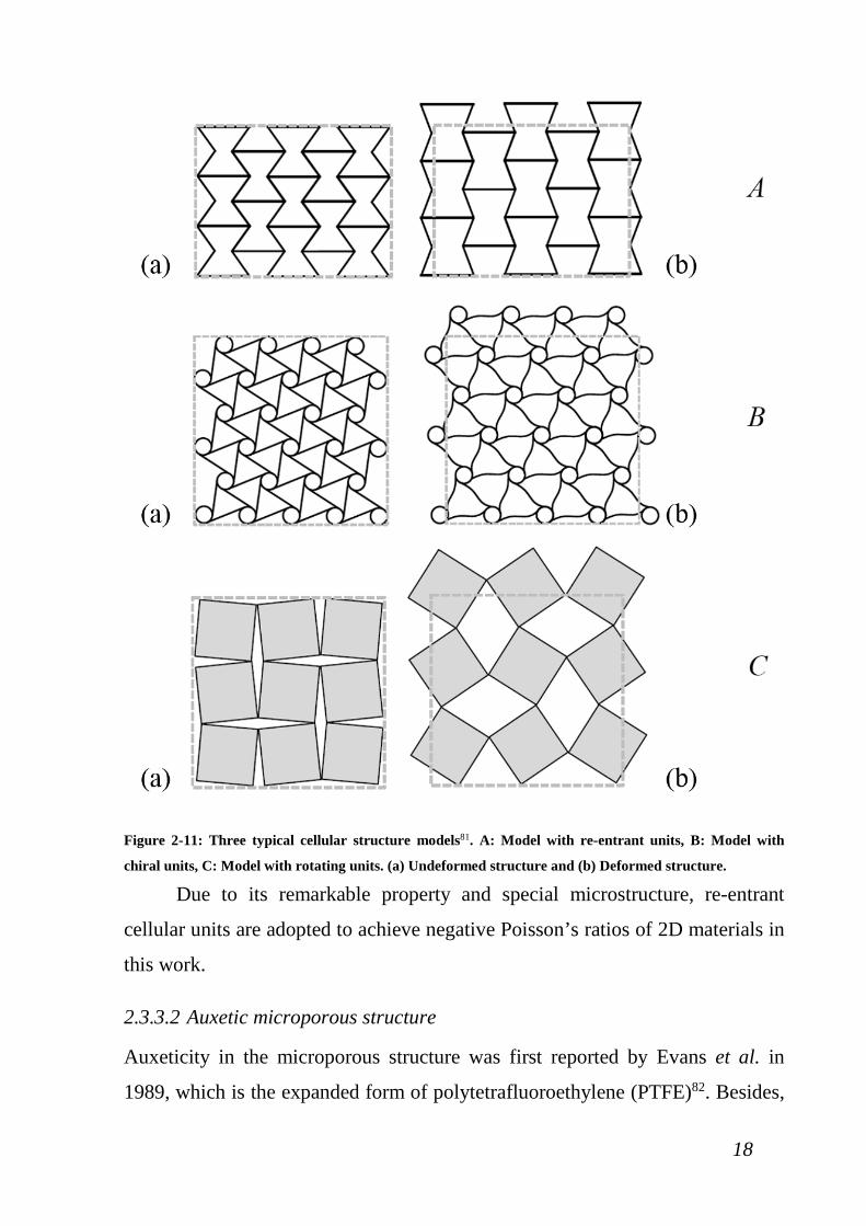
Figure 2-11: Three typical cellular structure models81. A: Model with re-entrant
units, B: Model with chiral units, C: Model with rotating units. (a)
Undeformed structure and (b) Deformed structure. ..................................... 18
Figure 2-12: (a) Microstructure details of PTFE obtained by SEM82, (b)
undeformed and deformed structure of PTFE81. .......................................... 19
Figure 2-13: A periodic fibre reinforced composite with star-shaped
encapsulated inclusions86. ............................................................................ 20

xi
Figure 2-14: Indentation test for (a) non-auxetic and (b) auxetic materials64. ... 21
Figure 2-15: Schematic diagram of artificial blood vessels89. (a) Non-auxetic
materials (b) Auxetic materials. ................................................................... 22
Figure 3-1: A schematic diagram of 3D PBC simulation box113. ....................... 32
Figure 3-2: A flow chart of MD simulation script programming. ...................... 33
Figure 3-3: A part of re-entrant cellular structured kirigami. The right half part
of (a) is a quarter of the unit cell. The grey area represents the domain
whose mechanical property is determined by the oblique bars and the
vertical bars. The vertical bars determine the mechanical property of the
yellow area. (b) The homogenised model of the right half part of (a). E1 and
E2 (<E1) are the in-plane equivalent moduli of the yellow and grey areas,
respectively. (c) The final deformation. ....................................................... 36
Figure 3-4: Simplified homogenized zone. ......................................................... 37
Figure 4-1: Schematic diagram of graphene kirigami with detailed geometric
parameters121. (a) The atomic system with periodic microstructure in the
solid yellow frame. (b) The geometry of local microstructure (in the solid
yellow frame in (a)) with detailed geometric parameters of the kirigami. The
microstructure has one more vertical rod than the unit cell. ........................ 39
Figure 4-2: The finite element model of the continuum kirigami and the local
finite element (FE) mesh in the solid black frame shown right121. .............. 40
Figure 4-3: Schematic diagram of different surface energy model. ................... 42
Figure 4-4: Configurations of the local microstructure of GK with different
geometric parameters in five schemes121. Here N(w) is denoted as the
number of the basic honeycomb atoms along the direction of variable w,
e.g., N(w)=3 in Figure 4-1(b). (a) Scheme 1, θ changes; (b) N(wθ) changes;
(c) N(w) changes; (d) N(lG) changes; (e) N(lθ) changes. .............................. 44
Figure 4-5: Comparison of configurations before and after deformation with
respective to different lengths of oblique bar. In each inserted figure, the
mid microstructure is labelled with a solid lime frame. In each case, the
configuration of the structure is formed with three layers of microstructures.
xii
The upper figure in each case is the initial configuration after relaxation, the
lower figure in each case is the final stable configuration after loading and
relaxation. ..................................................................................................... 51
Figure 4-6: Different contour plot of electron density nearby the neighbour ends
of vertical bars in the initial configuration of the pure carbon GK with (a)
N(lθ)=24 (see the upper layer of Figure 4-5(b)) and (b) N(lθ)>36 obtained by
the calculation using first principles 126. ....................................................... 52
Figure 5-1: Cell model of re-entrant cellular structured kirigami made of
different 2D materials, Graphene Kirigami, h-BN Kirigami and MoS2
Kirigami. For the convenience of observation, same length scale is not
adopted here.................................................................................................. 55
Figure 5-2: Configurations of local microstructure of the kirigami with different
geometric parameters in three schemes. Here N(w) is denoted as the number
of the honeycomb atoms along the direction of variable w, e.g., N(w) = 3 in
Figure 4-1(b). (a) Scheme 1, θ changes; (b) N(wθ) changes; (c) N(w)
changes. ........................................................................................................ 56
Figure 5-3: Results on included angle between vertical and oblique bar varying.
(a) Rp (b) Rm .................................................................................................. 58
Figure 5-4: Results on width of oblique bar varying. (a) Rp (b) Rm .................... 60
Figure 5-5: Results on width of vertical bar varying. (a) Rp (b) Rm .................... 62
xiii
List of Tables
Table 4-1: Comparisons of Poisson’s ratio and the modulus ratio for the three
models in Scheme 1. ..................................................................................... 45
Table 4-2: Comparisons of Poisson’s ratio and the modulus ratio for the three
models in Scheme 2. ..................................................................................... 46
Table 4-3: Comparisons of Poisson’s ratio and the modulus ratio for the three
models in Scheme 3. ..................................................................................... 47
Table 4-4: Comparisons of Poisson’s ratio and the modulus ratio for the three
models in Scheme 4. ..................................................................................... 49
Table 4-5: Comparisons of Poisson’s ratio and the modulus ratio for the three
models in Scheme 5. ..................................................................................... 50
Table 5-1: Comparisons of Poisson’s ratio and the modulus ratio for the three
models in Scheme 1. ..................................................................................... 58
Table 5-2: Comparisons of Poisson’s ratio and the modulus ratio for the three
models in Scheme 2. ..................................................................................... 60
Table 5-3: Comparisons of Poisson’s ratio and the modulus ratio for the three
models in Scheme 3. ..................................................................................... 62
xiv
List of Abbreviations 2D …… Two-Dimensional
AIREBO …… Adaptive Intermolecular Reactive Empirical Bond Order
AMBER …… Assisted Model Building with Energy Refinement
B.C.C. …… Body Centred Cubic
BK …… Hexagonal boron nitride Kirigami
BP …… Black Phosphorus
CG …… Conjugate Gradient
CHARMM …… Chemistry at HArvard Macromolecular Mechanics
CK …… Continuum Kirigami
DFT …… Density Functional Theory
F.C.C …… Face Centred Cubic
FEM …… Finite Element Method
FET …… Field-Effect Transistor
fs …… Femtosecond
GK …… Graphene Kirigami
GROMACS …… GROningen MAchine for Chemical Simulations
h-BN …… hexagonal Boron Nitride
LAMMPS …… Large-scale Atomic/Molecular Massively Parallel Simulator
MD …… Molecular Dynamics
MEMS …… Micro-Electro-Mechanical Systems
MK …… Molybdenum disulphide Kirigami
MoS2 …… Molybdenum Disulphide
NAMD …… NAnoscale Molecular Dynamics
NEMS …… Nano-Electro-Mechanical Systems
nm …… Nanometre
NPT …… Isothermal–Isobaric Ensemble
NVE …… Microcanonical Ensemble
NVT …… Canonical Ensemble
PBC …… Periodic Boundary Conditions
ps …… Picosecond

xv
PTFE …… Polytetrafluoroethylene
SADS …… Sil AD Spezial
SEM …… Scanning Electron Microscope
SW …… Stillinger-Weber
UHMWP …… Ultra-High-Molecular-Weight Polyethylene
ν …… Poisson’s ratio

1
Chapter 1 Introduction
1.1 BACKGROUND AND MOTIVATION
Nowadays, auxetic materials and two-dimensional (2D) materials have been two
of the most active research fields for many years in material science1. Recently,
the two formerly independent fields have started to intersect in quite new and
interesting ways. Consequently, it becomes possible to some extent to take full
advantages of the auxetic property in 2D materials by optimizing their
microstructures, and particularly to apply the structure in the rapidly developed
micro-electromechanical systems (MEMS) and nano-electromechanical systems
(NEMS)2.
First of all, the 2D materials are a class of nanomaterials defined by their
property of being merely one or two atoms thick. These categories of
nanomaterials are thinned to their physical limits, and thus exhibit novel
properties different from their bulk counterpart3. These 2D materials mainly
include graphene, hexagonal boron nitride (h-BN) and single-layer Molybdenum
Disulphide (MoS2), etc4. Since the (re)discovery of 2D material, the single-layer
graphene, in 2004 by Novoselov and Geim5, they have gained extensive
attention in a variety of fields of nano-engineering6–8, due to their remarkable
mechanical, electrical, and thermal properties9. All of these properties make 2D
materials a good candidate in the application to micro-electromechanical
systems (MEMS) and nano-electromechanical systems (NEMS)2. Some research
efforts have been devoted to discovering the potential applications of the 2D
materials in the fabrication of nano-devices. As a result, they could, as raw
materials, be made into gigahertz oscillators10, nano-pumps11, nano-bearings12,
nano strain-sensors13–15, and many other nano-devices16–20.
Moreover, the auxetic materials are those engineering structures that have a
negative Poisson’s ratio21. Here, the Poisson’s ratio, ν, could be expressed as,

2
.trans
axial
εν
ε= − (1.1)
where εtrans represents transverse strain and εaxial represents axial strain. It
characterizes the negative ratio of the transverse normal strain to the axial
normal strain for a sample of material subjected to an axial loading22,23. When
stretched, these specific materials become thicker in the direction perpendicular
to the applied force. For illustration, Figure 1-1 intuitively presents the behavior
of different Poisson’s ratio materials under tensile test.
Figure 1-1: Schematic diagram of different Poisson’s ratio material (a) Positive ν (b) Negative ν.
As aforementioned, since the auxetic materials are able to exhibit novel
behaviour under deformation, they are of great interest in the field of material
science. Recently, the design and synthesis of such auxetic materials at the
nanoscale level is a research hotspot. For most traditional materials, the
Poisson’s ratio is typically a positive number and has a value around 0.3 in a
large number of engineering materials, such as steels. While, a lot of natural
materials have been reported to be auxetic24,25, they exist extensively in actual
engineering. In Figure 1-2, the two major types of auxetic materials in the actual
engineering is shown, with the first one the natural and another fabricated from
industry, 69% of the cubic metal crystals and some face-centred cubic(F.C.C)
rare gas solids for instance behaved auxetic when they were stretched along a
non-axial direction26,27. As for artificial materials, there are also many auxetic
materials developed and invented, which is very popular in practical engineering
field. And they could be found in many structures, such as honeycomb28,
3
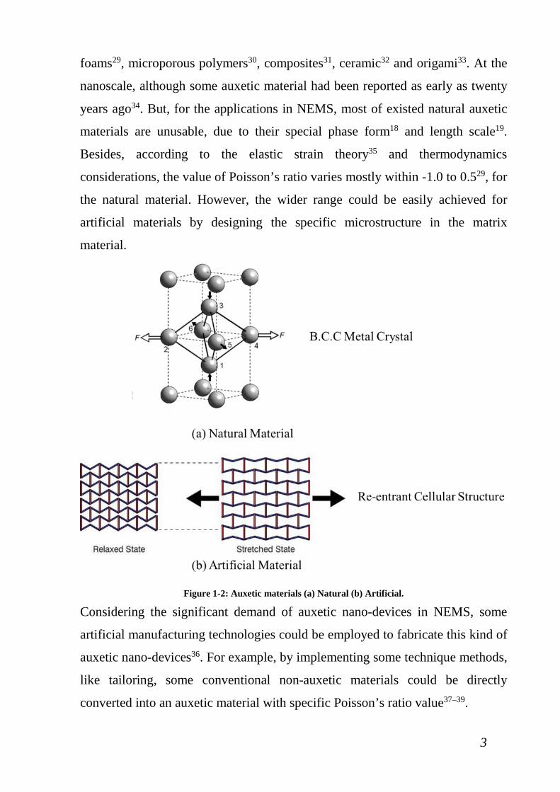
foams29, microporous polymers30, composites31, ceramic32 and origami33. At the
nanoscale, although some auxetic material had been reported as early as twenty
years ago34. But, for the applications in NEMS, most of existed natural auxetic
materials are unusable, due to their special phase form18 and length scale19.
Besides, according to the elastic strain theory35 and thermodynamics
considerations, the value of Poisson’s ratio varies mostly within -1.0 to 0.529, for
the natural material. However, the wider range could be easily achieved for
artificial materials by designing the specific microstructure in the matrix
material.
Figure 1-2: Auxetic materials (a) Natural (b) Artificial.
Considering the significant demand of auxetic nano-devices in NEMS, some
artificial manufacturing technologies could be employed to fabricate this kind of
auxetic nano-devices36. For example, by implementing some technique methods,
like tailoring, some conventional non-auxetic materials could be directly
converted into an auxetic material with specific Poisson’s ratio value37–39.
4
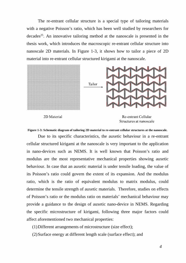
The re-entrant cellular structure is a special type of tailoring materials
with a negative Poisson’s ratio, which has been well studied by researchers for
decades25. An innovative tailoring method at the nanoscale is presented in the
thesis work, which introduces the macroscopic re-entrant cellular structure into
nanoscale 2D materials. In Figure 1-3, it shows how to tailor a piece of 2D
material into re-entrant cellular structured kirigami at the nanoscale.
Figure 1-3: Schematic diagram of tailoring 2D material to re-entrant cellular structures at the nanoscale.
Due to its specific characteristics, the auxetic behaviour in a re-entrant
cellular structured kirigami at the nanoscale is very important to the application
in nano-devices such as NEMS. It is well known that Poisson’s ratio and
modulus are the most representative mechanical properties showing auxetic
behaviour. In case that an auxetic material is under tensile loading, the value of
its Poisson’s ratio could govern the extent of its expansion. And the modulus
ratio, which is the ratio of equivalent modulus to matrix modulus, could
determine the tensile strength of auxetic materials. Therefore, studies on effects
of Poisson’s ratio or the modulus ratio on materials’ mechanical behaviour may
provide a guidance to the design of auxetic nano-device in NEMS. Regarding
the specific microstructure of kirigami, following three major factors could
affect aforementioned two mechanical properties:
(1) Different arrangements of microstructure (size effect);
(2) Surface energy at different length scale (surface effect); and
5
(3) Matrix effect of 2D materials.
However, at nano length scale, the classical continuum mechanics theory is
no longer suitable for investigating those effects on the mechanical properties of
auxetic kirigami. In addition, due to the large consumptions and limitations of
real experiments, there are still many essential issues remain puzzled. Here,
molecular dynamics (MD) simulation, which is the most effective method for
the study of mechanical behaviour at the nanoscale, is employed to study the
influence of the factors discussed above.
The analysis of mechanical properties in re-entrant cellular structured
kirigami in this study is expected to provide some constructive suggestions to
the potential applications to nano-devices.
1.2 OBJECTIVE
As discussed in Section 1.1, the innovative idea of this research work is to
introduce the macroscopic re-entrant cellular structure into nanoscale structures
by tailoring the single-layer 2D materials. As a result, the major objective of this
work is to explore how the auxetic behaviour of tailored 2D material kirigami is
affected by its geometric arrangements, surface energy and matrix 2D materials
using MD simulation. Some theoretical analyses are also described to verify and
illustrate the influences mentioned above.
There are three major effects covered in this thesis. According to the
geometric arrangement of a single unit re-entrant cellular structure in the
tailored kirigami, size effects of the five main variables showing in the unit cell
(Figure 4-1(b)) are investigated. Next, in order to show the effect of surface
energy on the mechanical property of the Kirigami, the hydrogenation schemes
and continuum schemes are employed. At the end, to figure out the effect of
manufacturing 2D raw materials, further discussions on this issue are given.
Besides, some shortcomings and future work in the field of this thesis project are
presented.
6
1.3 OUTLINE
This thesis consists of six chapters and the rest of dissertation is organized as
follows: Firstly, Chapter 2 begins with a brief review on the existing work
related to this research. Then, a comprehensive summary of 2D materials,
auxetic materials and their unique properties, as well as their applications are
described. Chapter 3 describes the research methodology used in this work,
which includes MD simulations, density functional theory and theoretical
mechanics analysis of composite materials. In particular, details of these
methods are described in this chapter for the reference and notation of late
chapters. In Chapter 4, the results of MD simulations on the graphene kirigami
are reported. Detailed discussions regarding the size effect and surface effect are
presented in this chapter. A comprehensive study on the effect of kirigami
tailored from different matrix 2D materials is presented in Chapter 5. In the end,
chapter 6 presents a summary of the outcomes of the thesis work is provided.
Furthermore, some future work in this field and limitations of this work are
demonstrated.

7
Chapter 2 Literature Review
2.1 PREVIOUS WORK
Materials at the nanoscale with a negative Poisson’s ratio, i.e., auxetics, are
becoming increasingly popular as a result of their remarkable properties. In
recent years, significant advances have been made in the design of nano-devices
utilising the specific characteristics of this category of materials. These advances
are either numerical or experimental.
In the respect of real experiment, the findings of artificial materials at the
nanoscale and with a negative Poisson’s ratio could be dated back to 1999, Xu et
al. used soft lithography to fabricate the auxetic materials with re-entrant cellular
microstructures40. Later, Hall et al. found that the in-plane Poisson’s ratio of
carbon nanotube sheets could be tuned from positive to negative by mixing
single-walled and multi-walled nanotubes41. In 2010, Bertoldi et al. discovered
that the pattern transformations in additional curing silicone rubber Sil AD
spezial (SADS) could lead to unidirectional negative Poisson’s ratio behaviour
only under compression test42. By employing the contemporary advanced
fabrication techniques, some of the materials could be made auxetic. However,
all of the aforementioned real experiments are at micrometre scale, which is
1000 times longer than nanoscale. To bypass this hurdle, a kind of kirigami at
the nanoscale is introduced here. Here, the kirigami is a variation of origami that
includes cutting of a paper43. It originated from Japan, where “kiru” means “cut”
and “kami” means paper. Blees et al. used patterning methods to manipulate
graphene kirigami in building robust nanoscale structures with tunable
mechanical behaviour43.
In numerical respect, Grima et al. presented some MD simulations that
showed how the conformation of graphene could be modified through the
introduction of defects so as to make it amenable to exhibit auxetic38. Jiang et al.
discovered that edge induced warping in monolayer graphene and single-layer
black phosphorus would make them show auxetic behaviour24,44. In contrast to
8
the work of Blees’ experiments, researchers including Qi45, Hanakata46, Gao47
and Wei48, utilised MD simulations to investigate the properties of graphene
kirigami. It can be concluded that MD simulation is a very powerful tool in the
study on mechanical behaviour of nanoscale kirigami.
In this work, the macroscopic re-entrant cellular structures will be
introduced at the nanoscale by tailoring the single-layer 2D material. By
employing MD approach, the auxetic behaviour of this specific micro-structured
materials at the nanoscale is investigated.
2.2 2D MATERIALS
Many layered materials contain strong in-plane covalent bonds and weak
coupling interactions between layers. Such layered structures could be exfoliated
into individual atomic layers. Those layers with one dimension strictly limited to
one single-layer are named 2D material49. The background of 2D materials can
be traced back to 2004 attributed to graphene50. Since then, extensive research
efforts are dedicated to making significant progress in basic science and
applications of this category of material51. The Kirigami made of 2D materials
including graphene, single-layer hexagonal boron nitride and single-layer
molybdenum disulphide is our focus in this thesis.
2.2.1 Graphene
Among the family of 2D materials, graphene is most popular around the world.
Due to generating exfoliation manufacturing method of graphene, Geim and
Novoselov were awarded jointly the Nobel Prize in Physics in 201052. As a
popular 2D material, the physical properties of graphene have been extensively
investigated.
Graphene is a single atomic plane of graphite, which consists of a single-
layer of carbon atoms arranged in a 2D honeycomb lattice. Despite being a 2D
material that is only one plane of atoms thick, monolayer graphene exhibits
9
some desirable mechanical properties, such as large surface area, high Young’s
modulus and excellent thermal conductivity.
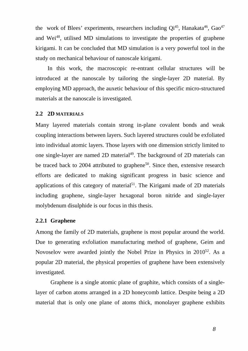
Figure 2-1: Schematic diagram of graphene53.
Graphene has attracted intensive attentions not only for its unusual
physical properties aforementioned, but also for its potential as a basic building
block for a wealth of device applications. Some examples of the structural and
geometric diversity that can be achieved by using kirigami for graphene have
already been demonstrated experimentally43.
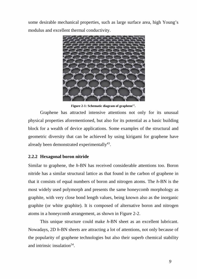
2.2.2 Hexagonal boron nitride
Similar to graphene, the h-BN has received considerable attentions too. Boron
nitride has a similar structural lattice as that found in the carbon of graphene in
that it consists of equal numbers of boron and nitrogen atoms. The h-BN is the
most widely used polymorph and presents the same honeycomb morphology as
graphite, with very close bond length values, being known also as the inorganic
graphite (or white graphite). It is composed of alternative boron and nitrogen
atoms in a honeycomb arrangement, as shown in Figure 2-2.
This unique structure could make h-BN sheet as an excellent lubricant.
Nowadays, 2D h-BN sheets are attracting a lot of attentions, not only because of
the popularity of graphene technologies but also their superb chemical stability
and intrinsic insulation54.
10
Figure 2-2: Schematic diagram of h-BN53.
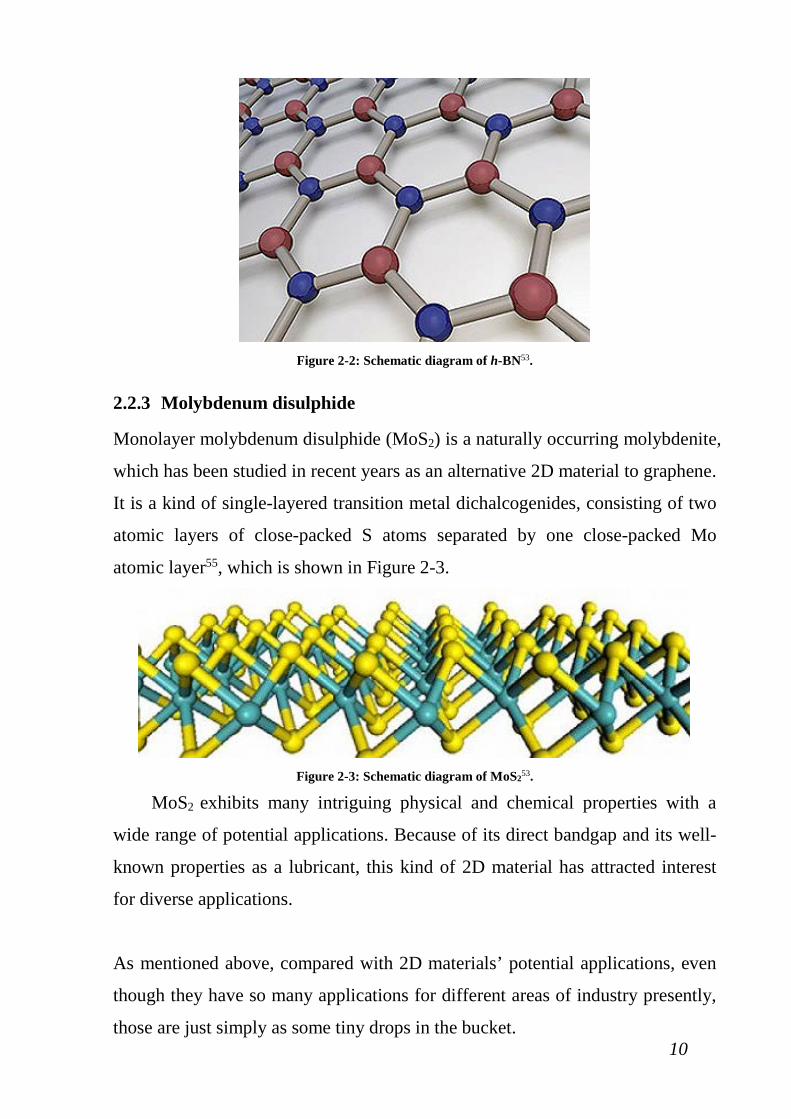
2.2.3 Molybdenum disulphide
Monolayer molybdenum disulphide (MoS2) is a naturally occurring molybdenite,
which has been studied in recent years as an alternative 2D material to graphene.
It is a kind of single-layered transition metal dichalcogenides, consisting of two
atomic layers of close-packed S atoms separated by one close-packed Mo
atomic layer55, which is shown in Figure 2-3.
Figure 2-3: Schematic diagram of MoS253.
MoS2 exhibits many intriguing physical and chemical properties with a
wide range of potential applications. Because of its direct bandgap and its well-
known properties as a lubricant, this kind of 2D material has attracted interest
for diverse applications.
As mentioned above, compared with 2D materials’ potential applications, even
though they have so many applications for different areas of industry presently,
those are just simply as some tiny drops in the bucket.
11
2.3 AUXETIC MATERIALS
Auxetic materials are a kind of materials that have a unique characteristics
where they would expand laterally when stretched, or shrink laterally when they
are compressed. Following subsections would discuss the mechanism of auxetic
materials and some typical auxetic materials.
2.3.1 Mechanism of auxetic materials
When a material is uniaxially loaded in tension, it extends in the direction of the
applied load, which extension is accompanied by a lateral deformation. The
lateral deformations are quantified by a property known as the Poisson’s ratio
which is defined in mathematical terms as the negative ratio of the transverse
over longitudinal strains, as mentioned in equation(1.1). In particular, for
stretching in the x-direction, the Poisson’s ratio in the xy plane of the material is
defined by equation(1.1):
.yxy
x
εν
ε= (2.1)
Even though, the value of Poisson’s ratio was always assumed to be
positive since most everyday materials get thinner when stretched. Today, it has
been shown through numerous studies that negative Poisson’s Ratio materials
exist, meaning that referring to Figure 1-2(b), for the xy plane, a uniaxial load in
the x-direction results in an extension in the y-direction. The existence of these
materials confirms what had been predicted by theory for a long time, the
classical theory of elasticity23 states that the Poisson’s ratio for three-
dimensional isotropic materials may range between -1≤ν≤0.529, while for two-
dimensional isotropic materials, it may range between -1≤ν≤156, with no upper
or lower bounds for anisotropic materials. Some terms have been produced to
describe these counterintuitive materials, such as auxetic21, dilational57, ‘anti-
rubber’58 and ‘self-expanding’59, however, today, the word auxetic is commonly
used in the material science area.
12
Up to now, a lot of auxetic materials have been discovered, the negative
Poisson’s behaviour could be revealed by the intrinsic of the micro or
nanostructure of the materials and the way that this geometric arrangement
deforms on the tensile test. In fact, there are various geometric arrangements
based deformation mechanisms presented to illustrate the auxetic behaviour in
different natural occurring auxetic materials, including cubic metal crystals26, α-
cristobalite60 and liquid crystalline polymers61 and in different artificial auxetic
materials, such as micro/nanostructured polymers62 and foams63. Auxetic
behaviour is scale independent and the similar combination of geometry and
deformation mechanism can operate at any length scale level. Figure 2-4 shows
various discovered auxetic materials at different length scale level.
Figure 2-4: Auxetic materials exist from molecular level to macroscopic level64.
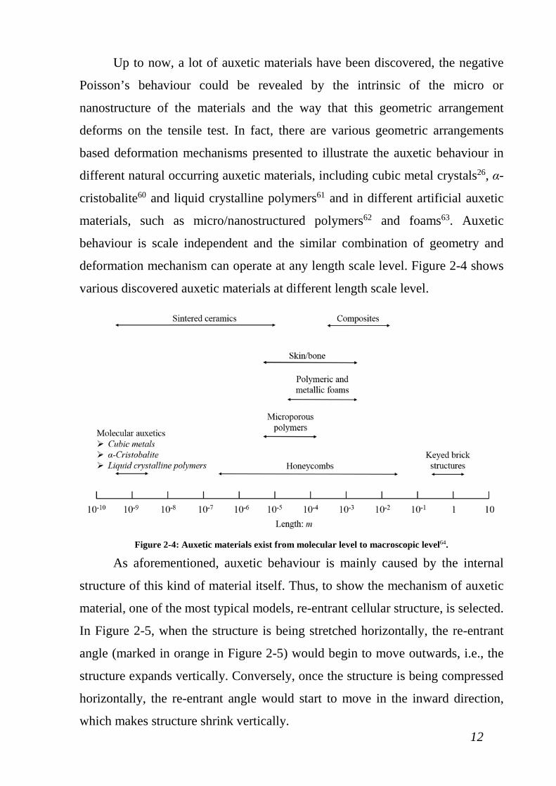
As aforementioned, auxetic behaviour is mainly caused by the internal
structure of this kind of material itself. Thus, to show the mechanism of auxetic
material, one of the most typical models, re-entrant cellular structure, is selected.
In Figure 2-5, when the structure is being stretched horizontally, the re-entrant
angle (marked in orange in Figure 2-5) would begin to move outwards, i.e., the
structure expands vertically. Conversely, once the structure is being compressed
horizontally, the re-entrant angle would start to move in the inward direction,
which makes structure shrink vertically.
13
Figure 2-5: Deformation mechanism of typical auxetic material. The blue dash lines represent the initial
structure of this material.
It should be mentioned that many natural materials have been found to be
auxetic in the practical engineering65. In the category of artificial or man-made
materials, auxetic materials are also popular.
2.3.2 Natural auxetic materials
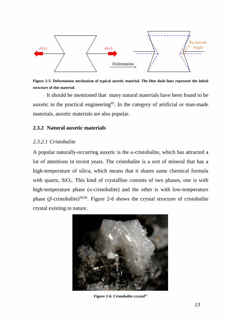
2.3.2.1 Cristobalite
A popular naturally-occurring auxetic is the α-cristobalite, which has attracted a
lot of attentions in recent years. The cristobalite is a sort of mineral that has a
high-temperature of silica, which means that it shares same chemical formula
with quartz, SiO2. This kind of crystalline consists of two phases, one is with
high-temperature phase (α-cristobalite) and the other is with low-temperature
phase (β-cristobalite)58,66. Figure 2-6 shows the crystal structure of cristobalite
crystal existing in nature.
Figure 2-6: Cristobalite crystal66
14
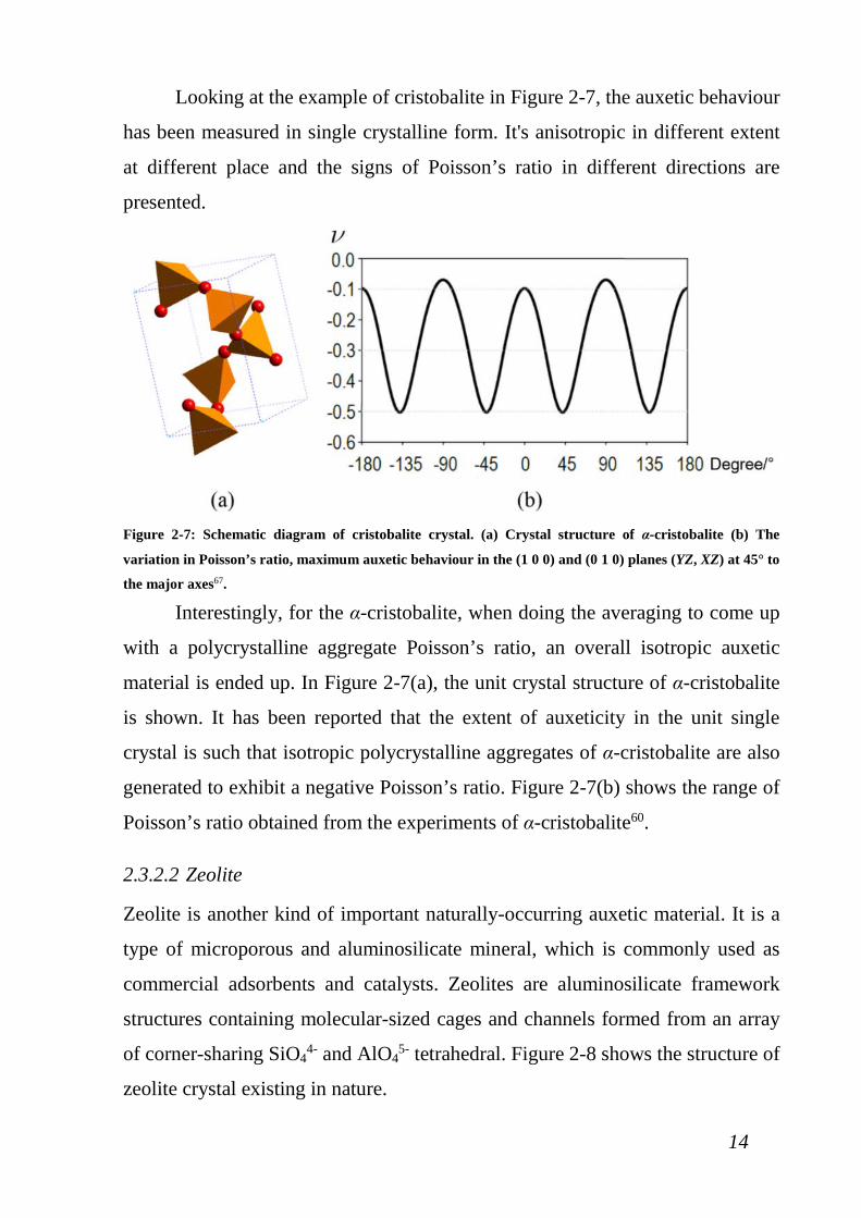
Looking at the example of cristobalite in Figure 2-7, the auxetic behaviour
has been measured in single crystalline form. It's anisotropic in different extent
at different place and the signs of Poisson’s ratio in different directions are
presented.
Figure 2-7: Schematic diagram of cristobalite crystal. (a) Crystal structure of α-cristobalite (b) The
variation in Poisson’s ratio, maximum auxetic behaviour in the (1 0 0) and (0 1 0) planes (YZ, XZ) at 45° to
the major axes67.
Interestingly, for the α-cristobalite, when doing the averaging to come up
with a polycrystalline aggregate Poisson’s ratio, an overall isotropic auxetic
material is ended up. In Figure 2-7(a), the unit crystal structure of α-cristobalite
is shown. It has been reported that the extent of auxeticity in the unit single
crystal is such that isotropic polycrystalline aggregates of α-cristobalite are also
generated to exhibit a negative Poisson’s ratio. Figure 2-7(b) shows the range of
Poisson’s ratio obtained from the experiments of α-cristobalite60.
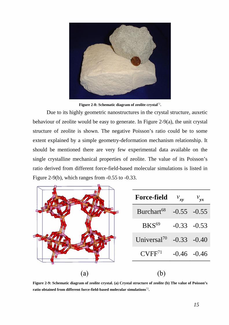
2.3.2.2 Zeolite
Zeolite is another kind of important naturally-occurring auxetic material. It is a
type of microporous and aluminosilicate mineral, which is commonly used as
commercial adsorbents and catalysts. Zeolites are aluminosilicate framework
structures containing molecular-sized cages and channels formed from an array
of corner-sharing SiO44- and AlO4
5- tetrahedral. Figure 2-8 shows the structure of
zeolite crystal existing in nature.
15
Figure 2-8: Schematic diagram of zeolite crystal72.
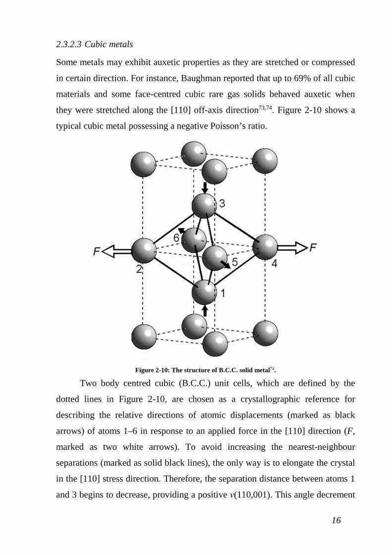
Due to its highly geometric nanostructures in the crystal structure, auxetic
behaviour of zeolite would be easy to generate. In Figure 2-9(a), the unit crystal
structure of zeolite is shown. The negative Poisson’s ratio could be to some
extent explained by a simple geometry-deformation mechanism relationship. It
should be mentioned there are very few experimental data available on the
single crystalline mechanical properties of zeolite. The value of its Poisson’s
ratio derived from different force-field-based molecular simulations is listed in
Figure 2-9(b), which ranges from -0.55 to -0.33.
Figure 2-9: Schematic diagram of zeolite crystal. (a) Crystal structure of zeolite (b) The value of Poisson’s
ratio obtained from different force-field-based molecular simulations72.
Force-field νxy νyx
Burchart68 -0.55 -0.55
BKS69 -0.33 -0.53
Universal70 -0.33 -0.40
CVFF71 -0.46 -0.46
16
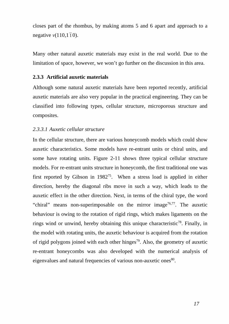
2.3.2.3 Cubic metals
Some metals may exhibit auxetic properties as they are stretched or compressed
in certain direction. For instance, Baughman reported that up to 69% of all cubic
materials and some face-centred cubic rare gas solids behaved auxetic when
they were stretched along the [110] off-axis direction73,74. Figure 2-10 shows a
typical cubic metal possessing a negative Poisson’s ratio.
Figure 2-10: The structure of B.C.C. solid metal74.
Two body centred cubic (B.C.C.) unit cells, which are defined by the
dotted lines in Figure 2-10, are chosen as a crystallographic reference for
describing the relative directions of atomic displacements (marked as black
arrows) of atoms 1–6 in response to an applied force in the [110] direction (F,
marked as two white arrows). To avoid increasing the nearest-neighbour
separations (marked as solid black lines), the only way is to elongate the crystal
in the [110] stress direction. Therefore, the separation distance between atoms 1
and 3 begins to decrease, providing a positive ν(110,001). This angle decrement
17
closes part of the rhombus, by making atoms 5 and 6 apart and approach to a
negative ν(110,1 1 0).
Many other natural auxetic materials may exist in the real world. Due to the
limitation of space, however, we won’t go further on the discussion in this area.
2.3.3 Artificial auxetic materials
Although some natural auxetic materials have been reported recently, artificial
auxetic materials are also very popular in the practical engineering. They can be
classified into following types, cellular structure, microporous structure and
composites.
2.3.3.1 Auxetic cellular structure
In the cellular structure, there are various honeycomb models which could show
auxetic characteristics. Some models have re-entrant units or chiral units, and
some have rotating units. Figure 2-11 shows three typical cellular structure
models. For re-entrant units structure in honeycomb, the first traditional one was
first reported by Gibson in 198275. When a stress load is applied in either
direction, hereby the diagonal ribs move in such a way, which leads to the
auxetic effect in the other direction. Next, in terms of the chiral type, the word
“chiral” means non-superimposable on the mirror image76,77. The auxetic
behaviour is owing to the rotation of rigid rings, which makes ligaments on the
rings wind or unwind, hereby obtaining this unique characteristic78. Finally, in
the model with rotating units, the auxetic behaviour is acquired from the rotation
of rigid polygons joined with each other hinges79. Also, the geometry of auxetic
re-entrant honeycombs was also developed with the numerical analysis of
eigenvalues and natural frequencies of various non-auxetic ones80.
18
Figure 2-11: Three typical cellular structure models81. A: Model with re-entrant units, B: Model with
chiral units, C: Model with rotating units. (a) Undeformed structure and (b) Deformed structure.
Due to its remarkable property and special microstructure, re-entrant
cellular units are adopted to achieve negative Poisson’s ratios of 2D materials in
this work.
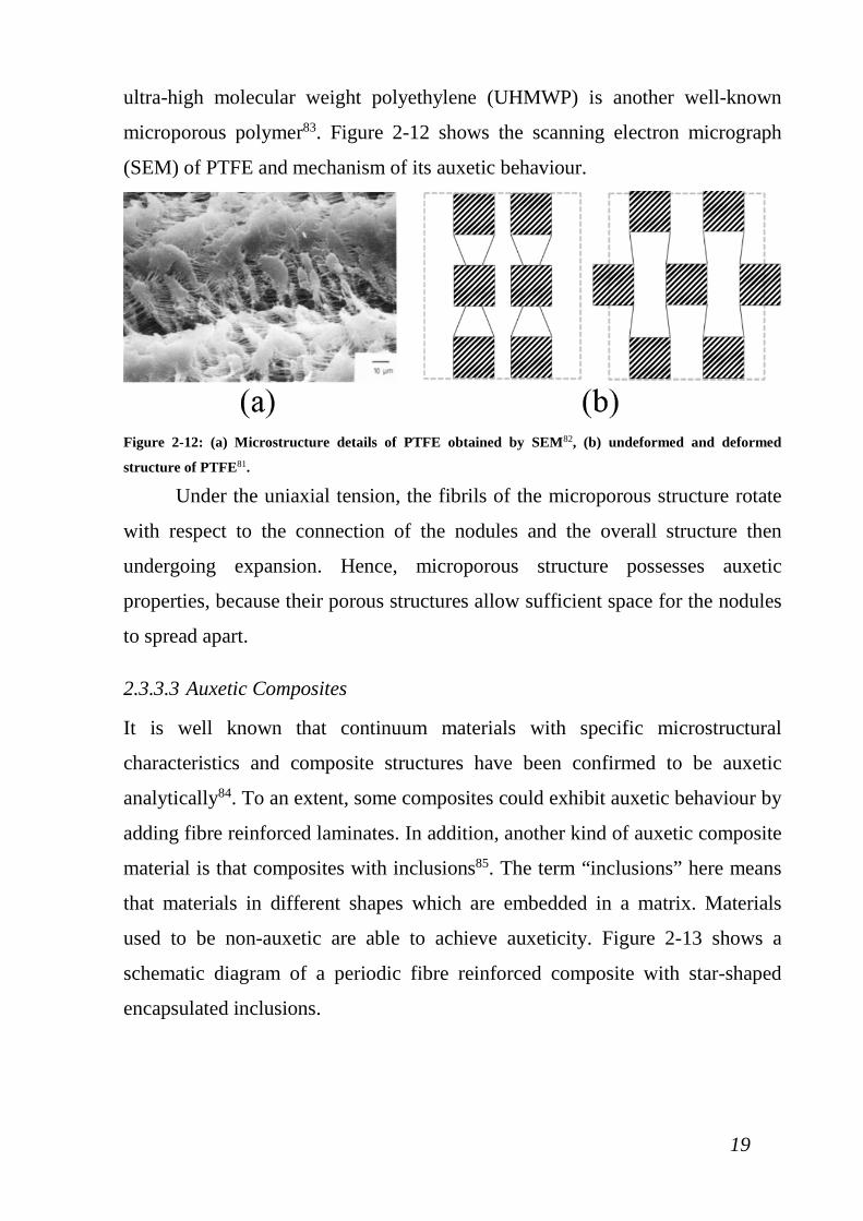
2.3.3.2 Auxetic microporous structure
Auxeticity in the microporous structure was first reported by Evans et al. in
1989, which is the expanded form of polytetrafluoroethylene (PTFE)82. Besides,
19
ultra-high molecular weight polyethylene (UHMWP) is another well-known
microporous polymer83. Figure 2-12 shows the scanning electron micrograph
(SEM) of PTFE and mechanism of its auxetic behaviour.
Figure 2-12: (a) Microstructure details of PTFE obtained by SEM82, (b) undeformed and deformed
structure of PTFE81.
Under the uniaxial tension, the fibrils of the microporous structure rotate
with respect to the connection of the nodules and the overall structure then
undergoing expansion. Hence, microporous structure possesses auxetic
properties, because their porous structures allow sufficient space for the nodules
to spread apart.
2.3.3.3 Auxetic Composites
It is well known that continuum materials with specific microstructural
characteristics and composite structures have been confirmed to be auxetic
analytically84. To an extent, some composites could exhibit auxetic behaviour by
adding fibre reinforced laminates. In addition, another kind of auxetic composite
material is that composites with inclusions85. The term “inclusions” here means
that materials in different shapes which are embedded in a matrix. Materials
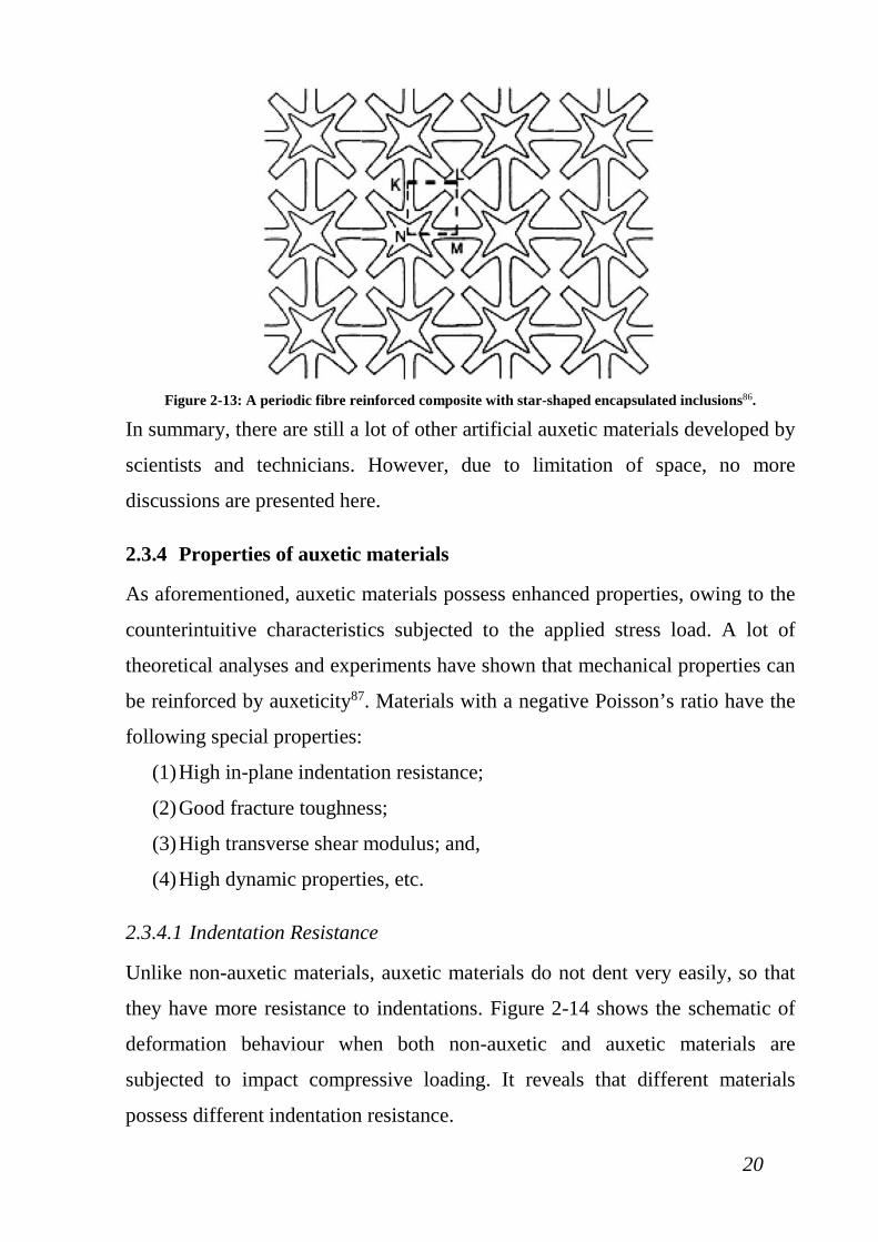
used to be non-auxetic are able to achieve auxeticity. Figure 2-13 shows a
schematic diagram of a periodic fibre reinforced composite with star-shaped
encapsulated inclusions.
20
Figure 2-13: A periodic fibre reinforced composite with star-shaped encapsulated inclusions86.
In summary, there are still a lot of other artificial auxetic materials developed by
scientists and technicians. However, due to limitation of space, no more
discussions are presented here.
2.3.4 Properties of auxetic materials
As aforementioned, auxetic materials possess enhanced properties, owing to the
counterintuitive characteristics subjected to the applied stress load. A lot of
theoretical analyses and experiments have shown that mechanical properties can
be reinforced by auxeticity87. Materials with a negative Poisson’s ratio have the
following special properties:
(1) High in-plane indentation resistance;
(2) Good fracture toughness;
(3) High transverse shear modulus; and,
(4) High dynamic properties, etc.
2.3.4.1 Indentation Resistance
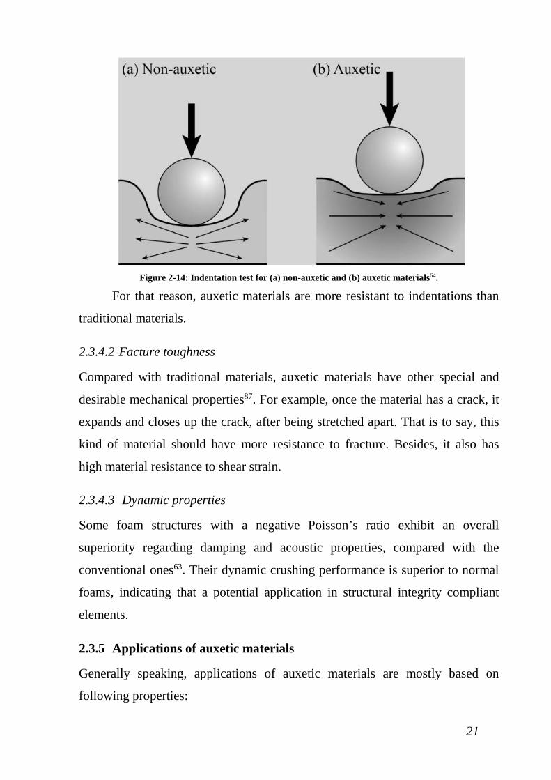
Unlike non-auxetic materials, auxetic materials do not dent very easily, so that
they have more resistance to indentations. Figure 2-14 shows the schematic of
deformation behaviour when both non-auxetic and auxetic materials are
subjected to impact compressive loading. It reveals that different materials
possess different indentation resistance.
21
Figure 2-14: Indentation test for (a) non-auxetic and (b) auxetic materials64.
For that reason, auxetic materials are more resistant to indentations than
traditional materials.
2.3.4.2 Facture toughness
Compared with traditional materials, auxetic materials have other special and
desirable mechanical properties87. For example, once the material has a crack, it
expands and closes up the crack, after being stretched apart. That is to say, this
kind of material should have more resistance to fracture. Besides, it also has
high material resistance to shear strain.
2.3.4.3 Dynamic properties
Some foam structures with a negative Poisson’s ratio exhibit an overall
superiority regarding damping and acoustic properties, compared with the
conventional ones63. Their dynamic crushing performance is superior to normal
foams, indicating that a potential application in structural integrity compliant
elements.
2.3.5 Applications of auxetic materials
Generally speaking, applications of auxetic materials are mostly based on
following properties:
22
(1) Unique negative Poisson’s ratios;
(2) Superior mechanical properties; and
(3) Acoustic absorption properties.
The Poisson’s ratio affects deformation kinematics in various ways, some of
them are useful and could influence the distribution of stress.
2.3.5.1 Sensors
Since the low bulk modulus of auxetic materials makes them more sensitive to
hydrostatic pressure, they can be adopted in the design of hydrophones or other
precision sensors. Due to the high in-plane indentation resistance, the sensitivity
of sensor made by auxetic materials is increased by almost one order of
magnitude, compared with traditional ones88.
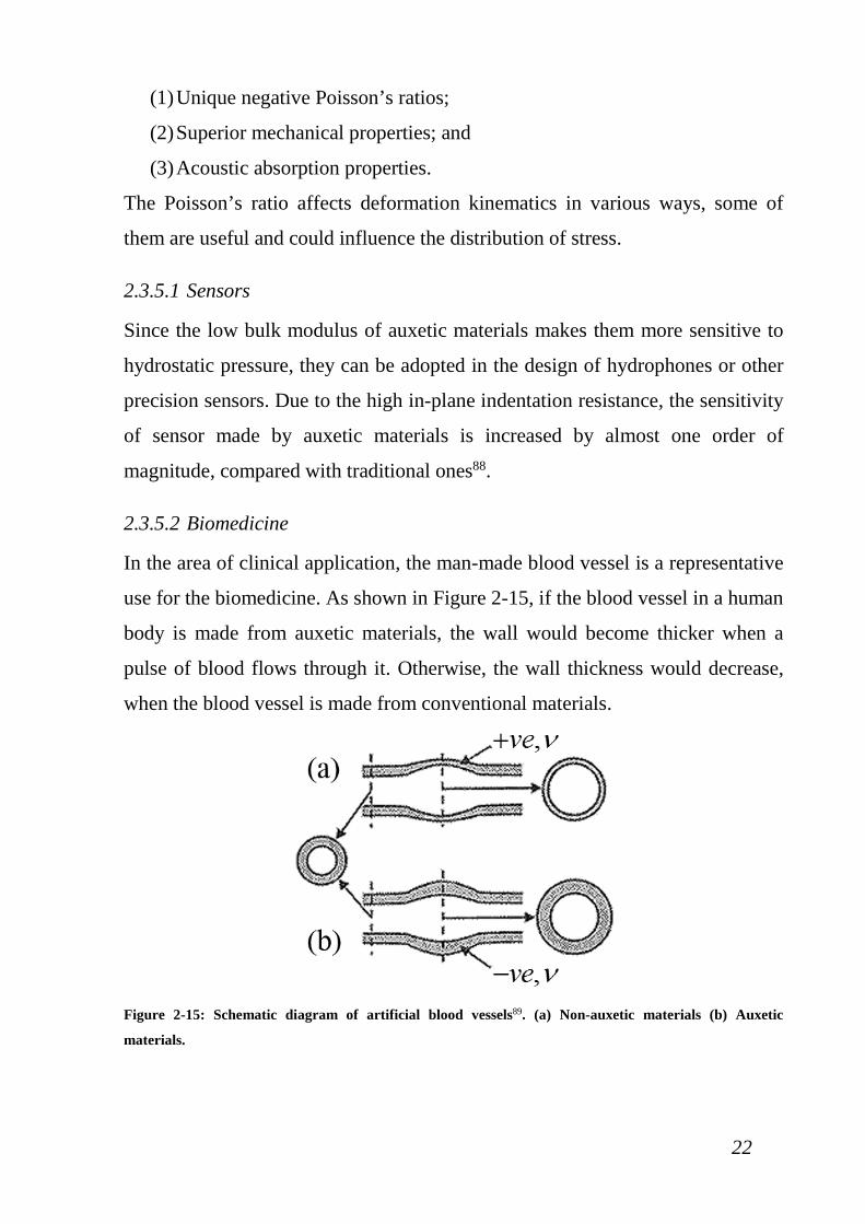
2.3.5.2 Biomedicine
In the area of clinical application, the man-made blood vessel is a representative
use for the biomedicine. As shown in Figure 2-15, if the blood vessel in a human
body is made from auxetic materials, the wall would become thicker when a
pulse of blood flows through it. Otherwise, the wall thickness would decrease,
when the blood vessel is made from conventional materials.
Figure 2-15: Schematic diagram of artificial blood vessels89. (a) Non-auxetic materials (b) Auxetic
materials.
23
Besides, some more potential applications, such as surgical implants90, and
suture anchors or muscle/ligament anchors, where the porous structure could
contribute to promoting bone growth89.
2.3.5.3 Aerospace and defence
Some structures with the unique properties of auxetic materials (i.e. negative
Poisson’s ratio) have already been adopted in real military defense applications.
For example, a kind of pyrolytic graphite (ν=-0.21) has been employed for
thermal protection in aerospace area91. And some large single crystals of Ni3Al
(νmin=-0.18) has been used in Vanessa for aircraft gas turbine engines74.
2.4 SUMMARY
To sum up, in this chapter, an in-depth summary of previous studies related to
this work is presented. Inspiring from their essence and discarding the dross, an
innovative idea of this thesis is proposed. For better studying the auxetic
kirigami made of 2D materials, an intensive study of 2D materials and auxetic
materials is also discussed here to help comprehend their characteristics and
applications.
24
Chapter 3 Research Methodology
In nano length scale, since the walls becoming more dominant, the classical
continuum mechanics theory breaks down gradually. Besides, due to the huge
consumption in experiments, there are still a lot of important questions remain
unsolved. Thus, the numerical simulation may provide an alternative approach
that could help to circumvent these problems. MD simulation is the most
common method for the study of mechanical behaviour at the nanoscale because
of relatively high accuracy, low computational cost92–94. Simulations at different
length scale considering different physics require different simulation methods.
To study the mechanical behaviour, MD simulation and molecular mechanics
are used to calculate the mechanical deformation of different 2D materials.
3.1 MD SIMULATION
In recent years, computational engineering have been extensively developed for
different length scales and material properties. In this work, the length scale
spans from nano to macro, and MD simulation is one of the most powerful tools
for computational mechanics study. MD simulation was first introduced by
Berni Alder for transition problem in 195792, and afterwards it was developed
for various studies in physics, biology, chemistry, material science and nano-
mechanics. MD computes time evolution of a cluster of interacting atoms by
integrating their equations of motions. The classical molecular dynamics is
employed here, and the word “classical” represents particles in simulation
system respects the classical mechanics, in other words, Newton’s Laws95, are
followed:
,i im=iF a (3.1)
For the atom i in a N-atom-system, where mi is the atom’s mass,
2
2 ,ii
ddt
=ra (3.2)
25
The term ai is the acceleration, and Fi is the force acting on the atom. Thus and
so, the force is derived as the gradients of potential with respect to atomic
displacements:
( )1, .ii NV= −∇rF r r (3.3)
Therefore, MD simulation is a deterministic method: given initial
positions and velocities, the Fi following time evolution is completely
determined and the computer calculates a trajectory in a 6N-dimensional phase
space (3N positions and 3N momenta). Besides, the MD simulation is a type of
statistical mechanics method which contains a set of distributions according to
determined statistical ensembles. Physical quantities could be easily evaluated
by taking the arithmetic average among different instantaneous values during the
MD simulation. In the limit of long simulation time, the phase space could be
regarded as fully sampled, and all the mechanical properties would be generated
during the averaging process. In summary, the MD simulation can be applied in
to calculate mechanical properties of microstructure made of different 2D
materials.
3.1.1 Modelling the N-atom physical system
The major part of a MD simulation is the physical model, which means selecting
the potential in simulation: a function, V(r1,…,rN). Forces are then derived from
the equation(3.3), which implies the conservation of total energy, and term V has
been simply written as a sum of pairwise interactions.
When it comes to the practical use, various types of many-body potentials
are now very popular in condensed matter simulation, because the
approximation has been recognized to be inadequate. The improvement of
discovering accurate potentials is remarkable, which includes the development
of Adaptive Intermolecular Reactive Empirical Bond Order (AIREBO)
potential96,97, Tersoff potential98–100 and Stillinger-Weber (SW) potential101,102,
etc. In this thesis, AIREBO potential is applied to the MD simulation about
carbon nanostructures; SW potential is employed to conduct MD simulation
26
related to single-layer MoS2; and Tersoff potential is involved in the MD
simulation on the single-layer h-BN.
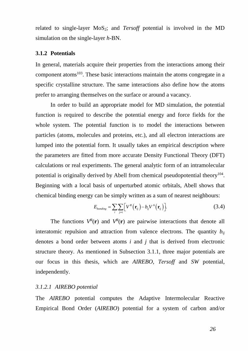
3.1.2 Potentials
In general, materials acquire their properties from the interactions among their
component atoms103. These basic interactions maintain the atoms congregate in a
specific crystalline structure. The same interactions also define how the atoms
prefer to arranging themselves on the surface or around a vacancy.
In order to build an appropriate model for MD simulation, the potential
function is required to describe the potential energy and force fields for the
whole system. The potential function is to model the interactions between
particles (atoms, molecules and proteins, etc.), and all electron interactions are
lumped into the potential form. It usually takes an empirical description where
the parameters are fitted from more accurate Density Functional Theory (DFT)
calculations or real experiments. The general analytic form of an intramolecular
potential is originally derived by Abell from chemical pseudopotential theory104.
Beginning with a local basis of unperturbed atomic orbitals, Abell shows that
chemical binding energy can be simply written as a sum of nearest neighbours:
( ) ( ) .R Abonding ij ij ij
i j iE V b V
≠
= − ∑∑ r r (3.4)
The functions VR(r) and VR(r) are pairwise interactions that denote all
interatomic repulsion and attraction from valence electrons. The quantity bij
denotes a bond order between atoms i and j that is derived from electronic
structure theory. As mentioned in Subsection 3.1.1, three major potentials are
our focus in this thesis, which are AIREBO, Tersoff and SW potential,
independently.
3.1.2.1 AIREBO potential
The AIREBO potential computes the Adaptive Intermolecular Reactive
Empirical Bond Order (AIREBO) potential for a system of carbon and/or
27
hydrogen atoms96. The AIREBO potential consists of three terms and could be
written as:
, , ,
1 .2
REBO LJ TORSIONij ij ijkl
i j i k i j l i j kE E E E
≠ ≠ ≠
= + +
∑∑ ∑ ∑ (3.5)
All of three terms are included in the simulation by default. The EREBO
term gives the model its reactive capabilities and only describes short-ranged C-
C, C-H and H-H interactions. The EREBO term adds longer-ranged interactions by
using a form similar to the standard Leonardo Jones potential. And the cutoff of
C-C is 0.34 nm, with a scale factor of 3.0, the resulting ELJ cutoff would be
1.02nm. The ETORSION term denotes an explicit 4-body potential that describes
various dihedral angle preferences in hydrocarbon configurations.
3.1.2.2 Tersoff potential
The Tersoff potential computes 3-body potential and its analytical form for the
pair potential:
( ) ( ) ( )
12
,
iji j i
ij C ij R ij ij A ij
E V
V f f b f
≠
=
= +
∑∑
r r r (3.6)
where the function fC(r) denotes a cutoff term, which ensures only nearest-
neighbour interactions, functions fR(r) and fA(r) are competing attractive and
repulsive pairwise terms, describes the 2-body interaction and the 3-body
interaction respectively. In addition, quantity bij is the bond angle term. The
hybrid B-N-C Tersoff potential105 is adopted in this thesis. More details of this
potential refer to Appendix A.
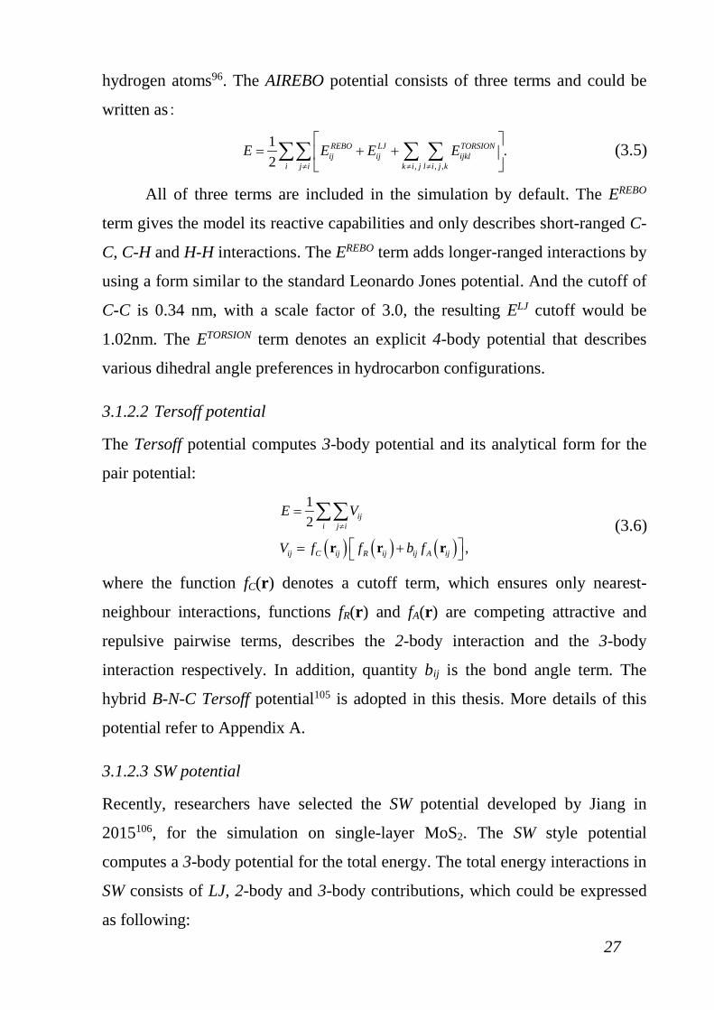
3.1.2.3 SW potential
Recently, researchers have selected the SW potential developed by Jiang in
2015106, for the simulation on single-layer MoS2. The SW style potential
computes a 3-body potential for the total energy. The total energy interactions in
SW consists of LJ, 2-body and 3-body contributions, which could be expressed
as following:
28
,total LJ two threeE E E E= + + (3.7)
where the Etwo term denotes all 2-body interactions with all possible pairs, i.e.
Mo-S, Mo-Mo and S-S:
( ) ( )max/ 4/ 1 ,r rtwoE Ae B rρ − = − (3.8)
And Ethree term covers the atoms involved in the ϕ, θ and ψ angles:
( ) ( ) ( )1 12 max12 2 13 max13 2/ /0cos cos .r r r r
threeE Ke ρ ρ θ θ − + − = − (3.9)
It is noted that the ELJ only takes effect when there are two or more layers
of MoS2 in simulation models and it denotes the van der Waals interaction
between S atoms in a different layer of multilayers MoS2. More details of this
potential refer to Appendix A.
3.1.3 Time integration algorithm
It is well known that the time integration algorithm is the most powerful
numerical method to integrate the equations of motion of the various interacting
particles and following their trajectory. The basic theory of time integration
algorithm is finite difference methods, where time is discretised on finite small
time step, ∆t. Once the positions, velocities and accelerations of particles are
given, the integration algorithm could derive all of these quantities at the later
time.
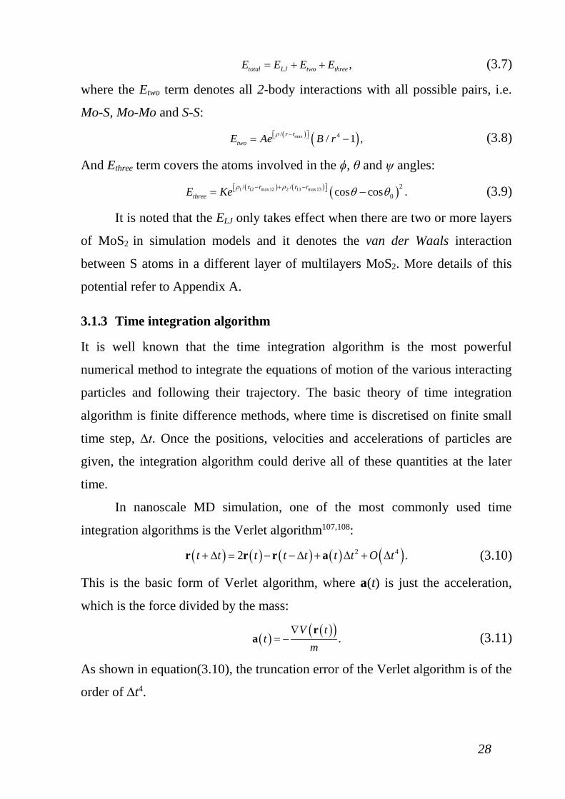
In nanoscale MD simulation, one of the most commonly used time
integration algorithms is the Verlet algorithm107,108:
( ) ( ) ( ) ( ) ( )2 42 .t t t t t t t O t+ ∆ = − −∆ + ∆ + ∆r r r a (3.10)
This is the basic form of Verlet algorithm, where a(t) is just the acceleration,
which is the force divided by the mass:
( ) ( )( ).
V tt
m∇
= −r
a (3.11)
As shown in equation(3.10), the truncation error of the Verlet algorithm is of the
order of ∆t4.
29
Despite the fact that algorithm is simple in use, as well as it is very
accurate and stable in the simulation, the problem with this kind of version is
that velocities are not generated directly. To eliminate this weakness, a better
version of the same algorithm is developed, named the velocity Verlet
algorithm. In this version of the algorithm, the positions, velocities and
accelerations at time t+∆t are derived from the same quantities at the time t as
following:
( ) ( ) ( ) ( )
( ) ( )
( ) ( )( )
( ) ( )
21 ,2
1 ,2 2
1 ,
1 .2 2
t t t t t a t t
tt t t t t
t t V t tm
tt t t t t t
+ ∆ = + ∆ + ∆
∆ + = ∆ + ∆
+ ∆ = − ∇ + ∆
∆ + ∆ = + + + ∆ ∆
r r v
r v a
a r
v v a
(3.12)
It is noted that if one wants to save 3N positions, velocities and
accelerations, 9N memory is occupied, but there is no need to simultaneously
store the values at two different times.
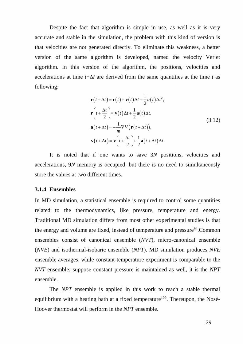
3.1.4 Ensembles
In MD simulation, a statistical ensemble is required to control some quantities
related to the thermodynamics, like pressure, temperature and energy.
Traditional MD simulation differs from most other experimental studies is that
the energy and volume are fixed, instead of temperature and pressure94.Common
ensembles consist of canonical ensemble (NVT), micro-canonical ensemble
(NVE) and isothermal-isobaric ensemble (NPT). MD simulation produces NVE
ensemble averages, while constant-temperature experiment is comparable to the
NVT ensemble; suppose constant pressure is maintained as well, it is the NPT
ensemble.
The NPT ensemble is applied in this work to reach a stable thermal
equilibrium with a heating bath at a fixed temperature109. Thereupon, the Nosé-
Hoover thermostat will perform in the NPT ensemble.
30
3.1.5 Energy minimization
In the field of MD simulation, energy minimization is the process of discovering
a stable arrangement in space of a congregation of atoms, according to the
second law thermodynamics. Performing an energy minimization of the
simulation system is to adjust atoms positions iteratively. The objective function
being minimized is the total potential energy of the system as a function of the
N-atom coordinates:
( ) ( ) ( ) ( )
( ) ( ) ( )
1, , , ,
, , , , , ,
, , , , ,
, , , , , , ,
N pair i j bond i j angle i j ki j i j i j k
angle i j k l improper i j k l fix ii j k l i j k l i
E E E E
E E E
= + + +
+ +
∑ ∑ ∑
∑ ∑ ∑
r r r r r r r r r
r r r r r r r r r
(3.13)
where the first term is the sum of non-bonded pairwise interactions, the second
to fifth terms are bond, angle, dihedral and improper interactions respectively,
and the last term is a supplementary term to equation.
Due to its high computational efficiency, Conjugate Gradient (CG)
algorithm often used in an atomistic simulation. Hence, CG algorithm is utilized
in this thesis for minimizing the whole simulation system110. The CG algorithm
mainly depends on the atomic forces and atomic energy. And it goes through a
series of search directions. The local minimum energy point along each search
direction is reached before algorithm proceeding to the next search.
3.1.6 Heating baths
The reliability of simulations significantly depends on an appropriate modelling
of the interaction with thermal reservoirs. In a study of the non-equilibrium
process, stationary non-equilibrium states are required to reach, by that to obtain
the relevant determined thermodynamic properties. In order to gain the stable
simulation, the reservoirs on both sides are linear, however, the central system is
nonlinear.
A conventional way to employ the interaction with reservoirs is to
introduce random forces and dissipation as stated in the fluctuation dissipation
31
theorem. Taking the case of one-dimension chain for example, this equals to the
following form of Langevin equations:
( ) ( ) ( ) ( )1 1 1 ,i i i i i i i i i iNm F F ξ λ δ ξ λ δ− + + + − −= − − − + − + −r r r r r r r (3.14)
where ξ+ and ξ- denote independent variables respecting Wiener processes with
zero mean and variance 2 BK Tλ± ± , KB is the Boltzmann constant and T± means the
temperature of two different heating reservoirs.
For the sake of providing a self-consistent description of out-of-
equilibrium processes, definitive heating baths have been introduced, among
which the Nosé-Hoover thermostat has been employed by most of researchers in
the MD simulation111,112.
In the heating bath, the evolution of the particles is controlled by the
following equation:
( ) ( )1 1
, i S,
, i Si
i i i i ii
m F Fςς+ +
− +− −
∈= − − − − ∈
rr r r r r
r
(3.15)
where ς± are supplementary variables which model the microscopic behaviours
of the thermostat, and S± stand for two sets of N± particles onto reservoirs.
3.1.7 Periodic boundary condition
The appropriate boundary condition is essential to the success of MD
simulation103. Fundamentally, the total number of atoms in an MD simulation is
usually up to many orders of magnitude smaller than required in most situations
of interest for materials simulation. By choosing the suitable periodic boundary
condition (PBC), one can mimic the effects of atoms outside the simulation box
and assist to remove the unwanted artefacts associated with the unavoidably
small size of simulation box. In a typical MD simulation, PBC could remove its
surface effects and maintain translational invariance. Usually, PBC could be
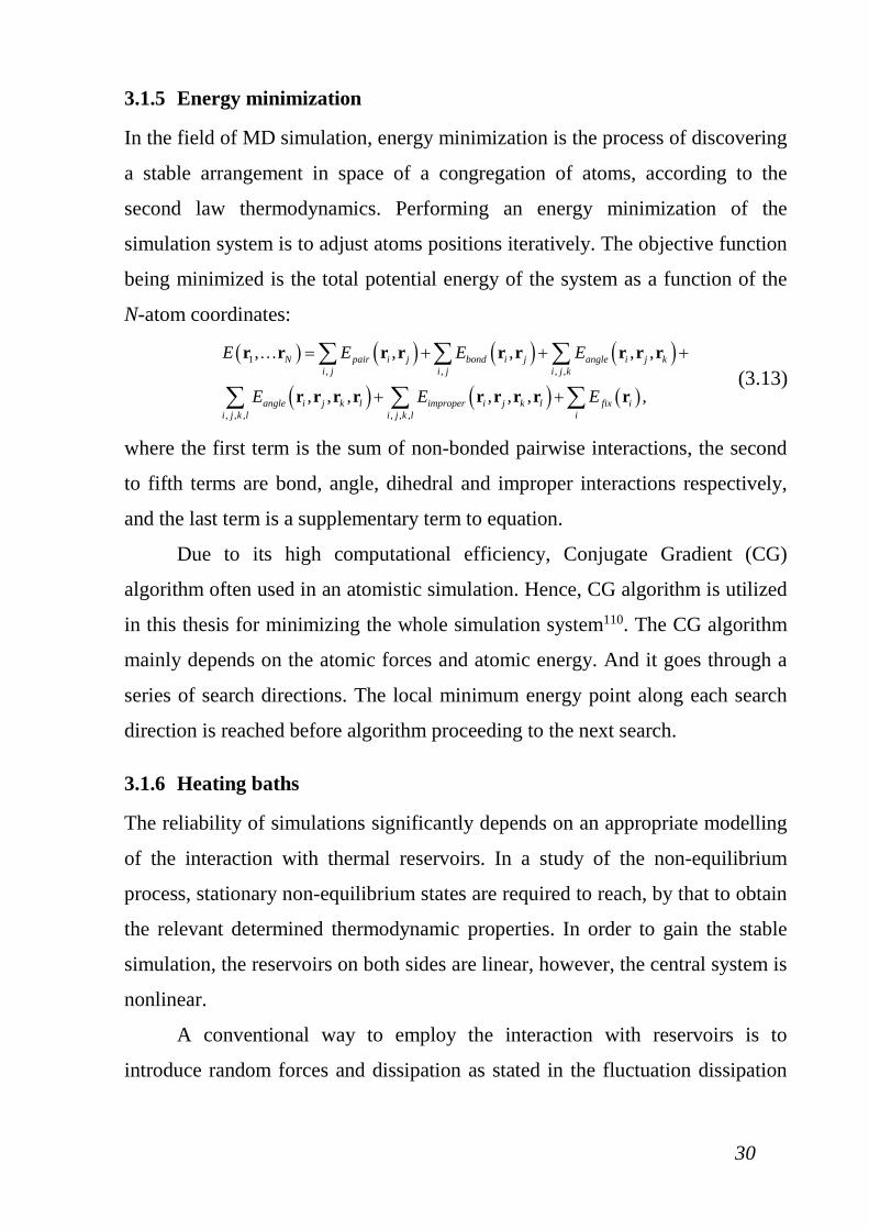
applied to one, two or three directions of simulation box. Figure 3-1 shows a
schematic diagram of PBC simulation box.
32
Figure 3-1: A schematic diagram of 3D PBC simulation box113.
3.1.8 MD software package
Nowadays, there are a lot of popular MD simulator software are implemented in
the research fields, such as LAMMPS, GROMACS, CHARMM, AMBER, NAMD
and MD++, etc.
In this work, MD simulations were conducted with the open source code
package LAMMPS. LAMMPS is a classical molecular dynamics code, and an
acronym for Large-scale Atomic/Molecular Massively Parallel Simulator114. It is
designed to be used for running efficiently on parallel computers. This kind of
simulator software package is distributed and developed by Sandia National
Laboratories, a US Department of Energy laboratory. It has potentials for solid-
state materials (metals, semiconductors) and soft matter (biomolecules,
polymers) and coarse-grained or mesoscopic systems, and could be used to
model atoms or, more generically, as a parallel particle simulator at the atomic
scale. To illustrate the procedure of MD simulation and structure of
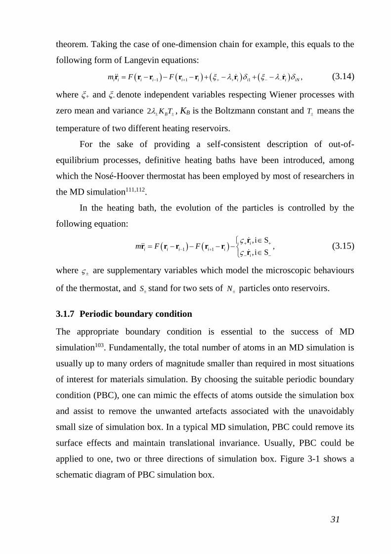
programming scripts simply and clearly, a flow chart is shown as in Figure 3-2.
33
Figure 3-2: A flow chart of MD simulation script programming.
3.2 STRAIN CALCULATION IN 2D MATERIAL KIRIGAMI
In this thesis, one of the most important mechanical quantities derived from MD
simulations is the strain calculation in 2D material kirigami. Based on the
continuum mechanics theory, there are two different methods were used to
calculate strain field of single-layer 2D material kirigami from atomistic
simulation results. The deformation control method and stress method are
discussed as followings.
3.2.1 Deformation control method
According to the continuum mechanics theory, uniaxial tensile tests are chosen
to obtain some essential mechanical properties. In the deformation control
34
method, the strain increment with a constant strain rate is applied to simulation
model every constant time step115.
In the uniaxial tensile test, the engineering (nominal) strain and stress are
related by the following equations:
0
0
,xt xx
x
L LL
ε −= (3.16)
0
0
,yt yy
y
L LL
ε−
= (3.17)
0
0 0 0
1
,
xx
x y
UV
V l l T
σε∂
=∂
= ⋅ ⋅ (3.18)
where lx0 and ly0 are the initial lengths of nanoribbon in x- and y-directions, lxt
and lyt are the lengths of the nanoribbon after deformation, term U denotes the
strain energy, term V0 is the initial volume of the simulation model and term T in
the equation means the assumed thickness of given 2D materials. Hence, the
equivalent Young’s modulus Eequiv and Poisson’s ratio ν are defined as follows:
2
20 0
1 ,x
equivx
UEV
εε
=
∂=
∂ (3.19)
.y
x
εν
ε= − (3.20)
In LAMMPS, the strain-control method is utilized by changing the volume
or shape of the simulation box during a dynamics run. Besides, engineering
strain rate could be maintained by using this method.
3.2.2 Stress method
In the MD simulations conducted on the LAMMPS, the virial stress could be
acquired on a per-atom basis. These stresses could then be derived to the strain
through a linear constitutive relationship116. In a stress plane model, the in-plane
strains could be written as:
35
( )
( )
1 ,
1 ,
.
xx xx yy
yy yy xx
xyxy
E
E
G
ε σ µσ
ε σ µσ
σε
= −
= −
=
(3.21)
However, it is noteworthy that, since the relationship between stress and
strain is assumed to be linear, then the resulting strain could be mostly
underestimated, especially at large deformation117.
The virial stress calculation consists of both potential and kinetic parts.
Moreover, the plane stress constitutive model was utilized to calculate the strain
by the equations of
1 0
1 0 ,
10 02
xx xx
yy yy
zz zz
E E
E E
G
µ
ε σµε σ
ε σ
− = − ⋅
(3.22)
It is noted that the values output from LAMMPS are in units of
“Pressure∙Volume”. Accordingly, the real value of stress should take the
“Volume” factor into calculation.
In general, the resultant strain is required in this research work, rather than
stress distribution. In addition, in order to better control and measure the rate of
applied stretched strain. The first method, which is deformation-control method,
is utilized here.
3.3 DENSITY FUNCTIONAL THEORY
Sometimes, the continuum mechanics theories become invalid to illustrate some
phenomenon at the nanoscale. To solve this problem, the density functional
theory (DFT) is introduced here, to investigate the electronic structure of atoms,
molecules and the condensed phases. By employing DFT, the properties of
nanostructure system could be determined by using the spatial electron density
contour. The electron density is the measurement of the probability of an
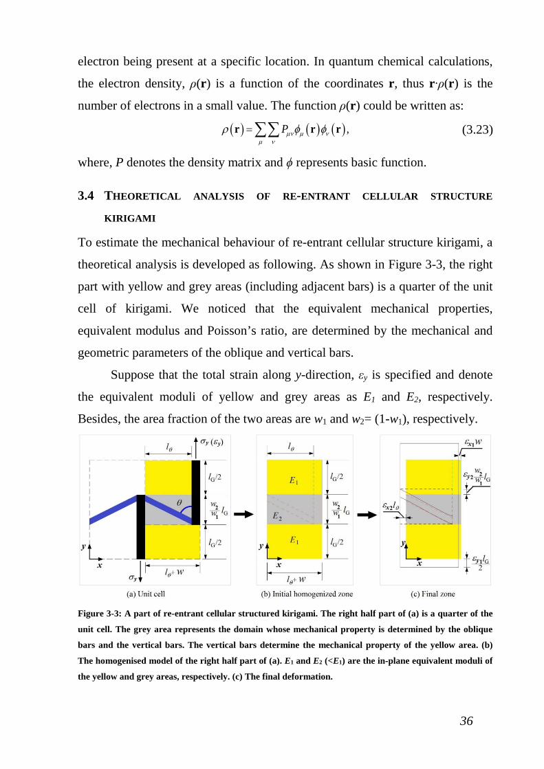
36
electron being present at a specific location. In quantum chemical calculations,
the electron density, ρ(r) is a function of the coordinates r, thus r∙ρ(r) is the
number of electrons in a small value. The function ρ(r) could be written as:
( ) ( ) ( ) ,Pµν µ νµ ν
ρ φ φ=∑∑r r r (3.23)
where, P denotes the density matrix and ϕ represents basic function.
3.4 THEORETICAL ANALYSIS OF RE-ENTRANT CELLULAR STRUCTURE
KIRIGAMI
To estimate the mechanical behaviour of re-entrant cellular structure kirigami, a
theoretical analysis is developed as following. As shown in Figure 3-3, the right
part with yellow and grey areas (including adjacent bars) is a quarter of the unit
cell of kirigami. We noticed that the equivalent mechanical properties,
equivalent modulus and Poisson’s ratio, are determined by the mechanical and
geometric parameters of the oblique and vertical bars.
Suppose that the total strain along y-direction, εy is specified and denote
the equivalent moduli of yellow and grey areas as E1 and E2, respectively.
Besides, the area fraction of the two areas are w1 and w2= (1-w1), respectively.
Figure 3-3: A part of re-entrant cellular structured kirigami. The right half part of (a) is a quarter of the
unit cell. The grey area represents the domain whose mechanical property is determined by the oblique
bars and the vertical bars. The vertical bars determine the mechanical property of the yellow area. (b)
The homogenised model of the right half part of (a). E1 and E2 (<E1) are the in-plane equivalent moduli of
the yellow and grey areas, respectively. (c) The final deformation.

37
The structure shown in Figure 3-3(b) could be further simplified as the structure
shown in Figure 3-4.
Figure 3-4: Simplified homogenized zone.
According to the composite materials theory118, the equivalent modulus of
the kirigami could be easily obtained as
1 2
1 2
1 ,equiv
w wE E E
= + (3.24)
then the equivalent modulus could be represented by Eequiv=E1∙E2/(E1∙w2+E2∙w1).
Let εy1 and εy2 represent the line strains of the yellow and grey parts along y-
direction, respectively. εy could be then written as:
1 1 2 2 ,y y yw wε ε ε+ = (3.25)
and the total resultant force along y-direction applied to yellow and grey parts is
the same:,
1 1 2 2.y y yF E Eε ε= ⋅ = ⋅ (3.26)
Making use of equations (3.25) and (3.26), the εy1 and εy2 could be expressed in
terms of εy as:
1
1 2 1 2
22 1 2 1
1/
.1
/
y y
y y
w w E E
w w E E
ε ε
ε ε
= + ⋅ = + ⋅
(3.27)
Besides, line strain of the half part along x-direction, εx could also be calculated
via the equation(3.25),
38
1 2 ,x x xlw
l w l wθ
θ θ
ε ε ε= ⋅ + ⋅+ +
(3.28)
where εx<0 is the x-strain of the vertical bar adjacent to the yellow part, εx2
denotes the x-strain of the grey part. For the structure with small deformation, it
can be obtained using the following formulation,
22 2
1
cot .Gx y
lww lθ
ε ε θ≈ ⋅ ⋅ (3.29)
Therefore, the equivalent Poisson’s ratio could be written as
2 1
2 1 2 1
1 1~ cot .1 / /
x xp
y y
wRw l w w E E lθ θ
ε εθε ε
= − ≈ − ⋅ + + + ⋅
(3.30)
By employing the theoretical analysis developed in this section, the size
effect of re-entrant cellular structure kirigami could be illustrated clearly.
3.5 SUMMARY
In summary, MD simulations are conducted within the Sandia-developed open
source code LAMMPS114. The Verlet algorithm is used for simulation time
integration with a time step of 0.5fs, and different ensembles are applied to the
given physical situations. For the potential aspects, interactions between carbon
atoms are described by the AIREBO potential96 with a cutoff at 1.02nm, which
has been adopted to measure the mechanical properties of carbon-based
nanostructures119,120. And the force field to describe interactions between Mo
and S atoms is a modified version of SW potential developed by Jiang106, in
2015. Besides, the interactions between B and N atoms in h-BN are set to be B-
N-C Tersoff potential105. All the simulations are carried out at 8K with Nosé-
Hoover thermostat. The deformation-control method with the applied strain ratio
of 5%/fs is used to perform uniaxial tensile tests in MD simulations.
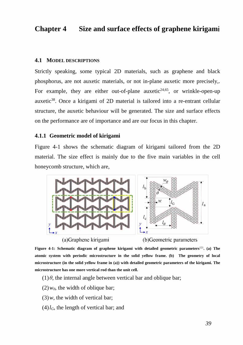
39
Chapter 4 Size and surface effects of graphene kirigami
4.1 MODEL DESCRIPTIONS
Strictly speaking, some typical 2D materials, such as graphene and black
phosphorus, are not auxetic materials, or not in-plane auxetic more precisely,.
For example, they are either out-of-plane auxetic24,65, or wrinkle-open-up
auxetic38. Once a kirigami of 2D material is tailored into a re-entrant cellular
structure, the auxetic behaviour will be generated. The size and surface effects
on the performance are of importance and are our focus in this chapter.
4.1.1 Geometric model of kirigami
Figure 4-1 shows the schematic diagram of kirigami tailored from the 2D
material. The size effect is mainly due to the five main variables in the cell
honeycomb structure, which are,
Figure 4-1: Schematic diagram of graphene kirigami with detailed geometric parameters121. (a) The
atomic system with periodic microstructure in the solid yellow frame. (b) The geometry of local
microstructure (in the solid yellow frame in (a)) with detailed geometric parameters of the kirigami. The
microstructure has one more vertical rod than the unit cell.
(1) θ, the internal angle between vertical bar and oblique bar;
(2) wθ, the width of oblique bar;
(3) w, the width of vertical bar;
(4) lG, the length of vertical bar; and
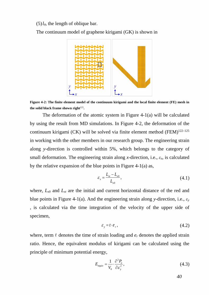
40
(5) lθ, the length of oblique bar.
The continuum model of graphene kirigami (GK) is shown in
Figure 4-2: The finite element model of the continuum kirigami and the local finite element (FE) mesh in
the solid black frame shown right121.
The deformation of the atomic system in Figure 4-1(a) will be calculated
by using the result from MD simulations. In Figure 4-2, the deformation of the
continuum kirigami (CK) will be solved via finite element method (FEM)122–125
in working with the other members in our research group. The engineering strain
along y-direction is controlled within 5%, which belongs to the category of
small deformation. The engineering strain along x-direction, i.e., εx, is calculated
by the relative expansion of the blue points in Figure 4-1(a) as,
0
0
,xt xx
x
L LL
ε−
= (4.1)
where, Lx0 and Lxt are the initial and current horizontal distance of the red and
blue points in Figure 4-1(a). And the engineering strain along y-direction, i.e., εy
, is calculated via the time integration of the velocity of the upper side of
specimen,
,y rt eε = ⋅ (4.2)
where, term t denotes the time of strain loading and er denotes the applied strain
ratio. Hence, the equivalent modulus of kirigami can be calculated using the
principle of minimum potential energy,
2
equiv 20 y
1 ,ePEV ε
∂= ⋅
∂ (4.3)
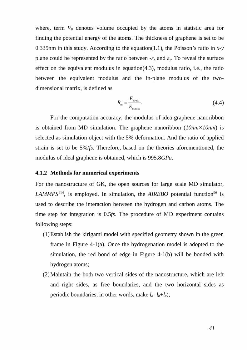
41
where, term V0 denotes volume occupied by the atoms in statistic area for
finding the potential energy of the atoms. The thickness of graphene is set to be
0.335nm in this study. According to the equation(1.1), the Poisson’s ratio in x-y
plane could be represented by the ratio between -εx and εy. To reveal the surface
effect on the equivalent modulus in equation(4.3), modulus ratio, i.e., the ratio
between the equivalent modulus and the in-plane modulus of the two-
dimensional matrix, is defined as
equivm
matrix
.E
RE
= (4.4)
For the computation accuracy, the modulus of idea graphene nanoribbon
is obtained from MD simulation. The graphene nanoribbon (10nm×10nm) is
selected as simulation object with the 5% deformation. And the ratio of applied
strain is set to be 5%/fs. Therefore, based on the theories aforementioned, the
modulus of ideal graphene is obtained, which is 995.8GPa.
4.1.2 Methods for numerical experiments
For the nanostructure of GK, the open sources for large scale MD simulator,
LAMMPS114, is employed. In simulation, the AIREBO potential function96 is
used to describe the interaction between the hydrogen and carbon atoms. The
time step for integration is 0.5fs. The procedure of MD experiment contains
following steps:
(1) Establish the kirigami model with specified geometry shown in the green
frame in Figure 4-1(a). Once the hydrogenation model is adopted to the
simulation, the red bond of edge in Figure 4-1(b) will be bonded with
hydrogen atoms;
(2) Maintain the both two vertical sides of the nanostructure, which are left
and right sides, as free boundaries, and the two horizontal sides as
periodic boundaries, in other words, make la=lb+lc);
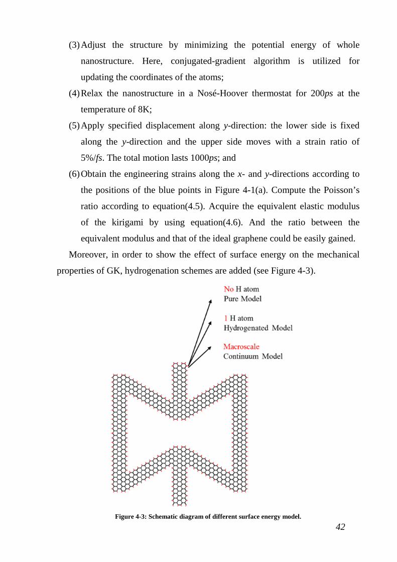
42
(3) Adjust the structure by minimizing the potential energy of whole
nanostructure. Here, conjugated-gradient algorithm is utilized for
updating the coordinates of the atoms;
(4) Relax the nanostructure in a Nosé-Hoover thermostat for 200ps at the
temperature of 8K;
(5) Apply specified displacement along y-direction: the lower side is fixed
along the y-direction and the upper side moves with a strain ratio of
5%/fs. The total motion lasts 1000ps; and
(6) Obtain the engineering strains along the x- and y-directions according to
the positions of the blue points in Figure 4-1(a). Compute the Poisson’s
ratio according to equation(4.5). Acquire the equivalent elastic modulus
of the kirigami by using equation(4.6). And the ratio between the
equivalent modulus and that of the ideal graphene could be easily gained.
Moreover, in order to show the effect of surface energy on the mechanical
properties of GK, hydrogenation schemes are added (see Figure 4-3).
Figure 4-3: Schematic diagram of different surface energy model.
43
If there is no carbon atom on the graphene bonded with the hydrogen atom, the
model is labelled as “+0H”; if each carbon atom on the edge (i.e., unsaturated
carbon atom) is bonded to a hydrogen atom, the model is labelled as “+1H”. The
potential energy and volume of the system with respect to the “+1H” model are
the summation of those of carbon atoms only. All the results will be compared
with those of a macrostructure with geometric similarity to the GK. The
Poisson’s ratio and the modulus ratio of the structure of CK are analysed by
finite element method. The analysis procedure of a deformed continuum using
FEM includes the following steps:
(1) Build the CK structure (shown in Figure 4-2) which has the same
geometric configuration with that of the GK;
(2) Mesh the CK structure with finite elements (plane stress elements);
(3) Add displacement constraints: the lower side is fixed along the y-
direction. The node located at the centre of the lower side is fully fixed.
Provide the nodes on the upper side of the structure with specified
displacement, which reflects the same engineering strain along the y-
direction, i.e., no more than 5%;
(4) Find the deformation of the CK structure by solving its equilibrium
equation; and
(5) Compute the Poisson’s ratio by using the displacement of the labelled
points in Figure 4-2. Obtain the modulus ratio by using equations (4.7)
and (4.8).
4.1.3 Schemes for size effect analysis
As shown in Figure 4-4, to study the size effect of the GK, the following
schemes are considered:

44
Figure 4-4: Configurations of the local microstructure of GK with different geometric parameters in five
schemes121. Here N(w) is denoted as the number of the basic honeycomb atoms along the direction of
variable w, e.g., N(w)=3 in Figure 4-1(b). (a) Scheme 1, θ changes; (b) N(wθ) changes; (c) N(w) changes; (d)
N(lG) changes; (e) N(lθ) changes.
(1) Variation of θ: Set N(wθ)=3, N(w)=3, N(lG)=6, N(lθ)=12, N(la)=55. θ
changes from 30° to 60°, 90°, 120° and 150°. The local microstructures
are shown in Figure 4-4(a);
(2) Variation of N(wθ): Set θ =60°, N(w)=3, N(lθ)=12, N(la)=33. N(wθ) is
chosen from {2, 3, 4, 5, 6, 7}, and the related value of N(lG) is set to be
16, 14, 12, 10, 8 and 6, respectively. The local microstructures are shown
in Figure 4-4(b);
(3) Variation of w: Set θ=60°, N(wθ)=3, N(lG)=6, N(lθ)=12, N(la)=25. N(w) is
chosen from {1, 3, 5, 7}. The local microstructures are shown in Figure
4-4(c);
(4) Variation of lG: Set θ=60°, N(wθ)=3, N(w) =3, N(lθ)=12. N(lG) is chosen
from {6, 12, 18, 24, 30, 36}, which leads N(la) equal to 25, 31, 37, 43, 49
and 55, respectively. The local microstructures are shown in Figure
4-4(d); and
(5) Variation of lθ: Set θ=60°, N(wθ)=3, N(w) =3, N(lG)=12. N(lθ) is chosen
from {12, 15, 18, 21, 24, 27}, which makes N(la) equal 25, 28, 31, 34, 37

45
and 40, correspondingly. The local microstructures are shown in Figure
4-4(e).
4.2 NUMERICAL RESULTS AND DISCUSSIONS
4.2.1 Results on included angle between vertical and oblique bar varying
In the first scheme, θ is chosen from the angles, i.e., 30, 60, 90, 120 and 150
degrees, respectively. The other parameters are given in Subsection 4.1.3. The
Poisson’s ratio and the modulus ratio are calculated using MD and FEM
simulations, and the results are shown in Table 4-1. Table 4-1: Comparisons of Poisson’s ratio and the modulus ratio for the three models in Scheme 1.
θ =30° θ =60° θ =90° θ =120° θ =150° Rp (GK+0H) -2.074 -0.980 0.318 1.868 6.302 Rp (GK+1H) -1.442 -0.669 0.149 1.667 5.077 Rp (CK) -1.139 -0.722 0.035 1.034 2.907
Rm (GK+0H) 5.16% 14.40% 17.91% 23.14% 31.27% Rm (GK+1H) 7.08% 16.86% 22.31% 25.63% 37.91% Rm (CK) 1.88% 2.05% 2.19% 2.59% 4.47%
Table 4-1 lists the Poisson’s ratios and modulus ratios of the GK with
different values of θ. For the Poisson’s ratio of GK in the three models, the
value increases monotonously along with an increase in θ. When θ is less than
90°, the Poisson’s ratio is negative, i.e., GK shows auxetic behaviour. At θ=90°,
the Poisson’s ratios are positive, rather than zero. The reason is that the oblique
bar, which currently is horizontal, has a rotary angle which leads to θ>90°. The
table also demonstrates the value of Rp is sensitive to the surface modification.
For example, for “+0H” model, Rp is 0.318, which is over twice of 0.149 of
“+1H” model, and is far greater than 0.035 of CK model. Similar differences
among the values of Rp of the three models can also be found at any other values
of θ. It is concluded that the GK without hydrogenation (+0H model) has the
highest absolute value of Rp among the three models. The hydrogenated GK
(+1H model) has a lower absolute value of Rp than the pure carbon kirigami
does, but the value is higher than that of the CK (calculated using FEM) if θ is
not 60°.
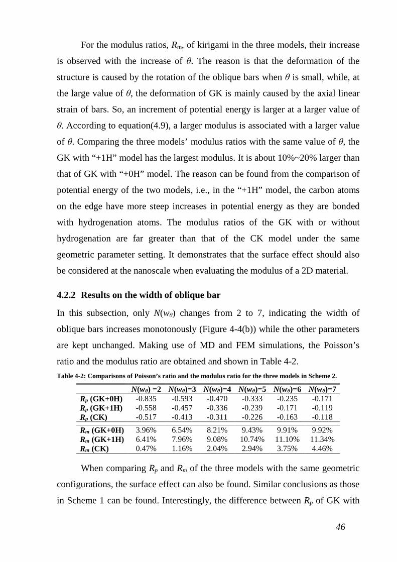
46
For the modulus ratios, Rm, of kirigami in the three models, their increase
is observed with the increase of θ. The reason is that the deformation of the
structure is caused by the rotation of the oblique bars when θ is small, while, at
the large value of θ, the deformation of GK is mainly caused by the axial linear
strain of bars. So, an increment of potential energy is larger at a larger value of
θ. According to equation(4.9), a larger modulus is associated with a larger value
of θ. Comparing the three models’ modulus ratios with the same value of θ, the
GK with “+1H” model has the largest modulus. It is about 10%~20% larger than
that of GK with “+0H” model. The reason can be found from the comparison of
potential energy of the two models, i.e., in the “+1H” model, the carbon atoms
on the edge have more steep increases in potential energy as they are bonded
with hydrogenation atoms. The modulus ratios of the GK with or without
hydrogenation are far greater than that of the CK model under the same
geometric parameter setting. It demonstrates that the surface effect should also
be considered at the nanoscale when evaluating the modulus of a 2D material.
4.2.2 Results on the width of oblique bar
In this subsection, only N(wθ) changes from 2 to 7, indicating the width of
oblique bars increases monotonously (Figure 4-4(b)) while the other parameters
are kept unchanged. Making use of MD and FEM simulations, the Poisson’s
ratio and the modulus ratio are obtained and shown in Table 4-2. Table 4-2: Comparisons of Poisson’s ratio and the modulus ratio for the three models in Scheme 2.
N(wθ) =2 N(wθ)=3 N(wθ)=4 N(wθ)=5 N(wθ)=6 N(wθ)=7 Rp (GK+0H) -0.835 -0.593 -0.470 -0.333 -0.235 -0.171 Rp (GK+1H) -0.558 -0.457 -0.336 -0.239 -0.171 -0.119 Rp (CK) -0.517 -0.413 -0.311 -0.226 -0.163 -0.118
Rm (GK+0H) 3.96% 6.54% 8.21% 9.43% 9.91% 9.92% Rm (GK+1H) 6.41% 7.96% 9.08% 10.74% 11.10% 11.34% Rm (CK) 0.47% 1.16% 2.04% 2.94% 3.75% 4.46% When comparing Rp and Rm of the three models with the same geometric
configurations, the surface effect can also be found. Similar conclusions as those
in Scheme 1 can be found. Interestingly, the difference between Rp of GK with
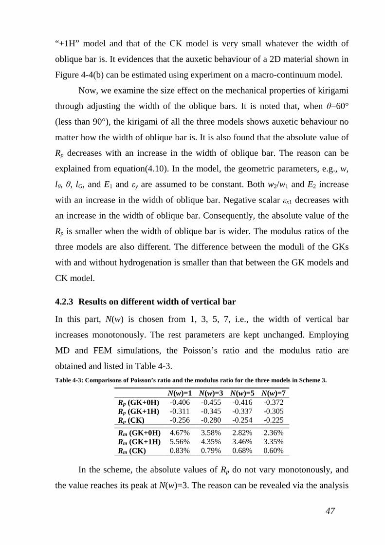
47
“+1H” model and that of the CK model is very small whatever the width of
oblique bar is. It evidences that the auxetic behaviour of a 2D material shown in
Figure 4-4(b) can be estimated using experiment on a macro-continuum model.
Now, we examine the size effect on the mechanical properties of kirigami
through adjusting the width of the oblique bars. It is noted that, when θ=60°
(less than 90°), the kirigami of all the three models shows auxetic behaviour no
matter how the width of oblique bar is. It is also found that the absolute value of
Rp decreases with an increase in the width of oblique bar. The reason can be
explained from equation(4.10). In the model, the geometric parameters, e.g., w,
lθ, θ, lG, and E1 and εy are assumed to be constant. Both w2/w1 and E2 increase
with an increase in the width of oblique bar. Negative scalar εx1 decreases with
an increase in the width of oblique bar. Consequently, the absolute value of the
Rp is smaller when the width of oblique bar is wider. The modulus ratios of the
three models are also different. The difference between the moduli of the GKs
with and without hydrogenation is smaller than that between the GK models and
CK model.
4.2.3 Results on different width of vertical bar
In this part, N(w) is chosen from 1, 3, 5, 7, i.e., the width of vertical bar
increases monotonously. The rest parameters are kept unchanged. Employing
MD and FEM simulations, the Poisson’s ratio and the modulus ratio are
obtained and listed in Table 4-3. Table 4-3: Comparisons of Poisson’s ratio and the modulus ratio for the three models in Scheme 3.
N(w)=1 N(w)=3 N(w)=5 N(w)=7 Rp (GK+0H) -0.406 -0.455 -0.416 -0.372 Rp (GK+1H) -0.311 -0.345 -0.337 -0.305 Rp (CK) -0.256 -0.280 -0.254 -0.225
Rm (GK+0H) 4.67% 3.58% 2.82% 2.36% Rm (GK+1H) 5.56% 4.35% 3.46% 3.35% Rm (CK) 0.83% 0.79% 0.68% 0.60%
In the scheme, the absolute values of Rp do not vary monotonously, and
the value reaches its peak at N(w)=3. The reason can be revealed via the analysis
48
using equation(4.11), for example, when N(w)=1, the width of vertical bar is less
than that of oblique bar, the vertical bar plays a major role in the deformation of
the GK. The rotary angle of the oblique bar is small because of small tension
component on the vertical bar (σy). As N(w)=3, the vertical bar has a stronger
tensile force which leads to a higher rotary angle of oblique bar. Therefore, the
Rp at N(w)=3 is larger than that at N(w)=1. When N(w)≥5, the rotary angle of
oblique bar is slightly larger than that at N(w)=3. Simultaneously, w/lθ is over
1.6 times of that at N(w)=3. From the second item in the left part of
equation(4.12), we can find that the wider width of the vertical bar (N(w)≥5)
leads to smaller Poisson’s ratio of the GK. On the other hand, the difference
between the Poisson’s ratio of GK with “+1H” model and CK model is obvious
no matter if θ=60° or not in the models. It implies that the surface effect cannot
be neglected when using the continuum model to estimate the auxetic behaviour
of GK with different widths of vertical bar.
For the modulus ratio of the three models, it decreases along with an
increase in the width of vertical bar. The reason is that the deformation of the
GK mainly depends on the rotation of the oblique bar during loading in y-
direction. Hence, the variation of potential energy of the vertical bar decreases
along with an increase in its width. Therefore, the variation of potential energy
of the system decreases, too, which results in decrease in the modulus according
to equation(4.13).
4.2.4 Results on different length of vertical bar
In this scheme, the length of vertical bar N(lG) is chosen from 6, 12, 18, 24, 30
and 36. The other parameters are maintained invariant. The results of Poisson’s
ratio and the modulus ratio obtained from MD and FEM simulations are listed in
Table 4-4.

49
Table 4-4: Comparisons of Poisson’s ratio and the modulus ratio for the three models in Scheme 4.
N(lG)=6 N(lG)=12 N(lG)=28 N(lG)=24 N(lG)=30 N(lG)=36 Rp (GK+0H) -0.455 -0.559 -0.662 -0.763 -0.845 -0.980 Rp (GK+1H) -0.345 -0.430 -0.505 -0.560 -0.623 -0.669 Rp (CK) -0.280 -0.381 -0.475 -0.563 -0.645 -0.722
Rm (GK+0H) 3.58% 5.71% 7.94% 9.97% 12.29% 14.40% Rm (GK+1H) 4.35% 6.93% 9.58% 11.93% 14.36% 16.86% Rm (CK) 0.79% 1.07% 1.34% 1.59% 1.82% 2.05%
When the length of vertical bar increases or N(lG) changes from 6 to 36,
the absolute values of Poisson’s ratio of the three models increase
monotonously. The reason can be found by checking either equation(4.14), or
the deformation of Figure 3-3(b). For example, for the second item of the left
part of equation(4.15), when w, lθ, E1 and E2(<E1), are kept constant, an increase
in w1 leads to the increase of Rp. It suggests that the 2D material can achieve
higher auxetic effect through use of longer vertical bars. In this scheme, the
difference between the values of Rp of the hydrogenated GK and CK model is
very small. One can estimate the auxetic behaviour of the GK using the
experiments on the continuum model with the same geometric configurations
according to this principle.
The modulus ratio of the three models increase with an increase in the
length of vertical bar. But the maximal value is reached when w1 tends to be 1.0.
The maximal value will be E1/Ematrix=w/(w+lθ)∙(Evert_bar/Ematrix)=~20%, according
to equations (4.16) and (4.17) and Figure 3-3(b). The hydrogenated GK still has
the highest modulus among the three models. The CK model has the lowest
modulus, which is no more than 20% of that of the hydrogenated GK.
4.2.5 Results on different length of oblique bar
At last, the change in the length of oblique bar are achieved by selecting
different N(lθ). In this work, N(lθ) is chosen from 12, 15, 18, 24 and 27. The
remaining parameters are kept constant. The corresponding results of Poisson’s
ratio and the modulus ratio are listed in Table 4-5.
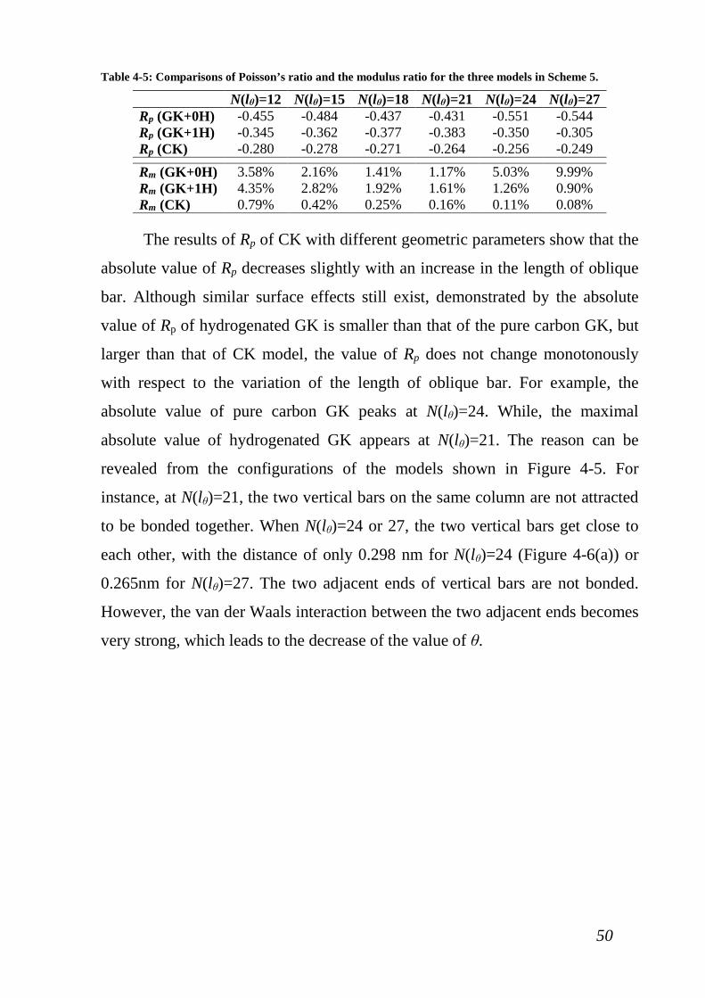
50
Table 4-5: Comparisons of Poisson’s ratio and the modulus ratio for the three models in Scheme 5.
N(lθ)=12 N(lθ)=15 N(lθ)=18 N(lθ)=21 N(lθ)=24 N(lθ)=27 Rp (GK+0H) -0.455 -0.484 -0.437 -0.431 -0.551 -0.544 Rp (GK+1H) -0.345 -0.362 -0.377 -0.383 -0.350 -0.305 Rp (CK) -0.280 -0.278 -0.271 -0.264 -0.256 -0.249
Rm (GK+0H) 3.58% 2.16% 1.41% 1.17% 5.03% 9.99% Rm (GK+1H) 4.35% 2.82% 1.92% 1.61% 1.26% 0.90% Rm (CK) 0.79% 0.42% 0.25% 0.16% 0.11% 0.08% The results of Rp of CK with different geometric parameters show that the
absolute value of Rp decreases slightly with an increase in the length of oblique
bar. Although similar surface effects still exist, demonstrated by the absolute
value of Rp of hydrogenated GK is smaller than that of the pure carbon GK, but
larger than that of CK model, the value of Rp does not change monotonously
with respect to the variation of the length of oblique bar. For example, the
absolute value of pure carbon GK peaks at N(lθ)=24. While, the maximal
absolute value of hydrogenated GK appears at N(lθ)=21. The reason can be
revealed from the configurations of the models shown in Figure 4-5. For
instance, at N(lθ)=21, the two vertical bars on the same column are not attracted
to be bonded together. When N(lθ)=24 or 27, the two vertical bars get close to
each other, with the distance of only 0.298 nm for N(lθ)=24 (Figure 4-6(a)) or
0.265nm for N(lθ)=27. The two adjacent ends of vertical bars are not bonded.
However, the van der Waals interaction between the two adjacent ends becomes
very strong, which leads to the decrease of the value of θ.
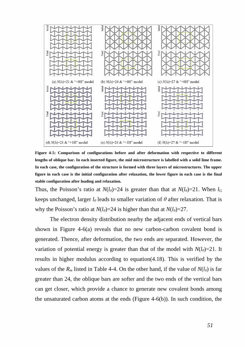
51
Figure 4-5: Comparison of configurations before and after deformation with respective to different
lengths of oblique bar. In each inserted figure, the mid microstructure is labelled with a solid lime frame.
In each case, the configuration of the structure is formed with three layers of microstructures. The upper
figure in each case is the initial configuration after relaxation, the lower figure in each case is the final
stable configuration after loading and relaxation.
Thus, the Poisson’s ratio at N(lθ)=24 is greater than that at N(lθ)=21. When lG
keeps unchanged, larger lθ leads to smaller variation of θ after relaxation. That is
why the Poisson’s ratio at N(lθ)=24 is higher than that at N(lθ)=27.
The electron density distribution nearby the adjacent ends of vertical bars
shown in Figure 4-6(a) reveals that no new carbon-carbon covalent bond is
generated. Thence, after deformation, the two ends are separated. However, the
variation of potential energy is greater than that of the model with N(lθ)=21. It
results in higher modulus according to equation(4.18). This is verified by the
values of the Rm listed in Table 4-4. On the other hand, if the value of N(lθ) is far
greater than 24, the oblique bars are softer and the two ends of the vertical bars
can get closer, which provide a chance to generate new covalent bonds among
the unsaturated carbon atoms at the ends (Figure 4-6(b)). In such condition, the
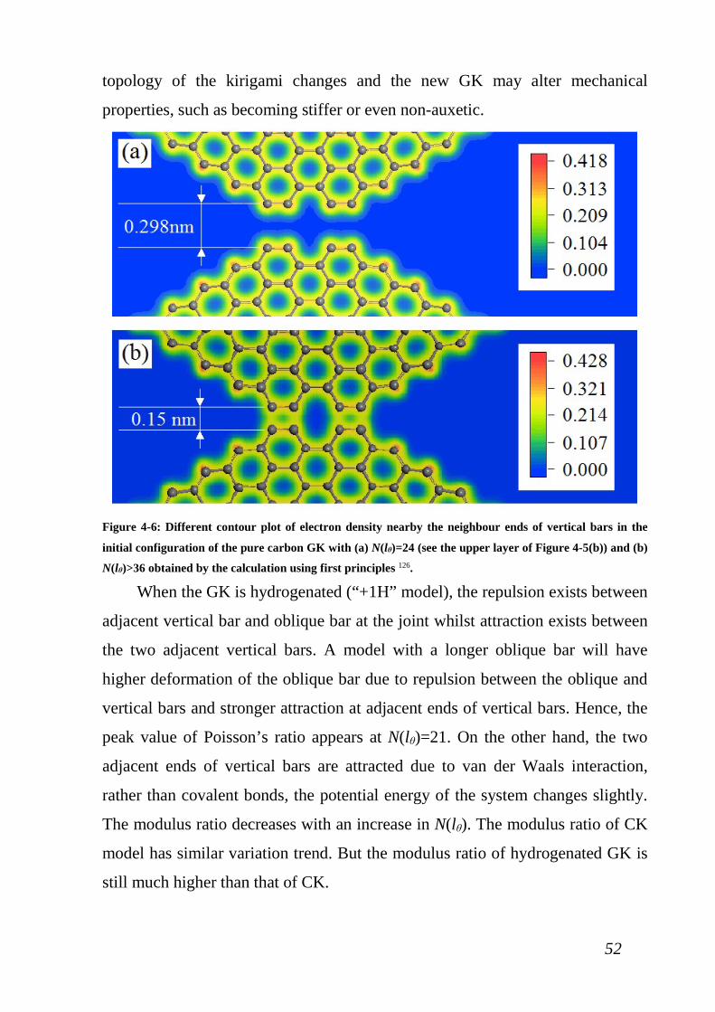
52
topology of the kirigami changes and the new GK may alter mechanical
properties, such as becoming stiffer or even non-auxetic.
Figure 4-6: Different contour plot of electron density nearby the neighbour ends of vertical bars in the
initial configuration of the pure carbon GK with (a) N(lθ)=24 (see the upper layer of Figure 4-5(b)) and (b)
N(lθ)>36 obtained by the calculation using first principles 126.
When the GK is hydrogenated (“+1H” model), the repulsion exists between
adjacent vertical bar and oblique bar at the joint whilst attraction exists between
the two adjacent vertical bars. A model with a longer oblique bar will have
higher deformation of the oblique bar due to repulsion between the oblique and
vertical bars and stronger attraction at adjacent ends of vertical bars. Hence, the
peak value of Poisson’s ratio appears at N(lθ)=21. On the other hand, the two
adjacent ends of vertical bars are attracted due to van der Waals interaction,
rather than covalent bonds, the potential energy of the system changes slightly.
The modulus ratio decreases with an increase in N(lθ). The modulus ratio of CK
model has similar variation trend. But the modulus ratio of hydrogenated GK is
still much higher than that of CK.
53
4.3 SUMMARY
In conclusion, after analysing the Poisson’s ratio and modulus ratio of GK with
re-entrant honeycomb microstructure, the dependence of the two mechanical
properties on the sizes of the microstructure is revealed. And the mechanical
response of the CK with geometric similarity to the GK is also calculated for
exploring the surface effect of GK through comparisons of the related responses.
The results show that the specified Poisson’s ratio and modulus of GK can be
obtained by adjusting the sizes of the microstructure. The results presented in
this chapter has been published in Nature Scientific Report127. Some conclusions
can be made as follows:
(1) Of all the schemes, pure carbon GK, being with the highest surface energy,
has the highest absolute value of Poisson’s ratio among the three models. The
absolute value of Poisson’s ratio of the hydrogenated GK is higher than that
of the CK due to the higher surface energy of the GK than that of the CK.
Regarding the effect of θ illustrated in scheme 1, when θ is less than 90°, GK
shows auxetic.
(2) In general, the modulus ratio of hydrogenated GK is about 10%~20% higher
than that of the pure carbon GK. The modulus ratio of CK is far less than that
of the GK when they have the same geometric configurations. It
demonstrates the significant surface effect on the modulus of 2D
nanomaterials.
(3) In Scheme 2, the difference between the Poisson’s ratios of hydrogenated GK
and CK models is very small, meaning that the Poisson’s ratios depend on
the width of oblique bar, slightly. It indicates that the auxetic behaviour of a
2D nanomaterial can be estimated using the experiment on a macro-
continuum model with respect to the width of oblique bar. For the modulus
ratios of GK and CK models, when the width of oblique bar increases, the
absolute value of Rp decreases, but the modulus ratio increases,
monotonically.
54
(4) When increasing the width of vertical bar as was done in scheme 3, the peak
value of Poisson’s ration appears at N(w)=3. The difference between the
Poisson’s ratios of GK models and CK model is obvious. As for the modulus
ratios of the three models, they decrease with an increase in the width of
vertical bar.
(5) When the length of vertical bar N(lG) increases from 6 to 36, the absolute
values of Poisson’s ratio of the three models increases monotonously. It
suggests that the 2D material can have higher auxetic effect with longer
vertical bars as illustrated in Scheme 4. In this condition, the difference
between the values of Poisson’s ratio of the hydrogenated GK and CK model
is very small. The auxetic behaviour of GK can be estimated using the
experiments on the CK model with the same geometric configurations. The
modulus ratio of the three models increases with an increase in the length of
vertical bar.
(6) In Scheme 5, the absolute value of Poisson’s ratio varies slightly with the
increase in the length of oblique bar (or N(lθ)). If the value of lG is small (i.e.,
vertical bars are short), the two adjacent vertical bars in pure carbon GK
model may be bonded together. It results in the sharp increase of both
Poisson’s ratio and modulus ratio. But it does not happen in either the
hydrogenated GK model or the CK model.
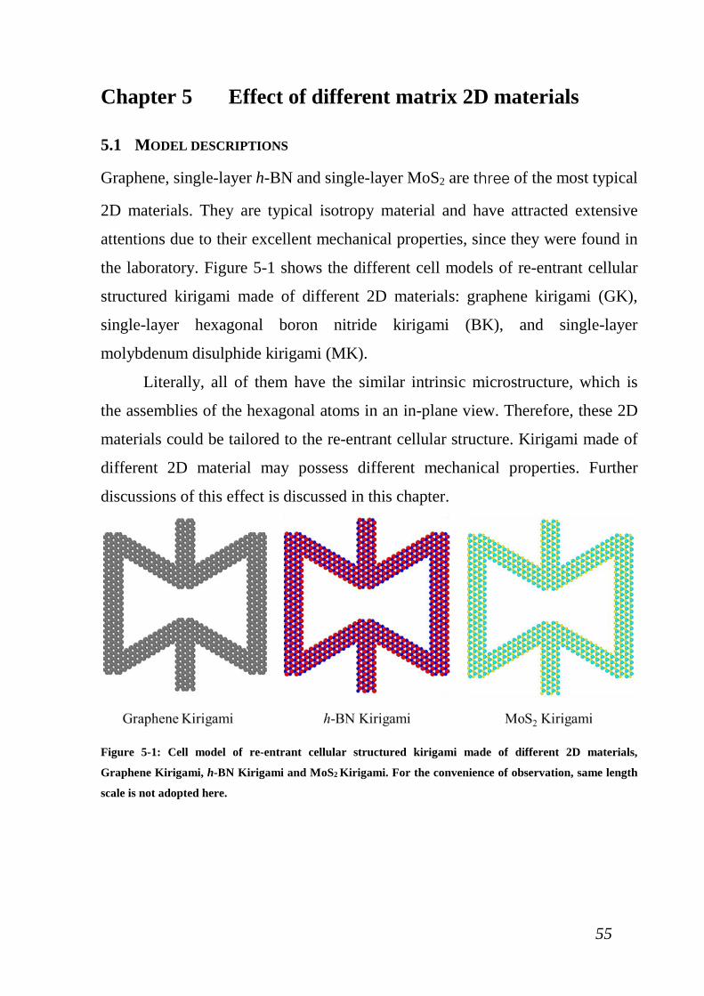
55
Chapter 5 Effect of different matrix 2D materials
5.1 MODEL DESCRIPTIONS
Graphene, single-layer h-BN and single-layer MoS2 are three of the most typical
2D materials. They are typical isotropy material and have attracted extensive
attentions due to their excellent mechanical properties, since they were found in
the laboratory. Figure 5-1 shows the different cell models of re-entrant cellular
structured kirigami made of different 2D materials: graphene kirigami (GK),
single-layer hexagonal boron nitride kirigami (BK), and single-layer
molybdenum disulphide kirigami (MK).
Literally, all of them have the similar intrinsic microstructure, which is
the assemblies of the hexagonal atoms in an in-plane view. Therefore, these 2D
materials could be tailored to the re-entrant cellular structure. Kirigami made of
different 2D material may possess different mechanical properties. Further
discussions of this effect is discussed in this chapter.
Figure 5-1: Cell model of re-entrant cellular structured kirigami made of different 2D materials,
Graphene Kirigami, h-BN Kirigami and MoS2 Kirigami. For the convenience of observation, same length
scale is not adopted here.
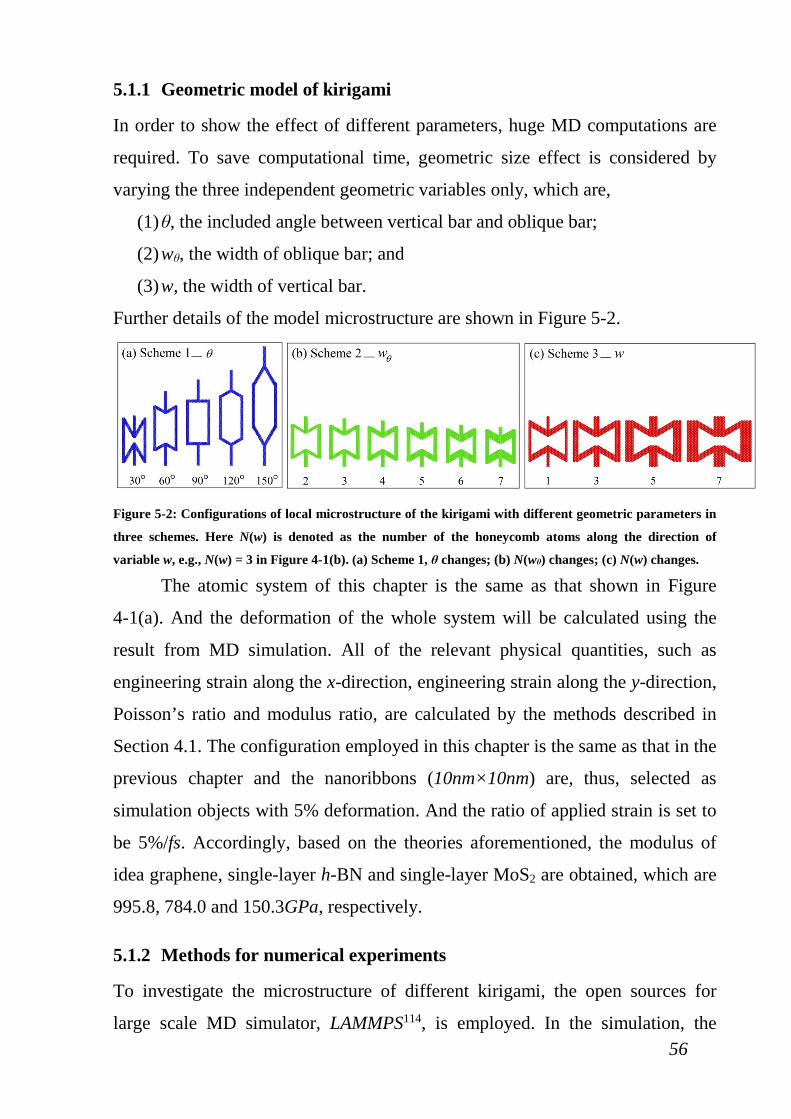
56
5.1.1 Geometric model of kirigami
In order to show the effect of different parameters, huge MD computations are
required. To save computational time, geometric size effect is considered by
varying the three independent geometric variables only, which are,
(1) θ, the included angle between vertical bar and oblique bar;
(2) wθ, the width of oblique bar; and
(3) w, the width of vertical bar.
Further details of the model microstructure are shown in Figure 5-2.
Figure 5-2: Configurations of local microstructure of the kirigami with different geometric parameters in
three schemes. Here N(w) is denoted as the number of the honeycomb atoms along the direction of
variable w, e.g., N(w) = 3 in Figure 4-1(b). (a) Scheme 1, θ changes; (b) N(wθ) changes; (c) N(w) changes.
The atomic system of this chapter is the same as that shown in Figure
4-1(a). And the deformation of the whole system will be calculated using the
result from MD simulation. All of the relevant physical quantities, such as
engineering strain along the x-direction, engineering strain along the y-direction,
Poisson’s ratio and modulus ratio, are calculated by the methods described in
Section 4.1. The configuration employed in this chapter is the same as that in the
previous chapter and the nanoribbons (10nm×10nm) are, thus, selected as
simulation objects with 5% deformation. And the ratio of applied strain is set to
be 5%/fs. Accordingly, based on the theories aforementioned, the modulus of
idea graphene, single-layer h-BN and single-layer MoS2 are obtained, which are
995.8, 784.0 and 150.3GPa, respectively.
5.1.2 Methods for numerical experiments
To investigate the microstructure of different kirigami, the open sources for
large scale MD simulator, LAMMPS114, is employed. In the simulation, the
57
AIREBO potential function96 is used to describe the interaction between the
hydrogen and carbon atoms; the B-N-C Tersoff potential function98 is used to
describe the interaction between the boron and nitrogen atoms; and the SW
potential function102 is used to describe the interaction between molybdenum
and disulphide atoms. The time step used in the simulation is 0.5fs. The
procedure of MD experiment is listed as follows:
(1) Build the kirigami model (within the green frame in Figure 4-1(a)) with
specified geometry;
(2) Maintain the two vertical sides (left and right sides) of the nanostructure
as free boundaries, and the two horizontal sides as periodic boundaries
(Maintain la=lb+lc);
(3) Reshape the structure by minimizing the potential energy of the
nanostructure. The conjugated-gradient algorithm is adopted for updating
the positions of the atoms;
(4) Relax the nanostructure in a Nosé-Hoover thermostat for 200ps with
temperature of 8K;
(5) Provide displacement load along y-direction: the lower side is fixed along
the y-direction and the upper side moves with a strain ratio of 5%/fs. The
total motion costs 1000ps; and
(6) Compute the engineering strains along x- and y-directions according to the
positions of the blue points in Figure 4-1(a). Calculate the Poisson’s ratio
according to equation(5.1). Acquire the equivalent elastic modulus of the
kirigami by using equation(5.2). And the ratio between the equivalent
modulus and that of the ideal graphene, single-layer h-BN and single-
layer MoS2 could emerge easily.
5.2 NUMERICAL RESULTS AND DISCUSSIONS
5.2.1 Results on different angle between vertical and oblique bar
For the first scheme, the internal angle between vertical and oblique bars, θ is
chosen from following angles, i.e., 30, 60, 90, 120 and 150 degrees,
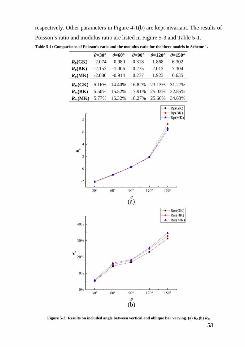
58
respectively. Other parameters in Figure 4-1(b) are kept invariant. The results of
Poisson’s ratio and modulus ratio are listed in Figure 5-3 and Table 5-1. Table 5-1: Comparisons of Poisson’s ratio and the modulus ratio for the three models in Scheme 1.
θ=30° θ=60° θ=90° θ=120° θ=150° Rp(GK) -2.074 -0.980 0.318 1.868 6.302 Rp(BK) -2.153 -1.006 0.275 2.013 7.304 Rp(MK) -2.086 -0.914 0.277 1.923 6.635
Rm(GK) 5.16% 14.40% 16.82% 23.13% 31.27% Rm(BK) 5.50% 15.52% 17.91% 25.03% 32.85% Rm(MK) 5.77% 16.32% 18.27% 25.66% 34.63%
Figure 5-3: Results on included angle between vertical and oblique bar varying. (a) Rp (b) Rm
59
From the results of the Poisson’s ratio for all three kinds of kirigami, it is
fund that the auxetic behaviour could only be observed at the condition of
θ<90°. Besides, in the most of angle conditions of this scheme, all the three
types of kirigami possess the same value of Poisson’s ratio. When oblique bars
perpendicular to vertical bars or in other words, θ=90°, the value of Poisson’s
ratio in three models show positive, instead of zero. Therefore, we can conclude
that main reason that the internal angle affects the auxetic behaviour of this kind
of re-entrant cellular structured kirigami is that rotation of oblique bars.
However, when the angle increases up to 150°, the BK model has the highest
absolute value of Rp, and then, the MK model is in the middle. GK model has
the smallest absolute value of Rp, among the three models.
As for the Modulus ratio in all three types of kirigami, an increase in Rm
could be observed when θ increases. In other words, we could get a higher
modulus when θ becomes higher. The reason could be revealed by the
microstructure of re-entrant cellular structured kirigami. Its deformation results
mainly from the axial linear strain of all the bars when at a higher value of θ.
While, as the θ becomes smaller, rotation of oblique bars would take effects on
the modulus of re-entrant cellular structured kirigami. Accordingly, the structure
with greater θ could obtain larger increment of potential energy. According to
the equation(5.3), it could be concluded that the modulus is larger when θ is
larger. Comparing the value of modulus ratio of different 2D materials, we can
observe that the MK model has the highest value of Rm, the modulus ratio of BK
model is the smallest among three models. With the same geometric
configurations, the re-entrant cellular structured kirigami in MoS2 could get the
largest modulus ratio among three different 2D materials.
5.2.2 Results on different width of oblique bar
In this part, the effect of oblique bars is our major focus. To this end, different
value of N(wθ) is employed (from 2 to 7 is selected). The other parameters in

60
Figure 4-1(b) are kept unchanged. Figure 5-4 and Table 5-2 show the results of
Poisson’s ratio and modulus ratio. Table 5-2: Comparisons of Poisson’s ratio and the modulus ratio for the three models in Scheme 2.
N(wθ)=2 N(wθ)=3 N(wθ)=4 N(wθ)=5 N(wθ)=6 N(wθ)=7 Rp(GK) -0.810 -0.593 -0.470 -0.333 -0.235 -0.178 Rp(BK) -0.835 -0.655 -0.499 -0.371 -0.275 -0.200 Rp(MK) -0.782 -0.555 -0.453 -0.331 -0.237 -0.171
Rm(GK) 3.96% 6.54% 8.21% 9.43% 9.91% 9.92% Rm(BK) 4.12% 6.79% 8.97% 10.38% 11.04% 11.42% Rm(MK) 4.38% 7.39% 9.61% 11.00% 11.68% 11.76%
Figure 5-4: Results on width of oblique bar varying. (a) Rp (b) Rm
61
Firstly, for the Poisson’s ratio, as seen in Figure 5-4 and Table 5-2, the
absolute values of Rp in three models decrease along with an increase in the
width of the oblique bar. The value of Poisson’s ratios ranges from ~-0.8 to ~-
0.2. Besides, due to the internal angle equals to 60°, which is less than 90°, all
the Poisson’s ratios in this scheme are negative. Hence, the auxetic behaviour
could be observed in all the simulations. As for the difference in the three re-
entrant kirigami models, the influence of bulk matrix materials is very obvious.
The kirigami tailored from single-layer h-BN possesses the highest absolute
value of Poisson’s ratio, while the one originated from single-layer MoS2 has the
lowest value.
With regard of the modulus ratio, an obvious increase could be found in
all three models when N(wθ) becomes larger. And the value of Modulus Ratio
ranges from ~4% to ~11%. It could be concluded that the re-entrant
microstructure with wider oblique bars always has a larger value of Rm. As for
the comparison of different modulus ratio for three kinds of 2D materials, the
MK model has the highest value of Rm, the GK model has the lowest value, and
the value of BK model is between the MK model and GK model, which is the
same as the result in scheme 1.
5.2.3 Results on different width of vertical bar
In this scheme, N(w) is chosen to be 1,3,5,7, i.e., the width of vertical bar
increases monotonously, otherwise the other parameters in schematic diagram
are maintained constant. The tendency of Poisson’s ratio and modulus ratio
could be seen in Figure 5-5, and their accurate value are shown in Table 5-3.
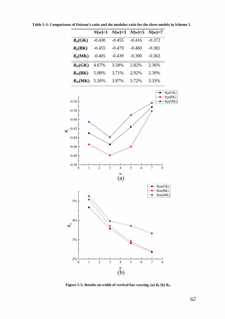
62
Table 5-3: Comparisons of Poisson’s ratio and the modulus ratio for the three models in Scheme 3.
N(w)=1 N(w)=3 N(w)=5 N(w)=7
Rp(GK) -0.430 -0.455 -0.416 -0.372
Rp(BK) -0.455 -0.479 -0.460 -0.381
Rp(MK) -0.405 -0.439 -0.390 -0.363
Rm(GK) 4.67% 3.58% 2.82% 2.36%
Rm(BK) 5.08% 3.71% 2.92% 2.39%
Rm(MK) 5.26% 3.97% 3.72% 3.33%
Figure 5-5: Results on width of vertical bar varying. (a) Rp (b) Rm
63
Unlike the former two schemes, the absolute values of Rp do not vary
monotonously with the variations of width vertical bars. And from the
information in Figure 5-5 and Table 5-3, the absolute value comes to a peak at
N(w)=3. The reason could be revealed by the ratio between width of vertical bar
and length of oblique bar, which is discussed in Subsection 4.2.3. In regards to
the difference among three different 2D materials, the BK model owns the
highest absolute value of Poisson’s ratio, and the absolute value of Poisson’s
ratio in MK is less than that in GK. This kind of variation tendency and
regularity could also be found in scheme 2 and 150° in scheme 1.
As for the modulus ratio among all three models, there is an obvious
decrease in the value of Rm when the vertical bars becomes wider and wider in
the microstructure. The reason could be revealed by the variation of potential
energy of the whole model. As N(w) becoming larger, the decrease of variation
emerges, which results in decreasing of the modulus. In respect to the
comparison of different modulus ratio for three kinds of 2D materials, the MK
model has the highest value of Rm, the GK model has the lowest value. This kind
of tendency and regularity could also be found in the previous two schemes.
5.3 SUMMARY
To conclude, after the analysis of Poisson’s ratios and modulus ratios in three
different kirigami with re-entrant structure, the dependence of the two
mechanical properties on the sizes of microstructure is demonstrated again. And
the mechanical response of different kirigami with geometric similarity is also
calculated for investigating the effect of different matrix 2D materials through
comparisons of the responses.
The results show that the specified Poisson’s ratio and modulus can be
obtained by adjusting the arrangements of microstructure. Some conclusions
could be drawn as following:
(1) From the results of all schemes, when the internal angle between vertical
and oblique bar, θ is less than 90°, all kirigamis show auxetic. On the
contrary, once the internal angle is obtuse, the specific auxetic behaviour
could not happen.
(2) Among all the schemes, in most conditions, the kirigami tailored from
single-layer h-BN owns the highest absolute value of Poisson’s ratio,
while the one originated from single-layer MoS2 has the lowest. As a
result, it can be concluded that, with the similar geometric arrangements
in microstructure, the single-layer h-BN could help the re-entrant cellular
structured kirigami obtain higher absolute Poisson’s ratio value.
(3) From the results shown in all the schemes, the kirigami tailored from
single-layer MoS2 possesses the highest value of modulus ratio, while the
one derived from graphene has the lowest. As a result, it could be
concluded that, with the similar geometric arrangements in
microstructure, the single player MoS2 could make the re-entrant cellular
structured kirigami show stiffer mechanical behaviour.
65
Chapter 6 Conclusions and Future Works
6.1 CONCLUSIONS
In this thesis, an innovative method for achieving nanomaterials with a negative
Poisson’s ratio is demonstrated. After some preliminary investigations on 2D
materials and auxetic materials, we decide to pay more attention on auxetic
behaviour of the re-entrant cellular structured kirigami tailored from 2D
materials.
In general, in order to investigate the size and surface effect on the specific
auxetic behaviour of re-entrant cellular structured kirigami, this work conducts a
systematic study on the different conformational structures. Graphene is selected
as the research subject here. There are five numerical analysis schemes of
different geometric atomic system being adopted to discover the size effect.
Meanwhile, three types of kirigami models including pure GK model,
hydrogenated GK model and macroscopic continuum model, are employed to
explore the surface effect. Some conclusions is obtained as:
(1) Once the internal angle between vertical and oblique bar, θ is less than
90°, the kirigami always show auxetic behaviour.
(2) Of all the conditions, pure carbon GK, being with the highest surface
energy, has the highest absolute value of Poisson’s ratio among the
three models. The absolute value of Poisson’s ratio of the hydrogenated
GK is higher than that of the CK due to the higher surface energy of the
GK than that of the CK.
(3) The modulus ratio of hydrogenated GK is about 10%~20% higher than
that of the pure carbon GK. The modulus ratio of CK is far less than that
of the GK when they have the same geometric configurations. It
demonstrates the surface influence on the modulus of 2D nanomaterials.
In addition, the effect of matrix 2D materials on the performance of re-
entrant cellular structured kirigami is also illustrated in this thesis. There are
66
three kinds of kirigami models being used in this work, including GK model,
BK model and MK model. Some conclusions could be drawn:
(1) Once the internal angel between vertical and oblique bar, θ is less than
90°, the kirigami always show auxetic behaviour.
(2) Among all the models, in most conditions, the kirigami tailored from
single-layer h-BN owns the highest absolute value of Poisson’s ratio,
while the one originated from single-layer MoS2 has the lowest. Thus, it
can be concluded that, with the similar geometric arrangements in
microstructure, the single-layer h-BN could help the re-entrant cellular
structured kirigami obtain higher absolute Poisson’s ratio value.
(3) Of all the models, the kirigami tailored from single-layer MoS2
possesses the highest value of modulus ratio, while the one derived from
graphene has the lowest. As a result, it could be concluded that, with the
similar geometric arrangements in microstructure, the single player
MoS2 could make the re-entrant cellular structured kirigami show
stiffer mechanical behaviour.
6.2 LIMITATIONS
As demonstrated in Section 2.2, auxetic materials have many applications,
however, they also have their own limitations like other materials. Due to the
substantial porosity in these materials, they are normally not stiff enough or not
dense for load-bearing applications. For example, all of the results from Chapter
4 and Chapter 5 show that the maximum modulus ratio is just ~38%, which
proves that the tailoring method makes the re-entrant cellular structured kirigami
is not as stiff as its matrix 2D material.
Besides, MD simulation is not only capable of simulating many
sophisticated systems within modern high-performance research computing
clusters128,129; but also suitable for solving many well-known issues in research
fields. Firstly, the biggest problem of MD simulations is that the length of time
step is small92, which is usually on the order of femtoseconds. Therefore, MD
67
simulations are not capable of simulating experimental time scales of seconds or
even longer95,130. Besides, since the deformation in an MD simulation is
achieved in a very short time frame, the resulting strain ratio is usually nearly 10
orders of magnitude larger than it would be seen in real experiments131,132. In
such a way, an appropriate choice of applied strain ratio is able to describe the
mechanical deformation of materials133–135.
At last, this research work mainly concentrates on the discussions and
analysis on results from numerical simulations. Due to the limitations of
experimental technique nowadays, experimental verification to the most
numerical results obtained in this work is still of problem.
6.3 FUTURE WORKS
As aforementioned, there are some shortcomings in this thesis. Hence, some
improvements are expected to be done in the future to make this research work
more perfect. Next, aiming at the weakness of re-entrant structure solid, which is
not stiff enough, the tension test curve for the kirigami should be further
demonstrated. It usually contains following physical quantities, i.e., the linear
range of plastic strange, the nonlinear range of elastic strain, yield stress, facture
stress and ultimate stress. By studying this clearly and distinctly, some
improvements to modify this weakness could be raised. At last, the new
advanced real experiments to verify the results of this thesis are and always will
be our new research focus in the future.

68
Bibliography
1. Jiang, J.-W., Kim, S. Y. & Park, H. S. Auxetic Nanomaterials: Recent
Progress and Future Development. Appl. Phys. Rev. 3, 41101 (2016).
2. Servantie, J. & Gaspard, P. Rotational dynamics and friction in double-
walled carbon nanotubes. Phys. Rev. Lett. 97, 186106 (2006).
3. Bhimanapati, G. R. et al. Recent Advances in Two-Dimensional Materials
beyond Graphene. ACS Nano 9, 11509–11539 (2015).
4. Kim, S. J., Choi, K., Lee, B., Kim, Y. & Hong, B. H. Materials for
Flexible, Stretchable Electronics: Graphene and 2D Materials. Annu. Rev.
Mater. Res. 45, 63–84 (2015).
5. Novoselov, K. S. et al. Electric Field Effect in Atomically Thin Carbon
Films. Science (80-. ). 306, 666–669 (2004).
6. Nakayama, Y. & Akita, S. Nanoengineering of carbon nanotubes for
nanotools. New J. Phys. 5(1), 128 (2003).
7. Sazonova, V. et al. A tunable carbon nanotube electromechanical
oscillator. Nature 431, 284–7 (2004).
8. Qin, Z., Qin, Q.-H. H. & Feng, X.-Q. Q. Mechanical property of carbon
nanotubes with intramolecular junctions: Molecular dynamics simulations.
Phys. Lett. Sect. A Gen. At. Solid State Phys. 372, 6661–6666 (2008).
9. Cumings, J. & Zettl, A. Low-friction nanoscale linear bearing realized
from multiwall carbon nanotubes. Science (80-. ). 289, 602–604 (2000).
10. Zheng, Q. & Jiang, Q. Multiwalled carbon nanotubes as gigahertz
oscillators. Phys. Rev. Lett. 88, 45503 (2002).
11. Wang, Y., Zhao, Y. J. & Huang, J. P. Giant pumping of single-file water
molecules in a carbon nanotube. J Phys Chem B 115, 13275–13279
(2011).
12. Zhang, S., Liu, W. K. & Ruoff, R. S. Atomistic Simulations of Double-
Walled Carbon Nanotubes (DWCNTs) as Rotational Bearings. Nano Lett.
4, 293–297 (2004).
69
13. Qiu, W., Kang, Y. L., Lei, Z. K., Qin, Q. H. & Li, Q. A New Theoretical
Model of a Carbon Nanotube Strain Sensor. Chinese Phys. Lett. 26, 1–4
(2009).
14. Qiu, W. et al. Experimental study of the Raman strain rosette based on the
carbon nanotube strain sensor. J. Raman Spectrosc. 41, 1216–1220 (2010).
15. Qiu, W., Kang, Y.-L., Lei, Z.-K., Qin, Q.-H. & Li, Q. A new theoretical
model of a carbon nanotube strain sensor. Chinese Phys. Lett. 26, 1–4
(2009).
16. Cai, K., Wan, J., Qin, Q. H. & Shi, J. Quantitative control of a rotary
carbon nanotube motor under temperature stimulus. Nanotechnology 27,
55706 (2016).
17. Cai, K., Yu, J. Z., Yin, H. & Qin, Q. H. Sudden stoppage of rotor in a
thermally driven rotary motor made from double-walled carbon nanotubes.
Nanotechnology 26, 95702 (2015).
18. Cai, K., Cai, H., Yin, H. & Qin, Q. H. Dynamic behavior of curved
double-wall carbon nanotubes with rotating inner tube. RSC Adv. 5,
29908–29913 (2015).
19. Cai, K., Li, Y., Qin, Q. H. & Yin, H. Gradientless temperature-driven
rotating motor from a double-walled carbon nanotube. Nanotechnology 25,
505701 (2014).
20. Cai, K., Yin, H., Qin, Q. H. & Li, Y. Self-excited oscillation of rotating
double-walled carbon nanotubes. Nano Lett 14, 2558–2562 (2014).
21. Evans, K. E. Auxetic polymers: a new range of materials. Endeavour 15,
170–174 (1991).
22. Fung, Y. C. Foundations of solid mechanics. (Prentice Hall, 1965).
23. Beer, F. P., Johnston, E. R. & DeWolf, J. T. Mechanics of Materials.
(2002).
24. Jiang, J.-W. & Park, H. S. Negative Poisson’s Ratio in Single-Layer Black
Phosphorus. Nat. Commun. 5, 4727 (2014).
25. Wang, Y., Li, F., Li, Y. & Chen, Z. Semi-metallic Be5C2 monolayer
70
global minimum with quasi-planar pentacoordinate carbons and negative
Poisson’s ratio. Nat. Commun. 7, 11488 (2016).
26. Milstein, F. & Huang, K. Existence of a negative Poisson ratio in fcc
crystals. Phys. Rev. B 19, 2030–2033 (1979).
27. Ho, D. T., Park, S. D., Kwon, S. Y., Han, T. S. & Kim, S. Y. Negative
Poisson’s ratio in cubic materials along principal directions. Phys. Status
Solidi Basic Res. 253, 1288–1294 (2016).
28. Ashby, M. F. & Medalist, R. F. M. The mechanical properties of cellular
solids. Metall. Trans. A 14, 1755–1769 (1983).
29. Lakes, R. S. Foam Structures with a Negative Poisson’s Ratio. Science
(80-. ). 235, 1038–1040 (1987).
30. Evans, K. E. & Caddock, B. D. Microporous materials with negative
Poisson 鈥s ratios . I . Microstructure and mechanical properties. J 1877–
1882 (1989).
31. Grima, J. N., Mizzi, L., Azzopardi, K. M. & Gatt, R. Auxetic Perforated
Mechanical Metamaterials with Randomly Oriented Cuts. Adv. Mater. 28,
385–389 (2016).
32. Song, F., Zhou, J., Xu, X., Xu, Y. & Bai, Y. Effect of a negative poisson
ratio in the tension of ceramics. Phys. Rev. Lett. 100, 1–4 (2008).
33. Yasuda, H. & Yang, J. Reentrant origami-based metamaterials with
negative Poisson’s ratio and bistability. Phys. Rev. Lett. 114, 185502
(2015).
34. Baughman, R. H. & Galvão, D. S. Crystalline networks with unusual
predicted mechanical and thermal properties. Nature 365, 735–737 (1993).
35. Gere, J. M. Mechanics of Materials. Mechanics of Materials (2008).
doi:10.1016/j.mechmat.2009.01.011
36. Chai, Y., Qin, Q.-H. & Xiao, Y. Recent Patents on Construction Additive
Manufacturing Method. Recent Patents Mech. Eng. 9, 94–101 (2016).
37. Castle, T. et al. Making the cut: Lattice kirigami rules. Phys. Rev. Lett.
113, 245502–245502 (2014).

71
38. Grima, J. N. et al. Tailoring graphene to achieve negative poisson’s ratio
properties. Adv. Mater. 27, 1455–1459 (2015).
39. Shyu, T. C. et al. A kirigami approach to engineering elasticity in
nanocomposites through patterned defects. Nat. Mater. 14, 785–789
(2015).
40. Xu, B. et al. Making negative Poisson’s ratio microstructures by soft
lithography. Adv. Mater. 11, 1186 (1999).
41. Hall, L. J. et al. Sign Change of Poisson’s Ratio for Carbon Nanotube
Sheets. Science 320, 504–507 (2008).
42. Bertoldi, K., Reis, P. M., Willshaw, S. & Mullin, T. Negative poisson’s
ratio behavior induced by an elastic instability. Adv. Mater. 22, 361–366
(2010).
43. Blees, M. K. et al. Graphene kirigami. Nature 524, 204–207 (2015).
44. Jiang, J.-W. & Park, H. S. Negative Poisson’s Ratio in Single-Layer
Graphene Ribbons. Nano Lett. 16, 2657–2662 (2016).
45. Qi, Z., Campbell, D. K. & Park, H. S. Highly Deformable Graphene
Kirigami. 90, 2–6 (2014).
46. Hanakata, P. Z., Qi, Z., Campbell, D. K. & Park, H. S. Highly stretchable
MoS 2 kirigami. Nanoscale 8, 458–463 (2016).
47. Gao, Y., Yang, W. & Xu, B. Unusual thermal conductivity behavior of
serpentine graphene nanoribbons under tensile strain. Carbon N. Y. 96,
513–521 (2016).
48. Wei, N. et al. Thermal conductivity of graphene kirigami: ultralow and
strain robustness. Carbon N. Y. 20, 15–18 (2016).
49. Gupta, A., Sakthivel, T. & Seal, S. Recent development in 2D materials
beyond graphene. Prog. Mater. Sci. 73, 44–126 (2015).
50. Lay, G. Le. 2D materials: Silicene transistors. Nat. Nanotechnol. 10, 202–
203 (2015).
51. Ferrari, A. C. et al. Science and technology roadmap for graphene, related
two-dimensional crystals, and hybrid systems. Nanoscale 7, 4598–4810
72
(2014).
52. Ogino, T. The Nobel Prize in Physics 2010. Hyomen Kagaku 31, 682–682
(2010).
53. Forbes, P. & Grimsey, T. Nanoscience: giants of the infinitesimal.
(Papadakis, 2013).
54. Xu, M., Liang, T., Shi, M. & Chen, H. Graphene-Like Two-Dimensional
Materials. Chem. Rev. 113, 3766–3798 (2013).
55. Zhou, W. et al. Intrinsic structural defects in monolayer molybdenum
disulfide. Nano Lett. 13, 2615–2622 (2013).
56. Lakes, R. Advances in negative Poisson’s ratio materials. Adv. Mater. 5,
293–296 (1993).
57. Milton, G. W. Composite materials with Poisson’s ratios close to -1. J.
Mech. Phys. Solids 40, 1105–1137 (1992).
58. Meisel, M. & Gleick, J. Chaos: Making a New Science. 17 (1988).
59. Grima, J. N. & Evans, K. E. Self expanding molecular networks. Chem.
Commun. 16, 1531–1532 (2000).
60. Grima, J. N., Gatt, R., Alderson, A. & Evans, K. E. On the origin of
auxetic behaviour in the silicate α-cristobalite. J. Mater. Chem. 15, 40–43
(2005).
61. He, C., Liu, P., McMullan, P. J. & Griffin, A. C. Toward molecular
auxetics: Main chain liquid crystalline polymers consisting of laterally
attached para-quaterphenyls. Phys. Status Solidi Basic Res. 242, 576–584
(2005).
62. Lee, J. H., Singer, J. P. & Thomas, E. L. Micro-/nanostructured
mechanical metamaterials. Advanced Materials 24, 4782–4810 (2012).
63. Scarpa, F., Ciffo, L. G. & Yates, J. R. Dynamic properties of high
structural integrity auxetic open cell foam. Smart Mater. Struct. 13, 49–56
(2003).
64. Alderson, A. A triumph of lateral thought. Chem. Ind. 17, 384–391 (1999).
65. Jiang, J.-W. & Park, H. S. Negative Poisson’s Ratio in Single-Layer
73
Graphene Ribbons. Nano Lett. 16, 2657–2662 (2016).
66. Megaw, H. D. Crystal structures: a working approach. (Saunders
Limited., 1973).
67. Amir Yeganeh-Haeri, Donald J. Weidner, J. B. P. Elasticity of alpha-
Cristobalite: A Silicon Dioxide with a Negative Poisson’s Ratio. Science
(80-. ). 257, 650–652 (1992).
68. de Vos Burchart, E., van Bekkum, H., van de Graaf, B. & Vogt, E. T. C. A
consistent molecular mechanics force field for aluminophosphates. J.
Chem. Soc. Faraday Trans. 88, 2761–2769 (1992).
69. Van Beest, B. W. H., Kramer, G. J. & Van Santen, R. A. Force fields for
silicas and aluminophosphates based on ab initio calculations. Phys. Rev.
Lett. 64, 1955–1958 (1990).
70. Casewit, C. J., Colwell, K. S. & Rappe, a. K. Application of a universal
force field to main group compounds. J. Am. Chem. Soc. 114, 10046–
10053 (1992).
71. Diego, S. Cerius2 User Guide. (2000).
72. Grima, J. N., Jackson, R., Alderson, A. & Evans, K. E. Do zeolites have
negative Poisson’s ratios? Adv. Mater. 12, 1912–1918 (2000).
73. Ho, D. T., Park, S.-D., Kwon, S.-Y., Park, K. & Kim, S. Y. Negative
Poisson’s ratios in metal nanoplates. Nat. Commun. 5, 3255 (2014).
74. Baughman, R. H., Shacklette, J. M., Zakhidov, A. A. & Stafstro, S.
Negative Poisson’s ratios as a common feature of cubic metals. Nature
392, 362–365 (1998).
75. Gibson, L. J., Ashby, M. F., Schajer, G. S. & Robertson, C. I. The
Mechanics of Two-Dimensional Cellular Materials. Proc. R. Soc. A Math.
Phys. Eng. Sci. 382, 25–42 (1982).
76. Wang, J.-S., Ye, H.-M., Qin, Q.-H., Xu, J. & Feng, X.-Q. Anisotropic
surface effects on the formation of chiral morphologies of nanomaterials.
in Proc. R. Soc. A rspa20110451 (The Royal Society, 2011).
77. Wang, J.-S., Feng, X.-Q., Xu, J., Qin, Q.-H. & Yu, S.-W. Chirality transfer
74
from molecular to morphological scales in quasi-one-dimensional
nanomaterials: a continuum model. J. Comput. Theor. Nanosci. 8, 1278–
1287 (2011).
78. Spadoni, A. & Ruzzene, M. Elasto-static micropolar behavior of a chiral
auxetic lattice. J. Mech. Phys. Solids 60, 156–171 (2012).
79. Grima, J. N. & Evans, K. E. Auxetic behavior from rotating squares. J.
Mater. Sci. Lett. 19, 1563–1565 (2000).
80. Körner, C. & Liebold-Ribeiro, Y. A systematic approach to identify
cellular auxetic materials. Smart Mater. Struct. 24, 25013 (2015).
81. Novak, N., Vesenjak, M. & Ren, Z. Auxetic cellular materials - a review.
J. Mech. Eng. F, 485–493 (2016).
82. Caddock, B. D. & Evans, K. E. Microporous materials with negative
Poisson’s ratios. I. Microstructure and mechanical properties. J. Phys. D.
Appl. Phys. 22, 1877–1882 (1989).
83. Alderson, K. L. & Evans, K. E. The fabrication of microporous
polyethylene having a negative Poisson’s ratio. Polymer (Guildf). 33,
4435–4438 (1992).
84. Rozvany, G. I. N. Structural design via optimality criteria: the Prager
approach to structural optimization. 8, (Springer Science & Business
Media, 2012).
85. Rana, S. & Fangueiro, R. Advanced Composite Materials for Aerospace
Engineering. (2016).
86. Theocaris, P. S., Stavroulakis, G. E. & Panagiotopoulos, P. D. Negative
Poisson’s ratios in composites with star-shaped inclusions: a numerical
homogenization approach. Arch. Appl. Mech. 67, 274–286 (1997).
87. Liu, Q. Literature review: Materials with negative poisson’s ratios and
potential applications to aerospace and defence. (DTIC Document, 2006).
88. Chan, N. & Evans, K. E. Indentation resilience of conventional and auxetic
foams. J. Cell. Plast. 34, 231–260 (1998).
89. Evans, K. E. & Alderson, A. Auxetic materials: Functional materials and

75
structures from lateral thinking! Adv. Mater. 12, 617–628 (2000).
90. Friis, E. A. Surgical implants incorporating re-entrant material. (1991).
91. Garber, A. M. Pyrolytic materials for thermal protection systems. Aerosp.
Eng. 22, 126–137 (1963).
92. Alder, B. J. & Wainwright, T. E. Studies in Molecular Dynamics. I.
General Method. J. Chem. Phys. 31, 459–466 (1959).
93. J.M.HAILE. Molecular dynamics simulation, elementary methods. J. Mol.
Struct. THEOCHEM. 288, 287–288 (1993).
94. Rapaport, D. C. C. The Art of Molecular Dynamics Simulation. Book 2,
(2004).
95. Frenkel, D. & Berend, S. Understanding Molecular Simulation. (2002).
96. Stuart, S. J., Tutein, A. B. & Harrison, J. A. A reactive potential for
hydrocarbons with intermolecular interactions. J. Chem. Phys. 112, 6472–
6486 (2000).
97. Brenner, D. W. et al. A second-generation reactive empirical bond order
(REBO) potential energy expression for hydrocarbons. J. Phys. Condens.
Matter 14, 783–802 (2002).
98. Tersoff, J. Modeling solid-state chemistry: Interatomic potentials for
multicomponent systems. Phys. Rev. B 39, 5566–5568 (1989).
99. Nord, J., Albe, K., Erhart, P. & Nordlund, K. Modelling of compound
semiconductors: analytical bond-order potential for gallium, nitrogen and
gallium nitride. J. Phys. Condens. Matter 15, 5649–5662 (2003).
100. Tersoff, J. New empirical approach for the structure and energy of
covalent systems. Phys. Rev. B 37, 6991–7000 (1988).
101. Stillinger, F. H. & Weber, T. A. Computer simulation of local order in
condensed phases of silicon. Phys. Rev. B 31, 5262–5271 (1985).
102. Jiang, J.-W. The third principal direction besides armchair and zigzag in
single-layer black phosphorus. Nanotechnology 26, 365702 (2015).
103. Bulatov, V. & Cai, W. Computer simulations of dislocations. 3, (Oxford
University Press on Demand, 2006).
76
104. Abell, G. C. Empirical chemical pseudopotential theory of molecular and
metallic bonding. Phys. Rev. B 31, 6184–6196 (1985).
105. KInacI, A., Haskins, J. B., Sevik, C. & ÇaǧIn, T. Thermal conductivity of
BN-C nanostructures. Phys. Rev. B - Condens. Matter Mater. Phys. 86,
(2012).
106. Jiang, J.-W. Parametrization of Stillinger-Weber potential based on
valence force field model: application to single-layer MoS2 and black
phosphorus. Nanotechnology 26, 315706 (2015).
107. Verlet, L. Computer ‘experiments’ on classical fluids. II. Equilibrium
correlation functions. Phys. Rev. 165, 201–214 (1968).
108. Verlet, L. Computer ‘experiments’ on classical fluids. I. Thermodynamical
properties of Lennard-Jones molecules. Phys. Rev. 159, 98–103 (1967).
109. Gibbs, J. W. Elementary principles in statistical mechanics. (Courier
Corporation, 2014).
110. Ginsburg, T. The conjugate gradient method. Numer. Math. 5, 191–200
(1963).
111. Nosé, S. A unified formulation of the constant temperature molecular
dynamics methods. J. Chem. Phys. 81, 511 (1984).
112. Hoover, W. G. Canonical dynamics: Equilibrium phase-space
distributions. Phys. Rev. A 31, 1695–1697 (1985).
113. Ferguson, A. L. Elements of ICME Research Workshop Molecular
Dynamics with LAMMPS. (2014).
114. Plimpton, S. LAMMPS-large-scale atomic/molecular massively parallel
simulator. Sandia Natl. Lab. (2007).
115. Xia, D. et al. Fabrication of carbon nanoscrolls from monolayer graphene.
Small 6, 2010–2019 (2010).
116. Klimov, N. N. et al. Electromechanical Properties of Graphene
Drumheads. Science (80-. ). 336, 1557–1561 (2012).
117. Lee, C., Wei, X., Kysar, J. W. & Hone, J. Strength of Monolayer Graphene
Measurement of the Elastic Properties and Intrinsic. Science (80-. ). 321,
77
385–388 (2008).
118. Gibson, R. F. Principles of composite material mechanics. (CRC press,
2016).
119. Qi, Z. et al. A molecular simulation analysis of producing monatomic
carbon chains by stretching ultranarrow graphene nanoribbons.
Nanotechnology 21, 265702 (2010).
120. Wang, M. C., Yan, C., Ma, L., Hu, N. & Chen, M. W. Effect of defects on
fracture strength of graphene sheets. Comput. Mater. Sci. 54, 236–239
(2012).
121. Cai, K., Luo, J., Ling, Y., Wan, J. & Qin, Q. Effects of size and surface on
the auxetic behaviour of monolayer graphene kirigami. Nat. Publ. Gr. 1–
10 (2016). doi:10.1038/srep35157
122. Qin, Q. H. Hybrid-Trefftz finite element method for Reissner plates on an
elastic foundation. Comput. Methods Appl. Mech. Eng. 122, 379–392
(1995).
123. Qin, Q.-H. & Wang, H. Matlab and C programming for Trefftz finite
element methods. (CRC Press, 2008).
124. Qin, Q.-H. Variational formulations for TFEM of piezoelectricity. Int. J.
Solids Struct. 40, 6335–6346 (2003).
125. Qin, Q.-H. The Trefftz finite and boundary element method. (Wit
Pr/Computational Mechanics, 2001).
126. Gonze, X. et al. ABINIT: First-principles approach to material and
nanosystem properties. Comput. Phys. Commun. 180, 2582–2615 (2009).
127. Cai, K., Luo, J., Ling, Y., Wan, J. & Qin, Q. Effects of size and surface on
the auxetic behaviour of monolayer graphene kirigami. Sci. Rep. 6, (2016).
128. Abraham, F. F. et al. Simulating materials failure by using up to one
billion atoms and the world’s fastest computer: Work-hardening. Proc.
Natl. Acad. Sci. U. S. A. 99, 5783–5787 (2002).
129. Buehler, M. J., Hartmaier, A., Gao, H., Duchaineau, M. & Abraham, F. F.
Atomic plasticity: Description and analysis of a one-billion atom
78
simulation of ductile materials failure. Comput. Methods Appl. Mech. Eng.
193, 5257–5282 (2004).
130. Allen, M. P. & Tildesley, D. J. Computer simulation of liquids. (Oxford
university press, 1989).
131. Yamakov, V., Wolf, D., Phillpot, S. R., Mukherjee, A. K. & Gleiter, H.
Dislocation processes in the deformation of nanocrystalline aluminium by
molecular-dynamics simulation. Nat. Mater. 1, 45–8 (2002).
132. Wolf, D., Yamakov, V., Phillpot, S. R., Mukherjee, A. & Gleiter, H.
Deformation of nanocrystalline materials by molecular-dynamics
simulation: Relationship to experiments? Acta Materialia 53, 1–40 (2005).
133. Keblinski, P., Wolf, D. & Gleiter, H. Molecular-dynamics simulation of
grain-boundary diffusion creep. Interface Sci. 6, 205–212 (1998).
134. Ikeda, H. et al. Strain Rate Induced Amorphization in Metallic Nanowires.
Phys. Rev. Lett. 82, 2900–2903 (1999).
135. Branício, P. S. & Rino, J. P. Large deformation and amorphization of Ni
nanowires under uniaxial strain: A molecular dynamics study. Phys. Rev.
B - Condens. Matter Mater. Phys. 62, 16950–16955 (2000).

79
Publications
1. Cai, K., Luo, J., Ling, Y., Wan, J. & Qin, Q.H. Effects of size and surface
on the auxetic behaviour of monolayer graphene kirigami. Sci. Rep. 6,
(2016).
2. Luo, J., Cai, K., Qin, Q.H. Auxetic behaviour of re-entrant cellular
structured kirigami tailored from different 2D materials. To be submitted.

80
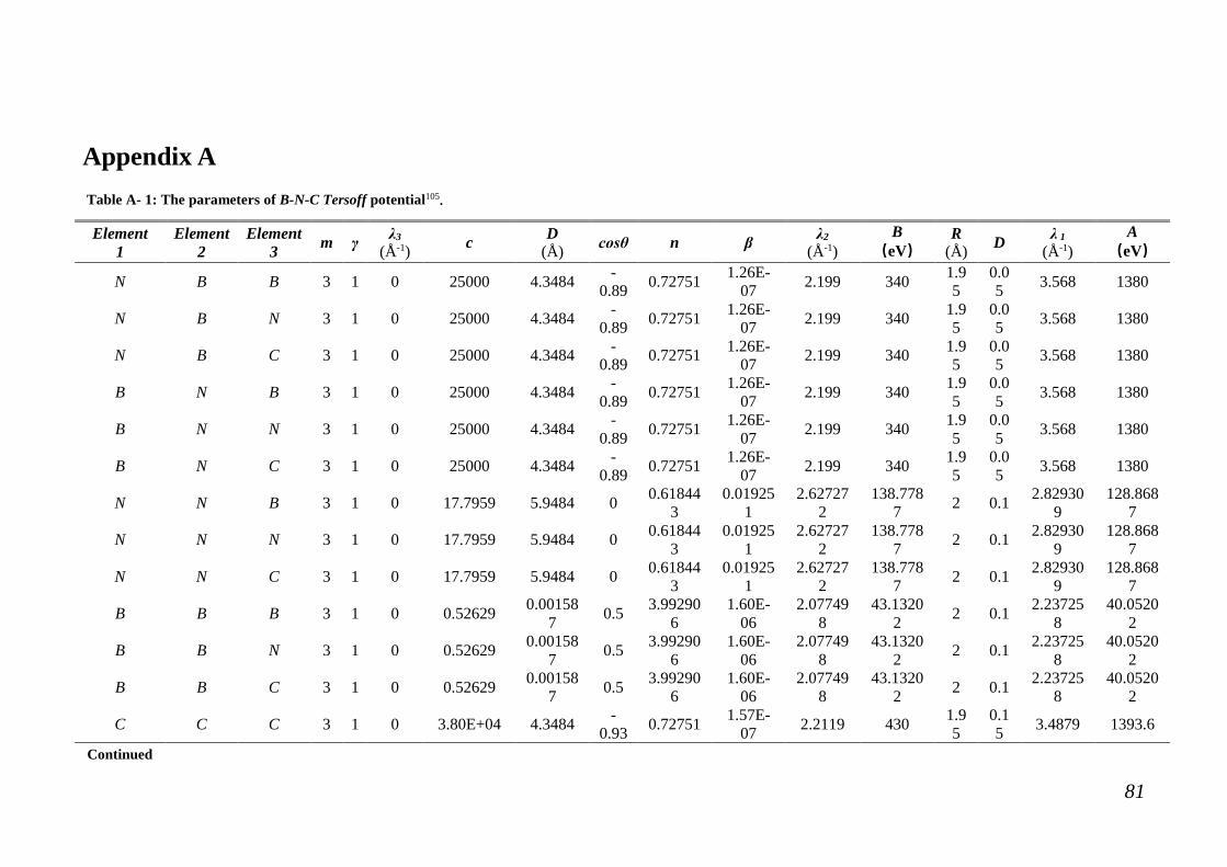
81
Appendix A Table A- 1: The parameters of B-N-C Tersoff potential105.
Element 1
Element2
Element3 m γ λ3
(Å-1) c D (Å) cosθ n β λ2
(Å-1) B
(eV) R
(Å) D λ 1 (Å-1)
A(eV)
N B B 3 1 0 25000 4.3484 -0.89 0.72751 1.26E-
07 2.199 340 1.95
0.05 3.568 1380
N B N 3 1 0 25000 4.3484 -0.89 0.72751 1.26E-
07 2.199 340 1.95
0.05 3.568 1380
N B C 3 1 0 25000 4.3484 -0.89 0.72751 1.26E-
07 2.199 340 1.95
0.05 3.568 1380
B N B 3 1 0 25000 4.3484 -0.89 0.72751 1.26E-
07 2.199 340 1.95
0.05 3.568 1380
B N N 3 1 0 25000 4.3484 -0.89 0.72751 1.26E-
07 2.199 340 1.95
0.05 3.568 1380
B N C 3 1 0 25000 4.3484 -0.89 0.72751 1.26E-
07 2.199 340 1.95
0.05 3.568 1380
N N B 3 1 0 17.7959 5.9484 0 0.618443
0.019251
2.627272
138.7787 2 0.1 2.82930
9 128.868
7
N N N 3 1 0 17.7959 5.9484 0 0.618443
0.019251
2.627272
138.7787 2 0.1 2.82930
9 128.868
7
N N C 3 1 0 17.7959 5.9484 0 0.618443
0.019251
2.627272
138.7787 2 0.1 2.82930
9 128.868
7
B B B 3 1 0 0.52629 0.001587 0.5 3.99290
6 1.60E-
06 2.07749
8 43.1320
2 2 0.1 2.237258
40.05202
B B N 3 1 0 0.52629 0.001587 0.5 3.99290
6 1.60E-
06 2.07749
8 43.1320
2 2 0.1 2.237258
40.05202
B B C 3 1 0 0.52629 0.001587 0.5 3.99290
6 1.60E-
06 2.07749
8 43.1320
2 2 0.1 2.237258
40.05202
C C C 3 1 0 3.80E+04 4.3484 -0.93 0.72751 1.57E-
07 2.2119 430 1.95
0.15 3.4879 1393.6
Continued
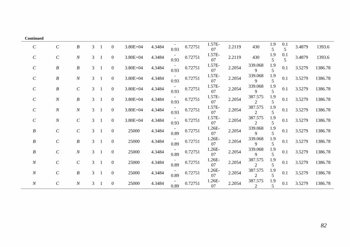
82
Continued
C C B 3 1 0 3.80E+04 4.3484 -0.93 0.72751 1.57E-
07 2.2119 430 1.95
0.15 3.4879 1393.6
C C N 3 1 0 3.80E+04 4.3484 -0.93 0.72751 1.57E-
07 2.2119 430 1.95
0.15 3.4879 1393.6
C B B 3 1 0 3.80E+04 4.3484 -0.93 0.72751 1.57E-
07 2.2054 339.0689
1.95 0.1 3.5279 1386.78
C B N 3 1 0 3.80E+04 4.3484 -0.93 0.72751 1.57E-
07 2.2054 339.0689
1.95 0.1 3.5279 1386.78
C B C 3 1 0 3.80E+04 4.3484 -0.93 0.72751 1.57E-
07 2.2054 339.0689
1.95 0.1 3.5279 1386.78
C N B 3 1 0 3.80E+04 4.3484 -0.93 0.72751 1.57E-
07 2.2054 387.5752
1.95 0.1 3.5279 1386.78
C N N 3 1 0 3.80E+04 4.3484 -0.93 0.72751 1.57E-
07 2.2054 387.5752
1.95 0.1 3.5279 1386.78
C N C 3 1 0 3.80E+04 4.3484 -0.93 0.72751 1.57E-
07 2.2054 387.5752
1.95 0.1 3.5279 1386.78
B C C 3 1 0 25000 4.3484 -0.89 0.72751 1.26E-
07 2.2054 339.0689
1.95 0.1 3.5279 1386.78
B C B 3 1 0 25000 4.3484 -0.89 0.72751 1.26E-
07 2.2054 339.0689
1.95 0.1 3.5279 1386.78
B C N 3 1 0 25000 4.3484 -0.89 0.72751 1.26E-
07 2.2054 339.0689
1.95 0.1 3.5279 1386.78
N C C 3 1 0 25000 4.3484 -0.89 0.72751 1.26E-
07 2.2054 387.5752
1.95 0.1 3.5279 1386.78
N C B 3 1 0 25000 4.3484 -0.89 0.72751 1.26E-
07 2.2054 387.5752
1.95 0.1 3.5279 1386.78
N C N 3 1 0 25000 4.3484 -0.89 0.72751 1.26E-
07 2.2054 387.5752
1.95 0.1 3.5279 1386.78
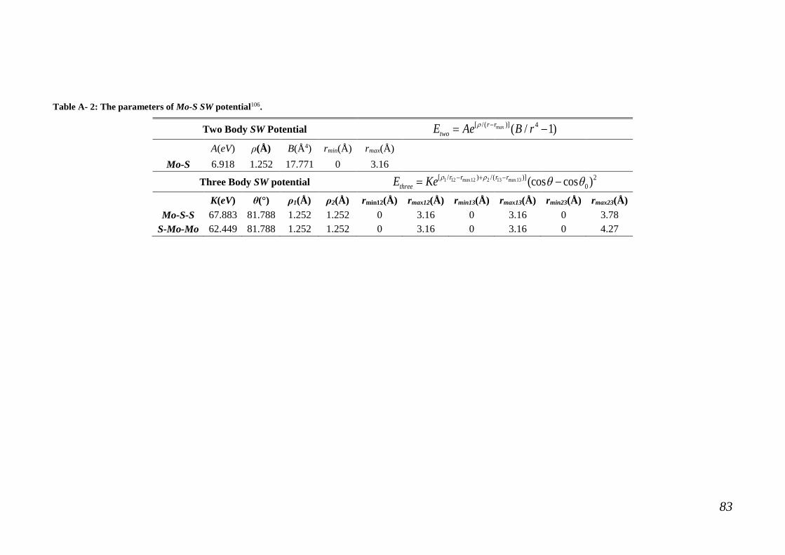
83
Table A- 2: The parameters of Mo-S SW potential106.
Two Body SW Potential max[ /( )] 4( / 1)r rtwoE Ae B rρ −= −
A(eV) ρ(Å) B(Å4) rmin(Å) rmax(Å) Mo-S 6.918 1.252 17.771 0 3.16
Three Body SW potential 1 12 max12 2 13 max13[ / ) /( )] 20(cos cos )r r r r
threeE Ke ρ ρ θ θ− + −= −
K(eV) θ(°) ρ1(Å) ρ2(Å) rmin12(Å) rmax12(Å) rmin13(Å) rmax13(Å) rmin23(Å) rmax23(Å) Mo-S-S 67.883 81.788 1.252 1.252 0 3.16 0 3.16 0 3.78
S-Mo-Mo 62.449 81.788 1.252 1.252 0 3.16 0 3.16 0 4.27
84
Appendix B
MD simulation script for ideal graphene nanoribbon
# ---------- Initialize Simulation ---------------------
clear
dimension 3
units metal
processors 4 4 1
boundary p p p
atom_style full
neighbor 2.0 nsq
neigh_modify every 1 delay 0 check yes
# ---------- Define Interatomic Potential --------------
read_data cellwe.data
pair_style airebo 3.0 1 1
pair_coeff * * CH.airebo C C C C C
# ---------- Create Atom Definition---------------------
group Gbase type 1
group GL1 type 2
group GL2 type 3
group GR1 type 4
group GR2 type 5
variable L1X equal xcm(GL1,x)
variable L1Y equal xcm(GL1,y)
variable L2X equal xcm(GL2,x)
variable L2Y equal xcm(GL2,y)
variable R1X equal xcm(GR1,x)
variable R1Y equal xcm(GR1,y)
85
variable R2X equal xcm(GR2,x)
variable R2Y equal xcm(GR2,y)
variable LX equal "((v_R1X+v_R2X)-(v_L1X+v_L2X))/2"
variable LY equal "((v_L1Y+v_R1Y)-(v_L2Y+v_R2Y))/2"
# ---------- Define Computation Settings ---------------
compute sta all stress/atom NULL
compute PE all pe
variable PE equal c_PE
fix data all ave/time 2000 1 2000 v_L1X v_L1Y v_L2X v_L2Y v_R1X v_R1Y
v_R2X v_R2Y v_LX v_LY v_PE file cellwe.data.txt
# ---------- Energy Minimization ----------------------
timestep 0.0005
dump 1 all custom 1000 relax.cellwe.lammpstrj id mol type x y z fx fy fz
thermo 500
thermo_style custom step temp v_LX v_LY ly
thermo_modify lost ignore
# ---------- Energy Equilibration -------------------
min_style cg
minimize 1.0e-12 1.0e-12 1500 1500
fix fxnpt all npt temp 8.0 8.0 0.1 iso 0.0 0.0 1.0
run 400000
undump 1
unfix fxnpt
write_restart relax.cellwe.restart
# ---------- Set Simulation --------------------
dump 2 all custom 1000 load.cellwe.lammpstrj id mol type x y z fx fy fz
variable Ly equal "ly"
print "Initial Length, Ly=${Ly}"
86
fix fxnvt all nvt temp 8.0 8.0 0.1
variable srate equal 0.05
variable erate equal "v_srate/1.0e3"
fix fxdeform all deform 1 y erate ${erate} units box
run 2000000
write_restart load.cellwe.restart
# ---------- Simulation Done ---------------------------
print "All done"
MD simulation script for de-hydrogenated graphene kirigami
# ---------- Initialize Simulation ---------------------
clear
dimension 3
units metal
processors 4 4 1
boundary p p p
atom_style full
neighbor 2.0 nsq
neigh_modify every 1 delay 0 check yes
# ---------- Define Interatomic Potential --------------
read_data cellw3.data
pair_style airebo 3.0 1 1
pair_coeff * * CH.airebo C C C C C
# ---------- Create Atom Definition---------------------
group Gbase type 1
group GL1 type 2
group GL2 type 3
group GR1 type 4
group GR2 type 5
87
group GC type 1 2 3 4 5
variable L1X equal xcm(GL1,x)
variable L1Y equal xcm(GL1,y)
variable L2X equal xcm(GL2,x)
variable L2Y equal xcm(GL2,y)
variable R1X equal xcm(GR1,x)
variable R1Y equal xcm(GR1,y)
variable R2X equal xcm(GR2,x)
variable R2Y equal xcm(GR2,y)
variable LX equal "((v_R1X+v_R2X)-(v_L1X+v_L2X))/2"
variable LY equal "((v_L1Y+v_R1Y)-(v_L2Y+v_R2Y))/2"
# ---------- Define Computation Settings ---------------
compute sta all stress/atom NULL
compute PE all pe
compute PECa GC pe/atom
compute PEC GC reduce sum c_PECa
fix data all ave/time 2000 1 2000 v_L1X v_L1Y v_L2X v_L2Y v_R1X v_R1Y
v_R2X v_R2Y v_LX v_LY c_PE c_PEC file relax.cellw3.data.txt
# ---------- Energy Minimization ----------------------
timestep 0.0005
dump 1 all custom 1000 relax.cellw3.lammpstrj id mol type x y z fx fy fz
thermo 500
thermo_style custom step temp pe etotal v_LX v_LY ly
thermo_modify lost ignore
# ---------- Energy Equilibration --------------------
min_style cg
minimize 1.0e-12 1.0e-12 1500 1500
88
fix fxnpt all npt temp 8.0 8.0 0.1 iso 0.0 0.0 1.0
run 5000
undump 1
unfix fxnpt
write_restart relax.cellw3.restart
# ---------- Set Simulation --------------------
reset_timestep 0
unfix data
fix data all ave/time 2000 1 2000 v_L1X v_L1Y v_L2X v_L2Y v_R1X v_R1Y
v_R2X v_R2Y v_LX v_LY c_PE c_PEC file load.cellw3.data.txt
dump 2 all custom 1000 load.cellw3.lammpstrj id mol type x y z fx fy fz
variable Ly equal "ly"
print "Initial Length, Ly=${Ly}"
fix fxnvt all nvt temp 8.0 8.0 0.1
variable srate equal 0.05 #5%
variable erate equal "v_srate/1.0e3" #2000000*0.0005=1000ps deform
fix fxdeform all deform 1 y erate ${erate} units box
run 2000000
write_restart load.cellw3.restart
# ---------- Simulation Done ---------------------------
print "All done"
MD simulation script for hydrogenated graphene kirigami
# ---------- Initialize Simulation ---------------------
clear
dimension 3
units metal
processors 4 4 1
boundary p p p
89
atom_style full
neighbor 2.0 nsq
neigh_modify every 1 delay 0 check yes
# ---------- Define Interatomic Potential --------------
read_data cellw3.data
pair_style airebo 3.0 1 1
pair_coeff * * CH.airebo C C C C C H
# ---------- Create Atom Definition---------------------
group Gbase type 1
group GL1 type 2
group GL2 type 3
group GR1 type 4
group GR2 type 5
group GC type 1 2 3 4 5
group GH type 6
variable L1X equal xcm(GL1,x)
variable L1Y equal xcm(GL1,y)
variable L2X equal xcm(GL2,x)
variable L2Y equal xcm(GL2,y)
variable R1X equal xcm(GR1,x)
variable R1Y equal xcm(GR1,y)
variable R2X equal xcm(GR2,x)
variable R2Y equal xcm(GR2,y)
variable LX equal "((v_R1X+v_R2X)-(v_L1X+v_L2X))/2"
variable LY equal "((v_L1Y+v_R1Y)-(v_L2Y+v_R2Y))/2"
# ---------- Define Computation Settings ---------------
compute sta all stress/atom NULL
compute PE all pe
90
compute PECa GC pe/atom
compute PEC GC reduce sum c_PECa
compute PEHa GH pe/atom
compute PEH GH reduce sum c_PEHa
fix data all ave/time 2000 1 2000 v_L1X v_L1Y v_L2X v_L2Y v_R1X v_R1Y
v_R2X v_R2Y v_LX v_LY c_PE c_PEC c_PEH file relax.cellw3.data.txt
# ---------- Energy Minimization ----------------------
timestep 0.0005
dump 1 all custom 1000 relax.cellw3.lammpstrj id mol type x y z fx fy fz
thermo 500
thermo_style custom step temp pe etotal v_LX v_LY ly
thermo_modify lost ignore
# ---------- Energy Equilibration --------------------
min_style cg
minimize 1.0e-12 1.0e-12 1500 1500
fix fxnpt all npt temp 8.0 8.0 0.1 iso 0.0 0.0 1.0
run 400000
undump 1
unfix fxnpt
write_restart relax.cellw3.restart
# ---------- Set Simulation --------------------
reset_timestep 0
unfix data
fix data all ave/time 2000 1 2000 v_L1X v_L1Y v_L2X v_L2Y v_R1X v_R1Y
v_R2X v_R2Y v_LX v_LY c_PE c_PEC c_PEH file load.cellw3.data.txt
dump 2 all custom 1000 load.cellw3.lammpstrj id mol type x y z fx fy fz
variable Ly equal "ly"
print "Initial Length, Ly=${Ly}"

91
fix fxnvt all nvt temp 8.0 8.0 0.1
variable srate equal 0.05
variable erate equal "v_srate/1.0e3"
fix fxdeform all deform 1 y erate ${erate} units box
run 2000000
write_restart load.cellw3.restart
# ---------- Simulation Done ---------------------------
print "All done"
92
Appendix C
MD simulation script for ideal h-BN nanoribbon
# ---------- Initialize Simulation ---------------------
clear
dimension 3
units metal
processors 4 4 1
boundary p p p
atom_style full
neighbor 2.0 nsq
neigh_modify every 1 delay 0 check yes
# ---------- Define Interatomic Potential --------------
read_data SLBN.data
pair_style tersoff
pair_coeff * * BNC.tersoff B N
# ---------- Create Atom Definition---------------------
region GS block 32.5 96.2 18.7 56.4 INF INF
group GS region GS
region GT block 32.5 96.2 56.3 56.4 INF INF
group GT region GT
region GB block 32.5 96.2 18.7 18.8 INF INF
group GB region GB
region GL block 32.5 32.6 18.7 56.4 INF INF
group GL region GL
region GR block 96.1 96.2 18.7 56.4 INF INF
group GR region GR
variable SL equal xcm(GL,x)
93
variable SR equal xcm(GR,x)
variable ST equal xcm(GT,y)
variable SB equal xcm(GB,y)
variable WS equal "v_SR-v_SL"
variable LS equal "v_ST-v_SB"
variable TS equal 3.3306
variable VS equal "v_WS*v_LS*v_TS*1.0e-30"
variable Vall equal "lx*ly*v_TS*1.0e-30"
# ---------- Define Computation Settings ---------------
#all PE
compute PE all pe
#all PES
compute PESa GS pe/atom
compute PES GS reduce sum c_PESa
fix data all ave/time 2000 1 2000 v_LS v_WS v_VS v_Vall c_PE c_PES file
relax.SLBN.data.txt
# ---------- Energy Minimization ----------------------
timestep 0.0005
dump 1 all custom 1000 relax.SLBN.lammpstrj id mol type x y z fx fy fz
thermo 500
thermo_style custom step temp pe ke etotal v_WS v_LS v_VS v_Vall
thermo_modify lost ignore
# ---------- Energy Equilibration --------------------
min_style cg
minimize 1.0e-12 1.0e-12 1500 1500
fix fxnpt all npt temp 8.0 8.0 0.1 iso 0.0 0.0 1.0
run 400000
undump 1
unfix fxnpt
94
write_restart relax.SLBN.restart
# ---------- Set Simulation --------------------
reset_timestep 0
unfix data
fix data all ave/time 2000 1 2000 v_LS v_WS v_VS v_Vall c_PE c_PES file
load.SLBN.data.txt
dump 2 all custom 1000 load.SLBN.lammpstrj id mol type x y z fx fy fz
variable Ly equal "ly"
print "Initial Length, Ly=${Ly}"
fix fxnvt all nvt temp 8.0 8.0 0.1
variable srate equal 0.05
variable erate equal "v_srate/1.0e3"
fix fxdeform all deform 1 y erate ${erate} units box
run 2000000
write_restart load.SLBN.restart
unfix fxdeform
run 600000
# ---------- Simulation Done ---------------------------
print "All done"
MD simulation script for h-BN kirigami
# ---------- Initialize Simulation ---------------------
clear
dimension 3
units metal
processors 4 4 1
boundary p p p
atom_style full
neighbor 2.0 nsq
95
neigh_modify every 1 delay 0 check yes
# ---------- Define Interatomic Potential --------------
read_data BN_w3.data
pair_style tersoff
pair_coeff * * BNC.tersoff B N
# ---------- Create Atom Definition---------------------
group GB type 1
group GN type 2
variable CX1 equal 68.6698
variable CX2 equal 263.8365
variable CY1 equal 68.8598
variable CY2 equal 11.268
variable CR equal 1.45
region GL1 cylinder z ${CX1} ${CY1} ${CR} INF INF units box
region GL2 cylinder z ${CX1} ${CY2} ${CR} INF INF units box
region GR1 cylinder z ${CX2} ${CY1} ${CR} INF INF units box
region GR2 cylinder z ${CX2} ${CY2} ${CR} INF INF units box
group GL1 region GL1
group GL2 region GL2
group GR1 region GR1
group GR2 region GR2
variable L1X equal xcm(GL1,x)
variable L1Y equal xcm(GL1,y)
variable L2X equal xcm(GL2,x)
variable L2Y equal xcm(GL2,y)
variable R1X equal xcm(GR1,x)
variable R1Y equal xcm(GR1,y)
variable R2X equal xcm(GR2,x)
96
variable R2Y equal xcm(GR2,y)
variable LX equal "((v_R1X+v_R2X)-(v_L1X+v_L2X))/2"
variable LY equal "((v_L1Y+v_R1Y)-(v_L2Y+v_R2Y))/2"
# ---------- Define Computation Settings ---------------
#all PE
compute PE all pe
#all PEMo
compute PENa GN pe/atom
compute PEN GN reduce sum c_PENa
#all PES
compute PEBa GB pe/atom
compute PEB GB reduce sum c_PEBa
fix data all ave/time 2000 1 2000 v_L1X v_L1Y v_L2X v_L2Y v_R1X v_R1Y
v_R2X v_R2Y v_LX v_LY c_PE c_PEB c_PEN file relax.BN_w3.data.txt
# ---------- Energy Minimization ----------------------
timestep 0.0005
dump 1 all custom 1000 relax.BN_w3.lammpstrj id mol type x y z fx fy fz
thermo 500
thermo_style custom step temp pe ke etotal v_LX v_LY ly
thermo_modify lost ignore
# ---------- Energy Equilibration --------------------
min_style cg
minimize 1.0e-12 1.0e-12 1500 1500
fix fxnpt all npt temp 8.0 8.0 0.1 iso 0.0 0.0 1.0
run 400000
undump 1
unfix fxnpt

97
write_restart relax.BN_w3.restart
# ---------- Set Simulation --------------------
reset_timestep 0
unfix data
fix data all ave/time 2000 1 2000 v_L1X v_L1Y v_L2X v_L2Y v_R1X v_R1Y
v_R2X v_R2Y v_LX v_LY c_PE c_PEB c_PEN file load.BN_w3.data.txt
dump 2 all custom 1000 load.BN_w3.lammpstrj id mol type x y z fx fy fz
variable Ly equal "ly"
print "Initial Length, Ly=${Ly}"
fix fxnvt all nvt temp 8.0 8.0 0.1
variable srate equal 0.05
variable erate equal "v_srate/1.0e3"
fix fxdeform all deform 1 y erate ${erate} units box
run 2000000
write_restart load.BN_w3.restart
# ---------- Simulation Done ---------------------------
print "All done"
98
Appendix D
MD simulation script for ideal MoS2 nanoribbon
# ---------- Initialize Simulation ---------------------
clear
dimension 3
units metal
processors 4 4 1
boundary p p p
atom_style full
neighbor 2.0 nsq
neigh_modify every 1 delay 0 check yes
# ---------- Define Interatomic Potential --------------
read_data SLMD.data
pair_style sw
pair_coeff * * mos2.sw Mo S
# ---------- Create Atom Definition---------------------
region GS block 41.0 121.4 23.7 71.2 INF INF
group GS region GS
region GT block 41.0 121.4 71.0 71.2 INF INF
group GT region GT
region GB block 41.0 121.4 23.7 23.8 INF INF
group GB region GB
region GL block 41.0 41.1 23.7 71.2 INF INF
group GL region GL
region GR block 121.3 121.4 23.7 71.2 INF INF
group GR region GR

99
variable SL equal xcm(GL,x)
variable SR equal xcm(GR,x)
variable ST equal xcm(GT,y)
variable SB equal xcm(GB,y)
variable WS equal "v_SR-v_SL"
variable LS equal "v_ST-v_SB"
variable VS equal "v_WS*v_LS*6.092*1.0e-30"
variable Vall equal "lx*ly*6.092*1.0e-30"
# ---------- Define Computation Settings ---------------
#all PE
compute PE all pe
#all PES
compute PESa GS pe/atom
compute PES GS reduce sum c_PESa
fix data all ave/time 2000 1 2000 v_LS v_WS v_VS v_Vall c_PE c_PES file
relax.SLMD.data.txt
# ---------- Energy Minimization ----------------------
timestep 0.0005
dump 1 all custom 1000 relax.SLMD.lammpstrj id mol type x y z fx fy fz
thermo 500
thermo_style custom step temp pe ke etotal v_WS v_LS v_VS v_Vall
thermo_modify lost ignore
# ---------- Energy Equilibration --------------------
min_style cg
minimize 1.0e-12 1.0e-12 1500 1500
fix fxnpt all npt temp 8.0 8.0 0.1 iso 0.0 0.0 1.0
run 400000
100
undump 1
unfix fxnpt
write_restart relax.SLMD.restart
# ---------- Set Simulation --------------------
reset_timestep 0
unfix data
fix data all ave/time 2000 1 2000 v_LS v_WS v_VS v_Vall c_PE c_PES file
load.SLMD.data.txt
dump 2 all custom 1000 load.SLMD.lammpstrj id mol type x y z fx fy fz
variable Ly equal "ly"
print "Initial Length, Ly=${Ly}"
fix fxnvt all nvt temp 8.0 8.0 0.1
variable srate equal 0.05
variable erate equal "v_srate/1.0e3"
fix fxdeform all deform 1 y erate ${erate} units box
run 2000000
write_restart load.SLMD.restart
unfix fxdeform
run 600000
# ---------- Simulation Done ---------------------------
print "All done"
MD simulation script for MoS2 kirigami
# ---------- Initialize Simulation ---------------------
clear
dimension 3
units metal
processors 4 4 1
boundary p p p
101
atom_style full
neighbor 2.0 nsq
neigh_modify every 1 delay 0 check yes
# ---------- Define Interatomic Potential --------------
read_data mos2_w3.data
pair_style sw
pair_coeff * * mos2.sw Mo S
# ---------- Create Atom Definition---------------------
group GMo type 1
group GS type 2
fix fixallz GMo setforce NULL NULL 0.0
group Gbase molecule 1
group GL1 molecule 2
group GL2 molecule 3
group GR1 molecule 4
group GR2 molecule 5
variable L1X equal xcm(GL1,x)
variable L1Y equal xcm(GL1,y)
variable L2X equal xcm(GL2,x)
variable L2Y equal xcm(GL2,y)
variable R1X equal xcm(GR1,x)
variable R1Y equal xcm(GR1,y)
variable R2X equal xcm(GR2,x)
variable R2Y equal xcm(GR2,y)
variable LX equal "((v_R1X+v_R2X)-(v_L1X+v_L2X))/2"
variable LY equal "((v_L1Y+v_R1Y)-(v_L2Y+v_R2Y))/2"
# ---------- Define Computation Settings ---------------
#all PE
102
compute PE all pe
#all PEMo
compute PEMoa GMo pe/atom
compute PEMo GMo reduce sum c_PEMoa
#all PES
compute PESa GS pe/atom
compute PES GS reduce sum c_PESa
#fix fixz all setforce NULL NULL 0.0
fix data all ave/time 2000 1 2000 v_L1X v_L1Y v_L2X v_L2Y v_R1X v_R1Y
v_R2X v_R2Y v_LX v_LY c_PE c_PEMo c_PES file relax.mos2_w3.data.txt
# ---------- Energy Minimization ----------------------
timestep 0.0005
dump 1 all custom 1000 relax.mos2_w3.lammpstrj id mol type x y z fx fy fz
thermo 500
thermo_style custom step temp pe ke etotal v_LX v_LY ly
thermo_modify lost ignore
# ---------- Energy Equilibration --------------------
min_style cg
minimize 1.0e-12 1.0e-12 1500 1500
#fix fxnvt all nvt temp 0.1 0.1 0.1
fix fxnpt all npt temp 8.0 8.0 0.1 iso 0.0 0.0 1.0
run 400000
undump 1
unfix fxnpt
write_restart relax.mos2_w3.restart
# ---------- Set Simulation --------------------
reset_timestep 0
unfix data

103
fix data all ave/time 2000 1 2000 v_L1X v_L1Y v_L2X v_L2Y v_R1X v_R1Y
v_R2X v_R2Y v_LX v_LY c_PE c_PEMo c_PES file load.mos2_w3.data.txt
dump 2 all custom 1000 load.mos2_w3.lammpstrj id mol type x y z fx fy fz
variable Ly equal "ly"
print "Initial Length, Ly=${Ly}"
fix fxnvt all nvt temp 8.0 8.0 0.1
variable srate equal 0.05
variable erate equal "v_srate/1.0e3"
fix fxdeform all deform 1 y erate ${erate} units box
run 2000000
write_restart load.mos2_w3.restart
# ---------- Simulation Done ---------------------------
print "All done"