MPIDR WORKING PAPER WP 2011-016SEPTEMBER 2011

Evgeny M. Andreev (andreev@demogr.mpg.de) Ward Kingkade

Average age at death in infancy and infant mortality level: reconsidering the Coale-Demeny formulas at current levels of low mortality

Max-Planck-Institut für demografi sche ForschungMax Planck Institute for Demographic ResearchKonrad-Zuse-Strasse 1 · D-18057 Rostock · GERMANYTel +49 (0) 3 81 20 81 - 0; Fax +49 (0) 3 81 20 81 - 202; http://www.demogr.mpg.de

This working paper has been approved for release by: Vladimir Shkolnikov (shkolnikov@demogr.mpg.de),Head of the Laboratory of Demographic Data.

© Copyright is held by the authors.

Working papers of the Max Planck Institute for Demographic Research receive only limited review.Views or opinions expressed in working papers are attributable to the authors and do not necessarily refl ect those of the Institute.

Average age at death in infancy and infant mortality level: reconsidering the Coale-Demeny formulas at current levels of low mortality

Evgeny M. Andreev* and Ward Kingkade**

Abstract The longterm historical decline in infant mortality has been accompanied by increasing concentration of infant deaths at the earliest stages of infancy. The influence of prenatal and neonatal conditions has become increasingly dominant relative to postnatal conditions as external causes of death such as infectious disease have been diminished. In the mid-1960s Coale and Demeny developed formulas describing the dependency of the average age of death in infancy on the level of infant mortality.

Almost at the same time as Coale and Demeny’s analysis, as shown in this paper, in the more developed countries a steady rise in average age of infant death began. This paper demonstrates this phenomenon with several different data sources, including the linked individual birth and infant death datasets available from the US National Center for Health Statistics and the Human Mortality Database. A possible explanation for the increase in average age of death in infancy is proposed, and modifications of the Coale-Demeny formulas for practical application to contemporary low levels of mortality are offered. Introduction During the period from the 1920s to the 1970s infant mortality decline in Europe and other industrialized countries was accompanied by concentration of infant deaths in the neonatal period. The distribution of infant deaths became more and more highly skew. The average length of life for infants who died during the first year in low-mortality countries was less than 0.25, and exhibited systematic decline as the infant mortality rate (IMR) decreased.

The eminent French demographer Jean Bourgeois-Pichat proposed an explanation of this phenomenon [1951a,b]. He maintained that there are two types of infant mortality: exogenous mortality due to the influence of postnatal conditions as infants become exposed to the external environment, and endogenous mortality due to conditions of the prenatal period, including congenital diseases. Endogenous mortality is concentrated in the first month of life and its level is relatively stable through time. In general, historical mortality decline has been connected with declining exogenous mortality, including in infancy. Thus, rapid infant mortality decline was observed at ages 1-11 months. Bourgeois-Pichat also derived a formula for the distribution of infant deaths by age in infancy as the level of infant mortality varied, together with other determinants of infant mortality.

The average duration until death for infants who die is an important parameter in life table construction. In this connection the Bourgeois-Pichat formula leaves something to be desired. The formula appears rather complicated and demands additional data beyond what is needed to compute the infant mortality rate. For life table construction other purposes, such as calculation of infant mortality rates from infant death rates, simpler formulas (e.g. Chiang, 1978) have been preferred. A set of formulas known as the “Coale-Demeny formulas” that * Max Planck Institute for Demographic Research. Rostock, Germany. ** 1201 Belle View Boulevard, Alexandria, Virginia, 22303. USA. WardKingkade@yahoo.com.

2

describe the relation between the infant mortality rate and the average age of infant death have been the most widely used.

The history of these formulas is as follows. In the early 1960s Ansley J. Coale and Paul Demeny developed for their influential series of the regional model life tables an algorithm for calculating , the average age of death in age interval [0,1) for infants who died in the interval [1966, p. (20)]. This important parameter is necessary for beginning the life table. The number of person-years lived at in the interval from birth to exact age 1, , is related to

, the number of survivors to age 1 and , the hypothetical number of births, by the actuarial relation

01a

01 L

1l 0l

10100101 )1( lalaL ⋅−+⋅= , which leads in turn to the following formula for deriving the infant mortality rate, , from the death rate observed in the age interval from 0 to 1, 1m0: 01 q

0101

0101 )1(1 ma

mq⋅−+

= .

Table 1. Ansley J. Coale and Paul Demeny formulas for estimation of average age of death in infancy based on the infant mortality rate 0q

Regional family of model life tables

For females For males

if infant mortality rate 1 1.00 ≥q

"West," "North," "South" 0.35 0.33

“East” 0.31 0.29

if infant mortality rate 1 1.00 <q

"West," "North," "South" 0.050+3.000 · 01q 0.0425+2.875 · 01q

“East” 0.010+3.000 · 01q 0.0025+2.875 · 01q

Note. Coale and Demeny denoted average age of death in the age interval 0-1 with but we have adopted a parallel notation.

0k

These formulas for were a minor detail within the Coale-Demeny system of model life tables, which has been variously employed to describe relations between levels of fertility and mortality on the one hand, and population structure on the other hand, and which has been widely applied in demographic analysis of Third World countries lacking reliable vital statistics, as well as historical demography of European populations. Somewhat ironically, the formulas for seem to have found more widespread use than the model life table system itself, being employed in the construction of life tables for many analyses which have not otherwise involved the model life tables.

01a

01a

In the 1970s related formulas were developed for calculation average age of infant death based on the central death rate at age 0: [Arriaga, Anderson and Heligman, 1976]. They 01 M

3

used only the higher (for regions "West," "North," "South") variant1 of the formula. These formulas were installed under the name of the “Coale Demeny formula” (C-D formula).

Subsequently, in the 1980s, the “C-D formula” was included in the UN software package for mortality measurement MORTPAK [1988]. In 2001 it was advocated as the basic formula for calculation of the average age of infant death and for calculation of based on [Preston, Heuveline, Guillot, 2001, P. 47]. Finally it became a basic formula employed in the Human Mortality Database (HMD) (Wilmoth et al., 2007) that was launched in May 2002. The C-D formula continues to be recommended for calculation of in textbooks at the present time.

01q 01 M

01a

Mortality declines observed since the 1970s provide evidence that the decline in the average age of infant death ceases when infant mortality rates fall to levels around 0.017-0.022. This calls into question the appropriateness of the Coale-Demeny formula for modern low levels of mortality. To be specific, the C-D formula indicates that if 011.001 <q , the average age of infant death is less than 0.8 month. However in the US life tables for period 2000 and later with [Arias et al., 2010] the average of infant death exceeds 1.3 months. 008.001 <q

The Human Life Table database (HLD), as of February 1, 2011, includes about 4000 life tables. Unfortunately national statistical offices rarely publish all of the standard life table functions. The columns and are frequently absent and it is not possible to estimate what was actually used in a given calculation due to lack of appropriate detail

xLτ xaτ

01a 2. Some countries use the C-D formula or use a fixed value. For example in all official life tables for France is equal to ½. We found in the HLD 277 national level life tables for 23 countries or regions (Australia, Austria, Canada, Chile, Cuba, Germany

01a

01a3, Greece, Hong

Kong, Hungary, Ireland, Italy, Japan, New Zealand, Poland, Portugal, Singapore, Slovenia, Spain, Taiwan, United States of America) with male infant mortality rates less 0.010 and which have been published with all details needed to estimate the exact value of average agof infant death, 01a hese 01a are neither constant for all current national life tables nor they consistent with the C-D formula. According to the C-D form a 01a should be less than one month, but the average ages of infant deaths in the assembled life tables exceed on average what is indicated by the C-D formula by a factor of 3.1 for males and 2.8 for femaleIn all these life tables except those for Italy, the average age of infant death is more than 1 month, sometimes considerably more, when the corresponding estimates by the C-D formula are less than 1 month. In Japan (2007), having the lowest infant mortality level in the database, the difference is 1.9 months; in the USA (2005) it is

e T are

ul

s.

0.7 months.

.

In the analysis below, we attempt to estimate the actual dynamics of the average age of infant death based on vital statistics data for the United States. These data permit us to demonstrate that the decline of average age of infant death synchronous with infant mortality decline becomes interrupted when the infant mortality rate attains a level of about 10 per 1000 newborn infants. Based on the unique datasets of linked individual birth and infant death

1 For each sex separately, there is a single formula for models North, South, and West, while the model East formula differs from the other three models. 2 Actually, can be estimated from , e0 and e1, but usually ex is published with one or two digits after the decimal point, and, consequently, relative error in the estimated average age is very high.

01 L 01q

3 We used data for both the East and the West parts of Germany.

4

records available from the National Center for Health Statistics of the U.S. Centers for Disease Control and Prevention we seek to explain why major infant mortality decline can be combined with relatively high age of infant death.

Data and methods Methods of calculating average age of death in infancy

For precise computation of the average age of infant death it is necessary to have either the aggregate distribution deaths by age in great detail (e.g. days), or, at a minimum, in days during first month of life and weeks for months 2-12; microdata containing this detail would also be adequate, as in the US case. Regrettably, as a result of infant mortality decrease, national statistical offices as well as international organizations have reduced the amount and degree of detail in the infant mortality data they publish. Unlike the1960s and 1970s, in modern publications age in infancy is often provided only in three age groups: 0-6 days, 7-27 days, and 28 or more days.

Fortunately there is an approximation formula for calculation of the average age of death in infancy in an annual birth cohort. This formula uses only numbers of deaths by Lexis triangles. According to this formula, the average age of infant deaths equals the ratio of the number of deaths in the upper Lexis triangle )1,,0( +ttD to the total number of deaths at age 0 in the birth cohort to which these deaths refer:

))1,,0(),,0(()1,,0(01 +++= ttDttDttDa , (1)

where is number of death in age ),,( tyxD x in the cohort of year of birth during calendar year . For birth cohort y in the age interval

yt x to x +1, the triad ( , , 1)x y t + corresponds to the

upper triangle, while represents the lower triangle. The formula is correct under two conditions: 1) the distribution of births throughout the year of birth is uniform; 2) the probabilities of survival to ages less than 1 do not depend on the date of birth within the year.

),,( tyxD

These limitations are typical for demographic calculations. In a sense this formula is equivalent to one of the basic formulas of the cohort component method of population projections: the number of newborn infants survived to the end of the calendar year of birth is

equal 0

01

lLb ⋅ ( stands the total number of newborn infants in the given calendar year);

alternatively, if , then this number is

b

10 =l 01 Lb⋅ (cf. Keyfitz and Flieger, 1971, in which 5 should be modified to 1 because we are dealing with single years in this instance). The total number of cohort survivors to age 1 is 1lb ⋅ . Thus the righthand side of (1) derives from the methodology of population projection: ( ) ( ) ( ) ( )11011101 1 llLlbblbLb −−=⋅−⋅−⋅ . Inserting into the last expression the formula for (in the square brackets) we obtain 01 L

[ ]01

1

101

1

110101

1)1(

1)1(1 a

lla

lllaa

=−−⋅

=−

−⋅−+⋅.

A more thorough derivation of this equation is given in Appendix 1.

The results obtained through this equation (henceforth termed “the triangle-based formula”) are compared to those obtained by direct calculation based on observed dates of birth and death in infancy through record linkage in the analysis below.

5

Decomposition of Changes in average age of death in infancy by cause of death

For investigation of the dynamics of by cause of death, we have used a decomposition method described elsewhere [Andreev, et al., 2002], which is very similar to that advanced by Kitagawa [1955], to estimate the relative contributions of different causes of death to changes in . It is clear that average age of death in infancy can be calculated on the basis of the probability of death from separate causes of death and cause-specific average ages of infant death :

01a

01aiq0

ia0

0100101 qqaai

ii ⎟⎠

⎞⎜⎝

⎛ ⋅= ∑ , (2)

where i indicates a cause of death. If we have data for two periods and then the differences can be decomposed into sums of 1) components

corresponding to changes in cause-specific average ages of infant death ; and 2) components reflecting cause-specific probabilities of death . For this we should write the formula (2) for the second period and perform a chain of systematic replacements or

with the corresponding or . Changes in average age due to each replacement represent an estimate of or . However this estimate depends on the order of the replacements. For this reason, we carry out all possible chains of replacement and calculate the mean contribution of each and across all possible permutations.

),( 0110

11

ii qa),( 0

iq120

12

ia 0110

21 aa −

)( 01iaΔ

)( 01iqΔ

ia021

iq021

ia011

iq011

)( 01iqΔ )( 01

iaΔ

ia01iq01

Data

Our analysis draws upon several datasets, the first being the Human Mortality Database (HMD) available at http://www.mortality.org . The HMD is an online database containing detailed data on period and cohort mortality and survival. Currently it includes 37 countries with reliable mortality statistics. All numbers of deaths in the HMD are presented as numbers of deaths in Lexis triangles. However, for the most part these triangles contain the results of splitting numbers of deaths by year and age of death into Lexis triangles (Wilmoth et al., 2007, p. 11-14) in a manner that in many cases predetermines the dependency of on . The present analysis investigates this relationship and requires data for countries and periods originally received in tabulated form by year of birth, year of death and age at death, or microdata in which these three variables are indicated for each infant death included. However, even in this case numbers of deaths presented in the HMD may still be adjusted, for example as a result of prior redistribution of deaths of unknown age. To avoid possibility of artifacts, we have decided to use the initial (in HMD terms “raw”) numbers of deaths. We have collected all raw numbers of deaths tabulated by Lexis triangle presented at HMD website. (Downloaded February 3, 2011).

01a iq01

Some raw data were excluded from our research because they were corrected previously due to some defects in the initial statistical data. The main problem is “false stillbirths”, a situation where infants that were born alive but died before the birth was registered were reported as stillbirths rather than infant deaths. This has led us to exclude from our dataset observations for France prior to 1975 [Glei et al, 2009] and Netherlands prior to 1950 [Jasilionis, 2009]. Data for Taiwan were excluded due to “systematic under-registration of infant deaths” [Canudas-Romo et al, 2010]. In addition, some East-European countries kept up to the 1960s or later the League of Nations’ definition of live births and stillbirths adopted in 1925,

6

according to which deaths of infants with body mass less than 1000 g. at age less then 7 days were registered as stillbirths: Bulgaria (completely) [Philipov, Jasilionis 2010], the Czech republic (until 1964) [Rychtarikova, Jasilionis, Grigoriev, 2011], East Germany (completely) [Scholz, Jdanov, Kibele, 2011], Estonia (until 1992) [Jasilionis, 2010] , Poland (until 1994) [Fihel, Jasilionis, 2011], the Slovak Republic (until 1964) [Mészáros, Jasilionis, 2011], Ukraine (completely) [Pyrozhkov et al, 2006]. Finally, we exclude data for Iceland, where the number of infant deaths is very small and sometimes 001 =a . In this manner we have assembled the initial numbers of deaths before age 1 in Lexis triangles for 1001 cohorts that were born in the period 1901-2008 in the following 22 countries: Austria (1971 - 2007), Belgium (1941 - 2008), Canada (1950 - 2006), Czech republic (since1964) (1965 - 2007), Germany (1991 - 2007), Denmark (1921 - 2007), Estonia (1992 - 2008), Finland (1917 - 2008), France (1975 - 2008), Hungary (1950 - 2005), Italy (1929 - 2005), Japan (1950 - 2008), Norway (1993 - 2007), New Zealand (1980 - 2007), Poland (1995 - 2008), Portugal (1980 - 2008), Slovak Republic (since 1964) (1965 - 2007), Slovenia (1983 - 2008), Spain (1975 - 2005), Sweden (1901 - 2007), USA. (1959 - 2006).

The second source is the WHO Mortality Database available at http://www.who.int/whosis/mort/download/en/index.html. We used data on the distribution of infant deaths by cause for some of the countries mentioned in order to approximate the probability of dying from leading causes of death.

In addition, our analysis draws upon a compilation of the cohort linked birth-infant death datasets from the US National Center for Health Statistics, available for years 1983-1991, and 1995-2004, at http://www.cdc.gov/nchs/data_access/Vitalstatsonline.htm. These files match each death record derived from the death certificate of an infant with the corresponding birth certificate, where possible. The linked data allow us to determine exact ages at death along with other items of interest, such as detailed cause of death and race of mother.

From the linked birth-infant death data files we calculated the total number of deaths and the average exact age at death in infancy using formula (1) for the period under consideration for the total population of the USA from all causes of death and from 5 selected groups of causes: certain conditions originating in the perinatal period (ICD9 codes B45 or ICD10 codes P00 - P96); congenital malformations, deformations and chromosomal abnormalities (codes B44 or Q00 - Q99); diseases of the respiratory system (B31 or B32 J00 - J99); and sudden infant death syndrome (B466 or R95).

These data should help us to tackle the puzzle as to why the decline of exogenous mortality has been associated with a relatively stable average age of infant death.

In 1999, the US NCHS shifted to the ICD 10 classification of cause of deaths in its annual mortality microdatasets. Prior to the implementation of ICD 10, NCHS conducted a comparison study in which a sample of death records filed in 1996 was coded according to both the ICD 9 and ICD 10 classifications. From the crosstabulation of deaths by cause according to the two respective classifications, “comparability ratios” , each indicating the ratio of deaths in an aggregated cause category coded under the ICD 10 rules to the number of deaths in the same category coded under the ICD 9 rules, were calculated. (Anderson et al., 2001). These cross-classifications can also be used to develop “transition coefficients ” for converting underlying causes of death from ICD 9 categories into ICD 10 equivalents. We have opted not to employ these in our analysis, and have instead aggregated the deaths by detailed cause under the classification in effect in the respective years into a small number of broad groups of causes of death. From a crosstabulation of the parallel ICD9/ICD10-coded data from the comparison study, available on the NCHS website, we have confirmed

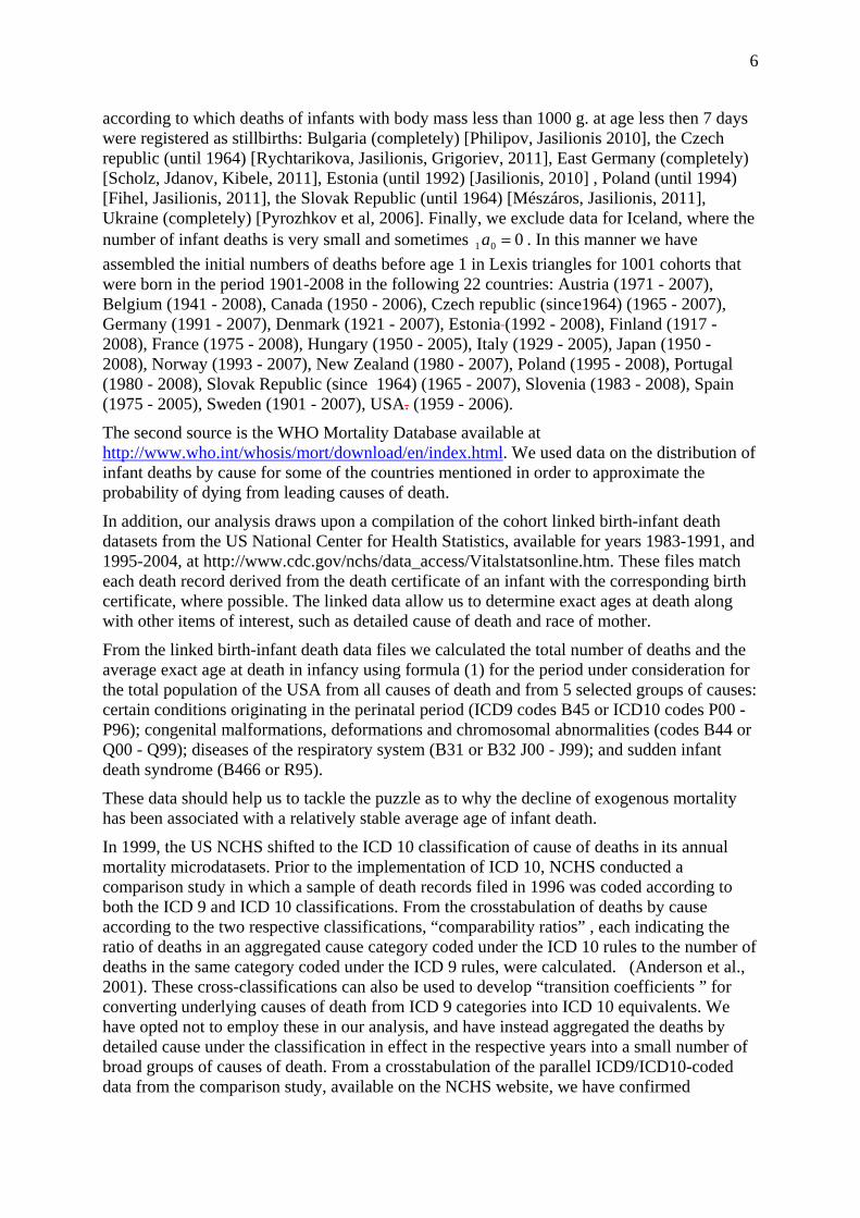
Note: Black points correspond to the beginning and the end of period.

7

0a

01a

Figure 1. Dependence of average age of infant death on the infant mortality rate, by race of mother in birth cohorts 1983-1991, 1995-2004 in the USA .

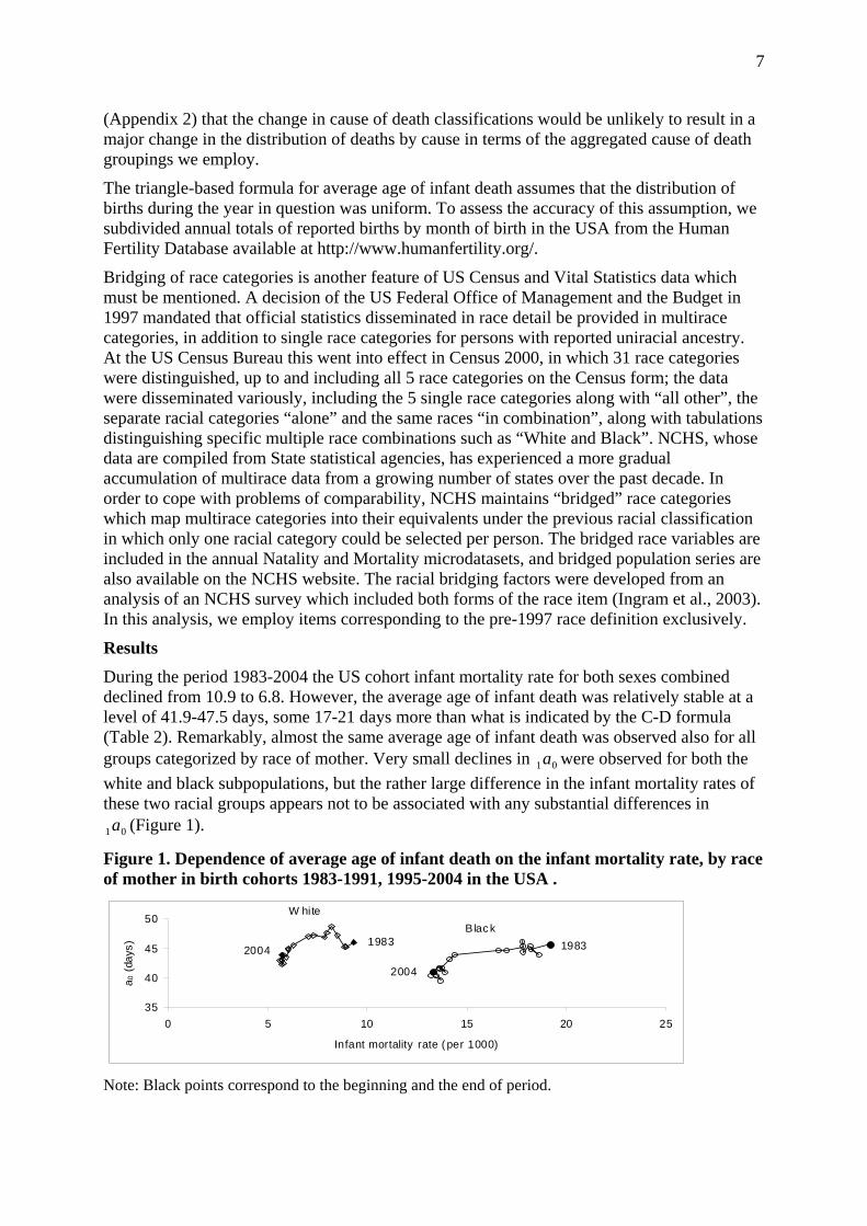
During the period 1983-2004 the US cohort infant mortality rate for both sexes combined declined from 10.9 to 6.8. However, the average age of infant death was relatively stable at a level of 41.9-47.5 days, some 17-21 days more than what is indicated by the C-D formula (Table 2). Remarkably, almost the same average age of infant death was observed also for all groups categorized by race of mother. Very small declines in 1 were observed for both the white and black subpopulations, but the rather large difference in the infant mortality rates of these two racial groups appears not to be associated with any substantial differences in

(Figure 1).

Results

Bridging of race categories is another feature of US Census and Vital Statistics data which must be mentioned. A decision of the US Federal Office of Management and the Budget in 1997 mandated that official statistics disseminated in race detail be provided in multirace categories, in addition to single race categories for persons with reported uniracial ancestry. At the US Census Bureau this went into effect in Census 2000, in which 31 race categories were distinguished, up to and including all 5 race categories on the Census form; the data were disseminated variously, including the 5 single race categories along with “all other”, the separate racial categories “alone” and the same races “in combination”, along with tabulations distinguishing specific multiple race combinations such as “White and Black”. NCHS, whose data are compiled from State statistical agencies, has experienced a more gradual accumulation of multirace data from a growing number of states over the past decade. In order to cope with problems of comparability, NCHS maintains “bridged” race categories which map multirace categories into their equivalents under the previous racial classification in which only one racial category could be selected per person. The bridged race variables are included in the annual Natality and Mortality microdatasets, and bridged population series are also available on the NCHS website. The racial bridging factors were developed from an analysis of an NCHS survey which included both forms of the race item (Ingram et al., 2003). In this analysis, we employ items corresponding to the pre-1997 race definition exclusively.

The triangle-based formula for average age of infant death assumes that the distribution of births during the year in question was uniform. To assess the accuracy of this assumption, we subdivided annual totals of reported births by month of birth in the USA from the Human Fertility Database available at http://www.humanfertility.org/.

(Appendix 2) that the change in cause of death classifications would be unlikely to result in a major change in the distribution of deaths by cause in terms of the aggregated cause of death groupings we employ.

35

40

45

50

0 5 10 15 20 25

Infant mortality rate ( per 1000)

a 0 (

days

)

B lac kW hite

19831983

2004

2004

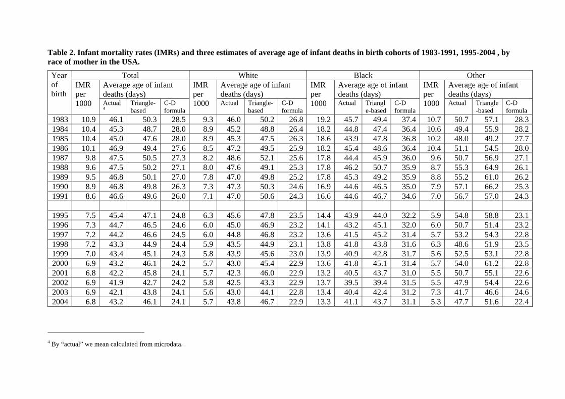
Table 2. Infant mortality rates (IMRs) and three estimates of average age of infant deaths in birth cohorts of 1983-1991, 1995-2004 , by race of mother in the USA.

Total White Black Other Average age of infant deaths (days)

Average age of infant deaths (days)

Average age of infant deaths (days)

Average age of infant deaths (days)

Year of birth

IMR per 1000 Actual

4Triangle-based

C-D formula

IMR per 1000 Actual Triangle-

based C-D formula

IMR per 1000 Actual Triangl

e-based C-D formula

IMR per 1000 Actual Triangle

-based C-D formula

1983 10.9 46.1 50.3 28.5 9.3 46.0 50.2 26.8 19.2 45.7 49.4 37.4 10.7 50.7 57.1 28.3 1984 10.4 45.3 48.7 28.0 8.9 45.2 48.8 26.4 18.2 44.8 47.4 36.4 10.6 49.4 55.9 28.2 1985 10.4 45.0 47.6 28.0 8.9 45.3 47.5 26.3 18.6 43.9 47.8 36.8 10.2 48.0 49.2 27.7 1986 10.1 46.9 49.4 27.6 8.5 47.2 49.5 25.9 18.2 45.4 48.6 36.4 10.4 51.1 54.5 28.0 1987 9.8 47.5 50.5 27.3 8.2 48.6 52.1 25.6 17.8 44.4 45.9 36.0 9.6 50.7 56.9 27.1 1988 9.6 47.5 50.2 27.1 8.0 47.6 49.1 25.3 17.8 46.2 50.7 35.9 8.7 55.3 64.9 26.1 1989 9.5 46.8 50.1 27.0 7.8 47.0 49.8 25.2 17.8 45.3 49.2 35.9 8.8 55.2 61.0 26.2 1990 8.9 46.8 49.8 26.3 7.3 47.3 50.3 24.6 16.9 44.6 46.5 35.0 7.9 57.1 66.2 25.3 1991 8.6 46.6 49.6 26.0 7.1 47.0 50.6 24.3 16.6 44.6 46.7 34.6 7.0 56.7 57.0 24.3 1995 7.5 45.4 47.1 24.8 6.3 45.6 47.8 23.5 14.4 43.9 44.0 32.2 5.9 54.8 58.8 23.1 1996 7.3 44.7 46.5 24.6 6.0 45.0 46.9 23.2 14.1 43.2 45.1 32.0 6.0 50.7 51.4 23.2 1997 7.2 44.2 46.6 24.5 6.0 44.8 46.8 23.2 13.6 41.5 45.2 31.4 5.7 53.2 54.3 22.8 1998 7.2 43.3 44.9 24.4 5.9 43.5 44.9 23.1 13.8 41.8 43.8 31.6 6.3 48.6 51.9 23.5 1999 7.0 43.4 45.1 24.3 5.8 43.9 45.6 23.0 13.9 40.9 42.8 31.7 5.6 52.5 53.1 22.8 2000 6.9 43.2 46.1 24.2 5.7 43.0 45.4 22.9 13.6 41.8 45.1 31.4 5.7 54.0 61.2 22.8 2001 6.8 42.2 45.8 24.1 5.7 42.3 46.0 22.9 13.2 40.5 43.7 31.0 5.5 50.7 55.1 22.6 2002 6.9 41.9 42.7 24.2 5.8 42.5 43.3 22.9 13.7 39.5 39.4 31.5 5.5 47.9 54.4 22.6 2003 6.9 42.1 43.8 24.1 5.6 43.0 44.1 22.8 13.4 40.4 42.4 31.2 7.3 41.7 46.6 24.6 2004 6.8 43.2 46.1 24.1 5.7 43.8 46.7 22.9 13.3 41.1 43.7 31.1 5.3 47.7 51.6 22.4

4 By “actual” we mean calculated from microdata.

9

The results of our calculations by the “triangle-based” approximation formula in all years and for all groups are a little bit higher than the exact values calculated from the microdata. There appears to be a systematic difference averaging 2.5 days for the whole population, as well as for Whites and Blacks separately. This can be explained by departures from the conditions required for accuracy, including, for example, that the distribution of births during the year of birth is not uniform (Figure 2). The number of births during the second half of the each year is on average 6% greater than the number in the first half-year. For this reason, the number of person-years lived in the upper Lexis triangle is on average 1.4% greater than the corresponding number in the lower triangle. This increases the weight of the upper Lexis and leads to overstatement of average age of death in infancy. Note that the differences are almost the same for the whole population, both races, both sexes combined, and for male and female infants separately. However, we consider an error of 2.5 days, or less than 0.7% of a year, to be acceptable.

Figure 2. Average daily number births by month as percent of annual average daily number births in 1983-1991, 1995-2004 in the USA

85

90

95

100

105

110

1 2 3 4 5 6 7 8 9 10 11 12

Month

Perc

ent

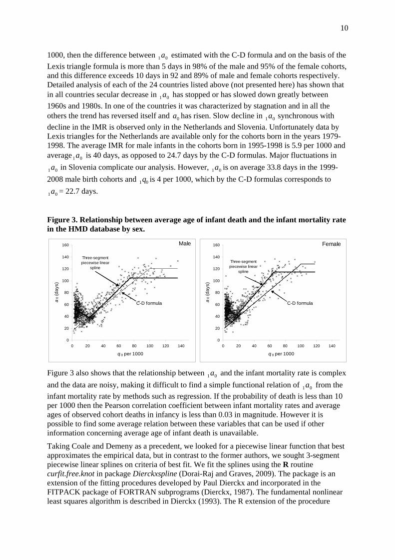
We computed from the HMD input data files by the triangle-based formula and the results of each calculation are plotted as “×” markers in the Figure 3. Simultaneously, we calculated average age of infant death using the C-D formula. The thin black line corresponds to these estimates. The second heavy line in the Figure 3 is our alternative to C-D formula described later.

01a

01a

The estimates from the C-D formula tend to be lower than the triangle-based values for 79% of male cohorts and 90% of female cohorts. If we look only at cohorts with <10 per 1000, then the C-D formulas underestimate for 98% of our observations. In the example for the USA, estimated with the triangle-based formula is on average 2.5 days greater than the actual values calculated from the linked birth and death records. Perhaps analogous circumstances account for the bias in relation to estimates from the C-D formulas. The difference between estimated with the C-D formula and that based on the Lexis triangle formula is more than 5 days in 71% of the male and 80% of the female cohorts. If <10 per

01 q

01a

01a

01a

01 q

10

1000, then the difference between estimated with the C-D formula and on the basis of the Lexis triangle formula is more than 5 days in 98% of the male and 95% of the female cohorts, and this difference exceeds 10 days in 92 and 89% of male and female cohorts respectively. Detailed analysis of each of the 24 countries listed above (not presented here) has shown that in all countries secular decrease in has stopped or has slowed down greatly between 1960s and 1980s. In one of the countries it was characterized by stagnation and in all the others the trend has reversed itself and has risen. Slow decline in synchronous with decline in the IMR is observed only in the Netherlands and Slovenia. Unfortunately data by Lexis triangles for the Netherlands are available only for the cohorts born in the years 1979-1998. The average IMR for male infants in the cohorts born in 1995-1998 is 5.9 per 1000 and average is 40 days, as opposed to 24.7 days by the C-D formulas. Major fluctuations in

in Slovenia complicate our analysis. However, is on average 33.8 days in the 1999-2008 male birth cohorts and is 4 per 1000, which by the C-D formulas corresponds to

= 22.7 days.

01a

01a

0a 01a

01a

01a 01a

01q

01a

Figure 3. Relationship between average age of infant death and the infant mortality rate in the HMD database by sex.

0

20

40

60

80

100

120

140

160

0 20 40 60 80 100 120 140

q 0 per 1000

a0 (

days

)

Male

C-D formula

Three-segment piecewise linear

spline

0

20

40

60

80

100

120

140

160

0 20 40 60 80 100 120 140

q 0 per 1000

a0 (

days

)

Female

C-D formula

Three-segment piecewise linear

spline

Figure 3 also shows that the relationship between and the infant mortality rate is complex and the data are noisy, making it difficult to find a simple functional relation of from the infant mortality rate by methods such as regression. If the probability of death is less than 10 per 1000 then the Pearson correlation coefficient between infant mortality rates and average ages of observed cohort deaths in infancy is less than 0.03 in magnitude. However it is possible to find some average relation between these variables that can be used if other information concerning average age of infant death is unavailable.

01a

01a

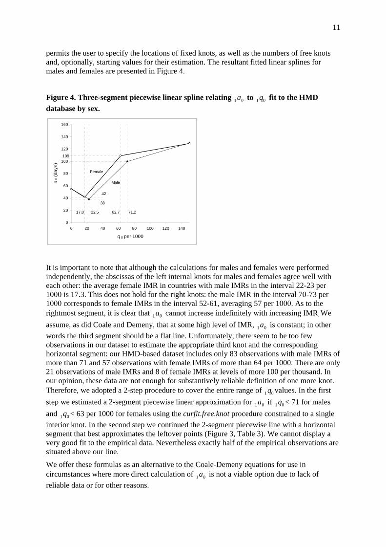
Taking Coale and Demeny as a precedent, we looked for a piecewise linear function that best approximates the empirical data, but in contrast to the former authors, we sought 3-segment piecewise linear splines on criteria of best fit. We fit the splines using the R routine curfit.free.knot in package Dierckxspline (Dorai-Raj and Graves, 2009). The package is an extension of the fitting procedures developed by Paul Dierckx and incorporated in the FITPACK package of FORTRAN subprograms (Dierckx, 1987). The fundamental nonlinear least squares algorithm is described in Dierckx (1993). The R extension of the procedure

11

permits the user to specify the locations of fixed knots, as well as the numbers of free knots and, optionally, starting values for their estimation. The resultant fitted linear splines for males and females are presented in Figure 4.

Figure 4. Three-segment piecewise linear spline relating to fit to the HMD database by sex.

01a 01 q

0

20

40

60

80

100

120

140

160

0 20 40 60 80 100 120 140

q 0 per 1000

a0 (

days

)

Male

Female

22.517.0 71.262.7

38

42

109

It is important to note that although the calculations for males and females were performed independently, the abscissas of the left internal knots for males and females agree well with each other: the average female IMR in countries with male IMRs in the interval 22-23 per 1000 is 17.3. This does not hold for the right knots: the male IMR in the interval 70-73 per 1000 corresponds to female IMRs in the interval 52-61, averaging 57 per 1000. As to the rightmost segment, it is clear that cannot increase indefinitely with increasing IMR. We assume, as did Coale and Demeny, that at some high level of IMR, is constant; in other words the third segment should be a flat line. Unfortunately, there seem to be too few observations in our dataset to estimate the appropriate third knot and the corresponding horizontal segment: our HMD-based dataset includes only 83 observations with male IMRs of more than 71 and 57 observations with female IMRs of more than 64 per 1000. There are only 21 observations of male IMRs and 8 of female IMRs at levels of more 100 per thousand. In our opinion, these data are not enough for substantively reliable definition of one more knot. Therefore, we adopted a 2-step procedure to cover the entire range of values. In the first step we estimated a 2-segment piecewise linear approximation for if < 71 for males and < 63 per 1000 for females using the curfit.free.knot procedure constrained to a single interior knot. In the second step we continued the 2-segment piecewise line with a horizontal segment that best approximates the leftover points (Figure 3, Table 3). We cannot display a very good fit to the empirical data. Nevertheless exactly half of the empirical observations are situated above our line.

01a

01a

01q

01a 01q

01q

We offer these formulas as an alternative to the Coale-Demeny equations for use in circumstances where more direct calculation of is not a viable option due to lack of reliable data or for other reasons.

01a

12

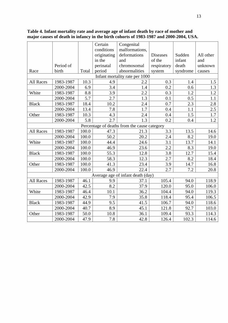
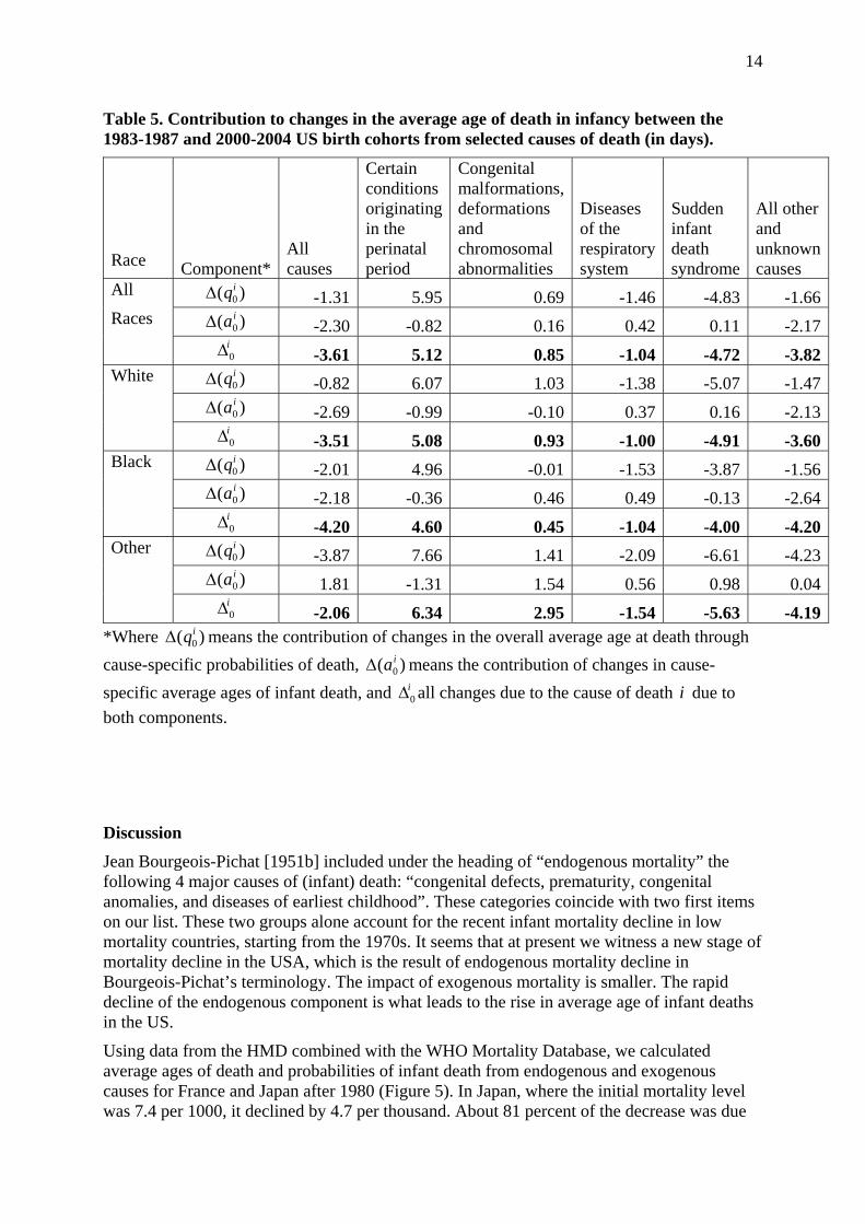
The last results we present pertain to changes in average age of infant death by cause of death. For each race we present result for the first four and last four available cohorts in the US NCHS data, namely the1983-1987 and 2000-2004 birth cohorts (Table 4).

Table 3. Parameters of 3-segment piecewise linear splines recommended for estimation of average age of death in infancy based on the infant mortality rate . 01 q

Lower limits 0q Upper limits 0q Equation Male

0 0.0226 0.1493 - 2.0367· 01 q0.0226 0.0785 0.1035 + 5.5360· 01 q0.0785 + 0.2869

Female 0 0.0170 0.1490 - 2.0867· 01 q

0.0170 0.0658 0.1136 + 6.1942· 01 q0.0658 + 0.3141

Across these periods the infant mortality rate declined from by 6 to 10 points per thousand. The main contributions to this decline (70-76 percent) came from two groups of causes of death: 1) certain conditions originating in the perinatal period and congenital malformations; and 2) deformations and chromosomal abnormalities.

Changes in average age were less significant, but it declined for all race categories by some 2-4 days. Using the decomposition method described above, we can estimate the contribution of each cause to the decline in average age of death in infancy (Table 5).

The results in Table 6 supplement the results in Table 5. The category exercising the strongest impact on changes in infant mortality after 1983 was certain conditions originating in the perinatal period. This group of causes has a positive impact on the infant mortality rate. Because the average age of death from this cause category is very low, mortality decline from these causes exercised an upward influence on the average age of death in infancy.

The very small decline in mortality from sudden infant death syndrome had a somewhat lower influence in the opposite direction. The contribution of mortality from all other and unknown causes to the change in was less important than that due to sudden infant death syndrome but was more important than the contribution of SIDS to the change in average age of death in infancy. Thus, the overall small decrease in average age of infant death is a consequence of offsetting influences. If there was no decrease in mortality from conditions originating in the perinatal period and congenital malformations, then the average age of death in infancy would have decreased by about 7 days.

01q

13

Table 4. Infant mortality rate and average age of infant death by race of mother and major causes of death in infancy in the birth cohorts of 1983-1987 and 2000-2004, USA.

Race Period of birth Total

Certain conditions originating in the perinatal period

Congenital malformations, deformations and chromosomal abnormalities

Diseases of the respiratory system

Sudden infant death syndrome

All other and unknown causes

Infant mortality rate per 1000 All Races 1983-1987 10.3 4.9 2.2 0.3 1.4 1.5 2000-2004 6.9 3.4 1.4 0.2 0.6 1.3White 1983-1987 8.8 3.9 2.2 0.3 1.2 1.2 2000-2004 5.7 2.7 1.3 0.1 0.5 1.1Black 1983-1987 18.4 10.2 2.4 0.7 2.3 2.8 2000-2004 13.4 7.8 1.7 0.4 1.1 2.5Other 1983-1987 10.3 4.3 2.4 0.4 1.5 1.7 2000-2004 5.8 2.7 1.3 0.2 0.4 1.2

Percentage of deaths from the cause category All Races 1983-1987 100.0 47.3 21.3 3.3 13.5 14.6 2000-2004 100.0 50.2 20.2 2.4 8.2 19.0White 1983-1987 100.0 44.4 24.6 3.1 13.7 14.1 2000-2004 100.0 46.9 23.6 2.2 8.3 19.0Black 1983-1987 100.0 55.3 12.8 3.8 12.7 15.4 2000-2004 100.0 58.3 12.3 2.7 8.2 18.4Other 1983-1987 100.0 41.3 23.4 3.9 14.7 16.8 2000-2004 100.0 46.9 22.4 2.7 7.2 20.8

Average age of infant death (day) All Races 1983-1987 46.1 9.9 37.1 105.4 94.0 118.9 2000-2004 42.5 8.2 37.9 120.0 95.0 106.0White 1983-1987 46.4 10.1 36.2 104.4 94.0 119.3 2000-2004 42.9 7.9 35.8 118.4 95.4 106.5Black 1983-1987 44.9 9.5 41.5 106.7 94.0 118.6 2000-2004 40.7 8.9 45.1 121.8 92.7 103.0Other 1983-1987 50.0 10.8 36.1 109.4 93.3 114.3 2000-2004 47.9 7.8 42.8 126.4 102.3 114.6

14

Table 5. Contribution to changes in the average age of death in infancy between the 1983-1987 and 2000-2004 US birth cohorts from selected causes of death (in days).

Race Component* All causes

Certain conditions originating in the perinatal period

Congenital malformations, deformations and chromosomal abnormalities

Diseases of the respiratory system

Sudden infant death syndrome

All other and unknown causes

)( 0iqΔ -1.31 5.95 0.69 -1.46 -4.83 -1.66)( 0

iaΔ -2.30 -0.82 0.16 0.42 0.11 -2.17

All

Races i0Δ -3.61 5.12 0.85 -1.04 -4.72 -3.82

)( 0iqΔ -0.82 6.07 1.03 -1.38 -5.07 -1.47)( 0

iaΔ -2.69 -0.99 -0.10 0.37 0.16 -2.13

White

i0Δ -3.51 5.08 0.93 -1.00 -4.91 -3.60

)( 0iqΔ -2.01 4.96 -0.01 -1.53 -3.87 -1.56)( 0

iaΔ -2.18 -0.36 0.46 0.49 -0.13 -2.64

Black

i0Δ -4.20 4.60 0.45 -1.04 -4.00 -4.20

)( 0iqΔ -3.87 7.66 1.41 -2.09 -6.61 -4.23)( 0

iaΔ 1.81 -1.31 1.54 0.56 0.98 0.04

Other

i0Δ -2.06 6.34 2.95 -1.54 -5.63 -4.19

*Where means the contribution of changes in the overall average age at death through cause-specific probabilities of death, means the contribution of changes in cause-specific average ages of infant death, and all changes due to the cause of death due to both components.

)( 0iqΔ

)( 0iaΔ

i0Δ i

Discussion Jean Bourgeois-Pichat [1951b] included under the heading of “endogenous mortality” the following 4 major causes of (infant) death: “congenital defects, prematurity, congenital anomalies, and diseases of earliest childhood”. These categories coincide with two first items on our list. These two groups alone account for the recent infant mortality decline in low mortality countries, starting from the 1970s. It seems that at present we witness a new stage of mortality decline in the USA, which is the result of endogenous mortality decline in Bourgeois-Pichat’s terminology. The impact of exogenous mortality is smaller. The rapid decline of the endogenous component is what leads to the rise in average age of infant deaths in the US.

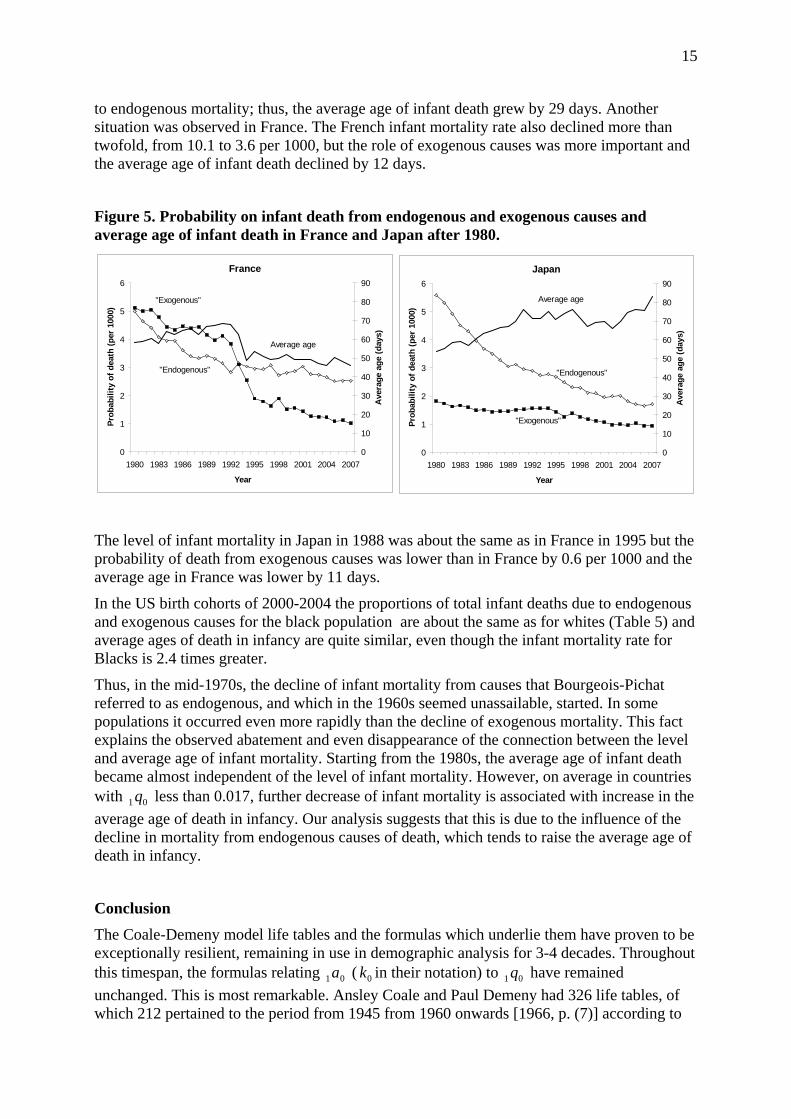
Using data from the HMD combined with the WHO Mortality Database, we calculated average ages of death and probabilities of infant death from endogenous and exogenous causes for France and Japan after 1980 (Figure 5). In Japan, where the initial mortality level was 7.4 per 1000, it declined by 4.7 per thousand. About 81 percent of the decrease was due

15

to endogenous mortality; thus, the average age of infant death grew by 29 days. Another situation was observed in France. The French infant mortality rate also declined more than twofold, from 10.1 to 3.6 per 1000, but the role of exogenous causes was more important and the average age of infant death declined by 12 days.

Figure 5. Probability on infant death from endogenous and exogenous causes and average age of infant death in France and Japan after 1980.

Japan

0

1

2

3

4

5

6

1980 1983 1986 1989 1992 1995 1998 2001 2004 2007

Year

Prob

abili

ty o

f dea

th (p

er 1

000)

0

10

20

30

40

50

60

70

80

90

Ave

rage

age

(day

s)

Average age

"Endogenous"

"Exogenous"

France

0

1

2

3

4

5

6

1980 1983 1986 1989 1992 1995 1998 2001 2004 2007

Year

Prob

abili

ty o

f dea

th (p

er 1

000)

0

10

20

30

40

50

60

70

80

90

Ave

rage

age

(day

s)

Average age

"Endogenous"

"Exogenous"

The level of infant mortality in Japan in 1988 was about the same as in France in 1995 but the probability of death from exogenous causes was lower than in France by 0.6 per 1000 and the average age in France was lower by 11 days.

In the US birth cohorts of 2000-2004 the proportions of total infant deaths due to endogenous and exogenous causes for the black population are about the same as for whites (Table 5) and average ages of death in infancy are quite similar, even though the infant mortality rate for Blacks is 2.4 times greater.

Thus, in the mid-1970s, the decline of infant mortality from causes that Bourgeois-Pichat referred to as endogenous, and which in the 1960s seemed unassailable, started. In some populations it occurred even more rapidly than the decline of exogenous mortality. This fact explains the observed abatement and even disappearance of the connection between the level and average age of infant mortality. Starting from the 1980s, the average age of infant death became almost independent of the level of infant mortality. However, on average in countries with less than 0.017, further decrease of infant mortality is associated with increase in the average age of death in infancy. Our analysis suggests that this is due to the influence of the decline in mortality from endogenous causes of death, which tends to raise the average age of death in infancy.

01 q

Conclusion The Coale-Demeny model life tables and the formulas which underlie them have proven to be exceptionally resilient, remaining in use in demographic analysis for 3-4 decades. Throughout this timespan, the formulas relating ( in their notation) to have remained unchanged. This is most remarkable. Ansley Coale and Paul Demeny had 326 life tables, of which 212 pertained to the period from 1945 from 1960 onwards [1966, p. (7)] according to

01a 0k 01 q

16

Coale and Guang, [1989] data after 1960 practically were not presented in their collection. In this time period the minimum infant mortality rate for both sexes was more than 12 per 1000. It would be miraculous if the empirical formulas based on this dataset remained accurate up to the present moment.

Our assembled data demonstrate that the Coale-Demeny formulas for estimation of the average age of infant death no longer hold for countries with low infant mortality by current standards. In most of these countries, starting from some moment in the process of infant mortality decline, the decrease in the average age of death in infancy has given way to increase. However, the relation between these two indicators is characterized by a reversal in the main effect as well as considerable uncertainty, making it difficult to describe with a “traditional” parametric mathematical model. Our two-knot spline is preferable for mortality modeling.

Inaccuracy in average age estimation does not influence either the magnitude of infant mortality rates or life expectancy. But this average age of death in infancy is an important characteristic of infant mortality and is used in demographic calculations such as life table construction. We recommend calculating the infant mortality rate directly whenever possible, and estimating it by the triangle based formula when not. If estimates of are needed and no other data are available than infant mortality rates by sex, our formulas may be employed. Our analysis shows that these approaches are preferable to the Coale-Demeny formulas at low levels of mortality.

01a

Acknowledgements We are grateful to Dr. Vladimir Shkolnikov from the Max Planck Institute for Demographic Research for useful discussions on some methodological problems and preliminary results.

References Anderson, R.N., A.M. Mininio, D.L. Hoyert, and H.M. Rosenberg. Comparability of Cause of

Death Between ICD-9 and ICD-10: Preliminary Estimates. , National Vital Statistics Reports Vol. 49, No. 2, National Center for Health Statistics.

Andreev EM, Shkolnikov VM, Begun AZ. Algorithm for decomposition of differences between aggregate demographic measures and its application to life expectancies, healthy life expectancies, parity-progression ratios and total fertility rates. Demographic Research 2002;7:499-522

Arias, Elizabeth, Brian L. Rostron, and Betzaida Tejada-Vera (2010) United States Life Tables, 2005. National Vital Statistics Reports, Vol. 58, No. 10

Arriaga Eduardo, Patricia Anderson, Larry Heligman (1976) Computer programs for demographic analysis. United States. Bureau of the Census. Washington.

Bourgeois-Pichat Jean, 1951b, La mesure de la mortalité infantile : II. Les causes de décès, Population, 6 (3), pp. 459-480.

Bourgeois-Pichat, Jean. 1951a. La mesure de la mortalité infantile. Principes et méthodes. Population, 2: 233-248

Canudas-Romo, Vladimir, Danzhen You, Yun-Hsiang Hsu, and Tsung-Hsueh Lu (2010) About mortality data for Taiwan. The Human Mortality Database. Background and documentation.

Chiang, C.L., Life Table and Mortality Analysis. Geneva: World Health Organization. 1978.

17

Coale, Ansley and Guo Guang (1989) Revised regional model life tables at very low levels of mortality Population Index. Vol. 55, No. 4. P. 613-643

Coale, Ansley J., and Paul Demeny (1966). Regional Model Life Tables and Stable Populations. New York: Academic Press.

Dierckx, P., Curve and Surface Fitting with Splines. New York: Oxford University Press. 1993.

Dierckx, P, FITPACK user guide Part 1: curve fitting routines, TW report 89, Department of Computer Science, Katholieke Universiteit. Leuven, Belgium. 1987.

Doray-Raj, S. and S. Graves, Dierckx Spline: R Companion to “Curve and Surface Fitting with Splines”. R package version 1.1-4. http://CRAN.R-project.org/package=DierckxSpline

Fihel, Agnieszka and Domantas Jasilionis (2011) About mortality data for Poland. The Human Mortality Database. Background and documentation. Available at http://www.mortality.org/hmd/POL/InputDB/POLcom.pdf

Glei Dana, France Meslé, Jacques Vallin, John Wilmoth, and Magali Barbieris (2009) About mortality data for France, total population. The Human Mortality Database. Background and documentation. Available at http://www.mortality.org/hmd/FRA/InputDB/FRAcom.pdf

Human Fertility Database (2011). Max Planck Institute for Demographic Research (MPIDR) in Rostock, Germany and the Vienna Institute of Demography (VID) of the Austrian Academy of Sciences, Austria. Available at http://www.humanfertility.org/

Human Life-Table Database (2011). Max Planck Institute for Demographic Research (MPIDR) in Rostock, Germany, the Department of Demography at the University of California at Berkeley, USA, and Institut national d'études démographiques (INED) in Paris, France. Available at http://www.lifetable.de/

Human Mortality Database. (2011). University of California, Berkeley (USA), and Max Planck Institute for Demographic Research (Germany). Available online at http://www.mortality.org/.

Ingram, DD, Parker, JD, Schenker, N, Weed, JA, Hamilton, B, Arrias, E, and Madans, JH, United States Census 2000 population with bridged race categories. National Center for Health Statistics, 2003.

Jasilionis Domantas (2009) About mortality data for the Netherlands. The Human Mortality Database. Background and documentation. Available at http://www.mortality.org/hmd/NLD/InputDB/NLDcom.pdf

Jasilionis Domantas (2010). About mortality data for the Estonia. The Human Mortality Database. Background and documentation. Available at http://www.mortality.org/hmd/EST/InputDB/ESTcom.pdf

Keyfitz, N. and W. Flieger, Population: facts and methods of Demography, W.H. Freeman, 1971.

Kitagawa Evelyn M. (1955) Components of a Difference between Two Rates. Journal of the American Statistical Association, Vol. 50, No. 272, 1168-1194.

18

Mészáros Ján and Domantas Jasilionis (2011) About mortality data for the Slovak Republic. The Human Mortality Database. Background and documentation. Available at http://www.mortality.org/hmd/SVK/InputDB/SVKcom.pdf

MORTPAK (1988): The United Nations Software Package for Mortality Measurement. Batch-oriented Software for the Main frame Computer (ST/ESA/SER.R/78). 264 pp. Non-sales publication (1988).

Philipov, Dimiter and Domantas Jasilionis (2010) About mortality data for Bulgaria. The Human Mortality Database. Background and documentation. Available at http://www.mortality.org/hmd/BGR/InputDB/BGRcom.pdf

Preston, Samuel H., Patrick Heuveline, and Michel Guillot. (2001) Demography: Measuring and Modeling Population Processes. Malden, Massachusetts, United States: Blackwell Publishing.. P. 47.

Pyrozhkov S., N. Foygt, and D.Jdanov (2006) About mortality data for Ukraine. The Human Mortality Database. Background and documentation. Available at http://www.mortality.org/hmd/UKR/InputDB/UKRcom.pdf

R Development Core Team (2011). R: A language and environment for statistical computing. R Foundation for Statistical Computing, Vienna, Austria. ISBN 3-900051-07-0, Available online at http://www.R-project.org/.

Rychtarikova, Jitka, Domantas Jasilionis, Pavel Grigoriev (2011) About mortality data for the Czech Republic. The Human Mortality Database. Background and documentation. Available at http://www.mortality.org/hmd/CZE/InputDB/CZEcom.pdf

Scholz, Rembrandt, Dmitri Jdanov, Eva Kibele (2011) About mortality data for East Germany. The Human Mortality Database. Background and documentation. Available at http://www.mortality.org/hmd/DEUTE/InputDB/DEUTEcom.pdf

WHO Mortality Data base (2010) World Health Organization. Department of Health Statistics and Informatics. Available at http://www.who.int/whosis/mort/download/en/index.html

Wilmoth J.R., K. Andreev, D. Jdanov, and D.A. Glei with the assistance of C. Boe, M. Bubenheim, D. Philipov, V. Shkolnikov, P. Vachon (2007). Methods Protocol for the Human Mortality Database. Last Revised: May 31, 2007 (Version 5). Available at http://www.mortality.org/Public/Docs/MethodsProtocol.pdf

19

Appendix 1. Proof triangle-based formula for average age of deaths.

Consider an annual birth cohort born within year 0 0[ , 1)Y t t= + that satisfies the following two conditions:

- the distribution of births is uniform within Y , (the density function of the birth distribution, )(tβ , is constant within Y );

- the cohort survival function , ),( txl )1,[ 00 +∈ ttt does not depend on date of birth within the age interval . )1,[ 00 +xx

Then the average number of years lived within the age interval )1,[ 00 +xx among people dying at that age is equal to the share of number of deaths in the upper Lexis triangle in the total number of death at age .

)( 0xa

0x

Proof. Let denote the initial size of the birth cohort, and let stand for the cohort survival function. It is obvious that and for

Yb Yxl

Ybt =)(β Yxltxl =),( )1,[ 00 +∈ ttt . It follows that

the number of cohort members attaining age by the end of calendar year t0 is equal

to , where represents the cumulated survivorship function

corresponding to in the age interval to +1. In general, this number of people

is . Taking into account the properties of the cohort assumed

above, this number of people is equal to

0x

Yx

Y Lb01⋅ ∫ +=

1

001 )(

0θθ dxlL YY

x

Yxl 0x 0x

∫ ++−⋅+1

000 ),1()( θθθθβ dtxlt o

.)()1(01

1

00

1

00

Yx

YYYYY Lbdxlbdxlb ⋅=+⋅=+− ∫∫ ξξθθ

Let the parallelogram ABCD (Figure 1-1) correspond to the cohort and age interval under consideration. We should prove that the number of deaths in the triangle BCD divided by the total number of deaths in the parallelogram ABCD is . Y

xa01

Figure 1-1. Lexis parallelogram of deaths in a birth cohort.

20

The number of survivors at age is equal to (the segment AB) and at age is

equal to (the segment DC). The segment BD corresponds to the number of survivors to the end of calendar years

0x Yx

Y lb0

⋅ 10 +x

)1( 0 +⋅ xlb YY

0xY + .and is equal to . Thus the number of

deaths in the upper triangle, BCD, is . If we replace with the formula for

its calculation we find that the number of deaths in the upper

triangle is . The product is exactly number of death in

parallelogram ABCD. So, the ratio of BCD to ABCD is

Vx

Y Lb01⋅

)( 11 00

Vx

Vx

Y lLb +−⋅ VxL

01

))( 1111 00000

Yx

Yx

Yx

Yx

Yx llalL ++ −⋅+=

)( 11 000

Yx

Yx

YYx llba +−⋅⋅ )( 100

Yx

Yx

Y llb +−⋅

YxY

xYx

Y

Yx

Yx

YYx a

llbllba

0

00

0001

1

11

)()(=

−⋅−⋅⋅

+

+

QED

21

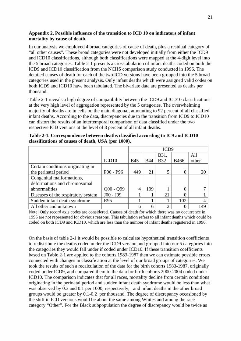
Appendix 2. Possible influence of the transition to ICD 10 on indicators of infant mortality by cause of death. In our analysis we employed 4 broad categories of cause of death, plus a residual category of “all other causes”. These broad categories were not developed initially from either the ICD9 and ICD10 classifications, although both classifications were mapped at the 4-digit level into the 5 broad categories. Table 2-1 presents a crosstabulation of infant deaths coded on both the ICD9 and ICD10 classification from the NCHS comparison study conducted in 1996. The detailed causes of death for each of the two ICD versions have been grouped into the 5 broad categories used in the present analysis. Only infant deaths which were assigned valid codes on both ICD9 and ICD10 have been tabulated. The bivariate data are presented as deaths per thousand.

Table 2-1 reveals a high degree of compatibility between the ICD9 and ICD10 classifications at the very high level of aggregation represented by the 5 categories. The overwhelming majority of deaths are in cells on the main diagonal, amounting to 92 percent of all classified infant deaths. According to the data, discrepancies due to the transition from ICD9 to ICD10 can distort the results of an intertemporal comparison of data classified under the two respective ICD versions at the level of 8 percent of all infant deaths.

Table 2-1. Correspondence between deaths classified according to IC9 and ICD10 classifications of causes of death, USA (per 1000).

ICD9

ICD10 B45 B44B31, B32 B466

All other

Certain conditions originating in the perinatal period P00 - P96 449 21 5 0 20Congenital malformations, deformations and chromosomal abnormalities Q00 - Q99 4 199 1 0 7Diseases of the respiratory system J00 - J99 1 1 21 0 1Sudden infant death syndrome R95 1 1 1 102 4All other and unknown 6 6 2 0 149

Note: Only record axis codes are considered. Causes of death for which there was no occurrence in 1996 are not represented for obvious reasons. This tabulation refers to all infant deaths which could be coded on both ICD9 and ICD10, which are less than the number of infant deaths registered in 1996.

On the basis of table 2-1 it would be possible to calculate hypothetical transition coefficients to redistribute the deaths coded under the ICD9 version and grouped into our 5 categories into the categories they would fall under if coded under ICD10. If these transition coefficients based on Table 2-1 are applied to the cohorts 1983-1987 then we can estimate possible errors connected with changes in classification at the level of our broad groups of categories. We took the results of such a recalculation of the data for the birth cohorts 1983-1987, originally coded under ICD9, and compared them to the data for birth cohorts 2000-2004 coded under ICD10. The comparison indicates that for all races, mortality decline from certain conditions originating in the perinatal period and sudden infant death syndrome would be less than what was observed by 0.3 and 0.1 per 1000, respectively, and infant deaths in the other broad groups would be greater by 0.1-0.2 per thousand. The degree of discrepancy occasioned by the shift in ICD versions would be about the same among Whites and among the race category “Other”. For the Black subpopulation the degree of discrepancy would be twice as

22

much. For instance, mortality decline from certain conditions originating in the perinatal period would be 0.7 per thousand greater than what is indicated in Table 5. However all cause specific death probabilities for the Black subpopulation are about two times greater than the average for all races combined. This is evidence that the change in ICD versions would not alter our conclusions concerning the roles of the broad cause of death categories in the dynamics of average age of infant death.