Economic Research Southern Africa (ERSA) is a research programme funded by the National Treasury of South Africa.

The views expressed are those of the author(s) and do not necessarily represent those of the funder, ERSA or the author’s affiliated institution(s). ERSA shall not be liable to any person for inaccurate information or opinions contained herein.

Average and Heterogeneous Effects of Class Size on Educational Achievement in

Lesotho

Ramaele Moshoeshoe

ERSA working paper 496

February 2015

Average and Heterogeneous Effects of Class Sizeon Educational Achievement in Lesotho∗

Ramaele Moshoeshoe†

Abstract

Understanding class size effects on educational achievement remains a preoccupation ofmany economists. But empirical results are, to this far, still inconclusive. I use the two-stageleast squares and the instrumental variable quantile regression methods on Lesotho’s grade 6students maths and reading test scores to estimate, respectively, the mean and distributionaleffects of class size. I find strong evidence for putative class size effects on reading achieve-ment, but not on maths achievement. Using the bounds methods of Conley et al. (2012),I show that these findings are robust to weak violations of the instrumental variable exclusionrestriction requirement. I also find that a small class size generally benefits the low-abilitystudents the most.JEL classification: H52, I21, I28, O15Keywords: Achievement, Class size, Instrumental variable, Quantile treatment effects

∗I am grateful to participants at the African Economic Research Consortium (AERC) bi-annual work-shops (June and December 2013), University of Cape Town seminars, and the 1st Conference of the In-ternational Association for Applied Econometrics (IAAE) 2014 for valuable comments. I also thank JanMaarse of SACMEQ Coordinating centre for helping with the data, and the anonymous reviewer for usefulcomments. The financial support from the AERC is gratefully acknowledged. All errors are mine.†Correspondence: School of Economics, University of Cape Town, Private Bag X3, Rondebosch 7701,

Cape Town, RSA. email: rmoshoeshoe@gmail.com

1 Introduction

Economists have long recognized the essential role of education on economic develop-ment. That higher levels of educational attainment increase lifetime earnings of indi-viduals and put countries of higher growth paths has inspired nations to invest heavily ineducation. What is important for economic growth and development is not necessarilythe number of years a person spends in the schooling system, but rather the quality ofeducation (see, for example, Hanushek and Woessmann, 2012). Nonetheless, the issue ofhow best to improve education quality (or educational achievement) still eludes both eco-nomists and policy-makers alike and remains one of the hotly contested topics today. Inparticular, understanding the effects of class size on achievement remains a preoccupationof many academics.

Some of the well-known studies that epitomise the class size debate are Hanushek(1986) and Krueger (1999). Hanushek (1986), for example, argues that class size has noeffect on academic achievement. However, in analysing the Student-Teacher Achieve-ment Ratio (STAR) experiment data, Krueger (1999) finds strong evidence that a smallclass size improves academic performance. Several other studies (discussed below) havefound conflicting results, and till today, there is no clear pattern on class size effects onachievement.

This impasse is clearly not helpful to a policy maker wanting to improve the educationsystem. Thus, often policy makers rely on their basic intuition that more school resources(e.g. hiring more teachers) lead to better school outcomes, and hence commit huge re-source outlays to this end.1 However, more often than not, countries that spend more oneducation are not necessarily guaranteed to have better education outcomes than those thatspend relatively less. For instance, Cuban students perform much better than Mexican stu-dents despite relatively poor school resources in Cuba (see McEwan and Marshall, 2004);Finnish students outperform German students in spite of Germany having better schoolresources (see Ammermueller, 2007), and Swazi students outclass Botswana and SouthAfrican students even though both Botswana and South Africa spend relatively more oneducation (see Hungi, Makuwa, Ross, Saito, Dolata, van Cappelle, Paviot and Vellien,2010).

There are two leading hypotheses explaining these contrasting results. First, accordingto Todd and Wolpin (2003), the policy effects parameters based on experimental data aretotal (direct plus indirect) effects parameters and thus are bound to differ from the pro-duction function (direct effects) parameters based on observational data. The second is

1For instance, as a percentage of GDP, South Africa spends about 12.2%, Botswana 10.6%, Lesotho andSwaziland 10% each on education (See the 2013 Budget Speeches).

1

that the optimal class size for well-behaved students is higher than that of ill-behaved stu-dents which then explains the difficulty in finding class size effects (Lazear, 2001). Thisimplies that “context matters for size” (Pritchett and Sandfur, 2013), and hence warrantscontext-specific analysis in order to guide policy.2

Moreover, it has been established that class size effects are heterogeneous; they af-fect students of different abilities differently. For example, Robinson (1990) argues thatlow-ability students gain more from smaller classes, while Konstantopoulos (2007) findscontrary evidence that it is high-ability students who benefit the most. Thus, average classsize effects may mask significant offsetting effects at different parts of the achievementdistribution. This warrants that one look at the entire achievement distribution, more sowhen not only concerned with quality but also with equity.

In this paper, I study the impact of class size on educational achievement in Lesotho.In so doing, I add to the sparse literature on class size effects from the less developedcountries, particularly sub-Saharan Africa where data quality has hampered research onthe topic. I use the Southern and Eastern African Consortium for Monitoring EducationalQuality (SACMEQ) data which, until now, has never been utilized to investigate effects ofclass size on achievement. The salient feature of the SACMEQ data is that it has a rich setof controls, including teacher subject knowledge and a dummy for whether a student hasever repeated a grade. I use the latter as an indicator for a student’s baseline achievementto ‘crudely’ control for past school inputs. Even though this grade repetition dummy doesnot completely solve the bias due to omitted variables, it brings me closer to estimatingachievement production as a cumulative process.

Exploiting the unique context of Lesotho, I construct a plausibly exogenous instru-ment, ‘regional average class size’, in the spirit of Case and Deaton’s (1999) instrumentalvariable (IV). To assess its empirical validity, and make valid inferences about class sizeeffects, I relax the exclusion restriction requirement using the bounds methods developedby Conley et al. (2012). I find strong evidence for negative class size effects on student’sreading, but not on maths, scores. Reducing class size by eight students raises an averagestudent’s reading score by 0.17 standard deviations. The results are robust to the relax-ation of the exclusion restriction, and to my knowledge, there is no other study that hassubjected many of the class-size instruments used in the literature to this test.

Further, I estimate the instrumental variable quantile regression (IVQR) by Chernozhukovand Hansen (2005, 2006, 2008) to add to the literature that looks at the heterogeneous ef-fects of class size on student achievement. The results show that a class size reduction

2Context could be country, institutional setting, time period, sampling frame (e.g. only rural schools,mainly poor versus mainly rich children, young versus older kids, high school versus primary school chil-dren, etc.) (Pritchett and Sandfur, 2013).

2

significantly raises reading and maths scores of students at the lower quintiles the most.The paper proceeds as follows. Section 2 reviews the literature on the class size effects

on achievement. Section 3 describes the relevant institutions while Section 4 describes thedata. Section 5 discusses the IV and its validity, presents average class size effects resultsand IV sensitivity tests. Section 6 discusses the IVQR method and class size distributionalresults. Section 7 concludes the paper.

2 Literature review

As already highlighted, there is still much controversy about the effect of class size onstudent achievement despite the intuitive appeal that it should matter. Using school averageclass size as an instrument for actual class size, Akerhielm (1995) finds that class size hasa significant negative effect on student achievement. The criticism levelled against thisfinding is, however, that the employed identification strategy only addresses the potentialbias due to sorting within schools but not that that is attributable to parental tastes foreducation (i.e. the between-school sorting). Thus inference drawn from this may not bereliable.

Angrist and Lavy (1999) exploit the variation in class size attributable to the max-imum class size rule (the Maimonides’ rule) that prevails in Israel. Because, in practice,the actual class size does not exactly tally with that predicted by the rule, this gives riseto a (fuzzy) regression discontinuity design. Angrist and Lavy then use this exogenousvariation in class size and find significant negative class size effects at grades 4 and 5 butnot at grade 3, which they posit may reflect the cumulative nature of class size effects.Several other studies have exploited similar administrative rules in different countries andfind putative class size effects. See Urquiola (2006) and Fredriksson et al. (2013) for theBolivian and Swedish case studies, respectively.

Case and Deaton (1999) make use of the apartheid South African natural experimentwhere Blacks were restricted by law in their choice of residency, and had no controlover the allocation of school resources resulting in marked differences in school resourcesacross racial groups. They then use district average pupil-teacher ratio as an IV for schoolresources, and find that low pupil-teacher ratio (PTR) leads to higher test scores. The au-thors argue that this instrument should be seen as an instrumental variable strategy thatuses district (or regional) dummies as instruments, not as an error-ridden proxy.

As I pointed out earlier, there are a number of studies that do not find class size effects,and those that find perverse effects. For example, Leuven et al. (2008) find no class sizeeffects on achievement of lower secondary students in Norway. On the extreme, exploiting

3

the Bangladeshi government policy that allows secondary schools to hire an extra teacherwhenever the class size exceeds 60, Asadullah (2005) finds strong positive class size ef-fects. This is further backed by his IV regression results, where school’s average PTR isused as an IV. Denny and Oppedisano (2013) also find large positive class size effects inthe UK and the USA using PISA (Program for International Student Assessment) data.Denny and Oppedisano use an IV similar to Akerhielm’s, and control for school fixedeffects to address the potential bias due to between-school sorting.

There is, however, one important common denominator in the studies by Denny andOppedisano (2013), Leuven et al. (2008) and Asadullah (2005). That is, they all use sec-ondary school students’ data which, I argue, may explain their results. Secondary schoolstudents’ choices are more important in the education production function (see Havemanand Wolfe, 1995)3 but such choices are rarely taken into account in empirical estimations.Therefore, to the extent that secondary school students have longer listening span, are lessdisruptive in class, and can learn on their own compared to younger primary school stu-dents, class size effects are likely to be swamped4 (see Lazear, 2001). One problem withAsadullah’s IV strategy is that it does not eliminate the potential bias which comes fromparental school choice. Therefore, to the extent that Bangladeshi parents with strong pref-erences for education systematically choose better performing schools, the IV results maybe biased upwards. Thus, we cannot tell whether using a valid IV would still support theregression discontinuity results.

The paper that is most closely related to this one in terms of its objectives and meth-odological approach is Eide and Showalter (1998). This paper is not only concerned withaverage school inputs’ effects but also assesses their impact on the entire achievementdistribution from an education equity perspective. Eide and Showalter estimate quantileregressions of maths score gain between sophomore and senior year of high school, on avector of school inputs (e.g. pupil-teacher ratio). Their results confirm the nonlinear ef-fects of school inputs on students’ achievement; that per pupil expenditures increase mathsscores of low ability students not that of the average student. They however find no sup-port for PTR effects, a result which may be linked to the fact that high school students arebetter behaved than primary students on which I focus in this paper.

3According to Haveman and Wolfe, 1995, for children aged 13 years and above, their behaviouralchoices (e.g. effort level) are important determinants in their educational outcomes. These choices becomeeven more important as children progress in school.

4 Denny and Oppedisano (2013) provide other reasons why class size effects can be positive.

4

3 The Institutional Context

Lesotho has a 7-year primary school system at the end of which students take the primaryschool leaving examination (popularly known as the standard 7 exams) when most childrenare aged 12 years5. This system replaced the previous 8-year system used until 1970.Under that system, primary schools were divided into Lower primary schools (with gradesA and B, and standard 1 up to 4) and Higher primary schools (with standard 5 and 6) andhence students had to change schools to progress to the next level. Standard 6 (or grade 8)at the time was the highest grade (see Ambrose, 2007). Under the current system however,most primary schools are integrated, having grades 1 up to 7. Therefore, most studentsstay in one school until they graduate from primary school.

The primary school system has a multi-layered structure where the primary unit in thesystem is the school. These schools are aggregated to school districts (or administrativedistricts). Within each district, the Ministry of Education and Training (MOET) has of-fices with school inspectors (or education officers), whose role is to provide support andsupervision. However, the government is not the only authority in the schooling system inLesotho. Unlike in many other countries, most primary schools (about 80%) are ownedand controlled by different churches (see Table 1) which are represented in the nationaleducation advisory board through their appointed education secretaries (Ambrose, 2007).Notwithstanding this ownership structure, all schools follow the same national curriculumprovided by the Ministry of Education and Training (MOET). Further, the governmenthas an overall authority in pronouncing education policies, management and regulationof education, training of teachers, and (except in non-religious private schools constitut-ing only one percent) the government controls teachers’ appointments, dismissals, anddeployments.

With regard to students’ progression within the system, the de jure government policysince 1967 is that of automatic grade promotion but de facto, schools still practice graderetention. This, coupled with delayed school enrolment, implies that in any given year oneis most likely to find students of different cohorts. For purposes of this paper, this practiceof grade repetition is important in that it allows one to control for previous school inputson the child’s cognitive development.

Beyond physical and financial costs of schooling, there are no restrictions with regardto school choice in Lesotho. Parents freely choose schools to which they prefer to taketheir children, conditional on their ability to meet the associated costs. This is in contrastto the situation in many other countries (for example the United Kingdom) where school

5The official age for children to start primary schooling is age 6.

5

Table 1: Primary School ownership in Lesotho

ProprietorShare of ownership (%)

2000 2007 2011 (census)African Methodist Church (A.M.E) 1.87 0.35 2Anglican Church of Lesotho (A.C.L) 13.19 8.44 12Lesotho Evangelical Church (Protestants) 38.86 38.66 33Roman Catholic Church (R.C.C) 41.27 32 34Community 1.39 5.31 3Government 0.6 8.8 11Private 0 0.59 1Other Churches 2.82 5.85 4Total 100 100 100

Source: Own computations from SACMEQ (2000), SACMEQ (2007), and MOET (2011)

choice is restricted by area of residency. Hence it is common to find students attending aschool that is 10 kilometres (km) away from home while one exists within a 3 km radius6.This is largely explained by the fact that many parents prefer taking their children to theirchurch schools. For example, many Catholics take their children to Catholic schools.Further, because of this freedom to choose, some students do switch schools at any gradelevel, although this rarely happens within the academic year.

Primary schools’ funding mainly comes from the government through payment ofteacher salaries. At least until the year 2000, primary education was not free in Leso-tho, and hence schools used to charge school fees to raise funds. In 2000 the governmentintroduced free primary education (FPE), progressively phasing it in from grade 1. Thus,the cohort of grade six pupils which is the focus of this paper was not affected by FPE.

4 Data

I use SACMEQ data on educational quality collected in 2000, SACMEQ II. SACMEQ is aconsortium of fourteen Anglophone African countries7 plus the International Institute forEducational Planning (IIEP) (Ross et al., 2005). Thus far, SACMEQ has carried out threesurveys: SACMEQ I carried out in 1995-1998; SACMEQ II in 1998-2000; and SACMEQIII in 2005-2007. Lesotho only participated in the last two surveys, SACMEQ II in 2000and SACMEQ III in 2007. These surveys focus on all grade (or standard) 6 students rather

6Note that there are no boarding primary schools in Lesotho.7These countries are Botswana, Kenya, Lesotho, Malawi, Mauritius, Mozambique, Namibia,

Seychelles, South Africa, Swaziland, Tanzania (mainland), Tanzania (Zanzibar), Uganda, Zambia, and Zim-babwe.

6

than a specific age group as is the case with the PISA, for example.In this paper, I only use SACMEQ II data because in 2000, there was a major policy

change, the introduction of the FPE programme, which led to significant physical andinstitutional changes that I believe changed the incentives faced by parents, teachers andstudents. These changes may confound the class-size effects.

A two-stage sampling method was used to collect the data. First, schools were stratifiedby region (or district) and within each region, schools were sampled using the probabilityproportional to size lottery method. The size of each school was determined from the pre-vious year’s administrative records. Second, a simple random sample of grade 6 studentswithin each selected school was chosen (Ross et al., 2005). Therefore, these surveys arenationally representative but not regionally representative.

The data was collected from a nationally representative sample of 177 primary schoolsand 3155 grade 6 students using three questionnaires; pupil, teacher and headmaster ques-tionnaires. It has rich background information on students’, teachers’ and schools’ char-acteristics, and standardised (English) reading and mathematics test scores of students andtheir teachers. Students’ family background data was provided by students themselves,not their parents, and I use it to construct the pupil socio-economic status (SES) index8

, using principal components analysis (PCA). I complement this data with administrativedata on school ownership and school-district location.

SACMEQ classifies survey test questions into 8 levels of increasing difficulty, frompre-reading (or pre-numeracy) to critical reading (or abstract problem solving) for readingand maths, respectively. Exploiting this test structure, SACMEQ then transforms raw testscores using Rasch Item Response Theory (IRT) to reflect each student’s and teacher’scompetency level9, and further standardised to have an international mean of 500 and astandard deviation of 100. I use these transformed test scores as my measure of educationalachievement.

Table 2 presents the summary statistics of the dependent and control variables. Wecan see that the students’ average reading and mathematics scores are 451.2 and 447.2,respectively, while the average class size is 45. Teachers’ average scores for reading and

8The components of this index are parental education, 15 household items (e.g. daily newspaper,magazine, radio, TV, VCR, audio cassette player, telephone, refrigerator, car, motorcycle, bicycle, pipedwater, electricity, writing table and number of books), main sources of lighting, outside wall and roofingmaterial, and other wealth proxies such as whether a student has regular meals, stays with both parents, andwhether s/he attends paid extra classes. My choice of these variables was based on Shanks and Robinson(2013) framework.

9IRT assumes that the distribution of latent ability is normally distributed, and estimates the probabilitythat an individual gives the correct response to an item (or question) conditional on his/her cognitive abilityand item difficulty using a logit model. Combining these probabilities with the observed raw test scoresdistribution helps to back out the distribution of cognitive ability (Ferreira and Gignoux, 2013).

7

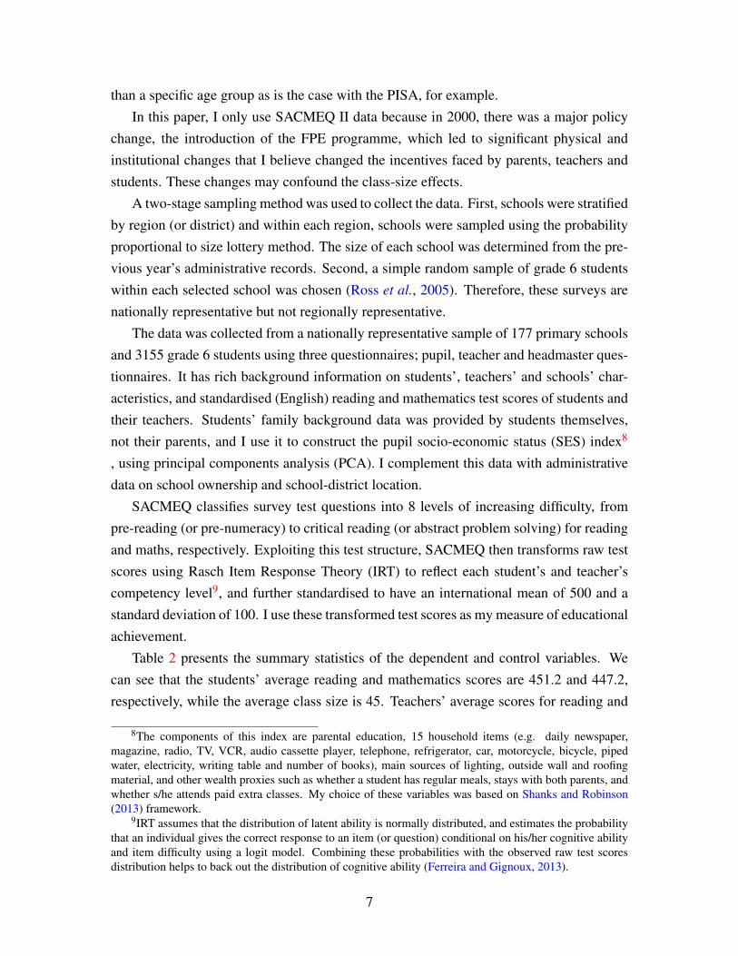
Figure 4.1: Class-size – Achievement relationship

420

440

460

480

500

Rea

ding

sco

re

20 40 60 80 100Class size

420

440

460

480

500

Mat

hs s

core

20 40 60 80 100Class size

Source: Own calculations based SACMEQ II data. Notes: The left panel shows the relationship betweenclass size and reading scores while the right panel shows that between maths scores and class size.

mathematics are 722 and 739, respectively. Even though teachers perform relatively wellin maths, students fair better in reading relative to maths. Figure 4.1 shows the relationshipbetween student test scores and class size. We can see that there is a positive relationshipbetween student achievement and class size which, taken at face value, suggests that stu-dents perform better in classes with many students.

5 Identifying Average Class Size Effects

Knowledge acquisition is generally modelled as a cumulative process that combines a fullhistory of family, community and school inputs with the child’s innate ability to producechild’s achievement as measured by test scores at a point in time (Todd and Wolpin, 2003).However, since this paper uses cross-sectional data, the empirical specification takes acontemporaneous form and is given as

Ti = λ +θSik +Xikβ + εik (5.1)

where Ti is student i’s test score, Sik is student i’s class size in school k, Xik is a vectorof child, family and other school characteristics (see Tables 2 and 3). Table 3 presentsschool characteristics summary statistics by region.

8

Table 2: Summary statistics: Pupil and teacher characteristics

Variable Mean Sd. N.Pu

pila

ndsu

bjec

t-sp

ecifi

cch

arac

teri

stic

sReading Score 451.2 57.94 3155Math score 447.2 60.36 3144Class size 44.90 18.09 3155Pupil-teacher ratio 53.85 18.49 3155Grade enrolment 70.84 54.55 3155School enrolment 616.5 384.0 3155Number of grade 6 class rooms 1.531 0.963 3155Gender (female) 0.556 0.497 3155Pupil age in months 169.63 22.15 3155Own reading textbook 0.553 0.497 3155Own math textbook 0.456 0.498 3155Share reading textbook 0.326 0.469 3155Share math textbook 0.431 0.495 3155Once repeated a class 0.608 0.488 3155SES index -1.07e-09 2.011 3155Speak English at home 0.707 0.455 3155School location (Urban) 0.351 0.477 3155

Mat

hem

atic

ste

ache

rcha

ract

eris

tics Test score 739.4 70.67 3155

Gender (female) 0.763 0.425 3146Age 40.96 9.136 3155Years of professional training 2.723 1.264 3155Years of experience 16.33 9.942 3155Teaching hours per week 23.10 6.839 3155Encourage students 0.752 0.432 3155Test frequency 1.393 0.775 3155Qualification (primary) 0.512 0.500 3155Qualification (junior secondary) 0.112 0.315 3155Qualification (Senior secondary) 0.157 0.364 3155Qualification (A-level) 0.161 0.368 3155Qualification (Tertiary) 0.0582 0.234 3155

Rea

ding

teac

herc

hara

cter

istic

s

Test score 722.0 60.19 3155Gender (female) 0.751 0.433 3146Age 41.09 9.186 3155Years of professional training 2.736 1.260 3155Years of experience 16.58 9.954 3155Teaching hours per week 22.99 6.847 3155Encourage students 0.765 0.424 3155Test frequency 1.575 0.688 3155Qualification (primary) 0.509 0.500 3155Qualification (junior secondary) 0.122 0.327 3155Qualification (Senior secondary) 0.157 0.364 3155Qualification (A-level) 0.161 0.368 3155Qualification (Tertiary) 0.0582 0.234 3155

Source: Own computations from SACMEQ (2000), SACMEQ (2007).

9

Table 3: Summary statistics: School characteristics by region

Variable N Mean Std. Dev. min maxIs

olat

edsc

hool

s School days lost 178 4.775 3.906 0 15School building condition 178 0.837 0.370 0 1

School asset index 178 4.461 1.890 1 7Sch. distance from public services 178 43.355 50.690 7.4 178

Teacher Problem Index 178 0.306 1.134 -1.754 1.952Pupil Problem Index 178 0.387 1.369 -2.222 3.160

Rur

alsc

hool

s School days lost 1871 4.904 5.836 0 33School building condition 1871 0.698 0.459 0 1

School asset index 1871 5.807 1.755 1 12Sch. distance from public services 1871 29.242 32.438 1.4 204

Teacher Problem Index 1871 0.068 1.633 -7.346 1.952Pupil Problem Index 1871 -0.134 1.565 -4.464 4.827

Tow

nsc

hool

s School days lost 797 4.302 4.942 0 20School building condition 797 0.553 0.497 0 1

School asset index 797 7.188 1.897 3 13Sch. distance from public services 797 30.731 43.703 1 280.4

Teacher Problem Index 797 0.126 1.259 -4.250 1.952Pupil Problem Index 797 -0.357 1.481 -2.268 4.591

City

scho

ols School days lost 309 4.074 4.953 0 14

School building condition 309 0.647 0.479 0 1School asset index 309 8.162 3.120 3 17

Sch. distance from public services 309 10.082 15.337 1 52.6Teacher Problem Index 309 0.020 1.373 -3.504 1.493

Pupil Problem Index 309 0.019 1.582 -1.935 4.799

All

scho

ols

zscomm01 3155 0.711 0.454 0 1zscomm02 3155 0.749 0.433 0 1zscomm03 3155 0.624 0.484 0 1zscomm04 3155 0.582 0.493 0 1zscomm05 3155 0.635 0.481 0 1zscomm06 3155 0.569 0.495 0 1zscomm07 3155 0.998 0.040 0 1zscomm08 3155 0.552 0.497 0 1zscomm09 3155 0.141 0.348 0 1

Note: School asset index is a count index made up of school ownership of assets like school library, staffroom, electricity, radio, TV, VCR, computer, etc. Pupil-Problem index and Teacher-Problem index are com-posite indices made up of problem behaviours such as pupil/teacher drug abuse, alcohol abuse, late arrivals,unjustified absenteeism, bullying of pupils/teachers, etc. zscomm01-zscomm09 are dummy variables in-dicating whether community contributes to school building, maintenance, furniture/equipment; textbook,stationery, and other materials’ purchases; payment of school fees, teacher salaries and teacher bonuses.

10

As we can see from Tables 2 and 3, there are a number of factors in Xik that are thoughtto be important to student achievement. But even after controlling for these factors, a directapplication of OLS to equation 5.1 may still give biased estimates of class size effects.A negative correlation between class size and student ability, for instance, will lead to anupward bias in the class size effect. To address this problem, I use the instrumental variablestrategy to estimate the mean and heterogeneous effects of class size. Next, I discuss theinstrument and its plausible validity.

5.1 The Instrument and its Validity

In this section, I explain how the IV is constructed from the data, and address threats toits validity, particularly issues relating to the possible violation of the exclusion restrictionrequirement.

Since the unit of analysis is the student, I use the class size associated with each studentas reported by the class teacher. This is the total number of all students in class, includingthose absent during the data collection week. I construct a regional average class size(RCL) variable, and use it as an IV for grade class size in each school. To get RCL,I exploit the fact that schools, through their respective headmasters, self-report as beingeither of the following four different locations: urban, small-urban, rural, and isolated.Therefore, I first group the schools by location in each of the ten districts. Then I calculateRCL as the average class size of each region10 and assign it to all schools within thatregion. With this IV strategy, I get 33 different regions, with 33 different average classsizes. Note that, if there is only one sampled school in a region, its class size is used toproxy the population class size of that region. For instance, some districts have one isolatedschool in the sample whose grade 6 class size is used to proxy that of all isolated schools inthat district. Isolated schools enjoy a monopoly in education supply and hence reduce thescope for parental choice, and eliminate learner sorting based on ability (Urquiola, 2006).

This IV is similar in spirit to that of Case and Deaton (1999) but the situation in Lesothois different from that that prevailed under apartheid South Africa11. Thus, there is a riskthat it is imperfectly exogenous, in which case the results we get might be worse thanthose from the OLS. Even if the circumstances were perfectly the same, this endogeneityrisk would still remain as argued by Glewwe (2002). In particular, this IV is threatened

10Here I define a region as a location within a particular district such that a rural area in District 1, forinstance, is taken as a distinct region.

11RCL IV is also similar to the average grade class size IV used by Akerhielm (1995), Asadullah (2005),Denny and Oppedisano (2013), and Woessmann and West (2006) to address within-school sorting, with thedifference being that RCL IV is the grade average class size of regional schools addressing both within- andbetween-school sorting.

11

by three things: (i) the possible presence of some region-specific omitted variables, (ii)the possibility that more motivated parents can move across regions in search of betterservices, including schools, and/or (iii) that these parents can engage in political action toskew allocation of school resources in their favour. Next I explain how I deal with the firstissue and then focus on reasons why I believe that parental actions (i.e. issues (ii) and (iii))will have a limited effect, if any, on achievement.

First, it is hard to argue against the possibility that there are some unobserved regionalfactors that can influence both regional average class size and student achievement. Someof these factors can be explained by the contagion and collective socialisation theories.According to the contagion theory, for example, when negative attitudes towards educa-tion are common within a community, such attitudes are easily taken as a norm and anyother person who behaves differently is likely to be penalised, e.g. they may be labelledas ‘acting white’ (Fryer Jr and Torelli, 2010; Nieuwenhuis et al., 2013). The collective so-cialisation theory on the other hand predicts that communities with more social cohesionare more able to enforce norms such as education importance (Nieuwenhuis et al., 2013).

The fact that problem behaviours such as drug abuse, bullying and violence are cor-related with poor educational outcomes, regional (or neighbourhood) effects on educationand class size are more likely to be mediated by these behaviours (Nieuwenhuis et al.,2013). For example, students and teachers with problematic behaviour or whose peergroups embrace such behaviour, will more likely have negative attitudes towards educa-tion, and hence put less effort into school work and skip classes (Fryer Jr and Torelli,2010). Thus these behaviours will lead to low educational outcomes. The same problem-atic behaviour can lead to low class size either due to expulsions of troublesome kids fromschool or deterring of the victimised children from attending school.

Therefore, to purge the potential influence of unobserved region-specific factors, Icontrol for such problematic behaviours of students and teachers as they reflect the char-acteristics (or attitudes towards education) of the community within which the school islocated. To achieve this, I construct Pupil-Problem index and Teacher-Problem index us-ing principal components analysis, combining problem behaviours such as pupil/teacherdrug abuse, alcohol abuse, late school arrivals, unjustified absenteeism, bullying of pu-pils/teachers, etc.12. Furthermore, I control for whether parents and/or community makecontributions to their respective schools (see Table 3).

Table 3 also shows the summary statistics of the distribution of Pupil- and Teacher-

12See Appendix Figures A.1 and A.2 for a complete list of the problem behaviours from the headmasterquestionnaire. Health problems were not included in the indices’ calculations, and all other responses wereconverted into zero-one dummies (i.e. No/Yes) by combining ‘Sometimes’ and ‘Often’ responses into a‘Yes’ response.

12

problem behaviour indices by region. Looking at this table, we indeed see that certainregions are more susceptible to certain problem behaviours than others. For example, wecan see that pupil and teacher problem behaviours are more pronounced in isolated schoolsand less pronounced in small towns and city schools, respectively. This is consistent withthe fact that pupil-teacher intimidation is prevalent in isolated schools than urban schools,for instance.

Second, with regard to cross-regional movements, much of this internal migration13

in Lesotho is largely driven by wealth and prospects of higher earnings and employmentopportunities in urban areas. It is those with high levels of education that are more likely tomove and are, in fact, disproportionately located in urban areas (see Lundahl et al., 2003).A significant portion of the society is tied to their original locations primarily by theirimmovable assets (land) and livestock, and to a lesser extent, by the risk of losing theirsocial networks which are essential to their livelihoods. To this I draw on the lessons fromthe Lesotho Highlands Water Project (LHWP) resettlement project during the constructionof the Mohale dam. Communities that were originally located in the now Mohale dambasin were given options to choose places to which they would want to be relocated. A fairnumber of households refused to relocate to urban areas (where there are better services),and chose to relocate to nearby villages (Devitt and Hitchcock, 2010).

It is hard therefore to think that families will relocate with the pure motive of searchingfor better social services while disregarding the associated economic and psychic reloca-tion costs. It is mostly those with viable alternative means of survival who are likely torelocate. Thus, it makes more sense to think that much of the pure location effect onstudent achievement operates through the household’s socio-economic status (SES).

Third, that parental tastes can influence student achievement through regional politicalaction is also likely to matter less. The argument here relies first on the way I defineregions versus political boundaries (or constituencies) and second, on school ownershipstructure through which this political pressure can potentially operate. Note that each ofthe ten districts of Lesotho has at least three constituencies, each of which is representedin parliament by a democratically elected member of parliament (MP). Therefore, giventhat resources are centrally planned, one way through which some coalition of parents canskew school resources in their favour is through their MP, who may or may not have anypolitical power in government to effect such demands. Notice the number of hurdles thischannel has to pass for it to have any chance of affecting student achievement. First thisparents-coalition would have to lobby their MP, who would then face the task of lobbying

13Here I am concerned with those who permanently relocate, not migrant labourers most of whom aretextile factory workers.

13

the cabinet to skew resources to his constituency.Even if one was to believe that this political channel is likely to occur, notice that a

region (as defined here) spans several constituencies such that rural/urban schools can bein all constituencies in any given district. Hence, taking regional (say, rural schools) av-erage resources attenuates any potential influence that parents from certain constituenciescan have on actual rural school resources. It is hard for heterogeneous groups to havea common goal. Thus, it is less likely for rural people from different constituencies toform a coalition with a common purpose of improving school resource allocation in ruralschools, for example. Moreover, some regions (e.g. rural and isolated) fall within the sameconstituency such that any favourable distribution of school resources to the constituencywill most likely equally benefit schools in different regions. This latter argument appliesagainst the potential effect of parental tastes operating through school ownership. It is hardto imagine that church authorities (i.e. school owners) could actively discriminate againstsome of their schools to the benefit of others simply because they are in different regionsof the country.

Given these arguments, it is reasonable to believe that, once one controls for SES,neighbourhood effects mediated by problem behaviour indices, and school ownership, theproposed IV is plausibly exogenous. RCL directly influences the school grade 6 classsize through which it affects the class size experienced by any individual student andthen student achievement. Put differently, school sorting strategies and parental tastes foreducation may affect the class size experienced by individual students but not the averageclass size in the school’s region.

Furthermore, in all my estimations below, I include an indicator for baseline achieve-ment (an indicator variable which is equal to one if a student has ever repeated a class),in the spirit of the value-added specifications (Todd and Wolpin, 2003, 2007). Accord-ing to Todd and Wolpin (2003), baseline achievement has persistent effects on student’sachievement in future time periods.

The plausible validity of the proposed IV allows for the estimation of the mean ef-fects of class size on educational achievement by two-stage least squares (2SLS) using thefollowing system:

Tik = λ +θSk +Xikβ +υik (5.2)

Sk = γRCLk +Xikβ + εk (5.3)

where RCLk is regional class size instrumenting for grade class size in school k, Sk, and

14

Xik is a vector of all other exogenous factors.

5.2 Empirical Estimates of Average Class Size Effects

In this section, I test whether class-size has any effect on students’ achievement. First, Ipresent evidence on the impact of class size on average achievement and then present sens-itivity analysis results where I allow for possible violations of the IV exclusion restrictionrequirement.

5.3 OLS and Two-Stage Least Squares results

Table 4 reports the OLS and 2SLS estimates for the average effect of class size on stu-dent achievement. Columns (1) and (2) of this table show the OLS results for reading andmaths scores, respectively. In column (1), we can see that reading scores are negativelycorrelated with class size. Results in column (2) however indicate that maths scores arepositively correlated with class size. For instance, these coefficients respectively implythat a one student increase in class size is associated with a 0.06 points decrease in read-ing scores and a 0.18 points increase in maths scores. Even though they are statisticallyinsignificant, we can clearly see that once we include controls in our model, the seeminglystrong positive relationship between test scores and class size seen in Figure 4.1 is attenu-ated for maths scores and even reversed in the case of reading scores. This is an indicationthat introducing these controls removes some bias in OLS results.

As expected, teacher subject-knowledge is positively related with student achievementin both reading and maths, but children’s socioeconomic background is only positivelyrelated with reading performance and not with maths. Grade repetition has a negativerelation with student performance. For instance, pupil who have once repeated a gradescore almost 16 and 10 points, in reading and maths respectively, below those who havenot repeated a grade.

School location is a dummy that equals one if a school is in a city or small town (urban),and zero otherwise(i.e. if it is in a rural or isolated location). We can also see from the OLSresults that urban schools perform better than rural schools. Further, school ownership isalso important for achievement: government schools perform relatively better than allchurch-owned schools. Looking at columns 3 and 5 results, it turns out that church-ownedschools also have relatively higher class sizes than government schools which potentiallyexplains their relatively lower performance. This indicates a possible negative class sizeeffect on achievement.

To address the potential endogeneity problem, I estimated the 2SLS regression model,

15

instrumenting class size with regional average class size for grade 614. The results arepresented in columns (3) to (6) of Table 4. In both the first-stage and second-stage re-gressions, the same control variables were included. The lower part of Table 4 reports firststage regressions’ diagnostic and identification statistics. We can see from columns (3) and(5) that the Kleibergen-Paap Wald rk F-statistic is equal to 55.65 (for reading scores) and72.97 (for maths scores)15. These figures are far greater than the rule of thumb value of 10thereby indicating that our instrument, i.e. regional average class size, strongly predictsclass size (Staiger and Stock, 1997).

Columns (4) and (6) present the IV (second-stage regression) results for reading andmaths scores, respectively. Overall the results indicate that class size has a negative effecton student achievement. In column (4), we see that reducing class size by one pupil raisesan average student’s reading score by 1.22 points, and this effect is statistically significantat 1% level. In standard deviation form, this implies that a one standard deviation reductionin class size (approximately 18 students) increases average reading scores by 0.38 standarddeviations. Using an eight-students reduction in class size as in Angrist and Lavy (1999)and Urquiola (2006), I find an effect size of 0.17 standard deviations (almost 10 pointsincrease), which is in the range of the effect size reported by Angrist and Lavy (1999), andalmost equal to the 0.16 standard deviation effect on reading scores reported by Urquiola(2006). By all standards, this is a sizeable effect16.

In column (6), results indicate that reducing class size by one standard deviation leadsto 0.12 standard deviations increase in maths scores. However, this class size effect isstatistically insignificant. The fact that class size only benefits an average student in Eng-lish reading is possibly explained by the fact that teaching maths requires relatively lesspupil-teacher interaction compared to teaching English reading. Students require muchmore attention from the teacher to learn English as a second language, and use the skillsto comprehend English questions, than in learning maths. Comparing these IV regressionresults with the OLS regression results, we can see that the OLS coefficients are biasedupwards.

14As a robustness check, I constructed the modified RCL IV by leaving out own school class size (exceptfor isolated schools) such that for three schools in a region, for instance, the average class size of the othertwo schools is used to instrument that of the left out school. The results are similar to what we present here.See Table A1. I am very grateful to the anonymous referee for suggesting this RCL IV construction.

15The corresponding Cragg-Donald Wald F-statistics, respectively, are 607.13 and 814.44.16Fredriksson et al. (2013) report an effect size of 0.23 standard deviations on cognitive skills using a

seven students reduction in class size. I get an effect size of 0.15 standard deviations using the same classsize reduction.

16

Tabl

e4:

OL

San

d2S

LS

estim

ates

forC

lass

size

effe

cton

achi

evem

ent

OL

SR

esul

ts2S

LS

Res

ults

(1)

(2)

(3)

(4)

(5)

(6)

VAR

IAB

LE

SR

eadi

ngSc

ores

Mat

hsSc

ores

Rea

ding

Scor

esM

aths

Scor

esFi

rst-

stag

eSe

cond

-sta

geFi

rst-

stag

eSe

cond

-sta

geR

eadi

ngsc

ore

Mat

hssc

ore

Cla

sssi

zeR

eadi

ngsc

ore

Cla

sssi

zeM

aths

scor

eC

lass

size

-0.0

622

0.17

6-1

.219

***

-0.3

94(0

.195

)(0

.210

)(0

.395

)(0

.325

)IV

:Reg

iona

lCla

sssi

ze0.

925*

**1.

055*

**(0

.041

8)(0

.055

4)Te

ache

rsco

re0.

0895

**0.

0835

***

0.04

04**

*0.

142*

**0.

0634

***

0.11

0***

(0.0

423)

(0.0

310)

(0.0

0507

)(0

.047

4)(0

.005

61)

(0.0

418)

Text

book

acce

ss2.

273

-3.9

09-1

.221

*2.

875

-2.3

46**

*-4

.313

(3.3

56)

(3.2

61)

(0.6

56)

(4.0

57)

(0.5

83)

(3.4

45)

Pupi

lRep

eate

d-1

5.80

***

-10.

20**

*0.

849

-14.

86**

*0.

472

-9.9

42**

*(2

.834

)(2

.374

)(0

.617

)(3

.012

)(0

.601

)(2

.384

)SE

Sin

dex

1.81

2**

-0.8

000.

108

2.14

9**

0.13

8-0

.597

(0.8

23)

(0.7

94)

(0.1

59)

(0.9

59)

(0.1

58)

(0.8

19)

Scho

ollo

catio

n(u

rban

)11

.48*

*20

.44*

**-2

.758

***

18.5

9***

-3.8

87**

*24

.10*

**(5

.653

)(5

.509

)(0

.944

)(7

.215

)(0

.947

)(6

.572

)C

omm

unity

Scho

ol-9

7.28

***

-122

.0**

*39

.42*

**-4

2.35

47.3

6***

-91.

05**

*(3

1.51

)(2

7.99

)(3

.344

)(3

6.82

)(4

.138

)(3

5.07

)R

CC

Scho

ol-1

11.7

***

-113

.5**

*28

.74*

**-7

6.40

**35

.20*

**-9

3.28

***

(29.

49)

(25.

87)

(3.2

04)

(31.

86)

(3.8

20)

(29.

25)

LE

CSc

hool

-114

.0**

*-1

17.6

***

30.1

3***

-78.

81**

38.4

8***

-96.

45**

*(2

9.38

)(2

6.42

)(3

.211

)(3

0.95

)(3

.849

)(2

9.92

)A

CL

Scho

ol-1

01.2

***

-104

.1**

*39

.34*

**-5

4.41

47.0

1***

-78.

00**

(28.

99)

(26.

22)

(3.3

91)

(35.

33)

(3.9

31)

(35.

09)

AM

ESc

hool

-115

.5**

*-1

08.7

***

16.8

9***

-88.

36**

*23

.86*

**-9

2.22

***

(31.

10)

(24.

69)

(3.5

02)

(34.

28)

(4.3

35)

(28.

26)

Oth

erC

hurc

hes

scho

ol-6

9.03

*-7

8.28

***

24.4

7***

-41.

8931

.07*

**-6

1.99

**(3

8.78

)(2

7.38

)(3

.823

)(3

6.43

)(4

.944

)(2

8.49

)C

onst

ant

568.

3***

596.

4***

-98.

75**

*49

1.4*

**-1

19.3

***

555.

2***

(45.

41)

(49.

50)

(7.3

99)

(62.

81)

(8.4

44)

(66.

62)

Obs

erva

tions

3,14

63,

135

3,14

63,

146

3,13

53,

135

R-s

quar

ed0.

229

0.17

60.

444

0.14

20.

470

0.15

3Fi

rst-

stag

ere

gres

sion

ssu

mm

ary

stat

istic

sK

leib

erge

n-Pa

apW

ald

rkF

stat

istic

55.6

572

.97

Shea

part

ialR

20.

164

0.20

8N

otes

:All

regr

essi

onsh

ave

cont

rolle

dfo

rall

othe

rind

ivid

ual,

scho

olan

dfa

mily

char

acte

rist

ics(

e.g.

teac

her’

squa

lifica

tion,

year

sofe

xper

ienc

e,ye

arso

fpro

fess

iona

ltr

aini

ng,s

ex,a

ndag

e;te

achi

ngho

urs,

teac

her

and

pupi

lgen

der,

pupi

lage

and

hom

ela

ngua

ge).

Gov

ernm

ents

choo

lsar

eth

eom

itted

cate

gory

.R

obus

tSta

ndar

der

rors

(clu

ster

edat

scho

olle

vel)

are

inpa

rent

hese

s.Si

gnifi

canc

ele

vels

:***

sign

ifica

ntat

1pe

rcen

t,**

sign

ifica

ntat

5pe

rcen

t,*s

igni

fican

tat1

0pe

rcen

t.

17

5.4 Sensitivity Analysis

I acknowledge that it is hard (if not impossible) to entirely dispel the cloud of invalidityever-hanging over my IV, even after controlling for all possible correlates of achievement.Thus, in this Section I perform some sensitivity analysis in order to empirically assess itsvalidity, and show that the causal inferences about class size effect on achievement madein the above section are credible. To this end, I adopt two bounds methods by Conley et al.

(2012) that allow one to draw inferences when the IV potentially violates the exogeneityrestriction.

The first method is the union of confidence intervals (UCI). This approach allows oneto examine the robustness of the results to the presence of a direct relationship between theIV (i.e. regional class size) and the outcome (i.e. student achievement), regardless of themechanisms through which this may occur. To achieve this, Conley et al. (2012) modifythe simultaneous equation system presented in equations 5.2 and 5.3 as follows:

Tik = λ +θSk + γRCLk +Xikβ +υik (5.4)

Sk = γRCLk +Xikβ + εk (5.5)

The difference between this model and the normal two-stage IV model defined in equa-tions 5.2 and 5.3 is the presence of the term, γRCLk, in the structural equation 5.4. Understrict exogeneity assumption, the requirement is that regional class size have no direct in-fluence on achievement, i.e. γ = 0. The Conley et al.’s (2012) UCI approach amountsto relaxing this strict requirement such that γ 6= 0, and then checking the significance ofour main results. As I have argued in Section 5.1 above, even if γ 6= 0, there is reason tobelieve that it is small. Assume that γ = γ0, equation 5.2 becomes

(Tik− γ0RCLk) = λ +θSk +Xikβ +υik (5.6)

This implies that RCLk is now a valid IV for Sk when the outcome variable is (Tik−γ0RCLk). Hence we can consistently estimate θ by two-stage least squares method us-ing RCLk as an instrument for Sk. Under the union of confidence intervals aproach, γ isassumed to have some specific support interval, γ ∈ [−δ ,+δ ], since we do not know itstrue value, and then the union of intervals for θ is estimated given any γ0 in that interval.Conley et al. (2012) note that, as long as γ ∈ [−δ ,+δ ], the union will contain the trueparameter value of θ with an asymptotic probability Pr[θ ∈CIN(1−α)] ≥ 1−α , whereCIN(1−α) is the 95% confidence interval for θ . That is, CIN(1−α) will asymptotically

18

contain the true class size effect, θ , at least 95% of the time.The second method is the γ-Local-to-Zero approximation bounds method. Under this

approach, the exclusion restriction requirement is relaxed by allowing for uncertainty inour priors about γ . This is equivalent to introducing some bias term or ‘exogeneity error’(Aγ) in the approximate distribution of θ ;

θapprox∼ N(θ ,V2SLS)+Aγ (5.7)

A = (X ′PZX)−1X ′Z

γ ∼ F

where V2SLS is the variance-covariance matrix for 2SLS, Z is the IV, PZ = Z(Z′Z)−1Z′,and F is the distribution of γ . Thus the distribution of the exogeneity error is dependent onthe sample moments of matrix A17 and the distribution F , and reflects the deviations of θ

from the asymptotic standard distribution of the 2SLS estimator caused by violations of theexclusion restriction assumption. In here I assume that γ follows a normal distribution withmean µγ and variance Ωγ such that the approximate distribution of the interest parameteris given as

θapprox∼ N(θ +Aµγ ,V2SLS +AΩγA′) (5.8)

In the implementation, I apply the simplest form of priors about γ which is that γ ∼N(0,δ 2), and compute the 95% confidence intervals for θ corresponding to different val-ues of δ , as in Conley et al. (2012); Dang (2013) and Mancusi and Vezzulli (2014). Ac-cording to Conley et al. (2012), this approach gives valid inference under the assumptionthat our priors are correct, and provides robustness relative to the normal 2SLS approach.

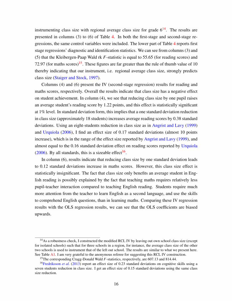
The sensitivity results are shown in Figure 5.1. This Figure specifically shows the 95%confidence bounds of the IV coefficient, θ , using Conley et al.’s (2012) UCI and LTZ con-fidence bounds methods. Results for maths scores are presented in Figure 5.1a and thosefor reading scores are shown in Figure 5.1b. In these Figures, we have a straight solid lineat θ = 0 (the zero-line). The solid horizontal line below the zero-line shows the 2SLS classsize effect estimates for the respective test scores. The two dash lines around the 2SLS es-timates represent the lower and upper limits of the respective test scores. Therefore, oncethe 95% upper limit crosses the zero-line, that is once confidence bounds include the zero-effect, the 2SLS estimates are no longer significant at 5% level of significance. But if the

17Notice that, since the size of A is inversely related to the projection matrix PZ , the influence of theexogeneity error on θ is negatively related with the strength of the IV, Z (see Conley et al., 2012).

19

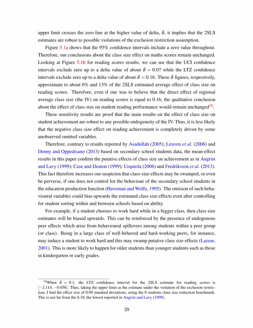
upper limit crosses the zero-line at the higher value of delta, δ , it implies that the 2SLSestimates are robust to possible violations of the exclusion restriction assumption.

Figure 5.1a shows that the 95% confidence intervals include a zero value throughout.Therefore, our conclusions about the class size effect on maths scores remain unchanged.Looking at Figure 5.1b for reading scores results, we can see that the UCI confidenceintervals exclude zero up to a delta value of about δ = 0.07 while the LTZ confidenceintervals exclude zero up to a delta value of about δ = 0.16. These δ figures, respectively,approximate to about 6% and 13% of the 2SLS estimated average effect of class size onreading scores. Therefore, even if one was to believe that the direct effect of regionalaverage class size (the IV) on reading scores is equal to 0.16, the qualitative conclusionabout the effect of class size on student reading performance would remain unchanged18.

These sensitivity results are proof that the main results on the effect of class size onstudent achievement are robust to any possible endogeneity of the IV. Thus, it is less likelythat the negative class size effect on reading achievement is completely driven by someunobserved omitted variables.

Therefore, contrary to results reported by Asadullah (2005); Leuven et al. (2008) andDenny and Oppedisano (2013) based on secondary school students data, the mean-effectresults in this paper confirm the putative effects of class size on achievement as in Angristand Lavy (1999); Case and Deaton (1999); Urquiola (2006) and Fredriksson et al. (2013).This fact therefore increases our suspicion that class-size effects may be swamped, or evenbe perverse, if one does not control for the behaviour of the secondary school students inthe education production function (Haveman and Wolfe, 1995). The omision of such beha-vioural variables could bias upwards the estimated class size effects even after controllingfor student sorting within and between schools based on ability.

For example, if a student chooses to work hard while in a bigger class, then class sizeestimates will be biased upwards. This can be reinforced by the presence of endogenouspeer effects which arise from behavioural spillovers among students within a peer group(or class). Being in a large class of well-behaved and hard-working peers, for instance,may induce a student to work hard and this may swamp putative class size effects (Lazear,2001). This is more likely to happen for older students than younger students such as thosein kindergarten or early grades.

18When δ = 0.1, the LTZ confidence interval for the 2SLS estimate for reading scores is[−2.114,−0.056]. Thus, taking the upper limit as the estimate under the violation of the exclusion restric-tion, I find the effect size of 0.09 standard deviations, using the 8 students class size reduction benchmark.This is not far from the 0.10, the lowest reported in Angrist and Lavy (1999).

20

Figure 5.1: Conley-Hansen-Rossi bounds test for instrument validity(a) IV validity in maths test scores regressions

−1

−.5

0.5

1T

heta

.05 .1 .15 .2Delta

Upper Bound (UCI) Lower Bound (UCI)

UCI 95% bounds for Maths scores

−1

−.5

0.5

1T

heta

0 .05 .1 .15 .2Delta

Point Estimate (LTZ) CI (LTZ)

LTZ 95% bounds for Maths scores

(b) IV validity in reading test scores regressions

−2.

5−

2−

1.5

−1

−.5

0T

heta

.05 .1 .15 .2Delta

Upper Bound (UCI) Lower Bound (UCI)

UCI 95% bounds for Reading scores

−2.

5−

2−

1.5

−1

−.5

0T

heta

0 .05 .1 .15 .2Delta

Point Estimate (LTZ) CI (LTZ)

LTZ 95% bounds for Reading scores

Notes: The Union of Confidence Intervals (UCI) bounds are drawn for varying levels of delta, which definethe support of the gamma parameter (i.e. the true direct effect of regional average class size on achievement).The γ-Local-to-Zero Approximation (LTZ) bounds are drawn for varying values of delta under the assump-tion that γ ∼N(0,δ 2) (see Conley et al., 2012). All the reported bounds are for the 95% confidence intervalswhich have been generated from robust school-level clustered standard errors. The estimates are performedusing a STATA code ‘plausexog’ by Damian Clarke downloadable via ssc install plausexog.

21

6 Estimating the Distributional Effects of Class Size onAchievement

Having shown the robustness of the mean effects, in this section I first deal with estimatingthe distributional effects of class size on student achievement and then present the results.

6.1 The Instrumental Variable Quantile Regression Model of Achieve-ment

To analyse the distributional effects of class size on achievement, I adopt the instrumentalvariable quantile regression (IVQR) model developed by Chernozhukov and Hansen (2005,2006, 2008). Let Ts be potential school outcomes indexed against potential values s of theendogenous variable S. Let capital letters denote random variables and lowercase lettersdenote the values these random variables may take. For example, Ts is student test scorewhen (class-size) S = s. The prime objects of interest are the conditional quantiles of po-tential test scores given class size s and quantile index τ , denoted as q(s,x,τ), and quantiletreatment effects (QTE) which give the difference between the quantiles of Ts under dif-ferent levels of s, given as

q(s,x,τ)−q(s′,x,τ) or

∂q(s,τ)∂ s

(for a continuous treatment s). (6.1)

Conditional on observed student and school characteristics X = x, Ts is related to itsquantile function q(s,x,τ) as

Ts = q(s,x,Us) (6.2)

where Us ∼U(0,1) is the rank variable that captures heterogeneity of test scores for stu-dents with observationally similar characteristics, x, and treatment status s. Us also de-termines each student’s relative rank in terms of potential test scores and thus, can also bethought of as representing student ability.

Given that class size is endogenous, one needs a set of valid instrumental variables, Z,in order to get its QTE. In this paper, Z represents the plausibly exogenous IV, regionalaverage class size. Thus, one has the following structural model

T = S′θ(U)+X

′β (U) (6.3)

S = ϕ(X,Z,V ) (6.4)

22

where U |X,Z ∼U(0,1), ϕ is some unknown function, and V is a random vector that isstatistically dependent on U . When U = τ , the linear conditional quantile function thatone wishes to estimate is given as

q(S,X,τ) = S′θ(τ)+X

′β (τ), τ ∈ (0,1) (6.5)

where q(S,X,τ) denotes the τ th quantile of test score, Ti, given a dim(β (τ))-vector ofexogenous variables, X, at τ th quantile, S is a dim(θ(τ))-vector of possibly endogenousvariables at the τ th quantile, and q(·) is strictly increasing in individual’s pure cognitiveability, τ .

The main assumption required for the estimation of the QTE is rank similarity19, mean-ing that Us is equal in distribution to Us′ conditional on V (i.e. Us ∼Us′). This implies thatthe treatment machanism does not lead to systematic changes in students ranks acrosspotential outcomes.

The main statistical implication of the model is therefore that

P[T ≤ q(S,X,τ)|X,Z] = P[T −S′θ(τ)−X

′β (τ)≤ 0|X,Z] = τ (6.6)

deriving from the fact that T ≤ q(S,X,τ) ≡ U ≤ τ under the rank invariance (or ranksimilarity) assumption. Equation 6.6 is the main equation for identification. It implies that0 is the τ th quantile of the random variable T −S′θ(τ)−X′β (τ) conditional on X and Z20.

Thus the IVQR problem for (θ(τ),β (τ)) is the solution to the following minimizationproblem:

0 = arg min︸ ︷︷ ︸ψτ

1n

n

∑i=1

ρτ

(Ti−S

′iθ(τ)−X

′iβ (τ)−Z

′iγ(τ)

)(6.7)

where ψτ =

θ(τ)′,β (τ)

′

and ρτ(u) = (τ−1(u≤ 0))u is the asymmetric least ab-solute loss (i.e. the “check function”) (Angrist and Pischke, 2009). An estimate for θ(τ),θ(τ), is that that drives the coefficient of the IV, γ(τ), as close to zero as possible in anordinary quantile regression of Ti−S′iθ(τ) on X and Z since the IV should only affect thetest scores via its effect on class size. That is,

θ(τ) = arg inf︸ ︷︷ ︸θ∈A

n[γ(θ ,τ)′]A(θ)[γ(θ ,τ)] (6.8)

19The stronger version of this assumption is rank invariance which, in here, implies that a student’spercentile rank in the test score distribution when class size S = s is the same as when class size S = s′.

20That is 0 = QT−q(S,X,τ)(τ|X,Z), asymptotically, for each τ .

23

where A is the parameter space for θ , A(θ) = A(θ) + op(1) and A(θ) is any uni-formly positive definite matrix in θ ∈ A . In practice, A(θ) is equal to the variance-covariance matrix of

√n(γ(θ ,τ)− γ(θ ,τ)) such that Wn(θ) = n[γ(θ ,τ)

′]A(θ)[γ(θ ,τ)] is

the Wald statistic for testing γ(θ ,τ) = 0. The parameter estimates are therefore given by(θ(τ), β (τ)

)=(

θ(τ), β (θ(τ),τ))

(see Chernozhukov and Hansen, 2006).

6.2 Estimates of Distributional Effects of Class Size21

Here I present results on the distributional effects of class size on student achievement.Table 5 and the left panel of Figure 6.1 present results on the effect of class size on studentreading performance from the 5th quantile to the 95th quantile of the reading scores distri-bution. We can see from the Table that class size has a negative and statistically significanteffect on the reading performance of students across all quantiles of the reading scores dis-tribution. The effect is much stronger for low-ability students’ performance (i.e. for thoseat lower quantiles) and declines as we move up the quantiles. For instance, for students atthe 5th quantile of the reading scores distribution, the estimates suggest that reducing classsize by eight students improves their reading performance by 0.21 standard deviations.The effect size is 0.19 and 0.10 standard deviations increase in reading performance ofstudents at the 55th quantile and 85th quantile, respectively.

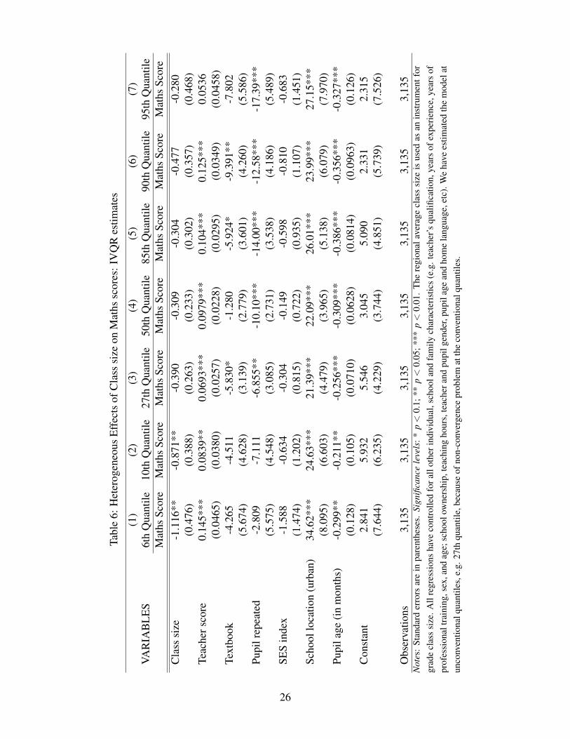
Table 6 and the right panel of Figure 6.1 show results on the distributional effectsof class size on students’ maths performance. Consistent with reading scores class sizeeffects, class size benefits lower-ability students the most. But unlike the reading results,the estimated class size effects are only significant for students below the 20th quantile,and above this threshold, class size effects on maths performance dissipate. Reducing classsize by eight pupils raises maths scores of students who are at the 6th and 10th quantile,respectively, by 0.15 and 0.12 standard deviations. These are fairly large effects, and as Ipointed out earlier, they are very much in the range of the magnitudes reported elsewherein the literature.

The evidence that low-ability students benefit more from small classes is consistentwith results by Robinson (1990) and Eide and Showalter (1998) but is at odds with that byKonstantopoulos (2007). These results imply that a policy that reduces class size holds thepromise of increasing education quality and simultaneously reducing educational inequal-ity. The fact that class size on maths performance is beneficial to only those at the very endof the of the ability scale highlights that looking at the average effects of class size mayactually gloss over the offsetting effects at different parts of the achievement distribution.

21Estimation is performed in Stata using a code developed by Don Won Kwak and available for downloadat http://faculty.chicagobooth.edu/christian.hansen/research/.

24

Tabl

e5:

Het

erog

eneo

usE

ffec

tsof

Cla

sssi

zeon

read

ing

scor

es:I

VQ

Res

timat

es

VAR

IAB

LE

S(1

)(2

)(3

)(4

)(5

)(6

)(7

)5t

hQ

uant

ile11

thQ

uant

ile15

thQ

uant

ile55

thQ

uant

ile75

thQ

uant

ile85

thQ

uant

ile95

thQ

uant

ileR

ead

Scor

eR

ead

Scor

eR

ead

Scor

eR

ead

Scor

eR

ead

Scor

eR

ead

Scor

eR

ead

Scor

eC

lass

size

-1.5

32**

*-1

.474

***

-1.6

54**

*-1

.398

***

-0.8

45**

*-0

.729

***

-0.9

23**

(0.4

62)

(0.3

37)

(0.3

13)

(0.2

22)

(0.2

35)

(0.2

81)

(0.4

62)

Teac

hers

core

-0.0

0943

0.06

65*

0.07

57**

0.14

6***

0.15

4***

0.14

0***

0.20

8***

(0.0

509)

(0.0

371)

(0.0

344)

(0.0

245)

(0.0

258)

(0.0

309)

(0.0

508)

Text

book

2.82

7-1

.256

2.32

31.

814

1.46

72.

855

11.0

4**

(5.4

52)

(3.9

74)

(3.6

88)

(2.6

22)

(2.7

69)

(3.3

12)

(5.4

45)

Pupi

lrep

eate

d-5

.687

-6.9

56*

-7.7

20**

-13.

92**

*-2

0.17

***

-27.

70**

*-3

6.10

***

(5.4

04)

(3.9

39)

(3.6

55)

(2.5

99)

(2.7

44)

(3.2

83)

(5.3

96)

SES

inde

x-0

.639

0.70

21.

528

2.58

4***

2.43

0***

2.66

1***

3.96

5***

(1.4

23)

(1.0

37)

(0.9

63)

(0.6

84)

(0.7

23)

(0.8

65)

(1.4

21)

Scho

ollo

catio

n(u

rban

)22

.07*

**20

.91*

**21

.65*

**18

.99*

**17

.85*

**16

.22*

**24

.53*

**(7

.667

)(5

.588

)(5

.186

)(3

.687

)(3

.894

)(4

.658

)(7

.656

)Pu

pila

ge(i

nm

onth

s)-0

.242

*-0

.327

***

-0.2

79**

*-0

.326

***

-0.4

27**

*-0

.452

***

-0.3

02**

(0.1

24)

(0.0

905)

(0.0

840)

(0.0

597)

(0.0

631)

(0.0

754)

(0.1

24)

Con

stan

t-3

.186

0.56

82.

225

7.36

3**

11.9

5***

10.1

8**

12.5

1*(7

.369

)(5

.372

)(4

.985

)(3

.544

)(3

.743

)(4

.477

)(7

.359

)

Obs

erva

tions

3,14

63,

146

3,14

63,

146

3,14

63,

146

3,14

6N

otes

:St

anda

rder

rors

are

inpa

rent

hese

s.Si

gnifi

canc

ele

vels

:*p<

0.1;

**p<

0.05

;***

p<

0.01

.T

here

gion

alav

erag

ecl

ass

size

isus

edas

anin

stru

men

tfor

grad

ecl

ass

size

.All

regr

essi

ons

have

cont

rolle

dfo

rall

othe

rind

ivid

ual,

scho

olan

dfa

mily

char

acte

rist

ics

(e.g

.tea

cher

’squ

alifi

catio

n,ye

ars

ofex

peri

ence

,yea

rsof

prof

essi

onal

trai

ning

,sex

,and

age;

scho

olow

ners

hip,

teac

hing

hour

s,te

ache

rand

pupi

lgen

der,

pupi

lage

and

hom

ela

ngua

ge,e

tc).

We

have

estim

ated

the

mod

elat

unco

nven

tiona

lqua

ntile

s,e.

g.11

thqu

antil

e,be

caus

eof

non-

conv

erge

nce

prob

lem

atth

eco

nven

tiona

lqua

ntile

s.

25

Tabl

e6:

Het

erog

eneo

usE

ffec

tsof

Cla

sssi

zeon

Mat

hssc

ores

:IV

QR

estim

ates

VAR

IAB

LE

S(1

)(2

)(3

)(4

)(5

)(6

)(7

)6t

hQ

uant

ile10

thQ

uant

ile27

thQ

uant

ile50

thQ

uant

ile85

thQ

uant

ile90

thQ

uant

ile95

thQ

uant

ileM

aths

Scor

eM

aths

Scor

eM

aths

Scor

eM

aths

Scor

eM

aths

Scor

eM

aths

Scor

eM

aths

Scor

eC

lass

size

-1.1

16**

-0.8

71**

-0.3

90-0

.309

-0.3

04-0

.477

-0.2

80(0

.476

)(0

.388

)(0

.263

)(0

.233

)(0

.302

)(0

.357

)(0

.468

)Te

ache

rsco

re0.

145*

**0.

0839

**0.

0693

***

0.09

79**

*0.

104*

**0.

125*

**0.

0536

(0.0

465)

(0.0

380)

(0.0

257)

(0.0

228)

(0.0

295)

(0.0

349)

(0.0

458)

Text

book

-4.2

65-4

.511

-5.8

30*

-1.2

80-5

.924

*-9

.391

**-7

.802

(5.6

74)

(4.6

28)

(3.1

39)

(2.7

79)

(3.6

01)

(4.2

60)

(5.5

86)

Pupi

lrep

eate

d-2

.809

-7.1

11-6

.855

**-1

0.10

***

-14.

00**

*-1

2.58

***

-17.

39**

*(5

.575

)(4

.548

)(3

.085

)(2

.731

)(3

.538

)(4

.186

)(5

.489

)SE

Sin

dex

-1.5

88-0

.634

-0.3

04-0

.149

-0.5

98-0

.810

-0.6

83(1

.474

)(1

.202

)(0

.815

)(0

.722

)(0

.935

)(1

.107

)(1

.451

)Sc

hool

loca

tion

(urb

an)

34.6

2***

24.6

3***

21.3

9***

22.0

9***

26.0

1***

23.9

9***

27.1

5***

(8.0

95)

(6.6

03)

(4.4

79)

(3.9

65)

(5.1

38)

(6.0

79)

(7.9

70)

Pupi

lage

(in

mon

ths)

-0.2

99**

-0.2

11**

-0.2

56**

*-0

.309

***

-0.3

86**

*-0

.356

***

-0.3

27**

*(0

.128

)(0

.105

)(0

.071

0)(0

.062

8)(0

.081

4)(0

.096

3)(0

.126

)C

onst

ant

2.84

15.

932

5.54

63.

045

5.09

02.

331

2.31

5(7

.644

)(6

.235

)(4

.229

)(3

.744

)(4

.851

)(5

.739

)(7

.526

)

Obs

erva

tions

3,13

53,

135

3,13

53,

135

3,13

53,

135

3,13

5N

otes

:St

anda

rder

rors

are

inpa

rent

hese

s.Si

gnifi

canc

ele

vels

:*p<

0.1;

**p<

0.05

;***

p<

0.01

.T

here

gion

alav

erag

ecl

ass

size

isus

edas

anin

stru

men

tfor

grad

ecl

ass

size

.All

regr

essi

ons

have

cont

rolle

dfo

rall

othe

rind

ivid

ual,

scho

olan

dfa

mily

char

acte

rist

ics

(e.g

.tea

cher

’squ

alifi

catio

n,ye

ars

ofex

peri

ence

,yea

rsof

prof

essi

onal

trai

ning

,sex

,and

age;

scho

olow

ners

hip,

teac

hing

hour

s,te

ache

rand

pupi

lgen

der,

pupi

lage

and

hom

ela

ngua

ge,e

tc).

We

have

estim

ated

the

mod

elat

unco

nven

tiona

lqua

ntile

s,e.

g.27

thqu

antil

e,be

caus

eof

non-

conv

erge

nce

prob

lem

atth

eco

nven

tiona

lqua

ntile

s.

26

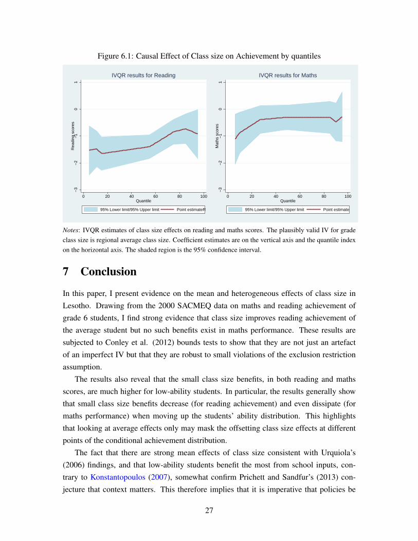
Figure 6.1: Causal Effect of Class size on Achievement by quantiles

−3

−2

−1

01

Rea

ding

sco

res

0 20 40 60 80 100Quantile

95% Lower limit/95% Upper limit Point estimateR

IVQR results for Reading

−3

−2

−1

01

Mat

hs s

core

s

0 20 40 60 80 100Quantile

95% Lower limit/95% Upper limit Point estimate

IVQR results for Maths

Notes: IVQR estimates of class size effects on reading and maths scores. The plausibly valid IV for gradeclass size is regional average class size. Coefficient estimates are on the vertical axis and the quantile indexon the horizontal axis. The shaded region is the 95% confidence interval.

7 Conclusion

In this paper, I present evidence on the mean and heterogeneous effects of class size inLesotho. Drawing from the 2000 SACMEQ data on maths and reading achievement ofgrade 6 students, I find strong evidence that class size improves reading achievement ofthe average student but no such benefits exist in maths performance. These results aresubjected to Conley et al. (2012) bounds tests to show that they are not just an artefactof an imperfect IV but that they are robust to small violations of the exclusion restrictionassumption.

The results also reveal that the small class size benefits, in both reading and mathsscores, are much higher for low-ability students. In particular, the results generally showthat small class size benefits decrease (for reading achievement) and even dissipate (formaths performance) when moving up the students’ ability distribution. This highlightsthat looking at average effects only may mask the offsetting class size effects at differentpoints of the conditional achievement distribution.

The fact that there are strong mean effects of class size consistent with Urquiola’s(2006) findings, and that low-ability students benefit the most from school inputs, con-trary to Konstantopoulos (2007), somewhat confirm Prichett and Sandfur’s (2013) con-jecture that context matters. This therefore implies that it is imperative that policies be

27

designed based on context-specific evidence. In the light of this evidence, I can safelyargue that Lesotho’s policy of reducing pupil-teacher ratio holds promise of increasing av-erage education quality and potentially closing the performance gap between the low andhigh ability students.

The hard question remains whether the reported effect sizes are of sufficient mag-nitudes to make class size reductions a cost-effective policy option or whether the shortterm costs outweigh the long term benefits. Currently, there is no outside data to answerthis question. To make judgement on whether class size reduction is a better policy option,one would need information on achievement effect of other feasible policy options such asprovision of textbook. To do cost-benefit analysis, one would need information on otherdirect benefits of class size (e.g. its effect on drop-out rates) and indirect benefits (e.g. itseffect on wages). These questions still require further research.

28

References

Akerhielm, K. (1995) Does class size matter?, Economics of Education Review, 14, 229–241.

Ambrose, D. (2007) The History of Education in Lesotho: Six Brief Subsectoral Studies,Lesotho Miscelaneous Documents, No. 23.

Ammermueller, A. (2007) PISA: What makes the difference?: Explaining the gap in testscores between Finland and Germany., Empirical Economics, 33, 263–287.

Angrist, J. D. and Lavy, V. (1999) Using Maimonides’ rule to estimate the effect of classsize on scholastic achievement, The Quarterly Journal of Economics, 114, 533–575.

Angrist, J. D. and Pischke, J.-S. (2009) Mostly harmless econometrics: An empiricist’s

companion, Princeton University Press, New Jersey.

Asadullah, M. N. (2005) The effect of class size on student achievement: evidence fromBangladesh, Applied Economics Letters, 12, 217–221.

Case, A. and Deaton, A. (1999) School inputs and educational outcomes in South Africa,The Quarterly Journal of Economics, 114, 1047–1084.

Chernozhukov, V. and Hansen, C. (2005) An IV model of quantile treatment effects, Eco-

nometrica, 73, 245–261.

Chernozhukov, V. and Hansen, C. (2006) Instrumental quantile regression inference forstructural and treatment effect models, Journal of Econometrics, 132, 491–525.

Chernozhukov, V. and Hansen, C. (2008) Instrumental variable quantile regression: Arobust inference approach, Journal of Econometrics, 142, 379–398.

Conley, T. G., Hansen, C. B. and Rossi, P. E. (2012) Plausibly exogenous, Review of

Economics and Statistics, 94, 260–272.

Dang, D. A. (2013) How foreign direct investment promote institutional quality: Evidencefrom vietnam, Journal of Comparative Economics, 41, 1054–1072.

Denny, K. and Oppedisano, V. (2013) The surprising effect of larger class sizes: Evidenceusing two identification strategies, Labour Economics, 23, 57–65.

Devitt, P. and Hitchcock, R. K. (2010) Who drives resettlement? the case of Lesotho’sMohale Dam, African Study Monographs, 31, 57–106.

29

Eide, E. and Showalter, M. H. (1998) The effect of school quality on student performance:A quantile regression approach, Economics Letters, 58, 345–350.

Ferreira, F. H. and Gignoux, J. (2013) The Measurement of Educational Inequality:Achievement and Opportunity, The World Bank Economic Review, pp. 1–37.

Fredriksson, P., Öckert, B. and Oosterbeek, H. (2013) Long-term effects of class size, The

Quarterly Journal of Economics, 128, 249–285.

Fryer Jr, R. G. and Torelli, P. (2010) An empirical analysis of ’acting white’, Journal of

Public Economics, 94, 380–396.

Glewwe, P. (2002) Schools and skills in developing countries: Education policies andsocioeconomic outcomes, Journal of economic literature, 40, 436–482.

Hanushek, E. A. (1986) The economics of schooling: Production and efficiency in publicschools, Journal of economic literature, 24, 1141–1177.

Hanushek, E. A. and Woessmann, L. (2012) Schooling, educational achievement, and theLatin American growth puzzle, Journal of Development Economics, 99, 497–512.

Haveman, R. and Wolfe, B. (1995) The determinants of children’s attainments: A reviewof methods and findings, Journal of Economic Literature, 33, 1829–1878.

Hungi, N., Makuwa, D., Ross, K., Saito, M., Dolata, S., van Cappelle, F., Paviot, L. andVellien, J. (2010) SACMEQ III project results: Pupil achievement levels in reading andmathematics, Working Document.

Konstantopoulos, S. (2007) Do Small Classes Reduce the Achievement Gap between Lowand High Achievers? Evidence from Project STAR, IZA Discussion Paper, No. 2904.

Krueger, A. B. (1999) Experimental estimates of education production functions, The

Quarterly Journal of Economics, 114, 497–532.

Lazear, E. P. (2001) Educational production, The Quarterly Journal of Economics, 116,777–803.

Leuven, E., Oosterbeek, H. and Rønning, M. (2008) Quasi-experimental estimates of theeffect of class size on achievement in Norway, The Scandinavian Journal of Economics,110, 663–693.

Lundahl, M., McCarthy, C. and Petersson, L. (2003) In the Shadow of South Africa: Leso-

tho’s Economic Future, Ashgate Publishing Limited.

30

Mancusi, M. L. and Vezzulli, A. (2014) R&D and Credit Rationing in SMEs, Economic

Inquiry, 52, 1153–1172.

McEwan, P. J. and Marshall, J. H. (2004) Why does academic achievement vary acrosscountries? evidence from Cuba and Mexico, Education Economics, 12, 205–217.

MOET (2011) Presentation on Education Management Information System (EMIS): 1999-2011, Tech. rep.

Nieuwenhuis, J., Hooimeijer, P., van Dorsselaer, S. and Vollebergh, W. (2013) Neighbour-hood effects on school achievement: the mediating effect of parenting and problematicbehaviour?, Environment and Planning A, 45, 2135–2153.

Pritchett, L. and Sandfur, J. (2013) Context Matters for Size: Why External ValidityClaims and Development Practice Don’t Mix, Center for Global Development Work-

ing Paper, 336.

Robinson, G. E. (1990) Synthesis of research on the effects of class size, Educational

leadership, 47, 80–90.

Ross, K., Saito, M., Dolata, S., Ikeda, M., Zuze, L., Murimba, S., Postlethwaite, N. andGriffin, P. (2005) The Conduct of the SACMEQ II Project, in The SACMEQ II Project in

Kenya: A Study of the Conditions of Schooling and the Quality of Education, SACMEQ.

Shanks, T. R. W. and Robinson, C. (2013) Assets, economic opportunity and toxic stress:A framework for understanding child and educational outcomes, Economics of Educa-

tion Review, 33, 154–170.

Staiger, D. and Stock, J. H. (1997) Instrumental variables regression with weak instru-ments, Econometrica, 65, 557–586.

Todd, P. E. and Wolpin, K. I. (2003) On the specification and estimation of the productionfunction for cognitive achievement, The Economic Journal, 113, F3–F33.

Todd, P. E. and Wolpin, K. I. (2007) The production of cognitive achievement in children:Home, school, and racial test score gaps, Journal of Human capital, 1, 91–136.

Urquiola, M. (2006) Identifying class size effects in developing countries: Evidence fromrural Bolivia, Review of Economics and Statistics, 88, 171–177.

Woessmann, L. and West, M. (2006) Class-size effects in school systems around the world:Evidence from between-grade variation in TIMSS, European Economic Review, 50,695–736.

31

A Appendix

Table A1: 2SLS estimates of Class size effect on achievement (modified IV)

VARIABLES(1) (2) (3) (4)

Reading Scores Maths ScoresFirst-stage Second-stage First-stage Second-stage

Class size -0.984** -0.167(0.433) (0.307)

IV: Regional Class size 0.677*** 0.768***(0.0604) (0.0666)

Teacher score 0.0412*** 0.131*** 0.0581*** 0.0997**(0.00545) (0.0501) (0.00556) (0.0407)

Community School 43.72*** -53.52 51.48*** -103.4***(4.023) (35.76) (4.645) (33.67)

RCC School 26.44*** -83.58*** 32.15*** -101.3***(3.909) (30.54) (4.355) (28.66)

LEC School 27.83*** -85.95*** 34.96*** -104.9***(3.885) (29.66) (4.386) (29.29)

ACL School 37.12*** -63.91* 43.81*** -88.41***(4.109) (33.62) (4.610) (34.07)

AME School 16.32*** -93.87*** 22.68*** -98.77***(4.162) (32.40) (4.700) (27.64)

Other Churches school 22.52*** -47.41 28.43*** -68.47**(5.013) (35.92) (6.033) (28.31)

Textbook access -0.861 2.753 -1.542** -4.152(0.646) (3.863) (0.641) (3.338)

Pupil Repeated 0.899 -15.05*** 0.536 -10.04***(0.628) (2.963) (0.618) (2.364)

SES index 0.128 2.081** 0.131 -0.678(0.172) (0.925) (0.176) (0.786)

School location (urban) -0.381 17.14** -1.071 22.64***(0.845) (6.802) (0.836) (6.565)

Constant -86.63*** 509.0*** -100.5*** 571.6***(7.971) (62.51) (9.025) (64.42)

Observations 3,146 3,146 3,135 3,135R-squared 0.422 0.174 0.442 0.169

Notes: The RCL IV is constructed by leaving out own school class size (except for isolated schools) suchthat for three schools in a region, for instance, the average class size of the other two schools is used toinstrument that of the left out school. All regressions have controlled for all other individual, school andfamily characteristics (e.g. teacher’s qualification, years of experience, years of professional training, sex,and age; teaching hours, teacher and pupil gender, pupil age and home language). Government schoolsare the omitted category. Robust Standard errors (clustered at school level) are in parentheses. Significancelevels: ***significant at 1 percent, **significant at 5 percent, *significant at 10 percent. The Kleibergen-PaapWald rk F-statistic equals to 22.76 (for reading scores), and 29.48 (for maths scores). The correspondingCragg-Donald Wald F statistics are, respectively, 461.94 and 623.45.

32

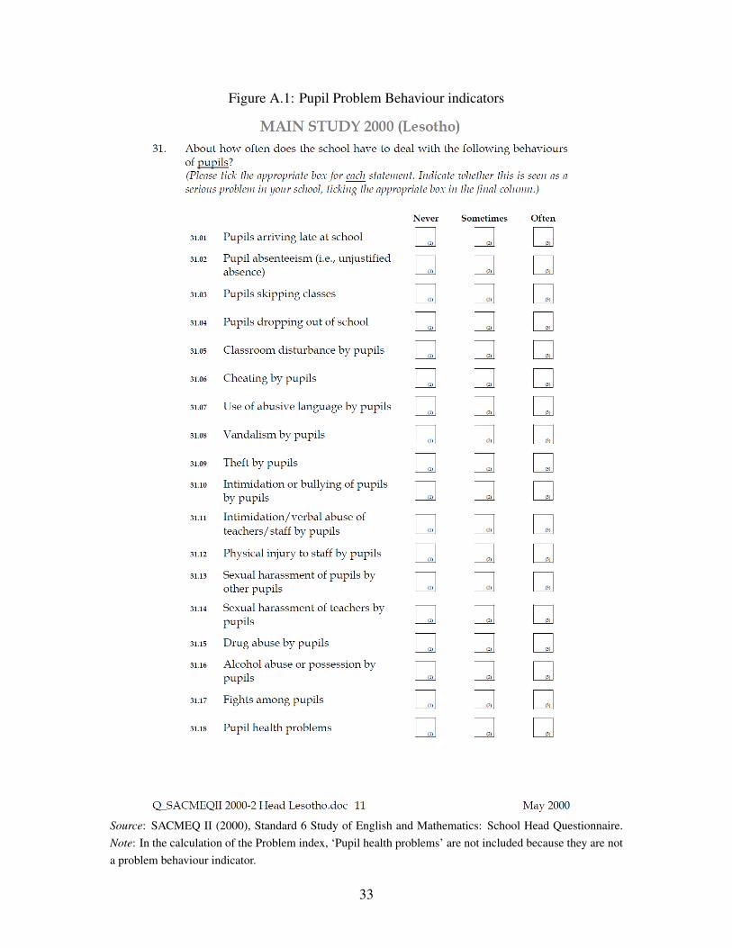
Figure A.1: Pupil Problem Behaviour indicators

Source: SACMEQ II (2000), Standard 6 Study of English and Mathematics: School Head Questionnaire.Note: In the calculation of the Problem index, ‘Pupil health problems’ are not included because they are nota problem behaviour indicator.

33

Figure A.2: Teacher Problem Behaviour indicators

Source: SACMEQ II (2000), Standard 6 Study of English and Mathematics: School Head Questionnaire.Note: In the calculation of the Teacher index, ‘Teacher health problems’ are not included because they arenot a problem behaviour indicator.

34