AVERAGE BALANCE EQUATIONS FOR GRANULAR …maeresearch.ucsd.edu/goddard/Pisa/Lecture01/Reprints/babic97.pdf · AVERAGE BALANCE EQUATIONS FOR ... the interstitial gas plays a minor

Pergamon Int. J. Engng Sci. Vol. 35, No. 5, pp. 523-548, 1997

(~) 1997 Elsevier Science Ltd. All rights reserved P l h S0020-7225(96)00094-8 Printed in Great Britain

0020-7225/97 $17.00 + 0.00

AVERAGE BALANCE EQUATIONS FOR GRANULAR MATERIALS

MARIJAN BABIC Department of Civil Engineering and Geological Sciences, University of Notre Dame, Notre Dame,

IN 46556-0767, U.S.A.

A b s t r a c t - - A general weighted space- t ime averaging procedure is developed and utilized to obtain the average balance equations for granular materials. The method is applicable to both solid-like (quasi-static) and fluid-like (granular flow) modes of granular material behavior. The average balance equations take the same mathematical form while all average quantities involved in these equations retain the same clear physical meaning whether or not the continuum hypothesis is satisfied. If it is, the average variables are continuous and smooth functions of space and time and are independent of the averaging length and time scales. Otherwise, the average variables may be discontinuous and scale-dependent, but the same average balance equations hold within the framework of calculus of generalized functions. The results include explicit expressions which can be used for calculation of the average quantities involved in the theory in terms of the microscopic 'observables' that may be available from the discrete element simulations. © 1997 Elsevier Science Ltd.

1. I N T R O D U C T I O N

1.1 Background

The mechanics of granular materials is of fundamental interest to the fields of soil mechanics, powder technology and bulk solid transport. Granular materials are two-phase systems composed of the solid phase, which consists of discrete solid particles, and the fluid phase, which fills the interstitial space between the solid particles. In many situations involving dry, coarse particulate solids, the interstitial gas plays a minor role in the mechanics of the material and can be neglected.

The most striking property of granular materials is that they can behave either as a solid or as a fluid. The solid-like ('quasi-static') mode of granular material behavior is characterized by high bulk densities and low shear rates. The stresses are generated primarily by forces between particles at points of sustained contact. The fluid-like ('rapid flow') mode of granular material behavior is characterized by moderately high bulk densities and high shear rates. The stresses are generated primarily by transfer of momentum in interparticle collisions and transfer of momentum induced by fluctuating motion of the particles.

The quasi-static regime has been studied extensively in the context of soil mechanics [1-3]. Unlike fluids, densely packed granular materials can sustain a certain amount of shear stress. As the shear stress is increased, the material eventually yields by shearing on planes where the ratio of the shear stress to the normal stress exceeds the frictional limit. The initial deformation is strongly dependent on the initial state of compaction. During the initial failure, soils can experience dilation or compaction depending on the initial state. However, if shearing motion is maintained the material tends to settle to a fairly constant volume at which it can undergo a steady shear flow. The generated stresses are independent of the rate of deformation. The most widely used initial failure criterion is Coulomb's empirical yield criterion, which stipulates a linear relationship between the shear and normal stresses on the failure plane. The constitutive theories for the rate-independent deformation of granular materials can be divided into two main classes. The first class of theories is kinematic in nature and is based on Coulomb's hypothesis or its generalization. Examples of theories of this type include the single-shearing model [4] and the double-sliding free rotating model [5, 6]. The second class of theories is based on the plasticity theory (e.g. [2, 7]). At present, there is insufficient experimental

523

IJES 35:5-D

524 M. BABIC

evidence on which to base a choice between the kinematic theories and the plasticity theories. The formulation of the appropriate constitutive theory for the solid-like behavior of granular materials is still an open question and none of the theories which have been proposed is capable of describing all observed phenomena [3].

The pioneering work on the rapid flow of granular materials is considered to be Bagnold's [8] experimental study of rapidly sheared dense granular suspensions. He observed that at high solids volume fractions both normal and shear stresses are proportional to the square of the applied shear rate. He identified the principal stress-generating mechanism in this regime to be the transfer of momentum in interparticle collisions. At lower bulk densities and lower shear rates the effects of the interstitial fluid become important and the mixture behaves as a Newtonian fluid. The effective viscosity of such a mixture is a function of the solids volume fraction. However, for rapidly sheared dry granular materials, the quadratic dependence of the stresses on the shear rate persists at all bulk densities. This behavior has been confirmed in numerous shear-cell experiments of both wet and dry mixtures [9-11].

Rapid flows of particulate materials result in vigorous random motion of individual grains which is analogous to thermal agitation of molecules in a dense gas. One significant difference between molecular and granular systems is that granular particles are inelastic and frictional, resulting in continuous conversion of the pseudo-thermal energy (i.e. kinetic energy of the fluctuating motion) into the true thermal energy (i.e. heat). Kinetic theories of rapid granular flows [12-20] extend the Chapman-Enskog kinetic theory of dense gases to account for the conversion of the pseudo-thermal energy into heat (i.e. energy dissipation) due to inelastic and/or frictional collisions. These theories are based on the following assumptions: (i) the number of particles in a macroscopically small volume is very large; (ii) the particles interact through instantaneous binary collisions; (iii) the pre-collisional velocities of colliding particles are uncorrelated ('molecular chaos' assumption); and (iv) the perturbation of the single-particle distribution function from its equilibrium Maxwellian form is small. The validity of assumption (i), which is equivalent to the continuum hypothesis, is open to discussion [21]. Assumption (ii) can be somewhat relaxed in the sense that the particle interactions need not be instantaneous, but they do have to be sufficiently brief so that simultaneous multiple interactions are highly unlikely. This assumption is required in order to formulate the balance equation for the single-particle distribution function ftJ~ involving only the two-particle distribution function f(2) and not higher order many-body distribution functions. Taking the moments of the balance equation for f~l~ yields the macroscopic balance laws for the macroscopic field variables such as the mean density, velocity, and kinetic energy density of fluctuating motion (granular temperature). This procedure also provides integral expressions for the macroscopic fluxes of momenta and energy in terms of f t~ and f~2). Assumption (iii) provides a closure hypothesis for ft21 in terms o f f t~. Finally, assumption (iv) is used to determine an approximate form of ftl~ in terms of the mean variables and their gradients. Once f~l~ is known, the constitutive equations for the macroscopic fluxes of momenta and energy, as well as the rate of energy dissipation, are found by tedious but straightforward integrations. The resulting system of equations resembles the hydrodynamic equations for a Newtonian fluid, except that the viscosity and pseudo- thermal conductivity coefficients are not material constants but depend on the fluctuation energy which is regarded as an independent field variable. The simplest version of the kinetic theory, summarized in [17], is applicable only to smooth, slightly inelastic particles. Theories [15, 16] are applicable to slightly inelastic, slightly frictional particles. More complex theories have also been developed for very dissipative smooth particles [18], very frictional particles [19], and particles that are eroded in collisions [20].

The kinetic theory appears to be successful in modeling the special flow regime for which it is intended. However, there are many engineering applications in which one or more of the restrictive assumptions upon which the kinetic theory is based is poorly if at all satisfied [22]. In particular, as the concentration increases the assumption of molecular chaos is likely to

Average balance equations for granular materials 525

break down as the particles repeatedly collide with a small set of their neighbors. As the concentration further increases, the assumption of binary collisions breaks down as the particles come into enduring, frictional contacts for extended periods of time. In some important engineering problems, such as the flow on an inclined chute, both collisional (rate-dependent) and frictional (rate-independent) mechanisms may be important [23]. One or the other of these mechanisms may be dominant at a particular inclination angle or a particular mass flow rate, but sometimes both of these mechanisms may be present in the same flow. Even though the separate theories for the limiting quasi-static and rapid flow regimes are quite advanced, they are based on very disparate foundations and a common theoretical approach is difficult to envision. The only attempts to include both mechanisms in the same theory [23-25] are based on a combination of the results from the analyses of the quasi-static and rapid flow regimes described above. The complete stress tensor is modeled as the sum of a collisional contribution, assumed to be given by the kinetic theory, and a frictional contribution, assumed to be given by the Mohr-Coulomb quasi-static theory.

An alternative approach for analysis of dry granular materials is based on a numerical solution of Newton's equations of motion for all discrete particles in a granular assembly. The discrete element method (DEM) was originally developed by Cundall [26] for rock mechanics problems and then extended by Cundall and Strack [27] to granular media such as sands. Because of its dynamic nature, this model is applicable to the entire range of granular material behavior (i.e. both fluid-like and solid-like). The method assumes that the particles are rigid except in the vicinity of contact points which are compliant (soft-particle model). An interparticle interaction model (force-displacement law) is assumed or derived from contact mechanics. In [27] a simple linear viscoelastic contact model is used. More realistic contact models have also been implemented [28]. The soft-particle models are quite inefficient for simulations of rapid flows at low particle concentrations due to the fact that an extremely large number of time steps is needed to resolve intercollisional trajectories (the time step is a function of material properties of the particles and is independent of the time scale of the flow). The hard-particle model of Campbell [29-34] is more efficient in such situations. The hard-particle simulations proceed in variable time steps between successive collisions in the system. The particles are assumed to be rigid and instantaneous interparticle collisions are resolved employing the principles of impact dynamics.

The DEM has been used extensively for fundamental studies concerning the quasi-static regime as well as the rapid flow regime (see reviews in [35, 36]). Most of the simulations have been carried out with a relatively small number of particles in 'control volumes' with artificial (usually periodic) boundaries. One of the fundamental applications of the DEM is to extract the average quantities corresponding to the macroscopic field variables that appear in the continuum-mechanical or statistical-mechanical models. However, an averaging procedure appropriate for the general case has not been systematically developed. In the DEM studies concerned with the quasi-static regime, the inertial terms are neglected in the development of relationships between the macroscopic and microscopic variables. The expression for the average stress tensor in terms of the interparticle forces has been derived by many workers [37-41]. Similar results are obtained either by an application of the principle of virtual work (e.g. [38]) or the method of volume averaging (e.g. [40, 41]). Average couple stresses are discussed in a study of statics of spherical particles by Jenkins [42].

The method of volume averaging proceeds as follows:

1 1 ~ ]

where "r is the volume-averaged stress tensor, V is the averaging volume, T is the microscopic stress field, V p is the volume of particle p, x is the position vector within particle p, and superscript T denotes tensor transpose. The summation over p E V extends over all particles

526 M. BABIC

which are wholly or partially contained in V. Note the quasi-static assumption that the stresses within the particle are in equilibrium (xV.T = 0). Application of the Gauss ' theorem results in a conversion of the volume integral over V p into the surface integral. However , for particles that are intersected by the boundary of V, this surface integral involves integrals of the stress traction over the surface area of the 'cut ' . In order to avoid this difficulty, an assumption is made that the averaging volume V may be slightly modified such that particles whose centroid is within V are considered to be wholly contained in the modified volume V' and vice versa.

Hence,

1 ! X.p xp,,fp., _- y. X (-" - (2)

V p Js; V p q -7 . q>p

where u p = 1 if the centroid of particle p is located within V and u p = 0 otherwise, S p is the surface area of particle p , n is the outward unit normal on the surface of particle p , x pq is the position vector of the contact point between particles p and q, and fPq is the resultant force exerted by particle q on particle p. The summations over p and q extend over all particles in the entire assembly with a provision that fPq = 0 if particles p and q are not in contact. The summation over p and then over q > p extends over all pairs of particles in the entire assembly, counting each pair of particles only once. If the centroids of both particles p and q are located within V , u p - u q = 0, and the contribution of such contacts to I" vanishes. The final result is effectively the sum over all contacts across the boundary of V'. Alternatively, as in [41], one may substitute x pq = X p + t pq, where x p is the position vector of the centroid of particle p and r pq is the position vector of the contact point with respect to the centroid of particle p. Equation (2) becomes:

1 Z u p Z r p q f p q 1 Z Z ( uprpq - uqrqP) fpq. ~, = 1 Z u p x p Z fpq + = (3) g p q V p q v p q>p

Note again the quasi-static assumption ~qfPq ---- O. If the centroids of both particles p and q are located within V , uPr pq - - l l q r qp- - (,,I _ rqp - - I p q where I pq is the branch vector connecting the

centroids of particles p and q. It may be argued that as the size of V increases the contribution of the boundary contacts in (3) becomes less and less significant and that 1" may be approximated by an expression of the form:

1 = -~ Y~ Z u""r ' " fP" , (4)

p q>p

where I.l pq may be defined in several ways, e.g. (i) lg pq = (U p + t/q)/2; (ii) u pq = 1 if x pq E V and u pq = 0 otherwise; (iii) IA pq = 1 if (x p + xq)/2 E V and u m = 0 otherwise; (iv) u pq is the fraction of the length of F 'q contained in V, etc. For identical circular particles definition (i) reproduces (3) exactly. Presumably, the additional approximation contained in (4) is of the same order of magnitude as the approximation of V by V'. Note that if the system is periodic and V is the unit periodic cell, u p = u q = u pq = 1 for all pairs of particles in the periodic cell. Expressions such as (2), (3) or (4) have been used to calculate the macroscopic stress tensor in virtually all quasi-static D E M applications. Due to the assumptions of static equilibrium of stresses within each particle, and static equilibrium of contact forces acting on each particle, it is not clear that these results are applicable to the rapid flow regime.

In the simulations of rapid granular flows, the macroscopic stresses are determined by a combination of volume and time averaging. In their simulations of simple shear flows of disks and spheres Walton and Braun [43, 44] calculated the average stresses from the following expression:

q£ = ~ - Zm~ , "~ ,P + lPqf pq ( t ' ) d t ' , (5) P P q >p


where ~P = v p - l ) .x p is the fluctuating velocity of particle p with respect to the mean velocity, I) = 5,e~e: is the imposed mean velocity gradient tensor, ~ is the shear rate, N is the total number of particles in an unit periodic cell, V is the volume of the unit periodic cell, m is the particle mass, t' is the time and T is the duration of the time averaging interval. Neither a derivation nor a reference concerning equation (5) were provided in [43, 44]. Babic et al. [45] derived the energy balance equation for the simple shear flow in terms of the microscopic quantities and verified that the rate of work done by the contact forces in the unit periodic cell equals T:D with I" given by (5), and thus verified that equation (5) is applicable to the simple shear rapid granular flow.

The averaging procedure used by Zhang and Campbell [46] and Campbell [33, 34] to extract distributions of stresses and couple stresses in wall-bounded flows of identical disks is summarized below. The averaging area is taken to be a strip of width equal to one particle diameter D and length equal to the width of the periodic cell L. The following averaging operations are defined:

lf0 ~ = ~ ~(uPrnqJP)(t ' )dt ' (6) P

l 0T [ XI/] =- ~ E E (ttPqttlPq)(t ') d t ' (7) p q>p

where V = L D is the area of the averaging strip, T is the duration of the time averaging • interval, m is the particle mass, ¢ is an arbitrary single-particle property (e.g. velocity), qJ is an

arbitrary property of a pair of particles in contact (e.g. an outer product of the branch vector and the contact force), u p = 1 if xP(t ') E V and u p = 0 otherwise, and u pq is taken to be the fraction of the length of the branch vector I pq that resides within V at time t'. The mean density t~ is obtained from (6) for CP= 1. The expressions for the average stress tensor "F and the average couple stress tensor M used by these authors may be written as:

T = - j6~ + [If] = - ~uPm~P~ p + ~ ~ uPqlPqf pq (t ' )dt ' P P q>P

(8)

- 1;o E ] = - Kt3~,~ + [Ira] = - E blp|~zp~p + E E UPqIPq( rpq × fPq) (t ' )dt ' P P q>p

(9)

where ~ - - v - ~7 is the fluctuation velocity of a particle with respect to the mean velocity ~, K = I / m , I is the particle moment of inertia, ~ = w - # is the fluctuation angular velocity of a particle with respect to the mean angular velocity # , ! is the branch vector, f is the contact force acting on a particle, r is the 'moment arm' vector pointing from the center of the particle to the contact point, and m = r × f is the moment of the contact force acting on a particle about the center of that particle. Zhang and Campbell [46] explained their expressions for the collisional terms as follows: "in a time step h, every collision causes a transport of momentum fh a distance 2R in the k direction" and, analogously, "in a time step h, every collision causes a transport of angular momentum mh a distance 2R in the k direction". Here R is the particle radius and k = l/(2R) is the unit vector in the direction of !. The arguments quoted above do not provide an adequate justification for equations (8) and (9). It needs to be shown that the collisional parts of T and 1~I are the apparent macroscopic collisional fluxes of the macroscopic linear momentum/5~ and the macroscopic angular momentum/SK#, respectively. It is shown in the present study that the apparent macroscopic collisional flux of the macroscopic angular momentum is zero for identical circular particles. This result is consistent with the kinetic theory of Lun [16] but obviously invalidates equation (9) used in [46] and its rigid-particle counterpart used in [33, 34].

528 M. BABIC

The problem of thermal conduction through a densely packed stationary granular material has been studied by Batchelor and O'Brien [47]. Their expression for the mean heat flux ~! E can be written as

q~ = --V1 Zu ,ZxP~lOpc = v1 ~p q>t,Z uPqlPqO pq, (10)

where QPq is the heat flux from particle q to particle p. The arguments leading to (10) are similar to those used in the derivation of equation (4) for the average stress tensor. In the rapid flow limit, the primary heat transport mechanism is the fluctuating motion of the particles [48-50]. The collisional heat transfer is relatively small because of the short duration of the collision time and the small contact area.

In spite of their prominent roles in the rapid granular flow theories, expressions for calculation of fluxes and sinks of the kinetic energy of fluctuating motion from the DEM simulations are not available in the published literature, and no data on these quantities has been reported to date.

1.2 Outline of the present study

The existing theories for the quasi-static and rapid flow regimes are based on disparate foundations. The common underlying concept is that the macroscopic field variables corres- pond to averages of the appropriate microscopic quantities. However, the averaging procedures employed in the granular materials literature in the past are restricted either to the quasi-static regime (by neglecting the inertial terms in the microscopic balance equations) or the rapid flow regime (by assuming binary collisions between the particles). On the other hand, there is a large body of literature which deals with the development of macroscopic balance equations for multiphase systems (see, for example [51-54] and references therein). Generally speaking, the results of these theories are applicable to granular materials which belong to the more general class of multiphase systems. However, simplifications offered by the particulate nature of the solid phase are not exploited. Consequently, application of these more general results to obtain relationships between the average quantities involved in the theory and the microscopic 'observables' (e.g. particle velocities, interparticle forces, etc.) that may be available from the DEM simulations is not straightforward. For example, some difficulties encountered in an application of the results from [52, 53] are as follows: (i) the expressions for the average fluxes of momenta and energy involve unknown distributions of the microscopic fluxes of momenta and energy at the intersections of the particles and the surface of the averaging volume; (ii) the angular momentum due to rotation of the particles cannot be separated from the sum of moments of linear momenta of the particles; (iii) the balance of the kinetic energy of the fluctuating particle motion cannot be considered separately from the balance of the intrinsic energy of the particles.

In the present study, the particulate nature of the solid phase is explicitly recognized in the development of macroscopic balance equations for granular materials. A general averaging procedure that is applicable to the entire range of granular material behavior is developed. The results include explicit expressions which can be used for calculation of the average quantities involved in the theory in terms of the microscopic 'observables' that may be available from the discrete element simulations.

In Section 2 the microscopic partial differential equations of mass, linear momentum, angular momentum and energy conservation are integrated over the volume of a single particle. This procedure results in a system of ordinary differential equations for particle mass, translational velocity, angular velocity, and energy. Additional balance equations for the particle translational energy, rotational energy, and intrinsic energy (which are redundant from the microscopic point of view) are developed by manipulations of the four basic conservation


equations. The entropy inequality for a single particle is also developed. The balance equations for a single particle are cast into a common form (general particle balance equation) which involves four terms: (i) the time derivative of a certain particle property; (ii) the net input of this property into the particle resulting from interparticle interactions; (iii) the net input of this property into the particle resulting from the interstitial fluid effects; and (iv) the net input of this property into the particle resulting from external effects.

In Section 3 a weighted space-time (WST) averaging technique is developed and applied to the general single particle balance equation. The weighting function w is a function of space and time whose integral over the entire space and time domains is equal to 1. A particular choice for the weighting function yields the regular volume-time averaging procedure. The general averaged balance equation valid at point x and time t is obtained as follows. The general particle balance equation written for particle p at time t' is multiplied by the weighting factor w(x p - x, t' - t) (according to the relative position of the particle centroid x p with respect to the point under consideration, and according to the time lag between the time for which the particle equation is written and the time under consideration). The results are summed over all particles in the system and then integrated with respect to t' over the entire time domain. The resulting equation is mathematically manipulated into a partial differential equation in which the independent variables are x and t. This equation states that the convective rate of change of a certain average property is equal to the sum of fluxes of this property due to the fluctuating motion and interparticle contacts plus the sum of sources of this property due to the interparticle contacts, interstitial fluid, and external effects.

In Section 4 the macroscopic balance equations for mass, linear momentum, angular momentum, translational kinetic energy, rotational kinetic energy and intrinsic energy are developed from the general macroscopic balance equation. The entropy inequality is also developed for future use in the development of constitutive equations. The average quantities which appear in the macroscopic balance equations are explicitly related to the microscopic variables such as the particle velocities, interparticle forces, etc. These relationships can be used for calculation of the macroscopic properties from the soft-particle DEM simulations.

In Section 5 the macroscopic balance equation for the intrinsic energy is manipulated into the macroscopic equation of heat conduction in order to correctly evaluate the macroscopic heat flux.

In Section 6 the results of the present theory are reduced to forms appropriate to the rapid granular flow regime. The results of this reduction can be used for calculation of the macroscopic properties from the hard-particle DEM simulations. A comparison with the balance equations developed in the kinetic theory for rapid granular flows is also performed.

Section 7 contains the discussion and conclusions of the present study.

2. BALANCE EQUATIONS FOR A SINGLE PARTICLE

The first step in derivation of the macroscopic balance equations for granular materials is integration of the microscopic balance equations over the volume of a single particle. These microscopic balance equations are the differential forms of the conservation laws for mass, linear momentum, angular momentum and energy and the entropy inequality [55]:

a,(p) + V.(pv) = 0 (11)

a,(pv) + V.(pvv) = V.T + pg (12)

at(px x v) + V.(px x vv) = V.(x x T) + px x g (13)

at(p(e + v2/2)) + V.(p(e + v2/2)v) = V.(T.v + q) + p(g-v + h) (14)

Ot(prl) + V.(pr/v) - V.s + pb. (15)

530 M. BABIC

In the above equations t is the time, d, = a/at, p is the mass density, v is the velocity, T is the

stress tensor, g is the body force per unit mass, x is the position vector of the point under

consideration, E is the internal energy density, q is the heat flux, h is the heat source per unit

mass, n is the entropy density, s is the entropy flux, and b is the entropy source per unit mass.

For simple thermomechanical processes s = q/O and b = h/B, where 8 is the thermodynamic

temperature.

Integration of equations (ll)-(14) over the volume of particle p yields

$mp, =o (16)

3 mPvp) = C fpci + fpf + mpg n

(17)

$ [m”(xP x VP + wP.KP)] = c(xp X fp4 + mp”) + xp X fPf + mp’ + mPxP X g 4

(18)

&P + i (@.v~> + +.Kp.+)] + kl’) = c (WPY + Qpq) + Wpf + Qpf + mP(g.vP + h) (19) Y

z (mP$) > ~SJ”J + Spt + ml’b”. 1,

In the above equations m” = J”,,pdu is the mass of particle p, mPvp = J”,,pvdu is the linear

momentum of particle p, 4 is the absolute linear velocity of particle p, fpq = J,,.,n.Tda is the

resultant force exerted by particle q on particle p, ALJy IS the contact area between particles p

and q, n is the outward unit normal vector on the surface of particle p, fPf = J,,>m.Tda is the

resultant force exerted by the interstitial fluid on particle p, Apt is the surface area of particle p

in contact with the interstitial fluid, mPwP.KP = JVpPr X vdu is the angular momentum of

particle p with respect to the centroid of particle p, r = x - xP is the position vector of a point

within particle p with respect to the centroid of particle p, wp is the absolute angular velocity of

particle p, mpKp = jv12p(r X I X r)du is the moment of inertia tensor of particle p, I is the

identity tensor, rnpq = J-,,,a.(r X T)da is the resultant moment exerted by particle q about the

centroid of particle p, rn”l = J,,,,, n. (r X T)da is the resultant moment exerted by the interstitial

fluid about the centroid of particle p, mPt?’ = J,,,,pedu is the total intrinsic energy of particle p,

k” = JV,>p[(v - v’ - w” X r)2/2]du is the difference between the total kinetic energy of particle p

and the kinetic energy of the rigid body motion of particle p, W”’ = J,,,JBn.T*vda is the rate of

mechanical work done by particle q on particle p, Q”” = Jn,JC,n.qda is the rate of heat transfer

from particle q to particle p, WI” = _f,,,,,n.T.vda is the rate of mechanical work done by the

interstitial fluid on particle p, Qpt = J,,,,,n.qda is the rate of heat transfer from the interstitial

fluid to particle p, m”$’ = J,,,,Pvd u is the total entropy of particle p, S”” = JA,,,,n.sda is the

entropy flux from particle q to particle p, S”’ = _fn,,r nsdu is the entropy flux from the interstitial

fluid to particle p, and m/b” = JV,,pbdu is the rate of entropy supply into particle p. The

summation over 4 extends over all particles in the system with a convention that if particles p

and q are not in contact A”” = 0 and hence f”“, ml’“, Wpq, Q”” and S’” are all zero.

In the present study, as well as in the soft-particle discrete element models, the particles are

considered to be rigid while the contacts are considered to be deformable. This statement

means that deformations are small and confined to small neighborhoods of the contact surfaces

with other particles. The velocity field within particle p is approximately equal to v =

v” + r X w” except in these small neighborhoods. The kinetic energy of the difference between

the actual velocity field and the rigid-body motion velocity field is neglected, i.e. k” = 0. The

surfaces of particles in contact are assumed to be non-conforming. In this case rn’” = rpr’ x f”“,

where rpq = xpq - xp is the position vector of the centroid of contact area AtJq with respect to


x2 X p

rqP

RPq

rPq

\

\ , \

~ . t ~ XI

0 (a) (b)

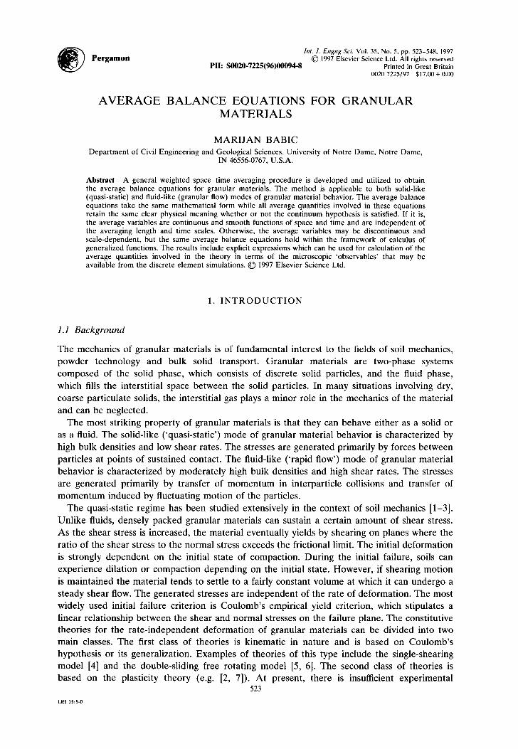
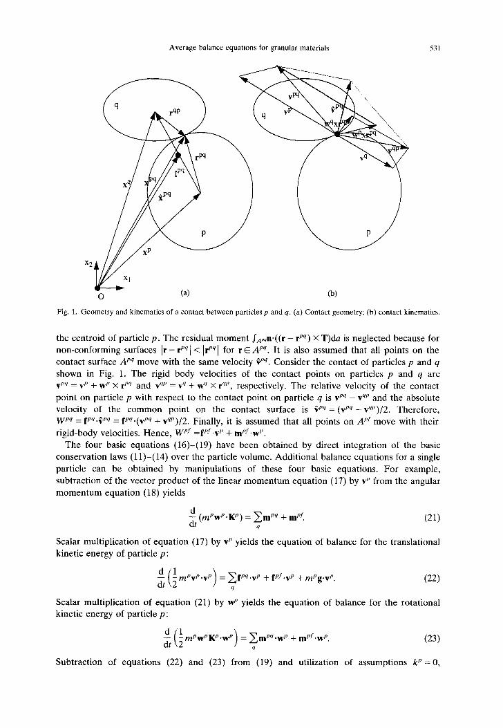
Fig. 1. Geometry and kinematics of a contact between particles p and q. (a) Contact geometry: (b) contact kinematics.

the centroid of particle p. The residual moment fA,,,n'((r - r pq) × T)da is neglected because for non-conforming surfaces I r - rPq[ ( I r P " I for r ~ z " q . It is also assumed that all points on the contact surface A pq move with the same velocity ¢,Pq. Consider the contact of particles p and q shown in Fig. 1. The rigid body velocities of the contact points on particles p and q are V pq = V p + W p X r pq and v qp = V q -~ W q X r qp, respectively. The relative velocity of the contact point on particle p with respect to the contact point on particle q is v pq - v qp and the absolute velocity of the common point on the contact surface is ¢¢Pq = ( v pq + v q P ) / 2 . Therefore, W pq = fPq'vPq = f P q ' ( v pq + VqP)/2. Finally, it is assumed that all points on A p r move with their rigid-body velocities. Hence, W ~r =fP:.v p + mP:.w p.

The four basic equations (16)-(19) have been obtained by direct integration of the basic conservation laws (11)-(14) over the particle volume. Additional balance equations for a single particle can be obtained by manipulations of these four basic equations. For example, subtraction of the vector product of the linear momentum equation (17) by v p from the angular momentum equation (18) yields

d ( m P w P ' K p) = Z m pq -4- m p:. (21) q

Scalar multiplication of equation (17) by v p yields the equation of balance for the translational kinetic energy of particle p"

dt m P Y P "Vp = f P f "Vp q

Scalar multiplication of equation (21) by w p yields the equation of balance for the rotational kinetic energy of particle p:

d ( ~ m P w P K P . w P ) = ~ m P q . w P + m P : . w P . (23) dt q

Subtraction of equations (22) and (23) from (19) and utilization of assumptions k p =0 ,

532 M. BABIC

W pq = fPq 'VPq, m pq ---- r pq X fPq and W pl = fpl.v p + mer.w p yields the equation of balance for the intrinsic energy of particle p:

d dt (meet') = E[QPq + fPq'(vPq - - vpq)] + Q~r + m P h . (24)

q

The balance of equations for a single particle developed above can be written in the following common form:

d Elffklpq + I~Pf d--t (mP~OP) = + mPf p, (25) q

where ~0 p is an integral particle property, LIJPq is the net input of this property into particle p from its (possible) contact with particle q, qJPf is the net input of this property due to the interstitial fluid and fP is the net input of this property into particle p due to external effects. The appropriate choices for lit p, YJPq, 14[Pt and fP from which equations (16), (17) and (20)-(24) can be recovered are listed in Table 1.

3. G E N E R A L A V E R A G E D B A L A N C E E Q U A T I O N

3.1 Weighting function

The weighted space-t ime average of an arbitrary function ~ is defined as:

(¢)(x,t) = x, t ' - t)dx'dt', (26)

where the integrations are carried out over the entire spatial and temporal domains, dx' is an infinitesimal volume element, dt' is an infinitesimal time increment, and w ( x ' - x , t ' - t ) is the weighting function subject to:

f f w(x' - x,t' - t)dx'dt' = l (27)

for every x and t. The weighting function vanishes as x / - * + ~ and t' -* + ~. The weighted space- t ime averaging is a very general procedure which includes many

commonly used special averaging techniques. An important special case may be obtained with:

3

w(x' - x,t' - t) = h(t' - t;ao,bo) H h ( x i ' - xi;ai,bi), (28) i--I

where / /~+a'~ ~ - a

h ( ~ ; a , b ) = C l e r f ~ ) - e r f ( ~ ) ) , (29)

and C=l/ f+~h(~;a,b)d~. In the limit b - * 0 , h(~C; a,b) tends to the step function, i.e. h ( ~ ; a , b ~ O ) - * ( 1 / 2 a ) [ U ( ~ + a ) - U ( ~ : - a ) ] , where U(~:) is the Heaviside unit step function. Hence, in the limit bi--*0 (i = 0, 1, 2, 3), the weighting function given by (28) corresponds to the volume average over a rectilinear averaging volume of dimensions (2a~, 2a2, 2a3) centered at (x~, x2, x3) and a time average over a time interval 2a0 centered at time t. In the limit a - * 0 and b - * 0 , h(sC; a, b) tends to the Dirac delta function, i.e. h(~; a - * 0 , b - * 0 ) - * 6(~). Hence, an instantaneous spatial average can be obtained with ao-* 0, while a local time average can be obtained with ai--o0 ( i = 1 , 2, 3). In the present study w ( x ' - x , t ' - t ) is regarded as a continuous and differentiable function of its spatial and temporal arguments. This restriction does not exclude the special cases mentioned above since the generalized functions involved in these averaging procedures can be viewed as the limiting forms of continuous and differentiable functions.


0

&

&

0

e~

+

+

] +

8 + a

E ~

+

&

"~ +

-~ ~I ~

. + + ~

+ o

%

+ ~ ~

o ~ . + + ~

~v w

I

+

E

534 M. B A B I C

3.2 W e i g h t e d average o f the genera l s ingle par t ic le balance equa t ion

In the spirit of (26), the contribution of the general particle balance equation (25) (written for particle p at time t') to the general macroscopic balance equation (valid at point x and time t) is weighted according to the distance between the particle centroid x p and point x and according to the time lag between times t' and t. Hence, equation (25) written for time t' is multiplied by w(x p - x, t ' - t ) , the resulting equations are summed over all particles and integrated with respect to t' over the entire time domain. The resulting equation, which involves only x and t as independent variables, is

f f\ ~ w ( x p - x , t ' - t) [mP~P( t ' ) ]d t ' = ~ w ( x p - x , t ' - t ) ~ t t l P q ( t ' ) d t ' - ~ p P q

+ f ~ w ( x P - x , t ' - t)tt~Pf ( t ' )d t ' P

( ~ ~w(x ; ' - x,t' - t ) m P f P ( t ' ) d t '. (30) + P

Note that in this manner the system of discrete solid particles has been effectively replaced by a system of discrete mass points located at the particle centroids. The contribution of particle p to the general average balance equation has been weighed as if the entire mass of particle p were concentrated at point xP(t ') at time t'. Alternatively, one could multiply the conservation laws (11)-(15) written for point x' and time t' by w ( x ' - x , t ' - t ) and integrate the resulting equations with respect to x' and t' over the entire spatial and temporal domains. It is shown in the Appendix that this alternative approach is not adequate for the present purpose because the average quantities involved in the average balance equations cannot be determined without the knowledge of microscopic distributions of p, v, T, e, and q within each particle.

3.3 Transpor t t e rms

Let A denote the left-hand side of (30). Integration by parts of this term yields

A = - f ~ ~p mPqJP(t') ~t, [w(xP - x , t ' - t)]dt ' . (31)

Since x p ~- xP(t'), application of the chain rule of differentiation yields

Z f \ ~ m P t p P ( t ' ) [ O w ( x t ~ ( ~ ' ~ - t ) O w ( x P - x ' t ' - t ) d ~ d ' ~ ( t f ' ) ] = - + dt'. (32) ;, ( - ~ ~ ( x p - x )

Note that d x P ( t ' ) / d t ' =vP(t ' ) . The partial differentiation with respect to t ' - t can be accomplished in two ways: (i) changing t' while holding t constant, or (ii) changing t while holding t' constant. These two procedures are related by:

Ow(x p - x , t ' - t) = Ow(x p - x , t ' - t) = _ Ow(x p - x , t ' - t) (33)

8(t' - t) Ot' , Ot ,,

Similarly,

Ow(x p - x , t ' - t ) _ _ Ow(x p - x,t' - t) ," (34) ~ ( x ~ - x ) ~ x

since holding t' constant is equivalent to holding x p constant. Since mPq, p and v p do not depend either on t or on x, one obtains:

0 A = ~ [ f _ ~ ~pwPmP~OP( t ' )d t ' ]+ V. [f[~ ~,wPmt ' t~PvP( t ' )d t ' ] , (35)

where w e =- w ( x p - x, t ' - t) and V is the spatial gradient with respect to x.

Average balance equations for granular materials

The average mass density t3 is defined as

Zwpm,'dC P

The mass-weighted average d] of a particle p roper ty ~b is defined by

f i~ = f ~ ~ w P ( m P q J P ) ( t ' ) dt'" P

In part icular, the mass-weighted velocity ~ is defined by

Hence , A can be expressed as

where

535

(36)

(37)

fi~' = ~ w P ( m P v P ) ( t ' ) d t '. (38) p

A = ~ (fi~b) + V . ( f i # ) - 7.FK(~b),

f ~c

FK(~b) = _ ~wP(mp~bp~p) ( t ' ) d t '.

(39)

(40)

He re ~P = v p = ~ is the fluctuation velocity of particle p with respect to the mass-averaged velocity.

3.4 Interpart icle interact ion terms

Let B deno te the first t e rm on the r ight-hand side of (30). Symmetr iza t ion of this te rm with respect to particles p and q yields

B = I S ~ ~ [ I ~ J P q w ( x P - - x , t ' - t ) + Y J q P w ( x q - x , t ' - t ) ] d t ' . (41) p q > p

This t e rm can be split into two parts, i.e. as B = B l + B2, where

B1 = ~ ~ ( W pq + w q P ) ( w ( x p - x , t ' - t) + w ( x q - x , t ' - t ) )dt ' (42) q > p

B2 = ~ ~ ~ (W pq - ~qP)(w(x p - x , t ' - t) - w(xq - x , t ' - t))dt ' . (43) zc p qZ>p

In t roducing a d u m m y variable s, B 2 can be expressed as follows:

Bz = ~ -~ Z ( Wqp - weq) ~ [w( xp + sipq - x , t ' - t)] dsdt ' . (44) q > p

Util izat ion of the chain rule in the derivative with respect to s yields

if[ (, B2 = 5 ~-' ~ (ttmP - tppq) lpq. [w(x p + sip q - x , t ' - t)]dsdt ' . (45) zc p q > p ,tO

Using (33) in (45) finally yields:

B2 = V. ~ (u2 eq - ~ " e ) F " w(x r + sl p`, - x , t ' - t )]dsdt ' . (46) q > p

536 M. BABIC

Therefore,

where

B = SC(O) + V.FC(O), (47)

sc(~ 9) = f~ ~ Z (qtpq + q3qp)w~qdt' (48) p q>p

] ff~ ~p Z IPq( qlpq --qlqp)wp~qdt, FC(O) = ~ q>p (49)

f0 1

w p-q = w(x p + sl pq - x , t ' - t )ds (50)

1 W pq = ~ [W(X p -- X,t' - t) + W(X q - X,t' - t)]. (51)

In the above calculation the interaction term B has been split into a source term SC(~O) and a flux term FC(0). These two terms involve averaging of (wPq + WqP) and F q ( w p q - ~qP),

respectively. It is very important to note that the weighting coefficients WPF q and wPs q are in general different from each other. Consider, for example, the simplest case of the vo lume- t ime averaging for which the weighting function is given by (28) and (29) with bi = 0 (i = 0, 1, 2, 3). In this case w~L~ q = ( V T ) -1 if centroids of both particles p and q are located within the averaging volume V at time t ' , w pq= ( 1 / 2 ) ( V T ) -~ if only one of these centroids is located within V at t '

and w!~ q= 0 if neither of these centroids is located within V at t ' . On the other hand, w p-q is equal to ( V T ) ~ times the fraction of the length of [Pq contained in V at time t ' . Hence, w((. q= w pfl = ( V T ) ~ if both centroids and the entire branch vector are inside of V at t ' ,

"q = w p," = 0 if neither of the centroids nor any portion of the branch vector are inside of V W S

at t ' , but w~ q ~ w pq otherwise. If V is relatively large compared to the characteristic particle size this difference is not expected to significantly affect the average quantities because the difference affects only contacts near the boundaries of the averaging volume. The average quantities calculated correctly, i.e. with contributions to the flux terms weighted by w p~I and contributions to the source terms weighted by w pq, would probably be similar to the corresponding quantities in which the contributions to the flux and source terms would both be

,,,P'/ However , if V is relatively small the differences between w p~ and w(~, q weighted with w~ -q or ~ s • are extremely important.

3.5 The f ina l result

Substitution of (39) and (47) into (30) yields the general averaged balance equation:

3 (/~t~) + V-(t3t~) = V.[FK(0) + FC(0)] + SO(O) + ~f(qJ) + s F ( o ) ,

where

sF(qo = ~wpqsef( t ' )d t'

~ f ( O ) = F ~p W"mPfP( t ' )d t ' .

(52)

(53)

The general average balance equation takes the same form whether or not the continuum hypothesis is satisfied. If it is, the average variables are continuous and smooth functions of space and time and are independent of the averaging length and time scales. Otherwise, the average variables may be discontinuous and/or scale-dependent, but the same average balance equations hold within the f ramework of calculus of generalized functions. If the weighting

(54)


function is smooth and continuous the average variables are smooth and continuous as well but may be scale-dependent. If the weighting function is a generalized function (e.g. volume-t ime average) the average variables are discontinuous. If the continuum hypothesis is satisfied the discontinuities are infinitesimal. Otherwise, they are finite but may be relatively small.

In any case, the average balance equations take the same mathematical form and the average variables involved in these equations have the same clear physical meaning. The physical meaning of various average quantities will be revealed in the next section.

4. M A C R O S C O P I C B A L A N C E E Q U A T I O N S

The macroscopic balance equations for mass, linear momentum, angular momentum, translational kinetic energy, rotational kinetic energy, intrinsic energy and entropy are obtained by substitution of the appropriate choices for qJP, W 'q, W p' and fP into equations (37), (40), (48), (49), (53) and (54) to obtain, respectively, ~, FK(qJ), SC(tp), ~,c, SF(q0 and f(~0). This procedure is summarized in Table 1 and the final results are stated below:

• conservation of mass

a,(~) + v - ( ~ ) = 0 (55)

• conservation of linear momentum

0,(/~) + (~3~,~) = v . ' r + fig + t r (56)

• balance of angular momentum

0,(/5~.R) + V.(f3~,@.R) = V-I~I + m c + m F (57)

• balance of translational energy

0 ,D(e T + U ) ] + v . D ( e T + U ) q = v-( t- ,7 + ~ ) + ~g-~ - z ~ + ¢ . ~ + D ~ ' (58)

• balance of rotational energy

o,[~(e R + ER)] + V.[~(e R + ~ ) ~ 1 = V . ( ~ . ~ + ~ ) - z '~ + m ~ . ~ + 1) ' ~ (59)

• balance of intrinsic energy

O,(~g) + V . ( ~ ) = V.~ E + ~h + z r + z R + QF (60)

• entropy inequality

a , ( ~ ) + v . ( ~ ) _> v-~ + ~t; + s ~. (61)

In the above equations "r = T K + T c is the stress tensor, t F is the rate of supply of linear momentum to the particles by the interstitial fluid, @.K is the internal spin density, 1~I = MK+ M c is the couple stress tensor, m F is the rate of supply of internal spin to the particles due to interparticle contacts, m F is the rate of supply of internal spin to the particles by the interstitial fluid, E r = ({.~)/2 is the kinetic energy density of the mean translational motion, e r is the kinetic energy density of the fluctuating translational motion, ~r = q~v + qrC is the flux of kinetic energy of the fluctuating translational motion, z r is the rate of conversion of the translational kinetic energy into other forms of energy, DrF is the rate of supply of the kinetic energy of the fluctuating translational motion to the particles by the interstitial fluid, E R = (@.K.@)/2 is the kinetic energy density of the mean rotational motion, e R is the kinetic energy density of the fluctuating rotational motion, ~n = qnK + qRC is the flux of kinetic energy of the fluctuating rotational motion, z R is the rate of conversion of the rotational kinetic energy into other forms of energy, D RF is the rate of supply of the kinetic energy of the fluctuating rotational motion to the particles by the interstitial fluid, ~*" = qEK + R~:C is the flux of the mean intrinsic energy, QF is the rate of supply of the intrinsic energy to the particles by the

538 M. BABIC

interstitial fluid, ~ = s K + s c is the flux of mean entropy and S F is the rate of entropy supply to the particles by the interstitial fluid.

The flux terms consist of a transport contribution (with superscript K) and a contact contribution (with superscript C). The transport and contact contributions to the stress tensor are:

T K = - f ~ Z w P m P v v d t ' (62) P

T c = f ~ ~p ,,>p~ wPqlPqfPqdt '. (63)

The internal spin density ~,-K is defined via

~¢v'~, = f ~ ~wPmPwP.KPdt ' (64) P

#K = f~ ~wPmPKPdt'. (65) P

The transport and contact contributions to the couple stress tensor are

M K = - wPmPv pw p 'K pdt' (66)

if M e`= ~ ~ ~ WPFqlPq(m pq - mqP)dt '. (67) p q > P

Note that for identical circular particles nl pq = m qp and therefore M c = 0. This result invalidates equation (9) used in [33, 34, 46] and the distributions of collisional couple stresses reported therein. The structure of T c and M c is similar, but the difference in the final result occurs because fPq = - - f q P while m pq = m qp. The rate of supply of internal spin due to interparticle contacts is

m ~ = ( ~ ~ ~ ,,,Pq]Pqvv.s. >( fPqdt'. (68) d x p q > p

The kinetic energy densities of the fluctuating translational and rotational motion are given by:

fie 7., =21 f ~ ZwPmp~p.~Pdt (69)

1 f~ ~wPmP~P'KP'WPdt '. (70) =

The transport and contact contributions to the fluxes of kinetic energies of the translational and rotational fluctuating motions are

qTK = _ _1 f~ ZwPmp~p.~p~Pdl ' (71) _ ~ p

qrC = 2 ~ ~ WPF'qPqfPq'(~ "p + ~q)dt' (72) - - ~ p q > P

qm¢ = _ _1 f_~ ~wPmp(#p.Kp.~p)~dt ' (73) 2 _~ p

qRC = 2 ~'~ w¢~.qPq(m pq .~" - mqP.~'q)dt'. (74) q > p


The rates of conversion of the translational and rotational kinetic energies into other forms of energy are:

Z T = - - E E W P q r P q ' ( V p - - vq ) d t ' ( 7 5 ) - ~ p q > P

= -- I ~ E E WPq( nlpq'Wp + nlqP'wq) dt'. (76) Z g P q > p

The transport and contact contributions to the fluxes of intrinsic energy and entropy are

qEK _= -- f~_~ ~wPmPep~Pdt , (77) P

qeC = E E wPFqlPqQ p°dt' (78) --zc p q > p

S I~ = -- EwPmPrlPvPdt ' (79) p

sc = f~_~ E E WPF qlpqspqdt'' (80) p q > p

Finally, the fluid-solid interaction terms are given by

t F = f~_~ ~ w P f P l d t ' (81) P

m F = f_~ E w P m P f d t ' (82) P

DTF = f ~ ~wpfpI .~Odt, (83) P

f D RF = E w p m pf .wPdt' (84)

QF = ~ w p Q p f d t , (85)

S F = wPSPfdt '. (86)

5. E Q U A T I O N OF H E A T C O N D U C T I O N

In this section the average balance equation for the intrinsic energy is developed into the heat conduction equation. This procedure has two purposes: (i) to determine the macroscopic heat flux (~E is the macroscopic flux of the intrinsic energy, not heat), and (ii) to determine the rate of mechanical energy dissipation into heat (z r + zn is the rate of conversion of the kinetic energy into the intrinsic energy, not heat). The intrinsic energy consists of the heat energy and the strain energy associated with elastic deformations of particles in contact.

The total intrinsic energy me p of particle p is decomposed into a thermal contribution mPCPO p = fv,,pCPOdv and a strain energy contribution q~P= fv,,(T~::E/2)dv. Here C p is the heat capacity of particle p, 0 p is the average temperature of particle p, T E is the elastic part of

540 M. BABIC

the stress tensor and E is the strain tensor. For small strains E = [Vu + (Vu)r]/2, where u is the

displacement vector. Hence,

1 fv,(TE:Vu)dv, 2 1 ( ( + , . : = . , , : . <,,-, .u> v - .,,

For small displacements, the second term on the right-hand side of (87) can be neglected. Utilization of the Gauss ' theorem in the first term yields

~b" = ~ n'T"+"udv = ~ b "q, (88) aSP q

where 05 pq = ( f~q.~ 'q) /2 , fPq = f s , ,n .TEdv is the elastic part of the contact force and u pq is the average displacement of material points on the surface of particle p in contact with particle q. By definition, an incremental change of the strain energy &h pq induced by an incremental displacement 611 pq is ~ P q = fPq'~u pq. Hence, the rate of change of the strain energy can be expressed as 05 vq = fPq.6fi pq, where ff'q is the average displacement rate of material points on the surface of particle p in contact with particle q. This displacement rate can be expressed as fiPq = ~?Pq - - V P q , where v v+' = v v + w p X r pq and ~Pq = (v pq + vqP)/2. Hence

d~b pq - f f ~ " ' ( ~ " ' - v"q). ( 8 9 )

dr '

Substitution of the decomposit ion mPeP = mPCPO p + ~,qch pq into the intrinsic energy balance

equation yields

a ~ ~wPchPUdt, ) a,(~O) + V'(t~ ~0+)+ -ftt(f~,, /

+ V ' ( f ~ + t~ ~ ~ w P b P q v P d t ' ) + V . ~ l " + ~ h + z ' + z ~, (90)

where 0 is the average tempera ture defined via

~CO = (~ ~ w " m P C " O P ( t ' ) d t ' (91) 3 ~

P

and C' is the average heat capacity, defined as

~ C = (~ ~ ,wPmPCPdt ," (92) P

The total heat flux ~H consists of a contact part q .C = qtZC and a transport part q .K, which is given by

q.t~ = _ f ~ E m P C p O p ~ P d t , " P

(93)

The last two terms on the left-hand side of (90) can be combined as follows:

E w P ~ P q d t ' EwP~bPqvPdl ' ) "-" /Ow p . V w e ) d t , - - ~ , ¢bpq l - - +(f_++. )++.(f+++ =f+++ +: Ot _~ q - ~ ' - \ a t

= - ~ ~,c~ q--d--~-dt = w e - - d t '~- 2 . ,w"" -aS - "d t ' . (94) p q dr' q>p ~t

The total rate of conversion of the kinetic energy into the intrinsic energy z r + zR can be expressed as

z r + zR = - (~ E E wPq[ff" ' ( vpq - eeqP) + f fP'( vqp - ~qP)ldt'. (95) P q > p


The contact force ffq can be decomposed into the elastic part fPq and the dissipative part f~q. Using this decomposition and (89) in (95) yields

q>p dt dt' -]- ~ WPqfPq' (v qp -- vPq)d t ' . (96) q>p

It can be seen that z T + Z R consists of two parts. The first part represents the rate of conversion of the kinetic energy into the strain energy (which is a part of the intrinsic energy), while the second part represents the rate of conversion of the kinetic energy into heat (the rate of mechanical energy dissipation). Substitution of (96) and (94) into (90) results in cancellation of the strain energy terms. The final equation of heat conduction for granular materials becomes

Ot(fiCO) + V.(~CO~) = V'~ H 4- QF 4- fih + y,

where y is the rate of mechanical energy dissipation:

T = Z wPqfPq'( vqp -- VPq) d t ' ' q>p

(97)

6. RAPID G R A N U L A R FLOW LIMIT

In this section the results of the present theory are reduced to forms appropriate to the rapid granular flow regime.

6.1 General f o r m s o f the interaction terms f o r the rapid f l ow regime

The distinguishing feature of rapid granular flows is that the interparticle interactions are brief and binary. Under the assumption of binary and brief (but not instantaneous) collisions between the particles, the interaction terms (48) and (49) can be evaluated as follows. Suppose that particles p and q have been observed to collide N pq times during the entire time of observation. Let :q':, where c = 1,2 . . . . . N pq, denote the starting time of the cth collision between particles p and q and let T pqc denote the duration of this collision. It is assumed that T pqc is small enough that the probability of another particle colliding with the pair ( p , q ) during any of their collisions can be neglected. Furthermore, it is assumed that during the collision x p and x q remain constant. In this case the integrations over time in (48) and (49) can be replaced by sums of N pq integrations over the brief time intervals T pqc as follows:

NPq F C ( o ) = ~ 1 Z Z ZIPqC( ~Jpqc -- l~qpc) wpqc

E. p q > p c

Nl'q

= T. 2 X(O + p q>p c

where ~t pqc + Tpq c

ff~pq, = J~, . . . . q lPq( t ' ) d t '

~qc = xq(tpqc) -- xP(tpqc)

1 wE ' t '= ~ [w(xP(t pq') - x , t ' - t) + w(xq( t pq') - x , t ' - t)]

(98)

(99)

(100)

(101)

(102)

fo I WPff Ic = w ( x P ( t pqc) + s l pqc -- x , t ' - t ) d s . (103)

In order to evaluate ~1 pqc, consider the general single-particle balance equation (25) written

542 M. BABIC

at an instant during the cth collision of particles p and q. Since the collision is assumed to be binary, there are no other particles interacting with particle p at this instant and equation (25) thus becomes

d - - (m"~" ) = W I'" + W"f + mPf p. (104) dt'

Integration of this equation with respect to t' from t pqc to tPqc+ T pqc yields

~pqc = (mp~p)(tpq, + T,,,I,.) _ (mp~p)(tt, q, .) _ (mpff, + Cp1~l )Tpq, ' (105)

where t~pf is the average of qjpl during the interval T pq'. Since T pq' is small, the last term in the above equation can be neglected. Substitution of (105) into (98) and (99) yields

1 FC(~O) = ~ ~ l " ' " ( m " A 6 " q " - m " 2 ~ " ' ) w p;~' (106)

pqc

sC ( ~J) = E (mP A 6 pq' + m q A 6 " ' ) w { ~ q', (107) pqc

where the triple summations in equations (98) and (99) (which extend over all collisions observed in the system during the entire time of observation) are symbolically represented by the summations over pqc and Atp pqC = ~ P ( t pqc + T pqc) - ~ P ( t pqc) is the change in ~0 p during the cth collision between particles p and q.

6.2 Collisional terms in the macroscopic balance equations

The collisional terms in the macroscopic balance equations for the rapid granular flows are obtained by substitution of the appropriate choices for ~0 p from Table 1 into (98) and (99). The results are as follows:

TC = 1 ~lpqC(mP Avpq, - mq Avqpc)w~,c= E l l , qcjpqCwPtlC (108) 2 pqc pqc

= I P q c ( m P K P . m w P q C - m q K q . A w q p c ) W p y ' = E I p q c L pqc x J p q " w pgc (109) -- pqc pqc

m c = ~ ( m P K " . ± w P " " + mqKq.awq"DwP"" (110) pqc

1 1 , /1 \ 7 ,,, qrC _ 2 1 p q , [ m p A ( _ ~ . ~ t t q , , = 2 pq,, L \2 / - m ' l A ~ , . ~ ' ) ' " J w S [ . ' (111)

pqc

1 , 1 q n C = - ; l P q " [ m ' A ( - C v . K P . ~ ] P q c - m q A ( ~ . K q . ~ ) P q ~ ] W P F " ' (113)

2 pqc L \2 ]

Z R= - ~ [ m P A ( ~ w . K P . w ) P q C + m q A ( ~ w . K q . w ) P q ' ] w , ~ q c (114) pqc

q/-;c = ! Ewpqclpqc(mP At?pqc _ mq AFpq ,) = EwpqclpqcHpq , (115) 2 pqc pqc

sC = 21 p,,,~-" wpqqpqc (mp A npqc + m,l A rl,,,,,. ) = pq,~ w"qqPqc NP"c, (116)

where LPqc=(rPq"+rqP")/2, jpqc =mPAvPq,.= _m,JAvqm. is the force impulse exerted by


particle q on particle p during their cth collision, H pqc= mPAE pqc= --mqAg qpc and N pqc= mPAI) pqc= -mqAl) qpc are the total amounts of heat and entropy, respectively, transferred from particle q to particle p in their cth collision. Equations (108)-(114) can be used for calculation of the collisional terms from the hard-particle DEM simulations.

6.3 Comparison with the kinetic theory

In the kinetic theories for rapid granular flows which include the effects of particle rotation [15, 16], the ensemble average of the single-particle quantity q, is defined as

_ 1 I1)q,fO)(x,c,w;t)dedw, (117) n(x,t)

where f(l) is the single-particle distribution function, defined such that f¢l)(x,c,w; t)dxdcdw is the probable number of particles in a fixed volume element dx centered at x with translational velocities within de centered at e and angular velocities within dw centered at w, and n(x,t) is the local number density of the particles given by

n(x,t) = I1) fO)(x'c'w;t)dedw" (118)

Multiple integrations with respect to all components of dc and dw are denoted by "(1)". The general transport equation for the rate of change of (q,) can be expressed as [17]

O,(n(g,)) + V-(n(g,e)) = ~b c + n(g'Vcq,), (119)

where ~b c is the collisional rate of increase of the mean of q, per unit volume and V¢ is the gradient operator in the velocity space. The collisional term can be expressed as

1 I (mA~bOf(2)(x'cl'wl;x +trk , cz,wz;t)dC

1 f (mA~2)f(2)(x_ o'k, cl,wl,x, c2,w2;t)dC, (120) + 2 2)

where m is the particle mass, or is the particle diameter, Aq,1, and Aq,2 are changes of the property q, experienced by particles 1 and 2 in the collision, f(2) is the pair distribution function defined such that f<2)(xl, cl, wl; x2, c2, w2; t)dxldxzdcldc2dwldw2 is the probable number of pairs of particles such that particle 1 is located within dx~ centered at x~, has translational velocity within dCl centered at c 1 and angular velocity within dw I centered at wl while particle 2 is located within dx2 centered at x2, has translational velocity within dc2 centered at c2 and angular velocity within dw2 centered at w2. Furthermore, k = (x2-Xl) / t r is the unit vector pointing from the center of particle 1 to the center of particle 2, dC = (c~ - c2).kdkdc~dc2dw~dw~, and dk is the elementary solid angle within which k lies. Integrations indicated in (120) are carried out over all impending collisions, i.e. through full ranges of dc~, de2, dw~, dw2 and through a portion of the range of dk for which ( c l - c2)-k>0. Multiple integrations with respect to dC are denoted by "(2)".

The collisional term 4, c is next decomposed into a flux term and a source term. As shown in [17], after expanding f(2)(X- o'k, cl, wl; x, C2, W2; t) into a Taylor series the resulting flux term takes a form of a series that involves spatial derivatives of f(2)(x - ark, c~, w~; x, c2, w2; t) up to an infinite order. For slightly inelastic and slightly frictional particles, this term can be approximated by an expression that involves f(2)(X- trk/2, c~, wl; x + o-k/2, c2, w2; t) but no spatial derivatives [16]. In [18] a more compact general expression for the flux term, which involves an integral f~f(2)(x + strk - ~rk, c~, w~; x + strk, c2, w2; t)ds rather than a Taylor series, is used.

In order to facilitate comparison with the present theory, the collisional term ~b c is

544 M. BABIC

manipula ted in a slightly different but equivalent way compared to [18]. ~ c is first split into two parts as follows:

4, ( = f2)(mAq, i + mAq,2)f ~.?dC + ~ f2)(mAg, l - m Aq,2)f dC, (121)

where

12 1 fF = ~ [f(2)(X,¢l ,Wl ;X + crk,c~,w2;t) + f (2)(x - ~rk,c, ,w] ;X,C 2,w2;t)]

F = f (2) (x ,c I ,w 1 ;x + crk,c2,w2;t ) -- f~2)(X -- crk,c, ,wl ;x,c2,w2;t).

We can write F as

F = [f(2)(x + s~rk - o'k, el ,w~ ;x + s~rk, c2,w2;t)] ds

= ~rk.V (2)(x + s~rk - o-k,e~ ,w~;x + so'k,e2,w2;t)ds = V-(o'kfl.?),

Hence

where

where

£1( ) f~? = f(2) X + s~rk - ~rk, cl ,w~;x + s o ' k , c2,w2; t ds.

(122)

(123)

(124)

(125)

ch c = XC(qO + V.O c, (126)

ZC(~J) = f(2)(mA~0' + mAOz)f~?dC (127)

1 f 6rk(mA~l _ mA~z)fJ~2dC. (128) -0((~[t) • 2 2)

The above decomposi t ion of the collisional te rm into a source term Zc($) and a flux term _0c0p) is equivalent to the decomposi t ion in [18], which does not require that the particles be slightly inelastic and slightly frictional as in [16].

Subst i tut ion of (126) into (119) yields the general t ransport equation:

O,(n(tp)) + V.(n(~0)(e)) = V.[_0K(~0) + 0c(t0)] + Z((~b) + n(g.V,,~0) (129)

where _ ~ ( ~ ) = -n ($~ ' ) is the t ransport flux of n ($) and ~ = c - ( c ) is the fluctuation particle velocity with respect to the mean. By taking $ to be the particle mass m, linear m o m e n t u m me, angular m o m e n t u m Iw, translat ional kinetic energy mc2/2, and rota t ional kinetic energy Iw2/2, the following balance equat ions are obtained:

o,(~) + v . ( ~ ) = o (13o)

o , ( p ~ ) + v . ( ~ ) = v . ~ + p g (131)

b,(/~KW) + V- ( / fK~) = V.]~! + m c (132)

3,[t~(e T + fi2/2)] + V.[t~(e 7 + ~2/2)~] = V.(I".~ + ~r) +/~g.~ _ z ' (133)

O,[/~(e n + Kff212)] + V'[t3 (e n + K~v2/2)~] = V.(i~l.~ + 4 ~) - z ~, (134)


where t~ = mn, ~ = (c), # = (w), e r = (t~2)/2, e R = K(ff2)/2, K = I / m , t = T K + T c, 1~1 = M r +

M C, ~ = q~" + q~C, q" = q " " + q"~ , T " = - p ( ~ , T ~ = _~ (m ~) , M K = - ~ K ( ~ ) , M ~ =

_0~(I~), m c = Z ( I * ) , q r , , = _ ~ ( e : ~ / 2 , qTC = _0C(me2/2), qR,, = _ ~ K ( ~ 2 ~ / 2 , qR~ = _0,: i(~2/2),

z T = - z C ( m c 2 / 2 ) , and z R= - z C ( I w 2 / 2 ) . Compared with [16], the equations have the same form but there are differences in the form of collisional flux and source terms due to the approximation in the collisional term ~b c adopted in [16]. One difference is that m ci ~ eijkT~k.c

The system of equations (130)-(134) is sufficient to describe the mechanics of slightly inelastic, slightly frictional particles. More advanced/less restrictive theories, e.g. Refs [18, 19], require additional balance equations which can be easily developed from the general transport equation (125).

Comparison of equations (130)-(134) with (55)-(59) indicates that the balance equations of the kinetic theory have the same form as the more general balance equations developed in the present theory. Comparison of the single-particle average quantities indicates that iS, v, w, e T, e k, T K, M K, qrK, and qRK a re identical in both theories provided that t ~ = (mn~b), i.e.

f~ ~, ~bPwP dt' = fl )tbf° )(x,c, w;t )dcdw. (135) P

Comparison of the flux terms indicates that T c, M c, qrC, qnC are identical provided that

~lPqc( m~llpqc - m~lPqC)wPq : I I(A~bl - A~b2)f~dC. (136) pqc 2)

Comparison of the source terms indicates that m c, z T and z R are identical provided that

~'~(A0Pqc + AtPPqC)wPsq = I (AOl + A~bz)f~ZdC. (137) pqc 2)

Note similarities between WPF q and f}2 as well as between WPs q and fPq. Equations (135), (136) and (137) explicitly relate the probabilistic averages involved in the

kinetic theory to the weighted space-time averages involved in the present work. The question of whether these two types of averages are equal is related to the ergodicity hypothesis of statistical mechanics [56]. Let {P} denote an ensemble formed from all particles observed in the averaging volume during the averaging time interval. If the ensemble {P} contains sufficient information from which the single-particle distribution function can be accurately constructed, the two averaging procedures in (135) will give identical results. Let {C} denote the ensemble of all collisions observed in the averaging volume during the averaging interval. If the ensemble {C} contains sufficient information from which the pair-distribution function at the point of contact can be accurately constructed, the two averaging procedures in (136) and (137) will also give identical results.

7. D I S C U S S I O N A N D C O N C L U S I O N S

A general weighted space-time (WST) averaging procedure is developed and utilized to obtain the average balance equations for granular materials. The procedure is applicable to both solid-like (quasi-static) and fluid-like (rapid granular flow) modes of granular material behavior. The results are valid for an assembly of particles of arbitrary sizes and shapes. The description of the system includes the average balance equations for mass, linear momentum, angular momentum, translational kinetic energy, rotational kinetic energy, intrinsic energy and entropy (55)-(59). The effects of the interstitial fluid are included. Explicit expressions which

546 M. BABIC

can be used for calculation of the average quantities involved in these balance equations in terms of the microscopic 'observables' that may be available from the discrete element simulations are given by (30), (32) and (62)-(86). These results are subject to the following approximations and restrictions:

1. The system of discrete solid particles has been effectively replaced by a system of discrete mass points located at the particle centroids. This replacement has occurred in equation (30) where the contribution of each particle to the general average balance equation has been weighed according to the relative position of the particle centroid with respect to the point under consideration. The error involved in this approximation is at present unknown. An alternative approach is pursued in the Appendix, but it is shown that this approach does not yield the required expressions for calculation of the average quantities involved in the resulting balance equations in terms of the microscopic 'observables ~. Furthermore, the present theory is fully compatible with the kinetic theory for rapid granular flows, which is also based on the mass-point approach.

2. The results are not valid in vicinity of physical boundaries of the system. The results are valid only for points x such that w(x' - x, t' - t) is small or zero for any x' within a layer of thickness [r[ m~× along any of the physical boundaries. Here [r[ ..... is the largest possible distance from a particle centroid to its surface (among all particles in the system). Suppose, for illustration, that the weighting function is given by (28) with b,--~ 0 and that the physical boundary is a flat wall located at x3 ~ x~' with an inward normal in the x3 direction. The results of the present theory are valid only for points x such that x3 > x ~ + a3 + [r I .... . This restriction is necessary so that particles whose centroids are located within the averaging volume centered at x cannot possibly interact with the physical boundary at any time. Similar restrictions must be placed for all boundaries in the system. An extension of the present theory to include the part icle-boundary interactions is planned.

3. The dependence of the weighting function on its spatial and temporal arguments is the same for every x and t (i.e. the weighting function does not depend explicitly on x or t). If the weighting function is given by (28) with bi--~ 0, this restriction means that the size and orientation of the averaging volume must be the same at all points of space. An extension of the present theory to account for variations of the weighting function with respect to space and time is planned. These variations may yield additional terms in the average balance equations caused solely by the gradients of the weighting function. This extension would allow a DEM 'experimentalist ' to divide a complex domain into suitable arbitrary subvolumes (similar to finite elements) and extract the correct averages of interest corresponding to each subvolume.

In regard to the existing expressions for the average stress tensor, it is shown that equations (4) and (8) are justified provided that u p~ in these equations is taken to be the fraction of the length of the branch vector I pq that resides within V. The present theory invalidates equation (9) for the average couple stress tensor used in Refs. [33, 34, 46]. The macroscopic heat flux reduces to equation (10) when the particles are not in motion.

New expressions for fluxes and sources of kinetic energies of translational and rotational fluctuating motions are obtained. It is shown that the flux terms and source terms should be weighed differently (by w~ -q and wP't). This distinction is very important when the averaging length scale is comparable to the characteristic particle size.

The present theory is fully compatible with the kinetic theory for rapid granular flows. For a consistent correspondence it is important to keep the distinction between ,,,m~VVF and w(~ q (in the averaging theory) as well as to use the exact decomposition of the collisional integral into the flux and source terms (in the kinetic theory).

The results of the present study have an immediate application to calculations of the average quantities from the DEM simulations (both soft-particle and hard-particle). They also may


provide a foundation for future development of a general thermomechanical theory for granular materials.

R E F E R E N C E S

1. Sokolovskii, V. V., Statics o f Granular Media. Pergamon Press, Oxford, 1965. 2. Schofield, A. N. and Wroth, C. P., Critical State Soil Mechanics. McGraw-Hill, New York, 1968. 3. Spencer, A. J. M., in Mechanics o f Solids, Rodney Hill 60th Anniversary Volume, ed. H. G. Hopkins and J. J.

Sewell. Pergamon, Oxford, 1981. 4. Mandl, G. & Fernandez-Luque, R., Geotechnique, 20 (1970) 277-307. 5. Spencer, A. J. M., J. Mech. Phys. Solids, 12 (1964) 337-351. 6. De Josselin De Jong, G., Geotechnique, 21 (1971) 155-163. 7. Drucker, D. C. & Prager, W., Q. AppL Math., 10 (1952) 157-165. 8. Bagnold, R. A., Proc. Roy. Soc. Lond., A225 (1954) 49-63. 9. Savage, S. B. & Sayed, M., J. Fluid Mech., 142 (1984) 391-430.

10. Hanes, D. M. & Inman, D. L., J. Fluid Mech., 150 (1985) 357-380. 11. Craig, K., Buckholtz, R. H. & Domoto, G., J. Appl. Mech., 53 (1987) 935-942. 12. Jenkins, J. T. & Savage, S. B., J. Fluid Mech., 130 (1983) 187-202. 13. Lun, C. K. K., Savage, S. B., Jeffrey, D. J. & Chepurney, N., J. Fluid Mech., 140 (1984) 223-256. 14. Jenkins, J. T. & Richman, M. W., Arch. Rat. Mech. Anal., 87 (1985) 355-377. 15. Lun, C. K. K. & Savage, S. B., J. Appl. Mech., 54 (1987) 47-53. 16. Lun, C. K. K., J. Fluid Mech., 233 (1991) 539-559. 17. Savage, S. B., in Continuum Mechanics in Environmental Sciences and Geophysics, ed. K. Hurter. Springer-Verlag,

New York, 1993. 18. Jenkins, J. T. & Richman, M. W., J. Fluid Mech., 192 (1988) 313-328. 19. Nakagawa, M., Kinetic Theory for Plane Flow of Rough, Inelastic, Circular Disks. Ph.D. Dissertation, Cornell

University, Ithaca, NY, 1988. 20. Richman, M. W. & Chou, C. S., J. Appl. Math. Phys. (ZAMP), 40 (1989) 883-898. 21. Haft, P. K., J. Fluid Mech., 134 (1983) 401-430. 22. Haft, P. K., in Granular Matter, ed. A. Mehta. Springer-Verlag, New York, 1994. 23. Johnson, P. C., Nott, P. & Jackson, R., J. Fhdd Mech., 210 (1990) 501-535. 24. Savage, S. B., in Proceedings o f U.S.-Japan Seminar on New Models and Constitutive Relations in the Mechanics of

Granular Materials, ed. J. T. Jenkins and M. Satake. Elsevier, Amsterdam, 1982. 25. Johnson, P. C. & Jackson, R., J. Fhdd Mech., 176 (1987) 67-93. 26. Cundall, P. A., in Proc. Symp. Int. Soc. Rock. Mech. Nancy, 1971. 27. Cundall, P. A. & Strack, O. D. L., Geotechniqae, 29 (1979) 47-65. 28. Dobry, R. and Ng, T.-T., in Proceedings o f 1st U.S. Conference on Discrete Element Methods, ed. G. G. W.

Mustoe, M. Henriksen and H. P. Huttelmaier. Golden, CO, 1989. 29. Campbell, C. S. & Brennen, C. E., J. Fluid Mech., 151 (1985) 167-188. 30. Campbell, C. S. & Brennen, C. E., J. Appl. Mech., 52 (1985) 172-178. 31. Campbell, C. S. & Gong, A., J. Fhdd Mech., 164 (1986) 107-125. 32. Campbell, C. S., J. Fhdd Mech., 203 (1989) 449-473. 33. Campbell, C. S., J. Fluid Mech., 247 (1993) 111-136. 34. Campbell, C. S., J. Fluid Mech., 247 (1993) 137-156. 35. Cundall, P. A. and Hart, R. D., in Proceedings o f 1st U.S. Conference on Discrete Element Methods, ed. G. G. W.

Mustoe, M. Henriksen and H. P. Huttelmaier. Golden, CO, 1989. 36. Campbell, C. S., Ann. Rev. Fhdd Mech., 22 (1990) 57-92. 37. Drescher, A. & De Josselin De Jong, G., J. Mech. Phys. Solids, 20 (1972) 337-351. 38. Christofferson, J., Mehrabadi, M. M. & Nemat-Nasser, S., J. Appl. Mech., 48 (1981) 339-344. 39. L. Rothenburg, L. and Selvadurai, A. P. S., in Mechanics o f Structured Media, Part B, ed. A. P. S. Selvadurai.

Elsevier, Amsterdam, 1981, p. 469. 40. Cundall, P. A., Drescher, A. and Strack, O. D. L., in Proceedings o f IUTAM Conference on Deformation and

Failure of Granular Materials. Delft, 1982, p. 355. 41. Cundall, P. A. and Strack, O. D. L., in Mechanics of Granular Materials: New Models and Constitutive Equations,

ed. J. T. Jenkins and M. Satake. Elsevier, Amsterdam, 1983, p. 137. 42. Jenkins, J. T., in Modern Theory o f Anisotropic Elasticity and Applications, ed. J. Wu, T. C. T. Ting and M.

Barnett. SIAM, Philadelphia, 1991, p.368. 43. Walton, O. R. & Braun, R. L., J. Rheology, 30 (1985) 949-980. 44. Walton, O. R. & Braun, R. L., Acta Mechanica, 63 (1987) 73-86. 45. Babic, M., Shen, H. H. & Shen, H. T., J. Fhdd Mech., 219 (1990) 81-118. 46. Zhang, Y. & Campbell, C. S., J. Fhdd Mech., 237 (1992) 541-568. 47. Batchelor, G. K. & O'Brien, R. W., Proc. Roy. Soc. Lond., A355 (1977) 313-333. 48. Wang, D. G. & Campbell. C. S., J. Fhdd Mech., 244 (1992) 527-546. 49. Louge, M. Y., Yusof, J. M. & Jenkins, J. T., J. Heat and Mass Transfer, 36 (1993) 265-275. 50. Hsiau, S. S. & Hunt, M. L., J. Heat Transfer, I15 (1993) 541-548. 51. Drew, D. A., Ann. Rev. Fhdd Mech., 15 (1983) 261-291. 52. Hassanizadeh, M. & Gray, W. G., Adv. Water Res., 2 (1979) 131-144. 53. Hassanizadeh, M. & Gray, W. G., Adv. Water Res., 2 (1979) 191-203. 54. Ahmadi, G. & Ma, D., Int. J. Multiphase Flow, 16 (1990) 323-340.

548 M. BABIC

55. Eringen, A. C., Mechanics of Continua. Robert E. Krieger, Malabar, FL, 1967. 56. Cercignani, C., The Boltzmann Equation and its Applications. Springer-Verlag, New York, 1988.

(Received 24 October 1994; accepted 31 July 1996)

A P P E N D I X

In this appendix the WST method is applied directly to a typical microscopic conservation equation. Equations (11)-(13) can be written for point x' and time t' in the following common form:

0, (pq,) + vx,.(pq, v) = vx..J(~,) + p f ( 0 ) , ( A . l )

where a,, denotes the temporal derivative with respect to t', V x, is the spatial gradient with respect to x'~ ~b -= l, v, x × v, e + v2/2, $(q,) --- 0, T, x × T, T.v + q, f(~0) ~ 0, g, x × g, g-v + h. For simplicity a dry granular material is considered, i.e. the interstitial fluid is ignored. Multiplication of equation (A.1) by w(x' - x, t' - t) followed by integrations with respect to x' and t' over the entire spatial and temporal domains yields the following average conservation equation for the particulate phase:

a , ( ~ ) + Vx.(t3t}~7) - V~.( - ¢3~ + j(~0)) + t3f(0), (A.2)

where a, denotes the temporal derivative with respect to t, V~ is the spatial gradient with respect to x, and

/3 = f ~'~ f w ( x ' - x , t ' - t ) p ( x ' , t ) d x ' d t ' (A.3) a T p a V P

t)dxd, (a.4,

Equations (A.2) and (52) have the same form but the average quantities are defined differently. Equation (A.2) can be regarded as exact if the particles are considered to be full-bodied while equation (52) is exact if the particles are considered to be mass points. Unfortunately, no further progress is possible with equations (A.2)-(A.5) unless the microscopic distributions of p, q~ and J within the particles are known. In practice, these distributions are unlikely to be available. On the other hand, positions of particle centroids, linear and angular particle velocities, and interparticle forces and moments may be available from the DEM simulations. In order to relate the average quantities to these microscopic 'observables' either the mass-point approach must be adopted or an approximation must be made in equations (A.2)-(A.5). If an assumption is made that w(x' x, t ' - t) ~ w(x;' - x, t ' - t), one obtains

fi = ( ~'~wt'mPdt' (A.6) a T p

= ( 1 . 7 3

](tb) = [ ~]wt'Jt'dt ', (A.8) a T p

where m P ~ p = f v p ( p l ] t ) ( x ' t t ' ) d x ' and ,F' = fw, J(x't')dx'. Note that ~ and ~ are now defined in the same way as in the mass-point approach, but J (0) and FC(q,) are different. It is not clear if there is any advantage in this approach over the mass-point approach used in the present study. The contribution of each particle to the average quantities is in both cases weighted according to the relative position of the particle centroid with respect to the point under consideration. On the other hand, there are several disadvantages of the above approach compared to the mass-point approach. First, it is not possible to evaluate JP except if V.I = 0 everywhere within each particle. In this case JP = fgt, V.(xJ)dv' = Y~qxoq,I ;'q. For example, in this way one can obtain the expressions (2) for the quasi-static average stress tensor and (10) for the average heat flux, but these results are not necessarily valid for the general case when the particles are in motion. Second, the averaging procedure outlined above is applicable only to the conservation equations for mass, linear momentum, angular momentum and energy. It would be difficult to obtain separate balance equations for the mean angular velocity and the mean kinetic energies of translational and rotational motions. As shown in the present study, all desired results are obtained easily using the mass-point approach.

Documents

AVERAGE BALANCE EQUATIONS FOR GRANULAR …maeresearch.ucsd.edu/goddard/Pisa/Lecture01/Reprints/babic97.pdf · AVERAGE BALANCE EQUATIONS FOR ... the interstitial gas plays a minor