Averting Catastrophes: The Strange Economicsof Scylla and Charybdis

Ian W. R. Martin Robert S. Pindyck∗

This draft: June 5, 2014

Abstract: How should we evaluate public policies or projects to avert, or reduce the likeli-

hood of, a catastrophic event? Examples might include inspection and surveillance programs

to avert nuclear terrorism, investments in vaccine technologies to help respond to a “mega-

virus,” or the construction of levees to avert major flooding. A policy to avert a particular

catastrophe considered in isolation might be evaluated in a cost-benefit framework. But be-

cause society faces multiple potential catastrophes, simple cost-benefit analysis breaks down:

Even if the benefit of averting each one exceeds the cost, we should not necessarily avert all

of them. We explore the policy interdependence of catastrophic events, and show that con-

sidering these events in isolation can lead to policies that are far from optimal. We develop

a rule for determining which events should be averted and which should not.

JEL Classification Numbers: Q5, Q54, D81

Keywords: Catastrophes, catastrophic events, willingness to pay, policy objectives, climate

change, pandemics, nuclear terrorism.

∗Martin: London School of Economics, London, UK. Pindyck: Sloan School of Management, MIT, Cam-bridge, MA. Our thanks to Robert Barro, Simon Dietz, Christian Gollier, Derek Lemoine, Bob Litterman,Deborah Lucas, Antony Millner, Gita Rao, Edward Schlee, V. Kerry Smith, Nicholas Stern and seminar par-ticipants at LSE, Harvard, MIT, the University of Arizona and ASU for helpful comments and suggestions.

1

“ ‘Is there no way,’ said I, ‘of escaping Charybdis, and at the same time keepingScylla off when she is trying to harm my men?’

“ ‘You dare-devil,’ replied the goddess, ‘you are always wanting to fight somebodyor something; you will not let yourself be beaten even by the immortals.’ ”

Homer, Odyssey, Book XII, trans. Samuel Butler.

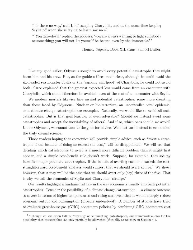
Like any good sailor, Odysseus sought to avoid every potential catastrophe that might

harm him and his crew. But, as the goddess Circe made clear, although he could avoid the

six-headed sea monster Scylla or the “sucking whirlpool” of Charybdis, he could not avoid

both. Circe explained that the greatest expected loss would come from an encounter with

Charybdis, which should therefore be avoided, even at the cost of an encounter with Scylla.

We modern mortals likewise face myriad potential catastrophes, some more daunting

than those faced by Odysseus. Nuclear or bio-terrorism, an uncontrolled viral epidemic,

or a climate change catastrophe are examples. Naturally, we would like to avoid all such

catastrophes. But is that goal feasible, or even advisable? Should we instead avoid some

catastrophes and accept the inevitability of others? And if so, which ones should we avoid?

Unlike Odysseus, we cannot turn to the gods for advice. We must turn instead to economics,

the truly dismal science.

Those readers hoping that economics will provide simple advice, such as “avert a catas-

trophe if the benefits of doing so exceed the cost,” will be disappointed. We will see that

deciding which catastrophes to avert is a much more difficult problem than it might first

appear, and a simple cost-benefit rule doesn’t work. Suppose, for example, that society

faces five major potential catastrophes. If the benefit of averting each one exceeds the cost,

straightforward cost-benefit analysis would suggest that we should avert all five.1 We show,

however, that it may well be the case that we should avert only (say) three of the five. That

is why we call the economics of Scylla and Charybdis “strange.”

Our results highlight a fundamental flaw in the way economists usually approach potential

catastrophes. Consider the possibility of a climate change catastrophe — a climate outcome

so severe in terms of higher temperatures and rising sea levels that it would sharply reduce

economic output and consumption (broadly understood). A number of studies have tried

to evaluate greenhouse gas (GHG) abatement policies by combining GHG abatement cost

1Although we will often talk of ‘averting’ or ‘eliminating’ catastrophes, our framework allows for thepossibility that catastrophes can only partially be alleviated (if at all), as we show in Section 4.1.

1

estimates with estimates of the expected benefits to society (in terms of reduced future

damages) from avoiding or reducing the likelihood of a bad outcome.2 To our knowledge,

however, all such studies look at climate change in isolation. We show that this is misleading.

A climate catastrophe is only one of a number of potential catastrophes that might occur

and cause major damage on a global scale. Other catastrophic events may be as likely or more

likely to occur, could occur much sooner, and could have an even worse impact on economic

output and even mortality. Examples include nuclear terrorism, an all-out nuclear exchange,

a mega-virus on the scale of the Spanish flu of 1918, or bioterrorism.3 One could of course

estimate the benefits to society from averting each of these other potential catastrophes, once

again taking each in isolation, and then given estimates of the cost of averting the event,

come up with a policy recommendation. But as we will show, applying cost-benefit analysis

to each event in isolation can lead to a policy that is far from optimal.

Conventional cost-benefit analysis can be applied directly to “marginal” projects, i.e.,

projects whose costs and benefits have no significant impact on the overall economy. But

policies or projects to avert major catastrophes are not marginal; their costs and benefits can

alter society’s aggregate consumption, and that is why they cannot be studied in isolation.

Like many other studies, we measure benefits in terms of “willingness to pay” (WTP), i.e.,

the maximum fraction of consumption society would be willing to sacrifice, now and for ever,

to achieve an objective. We can then address the following two questions: First, how will the

WTP for averting Catastrophe A (let’s say a climate catastrophe) change once we take into

account that other potential catastrophes B, C, D, etc., lurk in the background? We show

that the WTP to eliminate A will go up.4 The reason is that the other potential catastrophes

reduce expected future consumption, thereby increasing expected future marginal utility

before a climate catastrophe occurs. This in turn increases the benefit of avoiding the

climate catastrophe. Likewise, each individual WTP (e.g., to avert just B) will be higher

the greater is the “background risk” from the other catastrophes. What about the WTP to

avert all of the potential catastrophes? It will be less than the sum of the individual WTPs.

2Most of these studies develop “integrated assessment models” (IAMs) and use them for policy evaluation.The literature is vast, but Nordhaus (2008) and Stern (2007) are widely cited examples; other examplesinclude the many studies that attempt to estimate the social cost of carbon (SCC). For a survey of SCCestimates based on three widely used IAMs, see Greenstone, Kopits and Wolverton (2013) and InteragencyWorking Group on Social Cost of Carbon (2010). Most of these studies, however, focus on “most likely”climate outcomes, not low-probability catastrophic outcomes. See Pindyck (2013a,b) for a critique anddiscussion. One of the earliest treatments of environmental catastrophes is Cropper (1976).

3Readers with limited imaginations should read Posner (2004), who provides more examples of potentialcatastrophes and argues that society fails to take these risks seriously enough, and Sunstein (2007).

4As we will see, this result requires the coefficient of relative risk aversion to exceed one.

2

The WTPs are not additive; society would probably be unwilling to spend 60 or 80% of

GDP (and could not spend 110% of GDP) to avert all of these catastrophes.

WTP relates to the demand side of policy: it is society’s reservation price—the most it

would sacrifice—to achieve some goal. In our case, it is a measure of the benefit of averting a

particular catastrophe. It does not tell us whether averting the catastrophe makes economic

sense. For that we also need to know the cost. There are various way to characterize such

a cost, e.g., a fixed dollar amount, a time-varying stream of expenditures, etc. In order to

make comparisons with the WTP measure of benefits, we express cost as a permanent tax

on consumption at rate τ , the revenues from which would be just enough to pay for whatever

is required to avert the catastrophe.

Now suppose we know, for each major type of catastrophe, the corresponding costs and

benefits. More precisely, imagine that we are given (perhaps by some government agency) a

list (τ1, w1), (τ2, w2), . . . , (τN , wN) of costs (τi) and WTPs (wi) associated with projects to

eliminate N different potential catastrophes. That brings us to our second question: Which

of the N “projects” should we choose to implement? If wi > τi for all i, should we eliminate

all N potential catastrophes? Not necessarily. We show how to decide which projects to

choose to maximize social welfare.

When the projects are very small relative to the economy, and if there are not too many of

them, the conventional cost-benefit intuition prevails: since no project is mutually exclusive,

we should implement any project whose benefit wi exceeds its cost τi. This intuition would

apply, for example, for the construction of a dam to avert flooding in some area. Conventional

cost-benefit analysis applies to marginal projects, i.e., ones that are small relative to the

overall economy and thus have a negligible impact on total consumption.

Things are much more interesting when projects are large relative to the economy, as

might be the case for the global catastrophes mentioned above, or if they are small but

large in number (so that their influence in aggregate is large). “Large” projects change total

consumption and marginal utility, and as a result the usual intuition breaks down: There

is an essential interdependence among the projects that must be taken into account when

formulating policy. We show how to do so. We also explore several examples to illustrate

some of the more counterintuitive results that arise when determining which catastrophes

should and which should not be averted.

For instance, we consider an example in which there are three potential catastrophes.

The first has a benefit w1 much greater than the cost τ1, and the other two have benefits

greater than the costs, but not that much greater. Naive reasoning would suggest that we

should eliminate the first catastrophe and then decide whether to eliminate the other two,

3

but we show that such reasoning is wrong. If only one of the three were to be eliminated, we

should indeed choose the first; and we would do even better by eliminating all three. But

we would do best of all by eliminating the second and third and not the first: the presence

of the second and third catastrophes makes it suboptimal to eliminate the first. (On the

other hand, if the catastrophes were smaller—if all costs and benefits were divided by some

sufficiently large number—then we should eliminate all three.)

To see why some form of interdependence is inevitable, imagine that there are many

types of independent catastrophes that could in principle be averted, and that the costs

and benefits of doing so are the same for each type. Conventional cost-benefit analysis

would direct us either to avert all or none, depending on whether benefits exceed costs. But

averting all catastrophes would reduce consumption almost to zero. We show that, indeed,

the optimal policy in this stylized example is to avert some subset of the catastrophes.

In the next section we explain our basic framework of analysis by focusing on the WTP

to avert a single type of catastrophe (e.g., nuclear terrorism), taken in isolation and ignoring

other types of catastrophes. The model is simple: we use a constant relative risk aversion

(CRRA) utility function to measure the welfare accruing from a consumption stream, we

assume that the catastrophe arrives as a Poisson event with known mean arrival time, it can

occur repeatedly (we also treat the single-occurrence case, but in an appendix), and on each

occurrence it reduces consumption by a random fraction. Although it might appear that

this “single-type” model is an extension of the existing literature on generic “consumption

disasters,” it is in fact quite different.5 We examine a particular type of catastrophe and find

the WTP to eliminate it completely or reduce the likelihood of it occurring by some amount.

Most importantly, our framework allows us to treat a discrete set of catastrophes, each with

its own characteristics, show how the WTPs are related to each other, and determine the

optimal set that should be averted.

In Sections 2 and 3 we allow for multiple types of catastrophes. Each type has its own

mean arrival rate and its own impact distribution. We find the WTP to eliminate a single

type of catastrophe and show how it depends on the existence of other types, and we also find

the WTP to eliminate several of the types at once. Our first observation is that the presence

of multiple catastrophes may make it less desirable to try to mitigate some catastrophes for

5Examples of that literature include Backus, Chernov and Martin (2011), Barro and Jin (2011), Martin(2008) and Pindyck and Wang (2013). Some of these papers use more general Epstein–Weil–Zin recursivepreferences to measure welfare, which we avoid to keep things as simple as possible. Martin (2008) estimatesthe welfare cost of consumption uncertainty to be about 14%, most of which is attributable to highercumulants (disaster risk) in the consumption process. Barro (2013) examines the WTP to avoid a climatechange catastrophe with (unavoidable) generic catastrophes in the background.

4

which action would appear desirable, considered in isolation. Next, given information on

the cost of eliminating (or reducing the likelihood of) each type of catastrophe, we examine

the set of potential projects, and show how to find the welfare-maximizing combination of

projects that should be undertaken.

Section 4 discusses several extensions of our model. First, we show that our framework

allows for the partial alleviation of catastrophes, i.e., for policies that reduce the likelihood

of catastrophes occurring rather than eliminating them completely. The paper’s central in-

tuitions apply even if the policy choice is a continuous variable (i.e., even if we can adjust

the arrival rate of each catastrophe on a continuous spectrum). Second, we show that our

framework easily handles catastrophes that are directly related to one another: for exam-

ple, averting nuclear terrorism might also help avert bioterrorism. Third, we show that our

framework can handle bonanzas as well as catastrophes, that is, projects such as blue-sky

research that increase the probability of events that raise consumption (as opposed to de-

creasing the probability of events that lower consumption). Finally, we discuss catastrophes

that cause the death of some fraction of the population instead of a drop in consumption.

The contribution of this paper is largely theoretical: we provide a framework for analyzing

different types of catastrophes and deciding which ones should be included as a target of

government policy. Determining the actual likelihood of nuclear terrorism or a mega-virus,

as well as the cost of reducing the likelihood, is no easy matter. Nonetheless, we want to

show how our framework might be applied to real-world government policy formulation. To

that end, we survey the (very limited) literature for seven potential catastrophes, discuss how

one could come up with the relevant numbers, and then use our framework to determine

which of these catastrophes should or should not be averted.

1 WTP to Avoid One Type of Catastrophe

We first consider a single type of catastrophe. It might be a climate change catastrophe, a

mega-virus, or something else. What matters is that we assume for now that this particular

type of catastrophe is the only thing society is concerned about. We want to determine

society’s WTP to eliminate the possibility that this type of catastrophe will occur. By WTP

we mean the maximum fraction of consumption, now and throughout the future, that society

would sacrifice to avoid this type of catastrophe. Of course WTP could have other forms,

e.g., the maximum percentage of consumption society would give up starting at a specific

future time, or the maximum percentage of consumption over some limited time horizon.

Defining WTP as we do here is relatively simple, and consistent with most other studies.

5

It is important to stress that this WTP is a reservation price, i.e., the most society

would sacrifice. It might be the case that the revenue stream corresponding to this WTP

(and presumably collected by the government) is insufficient to eliminate the risk of the

catastrophe occurring, in which case eliminating the risk is economically infeasible. Or, the

cost of eliminating the risk might be lower than the corresponding revenue stream, in which

case the “project” would have a positive net social surplus. The WTP applies only to the

demand side of government policy. Later, when we examine multiple types of catastrophes,

we will also consider the supply (i.e., cost) side.

To calculate a WTP, we must consider whether the type of catastrophe at issue can occur

once and only once (if it occurs at all), or can occur repeatedly. For a climate catastrophe, it

might be reasonable to assume that it would occur only once—the global mean temperature,

for example, might rise much more than expected, leading to large increases in sea levels,

and causing economic damage far greater than anticipated, and perhaps becoming worse and

worse over time as the temperature keeps rising.6 But for most potential catastrophes, such

as a mega-virus, nuclear terrorism, or nuclear war, it is more reasonable to assume that the

catastrophe could occur multiple times. Throughout the paper we will assume that multiple

occurrences are indeed possible. However, in Appendix A we examine the WTP to eliminate

a particular type of catastrophe that can occur only once.

We will assume that without any catastrophe, real per-capital consumption will grow

at a constant rate g, and we normalize so that at time t = 0, C0 = 1. Let ct denote log

consumption. We define a catastrophe as an event that permanently reduces consumption

by a random fraction φ, so that if the catastrophic event first occurs at time t1, Ct = egt for

t < t1 and then falls to Ct = e−φ+gt at t = t1. For now we impose no restrictions on the

probability distribution for φ. We use a simple CRRA utility function to measure welfare,

and denote the index of relative risk aversion by η and rate of time preference by δ. We will

generally assume that η > 1, so utility is negative. The analysis is the same if η < 1, except

that utility will be positive. Later we treat the special case of η = 1, i.e., log utility.

We assume throughout this paper that the catastrophic event of interest occurs as a

Poisson arrival with mean arrival rate λ, and that the impact of the nth arrival, φn, is i.i.d.

across realizations n. Thus the process for consumption is:

ct = logCt = gt−N(t)∑n=1

φn (1)

6That is why some argue that the best way to avert a climate catastrophe is to invest now in geoengineeringtechnologies that could be used to reverse the temperature increases. See, e.g., Barrett (2008, 2009), Kouskyet al. (2009), and MacCracken (2009).

6

where N(t) is a Poisson counting process with mean arrival rate λ, so that when the nth

catastrophic event occurs, consumption is instantly multiplied by the random variable e−φn .

To simplify the analysis, we follow Martin (2013) by introducing the cumulant-generating

function (CGF),

κt(θ) ≡ logE ectθ ≡ logECθt .

As we will see, the CGF summarizes the effects of various types of risk in a very simple

way. In our case, since the process for consumption given in (1) is a Levy process, we can

simplify κt(θ) = κ(θ)t, where κ(θ) means κ1(θ). In other words, the t-period CGF scales

the 1-period CGF linearly in t. We show in the appendix that the CGF is then7

κ(θ) = gθ + λ(E e−θφ1 − 1

). (2)

Given this consumption process, and assuming CRRA utility with relative risk aversion

η 6= 1, welfare is

E∫ ∞0

1

1− ηe−δtC1−η

t dt =1

1− η

∫ ∞0

e−δteκ(1−η)t dt =1

1− η1

δ − κ(1− η), (3)

where κ(1− η) is the CGF of equation (2) with θ = 1 − η. Note that equation (3) is quite

general and applies to any distribution for the impact φ. But note also that welfare is finite

only if the integrals converge, and for this we need δ − κ(1− η) > 0 (Martin (2013)).

Eliminating the catastrophe is equivalent to setting λ = 0 in equation (2). We denote

the CGF in this case by κ(1)(θ). (This notation will prove convenient later when we allow

for several types of catastrophes.) With λ = 0 the CGF is simply

κ(1)(θ) = gθ. (4)

So if we sacrifice a fraction w of consumption to avoid the catastrophe, welfare is

(1− w)1−η

1− η1

δ − κ(1)(1− η). (5)

The WTP to eliminate the event (i.e., to make λ = 0) is the value of w that equates (3) and

(5), i.e.,1

1− η1

δ − κ(1− η)=

(1− w)1−η

1− η1

δ − κ(1)(1− η).

7We could allow for ct = gt−∑N(t)n=1 φn, where gt is any Levy process, subject to the condition that ensures

finiteness of expected utility. (For the special case in (1), gt = gt for a constant g.) This only requires thatthe term gθ in the CGFs is replaced by g(θ), where g(θ) is the CGF of g1, so if there are Brownian shockswith volatility σ, jumps with arrival rate ω and stochastic impact J , g(θ) = µθ + 1

2σ2θ2 + ω

(E eθJ − 1

).

This lets us handle Brownian shocks and unavoidable catastrophes without modifying the framework. Sincethe generalization has no effect on any of our qualitative results, we stick to the simpler formulation.

7

This representation is quite general, and will be useful below. In particular, we do not need

to assume that the consumption process is deterministic in the absence of the catastrophe.

Should society avoid this catastrophe? This is easy to answer because with only one type

of catastrophe to worry about, we can apply standard cost-benefit analysis. The benefit is

w, and the cost is the permanent tax on consumption, τ , needed to generate the revenue

to eliminate the risk. We should avoid the catastrophe as long as w > τ . As we will see

shortly, when there are multiple potential catastrophes the benefits from eliminating each

are interdependent, causing this simple logic to break down.

The CGF of (2) applies to any distribution for the impact φ. However, we will sometimes

assume for purposes of numerical examples that z = e−φ is distributed according to a power

distribution with parameter β > 0,

b(z) = βzβ−1 , 0 ≤ z ≤ 1 . (6)

In this case, E(e−φθ) = β/(β + θ). A large value of β implies a large E z and thus a small

expected impact of the event.8 Given this distribution for z, the CGF is simply

κ(θ) = gθ − λθ

β + θ. (7)

In this special case, the CGF tends to infinity as θ → −β from above. For the condition that

δ − κ(1 − η) > 0 to have any chance of holding, we must therefore assume that β > η − 1:

catastrophes cannot be too fat-tailed.

What is the WTP to avert the catastrophe? Given the power distribution for z = e−φ,

after substituting (7) and (4) for κ(1− η) and κ(1)(1− η), the WTP is

w = 1−[1− λ(η − 1)

ρ(β − η + 1)

] 1η−1

,

where ρ ≡ δ+g(η−1). We will have w < 1 as long as the parameters are such that expected

utility, with or without catastrophes, is finite. This means that we need

ρ− λ(η − 1)

β − η + 1> 0.

If this does not hold, expected utility (with catastrophes) is unbounded as t grows. This

constraint can actually be quite restrictive. If η = 2, g = δ = .02, and β = 3 (so that

8A power distribution of this sort has often been used in modeling (albeit smaller) catastrophic eventssuch as floods and hurricanes; see, e.g., Woo (1999). Barro and Jin (2011) show that the distribution providesa good fit to panel data on the sizes of major consumption contractions. Note E(z) = β/(β + 1), and thevariance of z around its mean is var(z) = β/[(β + 2)(β + 1)2].

8

E z = .75 and Eφ = .25), we need λ < .08, i.e., the event cannot on average occur more than

every 12 years. But if β = 1.5 (so that E z = .60 and Eφ = .40), we need λ < .02, i.e., the

event cannot on average occur more than every 50 years. Alternatively, if λ = .04, we need

β > 2, i.e., an event that occurs on average every 25 years cannot reduce consumption by

more than a third. And if δ = 0 (a rate of time preference that some have argued is “ethical”

for intergenerational comparisons), we would need β > 3 so E z > .75. These restrictions on

λ and/or β are reasonable for most of the catastrophic events that we might think about

(environmental catastrophes, nuclear or bio-terrorism, major earthquakes). However, once

we allow for more than one type of event, the restrictions become more severe.

2 Two Types of Catastrophes

In the previous section we have shown how to calculate the WTP to avert a single type

of catastrophe, ignoring the existence of other potential catastrophes. We now extend the

analysis to multiple types of catastrophes, show how to find the WTP to avert each type,

and then examine the interrelationship among the WTPs. We can then address the question

of how to choose which catastrophes should be averted.

In this section, we consider only two types of catastrophes. This will allow us to illustrate

some (but not all) of the key points, and is relatively simple. For simplicity, we assume that

a catastrophic event causes destruction (i.e., a drop in consumption) but not death. We also

assume that these events occur independently of each other. So log consumption is

ct = logCt = gt−N1(t)∑n=1

φ1,n −N2(t)∑n=1

φ2,n (8)

where Ni(t) is a Poisson counting process with mean arrival rate λi, and the CGF is

κ(θ) = gθ + λ1(E e−θφ1 − 1

)+ λ2

(E e−θφ2 − 1

).

Here we write φi for a representative of any of the φi,n (since catastrophic impacts are all

i.i.d. within a catastrophe type). If neither catastrophe has been eliminated, welfare is

E∫ ∞0

1

1− ηe−δtC1−η

t dt =1

1− η

∫ ∞0

e−δteκ(1−η)t dt =1

1− η1

δ − κ(1− η).

If catastrophe of type i has been eliminated, welfare is

1

1− η1

δ − κ(i)(1− η)

9

where the i superscript indicates λi has been set to zero. If both catastrophes are eliminated,

we get the same expression with κ(1,2)(1− η), which indicates that both λ1 and λ2 are zero.

Thus, willingness to pay to eliminate catastrophe i satisfies

(1− wi)1−η

1− η1

δ − κ(i)(1− η)=

1

1− η1

δ − κ(1− η)

and hence

wi = 1−(δ − κ(1− η)

δ − κ(i)(1− η)

) 1η−1

. (9)

Similarly, the WTP to eliminate both catastrophes is

w1,2 = 1−(

δ − κ(1− η)

δ − κ(1,2)(1− η)

) 1η−1

.

2.1 Interrelationship of WTPs

How is the WTP to avert Catastrophe 1 affected by the existence of Catastrophe 2? We can

think of Catastrophe 2 as a kind of “background risk” that has two effects: It (a) reduces

expected future consumption, while increasing the variance of future consumption; and (b)

thereby raises future expected marginal utility. Remember that each catastrophic event

reduces consumption by some percentage φ. The first effect therefore reduces the WTP

because there is less (future) consumption available, so that the event causes a smaller drop

in consumption. The second effect raises the WTP because the loss of utility is greater

when total consumption has been reduced. If η > 1 so that expected marginal utility

rises sufficiently when consumption falls, the second effect dominates, and the existence of

Catastrophe 2 will on net increase the benefit of averting Catastrophe 1, and raise its WTP.

This can be seen from equation (9). The CGF κ(1 − η) summarizes the effects of both

sources of risk; compared to a world in which Catastrophe 2 did not exist, it will be larger,

making w1 larger. Consider our power law example, in which zi = e−φi follows a power

distribution with parameter βi, so that

κ(1− η) = g(1− η)− λ1(1− η)

β1 − η + 1− λ2(1− η)

β2 − η + 1.

Using this in equation (9), and assuming for simplicity that β1 = β2 = β,

w1 = 1−[ρ(β − η + 1)− λ1(η − 1)− λ2(η − 1)

ρ(β − η + 1)− λ2(η − 1)

] 1η−1

, (10)

10

0.01 0.02 0.03 0.04 0.05Λ2

10

20

30

40

50

60

70

w1, w2, w1,2 H%L

(a) η = .25

0.01 0.02 0.03 0.04 0.05Λ2

10

20

30

40

50

60

w1, w2, w1,2 H%L

(b) η = 4

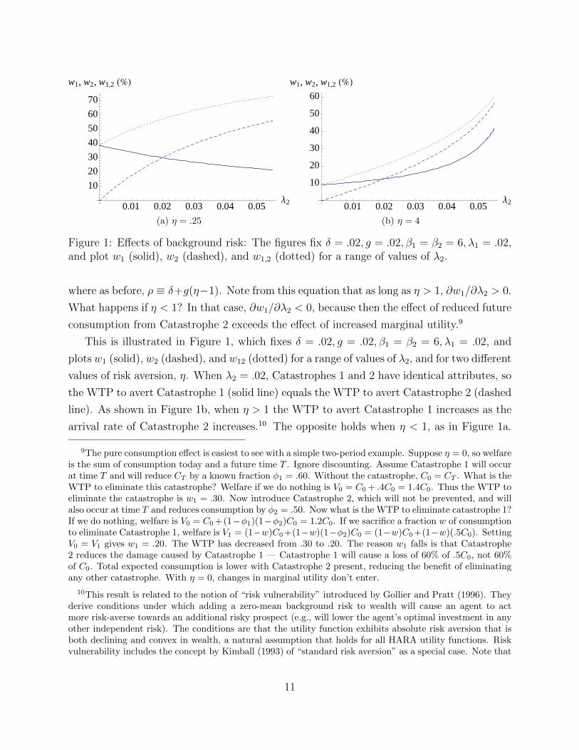
Figure 1: Effects of background risk: The figures fix δ = .02, g = .02, β1 = β2 = 6, λ1 = .02,and plot w1 (solid), w2 (dashed), and w1,2 (dotted) for a range of values of λ2.

where as before, ρ ≡ δ+g(η−1). Note from this equation that as long as η > 1, ∂w1/∂λ2 > 0.

What happens if η < 1? In that case, ∂w1/∂λ2 < 0, because then the effect of reduced future

consumption from Catastrophe 2 exceeds the effect of increased marginal utility.9

This is illustrated in Figure 1, which fixes δ = .02, g = .02, β1 = β2 = 6, λ1 = .02, and

plots w1 (solid), w2 (dashed), and w12 (dotted) for a range of values of λ2, and for two different

values of risk aversion, η. When λ2 = .02, Catastrophes 1 and 2 have identical attributes, so

the WTP to avert Catastrophe 1 (solid line) equals the WTP to avert Catastrophe 2 (dashed

line). As shown in Figure 1b, when η > 1 the WTP to avert Catastrophe 1 increases as the

arrival rate of Catastrophe 2 increases.10 The opposite holds when η < 1, as in Figure 1a.

9The pure consumption effect is easiest to see with a simple two-period example. Suppose η = 0, so welfareis the sum of consumption today and a future time T . Ignore discounting. Assume Catastrophe 1 will occurat time T and will reduce CT by a known fraction φ1 = .60. Without the catastrophe, C0 = CT . What is theWTP to eliminate this catastrophe? Welfare if we do nothing is V0 = C0 + .4C0 = 1.4C0. Thus the WTP toeliminate the catastrophe is w1 = .30. Now introduce Catastrophe 2, which will not be prevented, and willalso occur at time T and reduces consumption by φ2 = .50. Now what is the WTP to eliminate catastrophe 1?If we do nothing, welfare is V0 = C0 +(1−φ1)(1−φ2)C0 = 1.2C0. If we sacrifice a fraction w of consumptionto eliminate Catastrophe 1, welfare is V1 = (1−w)C0+(1−w)(1−φ2)C0 = (1−w)C0+(1−w)(.5C0). SettingV0 = V1 gives w1 = .20. The WTP has decreased from .30 to .20. The reason w1 falls is that Catastrophe2 reduces the damage caused by Catastrophe 1 — Catastrophe 1 will cause a loss of 60% of .5C0, not 60%of C0. Total expected consumption is lower with Catastrophe 2 present, reducing the benefit of eliminatingany other catastrophe. With η = 0, changes in marginal utility don’t enter.

10This result is related to the notion of “risk vulnerability” introduced by Gollier and Pratt (1996). Theyderive conditions under which adding a zero-mean background risk to wealth will cause an agent to actmore risk-averse towards an additional risky prospect (e.g., will lower the agent’s optimal investment in anyother independent risk). The conditions are that the utility function exhibits absolute risk aversion that isboth declining and convex in wealth, a natural assumption that holds for all HARA utility functions. Riskvulnerability includes the concept by Kimball (1993) of “standard risk aversion” as a special case. Note that

11

We will see below that when η = 1 (log utility), WTPs to avert different catastrophes are

independent of other background risks.

Unless noted otherwise, in the rest of this paper we will assume that η > 1. This is

consistent with both the finance and macroeconomics literatures, which put η in the range

of 2 to 5 (or even higher).

The next step is to link w1,2 to the individual WTPs w1 and w2. The key to doing so is

to note that since κ(1)(θ) + κ(2)(θ) = κ(θ) + κ(1,2)(θ), we have

1 + (1− w1,2)1−η = (1− w1)

1−η + (1− w2)1−η. (11)

Thus we can express the WTP to eliminate both types of catastrophes, w1,2 in terms of w1

and w2. But note that these WTPs do not add. In fact we can now show that w1,2 < w1+w2.

Clearly this must be the case if w1 + w2 > 1, so assume that w1 + w2 ≤ 1. Equation (11)

implies that w1,2 < w1 + w2 if 1 + (1 − w1 − w2)1−η > (1 − w1)

1−η + (1 − w2)1−η. But this

holds by convexity of the function x1−η, which gives the result.

2.2 Which Catastrophes to Avert?

Suppose we know the cost of averting each of these two catastrophes, expressed as a per-

manent consumption tax at rate τi. We can now ask which, if any, of the two catastrophes

should society avert? If τi > wi, then we should not avert catastrophe i. To make this

interesting, we will assume that τi < wi for both i = 1 and 2. Thus it is clearly optimal to

avert at least one of the catastrophes, but is it optimal to avert both?

To address this question, it will be useful to express the costs and benefits τi and wi in

terms of changes in utility rather than percentages of consumption. To do so, define

Ki = (1− τi)1−η − 1

Bi = (1− wi)1−η − 1 . (12)

After appropriately normalizing the utility function, Ki has a simple interpretation as the

percentage loss of utility that results when consumption is reduced by the fraction τi, and

likewise for Bi; correspondingly, Ki/(η − 1) is the absolute change in utility, measured in

utils, when C is reduced by τi, and likewise for Bi/(η− 1). Note that Ki and Bi are positive

and increasing in τi and wi, respectively; and that Ki > Bi if and only if τi > wi.

These utility-based measures of costs and benefits have some useful characteristics. We

saw, for example, that WTPs do not add: if η > 1, then w1,2 < w1 + w2. Corresponding

in our model background risk is not zero-mean; background events always reduce consumption.

12

to equation (12), define B1,2 = (1 − w1,2)1−η − 1. Then, from equation (11) we see that

B1,2 = B1 + B2, i.e., the Bis do add. What about costs? The consumption tax needed to

avert both catastrophes is τ1,2 = 1−(1−τ1)(1−τ2). The corresponding utility-based measure

is K1,2 = (1− τ1,2)1−η − 1 = (1− τ1)1−η(1− τ2)1−η − 1. Thus 1 + K1,2 = (1 + K1)(1 + K2),

i.e., the costs multiply. These properties of the Bis and Kis—that benefits add and costs

multiply—will prove useful later when we generalize to N different catastrophes.

Given these measures of costs and benefits, we now turn to the question of which catas-

trophes should be averted. Suppose B1 is sufficiently greater than K1 that we will definitely

avert Catastrophe 1. Should we also avert Catastrophe 2? Only if the benefit-cost ratio

B2/K2 exceeds the following hurdle rate:

B2

K2

> 1 +B1 . (13)

Thus the fact that society is going to avert Catastrophe 1 increases the hurdle rate for

Catastrophe 2. Furthermore, the greater is the benefit B1, the greater is the increase in the

hurdle rate for Catastrophe 2. Notice that this logic also applies if B1 = B2 and K1 = K2;

thus it might be the case that only one of two identical catastrophes should be averted.

If this result seems counter-intuitive, remember that what matters for this decision is

the additional benefit from averting Catastrophe 2 relative to the cost. In WTP terms, i.e.,

measured as a percentage of consumption, that additional benefit is (w1,2 − w1)/(1 − w1).

Substituting in the definitions of Ki and Bi, we can see that equation (13) is equivalent to

w1,2 − w1

1− w1

> τ2 .

It can easily be the case that w2 > τ2 but (w1,2−w1)/(1−w1) < τ2. The reason is that these

are not marginal projects, and as a result, w1,2 < w1 + w2. This is what raises the hurdle

rate in equation (13). To avert Catastrophe 1, society is willing to give up the fraction w1

of consumption, so that the remaining consumption is lower and marginal utility is higher.

Thus the dollar loss (as opposed to the percentage loss) from Catastrophe 2 is reduced, and

the utility loss from the second tax τ2 is increased.

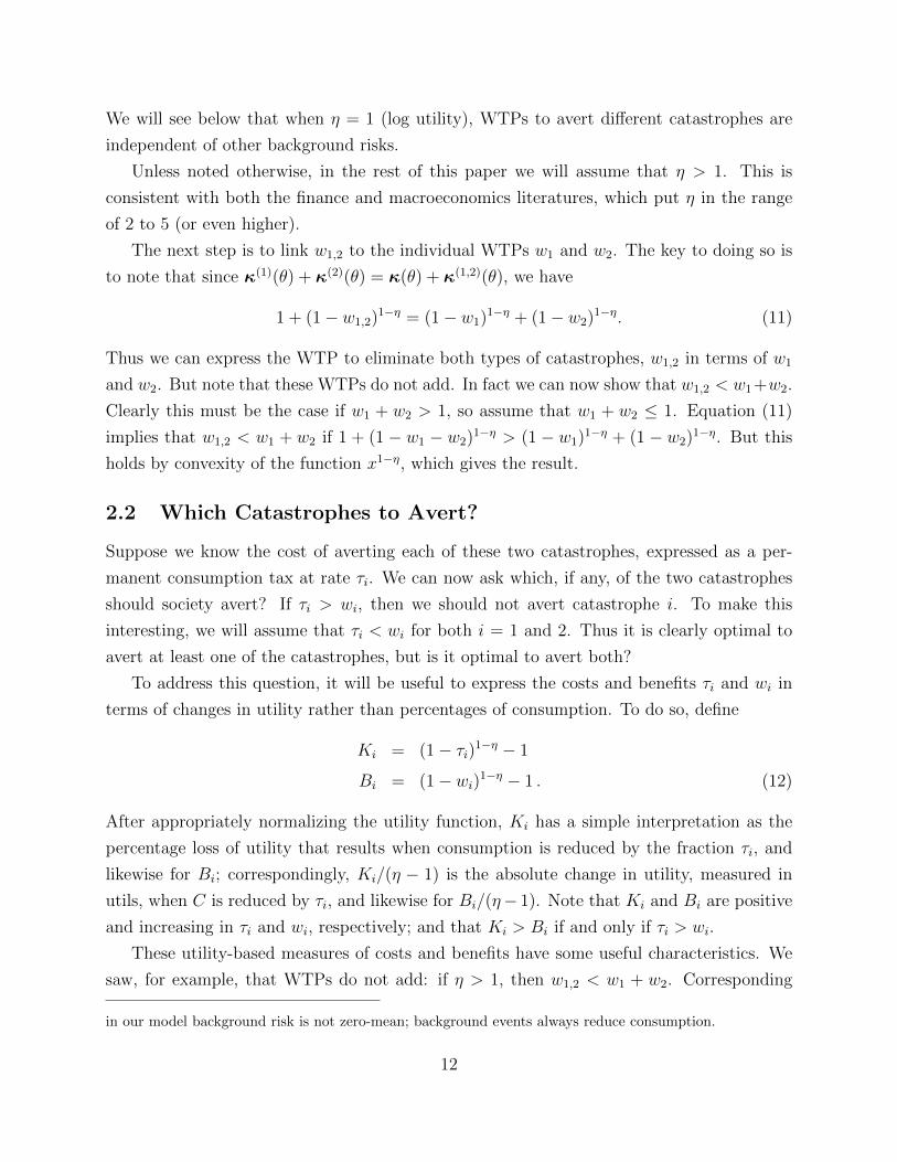
Example 1: Two Catastrophes. To illustrate this result, suppose τ1 = 20% and τ2 = 10%.

Figure 2 shows which catastrophes should be averted for a range of different values of w1

and w2. When wi < τi for both catastrophes (in the bottom left rectangle), neither should

be averted. We should avert both catastrophes only for combinations (w1, w2) in the middle

lozenge-shaped region. That region shrinks considerably when we increase η. In the context

of equation (13), the larger is η the larger is B1, and thus the larger is the hurdle rate for

averting the second catastrophe.

13

8<81<

81,2<

82<

0 20 40 60 80 1000

20

40

60

80

100

w1 H%L

w2

H%L

(a) η = 2

8<

81<

81,2<

82<

0 20 40 60 80 1000

20

40

60

80

100

w1 H%L

w2

H%L

(b) η = 3

Figure 2: There are two potential catastrophes, with τ1 = 20% and τ2 = 10%. The figuresshow, for all possible values of w1 and w2, which catastrophes should be averted (in curlybrackets). A catastrophe for which wi < τi should not be averted. We should avert bothcatastrophes only for combinations (w1, w2) in the middle shaded region. That region shrinksconsiderably when risk aversion, η, increases.

Consider, for example, the point (w1, w2) = (60%, 20%) in panel (b) of Figure 2. As

shown, we should avert only the first catastrophe even though w2 > τ2. In this case B1 =

5.25, B2 = 0.56, and K2 = 0.23, so B2/K2 = 2.39 < 1 + B1 = 6.25. Equivalently, w1,2 =

61.7%, so (w1,2−w1)/(1−w1) = 4.3% < τ2 = 10%. The additional benefit from also averting

Catastrophe 2 is less than the cost.

2.3 Marginal vs. “Non-Marginal” Projects

We have seen that the WTP to avert one catastrophe is affected by the presence of a second

catastrophe, even if that second catastrophe is not averted. Likewise, equation (13) shows

that averting one catastrophe increases the hurdle rate B/K that must be met to avert a

second catastrophe. As explained above, the reason is that the impact of each catastrophe

is “non-marginal,” as is the cost of a project to avert it. It is easy to see that these effects

disappear when the catastrophes (and the costs of averting them) are marginal, i.e., tiny in

relation to the overall economy.

For example, consider eqn. (10), which applies when zi = e−φi follows a power distribu-

tion, and the derivative ∂w1/∂λ2. The impact of a catastrophe is “tiny” when the parameter

β is very large. (A very large β implies a large E e−φ and thus a small expected impact.)

14

One can see from equation (10) that ∂w1/∂λ2 → 0 as β becomes very large.

Likewise, equation (13) says that the hurdle rate for averting Catastrophe 2 is B2/K2 =

1 + B1 = (1 − w1)1−η. But if the impact of Catastrophe 1 is tiny, so that w1 is very small,

(1− w1)1−η ≈ 1, and the usual cost-benefit criterion applies.

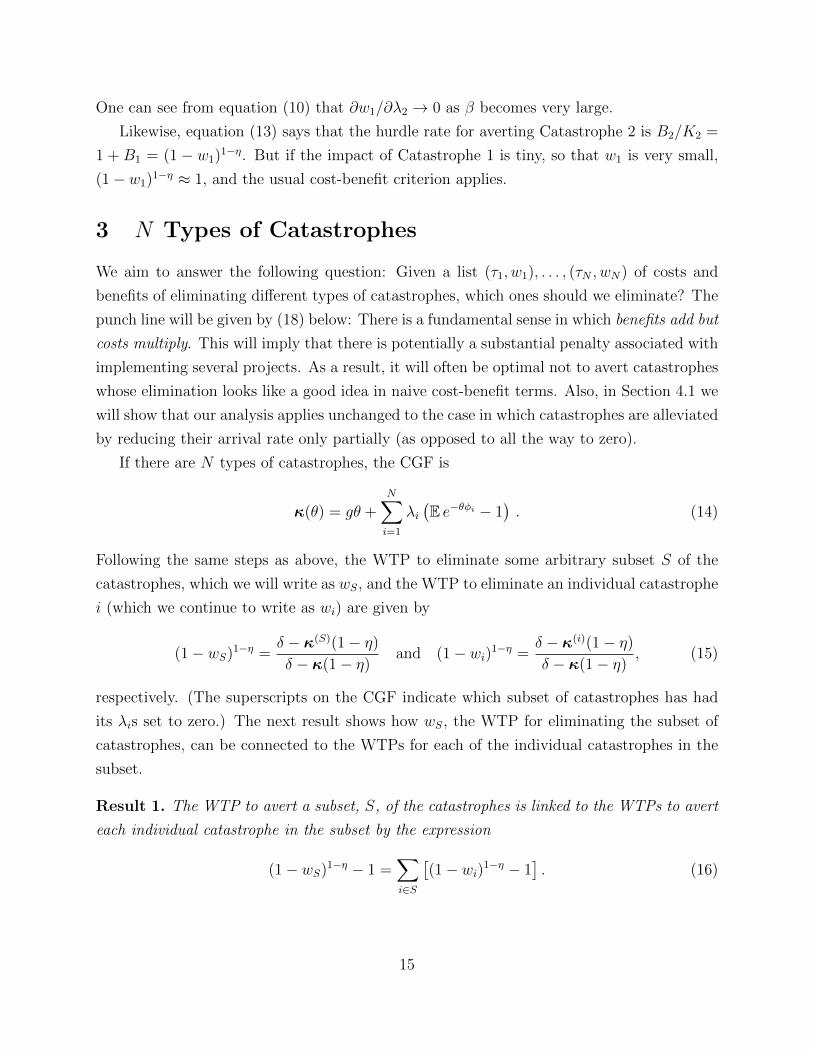
3 N Types of Catastrophes

We aim to answer the following question: Given a list (τ1, w1), . . . , (τN , wN) of costs and

benefits of eliminating different types of catastrophes, which ones should we eliminate? The

punch line will be given by (18) below: There is a fundamental sense in which benefits add but

costs multiply. This will imply that there is potentially a substantial penalty associated with

implementing several projects. As a result, it will often be optimal not to avert catastrophes

whose elimination looks like a good idea in naive cost-benefit terms. Also, in Section 4.1 we

will show that our analysis applies unchanged to the case in which catastrophes are alleviated

by reducing their arrival rate only partially (as opposed to all the way to zero).

If there are N types of catastrophes, the CGF is

κ(θ) = gθ +N∑i=1

λi(E e−θφi − 1

). (14)

Following the same steps as above, the WTP to eliminate some arbitrary subset S of the

catastrophes, which we will write as wS, and the WTP to eliminate an individual catastrophe

i (which we continue to write as wi) are given by

(1− wS)1−η =δ − κ(S)(1− η)

δ − κ(1− η)and (1− wi)1−η =

δ − κ(i)(1− η)

δ − κ(1− η), (15)

respectively. (The superscripts on the CGF indicate which subset of catastrophes has had

its λis set to zero.) The next result shows how wS, the WTP for eliminating the subset of

catastrophes, can be connected to the WTPs for each of the individual catastrophes in the

subset.

Result 1. The WTP to avert a subset, S, of the catastrophes is linked to the WTPs to avert

each individual catastrophe in the subset by the expression

(1− wS)1−η − 1 =∑i∈S

[(1− wi)1−η − 1

]. (16)

15

Proof. The result follows from a relationship between κ(S)(θ) and the individual κ(i)(θ). Note

that κ(i)(θ) = κ(θ) − λi(E e−θφi − 1

)and κ(S)(θ) = κ(θ) −

∑i∈S λi

(E e−θφi − 1

). (This is

effectively the definition of the notation κ(i) and κ(S).) Thus∑i∈S

κ(i)(θ) = |S|κ(θ)−∑i∈S

λi(E e−θφi − 1

)= (|S| − 1)κ(θ) + κ(S)(θ),

where |S| denotes the number of catastrophes in the subset S, and hence∑i∈S

δ − κ(i)(1− η)

δ − κ(1− η)=

(|S| − 1)(δ − κ(1− η)) + (δ − κ(S)(1− η))

δ − κ(1− η).

Using (15), we have the result.

For the case of N = 2, we showed that w1,2 ≤ w1 + w2 (with strict inequality if η > 1).

By the same reasoning, it can be shown that w1,2,...,N ≤∑N

i=1wi. Likewise, if we divide

the N catastrophes into two groups, 1 through M and M + 1 through N , then w1,2,...,N ≤w1,2,...,M + wM+1,...,N . The WTP to eliminate all N catastrophes will be less than the sum

of the WTPs for each of the individual catastrophes, and will be less than the sum of the

WTPs to eliminate any two groups of catastrophes.

3.1 Which Catastrophes to Avert?

The WTP, wi, measures the benefit of eliminating catastrophe i as the maximum fraction of

consumption society would sacrifice to achieve this result. We measure the cost of eliminating

the catastrophe as the actual fraction of consumption that would have to be sacrificed, via

a permanent consumption tax τi, to generate the revenue needed to avert the catastrophe.

Thus, if we eliminate some subset S of the catastrophes, welfare (net of taxes) is∏i∈S(1− τi)1−η

(1− η)(δ − κ(S)(1− η))=

∏i∈S(1− τi)1−η

(1− η)(δ − κ(1− η))(1− wS)1−η, (17)

where the equality follows from (15). Our goal is to pick the set of catastrophes to be

eliminated to maximize this expression.

The next result shows how to formulate an optimal policy given the costs τi and benefits

wi associated with different types of catastrophes. As for the case of N = 2, define

Ki = (1− τi)1−η − 1 and Bi = (1− wi)1−η − 1.

As before, Ki is the percentage loss of utility that results when consumption is reduced by

τi percent, and likewise for Bi; and dividing Ki (or Bi) by η − 1 gives the absolute loss (or

16

gain) in utils. These utility-based definitions of costs and benefits are positive and increasing

in τi and wi, respectively, and Ki > Bi if and only if τi > wi. For small τi, we have the

linearization Ki ≈ (η − 1)τi; and for small wi, we have Bi ≈ (η − 1)wi.

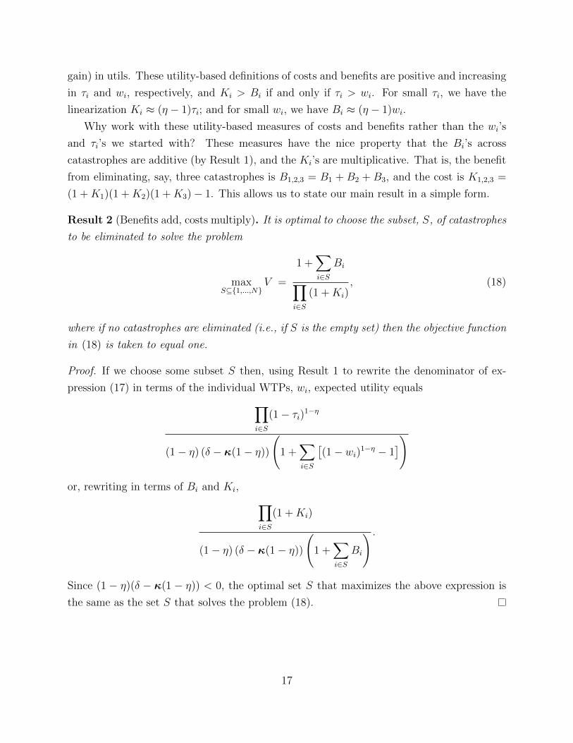
Why work with these utility-based measures of costs and benefits rather than the wi’s

and τi’s we started with? These measures have the nice property that the Bi’s across

catastrophes are additive (by Result 1), and the Ki’s are multiplicative. That is, the benefit

from eliminating, say, three catastrophes is B1,2,3 = B1 + B2 + B3, and the cost is K1,2,3 =

(1 +K1)(1 +K2)(1 +K3)− 1. This allows us to state our main result in a simple form.

Result 2 (Benefits add, costs multiply). It is optimal to choose the subset, S, of catastrophes

to be eliminated to solve the problem

maxS⊆{1,...,N}

V =

1 +∑i∈S

Bi∏i∈S

(1 +Ki), (18)

where if no catastrophes are eliminated (i.e., if S is the empty set) then the objective function

in (18) is taken to equal one.

Proof. If we choose some subset S then, using Result 1 to rewrite the denominator of ex-

pression (17) in terms of the individual WTPs, wi, expected utility equals∏i∈S

(1− τi)1−η

(1− η) (δ − κ(1− η))

(1 +

∑i∈S

[(1− wi)1−η − 1

])

or, rewriting in terms of Bi and Ki, ∏i∈S

(1 +Ki)

(1− η) (δ − κ(1− η))

(1 +

∑i∈S

Bi

) .

Since (1 − η)(δ − κ(1 − η)) < 0, the optimal set S that maximizes the above expression is

the same as the set S that solves the problem (18).

17

3.1.1 Many Small Catastrophes

It is problem (18) that generates the strange economics of the title. To understand how the

problem differs from what one might naively expect, notice that the set S solves

maxS

log

(1 +

∑i∈S

Bi

)−∑i∈S

log (1 +Ki).

One might think that if costs and benefits Ki and Bi are all small, then—since log(1+x) ≈ x

for small x—this problem could be closely approximated by the simpler problem

maxS

∑i∈S

(Bi −Ki). (19)

This linearized problem is separable, which vastly simplifies its solution: a catastrophe should

be eliminated if and only if the benefit of doing so, Bi, exceeds the cost, Ki. But the

linearized problem is only a tolerable approximation to the true problem if the total number

of catastrophes is limited, and in particular, if∑

i∈S Bi is small. It is not enough for the Bis

to be individually small. The reason is that averting a large number of small catastrophes

has the same aggregate impact on consumption (and marginal utility) as does averting a few

large catastrophes. We illustrate this with the following example.

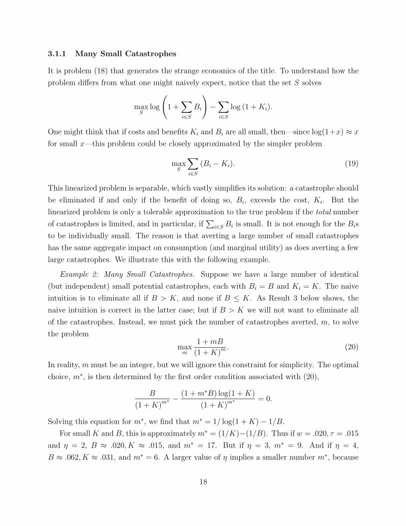
Example 2: Many Small Catastrophes. Suppose we have a large number of identical

(but independent) small potential catastrophes, each with Bi = B and Ki = K. The naive

intuition is to eliminate all if B > K, and none if B ≤ K. As Result 3 below shows, the

naive intuition is correct in the latter case; but if B > K we will not want to eliminate all

of the catastrophes. Instead, we must pick the number of catastrophes averted, m, to solve

the problem

maxm

1 +mB

(1 +K)m. (20)

In reality, m must be an integer, but we will ignore this constraint for simplicity. The optimal

choice, m∗, is then determined by the first order condition associated with (20),

B

(1 +K)m∗ −

(1 +m∗B) log(1 +K)

(1 +K)m∗ = 0.

Solving this equation for m∗, we find that m∗ = 1/ log(1 +K)− 1/B.

For small K and B, this is approximately m∗ = (1/K)−(1/B). Thus if w = .020, τ = .015

and η = 2, B ≈ .020, K ≈ .015, and m∗ = 17. But if η = 3, m∗ = 9. And if η = 4,

B ≈ .062, K ≈ .031, and m∗ = 6. A larger value of η implies a smaller number m∗, because

18

the percentage drop in aggregate consumption, 1 − (1 − τ)m, results in a larger increase in

marginal utility, and thus a greater loss of utility from averting one additional catastrophe.

Does it matter how large is the “large number” of catastrophes in this example (assuming

it is larger than the number we will avert)? No, because we fixed the value of w and τ

(and hence B and K) for each catastrophe. However, if we go back a step and consider

what determines w, it could indeed matter. The catastrophes we do not avert represent

“background risk,” and we have seen that all else equal, more background risk makes w

larger (assuming η > 1). Thus we would expect w (and hence B) to be larger if we face 200

small catastrophes than if we face only 50.

3.1.2 Catastrophes of Arbitrary Size

With catastrophes of arbitrary size, the solution of problem (18) is much more complicated.

How does one find the set S in practice? As a general matter, one can search over every

possible subset of the catastrophes to find the subset that maximizes the objective function in

(18). It is this (highly unusual) feature of the problem that led us to say, in the introduction,

that there is an essential interdependence between catastrophes. With N catastrophes under

consideration there are 2N possible subsets to evaluate—a problem that rapidly becomes

computationally hard. There is a stark contrast with conventional cost-benefit analysis, in

which an individual project can be evaluated in isolation. Our general problem (18) reduces

to this case only if all disasters are very small, both individually and in aggregate, as in (19).

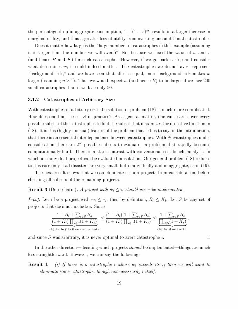
The next result shows that we can eliminate certain projects from consideration, before

checking all subsets of the remaining projects.

Result 3 (Do no harm). A project with wi ≤ τi should never be implemented.

Proof. Let i be a project with wi ≤ τi; then by definition, Bi ≤ Ki. Let S be any set of

projects that does not include i. Since

1 +Bi +∑

s∈S Bs

(1 +Ki)∏

s∈S(1 +Ks)︸ ︷︷ ︸obj. fn. in (18) if we avert S and i

≤(1 +Bi)(1 +

∑s∈S Bs)

(1 +Ki)∏

s∈S(1 +Ks)≤

1 +∑

s∈S Bs∏s∈S(1 +Ks)︸ ︷︷ ︸

obj. fn. if we avert S

,

and since S was arbitrary, it is never optimal to avert catastrophe i.

In the other direction—deciding which projects should be implemented—things are much

less straightforward. However, we can say the following:

Result 4. (i) If there is a catastrophe i whose wi exceeds its τi then we will want to

eliminate some catastrophe, though not necessarily i itself.

19

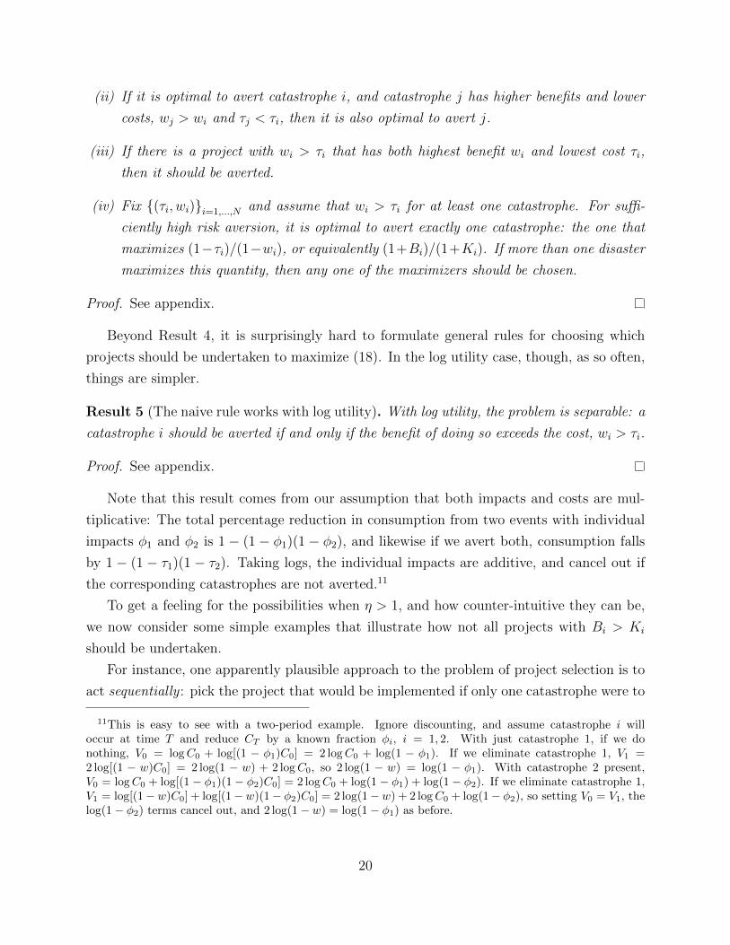
(ii) If it is optimal to avert catastrophe i, and catastrophe j has higher benefits and lower

costs, wj > wi and τj < τi, then it is also optimal to avert j.

(iii) If there is a project with wi > τi that has both highest benefit wi and lowest cost τi,

then it should be averted.

(iv) Fix {(τi, wi)}i=1,...,N and assume that wi > τi for at least one catastrophe. For suffi-

ciently high risk aversion, it is optimal to avert exactly one catastrophe: the one that

maximizes (1−τi)/(1−wi), or equivalently (1+Bi)/(1+Ki). If more than one disaster

maximizes this quantity, then any one of the maximizers should be chosen.

Proof. See appendix.

Beyond Result 4, it is surprisingly hard to formulate general rules for choosing which

projects should be undertaken to maximize (18). In the log utility case, though, as so often,

things are simpler.

Result 5 (The naive rule works with log utility). With log utility, the problem is separable: a

catastrophe i should be averted if and only if the benefit of doing so exceeds the cost, wi > τi.

Proof. See appendix.

Note that this result comes from our assumption that both impacts and costs are mul-

tiplicative: The total percentage reduction in consumption from two events with individual

impacts φ1 and φ2 is 1 − (1 − φ1)(1 − φ2), and likewise if we avert both, consumption falls

by 1 − (1 − τ1)(1 − τ2). Taking logs, the individual impacts are additive, and cancel out if

the corresponding catastrophes are not averted.11

To get a feeling for the possibilities when η > 1, and how counter-intuitive they can be,

we now consider some simple examples that illustrate how not all projects with Bi > Ki

should be undertaken.

For instance, one apparently plausible approach to the problem of project selection is to

act sequentially : pick the project that would be implemented if only one catastrophe were to

11This is easy to see with a two-period example. Ignore discounting, and assume catastrophe i willoccur at time T and reduce CT by a known fraction φi, i = 1, 2. With just catastrophe 1, if we donothing, V0 = logC0 + log[(1 − φ1)C0] = 2 logC0 + log(1 − φ1). If we eliminate catastrophe 1, V1 =2 log[(1 − w)C0] = 2 log(1 − w) + 2 logC0, so 2 log(1 − w) = log(1 − φ1). With catastrophe 2 present,V0 = logC0 + log[(1− φ1)(1− φ2)C0] = 2 logC0 + log(1− φ1) + log(1− φ2). If we eliminate catastrophe 1,V1 = log[(1−w)C0] + log[(1−w)(1− φ2)C0] = 2 log(1−w) + 2 logC0 + log(1− φ2), so setting V0 = V1, thelog(1− φ2) terms cancel out, and 2 log(1− w) = log(1− φ1) as before.

20

be eliminated and then—after implementing that project—continue, selecting the next most

desirable project; and so on. The next example shows that this approach is not optimal.

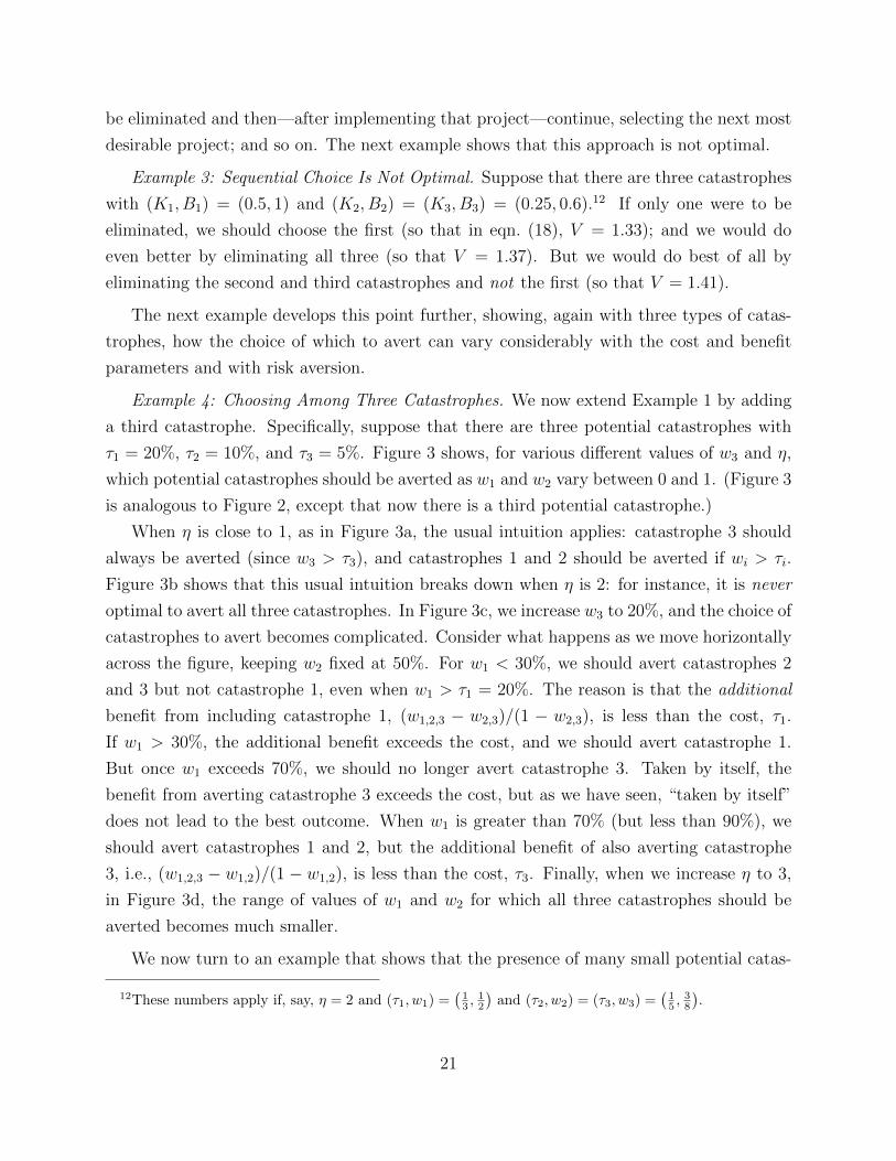
Example 3: Sequential Choice Is Not Optimal. Suppose that there are three catastrophes

with (K1, B1) = (0.5, 1) and (K2, B2) = (K3, B3) = (0.25, 0.6).12 If only one were to be

eliminated, we should choose the first (so that in eqn. (18), V = 1.33); and we would do

even better by eliminating all three (so that V = 1.37). But we would do best of all by

eliminating the second and third catastrophes and not the first (so that V = 1.41).

The next example develops this point further, showing, again with three types of catas-

trophes, how the choice of which to avert can vary considerably with the cost and benefit

parameters and with risk aversion.

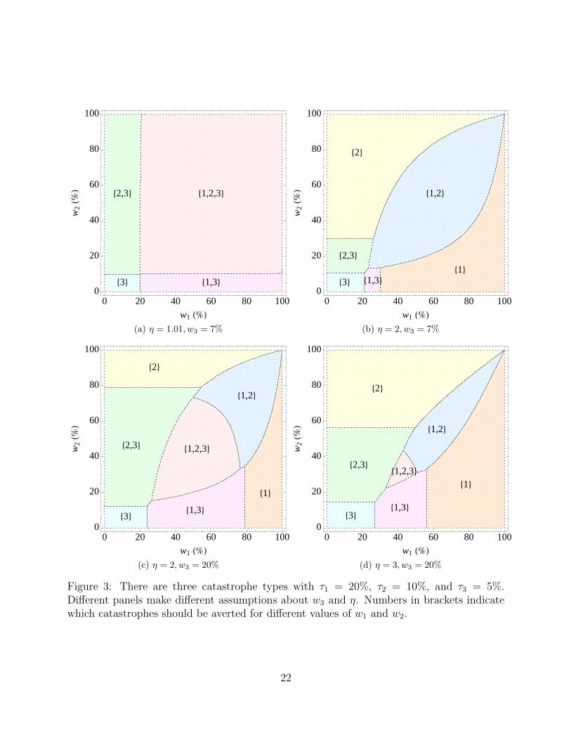
Example 4: Choosing Among Three Catastrophes. We now extend Example 1 by adding

a third catastrophe. Specifically, suppose that there are three potential catastrophes with

τ1 = 20%, τ2 = 10%, and τ3 = 5%. Figure 3 shows, for various different values of w3 and η,

which potential catastrophes should be averted as w1 and w2 vary between 0 and 1. (Figure 3

is analogous to Figure 2, except that now there is a third potential catastrophe.)

When η is close to 1, as in Figure 3a, the usual intuition applies: catastrophe 3 should

always be averted (since w3 > τ3), and catastrophes 1 and 2 should be averted if wi > τi.

Figure 3b shows that this usual intuition breaks down when η is 2: for instance, it is never

optimal to avert all three catastrophes. In Figure 3c, we increase w3 to 20%, and the choice of

catastrophes to avert becomes complicated. Consider what happens as we move horizontally

across the figure, keeping w2 fixed at 50%. For w1 < 30%, we should avert catastrophes 2

and 3 but not catastrophe 1, even when w1 > τ1 = 20%. The reason is that the additional

benefit from including catastrophe 1, (w1,2,3 − w2,3)/(1 − w2,3), is less than the cost, τ1.

If w1 > 30%, the additional benefit exceeds the cost, and we should avert catastrophe 1.

But once w1 exceeds 70%, we should no longer avert catastrophe 3. Taken by itself, the

benefit from averting catastrophe 3 exceeds the cost, but as we have seen, “taken by itself”

does not lead to the best outcome. When w1 is greater than 70% (but less than 90%), we

should avert catastrophes 1 and 2, but the additional benefit of also averting catastrophe

3, i.e., (w1,2,3 − w1,2)/(1 − w1,2), is less than the cost, τ3. Finally, when we increase η to 3,

in Figure 3d, the range of values of w1 and w2 for which all three catastrophes should be

averted becomes much smaller.

We now turn to an example that shows that the presence of many small potential catas-

12These numbers apply if, say, η = 2 and (τ1, w1) =(13 ,

12

)and (τ2, w2) = (τ3, w3) =

(15 ,

38

).

21

83<

82,3< 81,2,3<

81,3<

0 20 40 60 80 1000

20

40

60

80

100

w1 H%L

w2

H%L

(a) η = 1.01, w3 = 7%

83<81<

82,3<

81,2<

81,3<

82<

0 20 40 60 80 1000

20

40

60

80

100

w1 H%L

w2

H%L

(b) η = 2, w3 = 7%

83<

81<

82,3< 81,2,3<

81,2<

81,3<

82<

0 20 40 60 80 1000

20

40

60

80

100

w1 H%L

w2

H%L

(c) η = 2, w3 = 20%

83<

81<

82,3<81,2,3<

81,2<

81,3<

82<

0 20 40 60 80 1000

20

40

60

80

100

w1 H%L

w2

H%L

(d) η = 3, w3 = 20%

Figure 3: There are three catastrophe types with τ1 = 20%, τ2 = 10%, and τ3 = 5%.Different panels make different assumptions about w3 and η. Numbers in brackets indicatewhich catastrophes should be averted for different values of w1 and w2.

22

trophes raises the hurdle rate required to act to prevent a large potential catastrophe. In

particular, it may be best not to eliminate the large catastrophe, even if the benefit of

elimination exceeds the cost.

Example 5: Multiple Small Catastrophes Can Crowd Out a Large Catastrophe. Suppose

that there are many small, independent, catastrophes, each with cost k and benefit b, and

one large catastrophe with cost K and benefit B. Then we must compare

maxm

1 +mb

(1 + k)mwith max

m

1 +B +mb

(1 +K)(1 + k)m.

Ignoring the integer constraint, and assuming that it is optimal to eliminate at least one

small catastrophe, the optimized values of these problems are

b(1 + k)1/b

e log(1 + k)and

b(1 + k)(1+B)/b

e(1 +K) log(1 + k),

respectively. It follows that we should eliminate the large catastrophe if and only if

B

log(1 +K)>

b

log(1 + k). (21)

If the costs of eliminating all catastrophes are small enough that we can use the approx-

imation log(1 + x) ≈ x, then the criterion is essentially that we should avert the large

catastrophe if and only if B/K > b/k. For small B, K, b, and k, this is equivalent to

W/T > w/τ (where for example W denotes WTP to eliminate the large catastrophe and τ

the cost of eliminating the small catastrophe). Thus the hurdle rate for elimination of the

large catastrophe is increased by virtue of the presence of the small catastrophes.

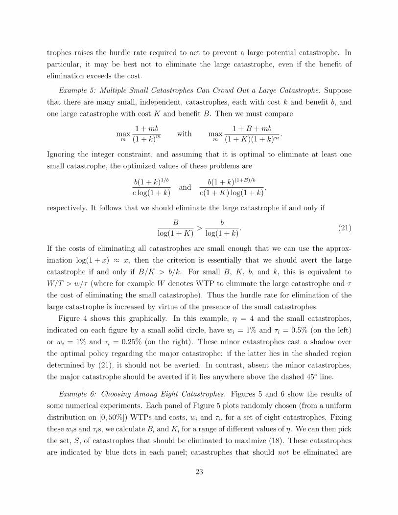
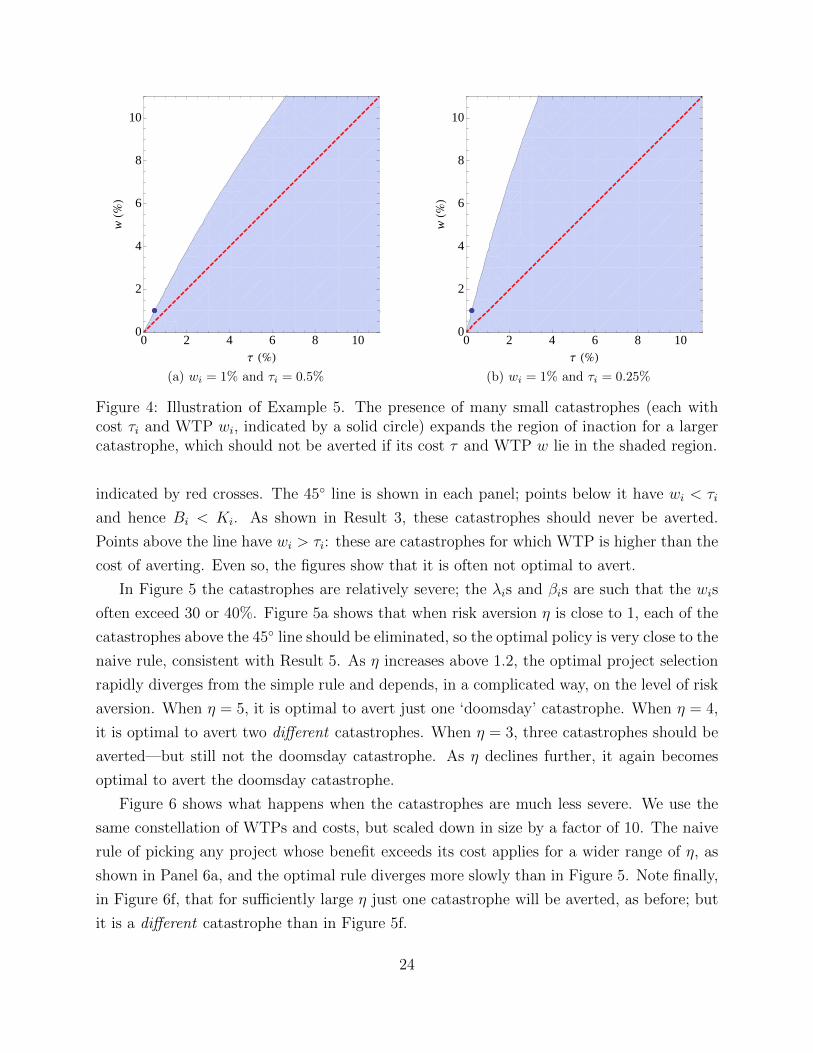
Figure 4 shows this graphically. In this example, η = 4 and the small catastrophes,

indicated on each figure by a small solid circle, have wi = 1% and τi = 0.5% (on the left)

or wi = 1% and τi = 0.25% (on the right). These minor catastrophes cast a shadow over

the optimal policy regarding the major catastrophe: if the latter lies in the shaded region

determined by (21), it should not be averted. In contrast, absent the minor catastrophes,

the major catastrophe should be averted if it lies anywhere above the dashed 45◦ line.

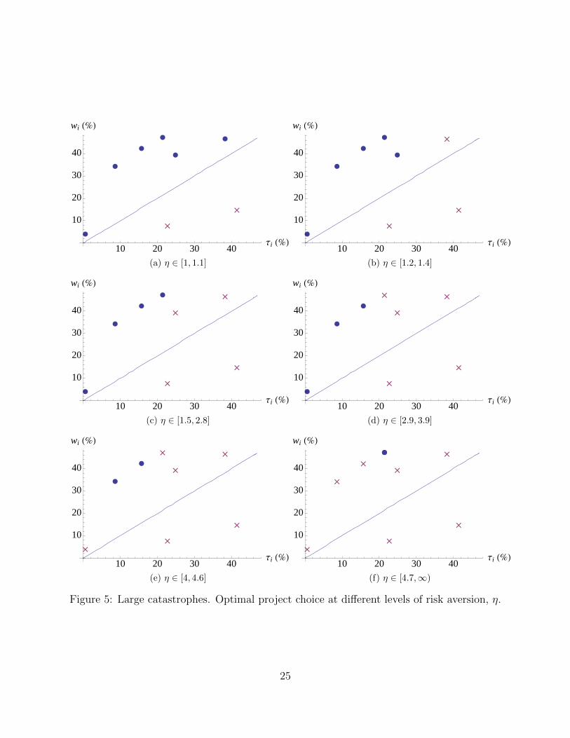
Example 6: Choosing Among Eight Catastrophes. Figures 5 and 6 show the results of

some numerical experiments. Each panel of Figure 5 plots randomly chosen (from a uniform

distribution on [0, 50%]) WTPs and costs, wi and τi, for a set of eight catastrophes. Fixing

these wis and τis, we calculate Bi and Ki for a range of different values of η. We can then pick

the set, S, of catastrophes that should be eliminated to maximize (18). These catastrophes

are indicated by blue dots in each panel; catastrophes that should not be eliminated are

23

èè

0 2 4 6 8 100

2

4

6

8

10

Τ H%L

wH%

L

(a) wi = 1% and τi = 0.5%

èè

0 2 4 6 8 100

2

4

6

8

10

Τ H%L

wH%

L

(b) wi = 1% and τi = 0.25%

Figure 4: Illustration of Example 5. The presence of many small catastrophes (each withcost τi and WTP wi, indicated by a solid circle) expands the region of inaction for a largercatastrophe, which should not be averted if its cost τ and WTP w lie in the shaded region.

indicated by red crosses. The 45◦ line is shown in each panel; points below it have wi < τi

and hence Bi < Ki. As shown in Result 3, these catastrophes should never be averted.

Points above the line have wi > τi: these are catastrophes for which WTP is higher than the

cost of averting. Even so, the figures show that it is often not optimal to avert.

In Figure 5 the catastrophes are relatively severe; the λis and βis are such that the wis

often exceed 30 or 40%. Figure 5a shows that when risk aversion η is close to 1, each of the

catastrophes above the 45◦ line should be eliminated, so the optimal policy is very close to the

naive rule, consistent with Result 5. As η increases above 1.2, the optimal project selection

rapidly diverges from the simple rule and depends, in a complicated way, on the level of risk

aversion. When η = 5, it is optimal to avert just one ‘doomsday’ catastrophe. When η = 4,

it is optimal to avert two different catastrophes. When η = 3, three catastrophes should be

averted—but still not the doomsday catastrophe. As η declines further, it again becomes

optimal to avert the doomsday catastrophe.

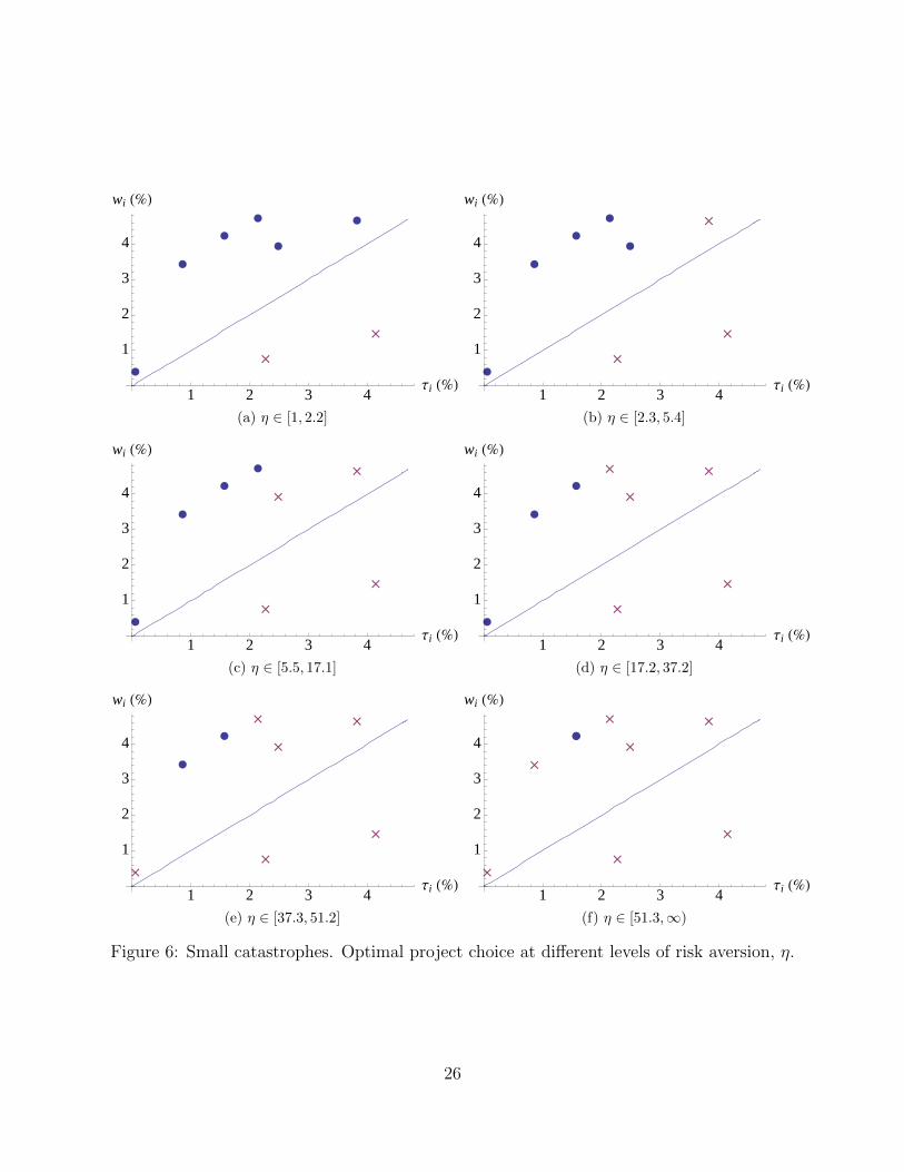
Figure 6 shows what happens when the catastrophes are much less severe. We use the

same constellation of WTPs and costs, but scaled down in size by a factor of 10. The naive

rule of picking any project whose benefit exceeds its cost applies for a wider range of η, as

shown in Panel 6a, and the optimal rule diverges more slowly than in Figure 5. Note finally,

in Figure 6f, that for sufficiently large η just one catastrophe will be averted, as before; but

it is a different catastrophe than in Figure 5f.

24

è è

è

è

è

è

�

�

10 20 30 40Τi H%L

10

20

30

40

wi H%L

(a) η ∈ [1, 1.1]

è

è

è

è

è

�

�

�

10 20 30 40Τi H%L

10

20

30

40

wi H%L

(b) η ∈ [1.2, 1.4]

è

è

è

è

�

�

�

�

10 20 30 40Τi H%L

10

20

30

40

wi H%L

(c) η ∈ [1.5, 2.8]

è

è

è

�

� �

�

�

10 20 30 40Τi H%L

10

20

30

40

wi H%L

(d) η ∈ [2.9, 3.9]

è

è

�

� �

�

�

�

10 20 30 40Τi H%L

10

20

30

40

wi H%L

(e) η ∈ [4, 4.6]

èè

�

�

��

�

�

�

10 20 30 40Τi H%L

10

20

30

40

wi H%L

(f) η ∈ [4.7,∞)

Figure 5: Large catastrophes. Optimal project choice at different levels of risk aversion, η.

25

è è

è

è

è

è

�

�

1 2 3 4Τi H%L

1

2

3

4

wi H%L

(a) η ∈ [1, 2.2]

è

è

è

è

è

�

�

�

1 2 3 4Τi H%L

1

2

3

4

wi H%L

(b) η ∈ [2.3, 5.4]

è

è

è

è

�

�

�

�

1 2 3 4Τi H%L

1

2

3

4

wi H%L

(c) η ∈ [5.5, 17.1]

è

è

è

�

� �

�

�

1 2 3 4Τi H%L

1

2

3

4

wi H%L

(d) η ∈ [17.2, 37.2]

è

è

�

� �

�

�

�

1 2 3 4Τi H%L

1

2

3

4

wi H%L

(e) η ∈ [37.3, 51.2]

èè

�

� �

�

�

�

�

1 2 3 4Τi H%L

1

2

3

4

wi H%L

(f) η ∈ [51.3,∞)

Figure 6: Small catastrophes. Optimal project choice at different levels of risk aversion, η.

26

4 Extensions

Thus far, we have made various assumptions to keep things simple. We have taken an ‘all-

or-nothing’ approach to alleviating catastrophes: a catastrophe is averted entirely or not at

all. We have assumed that a policy to avert catastrophe A has no effect on the likelihood of

catastrophe B. And we have assumed that catastrophes are, well, catastrophes, that is, bad

news. This section shows that all three assumptions are inessential. We can allow for partial,

as opposed to total, alleviation of catastrophes; we can allow for the possibility that a policy

to avert (say) nuclear terrorism decreases the likelihood of bio-terrorism; and we can use

the framework to consider optimal policies with respect to potential bonanzas—policies such

as blue-sky research or infrastructure investment that increase the probability of something

good happening (as opposed to decreasing the probability of something bad happening).

4.1 Partial Alleviation of Catastrophes

As a practical matter, the complete elimination of some catastrophes may be impossible or

prohibitively expensive. A more feasible alternative may be to reduce the likelihood that the

catastrophe will occur, i.e., to reduce the Poisson arrival rate λ. For example, Allison (2004)

suggests that the annual probability of a nuclear terrorist attack is λ ≈ .07. While reducing

the probability to zero may not be possible, we might be able to reduce λ substantially at a

cost that is less than the benefit. Should we do that, and how would the answer change if

we are also considering reducing the arrival rates for other potential catastrophes?

Our analysis of multiple catastrophes makes this problem easy to deal with. We consider

the possibility of reducing the arrival rate of some catastrophe from λ to λ(1− p), which we

call “alleviating the catastrophe by probability p.” We write w1(p) for the WTP to do just

that for the first type of catastrophe. Thus w1, in our earlier notation, is equal to w1(1).

We consider two forms of partial alleviation. First, suppose there are specific policies that

alleviate a given catastrophe type by some probability; an example is the rigorous inspection

of shipping containers. This implies a discrete set of policies to consider, and the previous

analysis goes through essentially unmodified. Second, we allow the probability by which the

catastrophe is alleviated to be chosen optimally. Perhaps surprisingly, the discrete flavor of

our earlier results still hold, and those results are almost unchanged.

4.1.1 Discrete partial alleviation

To find the WTP to alleviate the first type of catastrophe by probability p, that is, w1(p), we

make use of a property of Poisson processes. We can split the ‘type-1’ catastrophe into two

27

subsidiary types: 1a (arriving at rate λ1a ≡ λ1p) and 1b (arriving at rate λ1b ≡ λ1(1− p)).13

Thus we can rewrite the CGF (14) in the equivalent form:

κ(θ) = gθ + λ1a(E e−θφ1 − 1

)︸ ︷︷ ︸type 1a, arriving at rate λ1a

+ λ1b(E e−θφ1 − 1

)︸ ︷︷ ︸type 1b, arriving at rate λ1b

+N∑i=2

λi(E e−θφi − 1

)︸ ︷︷ ︸

all other types

,

so that alleviating catastrophe 1 by probability p corresponds to setting λ1a to zero, and

alleviating catastrophe 1 by probability 1 − p corresponds to setting λ1b to zero. This fits

the partial alleviation problem into our framework. For example, Result 1 implies that

1 + (1− w1(1))1−η = (1− w1(p))1−η + (1− w1(1− p))1−η

and the argument below equation (11) implies that w1(p)+w1(1−p) > w1(1) for all p ∈ (0, 1).

For example, w1

(12

)> 1

2w1(1): the WTP to reduce the likelihood of the catastrophe by half

is more than half the WTP to eliminate it entirely.

More generally, we can split up each type of catastrophe into two or more subtypes.

Suppose, for example, that catastrophe #2 can be alleviated by 20% at some cost, and by

30% at some other cost, but it cannot be averted fully. We can then split this into three

subtypes: type 2a catastrophes, arriving at rate 0.2 × λ2, which can be averted at cost

τ2a < 1; type 2b catastrophes, arriving at rate 0.3×λ2, which can be averted at cost τ2b < 1;

and type 2c catastrophes, arriving at rate 0.5×λ2, which can be averted at cost τ2c = 1, i.e.,

at infinite utility cost.

The next result links the WTP to alleviate a catastrophe by some probability to the

WTP to avert fully.

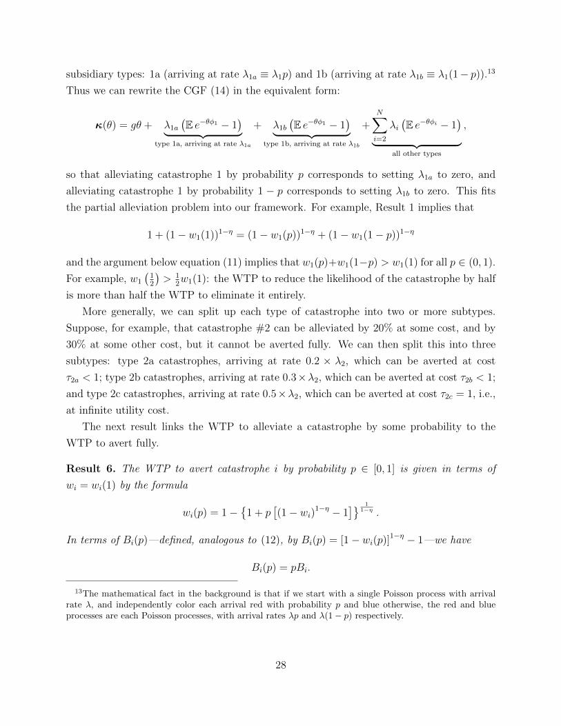
Result 6. The WTP to avert catastrophe i by probability p ∈ [0, 1] is given in terms of

wi = wi(1) by the formula

wi(p) = 1−{

1 + p[(1− wi)1−η − 1

]} 11−η .

In terms of Bi(p)—defined, analogous to (12), by Bi(p) = [1− wi(p)]1−η − 1—we have

Bi(p) = pBi.

13The mathematical fact in the background is that if we start with a single Poisson process with arrivalrate λ, and independently color each arrival red with probability p and blue otherwise, the red and blueprocesses are each Poisson processes, with arrival rates λp and λ(1− p) respectively.

28

Proof. As shown above, we can split the original catastrophe (arriving at rate λ) into N

different catastrophes, each arriving at rate λ/N , and link the cost of eliminating each of

these individually to the cost of eliminating the overall catastrophe. From equation (16),

N[(1− wi(1/N))1−η − 1

]= (1− wi)1−η − 1, and hence

wi(1/N) = 1−{

1 +1

N

[(1− wi)1−η − 1

]} 11−η

. (22)

This establishes the result when p = 1/N , for integer N . Next we extend to rationals, M/N .

But this follows immediately because, using equation (16) again, M[(1− wi(1/N))1−η − 1

]=

(1− wi(M/N))1−η − 1, and so, using (22),

wi(M/N) = 1−{

1 +M

N

[(1− wi)1−η − 1

]} 11−η

.

This establishes the result for arbitrary rational p. Finally, since WTP is a continuous

function of p, and since the rationals are dense in the reals, the result holds for all p; and it

is immediate that the formula for wi(p) is equivalent to the formula for Bi(p).

To summarize, once catastrophe types are defined appropriately, our framework accom-

modates without modification policies to alleviate catastrophes by some probability.

4.1.2 Optimal partial alleviation

Now we allow the probability by which a given catastrophe is alleviated to be chosen freely.

We assume that for each catastrophe i, we are given the WTP wi—which implicitly defines

wi(p), by Result 6—and the cost function, τi(p), associated with alleviating by probability p.

For now we do not specify the particular form of τi(p), but below we will consider a natural

special case in which τi(p) is determined as a function of τi ≡ τi(1) and p in much the same

way as wi(p) is determined by wi ≡ wi(1) and p.

Defining Ki(p) = (1− τi(p))1−η − 1, the optimization problem is to

maxpj∈[0,1]

1 +∑N

j=1Bj(pj)∏Nj=1 (1 +Kj(pj))

.

This is equivalent, by Result 6, to

maxpj∈[0,1]

log

(1 +

N∑j=1

pjBj

)−

N∑j=1

log (1 +Kj(pj)) .

29

Defining ki(p) = log(1 +Ki(p)), the problem becomes

maxpj∈[0,1]

log

(1 +

N∑j=1

pjBj

)−

N∑j=1

kj(pj).

If the functions kj(·) are convex, which we now assume is the case, then this is a con-

vex problem, so that the Kuhn–Tucker conditions are necessary and sufficient. Attaching

multipliers γj to the constraints pj − 1 ≤ 0 and µj to the constraints −pj ≤ 0, we have the

following necessary and sufficient conditions: for all j, we have γj ≥ 0 and µj ≥ 0, and

Bj

1 +∑

i piBi

− k′j(pj) = γj − µj where γj(pj − 1) = 0 and µjpj = 0.

The latter two (complementary slackness) conditions imply that pj = 1 if γj > 0 and pj = 0

if µj > 0. For any fixed j, at most one of γj and µj can be positive.

To analyze the problem further, we now consider two alternative assumptions about the

shapes of the cost functions ki(p).

Alternative 1: Inada-type conditions on ki(p). Suppose that k′j(0) = 0 and k′j(1) = ∞.

Then we can rule out corner solutions, so all Lagrange multipliers are zero and

Bj

k′j(pj)= 1 +

∑i

piBi for each j. (23)

From the definition of ki(·), k′j(pj) = K ′j(pj)/[1+Kj(pj)], so—assuming it is optimal to avert

at least one catastrophe, so that 1 +∑

i piBi >∏N

j=1(1 + Kj(pj)) and hence 1 +∑

i piBi >

1 + Kj(pj) for all j—condition (23) implies that Bj > K ′j(pj) at any interior optimum.14

Compare this with the corresponding condition in the naive problem maxpj∑

j Bj(pj) −∑jKj(pj), which is that Bj = K ′j(pj). Once again, the presence of multiple catastrophes

raises the hurdle rate, but now for an increase in pj, i.e., greater alleviation.

Alternative 2: A benchmark functional form for ki(p). Suppose that

(1− τi(p))(1− τi(q)) = 1− τi(p+ q) for all p, q, and i,

so that ‘alleviating by p’ and then ‘alleviating by q’ is as costly as ‘alleviating by p + q’ in

one go. This is a technological assumption. It might hold if a deadly virus comes from goats

or chimps, and funds can be devoted to goat research, chimp research, or both. In other

cases, it might not hold: there might be a finite cost of alleviating by 0.5 but an infinite cost

of fully averting.

14Remember that Bj = Bj(1) is a number, not a function; since Bj(pj) = pjBj , from Result 6, we canalso interpret Bj as the marginal benefit of an increase in pj , that is, B′j(pj).

30

This assumption pins down the form of the cost function: writing τi(1) = τi, we must

have τi(p) = 1 − (1 − τi)p or, equivalently, 1 + Ki(p) = (1 + Ki)

p. This implies that the

functions ki(·) defined above are linear:

ki(pi) = log(1 +Ki(pi)) = piki, (24)

where ki ≡ log(1 +Ki). Thus k′j(pj) = kj, an exogenous constant independent of pj.

By analyzing the Kuhn–Tucker conditions, the set of catastrophes can be divided into

three groups. First, there are catastrophes j that should not be averted even partially (so

that pj = 0). For these catastrophes the cost-benefit tradeoff is unattractive, in that

Bj

kj< 1 +

∑i

piBi.

Then there are the catastrophes that should be fully averted. These are catastrophes j that

pass a certain hurdle rate,Bj

kj> 1 +

∑i

piBi.

Finally, there may be interior solutions, catastrophes that are partially averted, pj ∈ [0, 1].

These must satisfyBj

kj= 1 +

∑i

piBi.

Catastrophes are therefore categorized by the benefit-cost ratios Bj/kj. These can be

thought of as parameters of the policy choice problem. If, by coincidence, two or more

different types of catastrophes have the same ratio Bj/kj, then we may have two or more

types of catastrophe that are partially alleviated. But generically, all catastrophes will have

different values of Bj/kj and so at most one catastrophe should be partially alleviated ; the

remainder are all-or-nothing, and should be fully averted if their benefit-cost ratio exceeds

the critical hurdle rate X ≡ 1 +∑

i piBi, and not averted at all if their benefit-cost ratio is

less than X. The interdependence manifests itself through the fact that the hurdle rate X is

dependent on the characteristics of, and optimal policies regarding, all the catastrophes.15

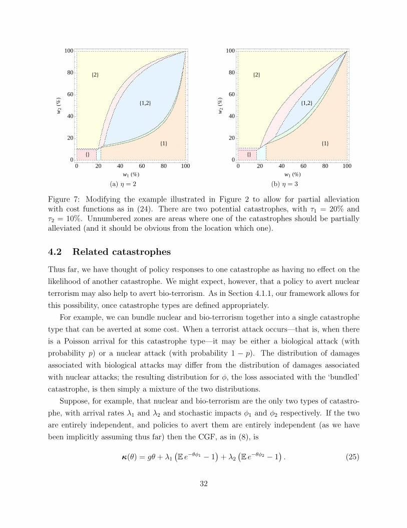
This is illustrated in Figure 7, which makes the same assumptions about wi and τi as in

Figure 2; the only difference is that we now allow for optimal partial alleviation, with cost

functions ki(p) as in (24). The basic intuition is not altered by partial alleviation.

15This characterization fails in the all-or-nothing case, as can be seen by considering an example with twocatastrophes and B1 = 8, K1 = 0.4, B2 = 36, K2 = 4. The optimal policy with partial alleviation is to avertcatastrophe 1 fully, and catastrophe 2 with probability 0.371. Correspondingly, catastrophe 2 has a lowerBj/kj . But in the all-or-nothing case, it is best to avert catastrophe 2 and not catastrophe 1.

31

8<

81<

82<

81,2<

0 20 40 60 80 1000

20

40

60

80

100

w1 H%L

w2

H%L

(a) η = 2

8<

81<

82<

81,2<

0 20 40 60 80 1000

20

40

60

80

100

w1 H%L

w2

H%L

(b) η = 3

Figure 7: Modifying the example illustrated in Figure 2 to allow for partial alleviationwith cost functions as in (24). There are two potential catastrophes, with τ1 = 20% andτ2 = 10%. Unnumbered zones are areas where one of the catastrophes should be partiallyalleviated (and it should be obvious from the location which one).

4.2 Related catastrophes

Thus far, we have thought of policy responses to one catastrophe as having no effect on the

likelihood of another catastrophe. We might expect, however, that a policy to avert nuclear

terrorism may also help to avert bio-terrorism. As in Section 4.1.1, our framework allows for

this possibility, once catastrophe types are defined appropriately.

For example, we can bundle nuclear and bio-terrorism together into a single catastrophe

type that can be averted at some cost. When a terrorist attack occurs—that is, when there

is a Poisson arrival for this catastrophe type—it may be either a biological attack (with

probability p) or a nuclear attack (with probability 1 − p). The distribution of damages

associated with biological attacks may differ from the distribution of damages associated

with nuclear attacks; the resulting distribution for φ, the loss associated with the ‘bundled’

catastrophe, is then simply a mixture of the two distributions.

Suppose, for example, that nuclear and bio-terrorism are the only two types of catastro-

phe, with arrival rates λ1 and λ2 and stochastic impacts φ1 and φ2 respectively. If the two

are entirely independent, and policies to avert them are entirely independent (as we have

been implicitly assuming thus far) then the CGF, as in (8), is

κ(θ) = gθ + λ1(E e−θφ1 − 1

)+ λ2

(E e−θφ2 − 1

). (25)

32

Alternatively, if we believe that the same policy action will avert both nuclear and bio-

terrorism, we can think of there being a single catastrophe16 that arrives at rate λ ≡ λ1 +λ2,

and such that a fraction p ≡ λ1/(λ1 + λ2) of arrivals correspond to nuclear attacks with

stochastic impact φ1, and a fraction 1 − p = λ2/(λ1 + λ2) correspond to bio-attacks with

stochastic impact φ2. This ensures that the arrival rate of nuclear attacks is λ1, as before,

and similarly for bio-attacks. Then we can think of the CGF as

κ(θ) = gθ + λ(E e−θφ − 1

). (26)

Equations (25) and (26) describe the same CGF, since E e−θφ = pE e−θφ1+(1− p)E e−θφ2 .If policies to avert nuclear and bio-terrorism are best thought of separately (because a policy

to avert nuclear terrorism will not have any effect on bio-terrorist attacks) then it is natural

to work with (25); averting nuclear terrorism corresponds to setting λ1 = 0. If, on the other

hand, a policy to avert nuclear terrorism will also avert bio-terrorism, then it is more natural

to work with (26); averting both corresponds to setting λ = 0.

Lastly, we can combine the results of this section and Section 4.1.1 to allow a single

policy to avert multiple catastrophes partially (and potentially by different probabilities

in each case). As an example, consider a policy that alleviates catastrophe type 1 with

probability p1 and catastrophe type 2 with probability p2. The trick, again, is to label

catastrophes appropriately by splitting types 1 and 2 into four separate types: types 1a and

1b have arrival rates λ1p1 and λ1(1− p1) respectively, and types 2a and 2b have arrival rates

λ2p2 and λ2(1 − p2) respectively. Now view types 1a and 2a as an amalgamated Poisson

process with arrival rate λ ≡ λ1p1 + λ2p2 (with impact distribution equal to a mixture of

distributions φ1 and φ2 with weights λ1p1/(λ1p1+λ2p2) and λ2p2/(λ1p1+λ2p2), respectively).

The policy option then is to set λ to zero, and the previous results go through unchanged.

4.3 Bonanzas

Our framework also applies to projects that may lead to good outcomes. For simplicity,

suppose that log consumption is ct = gt in the absence of any action. There are also projects

j = 1, . . . ,m that can be implemented. If project j is implemented, log consumption is

augmented by the process∑Nj(t)

i=1 φj,i; if they are all implemented, log consumption follows

ct = gt+

N1(t)∑i=1

φ1,i + · · ·+Nm(t)∑i=1

φm,i,

16As in footnote 13, if we have a ‘red’ Poisson process with arrival rate λ1 and a ‘blue’ Poisson processwith arrival rate λ2, we can define a ‘color-blind’ stochastic process that does not distinguish between blueand red arrivals. This stochastic process is also a Poisson process, with arrival rate λ1 + λ2.

33

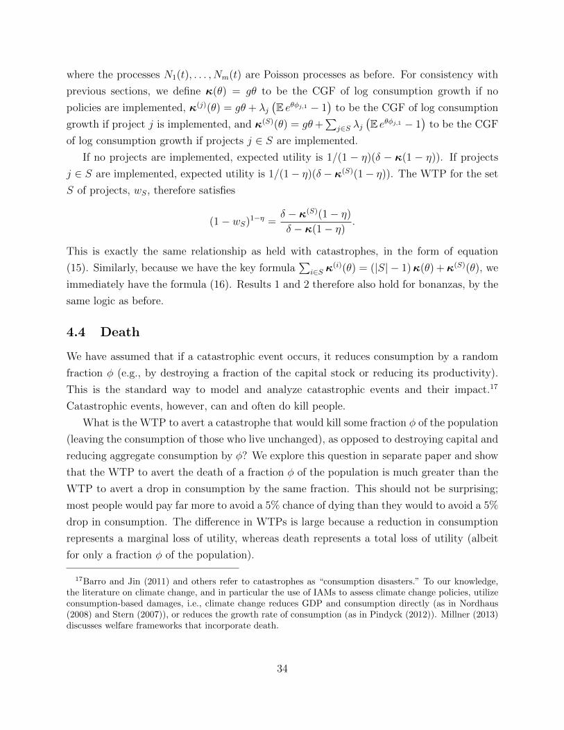
where the processes N1(t), . . . , Nm(t) are Poisson processes as before. For consistency with

previous sections, we define κ(θ) = gθ to be the CGF of log consumption growth if no

policies are implemented, κ(j)(θ) = gθ + λj(E eθφj,1 − 1

)to be the CGF of log consumption

growth if project j is implemented, and κ(S)(θ) = gθ+∑

j∈S λj(E eθφj,1 − 1

)to be the CGF

of log consumption growth if projects j ∈ S are implemented.

If no projects are implemented, expected utility is 1/(1 − η)(δ − κ(1 − η)). If projects

j ∈ S are implemented, expected utility is 1/(1− η)(δ − κ(S)(1− η)). The WTP for the set

S of projects, wS, therefore satisfies

(1− wS)1−η =δ − κ(S)(1− η)

δ − κ(1− η).

This is exactly the same relationship as held with catastrophes, in the form of equation

(15). Similarly, because we have the key formula∑

i∈S κ(i)(θ) = (|S| − 1)κ(θ) +κ(S)(θ), we

immediately have the formula (16). Results 1 and 2 therefore also hold for bonanzas, by the

same logic as before.

4.4 Death

We have assumed that if a catastrophic event occurs, it reduces consumption by a random

fraction φ (e.g., by destroying a fraction of the capital stock or reducing its productivity).

This is the standard way to model and analyze catastrophic events and their impact.17

Catastrophic events, however, can and often do kill people.

What is the WTP to avert a catastrophe that would kill some fraction φ of the population

(leaving the consumption of those who live unchanged), as opposed to destroying capital and

reducing aggregate consumption by φ? We explore this question in separate paper and show

that the WTP to avert the death of a fraction φ of the population is much greater than the

WTP to avert a drop in consumption by the same fraction. This should not be surprising;

most people would pay far more to avoid a 5% chance of dying than they would to avoid a 5%

drop in consumption. The difference in WTPs is large because a reduction in consumption

represents a marginal loss of utility, whereas death represents a total loss of utility (albeit

for only a fraction φ of the population).

17Barro and Jin (2011) and others refer to catastrophes as “consumption disasters.” To our knowledge,the literature on climate change, and in particular the use of IAMs to assess climate change policies, utilizeconsumption-based damages, i.e., climate change reduces GDP and consumption directly (as in Nordhaus(2008) and Stern (2007)), or reduces the growth rate of consumption (as in Pindyck (2012)). Millner (2013)discusses welfare frameworks that incorporate death.

34

The actual difference in WTPs depends on the value of a life lost, which is often proxied

by the “value of a statistical life” (VSL). The VSL is usually defined as the marginal rate

of substitution between wealth (or consumption, or discounted consumption over a lifetime)

and the probability of survival. Thus it is a local measure, and is highly imperfect in that

we would expect an individual or society to be willing to pay much more than the VSL

to avoid certain death. Many studies have estimated the VSL using data on risk-of-death

choices made by individuals, and typically find numbers in the range of 3 to 10 times lifetime

income or consumption. In Martin and Pindyck (2014), we show that using a VSL of 6 times

lifetime consumption implies that the WTP to avoid a probability of death of φ is equal to

the WTP to avoid a drop in consumption of roughly 5φ or more. Some of the catastrophes

that we will consider in the next section involve death, and we will use such a multiple to

translate a φ for death into a welfare-equivalent φ for lost consumption.

5 Some Rough Numbers

This paper is largely theoretical in nature; our objective has been to show that policies

or projects to avert or reduce the likelihood of major catastrophes cannot be analyzed in

isolation, and the problem of deciding which catastrophes should be averted and which

should not is non-trivial. However, it is useful to examine some rough numbers to see how

our framework could be applied in practice. To that end, we examine some of the potential

catastrophes that we believe are important, along with some very rough estimates of the

likelihood, potential impact, and cost of averting each of them.

We assume that the impact of each event is governed by the power distribution (6) for

z = e−φ, so for each type of catastrophe βi is determined from an estimate of E zi. Using

estimates of λi and τi, we set g = δ = .02 and calculate wi, Bi, and Ki for η = 2 and

η = 4. The wi for each catastrophe is calculated taking into account the presence of the

other catastrophes. The estimates of λi, βi, and τi are summarized in Table 1 along with the

calculated values of wi, Bi, and Ki. The last row of the table shows the WTP to avert all

seven catastrophes (w1,...,7 <∑

iwi) and the corresponding benefit and cost in utility terms,

B1,...,7 =∑

iBi and 1 +K1,...,7 =∏

i(1 +Ki). Note that for both values of η, B1,...,7 > K1,...,7,

but as we will see, it is not optimal to avert all seven catastrophes.

The estimates of λi, βi, and τi are explained in Appendix D. For some of the catastrophes

(floods, storms, and earthquakes), the estimates are based on a relatively large amount of

data. For others (e.g., nuclear terrorism), they are based on the subjective estimates of

several authors, and readers may disagree with some of the numbers. As a result, they

35

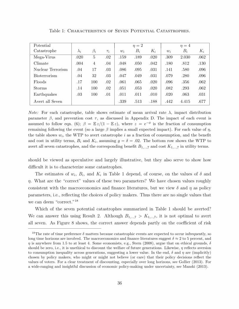
Table 1: Characteristics of Seven Potential Catastrophes.

Potential η = 2 η = 4Catastrophe λi βi τi wi Bi Ki wi Bi Ki

Mega-Virus .020 5 .02 .159 .189 .020 .309 2.030 .062

Climate .004 4 .04 .048 .050 .042 .180 .812 .130

Nuclear Terrorism .04 17 .03 .086 .095 .031 .141 .580 .096

Bioterrorism .04 32 .03 .047 .049 .031 .079 .280 .096

Floods .17 100 .02 .061 .065 .020 .096 .356 .062

Storms .14 100 .02 .051 .053 .020 .082 .293 .062

Earthquakes .03 100 .01 .011 .011 .010 .020 .063 .031

Avert all Seven .339 .513 .188 .442 4.415 .677

Note: For each catastrophe, table shows estimate of mean arrival rate λ, impact distribution

parameter β, and prevention cost τ , as discussed in Appendix D. The impact of each event is

assumed to follow eqn. (6); β = E z/(1 − E z), where z = e−φ is the fraction of consumption

remaining following the event (so a large β implies a small expected impact). For each value of η,

the table shows wi, the WTP to avert catastrophe i as a fraction of consumption, and the benefit

and cost in utility terms, Bi and Ki, assuming g = δ = .02. The bottom row shows the WTP to

avert all seven catastrophes, and the corresponding benefit B1,...,7 and cost K1,...,7 in utility terms.

should be viewed as speculative and largely illustrative, but they also serve to show how

difficult it is to characterize some catastrophes.

The estimates of wi, Bi, and Ki in Table 1 depend, of course, on the values of δ and

η. What are the “correct” values of these two parameters? We have chosen values roughly

consistent with the macroeconomics and finance literatures, but we view δ and η as policy

parameters, i.e., reflecting the choices of policy makers. Thus there are no single values that

we can deem “correct.”18

Which of the seven potential catastrophes summarized in Table 1 should be averted?

We can answer this using Result 2. Although B1,...,7 > K1,...,7, it is not optimal to avert

all seven. As Figure 8 shows, the correct answer depends partly on the coefficient of risk

18The rate of time preference δ matters because catastrophic events are expected to occur infrequently, solong time horizons are involved. The macroeconomics and finance literatures suggest δ ≈ 2 to 5 percent, andη is anywhere from 1.5 to at least 4. Some economists, e.g., Stern (2008), argue that on ethical grounds, δshould be zero, i.e., it is unethical to discount the welfare of future generations. Likewise, η reflects aversionto consumption inequality across generations, suggesting a lower value. In the end, δ and η are (implicitly)chosen by policy makers, who might or might not believe (or care) that their policy decisions reflect thevalues of voters. For a clear treatment of discounting, especially over long horizons, see Gollier (2013). Fora wide-ranging and insightful discussion of economic policy-making under uncertainty, see Manski (2013).

36

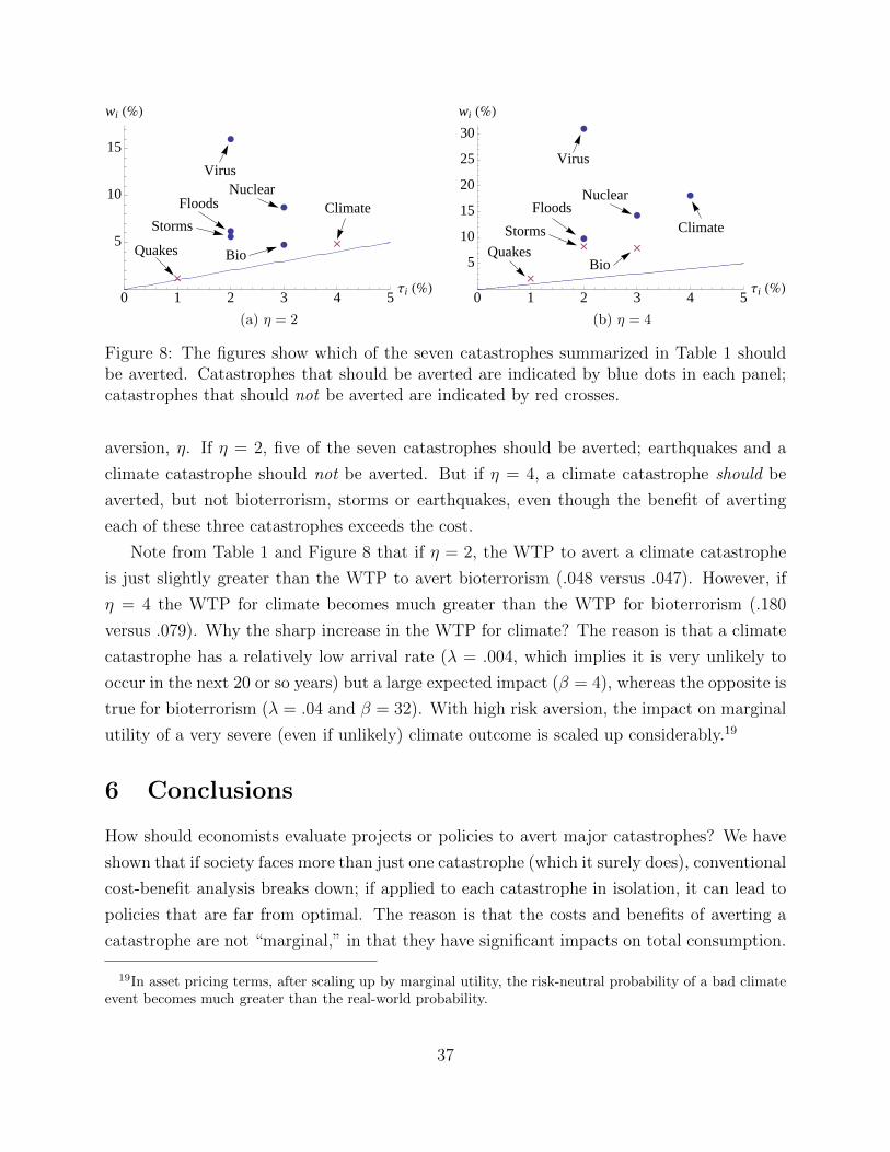
è

è

è

èè

�

�

Quakes

Storms

Floods

Virus

Bio

NuclearClimate

0 1 2 3 4 5Τi H%L

5

10

15

wi H%L

(a) η = 2

è

è

è

è

��

�

Quakes

Storms

Floods

Virus

Bio

Nuclear

Climate

0 1 2 3 4 5Τi H%L

5

10

15

20

25

30

wi H%L

(b) η = 4

Figure 8: The figures show which of the seven catastrophes summarized in Table 1 shouldbe averted. Catastrophes that should be averted are indicated by blue dots in each panel;catastrophes that should not be averted are indicated by red crosses.

aversion, η. If η = 2, five of the seven catastrophes should be averted; earthquakes and a

climate catastrophe should not be averted. But if η = 4, a climate catastrophe should be

averted, but not bioterrorism, storms or earthquakes, even though the benefit of averting

each of these three catastrophes exceeds the cost.

Note from Table 1 and Figure 8 that if η = 2, the WTP to avert a climate catastrophe

is just slightly greater than the WTP to avert bioterrorism (.048 versus .047). However, if

η = 4 the WTP for climate becomes much greater than the WTP for bioterrorism (.180

versus .079). Why the sharp increase in the WTP for climate? The reason is that a climate

catastrophe has a relatively low arrival rate (λ = .004, which implies it is very unlikely to

occur in the next 20 or so years) but a large expected impact (β = 4), whereas the opposite is

true for bioterrorism (λ = .04 and β = 32). With high risk aversion, the impact on marginal

utility of a very severe (even if unlikely) climate outcome is scaled up considerably.19

6 Conclusions

How should economists evaluate projects or policies to avert major catastrophes? We have

shown that if society faces more than just one catastrophe (which it surely does), conventional

cost-benefit analysis breaks down; if applied to each catastrophe in isolation, it can lead to

policies that are far from optimal. The reason is that the costs and benefits of averting a

catastrophe are not “marginal,” in that they have significant impacts on total consumption.

19In asset pricing terms, after scaling up by marginal utility, the risk-neutral probability of a bad climateevent becomes much greater than the real-world probability.

37

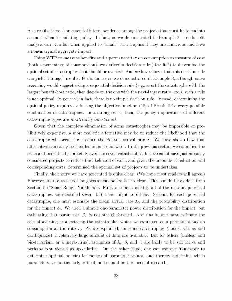
As a result, there is an essential interdependence among the projects that must be taken into

account when formulating policy. In fact, as we demonstrated in Example 2, cost-benefit

analysis can even fail when applied to “small” catastrophes if they are numerous and have

a non-marginal aggregate impact.

Using WTP to measure benefits and a permanent tax on consumption as measure of cost

(both a percentage of consumption), we derived a decision rule (Result 2) to determine the

optimal set of catastrophes that should be averted. And we have shown that this decision rule

can yield “strange” results. For instance, as we demonstrated in Example 3, although naive

reasoning would suggest using a sequential decision rule (e.g., avert the catastrophe with the

largest benefit/cost ratio, then decide on the one with the next-largest ratio, etc.), such a rule

is not optimal. In general, in fact, there is no simple decision rule. Instead, determining the

optimal policy requires evaluating the objective function (18) of Result 2 for every possible

combination of catastrophes. In a strong sense, then, the policy implications of different

catastrophe types are inextricably intertwined.

Given that the complete elimination of some catastrophes may be impossible or pro-

hibitively expensive, a more realistic alternative may be to reduce the likelihood that the

catastrophe will occur, i.e., reduce the Poisson arrival rate λ. We have shown how that

alternative can easily be handled in our framework. In the previous section we examined the

costs and benefits of completely averting seven catastrophes, but we could have just as easily

considered projects to reduce the likelihood of each, and given the amounts of reduction and

corresponding costs, determined the optimal set of projects to be undertaken.

Finally, the theory we have presented is quite clear. (We hope most readers will agree.)

However, its use as a tool for government policy is less clear. This should be evident from

Section 5 (“Some Rough Numbers”). First, one must identify all of the relevant potential

catastrophes; we identified seven, but there might be others. Second, for each potential

catastrophe, one must estimate the mean arrival rate λi, and the probability distribution

for the impact φi. We used a simple one-parameter power distribution for the impact, but

estimating that parameter, βi, is not straightforward. And finally, one must estimate the

cost of averting or alleviating the catastrophe, which we expressed as a permanent tax on

consumption at the rate τi. As we explained, for some catastrophes (floods, storms and

earthquakes), a relatively large amount of data are available. But for others (nuclear and

bio-terrorism, or a mega-virus), estimates of λi, βi and τi are likely to be subjective and

perhaps best viewed as speculative. On the other hand, one can use our framework to

determine optimal policies for ranges of parameter values, and thereby determine which

parameters are particularly critical, and should be the focus of research.

38

Appendix

A. Catastrophe Can Only Occur Once

If a catastrophic event can occur only once, welfare is

V0 = E∫ ∞0

1

1− ηC1−ηt e−δtdt

=1

1− ηE[∫ τ

0

e−ρtdt+

∫ ∞τ

e−φ(1−η)−ρtdt

],

where E denotes the expectation over τ and φ. As before, WTP is defined as the maximum

percentage of consumption, now and throughout the future, that society would give up to

eliminate the possibility of the catastrophe. As before, define ρ = δ + g(η − 1). If society

gives up a fraction w of consumption, net welfare is

V1 = (1− w)1−η∫ ∞0

1

1− ηe−ρtdt.

WTP is then the value w∗ that equates V0 and V1.

To obtain the WTP for eliminating the event, note that welfare if no action is taken is:

V0 =1

1− ηE[∫ T

0

e−ρtdt+ e−φ(1−η)∫ ∞T

e−ρtdt

]=

1

ρ(1− η)E[1 + e−ρT (e−φ(1−η) − 1)

]=

1

ρ(1− η)

[1 +

λ

λ+ ρ

(E e−φ(1−η) − 1

)]=

1

ρ(1− η)

[1 +

λ

λ+ ρ

η − 1

β − η + 1

](1)

If the event is eliminated, welfare net of the fraction w of consumption sacrificed is

V1 =(1− w)1−η

ρ(1− η)(2)

Comparing (1) and (2), the WTP to eliminate the event is:

w∗ = 1−[1 +

λ

λ+ ρ

η − 1

β − η + 1

] 11−η

From this equation, we see that (i) w∗ is an increasing function of the mean arrival rate λ;

(ii) w∗ is an increasing function of the expected impact E(φ), and thus a decreasing function

of the distribution parameter β; and (iii) w∗ is a decreasing function of both the rate of

39

time preference δ and the growth rate g. We would expect w∗ to be higher for an event

that is expected to occur sooner and have a larger expected impact, and lower if either the

rate of time preference or the consumption growth rate is higher. The dependence on η is

ambiguous. Given the growth rate g, a higher value of η implies a lower marginal utility of

future consumption, and thus a lower WTP to avoid a drop in consumption. On the other

hand it also implies a greater sensitivity to uncertainty over future consumption.

As mentioned above, we need β > η − 1. It is easy to see that as η is increased, w∗

approaches 1 as η approaches β + 1. The reason is that the risk-adjusted remaining fraction

of consumption is E((1 − φ)1−η) = β/(β − η + 1). In risk-adjusted terms, the possibility of

a high-φ outcome weighs heavily on expected future welfare, and thus on the WTP.

A few numbers: Suppose β = 2 so the expected loss is Eφ = .33, λ = .05 so the expected

arrival time of the event is ET = 1/λ = 20 years, δ = g = .02, and η = 2. Then w∗ = 0.22.

If instead δ = 0, then w∗ = 0.26. If δ = .02 as before but we increase η to 2.5, w∗ increases

sharply, to 0.60.

It is useful to compare the WTP to avoid this “once-only” event with the WTP when

the event can occur multiple times. Recall that in the latter case the WTP is

w∗m = 1−[1− λ(η − 1)

ρ(β − η + 1)

] 1η−1

.

(The subscript m is added to emphasize that the event can occur multiple times.) Whether

the event can occur only once or repeatedly: (i) w∗ is increasing in the mean arrival rate

λ; (ii) w∗ is increasing in the expected impact E(1 − φ), and thus a decreasing function of

the distribution parameter β; and (iii) w∗ is a decreasing function of both the rate of time

preference δ and the growth rate g. And as expected, w∗m > w∗ for all η > 1, β > η−1, λ > 0.

Some comparisons; for η = 2, g = δ = .02 so ρ = .04, λ = .02 and β = 3 (so E(1−φ) = .75):

• (Base case): w∗ = .143 and w∗m = .250

• λ = .04: w∗ = .200 and w∗m = .500

• λ = .04, β = 2.1: w∗ = .313 and w∗m = .910

In the last example, β is just above the limit (2.0) at which expected utility becomes un-

bounded.

B. The CGF in (2)

We need to calculate ECθ1 . To do so, use the law of iterated expectations:

ECθ1 = E

[E(Cθ

1

∣∣N(1))]

=∞∑m=0

P(N(1) = m)E[eθ(g−

∑N(1)n=1 φn)

∣∣∣N(1) = m].

40

Since N(1) is distributed according to a Poisson distribution with parameter λ,

P(N(1) = m) = e−λλm

m!.

Meanwhile,

E[eθ(g−

∑N(1)n=1 φn)

∣∣∣N(1) = m]

= E[eθ(g−

∑mn=1 φn)

]= eθg

(E e−θφ1

)mbecause the catastrophe sizes φ1, . . . , φm are i.i.d. Thus

ECθ1 =

∞∑m=0

e−λλm

m!eθg(E e−θφ1

)m= e−λ+θg

∞∑m=0

(λE e−θφ1

)mm!

= e−λ+θg exp{λE e−θφ1

}.

Taking logs, κ(θ) = gθ + λ(E e−θφ1 − 1

), as required.

C. Proof of Results 4 and 5

Proof of Result 4. Property (i) follows immediately from (18) and the fact that (1+Bi)/(1+

Ki) > 1, so that we do better by eliminating i than by doing nothing at all. (This does not

imply, however, that it is optimal to avert i itself—there may be even better options.)

Property (ii) follows by contradiction: if j were not included in the set of catastrophes

to be eliminated, then we could increase the objective function in (18) by replacing i with j.

Property (iii) follows because if Bi > Ki, some catastrophe should be averted, by (i).

And now by (ii), we see that catastrophe i should be averted.

To prove that (iv) holds, note first that by Result 3, it is never optimal to avert a

catastrophe with τi ≥ wi. So restrict attention to catastrophes with wi > τi. Then, by

Result 2, we seek to

maxS

1 +∑

i∈S(α1−ηi − 1

)∏i∈S β

1−ηi

,

where αi = 1−wi and βi = 1− τi are fixed and satisfy 0 < αi < βi < 1 for all i. Since βi < 1

and η > 1, the denominator explodes as η →∞. Thus, the problem is equivalent to

maxS

∏i∈S

βη−1i

∑j∈S

α1−ηj ,

or

maxS

∏i∈S

βi

(∑j∈S

α1−ηj

) 1η−1

.

41

Now we use the fact that for arbitrary positive x1, . . . , xN , we have limθ→∞(xθ1 + · · ·+ xθN

) 1θ =

maxi xi. This means that for sufficiently large η, the problem is equivalent to

maxS

(maxk∈S

1

αk

)∏i∈S

βi.

Notice that for a fixed set S, (maxk∈S

1

αk

)∏i∈S

βi ≤ maxk∈S

βkαk,

because βi < 1 for all i. So given a candidate set S, we can increase the objective function

by averting only the catastrophe k ∈ S that maximizes βk/αk. This holds for arbitrary S, so

the unconstrained optimum is achieved by averting only a single catastrophe that maximizes

βk/αk. This is equivalent to the conditions provided in the statement of the result.

Proof of Result 5. With log utility, we can use the property of the CGF that κ′t(0) =

E logCt to write expected utility as

E∫ ∞0

e−δt logCt dt =

∫ ∞0

e−δtκ′t(0) dt = κ′(0)

∫ ∞0

te−δt dt =κ′(0)

δ2.

If we eliminate catastrophes 1 through N costlessly, expected utility is κ(1,...,N)′(0)/δ2.

So WTPs satisfy

log(1− w1,...,N) =κ′(0)− κ(1,...,N)′(0)

δand log(1− wi) =

κ′(0)− κ(i)′(0)

δ. (3)

Exploiting the same relationship between CGFs as before, we find that

N∑i=1

κ′(0)− κ(i)′(0)

δ=

κ′(0)− κ(1,...,N)′(0)

δ,

and soN∑i=1

log(1− wi) = log(1− w1,...,N). (4)

Now, suppose we eliminate catastrophes 1 through N at cost τi (i.e., as before, consump-

tion is multiplied by (1− τi) to eliminate catastrophe i), then expected utility is

E∫ ∞0

e−δt log[C

(1,...,N)t (1− τ1) · · · (1− τN)

]dt =

1

δ2κ(1,...,N)′(0)+

1

δ[log(1− τ1) + · · ·+ log(1− τN)]

where C(1,...,N)t is notation for the consumption process after eliminating catastrophes 1

through N . Using equation (3), this becomes

1

δ2[κ′(0)− δ log(1− w1,...,N)] +

1

δ[log(1− τ1) + · · ·+ log(1− τN)] ,

42

and using (4), this becomes

1

δ2κ′(0) +

1

δ

[log

(1− τ11− w1

)+ · · ·+ log

(1− τN1− wN

)].

This means that the problem is separable: we should eliminate projects i with wi > τi.

D. Catastrophe Characteristics

Here we explain how we arrived at the numbers in Table 1. For catastrophes such as floods,

storms, and earthquakes, a relatively large amount of data were available. For others (e.g.,

nuclear terrorism), there is little or no data, so the numbers are based on the subjective

estimates of several authors. As a result, those numbers should be viewed as speculative and

largely illustrative.

Mega-Viruses: Numerous authors view major pandemics as both likely and having a

catastrophic impact, but do not estimate probabilities of occurrence. Instead, an occurrence

is simply viewed by several authors as “likely.” For a range of possibilities, see Byrne (2008)

and Kilbourne (2008). For detailed discussions of how such mega-viruses could start (and

maybe end), see, e.g., Beardsley (2006) and Enserink (2004). A mega-virus would directly

reduce GDP and consumption by reducing trade, travel, and economic activity worldwide,

but its greatest impact would be the deaths of many people. In related work (Martin and

Pindyck (2014)), we show that the WTP to avert an event that kills a random φ percent

of the population is much larger than the WTP to avert an event that reduces everyone’s

consumption by the same fraction φ.

The last major pandemic to affect developed countries was the Spanish flu of 1918–

1919, which infected roughly 20 percent of the world’s population and killed 3 to 5 percent.

Because populations today have greater mobility (including air travel), a similar virus could

spread more easily. We take the average mortality rate of the next pandemic to be 3.5

percent, which we estimate is equivalent in welfare terms to a roughly 17.5 percent drop in

consumption.20 This corresponds to a value of .825/.175 = 4.7 for β, which we round to 5.

We assume λ = .02, i.e., there is roughly a 20 percent chance of a pandemic occurring in the

next 10 years.

What would be required to avert such an event? There is nothing that can be done

to prevent new viruses from evolving and infecting humans (most likely from an animal

host). If a new virus is extremely virulent and contagious, containment involves (1) the

implementation of systems to identify and isolate infected individuals (e.g., before they

20We use a multiple of 5, which, as discussed in Martin and Pindyck (2014), would apply if we use the“value of a statistical life” (VSL) to represent the value of a life lost, and take the VSL to be six timeslifetime consumption. A great many studies have sought to estimate the VSL using data on risk-of-deathchoices made by individuals, and typically find that the VSL is on the order of 3 to 10 times lifetime incomeor lifetime consumption. See, for example, Viscusi (1993) and Cropper and Sussman (1990).

43

board planes or trains); and (2) the rapid production of a vaccine (which would require

yet-to-be developed technologies, and government investment in a large-scale production

facility). Both of these elements involve substantial ongoing costs, but we are not aware of

any estimates of how large those costs would be. As a best guess, we will assume that those

costs could amount to 2% or more of GDP, and set τ = .02.

Climate: A consensus estimate of the increase in global mean temperature that would

be catastrophic is about 5 to 7◦C. A summary of 22 climate science studies surveyed by

Intergovernmental Panel on Climate Change (2007) puts the probability of this occurring

by the end of the century at around 5 to 10%. Preliminary drafts of the 2014 IPCC report

suggest a somewhat higher probability. Weitzman (2009, 2011) argued that the probability

distribution is fat-tailed, making the actual probability 10% or more. We will use the “pes-

simistic” end of the range and assume that there is a 20% chance that a catastrophe climate

outcome could occur in the next 50 or 60 years, which implies that λ = .004. What would be

the impact of a catastrophic increase in temperature? Estimates of the effective reduction

in (world) GDP from catastrophic warming range from 10% to 30%; we will take the middle

of this range, which puts φ at .20 (so that β = 4).21

What would be the cost of averting a climate catastrophe? Some have argued that this

would require limiting the atmospheric GHG concentration to 450 ppm, and estimates of

the cost of achieving this target vary widely. A starting point would be the GHG emission

reductions mandated by the Kyoto Protocol (which the U.S. never signed). Estimates of the

cost of compliance with the Protocol range from 1% to 3% of GDP.22 Using the middle of

that range (2%) and assuming that stabilizing the GHG concentration at 450 ppm would be

twice as costly as Kyoto gives a cost of τ = .04.

Nuclear Terrorism: Various studies have assessed the likelihood and impact of the

detonation of one or several nuclear weapons (with the yield of the Hiroshima bomb) in

major cities. At the high end, Allison (2004) put the probability of this occurring in the

U.S. in the subsequent ten years at about 50%, which would imply a mean arrival rate

λ = .07. Others put the probability for the subsequent ten years at around 5%, which

implies λ = .005. For a survey, see Ackerman and Potter (2008). We take an average of

these two arrival rates and round it to λ = .04.

What would be the impact? Possibly a million or more deaths in the U.S., which is

0.3% of the population. In welfare terms, this would be equivalent to a roughly 1.5% drop

in consumption. But the main impact would be a shock to the capital stock and GDP

from a reduction in trade and economic activity worldwide, as vast resources would have to

be devoted to averting further events. This could easily result in a 4% drop in GDP and

21See, e.g., Pindyck (2012) and Stern (2007, 2008, 2013).

22See the survey of cost studies by Energy Information Administration (1998) and the more recent countrycost studies surveyed in Intergovernmental Panel on Climate Change (2007).

44

consumption, for a total (effective) drop of 5.5%. This corresponds to β = 17.

The cost of completely averting a nuclear terrorist attack would be considerable. One

element is increased surveillance and intelligence (which presumably is already taking place).

But in addition, we would need to thoroughly inspect all of the containers shipped into the

U.S. daily; currently almost none are inspected. The combined cost of these two activities

could be 3% of GDP, so we set τ = .03.

Bioterrorism: Rough (and largely subjective) estimates of the likelihood of a bioterror-

ist attack and the costs of reducing or eliminating the risks can be found in Nouri and Chyba

(2008) and Lederberg (1999), and references they cite. We will assume that the likelihood of

a bioterrorist attack is about the same as a nuclear attack, and set λ = .04. Bioterrorism is

unlikely to result in large numbers of deaths; instead the major impact would be a shock to

GDP from panic and a reduction in trade and economic activity worldwide. As with a nu-

clear attack, vast resources would have to be devoted to averting further attacks. We assume

that a bio-terrorist attack would be somewhat less disruptive than nuclear terrorist attack,

and estimate that it could result in a 3% drop in GDP and consumption. This implies that

β = .97/.03 = 32.

The cost of averting bioterrorism includes increased surveillance and intelligence (which,

as with nuclear terrorism, is presumably already taking place), but also the development

of and capacity to rapidly produce vaccines and anti-viral agents to counter whatever virus

or other organisms were released. We will assume that the cost of completely averting

bioterrorism is the same as for nuclear terrorism, so τ = .03.

Floods, Storms, and Earthquakes: We make use of the recent study by Cavallo et al.

(2013) of natural disasters and their economic impact. They utilized a data set covering 196

countries over the period 1970 to 2008, which combined World Bank data on real GDP

per capita with data on natural disasters and their impacts from the EM-DAT database.23

Cavallo et al. (2013) estimated the effects of disasters occurring in 196 countries during 1970

to 1999 on the countries’ GDP in the following years. There were 2597 disasters during

1970–2008, out of a total of 39 × 196 = 7664 country-year observations, which implies an

average annual rate of 2597/7664 = .34. Of these disasters, about half were floods, about

40% storms (including hurricanes), and about 10% earthquakes. Thus we set λ = .17, .14,

and .03 for floods, storms, and earthquakes respectively.

These disasters resulted in deaths, but the number was almost always very small relative

to the country’s population. (For example, Hurricane Katrina caused 1833 deaths, which was

less than .001% of the U.S. population.) We therefore ignore the death tolls from these events

and focus on the impact on GDP. Cavallo et al. (2013) found that only the largest disasters

(the 99th percentile in terms of deaths per million people) had a statistically significant

23The EM-DAT database was created by the Centre for Research on the Epidemiology of Disasters at theCatholic University of Louvain, and has data on the occurrence and effects of natural disasters from 1900 tothe present. The data can be accessed at http://www.cred.be/.

45

impact on GDP ten years following the event (reducing GDP by 28% relative to what it

would have been otherwise). But although not statistically significant, smaller disasters

(at the 75th percentile) reduced GDP by 5 to 10%. Assuming that events below the 75th

percentile had no impact, we take the average impact for all three types of disasters to be a

1% drop in consumption, which implies β = 100. Thus floods, storms and earthquakes are

relatively common catastrophes, but have relatively small impacts on average.

Storms cannot be prevented, but their impact can be reduced or completely averted.

This involves relocating coastline homes and other buildings, retrofitting homes, putting

power lines underground, etc. Similar steps would have to be taken to avert the impact of

floods. We assume the cost of completely averting each of these disasters is about 2% of

consumption. The cost of averting the impact of earthquakes should be lower — we assume

1% of consumption — because many buildings in vulnerable areas have already been built to

withstand earthquakes. Thus we set τ = .02 for storms and floods, and .01 for earthquakes.

Other Catastrophic Risks: Much less likely, but certainly catastrophic, events include

nuclear war, gamma ray bursts, an asteroid hitting the Earth, and unforeseen consequences

of nanotechnology. For an overview and very rough estimates of likelihoods and impacts,

see Bostrom and Cirkovic (2008), and see Posner (2004) for a further discussion, including

policy implications. We will ignore these other risks.

46

References

Ackerman, Gary, and William C. Potter. 2008. “Catastrophic Nuclear Terrorism: A

Preventable Peril.” In Global Catastrophic Risks. , ed. Nick Bostrom and Milan Cirkovic.

Oxford University Press.

Allison, Graham. 2004. Nuclear Terrorism: The Ultimate Preventable Catastrophe. Henry

Holt & Company.

Backus, David, Mikhail Chernov, and Ian Martin. 2011. “Disasters Implied by Equity

Index Options.” Journal of Finance, 66(6): 1969–2012.

Barrett, Scott. 2008. “The Incredible Economics of Geoengineering.” Environmental and

Resource Economics, 39: 45–54.

Barrett, Scott. 2009. “The Coming Global Climate-Technology Revolution.” Journal of

Economic Perspectives, 23(2): 53–75.

Barro, Robert J. 2013. “Environmental Protection, Rare Disasters, and Discount Rates.”

National Bureau of Economic Research Working Paper 19258.

Barro, Robert J., and Tao Jin. 2011. “On the Size Distribution of Macroeconomic

Disasters.” Econometrica, 79(5): 1567–1589.

Beardsley, T.M. 2006. “Catastrophe in the Wings?” Bioscience, 56(3): 179–180.

Bostrom, Nick, and Milan Cirkovic, ed. 2008. Global Catastrophic Risks. Oxford Uni-

versity Press.

Byrne, Joseph, ed. 2008. Encyclopedia of Pestilence, Pandemics, and Plagues. Greenwood.

Cavallo, Eduardo, Sebastian Galiani, Ilan Noy, and Juan Pantano. 2013. “Catas-

trophic Natural Disasters and Economic Growth.” Review of Economics and Statistics,

95(5): 1549–1561.

Cropper, Maureen L. 1976. “Regulating Activities with Catastrophic Environmental Ef-

fects.” Journal of Environmental Economics and Management, 3: 160–174.

Cropper, Maureen L., and Frances G. Sussman. 1990. “Valuing Future Risks to Life.”

Journal of Environmental Economics and Management, 19: 160–174.

Energy Information Administration. 1998. “Comparing Cost Estimates for the Kyoto

Protocol.” U.S. Government Report 09-45.

47

Enserink, M. 2004. “Avian Influenza: Catastrophe Waiting in the Wings?” Science,

306(5704): 2016.

Gollier, Christian. 2013. Pricing the Planet’s Future. Princeton University Press.

Gollier, Christian, and John W. Pratt. 1996. “Risk Vulnerability and the Tempering

Effect of Background Risk.” Econometrica, 64(5): 1109–1123.

Greenstone, Michael, Elizabeth Kopits, and Ann Wolverton. 2013. “Developing a

Social Cost of Carbon for Use in U.S. Regulatory Analysis: A Methodology and Interpre-

tation.” Review of Environmental Economics and Policy, 7(1): 23–46.

Interagency Working Group on Social Cost of Carbon. 2010. “Technical Support

Document: Social Cost of Carbon for Regulatory Impact Analysis.” U.S. Government.

Intergovernmental Panel on Climate Change. 2007. Climate Change 2007. Cambridge

University Press.

Kilbourne, Edwin Dennis. 2008. “Plagues and Pandemics: Past, Present, and Future.”

In Global Catastrophic Risks. , ed. Nick Bostrom and Milan Cirkovic. Oxford University

Press.

Kimball, Miles S. 1993. “Standard Risk Aversion.” Econometrica, 61(3): 589–611.

Kousky, Carolyn, Olga Rostapshova, Michael Toman, and Richard Zeckhauser.

2009. “Responding to Threats of Climate Change Mega-Catastrophes.” Resources for the

Future Working Paper 09-45.

Lederberg, Joshua. 1999. Biological Weapons: Limiting the Threat. Cambridge,

MA:M.I.T. Press.

MacCracken, M.C. 2009. “Beyond Mitigation: Potential Options for Counter-Balancing

the Climatic and Environmental Consequences of the Rising Concentrations of Greenhouse

Gases.” The World Bank Working Paper 4938.

Manski, Charles F. 2013. Public Policy in an Uncertain World: Analysis and Decisions.

Harvard University Press.

Martin, Ian. 2008. “Disasters and the Welfare Cost of Uncertainty.” American Economic

Review, 98(2): 74–78.

Martin, Ian. 2013. “Consumption-Based Asset Pricing with Higher Cumulants.” Review of

Economic Studies, 80: 745–773.

48

Martin, Ian W.R., and Robert S. Pindyck. 2014. “Death and Destruction in the

Economics of Catastrophes.” Draft manuscript.

Millner, Antony. 2013. “On Welfare Frameworks and Catastrophic Climate Risks.” Journal

of Environmental Economics and Management, 65: 310–325.

Nordhaus, William D. 2008. A Question of Balance: Weighing the Options on Global

Warming Policies. Yale University Press.

Nouri, Ali, and Christopher F. Chyba. 2008. “Biotechnology and Biosecurity.” In Global

Catastrophic Risks. , ed. Nick Bostrom and Milan Cirkovic. Oxford University Press.

Pindyck, Robert S. 2012. “Uncertain Outcomes and Climate Change Policy.” Journal of

Environmental Economics and Management, 63: 289–303.

Pindyck, Robert S. 2013a. “Climate Change Policy: What Do the Models Tell Us?”

Journal of Economic Literature, 51(3): 860–872.

Pindyck, Robert S. 2013b. “The Climate Policy Dilemma.” Review of Environmental

Economics and Policy, 7(2): 219–237.

Pindyck, Robert S., and Neng Wang. 2013. “The Economic and Policy Consequences

of Catastrophes.” American Economic Journal: Economic Policy, 5(4): 306–339.

Posner, Richard A. 2004. Catastrophe: Risk and Response. New York:Oxford University

Press.

Stern, Nicholas. 2007. The Economics of Climate Change: The Stern Review. Cambridge

University Press.

Stern, Nicholas. 2008. “The Economics of Climate Change.” American Economic Review,

98: 1–37.

Stern, Nicholas. 2013. “The Structure of Economic Modeling of the Potential Impacts

of Climate Change Has Grafted Gross Underestimation onto Already Narrow Science

Models.” Journal of Economic Literature, 51: 838–859.

Sunstein, Cass R. 2007. Worst-Case Scenarios. Harvard University Press.

Viscusi, W. Kip. 1993. “The Value of Risks to Life and Health.” Journal of Economic

Literature, 31(4): 1912–1946.

Weitzman, Martin L. 2009. “On Modeling and Interpreting the Economics of Catastrophic

Climate Change.” Review of Economics and Statistics, 91: 1–19.

49

Weitzman, Martin L. 2011. “Fat-Tailed Uncertainty and the Economics of Climate

Change.” Review of Environmental Economics and Policy, 5(2): 275–292.

Woo, Gordon. 1999. The Mathematics of Natural Catastrophes. London:Imperial College

Press.

50