Embed Size (px)
Citation preview

Combustion Module
AVL FIRE® VERSION 2014


Combustion Module FIRE v2014
AVL LIST GmbH Hans-List-Platz 1, A-8020 Graz, Austria http://www.avl.com AST Local Support Contact: www.avl.com/ast-worldwide
Revision Date Description Document No. A 30-Jun-2008 FIRE v2008 - ICE Physics & Chemistry Users Guide 08.0205.0860 B 15-Apr-2009 FIRE v2009 - ICE Physics & Chemistry Users Guide 08.0205.2009 C 30-Sep-2009 FIRE v2009.1 - ICE Physics & Chemistry Users Guide 08.0205.2009.1 D 30-Nov-2010 FIRE v2010 - ICE Physics & Chemistry Users Guide 08.0205.2010 E 14-Oct-2011 FIRE v2011 – Combustion / Emission Module 08.0205.2011 F 30-Apr-2012 FIRE v2011.1 – Combustion / Emission Module 08.0205.2011.1 G 28-Feb-2013 FIRE v2013 – Combustion Module 08.0205.2013 H 30-Sept-2014 FIRE v2014 – Combustion Module 08.0205.2014
Copyright © 2014, AVL
All rights reserved. No part of this publication may be reproduced, transmitted, transcribed, stored in a retrieval system or translated into any language or computer language, in any form or by any means, electronic, mechanical, magnetic, optical, chemical, manual or otherwise, without prior written consent of AVL.
This document describes how to run the FIRE software. It does not attempt to discuss all the concepts of computational fluid dynamics required to obtain successful solutions. It is the user’s responsibility to determine if he/she has sufficient knowledge and understanding of fluid dynamics to apply this software appropriately.
This software and document are distributed solely on an "as is" basis. The entire risk as to their quality and performance is with the user. Should either the software or this document prove defective, the user assumes the entire cost of all necessary servicing, repair, or correction. AVL and its distributors will not be liable for direct, indirect, incidental, or consequential damages resulting from any defect in the software or this document, even if they have been advised of the possibility of such damage.
FIRE® is a registered trademark of AVL LIST. FIRE® will be referred as FIRE in this manual.
All mentioned trademarks and registered trademarks are owned by the corresponding owners.

Combustion Module FIRE v2014
AST.08.0205.2014 – 30-Sept-2014 i
Table of Contents 1. Introduction _____________________________________________________ 1-1
1.1. Symbols _____________________________________________________________________ 1-1 1.2. Configurations _______________________________________________________________ 1-1
2. Overview ________________________________________________________ 2-1 2.1. Spray/Combustion Interaction _________________________________________________ 2-2 2.2. Activation and Handling of the Combustion Module ______________________________ 2-2
3. Theoretical Background _________________________________________ 3-1 3.1. Nomenclature ________________________________________________________________ 3-1
3.1.1. Roman Characters ________________________________________________________ 3-1 3.1.2. Greek Characters _________________________________________________________ 3-3 3.1.3. Subscripts _______________________________________________________________ 3-4 3.1.4. Superscripts ______________________________________________________________ 3-6
3.2. Combustion Models ___________________________________________________________ 3-6 3.2.1. High Temperature Oxidation Scheme _______________________________________ 3-6 3.2.2. Turbulence Controlled Combustion Model ___________________________________ 3-6 3.2.3. Turbulent Flame Speed Closure Combustion Model ___________________________ 3-7 3.2.4. Coherent Flame Model ____________________________________________________ 3-9
3.2.4.1. CFM-2A Model ________________________________________________________ 3-9 3.2.4.2. MCFM Model ________________________________________________________ 3-12 3.2.4.3. ECFM Model ________________________________________________________ 3-14 3.2.4.4. ECFM-3Z Model _____________________________________________________ 3-32
3.2.5. Probability Density Function Approach ____________________________________ 3-41 3.2.5.1. PDF Transport Equation______________________________________________ 3-41 3.2.5.2. Monte Carlo Simulation _______________________________________________ 3-43
3.2.6. Characteristic Timescale Model ____________________________________________ 3-45 3.2.7. Steady Combustion Model ________________________________________________ 3-46 3.2.8. Multi-Species Chemically Reacting Flows ___________________________________ 3-47
3.2.8.1. Hydrocarbon Auto-Ignition Mechanism _________________________________ 3-47 3.2.8.2. AnB Knock-Prediction Model __________________________________________ 3-49 3.2.8.3. Empirical Knock Model _______________________________________________ 3-51
3.2.9. Flame Tracking Particle Model ____________________________________________ 3-52 3.2.9.1. Basic Concept ________________________________________________________ 3-52 3.2.9.2. Flame Tracking Method _______________________________________________ 3-52 3.2.9.3. Particle Method ______________________________________________________ 3-55 3.2.9.4. Spark Ignition Modeling ______________________________________________ 3-56
3.3. References __________________________________________________________________ 3-58 3.4. Related Publications _________________________________________________________ 3-61
4. Combustion Input Data __________________________________________ 4-1 4.1. Control ______________________________________________________________________ 4-1 4.2. Combustion Models ___________________________________________________________ 4-1
4.2.1. Eddy Breakup Model ______________________________________________________ 4-2
FIRE v2014 Combustion Module
ii AST. 08.0205.2014 - 30-Sept-2014
4.2.1.1. Model Constants ______________________________________________________ 4-3 4.2.1.2. Time Scale ___________________________________________________________ 4-3
4.2.2. Turbulent Flame Speed Closure Model ______________________________________ 4-4 4.2.2.1. Model Constants ______________________________________________________ 4-5
4.2.3. Coherent Flame Model ____________________________________________________ 4-6 4.2.3.1. Time Scale __________________________________________________________ 4-10 4.2.3.2. ECFM-3Z ___________________________________________________________ 4-11
4.2.4. PDF Model ______________________________________________________________ 4-14 4.2.4.1. Rate Coefficient Treatment ____________________________________________ 4-15 4.2.4.2. Time Scale __________________________________________________________ 4-16
4.2.5. Characteristic Timescale Model ____________________________________________ 4-17 4.2.5.1. Model Constants _____________________________________________________ 4-18 4.2.5.2. Time Scale __________________________________________________________ 4-18
4.2.6. Steady Combustion Model ________________________________________________ 4-19 4.2.6.1. Model Constants _____________________________________________________ 4-19
4.2.7. Flame Tracking Particle Model ____________________________________________ 4-20 4.2.7.1. Model Constants _____________________________________________________ 4-21
4.2.8. User Defined Reaction Rate _______________________________________________ 4-22 4.2.9. Time Dependent Activation of Combustion _________________________________ 4-22
4.2.9.1. Combustion Models __________________________________________________ 4-22 4.2.9.2. Auto Ignition Models _________________________________________________ 4-23
4.3. Ignition Models _____________________________________________________________ 4-23 4.3.1. Spark Ignition ___________________________________________________________ 4-23 4.3.2. Auto Ignition ____________________________________________________________ 4-27
4.3.2.1. Diesel _______________________________________________________________ 4-27 4.3.2.2. Diesel_MIL __________________________________________________________ 4-28 4.3.2.3. HCCI _______________________________________________________________ 4-28 4.3.2.4. Knock ______________________________________________________________ 4-29 4.3.2.5. AnB Knock __________________________________________________________ 4-29 4.3.2.6. Empirical Knock Model _______________________________________________ 4-30 4.3.2.7. Diesel Ignited Gas Engine Model _______________________________________ 4-31
4.4. 2D Results __________________________________________________________________ 4-32 4.4.1. General Information _____________________________________________________ 4-32 4.4.2. Auto Ignition Models _____________________________________________________ 4-33
4.5. 3D Results __________________________________________________________________ 4-33 4.5.1. General Information _____________________________________________________ 4-34 4.5.2. CFM Models ____________________________________________________________ 4-36 4.5.3. Auto Ignition Models _____________________________________________________ 4-36 4.5.4. Optional Output from Knock Models _______________________________________ 4-37
4.5.4.1. Knock ______________________________________________________________ 4-37 4.5.4.2. AnB Knock __________________________________________________________ 4-37
Combustion Module FIRE v2014
AST.08.0205.2014 – 30-Sept-2014 iii
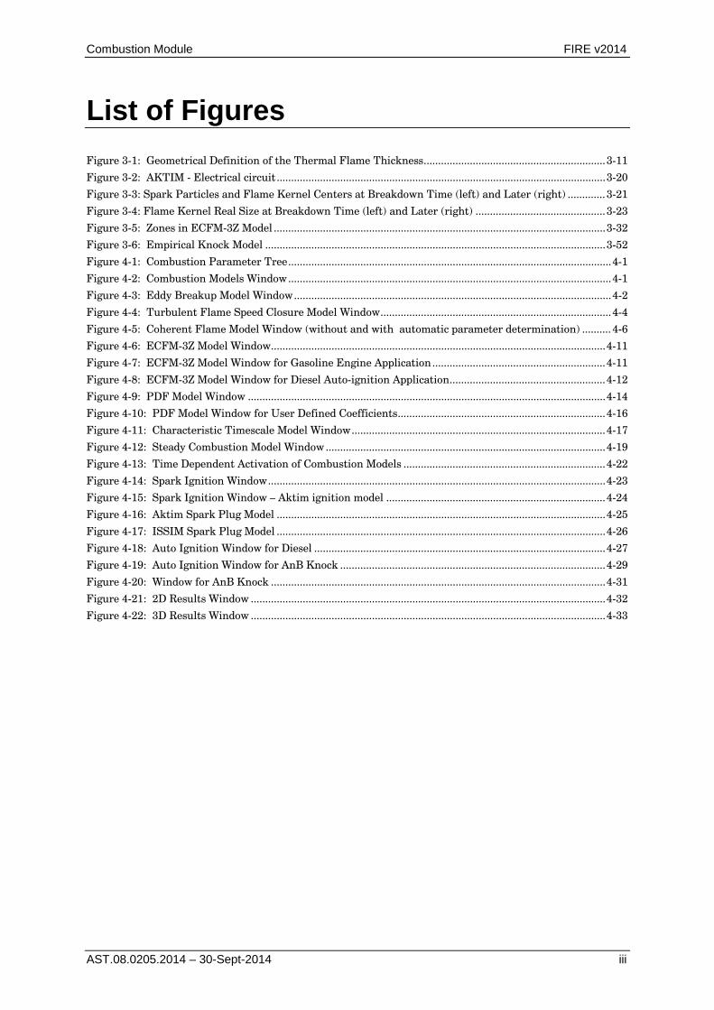
List of Figures Figure 3-1: Geometrical Definition of the Thermal Flame Thickness ............................................................... 3-11 Figure 3-2: AKTIM - Electrical circuit .................................................................................................................. 3-20 Figure 3-3: Spark Particles and Flame Kernel Centers at Breakdown Time (left) and Later (right) ............. 3-21 Figure 3-4: Flame Kernel Real Size at Breakdown Time (left) and Later (right) ............................................. 3-23 Figure 3-5: Zones in ECFM-3Z Model ................................................................................................................... 3-32 Figure 3-6: Empirical Knock Model ...................................................................................................................... 3-52 Figure 4-1: Combustion Parameter Tree ................................................................................................................ 4-1 Figure 4-2: Combustion Models Window ................................................................................................................ 4-1 Figure 4-3: Eddy Breakup Model Window .............................................................................................................. 4-2 Figure 4-4: Turbulent Flame Speed Closure Model Window ................................................................................ 4-4 Figure 4-5: Coherent Flame Model Window (without and with automatic parameter determination) .......... 4-6 Figure 4-6: ECFM-3Z Model Window .................................................................................................................... 4-11 Figure 4-7: ECFM-3Z Model Window for Gasoline Engine Application ............................................................ 4-11 Figure 4-8: ECFM-3Z Model Window for Diesel Auto-ignition Application ...................................................... 4-12 Figure 4-9: PDF Model Window ............................................................................................................................ 4-14 Figure 4-10: PDF Model Window for User Defined Coefficients ........................................................................ 4-16 Figure 4-11: Characteristic Timescale Model Window ........................................................................................ 4-17 Figure 4-12: Steady Combustion Model Window ................................................................................................. 4-19 Figure 4-13: Time Dependent Activation of Combustion Models ...................................................................... 4-22 Figure 4-14: Spark Ignition Window ..................................................................................................................... 4-23 Figure 4-15: Spark Ignition Window – Aktim ignition model ............................................................................ 4-24 Figure 4-16: Aktim Spark Plug Model .................................................................................................................. 4-25 Figure 4-17: ISSIM Spark Plug Model .................................................................................................................. 4-26 Figure 4-18: Auto Ignition Window for Diesel ..................................................................................................... 4-27 Figure 4-19: Auto Ignition Window for AnB Knock ............................................................................................ 4-29 Figure 4-20: Window for AnB Knock .................................................................................................................... 4-31 Figure 4-21: 2D Results Window ........................................................................................................................... 4-32 Figure 4-22: 3D Results Window ........................................................................................................................... 4-33

Combustion Module FIRE v2014
30-Sept-2014 1-1
1. INTRODUCTION This manual describes the usage, files and the theoretical background of the FIRE Combustion Module.
1.1. Symbols The following symbols are used throughout this manual. Safety warnings must be strictly observed during operation and service of the system or its components.
Caution: Cautions describe conditions, practices or procedures which could result in damage to, or destruction of data if not strictly observed or remedied.
Note: Notes provide important supplementary information.
Convention Meaning
Italics For emphasis, to introduce a new term.
monospace To indicate a command, a program or a file name, messages, input / output on a screen, file contents or object names.
MenuOpt A MenuOpt font is used for the names of menu options, submenus and screen buttons.
1.2. Configurations Software configurations described in this manual were in effect on the publication date of this manual. It is the user’s responsibility to verify the configuration of the equipment before applying procedures in this manual.

Combustion Module FIRE v2014
30-Sept-2014 2-1
2. OVERVIEW The FIRE Combustion Module enables the calculation of species transport/mixing phenomena and the simulation of combustion in internal combustion engines and technical combustion devices under premixed, partially premixed and/or non-premixed conditions.
Chemical kinetic effects are accounted for by different single-step and multi-step combustion models for the treatment of the high temperature oxidation processes in flames. For the simulation of the auto-ignition behavior of hydrocarbon fuels also several models are available which can be combined with the high temperature reaction schemes in order to form a simulation chain for Diesel auto-ignition.
A knock model is available for the description of knocking processes considering fuel consumption and heat formation at the knock locations. This knock model can be currently activated only in the case of CFM combustion activation and is mainly constructed for the ECFM but can also be used for the other CFM.
A further knock model is available based on an empirical approach considering no fuel consumption and heat formation at knock locations. In this model local volumes clockwise arranged are determined giving a knock criteria for each segment based on different parameters such as temperature, fuel mass fraction, EGR, etc. This empirical knock model can be used for all combustion models.
The influence of turbulence on the mean rate of reaction may be treated by five different types of combustion models of different levels of complexity. The choice depends on the application case under consideration and the purpose of the numerical simulation.
The first model is based on the ideas of the eddy dissipation concept, which assumes that the mean turbulent reaction rate is determined by the intermixing of cold reactants with hot combustion products.
The second model is a turbulent flame speed closure model determining the mean reaction rate which is based upon an approach depending on parameters of the turbulence such as turbulence intensity and length scale, and of the flame structure like flame speed and thickness, respectively.
The third combustion model is based on the flamelet assumption, i.e. the turbulent flame brush should be composed by an ensemble of laminar flamelets. The length and time scales in the reaction zone are assumed to be smaller than the characteristic turbulent length and time scales, respectively. This model consists of several sub-models including also one for the complete description of the Diesel auto-ignition and combustion process.
The fourth model adopts the Probability Density Function (PDF) approach. This approach fully accounts for the simultaneous effects of both finite rate chemistry and turbulence, thus obviating the need for any prior assumptions as to whether one or the other of the two processes determines the mean rate of reaction.
The fifth model is the Characteristic Timescale Model which takes into account a laminar and a turbulent time scale. The laminar time scale considers the slower chemical reaction rates especially at the beginning of the combustion. The turbulent time scale gives the influence of the turbulent motion to the reaction rate.
A separate model is available for the description of steady combustion processes especially in burners and furnaces.

FIRE v2014 Combustion Module
2-2 30-Sept-2014
2.1. Spray/Combustion Interaction In combination with the FIRE Spray Model, the FIRE Combustion Module enables the calculation of spray combustion processes in direct injection engines. Under these conditions, mixture formation and combustion are simultaneous processes exhibiting a significant degree of interaction and interdependence.
A successful combustion calculation under these conditions relies very much on the accuracy of the spatial and temporal spray vapor evolution characteristics. The use of droplet break-up models with suitably adjusted model parameters is highly recommended for this type of application.
At present, the WAVE breakup model is recommended for simulation of spray combustion phenomena in Diesel engines, with the model constants C1 and C2 set to 0.61 and 12.0 - 30.0, respectively (for more details please refer to the Spray Manual).
2.2. Activation and Handling of the Combustion Module The characteristic features of the turbulent combustion process in a practical device (i.e. the temporal variation of the heat release rate, the turbulent flame speed, or the behavior of the flow-flame interaction) strongly depend on application case-specific physical and chemical (fuel type) parameters. They also strongly depend on parameters such as the location of the ignition device, the ignition timing and the spark duration. All required information is specified in the .ssf-file.
The FIRE Combustion Module is activated in the Solver GUI of the FIRE Workflow Manager.
Combustion Module FIRE v2014
30-Sept-2014 3-1
3. THEORETICAL BACKGROUND
3.1. Nomenclature
3.1.1. Roman Characters q heat release rate
R radical pool
r fuel consumption rate
w mean turbulent reaction rate
a1, a2, a3, a4 stoichiometric relations
A pre-exponential factor; constant; air zone; spark strain
B constant; branching agent
Bl Blint-number
c reaction progress variable
cp specific heat capacity at constant pressure
cv specific heat capacity at constant volume
C carbon atom; correction function; curvature term
C1, C2, C3 turbulence model constants
Cfu, CPr combustion model constants
Cm mixing rate constant
CnHmOl hydrocarbon fuel
CO carbon monoxide
CO2 carbon dioxide
d distance
D current density at electrode surface
dis discharge coefficient
E energy
Ea activation energy
f mixture fraction
fn mixture fraction of maximum nucleation
fu fuel

FIRE v2014 Combustion Module
3-2 30-Sept-2014
F fuel zone; function
Fc Correction function
g residual gas mass fraction
G deformation gradient tensor; constant
h enthalpy; heat transfer coefficient
H hydrogen atom
H2 molecular hydrogen
H2O water
i electrical circuit
I inerts
J Jacobian determinant
k turbulence kinetic energy; reaction rate
K flame stretch
Ka Karlovitz-number
l number of oxygen atoms; integral length scale
l length
L inductance
m mass; number of hydrogen atoms
min minimum value of operator
M molecular weight; mixed zone
n number of carbon atoms; number of particles
N ensemble of notional particles; atomic nitrogen
N2 nitrogen
NO nitrogen monoxide
O atomic oxygen
O2 oxygen
OH hydroxyl radical
p probability density function; pressure
P Production term
Pr Prandtl-number
Q intermediate products; power; heat loss
Qh combustion heat release per fuel mass unit
R universal gas constant; radius

Combustion Module FIRE v2014
30-Sept-2014 3-3
egr residual gas
s chemical reaction term
S stoichiometric oxygen requirement; source term; surface; flame velocity; strain term
Sc Schmidt-number
T temperature; tracer; turbulent; transport term
t time
u velocity
V volume; voltage
x Distance; spark co-ordinates
y mass fraction
Ze Zeldovich-number
3.1.2. Greek Characters ∂ partial derivative
σ n nucleation variance
σ Pr , σ Sc Prandtl number, Schmidt number
∆ Increment; filter size
Φ particle property
Γ diffusion coefficient; ITNFS function
∑ turbulent flame surface density
α , β CFM constants
δ Kronecker delta; flame thickness
ε dissipation rate
φ generalized scalar quantity; equivalence ratio
γ Jacobian factors; function
κ isentropic exponent
λ air excess ratio
µ dynamic viscosity
ρ density
τ time scale
υ viscosity; stoichiometric coefficient
π pi-number
FIRE v2014 Combustion Module
3-4 30-Sept-2014
Ξ folding factor
∇ gradient
ω turbulent frequency; reaction rate; fuel consumption rate
ζηξ ,, transformed coordinate system
3.1.3. Subscripts α index for chemical species; stoichiometric
function
∞ maximum
a annihilation; activation
af anode fall
AI auto-ignition
arc spark arc
b burned; backward; branching
bd breakdown
c convention; combustible; chemical; convection; critical
cf cathode fall
crit critical
curv curvature
CO2 carbon dioxide
d diffusion
e electrical
eff effective
egr residual gas
evap evaporation
f forward
fr fresh
fl flame
fu fuel
FP flame propagation
g surface growth; exhaust gas
gc gas column
Combustion Module FIRE v2014
30-Sept-2014 3-5
H2O water
i Species; intermediate
ie Inner-electrode
ign ignition
i, j, l, r indices
k Kolmogorov
l laminar
lam laminar
m mixing
mean mean
min minimum
min minimum
mix mixed
n nucleation; number of atoms
N2 nitrogen
o oxidation
O2 oxygen
p precursor
pr products
prop propagation
r reaction
s secondary
seg segment
spk spark
st stoichiometric
str strain
S soot
t turbulent; termination
tot total
u unburned; universal
w wall
∑ flame surface density
0 initial
FIRE v2014 Combustion Module
3-6 30-Sept-2014
3.1.4. Superscripts
0 initial
¯ ensemble-averaged
~ density weighted ensemble-averaged
",' fluctuating component
[ ] concentration; dimension
3.2. Combustion Models This section describes the theoretical background of the FIRE combustion module developed for the simulation of species transport, ignition and turbulent combustion of gaseous mixtures of hydrocarbon fuel, air, and residual (exhaust) gas.
The determination of mean chemical reaction rates represents a central problem in the numerical simulation of chemical kinetic processes. This is because they appear to be highly non-linear functions of the local values of temperature and species concentrations.
Although it is desirable to use detailed reaction mechanisms, available computational resources are inadequate to manage thousands of elementary reactions with hundreds of participating species. This is due to the fact that for each species considered in the reaction mechanism, an additional conservation equation must be solved.
3.2.1. High Temperature Oxidation Scheme The complex oxidation process of a hydrocarbon fuel with air occurring during the turbulent combustion process is in most cases expressed in accordance with the current practice ([3.1]; [3.2]) by a single step irreversible reaction of the form:
( ) ( ) 2432423
2221kmn
N aa1OHaCOa kg S1N aOa kg SOHC kg 1
−−+++→++
(3.1)
Refer to the Species Transport Manual for the coefficients a1 … a4 and S.
Some of the models (e.g. the ECFM) are based on more complex oxidation schemes which take more reaction steps and also some equilibrium reactions into account.
3.2.2. Turbulence Controlled Combustion Model One of the combustion models available in FIRE is of the turbulent mixing controlled type, as described by Magnussen and Hjertager [3.37]. This model assumes that in premixed turbulent flames, the reactants (fuel and oxygen) are contained in the same eddies and are separated from eddies containing hot combustion products. The chemical reactions usually have time scales that are very short compared to the characteristics of the turbulent transport processes. Thus, it can be assumed that the rate of combustion is determined by the rate of intermixing on a molecular scale of the eddies containing reactants and those containing hot products, in other words by the rate of dissipation of these eddies. The attractive feature of this model is that it does not call for predictions of fluctuations of reacting species.

Combustion Module FIRE v2014
30-Sept-2014 3-7
The mean reaction rate can thus be written in accordance with [3.37]
+ρ
τ=ρ
S1y C,
Sy,yminCr PrPrOx
fuR
fufu (3.2)
The first two terms of the “minimum value of” operator “min(...)” simply determine whether fuel or oxygen is present in limiting quantity, and the third term is a reaction probability which ensures that the flame is not spread in the absence of hot products. Cfu and Cpr are empirical coefficients and τR is the turbulent mixing time scale for reaction.
The value of the empirical coefficient Cfu has been shown to depend on turbulence and fuel parameters ([3.8]; [3.11]). Hence, Cfu requires adjustment with respect to the experimental combustion data for the case under investigation (for engines, the global rate of fuel mass fraction burnt).
3.2.3. Turbulent Flame Speed Closure Combustion Model For the simulation of homogeneously/inhomogeneously premixed combustion processes in SI engines, a turbulent flame speed closure model (TFSCM) is available in FIRE. The kernel of this model is the determination of the reaction rate based on an approach depending on parameters of turbulence, i.e. turbulence intensity and turbulent length scale, and of flame structure like the flame thickness and flame speed, respectively. The reaction rate can be determined by two different mechanisms via:
• Auto-ignition and
• Flame propagation scheme
The auto-ignition scheme is described by an Arrhenius approach and the flame propagation mechanism depends mainly on the turbulent flame speed. The larger reaction rate of these two mechanisms is the dominant one. Hence, the fuel reaction rate ωfuel can be described using a maximum operator via:
furρ = maxAuto-ignition ωAI, Flame Propagation ωFP (3.3)
The first scheme is only constructed for air/fuel equivalence ratios from 1.5 up to 2.0 and for pressure levels between 30 and 120 [bar], respectively. The auto-ignition reaction rate ωAI can be written as:
−ρ=ω
TTaexpTyya 54
2
32 aaO
afuel
a1AI (3.4)
where a1 to a5 are empirical coefficients and Ta is the activation temperature.
The reaction rate ωFP of the flame propagation mechanism, the second one in this model, can be written as the product of the gas density, the turbulent burning velocity St and the fuel mass fraction gradient ∇yfu via:
fuelTFP yS ∇ρ=ω (3.5)
This approach was initially constructed for homogeneously premixed combustion phenomena. In order to apply this model also for inhomogeneous charge processes, changes were made concerning the determination of this reaction rate.
FIRE v2014 Combustion Module
3-8 30-Sept-2014
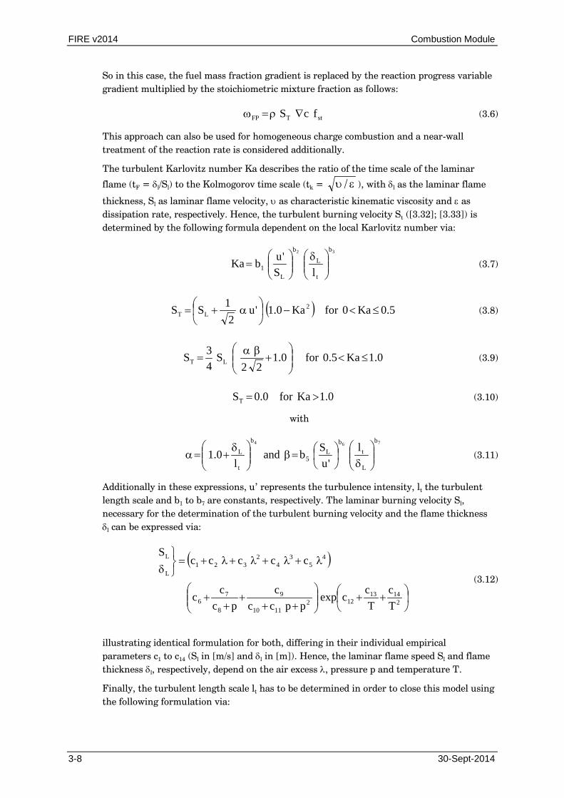
So in this case, the fuel mass fraction gradient is replaced by the reaction progress variable gradient multiplied by the stoichiometric mixture fraction as follows:
stTFP f cS ∇ρ=ω (3.6)
This approach can also be used for homogeneous charge combustion and a near-wall treatment of the reaction rate is considered additionally.
The turbulent Karlovitz number Ka describes the ratio of the time scale of the laminar
flame (tF = δl/Sl) to the Kolmogorov time scale (tk = ευ / ), with δl as the laminar flame
thickness, Sl as laminar flame velocity, υ as characteristic kinematic viscosity and ε as dissipation rate, respectively. Hence, the turbulent burning velocity St ([3.32]; [3.33]) is determined by the following formula dependent on the local Karlovitz number via:
32 b
t
L
b
L1 lS
'ubKa
δ
= (3.7)
( ) 5.0Ka0forKa0.1'u2
1SS 2LT ≤<−
α+= (3.8)
0.1Ka5.0for0.122
S43S LT ≤<
+
βα= (3.9)
0.1Kafor0.0ST >= (3.10)
with
764 b
L
tb
L5
b
t
L l'u
Sbandl
0.1
δ
=β
δ+=α (3.11)
Additionally in these expressions, u’ represents the turbulence intensity, lt the turbulent length scale and b1 to b7 are constants, respectively. The laminar burning velocity Sl, necessary for the determination of the turbulent burning velocity and the flame thickness δl can be expressed via:
( )
++
++
++
+
λ+λ+λ+λ+=
δ
21413
1221110
9
8
76
45
34
2321
L
L
Tc
Tccexp
ppccc
pccc
cccccS
(3.12)
illustrating identical formulation for both, differing in their individual empirical parameters c1 to c14 (Sl in [m/s] and δl in [m]). Hence, the laminar flame speed Sl and flame thickness δl, respectively, depend on the air excess λ, pressure p and temperature T.
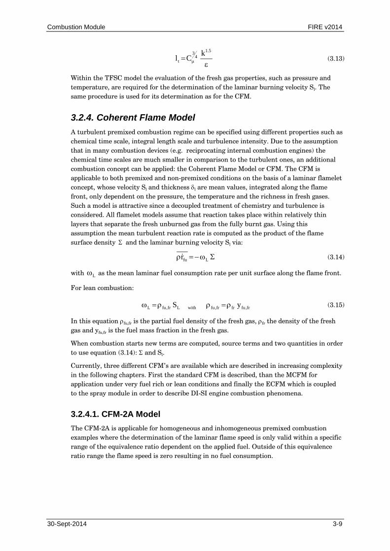
Finally, the turbulent length scale lt has to be determined in order to close this model using the following formulation via:
Combustion Module FIRE v2014
30-Sept-2014 3-9
ε
= µ
5.14
3
tkCl (3.13)
Within the TFSC model the evaluation of the fresh gas properties, such as pressure and temperature, are required for the determination of the laminar burning velocity Sl. The same procedure is used for its determination as for the CFM.
3.2.4. Coherent Flame Model A turbulent premixed combustion regime can be specified using different properties such as chemical time scale, integral length scale and turbulence intensity. Due to the assumption that in many combustion devices (e.g. reciprocating internal combustion engines) the chemical time scales are much smaller in comparison to the turbulent ones, an additional combustion concept can be applied: the Coherent Flame Model or CFM. The CFM is applicable to both premixed and non-premixed conditions on the basis of a laminar flamelet concept, whose velocity Sl and thickness δl are mean values, integrated along the flame front, only dependent on the pressure, the temperature and the richness in fresh gases. Such a model is attractive since a decoupled treatment of chemistry and turbulence is considered. All flamelet models assume that reaction takes place within relatively thin layers that separate the fresh unburned gas from the fully burnt gas. Using this assumption the mean turbulent reaction rate is computed as the product of the flame surface density Σ and the laminar burning velocity Sl via:
Σω−=ρ Lfur (3.14)
with Lω as the mean laminar fuel consumption rate per unit surface along the flame front.
For lean combustion:
fr,fufrfr,fuwithLfr,fuL yS ρ=ρρ=ω (3.15)
In this equation ρfu,fr is the partial fuel density of the fresh gas, ρfr the density of the fresh gas and yfu,fr is the fuel mass fraction in the fresh gas.
When combustion starts new terms are computed, source terms and two quantities in order to use equation (3.14): Σ and Sl.
Currently, three different CFM’s are available which are described in increasing complexity in the following chapters. First the standard CFM is described, than the MCFM for application under very fuel rich or lean conditions and finally the ECFM which is coupled to the spray module in order to describe DI-SI engine combustion phenomena.
3.2.4.1. CFM-2A Model The CFM-2A is applicable for homogeneous and inhomogeneous premixed combustion examples where the determination of the laminar flame speed is only valid within a specific range of the equivalence ratio dependent on the applied fuel. Outside of this equivalence ratio range the flame speed is zero resulting in no fuel consumption.
FIRE v2014 Combustion Module
3-10 30-Sept-2014
3.2.4.1.1. Evolution of Turbulent Flame Surface Density The following equation is solved for the flame surface density Σ ([3.10];[3.15]):
( ) LAMagj
t
jj
j
SSSSxx
uxt
+−==
∂Σ∂
∂∂
−Σ∂
∂+
∂Σ∂
ΣΣσ
ν (3.16)
with Σ as the turbulent flame surface density (the flame area per unit volume), σΣ is the turbulent Schmidt number, νt is the turbulent kinematic viscosity, Sg is the production of the flame surface by turbulent rate of strain and Sa is the annihilation of flame surface due to reactants consumption:
with 2
fu
Lfr,fuaeffg
SSandKS Σ
ρρ
β=Σα= (3.17)
where Keff is the mean stretch rate of the flame, Sa is written for the case of lean combustion but equivalent equation is obtained for rich conditions by replacing the fuel mass fraction by the oxidant mass fraction.
SLAM is the contribution of laminar combustion to the generation of flame surface density. The term considers three different effects:
SCPSLAM ++= (3.18)
showing the contribution of propagation, curvature and straining to the flame propagation as described later.
3.2.4.1.2. Stretching and Quenching of Flamelets Stretching and quenching of flame surface density in term SΣ of equation (3.16) is treated through the Intermittent Turbulence Net Flame Stretch- or ITNFS-model [3.39] describing the interaction between one vortex and a flame front through direct simulation [3.42]. By extending it to a complete turbulent flow, it is assumed that the total effect of all turbulent fluctuations can be deduced from the behavior of each scale. The production of flame surface density comes essentially from the turbulent net flame stretch. The flame stretch is written as the large scale characteristic strain ε/k corrected by a function Ct, which accounts for the size of turbulence scales, viscous and transient effects [3.40]. Ct is a function of turbulence parameters and laminar flame characteristics. Hence, the turbulent flame stretch Kt is dependent upon the turbulent to laminar flame velocity and length ratios: Ct = f(u’/Sl , lt/δl). u’ is the RMS turbulence velocity, lt the integral turbulent length scale and δl the laminar flame thickness.
Kteff CkKK ε== (3.19)
Kt is a very important property since it influences the source term for the flame surface and therefore the mean turbulent reaction rate. α and β are arbitrary tuning constants used in CFM.

Combustion Module FIRE v2014
30-Sept-2014 3-11
3.2.4.1.3. Laminar Flame Speed The laminar flame speed is supposed to depend only upon the local pressure, the ‘fresh gas’ temperature Tfr from equation (3.25) and the local unburned fuel/air equivalence ratio φfr.
If the correlation of Metghalchi and Keck [3.41] is chosen in the GUI, the following empirical relations (valid for premixed combustion at high pressure and temperature) are applied:
( )21 a
ref
a
ref
frEGR0LL p
pTTy1.21SS
−= (3.20)
Tref and pref are the reference values of the standard state. a1 and a2 are fuel dependent parameters. To account for the effect of exhaust gas rates the laminar burning velocity Sl in the above relation is decreased by the factor (1.0 – 2.1 yegr). It is evident that this formulation fails for yegr (=exhaust gas mass fraction) values larger than 0.5 since the laminar flame speed becomes negative.
For the laminar flame speeds also tabulated values are available. These are considered to be more accurate than the empirical relations above. The tables have been created by determining the laminar flame speeds from detailed reaction mechanisms. They are available for the following fuels: CH4, C2H6, C3H8, CNG, C7H16 and H2. For fuels which are not on this list, FIRE automatically chooses the most relevant table.
3.2.4.1.4. Laminar Flame Thickness The laminar flame thickness δl is defined from the temperature profile along the normal direction of the flame front (refer to Figure 3-1):
( ) ( )maxminmaxL xd/Td/TT −=δ (3.21)
Figure 3-1: Geometrical Definition of the Thermal Flame Thickness
Blint [3.3] proposed a correlation independent from the flame studied. This correlation takes the form of the Blint number:
( ) ( )Lfrbbb
L S/Pr/ with 2Bl ρµ=δ≈δδ
= (3.22)
FIRE v2014 Combustion Module
3-12 30-Sept-2014
where µb is the laminar dynamic viscosity evaluated for the burned gases and is calculated with a temperature Tb specific to the burned gases. This temperature is evaluated as follows:
( ) fr,fuphfrb yc/QTT += (3.23)
So the laminar flame thickness δl from Blint’s correlation is dependent on Tfr, Sl, the combustion heat release per fuel mass unit Qh (defined from enthalpy of formation), cp and the viscosity of air. Finally, it is also dependent on the fuel mass fraction yfu,fr in the fresh gases. The temperature of the fresh gases is obtained by an isentropic transformation (see below) from ignition pressure/temperature conditions (p0,T0) to local state (p,Tfr).
3.2.4.1.5. Fuel Reaction Rate If Σ is the volumetric flame surface density and if the mean laminar fuel consumption rate is supposed to be equal to Sl, the mean fuel reaction rate may be written as:
Σρ−=ρ Lfr,fufrfu Syr (3.24)
3.2.4.1.6. Isentropic Transformation Within the CFM, the evaluation is required for the properties (density and fuel mass fraction) of the fresh gases (Duclos, et al.). These fresh gases are defined as follows: if (p0,T0) is the initial pressure-temperature state before combustion starts and if p is the actual pressure, the fresh gases are in the (p,T) state using the isentropic temperature Tfr and density ρfr computed using an isentropic transformation as:
fr0
fr
1
00fr TR
p ,ppTT =ρ
=
κκ−
(3.25)
where R0 is the initial gas constant and κ = cP/cV at local conditions. Since the specific heats are not constant, the relation (3.25) is supposed to be a good approximation of the isentropic transformation.
3.2.4.2. MCFM Model The MCFM is based on the same concept as the CFM-2A but extensions are available in order to use it for a broader application range. The differences to the standard CFM-2A model are the determination of the laminar flame speed and additional considerations for the flame stretching corrected by the chemical time as described in the following chapters.
3.2.4.2.1. Extended Laminar Flame Speed For the model in the previous section (CFM-2A) the description for the determination of the laminar flame speed and thickness were limited to equivalence ratio levels φ between ~ 0.6 to ~ 1.7 (fuel type dependent). In order to use these determinations also for very fuel lean and rich conditions, extensions for their determinations are performed for equivalence ratio levels lower than 0.5 and higher than 2.0.
For equivalence ratios outside of the ‘normal’ range, correlations (linear decrease) are made in order to have fuel consumption also in very fuel lean or rich regions.
Combustion Module FIRE v2014
30-Sept-2014 3-13
The extension for the flame speed determination has been implemented especially for direct injected gasoline engines in case of highly stratified charge distribution.
3.2.4.2.2. Extended Stretching of Flamelets Two main contributions are considered in the stretch term K which is used for the production of the flame surface density: turbulence and the combined effects of curvature and thermal expansion. This stretch can be modeled using the assumption of local isotropy of the flame surface density distribution via:
lamK
L3t cc1SaKK Σ
−+α= (3.26)
where Klam represents the laminar stretch, Kt is the mean turbulent stretch of the flame known from CFM-2A using the ITNFS-model [3.39] and a3 is a constant.
In the above formula c represents the progress variable which is defined via:
fr,fufr
fu
yy1c
ρρ
−= (3.27)
3.2.4.2.3. Correction of Chemical Time The characteristic times for the increase of the flame surface density are of the same order as the chemical times, especially in the case of fast piston velocities in reciprocating engines, otherwise this correction is negligible. For those engine-like running conditions a correction is essential and is made as follows: If K is the rate of the linear increase of the flame surface density (= sum of the laminar and turbulent contribution), the rate of linear increase Keff can be deduced from:
C
eff K1KK
τ+= (3.28)
with τC as chemical time calculated from the characteristic time of the laminar flame using the Zeldovich number Ze via:
ZeS
aL
L4C
δ=τ (3.29)
with SL as laminar flame speed, δL as its flame thickness and a4 as constant. The Zeldovich number Ze is calculated using the activation temperature aT of the fuel oxidation. Hence,
( )
2b
frba
TTTTZe −
= (3.30)
with Tb and Tfr as the temperatures of the burnt and fresh gas phases, respectively.
FIRE v2014 Combustion Module
3-14 30-Sept-2014
3.2.4.3. ECFM Model The ECFM (E stands for extended) has been mainly developed in order to describe combustion in DI-SI engines. This model is fully coupled to the spray model and enables stratified combustion modeling including EGR effects and NO formation. The model relies on a conditional unburned/burnt description of the thermochemical properties of the gas. The ECFM contains all the features of the CFM and the improvements of the MCFM. Differences to the previous coherent flame models are described in the following chapters.
Up to now the ECFM-3Z combustion model (see next chapter) was only applicable for auto-ignition cases, although the code is prepared to handle both ignition procedures, auto-ignition and spark ignition. Now the gasoline engine ECFM combustion model can also be activated via the ECFM-3Z mode using all the attractive features such as the general species treatment or separate CO/CO2 oxidation reaction mechanism. So all standard engine applications can be done now with only one identical combustion model.
3.2.4.3.1. Chemical Kinetic Reactions For turbulent combustion phenomena, the ECFM model leads to the calculation of the mean fuel reaction rate. Hence, this model uses a 2-step chemistry mechanism for the fuel conversion like:
OH2mCOnO
2k
4mnOHC 222kmn +→
−++ (3.31)
22kmn H2mCOnO
2k
2nOHC +→
−+ (3.32)
in order to consider CO and H2 formation in near stoichiometric and fuel rich conditions, while for fuel lean conditions their formation is neglected. In the above formula n, m and l represent the number of carbon, hydrogen and oxygen atoms of the considered fuel.
The reaction rate for reaction (3.31) is calculated by:
γω=ω L1,fu (3.33)
with γ as a function depending on the equivalence ratio φ, number of carbon and hydrogen atoms, respectively, and for the second fuel consumption reaction (3.32):
( )γ−ω=ω 0.1L2,fu (3.34)
with ωl as the mean laminar fuel consumption rate described earlier. The individual reaction rates of each species i participating in the 2-step reaction mechanism can be expressed by:
∑=
ωυ=ω2
1rr,fur,ii (3.35)
with υi,r as the stoichiometric coefficients of species i in the reaction r, while for the reactants these coefficients are negative and for the products positive, respectively.

Combustion Module FIRE v2014
30-Sept-2014 3-15
3.2.4.3.2. Fuel Reaction Rate The mean turbulent fuel reaction rate is computed as the product of the flame surface density Σ and the laminar burning velocity SL via:
( ) 2reactionfuelfor1reactionfuelfor
0.1ˆr L
2
1rr,fur,ifu
γ−γ
ωΣ−=ωυΣ−=ρ ∑=
(3.36)
3.2.4.3.3. Thermodynamic Quantities From the previous sections it is obvious that the extended CFM can be closed if the local properties of the burnt and unburned gases are known. Hence, in each computational cell two concentrations have to be calculated: a concentration in the unburned gases and a concentration in the burnt gases, respectively. Hence two additional transport equations have to be introduced, one for the unburned fuel mass fraction and one for the unburned oxygen mass fraction. In case of spray applications a source term Sevap for the unburned fuel mass fraction has to be added. Using these two additional equations and the hypothesis of local homogeneity and isotropy each mass fraction can be determined. Below the two transport equations are given:
( ) ( ) evapj
fr,fu
i
eff
jfr,fuj
jfr,fu S
xy
xyU
xy
t=
∂∂
σµ
∂∂
−ρ∂∂
+ρ∂∂
(3.37)
( ) ( ) 0x
yx
yUx
yt j
fr,O
i
eff
jOj
jfr,O
2
fr,22=
∂
∂
σµ
∂∂
−ρ∂∂
+ρ∂∂
(3.38)
Additionally, a transport equation for the unburned gas enthalpy is also introduced as shown below:
( ) ( ) evapfrj
fr
i
eff
jfrj
jfr h
tp
xh
xhU
xh
t+
∂∂
ρρ
+ερ=
∂∂
σµ
∂∂
−ρ∂∂
+ρ∂∂
(3.39)
with a source term hevap in case of evaporation of the liquid fuel. Using the unburned enthalpy and unburned gas composition, the local unburned gas temperature can be calculated.
It is supposed that the unburned gas phase consists of 5 main unburned species, namely fuel, oxygen, molecular nitrogen, carbon dioxide and water, while for the burnt gas phase it is assumed that no fuel remains any more since due to the high temperature region the fuel molecules decompose. The burnt gas is composed of 11 species, such as the atomic and molecular oxygen, nitrogen and hydrogen (O, O2, N, N2, H, H2), carbon monoxide and dioxide, water, OH and NO.
Using yfu,fr and yO2,fr as mass fractions of the fresh fuel and oxygen tracer, the richness φfr of the fresh gas can be immediately obtained as the ratio of those properties like:
fr,O
fr,fufufr
2yy
α=φ (3.40)
where fuα is a constant stoichiometric function of the considered fuel.

FIRE v2014 Combustion Module
3-16 30-Sept-2014
The fresh gas nitrogen mass fraction can be easily obtained as sum of all nitrogen containing mass fractions. In case of residual gas consideration, the remaining gas in the fresh gas phase is considered to be CO2 and H2O, respectively. The CO2 mass fraction in the unburned gas phase is obtained as function of all carbon containing species while the fresh gas H2O mass fraction depends on all hydrogen containing species and the fuel mass fractions, respectively.
The remaining quantity to be determined is the composition of the burnt gas phase. Due to the assumption that no fuel exists any more in the burnt phase, the knowledge of the mass fractions in the unburned phase leads directly to the mass fractions of the burnt gas. Hence, the composition of the burnt gas can be re-constructed using the Favre-averaged progress variable c as described previously. If yi is the mean Favre-averaged mass fraction of species i, the burnt mass fraction (index b) is calculated via:
( )
cyc1y
y fr,iib,i
−−= (3.41)
3.2.4.3.4. Pollutant Modeling Complex chemical schemes are strongly dependent on the local temperature, pressure and gas composition and the knowledge of these properties allows an accurate determination of the pollutants. In spite of this, for saving computing time mostly schemes with limited steps and species are considered for simulation. For the ECFM it is supposed that no fuel exists in the burnt gas phase, but chemical reaction may occur.
Two different kinds of chemical mechanisms are considered. The reactions in the burnt gas are assumed to be bulk reactions, which means that no local reaction zone is taken into account. These reactions are computed using the properties of the burnt gas phase, since only reactions in high temperature region are effectively computed. In unburned regions the reaction rates are assumed to be negligible.
For the first chemical scheme it is assumed that the reactions are very fast and the participating species are in equilibrium. The following reactions are considered using the Meintjes/Morgan [3.38] mechanism for computation at the burnt gas temperature:
OH4OH2OCO2CO2OOH2HOH2HO2ON2N
22
22
22
2
2
2
↔+↔+↔+↔↔↔
(3.42)
This equilibrium mechanism solves molar concentrations of the participating species. Additionally, four equations are required in order to solve these ten concentrations and these equations are the element conservation relations for C, H, O and N. First the equilibrium constants KC are calculated by the formula:
( )2ArArrArAr
rC TETDCT/BTlnAexpK ++++= (3.43)
with TA= T/1000 [K] and Ar to Er are constants for each reaction r.

Combustion Module FIRE v2014
30-Sept-2014 3-17
Then the element conservation equations involving nitrogen, which is decoupled from the remainder of the system, are solved for the molecular and atomic nitrogen. The eight remaining equations are then algebraically combined in order to obtain two cubic equations with two unknowns which represent the scaled concentrations of atomic hydrogen and carbon monoxide. The simultaneous cubic equations are solved using a Newton-Raphson iteration loop with scaled concentrations from the previous time step as initial values.
The second mechanism calculates the NO formation using the classical extended Zeldovich scheme as follows:
HNOOHN
ONOON
NNOON
f3
b3
f2
b2
f1
b1
k
k
k
k2
k
k2
+↔+
+↔+
+↔+
(3.44)
with the reaction rates ωNO, for each reaction r considering both formation and destruction of NO, respectively.
The reaction rate ωi of each participating species i in the reaction r using the stoichiometric coefficients υi,r can be written as:
∑=
=3
1,
rNOrii ωυω (3.45)
These two mechanisms are solved in a sequential way for computational effectiveness. It is assumed that species with low concentrations are in stationary state and that their mass fractions remain at their equilibrium values during the kinetic phase.
The above sub-model is applied if the ‘Extended Zeldovich’ NO model is chosen in the Emission models GUI. For more information about the pollutant formation models refer to the Emission Manual.
3.2.4.3.5. Ignition Model Five different ignition models are available for the CFM combustion models. Two models of increasing complexity are available for the initiation of combustion by a spark plug when using ECFM: the spherical delay model and AKTIM. The ISSIM ignition model is only applicable with the ECFM-3Z combustion model.
Spherical Model This ignition model can be used for all CFM models (mainly recommended). In this model a spherical flame kernel is released using the spark position, ignition time, flame kernel radius and spark duration with the flame surface density specified in the FIRE Workflow Manager. The flame surface density is kept constant in all ignition cells within the flame kernel radius over the spark duration. After end of ignition the flame surface density must be self-sustaining for a propagating combustion.
FIRE v2014 Combustion Module
3-18 30-Sept-2014
Spherical Delay Model The spherical-delay model does not try to simulate all the effects taking place in front of the spark plug during the time of initialization. Instead, a phenomenological representation is used which assumes that the time of flame initialization is a function of the chemical time and of the mass fractions of the reactive gases. Using this hypothesis a criterion is introduced as follows:
( )Fl
nt
0 05
tdatCτ
ρρ
= ∫ (3.46)
with a5 and n as constants, τfl as the flame time and ρo is the air density at standard state. This criterion is integrated from the start of ignition and the deposition of the flame takes place if this criteria C reaches a value larger than unity. The flame deposition is made using a determined flame kernel radius R1 which is assumed to be the product of the thermal expansion rate and the laminar flame thickness with a6 as constant via:
fr
bL61 T
TaR δ= (3.47)
The flame time is assumed to be the ratio of the laminar flame thickness to its speed using the prevailing temperature, pressure and gas composition at the spark plug as:
L
LFl S
δ=τ (3.48)
During the time t1 (= time at which the flame kernel is released depending on the deposition criterion) the flame radius is R1. The position of the flame kernel is not fixed and fluctuates from one time step to the other depending on the local turbulence condition. Considering the fluctuations, the flame is deposited with respect to a spatial function which is chosen to be central to the spark plug. The spatial distribution of the assumed flame surface density follows a Gaussian function and is described via:
( )( ) 2
lRxd
dist
1
eAx
−−
=Σ (3.49)
with d(x) as distance from a point in the computational domain to the spark plug center and A as a constant with:
( ) 21
V
R4dVxA π=Σ=∫ (3.50)
ldist in the previous formulation is a representative fluctuation length at the spark position and is assumed to be:
tull 0dist ′+= (3.51)
where u’ is the turbulence intensity, t the actual time and l0 is a constant representing the fluctuation of the electrical arc.
For this ignition model only the flame surface density is initialized and the combustion which takes place between t (start of ignition) and t1 (flame surface density deposition) is neglected.

Combustion Module FIRE v2014
30-Sept-2014 3-19
Convection at the Spark Plug The convection velocity at the spark has a strong influence onto the flame development and can be hardly neglected. Since this phenomenon at the spark is very complex, a simplified model for the convection at the spark plug is used where the convection effect onto the flame kernel size for its deposition and quenching is calculated. The flow convection effect on the flame development depends on the ignition duration. The approach uses a local source term representing a flame surface density flux which is proportional to the mean flow velocities at the spark. This flux starts after the deposition of the flame surface and continues during the electric discharge. The source term for the flame surface is estimated via:
( ) C1C UR2CS π=Σ (3.52)
with CC as constant function of the drag effect of the electrodes, R1 as the radius during the flame deposition and uC is the local unburned gas convection velocity computed by the relation:
UUfr
C ρρ
= (3.53)
with u as the mean local velocity at the spark.
Ellipsoidal Model This ignition model is mainly developed for CFM-2A and MCFM where a flame kernel can be specified which will be "deformed" due to the level of turbulence and flow conditions at the spark plug resulting in an ellipsoidal form (considering an initial spherical form during laminar phase to the ellipsoidal form during turbulent phase). Principally the radii and ignition delay time (deposition time for the flame kernel) is calculated automatically which is currently not implemented (therefore not recommended, needs experience for the initialization of the required parameters).
AKTIM - Arc and Kernel Tracking Ignition Model The previous model may perform accurately in some simple homogeneous engines, but it clearly shows a lack in terms of prediction when engine parameter variations on spark ignition are performed. The need to include phenomena like charge stratification, available electrical energy, heat losses to the spark plug and the influence of turbulence on the early flame kernel lead to the development of the Arc and Kernel Tracking ignition Model, or AKTIM ([3.21]; [3.12]).
AKTIM is based on three sub-models which describe realistically the different parts of the spark plug initiation:
- the secondary electrical inductive system.
- the spark, represented by a set of Lagrangian particles.
- the flame kernels, described as well by Lagrangian markers, that can be seen as the initial flame development of different engine cycles.
FIRE v2014 Combustion Module
3-20 30-Sept-2014
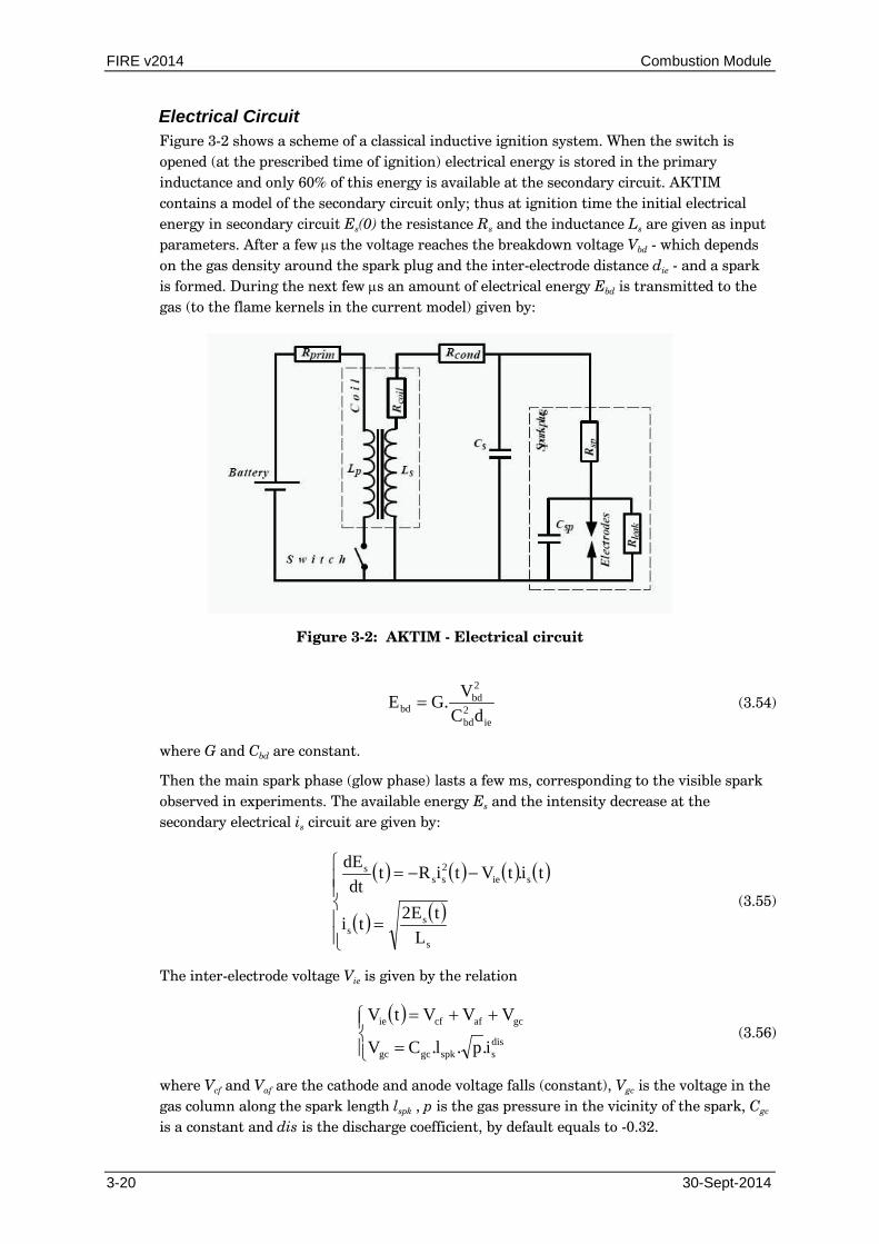
Electrical Circuit Figure 3-2 shows a scheme of a classical inductive ignition system. When the switch is opened (at the prescribed time of ignition) electrical energy is stored in the primary inductance and only 60% of this energy is available at the secondary circuit. AKTIM contains a model of the secondary circuit only; thus at ignition time the initial electrical energy in secondary circuit Es(0) the resistance Rs and the inductance Ls are given as input parameters. After a few µs the voltage reaches the breakdown voltage Vbd - which depends on the gas density around the spark plug and the inter-electrode distance die - and a spark is formed. During the next few µs an amount of electrical energy Ebd is transmitted to the gas (to the flame kernels in the current model) given by:
Figure 3-2: AKTIM - Electrical circuit
ie
2bd
2bd
bd dCV.GE = (3.54)
where G and Cbd are constant.
Then the main spark phase (glow phase) lasts a few ms, corresponding to the visible spark observed in experiments. The available energy Es and the intensity decrease at the secondary electrical is circuit are given by:
( ) ( ) ( ) ( )
( ) ( )
=
−−=
s
ss
sie2ss
s
LtE2ti
ti.tVtiRtdt
dE
(3.55)
The inter-electrode voltage Vie is given by the relation
( )
=
++=dissspkgcgc
gcafcfie
i.p.l.CV
VVVtV (3.56)
where Vcf and Vaf are the cathode and anode voltage falls (constant), Vgc is the voltage in the gas column along the spark length lspk , p is the gas pressure in the vicinity of the spark, Cgc is a constant and dis is the discharge coefficient, by default equals to -0.32.

Combustion Module FIRE v2014
30-Sept-2014 3-21
During the glow phase the inter-electrode voltage Vie may reach the breakdown voltage again. A new breakdown then occurs: the previous spark vanishes and a new one is created. The glow phase lasts as long as electrical energy remains.
Spark Model At the instant of breakdown a spark is initiated between the electrodes. In AKTIM it is represented by a set of Lagrangian particles originally equally spaced between the electrodes. These particles are transported by the mean flow except the ones at the spark extremities (at the cathode and the anode). An arc curvature effect is included, depending on the gas dynamics viscosity (Figure 3-3). The distance between adjacent spark particles is maintained inside a given range so that particles are added or removed permanently.
The spark length lspk appearing in the calculation of the gas column voltage (3.56) is the sum of the distances between adjacent spark particles lmean multiplied by a turbulent folding factor arcΞ . The production of turbulent folding can be split into a mean and turbulent
component:
( )
+=Ξ
Ξ
Ξ=
TTarc
arc
meanarcspk
Aa21
dtd1
l.l (3.57)
In the case of strong convection at the spark plug, the spark length can be many times larger than the inter-electrode distance die, involving a direct increase of the gas column voltage Vgc that can lead to a new breakdown. In this case, the spark particles are suppressed and a new set of particles corresponding to a new spark is initiated.
Figure 3-3: Spark Particles and Flame Kernel Centers at Breakdown Time (left) and Later (right)

FIRE v2014 Combustion Module
3-22 30-Sept-2014
Flame Kernel Model The flame kernel model draws its inspiration from the Discrete Particle Ignition Kernel (DPIK) model of Fan et al [3.24].
At instants of breakdown, a set of around NK=4000 Lagrangian flame kernels are initiated along the spark (Figure 3-3). Each of them represents the gravity center of a possible flame kernel, having a statistical weight 1/NK. Each flame kernel is initially a sphere of imposed radius 0.005mm containing the fresh gas mass mfr that will be burned during the combustion initiation phase:
ie2efffrfr dRm πρ= (3.58)
where Reff = 2mm, and an excess of energy equals to 0.6Ebd provided by the electrical circuit.
The flame kernels are then transported by the mean gas flow and a turbulent dispersion effect similar to the one of O'Rourke (refer to the Spray Manual) for the fuel spray is added.
During the glow phase, the kernels receive the electrical power Qe from the spark:
sgcspk
iee i.V.
ld5.0expQ
−= (3.59)
When the critical energy Ecrit is reached the kernel ignition occurs and a fraction of the fresh gas mass mfr is used to initialize the kernel burnt gas mass i
bm . The critical energy is
given by:
2Lspkcrit 4.p.l
1E πδ
−γγ
= (3.60)
where p is the local gas pressure and δl the local flame thickness. In car engine applications the critical energy is reached instantaneously. After the ignition, the evolution of each
flame kernel i is determined by the evolution of its excess of energy iE and its burnt gas mass i
bm :
−=
ρ=
iWe
i
iLeff
iefffr
ib
QQdt
dE
USdt
dm
(3.61)
where frρ is the fresh gas density as calculated by the ECFM model, ieffS is the effective
kernel surface, iLeffU is its laminar flame speed and i
WQ is the wall heat loss. The flame
kernel combustion is accompanied by a fuel consumption in the gas phase, in cells included into the flame kernel volume.

Combustion Module FIRE v2014
30-Sept-2014 3-23
Figure 3-4: Flame Kernel Real Size at Breakdown Time (left) and Later (right)
The effective kernel surface is given by:
( )
πρ
=
πΞ=3/1
ib
ibi
2iiW
ieff
4m3r
r4..fS (3.62)
with ir the kernel radius - increasing with time as proportional to the burnt mass fraction
(Figure 3-4) - ibρ the burnt gas density inside the kernel (see eq. 3.75), iΞ the turbulent
folding of the surface and wf a wall factor. The turbulent folding factor iΞ models the
stretching and quenching of the kernel surface. Its evolution is treated by the ITNFS model [3.39]. The wall factor wf measures the part of the kernel surface which is in contact with
the spark plug walls and therefore is inactive as far as the kernel combustion is concerned. If there is no overlapping, the factor is equal to 1.
The effective laminar flame speed iLeffU in relation (3.61) is given by:
( )
δ=ζ
−+ζ+−ζ+ζ−=
iLi
bibi2ii
LiLeff
r2
400TT1211.U.5.0U
(3.63)
where ibT is the burnt gas inside the ith kernel. The kernel burnt gas temperature and
density are related by:
ρ=ρ
+=
ib
bb
ib
bi
.b
i
bib
TT
CpmETT
(3.64)
Finally, the wall heat loss term iWQ in equation (3.61) is calculated as:
( )SPib
iW
iW TT.S.hQ −= (3.65)

FIRE v2014 Combustion Module
3-24 30-Sept-2014
where h is a given heat transfer coefficient equal to 2000 W/m2K, iWS is the contact surface
between the flame kernel and the spark plug and SPT is the spark plug temperature. When
using AKTIM, it is recommended to mesh the spark plug in order to correctly capture the flow dynamics and wall heat transfer. In particular the kernel-wall contact surface and the spark plug temperature are then accurately computed. However if the spark plug is not meshed, the wall heat loss relation (3.65) still applies using Tspk = 600K and a rough evaluation of the contact surface based on the distance between the flame kernel center and the cathode/anode locations.
When the combustion of a flame kernel ends, its surface is deposited as flame surface density randomly in a cell contained into the kernel volume, thus initializing the ECFM model.
ISSIM - Imposed Stretch Spark Ignition Model This new Eulerian multi-spark ignition model (ISSIM) is based on the electrical circuit model of AKTIM as described in the previous chapter which provides the spark length and duration and estimate the energy transferred to the gas and the amount of burnt gas mass deposited at the spark. At ignition timing an initial burned gas profile is created. Then, the reaction rate is directly controlled by the flame surface density (FSD) equation whose source terms are modified to correctly represent flame surface growth during ignition. As long as a spark exists, a spark source term is added to the ECFM in order to ensure the flame holder effect at the spark. The usage of the FSD equation naturally allows multi-spark description (i.e. modeling more than one spark plug at a time or multiple firings of a single spark, or combinations of both).
The ISSIM model can only be applied with the ECFM-3Z combustion model and not with the ECFM.
The ISSIM model has a much simpler structure than the former Lagrangian AKTIM model and presents some clear advantages that should improve the simulation of SI engines:
• Both the early ignition and turbulent propagation phases are consistently modeled since the flame surface density equation is transported from the very beginning of spark ignition;
• The model provides the amount of burnt gas mass deposited in the vicinity of the spark, the spark source term in the ECFM equation and the corresponding fuel consumption rate;
• During ignition, the flame growth is not controlled by a 0D model, but directly by the ECFM equation using local evaluations of the Eulerian fields. This has two advantages:
1. It appropriately accounts for the effect of mixture stratification in the vicinity of the spark which is not the case with AKTIM;
2. It accounts for the aerodynamic effects resulting from the mean flow and turbulence at the spark and the resulting spark and flame stretch;
• It accounts for the flame holder effect and provides means to integrate a blow-off in the case of excessive convection at the spark;
Combustion Module FIRE v2014
30-Sept-2014 3-25
Electrical Circuit The electrical system model is described in the previous chapter and is based on the electrical circuit model of the Lagrangian AKTIM (classical inductive ignition system) using the same formulas and equations.
Spark Model At breakdown the spark length is equal to the spark gap ied . Then, the spark is stretched
( meanl ) by mean convection and turbulent motion of the flow. The total length of the spark
is spkl as given in the same equation (3.57) as for AKTIM. The model for the spark
wrinkling by the turbulent flow arcΞ is given by the spark wrinkling evolution equation
which has the same form as for AKTIM (see equation (3.57)) where Ta and TA are the
spark strain by the turbulent and the mean flow, respectively. Ta corresponds to the effect
of the turbulent eddies greater than the arc thickness cl and lower than the half length of
the spark Ml . cl is estimated as follows:
s
sc D
ilπ
2= (3.66)
where SD is the current density at the electrode surface, which is of the order of 100 A/cm2
during glow mode. Ml is simply written:
spkM ll21
= (3.67)
The computation of the strain Ta is similar to the ITNFS function in the equation of the
flame surface density equation:
t
T lua
′Γ= (3.68)
where tl is the integral length scale of turbulence and u′ is the corresponding fluctuation
velocity.
( ) ( )2
32
3
,max,max23
)2ln(28.0
−
=Γ
tM
t
c
t
lll
ll
η (3.69)
The mean strain TA is the contribution of the mean flow and it is expressed as follows:
M
T luA
′= (3.70)
The mean spark length meanl can be affected by the flow convection assuming a rectangular
shape for the spark, so that the equation for meanl reads:
( )txudt
dlspk
mean ,~2= (3.71)
FIRE v2014 Combustion Module
3-26 30-Sept-2014
where ( )txu spk ,~ is the resolved velocity field at the spark plug.
Spark and Flame Kernel Coupling During the arc and glow phases, only a fraction of the spark energy is released to the gas. The energy released in a thin region near the electrodes is essentially lost by fall voltage. The energy loss to the electrodes during the glow phase is about 70-80%. The potential difference between both electrodes, also called spark voltage is written:
gcafcfspk VVVV ++= (3.72)
where cfV is the cathode fall voltage, afV is the anode fall voltage and gcV is the gas
column voltage. The anode fall voltage is similar for the arc and glow modes and equal to 18.75 V for Inconel (an alloy based on Nickel, Chrome and iron). The cathode fall voltage is 7.6 V during arc phase and 252 V during glow phase for Inconel. The gas column voltage is approximately equivalent:
aniegc piCdV −= (3.73)
where C is a constant (6.31 during arc phase and 40.46 during glow phase), i is the circuit intensity through the gas column (in A), n is a constant (0.75 during arc phase and 0.32 during glow phase), ied is the spark gap, p the pressure, a is a constant equal to 0.51.
The voltage on the gas column depends on the spark length. The expression (3.73) is available only for non-convective and non-turbulent flows.
The description of the breakdown and arc phases is very complex: extremely short duration, presence of a plasma channel, very high temperatures and unsteady behavior. The modeling of these modes is therefore a complex issue which is not computed but the initial conditions are set for the spark discharge in terms of energy deposition. The energy deposited after these phases is expressed as a function of the spark gap and of the breakdown voltage:
2
=
KV
dCE bd
ie
bdbd (3.74)
where mJCbd 125.0= . K is also a constant (for air mm
kVK 5.1= ).
The energy transferred to the gas is:
( ) bdignign EtE 6,0=∆ (3.75)
The breakdown voltage is written:
iecbd dKFV
=
0
21
ρρ
(3.76)
where 0ρ is the density at standard conditions (300K, 1bar) and cF is a correction
function. At the first breakdown:

Combustion Module FIRE v2014
30-Sept-2014 3-27
=
0
0
,1.0max
,16max
ρρ
ρρ
cF (3.77)
In the case of restrike (by convection), 1=cF .
In practice bdV can be affected by unsteady effects. Moreover, it does not include the effect
of the electrode geometry and material. It may be noticed that contrary to the gas column voltage, the breakdown voltage is controlled by the gas density (and not the pressure) near the electrode surface.
Before the spark is created, the voltage between the electrodes spkV increases with the rise
rate of 1 kV/ms. When the breakdown voltage is reached a spark is formed and an amount of energy (Eq. (3.75)) is deposited to the gas. After that, the energy provided to the gas during the glow phase is computed. During the glow phase, the voltage fall is localized in the vicinity of the electrodes. Therefore it is assumed that the energy released within these regions is lost to the electrodes. Finally, the energy transferred to the gas is deduced from the gas column voltage and the intensity as follows:
( ) ( ) ( )titV
dttdE
sgcign = (3.78)
where the gas column voltage is written:
51.032.046.40 pilV sspkgc−= (3.79)
To incorporate the effect of the electrode diameter (del) on the spark efficiency, a correction function is added to the gas column voltage resulting in the following formula:
spk
el
ld
sspkgc epilV 251.032.046.40 −= (3.80)
This energy ignE is used to determine if ignition is successful or not. The critical ignition
energy is retained:
241 Lspkc plE δπ
γγ−
= (3.81)
While ( ) ( )tEtE cign < , the flame kernel is not created. On the contrary, if ( ) ( )tEtE cign > , a
flame kernel is formed around the spark and ignition starts. In that case, an amount of burnt gas mass is deposited at the spark which corresponds to a cylinder with radius Lδ2
and height spkl :
lg
24spkpLspku
ignb lm πδρ= (3.82)

FIRE v2014 Combustion Module
3-28 30-Sept-2014
ISSIM-LES (Large Eddy Simulation) Spark Ignition Model ISSIM-LES describes the early flame kernel development in a way that is required by the LES framework allowing the following ignition features like:
• multi-ignition in time and space,
• re-ignition and
• “flame holder” effect under strong convection condition around the flame kernel.
The ISSIM-LES approach used in FIRE is based on the description given by Colin and Truffin [3.16], where the modified transport equation for the flame surface density (FSD) (see chapter 3.2.4.3.7. for more information) can be expressed as:
( ) ( ) ( ) ignl
bP
dsgsressgsressgsres Sr
NSCCSSTTt Σ+ΣΞ+−+Σ⋅∇−+++++=
∂Σ∂ ωτααααα
121
where α remains close to zero during ignition and equal unity when ignition is over. Therefore ( )
P
dresres NSCS Σ⋅∇−+ is suppressed during ignition and replaced by the term
( ) ΣΞ+ lb
Sr
τ12
. In the above equations Ξ represents the turbulent wrinkling factor, br the
flame kernel radius and ignΣω is the FSD ignition source term. These terms can be defined
as:
( ) ( )( )Nccwithc
Nccc c
c ~~
−⋅∇+Σ=Σ∇
−⋅∇−Σ=
∇Σ
=Ξ
31
4330,max
==Σ
Σ−Σ= ∫Σ dVcrand
rcwith
dt ignbb
igncignign
πω
ignc represents a Gaussian profile of the initial volume fraction and is defined as (c0 is a
constant and xspark is the spark plug position):
2
ˆ6.00
∆
−−
=
sparkxx
ign ecc
Note: The ISSIM-LES approach can only be used with the ECFM-3Z combustion model in combination of activated laminar terms and one of the 2 turbulence models, LES or LES-CSM, respectively.
Combustion Module FIRE v2014
30-Sept-2014 3-29
3.2.4.3.6. Laminar Terms for the Flame Surface Density Equation The additional source term for the flame surface density equation, which considers the contribution of laminar reactions consists of three terms:
P considers the propagation of the flame:
Σ⋅−∇= NSP L
frρρ
(3.83)
C considers the creation and destruction of flame surface by the curvature:
( )Σ⋅∇= NSC Lfrρ
ρ (3.84)
S considers the straining of the flame by all structures of turbulence:
( )Σ∇−⋅∇= uNNuS ~:~ (3.85)
with: ccN
∇∇
−=
3.2.4.3.7. Large Eddy Simulation (LES) Terms for the ECFM / ECFM-3Z combustion model
The following chapter describes the modifications, which are necessary for the FSD transport equation and source terms in the framework of LES.
The CFMLES method was first introduced by Richard et al. in 2007 [3.53] where modifications of the diffusion and source terms were introduced in order to keep the flame
brush thickness equal to filtxn∆=∆ with filtn as model parameter (5 to 10). Scale ∆
represents a combustion filter size which is filtn times larger than the LES grid scale x∆ .
Therefore instantaneous quantities can have now 3 different mathematical formalisms as given in the following:
scalelength filtered thickened...ˆ valuefiltered Favre...~
valueaverage cell...
φφφ
The introduction of the combustion filter size is done since eddies smaller than the flame thickness are not able to wrinkle the flame front [3.15]. The flame brush thickness
cnδ should be equal to the combustion filter size ∆ which is controlled by the controlling
factor F. The controlling factor should ensure the equality [3.53]:
∆=∆= ˆxrescn nFδ (3.86)
The derivation of the controlling parameter is based on the natural flame brush thickness, grid spatial resolution and corresponding equilibrium wrinkling factor used as an estimator for SGS (sub-grid scale) turbulence level inside the cell.
FIRE v2014 Combustion Module
3-30 30-Sept-2014
The FSD equation, as a part of the CFMLES combustion approach, is derived according to [3.53] filtered to the combustion filter and split into resolved and unresolved parts:
PCCSSTTt sgsressgsressgsres ++++++=
∂Σ∂
(3.87)
where Tres, Sres, Cres and P are the transport, strain, curvature and propagation terms due to resolved flow motions (see chapter 3.2.4.3.6) and Tsgs, Ssgs and Csgs are the unresolved transport, strain and curvature terms, respectively, with:
( ) ( )
( ) ( ) ( )
P
d
C
lamL
C
d
S
llcST
t
tc
T
NSccccSNS
uSuuNNu
Scu
t
sgs
res
sgs
res
sgs
res
Σ⋅∇−ΣΣ−Σ−−
+Σ⋅∇
+Σ∆
′
∆′Γ+Σ∇−∇+
Σ∇⋅∇+Σ⋅∇−=
∂Σ∂
)1(
ˆˆˆ
,ˆ~:~ˆ~~
*
0,*β
δσυ
σ
(3.88)
Displacement speed is calculated from the conservation of mass through the flame front:
ρρ
ρρ frldfrld
SSSS =→= (3.89)
and the normal to the flame front N is calculated as above (see chapter 3.2.4.3.6.) as normalized gradient of the reaction progress variable field. The Gamma function in the above FSD equation is derived in [1001] and adopted for the CFMLES in [999]. It represents the effective strain of the flame by turbulence at all relevant scales smaller than
∆ .
The fluctuation velocity is obtained from dimensional relations and simple Smagorinsky-like model (Cs= 0.12):
~
'ˆXs
t
Cu
∆=
ρµ
(3.90)
Lδ is the flame thickness from Bint’s correlation described above. Inputs for Csgs are
laminar FSD and Bray-Moss-Libby expression [999] as:
( ) ( )1~~~ +=⋅∇−+∇=Σ τρρ
fr
lam ccandNccc (3.91)
Finally the controlling parameter F can be defined as:
Combustion Module FIRE v2014
30-Sept-2014 3-31
)1(
ˆˆˆ
,ˆˆ
8
ˆˆˆ
,ˆ
21 K
uSu
ScScK
uSun
F
llct
tcc
llcxres
−
∆
′
∆′Γ
+
∆
′
∆′Γ∆
=
ρ
δσυσυσ
δσ (3.92)
Model parameters K1 and K2 are obtained from the thermal expansion rate 1−= bfr ρρτ as:
( )
++−
++
+=
21
3211
1
2*
*
1ττττ
τβ cK (3.93)
τ
β+
−=1
1**
2cK (3.94)
with 5=resn , 34* =β and 5.0* =c .
cσ is a correction factor in the expressions of the diffusivity and SGS strain and can be
expressed as:
( ) ( )
∆
′
∆′Γ
++−
++
+−Ξ
=∆
=
ˆˆˆ
,ˆ
31
3211
114
2*
*
uSu
cSwith
n
ll
eql
cncn
xresc
δ
τττττ
β
δδ
σ (3.95)
and eqΞ is the equilibrium wrinkling factor given by:
∆′=
+−
∆
′
∆′Γ
+=Ξ ˆˆˆ
11
ˆˆˆ
,ˆˆ
21 * uCandc
uSu
S stll
t
leq υ
τβ
δυ
(3.96)
Note: The LES approach using the unresolved source terms for the FSD can only be used with the ECFM and ECFM-3Z combustion model in combination with activated laminar terms and one of the 2 turbulence models, LES or LES-CSM, respectively.

FIRE v2014 Combustion Module
3-32 30-Sept-2014
3.2.4.4. ECFM-3Z Model The existing ECFM model is devoted to gasoline combustion. The ECFM-3Z model was developed by the GSM consortium (Groupement Scientifque Moteurs) specifically for Diesel combustion. This is a combustion model based on a flame surface density transport equation and a mixing model that can describe inhomogeneous turbulent premixed and diffusion combustion. The model relies on the ECFM combustion model, previously described and implemented in FIRE and on a three areas mixing description. Further it is coupled with an improved burnt gas chemistry description compared to ECFM.
Up to now the ECFM-3Z combustion model was only applicable for auto-ignition cases, although the code is prepared to handle for both ignition procedures, auto-ignition and spark ignition,. Now the gasoline engine ECFM combustion model can also be activated via the ECFM-3Z mode using all the attractive features such as the general species treatment or separate CO/CO2 oxidation reaction mechanism. So all standard engine applications can be done now with only one identical combustion model.
Figure 3-5: Zones in ECFM-3Z Model
3.2.4.4.1. Multi-Component Capabilities for the ECFM-3Z Model When using the ECFM-3Z model it is possible to define the fuel as consisting of more than one chemical species. The fuel can be prescribed as a mixture of several components. In principal an arbitrary number of fuel components is possible, but it is recommended to use a mixture of up to 6 or 8 hydrocarbons. By using this number of components each group of hydrocarbons can be represented. This description is available for all types of combustion.
The provided solution enables a connection to the multi-component spray capabilities. If in the spray module the fuel is defined as consisting of several components, then the same components can be chosen in the gas phase set-up (refer to the Species Transport Manual). Since the Lagrangian and the gas phase have to be connected, it is important to prescribe the same index for each fuel component in the spray module and the gas phase initial conditions set-up.
Combustion Module FIRE v2014
30-Sept-2014 3-33
The ECFM-3Z combustion model uses the fuel components to combine them temporarily to a fuel mixture during the calculation. This means that effects like auto-ignition and flame propagation are handled for this combined fuel within the combustion model. The rate of reaction for each fuel component is finally split up. By doing this it is possible to calculate the consumption of each component separately. The development of the combustion products is based on the consumption of the single components.
3.2.4.4.2. The Global Species Equations Compared to the standard ECFM model, the ECFM-3Z model takes into account:
• three new tracers for NO, CO and H2 in order to know the mass fractions in the unburned gases,
• two species describing the mixing, FFuρ and A
O2ρ (only used to rebuild mixing
quantities)
• and an intermediate species for auto-ignition Iy~ .
Thus six more scalars are taken into account.
In the ECFM-3Z model, the transport equations are solved for the averaged quantities of chemical species O2, N2, CO2, CO, H2, H2O, O, H, N, OH and NO. Here, averaged means these quantities are the global quantities for the three mixing zones (that is in the whole cell). Therefore, the term "burnt gases" includes the real burnt gases in the mixed zone
(zone bM in Figure 3-5) plus a part of the unmixed fuel (zone bF in Figure 3-5) and air
(zone bA in Figure 3-5). This equation is classically modeled as:
Xi
X
t
t
ii
XiX
xy~
ScScxxy~u~
ty~
ω=
∂∂
µ+
µ∂∂
−∂
ρ∂+
∂ρ∂
(3.97)
where Xω is the combustion source term and Xy~ is the averaged mass fraction of species
α.
The fuel is divided in two parts: the fuel present in the fresh gases, uFuy~ and the fuel
present in the burnt gases, bFuy~
ρρ
===ρ
ρ===
bFu
bFu
bFub
Fu
uFu
uFu
uFuu
Fu V/mV/m
mmy~and
V/mV/m
mmy~ (3.98)
with bFu
uFuFu y~y~y~ += as the mean fuel mass fraction in the computational cell. u
Fum (resp. bFum ) is the mass of the fuel contained in fresh gases (resp. burnt gases). A transport
equation is used to compute uFuy~ :
uFu
uFu
i
uFu
t
t
ii
uFui
uFu S
~xy~
ScScxxy~u~
ty~
ω+ρ=
∂∂
µ+
µ∂∂
−∂
ρ∂+
∂ρ∂
(3.99)
where uFuS is the source term quantifying the fuel evaporation in fresh gases. u
Fuω is a
source term taking auto-ignition, premixed flame and mixing between mixed unburned and mixed burnt areas into account.
FIRE v2014 Combustion Module
3-34 30-Sept-2014
3.2.4.4.3. The Mixing Model The amount of mixing is computed with a characteristic time scale based on the k-ε model. During evaporation, it is necessary to specify the amount of fuel going into the mixed zone (from zone F to M=Mu+Mb) and the amount going into the "pure fuel" zone (into zone F=Fu+Fb).
For a diesel spray, the fuel droplets are very close to each other and are located in a region essentially made of fuel. After the evaporation of the fuel, an adequate time is needed for the mixing from the nearly pure fuel region with the ambient air (mixing from zone F and A to M).
In this case, the mixing of fuel with air is modeled by initially placing the fuel into the ‘pure fuel’ zone. So, the fuel which evaporates from a droplet is released in the pure fuel zone F=Fu+Fb).
In order to describe the three mixing zones, two new quantities are introduced: the
unmixed fuel FFuy~ ( F,b
FuF,u
FuFFu y~y~y~ += ) and the unmixed oxygen A
O2y~ ( A,b
OA,u
OAO 222
y~y~y~ += ).
The equations for these unmixed species are:
MA
Oi
AO
ii
AOi
AO
MFFu
FFu
i
FFu
ii
FFui
FFu
2
222 Exy~
Scxxy~u~
ty~
ES~
xy~
Scxxy~u~
ty~
→
→
ρ=
∂
∂µ∂∂
−∂
ρ∂+
∂
ρ∂
ρ+ρ=
∂∂µ
∂∂
−∂
ρ∂+
∂ρ∂
(3.100)
The mixing model is described by the source terms MFFuE → and MA
O2E → in the unmixed fuel
and unmixed oxygen equations. The amount of mixing is computed with a characteristic time scale based on the k-epsilon model:
ρρ
−τ
−=
ρρ
−τ
−=
+∞
→
→
EGRairu
u
M
O
AOA
Om
MAO
Fuu
u
MFFu
FFu
m
MFFu
MM
y~y~
1y~1E
MMy~1y~1E
2
2
22
(3.101)
In equation (3.101), MM is the mean molar mass of the gases in the mixed area, FuM is
the molar mass of fuel, 2OM is the molar mass of O2, EGRairM + is the mean molar mass of
the unmixed air+EGR gases, ρ is mean density, u
uρ is the density of the unburned gases
(the density of fresh gases that would be obtained if combustion had not occurred), ∞2Oy~ is
the oxygen mass fraction defined by equation (3.103) and mτ is the mixing time defined as:
km
1m
εβ=τ− (3.102)
mβ is a constant with the default value 1. The oxygen mass fraction in the unmixed air is
computed as follows:

Combustion Module FIRE v2014
30-Sept-2014 3-35
TFu
TOO y~1
y~y~ 2
2 −=∞ (3.103)
where 2TOy~ and TFuy~ are the oxygen and fuel tracer respectively.
3.2.4.4.4. Conditional Compositions
Mixed Zone In order to reconstruct the mixed and unmixed parts, as mentioned above, two species have
been introduced, unmixed fuel and unmixed oxygen ( FFuy~ and A
O2y~ ). Knowing these two
quantities, the mixed quantities can be constructed.
The main assumption is that the unburned gas composition of air+EGR is the same in the mixed and unmixed areas. Thus if the total amount of oxygen (the oxygen in the mean/total
cell) and the unmixed oxygen ( AO2
y~ ) is known, then the mass ratio of air + EGR mixed over
total air + EGR (in the total cell) is known.
The mass of fuel tracer in the mixed area is obtained directly from the difference between the fuel tracer and the unmixed fuel, as for the oxygen species:
AOTO
MTO
FFuTFu
MTFu
222ρ−ρ=ρ
ρ−ρ=ρ (3.104)
For the unburned and burnt fuel mass fractions the unmixed part must be subtracted from the unmixed fuel zone:
( )
FFu
bFu
M,bFu
FFu
uFu
M,uFu
c~c~1
ρ−ρ=ρ
ρ−−ρ=ρ (3.105)
with the Favre averaged progress variable:
TFu
uFu
u
y~y~1
mm1c~ −=−= (3.106)
For the other species α we define a coefficient AO2
c which is the ratio of the unmixed O2 to
the oxygen tracer.
TX
AX
TO
AOA
O y~y~
y~y~
c2
2
2== (3.107)
where TXy~ is the mass fraction of the tracer of the X species: for species O2, CO, NO, Soot
and H2, a transport equation is directly solved for these tracers as shown in the previous section. For species N2, CO2 and H2O, the tracers are reconstructed from the N, C and H atom balance equations.
FIRE v2014 Combustion Module
3-36 30-Sept-2014
Fresh and Burnt Gases There are two ways to obtain the burnt gas properties depending on the value of the progress variable c. When the value of c exceeds 0.05, these properties are deduced from the mean and the unburned gas quantities using the classical relationship between the mean value, the unburned one, the burnt one and c. When the value of c is too low, we obtain these quantities assuming they are the result of a complete combustion (+ equilibrium) under the local thermo-chemical conditions.
Previously it was described how to define the equivalent quantities in the mixed zone, starting from the mean species mass fractions and enthalpies. Now, the mixed zone itself will be divided into fresh and burnt gas zones.
In all CFM models, the flame front is described as an infinitely thin interface that separates fresh and burnt gases. In order to correctly compute the laminar flame speed in the fresh mixture and the pollutant formation in the burnt gases, the species mass fractions must be
known precisely in these two regions, M,u
M,uXy~ and
M,b
M,bXy~ (These quantities are
evaluated if: c>0.05, and if the mass fraction occupied by the mixed zone is 95.0FA
<ρ
ρ +
.
These mass fractions are defined as:
M,u
M,uX
M,u
M,uX m
my~ = (3.108)
M,b
M,bX
M,b
M,bX m
my~ = (3.109)
where M,um (resp. M,bm ) is the unburned (resp. burnt) mass in the mixed zone defined by:
( )
MM,b
MM,u
mc~mmc~1m
=
−= (3.110)
where Mm is the total mass in the mixed zone of the cell.
3.2.4.4.5. The Auto-ignition Model The ignition delay is computed either through a correlation or through an interpolation from tabulated values. An intermediate species integrates the advance in the auto-ignition process. When the delay time is reached, the mixed fuel is oxidized with a chemical characteristic time.
The Auto-ignition Delay The auto-ignition of the unburned mixture is computed over the unburned mixed gases. The ignition delay is obtained by different means, depending on the parameter specified by the user in the GUI:
The correlation used for diesel combustion is:
( ) ( ) ( ) u
2
T5914
13.0u05.0
M,u
M,uFu
53.0
M,u
M,uO
8d eNN10804.4 ρ×=τ
−− (3.111)

Combustion Module FIRE v2014
30-Sept-2014 3-37
where molar concentrations are given in mole per cubic meter, the temperature in K, the
density uρ in kg/m3.
The tabulation of n-heptane auto-ignition delay is done over a specific range of pressures, temperatures, equivalence ratio and EGR rates. Two versions of accessing the tabulated values are available. The first one is calculating the ignition delay time according to a one-step ignition behavior. The second approach is treating the ignition delay as a two-step event which includes also the cool flame burning under lean and low temperature conditions.
The Intermediate Species The intermediate species Iρ has the same evolution equation as the fuel tracer TFuρ
without the source term due to spray evaporation. Assuming the mass of intermediate species in zones F and A is zero and that its molar mass is equal to the fuel molar mass, therefore the conditioned molar concentration reads:
Fu
VI
M
MI M
CN Mρ
= (3.112)
The intermediate species increases in time with the following source term:
( )dM
MTFu
M
MI FNt
Nτ=
∂
∂ (3.113)
where F is a function of the delay time dτ :
( )( )
d
21
M
MTFu
M
MI
d2d
2
d
N
NB14B
Fτ
τ−+τ
=τ (3.114)
where B is a constant set to 1s. The F function was chosen to avoid time step dependency for auto-ignition.
Oxidation of the Fuel The auto-ignition delay is reached when the molar concentration of intermediate exceeds
the molar concentration of the fuel tracer M
MTFuM
MI NN > . The mixed fuel is oxidized with
a chemical characteristic time. The fuel molar concentration evolution is:
c
M
M,uFuM
M,uFu N
t
N
τ−=
∂
∂ (3.115)
The chemical characteristic time cτ is defined by:
ba
TT
0cc eτ=τ (3.116)
where aT is an activation temperature set to 6000 K, and the constant 0cτ is equal to 5 x 10⁻⁵s.
FIRE v2014 Combustion Module
3-38 30-Sept-2014
3.2.4.4.6. Oxidation Kinetics of the Fuel The premixed flame and the auto-ignition in the fresh gases lead to a sink term of fuel in the unburned mixed zone. This fuel is then oxidized by the model presented in this section. This oxidation leads to the formation of CO and CO2 in the burned gases.
For the ECFM-3Z, a different fuel conversion mechanism (2-step chemistry mechanism) is used compared to the ECFM. Due to the introduction of CO/CO2 kinetics the fuel oxidation model has been modified. The same model is used for auto-ignition and premixed flame consumption.
In the Unburnt Gases As previously mentioned, the model is enriched by new unburned gases species. It is assumed that the unburned gas composition includes fuel, O2, N2, CO2, CO, H2O, H2, NO. Thus compared to the standard ECFM model, three more tracers need to be introduced, CO tracer, H2 tracer and NO tracer. These tracers should be introduced in the balance equations when the conditioned burnt gas concentrations are computed. The oxidation of the fuel is decomposed in two phases:
• A first partial oxidation of fuel is realized which leads to the formation of a great amount of CO, and a few CO2, in the burnt gases of the mixed zone.
• In the burnt gases of the mixed zone, the CO previously generated is oxidized to CO2.
This new oxidation mechanism provides a more accurate description of the formation of CO in the case of lean mixtures.
Assuming the mean fuel composition is zyx OHC , where coefficients m, n and l were
previously defined for a mono or multi-component fuel, a function of the local mean
equivalence ratio φ is then defined as:
0ifyx2
x22z
4yx98.04
if
1if
2
21
1
=α→φ<φ
+
−φ
−+×
=α→φ<φ<φ
=α→φ<φ
(3.117)
where 99.01 =φ and crit2 9.0 φ=φ , with critφ the critical equivalence ratio above which
there is not enough oxygen to complete the oxidation of fuel into CO:
−+=φ
2z
4yx
x2
crit (3.118)
If φ<φ2 , a part of the unburned fuel M
M,uFuy~ cannot be oxidized and is transferred instead
into the burnt gases as a source of burnt gas fuel M
M,bFuy~ in the mixed zone. The source of
burnt gas fuel is given by:

Combustion Module FIRE v2014
30-Sept-2014 3-39
φ
φ−−=→ critu
Fubu
Fu 9.01dNdN (3.119)
We have [ ] [ ]φ
φcrituECFMAIlmn
uefflmn OHCdOHCd ⋅⋅= +9.0 when 2φ>φ with [ ]u
efflmn OHCd
as the effective sink term for unburned fuel and [ ]uECFMAIlmn OHCd + as the sink term due
to auto-ignition and premixed flame.
For O2, CO2, H2O, CO and H2 the source terms are:
( )( )
( )
( )[ ]
( )2y1dNdN
xr11dNdN2ydNdN
xr1dNdN4yr11
2xdNdN
uFu
uH
COuFu
uCO
uFu
uOH
COuFu
uCO
COuFu
uO
2
2
2
2
α−−=
−α−−=
α−=
−α−=
α+−α+=
(3.120)
In the Burnt Gases Due to very rich premixed flames or the diffusion of unmixed fuel in the burnt mixed region, it is possible to find fuel in the burnt gases. It is assumed that the combustion is controlled by chemistry in the mixed zone, the mixing process being described by the mixing between zones. Therefore, the model already used for the oxidation by auto-ignition is the first simple model to be adopted.
c
M
M,bFuM
M,bFu N
t
N
τ−=
∂
∂ (3.121)
where cτ is given by equation (3.116).
3.2.4.4.7. The Regression Model In order to compute multi-injection or local extinction, a simplified regression model has been introduced. This model transfers burnt gas quantities into unburned gas quantities when the local burnt gas temperature is too low.
First the coefficient FFuTFu
II y~y~
y~c~−
= is defined, which defines the state of the auto-ignition
process. The regression model is used if auto-ignition is switched on:
if 1c~I < , the auto-ignition delay has not been reached yet, there is no
combustion by auto-ignition in the fresh gases.
if 1c~I = , the auto-ignition delay has been reached, the combustion by auto-
ignition in the fresh gases is under way.
FIRE v2014 Combustion Module
3-40 30-Sept-2014
In every cell where 999.0c~I > (local condition and local modification of variables), it is
considered that the auto-ignition combustion process is finished, the auto-ignition delay calculation can be restarted by imposing 0c~I = , that is: 0y~I = .
A temperature deavT is defined, which represents the minimum temperature allowed in the
burnt gases. If the burnt gas temperature bT is lower than K200Tdeav + (with
K1200TT cutdeav == in practice), it is considered that the reactions in burnt gases are
progressively stopped. In this case the burnt gases have to be transferred to the unburned zone.
3.2.4.4.8. Post Flame Chemistry As the conditional quantities are known, it is possible to compute chemistry in a conditional way. Thus all the auto-ignition chemistry is computed using the unburned gas properties and all the pollutant, post oxidation and equilibrium chemistry is computed using the burnt gas properties. Thus the mean gas properties are updated through burnt gas properties modification.
In the ECFM-3Z model, the approach is the same as for ECFM model. Knowing the burnt gases composition and burnt gas temperature, the procedure starts with calculating the post flame chemistry. This operation is an iterative process, which modifies the burnt gases composition and the burnt gas temperature.
The new burnt gas composition is used to update the mean mass fractions and the new burnt gas temperature is used to update the mean enthalpy.
After the calculation of M,b
M,bXy~ by the burnt gas combustion model, an equilibrium
computation and a pollutant formation are performed to correct the burnt gas state and temperature.
The post-flame chemistry of the model is an improved version of the ECFM model. The major change is the introduction of a kinetic oxidation of the CO. Thus, the CO/CO2 equilibrium is no longer considered in the equilibrium package. An equilibrium resolution of the remaining set of equations was rewritten.
The considered equilibrium reactions are:
222
22
2
2
2
H2OOH2HOOH2
H2HO2ON2N
+↔+↔
↔↔↔
(3.122)
The N2/N reaction can be treated separately as in the ECFM. The other set of equations can be reduced in one polynomial equation (6th degree). This equation is then solved using a Newton method, which is straightforward with a polynomial expression. The considered kinetic oxidation of CO is:

Combustion Module FIRE v2014
30-Sept-2014 3-41
HCOOHCO 2 +↔+ (3.123)
This system is solved based on the burnt gas composition and temperature, which allows
the estimation of the species mass fractions M,b
M,bXy~ given by the turbulent combustion
model to be corrected. Finally, these new estimates of M,b
M,bXy~ are considered in the
averaged mass fractions Xy~ .
3.2.5. Probability Density Function Approach The PDF combustion model, available in FIRE, takes into account the simultaneous effects of both finite rate chemistry and turbulence, and thus obviates the need for any prior assumptions as to whether one of the two processes is limiting the mean rate of reaction. Additionally, benefits of the PDF approach lie in the fact that it provides a complete statistical description of the scalar quantities under consideration. Thus, it allows first (mean values), second (variance), and even higher (skewness) order moments to be easily extracted, and that the term expressing the rate of chemical reaction appears in closed form; i.e. requires no modeling.
In this method, the thermochemistry of the reactive mixture is expressed in terms of a reaction progress variable c (which is algebraically related to yfu), the mixture fraction f, and the enthalpy in order to account for non-adiabatic bulk compression effects on temperature.
The reaction progress variable c is defined as:
∞
=Pr,
Pr
yyc (3.124)
where ∞Pr,y is the maximum product mass fraction to occur, such that either all the fuel
or all the oxidant is depleted (or both for stoichiometric mixtures). The variable c is bounded by the values of zero and unity, corresponding to fully unburned and burnt states, regardless of equivalence ratio.
The current method solves a transport equation for the joint probability density function ( )ψp of the mixture fraction f, the reaction progress variable c, and the enthalpy h by
means of a Monte Carlo Simulation technique. This enables accurate determination of the chemical sources in terms of the instantaneous thermochemical quantities of the reactive system.
3.2.5.1. PDF Transport Equation The single-point PDF equation for the Favre averaged joint probability ( )ψp~ can be
written ([3.51]; [3.52]) as:
FIRE v2014 Combustion Module
3-42 30-Sept-2014
( ) ( ) ( ) ( )
( ) ( )
VIV
p~xJ
p~u x
IIIIII
p~x
pU~t
p~
N
1 i
,i"k
k
N
1kk
∑
ΨΨ=φ∂∂
Ψ∂∂
+ΨΨ=φρ∂∂
−
=∑ ΨΨωΨ∂∂
ρ+∂
Ψ∂ρ+
∂Ψ∂
ρ
=α
α
α
=αα
α
(3.125)
with ( )ψp~ being the probability that at location x and time t, a quantity φ is within the
range ψ+ψ<φ<ψ d .
The quantity ψ is related to the mean density ρ via the following expression:
( )( )
11
0
dp~−
ΨΨρΨ
=ρ ∫ (3.126)
The terms II and IV in equation (3.125) describe the transport of probability in physical space. Turbulent convection is modeled using a gradient-diffusion approximation [3.51].
( ) ( )
∂
Ψ∂σµ
∂∂
=ΨΨ=φρ∂
∂−
kt
t
k
"k
k xp~
xp~u
x (3.127)
Term III of equation (3.125) that expresses the effect of chemical reaction on the probability density function ( )ψp~ appears in closed form and is modeled here as [3.10]
( ) ( )( )
( ) ( )( ) ( )
[ ] [ ]
−⋅=ω
∞ρ
ω=
∞=
RTEexpO HCA
,xYt,xt,x
dtt,xdc
,xYt,xY
t,xc
ay 2
xmnp
p
p
p
p
(3.128)
Term V of equation (3.125) represents turbulent mixing between reactants, products, and intermediate states. It is modeled by means of a stochastic mixing model [3.18], expressed as:
( )
( ) ( ) ( ) ( )
( ) ( ) ( ) ( ) α
Ψ+Ψα−Ψα−−Ψα=ΨΨΨ
ΨΨΨΨΨΨΨτ
+Ψτ
=
ΨΨ=φ∂∂
∂φ∂φµΨ∂Ψ∂
∂−
βααβα
βαβαβα
βα
=α =β βα
∫
∫
∑∑
d 211 f A,,K
dd ,, K p~p~C2p~C2
p~xxSc
1
0
mm
kk
N
1
N
1
2
(3.129)
with the characteristic mixing time scale τ and the modeling constant Cm.

Combustion Module FIRE v2014
30-Sept-2014 3-43
Based upon the values of the relevant physical quantities at time t, a Monte Carlo simulation advances the solution of the integro differential equation (PDF transport equation) to time level t+∆t. This is done in order to obtain the new field values for the mixture fraction, the reaction progress variable c and for the enthalpy, and hence density. Using these values, the pressure and velocity fields are updated iteratively by means of the SIMPLE algorithm until convergence is achieved.
3.2.5.2. Monte Carlo Simulation In order to solve the PDF transport equation, the continuous probability density function
( )ψp~ of the joint scalars such as mixture fraction f, reaction progress variable c, and
enthalpy h are assumed to be represented by an ensemble of N notional particles [3.50]. At time t, the nth particle at location xi has the properties:
( )( )
( )( )n
t,xn
t,x iiΨ=Φ (3.130)
The ensemble-average of any function Q(Φ)is then defined by:
( ) ( )( )( )∑
=
Φ=N
1n
nt,xt,x ii
QN1Q~ (3.131)
Fluctuating components can be obtained via:
( ) ( )( )( )( ) ∑
=Φ
−=′N
1n
2t,xt,x n
t,ixiiQQ~
N1Q (3.132)
In order to advance the PDF from time t to t+∆t, the notional particles are moved across physical space, simultaneously changing their values in a prescribed manner according to equations (3.128) and (3.129).
The probability density function ( )ψp~ is shown to change in time due to four distinct
processes, namely convection and diffusion in physical space, and reaction and mixing in composition space. In the Monte Carlo method, these processes are simulated sequentially, based on an explicit operator splitting method, to advance time from t to t+∆t. For the ensemble of notional particles at location xi, the mathematical operations are as follows:
3.2.5.2.1. Convection The convective term in the PDF transport equation is simulated by replacement of nc elements. These are randomly selected at xi by nc elements selected from the upstream ensemble, with nc determined from:
( )t,xic iu~
xtNn
∆∆
= (3.133)

FIRE v2014 Combustion Module
3-44 30-Sept-2014
3.2.5.2.2. Diffusion Simulation of diffusion in physical space is effected by random selection of nd+ and nd- particles from ensembles at xi+1 and xi-1, respectively. These are then used to replace nd+ and nd- particles randomly selected from the ensemble at xi. The numbers nd+ and nd- are:
( )t,1it2/d1
xtNn ±−+ Γ
ρ∆∆
= (3.134)
3.2.5.2.3. Molecular Mixing In order to simulate mixing, the following operation is repeated nm times:
( )t,xm itN
21n ω∆= (3.135)
where ω is the turbulent frequency, obtained from ε/k. Two particles, denoted by n and m,
are selected randomly. Their properties ( )( )n
t,xiΦ and ( )
( )mt,xi
Φ are then replaced by their
averaged value
( ) ( )( )
( )( ) m
t,xn
t,xmix
t,x iii
21
Φ+Φ=Φ (3.136)
3.2.5.2.4. Chemical Reaction The effect of chemical reaction, which corresponds to convective transport in composition space using PDF formulation, is obtained through integration of equation:
( )
( )( ) N ... ,2 ,1n Sdtd
n
n
==Φ
Φ (3.137)
for each element for the time interval ∆t, starting from the initial condition:
( )( )n
t,xiΦ=Φ (3.138)
to produce the new value:
( )( )n
tt,xi ∆+Φ=Φ (3.139)
3.2.5.2.5. Fully Dynamic Monte Carlo Particle Number Density Control In order to reduce the memory requirement of the Monte Carlo simulation method for solution of the joint-scalar probability density function transport equation, a fully dynamic particle number density control algorithm is implemented. Here, the local Monte Carlo particle number density is adjusted each time step according to the local variance of the reaction progress variable or of the mixture fraction variance, depending on whether combustion/mixing is already active or not. Hence, the total number of Monte Carlo particles required for solution of the PDF transport equation is reduced by about 50[%], simultaneously maintaining a maximum number of particles in the reaction/mixing zones. Numerical accuracy of the mixing/combustion simulation is thus maintained by the high number of particles in the regions of primary interest, simultaneously reducing overall memory requirements.
Combustion Module FIRE v2014
30-Sept-2014 3-45
3.2.6. Characteristic Timescale Model In diesel engines a significant part of combustion is thought to be mixing-controlled. Hence, interactions between turbulence and chemical reactions have to be considered. The model described in this section combines a laminar and a turbulent time scale to an overall reaction rate. The time rate of change of a species m due to this time scale can be written as follows:
c
mmm*YY
dtdY
τ−
−= (3.140)
where αy is the mass fraction of the species α and *αy * is the local instantaneous
thermodynamic equilibrium value of the mass fraction. τc is the characteristic time for the achievement of such equilibrium.
It is sufficient to consider the seven species fuel, O2, N2, CO2, CO, H2, H2O to predict thermodynamic equilibrium temperature accurately enough.
The characteristic time τc of a laminar and a turbulent time scale can be described by:
tlc f τ⋅+τ=τ (3.141)
The laminar time scale is derived from an Arrhenius type reaction rate:
[ ] [ ]
=τ −−
RTEexpOHCA a5.1
275.0
yx1
l (3.142)
The turbulent time scale is proportional to the eddy break-up time:
ε
=τkC2t (3.143)
The delay coefficient f simulates the increasing influence of turbulence on combustion after ignition and can be calculated from the reaction progress r:
( ) 632.0/e1f r−−= (3.144)
2N
2HCOO2H2CO
Y1
YYYYr
−
+++= (3.145)
This whole approach is conceptually consistent with the model of Magnussen. The initiation of combustion relies on laminar chemistry. Turbulence starts to have an influence after combustion events have already been observed. The combustion will be dominated by turbulent mixing effects in regions of τl << τt. The laminar time scale is not negligible in regions near the injector where high velocities cause a very small turbulent time scale.

FIRE v2014 Combustion Module
3-46 30-Sept-2014
Auto ignition is calculated by the Shell Model which is integrated in the specific model description. The ignition model is applied where ever T < 1000 [K].
The integrated model description also includes simulation of NO and soot. The formation of NO is described by the extended Zeldovich mechanism. The soot formation and oxidation is described by a combination of the models of Hiroyasu and Nagle/Strickland-Constable. All pollutant models are shown in more detail in the Emission Manual.
3.2.7. Steady Combustion Model The Steady Combustion Model was developed [3.5] for the purpose of modeling combustion in oil-fired utility furnaces, when one is not particularly interested in the details of combustion, but when the flame dynamics is of crucial importance to the heat transfer in the furnace. It uses empirical knowledge in order to include the influences of evaporation, induction, kinetics and coke combustion in an Arrhenius type expression.
The model is well suited for the whole range of typical oil flames, starting from partially pre-mixed to flames governed by several different streams of fuel and air. In order to give physical results for the model, the fuel must be considered pre-mixed with the primary stream of air, since the model already takes the mixing time implicitly into account.
The model is implemented through the reaction rate, which can be written as follows:
2O
2Ofu
fufu YYkt
Yr
νν⋅⋅⋅ρ−=
∂∂
⋅ρ−= (3.146)
where ρ is the density, k the reaction rate constant, yfu the fuel mass fraction, yO2 the oxygen mass fraction and νfu and ν O2
are the exponents that determine the reaction order.
Therefore, the reaction rate always depends on fuel mass fraction, but it is only sensitive to oxygen mass fraction when it is low, delimited in the model by 3%:
νfu = 1
νO2 = 1 for YO2
< 0.03
νO2 = 0 for YO2
> 0.03
Constant k, which could be characterized as a combustion velocity, will be written in the following manner:
k
kbkτ
= (3.147)
where bk is the combustion velocity coefficient and the total time of combustion τk, consists of three different parts:
time of evaporation and induction τei time of oxidation τox time of coke combustion τcc
For each time mentioned, there is an expression gained by the experiment. For the time of evaporation and induction it is:
2RT10
ei d45695.0eA5
o⋅+⋅=τ (3.148)
Combustion Module FIRE v2014
30-Sept-2014 3-47
with T as local temperature, R as the universal gas constant and d0 as initial droplet diameter.
The time of oxidation is described as:
79.1)15.273T(0032.0
d2o
ox −−⋅=τ (3.149)
and the time of coke combustion as:
)( oxeicc τ+τ⋅χ=τ (3.150)
where χ ≈ 0.75 is a constant for small droplet diameters.
The combustion velocity coefficient bk, used here for the purpose of switching on the influence of oxygen diffusion, has the following values depending on the oxygen mass fraction:
bk = 100/3 for yO2 < 0.03
bk = 1 for yO2 > 0.03
This model gives a good coverage of a kinetic combustion, i.e., of the combustion when there is always sufficient oxygen for the combustion of evaporated fuel in the zone surrounding the droplet. But, if there is lack of oxygen, the whole combustion will be governed by the process of the oxygen diffusion in the zone of droplet. In this model this is solved by adjusting the values of bk and νO2
to different values when oxygen concentrations
are small, making the reaction rate dependent on the availability of oxygen. That modification was made to the original model [3.6], in order to cover the flames with secondary air, like the one of Ijmuiden experimental furnace.
3.2.8. Multi-Species Chemically Reacting Flows
3.2.8.1. Hydrocarbon Auto-Ignition Mechanism The chemistry of ignition has been the subject of numerous studies ([3.17]; [3.30]; [3.34]; [3.35]). There is now a general, although not precise, understanding of the hydrocarbon oxidation mechanism at pressure and temperature conditions relevant to compression ignition of diesel fuels.
The reaction mechanism used in FIRE for the simulation of homogeneous charge compression ignition, Diesel fuel self-ignition and knock onset has been developed along the lines of the reaction scheme originally proposed for the study of auto-ignition phenomena in gasoline engines ([3.34]; [3.35]). In this reaction scheme, species that play a similar role in the ignition chemistry are combined and treated as a single entity.
The auto-ignition model makes use of the following generic molecules:

FIRE v2014 Combustion Module
3-48 30-Sept-2014
fu hydrocarbon fuel of the structure CnHmOl
O2 oxygen
R total radical pool
B branching agent
Q intermediate species
pr products
I inactive (inert) species
These take part in the following generalized reactions:
• Initiation:
R2OxFu i→+ ω (I)
• Propagation:
PRR p +→ω (II)
BRR 1 +→ω (III)
QRR 4 +→ω (IV)
BRQR 2 +→+ ω (V)
• Branching:
R2B b→ω (VI)
• Linear Termination:
IR 3→ω (VII)
• Quadratic Termination:
IR2 t→ω (VIII)
The reaction rates iω of the above kinetic scheme are rather complex expressions and are
not outlined in detail here. For more information refer to [3.35].
The individual rate coefficients appearing in iω take the common Arrhenius form
( )RT/E
iii,aeAk −= (3.151)
or, as in reaction II, a form composed from three separate rates:
[ ] [ ]Fukp1
kp1
Oxkp1
1k
321
p
++= (3.152)

Combustion Module FIRE v2014
30-Sept-2014 3-49
where [ ] denotes molecular concentration in, for example, [kmol/m³], and kp1, kp
2, and kp
3
are the rate coefficients for the propagation steps.
In order to use the reaction mechanism within the framework of a multidimensional computation, reactions II to V have been mass-balanced due to Schäpertöns and Lee [3.54].
The adaptation of the kinetic rate parameters to enable application of the model to study self-ignition of diesel fuel follows the lines of Theobald and Cheng [3.57].
3.2.8.2. AnB Knock-Prediction Model The development of an auto-ignition model that is sufficiently realistic to be predictive is a central problem since the computer time associated with a realistic model based on the resolution of several chemical equilibria is still too long for the simulation of knock in combustion chambers. Therefore a knock model based on a so-called AnB model using 2 equations is used which is currently coupled to the CFM combustion model (especially constructed for the ECFM, but can also be used for the other CFM) described in this chapter. These two equations are used in order to describe the growth of a ‘precursor’ representing the auto-ignition delay. The model is based on the knowledge of the auto-ignition delay.
First, the appearance of a ‘pseudo precursor’ [3.42] is calculated and if the precursor quantity is sufficient (equal to the unburned fuel mass fraction) the chemical oxidation reaction of the fuel is triggered. Hence the fuel consumption due to auto-ignition becomes:
gb
a
TT
1fufu ecyt
y −
=∂
∂ (3.153)
where c1 is a constant, aT the activation temperature and gbT the local temperature of the
burnt gas phase. In the case of auto-ignition criteria activation, the characteristic oxidation time of the fuel is considered to be constant.
As a starting point for the formulation of the precursor the reaction adapted for reference fuels (PRF fuels) is used like:
fr
2T/Bn
c
ep100
RONA
=θ (3.154)
The ignition delay θ is calculated with RON as the fuel octane number [3.22], c2 is a
constant, p is the pressure in bar and frT is the local temperature of the fresh gas phase in
Kelvin.
A, n and B are variables of the AnB model and have to be tuned depending on the calculation configuration. These parameters can be changed in the GUI where reference values are given.
The kinetics of the precursor formation from the delay is calculated using an exponential function where the precursor concentration py is calculated prior to the auto-ignition like:

FIRE v2014 Combustion Module
3-50 30-Sept-2014
)(Fyt
yfr,fu
p θ=∂
∂ with
θ
+θ
=θ fr,fu
p3
2
y
yc
)(F (3.155)
where fr,fuy is the fuel mass fraction of the unburned gas phase. In order to avoid artificial
extinction due to drops in precursor concentration caused by diffusion or convection for example after reaching the auto-ignition criterion, the precursor continues to be produced. Hence, after auto-ignition the change in the precursor is simply calculated by :
fr,fu
fu
fr
T/cfr,fu4
p
yy
eyct
ygb5
ρρ
=∂
∂ (3.156)
where 3c , 4c and 5c are constants and frρ is the density in the fresh gas.
In order to consider effects of the fuel/air ratio of the fuel mixture the delay calculation function is corrected using the equivalence ratio φ as :
( ) 76 c1ceff eRONRON −φ= (3.157)
This correction indicates that the minimum delay of the mixture is obtained at stoichiometric air/fuel conditions ( 6c and 7c are constants). Finally, the pressure is
corrected due to the assumption that the presence of residual gas tends to decrease the partial pressure of the components. Hence the pressure term in the delay calculation formula is replaced by :
res
eff y1p
p+
= (3.158)
where resy represents the mass fraction of the residual gas.
The problem in coupling the auto-ignition model with the CFM lies in the estimation of the flame surface density generation by the burnt gases produced by auto-ignition. Hence, a fairly simple coupling is used assuming that the so-created flame surface is virtually laminar and the reaction zone infinitely thin during the flame establishment which can be described by:
c∇=Σ (3.159)
where c represents the reaction progress variable. Since this reaction can be initiated in regions where the flame surface already exists, the following equation is simplified to these regions by :
( )c∇Σ=Σ ,max (3.160)
with Σ as the flame surface density representing the local area of the flame per unit volume.
Combustion Module FIRE v2014
30-Sept-2014 3-51
Using the AnB knock model it is recommended to use small time-step increments during the combustion phase (~1.e-6 sec) in order to get good modeling of the acoustic wave propagation caused by auto-ignition. Additionally, local pressure histories for points near the auto-ignition position (user dependent selection) should be written by the user to an output file using user-functions such as useout.f in order to get a good representation of the spatial location of knock position.
3.2.8.3. Empirical Knock Model This knock model is based on an empirical approach (EKM) identifying the possibility that knock can occur within specified regions depending on different parameters. Depending on TCA measurements suitable parameters were found in order to describe a knock behavior and to give the location of knocking areas or predictions, respectively. The most important influence properties for the knock probability were detected to be the amount of EGR, the temperature T, the progress variable c, the mixture mass fraction yf and the volume of each segment, respectively. The most suitable knock criterion compared to TCA measurement was identified to be:
( )sum
seg
seg,f
sum,fsegsegseg,EGRcrit vol
vol
yy
c1Tyc −= (3.161)
where properties with an overbar and index ‘seg’ (i.e. segment) are mass averaged over all cells contained in each segment while properties with index ‘sum’ are the mass averaged properties of all cells contained in 12 angular arranged segments.
As today’s combustion applications are very complex (e.g. engine simulation with combustion chamber, valves, intake/exhaust ports etc.) a cell-selection has to be defined by the user for the most important part (e.g. for engines the combustion chamber since the intake for example can be neglected). The defined cell-selection by the user has to be named by knock_detection otherwise no knock is calculated.
As shown in Figure 3-6, for the first approach the axis of the combustion chamber should be the z-axis and 12 angular segments normal to the z-axis are defined in the same way as a clock with an angular control limit of 20 degree (ragl). The radial control volume limit (rlim) is currently fixed by a factor:
28
7lim borer = (3.162)
The information for the knock criterion is written automatically into an output-file named empirical_knock_criterium.out starting with the time or crank-angle (run mode dependent) in the first row and then mean histories of the knock criterions of all 12 segments are written clockwise starting with the 1 o’clock position.
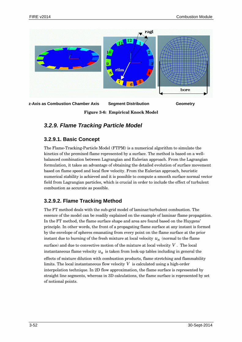
FIRE v2014 Combustion Module
3-52 30-Sept-2014
z-Axis as Combustion Chamber Axis Segment Distribution Geometry
Figure 3-6: Empirical Knock Model
3.2.9. Flame Tracking Particle Model
3.2.9.1. Basic Concept The Flame-Tracking-Particle Model (FTPM) is a numerical algorithm to simulate the kinetics of the premixed flame represented by a surface. The method is based on a well-balanced combination between Lagrangian and Eulerian approach. From the Lagrangian formulation, it takes an advantage of obtaining the detailed evolution of surface movement based on flame speed and local flow velocity. From the Eulerian approach, heuristic numerical stability is achieved and it is possible to compute a smooth surface normal vector field from Lagrangian particles, which is crucial in order to include the effect of turbulent combustion as accurate as possible.
3.2.9.2. Flame Tracking Method The FT method deals with the sub-grid model of laminar/turbulent combustion. The essence of the model can be readily explained on the example of laminar flame propagation. In the FT method, the flame surface shape and area are found based on the Huygens’ principle. In other words, the front of a propagating flame surface at any instant is formed by the envelope of spheres emanating from every point on the flame surface at the prior instant due to burning of the fresh mixture at local velocity nu (normal to the flame
surface) and due to convective motion of the mixture at local velocity V . The local instantaneous flame velocity nu is taken from look-up tables including in general the
effects of mixture dilution with combustion products, flame stretching and flammability limits. The local instantaneous flow velocity V is calculated using a high-order interpolation technique. In 2D flow approximation, the flame surface is represented by straight line segments, whereas in 3D calculations, the flame surface is represented by set of notional points.

Combustion Module FIRE v2014
30-Sept-2014 3-53
Turbulent Velocity Modeling
In the turbulent flow field, the mean energy release rate in the cell, Q , is composed of two
terms: energy release due to frontal combustion, fQ , and energy release due to volumetric
combustion, vQ .
Tinifrf uSQQ Σ= ρ , (3.163)
where frρ is the fresh mixture density, Q is the combustion heat, and summation is made
over all flame segments in the cell, i.e. index i relates to the i-th flame surface segment. The second term vQ is calculated by using the particle method as described below.
In the turbulent flow field, a pulsating velocity vector distorts the “mean” reactive (flame) surface by wrinkling it. The local instantaneous flame wrinkling can be taken into account by proper increasing the normal flame velocity, or in other words, by introducing a concept of local turbulent flame velocity Tu . The local turbulent flame velocity is defined as
nnT SSuu /= , (3.164)
where S is the surface area of the wrinkled flame at a given segment and nS is the surface
area of the equivalent “planar” flame.
In the theory of turbulent combustion, there are many correlations between Tu and nu .
E.g. one of the classical correlations has been found by Damköhler [3.19]:
′+⋅≈
nnT u
uuu 1 (3.165)
where u′ is the local turbulence intensity, related to the turbulent kinetic energy or to pulsating velocity correlations. Instead of equation (3.165) one can use any other available correlation for the turbulent flame velocity. In detailed investigations it was found that for calculations in engine combustion chambers e.g. the formulation by Guelder [3.33] delivers good physical results:
′+⋅≈
41
21
62.01v
luuuuu n
nnT (3.166)
One can apply the Huygens principle to model only the “mean” shape of the turbulent flame: each elementary portion of flame surface displaces in time due to burning of the fresh mixture at local velocity Tu (normal to the flame surface) and due to convective
motion of the mixture at local velocity V .
It stands to reason that the turbulent combustion model is also valid for the laminar combustion as a limiting case. This is one of the model advantages. Using the same model this feature allows to calculate the initial laminar flame kernel growth from the spark ignition with continuous transition to turbulent combustion.
FIRE v2014 Combustion Module
3-54 30-Sept-2014
Surface Evolution
Numerical methods for surface evolution are divided into two categories: front tracking methods based on Lagrangian frame and front capturing methods based on Eulerian frame. The algorithm used in FTPM method has an advantage of both Eulerian and Lagrangian approaches.
Method can stably compute geometrical properties and easily handle topological changes, but numerical schemes suffer from numerical diffusion and oscillations along the surface movement.
FTM is mainly based on the Lagrangian particle method in order to track characteristic information and it is well-balanced with the Eulerian method to obtain a surface normal vector field and reduce numerical instability caused by explicit particle movement. In an evolution of the surface from a given velocity and an initial particle location, the method consists of four steps: Computation of volume fraction, Computation of surface normal vectors, Re-seeding of particles, Movement of particles.
• Step 1: Computation of volume fraction
The volume fraction is an averaged information of representing the surface and it is used to compute the effect of the surface location caused by turbulent models in compressible Navier-Stokes equations. The computation of the volume fraction from given particles can be easily done by obtaining an averaged plane surface in each cell.
• Step 2: Computation of surface normal vectors
A normal vector field from the averaged surface does not have good quality to correctly present the surface geometry. This is because the continuity of the normal vector field is not guaranteed and the discontinuity is obviously caused by ignoring neighbor information and averaging locations of particles per cell. In order to avoid such a local disturbance, a reconstruction of a continuous global surface is proposed by an iterative scheme. The method quickly converges under the criterion of globally obtaining the surface close to previous particles. The surface normal vector field from the reconstructed surface is crucially used to apply different types of velocity field on each particle to evolve a surface in a turbulent combustion field. The reconstruction of a global surface structure based on particle locations corresponds to an Eulerian approach.
• Step 3: Re-seeding of particles
There are two typical drawbacks of using a particle-based method to evolve a surface in a given velocity field: 1. To obtain a viscosity solution under an effect of shock and rarefaction and 2. to follow topological changes (breaking and merging). Main difficulties are caused by the hyperbolic nature of Lagrangian particle movement and the lack of explicit surface representation. It is rather simple to solve the first problem from re-seeding particles. But, it is not easy to decide where particles should be re-seeded in the computational domain. Interestingly, a solution of the first problem is related to the second issue. In order to resolve such problems, it is well-known that the Eulerian approach is highly potential and it is already done in Step 2 with a proposed algorithm.
Combustion Module FIRE v2014
30-Sept-2014 3-55
However, even though the globally reconstructed surface in Step 2 gives a good quality of the normal vector field, it may lose the quality of surface location tracked by particles along the characteristics because the algorithm works based on a global criterion and it is not difficult to recognize that the global criterion averages out the local property. Now, before re-seeding of particles, the globally reconstructed surface in Step 2 is locally moved in order to preserve the quality of characteristic information while surface normal vectors are preserved. Therefore, the valuable characteristic information from the Lagrangian approach is not deteriorated and the smooth surface normal from the Eulerian approach to present geometrical information in Step 2 can be still used.
• Step 4: Movement of particles
From Step 1 to Step 3, particles are re-seeded and the surface normal vector field is computed. In this step, particles are simply moved along an obtained velocity field which is a combination of flame velocity and turbulent fluid velocity.
3.2.9.3. Particle Method Pre-flame reactions
The ‘particle method’ PM allows continuous monitoring of pre-flame reactions. Within the method, a certain number of Lagrangian particles move in the pre-flame zone according to the local velocity vector. In each particle, the pre-flame reactions proceed at the rates determined by its instantaneous temperature and species concentrations. For determining the time and location of pre-flame auto-ignition a certain criterion is adopted. Such a criterion is usually based on the fixed rate of temperature rise in the particle, e.g., 107 or 108 K/s. When the auto-ignition criterion is met in one or several particles in the computational cell, all amount of fuel in this cell are burnt during one time step. This process corresponds to the fast reactions and volumetric combustion/explosion in pre-flame zone. The number of particles in the pre-flame zone can be less than the number of computational cells. For keeping the number density of particles at a reasonable level, consistent procedures of particle cloning and clustering have been developed. The pre-flame particles are traced until the entire geometry is traversed by the frontal or volumetric combustion.
Post-flame reactions
For monitoring pollutants (NOx, soot, etc.), the PM is also applied to the combustion products. When the flame passes a computational cell, this cell is automatically filled with n particles. For stoichiometric and fuel-rich mixtures, the new particles are assigned with the temperature, as well as fuel, nitrogen, water vapor, and carbon dioxide concentrations taken from the cell center, whereas the concentration of molecular oxygen, soot, CO and prompt NO are taken from look-up tables in the FT method. For fuel-lean mixtures, the new particles are assigned with the temperature from the cell center, whereas fuel, oxygen, nitrogen, water vapor, and carbon dioxide concentrations are calculated from the stoichiometric relationship assuming complete combustion, and the concentration of soot, CO and prompt NO is taken from look-up tables in the FT method. The mean values of pollutant mass fractions are then obtained by statistical averaging over all particles currently located in a given cell. In general, the PM implies the existence of both pre-flame and post-flame particles, which differ by a single index denoting their status. Depending on this index, a different set of kinetic equations is solved.
FIRE v2014 Combustion Module
3-56 30-Sept-2014
Kinetic database
The coupled FTPM algorithm is supplemented with the database of tabulated laminar flame velocities, prompt NO, flame soot and free oxygen, as well as flame CO for a given fuel–air mixture in the wide range of initial temperature, pressure, exhaust gas recirculation, as well as the reaction kinetics of pre-flame fuel oxidation. The detailed, reduced, and overall kinetic mechanisms of hydrocarbon (pre-flame) auto-ignition at ICE conditions for methane, ethanol, propane, n-heptane, iso-octane, n-decane, n-tetradecane, and n-heptane – iso-octane blends (PRF) have been developed and validated and the corresponding database has been constructed. Also, the kinetic database for (post-flame) pollutant formation (soot, thermal NO) at ICE conditions has been developed for these individual hydrocarbons and fuel blends. In combination with the flame velocity database for the FT method, these kinetic databases constitute a unique tool for advanced combustion simulation.
3.2.9.4. Spark Ignition Modeling The FT ignition model is based on differences in physics of flame propagation immediately after ignition and at a finite time after ignition. At the ignition stage the flame is known to develop from the small-size discharge channel through the phase of mixture ignition and flame formation. Combustion at this stage (from now on called initial stage) is mostly governed by local physico-chemical properties of the reactive mixture and by small-scale turbulence. In the fully developed turbulent flame (regular stage properly treated in the FT model), combustion is to a large extent governed by large-scale turbulence. Of course, there is a need in proper tailoring the initial and regular stages of flame propagation.
Physically, the turbulent flame in IC engine conditions is the highly wrinkled laminar flame. Therefore, one can use the classical expression for the turbulent flame velocity at such conditions:
m
tnt v
vuu += 1 (3.167)
where un is the laminar flame velocity, νt the turbulent (eddy) viscosity, νm and the molecular viscosity.
At the initial stage of flame propagation including ignition stage, when the flame kernel is small, the flame front can be wrinkled only by the low-energy flow velocity pulsations with the length scale less than the characteristic size (diameter) of flame kernel. In this case, all velocity pulsations of the larger scale play a role of the mean convective flow displacing the flame kernel as a whole. Since at the initial stage the flame size in URANS simulations is
on the order of grid spacing, it appears that uu′ and ul are in general the unresolved
pulsating velocity and length scale (this is the reason for the subscript u which means “unresolved”). Thus at the initial stage of flame propagation (at time t>tign, tign is the time of ignition triggering), the turbulent (eddy) viscosity in equation (3.167) should be estimated based on the time dependent unresolved pulsating velocity of scale lower than the instantaneous equivalent flame kernel diameter, i.e.,
)()(~)( tltutv uut ′ at )()( tdtl fu ≤ . (3.168)
Combustion Module FIRE v2014
30-Sept-2014 3-57
Without loss of generality, one can assume that fu dl ≈and rewrite equation (3.168) as
fut duv ′~ (3.169)
To estimate uu′ , one can use the approach suggested in [3.31], which introduces the ratio
of unresolved-to-total turbulent kinetic energies kkf uk /= , where 2)2/3( uu uk ′≈ is the
unresolved turbulent kinetic energy and 2)2/3( uk ′= is the resolved turbulent kinetic
energy, whereas uu′ and u′ are the unresolved and resolved pulsating velocities,
respectively. According to [3.31], the ratio of unresolved-to-total turbulent kinetic energies depends upon the characteristic grid spacing ∆ as
3/21~
Λ∆
µCfk , (3.170)
where
ε/2/3k=Λ (3.171)
is the integral length scale of turbulence (ε is the turbulence dissipation rate), and 09.0=µC
is the constant in the ε−k model of turbulence. According to [3.3], relationship (3.170) can be applied to time dependent conditions once the time scale of
changes in kf is smaller than that of turbulence quantities. Because we are interested in
the unresolved turbulence on scale fd rather than of scale ∆ one can rewrite equation
(3.170) of [3.31] as
3/2
1~
Λ
fk
dC
fµ
(3.172)
Now, taking into account that 09.0=µC
and using equations (3.169) and (3.171), one
finally obtains for the turbulent flame velocity at the initial stage initu , of equation (3.156) the following relationship:
m
fn
m
initninit v
du
vv
uu3/43/1
,, 5.11~1
ε++= (3.173)
Physically, when the initial stage of turbulent flame propagation comes to an end, the flame velocity should be determined by the correlation available in the FT model for the regular stage of flame propagation, e.g., by the Guelder expression. This transition takes place at the time when ut,ini becomes larger than ut.
FIRE v2014 Combustion Module
3-58 30-Sept-2014
3.3. References [3.1] Ahmadi-Befrui, B., Gosman, A. D., Lockwood, R.C. and Watkins, A. P.
"Multidimensional Calculation of Combustion in an Idealized Homogeneous Charge Engine: A Progress Report." Society of Automotive Engineers (SAE) 810151, 1981.
[3.2] Ahmadi-Befrui, B. and Kratochwill, H. "Multidimensional Calculation of Combustion in a Loop-scavenged Two-stroke Cycle Engine." Proc. of the International Symposium on Diagnostics and Modeling of Combustion in Internal Combustion Engines. The Japanese Society of Mechanical Engineers. Tokyo, 1990: 465-474
[3.3] Basara, B., Krajnovic, S., Girimaji, S. and Pavlovic, Z. “Near-wall formulation of the Partially Averaged Navier-Stokes turbulence model”, AIAA Journal, Vol. 49, pp. 2627-2636.
[3.4] Blint, R.J. "The Relationship of the Laminar Flame Width to Flame speed." Combustion Sci. and Tech. 49 (1986): 79-92.
[3.5] Bogdan, Ž. and Duić, N. “The Mathematical Model of the Steam Generator Combustion Chamber”, Proc 24th Symposium KoREMA, Zagreb, pg. 77, 1992.
[3.6] Bogdan, Ž., Duić, N. and Schneider, D.R. “Three-dimensional Simulation of the Performance of an Oil-fired Combustion Chamber”, Proc. of the 2nd European Thermal Sciences & 14th UIT National Heat Transfer Conference, Rome,1493-1495,1996.
[3.7] Bogensperger, M. "A Comparative Study of Different Calculation Approaches for the Numerical Simulation of Thermal NO Formation." Diss. U. Graz, 1996.
[3.8] Boie, W. "Vom Brennstoff zum Rauchgas. Feuerungstechnisches Rechnen mit Brennstoffkenngrößen und seine Vereinfachung mit Mitteln der Statistik." Leipzig: Teubner, 1957.
[3.9] Borghi, R., Delamare, L. and Gonzales, M. "The Modeling and Calculation of a Turbulent Flame Propagation in a Closed Vessel." CORIA - URA, No. 230 CNRS - Faculte des Sciences de Rouen.
[3.10] Brandstätter, W. and Johns, R.J.R. "The Application of a Probability Method to Engine Combustion Modeling." IMechE C58/83, 1983.
[3.11] Candel, S. and Poinsot, T. "Flame Stretch and the Balance Equation for the Flame Area." Combust. Sci. and Tech. 70 (1990): 1-15.
[3.12] Cant, R. S. and Bray, K.N.C. "Strained Laminar Flamelet Calculation of Premixed Turbulent Combustion in a Closed Vessel." 22nd International Symposium on Combustion. Pittsburgh: The Combustion Institute, 1990.
[3.13] Charlette F., Meneveau C. and Veynante D., “A power-law flame wrinkling model for LES of premixed turbulent combustion PART I: non-dynamic formulation and initial tests”, Combustion and Flame, Vol. 131, No. 1-2, pp. 159-180, 2002
[3.14] Colin, O., Benkenida, A. and Angelberger, C. "3D Modeling of Mixing, Ignition and Combustion Phenomena in Highly Stratified Gasoline Engines", Oil & Gas Science and Technology - Rev IFP, 58(1), 47-62 (2003)
Combustion Module FIRE v2014
30-Sept-2014 3-59
[3.15] Colin O., Duclos F., Veynante D. and Poinsot T., “A thickened flame model for large eddy simulations of turbulent premixed combustion”, Phys. Fluids, Vol. 12, No. 7, pp. 1843-1863, 2000
[3.16] Colin O. and Truffin, K., "A spark ignition model for large eddy simulation based on an FSD transport equation (ISSIM-LES)," Proceeding of the Combustion Institute , vol. 33, pp. 3097-3104, 2011.
[3.17] Cox, R. and Cole, J. "Chemical Aspects of the Autoignition of Hydrocarbon-Air Mixtures." Combustion Flame 60 (1985): 109-123.
[3.18] Curl, R.L. "Dispersed phase mixing: 1. Theory and Effects in Simple Reactors." AICHE Journal 9 (1963): 175-181.
[3.19] Damkoehler G. Der Einfuss der Turbulenz auf die Flammen-geschwindigkeit in Gasgemischen. Zs Electrochemie 1940; 6: 601–52.
[3.20] Delhaye, B. and Cousyn, B. "Computation of Flow and Combustion in Spark Ignition Engine and Comparison with Experiment." SAE 961960, 1996.
[3.21] Deuflhard, P. and Nowak, U. "Extrapolation Integrators for Quasilinear Implicit ODEs," In: Deuflhard, P., Engquist, B. (eds.): Large Scale Scientific Computing, Birkhaeuser, Prog. Sci. Comp. 7, (1987): 37-50.
[3.22] Douaud, A.M. and Eyzat, P. “Four Octane Number Method for Predicting the Anti-Knock Behavior of Fuels and Engines”, SAE 780080,1978
[3.23] Duclos, J.M., Veynante, D. and Poinsot, T. "A Comparison of Flamelet Models for Premixed Turbulent Combustion." Combustion and Flame 95 (1993): 101-117.
[3.24] Duclos, J. M., Zolver, M. and Baritaud, T. "3D Modeling of Combustion for DI-SI Engines, Oil & Gas Science and Technology". -Rev. IFP, Vol. 54 (1999), No. 2, pp. 259-264
[3.25] Duclos, J. M., Zolver, M. and Baritaud, T. "3D Modeling of Combustion for DI-SI Engines", Oil & Gas Science and Technology -Rev. IFP, 54(2), 259-264 (1999)
[3.26] Duclos, J.M. and Colin, O. "Arc and Kernel Tracking Ignition Model for 3D Spark-Ignition Engine Calculations", COMODIA, 343-350 (2001)
[3.27] Ehrig, R., Nowak, U., Oeverdieck, L. and Deuflhard, P. "Advanced Extrapolation Methods for Large Scale Differential Algebraic Problems." In: High Performance Scientific and Engineering Computing, Bungartz, H. J., Durst, F. and Zenger Chr. (eds.), Lecture Notes in Computational Science and Engineering, Springer Vol 8, (1999): 233-244.
[3.28] el Tahry, S.H. "A Turbulent Combustion Model for Homogeneous Charge Engines." Combustion Flame 79 (1990): 122-140.
[3.29] Fan, L., Li, G., Han, Z. and Reitz, R.D. "Modeling fuel preparation and stratified combustion in a gasoline direct injection engine", SAE 01-0175, 1999.
[3.30] Fisch, A., Read, A., Affleck, W. and Haskell, W. "The Controlling Role of Cool Flames in Two-Stage Ignition." Combustion Flame 13 (1969): 39-49.
FIRE v2014 Combustion Module
3-60 30-Sept-2014
[3.31] Girimaji, S. Srinivasan, R. and Jeong, E. “PANS turbulence models for seamless transition between RANS and LES; fixed point analysis and preliminary results”. ASME paper FEDSM45336, 2003.
[3.32] Görner, K. Technische Verbrennungssysteme, Grundlagen, Modelbildung, Simulation. Springer Verlag Berlin Heidelberg, 1991.
[3.33] Guelder O.L. “Turbulent premixed flame propagation models for different combustion regimes Symposium (International) on Combustion“, Volume 23, Issue 1, 1991, Pages 743-750
[3.34] Halstead, M., Kirsch, L., Prothero, A. and Quinn, O. "A Mathematical Model for Hydrocarbon Auto-Ignition at High Pressures." Proc. Royal Society of London, A246, 1975: 515-538
[3.35] Halstead, M., Kirsch, L. and Quinn, C. "The Autoignition of Hydrocarbon Fueld at High Temperatures and Pressures - Fitting of a Mathematical Model." Combustion Flame 30 (1977): 45-60.
[3.36] Heywood, J. B. Internal Combustion Engine Fundamentals. McGrawHill Book Company, Second Series, 1988.
[3.37] Hioyasu, H., and Nishida, K. “Simplified Three Dimensional Modeling of Mixture Formation and Combustion in a DI Diesel Engine.” SAE 890269, 1989.
[3.38] Jones, W.P. and Lindstedt, R.P. "Global Reaction Schemes for Hydrocarbon Combustion." Combustion and Flame 73 (1988): 233-249.
[3.39] Kido, H., Nakahara, M. and Hashimoto, J. "A Turbulent Burning Velocity Model Taking Account of the Preferential Diffusion Effect". The Fourth International Symposium COMODIA 98, 1998.
[3.40] Kobayashi, H., Kawabata, Y., Maruta, K. "Experimental Study on General Correlation of Turbulent Burning Velocity at High Pressure." 27th International Symposium on Combustion. Pittsburgh: The Combustion Institute, 1998: 941-948.
[3.41] Kong, S.C., Han, Z. and Reitz, R.D. ”The Development and Application of a Diesel Ignition and Combustion Model for Multidimensional Engine Simulation.” SAE 950278, 1995.
[3.42] Lafossas, F.A., Castagne, M., Dumas, J.P. and Henriot, S. “Development and Validation of a Knock Model in Spark Ignition Engines Using a CFD code”, SAE 2002-01-2701, 2002.
[3.43] Maas, U. and Pope, S. B. "Simplifying Chemical Kinetics; Intrinsic low-dimensional Manifolds in Composition Space." Combustion and Flame 88 (1992): 239-264.
[3.44] Magnussen, B.F. and Hjertager, B.H. "On mathematical modeling of turbulent combustion with special emphasis on soot formation and combustion." Sixteenth International Symposium on Combustion. Pittsburgh: The Combustion Institute, 1977.
[3.45] Meintjes, K. and Morgan, A.P. "Element Variables and the Solution of Complex Chemical Equilibrium Problems," GMR-5827, General Motors Research Laboratories, Michigan, 1987.
[3.46] Meneveau, C. and Poinsot, T. "Stretching and Quenching of Flamelets in Premixed Turbulent Combustion." Combustion Flame 86 (1991): 311-332.

Combustion Module FIRE v2014
30-Sept-2014 3-61
[3.47] Meneveau, C. and Sreenivasan, K.R. "The Multifractal Nature of Turbulent Energy Dissipation." Journal of Fluid Mechanics 224 (1991): 429-484.
[3.48] Metghalchi, M. and Keck, J.C. "Burning Velocities of Mixtures of Air with Methanol, Isooctane and Indolene at High Pressure and Temperature." Combustion and Flame 48 (1982): 191-210.
[3.49] Poinsot, T., Veynante, D. and Candel, S. "Quenching Processes and Premixed Turbulent Combustion Diagrams." Journal of Fluid Mechanics 228 (1991): 561-606.
[3.50] Pope, S.B. "A Monte Carlo Method for the PDF Equations of Turbulent Flow." MIT-EL 80-012.
[3.51] Pope, S.B. "PDF Methods for Turbulent Reactive Flows." Prog. Energy Combustion Science 11 (1985).
[3.52] Pope, S. B. and Cheng, W. K. "The Stochastic Flamelet Model of Turbulent Premixed Combustion." 22nd International Symposium on Combustion. Pittsburgh: The Combustion Institute, 1990.
[3.53] Richard S., Colin O., Vermorel O., Benkenida A., Angelberger C. and Veynante D., “Towards large eddy simulation of combustion in spark ignition engines”, Proceedings of the Combustion Institute, Vol. 31, No. 1, pp. 3059-3066, 2007
[3.54] Schäpertöns, H. and Lee, W. "Multidimensional Modeling of Knocking Combustion in SI Engines." SAE 850502, 1985.
[3.55] Spalding, D. B. Combustion and Mass Transfer. Oxford: Pergamon Press, 1979.
[3.56] Tatschl, R., Pachler, K., Fuchs, H., and Almer, W. "Multidimensional Simulation of Diesel Engine Combustion - Modeling and Experimental Verification." Proceedings of the Fifth Conference 'The Working Process of the Internal Combustion Engine'. Graz, Austria, 1995.
[3.57] Theobald, M. and Cheng, W. "A Numerical Study of Diesel Ignition." ASME 87-FE-2, 1987.
[3.58] Zeldovich, Y. B., Sadovnikov, P. Y. and Frank-Kamenetskii, D. A. Oxidation of Nitrogen in Combustion. Translation by M. Shelef, Academy of Sciences of USSR, Institute of Chemical Physics, Moscow-Leningrad, 1947.
3.4. Related Publications [3.59] Brandstätter, W., Pitcher, G., Tatschl, R. and Winklhofer, E. "Modeling of
Homogeneous-Charge Combustion in SI Engines." MTZ Worldwide - Motortechnische Zeitschrift 58:2(1997).
[3.60] Cartellieri, W., Chmela, F., Kapus, P. and Tatschl, R. "Mechanisms Leading to Stable and Efficient Combustion in Lean Burn Gas Engines." Proceedings International Symposium COMODIA 94, The Japan Society of Mechanical Engineers, 1994: 17-32.
[3.61] Frolov, S.M., Suffa, M., Tatschl, R. and Wolanski, P. "3D Modeling of Pulsed Jet Combustion." Zel'Dovich Memorial "Int. Conf. on Combustion", Moscow, Russia, 1994.
FIRE v2014 Combustion Module
3-62 30-Sept-2014
[3.62] Pachler, K., Tatschl, R., Fuchs, H. and Schwarz, W. "A Three-Dimensional Simulation of Diesel Combustion – Modeling and Experimental Validation." International Congress " Le moteur diesel – Evolutions et mutations", Lyon, France, 1996.
[3.63] Priesching, P., Wanker, R., Cartellieri, P. and Tatschl, R. “CFD Modeling of HCCI Engine Combustion – Validation and Application”, ICE 2003 Conference, Naples 2003.
[3.64] Priesching, P. Ramusch G., Ruetz J. and Tatschl, R. “3D-CFD Modeling of Conventional and Alternative Diesel Combustion and Pollutant Formation – A Validation Study”, JSAE F&L 2007, JSAE 20077285, SAE 2007-01-1907
[3.65] Priesching, P. and Poredos, A. “Premixed IC Engine Combustion Simulation Applying a Novel Type of Flame Tracking Approach”, International Multidimensional Engine Modeling User’s Group Meeting at the SAE Congress, 2014
[3.66] Tatschl, R. and Brandstätter, W. "Multidimensional Calculation of Spark Flame Initiation by Adopting a Generic Hydrocarbon Kinetic Scheme." Computational Methods in Applied Sciences. Ch. Hirsch (Ed.) Elsevier Publishers B.V., 1992: 283-293.
[3.67] Tatschl, R. "A Multi-Scalar PDF Method for SI Engine Combustion Simulation." Proceedings of the 11th Symposium on Turbulent Shear Flows. Grenoble, 1997.
[3.68] Tatschl, R., Bogensperger, M. and Riediger, H. "Current Status and Future Developments of FIRE Combustion Models." Proceedings of the 3rd International FIRE User Meeting. Graz, Austria, 1997.
[3.69] Tatschl, R., Bogensperger, M. and Riediger, H. "Modeling Spray Combustion in Diesel Engines." 22nd CIMAC International Congress on Combustion Engines, Copenhagen, 1998.
[3.70] Tatschl, R., Fuchs, H. and Brandstätter, W. "Experimentally Validated Multi-Dimensional Simulation of Mixture Formation and Combustion in Gasoline Engines." IMechE C499/050, 1996.
[3.71] Tatschl, R., Gabriel, H.P. and Priesching, P. "FIRE – A Generic CFD Platform for DI Diesel Engine Mixture Formation and Combustion Simulation." International Multidimensional Modeling User's Group Meeting at the SAE Congress. Detroit, U.S.A., 2001.
[3.72] Tatschl, R., v. Künsberg Sarre, Ch., Pachler, K., Schneider, J. and Winklhofer, E. "Multidimensional Simulation of Gasoline Direct Injection Engines." Society of Automotive Engineers of Japan, 9932593, 1999.
[3.73] Tatschl, R., v. Künsberg Sarre, Ch., Priesching, P. and Putz, N. "A Comprehensive CFD Workflow for the Modeling of Gasoline DI Engines." The 1st National Congress on Fluids Engineering. Muju Resort, Korea, 2000.
[3.74] Tatschl, R., Pachler, K. and Winklhofer, E. "A Comprehensive DI Diesel Combustion Model for Multidimensional Engine Simulation." Proceedings International Symposium COMODIA 98, The Japan Society of Mechanical Engineers, 1998: 141-148.
[3.75] Tatschl, R. and Riediger, H. "PDF Modeling of Stratified Charge SI Engine Combustion." SAE 981464, 1998.

Combustion Module FIRE v2014
30-Sept-2014 3-63
[3.76] Tatschl, R., Riediger, H. and Bogensperger, M. "Multidimensional Simulation of Spray Combustion and Pollutant Formation in a Medium Speed Marine Diesel Engine." FISITA World Automotive Congress. Paris, 1998: 739-752.
[3.77] Tatschl, R., Riediger, H. and Fuchs, H. "A Multi-Scalar PDF Method for Inhomogeneous-Charge SI Engine Combustion Simulation." Advanced Computation & Analysis of Combustion. G.D. Roy, S.M. Frolov, P. Givi (Editors). Moscow: ENAS Publishers (1997).
[3.78] Tatschl, R., Riediger, H., v. Künsberg Sarre, Ch., Putz, N. and Kickinger, F. "Rapid Meshing and Advanced Physical Modeling for Gasoline DI Engine Application." International Multidimensional Engine Modeling User's Group Meeting at the SAE Congress. Detroit, U.S.A., 2000.
[3.79] Tatschl, R., Riediger, H., v. Künsberg Sarre, Ch., Putz, N. and Kickinger, F. "Fast Grid Generation and Advanced Physical Modeling – Keys to Successful Application of CFD to Gasoline DI Engine Analysis." ImechE. London, U.K. 2000.
[3.80] Tatschl, R., Wieser, K. and Reitbauer, R. "Multidimensional Simulation of Flow Evolution, Mixture Preparation and Combustion in a 4-Valve SI Engine." Proceedings International Symposium COMODIA 94, The Japan Society of Mechanical Engineers, 1994: 139-149.
[3.81] Tatschl, R., Wiesler, B., Alajbegovic, A. and v. Künsberg Sarre, Ch. "Advanced 3D Fluid Dynamic Simulation for Diesel Engines." Thiesel 2000. Valencia, Spain, 2000.
[3.82] Wieser, K., Versaevel, P. and Motte, P. "A New 3D Model for Vaporizing Diesel Sprays Based on Mixing-Limited Vaporization." SAE 2000-01-0949, 2000.
[3.83] Winklhofer, E., Fraidl, G.K. and Tatschl, R. "Flame Visualization in Gasoline Engines - New Tools in Engine Development." IPC-8 Technical Paper No. 9530850, Society of Automotive Engineers of Japan, Inc., 1995.

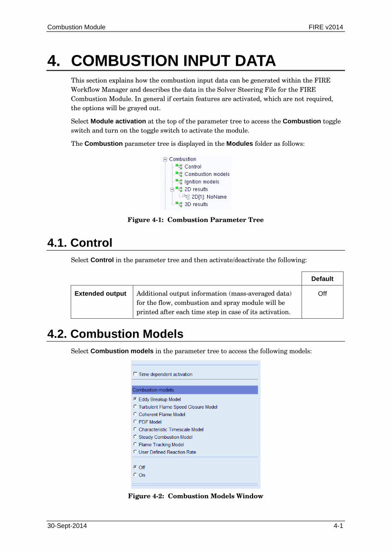
Combustion Module FIRE v2014
30-Sept-2014 4-1
4. COMBUSTION INPUT DATA This section explains how the combustion input data can be generated within the FIRE Workflow Manager and describes the data in the Solver Steering File for the FIRE Combustion Module. In general if certain features are activated, which are not required, the options will be grayed out.
Select Module activation at the top of the parameter tree to access the Combustion toggle switch and turn on the toggle switch to activate the module.
The Combustion parameter tree is displayed in the Modules folder as follows:
Figure 4-1: Combustion Parameter Tree
4.1. Control Select Control in the parameter tree and then activate/deactivate the following:
Default
Extended output Additional output information (mass-averaged data) for the flow, combustion and spray module will be printed after each time step in case of its activation.
Off
4.2. Combustion Models Select Combustion models in the parameter tree to access the following models:
Figure 4-2: Combustion Models Window
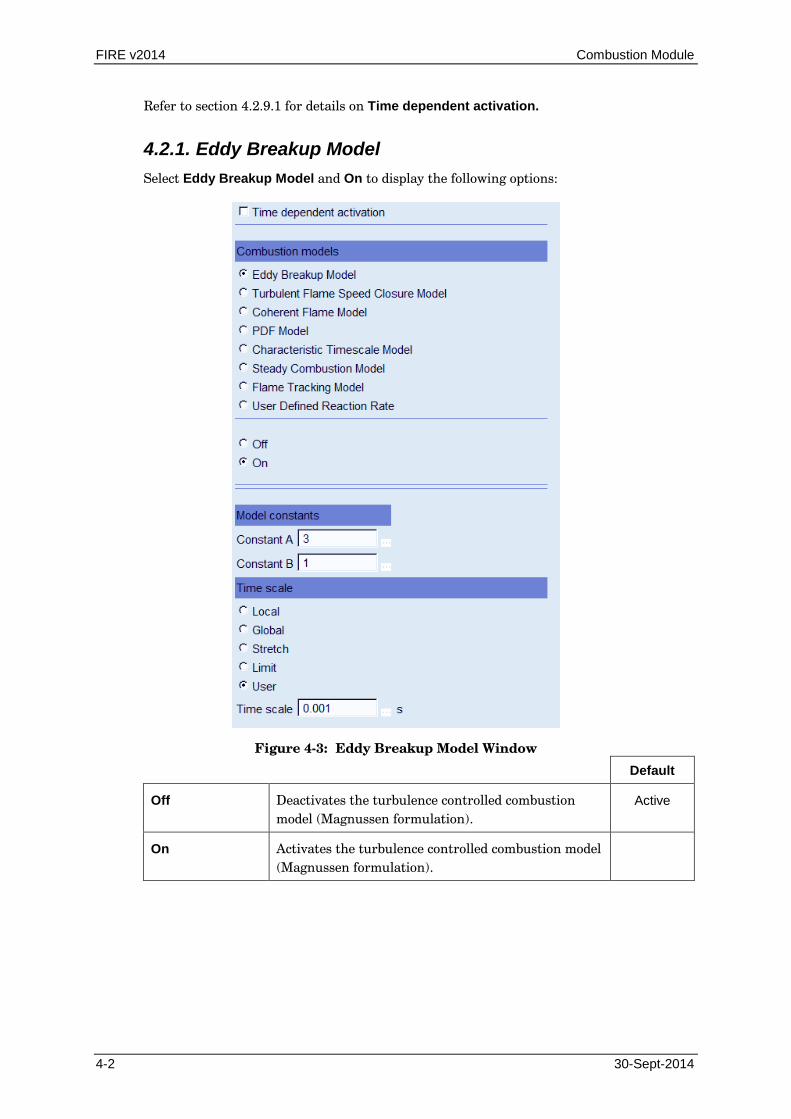
FIRE v2014 Combustion Module
4-2 30-Sept-2014
Refer to section 4.2.9.1 for details on Time dependent activation.
4.2.1. Eddy Breakup Model Select Eddy Breakup Model and On to display the following options:
Figure 4-3: Eddy Breakup Model Window
Default
Off Deactivates the turbulence controlled combustion model (Magnussen formulation).
Active
On Activates the turbulence controlled combustion model (Magnussen formulation).

Combustion Module FIRE v2014
30-Sept-2014 4-3
4.2.1.1. Model Constants Specification of the model constants A and B.
Default
Constant A The exact value for the constant A is problem specific and depends on the fuel and the detailed structure of the turbulent flow field. Thus it requires adjustment according to available experimental data. Common values for engine applications are between 3 and 25. An increase in A leads to an intensification of the turbulent reaction rate.
This is constant Cfu used in equation (3.2).
3
Constant B A value of about 0.5 – 1.0 has been found to be valid for B over a broad range of applications and should not be changed arbitrarily.
Recommended value for SI engine simulation: 0.5 Recommended value for CI (compression ignition) engine simulation: 1.0
This is constant CPr used in equation (3.2).
1
4.2.1.2. Time Scale Specifies the reaction time scale in the Magnussen combustion model. The options are described below:
SI engine combustion simulation is recommended to be performed using the global time scale option; spray combustion simulation should be performed using the local time scale definition.
Default
Local The depletion rate of the combustible mixture is taken to be proportional to the reaction time scale τR
determined by the local value of the ratio of the turbulence kinetic energy k and its dissipation rate ε.
Active
Global The depletion rate of the combustible mixture is taken to be proportional to the reaction time scale τR
determined by the global value of the ratio of the turbulence kinetic energy k and its dissipation rate ε
Stretch The depletion rate of the combustion mixture is determined by the local value of the ratio of k/ε corrected by a function considering the flame characteristics (thickness, velocity) and turbulence parameters (ITNFS model, refer to chapter 3.2.4.)
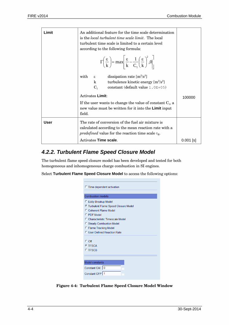
FIRE v2014 Combustion Module
4-4 30-Sept-2014
Limit An additional feature for the time scale determination is the local turbulent time scale limit. The local turbulent time scale is limited to a certain level according to the following formula:
ε
−ε
=
ε
Γ 0,kC
1k
maxk
2
1
with ε dissipation rate [m2/s3] k turbulence kinetic energy [m2/s2] C1 constant (default value 1.0E+05)
Activates Limit:
If the user wants to change the value of constant C1, a new value must be written for it into the Limit input field.
100000
User The rate of conversion of the fuel air mixture is calculated according to the mean reaction rate with a predefined value for the reaction time scale τR.
Activates Time scale.
0.001 [s]
4.2.2. Turbulent Flame Speed Closure Model The turbulent flame speed closure model has been developed and tested for both homogeneous and inhomogeneous charge combustion in SI engines.
Select Turbulent Flame Speed Closure Model to access the following options:
Figure 4-4: Turbulent Flame Speed Closure Model Window
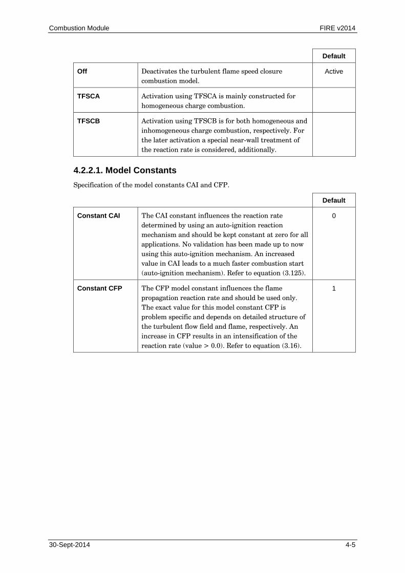
Combustion Module FIRE v2014
30-Sept-2014 4-5
Default
Off Deactivates the turbulent flame speed closure combustion model.
Active
TFSCA Activation using TFSCA is mainly constructed for homogeneous charge combustion.
TFSCB Activation using TFSCB is for both homogeneous and inhomogeneous charge combustion, respectively. For the later activation a special near-wall treatment of the reaction rate is considered, additionally.
4.2.2.1. Model Constants Specification of the model constants CAI and CFP.
Default
Constant CAI The CAI constant influences the reaction rate determined by using an auto-ignition reaction mechanism and should be kept constant at zero for all applications. No validation has been made up to now using this auto-ignition mechanism. An increased value in CAI leads to a much faster combustion start (auto-ignition mechanism). Refer to equation (3.125).
0
Constant CFP The CFP model constant influences the flame propagation reaction rate and should be used only. The exact value for this model constant CFP is problem specific and depends on detailed structure of the turbulent flow field and flame, respectively. An increase in CFP results in an intensification of the reaction rate (value > 0.0). Refer to equation (3.16).
1
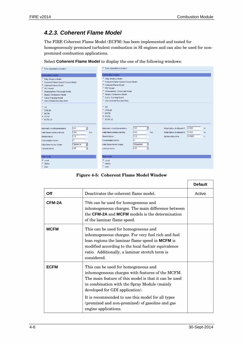
FIRE v2014 Combustion Module
4-6 30-Sept-2014
4.2.3. Coherent Flame Model The FIRE Coherent Flame Model (ECFM) has been implemented and tested for homogeneously premixed turbulent combustion in SI engines and can also be used for non-premixed combustion applications.
Select Coherent Flame Model to display the one of the following windows:
Figure 4-5: Coherent Flame Model Window
Default
Off Deactivates the coherent flame model. Active
CFM-2A This can be used for homogeneous and inhomogeneous charges. The main difference between the CFM-2A and MCFM models is the determination of the laminar flame speed.
MCFM This can be used for homogeneous and inhomogeneous charges. For very fuel rich and fuel lean regions the laminar flame speed in MCFM is modified according to the local fuel/air equivalence ratio. Additionally, a laminar stretch term is considered.
ECFM This can be used for homogeneous and inhomogeneous charges with features of the MCFM. The main feature of this model is that it can be used in combination with the Spray Module (mainly developed for GDI application).
It is recommended to use this model for all types (premixed and non-premixed) of gasoline and gas engine applications.
Combustion Module FIRE v2014
30-Sept-2014 4-7
ECFM-3Z The ECFM-3Z model can be used for both gasoline and diesel auto-ignition applications. This is the recommended choice.
If CFM-2A, MCFM or ECFM is selected, the following options are available:
Automatic model parameters
Automatic specification of the initial flame surface density, stretch and consumption factor can be selected for full (Correlations_FL) and part (Correlations_PL) load engine conditions. If this button is activated the following 3 parameters are automatically determined and cannot be changed by the user (grayed out). If this option is used only the Spherical ignition model is used.
Note: These correlations are derived for the ECFM using the Database correlations (tabulated flame speeds) for the laminar flame speed (to be set in the Initial Conditions) and are not recommended for other CFM models. The two options Correlations_FL and Correlations_PL can only be accessed if the Database option is activated for the laminar flame speed in the initial conditions part of the GUI.
Off
Initial flame surface density
Specification of the initial flame surface density within the ignition cells. This is a problem specific model constant (recommended value 100 – 500 [1/m]). This value influences the ignition delay. The higher the initial value the shorter the ignition delay.
Note: If ECFM and Aktim/ISSIM (Initial flame kernel shape, see below) are selected this option is meaningless and does not appear. If Automatic model parameters is activated, this option is meaningless and is grayed out (automatic determination).
300 [1/m]
Stretch factor This is a problem specific model constant (recommended value 1.0 - 4.0). An increase of the stretch factor leads to an intensification of the production of the flame surface density and hence in a shorter and faster combustion phase.
Note: If Automatic model parameters is activated, this option is meaningless and is grayed out (automatic determination).
1.6
Consumption factor
Model constant (recommended value 1.0) which should not be changed.
Note: If Automatic model parameters is activated, this option is meaningless and is grayed out (default value is used).
1
FIRE v2014 Combustion Module
4-8 30-Sept-2014
Combustion chamber cell selection
If Automatic model parameters is activated this button is visible where a cell selection for the combustion chamber can be selected.
Note: If this selection is not available a default value for the stretch factor of 1.6 is used.
Not visible
Initial flame kernel shape
Principally each ignition model can be used for each CFM model (see recommendation in the description of each model)
Spherical: This ignition model can be used for all CFM models (mainly recommended). In this model a spherical flame kernel is released using the ignition time, flame kernel radius and spark duration with the flame surface density specified in the FIRE Workflow Manager. The flame surface density is kept constant in the ignition cells over the spark duration.
Note: If Automatic model parameters is activated, this option is meaningless and is grayed out (default model is used).
Spherical
Spherical_Delay: This ignition model is mainly developed for the ECFM model (however AKTIM in connection with ECFM should be preferred, see below) and should not be used for the other CFM models. A specific time for the deposition of the flame kernel after spark timing is calculated. Additionally, the spherical flame radius and the flame surface density in the ignition cells are automatically determined. The only specification in the FIRE Workflow Manager is the ignition time and the activation of Spherical_Delay. This model can also be activated for the other CFM models (not recommended) but can lead to no flame kernel deposition (no ignition). The "Ellipsoidal" is similar to the "Spherical_Delay" model but in the latter model a spherical flame kernel is considered.
Ignition reference radius parameter: The user can modify the flame kernel radius to actual requirements.
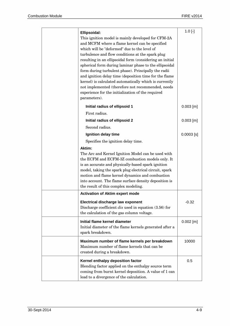
Combustion Module FIRE v2014
30-Sept-2014 4-9
Ellipsoidal: This ignition model is mainly developed for CFM-2A and MCFM where a flame kernel can be specified which will be "deformed" due to the level of turbulence and flow conditions at the spark plug resulting in an ellipsoidal form (considering an initial spherical form during laminar phase to the ellipsoidal form during turbulent phase). Principally the radii and ignition delay time (deposition time for the flame kernel) is calculated automatically which is currently not implemented (therefore not recommended, needs experience for the initialization of the required parameters).
1.0 [-]
Initial radius of ellipsoid 1
First radius.
Initial radius of ellipsoid 2
Second radius.
Ignition delay time
Specifies the ignition delay time.
Aktim: The Arc and Kernel Ignition Model can be used with the ECFM and ECFM-3Z combustion models only. It is an accurate and physically-based spark ignition model, taking the spark plug electrical circuit, spark motion and flame kernel dynamics and combustion into account. The flame surface density deposition is the result of this complex modeling.
0.003 [m]
0.003 [m]
0.0003 [s]
Activation of Aktim expert mode
Electrical discharge law exponent Discharge coefficient dis used in equation (3.56) for the calculation of the gas column voltage.
-0.32
Initial flame kernel diameter Initial diameter of the flame kernels generated after a spark breakdown.
0.002 [m]
Maximum number of flame kernels per breakdown Maximum number of flame kernels that can be created during a breakdown.
10000
Kernel enthalpy deposition factor Blending factor applied on the enthalpy source term coming from burnt kernel deposition. A value of 1 can lead to a divergence of the calculation.
0.5
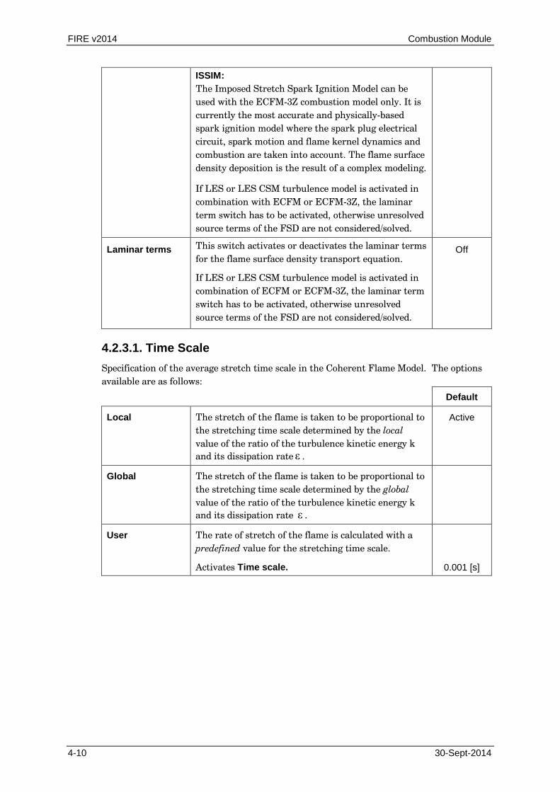
FIRE v2014 Combustion Module
4-10 30-Sept-2014
ISSIM: The Imposed Stretch Spark Ignition Model can be used with the ECFM-3Z combustion model only. It is currently the most accurate and physically-based spark ignition model where the spark plug electrical circuit, spark motion and flame kernel dynamics and combustion are taken into account. The flame surface density deposition is the result of a complex modeling.
If LES or LES CSM turbulence model is activated in combination with ECFM or ECFM-3Z, the laminar term switch has to be activated, otherwise unresolved source terms of the FSD are not considered/solved.
Laminar terms This switch activates or deactivates the laminar terms for the flame surface density transport equation.
If LES or LES CSM turbulence model is activated in combination of ECFM or ECFM-3Z, the laminar term switch has to be activated, otherwise unresolved source terms of the FSD are not considered/solved.
Off
4.2.3.1. Time Scale Specification of the average stretch time scale in the Coherent Flame Model. The options available are as follows:
Default
Local The stretch of the flame is taken to be proportional to the stretching time scale determined by the local value of the ratio of the turbulence kinetic energy k and its dissipation rate ε .
Active
Global The stretch of the flame is taken to be proportional to the stretching time scale determined by the global value of the ratio of the turbulence kinetic energy k and its dissipation rate ε .
User The rate of stretch of the flame is calculated with a predefined value for the stretching time scale.
Activates Time scale.
0.001 [s]

Combustion Module FIRE v2014
30-Sept-2014 4-11
4.2.3.2. ECFM-3Z Select the ECFM-3Z model to display the following options (gasoline and diesel auto-ignition mode):
Figure 4-6: ECFM-3Z Model Window
Figure 4-7: ECFM-3Z Model Window for Gasoline Engine Application
The parameters, factors and sub-models are the same as for ECFM and are described in the ECFM activation chapter 4.2.3.
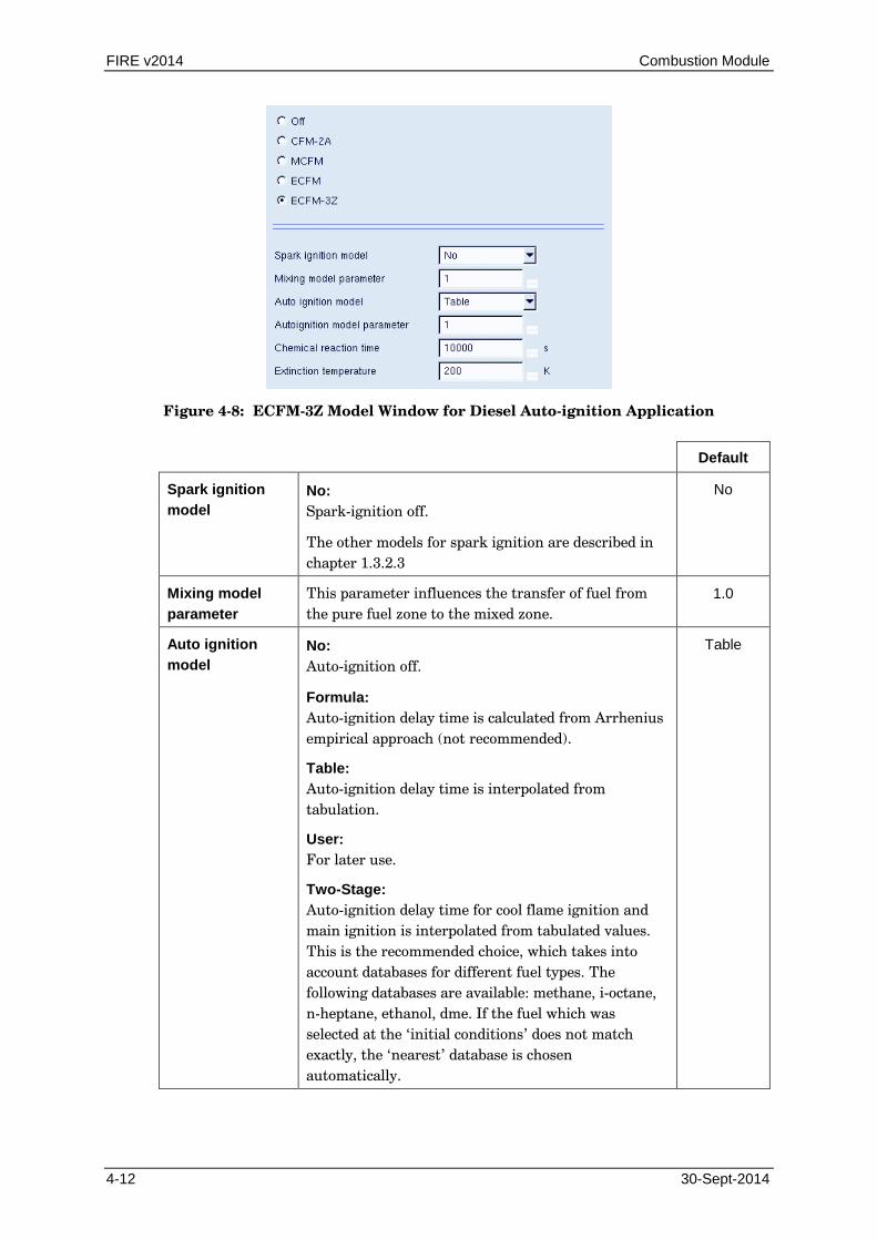
FIRE v2014 Combustion Module
4-12 30-Sept-2014
Figure 4-8: ECFM-3Z Model Window for Diesel Auto-ignition Application
Default
Spark ignition model
No: Spark-ignition off.
The other models for spark ignition are described in chapter 1.3.2.3
No
Mixing model parameter
This parameter influences the transfer of fuel from the pure fuel zone to the mixed zone.
1.0
Auto ignition model
No: Auto-ignition off.
Formula: Auto-ignition delay time is calculated from Arrhenius empirical approach (not recommended).
Table: Auto-ignition delay time is interpolated from tabulation.
User: For later use.
Two-Stage: Auto-ignition delay time for cool flame ignition and main ignition is interpolated from tabulated values. This is the recommended choice, which takes into account databases for different fuel types. The following databases are available: methane, i-octane, n-heptane, ethanol, dme. If the fuel which was selected at the ‘initial conditions’ does not match exactly, the ‘nearest’ database is chosen automatically.
Table
Combustion Module FIRE v2014
30-Sept-2014 4-13
Autoignition model parameter
This only works with the options ‘Table’ and ‘Two-stage’ for the ‘Auto-ignition model’. The inverse of this value is multiplied with the ignition delay time from the databases. This means that values larger than 1 are accelerating the ignition and vice versa.
1.0
Chemical reaction time
This value influences the rate of reaction of the fuel during premixed combustion and during auto-ignition.
1.0e+04
Extinction temperature
Temperature limit below which the fuel is transformed back from burnt status to unburned status.
When multiple injections are calculated, the recommended value is 1500 K or higher.
200.0
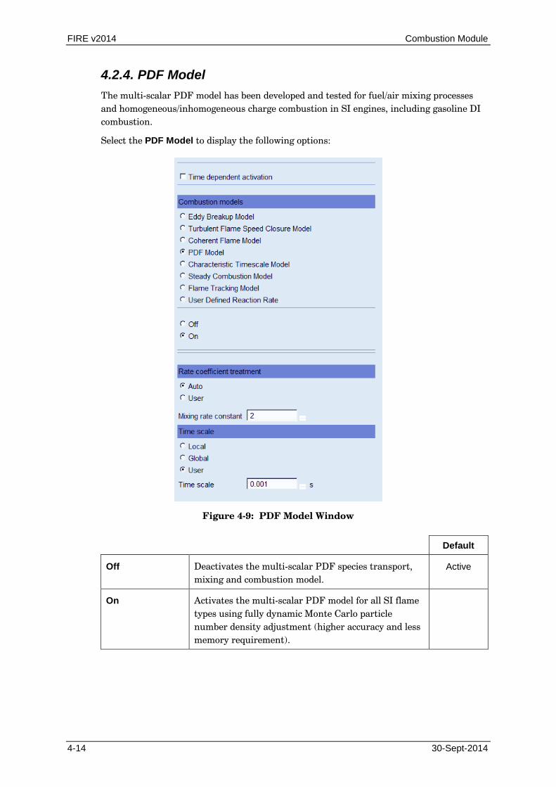
FIRE v2014 Combustion Module
4-14 30-Sept-2014
4.2.4. PDF Model The multi-scalar PDF model has been developed and tested for fuel/air mixing processes and homogeneous/inhomogeneous charge combustion in SI engines, including gasoline DI combustion.
Select the PDF Model to display the following options:
Figure 4-9: PDF Model Window
Default
Off Deactivates the multi-scalar PDF species transport, mixing and combustion model.
Active
On Activates the multi-scalar PDF model for all SI flame types using fully dynamic Monte Carlo particle number density adjustment (higher accuracy and less memory requirement).

Combustion Module FIRE v2014
30-Sept-2014 4-15
4.2.4.1. Rate Coefficient Treatment Specification of the Arrhenius reaction coefficients either by the user or automatically.
Default
Auto The coefficients are set automatically based on data of Westbrook and Dyer depending on the used fuel type.
Mixing rate constant:
Specifies the value of the mixing rate constant in the PDF transport equation.
Recommended value for engine applications 2.0 - 10.0. Changing the value weakly affects the ignition delay time but exhibits significant influence on the main combustion phase. Increasing the value reduces the duration of the main combustion phase.
2
User Specifies the pre-exponential factor and the activation energy of the chemical reaction rate expression in the PDF transport equation in addition to the mixing rate constant (Figure 4-10).
Mixing rate constant
Specifies the value of the mixing rate constant in the PDF transport equation.
Recommended value for engine applications 2.0 - 10.0. Changing the value weakly affects the ignition delay time but exhibits significant influence on the main combustion phase. Increasing the value reduces the duration of the main combustion phase.
Preexponential factor
Recommended value: 1.0E11. An increase of the value leads to a faster chemical reaction and hence (in the case of SI engine combustion) to a shortening of the ignition delay (i.e. time until 2 [%] mass fraction burnt). Depending on the ratios of the physical and chemical time scales, the value may also slightly affect the duration of the main combustion phase.
Activation energy
Recommended value: 1.8E08. A small decrease of the value results in a dramatic augmentation of the flame propagation velocity in premixed SI engine combustion, and hence, to a shortening of the ignition delay and the main combustion duration.
2
1e+11
1.8e+08
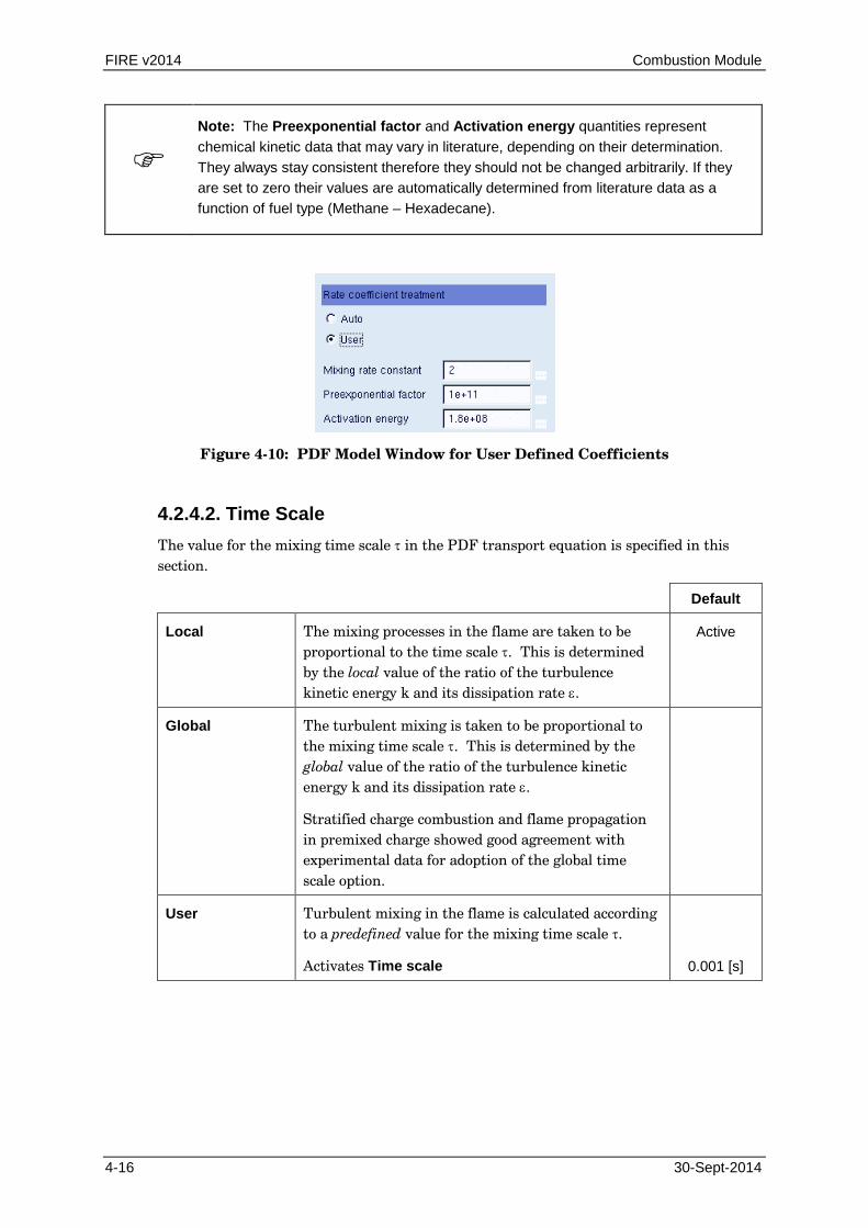
FIRE v2014 Combustion Module
4-16 30-Sept-2014
Note: The Preexponential factor and Activation energy quantities represent chemical kinetic data that may vary in literature, depending on their determination. They always stay consistent therefore they should not be changed arbitrarily. If they are set to zero their values are automatically determined from literature data as a function of fuel type (Methane – Hexadecane).
Figure 4-10: PDF Model Window for User Defined Coefficients
4.2.4.2. Time Scale The value for the mixing time scale τ in the PDF transport equation is specified in this section.
Default
Local The mixing processes in the flame are taken to be proportional to the time scale τ. This is determined by the local value of the ratio of the turbulence kinetic energy k and its dissipation rate ε.
Active
Global The turbulent mixing is taken to be proportional to the mixing time scale τ. This is determined by the global value of the ratio of the turbulence kinetic energy k and its dissipation rate ε.
Stratified charge combustion and flame propagation in premixed charge showed good agreement with experimental data for adoption of the global time scale option.
User Turbulent mixing in the flame is calculated according to a predefined value for the mixing time scale τ.
Activates Time scale
0.001 [s]
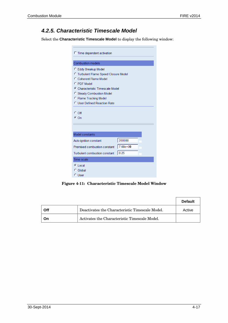
Combustion Module FIRE v2014
30-Sept-2014 4-17
4.2.5. Characteristic Timescale Model Select the Characteristic Timescale Model to display the following window:
Figure 4-11: Characteristic Timescale Model Window
Default
Off Deactivates the Characteristic Timescale Model. Active
On Activates the Characteristic Timescale Model.

FIRE v2014 Combustion Module
4-18 30-Sept-2014
4.2.5.1. Model Constants
Default
Auto ignition constant
This constant influences the auto ignition of the fuel. The larger the value, the faster the reaction (shorter ignition delay). This constant is used in equation IV of the SHELL model (section 3.2.8.1).
2e+05
Premixed combustion constant
This constant influences the laminar part of the combined reaction rate. The larger the value, the faster the reaction. This is constant A used in equation (3.142).
7.68e+09
Turbulent combustion constant
This constant influences the turbulent part of the combined reaction rule. The smaller the value, the faster the reaction. This is constant C2 used in equation (3.116).
0.25
4.2.5.2. Time Scale Specification of the reaction time scale in the Characteristic Timescale Model. The options are described as follows:
Default
Local The mixing processes in the flame are taken to be proportional to the time scale τ. This is determined by the local value of the ratio of the turbulence kinetic energy k and its dissipation rate ε.
Active
Global The turbulent mixing is taken to be proportional to the mixing time scale τ. This is determined by the global value of the ratio of the turbulence kinetic energy k and its dissipation rate ε.
User Turbulent mixing in the flame is calculated according to a predefined value for the mixing time scale τ.
Activates Time scale.
0.001 [s]
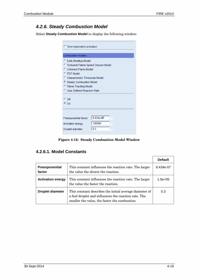
Combustion Module FIRE v2014
30-Sept-2014 4-19
4.2.6. Steady Combustion Model Select Steady Combustion Model to display the following window:
Figure 4-12: Steady Combustion Model Window
4.2.6.1. Model Constants
Default
Preexponential factor
This constant influences the reaction rate. The larger the value the slower the reaction.
9.434e-07
Activation energy This constant influences the reaction rate. The larger the value the faster the reaction.
1.0e+05
Droplet diameter This constant describes the initial average diameter of a fuel droplet and influences the reaction rate. The smaller the value, the faster the combustion.
0.3
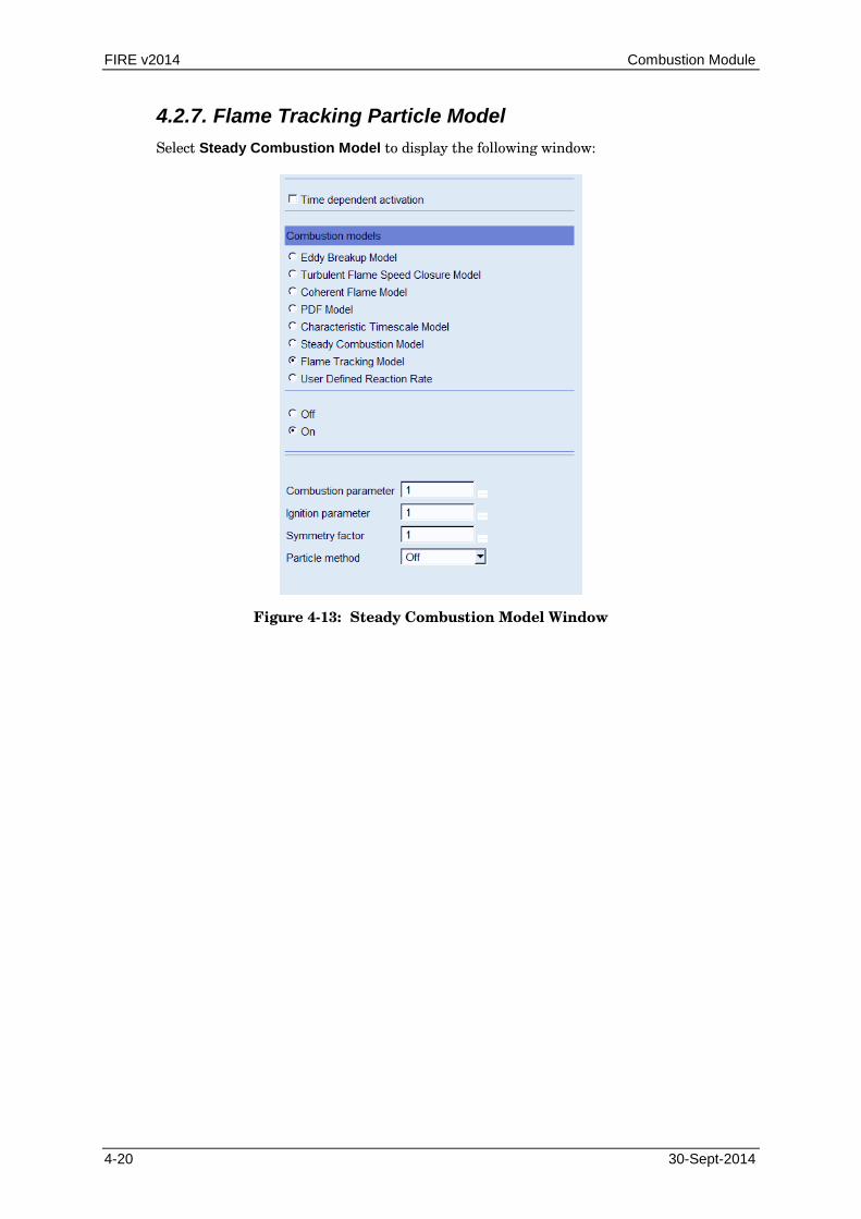
FIRE v2014 Combustion Module
4-20 30-Sept-2014
4.2.7. Flame Tracking Particle Model Select Steady Combustion Model to display the following window:
Figure 4-13: Steady Combustion Model Window
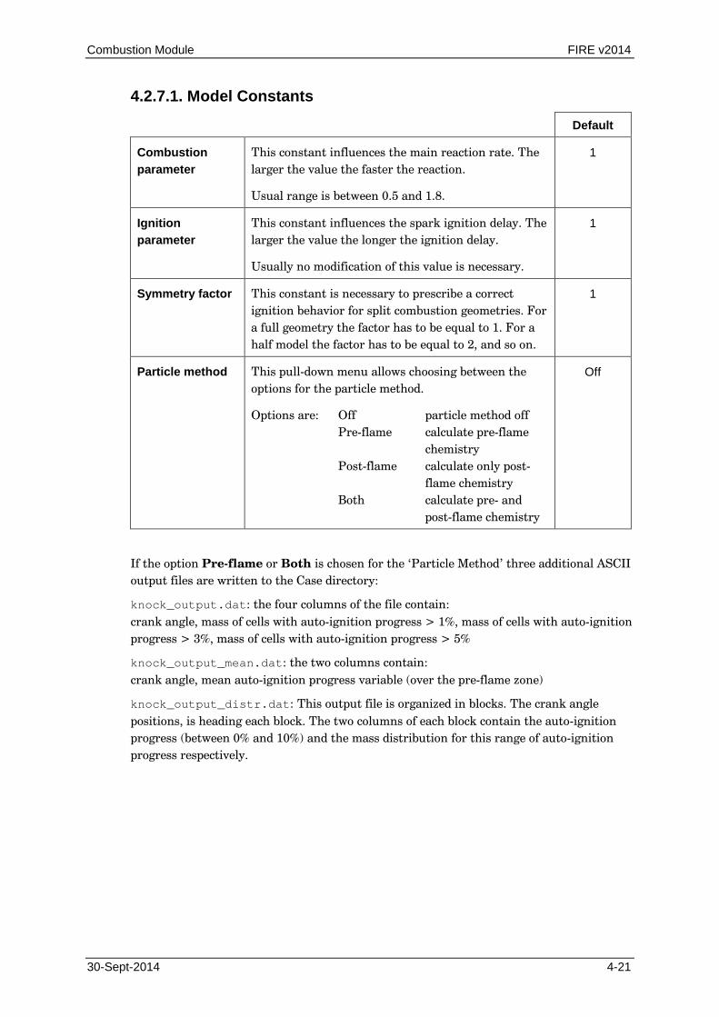
Combustion Module FIRE v2014
30-Sept-2014 4-21
4.2.7.1. Model Constants
Default
Combustion parameter
This constant influences the main reaction rate. The larger the value the faster the reaction.
Usual range is between 0.5 and 1.8.
1
Ignition parameter
This constant influences the spark ignition delay. The larger the value the longer the ignition delay.
Usually no modification of this value is necessary.
1
Symmetry factor This constant is necessary to prescribe a correct ignition behavior for split combustion geometries. For a full geometry the factor has to be equal to 1. For a half model the factor has to be equal to 2, and so on.
1
Particle method This pull-down menu allows choosing between the options for the particle method.
Options are: Off particle method off Pre-flame calculate pre-flame chemistry Post-flame calculate only post- flame chemistry Both calculate pre- and post-flame chemistry
Off
If the option Pre-flame or Both is chosen for the ‘Particle Method’ three additional ASCII output files are written to the Case directory:
knock_output.dat: the four columns of the file contain: crank angle, mass of cells with auto-ignition progress > 1%, mass of cells with auto-ignition progress > 3%, mass of cells with auto-ignition progress > 5%
knock_output_mean.dat: the two columns contain: crank angle, mean auto-ignition progress variable (over the pre-flame zone)
knock_output_distr.dat: This output file is organized in blocks. The crank angle positions, is heading each block. The two columns of each block contain the auto-ignition progress (between 0% and 10%) and the mass distribution for this range of auto-ignition progress respectively.

FIRE v2014 Combustion Module
4-22 30-Sept-2014
4.2.8. User Defined Reaction Rate The user can implement his own combustion model into a subroutine with the name "use_cctrat.f".
Select the User Defined Reaction Rate to access the following options:
Default
Off Deactivates the user defined reaction rate. Active
Explicit The subroutine is called before the SIMPLE loop.
Implicit The subroutine is called at each iteration within the SIMPLE loop.
4.2.9. Time Dependent Activation of Combustion
4.2.9.1. Combustion Models Select the Time dependent activation toggle switch and click on Table to show the following:
Figure 4-14: Time Dependent Activation of Combustion Models
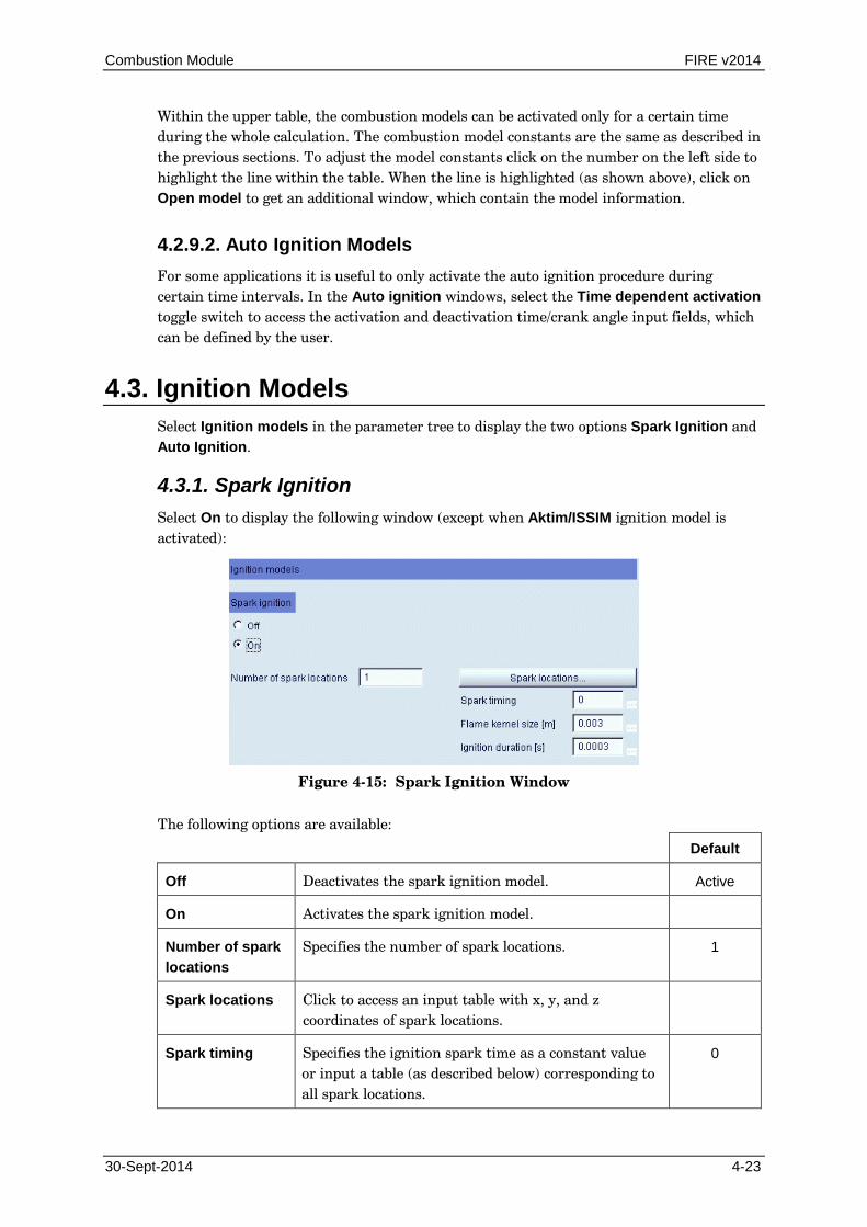
Combustion Module FIRE v2014
30-Sept-2014 4-23
Within the upper table, the combustion models can be activated only for a certain time during the whole calculation. The combustion model constants are the same as described in the previous sections. To adjust the model constants click on the number on the left side to highlight the line within the table. When the line is highlighted (as shown above), click on Open model to get an additional window, which contain the model information.
4.2.9.2. Auto Ignition Models For some applications it is useful to only activate the auto ignition procedure during certain time intervals. In the Auto ignition windows, select the Time dependent activation toggle switch to access the activation and deactivation time/crank angle input fields, which can be defined by the user.
4.3. Ignition Models Select Ignition models in the parameter tree to display the two options Spark Ignition and Auto Ignition.
4.3.1. Spark Ignition Select On to display the following window (except when Aktim/ISSIM ignition model is activated):
Figure 4-15: Spark Ignition Window
The following options are available:
Default
Off Deactivates the spark ignition model. Active
On Activates the spark ignition model.
Number of spark locations
Specifies the number of spark locations. 1
Spark locations Click to access an input table with x, y, and z coordinates of spark locations.
Spark timing Specifies the ignition spark time as a constant value or input a table (as described below) corresponding to all spark locations.
0

FIRE v2014 Combustion Module
4-24 30-Sept-2014
Flame kernel size [m]
Specifies the flame kernel radius as a constant value or input a table (as described below) corresponding to all spark locations.
Note: This value is meaningless if Aktim, ISSIM, Spherical_Delay or Ellipsoidal is selected as Initial flame kernel shape of the ECFM combustion model.
0.003
Ignition duration [s]
Specifies the ignition duration as a constant value or input a table (as described below) corresponding to all spark locations.
Note: This value is meaningless if Aktim, ISSIM, Spherical_Delay or Ellipsoidal is selected as Initial flame kernel shape of the ECFM combustion model.
0.0003
indicates that the user can input values in a table relating to the number of spark locations.
The following options are available:
1. Constant
This is the default setting and specifies that the parameter value entered in the field will remain constant for the entire simulation and for all spark locations.
2. Timing for Spark Timing Iteration.
Radius for Flame Kernel Size.
Duration for Ignition Duration.
The parameter input field is replaced by the relevant button mentioned above. Select it to open an input table where parameter values can be entered for each spark location.
When the Aktim ignition model is activated (ECFM Initial flame kernel shape) the window is displayed as shown. The options are described above.
Figure 4-16: Spark Ignition Window – Aktim ignition model
The window for the Aktim spark plug model looks like the following:
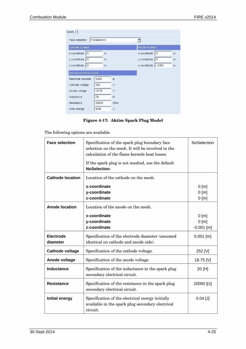
Combustion Module FIRE v2014
30-Sept-2014 4-25
Figure 4-17: Aktim Spark Plug Model
The following options are available
Face selection Specification of the spark plug boundary face selection on the mesh. It will be involved in the calculation of the flame kernels heat losses.
If the spark plug is not meshed, use the default NoSelection.
NoSelection
Cathode location Location of the cathode on the mesh.
x-coordinate y-coordinate z-coordinate
0 [m] 0 [m] 0 [m]
Anode location Location of the anode on the mesh.
x-coordinate y-coordinate z-coordinate
0 [m] 0 [m]
-0.001 [m]
Electrode diameter
Specification of the electrode diameter (assumed identical on cathode and anode side).
0.001 [m]
Cathode voltage Specification of the cathode voltage. 252 [V]
Anode voltage Specification of the anode voltage. 18.75 [V]
Inductance Specification of the inductance in the spark plug secondary electrical circuit.
20 [H]
Resistance Specification of the resistance in the spark plug secondary electrical circuit.
20000 [Ω]
Initial energy Specification of the electrical energy initially available in the spark plug secondary electrical circuit.
0.04 [J]

FIRE v2014 Combustion Module
4-26 30-Sept-2014
When the ISSIM ignition model is activated (only with the ECFM-3Z combustion model) the window for the ‘spark plug model’ is displayed as shown.
Figure 4-18: ISSIM Spark Plug Model
The following options are available
Spark location Location of the spark (centre between cathode and anode).
x-coordinate y-coordinate z-coordinate
0 [m] 0 [m] 0 [m]
Spark gap Specification of the distance between electrodes. 0.001 [m]
Electrode diameter
Specification of the electrode diameter. 0.001 [m]
Cathode voltage Specification of the cathode voltage. 252 [V]
Anode voltage Specification of the anode voltage. 18.75 [V]
Inductance Specification of the inductance in the spark plug secondary electrical circuit.
20 [H]
Resistance Specification of the resistance in the spark plug secondary electrical circuit.
20000 [Ω]

Combustion Module FIRE v2014
30-Sept-2014 4-27
Initial energy Specification of the electrical energy initially available in the spark plug secondary electrical circuit.
0.04 [J]
Symmetry factor Specification of the symmetry factor. For symmetry the factor is 2, for a sphere it is 1, for an eighth of a sphere it is 8.
1
4.3.2. Auto Ignition
Figure 4-19: Auto Ignition Window for Diesel
Default
Off Deactivates the auto ignition model. Active
4.3.2.1. Diesel Select Diesel to display the available options shown in Figure 4-19:
Diesel Activates the spray auto ignition model for diesel engine applications. Activates Reaction coefficient.
Reaction coefficient: Specifies the reaction rate coefficient for the formation of intermediate products in the Diesel self-ignition model (e.g. Dodecane: 1.e+07). Increasing/decreasing the value for the intermediate formation coefficient by one order of magnitude reduces/increases the ignition delay by approximately 0.1 -0.3 [ms], respectively, depending on the details of the application case under consideration.
Time dependent activation: Refer to section 4.2.9.2.
1e+07
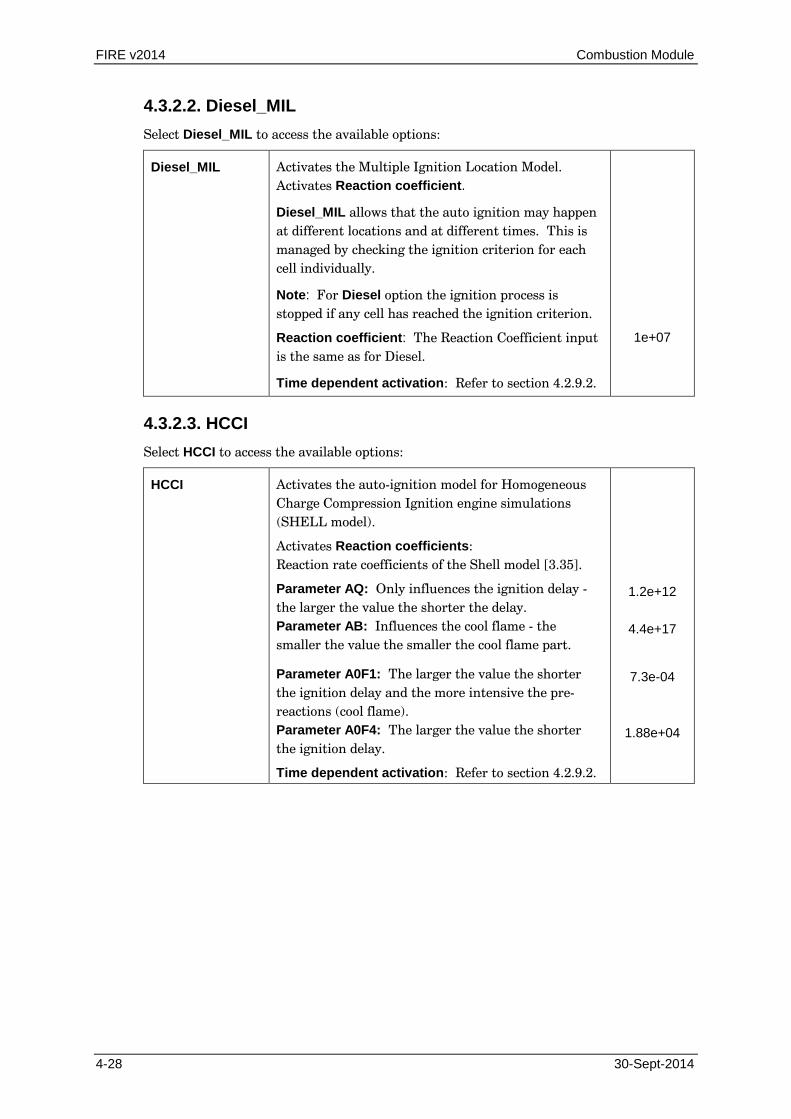
FIRE v2014 Combustion Module
4-28 30-Sept-2014
4.3.2.2. Diesel_MIL Select Diesel_MIL to access the available options:
Diesel_MIL Activates the Multiple Ignition Location Model. Activates Reaction coefficient.
Diesel_MIL allows that the auto ignition may happen at different locations and at different times. This is managed by checking the ignition criterion for each cell individually.
Note: For Diesel option the ignition process is stopped if any cell has reached the ignition criterion.
Reaction coefficient: The Reaction Coefficient input is the same as for Diesel.
Time dependent activation: Refer to section 4.2.9.2.
1e+07
4.3.2.3. HCCI Select HCCI to access the available options:
HCCI Activates the auto-ignition model for Homogeneous Charge Compression Ignition engine simulations (SHELL model).
Activates Reaction coefficients: Reaction rate coefficients of the Shell model [3.35].
Parameter AQ: Only influences the ignition delay - the larger the value the shorter the delay. Parameter AB: Influences the cool flame - the smaller the value the smaller the cool flame part.
1.2e+12
4.4e+17
Parameter A0F1: The larger the value the shorter the ignition delay and the more intensive the pre-reactions (cool flame). Parameter A0F4: The larger the value the shorter the ignition delay.
Time dependent activation: Refer to section 4.2.9.2.
7.3e-04
1.88e+04
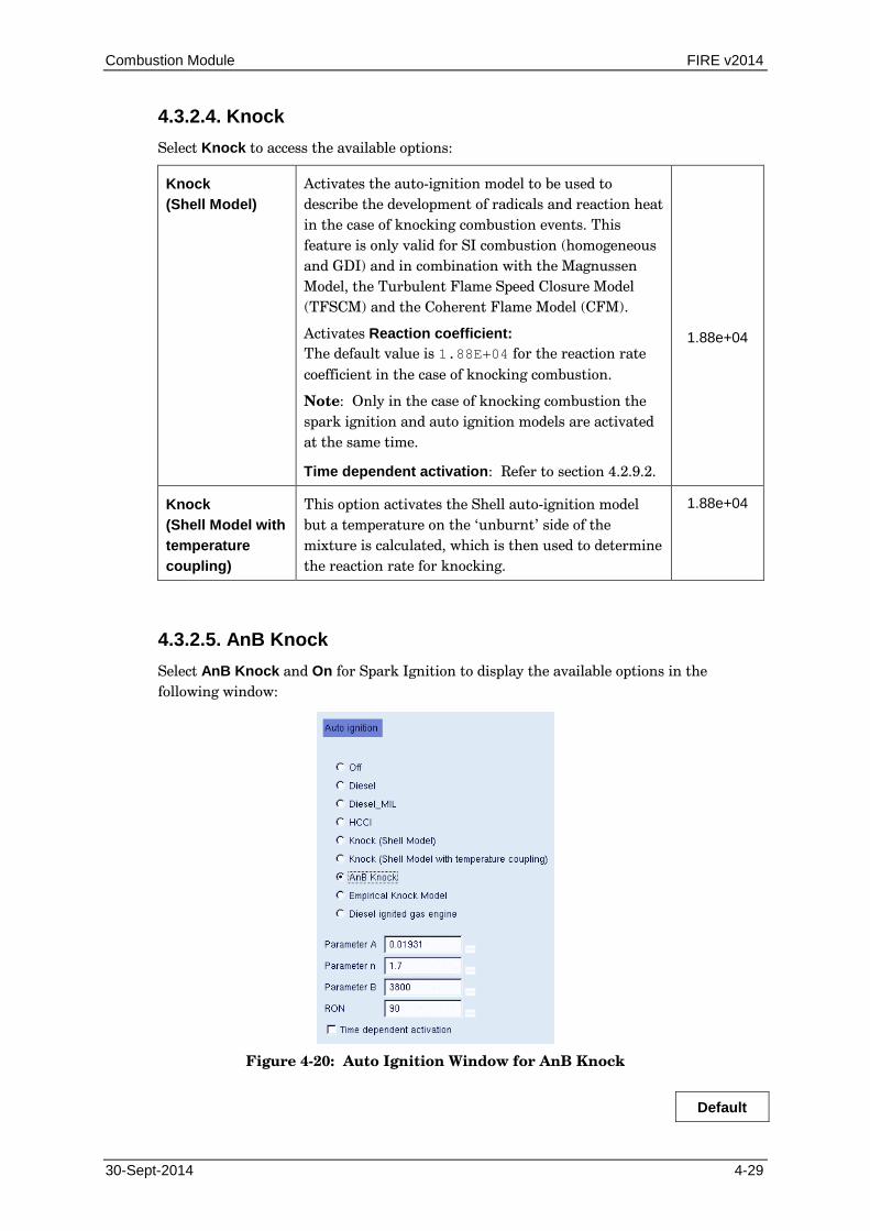
Combustion Module FIRE v2014
30-Sept-2014 4-29
4.3.2.4. Knock Select Knock to access the available options:
Knock (Shell Model)
Activates the auto-ignition model to be used to describe the development of radicals and reaction heat in the case of knocking combustion events. This feature is only valid for SI combustion (homogeneous and GDI) and in combination with the Magnussen Model, the Turbulent Flame Speed Closure Model (TFSCM) and the Coherent Flame Model (CFM).
Activates Reaction coefficient: The default value is 1.88E+04 for the reaction rate coefficient in the case of knocking combustion.
Note: Only in the case of knocking combustion the spark ignition and auto ignition models are activated at the same time.
Time dependent activation: Refer to section 4.2.9.2.
1.88e+04
Knock (Shell Model with temperature coupling)
This option activates the Shell auto-ignition model but a temperature on the ‘unburnt’ side of the mixture is calculated, which is then used to determine the reaction rate for knocking.
1.88e+04
4.3.2.5. AnB Knock Select AnB Knock and On for Spark Ignition to display the available options in the following window:
Figure 4-20: Auto Ignition Window for AnB Knock
Default
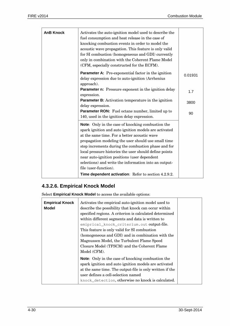
FIRE v2014 Combustion Module
4-30 30-Sept-2014
AnB Knock Activates the auto-ignition model used to describe the fuel consumption and heat release in the case of knocking combustion events in order to model the acoustic wave propagation. This feature is only valid for SI combustion (homogeneous and GDI) currently only in combination with the Coherent Flame Model (CFM, especially constructed for the ECFM).
Parameter A: Pre-exponential factor in the ignition delay expression due to auto-ignition (Arrhenius approach). Parameter n: Pressure exponent in the ignition delay expression. Parameter B: Activation temperature in the ignition delay expression. Parameter RON: Fuel octane number, limited up to 140, used in the ignition delay expression.
0.01931
1.7
3800
90
Note: Only in the case of knocking combustion the spark ignition and auto ignition models are activated at the same time. For a better acoustic wave propagation modeling the user should use small time step increments during the combustion phase and for local pressure histories the user should define points near auto-ignition positions (user dependent selections) and write the information into an output-file (user-function).
Time dependent activation: Refer to section 4.2.9.2.
4.3.2.6. Empirical Knock Model Select Empirical Knock Model to access the available options:
Empirical Knock Model
Activates the empirical auto-ignition model used to describe the possibility that knock can occur within specified regions. A criterion is calculated determined within different segments and data is written to emiprical_knock_criterium.out output-file. This feature is only valid for SI combustion (homogeneous and GDI) and in combination with the Magnussen Model, the Turbulent Flame Speed Closure Model (TFSCM) and the Coherent Flame Model (CFM).
Note: Only in the case of knocking combustion the spark ignition and auto ignition models are activated at the same time. The output-file is only written if the user defines a cell-selection named knock_detection, otherwise no knock is calculated.

Combustion Module FIRE v2014
30-Sept-2014 4-31
4.3.2.7. Diesel Ignited Gas Engine Model The Diesel ignited gas engine model combines homogeneous premixed gas combustion with Diesel ignition. It is possible to use the Eddy Breakup combustion model or the ECFM combustion model for the main burning phase. The auto-ignition model is chosen automatically. Auto-ignition is calculated in regions which are richer than the homogeneous mixture.
Select Diesel ignited gas engine to access the following available options:
Figure 4-21: Window for AnB Knock
Default
Off Active
Automatic This option calculates the mean fuel mass fraction in the whole domain and uses this value as a limit for cells with auto-ignition. Note: This option is recommended.
Manual With this option the user can specify the limiting mass fraction value by hand. Fuel mass fraction limit
0
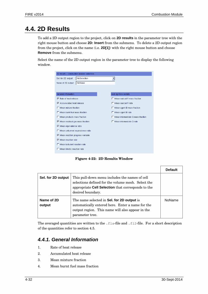
FIRE v2014 Combustion Module
4-32 30-Sept-2014
4.4. 2D Results To add a 2D output region to the project, click on 2D results in the parameter tree with the right mouse button and choose 2D: Insert from the submenu. To delete a 2D output region from the project, click on the name (i.e. 2D[1]) with the right mouse button and choose Remove from the submenu.
Select the name of the 2D output region in the parameter tree to display the following window.
Figure 4-22: 2D Results Window
Default
Sel. for 2D output This pull-down menu includes the names of cell selections defined for the volume mesh. Select the appropriate Cell Selection that corresponds to the desired boundary.
Name of 2D output
The name selected in Sel. for 2D output is automatically entered here. Enter a name for the output region. This name will also appear in the parameter tree.
NoName
The averaged quantities are written to the .fla-file and .fl2-file. For a short description of the quantities refer to section 4.5.
4.4.1. General Information 1. Rate of heat release
2. Accumulated heat release
3. Mean mixture fraction
4. Mean burnt fuel mass fraction

Combustion Module FIRE v2014
30-Sept-2014 4-33
5. Mean products mass fraction
6. Mean residual gas mass fraction
7. Mean equivalence ratio
8. Mean unburned equivalence ratio
9. Mean reaction progress variable
10. Mean reaction rate
11. Mean turbulent reaction rate
12. Mean kinetic reaction rate
4.4.2. Auto Ignition Models 1. Mean radical R mass fraction
2. Mean radical R rate
3. Mean agent B mass fraction
4. Mean agent B rate
5. Mean intermediate Q mass fraction
6. Mean intermediate Q rate
4.5. 3D Results Select 3D results in the parameter tree to display the following window:
Figure 4-23: 3D Results Window

FIRE v2014 Combustion Module
4-34 30-Sept-2014
4.5.1. General Information Default
Mixture fraction The mixture fraction is the burned and unburned fuel mass over the total mass. It is a standard output when the Combustion Module is activated.
tot
b,fuu,fu
mmm
f+
=
Active
Burnt fuel mass fraction
Mass fraction of the burned fuel based on the total mixture mass.
tot
b,fub,fu m
my =
Products mass fraction
The quantity is the mass of combustion products (carbon dioxide and water) over total mass.
tot
OHCOPr m
mmy 22
+=
Residual gas mass fraction
This quantity is only available when exhaust gas return is taken into account during the calculation. It is a standard output when the Combustion Module is activated and illustrates the EGR over the oxidizer mass.
oxid
rg
mm
g =
The oxidizer mass rgairoxid mmm += is the sum of
air mass and residual gas mass.
Active
Equivalence ratio The equivalence ratio is calculated based upon the total mixture mass. The mixture fraction f is based on the total mixture mass.
stFA
f1f
−=φ
This quantity is a standard output when the Combustion Module is activated.
Active
Unburned equivalence ratio
The unburned equivalence ratio is calculated based upon the total mixture mass. The unburned fuel mass fraction yfu is based on the total mixture mass.
stfu
fuu F
Ay1
y
−=φ
Combustion Module FIRE v2014
30-Sept-2014 4-35
Reaction progress variable
The reaction progress variable is available during combustion simulation and represents the mass of combustion products over the theoretical maximum mass of combustion products (bounded between zero and unity).
∞
=Pr,
Pr
yyc
This quantity is a standard output when the Combustion Module is activated.
Active
Reaction rate The quantity is the reaction rate which is the fuel mass fraction depletion rate.
fur⋅ρ
[kg/(m³s)]
Normalized reaction rate
The quantity is the normalized reaction rate which is the fuel mass fraction depletion rate.
( )maxfu
fufu r
rS
⋅ρ⋅ρ
=
Fluctuation intensity
Variance of the reaction progress variable indicates the location of the turbulent reaction zone. The following equation is only valid for the turbulence controlled combustion model.
( )c1cc −=′′
In the PDF model the fluctuation intensity is based on particle properties obtained from the solution of the PDF transport equations.
Active
Flame Contour Flame contour displays the temporal evolution of the flame front like AVL Visiotomo technology. The output is written to the fl3-file within a certain progress variable range from spark onset up to the defined end of the calculation (defined in the GUI).
FIRE v2014 Combustion Module
4-36 30-Sept-2014
Visio knock technology
Defines control volume segments in clockwise direction and calculates AVL Visioknock technology criterion (knock probability) based on the FQ mass fraction normalised by its maximum occurring value within the segments.
Bore A ‘real’ bore has to be defined where 2/3 is used for the determination of the radial limit for the control volume segments.
Cell selection A cell selection (only the combustion chamber is recommended) has to be defined, otherwise no knock probability is calculated (message in fla-file).
Note: This option only makes sense for real engine applications and was mainly constructed for gasoline engines.
0.082 [m]
No Selection
4.5.2. CFM Models Default
Flame surface density
The flame surface density is the local area of the flame per unit of volume. This quantity is only available if the Coherent Flame Model is activated.
Active
[1/m]
Flame surface density rate
This quantity is only available if the Coherent Flame model is activated.
[1/(ms)]
CO/CO2 equilibrium
Dissociation of CO2 to CO for fuel rich mixture when CFM-2A or MCFM are activated, respectively.
4.5.3. Auto Ignition Models Default
Radical R Radical mass fraction R.
Agent B Branching agent mass fraction B.
Intermediate Q Intermediate product mass fraction Q.
Combustion Module FIRE v2014
30-Sept-2014 4-37
4.5.4. Optional Output from Knock Models
4.5.4.1. Knock
Knock_Crit_ Kinetic
The quantity gives the probability of knock occurrence depending on a criterion determined by the mixture fraction f, progress variable c, temperature T and intermediate product mass fraction Q. The higher the value the higher the possibility of knocking. The quantity is a fictitious value.
4.5.4.2. AnB Knock
Precursor_cfm The quantity is the mass fraction of the precursor which grows in time. If this quantity reaches the quantity of unburned fuel mass fraction, then knocking occurs locally resulting in fuel consumption and heat release. This quantity is calculated only in the unburned gas phase since knocking appears only there.