B. Aupoix, D. Arnal Transition and Turbulence Modeling · Transition and Turbulence Modeling Introduction ... tion prediction is of great importance for hypersonic re-entry vehicles

Issue 2 - March 2011 - Transition and Turbulence Modeling AL02-01 1

CFD Plateforms and Coupling

B. Aupoix, D. ArnalH. Bézard, B. Chaouat, F. Chedevergne, S. Deck, V. Gleize, P. Grenard, E. Laroche(Onera)

E-mail: [email protected]

Transition and Turbulence Modeling

Introduction

Fluid motions are fully described by the Navier-Stokes equations which express the conservation of mass, momentum and, if needed, energy and/or chemical species. From a theoretical point of view, solving these equations remains a challenge beyond the present ca-pabilities of mathematicians and is one of the Millennium Problems proposed by the Clay Mathematics Institute. From an engineering point of view, practical flows in aerospace applications are mostly tur-bulent. As turbulence is characterized by a large variety of scales (see e.g. [40]), all these scales must be captured in the flow computation. This is the Direct Numerical Simulation approach (DNS) which is far beyond the capabilities of present and foreseeable computers. Ex-trapolating the progress in computer power and computer sciences, it is expected that the DNS computation of the flow around an airliner in cruise conditions or around a car on a (US) highway could be fea-sible circa 2080 [77]. Therefore, only a simplified vision of the flow can be computed and models are required to represent the part of the physics which cannot be resolved. This holds both for the prediction of the flow instabilities which lead to the transition from the laminar to the turbulent regime and for the fully turbulent regime. Transition and turbulence modeling aspects are detailed below.

Transition modeling

Since the classical experiments performed by Reynolds [65], con-stant interest has been shown in the instability of laminar flows and the transition to turbulence for solving fluid mechanics problems. This interest results from the fact that transition controls important hydro-dynamic quantities such as drag or heat transfer. For instance, the heating rates generated by a turbulent boundary layer may be several times higher than those for a laminar boundary layer; therefore transi-tion prediction is of great importance for hypersonic re-entry vehicles. In the case of commercial transport aircraft at high subsonic speed, the achievement of laminar flow can significantly reduce the drag on the wings and hence the fuel consumption of the aircraft.

When a laminar flow develops along a given body, it is strongly af-fected by various types of disturbances generated by the model itself (roughness, vibrations…) or existing in the free-stream (tur-bulence, noise…). These disturbances are the sources of complex

Although the basic equations of fluid motions have been well known for long, their complete solution in practical applications is beyond the scope of present and fore-

seeable computers. Models are thus required to account for the transition to turbulence mechanisms as well as to represent at least a part of the turbulent motion. This paper aims at giving an overview of the present modeling practices and the models devel-oped or imported by Onera and implemented in the CEDRE and/or elsA solvers.

mechanisms which ultimately lead to turbulence. There are in fact two main paths to turbulence: •Ifthelaminarboundarylayerdevelopsona“perfectlysmooth”wall, in a low free-stream disturbance environment (for instance in flight conditions), transition results from the amplification of unstable waves:thisprocessiscalled“naturaltransition”. • In thepresenceofstrongdisturbances (high free-stream tur-bulence, large roughness elements), these waves are no longer ob-served. In this case, streamwise streaks appear and play a major role inthetransitionprocess;thismechanismhasbeennamed“bypass”by Morkovin [54].

Both aspects will be analyzed successively in the following para-graphs.

Natural transition

General description

To describe the laminar-turbulent transition process in two-dimen-sional (2D) or three-dimensional (3D) boundary layers, it is helpful to distinguish three successive steps, as illustrated in Figure 1. The first step, which takes place close to the leading edge, is the receptiv-ity. Receptivity describes the means by which forced disturbances such as free-stream noise or free-stream turbulence enter the laminar boundary layer and excite its eigenmodes. In the second phase, these eigenmodes take the form of periodic waves, the energy of which is convected in the streamwise direction. Some of them are amplified and will be responsible for transition. Their evolution is well described by the linear stability theory. When the wave amplitude becomes fi-nite, nonlinear interactions occur and lead rapidly to turbulence.

Figure1-“Natural”transitionona2Dflatplate,visualizationinwaterchannel(Werlé, Onera).

Receptivity Linear Non - linear


In 2D flows, the linearly growing waves are referred to as Tollmien-Schlichting (TS) waves. In 3D boundary layer flows, for instance on a swept wing, the mean velocity profile has two components: a stream-wise component u in the external streamline direction, and a cross-flow component w in the direction normal to the previous one. The streamwise velocity profile is unstable in regions of zero or positive pressure gradient (decelerated flows). It generates waves similar to the 2D TS waves, with a wave number direction close to the free-stream direction. The cross-flow velocity profile is highly unstable in negative pressure gradients (accelerated flows). It generates cross-flow (CF) waves with a wave number vector making an angle of 85 to 89º with respect to the free-stream direction.

As it will be explained later, the receptivity process and the nonlinear interactions are different for TS and CF disturbances. In the linear phase, however, the same stability theories are applicable for both types of waves.

Natural transition modeling

In the framework of the classical linear stability theory, the distur-bances are written as:

( )ˆ' ( )expr r y i x z tα β ω= + − (1)

'r is a velocity, pressure or density fluctuation; r is an amplitude function; x and z are the directions normal and parallel to the lead-ing edge, y is the direction normal to the wall. When considering the spatial theory (which is the most relevant for a wide range of bound-ary layer problems), r iiα α α= + is the (complex) wave number in the x direction. β and ω are real and represent the wave num-ber component in the z direction and the frequency. The angle ψdefined as:

tan / rψ β α= (2)

represents the wave number direction, i.e. the direction normal to the wave crests.

Introducing expression (1) into the linearized Navier-Stokes equations and assuming that the mean flow is parallel, leads to a system of ordinary differential equations for the amplitude functions (eigenvalue problem). For the simplest case of a 2D, low speed flow with 0β = , the stability equations can be combined to obtain the well-known Orr-Sommerfeld equation. Depending on the value of ψ , the solutions of the linear stability equations represent either TS or CF waves.

Non linear PSE (Parabolized Stability Equations) can be used in order to model the non linear interactions between waves just before the breakdown to turbulence, see [37]. The disturbances are now ex-pressed as a double series of ( , )n m modes of the form:

ˆ' ( , )exp ( ( ) ) .n m

nm nmn m

r r x y i d m z n tα ξ ξ β ω=+∞ =+∞

=−∞ =−∞

= + − ∑ ∑ ∫ (3)

As for the linear theory, nmα is complex; β and ω are real numbers. Each mode is denoted as ( , )n m ; the integers n and m characterize the frequency and the spanwise wave number, respectively. When these disturbances are introduced into the Navier-Stokes equations, a system of coupled partial differential equations is obtained; this (nearly) parabolic system is solved by a marching procedure in the

x -direction. Any non-linear PSE computation requires a choice of the“mostinteresting”interactionscenariobetweenparticularmodes(“majormodes”)and impositionof initialamplitudes inA for these modes. The numerical results show that the non linear behaviors are different depending on the nature of the dominant instability at transi-tion: in the case of TS waves, resonances between 2D ( 0)β = and oblique modes lead to an sudden increase of the mode amplitudes; in the case of CF waves, a saturation is observed before the breakdown to turbulence.

As far as the receptivity process is concerned, a distinction must be made between TS and CF instabilities: •TSinstabilityisverysensitivetothefree-streamdisturbances(noise or the free-stream turbulence), which are usually quantified by the non-dimensional parameter 6%Tu =. •TheCFwavescoverawidefrequencyrange.Inparticular,zerofrequency waves are highly amplified by the cross-flow mean veloc-ity component w . They take the form of stationary vortices nearly aligned with the external streamlines. At low 6%Tu =, these vortices play the major role in the transition process by creating a steady inflection point on the streamwise velocity profile. It is now recognized that the source of the CF vortices lies in the micron-sized roughness elements (i.e. the surface polishing) at the location where the vortices start to be amplified [61], typically between 1 and 5% chord on a swept wing. It follows that improving the surface polishing of the leading edge decreases the initial amplitude of the vortices and delays transition.

Natural transition prediction

The most popular method for predicting transition is the Ne criterion, developed more than 50 years ago by Smith and Gamberoni [74] and by van Ingen [84], see review in [4]. The so-called N factor is the total growth rate of the most unstable disturbances. For the simplest case of 2D, incompressible flows, it is computed by integrating iα− in the x direction. The procedure becomes more complicated for compressible and/or 3D flows, but the principle remains the same. Transition is assumed to occur for some specified value TN of N ; for instance, TN lies in the range 8-10 on 2D airfoils in low turbulence wind tunnels. The Ne method is based on the linear theory only and does not take the receptivity and the non linear mechanisms into ac-count explicitly.

As the use of the Ne method is often time consuming, the develop-ment of simplified methods is of unquestionable practical interest. The simplest solution is to apply analytical criteria expressing rela-tionships between boundary layer integral parameters at the transition point, see for instance [53], [35], [3]. The latter criteria have been implemented in the elsA code. Another possibility is to use simplified stabilitymethods(theso-called“databasemethods”),thecomplexityof which is intermediate between analytical criteria and exact stability computations [59].

The above methods, however, are not well adapted to massively par-allel RANS computations because they use non-local quantities such as momentum thickness or shape factor. To avoid these difficulties, Menter [52] proposed a purely local transition model which consists of two transport equations for the intermittency function and for a pseudo-momentum thickness Reynolds number, coupled with a SST

kω− turbulence model. At Onera, this model has been implemented in the elsA code. Once calibrated by comparison with experimental


data or stability results, it gives satisfactory results for 2D flows, see [23]. It does not include the cross-flow instability.

At first sight, the non linear PSE could be considered as the most rigorous tool for transition prediction, because they describe both the linear and the non linear developments of the unstable waves. However, it is important to keep in mind that the abscissa corre-sponding to the resonance (for TS waves) or to the mode saturation (for CF waves) depends on the initial amplitude inA imposed on the major modes. Increasing inA leads to an upstream movement of this abscissa and of the numerical breakdown location. In other words, the choice of the N factor, which constitutes the major difficulty of the linear Ne method, is now replaced by the choice of inA . Therefore the non linear PSEs cannot yet be considered as mature enough for practical transition prediction. A measure of the receptivity is needed.

Bypass Transition

General description

In many practical situations, laminar-turbulent transition occurs at lower Reynolds numbers than those predicted by the classical lin-ear stability theory. This suggests that another transition mechanism mayexist.Thisprocess,called“transientgrowth”,resultsfromthenon-normality of the eigenfunctions (solutions of the linear stability equations): if two eigenfunctions are not orthogonal, the perturbation energy of their sum can increase even if both of them are damped. The physics of the transient growth is the following. A longitudinal vortex superimposed to the boundary layer shear stress pushes up low speed particles from the wall to the top of the shear layer, and pulls down high speed particles toward the wall, leading to a span-wise alternation of low and high speed streamwise structures called streaks. This phenomenonwascalled “lift-up”byLandahl [43]. Inother words, as soon as longitudinal vortices are present in a laminar boundary layer, streaks are likely to appear rapidly downstream. An early laminar-turbulent transition can be triggered if the energy of the streaksgrowssignificantly; this is the“bypass” transitionprocess,meaning that the classical process driven by the TS or CF waves has been short-circuited.

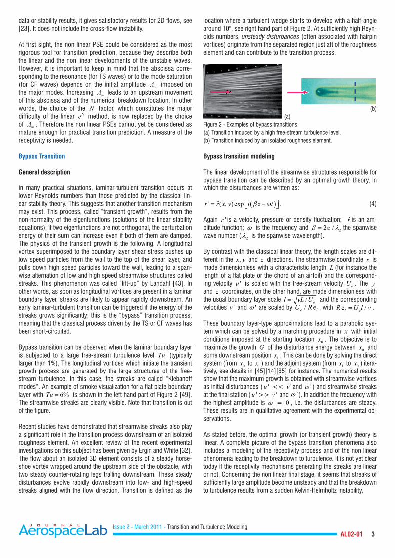
Bypass transition can be observed when the laminar boundary layer is subjected to a large free-stream turbulence level Tu (typically larger than 1%). The longitudinal vortices which initiate the transient growth process are generated by the large structures of the free-stream turbulence. In this case, the streaks are called “Klebanoffmodes”.Anexampleofsmokevisualizationforaflatplateboundarylayer with 6%Tu = is shown in the left hand part of Figure 2 [49]. The streamwise streaks are clearly visible. Note that transition is out of the figure.

Recent studies have demonstrated that streamwise streaks also play a significant role in the transition process downstream of an isolated roughness element. An excellent review of the recent experimental investigations on this subject has been given by Ergin and White [32]. The flow about an isolated 3D element consists of a steady horse-shoe vortex wrapped around the upstream side of the obstacle, with two steady counter-rotating legs trailing downstream. These steady disturbances evolve rapidly downstream into low- and high-speed streaks aligned with the flow direction. Transition is defined as the

location where a turbulent wedge starts to develop with a half-angle around 10°, see right hand part of Figure 2. At sufficiently high Reyn-olds numbers, unsteady disturbances (often associated with hairpin vortices) originate from the separated region just aft of the roughness element and can contribute to the transition process.

(b) (a)Figure 2 - Examples of bypass transitions.(a) Transition induced by a high free-stream turbulence level.(b) Transition induced by an isolated roughness element.

Bypass transition modeling

The linear development of the streamwise structures responsible for bypass transition can be described by an optimal growth theory, in which the disturbances are written as:

( )ˆ' ( , ) exp .r r x y i z tβ ω= − (4)

Again 'r is a velocity, pressure or density fluctuation; r is an am-plitude function; ω is the frequency and 2 / Zβ π λ= the spanwise wave number ( Zλ is the spanwise wavelength).

By contrast with the classical linear theory, the length scales are dif-ferent in the ,x y and z directions. The streamwise coordinate x is made dimensionless with a characteristic length L (for instance the length of a flat plate or the chord of an airfoil) and the correspond-ing velocity 'u is scaled with the free-stream velocity eU . The y and z coordinates, on the other hand, are made dimensionless with the usual boundary layer scale / el vL U= and the corresponding velocities 'v and 'ω are scaled by / ee lU R , with e /l eR U l v= .

These boundary layer-type approximations lead to a parabolic sys-tem which can be solved by a marching procedure in x with initial conditions imposed at the starting location 0x . The objective is to maximize the growth G of the disturbance energy between 0x and some downstream position 1x . This can be done by solving the direct system (from 0x to 1x ) and the adjoint system (from 1x to 0x ) itera-tively, see details in [45][14][85] for instance. The numerical results show that the maximum growth is obtained with streamwise vortices as initial disturbances ( 'u << 'v and 'ω ) and streamwise streaks at the final station ( 'u >> 'v and 'ω ). In addition the frequency with the highest amplitude is ω = 0 , i.e. the disturbances are steady. These results are in qualitative agreement with the experimental ob-servations.

As stated before, the optimal growth (or transient growth) theory is linear. A complete picture of the bypass transition phenomena also includes a modeling of the receptivity process and of the non linear phenomena leading to the breakdown to turbulence. It is not yet clear today if the receptivity mechanisms generating the streaks are linear or not. Concerning the non linear final stage, it seems that streaks of sufficiently large amplitude become unsteady and that the breakdown toturbulenceresultsfromasuddenKelvin-Helmholtzinstability.


Bypass transition prediction

Many empirical criteria have been developed for many years in order to predict the occurrence of bypass transitions. For instance, the ef-fect of high free-stream turbulence levels is taken into account by the well-known correlation proposed by Abu Ghannam and Shaw [1]. Concerning the problem of boundary layer tripping by large, isolated 3D roughness elements of height k , a relevant parameter is a char-acteristic Reynolds number Rk defined as:

k

k

U kRk

ν= (5)

kU and kv denote the mean velocity and the kinematic viscosity at the altitude y k= . These values are computed in the undisturbed flow. Von Doenhoff and Braslow [87] developed an empirical correlation between the critical value of Rk (denoted as critRk ) which triggers transition and the ratio /d k , where d is a measure of the spanwise or chordwise extent of the protuberance (for circular cylinders normal to the wall, d is the diameter). critRk is of the order of 500-600 for

/ 1d k = and 200-250 for / 10d k = . Systematic applications of this criterion showed that it remains valid for a wide range of applications, in 2D and 3D flows, from subsonic to supersonic flows.

The transition model proposed by Menter et al. [52] can also predict transition in the presence of large values of Tu. Examples of applica-tions for turbo-machinery problems using the RANS code elsA can be found in [11].

Quite recently, attempts have been made to use the transient growth theory in order to quantify or to predict the effects of roughness on transition. Following the work of Luchini [45], Vermeersch [85][86] developed a system of parabolic, linear transport equations for the streamwise velocity and temperature fluctuations of the streamwise streaks. To close the system, the vertical velocity fluctuation 'v is modeled by an analytical relationship. Transition is assumed to occur when the ratio between the shear stress generated by the streaks to the viscous stress reaches some predefined critical value. This model was successfully applied to bypass transition problems, both in the case of large free-stream turbulence levels and in the case of bound-ary layer tripping by large roughness elements. In the latter case, it was possible to determine a theoretical curve for critRk as a function of /d k . This curve was in good agreement with the von Doenhoff and Braslow criterion mentioned above. This confirms that the tran-sient growth theory contains (at least a part of) the physics of the boundary layer tripping mechanisms.

Outlooks

After more than fifty years, the Ne method remains the most widely usedmethodtoestimatethe“natural”transitionlocation,althoughitsdeficiencies are well identified: the receptivity mechanisms are not accounted for explicitly and the nonlinear phase is replaced by a con-tinuous linear amplification up to the onset of transition. The nonlinear PSE equations, on the other hand, are now a classical research tool. Although they cannot be used for systematic practical applications, they are a help in understanding the basic phenomena leading to tran-sition. As much information has been collected during the last ten or fifteen years on receptivity, a rather complete but partly empirical modelingof“natural”transitionisnowavailable.

The state-of-the-art for the modeling of bypass transition is not so advanced. Most of the practical prediction methods used today are based on simple criteria, which ignore the complicated physics of the phenomena. Recent investigations have shown that the linear transient growth theory appears to be an efficient tool for the under-standing and the modeling of these phenomena. The validity of this approach needs to be validated in complex situations, in particular for 3D and/or compressible flows. In addition, the picture of the receptiv-ity and non linear mechanisms has to be completed.

Turbulence modeling

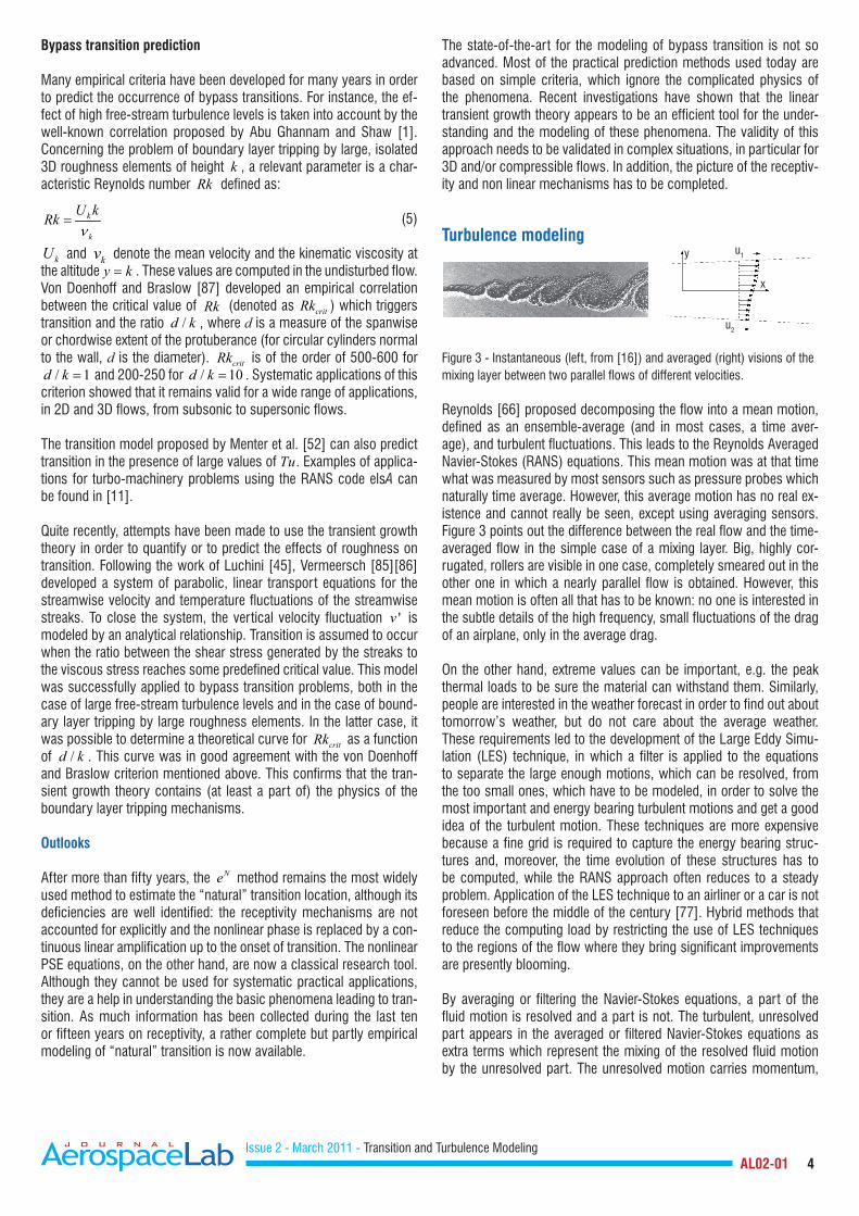
Figure 3 - Instantaneous (left, from [16]) and averaged (right) visions of the mixing layer between two parallel flows of different velocities.

Reynolds [66] proposed decomposing the flow into a mean motion, defined as an ensemble-average (and in most cases, a time aver-age), and turbulent fluctuations. This leads to the Reynolds Averaged Navier-Stokes (RANS) equations. This mean motion was at that time what was measured by most sensors such as pressure probes which naturally time average. However, this average motion has no real ex-istence and cannot really be seen, except using averaging sensors. Figure 3 points out the difference between the real flow and the time-averaged flow in the simple case of a mixing layer. Big, highly cor-rugated, rollers are visible in one case, completely smeared out in the other one in which a nearly parallel flow is obtained. However, this mean motion is often all that has to be known: no one is interested in the subtle details of the high frequency, small fluctuations of the drag of an airplane, only in the average drag.

On the other hand, extreme values can be important, e.g. the peak thermal loads to be sure the material can withstand them. Similarly, people are interested in the weather forecast in order to find out about tomorrow’s weather, but do not care about the average weather. These requirements led to the development of the Large Eddy Simu-lation (LES) technique, in which a filter is applied to the equations to separate the large enough motions, which can be resolved, from the too small ones, which have to be modeled, in order to solve the most important and energy bearing turbulent motions and get a good idea of the turbulent motion. These techniques are more expensive because a fine grid is required to capture the energy bearing struc-tures and, moreover, the time evolution of these structures has to be computed, while the RANS approach often reduces to a steady problem. Application of the LES technique to an airliner or a car is not foreseen before the middle of the century [77]. Hybrid methods that reduce the computing load by restricting the use of LES techniques to the regions of the flow where they bring significant improvements are presently blooming.

By averaging or filtering the Navier-Stokes equations, a part of the fluid motion is resolved and a part is not. The turbulent, unresolved part appears in the averaged or filtered Navier-Stokes equations as extra terms which represent the mixing of the resolved fluid motion by the unresolved part. The unresolved motion carries momentum,

u1

u2

x

y


energy or chemical species within the resolved part. The averaging or filtering thus introduces turbulent stresses and heat or species fluxes which have to be modeled. There are six independent components for the turbulent stress tensor and three for the heat or species flux vectors. The system of equations is now unclosed; as there are more unknowns than equations, models are required.

RANS approach

Present status

As pointed out above, turbulent, or Reynolds, stresses and turbulent heat or species fluxes appear in the Reynolds Averaged Navier-Stokes equations. Transport equations for these quantities can be derived from the Navier-Stokes equations. However, the information lost in the averaging process cannot be retrieved, so that these transport equations involve new terms, for which transport equations could be derived, and so on ad infinitum… Modeling is thus required.

In the RANS approach, the modeling of the turbulent stresses and heat or species fluxes heavily relies upon the assumption that the turbulent motion is close to an equilibrium state. Although there is a large range of turbulent scales, with this assumption, the turbulent motion can be characterized by the knowledge of the large, energy bearing scales, the energy distribution in the smaller scales being imposed from the large scales. Therefore, most models only characterize turbulence by two quantities: a turbulent velocity scale and a turbulent length (or equivalently time) scale. The turbulent velocity scale is often deduced from the turbulent kinetic energy, usually labeled k , the transport equation of which is easily derived from the Navier-Stokes equations and the modeling of which is relatively simple.

RANS turbulence models can be sorted into three main groups:In the first group, Eddy Viscosity Models (EVM) assume an analogy between the mixing of the averaged flow by the turbulent motion and the transport by the Brownian motion of particles within gases to express the turbulent stresses and heat or species fluxes in a way similar to the viscous stresses and heat or species fluxes. They thus introduce an eddy viscosity, thermal conductivity or diffusivity which, unlike its laminar counterpart, is not a property of the fluid but of the flow motion. From dimensional analysis, they are proportional to the product of the turbulent velocity and length scales. This ap-proach is not fully justified: there is no scale separation between the mean and turbulent motions as there is a scale separation between the gas motion and the Brownian motion. Nevertheless, such mod-els are widely used in the industry as they can give fair predictions of simple, sheared flows, such as boundary layers, wakes, mixing layers… which are of large practical importance. The most popular eddy viscosity models were k ε− models (e.g. [44]) where ε is the turbulent kinetic dissipation rate, i.e. the rate at which turbulent kinetic energy is transformed into heat, and gives a turbulence length scale (see, e.g. [40]). These k ε− models usually fail to predict boundary layer separation and hence, e.g. ,overestimate the maximum airfoil lift or the compressor performances. They are superseded by the Spalart and Allmaras model [75] and by k ω− models, mainly the Shear Stress Transfert (SST) model [50], which give improved predictions and are now aeronautic industry workhorses. Again mimicking fluid properties, the thermal conductivity and diffusivity are generally de-duced from the eddy viscosity by respectively assuming constant turbulent Prandtl and Schmidt numbers. Although this is nearly the only approach used, it is not fully justified. The standard value for the

turbulent Prandtl number (0.9) holds in the main part of the boundary layer, but not very close to the wall, nor in free shear flows.

The second group solves the crudeness of the eddy viscosity assump-tion which cannot represent correctly all of the components of the turbulent stress tensor and of the heat or species flux vectors. More complex relationships, similar to the ones used in rheology, or derived from tensor representation theorems, can be used to express the tur-bulent stresses and heat or species fluxes in terms of the turbulence length and velocity scales and of the mean flow gradients. These mod-els are named Non-Linear Eddy Viscosity Models (NLEVM) or Explicit Algebraic Reynolds Stress Models (EARSM) according to the way they are derived. Non-linear representations can also be used to model the heat or species flux vector. These non-linear models provide fair repre-sentations of all of the components of the turbulent stress tensor and of the heat or species flux vector and hence better predictions of more complex flows than simple sheared flows, e.g. they can capture some rotation and curvature effects, as shown in Figure 4.

All the above models link the turbulent stresses and heat or species flux to local velocity, temperature and species gradients. However, turbulence does not adjust instantaneously to the mean flow. This leads to the third group of models, solving the transport equations for the turbulent stresses (and for the turbulent heat or species flux) to capture the turbulence memory and non-equilibrium effects. This re-quires a larger effort as there are six independent components to the turbulent stress tensor and moreover information about the turbulent length scale is still required. The use of Reynolds stress transport equations is an old practice at the academic level (see, e.g. [55]), mainly in pressure-based codes for incompressible flows. Those models seem particularly appropriate to describe flows characterized by separation, rotation and strong curvature effects such as encoun-tered in turbo-machinery [38]. Their introduction in industrial codes, solving averaged Navier-Stokes equations for compressible flows, is a breakthrough of the European research project FLOMANIA [36]. When the thermal problem is considered, three transport equations for the heat flux vector components are to be added, and generally two more transport equations for characteristic scales for the turbulent thermal field, which leads to twelve transport equations. Transport models for the turbulent heat or species fluxes are thus still at the research level.

0.1

0.8

0.6

0.4

0.2

0.0

0.0 0.25 0.5 0.75 1.0

k ε−EARSM

Exp. Imao

0 /U RΩ

/r R

Figure 4 - Mean azimuthal velocity profiles in a rotating pipe: the k ε− eddy viscosity model cannot capture the rotation effect upon the turbulent motion and predicts a solid body rotation while the EARSM does and gives fair predictions.


Some Onera achievements

As pointed out by the Reno workshop organized by NASA to define the needs in turbulence modeling [67], the prediction of boundary layer separation, which e.g. governs the maximum lift or compressor performance predictions, has been a big challenge for a long time. The idea of imposing mathematical constraints to turbulence models was proposed by Cousteix et al. [24] and extended by Catris and Aupoix [18] to correctly capture the physics of boundary layers close to separation. This finally led to the derivation of the k kL− model by Bézard and Daris [13]. This model has been derived in an eddy vis-cosity form and in an EARSM form and is one of the models currently used by Dassault Aviation.

Extra transport equations for the thermal scales can be added to get rid of the constant turbulent Prandtl number hypothesis. The above mentioned k kL− model has been complemented with its thermal counterpart as a four equations k kL k k Lθ θ θ− − − model. This set of scale equations can be coupled with a simple eddy viscosity/thermal conductivity formulation, thus producing physical variations of the turbulent Prandtl number while keeping the simplicity and robustness of classical two-equation models [12], or with more complex explicit algebraic expressions for improving the Reynolds stress tensor and the heat flux vector representation [31].

Another important problem of turbulent flows comes from the effect of strong deviations from equilibrium caused, for instance, by rapid variations in the mean flow. This aspect is mirrored through the well-known weaknesses of the usual modeled dissipation rate equation. Such complex situations rule out the underlying hypothesis of spec-tral equilibrium that is implicitly assumed in classical RANS models. For dealing with non-equilibrium situations, new models using several length scales and called multiscale models have been introduced [71] and further developed by split spectrum schemes devised to mimic in an approximate way the change of the spectrum shape. The mul-tiscale concept takes into account some spectral information while staying within the useful framework of the RANS modeling. From a practical point of view, many levels of closure can be considered, but in practice, two spectral slices will be sufficient to describe the effects of non equilibrium distributions. In this context, four-equation multiscale turbulence models based on a split spectrum energy-flux scheme and energy frequency scheme [Masson, 1996] were devel-oped and successfully applied on several basic and more complex 2D and 3D non-equilibrium flows such as shock-boundary layer interac-tion, transonic channels and an airfoil in stall conditions.

Compressibility can strongly affect the turbulence dynamics. In most aeronautic applications, the turbulent motion remains nearly incom-pressible, so that the key effect is linked to the mean density varia-tions. Turbulence models are developed for incompressible flows and usually straightforwardly applied to compressible flows. The analysis of scalings in a compressible boundary layer gave the hint that the current practice is not correct and led to the derivation of a general rule to extend any turbulence model to correctly account for density gradients within a boundary layer flow [17].

High speed mixing layers, which are encountered e.g. in scramjets, are among the rare examples of aeronautic flows where the turbulent motion can exhibit a compressible character. The sonic eddy concept [15] states that any turbulent structure must be such that information can circulate within it, i.e. the velocity difference between two points

must always be smaller than the speed of sound. This yields a limit on the turbulence length scale, which was first validated and then used to extend in a general way any turbulence model to capture this compressibility effect [6].

As the refraction index is linked to the density, density fluctuations within the flow affect the optical properties of the flow. This has led to the development of aero-optical models for deducing the image blurring from a RANS computation. This requires modeling of both the density fluctuation variance and the way density fluctuations are cor-related along the optical path. Models have been derived for bound-ary layer and mixing layer flows, and validated with respect to LES simulations [83], [7].

Onera has developed a large expertise in flows over rough surfaces, for a wide range of applications such as turbo-machinery or solid pro-pellant rocket nozzles. The standard way to account for wall rough-nessin industrialcodesisthe“equivalentsandgrain”approach, inwhich the turbulence model is altered in the wall region to reproduce the drag and heat transfer increases. A general technique to extend any turbulence model to account for wall roughness has been devel-oped and applied to several turbulence models [5], [8]. This tech-nique has also been adapted to account for riblets, small grooves on the wall surfaces like on shark skin, which can equally well lead to a reduction or increase in drag [10].

Of course, most of these models or model improvements are imple-mented in CEDRE and elsA.

Some outlooks

The prediction of the separation point is now fairly well understood. However, the model behavior in the separated region, especially close to the separation and reattachment points, is still an issue as models usually underestimate turbulence in this region. This is one of the topics addressed by the European ATAAC project (http://cfd.mace.manchester.ac.uk/twiki/bin/view/ATAAC/WebHome) in which Onera is involved.

The present industrial trend is to move from eddy viscosity models towards non-linear models and models with transport equations for the Reynolds stresses. A first Reynolds stress model is implemented in elsA, others will soon be, and the improvement of the Reynolds stress transport models is one of the present activities of Onera.

It has been shown that classical Reynolds stress transport models, which only use information about the Reynolds stress and the turbu-lence length scale, are unable to reproduce some flow cases. This is blamed upon the lack of information about the underlying turbu-lence spatial structures. Cooperation with the University of Cyprus has started on models which account for turbulence structures [9].

For thermal applications, there is a trend to get rid of the constant turbulent Prandtl number assumption, and to move to non-linear rep-resentations of the turbulent heat flux vector through explicit algebraic expressions. Onera plans to develop, implement and test improved thermal models, with particular attention to hot exhaust jet applica-tions. The next step of directly transporting the heat flux components is promising but needs further developments before being used in-dustrially.


Approaches to resolving turbulence

Direct Numerical Simulations

New industrial needs in aerodynamics include transient dynamics of separated flows as well as the control of noise so the simulation of unsteady turbulent flows is now required. Consequently, a steady RANS solution would not be what the engineer needs in these kinds of applications. But, remembering that one of the salient features of tur-bulent flows is their multiscale character, Direct Numerical Simulation can explicitly simulate all of the active scales present in a turbulent flow, since the governing equations are discretized directly and solved numerically. The total number of nodes of such a “modeling free”simulation may scale as 3(Re )LO where ReL denotes the Reynolds number based on the integral length scale. If solid walls are present, the near wall structures need to be resolved leading to an even stron-ger dependence on the Reynolds number. Practical turbulent flows encountered in aeronautics exhibit such a wide range of excited length and time scales (shock waves, boundary and free shear layers,…) at high Reynolds number 5 8( 10 10 )≈ − that DNS becomes inappropri-ate due to prohibitive cost. In other words, DNS remains an efficient research tool which gives significant insights into turbulence physics but will not be used as a predictive tool for design purposes for at least several decades. This is one of the reason why modeling is necessary prior to solving the Navier Stokes equations.

Large Eddy Simulations

The Large Eddy Simulation approach relies on a decomposition of the field between the large and the small scales of the flow. This approach seeks to directly calculate the largest ones (responsible for turbulence production) while modeling the effects of the smaller-scale eddies. The primary obstacle to practical use of LES on industrial flows which involve wall boundary layers at high Reynolds number remains com-puting power resources. Indeed, the scales of motion responsible for turbulence production impose severe demands on the grid. In [77], it is proposed that LES of wall turbulence should be considered as a quasi-DNS (QDNS) since the requested resolution for capturing the near wall layer is roughly ten times less expensive than for DNS. The accuracy of DNS/LES for wall-bounded flows has been recently as-sessed at Onera in various applications including transitional flows [46], [63] and flow control applications [25], [57].

Hybrid methods

Hybrid RANS/LES was invented to alleviate the LES resolution con-straints in the near-wall regions. Basically, the objective is to combine the fine-tuned RANS modeling in the attached boundary layers with the accuracy of LES in the separated regions. Hybrid methods can be categorized into two major classes corresponding respectively to "global" and "zonal" hybrid methods (or "weak" and "strong" RANS/LES coupling methods, see Figure 5). We should point out to the read-er that some flow situations are characterized by a scale separation between the unsteadiness of the mean field and turbulence. This situ-ation arises when the boundary condition imposes flow unsteadiness (like the flow around a helicopter blade). Subsequently, unsteady sta-tistical approaches like URANS (Unsteady Reynolds Averaged Navier Stokes) might be used. However, many cases such as a landing gear do not have this scale separation.

Figure 5 - Classification of unsteady approaches according to levels of mod-eling and readiness (adapted from Sagaut, Deck and Terracol [68]).

Among hybrid RANS/LES methods, the approach that has probably drawn most attention in the recent time frame is the Detached Eddy Simulation (DES97) which was proposed by Spalart et al. [76] (see also [79]). The idea is to simulate the attached boundary layer in RANS mode whereas the separated flow should be ideally simulated in LES mode. The methods in which the attached boundary layer is modeled in RANS mode can be considered as weak RANS/LES cou-pling methods since there is no mechanism to transfer the modeled turbulence energy into resolved turbulence energy. These methods introduce a "grey-area" in which the solution in neither pure RANS nor pure LES since the switch from RANS to LES does not imply an instantaneous change in the resolution level. In practice, the eddy viscosity remains continuous across the RANS/LES interface but the rapid decrease of the level of RANS eddy viscosity enables the development of strong instabilities. This family of techniques is well adapted for simulating massively separated flows characterized by a large scale unsteadiness dominating the time-averaged solution (see [68] for further discussion). Two weaknesses in the use of hybrid methods for technical flows have been identified traditionally. The first one concerns a possible delay in the formation of instabilities in mixing layers due to the advection of the upstream RANS eddy viscosity. The second one deals with the treatment of the "grey-area", where the model switches from RANS to LES, and where the veloc-ity fluctuations, the "LES-content", are expected not to be sufficiently developed to compensate for the loss of modeled turbulent stresses ("Model-Stress Depletion" (MSD)). This can lead to unphysical out-comes, like an underestimation of the skin friction which, at worst, canleadtoartificialseparationdenotedas“GridInducedSeparation”(GIS). In order to get rid of this latter drawback, Spalart et al. [78] proposed a modification of the model length scale presented as a Delayed Detached Eddy Simulation (DDES) to delay the switch into the LES mode and to prevent "Model-Stress Depletion". This method, implemented in both CEDRE and elsA solvers has been successfully used to simulate the buzz in a supersonic inlet [82], side-loads in an over-expanded nozzle flow [30] as well as the reactive flow over a backward facing step [70].

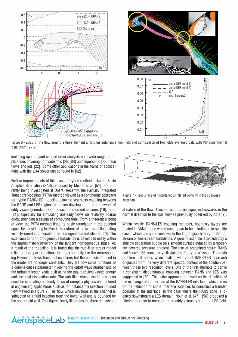
In a different spirit, Deck [26], [27] proposed a Zonal Detached Eddy Simulation (ZDES) approach, in which RANS and DES domains are selected individually. The motivation is to be fully safe from MSD and GIS and to clarify the role of each region. An example of application of this method on a high-lift device is provided in Figure 6. Besides this case, ZDES has been thoroughly validated with experimental data

DNS

LES

Zonal methods«strong RANS/LES coupling»

Global hybrid methods«weak RANS/LES coupling»

Unsteady Statistical Approaches

«PHYSICAL»«NUMERICAL»

Effet of gridrefinement

PHYSICS

Resolved

Modeled

What we need

What wehave

Com

puta

tiona

l cos

t inc

reas

ing

Hybr

id R

ANS/

LES

met

hods


including spectral and second order analysis on a wide range of ap-plications covering both subsonic [28][88] and supersonic [73] base flows and jets [22]. Some other applications in the frame of applica-tions with the elsA solver can be found in [62].

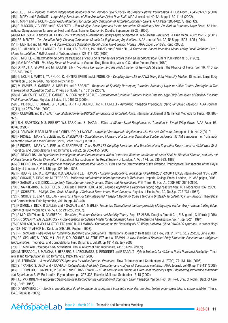
Further improvements of this class of hybrid methods, like the Scale Adaptive Simulation (SAS) proposed by Menter et al. [51], are cur-rently being investigated at Onera. Recently, the Partially Integrated Transport Modeling (PITM) method viewed as a continuous approach for hybrid RANS/LES modeling allowing seamless coupling between the RANS and LES regions has been developed in the framework of eddy viscosity models [72] and second moment closures [19], [20], [21], especially for simulating unsteady flows on relatively coarse grids, providing a saving of computing time. From a theoretical point of view, the PITM method finds its basic foundation in the spectral space by considering the Fourier transform of the two-point fluctuating velocity correlation equations in homogeneous turbulence [20]. The extension to non-homogeneous turbulence is developed easily within the approximate framework of the tangent homogeneous space. As a result of the modeling, it is found that the sub-filter stress model relies on transport equations that look formally like the correspond-ing Reynolds stress transport equations but the coefficients used in the model are no longer constants. They are now some functions of a dimensionless parameter involving the cutoff wave number and of the turbulent length scale built using the total turbulent kinetic energy and the total dissipation rate. The sub-filter stress model has been used for simulating unsteady flows of complex physics encountered in engineering applications such as for instance the injection induced flow viewed in Figure 7. The flow which develops in the channel is subjected to a fluid injection from the lower wall and is bounded by the upper rigid wall. This figure clearly illustrates the three dimension-

al nature of the flow. These structures are squeezed upwards in the normal direction to the axial flow as previously observed by Apte [2].

Within "weak" RANS/LES coupling methods, boundary layers are treated in RANS mode which can appear to be a limitation in specific cases which are quite sensitive to the Lagrangian history of the up-stream or free-stream turbulence. A generic example is provided by a shallow separation bubble on a smooth surface induced by a moder-ate adverse pressure gradient. The use of predefined "pure" RANS and "pure" LES zones may alleviate this "grey-area" issue. The main problem that arises when dealing with zonal RANS/LES approach originates from the very different spectral content of the solution be-tween these two resolution levels. One of the first attempts to derive a consistent discontinuous coupling between RANS and LES was suggested in [60]. This latter approach is based on the definition of the exchange of information at the RANS/LES interface, which relies on the definition of some interface variables to construct a transfer operator at the interface. In the case where the RANS zone is lo-cated downstream a LES domain, Nolin et al. [47], [56] proposed a filtering process to reconstruct an eddy viscosity from the LES field.

0.6

0.4

0.2

0

-0.2

-0.4

-0.6

-0.8

2D - URANS

3D - URANS

3D - DES

0 0.5 1 1.5

xc

yc

Figure 7 - Isosurface of instantaneous filtered vorticity in the spanwise direction.

Exp. EUROPIV2: dashed lineHybrid RANS/LES: solid line

Figure 6 - ZDES of the flow around a three-element airfoil. Instantaneous flow field and comparison of Reynolds averaged data with PIV experimental data (from [27]).

d/czonal DES (grid 1)zonal DES (grid 2)S.Aexp. Europiv2

0.08

0.07

0.06

0.05

0.04

0.03

0.02

0.01

0 0.5 1 1.5

U/U


tions for spatially developing turbulent flows remains one of the chal-lenges that must be addressed prior to the application of LES and hy-brid RANS/LES to industrial flows [69]. Several techniques including mapping/recycling methods or synthetic turbulence methods have been developed (see [41] for a review). Some recent applications at Onera on synthetic methods can be found in [81], [58], [29], [33] in the frame respectively of NLDE, LES and ZDES.

Some outlooks

In the frame of hybrid RANS/LES methods, it can be concluded that current approaches can handle accurately massively separated flows at high Reynolds numbers for which the location of separation is more or less triggered by the geometry. Conversely, as discussed by Sagaut and Deck [69], one of the next foreseen challenges will be firstly to simulate accurately shallow separation and more generally pressure-gradient-driven separation issues. Such simulations imply the ability to capture accurately the boundary layer dynamics at high Reynolds number and eventually transition. So far, most LES (in a wall-turbulence resolved sense) have concerned low Reynolds num-ber and two-dimensional configurations (the span being considered as a homogeneous direction). The next foreseeable challenge will then concern the ability to handle accurately geometrically complex configurations with validated numerical tools at relevant Reynolds numbers.

Conclusion

This article has given an overview of the variety of modeling ap-proaches presently investigated and developed at Onera, ranging from the solution of averaged equations (eN approach for transition and RANS approach for turbulent flows) to the model-free solution of the Navier-Stokes equations, through LES and hybrid approaches. Each class of approach has its strengths and deficiencies, in terms of ability to reproduce the physics as well as of computing cost, the more accurate approaches being the more expensive, or even un-affordable. Short and medium term outlooks have been discussed for each type of models. Although industry can currently only deal with averaged approaches for everyday design, developing expertise on each modeling level ensures that Onera is able to respond to all of today’s and tomorrow’s industrial demands and to improve each modeling level from the knowledge gained from other levels. The large majority of models presented here are available in the CEDRE and/or elsA solvers.

Author names appear in alphabetic order.

The zonal RANS/LES coupling method has been successfully used to simulate the transitional and separated flow around an airfoil near stall [64] (Figure 8). In addition, we should also mention the NLDE (Non-Linear Disturbance Equations) approach extended to the case of a RANS/LES decomposition [42]. Within this perturbation approach, the LES field is broken down as the sum of a mean field (RANS) and a turbulent fluctuation which is computed using modified filtered Navier-Stokes equations (see [80] for a successful application of this method in aeroacoustics).

The case where the LES domain is located downstream from a RANS domain is probably the more difficult to deal with since appropriate inflow conditions need to be specified. The generation of inlet condi-

"Hairpins"

2D modes

Spanwise deformation

3D structures in the reattachment zone

Figure 8 - Transitional and separated flow around an OA209 airfoil near stall. a) Pressure fluctuation contours p’=-2,1.10-3 Pa b) Streamwise velocity fluctuations u’

References

[1] B. ABU-GHANNAM and R. SHAW - Natural Transition of Boundary Layers - The Effects of Turbulence,Pressure Gradient and Flow History. Journal of Mechani-cal Engineering Sciences, 22(5): 213-228 (1980).[2] S.A. APTE and V. YANG - A Large Eddy-Simulation Study of Transition and Flow Instability in a Porous-Walled Chamber with Mass Injection. Journal of Fluid Mechanics, vol. 477, pp. 215-225 (2003).[3] D. ARNAL, M. HABIBALLAH and C. COUSTOLS - Laminar Instability Theory and Transition Criteria in Two- and Three-Dimensional Flows. La Recherche Aérospatiale 1984-2 (1984).[4] D. ARNAL - Practical Transition Prediction Methods: Subsonic and Transonic Flows. VKI Lectures Series Advances in Laminar-Turbulent Transi-tion Modeling (2008).[5] B. AUPOIX and P.R. SPALART - Extensions of the Spalart - Allmaras Turbulence Model to Account for Wall Roughness. International Journal of Heat and Fluid Flows, Vol. 24, pp.454-462 (2003).

Transition process

0 0.04 0.06x/c

z/c

0-0.005

-0.01-0.015

-0.02

0-0.005

-0.01-0.015

-0.02

z/c

u’>0

u’<0

0 0.04 0.06

SeparationReattachment

z/c

0-0.005

-0.01-0.015

-0.02

0 0.04 0.06

x/c

x/c

a)

b)


[6] B. AUPOIX - Modelling of Compressibility Effects in Mixing Layers. Journal of Turbulence, Vol. 5, February 2004.[7] B. AUPOIX, E. LAMBALLAIS and M. SCHVALLINGER - Modelling Density Fluctuations in Mixing Layers. Advances in Turbulence X, H.I. Anderson and P.-Å. Krogstadeditors,pp.365-368,CIMNE,Barcelona(2004).[8] B. AUPOIX. A General Strategy to Extend Turbulence Models to Rough Surfaces. Application to Smith’s k-L model. Journal of Fluid Engineering, Vol. 129, N° 10, pp. 1245-1254, October 2007.[9]B.AUPOIX,S.C.KASSINOSandC.A.LANGER-ASBM-BSL: An Easy Access to the Structure Based Model Technology. 6th International Symposium on TurbulentShearFlowPhenomenaTSFP-6,N.Kasagi,J.K.Eaton,J.A.C.Humphrey,A.V.JohanssonandH.J.Sungeditors,pp.367-372,Seoul,Korea,June22-24 (2009). [10] B. AUPOIX, G. PAILHAS and R. HOUDEVILLE - Modelling Riblet Effects. 8th International Symposium on Engineering Turbulence Modelling and Measure-ments, ERCOFTAC, Marseille, France, 9-11 June, 2010.[11] A. BENYAHIA and R. HOUDEVILLE - Transition Prediction in Transonic Turbine Configurations Using a Correlation-Based Transport Equation Model. 45th Applied Aerodynamics Symposium, Marseille, 22-24 March 2010.[12] H. BÉZARD and T. DARIS - A New k k Lθ θ θ− Turbulence Model for Heat Flux Predictions. 3rd International Symposium on Turbulence and Shear Flow Phenomena, June 25-27, Sendai, Japan (2003).[13] H. BÉZARD and T. DARIS - Calibrating the Length Scale Equation with an Explicit Algebraic Reynolds Stress Constitutive Relation. 6th International Sympo-sium on Engineering Turbulence Modelling and Measurements, W. Rodi and M. Mulas editors, pp. 77-86, Elsevier, Sardinia, May 23-25 (2005).[14] D. BIAU - Etude des structures longitudinales dans la couche limite laminaire et de leur lien avec la transition. Ph D Thesis, ISAE, Toulouse (2006).[15] R.E. BREIDENTHAL and S. EDDY - A Model for Compressible Turbulence. AIAA Journal, Vol. 30, N° 1, pp. 101-104, January 1992.[16]G.L.BROWNandA.ROSHKO-On density Effects and Large Structure in Turbulent Mixing Layers. Journal of Fluid Mechanics, Vol. 64, N° 4, pp. 775-816, July 1974.[17] S. CATRIS and B. AUPOIX - Density Corrections for Turbulence Models. Aerospace Sciences and Technology, Vol. 4, N° 1, pp. 1-11, January 2000.[18] S. CATRIS and B. AUPOIX - Towards a Calibration of the Length-Scale Equation. International Journal of Heat and Fluid Flows, Vol. 21, N° 5, pp. 606-613, October 2000.[19] B. CHAOUAT and R. SCHIESTEL - A New Partially Integrated Transport Model for Subgrid-Scale Stresses and Dissipation Rate for Turbulent Developing Flows. Physics of Fluids, vol. 17, No. 1, pp 1-19 (2005).[20] B. CHAOUAT and R. SCHIESTEL - From Single-Scale Turbulence Models to Multiple-Scale and Subgrid-Scale Models by Fourier Transform. Theoretical and Computational Fluids Dynamics, vol 21, No. 3, pp 201-229 (2007).[21] B. CHAOUAT and R. SCHIESTEL - Progress in Subgrid-Scale Transport Modeling for Continuous Hybrid Non-Zonal Rans/Les Simulations. International Journal of Heat and Fluid Flow, vol. 30, pp 602-616 (2009).[22]N.CHAUVETandS.DECK,L.JACQUIN-Zonal-Detached Eddy Simulation of a Controlled Propulsive Jet. AIAA Journal, vol 45, No. 10, pp 2458-2473, 2007.[23] C. CONTENT and R. HOUDEVILLE - Local Correlation-Based Transition Model. 8th International ERCOFTAC Symposium on Engineering Turbulence and Model-ling, Marseille, 9-11 June 2010[24] J. COUSTEIX, V. SAINT-MARTIN, R. MESSING, H. BÉZARD and B. AUPOIX - Development of the k ϕ− Turbulence Model. 11th Symposium on Turbulent Shear Flows. Institut National Polytechnique, Université Joseph Fourier, Grenoble, France, September 8-11 (1997).[25] J. DANDOIS, E. GARNIER and P. SAGAUT - Numerical Simulation of active separation control by a synthetic jet. Journal of Fluid Mechanics, vol 574, pp 25-58 (2007).[26]S.DECK-Numerical Simulation of Transonic Buffet Over a Supercritical Airfoil. AIAA Journal, vol. 43, No. 7, pp 1556-1566, 2005.[27]S.DECK-Zonal-Detached Eddy Simulation of the Flow around a High-Lift Configuration. AIAA Journal, vol. 43, No. 11, pp 2372-2384, 2005.[28]S.DECKandP.THORIGNY-Unsteadiness of an Axisymmetric Separating-Reattaching Flow: Numerical Investigation. Physics of fluids, 19, 065103 (2007).[29]S.DECK,P.E.WEISS,M.PAMIÈSandE.GARNIER-On the use of Stimulated Detached Eddy Simulation for Spatially Developing Boundary Layers. Advances in Hybrid RANS-LES modelling. NMFM97, pp 67-76, edited by S-H Peng and W. Haase, Springer-Verlag, Berlin Heidelberg.[30]S.DECK-Delayed Detached Eddy Simulation of the End-Effect Regime and Side-Loads in an Overexpanded Nozzle Flow. Shock Waves, 19, 239-249, 2009.[31] L. DUPLAND and H. BÉZARD - A New Explicit Algebraic Model for Turbulent Heat Flux Predictions. HEFAT 2005, Cairo, Egypt (2005).[32] F.G. ERGIN and E.B. WHITE - Unsteady and Transitional Flows Behind Roughness Elements. AIAA Journal, 44(11):2504-2514 (2006).[33] E. GARNIER - Stimulated Detached Eddy Simulation of a Three-Dimensional Shock/Boundary Layer Interaction. Shock Waves, vol 19, No 6, pp 476-486 (2009).[34] V. GLEIZE, R. SCHIESTEL and V. COUAILLIER - Multiple Scale Modeling of Turbulent Nonequilibrium Boundary Layer Flows. Phys. Fluids 8(10), October 1996.[35] P.S. Granville - The Calculation of the Viscous Drag of Bodies of Revolution. David Taylor Model Basin Report 849 (1953).[36] W. HAASE, B. AUPOIX, U. BUNGE and D. SCHWAMBORN - FLOMANIA European Initiative on Flow Physics Modelling. Springer, Notes on Numerical Fluid Mechanics and Multidisciplinary Design, Vol. 94 (2006).[37] T. HERBERT - Parabolized Stability Equations. AGARD Report 793 (1993).[38] H. IACOVIDES and M. RAISEE - Recent Progress in the Computation of Flow and Heat Transfer in Internal Cooling Passages of Turbine Blades. International Journal of Heat and Fluid Flow, Vol 20, pp 320-328 (1999).[39] S. IMAO, M. ITOH and T. HARADA - Turbulent Characteristics of the Flow in an Axially Rotating Pipe. International Journal of Heat and Fluid Flows, Vol. 17, pp. 444-451.[40] L. JACQUIN - Scales in Turbulent Motions. Aerospace Lab., Vol. 1 (2010).[41]A.KEATING,U.PIOMELLI,E.BALARASandH.KALTENBACH-A Priori and a Posteriori Tests of Inflow Conditions for Large Eddy Simulation. Physics of Fluids, vol 16, No 12, pp 4696-4712.[42] E. LABOURASSE and P. SAGAUT. Reconstruction of Turbulent Fluctuations Using a Hybrid RANS/LES Approach. J. Comp. Physics, 182: 301-336.[43] M.T. LANDAHL - A Note on Algebraic Instability of Inviscid Parallel Shear Flows. J. Fluid Mech., 98(2):243-251 (1980).[44] B.E. LAUNDER and B.I. SHARMA - Application of Energy-Dissipation Model of Turbulence to the Calculation of Flow near a Spinning Disc. Letters in Heat and Mass Transfer, Vol. 1, pp. 131-138 (1974).


[45] P. LUCHINI - Reynolds-Number Independent Instability of the Boundary Layer Over a Flat Surface: Optimal Perturbation. J. Fluid Mech., 404:289-309 (2000).[46] I. MARY and P. SAGAUT - Large Eddy Simulation of Flow Around an Airfoil Near Stall. AIAA Journal, vol 40, N°. 6, pp 1139-1145 (2002).[47] I. MARY and G. NOLIN - Zonal Grid Refinement for Large Eddy Simulation of Turbulent Boundary Layers. AIAA Paper 2004-0257, Reno, US.[48] E. MASSON, V. GLEIZE and R. SCHIESTEL - New Multiple-Scale Approach for the Numerical Simulation of Non-Equilibrium Boundary Layer Flows. 5th Inter-national Symposium on Turbulence, Heat and Mass Transfer, Dubrovnik, Croatia, September 25-29 (2006).[49] M. MATSUBARA and P.H. ALFREDSSON - Disturbances Growth in Boundary Layers Subjected to Free-Stream Turbulence. J. Fluid Mech., 430:149-168 (2001).[50] F.R. MENTER - Two-Equation Eddy-Viscosity Turbulence Models for Engineering Applications. AIAA Journal, Vol. 32, N° 8, pp. 1598-1605 (1994).[51]F.MENTERandM.KUNTZ-A Scale-Adaptive Simulation Model Using Two-Equation Models. AIAA paper 05-1095, Reno (2005).[52]F.R.MENTER,R.B.LANGTRY,S.R.LIKKI,Y.B.SUZENX,P.G.HUANGandS.VÖLKER-A Correlation-Based Transition Model Using Local Variables Part I- Model formulation. ASME Journal of Turbomachinery, 128:413-422 (2006).[53] R. MICHEL - Détermination du point de transition et calcul de la traînée des profils d’aile en incompressible. Onera Publication N° 58 (1952).[54]M.V.MORKOVIN-The Many Faces of Transition. In Viscous Drag Reduction, Wells, C.S. editor Plenum Press (1969).[55] D. NAOT, A. SHAVIT and M. WOLFSHTEIN - Two-Point Correlation and the Redistribution of Reynolds Stresses. The Physics of Fluids, Vol. 16, N° 6, pp 738-743 (1973).[56] G. NOLIN, I. MARY, L. TA-PHUOC, C. HINTERBERGER and J. FROHLICH - Coupling from LES to RANS Using Eddy Viscosity Models. Direct and Large Eddy Simulation 6, pp 679-686, Springer, Netherlands.[57]M.PAMIÈS,E.GARNIER,A.MERLENandP.SAGAUT-Response of Spatially Developing Turbulent Boundary Layer to Active Control Strategies In The Framework of Opposition Control. Physics of fluids, 19, 108102 (2007).[58]M.PAMIÈS,P.E.WEISS,E.GARNIER,S.DECKandP.SAGAUT-Generation of Synthetic Turbulent Inflow Data for Large Eddy Simulation of Spatially Evolving Wall-Bounded Flows. Physics of fluids, 21, 045103 (2009).[59] J. PERRAUD, D. ARNAL, G. CASALIS, J.P. ARCHAMBAUD and R. DONELLI - Automatic Transition Predictions Using Simplified Methods. AIAA Journal, 47(11), pp 2676-2684 (2009).[60] P. QUÉMÉRÉ and P. SAGAUT - Zonal Multidomain RANS/LES Simulations of Turbulent Flows. International Journal of Numerical Methods for Fluids, 40: 903-925.[61]R.H.RADETSKY,M.S.REIBERT,W.SSARICandS. TAKAGI -Effect of Micron-Sized Roughness on Transition in Swept Wing Flows. AIAA Paper 93-0076, (1993).[62] J. RENEAUX, P. BEAUMIER and P. GIREAUDOUX-LAVIGNE - Advanced Aerodynamic Applications with the elsA Software. Aerospace Lab., vol 2 (2010).[63] F. RICHEZ, I. MARY, V. GLEIZE and C. BASDEVANT - Simulation and Modeling of a Laminar Separation Bubble on Airfoils.IUTAMSymposiumon“UnsteadySeparatedFlowsandtheirControl”Corfu,Grèce18-22juin2007.[64] F. RICHEZ, I. MARY, V. GLEIZE and C. BASDEVANT - Zonal RANS/LES Coupling Simulation of a Transitional and Separated Flow Around an Airfoil Near Stall. Theoretical and Computational Fluid Dynamics, Vol 22, pp 305-3155 (2008).[65] O. REYNOLDS - An Experimental Investigation of the Circumstances Which Determine Whether the Motion of Water Shall be Direct or Sinuous, and the Law of Resistance in Parallel Channels. Philosophical Transactions of the Royal Society of London. A, Vol. 174, pp. 935-983, 1883.[66] O. REYNOLDS - On the Dynamical Theory of Incompressible Viscous Fluids and the Determination of the Criterion. Philosophical Transactions of the Royal Society of London. A, Vol. 186, pp. 123-164, 1895.[67] R. RUBINSTEIN, C.L. RUMSEY, M.D. SALAS and J.L. THOMAS - Turbulence Modelling. Workshop NASA/CR-2001-210841 ICASE Interim Report N°37, 2001[68]P.SAGAUT,S.DECKandM.TERRACOL.Multiscale and Multiresolution Approaches in Turbulence.ImperialCollegePress,London,UK,356pages,2006.[69]P.SAGAUTandS.DECK.Large Eddy Simulation for Aerodynamics: Status and Perspectives. Phil. Trans. R. Soc. A., 2009 367, 2849-2860.[70]B.SAINTE-ROSE,N.BERTIER,S.DECKandF.DUPOIRIEUX. A DES Method Applied to a Backward Facing Step reactive flow. C.R. Mécanique 337, 2009.[71] R. SCHIESTEL - Multiple Time Scale Modelling of Turbulent Flows in one Point Closures. Physics of Fluids, Vol. 30, No 3,pp 722-731 (1987).[72] R. SCHIESTEL and A. DEJOAN - Towards a New Partially Integrated Transport Model for Coarse Grid and Unsteady Turbulent Flow Simulations. Theoretical and Computational Fluid Dynamics, Vol. 18, pp. 443-468.[73]F.SIMON,S.DECK,P.GUILLENandP.SAGAUTandA.MERLEN. Numerical Simulation of the Compressible Mixing Layer past an Axisymmetric Trailing Edge. Journal of Fluid Mechanics, vol 591, pp 215-253 (2007).[74] A.M.O. SMITH and N. GAMBERONI - Transition, Pressure Gradient and Stability Theory. Rept. ES 26388, Douglas Aircraft Co., El Segundo, California (1956).[75] P.R. SPALART, S.R. ALLMARAS - A One-Equation Turbulence Model for Aerodynamic Flows. La Recherche Aérospatiale, Vol. 1, pp. 5-21 (1994).[76] P. SPALART, W.H. JOU, M. STRELETS and S.R. ALLMARAS - Comments on the Feasibility of LES Wings and on a Hybrid RANS/LES Approach. In proceedings pp 137-147, 1st AFSOR Int. Conf. on DNS/LES, Ruston (1998).[77] P.R. SPALART - Strategies for Turbulence Modelling and Simulations. International Journal of Heat and Fluid Flow, Vol. 21, N° 3, pp. 252-263, June 2000.[78]P.R.SPALART,S.DECK,M.L.SHUR,K.D.SQUIRES,M.STRELETSandA.TRAVIN-A New Version of Detached-Eddy Simulation Resistant to Ambiguous Grid Densities. Theoretical and Computational Fluid Dynamics, Vol 20, pp 181-195, July 2006.[79] P.R. SPALART. Detached Eddy Simulation. Annual review of fluid mechanics, 41: 181-202 (2009).[80] M. TERRACOL, E. MANOHA, E. HERRERO, E. LABOURASSE, S. REDONNET and P. SAGAUT - Hybrid Methods for Airframe Noise Numerical Prediction. Theo-retical and Computational Fluid Dynamics, 19(3):197-227 (2005).[81] M. TERRACOL - A zonal RANS/LES Approach for Noise Sources Prediction. Flow, Turbulence and Combustion. J. (FTAC), 77:161-184 (2006).[82]S.TRAPIER,S.DECKandP.DUVEAU-Delayed Detached Eddy Simulation and Analysis of Supersonic inlet Buzz. AIAA Journal, vol 46, pp 118-131(2008).[83] E. TROMEUR, E. GARNIER, P. SAGAUT and C. BASDEVANT - LES of Aero-Optical Effects in a Turbulent Boundary Layer, Engineering Turbulence Modelling and Experiments 5. W. Rodi and N. Fuyeo editors, pp. 327-336, Elsevier, Mallorca, September 16-18 (2002).[84] J.L. VAN INGEN - A suggested Semi-Empirical Method for the Calculation of Boundary Layer Transition Region. Rept. UTH-74, Univ. of Techn., Dept. of Aero. Eng., Delft (1956).[85] O. VERMEERSCH - Etude et modélisation du phénomène de croissance transitoire pour des couches limites incompressibles et compressibles. Thesis, ISAE, Toulouse (2009).


[86] O. VERMEERSCH and D. ARNAL - Bypass Transition Induced by Roughness elements, Prediction Using a Model Based on Klebanoff Modes Amplification. ERCOFTAC Bulletin, 80:87-90 (2009). [87] A.E. VON DOENHOFF and A.L. BRASLOW - Effect of Distributed Surface Roughness on Laminar Flow. In Boundary layer control, vol. II, Pergamon, Lachmann editor (1961).[88]P.E.WEISS,S.DECK,J.C.ROBINETandP.SAGAUT-On the Dynamics of Axisymmetric Turbulent Separating/Reattaching Flows. Physics of Fluids, 21, 075103 (2009).

Acronyms

2D (Two-Dimensional )3D (Three-Dimensional)CF (Cross-Flow)DES (Detached Eddy Simulation)DDES (Delayed Detached Eddy Simulation )DNS (Direct Numerical Simulation)EARSM (Explicit Algebraic Reynolds Stress Model)EVM (Eddy Viscosity Model)GIS (Grid Induced Separation)LES (Large Eddy Simulation)MSD (Model-Stress Depletion)NLDE (Non-Linear Disturbance Equations)NLEVM (Non-Linear Eddy Viscosity Model)PITM (Partially Integrated Transport Modeling)PSE (Parabolized Stability Equations)QDNS (Quasi Direct Numerical Simulation)RANS (Reynolds Averaged Navier-Stokes (equations))SAS (Scale Adaptive Simulation)TS (Tollmien-Schlichting)URANS (Unsteady Reynolds Averaged Navier Stokes)ZDES (Zonal Detached Eddy Simulation)

AUTHORS

Bertrand Aupoix graduated from Supaero in 1976. He was awardedaPh.D in1979anda“Thèsed’Etat” in1987,bothin the field of turbulence modeling in which he is still active. He is currently ResearchDirector in the “Thermics, Aerother-modynamics,ControlandTurbulence”(TACT)researchunit inthe Aerodynamics and Energetics Model Department (DMAE) at

Onera Toulouse.

Daniel Arnal is a graduate of Ecole Nationale Supérieure de Mécanique et Aérotechnique (ENSMA) in Poitiers, France. He received his Ph. D thesis in 1976 at Onera Toulouse. He is work-ing for more than thirty years on the topics related to laminar-turbulent transition. In 1998, he became head of the Research Unit“TransitionandInstability” intheAerodynamicsandEner-

getics Models Department at Onera Toulouse. He published approximately 150 archival journals or meeting papers.

Hervé Bézard entered the Ecole Normale Supérieure of Cachan in 1983 and graduated the Agrégation of Mechanics in 1986. He joined the Applied Aerodynamics Department of Onera-Châtillon in 1988 as a research engineer and the Department of Models for Aerodynamics and Energetics of Onera Toulouse in 1994. He is a specialist in the field of turbulence modeling and computa-

tional fluid dynamics.

Bruno Chaouat senior Scientist in CFD Department of Onera. Background: Master Degree in Physics from University of Lille in 1984. Graduated in 1986 from Ecole Centale Paris. Ph. D from University of Paris 6 in 1994. Research Habilitation Thesis in Fluid Mechanics from University of Paris 6 in 2007. Research topics include: Turbulence modeling, from RANS/RSM to LES,

Aerodynamics, Numerical Schemes. Bruno Chaouat is the co-original devel-oper of the PITM (partially Integrated Transport Modeling) method that allows to derive continuous hybrid RANS/LES non zonal models used in the framework of second-moment turbulence closures.

François Chedevergne graduated from a french engineer school (Supaéro), Dr. François Chedevergne is a research scientist working at Onera within the Fundamental and Applied Energetics Department. He is in charge of the aerothermodynamics stud-ies of the department and is deeply involved in the development of the software platform CEDRE regarding turbulence modeling.

Sébastien Deck senior scientist in the Applied Aerodynamics De-partment. Background: Master Degree in Mechanical Engineering from Ecole Supérieure de l’Energie et des Matériaux (Orléans) in 1999. Ph. D from University of Orléans in 2002 Habilitation The-sis (HDR) from University Pierre and Marie Curie, Paris 6 in 2007. Joined Onera in 2002. Research topics include: CFD, advanced

turbulence modeling (hybrid RANS/LES, LES), aerodynamics, flow control, com-pressible flow, unsteady data post processing.


Philippe Grenard graduated from the French engineer school École Polytechnique and Supaéro. Philippe Grenard is a research engineer working at Onera in the Fundamental and Applied En-ergetics Departement (DEFA). He is in charge of computational activities regarding the in-house CEDRE platform (modeling, de-velopment and computations) in the Liquid Propulsion Unit. His

activities focus on combustion and thermal loads in the combustion chamber and nozzle of liquid propellant engines.

Emmanuel Laroche, research Engineer, graduated from Supaero in 1994. He works at Onera since 1995. From 1995 to 2004, he was mainly involved in turbulent heat transfer modelling applied to turbomachinery internal cooling and liquid propulsion. From 2004 to 2006, he had two year stay at Snecma as Deputy Direc-tor of the Tools and Methods Department. Current fields of inter-

est are conjugate coupling models as well as unsteady heat transfer simulation.

Vincent Gleize received his doctoral degree in Fluid Mechanics from the Aix-Marseille University in 1994. During his Ph.D he worked on the development of multiscale turbulence models for compressible flows. From 1994 to 1995 he held a postdoctoral position in the same Department working on unstructured grid generation techniques. In 1996 he left Onera and was employed

by PSA Peugeot-Citroen as a Research engineer. He was in charge of devel-oping a new efficient numerical simulation environment for the Research De-partment of Aeroacoustics. Since 1997, he has been employed as a research scientist in the Numerical Simulation and Aeroacoustics Department at Onera. He started with the implementation of preconditioning methods for low speed compressible flows. From 2000 to 2001 he worked at Wright Patterson Air Force Base (Ohio, USA) in the framework of a collaboration between the French and American governments. Since nine years, he has mainly worked on the Reynolds averaged Navier-Stokes (RANS) modelling and the Large Eddy Simu-lation (LES) of complex turbulent steady and unsteady viscous flows.

Documents

B. Aupoix, D. Arnal Transition and Turbulence Modeling · Transition and Turbulence Modeling Introduction ... tion prediction is of great importance for hypersonic re-entry vehicles