B Functional Analysis - ARPM _ Attilio Meucci - Risk and... · B Functional Analysis In this appendix we provide a very loose review of linear functional analysis. Due to the extension

B

Functional Analysis

In this appendix we provide a very loose review of linear functional analysis.Due to the extension of the topic and the scope of the book, this presentationrelies on intuition more than mathematical rigor. In order to support intuitionwe present the subject as a generalization to the infinite-dimensional worldof calculus of the familiar formalism and concepts of linear algebra. For thisreason we parallel as closely as possible the discussion in Appendix A. For amore rigorous discussion the reader is referred to references such as Smirnov(1964), Reed and Simon (1980), Rudin (1991), and Whittaker and Watson(1996).

B.1 Vector space

The natural environment of linear functional analysis are infinite-dimensionalspaces of functions that are a direct extension of the finite-dimensional Euclid-ean space discussed in Appendix A.1.The main difference (and analogy) between the Euclidean space and a

vector space of functions is that the discrete integer index n of the Euclideanvectors becomes a continuous index x. Furthermore, we also let the value ofthe vector be complex. Therefore we define an element of the yet to be definedvector space by extending (A.2) as follows:

v : x ∈ RN → v (x) ∈ C. (B.1)

Notice that we denote as v the function, to be compared with the boldfacenotation v in (A.2), which denotes a vector; on the other hand we denote asv (x) the specific value of that function in x, to be compared with the entryof the vector vn in (A.2).We represent the analogy between (B.1) and (A.2) graphically in Figure

B.1, which parallels Figure A.1.The set of functions (B.1) is a vector space, since the following operations

are properly defined on its elements.

symmys.com

copyrighted material: Attilio Meucci - Risk and Asset Allocation - Springer

488 B Functional Analysis

(1) (2) (3)

C

(N)…

R

C

R

Fig. B.1. From linear algebra to functional analysis

The sum of two functions is defined point-wise as follows:

[u+ v] (x) ≡ u (x) + v (x) . (B.2)

This is the infinite-dimensional version of the "parallelogram rule" of a Euclid-ean space, compare with (A.3).The multiplication by a scalar is defined point-wise as follows:

[αv] (x) ≡ αv (x) , (B.3)

compare with (A.4).Combining sums and multiplications by a scalar we obtain linear combi-

nations of functions.We have seen the striking resemblance of the definitions introduced above

with those introduced in Appendix A.1. With the further remark that finitesums become integrals in this infinite-dimensional world, we can obtain almostall the results we need by simply changing the notation in the results for linearalgebra. We summarize the main notational analogies between linear algebraand linear functional analysis in the following table:

linear algebra functional analysis

index/dimension n ∈ {1, . . . , N} x ∈ RN

element v : n→ vn ∈ R v : x→ v (x) ∈ C

sumPN

n=1 [·]RRN [·] dx

(B.4)

symmys.com


B.1 Vector space 489

A set of functions are linearly independent if the parallelotope they gen-erate is non-degenerate, i.e. if no function can be expressed as a linear com-bination of the others.Using the analogies of Table B.4 we can generalize the definition of inner

product given in (A.5) and endow our space of functions with the followinginner product :

hu, vi ≡ZRN

u (x) v (x)dx, (B.5)

where · denotes the conjugate transpose:

a+ ib ≡ a− ib, a, b ∈ R, i ≡√−1. (B.6)

By means of an inner product we can define orthogonality. Similarly to(A.11) a pair of functions (u, v) are orthogonal if:

hu, vi = 0. (B.7)

Orthogonal functions are in particular linearly independent, since the paral-lelotope they generate is not skewed, and thus non-degenerate. For a geomet-rical interpretation refer to the Euclidean case in Figure A.2.As in the finite-dimensional setting of linear algebra, the inner product

allows us to define the norm of a function, i.e. its "length", by means of thePythagorean theorem. Using the analogies of Table B.4 the definition of normgiven in (A.6) becomes:

kvk ≡phv, vi =

sZRN|v (x)|2 dx. (B.8)

When defined, this is a norm, since it satisfies the properties (A.7) .Nevertheless, unlike in the finite-dimensional setting of linear algebra, for

most functions the integrals (B.5) and (B.8) are not defined. Therefore, atthis stage we restrict our space to the set of vectors with finite length:

L2¡RN¢≡½v such that

ZRN|v (x)|2 dx <∞

¾. (B.9)

This set is clearly a restriction of the original set of functions (B.1). Fur-thermore, we extend this set to include in a natural way a set of generalizedfunctions, namely elements that behave like functions inside an integral, butare not functions as (B.1) in the common sense of the word. This way thespace (B.9) becomes a complete vector space.1

1 This extension can be understood intuitively as follows. Consider the set of num-bers:

S ∈½1

x, x ∈ R

¾. (B.10)

This set is the real axis deprived of the zero. Adding the zero element to this setmakes it a complete set, which is a much richer object.

symmys.com



A complete vector space where the norm is defined in terms of an innerproduct as in (B.8) is called a Hilbert space. Therefore the space of func-tions L2

¡RN¢is a Hilbert space: this is the closest infinite-dimensional gen-

eralization of a finite-dimensional Euclidean vector space. In Table B.11 wesummarize how the properties of the Hilbert space L2

¡RN¢compare to the

properties of the Euclidean space RN .


space Euclid RN Hilbert L2¡RN¢

inner product hu,vi ≡PN

n=1 unvn hu, vi ≡RRN u (x) v (x)dx

norm (length) kvk ≡qPN

n=1 v2n kvk ≡

qRRN |v (x)|

2 dx

(B.11)

We conclude this section mentioning a more general vector space of func-tions. Indeed, instead of (B.8) we can define a norm as follows:

kvkp ≡µZ

RN|v (x)|p dx

¶ 1p

, (B.12)

where 1 ≤ p <∞. Notice that (B.8) corresponds to the particular case p ≡ 2in (B.12). It can be proved that (B.12) is also a norm, as it satisfies theproperties (A.7). This norm is defined on the following space of functions:

Lp¡RN¢≡½v such that

ZRN|v (x)|p dx <∞

¾. (B.13)

Unlike (B.8), in the general case p 6= 2 this norm is not induced by an innerproduct. A complete normed space without inner product is called a Banachspace. Therefore the spaces Lp

¡RN¢are Banach spaces.

B.2 Basis

A basis is a set of linearly independent elements of a vector space that cangenerate any vector in that space by linear combinations. According to TableB.4, the discrete integer index n of the Euclidean vectors becomes a continuousindex y ∈ RN . Therefore the definition (A.13) of a basis for a Euclidean spaceis generalized to the Hilbert space L2

¡RN¢as follows. A basis for L2

¡RN¢is

a set of linearly independent functions indexed by y:

e(y), y ∈ RN , (B.14)

such that any function v of L2¡RN¢can be expressed as a linear combination:

symmys.com


B.2 Basis 491

v =

ZRN

α (y) e(y)dy. (B.15)

In analogy with (A.16), the canonical basis of L2¡RN¢is the set of func-

tions δ(y) indexed by y such that the inner product of a generic element ofthis basis δ(y) with a generic function v in L2

¡RN¢yields the "y-th entry",

i.e. the value of the function at that point:Dv, δ(y)

E≡ v (y) . (B.16)

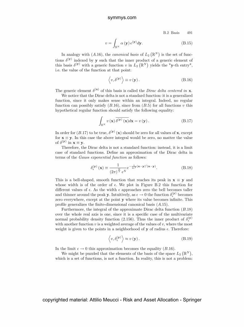
The generic element δ(x) of this basis is called the Dirac delta centered in x.We notice that the Dirac delta is not a standard function: it is a generalized

function, since it only makes sense within an integral. Indeed, no regularfunction can possibly satisfy (B.16), since from (B.5) for all functions v thishypothetical regular function should satisfy the following equality:Z

RNv (x) δ(y) (x)dx = v (y) . (B.17)

In order for (B.17) to be true, δ(y) (x) should be zero for all values of x, exceptfor x ≡ y. In this case the above integral would be zero, no matter the valueof δ(y) in x ≡ y.Therefore, the Dirac delta is not a standard function: instead, it is a limit

case of standard functions. Define an approximation of the Dirac delta interms of the Gauss exponential function as follows:

δ(y) (x) ≡ 1

(2π)N2 N

e−12 2 (x−y)0(x−y). (B.18)

This is a bell-shaped, smooth function that reaches its peak in x ≡ y andwhose width is of the order of . We plot in Figure B.2 this function fordifferent values of . As the width approaches zero the bell becomes tallerand thinner around the peak y. Intuitively, as → 0 the function δ(y) becomeszero everywhere, except at the point y where its value becomes infinite. Thisprofile generalizes the finite-dimensional canonical basis (A.15).Furthermore, the integral of the approximate Dirac delta function (B.18)

over the whole real axis is one, since it is a specific case of the multivariatenormal probability density function (2.156). Thus the inner product of δ(y)

with another function v is a weighted average of the values of v, where the mostweight is given to the points in a neighborhood of y of radius . Therefore:D

v, δ(y)E≈ v (y) . (B.19)

In the limit → 0 this approximation becomes the equality (B.16).We might be puzzled that the elements of the basis of the space L2

¡RN¢,

which is a set of functions, is not a function. In reality, this is not a problem:

symmys.com



( ) ( )δ y0.5 x

x1xN

( ) ( )δ y0.9 x

y

Fig. B.2. Approximation of the Dirac delta with Gaussian exponentials

we recall that in its definition we extended the space L2¡RN¢to include all

the natural limit operations, in such a way to make it complete, see (B.10).We summarize in the table below the analogies between the basis in the

finite-dimensional Euclidean vector space RN and in the infinite-dimensionalHilbert space L2

¡RN¢respectively.


basis©e(n)

ªn∈{1,...,N}

©e(y)

ªy∈RN

canonical basisDv, δ(n)

E= vn

Dv, δ(y)

E= v (y)

(B.20)

As an application, consider a random a variable X that takes on specificvalues x1,x2, . . . with finite probabilities px1 , px2 , . . . respectively. The vari-able X has a discrete distribution. In this situation no regular probabilitydensity function fX can satisfy (2.4). Indeed, if this were the case, the follow-ing equality would hold:

pxi = P {X = xi} =Z{xi}

fX (x) dx. (B.21)

Nevertheless, the integral of any regular function on the singleton {xi} isnull. On the other hand, if we express the probability density function fX asa generalized function this problem does not exist. Indeed, if we express fXin terms of the Dirac delta (B.16) as follows:

symmys.com


B.3 Linear operators 493

fX =Xi

pxiδ(xi), (B.22)

then this generalized function satisfies (B.21).In particular, consider the case of a discrete random variable that can only

take on one specific value ex with associated probability pex ≡ 1: this is not arandom variable, as the outcome of its measurement is known with certainty.Instead, it is a constant vector ex. The formalism of generalized functions allowsus to treat constants as special cases of a random variable. The visualizationof the probability density function of this "not-too-random" variable in termsof the regularized Dirac delta is a bell-shaped function centered around ex thatspikes to infinity as the approximation becomes exact.

B.3 Linear operators

Consider in analogy with (A.17) a transformation A that maps functions vof the Hilbert space L2

¡RN¢into functions that might belong to the same

Hilbert space, or to some other space of functions F :

A : v ∈ L2¡RN¢7→ u ≡ A [v] ∈ F . (B.23)

In the context of functional analysis, such transformations are called func-tionals or operators and generalize the finite-dimensional concept of function.In analogy with (A.18), a functional A is called a linear operator if it

preserves the sum and the multiplication by a scalar:

A [u+ v] = A [u] +A [v] (B.24)

A [αv] = αA [v] .

Geometrically, this means that infinite-dimensional parallelotopes are mappedinto infinite-dimensional parallelotopes, as represented in Figure A.3.

For example, consider the differentiation operator :

Dn [v] (x) ≡∂v (x)

∂xn. (B.25)

This operator is defined on a subset of smooth functions in L2¡RN¢. It is easy

to check that the differentiation operator is linear.

The inverse A−1 of a linear operator A is the functional that applied eitherbefore or after the linear operator A cancels the effect of the operator A. Inother words, in analogy with (A.20), for all functions v the inverse functionalA−1 satisfies: ¡

A−1 ◦A¢[v] = v =

¡A ◦A−1

¢[v] . (B.26)

symmys.com



As in the finite-dimensional case, in general the inverse transformation is notdefined. If it is defined, it is linear.

For example, consider the integration operator , defined as follows:

In [v] (x) ≡Z xn

−∞v (x1, . . . , zn, . . . xN ) dzn (B.27)

The fundamental theorem of calculus states that the integration operator isthe inverse of the differentiation operator (B.25). It is easy to check that theintegration operator is linear.

B.3.1 Kernel representations

In Appendix A.3.1 we saw that in the finite-dimensional case every lineartransformation A admits a matrix representation Amn. Therefore we expectthat every linear operator on L2

¡RN¢be expressible in terms of a continuous

version of a matrix. By means of the notational analogies of Table B.4 andTable B.11 this "continuous" matrix must be an integral kernel , i.e. a functionA (y,x) such that

A [v] (y) ≡ZRN

A (y,x) v (x) dx, (B.28)

which parallels (A.25). Such a representation does not exist in general. Theoperators that admit a kernel representation are called Hilbert-Schmidt oper-ators. Nevertheless, we can always find and use an approximate kernel, whichbecomes exact in a limit sense.

For example the kernel of the differentiation operator (B.25) is not de-fined (we consider the one-dimensional case for simplicity). Nevertheless, thefollowing kernel is well defined:

D (y, x) ≡ 1³δ(y+ ) (x)− δ(y) (x)

´, (B.29)

where δ(y) is the one-dimensional approximate Dirac delta (B.18). In the limit→ 0 we obtain:

lim→0

ZRD (y, x) v (x) dx = [Dv] (y) . (B.30)

Therefore (B.29) is the kernel representation of the differentiation operatorin a limit sense.

B.3.2 Unitary operators

Unitary operators are the generalization of rotations to the infinite-dimensionalworld of functional analysis. Therefore, in analogy with (A.30), an operator U

symmys.com


B.3 Linear operators 495

is unitary if it does not alter the length, i.e. the norm (B.8), of any functionin L2

¡RN¢:

kU [v]k = kvk . (B.31)

For example, it is immediate to check that the reflection operator definedbelow is unitary:

Refl [v] (x) ≡ v (−x) . (B.32)

Similarly the shift operator defined below is unitary:

Shifta [v] (x) ≡ v (x− a) . (B.33)

The most notable application of unitary operators is the Fourier trans-form. This transformation is defined in terms of its kernel representation asfollows:

F [v] (y) ≡ZRN

eiy0xv (x) dx. (B.34)

We prove below that for all functions in L2¡RN¢the following result holds:

kF [v]k = (2π)N2 kvk . (B.35)

Therefore the Fourier transform is a (rescaled) unitary operator.

For example, consider the normal probability density function (2.156):

fNµ,Σ (x) ≡1

(2π)N2 |Σ|

12

e−12 (µ−x)0Σ−1(µ−x). (B.36)

From (2.14), the Fourier transform of the normal pdf is the characteristicfunction of the normal distribution. From (2.157) it reads:

FhfNµ,Σ

i(y) = eiµ

0y− 12y

0Σy. (B.37)

In particular from (B.37) and (B.18), i.e. the fact that in the limit Σ→ 0

the normal density fNx,Σ becomes the Dirac delta δ(x), we obtain the following

notable result:Fhδ(x)

i= exp (ix0·) . (B.38)

In a Euclidean space rotations are invertible and the inverse is a rotation.Similarly, a unitary operator is always invertible and the inverse is a unitaryoperator. Furthermore, in a Euclidean space the representation of the inverserotation is the transpose matrix, see (A.31). Similarly, it is possible to provethat the kernel representation of the inverse of a unitary transformation isthe complex conjugate of the kernel representation of the unitary operator. Informulas:

symmys.com



U−1 [v] (x) =ZRN

U (y,x)v (y) dy. (B.39)

By this argument, the inverse Fourier transform is defined in terms of itskernel representation as follows:

F−1 [v] (x) ≡ (2π)NZRN

e−ix0yv (y) dy, (B.40)

where the factor (2π)N appears because the Fourier transform is a rescaledunitary transformation.In particular, inverting (B.38) and substituting v (y) ≡ eiz

0y in (B.40) weobtain the following useful identity:

δ(z) (x) = F−1 [exp (iz0·)] (x) = (2π)NZRN

ei(z−x)0ydy. (B.41)

Using this identity we can show that the Fourier transform is a rescaled unitarytransformation. Indeed:

kF [v]k2 ≡ZRN

·ZRN

eiy0xv (x) dx

¸ ·ZRN

eiy0zv (z) dz

¸dy

=

ZRN

ZRN

µZRN

e(iy0(x−z))dy

¶v (x) v (z)dxdz (B.42)

= (2π)NZRN

ZRN

δ(z) (x) v (x) v (z)dxdz = (2π)N kvk2 .

B.4 Regularization

In the Hilbert space of functions L2¡RN¢it is possible to define another

operation that turns out very useful in applications.The convolution of two functions u and v in this space is defined as follows:

[u ∗ v] (x) ≡ZRN

u (y) v (x− y) dy. (B.43)

The convolution shares many of the features of the multiplication betweennumbers. Indeed it is commutative, associative and distributive:

u ∗ v = v ∗ u(u ∗ v) ∗ z = u ∗ (v ∗ z) (B.44)

(u+ v) ∗ z = u ∗ z + v ∗ z.

Furthermore, the Fourier transform (B.34) of the convolution of two functionsis the product of the Fourier transforms of the two functions:

F [u ∗ v] = F [u]F [v] . (B.45)

symmys.com


B.4 Regularization 497

This follows from the series of identities:

F [u ∗ v] (y) ≡ZRN

eiy0x [u ∗ v] (x) dx

=

ZRN

u (z)

·ZRN

eiy0xv (x− z) dx

¸dz (B.46)

=

ZRN

u (z)heiy

0zF [v] (y)idz

= F [v] (y)F [u] (y) .

An important application of the convolution stems from the immediateresult that the Dirac delta (B.16) centered in zero is the neutral element ofthe convolution: h

δ(0) ∗ vi= v. (B.47)

By approximating the Dirac delta with the smooth function δ(0) defined in(B.18), we obtain from (B.47) an approximate expression for a generic func-tion v, which we call the regularization of v with bandwidth :

v ≡hδ(0) ∗ v

i≈ v. (B.48)

From (B.43), the regularization of v reads explicitly as follows:

v (x) ≡ 1

(2π)N2 N

ZRN

e−(y−x)0(y−x)

2 2 v (y) dy. (B.49)

Due to the bell-shaped profile of the Gaussian exponential in the above in-tegral, the regularized function v (x) is a moving average of v (x) with itssurrounding values: the effect of the surrounding values fades away as theirdistance from x increases. The size of the "important" points that deter-mine the moving average is determined by the bandwidth of the bell-shapedGaussian exponential.The regularization (B.49) becomes exact as the bandwidth tends to zero:

indeed, in the limit where tends to zero, the Gaussian exponential tends tothe Dirac delta, and we recover (B.47). Furthermore, the regularized functionv is smooth: indeed, since the Gaussian exponential is smooth, the right handside of (B.49) can be derived infinite times with respect to x.To become more acquainted with the regularization technique we use it

to compute the derivative of the Heaviside function H(y) defined in (B.73).The partial derivative of the Heaviside function along any coordinate is zeroeverywhere, except in y, where the limit that defines the partial derivativediverges to infinity. This behavior resembles that of the Dirac delta δ(y), sowe are led to conjecture that the combined partial derivatives of the Heavisidefunction are the Dirac delta:

(D1 ◦ · · · ◦DN )hH(y)

i= δ(y). (B.50)

symmys.com



We can verify this conjecture with the newly introduced operations. First wenotice that in general the convolution of a function with the Heaviside functionis the combined integral (B.27) of that function:³

v ∗H(y)´(x) ≡

ZRN

v (z)H(y) (x− z) dz (B.51)

=

Z x1−y1

−∞· · ·Z xN−yN

−∞v (z) dz = (I1 ◦ · · · ◦ IN ) [v] (x− y) .

Applying this result to the regularization (B.48) of the Heaviside function andrecalling from (B.27) that the integration is the inverse of the differentiation,we obtain:

(D1 ◦ · · · ◦DN )hH(y)

i≡ (D1 ◦ · · · ◦DN )

hH(y) ∗ δ(0)

i(B.52)

= (D1 ◦ · · · ◦DN )h(I1 ◦ · · · ◦ IN )

hδ(y)

ii= δ(y).

Taking the limit → 0 we obtain the proof of the conjecture (B.50).

Using (B.50) we can compute the cumulative distribution function of adiscrete distribution, whose probability density function is (B.22). Indeed,from the definition of cumulative distribution function (2.10) we obtain:

FX ≡ (I1 ◦ · · · ◦ IN )"Xxi

pxiδ(xi)

#=Xxi

pxiH(xi), (B.53)

where we used the fact that the integration operator is linear.

An important application of the regularization technique concerns theprobability density function fX of a generic random variable X. Indeed, con-sider the regularization (B.49) of fX, which can be a very irregular function,or even a generalized function:

fX; (x) ≡1

(2π)N2 N

ZRN

e−(y−x)0(y−x)

2 2 f (y) dy. (B.54)

It is immediate to check that fX; is strictly positive everywhere and integratesto one over the entire domain: therefore it is a probability density function.Furthermore, we notice that in general the probability density function

fX of a random variable X is not univocally defined. Indeed, from its verydefinition (2.4) the probability density function only makes sense within anintegral. For instance, if we change its value at one specific point, the ensuingaltered probability density is completely equivalent to the original one. Moreprecisely, a probability density function is an equivalence class of functionsthat are identical almost everywhere, i.e. they are equal to each other exceptpossibly on a set of zero probability (such as one point). The regularization

symmys.com


B.5 Expectation operator 499

technique (B.54) provides a univocally defined, smooth and positive proba-bility density function.Therefore, whenever needed, we can replace the original probability density

function fX with its regularized version fX; , which is smooth and approxi-mates the original probability density function fX to any degree of accuracy.If necessary, we can eventually consider the limit → 0 in the final solution toour problem, in order to recover an exact answer that does not depend on thebandwidth . Nevertheless, from a more "philosophical" point of view, in mostcases we do not need to consider the limit → 0 in the final solution. Indeed,in most applications it is impossible to distinguish between a statistical modelbased on the original probability density function fX and one based on theregularized probability density function fX; , provided that the bandwidth issmall enough. Therefore it becomes questionable which of the two probabilitydensity functions is the "real" and which is the "approximate" model.

B.5 Expectation operator

Consider a random variable X, whose probability density function is fX. Con-sider a new random variable Y defined in terms of a generic function g of theoriginal variable X:

Y ≡ g (X) . (B.55)

We recall that the set of functions of the random variable X is a vector space,since sum and multiplication by a scalar are defined in a natural way as in(B.2) and (B.3) respectively.To get a rough idea of the possible outcomes of the random variable Y de-

fined in (B.55) it is intuitive to weigh each possible outcome by its respectiveprobability. This way we are led to the definition of the expectation operatorassociated with the distribution fX. This operator associates with any func-tion of a random variable the probability-weighted average of all its possibleoutcomes:

E {g (X)} ≡ EX {g} ≡ZRN

g (x) fX (x) dx. (B.56)

To simplify the notation we might at times drop the symbol X. From thisdefinition it is immediate to check that the expectation operator is linear, i.e.it satisfies (B.24).The expectation operator endows the functions of X with a norm, and

thus with the structure of Banach space. Indeed, consider an arbitrary positivenumber p. We define the p-norm of g as follows:

kgkX;p ≡ (EX {|g|p})

1p . (B.57)

When defined, it is possible to check that this is indeed a norm, as it satisfiesthe properties (A.7). In order to guarantee that the norm is defined, we restrictthe generic space of functions of X to the following subspace:

symmys.com



LpX ≡ {g such that EX {|g|p} <∞} . (B.58)

Given the norm, we can define the distance kg − hkX;p between two genericfunctions g and h in LpX.The space L2X is somewhat special, as it can also be endowed with the

following inner product:hg, hiX ≡ E

©ghª. (B.59)

It is easy to check that in L2X the norm is induced by the inner product:

k·kX;2 =qh·, ·iX. (B.60)

Therefore, L2X is a Hilbert space and in addition to the properties (A.7) alsothe Cauchy-Schwartz inequality (A.8) is satisfied:

|hg, hiX| ≤ kgkX;2 khkX;2 . (B.61)

As in (A.9)-(A.10) the equality in this expression holds if and only if g ≡ αhalmost everywhere for some scalar α. If the scalar α is positive:

hg, hiX = kgkX;2 khkX;2 ; (B.62)

if the scalar α is negative:

hg, hiX = − kgkX;2 khkX;2 . (B.63)

It is easy to check that the operator h·, ·iX is, like all inner products,symmetric and bilinear . Explicitly, this means that for all functions g and hin L2X:

hg, hiX = hh, giX ; (B.64)

and that for any function g in L2X the application hg, ·iX is linear. This impliesin particular that the inner product of a linear combination of functions withitself can be expressed as follows:*

MXm=1

αmgm,MXm=1

αmgm

+X

= α0Sα, (B.65)

where S is an M ×M matrix:

Smn ≡ hgm, gniX . (B.66)

It is easy to check that this matrix is symmetric, i.e. it satisfies (A.51), andpositive, i.e. it satisfies (A.52).In particular, if we consider the functions

gm (X) ≡ Xm − E {Xm} (B.67)

symmys.com


B.6 Some special functions 501

the matrix (B.66) becomes the covariance matrix (2.67):

Smn ≡ hXm − E {Xm} ,Xn − E {Xn}iX (B.68)

= Cov {Xm,Xn} .

The Cauchy-Schwartz inequality (B.61) in this context reads:

|Cov {Xm,Xn}| ≤ Sd {Xm}Sd {Xn} . (B.69)

In particular, from (B.62) and the affine equivariance of the expected value(2.56) we obtain:

Cov {Xm,Xn} = Sd {Xm}Sd {Xn}⇔ Xm = a+ bXn, (B.70)

where a is a scalar and b is a positive scalar. Similarly, from (B.63) and theaffine equivariance of the expected value (2.56) we obtain:

Cov {Xm,Xn} = −Sd {Xm}Sd {Xn}⇔ Xm = a− bXn, (B.71)

where a is a scalar and b is a positive scalar. These properties allow us todefine the correlation matrix.

B.6 Some special functions

We conclude with a list of special functions that recur throughout the text.See Abramowitz and Stegun (1974) and mathworld.com for more information.The indicator function of a set S ∈ RN is defined as follows:

IS (x) ≡½1 if x ∈ S0 if x /∈ S. (B.72)

The Heaviside function H(y) is a step function:

H(y) (x) ≡½1 where x1 ≥ y1, . . . , xN ≥ yN0 otherwise.

(B.73)

We can define equivalently the Heaviside function in terms of the indicatorfunction (B.72) as follows:

H(y) ≡ I[y1,+∞)×···[yN ,+∞). (B.74)

The error function is defined as the integral of the Gaussian exponential:

erf (x) ≡ 2√π

Z x

0

e−u2

du. (B.75)

The error function is odd:

symmys.com



erf (−x) = − erf (x) . (B.76)

Furthermore, the error function is normalized in such a way that:

erf (∞) = 1. (B.77)

This implies the following relation for the complementary error function:

erfc (x) ≡ 2√π

Z +∞

x

e−u2

du = 1− erf (x) . (B.78)

The factorial is a function defined only on integer values:

n! ≡ 1× 2× 3× · · · × (n− 1)× n. (B.79)

The gamma function is defined by the following integral:

Γ (a) ≡Z +∞

0

ua−1 exp (−u) du. (B.80)

The gamma function is an extension to the complex and real numbers ofthe factorial. Indeed it is easy to check from the definition (B.80) that thefollowing identity holds:

Γ (n) = (n− 1)!. (B.81)

For half-integer arguments, it can be proved that the following identity holds:

Γ³n2

´=(n− 2) (n− 4) · · ·n0

√π

2n−12

, (B.82)

where n0 ≡ 1 if n is odd and n0 ≡ 2 if n is even.The lower incomplete gamma function is defined as follows:

γ (x; a) ≡Z x

0

ua−1e−udu. (B.83)

The upper incomplete gamma function is defined as follows:

Γ (x; a) ≡Z +∞

x

ua−1e−udu. (B.84)

The lower regularized gamma function is defined as follows:

P (x; a) ≡ γ (x; a)

Γ (a). (B.85)

The upper regularized gamma function is defined as follows:

Q (x; a) ≡ Γ (x; a)

Γ (a). (B.86)

symmys.com


B.6 Some special functions 503

The regularized gamma functions satisfy:

P (x; a) +Q (x; a) = 1. (B.87)

The beta function is defined by the following integral:

B (a, b) ≡Z 1

0

ua−1 (1− u)b−1 du. (B.88)

The beta function is related to the gamma function through this identity:

B (a, b) =Γ (a)Γ (b)

Γ (a+ b). (B.89)

The incomplete beta function is defined by the following integral:

B (x; a, b) ≡Z x

0

ua−1 (1− u)b−1 du. (B.90)

The regularized beta function is a normalized version of the incomplete betafunction:

I (x; a, b) ≡ B (x; a, b)

B (a, b). (B.91)

Therefore the regularized beta function satisfies

I (0; a, b) = 0, I (1; a, b) = 1. (B.92)

The Bessel functions of first, second, and third kind are solutions to thefollowing differential equation:

x2d2w

dx2+ x

dw

dx+¡x2 − ν2

¢w = 0.

In particular, the Bessel function of the second kind admits the followingintegral representation, see Abramowitz and Stegun (1974) p. 360:

Yν (x) =1

π

Z π

0

sin (x sin (θ)− νθ) dθ (B.93)

− 1π

Z +∞

0

¡eνu + e−νu cos (νπ)

¢ex sinh(u)du.

symmys.com


symmys.com


Documents

B Functional Analysis - ARPM _ Attilio Meucci - Risk and... · B Functional Analysis In this appendix we provide a very loose review of linear functional analysis. Due to the extension