B-trees - Hashing. 11.2Database System Concepts Review: B-trees and B+-trees Multilevel, disk-aware, balanced index methods primary or secondary dense

B-trees - HashingB-trees - Hashing

11.2Database System Concepts

Review: B-trees and B+-treesReview: B-trees and B+-trees

Multilevel, disk-aware, balanced index methods

•primary or secondary• dense or sparse•supports selection and range queries

B+-trees: most common indexing structure in databases

• all actual values stored on leaf-nodes.

Optimality: space O(N/B), updates O(log B (N/B)), queries O(log B (N/B)+K/B) (B is the fan out of a node)


Root

B+Tree Example Order= 4

100

120

150

180

30

3 5 11

30

35

100

101

110

120

130

150

156

179

180

200


Full node min. node

Non-leaf

Leaf

n=4

12

01

50

18

0

30

3 5 11

30

35


B+tree rulesB+tree rules tree of order tree of order nn

(1) All leaves at same lowest level (balanced tree)

(2) Pointers in leaves point to records except for “sequence pointer”

(3) Number of pointers/keys for B+tree

Non-leaf(non-root) n n-1 n/2 n/2- 1

Leaf(non-root) n n-1

Root n n-1 2 1

Max Max Min Min ptrs keys ptrs keys

(n-1)/2(n-1)/2


Insert into B+treeInsert into B+tree

(a) simple case

space available in leaf

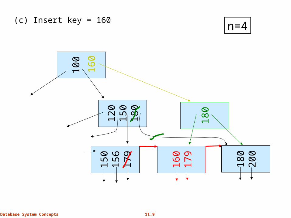
(b) leaf overflow

(c) non-leaf overflow

(d) new root


(a) Insert key = 32 n=43 5 11

30

31

30

100

32


(a) Insert key = 7 n=4

3 5 11

30

31

30

100

3 5

7

7


(c) Insert key = 160n=4

10

0

120

150

180

150

156

179

180

200

160

18

0

160

179


(d) New root, insert 45 n=4

10

20

30

1 2 3 10

12

20

25

30

32

40

40

45

40

30new root


(a) Simple case - no example

(b) Coalesce with neighbor (sibling)

(c) Re-distribute keys

(d) Cases (b) or (c) at non-leaf

Deletion from B+treeDeletion from B+tree


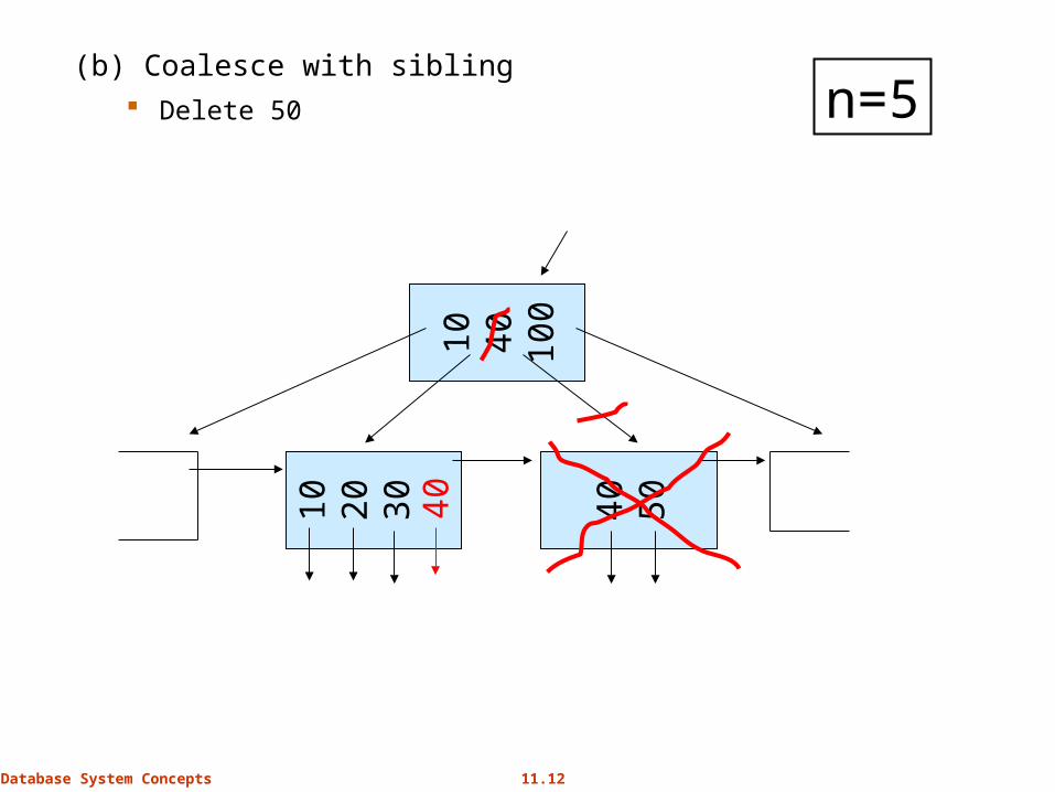
(b) Coalesce with sibling Delete 50

10

40

100

10

20

30

40

50

n=5

40


(c) Redistribute keys Delete 50

10

40

100

10

20

30

35

40

50

n=5

35

35


40

45

30

37

25

26

20

22

10

141 3

10

20

30

40

(d) Non-leaf coalesce Delete 37 n=5

40

30

25

25

new root


Selection QueriesSelection Queries

Yes! Hashing

static hashing

dynamic hashing

B+-tree is perfect, but....

to answer a selection query (ssn=10) needs to traverse a full path.

In practice, 3-4 block accesses (depending on the height of the tree, buffering)

Any better approach?


HashingHashing

Hash-based indexes are best for equality selections. Cannot support range searches.

Static and dynamic hashing techniques exist; trade-offs similar to ISAM vs. B+ trees.


Static HashingStatic Hashing # primary pages fixed, allocated sequentially, never de-allocated;

overflow pages if needed.

h(k) MOD N= bucket to which data entry with key k belongs. (N = # of buckets)

h(key) mod N

hkey

Primary bucket pages Overflow pages

10

N-1


Static Hashing (Contd.)Static Hashing (Contd.)

Buckets contain data entries.

Hash fn works on search key field of record r. Use its value MOD N to distribute values over range 0 ... N-1. h(key) = (a * key + b) usually works well.

a and b are constants; lots known about how to tune h.

Long overflow chains can develop and degrade performance. extendable and Linear Hashing: Dynamic techniques to fix this problem.


extendable Hashingextendable Hashing

Situation: Bucket (primary page) becomes full. Why not re-organize file by doubling # of buckets? Reading and writing all pages is expensive!

Idea: Use directory of pointers to buckets, double # of buckets by doubling the directory, splitting just the bucket that overflowed! Directory much smaller than file, so doubling it is much cheaper. Only one

page of data entries is split. No overflow page!

Trick lies in how hash function is adjusted!


ExampleExample

13*00

0110

11

2

2

1

2

LOCAL DEPTH

GLOBAL DEPTH

DIRECTORY

Bucket A

Bucket B

Bucket C10*

1* 7*

4* 12* 32* 16*

5*

we denote r by h(r).

• Directory is array of size 4.• Bucket for record r has entry with index = `global depth’ least

significant bits of h(r);– If h(r) = 5 = binary 101, it is in bucket pointed to by 01.– If h(r) = 7 = binary 111, it is in bucket pointed to by 11.


Handling InsertsHandling Inserts

Find bucket where record belongs. If there’s room, put it there. Else, if bucket is full, split it:

increment local depth of original page allocate new page with new local depth re-distribute records from original page. add entry for the new page to the directory


Example: Insert 21, then 19, 15Example: Insert 21, then 19, 15

13*00

0110

11

2

2

LOCAL DEPTH

GLOBAL DEPTH

DIRECTORY

Bucket A

Bucket B

Bucket C

2Bucket D

DATA PAGES

10*

1* 7*

24* 12* 32* 16*

15*7* 19*

5*

21 = 10101

19 = 10011

15 = 01111

1221*


24* 12* 32*16*

Insert Insert hh(r)=20 (Causes Doubling)(r)=20 (Causes Doubling)

00

01

10

11

2 2

2

2

LOCAL DEPTH

GLOBAL DEPTHBucket A

Bucket B

Bucket C

Bucket D

1* 5* 21*13*

10*

15* 7* 19*

(`split image'of Bucket A)

20*

3

Bucket A24* 12*

of Bucket A)

3

Bucket A2(`split image'

4* 20*12*

2

Bucket B1* 5* 21*13*

10*

2

19*

2

Bucket D15* 7*

3

32*16*

LOCAL DEPTH

000

001

010

011

100

101

110

111

3

GLOBAL DEPTH

3

32*16*


Points to NotePoints to Note

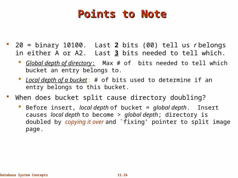
20 = binary 10100. Last 2 bits (00) tell us r belongs in either A or A2. Last 3 bits needed to tell which. Global depth of directory: Max # of bits needed to tell which bucket an entry

belongs to.

Local depth of a bucket: # of bits used to determine if an entry belongs to this bucket.

When does bucket split cause directory doubling? Before insert, local depth of bucket = global depth. Insert causes local depth

to become > global depth; directory is doubled by copying it over and `fixing’ pointer to split image page.


Directory DoublingDirectory Doubling

00

01

10

11

2

Why use least significant bits in directory? Allows for doubling via copying!

3

000

001

010

011

100

101

110

111

vs.

0

1

1

6*6*

6*

6 = 110

00

10

01

11

2

3

0

1

1

6*6*

6*

6 = 110000

100

010

110

001

101

011

111

Least Significant Most Significant


Comments on extendable HashingComments on extendable Hashing

If directory fits in memory, equality search answered with one disk access; else two. 100MB file, 100 bytes/rec, 4K pages contains 1,000,000 records (as data

entries) and 25,000 directory elements; chances are high that directory will fit in memory.

Directory grows in spurts, and, if the distribution of hash values is skewed, directory can grow large.

Multiple entries with same hash value cause problems!

Delete: If removal of data entry makes bucket empty, can be merged with `split image’. If each directory element points to same bucket as its split image, can halve directory.


Extendable Hashing vs. Other SchemesExtendable Hashing vs. Other Schemes

Benefits of extendable hashing: Hash performance does not degrade with growth of file Minimal space overhead

Disadvantages of extendable hashing Extra level of indirection to find desired record Bucket address table may itself become very big (larger than

memory) Cannot allocate very large contiguous areas on disk either Solution: B+-tree structure to locate desired record in bucket address

table

Changing size of bucket address table is an expensive operation

Linear hashing is an alternative mechanism Allows incremental growth of its directory (equivalent to bucket

address table) At the cost of more bucket overflows


Comparison of Ordered Indexing and HashingComparison of Ordered Indexing and Hashing

Cost of periodic re-organization Relative frequency of insertions and deletions Is it desirable to optimize average access time at the expense of

worst-case access time? Expected type of queries:

Hashing is generally better at retrieving records having a specified value of the key.

If range queries are common, ordered indices are to be preferred

In practice: PostgreSQL supports hash indices, but discourages use due to poor

performance Oracle supports B+trees, static hash organization, but not hash

indices SQLServer supports only B+-trees


Bitmap IndicesBitmap Indices

Bitmap indices are a special type of index designed for efficient querying on multiple keys

Very effective on attributes that take on a relatively small number of distinct values E.g. gender, country, state, …

E.g. income-level (income broken up into a small number of levels such as 0-9999, 10000-19999, 20000-50000, 50000- infinity)

A bitmap is simply an array of bits For each gender, we associate a bitmap, where each bit represents

whether or not the corresponding record has that gender.


Bitmap Indices (Cont.)Bitmap Indices (Cont.)

In its simplest form a bitmap index on an attribute has a bitmap for each value of the attribute Bitmap has as many bits as records

In a bitmap for value v, the bit for a record is 1 if the record has the value v for the attribute, and is 0 otherwise



Bitmap indices are useful for queries on multiple attributes not particularly useful for single attribute queries

Queries are answered using bitmap operations Intersection (and) Union (or) Complementation (not)

Each operation takes two bitmaps of the same size and applies the operation on corresponding bits to get the result bitmap E.g. 100110 AND 110011 = 100010

100110 OR 110011 = 110111 NOT 100110 = 011001

Males with income level L1: And’ing of Males bitmap with Income Level L1 bitmap

10010 AND 10100 = 10000 Can then retrieve required tuples. Counting number of matching tuples is even faster



Bitmap indices generally very small compared with relation size E.g. if record is 100 bytes, space for a single bitmap is 1/800 of space

used by relation. If number of distinct attribute values is 8, bitmap is only 1% of relation size

Deletion needs to be handled properly Existence bitmap to note if there is a valid record at a record location

Needed for complementation not(A=v): (NOT bitmap-A-v) AND ExistenceBitmap

Should keep bitmaps for all values, even null value To correctly handle SQL null semantics for NOT(A=v):

intersect above result with (NOT bitmap-A-Null)


Efficient Implementation of Bitmap OperationsEfficient Implementation of Bitmap Operations

Bitmaps are packed into words; a single word and (a basic CPU instruction) computes and of 32 or 64 bits at once E.g. 1-million-bit maps can be and-ed with just 31,250 instruction

Counting number of 1s can be done fast by a trick: Use each byte to index into a precomputed array of 256 elements

each storing the count of 1s in the binary representation Can use pairs of bytes to speed up further at a higher memory cost

Add up the retrieved counts

Bitmaps can be used instead of Tuple-ID lists at leaf levels of B+-trees, for values that have a large number of matching records Worthwhile if > 1/64 of the records have that value, assuming a

tuple-id is 64 bits

Above technique merges benefits of bitmap and B+-tree indices


Index Definition in SQLIndex Definition in SQL

Create a B-tree index (default in most databases)create index <index-name> on <relation-name>

(<attribute-list>)

-- create index b-index on branch(branch_name)

-- create index ba-index on branch(branch_name, account) -- concatenated index

-- create index fa-index on branch(func(balance, amount)) – function index

Use create unique index to indirectly specify and enforce the condition that the search key is a candidate key.

Hash indexes: not supported by every database (but implicitly in joins,…) PostgresSQL has it but discourages due to performance

Create a bitmap indexcreate bitmap index <index-name> on <relation-name>

(<attribute-list>)

- For attributes with few distinct values

- Mainly for decision-support(query) and not OLTP (do not support updates efficiently)

To drop any index drop index <index-name>

End of ChapterEnd of Chapter


Partitioned HashingPartitioned Hashing

Hash values are split into segments that depend on each attribute of the search-key.

(A1, A2, . . . , An) for n attribute search-key

Example: n = 2, for customer, search-key being (customer-street, customer-city)

search-key value hash value(Main, Harrison) 101 111(Main, Brooklyn) 101 001(Park, Palo Alto) 010 010(Spring, Brooklyn) 001 001(Alma, Palo Alto) 110 010

To answer equality query on single attribute, need to look up multiple buckets. Similar in effect to grid files.


Grid FilesGrid Files

Structure used to speed the processing of general multiple search-key queries involving one or more comparison operators.

The grid file has a single grid array and one linear scale for each search-key attribute. The grid array has number of dimensions equal to number of search-key attributes.

Multiple cells of grid array can point to same bucket

To find the bucket for a search-key value, locate the row and column of its cell using the linear scales and follow pointer


Example Grid File for Example Grid File for accountaccount


Queries on a Grid FileQueries on a Grid File

A grid file on two attributes A and B can handle queries of all following forms with reasonable efficiency

(a1 A a2)

(b1 B b2)

(a1 A a2 b1 B b2),.

E.g., to answer (a1 A a2 b1 B b2), use linear scales to find corresponding candidate grid array cells, and look up all the buckets pointed to from those cells.


Grid Files (Cont.)Grid Files (Cont.)

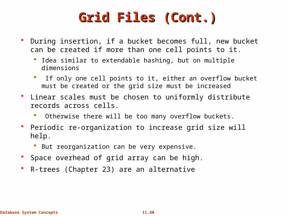
During insertion, if a bucket becomes full, new bucket can be created if more than one cell points to it. Idea similar to extendable hashing, but on multiple dimensions

If only one cell points to it, either an overflow bucket must be created or the grid size must be increased

Linear scales must be chosen to uniformly distribute records across cells. Otherwise there will be too many overflow buckets.

Periodic re-organization to increase grid size will help. But reorganization can be very expensive.

Space overhead of grid array can be high.

R-trees (Chapter 23) are an alternative


Linear HashingLinear Hashing

A dynamic hashing scheme that handles the problem of long overflow chains without using a directory.

Directory avoided in LH by using temporary overflow pages, and choosing the bucket to split in a round-robin fashion.

When any bucket overflows split the bucket that is currently pointed to by the “Next” pointer and then increment that pointer to the next bucket.


Linear Hashing – The Main IdeaLinear Hashing – The Main Idea

Use a family of hash functions h0, h1, h2, ...

hi(key) = h(key) mod(2iN)

N = initial # buckets

h is some hash function

hi+1 doubles the range of hi (similar to directory doubling)


Linear Hashing (Contd.)Linear Hashing (Contd.)

Algorithm proceeds in `rounds’. Current round number is “Level”.

There are NLevel (= N * 2Level) buckets at the beginning of a round

Buckets 0 to Next-1 have been split; Next to NLevel have not been split yet this round.

Round ends when all initial buckets have been split (i.e. Next = NLevel).

To start next round:

Level++;

Next = 0;


LH Search AlgorithmLH Search Algorithm

To find bucket for data entry r, find hLevel(r):

If hLevel(r) >= Next (i.e., hLevel(r) is a bucket that hasn’t been involved in a split this round) then r belongs in that bucket for sure.

Else, r could belong to bucket hLevel(r) or bucket hLevel(r) + NLevel must apply hLevel+1(r) to find out.


Example: Search 44 (11100), 9 (01001) Example: Search 44 (11100), 9 (01001)

0hh

1

Level=0, Next=0, N=4

00

01

10

11

000

001

010

011

PRIMARYPAGES

44* 36*32*

25*9* 5*

14* 18*10* 30*

31* 35* 11*7*

(This infois for illustrationonly!)


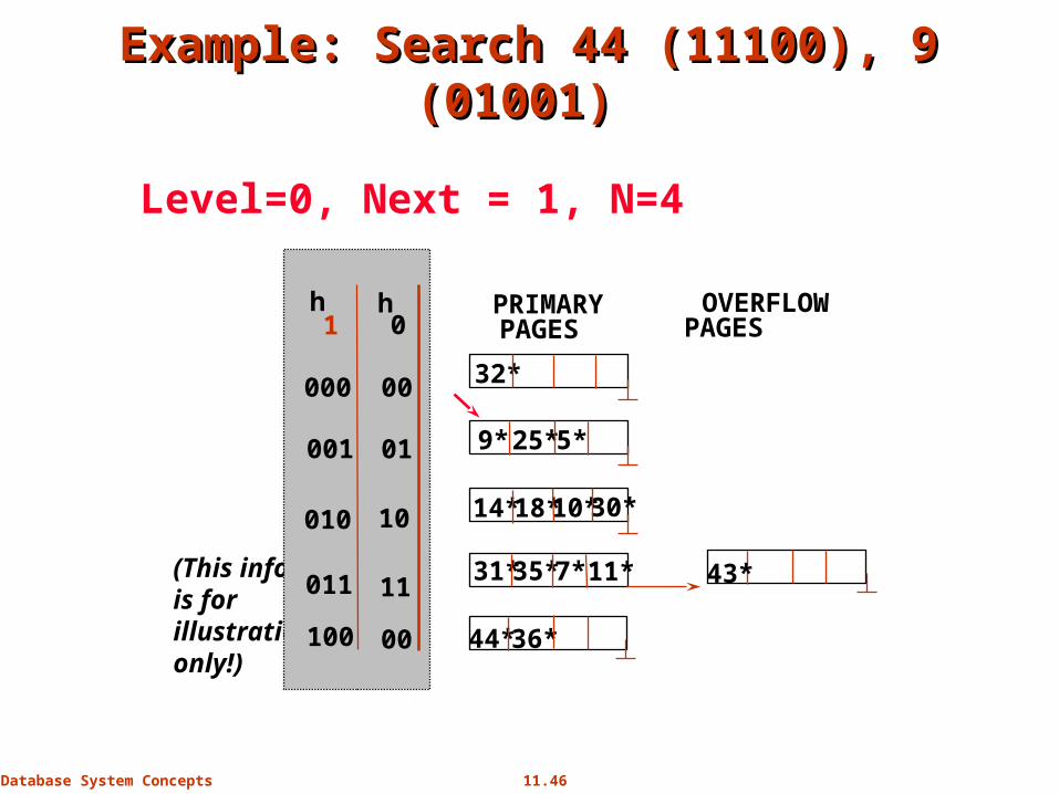
Level=0, Next = 1, N=4


0hh

1

00

01

10

11

000

001

010

011

PRIMARYPAGES

OVERFLOWPAGES

00100 44*36*

32*

25*9* 5*

14*18*10*30*

31*35* 11*7* 43*

Example: Search 44 (11100), 9 (01001) Example: Search 44 (11100), 9 (01001)


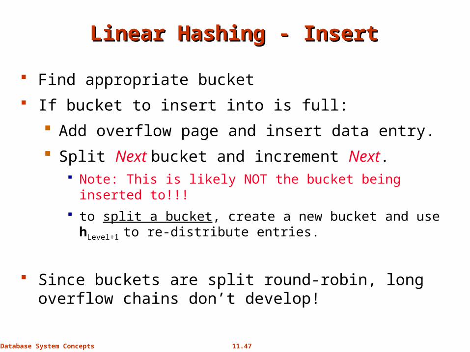
Linear Hashing - InsertLinear Hashing - Insert

Find appropriate bucket

If bucket to insert into is full:

Add overflow page and insert data entry.

Split Next bucket and increment Next. Note: This is likely NOT the bucket being inserted to!!!

to split a bucket, create a new bucket and use hLevel+1 to re-distribute entries.

Since buckets are split round-robin, long overflow chains don’t develop!


Example: Insert 43 (101011)Example: Insert 43 (101011)

0hh

1


Level=0, N=4

00

01

10

11

000

001

010

011

Next=0

PRIMARYPAGES

0hh

1

Level=0

00

01

10

11

000

001

010

011

Next=1

PRIMARYPAGES

OVERFLOWPAGES

00100

44* 36*32*

25*9* 5*

14* 18*10* 30*

31* 35* 11*7*

44*36*

32*

25*9* 5*

14*18*10*30*

31*35* 11*7* 43*



Example: End of a RoundExample: End of a Round

0hh1

22*

00

01

10

11

000

001

010

011

00100

Next=3

01

10

101

110

Level=0, Next = 3PRIMARYPAGES

OVERFLOWPAGES

32*

9*

5*

14*

25*

66* 10*18* 34*

35*31* 7* 11* 43*

44*36*

37*29*

30*

0hh1

37*

00

01

10

11

000

001

010

011

00100

10

101

110

Next=0

111

11

PRIMARYPAGES

OVERFLOWPAGES

11

32*

9* 25*

66* 18* 10* 34*

35* 11*

44* 36*

5* 29*

43*

14* 30* 22*

31*7*

50*

Insert 50 (110010)Level=1, Next = 0

Documents

B-trees - Hashing. 11.2Database System Concepts Review: B-trees and B+-trees Multilevel, disk-aware, balanced index methods primary or secondary dense