Embed Size (px)
Citation preview
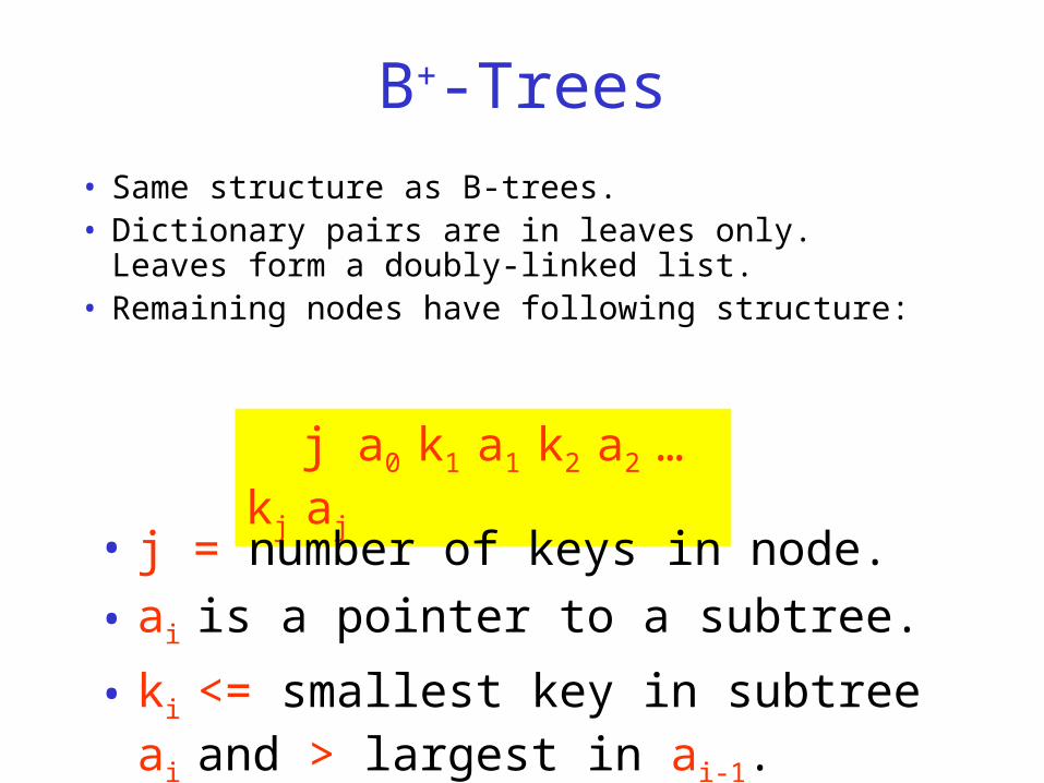
B+-Trees
• Same structure as B-trees.• Dictionary pairs are in leaves only. Leaves form a
doubly-linked list.• Remaining nodes have following structure:
j a0 k1 a1 k2 a2 … kj aj
• j = number of keys in node.
• ai is a pointer to a subtree.
• ki <= smallest key in subtree ai and > largest in ai-1.
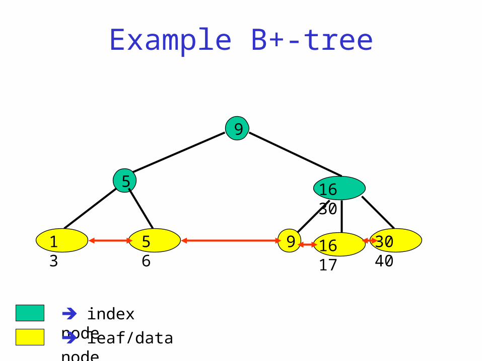
Example B+-tree
9
5
1 3 5 6 30 409 16 17
16 30
index node
leaf/data node
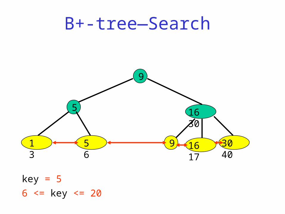
B+-tree—Search
9
5
1 3 5 6 30 409 16 17
16 30
key = 5
6 <= key <= 20
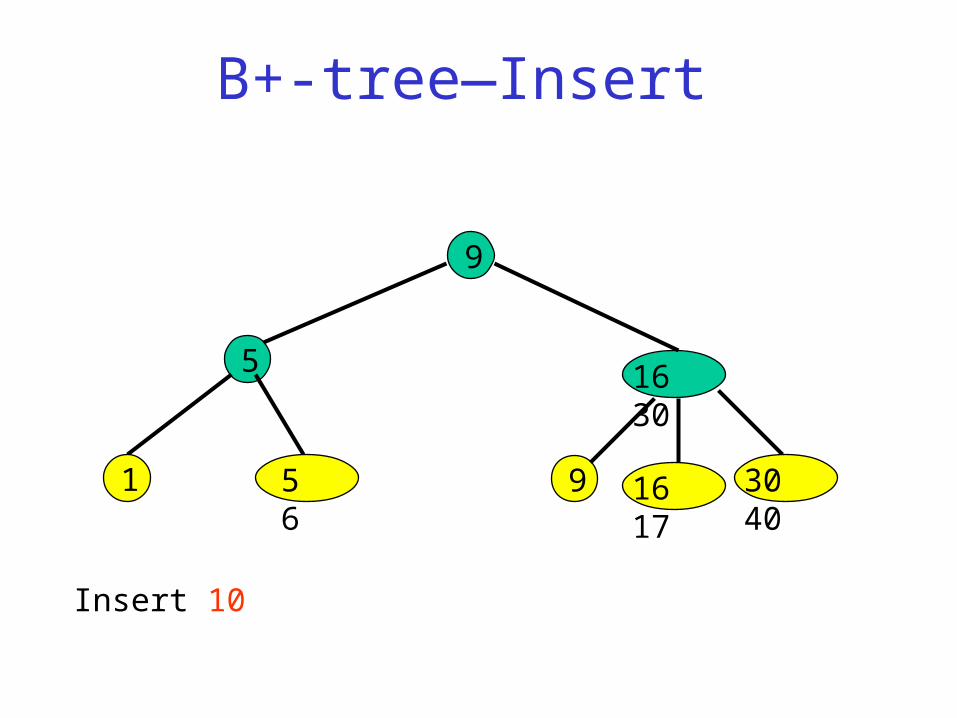
B+-tree—Insert
9
5
5 6 30 409 16 17
16 30
Insert 10
1
16 30
Insert9
5
1 3 5 6 30 409
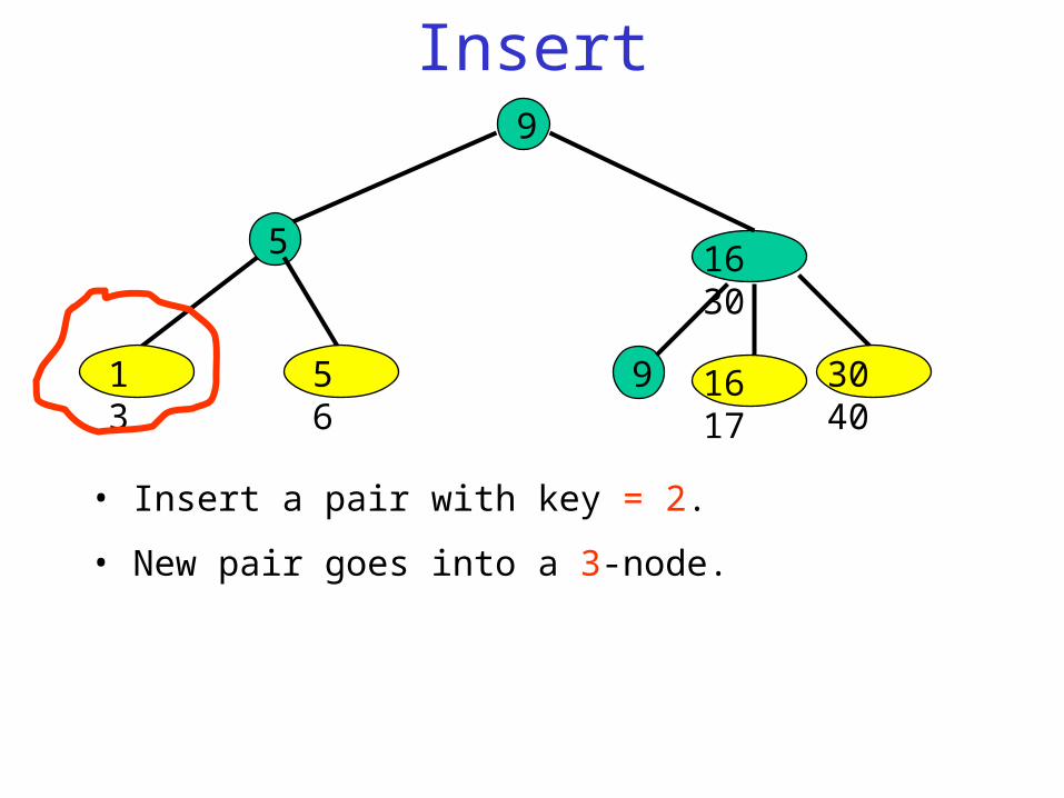
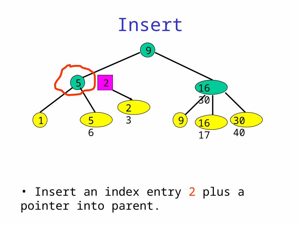
• Insert a pair with key = 2.
• New pair goes into a 3-node.
16 17
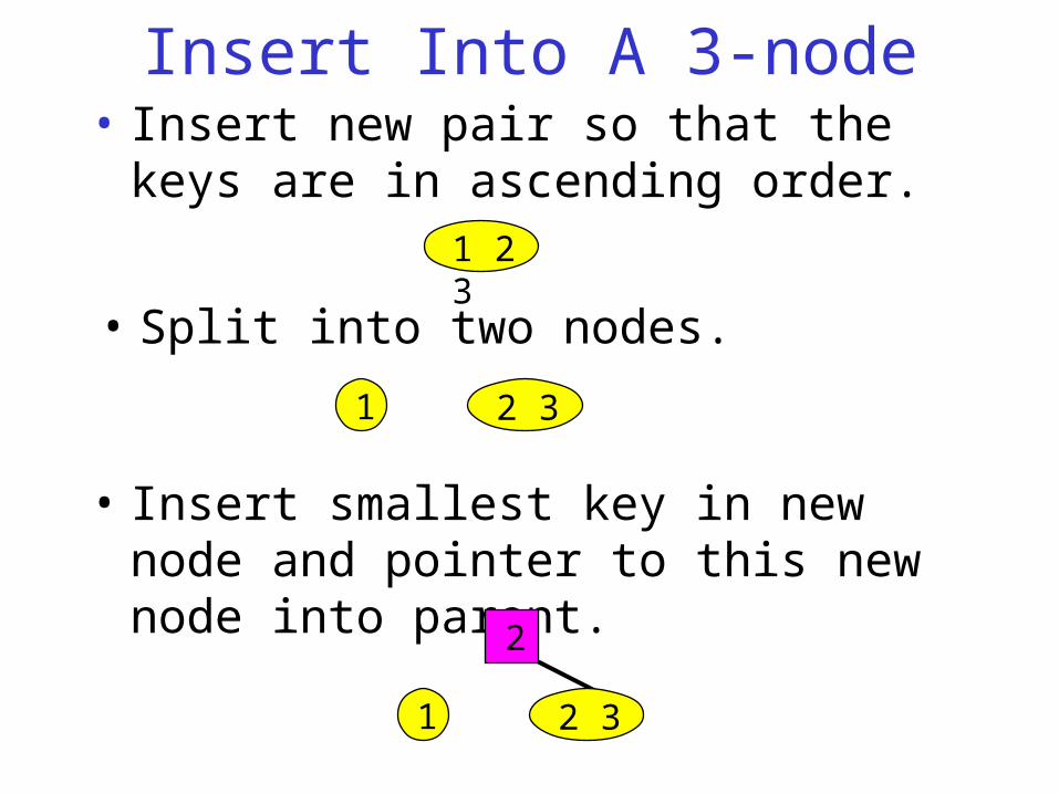
Insert Into A 3-node• Insert new pair so that the keys are in
ascending order.
• Split into two nodes.
2 31
1 2 3
• Insert smallest key in new node and pointer to this new node into parent.
2
2 31
9
Insert9
5
5 6 30 4016 17
2
• Insert an index entry 2 plus a pointer into parent.
2 31
16 30
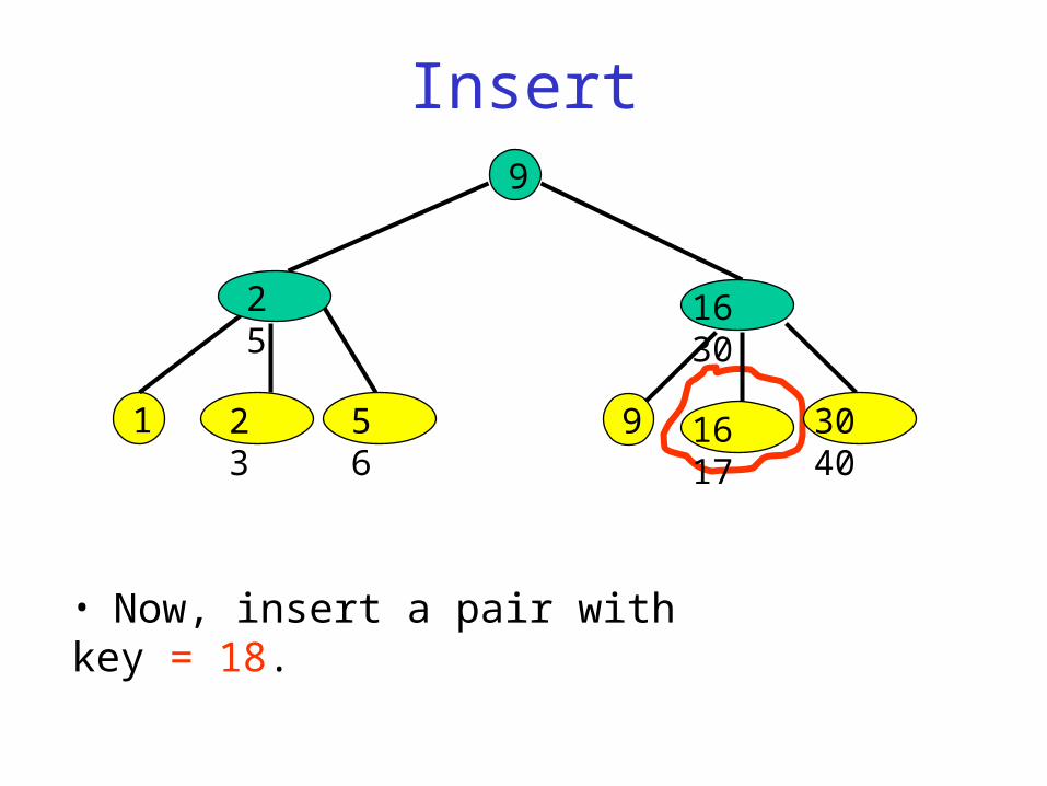
Insert
• Now, insert a pair with key = 18.
9
1
2 5
5 6 30 409 16 17
16 30
2 3
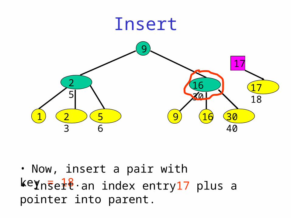
Insert
• Now, insert a pair with key = 18.
9
1
2 5
5 6 30 409
16 30
2 3 16
17
17 18
• Insert an index entry17 plus a pointer into parent.
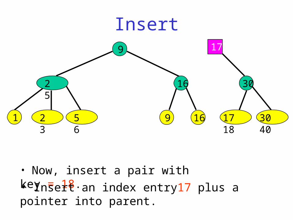
Insert
• Now, insert a pair with key = 18.
9
1
2 5
5 62 3
• Insert an index entry17 plus a pointer into parent.
9
16
16 17 18 30 40
17
30
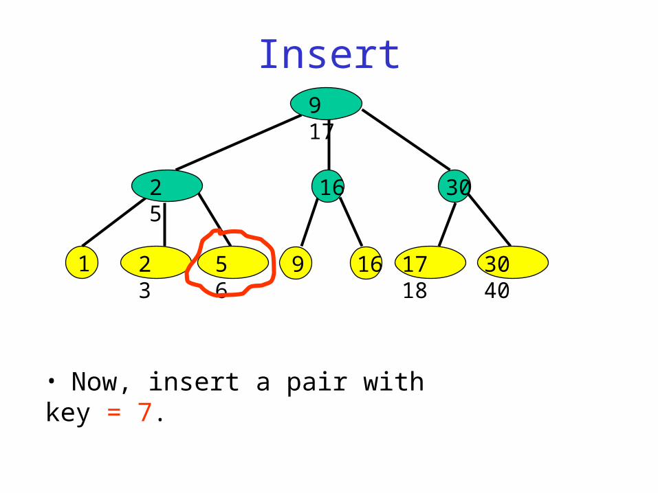
Insert
• Now, insert a pair with key = 7.
1
2 5
5 62 3 9
16
16 17 18 30 40
30
9 17
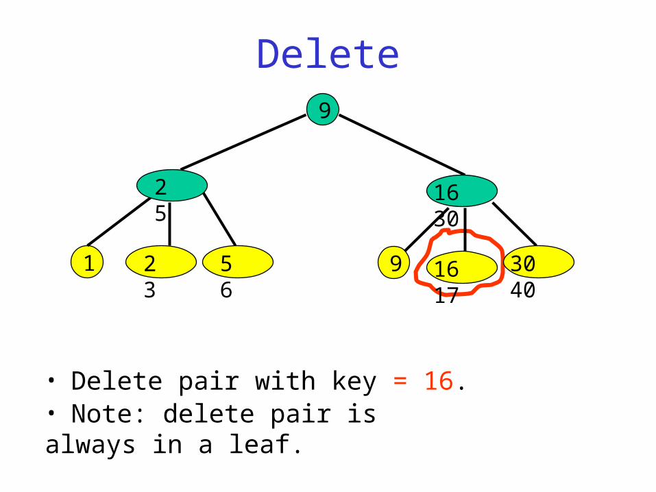
Delete
• Delete pair with key = 16.
9
1
2 5
5 6 30 409 16 17
16 30
2 3
• Note: delete pair is always in a leaf.
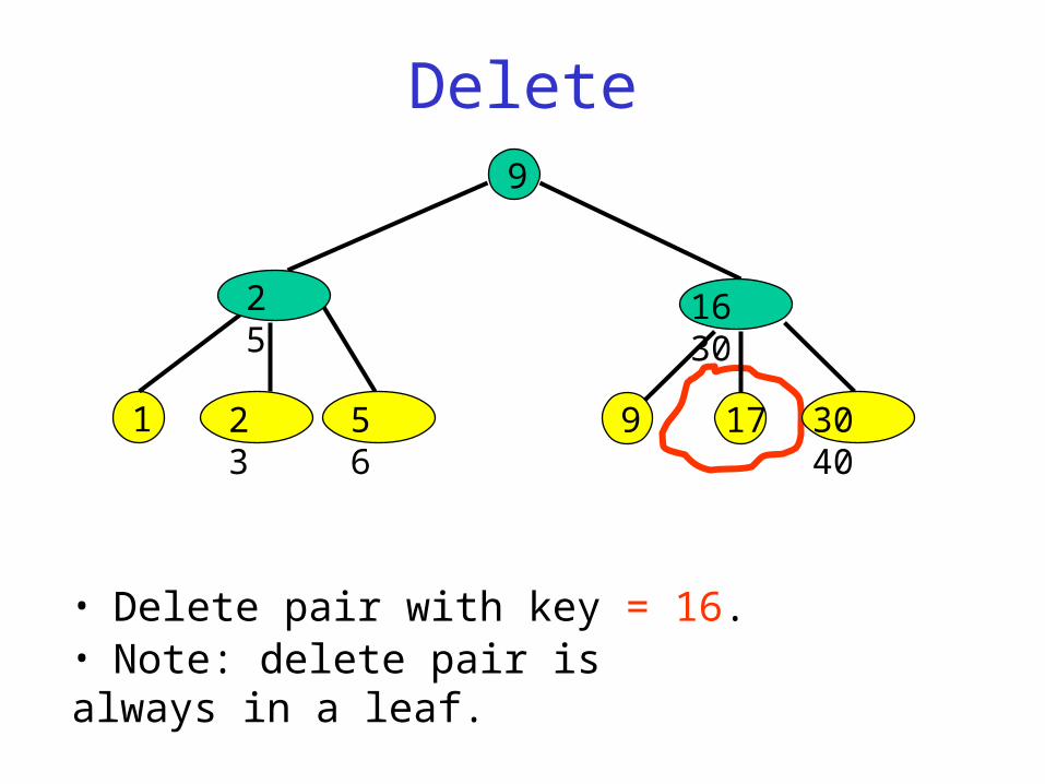
Delete
• Delete pair with key = 16.
9
1
2 5
5 6 30 409
16 30
2 3
• Note: delete pair is always in a leaf.
17
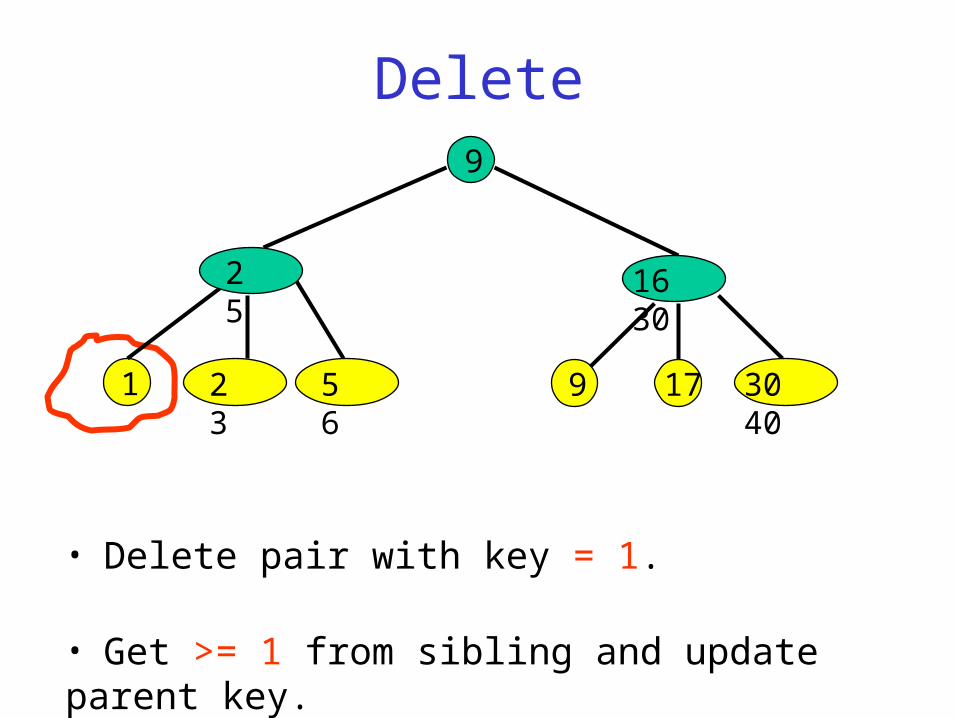
Delete
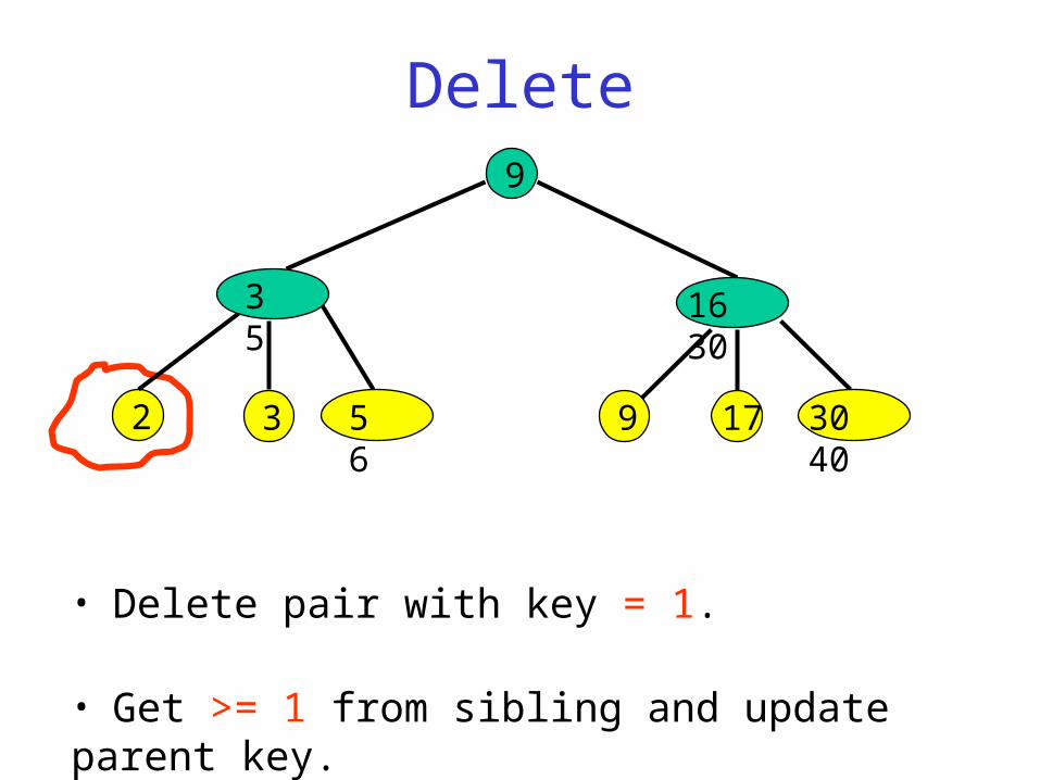
• Delete pair with key = 1.
9
1
2 5
5 6 30 409
16 30
2 3 17
• Get >= 1 from sibling and update parent key.
Delete
• Delete pair with key = 1.
9
2
3 5
5 6 30 409
16 30
17
• Get >= 1 from sibling and update parent key.
3
Delete
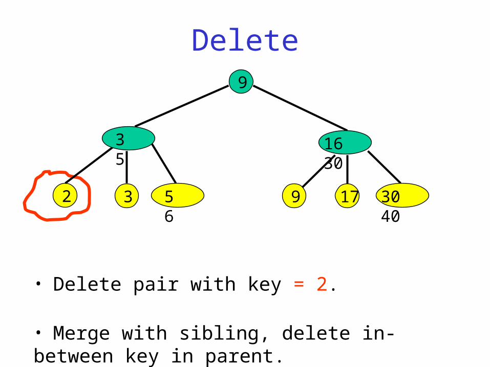
• Delete pair with key = 2.
9
2
3 5
5 6 30 409
16 30
17
• Merge with sibling, delete in-between key in parent.
3
Delete
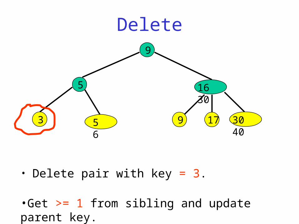
• Delete pair with key = 3.
9
3 5 6 30 409
16 30
17
•Get >= 1 from sibling and update parent key.
5
Delete
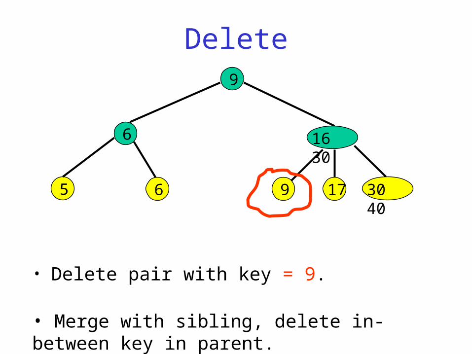
• Delete pair with key = 9.
9
5 30 409
16 30
17
• Merge with sibling, delete in-between key in parent.
6
6
Delete9
5 30 4017
6
6
30
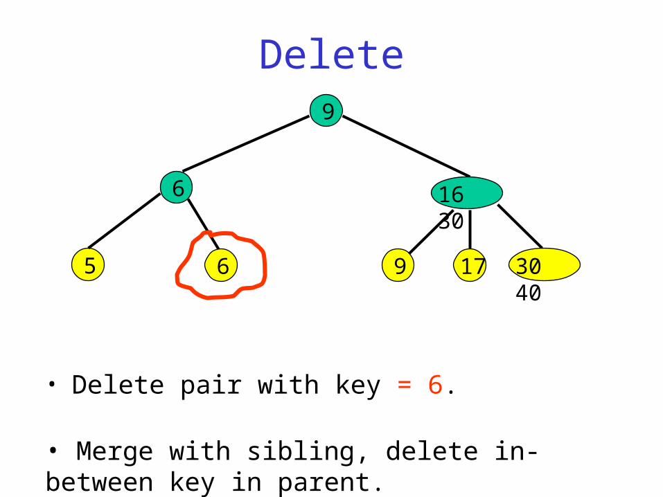
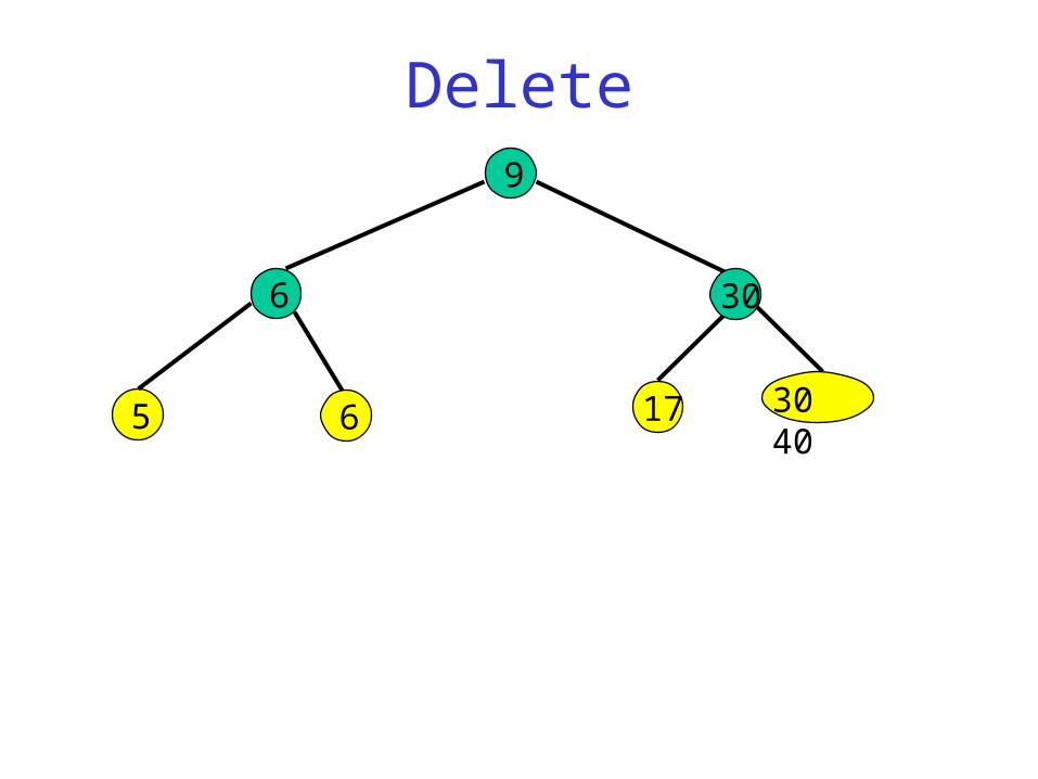
Delete
• Delete pair with key = 6.
9
5 30 409
16 30
17
• Merge with sibling, delete in-between key in parent.
6
6
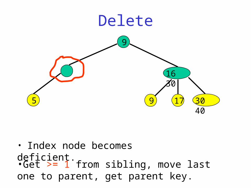
Delete
• Index node becomes deficient.
9
5 30 409
16 30
17
•Get >= 1 from sibling, move last one to parent, get parent key.
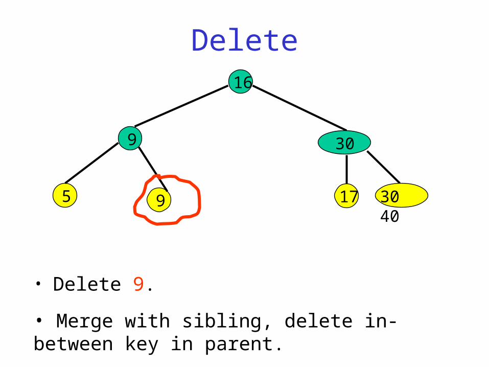
Delete
• Delete 9.
16
5 30 409
30
17
• Merge with sibling, delete in-between key in parent.
9
Delete
•Index node becomes deficient.
16
5 30 40
30
17
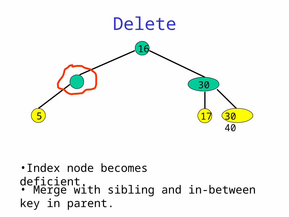
• Merge with sibling and in-between key in parent.
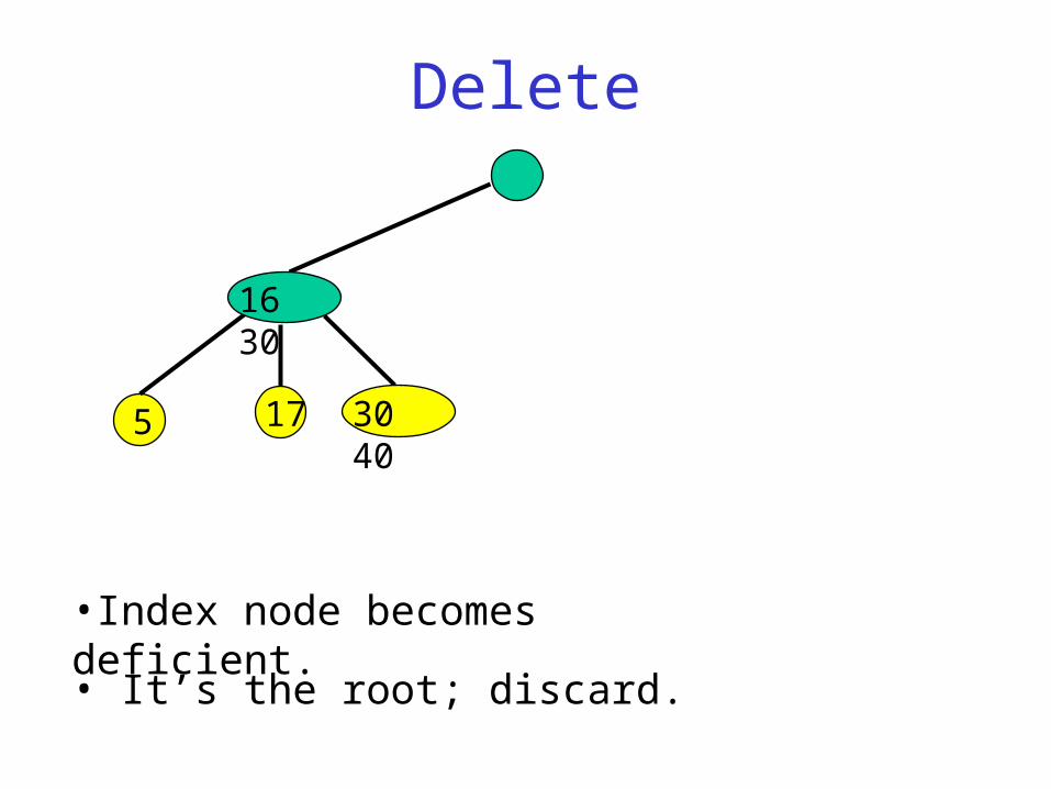
Delete
•Index node becomes deficient.
5 30 4017
• It’s the root; discard.
16 30
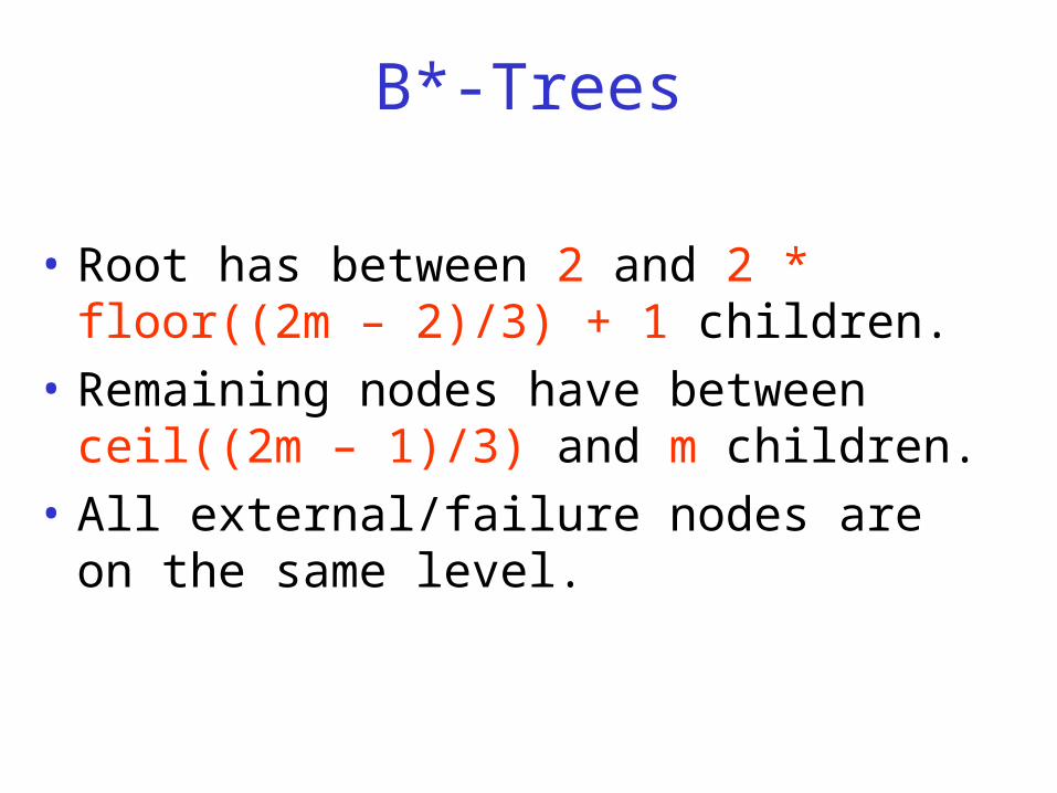
B*-Trees
• Root has between 2 and 2 * floor((2m – 2)/3) + 1 children.
• Remaining nodes have between ceil((2m – 1)/3) and m children.
• All external/failure nodes are on the same level.
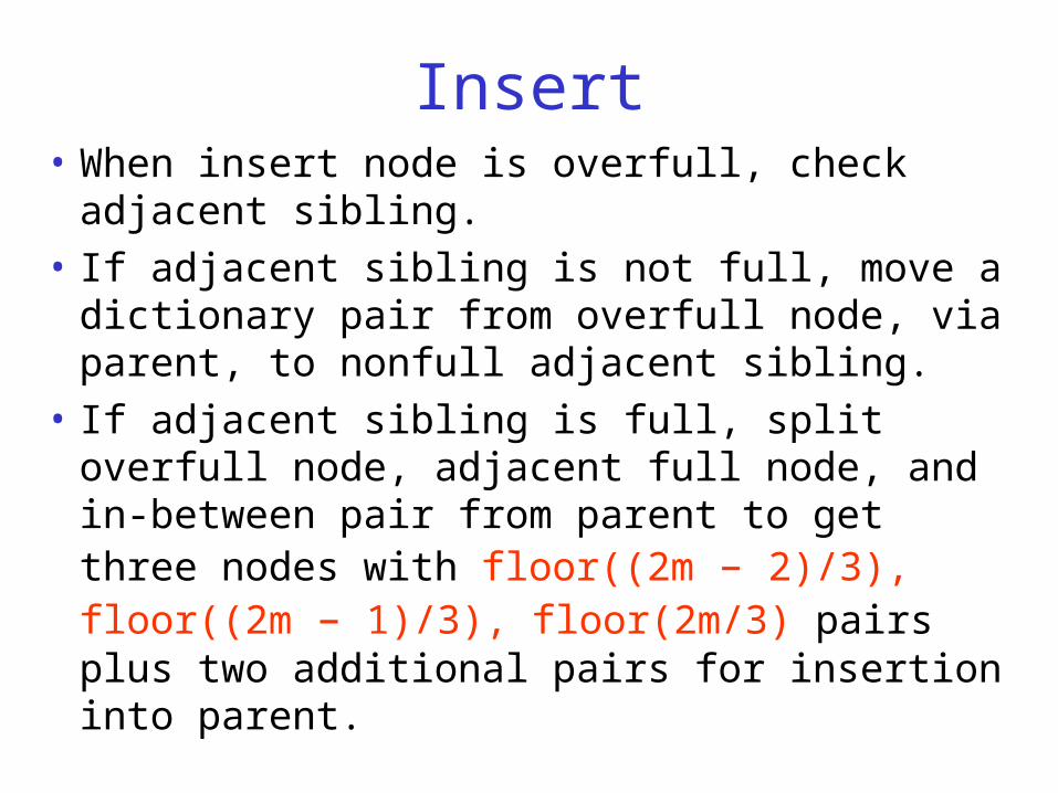
Insert• When insert node is overfull, check adjacent
sibling.
• If adjacent sibling is not full, move a dictionary pair from overfull node, via parent, to nonfull adjacent sibling.
• If adjacent sibling is full, split overfull node, adjacent full node, and in-between pair from parent to get three nodes with floor((2m – 2)/3), floor((2m – 1)/3), floor(2m/3) pairs plus two additional pairs for insertion into parent.
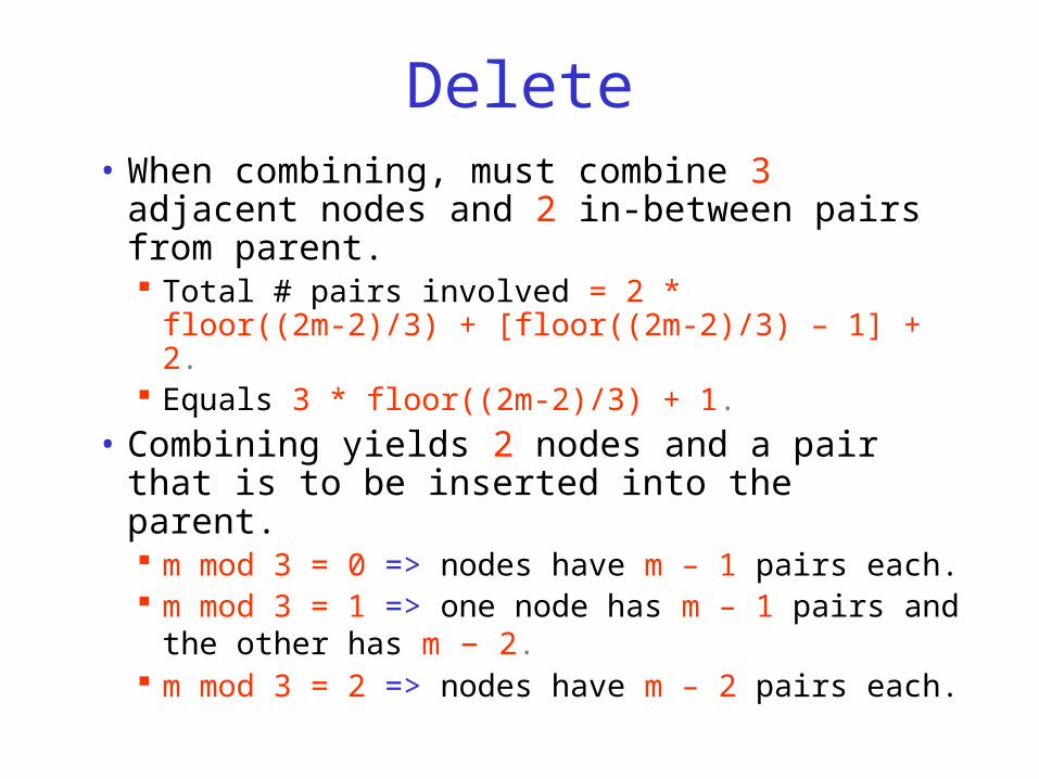
Delete• When combining, must combine 3 adjacent
nodes and 2 in-between pairs from parent. Total # pairs involved = 2 * floor((2m-2)/3) +
[floor((2m-2)/3) – 1] + 2. Equals 3 * floor((2m-2)/3) + 1.
• Combining yields 2 nodes and a pair that is to be inserted into the parent. m mod 3 = 0 => nodes have m – 1 pairs each. m mod 3 = 1 => one node has m – 1 pairs and
the other has m – 2. m mod 3 = 2 => nodes have m – 2 pairs each.
Splay Trees• Binary search trees.• Search, insert, delete, and split have amortized
complexity O(log n) & actual complexity O(n).• Actual and amortized complexity of join is O(1).• Priority queue and double-ended priority queue
versions outperform heaps, deaps, etc. over a sequence of operations.
• Two varieties. Bottom up. Top down.
Bottom-Up Splay Trees• Search, insert, delete, and join are done as in an
unbalanced binary search tree.
• Search, insert, and delete are followed by a splay operation that begins at a splay node.
• When the splay operation completes, the splay node has become the tree root.
• Join requires no splay (or, a null splay is done).
• For the split operation, the splay is done in the middle (rather than end) of the operation.
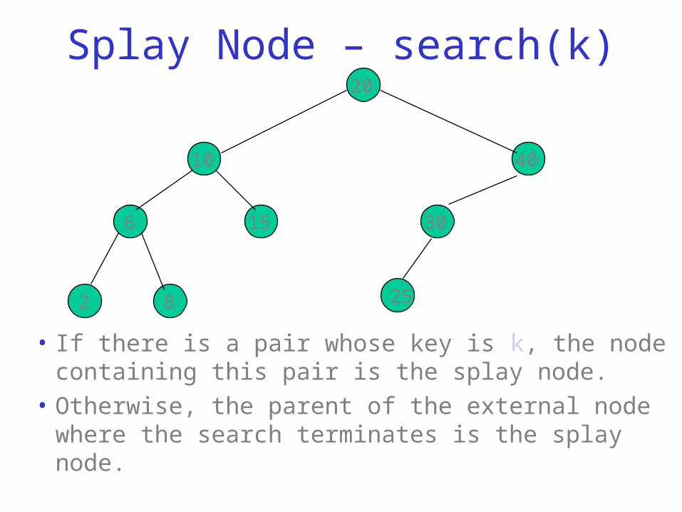
Splay Node – search(k)
• If there is a pair whose key is k, the node containing this pair is the splay node.
• Otherwise, the parent of the external node where the search terminates is the splay node.
20
10
6
2 8
15
40
30
25
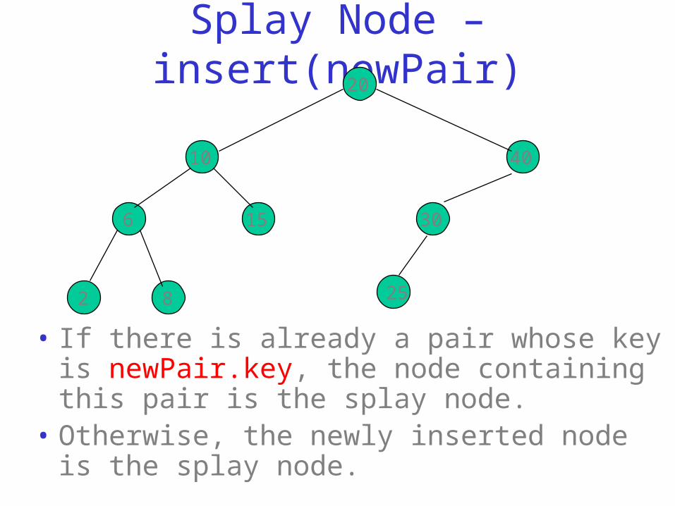
Splay Node – insert(newPair)
• If there is already a pair whose key is newPair.key, the node containing this pair is the splay node.
• Otherwise, the newly inserted node is the splay node.
20
10
6
2 8
15
40
30
25
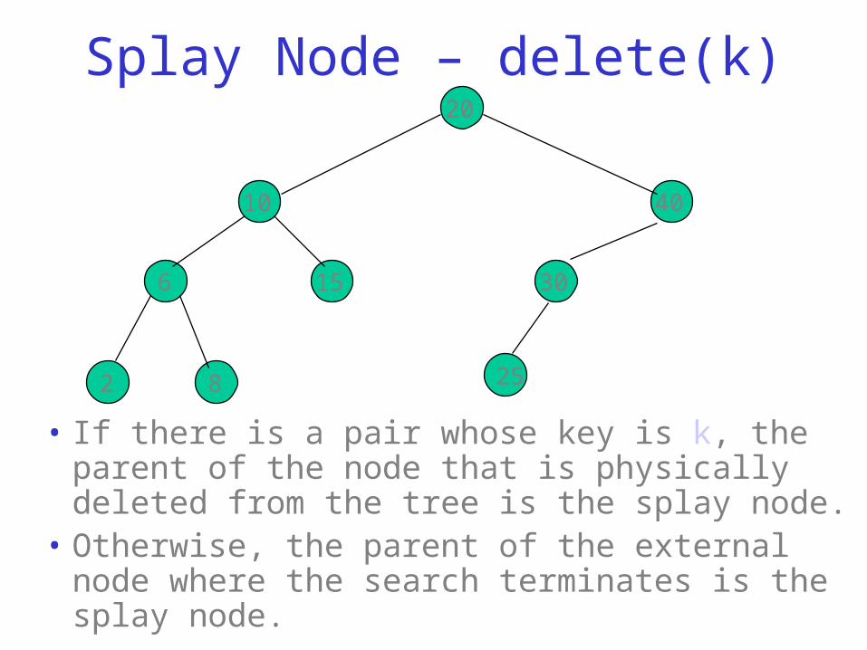
Splay Node – delete(k)
• If there is a pair whose key is k, the parent of the node that is physically deleted from the tree is the splay node.
• Otherwise, the parent of the external node where the search terminates is the splay node.
20
10
6
2 8
15
40
30
25
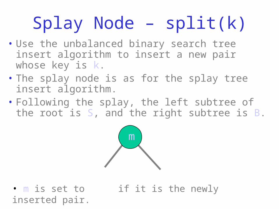
Splay Node – split(k)• Use the unbalanced binary search tree insert
algorithm to insert a new pair whose key is k. • The splay node is as for the splay tree insert
algorithm.• Following the splay, the left subtree of the root is
S, and the right subtree is B.
S
m
B• m is set to null if it is the newly inserted pair.
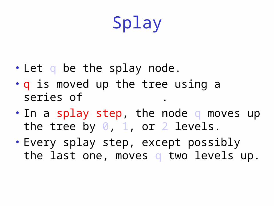
Splay
• Let q be the splay node.
• q is moved up the tree using a series of splay steps.
• In a splay step, the node q moves up the tree by 0, 1, or 2 levels.
• Every splay step, except possibly the last one, moves q two levels up.
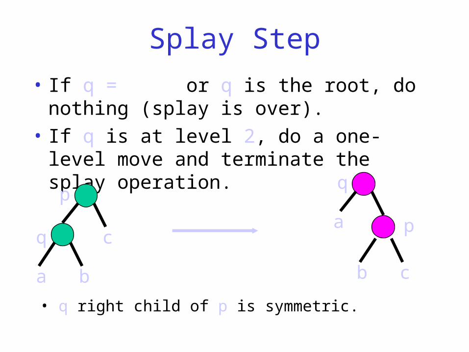
Splay Step
• If q = null or q is the root, do nothing (splay is over).
• If q is at level 2, do a one-level move and terminate the splay operation.
p
q
a b
c
b c
a
q
p
• q right child of p is symmetric.
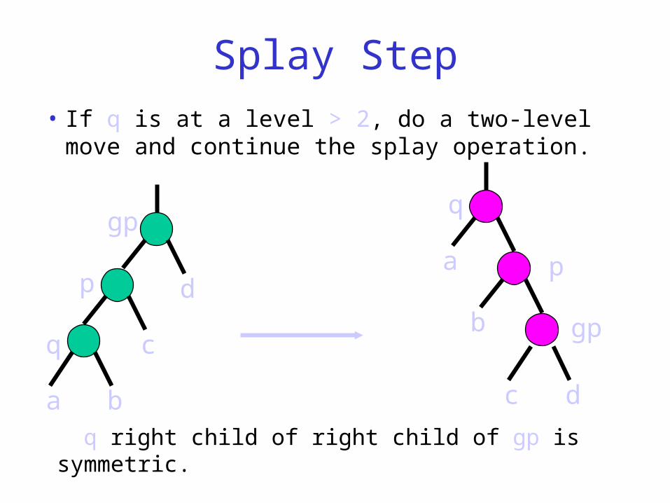
Splay Step
• If q is at a level > 2, do a two-level move and continue the splay operation.
• q right child of right child of gp is symmetric.
p
q
a b
c
gp
d
c d
b
p
gp
q
a
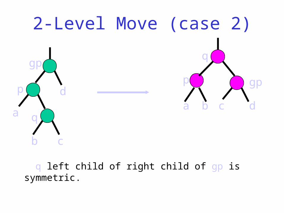
2-Level Move (case 2)
• q left child of right child of gp is symmetric.
p
q
b c
a
gp
da cb
gpp
q
d
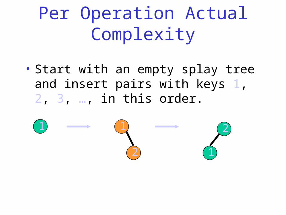
Per Operation Actual Complexity
• Start with an empty splay tree and insert pairs with keys 1, 2, 3, …, in this order.
1 1
2 1
2
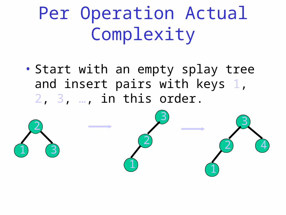
Per Operation Actual Complexity
• Start with an empty splay tree and insert pairs with keys 1, 2, 3, …, in this order.
1
2
31
2
3
1
2
3
4
Per Operation Actual Complexity
• Worst-case height = n.• Actual complexity of search, insert, delete,
and split is O(n).
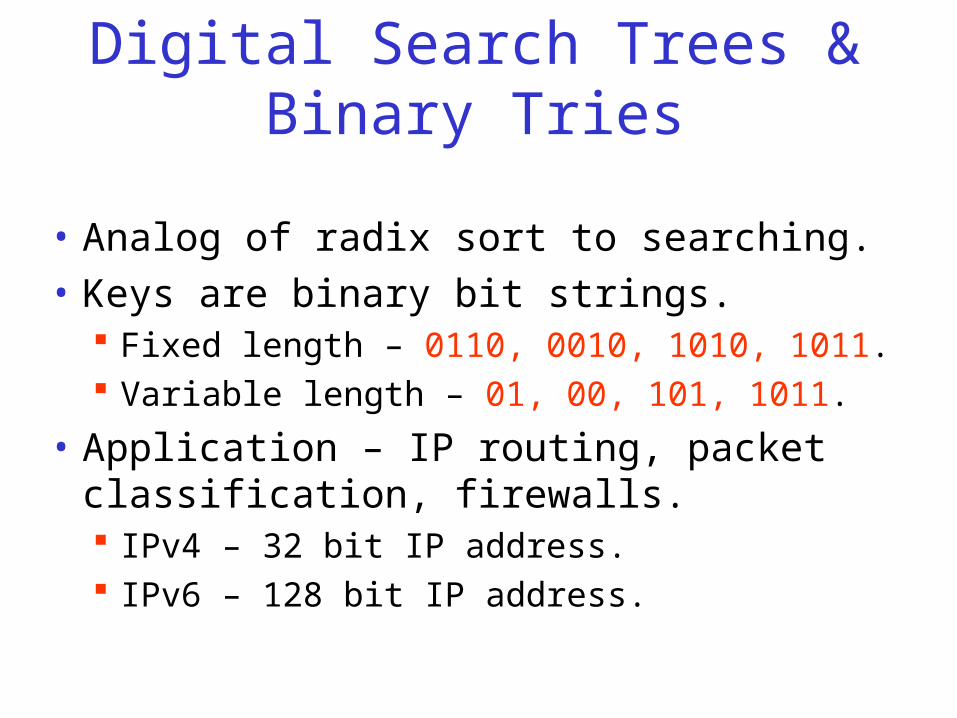
Digital Search Trees & Binary Tries
• Analog of radix sort to searching.
• Keys are binary bit strings. Fixed length – 0110, 0010, 1010, 1011. Variable length – 01, 00, 101, 1011.
• Application – IP routing, packet classification, firewalls. IPv4 – 32 bit IP address. IPv6 – 128 bit IP address.
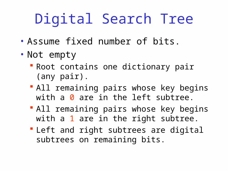
Digital Search Tree
• Assume fixed number of bits.
• Not empty => Root contains one dictionary pair (any pair). All remaining pairs whose key begins with a 0
are in the left subtree. All remaining pairs whose key begins with a 1
are in the right subtree. Left and right subtrees are digital subtrees on
remaining bits.
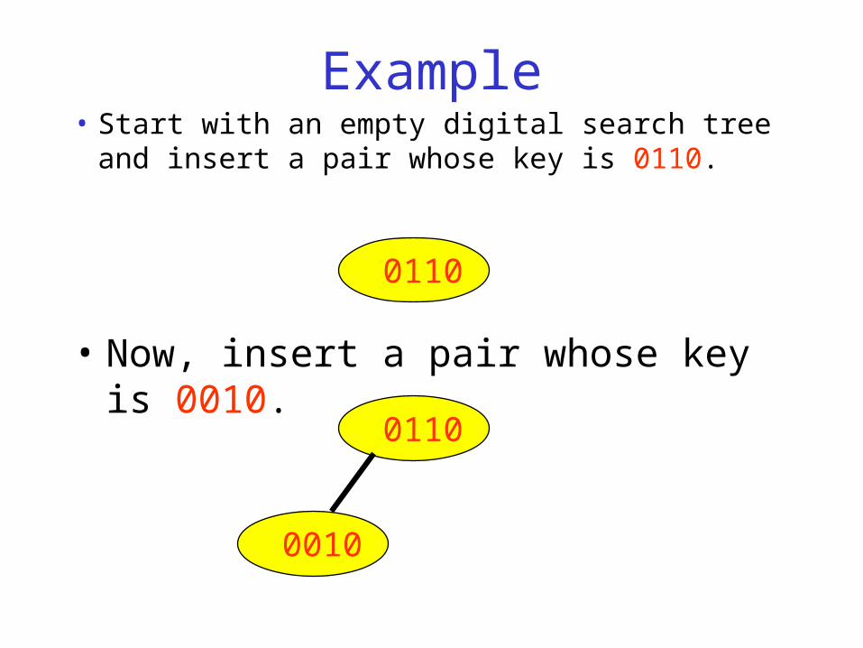
Example• Start with an empty digital search tree and
insert a pair whose key is 0110.
0110
• Now, insert a pair whose key is 0010.
0110
0010
Example
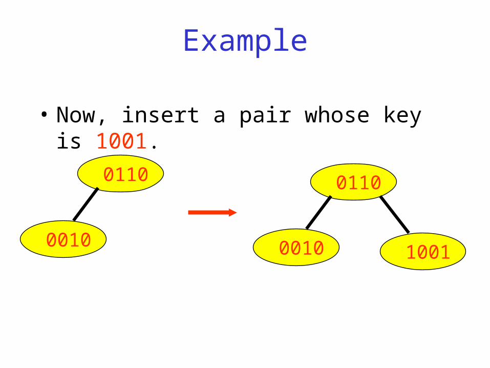
• Now, insert a pair whose key is 1001.
0110
00101001
0110
0010
Example
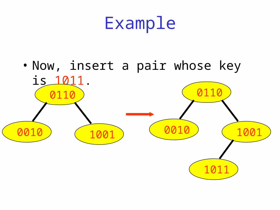
• Now, insert a pair whose key is 1011.
1001
0110
0010 1001
0110
0010
1011
Example
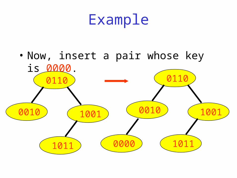
• Now, insert a pair whose key is 0000.
1001
0110
0010
1011
1001
0110
0010
10110000
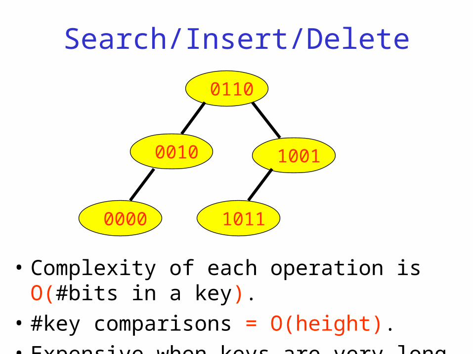
Search/Insert/Delete
• Complexity of each operation is O(#bits in a key).
• #key comparisons = O(height).
• Expensive when keys are very long.
1001
0110
0010
10110000
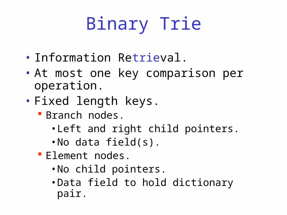
Binary Trie
• Information Retrieval.• At most one key comparison per operation.• Fixed length keys.
Branch nodes.• Left and right child pointers.• No data field(s).
Element nodes.• No child pointers.• Data field to hold dictionary pair.
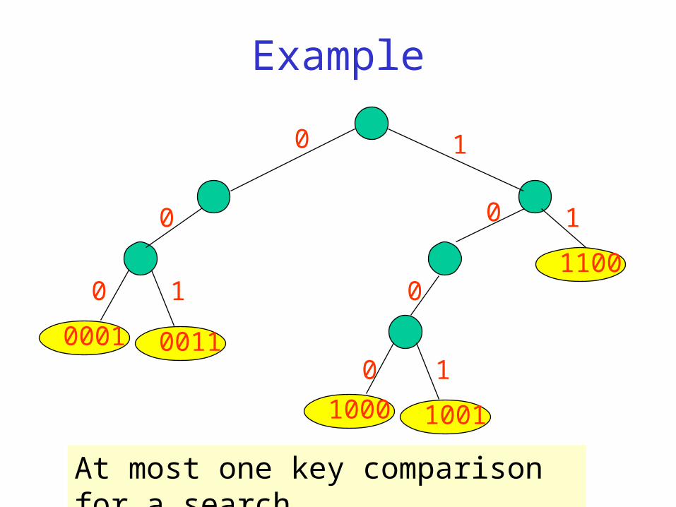
Example
At most one key comparison for a search.
0001 0011
1100
1000 1001
0
0
0
0
0
0
1
1
1
1
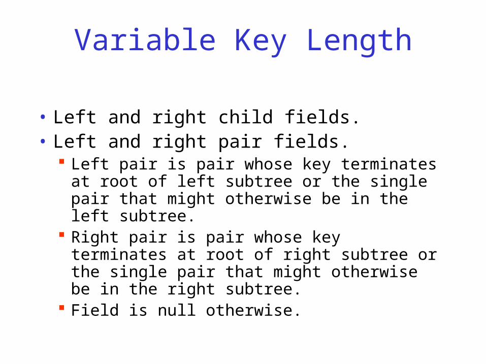
Variable Key Length
• Left and right child fields.• Left and right pair fields.
Left pair is pair whose key terminates at root of left subtree or the single pair that might otherwise be in the left subtree.
Right pair is pair whose key terminates at root of right subtree or the single pair that might otherwise be in the right subtree.
Field is null otherwise.
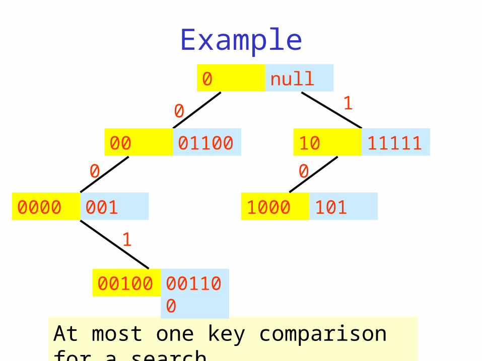
Example
At most one key comparison for a search.
0 10 null
00 01100
0000 001
10 11111
00100 001100
1000 101
0 0
1
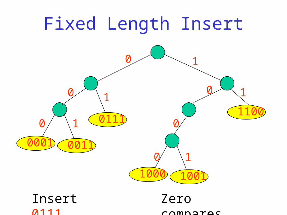
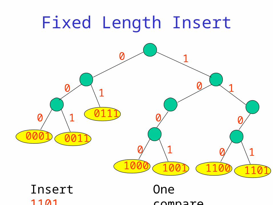
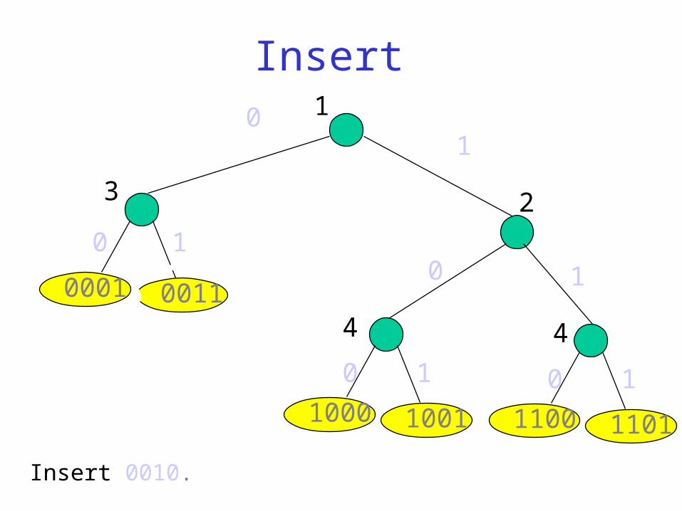
Fixed Length Insert
Insert 0111.
0001 0011
1100
1000 1001
0
0
0
0
0
0
1
1
1
1 0111
1
Zero compares.
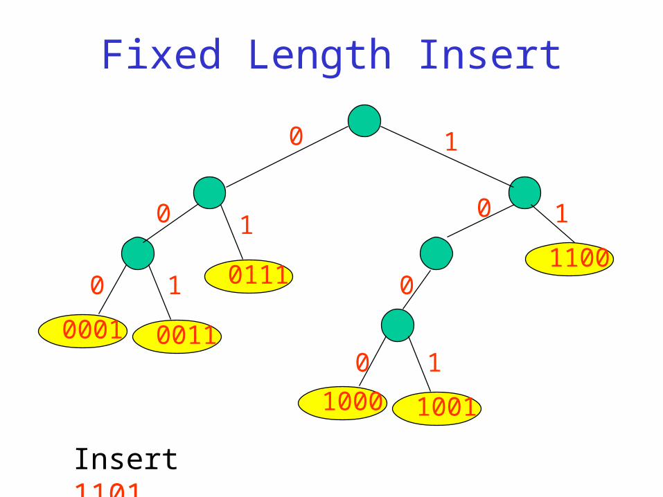
Fixed Length Insert
Insert 1101.
0001 0011
1100
1000 1001
0
0
0
0
0
0
1
1
1
1 0111
1
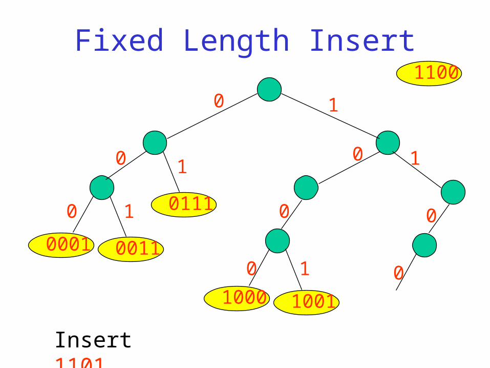
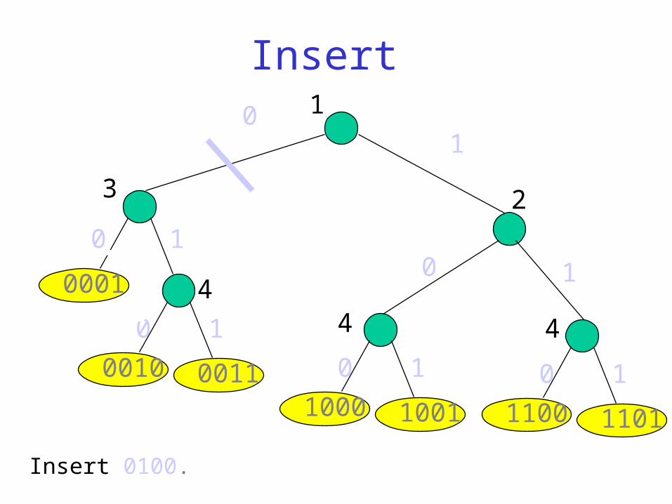
Fixed Length Insert
Insert 1101.
1100
0 1
0001 0011
1000 1001
0
0
0
0
0
1
1
1 0111
1
0
0
Fixed Length Insert
Insert 1101.
0 1
0001 0011
1000 1001
0
0
0
0
0
1
1
1 0111
1
One compare.
1100 1101
0
0
1
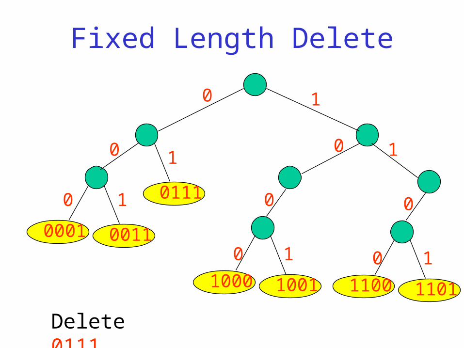
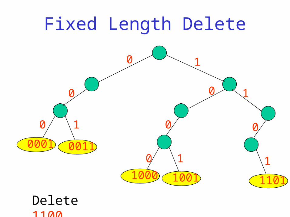
Fixed Length Delete
Delete 0111.
0 1
0001 0011
1000 1001
0
0
0
0
0
1
1
1 0111
1
1100 1101
0
0
1
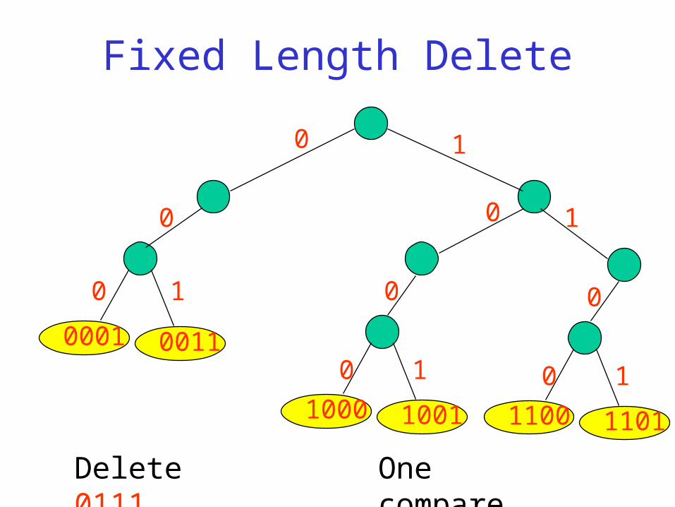
Fixed Length Delete
Delete 0111. One compare.
0 1
0001 0011
1000 1001
0
0
0
0
0
1
1
1
1100 1101
0
0
1
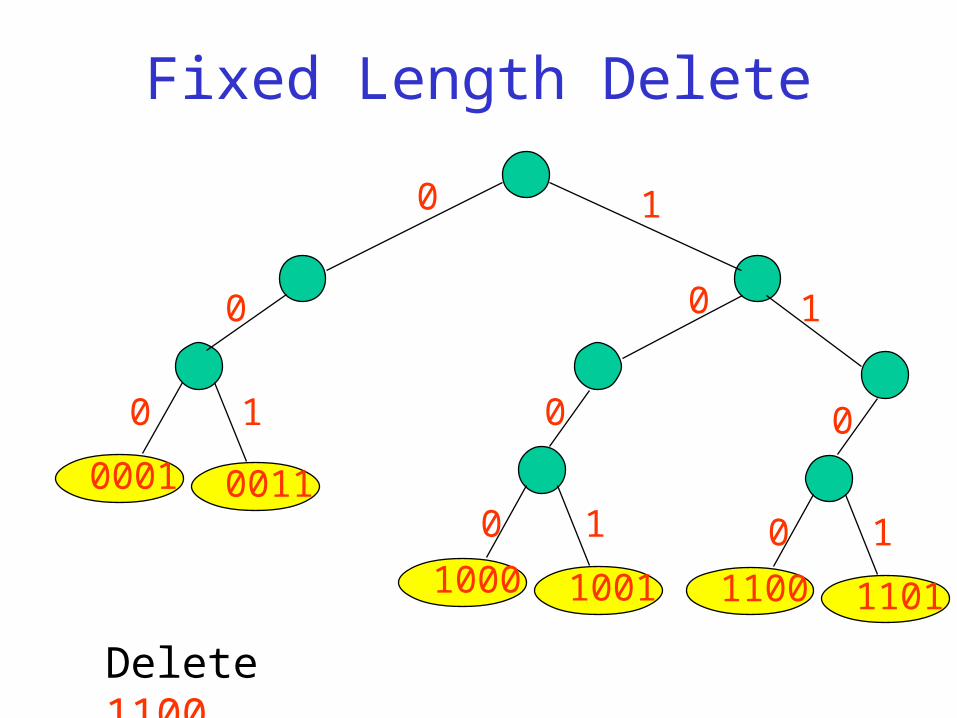
Fixed Length Delete
Delete 1100.
0 1
0001 0011
1000 1001
0
0
0
0
0
1
1
1
1100 1101
0
0
1
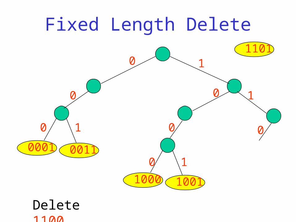
Fixed Length Delete
Delete 1100.
0 1
0001 0011
1000 1001
0
0
0
0
0
1
1
1
1101
0
1
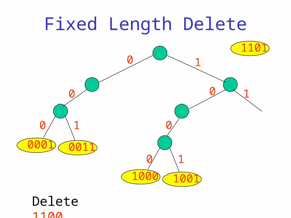
Fixed Length Delete
Delete 1100.
0 1
0001 0011
1000 1001
0
0
0
0
0
1
1
1
1101
0
Fixed Length Delete
Delete 1100.
0 1
0001 0011
1000 1001
0
0
0
0
0
1
1
1
1101
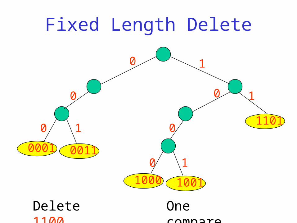
Fixed Length Delete
Delete 1100. One compare.
0 1
0001 0011
1000 1001
0
0
0
0
0
1
1
11101
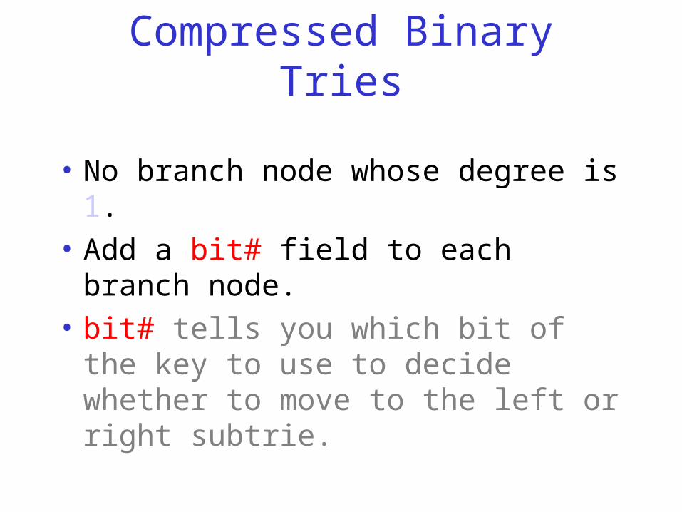
Compressed Binary Tries
• No branch node whose degree is 1.
• Add a bit# field to each branch node.
• bit# tells you which bit of the key to use to decide whether to move to the left or right subtrie.
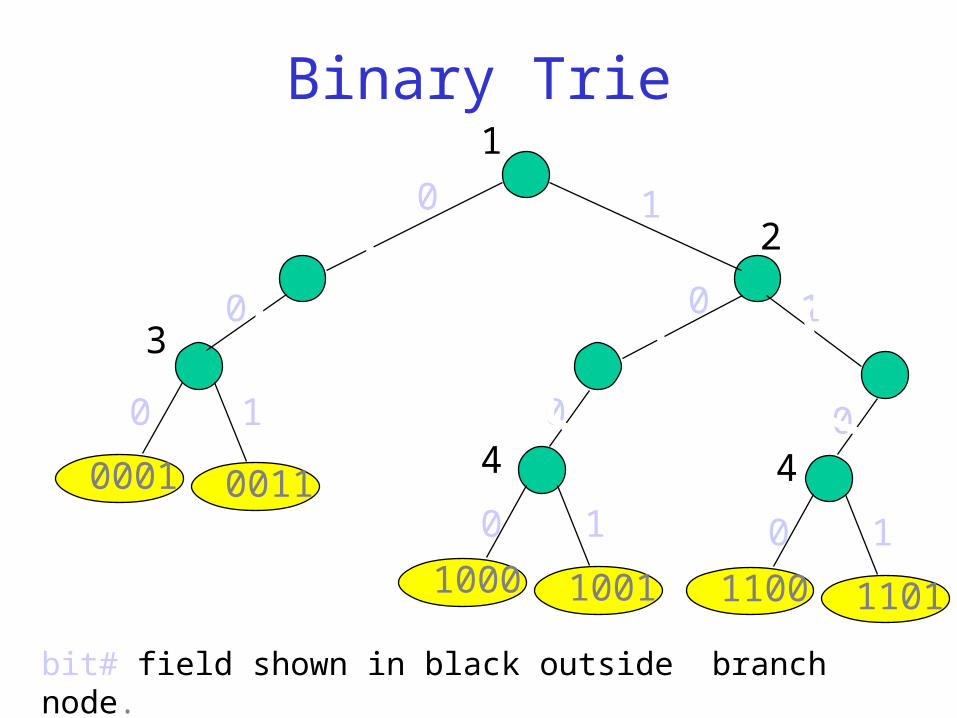
Binary Trie
0 1
0001 0011
1000 1001
0
0
0
0
0
1
1
1
1100 1101
0
0
1
1
2
3
4 4
bit# field shown in black outside branch node.
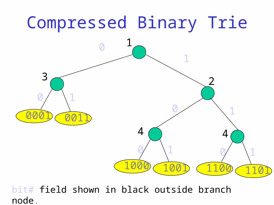
Compressed Binary Trie
0 10001 0011
1000 1001
0
0
0
1
1
1
1100 1101
0 1
1
23
4 4
bit# field shown in black outside branch node.
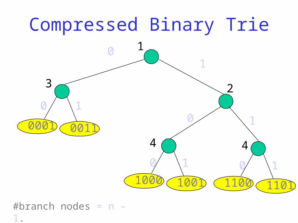
Compressed Binary Trie
0 10001 0011
1000 1001
0
0
0
1
1
1
1100 1101
0 1
1
23
4 4
#branch nodes = n – 1.
Insert
0 10001 0011
1000 1001
0
0
0
1
1
1
1100 1101
0 1
1
23
4 4
Insert 0010.
Insert
Insert 0100.
0 10001
1000 1001
0
0
0
1
1
1
1100 1101
0 1
1
23
4 4
0010 0011
0 1
4
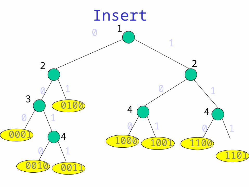
Insert
0 1
00011000 1001
0
00
1
11
11001101
0 1
1
2
34 4
0010 0011
0 1
4
2
0
0100
1
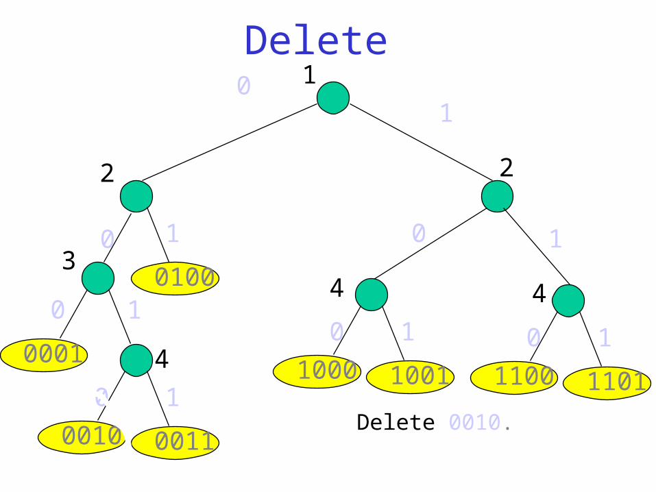
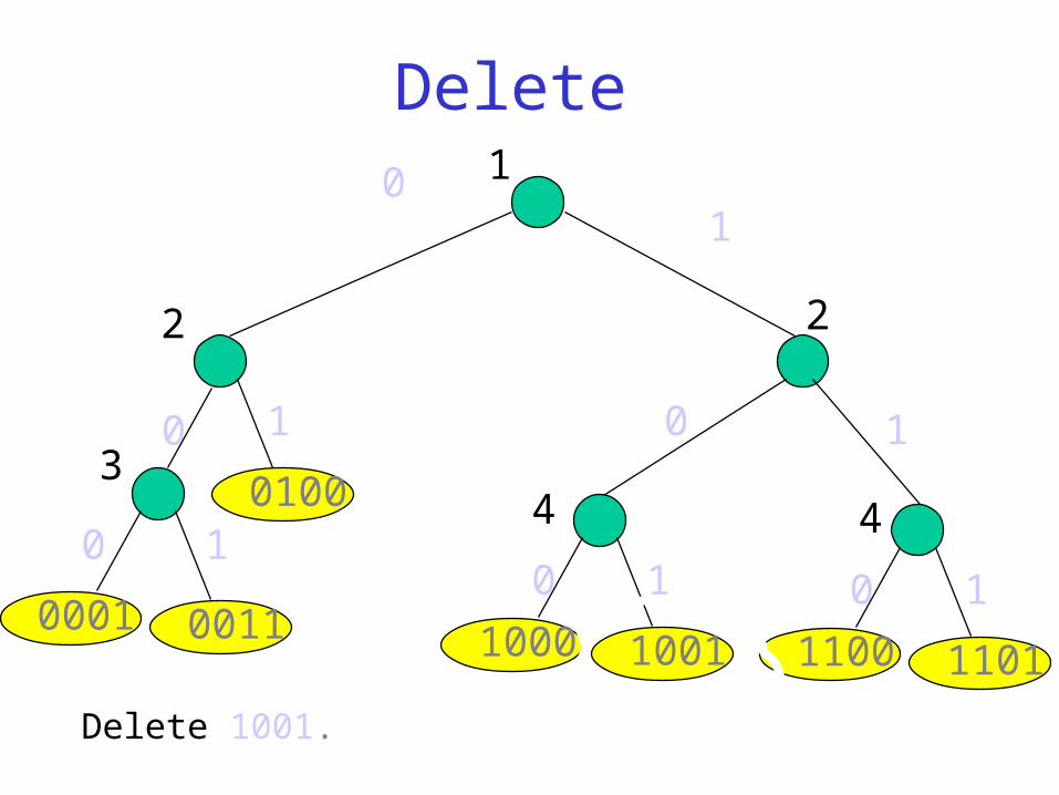
Delete
0001
0 1
1000 1001
0
00
1
11
1100 1101
0 1
1
2
34 4
0010 0011
0 1
4
2
0
0100
1
Delete 0010.
Delete
0001
0 1
1000 1001
0
00
1
11
1100 1101
0 1
1
2
34 4
0011
2
0
0100
1
Delete 1001.
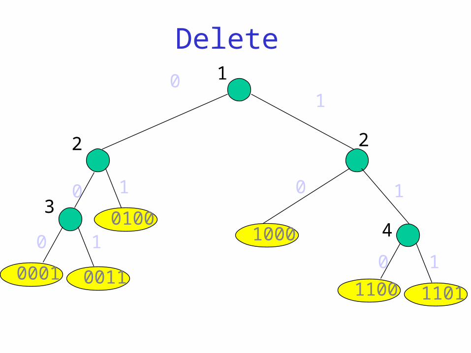
Delete
0001
0 1
1000
0
0
1
1
1100 1101
0 1
1
2
34
0011
2
0
0100
1