Bachelor in Mathematics

Experimental Mathematics 4

Winter semester 2020/21

Solving polynomial equations

Authors:

Clara Popescu

Dylan Mota

Kim Da Cruz

Supervisors:

Prof. Dr. Gabor Wiese

Guendalina Palmirotta

Abstract

In the following, we will take a look at some methods to factorise polyno-

mials. More precisely, we will study the Newton-Raphson method for solving

polynomial equations over real numbers and for factorisation over �nite �elds,

we will look at Berlekamp's algorithm. Moreover, we will examine Hensel's

Lemma in order to solve polynomial equations modulo pn, where n ∈ N and

p is a prime number. Our goal is to become familiar with methods used for

solving polynomial equations over real numbers and over �nite �elds.

1

Contents

1 Introduction 31.1 Quadratic equations . . . . . . . . . . . . . . . . . . . . . . . . . . . 31.2 Cubic equations . . . . . . . . . . . . . . . . . . . . . . . . . . . . . . 5

2 Solving polynomial equations over real numbers using Newton'sapproximation 72.1 Newton-Raphson method . . . . . . . . . . . . . . . . . . . . . . . . . 8

2.1.1 Explanation of the method . . . . . . . . . . . . . . . . . . . . 82.1.2 Problems of the Newton-Raphson method . . . . . . . . . . . 92.1.3 Geometric illustration . . . . . . . . . . . . . . . . . . . . . . 112.1.4 Algorithmic illustration . . . . . . . . . . . . . . . . . . . . . . 13

2.2 Revisited Newton-Raphson method with faster convergence . . . . . . 182.2.1 Explanation of the method . . . . . . . . . . . . . . . . . . . . 182.2.2 Geometric illustration . . . . . . . . . . . . . . . . . . . . . . 212.2.3 Algorithmic illustration . . . . . . . . . . . . . . . . . . . . . . 23

3 Factorising polynomials over �nite �elds using Berlekamp's algo-rithm 293.1 General statement . . . . . . . . . . . . . . . . . . . . . . . . . . . . 293.2 Algorithmic illustration . . . . . . . . . . . . . . . . . . . . . . . . . . 32

4 Solving polynomial congruence equations using Hensel's Lemma 404.1 General statement . . . . . . . . . . . . . . . . . . . . . . . . . . . . 404.2 Algorithmic illustration . . . . . . . . . . . . . . . . . . . . . . . . . . 42

5 Conclusion 49

6 References 51

2

1 Introduction

Factorisation of polynomials, or solving polynomial equations sounds easy when weare talking about real polynomials of small degrees. In these cases, there exist somewell-known formulas that are easily applicable. Let us start with the easiest case,where the polynomial has degree 2.

1.1 Quadratic equations

First, let us recall that a quadratic equation is an equation that can be rearrangedto the point that it is of the form:

ax2 + bx+ c = 0, (1)

where x ∈ R is the unknown variable, a, b, c ∈ R are the known coe�cients suchthat a 6= 0, otherwise we would have a linear equation.In order to solve such an equation, one can use a few methods. One way is to �rstfactorise it using the standard algebraic identities:

ab+ ac = a(b+ c)

ac+ ad+ bc+ bd = (a+ b)(c+ d)

a2 + 2ab+ b2 = (a+ b)2

a2 − 2ab+ b2 = (a− b)2

a2 − b2 = (a+ b)(a− b).After applying these to the polynomial in the equation, we use the "zero factorproperty" that states that if ab = 0, then a = 0 or b = 0.Another method is the process of completing the square. Here, we try to use thealgebraic identity

a2 + 2ab+ b2 = (a+ b)2. (2)

Consider the quadratic equation (1) from above, in order to use (2), we do thefollowing calculations:

ax2 + bx+ c = 0 | : a

x2 +b

ax+

c

a= 0 | − c

a

x2 +b

ax = − c

a|+(b

2a

)2

x2 +b

ax+

(b

2a

)2

= − ca

+

(b

2a

)2

| use identity (2) on the lefthand side(x+

b

2a

)2

=b2 − 4ac

4a2.

3

Finally, we solve the equation by taking the square root and subtracting b2a

on bothsides: (

x+b

2a

)2

=b2 − 4ac

4a2| take the square root

x+b

2a= ±

√b2 − 4ac

4a2| − b

2a

x = ±√b2 − 4ac

2a− b

2a.

Completing the square can be used to derive a general formula for solving quadraticequations, called the quadratic formula. Given the quadratic equation (1), thequadratic formula is given by:

x =−b±

√b2 − 4ac

2a=−b±

√∆

2a.

where, the expression under the square root is called the discriminant and is denotedby the greek letter ∆. In fact, the discriminant determines the number of real rootsthe quadratic equation has:

� If ∆ > 0, then the equation has 2 real roots given by:

x =−b+

√∆

2aand x =

−b−√

∆

2a,

� If ∆ = 0, then the equation has one real root given by:

x =−b2a,

� If ∆ < 0, then the equation has no real roots, since we would take the squareroot of a negative number in the quadratic formula. In this case, we have 2complex roots.

We can conclude that there are a lot of methods for solving these equations. Afterhaving looked at equations of degree 2, we are going to look at methods for solvingpolynomial equations of degree 3.

4

1.2 Cubic equations

Let us recall that a cubic equation is an equation that it is of the form:

ax3 + bx2 + cx+ d = 0, (3)

where x ∈ R is again the unknown variable, a, b, c, d ∈ R are the known coe�cientssuch that a 6= 0, otherwise we would speak of a quadratic equation.As for the quadratic equations, there is more than one method for solving cubicequations, one of them being factoring out common factors, or factorisation usingthe standard algebraic identities:

a3 + 3a2b+ 3ab2 + b3 = (a+ b)3

a3 − 3a2b+ 3ab2 − b3 = (a− b)3

a3 − b3 = (a− b)(a2 + ab+ b2)

a3 + b3 = (a+ b)(a2 − ab+ b2).

After applying these to the polynomial of the equation, we use again the "zero factorproperty" and if necessary, we have to solve a quadratic equation using one of themethods stated in the previous subsection.In order to look at another method, let us recall the meaning of a depressed cubic.A depressed cubic is a polynomial of degree 3 of the form:

t3 + pt+ q,

where t is a real variable and p, q are real coe�cients. This type of cubic polynomialis much simpler to study, however it's still fundamental since any cubic can bereduced to a depressed cubic by a change of variable. In fact, consider the generalcubic equation (3). If we set x := t − b

3aand calculate everything out, then we

obtain:

at3 + t

(3ac− b2

3a

)+

2b3 − 9abc+ 27a2d

27a2.

Thus, by dividing by a, we obtain the depressed cubic equation:

t3 + pt+ q = 0, (4)

where t = x+ b3a, p = 3ac−b2

3a2and q = 2b3−9abc+27a2d

27a3.

The next method we are going to explain is Cardano's formula. This formula onlysolves depressed cubic equations, however, as stated above, any cubic polynomialcan be reduced to a depressed cubic. Consider the depressed equation (4), thenCardano states that the solutions are given by:

tk = uk + vk,

5

with k ∈ {0, 1, 2} and

uk = ξk 3

√√√√1

2

(−q +

√−∆

27

), vk = ξ−k 3

√√√√1

2

(−q −

√−∆

27

),

where ∆ = −(4p3+27q2) is the discriminant of the depressed cubic and ξ = −1+√−3

2.

There are 3 possible cases:

� If ∆ > 0, then there are three real solutions.

� If ∆ = 0, then there are either two real roots, such that one of them hasmultiplicity 2 and the other root has multiplicity 1, or there is one real solutionof multiplicity 3.

� If ∆ < 0, then there is one real solution and 2 complex solutions that arecomplex conjugates.

For more information, we refer to [3].From Cardano's formula, we can deduce a general cubic formula. Consider theequation (3) and set:

∆0 = b2 − 3ac

∆1 = 2b3 − 9abc+ 27a2d

C =3

√∆1 ±

√∆2

1 − 4∆30

2.

Then one of the roots of the equation is given by:

x = − 1

3a

(b+ C +

∆0

C

).

The other two roots can be found, either by changing the choice of the cube rootor by multiplying C by a primitive cube root of unity, that is −1±

√−3

2. So the three

roots are given by:

xk = − 1

3a

(b+ ξkC +

∆0

ξkC

),

where k ∈ {0, 1, 2} and ξ = −1+√−3

2.

We have already seen that polynomial equations of degree 3 are more di�cult tosolve than polynomial equations of degree 2. Next, we are going to study a methodfor solving polynomial equations of higher degrees. This method does not only workfor polynomial equations, but also for non-linear equations.

6

2 Solving polynomial equations over real numbers

using Newton's approximation

In this section, we are going to explain one of the fundamental problems in numericalanalysis, which is solving non-linear equations. Consider, for example, the followingequation:

e−x = x, x ∈ R.

It can be represented graphically:

Figure 1: Graphic representation of e−x = x, for x ∈ R.

We can observe that the curves of y = e−x (in green) and y = x (in red) onlyintersect in one point in the interval ]0, 1[, thus the equation e−x = x has a uniquesolution in ]0, 1[. However, it is nearly impossible to �nd this solution analytically.To solve equations of this type, where no solution can be found analytically, one of-ten uses iterative methods. That is, we start with an initial "guess" of the solutionand correct it using an algorithm that hopefully makes the initial "guess" convergeto the "correct solution".

7

One of these methods is the so-called Newton-Raphson method. The idea behindthe Newton-Raphson method is to approximate the root of a function that is con-tinuous and di�erentiable by tangents. It is an e�ective algorithm that helps to �ndnumerically a precise approximation for the root of a real-valued function.

2.1 Newton-Raphson method

The Newton-Raphson method is named after Isaac Newton and Joseph Raphsonand as already said, it is an algorithm used to �nd roots of given functions. Thealgorithm produces successively better approximations of the root by consideringthe intersections of the tangents of the curve and the x-axis.

2.1.1 Explanation of the method

Consider a real-valued function f and assume that

� f is continuous and di�erentiable on R, i.e. f ∈ C1(R),

� f ′(xm) 6= 0, where xm ∈ R is an approximation of a root of f for m ∈ N,

� x0 is an initial guess for the root of f .

We want to �nd an iterative formula that allows us to �nd an approximation of theroot of f by replacing the initial guess x0 by x1, which is the x coordinate of theintersection of the tangent of f at x0 and the x-axis, and continuing this procedureuntil a su�ciently precise value of the root is reached. In fact, for some xm, xm+1

is obtained by the intersection of the x-axis with the tangent line to the graph of fat xm.In the following �gure, we explain graphically, the iterative procedure for the func-tion f(x) = e−x − x, represented by the black curve and the iterative tangentscoloured in blue. In this situation, we impose as initial guess x0 = 3. After someiterations, we can observe in the picture on the right hand side, that the tangentgets closer and closer to the "exact" root of f .

8

Figure 2: Illustration of the Newton-Raphson method for f(x) = e−x − x.

Mathematically, let

y − f(xm) = f ′(xm)(x− xm), for x, y ∈ R,

be the tangent of f at xm and let (x, y) be the point of intersection of the tangentof f at xm and the x-axis. Then, (x, y) is on the tangent of f at xm and on thex-axis if and only if {

y − f(xm) = f ′(xm)(x− xm)y = 0.

We get:

x = xm −f(xm)

f ′(xm), for m ∈ N.

If xm+1 is the x coordinate of the intersection of the x-axis with the tangent line tothe graph of f at xm, then we obtain the iterative formula

xm+1 = xm −f(xm)

f ′(xm), for m ∈ N. (5)

2.1.2 Problems of the Newton-Raphson method

When everything goes well, the values of xm approach a zero of the function f veryquickly. In a lot of cases, the number of correct digits doubles with each iteration.However, there are some cases, for which the method does not work. Let us considerthe following situations:

� Horizontal tangent: Consider for example f(x) = cos(x) with an initialvalue x0 = 0. The Newton-Raphson method fails, because, numerically for

9

the initial value x0 = 0, we get that f ′(x0) = 0. Thus, when calculating thevalue of x1, we divide by 0 which is mathematically impossible. Hence, x1 isunde�ned. Geometrically, if f ′(xm) = 0 this means that the tangent line to thegraph of f at xm has a slope equal to 0. Thus, the tangent line is horizontaland does not intersect the x-axis at any point.

Figure 3: Horizontal tangent in blue.

� Repeating loop: Consider the function f(x) = x3 − 2x + 2 with an initialvalue x0 = 0. The Newton-Raphson method fails, because, numerically the�rst iteration gives x1 = 1, and the second iteration yields x2 = 0 which isequal to the value of x0. Thus the sequence will alternate between these twovalues without converging to the root of f . Geometrically, the tangent at x0intersects the x-axis at x1, and the tangent at x1 intersects the x-axis at x2which is equal to x0. This induces a repeating loop for the values of xm.

Figure 4: Repeating loop.

10

� Diverging sequence: Consider the function f(x) = 3√x with an initial value

x0 = 1, then the Newton-Raphson method fails. Note that f is continuousand in�nitely di�erentiable, except for x = 0, where its derivative is unde�ned.Numerically, by looking at the iteration formula, we obtain

xm+1 = xm −f(xm)

f ′(xm)= xm −

3√xm1

3 3√x2m

= xm − 3xm = −2xm.

Thus, the distances from the solution double after each iteration, which showsthat the values of xm shift farther away from the zero of the function f . In fact,they diverge to in�nity. Geometrically, after each iteration, the intersectionsof the tangents with the x-axis move farther away from the root of f .

Figure 5: Diverging sequence.

In conclusion, for every function f(x) = |x|α, where 0 < α < 12, the values of

xm diverge to in�nity.

2.1.3 Geometric illustration

In order to get a better feeling on how the Newton-Raphson method can be pro-grammed, let us �rst illustrate it using GeoGebra. Under this link, https://www.

11

geogebra.org/m/cgdx6tzn, we created a GeoGebra program which allows us toshow graphically how the Newton-Raphson method works.

What happens in this program?The program requires, at the beginning, a real-valued function, a random initialvalue, two real numbers a, b for the interval [a, b], in which we want to �nd the zeroof the function, and the maximum number of iterations. Note that the maximumnumber of iterations is set to 15 since it is really time consuming writing out everysingle iteration formula. The program stops when the maximum number of iterationsis achieved. Let us illustrate this with an example.

Example 2.1. Choose the real-valued function f(x) = x3 + 3, with initial guessx0 = −2 and [a, b] = [−10, 10] as the interval. After pressing the button Start, theprogram draws the tangent of the function at x0 and denotes x1 the point where thistangent intersects the x-axis. We obtain for the �rst iteration x1 ≈ −1, 5. Then,the program is going to draw the tangent to f at x1 and after some iterations, weobtain the correct approximation −1.44224957030741 with a 15 digits accuracy.

Figure 6: Animation of the Newton-Raphson method for f(x) = x3 + 3.

12

2.1.4 Algorithmic illustration

We are now ready to implement the Newton-Raphson method in Python. ThePython code is the following:

1 import sympy

2 from sympy.parsing.sympy_parser import parse_expr

3 from sympy import *

4

5 x = symbols("x")

6 print("\nInput :\n")

7

8 f = input("Enter a function: ")

9 x0 = float(input("Enter an initial value: "))

10 t = float(input("Enter a desired tolerance of the root: "))

11 it = int(input("Enter the total number of iterations: "))

12

13 expr = parse_expr(f)

14 firstDeriv = expr.diff(x)

15

16 def Func(y):

17 return expr.subs(x,y)

18

19 def FirstDerivFunc(y):

20 return firstDeriv.subs(x,y)

21

22 def Newton(f, x0 , t, it):

23 print("Let f(x) = ", f, ", then f'(x) = ", diff(f), ".\n",sep =

"")

24 x = x0

25 fx = Func(x)

26 dfx = FirstDerivFunc(x)

27

28 if t < 1e-15:

29 print("The desired tolerance is to high for Python. Choose

in between 1e-1 and 1e-15.")

30

31 elif dfx == 0:

32 print("Since f '(x0) = f '(", x, ") = 0.0, we can't use the

Newton -Raphson method .\n", sep = "")

33

34 else:

35 print("The initial value is given by x0 = ", x, ", and

applying the Newton -Raphson method , we obtain\n", sep = "")

36 for n in range(it):

37 y = x

38 x = x - fx/dfx

39 fx = Func(x)

40 dfx = FirstDerivFunc(x)

13

41

42 if dfx == 0:

43 print("\nSince f '(x", n + 1, ") = f'(", x, ") =

0.0, we can't use the Newton -Raphson method .\n", sep = "")

44 return None

45

46 elif dfx.is_real == False:

47 print("The derivative evaluated at x", n + 1, " = "

, x ," is complex. Thus , we can't use the Newton -Raphson method

.\n", sep = "")

48 return None

49

50 elif x0 == x:

51 print("\nSince x", n + 1, " = ", x, " = x0, we see

that we are stuck in a loop , and thus , we can't use the Newton -

Raphson method .\n", sep = "")

52 return None

53

54 elif abs(x - y) > t:

55 print("x", n + 1, " = ", x, sep = "")

56

57 elif abs(x - y) <= t:

58 print("\nWe found a solution after ", n, "

iterations , given by ", y, ".\n", sep = "")

59 return None

60

61 print("\nWe have surpassed the maximum number of iterations

.\n")

62

63

64 print("\nOutput :\n")

65

66 Newton(f, x0 , t, it)

Listing 1: Python code for the Newton-Raphson method.

Remark 2.1. Before running the Python code, it is useful to know that

a) for plugging in the function f ,

� use the symbol * for multiplication, e.g. 3 cos(x) in Python language is3*cos(x)

� for exponents, use the symbol **, e.g. x2 will be typed as x**2.

b) The desired tolerance is under the form 1e− n, where the integer n ∈ [1, 15].Thus, Python only gives 15 signi�cant digits of the desired root.

14

Explanation of the Python code.When running the Python code, the �rst step is to correctly plug in the function falong with an initial value, a desired tolerance of the correct root and the wantedmaximal number of iterations. From here on, the program transforms the pluggedin function, which is of type String, into an expression in order to de�ne the twofunctions Func(y) and FirstDerivFunc(y). These two functions just evaluate theplugged in function f at y, respectively the �rst derivative of the function at y.Then, the function Newton(f, x0, t, it), which takes the given function f , theinitial value x0, the tolerance t, and the maximum number of iterations it as theonly variables, �rst de�nes the iterative values by x, starting with x = x0, and fxto be the value of the function f evaluated at x, respectively dfx to be the �rstderivative of f evaluated at x. Now consider the following three cases.The �rst case is if the tolerance t is to high for Python, it prints out that one hasto choose a tolerance in between 1e− 1 and 1e− 15.The second case checks if the �rst derivative evaluated at x is equal to zero, sincethe iteration formula of the Newton-Raphson method only works if it is not equalto zero. Hence, it prints out that the derivative is zero, and the Newton-Raphsonmethod is not applicable.Lastly, if the derivative is not equal to zero, a for loop is introduced which goes overevery n from 0 up to the maximum number of iterations minus one. Then in thisloop, it de�nes y to be equal to x, and replaces x using the iteration formula. Itthen proceeds to replace fx with the value of the function evaluated at this new x,respectively dfx with the �rst derivative evaluated at x, and considers the following�ve cases.In the �rst case, it again has to check if the derivative at x is equal to 0. Thus, itprints out again that the Newton-Raphson method is not applicable, and returnsNone in order to end the function at this point. Note that this return is essential,because otherwise it would go back to the for loop.In the second case, the program checks if the value of the derivative is real or not.Since we only consider real functions and real variables, in this case the program isstopped.The third case is if the initial value x0 is equal to this new x. Hence, it prints outthat one is stuck in a loop, and again the Newton-Raphson method is not applicable,and returns None.In the fourth case, it checks if the absolute value of the di�erence of x and y isgreater than the tolerance t. If it is the case, it prints out the value of x, and de�nesthis value to be equal to the n+ 1th iteration. Note that since the for loop starts at0, it has to add 1 as x0 is already de�ned in the beginning. After this, it goes backto the for loop.Lastly, if the absolute value of the di�erence is smaller or equal to the tolerance t,

15

i.e. the desired root with the given tolerance is found, it prints out the number ofiterations needed for �nding this root, along with the value of this root. As before,in order to end the function at this point, it returns None.If the for loop has gone over every n, i.e. it does not have found a solution, it printsout that the maximum number of iterations has been surpassed.

Example 2.2. Choose the same function as in Example 2.1, f(x) = x3 + 3, alongwith an initial value x0 = −2 and a tolerance of 1e − 10. Moreover, set the totalnumber of iterations to 100. After running the Python code, we obtain the following:

Figure 7: Input and output of Example 2.2.

Thus after 5 iterations, we obtain the correct root of the function f .

nbr. of iterations xm nbr. of correct digits0 -2.00000000000000 01 -1.58333333333333 12 -1.45444752231456 23 -1.44235158435782 44 -1.44224957752245 95 -1.44224957030741 15

Remark 2.2. We observe from the above table, that after each iteration, the numberof correct digits is roughly doubled. Intuitively, we can assume that the Newton-Raphson method has a quadratic convergence.

16

Example 2.3. Choose the same function as above, f(x) = x3 + 3, along with thesame initial value x0 = −2, but this time we want a better tolerance, we wanta tolerance of 1e − 20. Moreover, set the total number of iterations to 100. Thetolerance we wish to have is to good for python, thus after running the Python code,we obtain the following:

Figure 8: Input and output of Example 2.3.

Example 2.4. Consider the function, f(x) = x4 + 3x2 + 2, along with an initialvalue x0 = 0, and a tolerance of 1e−15. Moreover, set the total number of iterationsto 100. After calculating the derivative of f evaluated in x0 we �nd that f ′(x0) = 0,which means that we have a horizontal tangent. We see that we cannot use Newton-Raphson's method, thus after running the Python code, we obtain the following:

Figure 9: Input and output of Example 2.4.

Example 2.5. Let f(x) = x3 − 3x + 2 be a function, and choose an initial valuex0 = 0, and a tolerance of 1e− 15. Moreover, set the total number of iterations to20. As seen in the section "Problems of the Newton-Raphson method", this is anexample of a repeating loop an in this case, the Python code returns the following:

17

Figure 10: Input and output of Example 2.5.

2.2 Revisited Newton-Raphson method with faster conver-

gence

Newton-Raphson's method, with quadratic convergence, is useful, because if theinitial guess is close to the root of our function, we don't need a lot of iterations,since they will quickly converge to the zero. However, there exist other variantsof iteration methods that converge even faster to the root. In this section, we aregoing to look at a method, that has a speed of convergence of order 3 and wherethe tangent line is being replaced by a curve, which will be closer to the givenfunction. This curve will be an arc of parabola. More information can be found inthe following paper [6].

2.2.1 Explanation of the method

Let

� I ∈ R be an interval,

� f ∈ C2(I) be a function and denote a ∈ R to be such that f(a) = 0,

� x0 be an initial guess for the root of f .

Again, we want to �nd an iterative formula that allows us to �nd an approximationof the root of f . In the Newton-Raphson method, we found it by approaching fwith the tangent of f at xm ∈ R, but for a faster convergence, we approach f by anosculating parabola curve, that has the same �rst and second derivatives as f(x) ina neighbourhood of xm ∈ R for m ∈ N. In fact, for some m ∈ N, xm+1 is obtainedby the intersection of the x-axis with the parabola curve that has the same �rst and

18

second derivatives as f(x) in a neighbourhood of xm.

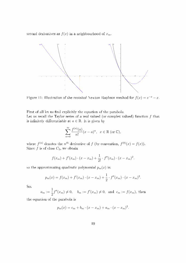
Figure 11: Illustration of the revisited Newton-Raphson method for f(x) = e−x−x.

First of all let us �nd explicitly the equation of the parabola.Let us recall the Taylor series of a real-valued (or complex-valued) function f thatis in�nitely di�erentiable at a ∈ R. It is given by

∞∑n=0

f (n)(a)

n!(x− a)n, x ∈ R (or C),

where f (n) denotes the nth derivative of f (by convention, f (0)(x) = f(x)).Since f is of class C2, we obtain

f(xm) + f ′(xm) · (x− xm) +1

2!· f ′′(xm) · (x− xm)2.

so the approximating quadratic polynomial pm(x) is:

pm(x) = f(xm) + f ′(xm) · (x− xm) +1

2· f ′′(xm) · (x− xm)2.

Set

am :=1

2f ′′(xm) 6= 0, bm := f ′(xm) 6= 0, and cm := f(xm), then

the equation of the parabola is

pm(x) = cm + bm · (x− xm) + am · (x− xm)2.

19

Now, we want to �nd the intersections of this parabola with the x-axis, which arethe solutions of pm(x) = 0. We see that pm(x) = 0 is a quadratic equation for thevariable (x− xm), so let us calculate the discriminant:

∆m = b2m − 4amcm.

Knowing this, we have two possible cases:

� ∆m < 0: In this case, pm(x) = 0 has no real solution for (x− xm). Since thereis no real solution for (x − xm), there is also no real solution for x satisfyingpm(x) = 0, so the parabola doesn't intersect the x-axis which implies that noiterative formula can be found. Thus, we can't use this method to �nd anapproximation of the root of f .

� ∆m ≥ 0: In this case, pm(x) = 0 has two real solutions for (x− xm) given by

(x− xm) =−bm+√b2m−4amcm2am

and (x− xm) =−bm−√b2m−4amcm2am

.Since we want xm+1 to be the intersection of the parabola with the x-axis, wewant that p(xm+1) = 0, thus

xm+1 − xm =−bm±√b2m−4amcm2am

= − bm2am±√b2m−4amcm

2am.

� If bm < 0: − bm2am

(1±

√b2m−4amcm

b2m

),

� If bm > 0: − bm2am

(1∓

√b2m−4amcm

b2m

).

Therefore, xm+1 is given by:

xm+1 = xm −bm

2am

(1±

√1− 4amcm

b2m

).

The problem now is that we found 2 values for xm+1, however we only want 1 valuebecause else, the algorithm would not work and would also be very complicatedsince the number of xm's would double after each iteration.

20

Figure 12: The problem is that the parabola (in blue) intersects the x-axis twice.

This means that we have to chose between the two solutions. Since we want toapproach the root of f , we choose the solution for xm+1 that is closer to the zero.We want this to be true for every xm, thus, the solution we choose for xm+1 mustalso be the one that is closer to xm. Looking at |xm+1−xm|, we see that the solutionwith the negative sign is closer to the root of f , therefore

xm+1 = xm −bm

2am

(1−

√1− 4amcm

b2m

), (6)

which is the iterative formula for the revisited Newton-Raphson method.

2.2.2 Geometric illustration

In order to get a better feeling on how the revisited Newton-Raphson methodcan be programmed, let us �rst illustrate it using GeoGebra. Under this link,https://www.geogebra.org/m/f4edtdfg, we created a GeoGebra program whichallows us to show graphically how this Newton-Raphson method works.

What happens in this program?The program requires, at the beginning, a real-valued function, a random initialvalue, two integers a, b for the interval [a, b], in which we want to �nd the zeroof the function; and the maximum number of iterations. Note that the maximumnumber of iterations is set to 6 since it is really time consuming writing out every

21

single iteration formula. The program stops when the maximum number of iterationsis achieved. Let us illustrate it with an example.

Example 2.6. Choose the real-valued function f(x) = x3 + 3, with initial guessx0 = −2 and [a, b] = [−10, 10] as the interval. After pressing the button Start, theprogram draws the arc of parabola p0 that is similar to the function at x0. Thisparabola has 2 points of intersection with the x-axis and the program denotes x1the one that is closer to x0. We obtain for the �rst iteration, x1 ≈ −1, 4. Then,the program is going to draw the arc of parabola p1 and denotes x2 its point ofintersection with the x-axis that is closer to x1 and after some iterations, we obtainthe correct approximation −1.44224957030741 with a tolerance of 15 digits.

22

Figure 13: Animation of the revisited Newton-Raphson method for f(x) = x3 + 3.

2.2.3 Algorithmic illustration

We are now ready to implement the revisited Newton-Raphson method in Python.The Python code is the following:

1 import sympy

2 import math

3 from sympy.parsing.sympy_parser import parse_expr

4 from sympy import *

5

6 x = symbols("x")

7 print("\nInput :\n")

8

9 f = input("Enter a function: ")

10 x0 = float(input("Enter an initial value: "))

11 t = float(input("Enter a desired tolerance of the root: "))

12 it = int(input("Enter the total number of iterations: "))

13

14 expr = parse_expr(f)

15 firstDeriv = expr.diff(x)

16 secondDeriv = firstDeriv.diff(x)

17

18 def Func(y):

19 return expr.subs(x,y)

20

21 def FirstDerivFunc(y):

22 return firstDeriv.subs(x,y)

23

24 def SecondDerivFunc(y):

25 return secondDeriv.subs(x,y)

26

27 def NewtonParabola(f, x0, t, it):

28 print("Let f(x) = ", f, ", then f'(x) = ", diff(f), ", and f''(

x) = ", diff(diff(f)), ".\n",sep = "")

23

29 x = x0

30 fx = Func(x)

31 dfx = FirstDerivFunc(x)

32 ddfx = SecondDerivFunc(x)

33

34 if t < 1e-15:

35 print("The desired tolerance is to high for Python. Choose

in between 1e-1 and 1e-15.")

36

37 elif 4*0.5*( ddfx)*(fx) > (dfx)**2 or 0.5* ddfx == 0 or dfx == 0:

38 print("The initial value does not have the required

condition. Hence , we can't use the 'revisited ' Newton -Raphson

method.")

39

40 else:

41 print("The initial value is given by x0 = ", x, ", and

applying the 'revisited ' Newton -Raphson method , we obtain\n",

sep = "")

42 for n in range(it):

43 y = x

44 x = x - dfx /(2*0.5* ddfx)*(1 - math.sqrt(1 - (4*0.5*(

ddfx)*(fx))/(dfx **2)))

45 fx = Func(x)

46 dfx = FirstDerivFunc(x)

47 ddfx = SecondDerivFunc(x)

48

49 if 4*0.5*( ddfx)*(fx) > (dfx)**2 or 0.5* ddfx == 0 or dfx

== 0:

50 print("We conclude that the sequence diverges.")

51 return None

52

53 elif abs(x - y) > t:

54 print("x_", n + 1, " = ", x, sep = "")

55

56 elif abs(x - y) <= t:

57 print("\nWe found a solution after ", n, "

iterations , given by ", y, ".\n", sep = "")

58 return None

59

60 print("We have surpassed the maximum number of iterations."

)

61

62

63 print("\nOutput :\n")

64

65 NewtonParabola(f, x0 , t, it)

Listing 2: Python code for the revisited Newton-Raphson method.

24

Explanation of the Python code.When running the Python code, the �rst step is to correctly plug in the function falong with an initial value, a desired tolerance of the correct root and the wantedmaximal number of iterations. From here on, the program transforms the pluggedin function, which is of type String, into an expression in order to de�ne the threefunctions Func(y), FirstDerivFunc(y), and SecondDerivFunc(y). These threefunctions just evaluate the plugged in function f at y, respectively the �rst andsecond derivative of the function at y.Then, the function NewtonParabola(f, x0, t, it), which takes the given functionf , the initial value x0, the tolerance t, and the maximum number of iterations it asthe only variables, �rst de�nes the iterative values by x, starting with x = x0, andfx to be the value of the function f evaluated at x, respectively dfx and ddfx tobe the �rst and second derivative of f evaluated at x. Now consider the followingthree cases.The �rst case is if the tolerance t is to high for Python, it prints out that one hasto choose a tolerance in between 1e− 1 and 1e− 15.The second case checks whether 4 · 1

2· ddfx · fx > (dfx)2, 1

2· ddfx = 0, or dfx = 0,

because if one of the three conditions is veri�ed, the iteration formula for the revisitedNewton-Raphson method fails. Hence, it prints out that the initial value does notful�ll the conditions for the iteration formula, and it is not applicable in this case.Lastly, if all the three conditions are not veri�ed, a for loop is introduced which goesover every n from 0 up to the maximum number of iterations minus one. Then inthis loop, it de�nes y to be equal to x, and replaces x using the iteration formula,which does not fail since all conditions were checked. It then proceeds to replace fxwith the value of the function evaluated at this new x, respectively dfx and ddfxwith the �rst and second derivative evaluated at x, and considers the following threecases.In the �rst case, it again has to check if one of the three conditions occurs. If it isthe case, it prints out that the sequence diverges, and returns None in order to endthe function at this point. Note that this return is essential, because otherwise itwould go back to the for loop.The second case is if the absolute value of the di�erence of x and y is greater thanthe tolerance t. If it is the case, it prints out the value of x, and de�nes this valueto be equal to the n+ 1th iteration. Note that since the for loop starts at 0, it hasto add 1 as x0 is already de�ned in the beginning. After this, it goes back to thefor loop.Lastly, if the absolute value of the di�erence is smaller or equal to the tolerance t,i.e. the desired root with the given tolerance is found, it prints out the number ofiterations needed for �nding this root, along with the value of this root. As before,in order to end the function at this point, it returns None.

25

If the for loop has gone over every n, i.e. it does not have found a solution, it printsout that the maximum number of iterations has been surpassed.

Example 2.7. Choose the same function as in Example 2.2, f(x) = x3 + 3, alongwith the same initial value x0 = −2 and the same tolerance of 1e − 10. Moreover,set the total number of iterations to 100. After running the Python code, we obtainthe following:

Figure 14: Input and output of Example 2.7.

Thus after 3 iterations, we obtain the correct root of the function f .

nbr. of iterations xm nbr. of correct digits0 -2,00000000000000 01 -1,40824829046386 22 -1,44225587295888 53 -1,44224957030741 15

Remark 2.3. We observe from the above table, that after each iteration, the numberof correct digits is roughly tripled. Intuitively, we can assume that the revisitedNewton-Raphson method has a cubic convergence.

Example 2.8. Choose the same function as above, f(x) = x3 + 3, along with thesame initial value x0 = −2, but this time we want a better tolerance, we want atolerance of 1e − 20. Moreover, set the total number of iterations to 100. Thetolerance we wish to have is to good for Python, thus after running the Pythoncode, we obtain the following:

26

Figure 15: Input and output of Example 2.8.

Example 2.9. Consider the function, f(x) = x4 + 3x2 + 2, along with an initialvalue x0 = 0, and a tolerance of 1e− 7. Moreover, set the total number of iterationsto 10. After calculating the derivative of f evaluated in x0 we �nd that f ′(x0) = 0,which implies that we can't use the iteration formula, since we divide by f ′(x0). Wesee that we cannot use Newton-Raphson's method, thus after running the Pythoncode, we obtain the following:

Figure 16: Input and output of Example 2.9.

Example 2.10. Let f(x) = x4 + 3x2 + 2 be a function, and choose an initial valuex0 = 4, and a tolerance of 1e−10. Moreover, set the total number of iterations to 20.After calculating f(x0), f

′(x0) and f′′(x0), we see that 4 · 1

2·f ′′(x0) ·f(x0) > f ′(x0)

2,so that we cannot use the iteration formula since the value in the square root isnegative. In this case, the Python code returns the following:

27

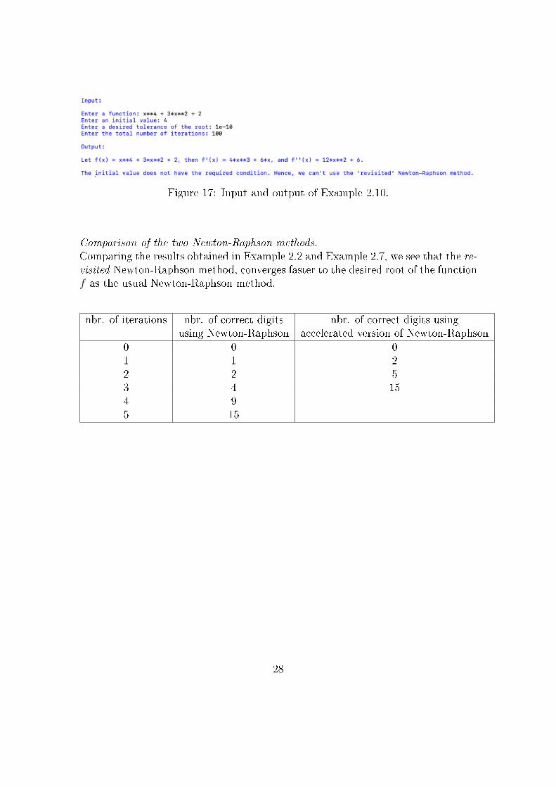
Figure 17: Input and output of Example 2.10.

Comparison of the two Newton-Raphson methods.Comparing the results obtained in Example 2.2 and Example 2.7, we see that the re-visited Newton-Raphson method, converges faster to the desired root of the functionf as the usual Newton-Raphson method.

nbr. of iterations nbr. of correct digits nbr. of correct digits usingusing Newton-Raphson accelerated version of Newton-Raphson

0 0 01 1 22 2 53 4 154 95 15

28

3 Factorising polynomials over �nite �elds using Berlekamp's

algorithm

In the section above, we explained the Newton-Raphson method, one of many meth-ods that helps solving polynomial equations over real numbers. Now, it might beinteresting to look at a method to solve polynomial equations over �nite �elds. Thealgorithm we are going to explain is the so called Berlekamp algorithm.Berlekamp's algorithm is named after the mathematician Elwyn Berlekamp, whodeveloped it in 1967, and it is an algorithm used to factorise polynomials withcoe�cients over �nite �elds. For years, Berlekamp's algorithm was the dominantmethod for solving polynomial equations over �nite �elds, until 1981, when theCantor-Zassenhaus algorithm was created.Berlekamp's algorithm consists mainly of matrix reduction and polynomial greatestcommon divisor (short gcd) computations. The input is a polynomial P of degreen ∈ N with coe�cients in a given �nite �eld and the output is a polynomial b withcoe�cients in the same �nite �eld, that divides P . Applying the algorithm recur-sively to these subsequent divisors b, we �nd the decomposition of P into irreduciblepolynomials.

3.1 General statement

Let

� Fp[x] be a �nite �eld of size p ∈ P (where P is the set of all prime numbers),e.g. F3[x] is the set of polynomials with coe�cients in F3 = {0, 1, 2} (we canimagine it as F3 ≡ N mod 3),

� P (x) ∈ Fp[x] be a polynomial of degree n ∈ N with Fp-coe�cients in x.

The goal is to factorise P (x) in Fp[x], i.e. to �nd irreducible factors p1(x), ..., pk(x)∈Fp[x], where k ∈ N is unknown, such that

P (x) = p1(x) · ... · pk(x) =k∏i=1

pi(x).

Note that if k = 1, then P (x) = p(x) and we conclude that P (x) is already irre-ducible.In addition, we assume that P (x) is square-free, i.e. that all the pi's are distinct.One of the reasons why we assume that P (x) is square-free is that by taking the gcdof P (x) and the derivative of P (x) with respect to x, denoted by P ′(x) = d

dxP (x)

we always have that gcd(P (x), P ′(x)) = 1. Note that this is the case because every

29

multiple factor of a polynomial P over a �eld introduces a nontrivial common factorof P and P ′. If P (x) was not square-free, then we would have found a divisor ofP (x) by calculating gcd(P (x), P ′(x)).The important question now is, how to �nd the irreducible factors pi(x) of P (x)∀i ∈ {1, ..., k}. In order to do this, consider a polynomial

G(x) :=∏a∈Fp

(b(x)− a) ∈ Fp[x],

that is divisible by P (x) and that is easier to factorise, where b(x) ∈ Fp[x]. Thispolynomial is divisible by P (x) if

P (x) =k∏i=1

pi(x) =∏a∈Fp

gcd(P (x), b(x)− a). (7)

Also, since Fp is a �nite �eld, we can replace in the identity xp− x =∏

a∈Fp(x− a),

x by our b(x) and we obtain:

b(x)p − b(x) =∏a∈Fp

(b(x)− a) = G(x).

One may ask how the polynomials b(x) are found.In fact, we want that P (x) divides G(x) and we know that G(x) = b(x)p − b(x),thus we need to �nd b(x) such that

b(x)p ≡ b(x) mod P (x).

Note that these polynomials b(x) form a subalgebra of the factor ring

R =Fp[x]

〈P (x)〉

called Berlekamp subalgebra. Since P (x) divides the polynomial G(x), we concludeby (7) that if the gcd(P (x), b(x) − a)'s are irreducible, the pi

′s must be given bypi(x) = gcd(P (x), b(x) − a) for a ∈ Fp, and b(x) in the Berlekamp subalgebra. Ifsome gcd(P (x), b(x) − a) are not irreducible, we use the algorithm on these poly-nomials, until every polynomial is irreducible.To �nd the pi's, we have to �nd all the polynomials b(x) from the Berlekamp sub-algebra, i.e. all polynomials b(x) satisfying b(x)p ≡ b(x) mod P (x). In order to dothis, we use the following observation.

30

Consider a n × n matrix M = (mi,j)0≤i,j≤n−1, where the coe�cients mi, j are givenby the following congruence:

xip ≡n−1∑j=0

mi,jxj mod P (x). (8)

We can now show that each eigenvector b =

b0...

bn−1

ofM with eigenvalue 1 provides

a polynomial b(x) given by

b(x) :=n−1∑l=0

blxl, (9)

that satis�es b(x)p ≡ b(x) mod P (x). Indeed,

b(x)p(9)=

(n−1∑l=0

blxl

)p

Fp=

n−1∑l=0

bpl xlp Fp

=n−1∑l=0

blxlp

(8)≡

n−1∑l=0

bl

n−1∑j=0

ml,jxj mod P (x)

linearity=

n−1∑j=0

(n−1∑l=0

ml,jbl

)xj mod P (x)

eigenvectors=

∑j

bjxj mod P (x)

= b(x) mod P (x).

Finding all the eigenvectors of M for the eigenvalue 1 is equivalent to �nding thenull space (i.e. the Kernel) of the matrix (M − 1 · In), where In is the n×n identitymatrix. Thus to �nd the polynomials b(x) of the Berlekamp subalgebra, it su�cesto �nd the basis vectors of the null space of (M − In).Finally, we obtain the factors pi(x)∀i ∈ {1, ..., k} by calculating for each a ∈ Fpand for every vector b(j) in the null space of (M − In):

gcd(P (x), b(j)(x)− a) ∀j,

where b(j)(x) is the polynomial corresponding to the vector b(j) and with the conditionsthat

� b(j) = (1, 0, ..., 0) can be rejected and

31

� we continue until we have determined k := n− r = deg(P (x))− rang(M − In)factors of P (x) (i.e. until we have found k di�erent gcd(P (x), b(j)(x)−a) 6= 1).

Hence, we can summarize Berlekamp's algorithm in the following 4 steps.

Step 1: Verify that the polynomial is square-free, i.e check if gcd(P (x), P ′(x)) = 1.

Step 2: Calculate the matrix M = (mi,j)n×n, by computing

xip ≡n−1∑j=0

mi,jxj mod P (x). ∀i = 0, ..., n− 1.

Step 3: Find the basis of the null space of (M − In).

Step 4: Calculate for each b(j) 6= (1, 0, ..., 0) in the basis of the null space of (M−In)and for every a ∈ Fp:gcd(P (x), b(j)−a) until n− r = deg(P (x))− rang(M − In) factors of P (x)have been found.

Remark 3.1. In the case where the leading coe�cient of the polynomial we wishto factorise is not 1, we need to multiply the obtained factorisation by the leadingcoe�cient. For an application, look at Example 3.5.

3.2 Algorithmic illustration

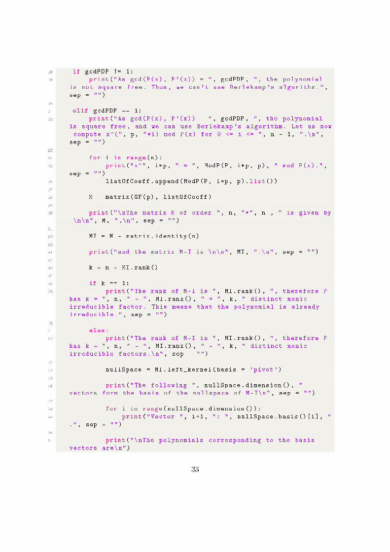
We are now ready to implement Berlekamp's algorithm in Sage. The Sage code isthe following:

1 def ModP(P, a, p):

2 R.<x> = PolynomialRing(GF(p), 'x')

3 S.<x> = R.quotient(P)

4

5 return x^a

6

7

8 def Berlekamp(P, p):

9 R.<x> = PolynomialRing(GF(p), 'x')

10 P = R(P.list())

11 n = P.degree ()

12 c = P.lc()

13 dP = derivative(P)

14 listOfCoeff = []

15 print("Let P(x) = ", P, ". Then , P'(x) = ", dP , ".\n", sep = ""

)

16

17 gcdPDP = P.gcd(dP)

32

18 if gcdPDP != 1:

19 print("As gcd(P(x), P '(x)) = ", gcdPDP , ", the polynomial

is not square free. Thus , we can't use Berlekamp 's algorithm.",

sep = "")

20

21 elif gcdPDP == 1:

22 print("As gcd(P(x), P '(x)) = ", gcdPDP , ", the polynomial

is square free , and we can use Berlekamp 's algorithm. Let us now

compute x^(", p, "*i) mod P(x) for 0 <= i <= ", n - 1, ".\n",

sep = "")

23

24 for i in range(n):

25 print("x^", i*p, " = ", ModP(P, i*p, p), " mod P(x).",

sep = "")

26 listOfCoeff.append(ModP(P, i*p, p).list())

27

28 M = matrix(GF(p), listOfCoeff)

29

30 print("\nThe matrix M of order ", n, "*", n , " is given by

\n\n", M, ",\n", sep = "")

31

32 MI = M - matrix.identity(n)

33

34 print("and the matrix M-I is \n\n", MI, ".\n", sep = "")

35

36 k = n - MI.rank()

37

38 if k == 1:

39 print("The rank of M-I is ", MI.rank(), ", therefore P

has k = ", n, " - ", MI.rank(), " = ", k, " distinct monic

irreducible factor. This means that the polynomial is already

irreducible.", sep = "")

40

41 else:

42 print("The rank of M-I is ", MI.rank(), ", therefore P

has k = ", n, " - ", MI.rank(), " = ", k, " distinct monic

irreducible factors .\n", sep = "")

43

44 nullSpace = MI.left_kernel(basis = 'pivot')

45

46 print("The following ", nullSpace.dimension (), "

vectors form the basis of the nullspace of M-I\n", sep = "")

47

48 for i in range(nullSpace.dimension ()):

49 print("Vector ", i+1, ": ", nullSpace.basis ()[i], "

.", sep = "")

50

51 print("\nThe polynomials corresponding to the basis

vectors are\n")

33

52

53 for i in range(nullSpace.dimension ()):

54 print("b", i+1, "(x) = ", R(list(nullSpace.basis()[

i])), ".", sep = "")

55

56 print("\nThen , successively calculate\n")

57

58 for i in range(1, nullSpace.dimension ()):

59 listOfMonicPolys = []

60

61 for j in range(p):

62 print("gcd(P(x), b", i+1, "(x) - ", j, ") = ",

P.gcd(R(list(nullSpace.basis()[i])) - j), ".", sep = "")

63

64 if P.gcd(R(list(nullSpace.basis ()[i])) - j) !=

1:

65 listOfMonicPolys.append(P.gcd(R(list(

nullSpace.basis ()[i])) - j))

66

67 if len(listOfMonicPolys) != k:

68 print("\nSince P has ", k, " distinct monic

irreducible factors , but from the above one obtains\n", sep = ""

)

69

70 print("P(x) = (", ")(".join(str(e) for e in

listOfMonicPolys), ").\n", sep = "")

71

72 if i + 2 > nullSpace.dimension ():

73 for t in range(p):

74 for e in listOfMonicPolys:

75 if e.degree () > 1 and e(x = t) ==

0:

76 listOfMonicPolys.remove(e)

77 print("Since ", e, " is not

irreducible in F", p, "[x], we use Berlekamp 's algorithm to

factorise this polynomial .\n", sep = "")

78

79 listOfMonicPolys = Berlekamp2(e

, p) + listOfMonicPolys

80 print("We find that , ", e, " =

(", ")(".join(str(e1) for e1 in Berlekamp2(e, p)), ").\n", sep =

"")

81

82 if len(listOfMonicPolys) == k:

83 print("Thus , the final

factorisation of P is\n")

84 if c == 1:

85 print("P(x) = (", ")(".

join(str(e1) for e1 in listOfMonicPolys), ").", sep = "")

34

86 break

87 else:

88 print("P(x) = ", c, "("

, ")(".join(str(e1) for e1 in listOfMonicPolys), ").", sep = "")

89 break

90 else:

91 print("Thus , repeat the procedure for b", i

+2, "(x).\n",sep = "")

92 continue

93

94 else:

95 print("\nSince P has ", k, " distinct monic

irreducible factors , our desired factorisation of P is\n", sep =

"")

96 if c == 1:

97 print("P(x) = (", ")(".join(str(e) for e in

listOfMonicPolys), ").", sep = "")

98 break

99 else:

100 print("P(x) = ", c, "(", ")(".join(str(e)

for e in listOfMonicPolys), ").", sep = "")

101 break

Listing 3: Sage code for Berlekamp's algorithm.

Explanation of the Sage code.The function ModP(P , a, p), which takes a polynomial P , a positive integer a,and a prime number p as the only 3 variables, �rst creates a polynomial ring overa �nite �eld of size p, and denotes it by R. In fact, R = GF (p)[x] = Fp[x]. It thenuses this polynomial ring R to create the quotient ring R/〈P 〉, which was also calledthe Berlekamp subalgebra. Lastly, this function returns the result of xa mod P inR. More speci�cally, this function will be helpful to compute xip mod P .

The main function Berlekamp(P , p), which takes a polynomial P , and a primenumber p as the only 2 variables, again creates a polynomial ring over a �nite �eldof size p, and denotes it by R. It then has to rede�ne the polynomial P in thispolynomial ring, so that P ∈ R. Note that P.list() returns a list of the coe�cientsof P , and R(P.list()) generates the corresponding polynomial to those coe�cientsin R. It then de�nes n to be the degree of P , c to be the leading term of P , dP tobe the derivative of P , listOfCoeff to be an empty list, which will be helpful toconstruct the matrix M , and gcdPDP to be the gcd of P and dP .Now, if gcdPDP is not equal to 1, it prints out gcdPDP along with a messagesaying that Berlekamp's algorithm is not applicable.On the other hand, if gcdPDP is equal to 1, P is square-free, and it computes xip

mod P for i starting from 0 up to n − 1, using the de�ned function ModP(P , ip,p). Simultaneously, it adds a list of the coe�cients of each xip mod P to listOfCoe�.

35

Thus, it de�nes M to be the matrix over the �nite �eld of size p, the matrix MI tobe the di�erence of M and the n× n identity matrix, and k to be the di�erence ofn and the rank of MI. Now, consider two cases.If k is equal to one, it prints out that P is already irreducible.On the other hand, if k is not one, it prints out that P has k distinct monic irre-ducible factors. It then de�nes nullSpace to be the null space of MI, and extractsits basis vectors by using nullSpace.basis[i], where i ranges from 0 up to the di-mension of nullSpace minus one. This function just returns the i-th basis vectorof nullSpace. The corresponding polynomials to those basis vectors are given byR(list(nullSpace.basis()[i])), where again i ranges from 0 up to the dimension ofnullSpace minus one, and they are denoted by bi+1(x). Note that each basis vectorhas to be transformed into a list by using the function list() in order to obtain thecorresponding polynomial to those coe�cients.Now, the �rst for loop ranges from 1 up to the dimension of nullSpace minus one,and then de�nes listOfMonicPolys to be an empty list, which will be helpful tomemorize all monic irreducible factors. Then, the second for loop ranges from 0 upto p− 1, and in this loop, it computes the gcd of P and bi+1(x)− j. Note that sincei starts at 1, b1(x) will not be considered as it is always rejected. Furthermore, ifthe gcd of P and bi+1(x)− j is not equal to 1, it will be added to listOfMonicPolys.Again, consider the following two cases.If the length of listOfMonicPolys is not equal to k, it prints out the obtained fac-torisation using listOfMonicPolys, which is not the wanted one, since there aren't kmonic irreducible factors. Now it has to consider two cases.If there aren't no more bi+1(x)s to check, a �rst for loop which goes through every tfrom 0 up to p− 1, and a second for loop which goes over every element e in listOf-MonicPolys are introduced, in order to check which element e is not irreducible.Hence, it must check if the degree of e is greater than 1, and if there is a t forwhich e is zero when evaluating at t. If the two conditions are veri�ed, the elemente is removed from listOfMonicPolys, since only irreducible factors are memorized inthis list. Then, it replaces listOfMonicPolys by the sum of Berlekamp2(e, p) andlistOfMonicPolys. Note that this is a modi�ed function of the current function, andjust returns a list of all monic irreducible factors of e. Now if all k monic irreduciblefactors are found, it prints out the obtained factorisation using listOfMonicPolys,and by using break, it jumps out of both for loops, and reaches the end of the de�nedfunction. Note that it distinguishes between the cases whether c is equal to 1 or notfor a better visualization.If there are any bi+1(x)s left to check, it has to jump back to the �rst loop by usingcontinue.On the other side, if the length of listOfMonicPolys is indeed equal to k, it printsout the obtained factorisation using listOfMonicPolys, and by using break, it jumps

36

out of the �rst for loop, and reaches the end of the de�ned function. Again, it dis-tinguishes between the cases whether c is equal to 1 or not for a better visualization.

Example 3.1. If we consider the polynomial P (x) = x2 + 2x + 1 over the �nite�eld F3, then we cannot use Berlekamp's algorithm since it is not square free. Inthis case, the Sage program returns the following:

Figure 18: Output of Example 3.1.

Example 3.2. Consider the polynomial P (x) = x8 + 3x5 + 2x + 1 over the �nite�eld F5. After calculating the rank of the matrixM−I8 we �nd that the polynomialis already irreducible. In this case, the Sage program returns the following:

Figure 19: Output of Example 3.2.

Example 3.3. Consider the polynomial P (x) = x3 + x2 + x+ 1 over the �nite �eldF5. Let us factorise it using Berlekamp's algorithm. After running the Sage code,we obtain the following:

37

Figure 20: Output of Example 3.3.

Example 3.4. Let P (x) = x5 + x3 + x2 + 1 be a polynomial over the �nite �eld F5.We will factorise it using Berlekamp's algorithm, however after having considered allthe gcd(P (x), b(j)(x)− a), where the b(j)(x)'s are the polynomials corresponding tothe basis vectors and a ∈ F7, we still haven't found the correct number of irreduciblefactors. That is why we have to factorise the polynomials, which we obtained, thatare not irreducible. The Sage algorithm returns the following:

38

Figure 21: Output of Example 3.4.

Example 3.5. Consider the polynomial P (x) = 2x4+5x3+3x+1 over the �nite �eldF7. We will factorise it using Berlekamp's algorithm, however we have to multiplythe �nal factorisation by the leading coe�cient since it is not equal to 1 but 2. Afterrunning the Sage code, we obtain the following:

39

Figure 22: Output of Example 3.5.

4 Solving polynomial congruence equations using

Hensel's Lemma

After having studied a method to factorise polynomials over �nite �elds, it's inter-esting to look at a method that solves polynomial equations modulo pn, where p isa prime number and n is a natural number greater than 1. The so called HenselLemma allows us to �nd such solutions.Also known as Hensel's lifting Lemma and named after Kurt Hensel, this is a resultthat uses Berlekamp's algorithm and a variant of Newton's approximation to solveequations modulo pn. In fact, we start from a solution modulo p, that we obtainusing Berlekamp's algorithm and "improve" it to solutions modulo powers of p byusing a variant of Newton's approximation.

4.1 General statement

Let

� P (x) be a polynomial with integer coe�cients,

� p be a prime number,

40

� n be a positive integer greater than 1,

� a be a solution of P (x) ≡ 0 mod pn such that P ′(a) 6≡ 0 mod p and

� b be a solution of P (x) ≡ 0 mod pn+1 such that b ≡ a mod pn.

Since b ≡ a mod pn, there exists an integer t such that

b = a+ tpn.

The goal now is to determine t. First, we use the Taylor series expansion on Paround a:

P (x) = P (a) +P ′(a)

1!(x− a) +

P ′′(a)

2!(x− a)2 +

P ′′′(a)

3!(x− a)3 + ....

For x = a+ tpn we obtain the following:

P (a+ tpn) = P (a) + P ′(a)tpn +P ′′(a)

2(tpn)2 +

P ′′′(a)

6(tpn)3 + ....

So that, the above equation mod pn+1 is:

P (a+ tpn) ≡ P (a) + P ′(a)tpn +P ′′(a)

2(tpn)2 +

P ′′′(a)

6(tpn)3 + ... mod pn+1.

For m ≥ 2, we have that (tpn)m ≡ 0 mod pn+1. This implies that:

P (a+ tpn) ≡ P (a) + P ′(a)tpn mod pn+1.

We also know that P (b) ≡ 0 mod pn+1 and b = a+ tpn, thus:

P (a) + P ′(a)tpn ≡ 0 mod pn+1.

This implies that:P ′(a)tpn ≡ −P (a) mod pn+1.

Since pn divides P ′(a)tpn and −P (a) (because P (a) ≡ 0 mod pn), we have that:

P ′(a)t ≡ −P (a)

pnmod p.

Also, P ′(a) 6≡ 0 mod p which means that p doesn't divide P ′(a), and p is prime,thus gcd(P ′(a), p) = 1 which implies that P ′(a) and p are coprime. We concludethat P ′(a)−1 exists and thus we obtain:

t ≡ − P (a)

P ′(a)pnmod p.

In addition, this t is unique.From this, we can derive Hensel's Lemma that states the following:

41

Lemma 4.1. Let p be a prime number and let P (x) be a polynomial with integer(or p-adic integer) coe�cients. Let also, n and an be integers such that an is asolution of P (x) ≡ 0 mod pn satisfying P ′(an) 6≡ 0 mod p.Then, for m being an integer, there exists an integer an+m such that

P (an+m) ≡ 0 mod pn+m

andan+m ≡ an mod pn.

Furthermore, this an+m is unique modulo pk+m and can be computed explicitly by

an+m ≡ an −P (an)

P ′(an)mod pn+m.

This means that, if a1 satis�es P (a1) ≡ 0 mod p and P ′(a1) 6≡ 0 mod p, thenwe can obtain a solution an+1 of P (x) ≡ 0 mod pn+1 by the recursive formula

an+1 ≡ an − P (an)P ′(an)

mod pn+1.

A proof of this Lemma can be found in [12].

4.2 Algorithmic illustration

We are now ready to implement Hensel's Lemma in Sage. The Sage code is thefollowing:

1 def Hensel(P, p, n):

2 R.<x> = PolynomialRing(GF(p), 'x')

3 RP = P

4 P = R(P.list())

5 dP = derivative(P)

6

7 if Berlekamp(P, p) == 0:

8 print("The polynomial is not square free , thus we can't use

Hensel 's Lemma.")

9

10 elif Berlekamp(P, p) == 1:

11 print("The polynomial is already irreducible , thus we can't

use Hensel 's Lemma.")

12

13 elif Berlekamp(P, p) == []:

14 print("The polynomial has no solution in F", p, "[x], thus

we can't use Hensel 's Lemma.", sep = "")

15

16 else:

17 print("Let P(x) = ", RP , ".\n", sep = "")

18

42

19 print("We want to obtain all solutions of P(x) = 0 mod ", p

, "^", n, " using Hensel 's Lemma.\n", sep = "")

20

21 print("In order to apply Hensel 's Lemma , we first find all

solutions to P(x) = 0 mod ", p, ".\n", sep = "")

22

23 roots = Berlekamp(P, p)

24 print("By Berlekamp 's algorithm , we get that ", ", ".join(

str(r) for r in roots), " is a solution of P(x) = 0 mod ", p, "

.\n", sep = "")

25

26 print("Let a1 = ", ", ".join(str(r) for r in roots),". Then

, we need to verify that P'(a1) mod ", p, " is not equal to 0.\n

", sep = "")

27

28 print("The derivative of P is given by P'(x) = ", dP , ".

Thus ,\n", sep = "")

29

30 for r in roots:

31 print("P '(", r, ") = ", dP(x = r), " mod ", p, ".", sep

= "")

32

33 if dP(x = r) == 0:

34 roots.remove(r)

35

36 if len(roots) == 0:

37 print("We cannot apply Hensel 's Lemma , since all the

above derivatives are equal to 0.")

38

39 elif len(roots) == 1:

40 print("\nSo , Hensel 's Lemma can be applied to ", " and

".join(str(r) for r in roots), ".\n",sep = "")

41

42 a1 = roots [0]

43 dPx = 1/dP(x = a1)

44 print("First set a1 = ", a1 , ". Then , we calculate [P'(

", a1 , ")]^(-1) = [", dP(x = a1),"]^(-1) = ", dPx , " mod ", p, "

.\n", sep = "")

45

46 a = [a1]

47 print("Thus by Hensel 's Lemma , we obtain\n")

48

49 k = 1

50 for j in range(2, n + 1):

51 R.<x> = PolynomialRing(Zmod(p^j), 'x')

52 P = R(RP.list())

53 print("a", j, " = a", k, " - P(a", k, ")*[P'(a", k,

")]^(-1) mod ", p, "^", j, sep = "")

43

54 print("a", j, " = ", a[0], " - P(", a[0], ")*[P'(",

a[0], ")]^(-1) mod ", p, "^", j, sep = "")

55 print("a", j, " = ", a[0], " - ", P(x = Integer(a

[0])), "*", dPx , " mod ", p, "^", j, sep = "")

56 print("a", j, " = ", ( Integer(a[0]) - P(x =

Integer(a[0])) * Integer(dPx) ) % p^j, " mod ", p, "^", j, "\n",

sep = "")

57 a[0] = ( Integer(a[0]) - P(x = Integer(a[0])) *

Integer(dPx) ) % p^j

58 k += 1

59

60 print("So x = ", a[0], " is a solution to P(x) = 0 mod

", p, "^", n, ".", sep = "")

61

62 elif len(roots) != 1:

63 print("\nSo , Hensel 's Lemma can be applied to ", ", ".

join(str(r) for r in roots), ".\n",sep = "")

64

65 a1 = roots [0]

66 dPx = 1/dP(x = a1)

67 print("First set a1 = ", a1 , ". Then , we calculate [P'(

", a1 , ")]^(-1) = [", dP(x = a1),"]^(-1) = ", dPx , " mod ", p, "

.\n", sep = "")

68

69 i = 0

70 while i < len(roots):

71 a = [roots[i]]

72 print("Thus by Hensel 's Lemma , we obtain\n")

73

74 k = 1

75 for j in range(2, n + 1):

76 R.<x> = PolynomialRing(Zmod(p^j), 'x')

77 P = R(RP.list())

78 print("a", j, " = a", k, " - P(a", k, ")*[P'(a"

, k, ")]^( -1) mod ", p, "^", j, sep = "")

79 print("a", j, " = ", a[0], " - P(", a[0], ")*[P

'(", a[0], ")]^( -1) mod ", p, "^", j, sep = "")

80 print("a", j, " = ", a[0], " - ", P(x = Integer

(a[0])), "*", dPx , " mod ", p, "^", j, sep = "")

81 print("a", j, " = ", ( Integer(a[0]) - P(x =

Integer(a[0])) * Integer(dPx) ) % p^j, " mod ", p, "^", j, "\n",

sep = "")

82 a[0] = ( Integer(a[0]) - P(x = Integer(a[0])) *

Integer(dPx) ) % p^j

83 dPx = 1/dP(x = a[0])

84 k += 1

85

86 print("So x = ", a[0], " is a solution to P(x) = 0

mod ", p, "^", n, ".", sep = "")

44

87

88 i += 1

89 if i == len(roots):

90 break

91 else:

92 a1 = roots[i]

93 dPx = 1/dP(x = a1)

94 print("\nSetting a1 = ", a1, ". Then , we

calculate [P '(", a1, ")]^( -1) = [", dP(x = a1),"]^(-1) = ", dPx ,

" mod ", p, ".\n", sep = "")

Listing 4: Sage code for Hensel's Lemma.

Explanation of the Sage code.

Remark 4.1. For the explanation of the function Berlekamp(P , p), we referSubsection 3.2 with the following modi�cations. Note that those modi�cations arenecessary in order to use its result in the main function. The only di�erence is thatall the print()'s are removed, and where the function is out of arguments, a returnis added which returns a value that will be used in the main function.For instance, if gcdPDP is not equal to one, it returns 0, i.e. that is the case wherethe polynomial is not square free.If k is equal to one, it returns 1, i.e. the case where the polynomial is alreadyirreducible.Lastly, if the length of listOfMonicPolys is equal to k, i.e. if all k monic irreduciblefactors are found, it �rst de�nes an empty list listOfRoots, which will be helpful tosave all roots of the k monic factors. Then, the for loop goes over all the elementsof listOfMonicPolys, and checks if the element e has a root in Fp[x]. Note thate.roots() returns a list of a pair (a, b), where a is the root of e in Fp[x], and b isthe multiplicity of a. Also, if e has no roots in Fp[x], it returns an empty list, thatis why it checks if e.roots() is nonempty. Then, in this case, it adds the root a tolistOfRoots. Note that e.roots()[0] returns the pair (a, b), and e.roots()[0][0] returnsthe root a. At the end, it returns listOfRoots, which contains all the roots of P .

Let us now move on to the explanation of the function Hensel(P , p, n) whichtakes P , p and n as the only 3 variables, where P is a polynomial, p is a primenumber, and n is a natural number greater or equal than 2. Then as always, itcreates a polynomial ring over a �nite �eld of size p, it rede�nes the polynomial Pin this polynomial ring, and de�nes dP to be the derivative of P . Now, consider thefollowing four cases.The �rst case, is if the function Berlekamp(P , p) returns 0, then it prints out thatthe polynomial is not square free, and Hensel's Lemma is not applicable.The second case, if Berlekamp(P , p) returns 1, it prints out that the polynomialis already irreducible, and again Hensel's Lemma is not applicable.

45

In the third case, where Berlekamp(P , p) returns an empty list, it prints out thatthe polynomial has no solutions in the polynomial ring, and again Hensel's Lemmais not applicable. Note that from Remark 4.1, listOfRoots can be empty if all kfactors do not have a root in Fp[x].Lastly, if none of the �rst three cases are true, it de�nes roots to be the list containingall the roots of P (x) ≡ 0 mod p. Then, in order to verify that the derivativeevaluated at each root is not equal to zero, it uses a for loop which goes over all theelements in roots. It �rst prints out the derivative at the element, and then checksif the derivative at the element is equal to zero, and if it is the case, it removesthis element out of roots, since Hensel's Lemma only considers those, where thederivative is di�erent from zero. Again, consider the following three cases.If the length of roots is equal to zero, i.e. if all element are removed from the listroots, it prints out that Hensel's Lemma is not applicable, as all the derivatives areequal to 0.On the other hand, if the length of roots is equal to one, i.e. there is only one rootthat satis�es Hensel's Lemma, it �rst de�nes a1 to be equal to this root by usingroots[0], dPx to be the inverse of the derivative evaluated at a1, and a to be a listcontaining a1. Then, by de�ning k to be equal to 1, in the for loop, where j rangesfrom 2 up to n, it creates a new polynomial ring over the �eld Z/pnZ. Then, ithas to rede�ne the polynomial P over this new polynomial ring in order to ensurethat all calculations are considered in this polynomial ring. It then prints out thecalculations for aj mod pj, and replaces the �rst element in a by this new calculatedvalue, and k is augmented by one. Note that in order to do these calculations in thispolynomial ring, it has to transform every single value into an integer by using thefunction Integer(). Then, if j is still in the range, it repeats those calculations. If itis out of range, it prints out the obtained result, which is the solution to P (x) ≡ 0mod pn.Lastly, if the length of roots is not equal to one, i.e. there is more than one rootsatisfying Hensel's Lemma, it again de�nes a1 to be the �rst root in roots, and dPxto be the inverse of the derivative evaluated at a1. By de�ning i to be equal to zero,a while loop is being introduced, which will be executed if i is less than the length ofroots. Then, in this while loop, it de�nes a to be the i-th element of roots, and doesagain the same as explained above. After this, i is augmented be one, and checks ifi is equal to the length of roots. If it is the case, it uses break to jump out of thewhile loop, and it reaches the end of the function. Note that this condition tells uswhether there are any elements left in roots or not. If i is not equal to the lengthof roots, it de�nes a1 to be the i-th element of roots, dPx to be the inverse of thederivative evaluated at a1, goes back to the while loop, and repeats the procedure,until i is equal to len(roots).

46

Example 4.1. Consider the polynomial P (x) = x2+2x+1 and let us solve P (x) ≡ 0mod 37, then we cannot use Berlekamp's algorithm since it is not square free andconsequently, we cannot use Hensel's algorithm. In this case, the Sage programreturns the following:

Figure 23: Output of Example 4.1.

Example 4.2. Consider the polynomial P (x) = x8 + 3x5 + 2x + 1. We wish to�nd the solutions of P (x) ≡ 0 mod 55, but we �nd that the polynomial is alreadyirreducible and thus, the equations has no solution. In this case, the Sage programreturns the following:

Figure 24: Output of Example 4.2.

Example 4.3. Consider the equation P (x) ≡ 0 mod 73, where P (x) = 2x4 +5x3 +3x + 1. We will solve it using Hensel's Lemma, however there are no solutionsof P (x) ≡ 0 mod 7, so that the equation we wish to solve also has no solution,according to Hensel's Lemma. After running the Sage code, we obtain the following:

Figure 25: Output of Example 4.3.

47

Example 4.4. Consider the polynomial equation modulo 113 given by: P (x) ≡ 0mod 113, where P (x) = x12 + 2x8 + x7 + 3x2 + 1. Let us solve it using Hensel'sLemma. After running the Sage code, we obtain the following:

Figure 26: Output of Example 4.4.

Example 4.5. Let P (x) = x3 + x2 + x + 1 be a polynomial and let us solve theequation P (x) ≡ 0 mod 56 us ing Hensel's Lemma. The Sage algorithm returns thefollowing:

48

Figure 27: Output of Example 4.5.

5 Conclusion

The main purpose of this research project, which is the study of methods used forsolving polynomial equations over real numbers and over �nite �elds, has given usthe opportunity to analyse and explore several results in greater detail.In our journey through polynomial equations, we did not only learn new methods andalgorithms, such as Newton-Raphson's method, Berlekamp's algorithm and Hensel'sLemma, but we also had the chance to illustrate them practically. This allowed us toverify the learned properties in our animations and implement them in our programs.Moreover, the realisation of these methods and algorithms in Python and Sage havegiven us the opportunity to better understand the theory studied beforehand. Since,we had to program codes that give the factorisation of given polynomials in given

49

�elds, we had to write down step by step how it's done. By decomposing the theoryand programming each execution step, we had to make sure we fully understood theconcept behind it.Thus, programming not only helped us understand the algorithms, but was also amore practical way to understand the theory, and how it can be applied to solvepolynomial equations.To conclude, we can say that the option "Experimental Mathematics" not onlyallows students to study mathematical methods and algorithms, but also discover theresearch of mathematics and explore subjects in greater detail, as using programminglanguages Python and Sage to implement the theory learned.

Acknowledgement. The three authors would like to thank Prof. Dr. Gabor Wieseand Guendalina Palmirotta for having supervised this project in the ExperimentalMathematics Lab of University of Luxembourg.

50

References

[1] Quadratic equation. Wikipedia, December 2020. Page Version ID: 43588.

[2] Cubic equation. Wikipedia, December 2020. Page Version ID: 180787.

[3] Méthode de Cardan. Wikipedia, October 2020. Page Version ID: 153526.

[4] Algebra Identities: Standard Identities Of Algebra, De�nition & Examples.https://www.embibe.com/exams/algebra-identities/

[5] Jean-Luc Marichal, Analyse numérique, Université du Luxembourg, Version2013-2014.

[6] Guendalina Palmirotta, On the Geometry of Householder's and Halley's Meth-ods, Student project, University of Luxembourg, Winter semester 2015-2016.

[7] Newton's method. Wikipedia, December 2020. Page Version ID: 22145.

[8] Sajid Hanif, Muhammad Imran, Factorization Algorithms for Polynomialsover Finite Fields, Linnaeus University, School of Computer Science, Physicsand Mathematics, 2011-05-03.https://www.diva-portal.org/smash/get/diva2:414578/FULLTEXT01.

pdf

[9] Berlekamp-Algorithmus. Wikipedia, June 2018. Page Version ID: 1875740.

[10] Berlekamp's algorithm. Wikipedia, December 2020. Page Version ID: 6057100.

[11] Hensel's lemma. Wikipedia, December 2020. Page Version ID: 1633368.

[12] Hensel's Lemma.http://mathonline.wikidot.com/hensel-s-lemma

[13] Lecture 7: Polynomial congruences to prime power moduli.https://people.maths.bris.ac.uk/~mazag/nt/lecture7.pdf

51