Embed Size (px)
Citation preview
1
University of Applied Sciences Neubrandenburg
in cooperation with the Federal University of Rio Grande do Sul
Department of agriculture and food science
Course of studies Bioproducttechnology
SS 2014
Bachelor thesis
Exploration of a rapid and inexpensive method to measure biomass and the
potential to establish a relationship between levels of biomass and chlorophyll
Author Brian Schild
Advisor Prof Dr Marcelo Farenzena
Prof Dr-Ing Klaus Zimmer
Neubrandenburg 27102014
urnnbndegbv519-thesis2014-0608-3
2
List of symbols and shortcuts
IndexSymbol Description Unit
BA Batch A
BB Batch B
BC Batch C
BD Batch D
BE Batch E
mB Biomass mgL
rpm rounds per minute m-1
nm Nanometer
dx Day number x
Chl Chlorophyll
3
Table of Content
1 INTRODUCTION 4
2 MATERIAL AND METHODS 5
21 SCENEDESMUS SP 5
22 CULTURE CONDITIONS 6
23 PHOTOMETRY 8
231 Lambert-Beer law 8
232 Photometer 10
233 Spectrophotometer 11
24 FLUORIMETER 13
25 PROTOTYPE 16
26 MEASUREMENT OF BIOMASS 18
27 MEASUREMENT OF CHLOROPHYLL 18
3 RESULTS AND DISCUSSION 20
31 ALGAE GROWTH 20
32 CHLOROPHYLL FORMATION 26
33 CORRELATION OF ALGAE AND CHLOROPHYLL GROWTH 28
4 CONCLUSIONES 36
5 BIBLIOGRAPHY 38
6 LIST OF FIGURES 39
7 LIST OF TABLES 40
DECLARATION OF AUTHORSHIP 41
4
1 Introduction
Algae cultures have been utilized as an important feature of many products including
aquaculture feeds human food supplements and pharmaceuticals They have additionally been
suggested as a good candidate for fuel production
Algae are a large and diverse group of simple typically autotrophic organisms ranging from
unicellular to multicellular forms The advantages of algae such as rapid growth rate and
productivity gives preference to them contrary to higher planes Microalgae can produce 50
times more biomass compared to higher plants Even more different types of microalgae are able
to grow in a variety of environmental conditions even on the limited areas of land while they
donrsquot (contrary to crops) compete with the food market Furthermore they are easier to
manipulate for example in case of high oil content (oil yield in microalgae can exceed 75 by
weight of dry biomass) When used for biodiesel production algae can simultaneously reduce
CO2 content in exhaust gases minimize contamination by releasing inorganic salts such NH4+
NO3- and PO4- during wastewater treatment and use them as nutrient materials Such ability of
algae seems to be the perfect solution for the treatment of a bunch of waste products including
filtrates of landfills or liquid fraction of digestates
On the other hand algae growth can cause several issues in water such as rivers and legs
Eutrophication of standing water is a big problem since the industrial era has started but caused
by the huge output of waste water even floating areas are in danger For that reason a prudent
dealing of algae and wastewater is necessary to ensure existence of a healthy environment as
well as of public health
The first step then is to determine contamination levels which should be performed quickly
(preferably online) inexpensively but accurately These requirements are the same necessary
characteristics which are essential for any observation tool in the context of industrial usage of
algae (waste water treatment biofuel production and so on as mentioned above)
Due to the extensive options and the necessity for usage a large number of instruments currently
exist which differ starkly in shape price size transportability and efficiency Nevertheless
they have one commonality their investment costs are considerable Consequently one of the
main objectives of this project is to determine whether it is possible to produce a relatively
inexpensive measuring device with accurate results under the condition of an online measuring
method
5
2 Material and Methods
In the following chapter all materials conditions and the usage of them is described presicly
21 Scenedesmus sp
Scenedesmus sp is a genus of algae more precisely of the Chlorophycae It is a member of the
Scenedesmaceae family and use to life in colonies while there lifestyle is non-motile There are
more than 70 known species of Scenedesmus right now as well as some more subgenera
Scenedesmus is one of the most common freshwater genera In contrast to most of the
Scenedesmaceae Ssp can exist in unicell stage nevertheless it is most likely to find them in
coenobias (Hegewald 1997)
When saturated with ideal light O2 and nutritional conditions in addition to the absence of
predators or negative environmental induced influences Scenedesmus sp will have its highest
growth rate If the growth rate exceed a certain point it may occur that Ssp prefers to stay in a
unicell stage The reason is that larger colonies have a smaller surface-to-volume ratio which
limitates the intake of nutrients and light and causes as well sinking of the colony what
complicates the process of light and nutrients supplements additionally As deeper the colony
sinks as less light reaches the colony If the colony is already attached to the ground it looses a
big part of its surface and according to that the absorption of nutrients is impaired
Ssp is a well-known strain of microalgae which is quite dominant in case of microbial
contamination by other microbes such as fungi and bacteria and due to that used in many
different laboratory fields Furthermore it has a great potential for biofuel production caused by
its high fat content and is therefore a promising algae for biotechnological studies (Luumlrling
1999)
6
22 Culture Conditions
All cultures were cultivated in a mixed medium which was composed of the following
ingredients
Table 1 Composition of algae supplementary medium
Makro Nutrition gL Solution CaCl2 2H2O 3676
A MgSO4 7 H2O 3697 NaHCO3 126 K2HPO3 871
A1 NaNO3 8501 Na2SiO 9H2O 2842 Micronutrientes gL Solution Na2EDTA 436
B
FeCl3 6H2O 315 CuSO4 5H2O 001 ZnSO4 5H2O 0022 COCl2 6H2O MnCl2 4H2O Na2MoO4 2H2O
001 018 0006
105 mL was removed from each medium (A A1 and B) and mixed with 200 mL inoculum of
Scenedesmus sp The reactors were furthermore filled up with distilled water to 2 L in total
Afterwards they were deployed in front of the light sources To simulate the influence of
different light intensities the distance to the light tubes varied for every reactor The algae were
maintained in an automated culture laboratory with temperature of 25 plusmn 2 under a 12 hour
photoperiod with a light intensity of 4000 ndash 10000 lux provided by cool white fluorescent
tubes The cultures were agitated in an orbital shaker to avoid sticking The picture on the next
page shows the adjustment for the pilot batch
7
Figure 1 Pilot batch deployment
The batches were daily readjusted because the light intensity changes when the water level
decreases They were always positioned in a way that at the middle height of the liquid the given
light intensities are steady
8
23 Photometry
Measurement of optical radiation fluxes (light intensities) was performed with use of a
photometer A distinction is made in the analysis between the measurement of absorption
scattering (scattered light) and the fluorescence in liquids and gases
231 Lambert-Beer law
The Lambert-Beer law is considered the fundamental law of absorptiometry It applies to all
optical methods of analytical chemistry Therefore it is based on measuring the absorption of
radiation in the ultraviolet and visible regions of the spectrum Two laws are combined in it The
Beers law which says that the light absorption of a colored solution is proportional to the
concentration of a substance which is dissolved in a colorless solvent and the Lambert law in
which the light absorption of a solution is proportional to the way the light travels through the
sample (at constant concentration of the solute)
A ndash Absorption (excitation)
I0 ndash intensity of emitted light
I ndash intensity of attenuated light
ndash Transmission
c ndash Concentration of sample
d ndash Distance of the light or sample diameter [cm]
ε1 ndash molar absorption coefficient
The equations shows that the absorbance is nothing else than the common logarithm of the
quotient of emitted and detected light The relationship between absorbance and transmission is
shown on the next page 1 This is a specific size in case of the absorbing substance may vary on the pH or the solvent dependent
9
Figure 2 Relation between transmittance and absorbance (httpteachingshuacuk 2014)
The Law states that the fraction of the light absorbed by each layer of solution is the same which
leads to a linear function instead of a logarithmic function by using the Absorbance In terms of
analysis it is easier to have linear function This is why the effect is mainly displayed as a
function of absorbance
Usually the scattering and luminescence effects in the spectroscopy analysis are neglected
Therefore in this work the term absorbance is used (when not specified otherwise) since
extinction is the sum of the effects of absorption scattering and luminescence (Mills Cvitaš
Homann Kallay amp Kuchitsu 1993)
The law applies only under certain conditions Firstly the dissolved substance must be
homogeneously distributed in the cuvette Furthermore it should be noted that the law does not
apply for open-end concentrations This means there is a limit to the concentration that is
measurable After a certain point the absorbance no longer increases in a linear fashion caused
by an over concentration of molecules in the solution In this case light rays can no longer pass
through the medium and correspondingly it is necessary to dilute the sample
10
232 Photometer
A Photometer is in a broad sense a device that is used in biology medicine physics and
chemistry for measuring the light absorption especially for the determination of concentrations
of known substances The main approach is to illuminate a sample and to measure the resulting
light intensity with a detector Different measurement methods are used The following figure
shows the principle of the basic process with one light beam using the example of absorption
measurement
The light source (L) emits a light beam through the medium to be measured in the measuring cell
(M) and the photodetector (Ph) measures the intensity of the remaining light In the amplifier
(V) the electric signal is amplified and output as a measured value
The light source can be a tungsten mercury cadmium H2 or a D2 lamp depending on the used
spectrum Tungsten lamps for example are used in the visible wavelength range and mercury and
cadmium light sources in the ultraviolet wavelength region (wwwphotometercom 2014)
Figure 3 Structure of a photometer (wwwphotometercom 2014)
11
233 Spectrophotometer
Table 2 Specifications of the used T80 spectrophotometer
Double-beam optical system Instrument Type T80 Spectral Bandwidth 2 nm (fixed slit)
Working Mode MPU ModePC Mode
Software Support MPU Software PlatformSpec UV software workstation
Wavelength Range 190 - 1100nm Wavelength Accuracy plusmn 03nm (Automatic wavelength correction) Wavelength Reproducibility 02 nm Stray Light lt 012T (220nm Nal 340nm NaNo2)
Photometric Mode Transmittance Absorbance Energy
Photometric Range -03 - 3Abs
Photometric Accuracy
plusmn 0002 Abs (0 - 05A) plusmn 0004 Abs (05 - 1A) plusmn 03 T (0 - 100 T)
Photometric Reproducibility 0002 Abs (05 - 1A) 015 T (0 ndash 100 T )
Baseline Flatness plusmn 00015 Abs (190 - 1100nm) Baseline Stability 00008 Absh (500nm0Abs 2nm Spectral
Bandwidth 2hr warm-up_ Spectral Bandwidth 2nm (fixed slit) Photometric Noise plusmn 0001 Abs (500nm 0Abs 2nmSpectral
Bandwidth)
In the case of the spectrophotometer white light is decomposed by a prism or a diffraction
grating so that only light with a specific wavelength can pass through a shutter and into the
sample solution With lenses and apertures a narrowly defined light beam is produced consisting
of parallel rays By using filters or monochromators the spectrum of the light is reduced to a
limited wavelength range
While the light passes through the sample a part of the incident light is absorbed by the
molecules in the solution causing a weakening of the light intensity which can be recognized by
the photo detector and the attenuation of light is calculated by a computer (Lehmann 1892)
12
The light attenuation is a measurement of the absorption of light and is therefore a measurement
of the concentration of the absorbing molecules in the analyzed solution In this way the
concentration of the substance can be determined using the Lambert-Beer law or a calibration
curve (Boumlcker 1979)
The final aim of the measurement is the detection of the attenuation of the light intensity by the
substance in the measuring cell The measurement result depends on the brightness of the light
source (L) and the sensitivity of the photodetector (Ph) However the properties of these
components change under the influence of fluctuations in the supply voltage temperature and
aging The single-beam therefore is not stable in the long run and must be frequently
recalibrated (wwwphotometercom 2014)
This may be justifiable for individual measurements in the laboratory but in the context of
industrial settings continuous measurement influences of the light source fluctuations have to be
eliminated This leads to the dual-beam method
Figure 4 Structure of a photometer with a dual-bean (wwwphotometercom 2014)
Here a semi-transparent mirror splits the ray into two beams a measurement beam (M) which
passes through the sample and impinges on a first photodetector and a reference beam (V) which
falls directly on a second receiver
The measured value is created by forming a ratio so that the variations in the luminosity of the
light source have no effect However a remaining error source is the change in the sensitivity of
the two photodetectors Therefore the optimum solution is to use two beams and only one
photoreceptor During the project an UVVIS Spectrophomater (model T80 from PG Insturments
Ltd) was used which works exactly in the described manner
13
Figure 5 Dual beam measuring method with only one photodetector (wwwphotometercom 2014)
Again the measured value is created by calculating the ratio of the sample and reference beams
Due to a rotating disc profile (Chopper) the two beams alternate on the same photo detector This
eliminates not only the variations in the light source but also changes of sensitivity of the
photoreceptor are eliminated (Spektrum 1999)
24 Fluorimeter
Table 3 Specifications of the used FluoroMaxR Fluorimeter
FluoroMaxR-4 with USB von HORIBA Lamp Vertically mounted CW 150 W Ozone-free xenon
arc lamp Gratings 1200 groovemm blazed at 330 nm (excitation) and
500 nm (emission) plane ruled Detectors Emission R928P photon counting PMT (185-850
nm) and reference photodiode for monitoring lamp output
Water Raman SN 60001 (RMS method) See Signal-to-noise ratio Slits Continuously variable from 0 to 30 nm Accuracy 05 nm Repeatability 01 nm Minimum step 00525 nm Integration time 0001 to 160 sec Software FluorEssence Monochromators Automatic self-calibration of all wavelength drives
and slits All reflective optics Czerny-Turner spectrometers
Spectral Correction Factors Included
14
Fluorometry is a molecule-spectroscopic analysis that utilizes the property of electronically
excited molecules to emit the absorbed excitation energy as luminescence radiation Since the
electronic excitation of the molecules take place by absorption of light fluorimetry is a
photoluminecense method It finds versatile applications in both organic and inorganic analysis
The outstanding features of this method are their high selectivity and high sensitivity (Zander
1981)
The process is characterized particularly by some features At first it is a direct photometric
method for qualitative and quantitative analysis It is highly sensitive and has a wide range of
linearity Furthermore there are small amounts of material required for the analysis Online as
well as in-situ analysis are possible Lastly there is no or little sample preparations required
which leads to a non-destructive procedure That means the sample can be returned without
problems (Zander 1981)
Fluorimetry is generally based on the detection of emitted luminescent radiation from a sample
or a photochemical mediator molecule (fluorescent marker)
Luminescence radiation arises when electrons move from a higher to a lower orbital This is
called Stokes shift Stokes fluorescence is the re-emission of longer wavelength photons (lower
frequency or energy) by a molecule that has absorbed photons of shorter wavelengths (higher
frequency or energy) It is characteristic for every substance (Schmidt 2000)
A prevention of fluorescence by other types of dissipation of the excitation energy may occur
For instance an energy transfer to other molecules without radiation (eg photosynthesis) or
internal conversion
The intensity of the fluorescence of a solution depends on the intensity of the excitation light
(Iα) the molar absorption coefficient ε of the fluorescent substance the concentration c of the
sample and the quantum yield Q
I0 ndash intensity of emitted light
Ia ndash intensity of attenuated light
15
c ndash Concentration of sample
d ndash Distance of the light or sample diameter
ε ndash molar absorption coefficient
Fluorimetry is used especially often in the field of quantitative analysis because in this case the
detection sensitivity is much higher than for pure absorption photometry The reason is the ratio
of the absorption photometry where usually slightly different signals are measured (Boumlcker
1979)
The majority of chemical compounds have a fluorescence ability Almost all aromatic
hydrocarbons are characterized by fluorescence assets Nevertheless the introduction of
substituents derogates this Particularly nitro and carboxylic acid as well SH-groups and related
substituents almost completely delate the fluorescence (Schmidt 2000)
Fluorimetry has a high detection limit of 10-12 Mol whereas in the absorption analysis only up
to 10-8 Mol can be detected At high substrate concentrations attention should be paid to the fact
that the fluorescence intensity Q is no longer a linear function of the concentration c To stay in
the linear range a maximum concentration of should not be exceeded In the following
figure the structure of a fluorimeter device is presented
Figure 6 Common structure of a fluorimeter device (Rouilly 2014)
16
Mercury or xenon lamps are often used as sources of excitation light Mercury vapor lamps emit
a line spectrum with high intensities in the lines (at 254 313 36566 405 546 577 630 nm )
via a low-intensity continuous background Xenon lamps have a continuous emission spectrum
but its intensity decreases in the UV range
Important properties of monochromators are their light intensity the spectral slit width and the
freedom of scattered light In modern appliances imaging holographic gratings are used All
optical elements such as lenses gratings mirrors and beam splitters influenced by their spectral
characteristics influence the intensity and polarization of the reflected and transmitted radiation
as a function of wavelength
Photomultiplier are used as which allow due to their high amplification (106 to 108) the
measuring of lower light intensities up to single photons Depending on the material of the
photocathode different types of photoreceptors can vary in terms of their absolute and spectral
sensitivities The gain of the photomultiplier depends on the applied voltage (Zander 1981)
25 Prototype
The instrument which was used for this project was designed to measure and analyze samples of
microalgae by using the method of a fluorimeter In line with the idea of inexpensive production
the construction is relatively basic A schematic diagram is presented in the graphic below
Figure 7 schematic diagram of the prototype sensor (left) and photo (right) (Rolim Heinen amp Huff 2014)
17
As is shown above the installation is similar to the fluorimeter (qv figure 6) The main
components are an LED light source which sends a light beam into an opaque chamber where
the sample is placed and two optical receptors which are positioned at angles of 180deg and 90deg
In contrast to the fluorimeter only one filter is used here (in the fluorimeter three mochrometers
were used) The filter works in the same manner as the monochrometer and blocks all unwanted
wavelengths so that just one specific or particular spectrum can pass through
Figure 8 Filter ldquoStrawrdquo to eliminate unwished wave length
The filter absorbs undesired wavelengths between 300 and 400 nm but has a transmission of 88
in case of the important spectrum (lt 400 nm) which is not optimal but a calculable factor
since itrsquos the same loss in any sample and series of tests
Even though lasers have excellent characteristics in case of accuracy and wavelength they are
relatively expensive In opposition to LEDs In opposition to LEDs Caused by that an LED light
source is installed together with the two optical sensors The high potency LED lamp emits a
blue light beam which fits well with the potential spectrum of absorbance of the chlorophyll and
should provide optimal requirements for the microalgae
18
26 Measurement of Biomass
The analyses of the biomass provides information about growth rate and as a consequence
thereof biological activity Therefore a vacuum pressure pump was used together with paper
filters with a diameter of 205 μm and a pore size of 14 μm
A sample of 50 ml was taken from the batches and filtered through the paper (weighted before)
while the vacuum pump supported the passaging of the liquid Afterwards the nearly-dry paper
was stored in an oven at 60 degC for approximately 24 hours The mass difference gives some
indication of the amount of biomass in the 50 ml solution
27 Measurement of Chlorophyll
An issue in chlorophyll measurement is extracting the pigments from the cells Therefore a
sample of 10 ml is filtered (same procedure as for biomass) The extract is stored afterwards in a
90 acetone solution at 4 degC for approximately 24 hours Acetone is a moderate polar solvent
which is after methanol the best solution for chlorophyll pigments because it consists of polar
areas as well as a lipophilic phytel rest (see figure 9) (Lourenccedilo 2006)
Figure 9 Chemical structure of chlorophyll (Willows 2013)
19
Due to the reference (Lourenccedilo 2006) the solution should be centrifuged for around 10 minutes
and 3000 rpm This strategy is used because usually the filter is cut in pieces before stored in the
tube to guarantee a better detachment of the chlorophyll The pre-tests have shown that the
results are more accurate when the filter isnrsquot cut but rolled up and put into the tube (filtrate
towards the tubes inside) If than filled carefully up with acetone (washing out of the extract
must be avoided during infusion) the extraction of chlorophyll will be optimal without the
problem of filter rests and other cell bodies
In a further step the chlorophyllacetone solution is measured in a spectrophotometer by 630 nm
647 nm and 663 - 665 nm The amount of chlorophyll is calculated by the following statistic
equations from Lourenccedilo (2006)
D663-665 D647 D630 ndash absorbance at the wavelength Dx after correction by the cell-to-cell blank and subtraction of the cell-to-cell blank corrected absorbance at 750nm
l - Cell (cuvette) length [cm] = 1
v - Volume of acetone [ml] = 10
V - Volume of filtered water [l] = 10
Accordingly the term That simplifies the equations
20
3 Results and discussion
During the project the algae suspension was scanned over a time interval of 10 days plus one
day incubation During this time the batches were subjected to various light conditions (Batch A
= 4000 Lux Batch B = 5500 Lux Batch C = 7000 Lux Batch D = 8500 Lux Batch E = 10000
Lux) This was performed to analyze the effect of different light intensity on algae and
accumulation of chlorophyll To obtain useful results it is essential to eliminate as much
unwished problems as possible According to this the growing of the algae was analyzed at first
because any discrepancies of the algae growth would lead to consequential errors in case of
chlorophyll tests
31 Algae growth The growth of Scanedesmus Sp was measured via spectrophotometer and biomass dry weight
Optical density of biomass was determined at 750 nm One ml of the sample batch was taken and
measured in a spectrum between 400 nm and 750 nm
Usually the growth of an algae culture follows certain steps It starts with the lag phase (1)
followed by an exponential phase (2) The culture growth will reach a point of overpopulation in
which one or more essential resources are limited Growth and death rate are either in
equilibrium or the cells already stopped the proliferation This is called the stationary phase (4)
At the end the living conditions are so bad that the cell population starts to decrease rapidly
(usually caused by a deficiency of important nutrients) The last phase is called death phase (5)
Figure 10 Sketch of algae growth dynamics
21
The before explained growth dynamic differs to the culture development during the test Figure 7
(below) presents all graphs (of absorbance [400hellip750 nm]) of the five batches in a time interval
of ten days So in total 50 single graphs summarized in that 3D - graphic It gives an interesting
overview of the total experiment
Figure 11 Progress of all 5 batches in a time interval of 11 days
In the figure a formation can be seen that looks like one side of a steep ridge that starts relatively
flat in the beginning and becomes steeper in the posterior tier Rifts in the formation are caused
by some problems associated with the spectrophotometer at certain wavelengths Following the
observation that the results are the same regardless of the kind of sample analyzed the
assumption that the spectrophotometer doesnrsquot work at these wave length may be accepted
Furthermore a pattern of wave formations is recognizable Every wave formation has a
maximum at around 400 nm and 480 nm and between 650 nm and 670 nm The first ldquowaverdquo is
the result of the batch analyses from the first day the second from the second day and so on
The wavelike formation is caused by the differential growth of the algae under different light
22
conditions The most exposed batch (E) already has a higher algae concentration on dayx as
compared to the lowest exposed batch (A) one day after
Figure 12 By comparison absorbance between 400 nm and 750 nm of five batches at day 6 and 72
The first figure curvebatch E has the highest absorbance starting between 06 and 065 at 400
nm and ending up at the second maximum at around 059 In comparison batchcurve A from
one day after also starts between 06 and 065 but falls under the values of Batch E at the second
maximum which occurs at around 056 This is responsible for the wave effect between the
days Only at the last day does Batch A exceed the high peaks of Batch E from the previous day
This is caused by the beginning of the exponential phase Unfortunately the cultures did not pass
through all four phases as expected The exponential phase started between day 7 and 9
depending on the Batch
2 The days are chosen randomly to proof the above delineated statement The same course of curves could be confirmed for every day Just the intensity of absorbance varies
23
We can see the effect of light between the different figures The culture of Batch E already began
exponential growth at day 7 while the lag phase in Batch A persisted until the 8th9th day
Figure 13 Progress of culture growth comparing Batch E (left) and A (right) during the 10 days in comparison to the Absorbance
The following statements can be made to summarize the observed algae growth Since the
different colonies in the Batches react to the light intensity as expected the assertion can be
made that the Biomass (mB) of
When comparing the results of the optical density with the gravimetric measurements some
issues have to be mentioned The dry weight measurement was only performed after day four
because the amount of biomass measured before day five was considered too small to be reliably
assessed Even after the fifth day some unexpected changes in the curve shape were visible
Nonetheless the main shape of the curve approximates an exponential slope after day eight
which is consistent with the measurement of the optical density
24
Figure 14 Dry weight (mgl) of Scenedesmus Sp for 10 days grown under different light conditions
In addition the amount of biomass increases daily in every Batch according to the results of the
optical density
This is not so in the case of the dry weight measurement where no decipherable pattern can be
determined for the first half of the test period Some problems occurred during the laboratory
processing including the malfunctioning of an oven during day 6 and a restoration of the
samples during day seven Additionally as a consequence of the high error-proneness of the
earlier dry weight analysis due to the use of relatively small volumes findings from the dry
weight analyses should be considered with caution
Beyond these issues it has to be mentioned that the colonies didnrsquot reach the stationary phase
and thus also failed reach the death phase These two statuses of the growth dynamic could
have been interesting for the comparison of the algaechlorophyll ratio while exposed to different
light intensities
25
The results of biomass and spectrophotometer analyses confirm the findings of the designed
prototype in the way that the order of the batches in proportion to dissolved substances (
biomass) is the same as the order of the Batches themselves (BA lt BB lt BC lt BD lt BE dayx)
Figure 15 Algae development measured by prototype during the days 7 - 11 plotted as a function of voltage
The figure above shows the general light intensity that passes through the sample filled with
water (~ 245 V) The larger the amount of dissolved material in the sample the less light will
pass through it and consequently the lower the measured voltage will be With a general
tendency toward a lower voltage a larger amount of biomass can be ascertained but it has to be
mentioned that no statements about the type of curve shape can be made Unfortunately more
test results would have been necessary to make further statements
0
05
1
15
2
25
3
7 8 9 10 11
Outp
ut vo
ltage
at 1
80deg(
V)
Days
A
B
C
D
E
Water
26
32 Chlorophyll formation
After the chlorophyll-acetone mix is stored for 24 hours it is analyzed with a spectrophotometer
For the calculation of chlorophyll content according to Jeffrey amp Humphrey (1975) only some
wavelengths are important Nevertheless the chlorophyll was treated in the same way as the
algae and measurements were made in the range of 400 nm to 750 nm in order to determine
possible similarities
Figure 16 Chlorophyll (mgl) of Scenedesmus sp for 10 days grown under different illumination conditions
The concentration of total chlorophyll increases during the test The results show a steady growth
if expressed as the exponential regression curve (dotted lines) for Batches D and E (R = 09) A
better correlation is shown for a linear regression for Batches A and B (R = 09 instead of 076)
Batch C doesnrsquot show a strong correlation under either a linear (R = 072) or an exponential
growth (R = 076) assumption Many factors affect the results of the Chlorophyll measurement
Firstly the analyses are susceptible to mistakes made during the processing When removing 10
ml from the batches with a concentration of barely 1 mgL and using those samples in a cuvette
of 3 mL the amount of Chlorophyll is typically in a range of 0 ndash 10 μgmL Working with such
small quantities can lead to inaccuracies during processing in addition to errors made on behalf
of the measuring engine itself
Rsup2 = 07602
Rsup2 = 07602
Rsup2 = 09004
Rsup2 = 09037
Rsup2 = 07594
0
05
1
15
2
25
0 1 2 3 4 5 6 7 8 9 10 11
Chlo
roph
yll a
+b (m
gl)
Day
C
D
E
B
A
Expon (C)
Expon (C)
Expon (C)
Expon (D)
Expon (D)
Expon (E)
Linear (B)
Expon (A)
Linear (A)
27
Nevertheless we can make the assumption that the tendency (daily increase) makes sense The
results of the pilot engine show slightly decreasing curves At day 8 there is an obvious mistake
to declare This is not visible with regard to algae measurement at day 93 This leads to the
assumption of a mistake made during the preparing procedure with acetone Since the
abnormality can be found in all batches a mistake during the withdrawal can be ruled out
Figure 17 Chlorophyll development during the days 7 - 11 plotted as a function of voltage
A further problem is that the curves are not clearly separable They cross each other without
showing a decipherable trend with regard to which batch has the highest or the lowest
translucency (which would be proportional to the voltage) As a consequence these results
cannot provide information about the effect of different light irradiation and it is questionable
whether they can be used to make an assumption about chlorophyll accumulation
3 The spectrophotometer analyzes of chlorophyll is one day after due to the 24 hours storing of the samples
0
05
1
15
2
25
3
7 8 9 10 11
Outp
ut vo
ltage
at 1
80deg(
V)
Days
E
B
C
D
A
Water
28
33 Correlation of Algae and Chlorophyll growth The main rationale for using different light irradiation for the Batches was to determine the
relationship between algae growth and the Chlorophyll enhancement Hence interest lay beyond
simply examining the thesis that the concentration of Chlorophyll is directly linked to the algae
growth Furthermore there was interest in exploring whether a specific relationship existed
between the algae growth rate the exposure to light and the amount of chlorophyll produced
Figure 18 Collocation of AlgaeChlorophyll absorbance (by 665 nm) by a spectrophotometer for 11 days
Unfortunately an incomplete test phase (no algae growth until the stationary phase) was
responsible for a lack of results that could be used for further analysis Nevertheless the ratio of
Chlorophyll-to-Algae growth shows a decent progression (see also Table 4) There is no
evidence for a similar progression if the tests proceed for one or two weeks In theory the
chlorophyll concentration should increase more rapidly in the exponential phase (until now the
progress is best described as a linear growth) Furthermore the concentration of algae as well as
of chlorophyll from batch E should reach its maximum first followed by batch D C B A (in
this order) and continue at a stationary rate
BAA
lgae
BAC
hlBB
Alg
aeBB
Chl
BCA
lgae
BCC
hl
BDA
lgae
BDC
hl
BEA
lgae
BEC
hl
002040608
112141618
12
34
56
78
9 1011
BatchSubstrate
Abso
rban
ce
Days
BAAlgae
BAChl
BBAlgae
BBChl
BCAlgae
BCChl
BDAlgae
BDChl
BEAlgae
BEChl
29
Due to the issues described in the earlier chapters the results from analyses on biomass are less
convincing than those arising from the analyses of the spectrophotometer In addition and
contrary to the absorbance measurement the values of dry weight and calculated chlorophyll
correlate weakly in cases of batches with higher light saturation This may be due to inaccuracies
from the dry weight results or another reason could be the earlier start of a kind of exponential
growth for the chlorophyll while the results for the biomass donrsquot show an exponential increase
until the 7th day
Table 4 Overview of the results of biomass prototype and spectrophotometer analyzes
Substrate Biomass (mgl) ndash Dry weight and Chl Optical density (V) -
Prototype Absorbance - Spectrophotometer
Min Max R Min Max R Min Max R BAAlgae 146 327
092 185 061
- 013 156
094 BAChl 001 164 212 170 001 017 BBAlgae 154 444
085 124 049
- 013 169
089 BBChl 004 172 206 175 001 026 BCAlgae 170 478
078 097 042
- 012 170
082 BCChl 002 188 194 181 001 023 BDAlgae 162 504
068 104 044
- 011 172
094 BDChl 002 124 196 171 001 026 BEAlgae 160 515
066 130 035
- 009 175
097 BEChl 002 114 215 195 001 031 The less exciting results are unfortunately given by the Prototype Here no significant correlation
can be mentioned at all In contrast to the spectrophotometer these values are provided by the
direct transmission Therefore the highest solution has the lowest value because more light is
absorbed by the dissolved material which is in this case biomass (or pure chlorophyll) This
result is surprisingly disappointing because the tests performed beforehand with fluorescence
(realized by Leonardo M Rolim) show a straight dependency of proportional relationship
between percental solution and transmission (see Figure 19 below)
Fluorescein is a fluorescent dye from the group of the xanthene It was used for the previous tests
because itrsquos a non-biological and well known substance with which all unwished side effects of a
living system can be avoided during tests
30
Figure 19 Measuring points of concentration given in optical density from fluorescence (Rolim Heinen amp Huff 2014)
The graph shows the transmission by 180 degC as accomplished with the algae and chlorophyll
during this work The curve suggests a negative exponential trend This was also expected for the
new series of tests While a clear difference can be recorded in the case of fluorescein the values
of chlorophyll almost didnrsquot change This could be an effect of the high fluorescent impact of
fluorescence Due to the growth rate of chlorophyll (see Table 4 Chl Min and Max) which goes
from 001 gmL up to almost 18 gmL (180 times more) compared with the fluorescence which
goes from 001 gmL up to 03 gmL (30 times more) this is questionable since the concentration
difference is 5 times higher for pure chlorophyll a fluorescent pigment as well but the effect is
very little Nevertheless it could be an indication as to why results from the test were not as
expected
The analyses by the fluorimeter provides further interesting results The figure below presents
the results of chlorophyll for the 11th day The x-axis shows the input of the wave length
produced by the laser The excitation is visible on the y-axis while curves on the graph present
one specific wave length each between 400 and 800 nm (with an interval of 5 ie a new
measurement was performed for every 5 nm) In order to simplify the graphical presentation the
legend was omitted
31
Figure 20 Display of emission and excitation measured by the fluorimeter of day 11 for chlorophyll
The figure provides an important insight into the behavior of chlorophyll fluorescent The
formation on the bluish part of the light spectrum (270 ndash 430 nm) and the second cluster of peaks
between 650 and 675 nm are quite revealing The table below explains the most important
curves
Table 5 Legend of figure 16
Color wave length (nm) red 675 blue 670 gray 680
light green 665 orange 685
light blue 660 dark blue 690 dark green 695
These eight curves are explicitly mentioned because they have the highest response in the tested
emission spectrum Due to usually low concentrations of samples eg chlorophyll in μgml a
high response is vital The results of the other test days are equal They simply vary in the height
of excitation as a result of a higher concentration
0
200000
400000
600000
800000
1000000
1200000
1400000
1600000
300 325 350 375 400 425 450 475 500 525 550 575 600 625 650 675 700 725 750
Exita
tion
ampe
rage
at 9
0deg(m
A)
Emission wave lenght (nm)
32
Figure 21 Display of emission and excitation measured by the fluorimeter between the days 0 and 11 for chlorophyll (BA)
The daily difference of the excitation is presented above The course of the curves is equal and
just differs as mentioned before in the amount of ampere measured by the receptor The same
shape would be plotted by the other batches The only difference again would be the level of
excitation
The progression of the chlorophyll curves during the tests shows a permanent increase beginning
at day three An exponential correlation can be verified for the plotted curves Thus the results
from the fluorimeter are as expected before Still the problem as mentioned before of the
incomplete growth of the algae was responsible for a lack of further information which could
have been interesting
0
200000
400000
600000
800000
1000000
1200000
350 375 400 425 450 475 500 525 550 575 600 625 650 675 700 725 750
Excit
atio
n am
pera
ge a
t 90
deg(m
A)
Emission wave lenght (nm)
0
1
2
3
4
5
6
7
8
9
10
11
33
Figure 22 Trend of the chlorophyll excitation peaks during 11 days measured by the fluorimeter
In the following section the results from the algae analyses are explained One problem has to be
mentioned beforehand
The graph below shows the outcome from the last day Highly overlapping curves are visible
This is not caused by fluorescence but by the reflection of each wave length itself due to a high
solution The analyses made by the fluorimeter requires at least 30 minutes That it enough time
for the dissolved particle to settle down The x-axis can accordingly be viewed as a timeline
scale As more time passes by the reflection impact reduces
Rsup2 = 08453
0
200000
400000
600000
800000
1000000
1200000
1400000
1600000
1800000
2000000
0 2 4 6 8 10 12
Excit
atio
n am
pera
ge a
t 90
deg(m
A)
Days
660
665
430
405
375
Log (375)
34
Figure 23 Fluorimeter results of algae (BA day11)4
When the y-axis is limited to 100000 mA some other formations are visible Interestingly they
have the same shape as the curves of the chlorophyll which leads to the assumption that those
overlapped curves are indeed the fluorescent impact of the chlorophyll pigments
4 Every curve presents one wave length of the emission spectrum in an interval of five The legend is once more excluded due to a better overview
0
1000000
2000000
3000000
4000000
5000000
6000000
7000000
8000000
300 325 350 375 400 425 450 475 500 525 550 575 600 625 650 675 700 725 750
Excit
atio
n am
pera
ge a
t 90deg
(mA)
Emission wave lenght (nm)
35
Figure 24 Fluorimeter results of algae (BA day11) with limited y-axes up to 100000 mA5
On closer examination it can be interpreted that the higher curves (blue orange green dark
blue redhellip) are the same wavelengths as seen in the Table 5 Legend of figure 16rdquo The highest
response again is at 675 nm Measureing by a different wave length than 675 nm will cause
lower excitation The same happens in case of chlorophyll
The excitation is low in comparison with the results of the pure chlorophyll because the
chlorophyll is not separated from the cells which hinders the light from reaching the pigments
in addition to leaving the sample and stimulating the receptor
The comparison with the other batches and the analyses of the different days provides the same
results as for the chlorophyll That means the Excitation of BA(dx) lt BB(dx) lt BC(dx) lt BD(dx)
lt BE(dx) and the Excitation of BA(dx) lt BA(dx+1) BB(dx) lt BB(dx+1) BC(dx) lt BC(dx+1)
BD(dx) lt BD(dx+1) BE(dx) lt BE(dx+1)
5 The legend is once more excluded due to a better overview
0
10000
20000
30000
40000
50000
60000
70000
80000
90000
100000
300 325 350 375 400 425 450 475 500 525 550 575 600 625 650 675 700 725 750
Excit
atio
n am
pera
ge a
t 90
deg(m
A)
Emission wave lenght (nm)
36
4 Conclusiones
According to the results from the fluorimeter the algae growth and chlorophyll enhancement
appear to be as expected This leads to the question as to why the previous tests donrsquot have
similar outcomes The answer to this question and the reason why fluorimeters are used for low
quantities is the same They have a very high accuracy and are thus extremely efficient even
for low quantities Nevertheless they are extremely expensive and the main task of this project
was to determine whether it was possible to measure chlorophyll (pure or even intracellular) with
the prototype or if not to work out further steps for the development of the engine
The first step apart from the biological section is to make the engine more stable During the
project problems often occurred with regard to replication of results because small changes in the
electrical connection contributed to different outcomes while using the same sample This made
the testing more complicated and made unnecessary repetitions of measurement indispensable A
shell for the entire construction in which the electronic is fixed should solve this problem An
extension cable which leads to the measuring box together with a smaller diameter of the cell
itself would also be useful The laser and the two receptors should be installed separately from
the cell and waterproofed (plastic and glue should be sufficient) As a result the cell could be
introduced into a sample to measure which not only simplifies the procedure but it is also closer
to any practical application
The next action is the acquisition of the correct optical filter The results of the fluorimeter
suggest an optimal emission at 430 plusmn 10 nm while the excitation should be measured at 675 plusmn 10
nm The closer the measurement is to these wavelengths the higher the values of the results
Furthermore it was explained how other wave lengths overlap the fluorescence effect This can
be avoided by use of at least two filters one which filters the light of the laser and blocks out
every wavelength except for those in the range of eg 420 ndash 440 nm and a second filter which
allows for only the spectrum from 665 to 685 nm to pass
Nevertheless an upgrade of either the receptor or laser but probably both will be inevitable As
mentioned in the previous chapter the outcome of the 90deg measurement for algae and
chlorophyll is almost zero In actuality it has the same value as if measured with water which
means that the receptor is not able to recognize any approaching light On the other hand it may
37
be that the laser is too weak so that not enough light is injected In any case adjustment for the
right filter range should be the first step
When the filter and laserreceptor problems are solved a new test with fluorescence would make
sense At this stage it is important not only that the results are good for one series of tests but
also that they are repeatable Daily calibration of the engine is not only effortful and time-
consuming but it can also lead to variable results After good and stable results are achieved
with fluoresce a new test series with algae can be started Therefore it would be useful to create
a serial dilution of an algae culture which is already in the stationary phase and highly
concentrated If the results are suitable it can be continued with a serial dilution of those algae
Even if the results from the 90deg measurement are not satisfying a further test with pure
chlorophyll could be accomplished on condition that the results from the 180deg measurement are
decent
Only after all the described experiments have sufficient results should a new long-term test series
be started For this purpose no more than three batches should be installed with an intensity of
illumination between 3000 and 10000 lux The test duration should be approximately 30 days to
ensure that the culture passes through all growing and dying phases Tests performed with the
spectrophotometer can indicate a change of the growing conditions so that further and more
elaborated tests with the fluorimeter and biomass can be performed The measurement of
biomass should be sufficient if performed every three days (a daily testing during the exponential
phase would perhaps be useful) By using the fluorimeter care has to be taken so that the dilution
of the sample is large enough otherwise overlapping effects occur The analyses with the sensor
should be performed daily in order to get a consistent overview of the chlorophyllalgae ratio as
well as to gauge the accuracy of the sensor
38
5 Bibliography Boumlcker J (1979) Spektroskopie Instrumentelle Analytik mit Atom- und Molekuumllspektroskopie
(1 Edition Ausg) Wuumlrzburg Vogel Verlag und Druck GmbH amp Co
Hegewald P (2006) Scenedesmusndashlike algae of Ukraine Tsarenko E amp B Braband
Lehmann E W (1892) Uumlber ein Photometer Erlangen
Lourenccedilo S (2006) Cultivo de Microalgas Marinhas Princiacutepios e Aplicaccedilotildees
Luumlrling M (1999) The Smell of Water Grazer-Induced Colony Formation in Scenedesmus
Wageningen Pulz und Gross
Mills I Cvitaš T Homann K Kallay N amp Kuchitsu K (1993) Quantities Units and
Symbols in Physical Chemistry (Green Book)
Rolim L M Heinen A L amp Huff D D (2014) Desenvolvimento de sensor oacuteptico portaacutetil
para mediccedilatildeoes online de concentraccedilatildeo no cultivo de microalgas Porto Alegre
Rouilly V (2014) Schmidt W (2000) Optische Spektroskopie (Bd 2 Edition) Weinheim
WILEY-VCH Verlag GmbH
Unknown (1999) Photometer Spektrum Akademischer Verlag
Willows R D (2013) Structure of chlorophyll Organic Letters
Zander M (1981) Fluorimetrie Berlin-Heidelberg-New York Springer-Verlag
Internet sources Openwetwareorg
photometercom
teachingshuacuk
wikipediaorg
39
6 List of figures Figure 1 Pilot batch deployment 7
Figure 2 Relation between transmittance and absorbance 9
Figure 3 Structure of a photometer 10
Figure 4 Structure of a photometer with a dual-bean 12
Figure 5 Dual beam measuring method with only one photodetector 13
Figure 6 Common structure of a fluorimeter device 15
Figure 7 schematic diagram of the prototype sensor (left) and photo (right) 16
Figure 8 Filter ldquoStrawrdquo to eliminate unwished wave length 17
Figure 9 Chemical structure of chlorophyll 18
Figure 10 Sketch of algae growth dynamics 20
Figure 11 Progress of all 5 batches in a time interval of 11 days 21
Figure 13 By comparison absorbance between 400 nm and 750 nm of five batches at day 6 and 7
22
Figure 14 Progress of culture growth comparing Batch E (left) and A (right) during the 10 days
in comparison to the Absorbance 23
Figure 15 Dry weight (mgl) of Scenedesmus Sp for 10 days grown under different light
conditions 24
Figure 16 Algae development measured by prototype during the days 7 - 11 plotted as a function
of voltage 25
Figure 17 Chlorophyll (mgl) of Scenedesmus sp for 10 days grown under different illumination
conditions 26
Figure 18 Chlorophyll development during the days 7 - 11 plotted as a function of voltage 27
Figure 19 Collocation of AlgaeChlorophyll absorbance (by 665 nm) by a spectrophotometer for
11 days 28
Figure 20 Measuring points of concentration given in optical density from fluorescence 30
Figure 21 Display of emission and excitation measured by the fluorimeter of day 11 for
chlorophyll 31
Figure 22 Display of emission and excitation measured by the fluorimeter between the days 0
and 11 for chlorophyll (BA) 32
Figure 23 Trend of the chlorophyll excitation peaks during 11 days measured by the fluorimeter
33
Figure 24 Fluorimeter results of algae (BA day11) 34
Figure 25 Fluorimeter results of algae (BA day11) with limited y-axes up to 100000 mA 35
40
7 List of tables Table 1 Composition of algae supplementary medium 6
Table 2 Specifications of the used T80 spectrophotometer 11
Table 3 Specifications of the used FluoroMaxR Fluorimeter 13
Table 4 Overview of the results of biomass prototype and spectrophotometer analyzes 29
Table 5 Legend of figure 16 31
41
Declaration of Authorship I hereby certify that this work has been composed by me and is based on my own work
unless stated otherwise No other person`s work has been used without due
acknowledgement in this report All references and verbatim extracts have been quoted
and all sources of information including graphs and data sets have been specifically
acknowledged
______________________ ________________________ Ort Datum Signature
2
List of symbols and shortcuts
IndexSymbol Description Unit
BA Batch A
BB Batch B
BC Batch C
BD Batch D
BE Batch E
mB Biomass mgL
rpm rounds per minute m-1
nm Nanometer
dx Day number x
Chl Chlorophyll
3
Table of Content
1 INTRODUCTION 4
2 MATERIAL AND METHODS 5
21 SCENEDESMUS SP 5
22 CULTURE CONDITIONS 6
23 PHOTOMETRY 8
231 Lambert-Beer law 8
232 Photometer 10
233 Spectrophotometer 11
24 FLUORIMETER 13
25 PROTOTYPE 16
26 MEASUREMENT OF BIOMASS 18
27 MEASUREMENT OF CHLOROPHYLL 18
3 RESULTS AND DISCUSSION 20
31 ALGAE GROWTH 20
32 CHLOROPHYLL FORMATION 26
33 CORRELATION OF ALGAE AND CHLOROPHYLL GROWTH 28
4 CONCLUSIONES 36
5 BIBLIOGRAPHY 38
6 LIST OF FIGURES 39
7 LIST OF TABLES 40
DECLARATION OF AUTHORSHIP 41
4
1 Introduction
Algae cultures have been utilized as an important feature of many products including
aquaculture feeds human food supplements and pharmaceuticals They have additionally been
suggested as a good candidate for fuel production
Algae are a large and diverse group of simple typically autotrophic organisms ranging from
unicellular to multicellular forms The advantages of algae such as rapid growth rate and
productivity gives preference to them contrary to higher planes Microalgae can produce 50
times more biomass compared to higher plants Even more different types of microalgae are able
to grow in a variety of environmental conditions even on the limited areas of land while they
donrsquot (contrary to crops) compete with the food market Furthermore they are easier to
manipulate for example in case of high oil content (oil yield in microalgae can exceed 75 by
weight of dry biomass) When used for biodiesel production algae can simultaneously reduce
CO2 content in exhaust gases minimize contamination by releasing inorganic salts such NH4+
NO3- and PO4- during wastewater treatment and use them as nutrient materials Such ability of
algae seems to be the perfect solution for the treatment of a bunch of waste products including
filtrates of landfills or liquid fraction of digestates
On the other hand algae growth can cause several issues in water such as rivers and legs
Eutrophication of standing water is a big problem since the industrial era has started but caused
by the huge output of waste water even floating areas are in danger For that reason a prudent
dealing of algae and wastewater is necessary to ensure existence of a healthy environment as
well as of public health
The first step then is to determine contamination levels which should be performed quickly
(preferably online) inexpensively but accurately These requirements are the same necessary
characteristics which are essential for any observation tool in the context of industrial usage of
algae (waste water treatment biofuel production and so on as mentioned above)
Due to the extensive options and the necessity for usage a large number of instruments currently
exist which differ starkly in shape price size transportability and efficiency Nevertheless
they have one commonality their investment costs are considerable Consequently one of the
main objectives of this project is to determine whether it is possible to produce a relatively
inexpensive measuring device with accurate results under the condition of an online measuring
method
5
2 Material and Methods
In the following chapter all materials conditions and the usage of them is described presicly
21 Scenedesmus sp
Scenedesmus sp is a genus of algae more precisely of the Chlorophycae It is a member of the
Scenedesmaceae family and use to life in colonies while there lifestyle is non-motile There are
more than 70 known species of Scenedesmus right now as well as some more subgenera
Scenedesmus is one of the most common freshwater genera In contrast to most of the
Scenedesmaceae Ssp can exist in unicell stage nevertheless it is most likely to find them in
coenobias (Hegewald 1997)
When saturated with ideal light O2 and nutritional conditions in addition to the absence of
predators or negative environmental induced influences Scenedesmus sp will have its highest
growth rate If the growth rate exceed a certain point it may occur that Ssp prefers to stay in a
unicell stage The reason is that larger colonies have a smaller surface-to-volume ratio which
limitates the intake of nutrients and light and causes as well sinking of the colony what
complicates the process of light and nutrients supplements additionally As deeper the colony
sinks as less light reaches the colony If the colony is already attached to the ground it looses a
big part of its surface and according to that the absorption of nutrients is impaired
Ssp is a well-known strain of microalgae which is quite dominant in case of microbial
contamination by other microbes such as fungi and bacteria and due to that used in many
different laboratory fields Furthermore it has a great potential for biofuel production caused by
its high fat content and is therefore a promising algae for biotechnological studies (Luumlrling
1999)
6
22 Culture Conditions
All cultures were cultivated in a mixed medium which was composed of the following
ingredients
Table 1 Composition of algae supplementary medium
Makro Nutrition gL Solution CaCl2 2H2O 3676
A MgSO4 7 H2O 3697 NaHCO3 126 K2HPO3 871
A1 NaNO3 8501 Na2SiO 9H2O 2842 Micronutrientes gL Solution Na2EDTA 436
B
FeCl3 6H2O 315 CuSO4 5H2O 001 ZnSO4 5H2O 0022 COCl2 6H2O MnCl2 4H2O Na2MoO4 2H2O
001 018 0006
105 mL was removed from each medium (A A1 and B) and mixed with 200 mL inoculum of
Scenedesmus sp The reactors were furthermore filled up with distilled water to 2 L in total
Afterwards they were deployed in front of the light sources To simulate the influence of
different light intensities the distance to the light tubes varied for every reactor The algae were
maintained in an automated culture laboratory with temperature of 25 plusmn 2 under a 12 hour
photoperiod with a light intensity of 4000 ndash 10000 lux provided by cool white fluorescent
tubes The cultures were agitated in an orbital shaker to avoid sticking The picture on the next
page shows the adjustment for the pilot batch
7
Figure 1 Pilot batch deployment
The batches were daily readjusted because the light intensity changes when the water level
decreases They were always positioned in a way that at the middle height of the liquid the given
light intensities are steady
8
23 Photometry
Measurement of optical radiation fluxes (light intensities) was performed with use of a
photometer A distinction is made in the analysis between the measurement of absorption
scattering (scattered light) and the fluorescence in liquids and gases
231 Lambert-Beer law
The Lambert-Beer law is considered the fundamental law of absorptiometry It applies to all
optical methods of analytical chemistry Therefore it is based on measuring the absorption of
radiation in the ultraviolet and visible regions of the spectrum Two laws are combined in it The
Beers law which says that the light absorption of a colored solution is proportional to the
concentration of a substance which is dissolved in a colorless solvent and the Lambert law in
which the light absorption of a solution is proportional to the way the light travels through the
sample (at constant concentration of the solute)
A ndash Absorption (excitation)
I0 ndash intensity of emitted light
I ndash intensity of attenuated light
ndash Transmission
c ndash Concentration of sample
d ndash Distance of the light or sample diameter [cm]
ε1 ndash molar absorption coefficient
The equations shows that the absorbance is nothing else than the common logarithm of the
quotient of emitted and detected light The relationship between absorbance and transmission is
shown on the next page 1 This is a specific size in case of the absorbing substance may vary on the pH or the solvent dependent
9
Figure 2 Relation between transmittance and absorbance (httpteachingshuacuk 2014)
The Law states that the fraction of the light absorbed by each layer of solution is the same which
leads to a linear function instead of a logarithmic function by using the Absorbance In terms of
analysis it is easier to have linear function This is why the effect is mainly displayed as a
function of absorbance
Usually the scattering and luminescence effects in the spectroscopy analysis are neglected
Therefore in this work the term absorbance is used (when not specified otherwise) since
extinction is the sum of the effects of absorption scattering and luminescence (Mills Cvitaš
Homann Kallay amp Kuchitsu 1993)
The law applies only under certain conditions Firstly the dissolved substance must be
homogeneously distributed in the cuvette Furthermore it should be noted that the law does not
apply for open-end concentrations This means there is a limit to the concentration that is
measurable After a certain point the absorbance no longer increases in a linear fashion caused
by an over concentration of molecules in the solution In this case light rays can no longer pass
through the medium and correspondingly it is necessary to dilute the sample
10
232 Photometer
A Photometer is in a broad sense a device that is used in biology medicine physics and
chemistry for measuring the light absorption especially for the determination of concentrations
of known substances The main approach is to illuminate a sample and to measure the resulting
light intensity with a detector Different measurement methods are used The following figure
shows the principle of the basic process with one light beam using the example of absorption
measurement
The light source (L) emits a light beam through the medium to be measured in the measuring cell
(M) and the photodetector (Ph) measures the intensity of the remaining light In the amplifier
(V) the electric signal is amplified and output as a measured value
The light source can be a tungsten mercury cadmium H2 or a D2 lamp depending on the used
spectrum Tungsten lamps for example are used in the visible wavelength range and mercury and
cadmium light sources in the ultraviolet wavelength region (wwwphotometercom 2014)
Figure 3 Structure of a photometer (wwwphotometercom 2014)
11
233 Spectrophotometer
Table 2 Specifications of the used T80 spectrophotometer
Double-beam optical system Instrument Type T80 Spectral Bandwidth 2 nm (fixed slit)
Working Mode MPU ModePC Mode
Software Support MPU Software PlatformSpec UV software workstation
Wavelength Range 190 - 1100nm Wavelength Accuracy plusmn 03nm (Automatic wavelength correction) Wavelength Reproducibility 02 nm Stray Light lt 012T (220nm Nal 340nm NaNo2)
Photometric Mode Transmittance Absorbance Energy
Photometric Range -03 - 3Abs
Photometric Accuracy
plusmn 0002 Abs (0 - 05A) plusmn 0004 Abs (05 - 1A) plusmn 03 T (0 - 100 T)
Photometric Reproducibility 0002 Abs (05 - 1A) 015 T (0 ndash 100 T )
Baseline Flatness plusmn 00015 Abs (190 - 1100nm) Baseline Stability 00008 Absh (500nm0Abs 2nm Spectral
Bandwidth 2hr warm-up_ Spectral Bandwidth 2nm (fixed slit) Photometric Noise plusmn 0001 Abs (500nm 0Abs 2nmSpectral
Bandwidth)
In the case of the spectrophotometer white light is decomposed by a prism or a diffraction
grating so that only light with a specific wavelength can pass through a shutter and into the
sample solution With lenses and apertures a narrowly defined light beam is produced consisting
of parallel rays By using filters or monochromators the spectrum of the light is reduced to a
limited wavelength range
While the light passes through the sample a part of the incident light is absorbed by the
molecules in the solution causing a weakening of the light intensity which can be recognized by
the photo detector and the attenuation of light is calculated by a computer (Lehmann 1892)
12
The light attenuation is a measurement of the absorption of light and is therefore a measurement
of the concentration of the absorbing molecules in the analyzed solution In this way the
concentration of the substance can be determined using the Lambert-Beer law or a calibration
curve (Boumlcker 1979)
The final aim of the measurement is the detection of the attenuation of the light intensity by the
substance in the measuring cell The measurement result depends on the brightness of the light
source (L) and the sensitivity of the photodetector (Ph) However the properties of these
components change under the influence of fluctuations in the supply voltage temperature and
aging The single-beam therefore is not stable in the long run and must be frequently
recalibrated (wwwphotometercom 2014)
This may be justifiable for individual measurements in the laboratory but in the context of
industrial settings continuous measurement influences of the light source fluctuations have to be
eliminated This leads to the dual-beam method
Figure 4 Structure of a photometer with a dual-bean (wwwphotometercom 2014)
Here a semi-transparent mirror splits the ray into two beams a measurement beam (M) which
passes through the sample and impinges on a first photodetector and a reference beam (V) which
falls directly on a second receiver
The measured value is created by forming a ratio so that the variations in the luminosity of the
light source have no effect However a remaining error source is the change in the sensitivity of
the two photodetectors Therefore the optimum solution is to use two beams and only one
photoreceptor During the project an UVVIS Spectrophomater (model T80 from PG Insturments
Ltd) was used which works exactly in the described manner
13
Figure 5 Dual beam measuring method with only one photodetector (wwwphotometercom 2014)
Again the measured value is created by calculating the ratio of the sample and reference beams
Due to a rotating disc profile (Chopper) the two beams alternate on the same photo detector This
eliminates not only the variations in the light source but also changes of sensitivity of the
photoreceptor are eliminated (Spektrum 1999)
24 Fluorimeter
Table 3 Specifications of the used FluoroMaxR Fluorimeter
FluoroMaxR-4 with USB von HORIBA Lamp Vertically mounted CW 150 W Ozone-free xenon
arc lamp Gratings 1200 groovemm blazed at 330 nm (excitation) and
500 nm (emission) plane ruled Detectors Emission R928P photon counting PMT (185-850
nm) and reference photodiode for monitoring lamp output
Water Raman SN 60001 (RMS method) See Signal-to-noise ratio Slits Continuously variable from 0 to 30 nm Accuracy 05 nm Repeatability 01 nm Minimum step 00525 nm Integration time 0001 to 160 sec Software FluorEssence Monochromators Automatic self-calibration of all wavelength drives
and slits All reflective optics Czerny-Turner spectrometers
Spectral Correction Factors Included
14
Fluorometry is a molecule-spectroscopic analysis that utilizes the property of electronically
excited molecules to emit the absorbed excitation energy as luminescence radiation Since the
electronic excitation of the molecules take place by absorption of light fluorimetry is a
photoluminecense method It finds versatile applications in both organic and inorganic analysis
The outstanding features of this method are their high selectivity and high sensitivity (Zander
1981)
The process is characterized particularly by some features At first it is a direct photometric
method for qualitative and quantitative analysis It is highly sensitive and has a wide range of
linearity Furthermore there are small amounts of material required for the analysis Online as
well as in-situ analysis are possible Lastly there is no or little sample preparations required
which leads to a non-destructive procedure That means the sample can be returned without
problems (Zander 1981)
Fluorimetry is generally based on the detection of emitted luminescent radiation from a sample
or a photochemical mediator molecule (fluorescent marker)
Luminescence radiation arises when electrons move from a higher to a lower orbital This is
called Stokes shift Stokes fluorescence is the re-emission of longer wavelength photons (lower
frequency or energy) by a molecule that has absorbed photons of shorter wavelengths (higher
frequency or energy) It is characteristic for every substance (Schmidt 2000)
A prevention of fluorescence by other types of dissipation of the excitation energy may occur
For instance an energy transfer to other molecules without radiation (eg photosynthesis) or
internal conversion
The intensity of the fluorescence of a solution depends on the intensity of the excitation light
(Iα) the molar absorption coefficient ε of the fluorescent substance the concentration c of the
sample and the quantum yield Q
I0 ndash intensity of emitted light
Ia ndash intensity of attenuated light
15
c ndash Concentration of sample
d ndash Distance of the light or sample diameter
ε ndash molar absorption coefficient
Fluorimetry is used especially often in the field of quantitative analysis because in this case the
detection sensitivity is much higher than for pure absorption photometry The reason is the ratio
of the absorption photometry where usually slightly different signals are measured (Boumlcker
1979)
The majority of chemical compounds have a fluorescence ability Almost all aromatic
hydrocarbons are characterized by fluorescence assets Nevertheless the introduction of
substituents derogates this Particularly nitro and carboxylic acid as well SH-groups and related
substituents almost completely delate the fluorescence (Schmidt 2000)
Fluorimetry has a high detection limit of 10-12 Mol whereas in the absorption analysis only up
to 10-8 Mol can be detected At high substrate concentrations attention should be paid to the fact
that the fluorescence intensity Q is no longer a linear function of the concentration c To stay in
the linear range a maximum concentration of should not be exceeded In the following
figure the structure of a fluorimeter device is presented
Figure 6 Common structure of a fluorimeter device (Rouilly 2014)
16
Mercury or xenon lamps are often used as sources of excitation light Mercury vapor lamps emit
a line spectrum with high intensities in the lines (at 254 313 36566 405 546 577 630 nm )
via a low-intensity continuous background Xenon lamps have a continuous emission spectrum
but its intensity decreases in the UV range
Important properties of monochromators are their light intensity the spectral slit width and the
freedom of scattered light In modern appliances imaging holographic gratings are used All
optical elements such as lenses gratings mirrors and beam splitters influenced by their spectral
characteristics influence the intensity and polarization of the reflected and transmitted radiation
as a function of wavelength
Photomultiplier are used as which allow due to their high amplification (106 to 108) the
measuring of lower light intensities up to single photons Depending on the material of the
photocathode different types of photoreceptors can vary in terms of their absolute and spectral
sensitivities The gain of the photomultiplier depends on the applied voltage (Zander 1981)
25 Prototype
The instrument which was used for this project was designed to measure and analyze samples of
microalgae by using the method of a fluorimeter In line with the idea of inexpensive production
the construction is relatively basic A schematic diagram is presented in the graphic below
Figure 7 schematic diagram of the prototype sensor (left) and photo (right) (Rolim Heinen amp Huff 2014)
17
As is shown above the installation is similar to the fluorimeter (qv figure 6) The main
components are an LED light source which sends a light beam into an opaque chamber where
the sample is placed and two optical receptors which are positioned at angles of 180deg and 90deg
In contrast to the fluorimeter only one filter is used here (in the fluorimeter three mochrometers
were used) The filter works in the same manner as the monochrometer and blocks all unwanted
wavelengths so that just one specific or particular spectrum can pass through
Figure 8 Filter ldquoStrawrdquo to eliminate unwished wave length
The filter absorbs undesired wavelengths between 300 and 400 nm but has a transmission of 88
in case of the important spectrum (lt 400 nm) which is not optimal but a calculable factor
since itrsquos the same loss in any sample and series of tests
Even though lasers have excellent characteristics in case of accuracy and wavelength they are
relatively expensive In opposition to LEDs In opposition to LEDs Caused by that an LED light
source is installed together with the two optical sensors The high potency LED lamp emits a
blue light beam which fits well with the potential spectrum of absorbance of the chlorophyll and
should provide optimal requirements for the microalgae
18
26 Measurement of Biomass
The analyses of the biomass provides information about growth rate and as a consequence
thereof biological activity Therefore a vacuum pressure pump was used together with paper
filters with a diameter of 205 μm and a pore size of 14 μm
A sample of 50 ml was taken from the batches and filtered through the paper (weighted before)
while the vacuum pump supported the passaging of the liquid Afterwards the nearly-dry paper
was stored in an oven at 60 degC for approximately 24 hours The mass difference gives some
indication of the amount of biomass in the 50 ml solution
27 Measurement of Chlorophyll
An issue in chlorophyll measurement is extracting the pigments from the cells Therefore a
sample of 10 ml is filtered (same procedure as for biomass) The extract is stored afterwards in a
90 acetone solution at 4 degC for approximately 24 hours Acetone is a moderate polar solvent
which is after methanol the best solution for chlorophyll pigments because it consists of polar
areas as well as a lipophilic phytel rest (see figure 9) (Lourenccedilo 2006)
Figure 9 Chemical structure of chlorophyll (Willows 2013)
19
Due to the reference (Lourenccedilo 2006) the solution should be centrifuged for around 10 minutes
and 3000 rpm This strategy is used because usually the filter is cut in pieces before stored in the
tube to guarantee a better detachment of the chlorophyll The pre-tests have shown that the
results are more accurate when the filter isnrsquot cut but rolled up and put into the tube (filtrate
towards the tubes inside) If than filled carefully up with acetone (washing out of the extract
must be avoided during infusion) the extraction of chlorophyll will be optimal without the
problem of filter rests and other cell bodies
In a further step the chlorophyllacetone solution is measured in a spectrophotometer by 630 nm
647 nm and 663 - 665 nm The amount of chlorophyll is calculated by the following statistic
equations from Lourenccedilo (2006)
D663-665 D647 D630 ndash absorbance at the wavelength Dx after correction by the cell-to-cell blank and subtraction of the cell-to-cell blank corrected absorbance at 750nm
l - Cell (cuvette) length [cm] = 1
v - Volume of acetone [ml] = 10
V - Volume of filtered water [l] = 10
Accordingly the term That simplifies the equations
20
3 Results and discussion
During the project the algae suspension was scanned over a time interval of 10 days plus one
day incubation During this time the batches were subjected to various light conditions (Batch A
= 4000 Lux Batch B = 5500 Lux Batch C = 7000 Lux Batch D = 8500 Lux Batch E = 10000
Lux) This was performed to analyze the effect of different light intensity on algae and
accumulation of chlorophyll To obtain useful results it is essential to eliminate as much
unwished problems as possible According to this the growing of the algae was analyzed at first
because any discrepancies of the algae growth would lead to consequential errors in case of
chlorophyll tests
31 Algae growth The growth of Scanedesmus Sp was measured via spectrophotometer and biomass dry weight
Optical density of biomass was determined at 750 nm One ml of the sample batch was taken and
measured in a spectrum between 400 nm and 750 nm
Usually the growth of an algae culture follows certain steps It starts with the lag phase (1)
followed by an exponential phase (2) The culture growth will reach a point of overpopulation in
which one or more essential resources are limited Growth and death rate are either in
equilibrium or the cells already stopped the proliferation This is called the stationary phase (4)
At the end the living conditions are so bad that the cell population starts to decrease rapidly
(usually caused by a deficiency of important nutrients) The last phase is called death phase (5)
Figure 10 Sketch of algae growth dynamics
21
The before explained growth dynamic differs to the culture development during the test Figure 7
(below) presents all graphs (of absorbance [400hellip750 nm]) of the five batches in a time interval
of ten days So in total 50 single graphs summarized in that 3D - graphic It gives an interesting
overview of the total experiment
Figure 11 Progress of all 5 batches in a time interval of 11 days
In the figure a formation can be seen that looks like one side of a steep ridge that starts relatively
flat in the beginning and becomes steeper in the posterior tier Rifts in the formation are caused
by some problems associated with the spectrophotometer at certain wavelengths Following the
observation that the results are the same regardless of the kind of sample analyzed the
assumption that the spectrophotometer doesnrsquot work at these wave length may be accepted
Furthermore a pattern of wave formations is recognizable Every wave formation has a
maximum at around 400 nm and 480 nm and between 650 nm and 670 nm The first ldquowaverdquo is
the result of the batch analyses from the first day the second from the second day and so on
The wavelike formation is caused by the differential growth of the algae under different light
22
conditions The most exposed batch (E) already has a higher algae concentration on dayx as
compared to the lowest exposed batch (A) one day after
Figure 12 By comparison absorbance between 400 nm and 750 nm of five batches at day 6 and 72
The first figure curvebatch E has the highest absorbance starting between 06 and 065 at 400
nm and ending up at the second maximum at around 059 In comparison batchcurve A from
one day after also starts between 06 and 065 but falls under the values of Batch E at the second
maximum which occurs at around 056 This is responsible for the wave effect between the
days Only at the last day does Batch A exceed the high peaks of Batch E from the previous day
This is caused by the beginning of the exponential phase Unfortunately the cultures did not pass
through all four phases as expected The exponential phase started between day 7 and 9
depending on the Batch
2 The days are chosen randomly to proof the above delineated statement The same course of curves could be confirmed for every day Just the intensity of absorbance varies
23
We can see the effect of light between the different figures The culture of Batch E already began
exponential growth at day 7 while the lag phase in Batch A persisted until the 8th9th day
Figure 13 Progress of culture growth comparing Batch E (left) and A (right) during the 10 days in comparison to the Absorbance
The following statements can be made to summarize the observed algae growth Since the
different colonies in the Batches react to the light intensity as expected the assertion can be
made that the Biomass (mB) of
When comparing the results of the optical density with the gravimetric measurements some
issues have to be mentioned The dry weight measurement was only performed after day four
because the amount of biomass measured before day five was considered too small to be reliably
assessed Even after the fifth day some unexpected changes in the curve shape were visible
Nonetheless the main shape of the curve approximates an exponential slope after day eight
which is consistent with the measurement of the optical density
24
Figure 14 Dry weight (mgl) of Scenedesmus Sp for 10 days grown under different light conditions
In addition the amount of biomass increases daily in every Batch according to the results of the
optical density
This is not so in the case of the dry weight measurement where no decipherable pattern can be
determined for the first half of the test period Some problems occurred during the laboratory
processing including the malfunctioning of an oven during day 6 and a restoration of the
samples during day seven Additionally as a consequence of the high error-proneness of the
earlier dry weight analysis due to the use of relatively small volumes findings from the dry
weight analyses should be considered with caution
Beyond these issues it has to be mentioned that the colonies didnrsquot reach the stationary phase
and thus also failed reach the death phase These two statuses of the growth dynamic could
have been interesting for the comparison of the algaechlorophyll ratio while exposed to different
light intensities
25
The results of biomass and spectrophotometer analyses confirm the findings of the designed
prototype in the way that the order of the batches in proportion to dissolved substances (
biomass) is the same as the order of the Batches themselves (BA lt BB lt BC lt BD lt BE dayx)
Figure 15 Algae development measured by prototype during the days 7 - 11 plotted as a function of voltage
The figure above shows the general light intensity that passes through the sample filled with
water (~ 245 V) The larger the amount of dissolved material in the sample the less light will
pass through it and consequently the lower the measured voltage will be With a general
tendency toward a lower voltage a larger amount of biomass can be ascertained but it has to be
mentioned that no statements about the type of curve shape can be made Unfortunately more
test results would have been necessary to make further statements
0
05
1
15
2
25
3
7 8 9 10 11
Outp
ut vo
ltage
at 1
80deg(
V)
Days
A
B
C
D
E
Water
26
32 Chlorophyll formation
After the chlorophyll-acetone mix is stored for 24 hours it is analyzed with a spectrophotometer
For the calculation of chlorophyll content according to Jeffrey amp Humphrey (1975) only some
wavelengths are important Nevertheless the chlorophyll was treated in the same way as the
algae and measurements were made in the range of 400 nm to 750 nm in order to determine
possible similarities
Figure 16 Chlorophyll (mgl) of Scenedesmus sp for 10 days grown under different illumination conditions
The concentration of total chlorophyll increases during the test The results show a steady growth
if expressed as the exponential regression curve (dotted lines) for Batches D and E (R = 09) A
better correlation is shown for a linear regression for Batches A and B (R = 09 instead of 076)
Batch C doesnrsquot show a strong correlation under either a linear (R = 072) or an exponential
growth (R = 076) assumption Many factors affect the results of the Chlorophyll measurement
Firstly the analyses are susceptible to mistakes made during the processing When removing 10
ml from the batches with a concentration of barely 1 mgL and using those samples in a cuvette
of 3 mL the amount of Chlorophyll is typically in a range of 0 ndash 10 μgmL Working with such
small quantities can lead to inaccuracies during processing in addition to errors made on behalf
of the measuring engine itself
Rsup2 = 07602
Rsup2 = 07602
Rsup2 = 09004
Rsup2 = 09037
Rsup2 = 07594
0
05
1
15
2
25
0 1 2 3 4 5 6 7 8 9 10 11
Chlo
roph
yll a
+b (m
gl)
Day
C
D
E
B
A
Expon (C)
Expon (C)
Expon (C)
Expon (D)
Expon (D)
Expon (E)
Linear (B)
Expon (A)
Linear (A)
27
Nevertheless we can make the assumption that the tendency (daily increase) makes sense The
results of the pilot engine show slightly decreasing curves At day 8 there is an obvious mistake
to declare This is not visible with regard to algae measurement at day 93 This leads to the
assumption of a mistake made during the preparing procedure with acetone Since the
abnormality can be found in all batches a mistake during the withdrawal can be ruled out
Figure 17 Chlorophyll development during the days 7 - 11 plotted as a function of voltage
A further problem is that the curves are not clearly separable They cross each other without
showing a decipherable trend with regard to which batch has the highest or the lowest
translucency (which would be proportional to the voltage) As a consequence these results
cannot provide information about the effect of different light irradiation and it is questionable
whether they can be used to make an assumption about chlorophyll accumulation
3 The spectrophotometer analyzes of chlorophyll is one day after due to the 24 hours storing of the samples
0
05
1
15
2
25
3
7 8 9 10 11
Outp
ut vo
ltage
at 1
80deg(
V)
Days
E
B
C
D
A
Water
28
33 Correlation of Algae and Chlorophyll growth The main rationale for using different light irradiation for the Batches was to determine the
relationship between algae growth and the Chlorophyll enhancement Hence interest lay beyond
simply examining the thesis that the concentration of Chlorophyll is directly linked to the algae
growth Furthermore there was interest in exploring whether a specific relationship existed
between the algae growth rate the exposure to light and the amount of chlorophyll produced
Figure 18 Collocation of AlgaeChlorophyll absorbance (by 665 nm) by a spectrophotometer for 11 days
Unfortunately an incomplete test phase (no algae growth until the stationary phase) was
responsible for a lack of results that could be used for further analysis Nevertheless the ratio of
Chlorophyll-to-Algae growth shows a decent progression (see also Table 4) There is no
evidence for a similar progression if the tests proceed for one or two weeks In theory the
chlorophyll concentration should increase more rapidly in the exponential phase (until now the
progress is best described as a linear growth) Furthermore the concentration of algae as well as
of chlorophyll from batch E should reach its maximum first followed by batch D C B A (in
this order) and continue at a stationary rate
BAA
lgae
BAC
hlBB
Alg
aeBB
Chl
BCA
lgae
BCC
hl
BDA
lgae
BDC
hl
BEA
lgae
BEC
hl
002040608
112141618
12
34
56
78
9 1011
BatchSubstrate
Abso
rban
ce
Days
BAAlgae
BAChl
BBAlgae
BBChl
BCAlgae
BCChl
BDAlgae
BDChl
BEAlgae
BEChl
29
Due to the issues described in the earlier chapters the results from analyses on biomass are less
convincing than those arising from the analyses of the spectrophotometer In addition and
contrary to the absorbance measurement the values of dry weight and calculated chlorophyll
correlate weakly in cases of batches with higher light saturation This may be due to inaccuracies
from the dry weight results or another reason could be the earlier start of a kind of exponential
growth for the chlorophyll while the results for the biomass donrsquot show an exponential increase
until the 7th day
Table 4 Overview of the results of biomass prototype and spectrophotometer analyzes
Substrate Biomass (mgl) ndash Dry weight and Chl Optical density (V) -
Prototype Absorbance - Spectrophotometer
Min Max R Min Max R Min Max R BAAlgae 146 327
092 185 061
- 013 156
094 BAChl 001 164 212 170 001 017 BBAlgae 154 444
085 124 049
- 013 169
089 BBChl 004 172 206 175 001 026 BCAlgae 170 478
078 097 042
- 012 170
082 BCChl 002 188 194 181 001 023 BDAlgae 162 504
068 104 044
- 011 172
094 BDChl 002 124 196 171 001 026 BEAlgae 160 515
066 130 035
- 009 175
097 BEChl 002 114 215 195 001 031 The less exciting results are unfortunately given by the Prototype Here no significant correlation
can be mentioned at all In contrast to the spectrophotometer these values are provided by the
direct transmission Therefore the highest solution has the lowest value because more light is
absorbed by the dissolved material which is in this case biomass (or pure chlorophyll) This
result is surprisingly disappointing because the tests performed beforehand with fluorescence
(realized by Leonardo M Rolim) show a straight dependency of proportional relationship
between percental solution and transmission (see Figure 19 below)
Fluorescein is a fluorescent dye from the group of the xanthene It was used for the previous tests
because itrsquos a non-biological and well known substance with which all unwished side effects of a
living system can be avoided during tests
30
Figure 19 Measuring points of concentration given in optical density from fluorescence (Rolim Heinen amp Huff 2014)
The graph shows the transmission by 180 degC as accomplished with the algae and chlorophyll
during this work The curve suggests a negative exponential trend This was also expected for the
new series of tests While a clear difference can be recorded in the case of fluorescein the values
of chlorophyll almost didnrsquot change This could be an effect of the high fluorescent impact of
fluorescence Due to the growth rate of chlorophyll (see Table 4 Chl Min and Max) which goes
from 001 gmL up to almost 18 gmL (180 times more) compared with the fluorescence which
goes from 001 gmL up to 03 gmL (30 times more) this is questionable since the concentration
difference is 5 times higher for pure chlorophyll a fluorescent pigment as well but the effect is
very little Nevertheless it could be an indication as to why results from the test were not as
expected
The analyses by the fluorimeter provides further interesting results The figure below presents
the results of chlorophyll for the 11th day The x-axis shows the input of the wave length
produced by the laser The excitation is visible on the y-axis while curves on the graph present
one specific wave length each between 400 and 800 nm (with an interval of 5 ie a new
measurement was performed for every 5 nm) In order to simplify the graphical presentation the
legend was omitted
31
Figure 20 Display of emission and excitation measured by the fluorimeter of day 11 for chlorophyll
The figure provides an important insight into the behavior of chlorophyll fluorescent The
formation on the bluish part of the light spectrum (270 ndash 430 nm) and the second cluster of peaks
between 650 and 675 nm are quite revealing The table below explains the most important
curves
Table 5 Legend of figure 16
Color wave length (nm) red 675 blue 670 gray 680
light green 665 orange 685
light blue 660 dark blue 690 dark green 695
These eight curves are explicitly mentioned because they have the highest response in the tested
emission spectrum Due to usually low concentrations of samples eg chlorophyll in μgml a
high response is vital The results of the other test days are equal They simply vary in the height
of excitation as a result of a higher concentration
0
200000
400000
600000
800000
1000000
1200000
1400000
1600000
300 325 350 375 400 425 450 475 500 525 550 575 600 625 650 675 700 725 750
Exita
tion
ampe
rage
at 9
0deg(m
A)
Emission wave lenght (nm)
32
Figure 21 Display of emission and excitation measured by the fluorimeter between the days 0 and 11 for chlorophyll (BA)
The daily difference of the excitation is presented above The course of the curves is equal and
just differs as mentioned before in the amount of ampere measured by the receptor The same
shape would be plotted by the other batches The only difference again would be the level of
excitation
The progression of the chlorophyll curves during the tests shows a permanent increase beginning
at day three An exponential correlation can be verified for the plotted curves Thus the results
from the fluorimeter are as expected before Still the problem as mentioned before of the
incomplete growth of the algae was responsible for a lack of further information which could
have been interesting
0
200000
400000
600000
800000
1000000
1200000
350 375 400 425 450 475 500 525 550 575 600 625 650 675 700 725 750
Excit
atio
n am
pera
ge a
t 90
deg(m
A)
Emission wave lenght (nm)
0
1
2
3
4
5
6
7
8
9
10
11
33
Figure 22 Trend of the chlorophyll excitation peaks during 11 days measured by the fluorimeter
In the following section the results from the algae analyses are explained One problem has to be
mentioned beforehand
The graph below shows the outcome from the last day Highly overlapping curves are visible
This is not caused by fluorescence but by the reflection of each wave length itself due to a high
solution The analyses made by the fluorimeter requires at least 30 minutes That it enough time
for the dissolved particle to settle down The x-axis can accordingly be viewed as a timeline
scale As more time passes by the reflection impact reduces
Rsup2 = 08453
0
200000
400000
600000
800000
1000000
1200000
1400000
1600000
1800000
2000000
0 2 4 6 8 10 12
Excit
atio
n am
pera
ge a
t 90
deg(m
A)
Days
660
665
430
405
375
Log (375)
34
Figure 23 Fluorimeter results of algae (BA day11)4
When the y-axis is limited to 100000 mA some other formations are visible Interestingly they
have the same shape as the curves of the chlorophyll which leads to the assumption that those
overlapped curves are indeed the fluorescent impact of the chlorophyll pigments
4 Every curve presents one wave length of the emission spectrum in an interval of five The legend is once more excluded due to a better overview
0
1000000
2000000
3000000
4000000
5000000
6000000
7000000
8000000
300 325 350 375 400 425 450 475 500 525 550 575 600 625 650 675 700 725 750
Excit
atio
n am
pera
ge a
t 90deg
(mA)
Emission wave lenght (nm)
35
Figure 24 Fluorimeter results of algae (BA day11) with limited y-axes up to 100000 mA5
On closer examination it can be interpreted that the higher curves (blue orange green dark
blue redhellip) are the same wavelengths as seen in the Table 5 Legend of figure 16rdquo The highest
response again is at 675 nm Measureing by a different wave length than 675 nm will cause
lower excitation The same happens in case of chlorophyll
The excitation is low in comparison with the results of the pure chlorophyll because the
chlorophyll is not separated from the cells which hinders the light from reaching the pigments
in addition to leaving the sample and stimulating the receptor
The comparison with the other batches and the analyses of the different days provides the same
results as for the chlorophyll That means the Excitation of BA(dx) lt BB(dx) lt BC(dx) lt BD(dx)
lt BE(dx) and the Excitation of BA(dx) lt BA(dx+1) BB(dx) lt BB(dx+1) BC(dx) lt BC(dx+1)
BD(dx) lt BD(dx+1) BE(dx) lt BE(dx+1)
5 The legend is once more excluded due to a better overview
0
10000
20000
30000
40000
50000
60000
70000
80000
90000
100000
300 325 350 375 400 425 450 475 500 525 550 575 600 625 650 675 700 725 750
Excit
atio
n am
pera
ge a
t 90
deg(m
A)
Emission wave lenght (nm)
36
4 Conclusiones
According to the results from the fluorimeter the algae growth and chlorophyll enhancement
appear to be as expected This leads to the question as to why the previous tests donrsquot have
similar outcomes The answer to this question and the reason why fluorimeters are used for low
quantities is the same They have a very high accuracy and are thus extremely efficient even
for low quantities Nevertheless they are extremely expensive and the main task of this project
was to determine whether it was possible to measure chlorophyll (pure or even intracellular) with
the prototype or if not to work out further steps for the development of the engine
The first step apart from the biological section is to make the engine more stable During the
project problems often occurred with regard to replication of results because small changes in the
electrical connection contributed to different outcomes while using the same sample This made
the testing more complicated and made unnecessary repetitions of measurement indispensable A
shell for the entire construction in which the electronic is fixed should solve this problem An
extension cable which leads to the measuring box together with a smaller diameter of the cell
itself would also be useful The laser and the two receptors should be installed separately from
the cell and waterproofed (plastic and glue should be sufficient) As a result the cell could be
introduced into a sample to measure which not only simplifies the procedure but it is also closer
to any practical application
The next action is the acquisition of the correct optical filter The results of the fluorimeter
suggest an optimal emission at 430 plusmn 10 nm while the excitation should be measured at 675 plusmn 10
nm The closer the measurement is to these wavelengths the higher the values of the results
Furthermore it was explained how other wave lengths overlap the fluorescence effect This can
be avoided by use of at least two filters one which filters the light of the laser and blocks out
every wavelength except for those in the range of eg 420 ndash 440 nm and a second filter which
allows for only the spectrum from 665 to 685 nm to pass
Nevertheless an upgrade of either the receptor or laser but probably both will be inevitable As
mentioned in the previous chapter the outcome of the 90deg measurement for algae and
chlorophyll is almost zero In actuality it has the same value as if measured with water which
means that the receptor is not able to recognize any approaching light On the other hand it may
37
be that the laser is too weak so that not enough light is injected In any case adjustment for the
right filter range should be the first step
When the filter and laserreceptor problems are solved a new test with fluorescence would make
sense At this stage it is important not only that the results are good for one series of tests but
also that they are repeatable Daily calibration of the engine is not only effortful and time-
consuming but it can also lead to variable results After good and stable results are achieved
with fluoresce a new test series with algae can be started Therefore it would be useful to create
a serial dilution of an algae culture which is already in the stationary phase and highly
concentrated If the results are suitable it can be continued with a serial dilution of those algae
Even if the results from the 90deg measurement are not satisfying a further test with pure
chlorophyll could be accomplished on condition that the results from the 180deg measurement are
decent
Only after all the described experiments have sufficient results should a new long-term test series
be started For this purpose no more than three batches should be installed with an intensity of
illumination between 3000 and 10000 lux The test duration should be approximately 30 days to
ensure that the culture passes through all growing and dying phases Tests performed with the
spectrophotometer can indicate a change of the growing conditions so that further and more
elaborated tests with the fluorimeter and biomass can be performed The measurement of
biomass should be sufficient if performed every three days (a daily testing during the exponential
phase would perhaps be useful) By using the fluorimeter care has to be taken so that the dilution
of the sample is large enough otherwise overlapping effects occur The analyses with the sensor
should be performed daily in order to get a consistent overview of the chlorophyllalgae ratio as
well as to gauge the accuracy of the sensor
38
5 Bibliography Boumlcker J (1979) Spektroskopie Instrumentelle Analytik mit Atom- und Molekuumllspektroskopie
(1 Edition Ausg) Wuumlrzburg Vogel Verlag und Druck GmbH amp Co
Hegewald P (2006) Scenedesmusndashlike algae of Ukraine Tsarenko E amp B Braband
Lehmann E W (1892) Uumlber ein Photometer Erlangen
Lourenccedilo S (2006) Cultivo de Microalgas Marinhas Princiacutepios e Aplicaccedilotildees
Luumlrling M (1999) The Smell of Water Grazer-Induced Colony Formation in Scenedesmus
Wageningen Pulz und Gross
Mills I Cvitaš T Homann K Kallay N amp Kuchitsu K (1993) Quantities Units and
Symbols in Physical Chemistry (Green Book)
Rolim L M Heinen A L amp Huff D D (2014) Desenvolvimento de sensor oacuteptico portaacutetil
para mediccedilatildeoes online de concentraccedilatildeo no cultivo de microalgas Porto Alegre
Rouilly V (2014) Schmidt W (2000) Optische Spektroskopie (Bd 2 Edition) Weinheim
WILEY-VCH Verlag GmbH
Unknown (1999) Photometer Spektrum Akademischer Verlag
Willows R D (2013) Structure of chlorophyll Organic Letters
Zander M (1981) Fluorimetrie Berlin-Heidelberg-New York Springer-Verlag
Internet sources Openwetwareorg
photometercom
teachingshuacuk
wikipediaorg
39
6 List of figures Figure 1 Pilot batch deployment 7
Figure 2 Relation between transmittance and absorbance 9
Figure 3 Structure of a photometer 10
Figure 4 Structure of a photometer with a dual-bean 12
Figure 5 Dual beam measuring method with only one photodetector 13
Figure 6 Common structure of a fluorimeter device 15
Figure 7 schematic diagram of the prototype sensor (left) and photo (right) 16
Figure 8 Filter ldquoStrawrdquo to eliminate unwished wave length 17
Figure 9 Chemical structure of chlorophyll 18
Figure 10 Sketch of algae growth dynamics 20
Figure 11 Progress of all 5 batches in a time interval of 11 days 21
Figure 13 By comparison absorbance between 400 nm and 750 nm of five batches at day 6 and 7
22
Figure 14 Progress of culture growth comparing Batch E (left) and A (right) during the 10 days
in comparison to the Absorbance 23
Figure 15 Dry weight (mgl) of Scenedesmus Sp for 10 days grown under different light
conditions 24
Figure 16 Algae development measured by prototype during the days 7 - 11 plotted as a function
of voltage 25
Figure 17 Chlorophyll (mgl) of Scenedesmus sp for 10 days grown under different illumination
conditions 26
Figure 18 Chlorophyll development during the days 7 - 11 plotted as a function of voltage 27
Figure 19 Collocation of AlgaeChlorophyll absorbance (by 665 nm) by a spectrophotometer for
11 days 28
Figure 20 Measuring points of concentration given in optical density from fluorescence 30
Figure 21 Display of emission and excitation measured by the fluorimeter of day 11 for
chlorophyll 31
Figure 22 Display of emission and excitation measured by the fluorimeter between the days 0
and 11 for chlorophyll (BA) 32
Figure 23 Trend of the chlorophyll excitation peaks during 11 days measured by the fluorimeter
33
Figure 24 Fluorimeter results of algae (BA day11) 34
Figure 25 Fluorimeter results of algae (BA day11) with limited y-axes up to 100000 mA 35
40
7 List of tables Table 1 Composition of algae supplementary medium 6
Table 2 Specifications of the used T80 spectrophotometer 11
Table 3 Specifications of the used FluoroMaxR Fluorimeter 13
Table 4 Overview of the results of biomass prototype and spectrophotometer analyzes 29
Table 5 Legend of figure 16 31
41
Declaration of Authorship I hereby certify that this work has been composed by me and is based on my own work
unless stated otherwise No other person`s work has been used without due
acknowledgement in this report All references and verbatim extracts have been quoted
and all sources of information including graphs and data sets have been specifically
acknowledged
______________________ ________________________ Ort Datum Signature
3
Table of Content
1 INTRODUCTION 4
2 MATERIAL AND METHODS 5
21 SCENEDESMUS SP 5
22 CULTURE CONDITIONS 6
23 PHOTOMETRY 8
231 Lambert-Beer law 8
232 Photometer 10
233 Spectrophotometer 11
24 FLUORIMETER 13
25 PROTOTYPE 16
26 MEASUREMENT OF BIOMASS 18
27 MEASUREMENT OF CHLOROPHYLL 18
3 RESULTS AND DISCUSSION 20
31 ALGAE GROWTH 20
32 CHLOROPHYLL FORMATION 26
33 CORRELATION OF ALGAE AND CHLOROPHYLL GROWTH 28
4 CONCLUSIONES 36
5 BIBLIOGRAPHY 38
6 LIST OF FIGURES 39
7 LIST OF TABLES 40
DECLARATION OF AUTHORSHIP 41
4
1 Introduction
Algae cultures have been utilized as an important feature of many products including
aquaculture feeds human food supplements and pharmaceuticals They have additionally been
suggested as a good candidate for fuel production
Algae are a large and diverse group of simple typically autotrophic organisms ranging from
unicellular to multicellular forms The advantages of algae such as rapid growth rate and
productivity gives preference to them contrary to higher planes Microalgae can produce 50
times more biomass compared to higher plants Even more different types of microalgae are able
to grow in a variety of environmental conditions even on the limited areas of land while they
donrsquot (contrary to crops) compete with the food market Furthermore they are easier to
manipulate for example in case of high oil content (oil yield in microalgae can exceed 75 by
weight of dry biomass) When used for biodiesel production algae can simultaneously reduce
CO2 content in exhaust gases minimize contamination by releasing inorganic salts such NH4+
NO3- and PO4- during wastewater treatment and use them as nutrient materials Such ability of
algae seems to be the perfect solution for the treatment of a bunch of waste products including
filtrates of landfills or liquid fraction of digestates
On the other hand algae growth can cause several issues in water such as rivers and legs
Eutrophication of standing water is a big problem since the industrial era has started but caused
by the huge output of waste water even floating areas are in danger For that reason a prudent
dealing of algae and wastewater is necessary to ensure existence of a healthy environment as
well as of public health
The first step then is to determine contamination levels which should be performed quickly
(preferably online) inexpensively but accurately These requirements are the same necessary
characteristics which are essential for any observation tool in the context of industrial usage of
algae (waste water treatment biofuel production and so on as mentioned above)
Due to the extensive options and the necessity for usage a large number of instruments currently
exist which differ starkly in shape price size transportability and efficiency Nevertheless
they have one commonality their investment costs are considerable Consequently one of the
main objectives of this project is to determine whether it is possible to produce a relatively
inexpensive measuring device with accurate results under the condition of an online measuring
method
5
2 Material and Methods
In the following chapter all materials conditions and the usage of them is described presicly
21 Scenedesmus sp
Scenedesmus sp is a genus of algae more precisely of the Chlorophycae It is a member of the
Scenedesmaceae family and use to life in colonies while there lifestyle is non-motile There are
more than 70 known species of Scenedesmus right now as well as some more subgenera
Scenedesmus is one of the most common freshwater genera In contrast to most of the
Scenedesmaceae Ssp can exist in unicell stage nevertheless it is most likely to find them in
coenobias (Hegewald 1997)
When saturated with ideal light O2 and nutritional conditions in addition to the absence of
predators or negative environmental induced influences Scenedesmus sp will have its highest
growth rate If the growth rate exceed a certain point it may occur that Ssp prefers to stay in a
unicell stage The reason is that larger colonies have a smaller surface-to-volume ratio which
limitates the intake of nutrients and light and causes as well sinking of the colony what
complicates the process of light and nutrients supplements additionally As deeper the colony
sinks as less light reaches the colony If the colony is already attached to the ground it looses a
big part of its surface and according to that the absorption of nutrients is impaired
Ssp is a well-known strain of microalgae which is quite dominant in case of microbial
contamination by other microbes such as fungi and bacteria and due to that used in many
different laboratory fields Furthermore it has a great potential for biofuel production caused by
its high fat content and is therefore a promising algae for biotechnological studies (Luumlrling
1999)
6
22 Culture Conditions
All cultures were cultivated in a mixed medium which was composed of the following
ingredients
Table 1 Composition of algae supplementary medium
Makro Nutrition gL Solution CaCl2 2H2O 3676
A MgSO4 7 H2O 3697 NaHCO3 126 K2HPO3 871
A1 NaNO3 8501 Na2SiO 9H2O 2842 Micronutrientes gL Solution Na2EDTA 436
B
FeCl3 6H2O 315 CuSO4 5H2O 001 ZnSO4 5H2O 0022 COCl2 6H2O MnCl2 4H2O Na2MoO4 2H2O
001 018 0006
105 mL was removed from each medium (A A1 and B) and mixed with 200 mL inoculum of
Scenedesmus sp The reactors were furthermore filled up with distilled water to 2 L in total
Afterwards they were deployed in front of the light sources To simulate the influence of
different light intensities the distance to the light tubes varied for every reactor The algae were
maintained in an automated culture laboratory with temperature of 25 plusmn 2 under a 12 hour
photoperiod with a light intensity of 4000 ndash 10000 lux provided by cool white fluorescent
tubes The cultures were agitated in an orbital shaker to avoid sticking The picture on the next
page shows the adjustment for the pilot batch
7
Figure 1 Pilot batch deployment
The batches were daily readjusted because the light intensity changes when the water level
decreases They were always positioned in a way that at the middle height of the liquid the given
light intensities are steady
8
23 Photometry
Measurement of optical radiation fluxes (light intensities) was performed with use of a
photometer A distinction is made in the analysis between the measurement of absorption
scattering (scattered light) and the fluorescence in liquids and gases
231 Lambert-Beer law
The Lambert-Beer law is considered the fundamental law of absorptiometry It applies to all
optical methods of analytical chemistry Therefore it is based on measuring the absorption of
radiation in the ultraviolet and visible regions of the spectrum Two laws are combined in it The
Beers law which says that the light absorption of a colored solution is proportional to the
concentration of a substance which is dissolved in a colorless solvent and the Lambert law in
which the light absorption of a solution is proportional to the way the light travels through the
sample (at constant concentration of the solute)
A ndash Absorption (excitation)
I0 ndash intensity of emitted light
I ndash intensity of attenuated light
ndash Transmission
c ndash Concentration of sample
d ndash Distance of the light or sample diameter [cm]
ε1 ndash molar absorption coefficient
The equations shows that the absorbance is nothing else than the common logarithm of the
quotient of emitted and detected light The relationship between absorbance and transmission is
shown on the next page 1 This is a specific size in case of the absorbing substance may vary on the pH or the solvent dependent
9
Figure 2 Relation between transmittance and absorbance (httpteachingshuacuk 2014)
The Law states that the fraction of the light absorbed by each layer of solution is the same which
leads to a linear function instead of a logarithmic function by using the Absorbance In terms of
analysis it is easier to have linear function This is why the effect is mainly displayed as a
function of absorbance
Usually the scattering and luminescence effects in the spectroscopy analysis are neglected
Therefore in this work the term absorbance is used (when not specified otherwise) since
extinction is the sum of the effects of absorption scattering and luminescence (Mills Cvitaš
Homann Kallay amp Kuchitsu 1993)
The law applies only under certain conditions Firstly the dissolved substance must be
homogeneously distributed in the cuvette Furthermore it should be noted that the law does not
apply for open-end concentrations This means there is a limit to the concentration that is
measurable After a certain point the absorbance no longer increases in a linear fashion caused
by an over concentration of molecules in the solution In this case light rays can no longer pass
through the medium and correspondingly it is necessary to dilute the sample
10
232 Photometer
A Photometer is in a broad sense a device that is used in biology medicine physics and
chemistry for measuring the light absorption especially for the determination of concentrations
of known substances The main approach is to illuminate a sample and to measure the resulting
light intensity with a detector Different measurement methods are used The following figure
shows the principle of the basic process with one light beam using the example of absorption
measurement
The light source (L) emits a light beam through the medium to be measured in the measuring cell
(M) and the photodetector (Ph) measures the intensity of the remaining light In the amplifier
(V) the electric signal is amplified and output as a measured value
The light source can be a tungsten mercury cadmium H2 or a D2 lamp depending on the used
spectrum Tungsten lamps for example are used in the visible wavelength range and mercury and
cadmium light sources in the ultraviolet wavelength region (wwwphotometercom 2014)
Figure 3 Structure of a photometer (wwwphotometercom 2014)
11
233 Spectrophotometer
Table 2 Specifications of the used T80 spectrophotometer
Double-beam optical system Instrument Type T80 Spectral Bandwidth 2 nm (fixed slit)
Working Mode MPU ModePC Mode
Software Support MPU Software PlatformSpec UV software workstation
Wavelength Range 190 - 1100nm Wavelength Accuracy plusmn 03nm (Automatic wavelength correction) Wavelength Reproducibility 02 nm Stray Light lt 012T (220nm Nal 340nm NaNo2)
Photometric Mode Transmittance Absorbance Energy
Photometric Range -03 - 3Abs
Photometric Accuracy
plusmn 0002 Abs (0 - 05A) plusmn 0004 Abs (05 - 1A) plusmn 03 T (0 - 100 T)
Photometric Reproducibility 0002 Abs (05 - 1A) 015 T (0 ndash 100 T )
Baseline Flatness plusmn 00015 Abs (190 - 1100nm) Baseline Stability 00008 Absh (500nm0Abs 2nm Spectral
Bandwidth 2hr warm-up_ Spectral Bandwidth 2nm (fixed slit) Photometric Noise plusmn 0001 Abs (500nm 0Abs 2nmSpectral
Bandwidth)
In the case of the spectrophotometer white light is decomposed by a prism or a diffraction
grating so that only light with a specific wavelength can pass through a shutter and into the
sample solution With lenses and apertures a narrowly defined light beam is produced consisting
of parallel rays By using filters or monochromators the spectrum of the light is reduced to a
limited wavelength range
While the light passes through the sample a part of the incident light is absorbed by the
molecules in the solution causing a weakening of the light intensity which can be recognized by
the photo detector and the attenuation of light is calculated by a computer (Lehmann 1892)
12
The light attenuation is a measurement of the absorption of light and is therefore a measurement
of the concentration of the absorbing molecules in the analyzed solution In this way the
concentration of the substance can be determined using the Lambert-Beer law or a calibration
curve (Boumlcker 1979)
The final aim of the measurement is the detection of the attenuation of the light intensity by the
substance in the measuring cell The measurement result depends on the brightness of the light
source (L) and the sensitivity of the photodetector (Ph) However the properties of these
components change under the influence of fluctuations in the supply voltage temperature and
aging The single-beam therefore is not stable in the long run and must be frequently
recalibrated (wwwphotometercom 2014)
This may be justifiable for individual measurements in the laboratory but in the context of
industrial settings continuous measurement influences of the light source fluctuations have to be
eliminated This leads to the dual-beam method
Figure 4 Structure of a photometer with a dual-bean (wwwphotometercom 2014)
Here a semi-transparent mirror splits the ray into two beams a measurement beam (M) which
passes through the sample and impinges on a first photodetector and a reference beam (V) which
falls directly on a second receiver
The measured value is created by forming a ratio so that the variations in the luminosity of the
light source have no effect However a remaining error source is the change in the sensitivity of
the two photodetectors Therefore the optimum solution is to use two beams and only one
photoreceptor During the project an UVVIS Spectrophomater (model T80 from PG Insturments
Ltd) was used which works exactly in the described manner
13
Figure 5 Dual beam measuring method with only one photodetector (wwwphotometercom 2014)
Again the measured value is created by calculating the ratio of the sample and reference beams
Due to a rotating disc profile (Chopper) the two beams alternate on the same photo detector This
eliminates not only the variations in the light source but also changes of sensitivity of the
photoreceptor are eliminated (Spektrum 1999)
24 Fluorimeter
Table 3 Specifications of the used FluoroMaxR Fluorimeter
FluoroMaxR-4 with USB von HORIBA Lamp Vertically mounted CW 150 W Ozone-free xenon
arc lamp Gratings 1200 groovemm blazed at 330 nm (excitation) and
500 nm (emission) plane ruled Detectors Emission R928P photon counting PMT (185-850
nm) and reference photodiode for monitoring lamp output
Water Raman SN 60001 (RMS method) See Signal-to-noise ratio Slits Continuously variable from 0 to 30 nm Accuracy 05 nm Repeatability 01 nm Minimum step 00525 nm Integration time 0001 to 160 sec Software FluorEssence Monochromators Automatic self-calibration of all wavelength drives
and slits All reflective optics Czerny-Turner spectrometers
Spectral Correction Factors Included
14
Fluorometry is a molecule-spectroscopic analysis that utilizes the property of electronically
excited molecules to emit the absorbed excitation energy as luminescence radiation Since the
electronic excitation of the molecules take place by absorption of light fluorimetry is a
photoluminecense method It finds versatile applications in both organic and inorganic analysis
The outstanding features of this method are their high selectivity and high sensitivity (Zander
1981)
The process is characterized particularly by some features At first it is a direct photometric
method for qualitative and quantitative analysis It is highly sensitive and has a wide range of
linearity Furthermore there are small amounts of material required for the analysis Online as
well as in-situ analysis are possible Lastly there is no or little sample preparations required
which leads to a non-destructive procedure That means the sample can be returned without
problems (Zander 1981)
Fluorimetry is generally based on the detection of emitted luminescent radiation from a sample
or a photochemical mediator molecule (fluorescent marker)
Luminescence radiation arises when electrons move from a higher to a lower orbital This is
called Stokes shift Stokes fluorescence is the re-emission of longer wavelength photons (lower
frequency or energy) by a molecule that has absorbed photons of shorter wavelengths (higher
frequency or energy) It is characteristic for every substance (Schmidt 2000)
A prevention of fluorescence by other types of dissipation of the excitation energy may occur
For instance an energy transfer to other molecules without radiation (eg photosynthesis) or
internal conversion
The intensity of the fluorescence of a solution depends on the intensity of the excitation light
(Iα) the molar absorption coefficient ε of the fluorescent substance the concentration c of the
sample and the quantum yield Q
I0 ndash intensity of emitted light
Ia ndash intensity of attenuated light
15
c ndash Concentration of sample
d ndash Distance of the light or sample diameter
ε ndash molar absorption coefficient
Fluorimetry is used especially often in the field of quantitative analysis because in this case the
detection sensitivity is much higher than for pure absorption photometry The reason is the ratio
of the absorption photometry where usually slightly different signals are measured (Boumlcker
1979)
The majority of chemical compounds have a fluorescence ability Almost all aromatic
hydrocarbons are characterized by fluorescence assets Nevertheless the introduction of
substituents derogates this Particularly nitro and carboxylic acid as well SH-groups and related
substituents almost completely delate the fluorescence (Schmidt 2000)
Fluorimetry has a high detection limit of 10-12 Mol whereas in the absorption analysis only up
to 10-8 Mol can be detected At high substrate concentrations attention should be paid to the fact
that the fluorescence intensity Q is no longer a linear function of the concentration c To stay in
the linear range a maximum concentration of should not be exceeded In the following
figure the structure of a fluorimeter device is presented
Figure 6 Common structure of a fluorimeter device (Rouilly 2014)
16
Mercury or xenon lamps are often used as sources of excitation light Mercury vapor lamps emit
a line spectrum with high intensities in the lines (at 254 313 36566 405 546 577 630 nm )
via a low-intensity continuous background Xenon lamps have a continuous emission spectrum
but its intensity decreases in the UV range
Important properties of monochromators are their light intensity the spectral slit width and the
freedom of scattered light In modern appliances imaging holographic gratings are used All
optical elements such as lenses gratings mirrors and beam splitters influenced by their spectral
characteristics influence the intensity and polarization of the reflected and transmitted radiation
as a function of wavelength
Photomultiplier are used as which allow due to their high amplification (106 to 108) the
measuring of lower light intensities up to single photons Depending on the material of the
photocathode different types of photoreceptors can vary in terms of their absolute and spectral
sensitivities The gain of the photomultiplier depends on the applied voltage (Zander 1981)
25 Prototype
The instrument which was used for this project was designed to measure and analyze samples of
microalgae by using the method of a fluorimeter In line with the idea of inexpensive production
the construction is relatively basic A schematic diagram is presented in the graphic below
Figure 7 schematic diagram of the prototype sensor (left) and photo (right) (Rolim Heinen amp Huff 2014)
17
As is shown above the installation is similar to the fluorimeter (qv figure 6) The main
components are an LED light source which sends a light beam into an opaque chamber where
the sample is placed and two optical receptors which are positioned at angles of 180deg and 90deg
In contrast to the fluorimeter only one filter is used here (in the fluorimeter three mochrometers
were used) The filter works in the same manner as the monochrometer and blocks all unwanted
wavelengths so that just one specific or particular spectrum can pass through
Figure 8 Filter ldquoStrawrdquo to eliminate unwished wave length
The filter absorbs undesired wavelengths between 300 and 400 nm but has a transmission of 88
in case of the important spectrum (lt 400 nm) which is not optimal but a calculable factor
since itrsquos the same loss in any sample and series of tests
Even though lasers have excellent characteristics in case of accuracy and wavelength they are
relatively expensive In opposition to LEDs In opposition to LEDs Caused by that an LED light
source is installed together with the two optical sensors The high potency LED lamp emits a
blue light beam which fits well with the potential spectrum of absorbance of the chlorophyll and
should provide optimal requirements for the microalgae
18
26 Measurement of Biomass
The analyses of the biomass provides information about growth rate and as a consequence
thereof biological activity Therefore a vacuum pressure pump was used together with paper
filters with a diameter of 205 μm and a pore size of 14 μm
A sample of 50 ml was taken from the batches and filtered through the paper (weighted before)
while the vacuum pump supported the passaging of the liquid Afterwards the nearly-dry paper
was stored in an oven at 60 degC for approximately 24 hours The mass difference gives some
indication of the amount of biomass in the 50 ml solution
27 Measurement of Chlorophyll
An issue in chlorophyll measurement is extracting the pigments from the cells Therefore a
sample of 10 ml is filtered (same procedure as for biomass) The extract is stored afterwards in a
90 acetone solution at 4 degC for approximately 24 hours Acetone is a moderate polar solvent
which is after methanol the best solution for chlorophyll pigments because it consists of polar
areas as well as a lipophilic phytel rest (see figure 9) (Lourenccedilo 2006)
Figure 9 Chemical structure of chlorophyll (Willows 2013)
19
Due to the reference (Lourenccedilo 2006) the solution should be centrifuged for around 10 minutes
and 3000 rpm This strategy is used because usually the filter is cut in pieces before stored in the
tube to guarantee a better detachment of the chlorophyll The pre-tests have shown that the
results are more accurate when the filter isnrsquot cut but rolled up and put into the tube (filtrate
towards the tubes inside) If than filled carefully up with acetone (washing out of the extract
must be avoided during infusion) the extraction of chlorophyll will be optimal without the
problem of filter rests and other cell bodies
In a further step the chlorophyllacetone solution is measured in a spectrophotometer by 630 nm
647 nm and 663 - 665 nm The amount of chlorophyll is calculated by the following statistic
equations from Lourenccedilo (2006)
D663-665 D647 D630 ndash absorbance at the wavelength Dx after correction by the cell-to-cell blank and subtraction of the cell-to-cell blank corrected absorbance at 750nm
l - Cell (cuvette) length [cm] = 1
v - Volume of acetone [ml] = 10
V - Volume of filtered water [l] = 10
Accordingly the term That simplifies the equations
20
3 Results and discussion
During the project the algae suspension was scanned over a time interval of 10 days plus one
day incubation During this time the batches were subjected to various light conditions (Batch A
= 4000 Lux Batch B = 5500 Lux Batch C = 7000 Lux Batch D = 8500 Lux Batch E = 10000
Lux) This was performed to analyze the effect of different light intensity on algae and
accumulation of chlorophyll To obtain useful results it is essential to eliminate as much
unwished problems as possible According to this the growing of the algae was analyzed at first
because any discrepancies of the algae growth would lead to consequential errors in case of
chlorophyll tests
31 Algae growth The growth of Scanedesmus Sp was measured via spectrophotometer and biomass dry weight
Optical density of biomass was determined at 750 nm One ml of the sample batch was taken and
measured in a spectrum between 400 nm and 750 nm
Usually the growth of an algae culture follows certain steps It starts with the lag phase (1)
followed by an exponential phase (2) The culture growth will reach a point of overpopulation in
which one or more essential resources are limited Growth and death rate are either in
equilibrium or the cells already stopped the proliferation This is called the stationary phase (4)
At the end the living conditions are so bad that the cell population starts to decrease rapidly
(usually caused by a deficiency of important nutrients) The last phase is called death phase (5)
Figure 10 Sketch of algae growth dynamics
21
The before explained growth dynamic differs to the culture development during the test Figure 7
(below) presents all graphs (of absorbance [400hellip750 nm]) of the five batches in a time interval
of ten days So in total 50 single graphs summarized in that 3D - graphic It gives an interesting
overview of the total experiment
Figure 11 Progress of all 5 batches in a time interval of 11 days
In the figure a formation can be seen that looks like one side of a steep ridge that starts relatively
flat in the beginning and becomes steeper in the posterior tier Rifts in the formation are caused
by some problems associated with the spectrophotometer at certain wavelengths Following the
observation that the results are the same regardless of the kind of sample analyzed the
assumption that the spectrophotometer doesnrsquot work at these wave length may be accepted
Furthermore a pattern of wave formations is recognizable Every wave formation has a
maximum at around 400 nm and 480 nm and between 650 nm and 670 nm The first ldquowaverdquo is
the result of the batch analyses from the first day the second from the second day and so on
The wavelike formation is caused by the differential growth of the algae under different light
22
conditions The most exposed batch (E) already has a higher algae concentration on dayx as
compared to the lowest exposed batch (A) one day after
Figure 12 By comparison absorbance between 400 nm and 750 nm of five batches at day 6 and 72
The first figure curvebatch E has the highest absorbance starting between 06 and 065 at 400
nm and ending up at the second maximum at around 059 In comparison batchcurve A from
one day after also starts between 06 and 065 but falls under the values of Batch E at the second
maximum which occurs at around 056 This is responsible for the wave effect between the
days Only at the last day does Batch A exceed the high peaks of Batch E from the previous day
This is caused by the beginning of the exponential phase Unfortunately the cultures did not pass
through all four phases as expected The exponential phase started between day 7 and 9
depending on the Batch
2 The days are chosen randomly to proof the above delineated statement The same course of curves could be confirmed for every day Just the intensity of absorbance varies
23
We can see the effect of light between the different figures The culture of Batch E already began
exponential growth at day 7 while the lag phase in Batch A persisted until the 8th9th day
Figure 13 Progress of culture growth comparing Batch E (left) and A (right) during the 10 days in comparison to the Absorbance
The following statements can be made to summarize the observed algae growth Since the
different colonies in the Batches react to the light intensity as expected the assertion can be
made that the Biomass (mB) of
When comparing the results of the optical density with the gravimetric measurements some
issues have to be mentioned The dry weight measurement was only performed after day four
because the amount of biomass measured before day five was considered too small to be reliably
assessed Even after the fifth day some unexpected changes in the curve shape were visible
Nonetheless the main shape of the curve approximates an exponential slope after day eight
which is consistent with the measurement of the optical density
24
Figure 14 Dry weight (mgl) of Scenedesmus Sp for 10 days grown under different light conditions
In addition the amount of biomass increases daily in every Batch according to the results of the
optical density
This is not so in the case of the dry weight measurement where no decipherable pattern can be
determined for the first half of the test period Some problems occurred during the laboratory
processing including the malfunctioning of an oven during day 6 and a restoration of the
samples during day seven Additionally as a consequence of the high error-proneness of the
earlier dry weight analysis due to the use of relatively small volumes findings from the dry
weight analyses should be considered with caution
Beyond these issues it has to be mentioned that the colonies didnrsquot reach the stationary phase
and thus also failed reach the death phase These two statuses of the growth dynamic could
have been interesting for the comparison of the algaechlorophyll ratio while exposed to different
light intensities
25
The results of biomass and spectrophotometer analyses confirm the findings of the designed
prototype in the way that the order of the batches in proportion to dissolved substances (
biomass) is the same as the order of the Batches themselves (BA lt BB lt BC lt BD lt BE dayx)
Figure 15 Algae development measured by prototype during the days 7 - 11 plotted as a function of voltage
The figure above shows the general light intensity that passes through the sample filled with
water (~ 245 V) The larger the amount of dissolved material in the sample the less light will
pass through it and consequently the lower the measured voltage will be With a general
tendency toward a lower voltage a larger amount of biomass can be ascertained but it has to be
mentioned that no statements about the type of curve shape can be made Unfortunately more
test results would have been necessary to make further statements
0
05
1
15
2
25
3
7 8 9 10 11
Outp
ut vo
ltage
at 1
80deg(
V)
Days
A
B
C
D
E
Water
26
32 Chlorophyll formation
After the chlorophyll-acetone mix is stored for 24 hours it is analyzed with a spectrophotometer
For the calculation of chlorophyll content according to Jeffrey amp Humphrey (1975) only some
wavelengths are important Nevertheless the chlorophyll was treated in the same way as the
algae and measurements were made in the range of 400 nm to 750 nm in order to determine
possible similarities
Figure 16 Chlorophyll (mgl) of Scenedesmus sp for 10 days grown under different illumination conditions
The concentration of total chlorophyll increases during the test The results show a steady growth
if expressed as the exponential regression curve (dotted lines) for Batches D and E (R = 09) A
better correlation is shown for a linear regression for Batches A and B (R = 09 instead of 076)
Batch C doesnrsquot show a strong correlation under either a linear (R = 072) or an exponential
growth (R = 076) assumption Many factors affect the results of the Chlorophyll measurement
Firstly the analyses are susceptible to mistakes made during the processing When removing 10
ml from the batches with a concentration of barely 1 mgL and using those samples in a cuvette
of 3 mL the amount of Chlorophyll is typically in a range of 0 ndash 10 μgmL Working with such
small quantities can lead to inaccuracies during processing in addition to errors made on behalf
of the measuring engine itself
Rsup2 = 07602
Rsup2 = 07602
Rsup2 = 09004
Rsup2 = 09037
Rsup2 = 07594
0
05
1
15
2
25
0 1 2 3 4 5 6 7 8 9 10 11
Chlo
roph
yll a
+b (m
gl)
Day
C
D
E
B
A
Expon (C)
Expon (C)
Expon (C)
Expon (D)
Expon (D)
Expon (E)
Linear (B)
Expon (A)
Linear (A)
27
Nevertheless we can make the assumption that the tendency (daily increase) makes sense The
results of the pilot engine show slightly decreasing curves At day 8 there is an obvious mistake
to declare This is not visible with regard to algae measurement at day 93 This leads to the
assumption of a mistake made during the preparing procedure with acetone Since the
abnormality can be found in all batches a mistake during the withdrawal can be ruled out
Figure 17 Chlorophyll development during the days 7 - 11 plotted as a function of voltage
A further problem is that the curves are not clearly separable They cross each other without
showing a decipherable trend with regard to which batch has the highest or the lowest
translucency (which would be proportional to the voltage) As a consequence these results
cannot provide information about the effect of different light irradiation and it is questionable
whether they can be used to make an assumption about chlorophyll accumulation
3 The spectrophotometer analyzes of chlorophyll is one day after due to the 24 hours storing of the samples
0
05
1
15
2
25
3
7 8 9 10 11
Outp
ut vo
ltage
at 1
80deg(
V)
Days
E
B
C
D
A
Water
28
33 Correlation of Algae and Chlorophyll growth The main rationale for using different light irradiation for the Batches was to determine the
relationship between algae growth and the Chlorophyll enhancement Hence interest lay beyond
simply examining the thesis that the concentration of Chlorophyll is directly linked to the algae
growth Furthermore there was interest in exploring whether a specific relationship existed
between the algae growth rate the exposure to light and the amount of chlorophyll produced
Figure 18 Collocation of AlgaeChlorophyll absorbance (by 665 nm) by a spectrophotometer for 11 days
Unfortunately an incomplete test phase (no algae growth until the stationary phase) was
responsible for a lack of results that could be used for further analysis Nevertheless the ratio of
Chlorophyll-to-Algae growth shows a decent progression (see also Table 4) There is no
evidence for a similar progression if the tests proceed for one or two weeks In theory the
chlorophyll concentration should increase more rapidly in the exponential phase (until now the
progress is best described as a linear growth) Furthermore the concentration of algae as well as
of chlorophyll from batch E should reach its maximum first followed by batch D C B A (in
this order) and continue at a stationary rate
BAA
lgae
BAC
hlBB
Alg
aeBB
Chl
BCA
lgae
BCC
hl
BDA
lgae
BDC
hl
BEA
lgae
BEC
hl
002040608
112141618
12
34
56
78
9 1011
BatchSubstrate
Abso
rban
ce
Days
BAAlgae
BAChl
BBAlgae
BBChl
BCAlgae
BCChl
BDAlgae
BDChl
BEAlgae
BEChl
29
Due to the issues described in the earlier chapters the results from analyses on biomass are less
convincing than those arising from the analyses of the spectrophotometer In addition and
contrary to the absorbance measurement the values of dry weight and calculated chlorophyll
correlate weakly in cases of batches with higher light saturation This may be due to inaccuracies
from the dry weight results or another reason could be the earlier start of a kind of exponential
growth for the chlorophyll while the results for the biomass donrsquot show an exponential increase
until the 7th day
Table 4 Overview of the results of biomass prototype and spectrophotometer analyzes
Substrate Biomass (mgl) ndash Dry weight and Chl Optical density (V) -
Prototype Absorbance - Spectrophotometer
Min Max R Min Max R Min Max R BAAlgae 146 327
092 185 061
- 013 156
094 BAChl 001 164 212 170 001 017 BBAlgae 154 444
085 124 049
- 013 169
089 BBChl 004 172 206 175 001 026 BCAlgae 170 478
078 097 042
- 012 170
082 BCChl 002 188 194 181 001 023 BDAlgae 162 504
068 104 044
- 011 172
094 BDChl 002 124 196 171 001 026 BEAlgae 160 515
066 130 035
- 009 175
097 BEChl 002 114 215 195 001 031 The less exciting results are unfortunately given by the Prototype Here no significant correlation
can be mentioned at all In contrast to the spectrophotometer these values are provided by the
direct transmission Therefore the highest solution has the lowest value because more light is
absorbed by the dissolved material which is in this case biomass (or pure chlorophyll) This
result is surprisingly disappointing because the tests performed beforehand with fluorescence
(realized by Leonardo M Rolim) show a straight dependency of proportional relationship
between percental solution and transmission (see Figure 19 below)
Fluorescein is a fluorescent dye from the group of the xanthene It was used for the previous tests
because itrsquos a non-biological and well known substance with which all unwished side effects of a
living system can be avoided during tests
30
Figure 19 Measuring points of concentration given in optical density from fluorescence (Rolim Heinen amp Huff 2014)
The graph shows the transmission by 180 degC as accomplished with the algae and chlorophyll
during this work The curve suggests a negative exponential trend This was also expected for the
new series of tests While a clear difference can be recorded in the case of fluorescein the values
of chlorophyll almost didnrsquot change This could be an effect of the high fluorescent impact of
fluorescence Due to the growth rate of chlorophyll (see Table 4 Chl Min and Max) which goes
from 001 gmL up to almost 18 gmL (180 times more) compared with the fluorescence which
goes from 001 gmL up to 03 gmL (30 times more) this is questionable since the concentration
difference is 5 times higher for pure chlorophyll a fluorescent pigment as well but the effect is
very little Nevertheless it could be an indication as to why results from the test were not as
expected
The analyses by the fluorimeter provides further interesting results The figure below presents
the results of chlorophyll for the 11th day The x-axis shows the input of the wave length
produced by the laser The excitation is visible on the y-axis while curves on the graph present
one specific wave length each between 400 and 800 nm (with an interval of 5 ie a new
measurement was performed for every 5 nm) In order to simplify the graphical presentation the
legend was omitted
31
Figure 20 Display of emission and excitation measured by the fluorimeter of day 11 for chlorophyll
The figure provides an important insight into the behavior of chlorophyll fluorescent The
formation on the bluish part of the light spectrum (270 ndash 430 nm) and the second cluster of peaks
between 650 and 675 nm are quite revealing The table below explains the most important
curves
Table 5 Legend of figure 16
Color wave length (nm) red 675 blue 670 gray 680
light green 665 orange 685
light blue 660 dark blue 690 dark green 695
These eight curves are explicitly mentioned because they have the highest response in the tested
emission spectrum Due to usually low concentrations of samples eg chlorophyll in μgml a
high response is vital The results of the other test days are equal They simply vary in the height
of excitation as a result of a higher concentration
0
200000
400000
600000
800000
1000000
1200000
1400000
1600000
300 325 350 375 400 425 450 475 500 525 550 575 600 625 650 675 700 725 750
Exita
tion
ampe
rage
at 9
0deg(m
A)
Emission wave lenght (nm)
32
Figure 21 Display of emission and excitation measured by the fluorimeter between the days 0 and 11 for chlorophyll (BA)
The daily difference of the excitation is presented above The course of the curves is equal and
just differs as mentioned before in the amount of ampere measured by the receptor The same
shape would be plotted by the other batches The only difference again would be the level of
excitation
The progression of the chlorophyll curves during the tests shows a permanent increase beginning
at day three An exponential correlation can be verified for the plotted curves Thus the results
from the fluorimeter are as expected before Still the problem as mentioned before of the
incomplete growth of the algae was responsible for a lack of further information which could
have been interesting
0
200000
400000
600000
800000
1000000
1200000
350 375 400 425 450 475 500 525 550 575 600 625 650 675 700 725 750
Excit
atio
n am
pera
ge a
t 90
deg(m
A)
Emission wave lenght (nm)
0
1
2
3
4
5
6
7
8
9
10
11
33
Figure 22 Trend of the chlorophyll excitation peaks during 11 days measured by the fluorimeter
In the following section the results from the algae analyses are explained One problem has to be
mentioned beforehand
The graph below shows the outcome from the last day Highly overlapping curves are visible
This is not caused by fluorescence but by the reflection of each wave length itself due to a high
solution The analyses made by the fluorimeter requires at least 30 minutes That it enough time
for the dissolved particle to settle down The x-axis can accordingly be viewed as a timeline
scale As more time passes by the reflection impact reduces
Rsup2 = 08453
0
200000
400000
600000
800000
1000000
1200000
1400000
1600000
1800000
2000000
0 2 4 6 8 10 12
Excit
atio
n am
pera
ge a
t 90
deg(m
A)
Days
660
665
430
405
375
Log (375)
34
Figure 23 Fluorimeter results of algae (BA day11)4
When the y-axis is limited to 100000 mA some other formations are visible Interestingly they
have the same shape as the curves of the chlorophyll which leads to the assumption that those
overlapped curves are indeed the fluorescent impact of the chlorophyll pigments
4 Every curve presents one wave length of the emission spectrum in an interval of five The legend is once more excluded due to a better overview
0
1000000
2000000
3000000
4000000
5000000
6000000
7000000
8000000
300 325 350 375 400 425 450 475 500 525 550 575 600 625 650 675 700 725 750
Excit
atio
n am
pera
ge a
t 90deg
(mA)
Emission wave lenght (nm)
35
Figure 24 Fluorimeter results of algae (BA day11) with limited y-axes up to 100000 mA5
On closer examination it can be interpreted that the higher curves (blue orange green dark
blue redhellip) are the same wavelengths as seen in the Table 5 Legend of figure 16rdquo The highest
response again is at 675 nm Measureing by a different wave length than 675 nm will cause
lower excitation The same happens in case of chlorophyll
The excitation is low in comparison with the results of the pure chlorophyll because the
chlorophyll is not separated from the cells which hinders the light from reaching the pigments
in addition to leaving the sample and stimulating the receptor
The comparison with the other batches and the analyses of the different days provides the same
results as for the chlorophyll That means the Excitation of BA(dx) lt BB(dx) lt BC(dx) lt BD(dx)
lt BE(dx) and the Excitation of BA(dx) lt BA(dx+1) BB(dx) lt BB(dx+1) BC(dx) lt BC(dx+1)
BD(dx) lt BD(dx+1) BE(dx) lt BE(dx+1)
5 The legend is once more excluded due to a better overview
0
10000
20000
30000
40000
50000
60000
70000
80000
90000
100000
300 325 350 375 400 425 450 475 500 525 550 575 600 625 650 675 700 725 750
Excit
atio
n am
pera
ge a
t 90
deg(m
A)
Emission wave lenght (nm)
36
4 Conclusiones
According to the results from the fluorimeter the algae growth and chlorophyll enhancement
appear to be as expected This leads to the question as to why the previous tests donrsquot have
similar outcomes The answer to this question and the reason why fluorimeters are used for low
quantities is the same They have a very high accuracy and are thus extremely efficient even
for low quantities Nevertheless they are extremely expensive and the main task of this project
was to determine whether it was possible to measure chlorophyll (pure or even intracellular) with
the prototype or if not to work out further steps for the development of the engine
The first step apart from the biological section is to make the engine more stable During the
project problems often occurred with regard to replication of results because small changes in the
electrical connection contributed to different outcomes while using the same sample This made
the testing more complicated and made unnecessary repetitions of measurement indispensable A
shell for the entire construction in which the electronic is fixed should solve this problem An
extension cable which leads to the measuring box together with a smaller diameter of the cell
itself would also be useful The laser and the two receptors should be installed separately from
the cell and waterproofed (plastic and glue should be sufficient) As a result the cell could be
introduced into a sample to measure which not only simplifies the procedure but it is also closer
to any practical application
The next action is the acquisition of the correct optical filter The results of the fluorimeter
suggest an optimal emission at 430 plusmn 10 nm while the excitation should be measured at 675 plusmn 10
nm The closer the measurement is to these wavelengths the higher the values of the results
Furthermore it was explained how other wave lengths overlap the fluorescence effect This can
be avoided by use of at least two filters one which filters the light of the laser and blocks out
every wavelength except for those in the range of eg 420 ndash 440 nm and a second filter which
allows for only the spectrum from 665 to 685 nm to pass
Nevertheless an upgrade of either the receptor or laser but probably both will be inevitable As
mentioned in the previous chapter the outcome of the 90deg measurement for algae and
chlorophyll is almost zero In actuality it has the same value as if measured with water which
means that the receptor is not able to recognize any approaching light On the other hand it may
37
be that the laser is too weak so that not enough light is injected In any case adjustment for the
right filter range should be the first step
When the filter and laserreceptor problems are solved a new test with fluorescence would make
sense At this stage it is important not only that the results are good for one series of tests but
also that they are repeatable Daily calibration of the engine is not only effortful and time-
consuming but it can also lead to variable results After good and stable results are achieved
with fluoresce a new test series with algae can be started Therefore it would be useful to create
a serial dilution of an algae culture which is already in the stationary phase and highly
concentrated If the results are suitable it can be continued with a serial dilution of those algae
Even if the results from the 90deg measurement are not satisfying a further test with pure
chlorophyll could be accomplished on condition that the results from the 180deg measurement are
decent
Only after all the described experiments have sufficient results should a new long-term test series
be started For this purpose no more than three batches should be installed with an intensity of
illumination between 3000 and 10000 lux The test duration should be approximately 30 days to
ensure that the culture passes through all growing and dying phases Tests performed with the
spectrophotometer can indicate a change of the growing conditions so that further and more
elaborated tests with the fluorimeter and biomass can be performed The measurement of
biomass should be sufficient if performed every three days (a daily testing during the exponential
phase would perhaps be useful) By using the fluorimeter care has to be taken so that the dilution
of the sample is large enough otherwise overlapping effects occur The analyses with the sensor
should be performed daily in order to get a consistent overview of the chlorophyllalgae ratio as
well as to gauge the accuracy of the sensor
38
5 Bibliography Boumlcker J (1979) Spektroskopie Instrumentelle Analytik mit Atom- und Molekuumllspektroskopie
(1 Edition Ausg) Wuumlrzburg Vogel Verlag und Druck GmbH amp Co
Hegewald P (2006) Scenedesmusndashlike algae of Ukraine Tsarenko E amp B Braband
Lehmann E W (1892) Uumlber ein Photometer Erlangen
Lourenccedilo S (2006) Cultivo de Microalgas Marinhas Princiacutepios e Aplicaccedilotildees
Luumlrling M (1999) The Smell of Water Grazer-Induced Colony Formation in Scenedesmus
Wageningen Pulz und Gross
Mills I Cvitaš T Homann K Kallay N amp Kuchitsu K (1993) Quantities Units and
Symbols in Physical Chemistry (Green Book)
Rolim L M Heinen A L amp Huff D D (2014) Desenvolvimento de sensor oacuteptico portaacutetil
para mediccedilatildeoes online de concentraccedilatildeo no cultivo de microalgas Porto Alegre
Rouilly V (2014) Schmidt W (2000) Optische Spektroskopie (Bd 2 Edition) Weinheim
WILEY-VCH Verlag GmbH
Unknown (1999) Photometer Spektrum Akademischer Verlag
Willows R D (2013) Structure of chlorophyll Organic Letters
Zander M (1981) Fluorimetrie Berlin-Heidelberg-New York Springer-Verlag
Internet sources Openwetwareorg
photometercom
teachingshuacuk
wikipediaorg
39
6 List of figures Figure 1 Pilot batch deployment 7
Figure 2 Relation between transmittance and absorbance 9
Figure 3 Structure of a photometer 10
Figure 4 Structure of a photometer with a dual-bean 12
Figure 5 Dual beam measuring method with only one photodetector 13
Figure 6 Common structure of a fluorimeter device 15
Figure 7 schematic diagram of the prototype sensor (left) and photo (right) 16
Figure 8 Filter ldquoStrawrdquo to eliminate unwished wave length 17
Figure 9 Chemical structure of chlorophyll 18
Figure 10 Sketch of algae growth dynamics 20
Figure 11 Progress of all 5 batches in a time interval of 11 days 21
Figure 13 By comparison absorbance between 400 nm and 750 nm of five batches at day 6 and 7
22
Figure 14 Progress of culture growth comparing Batch E (left) and A (right) during the 10 days
in comparison to the Absorbance 23
Figure 15 Dry weight (mgl) of Scenedesmus Sp for 10 days grown under different light
conditions 24
Figure 16 Algae development measured by prototype during the days 7 - 11 plotted as a function
of voltage 25
Figure 17 Chlorophyll (mgl) of Scenedesmus sp for 10 days grown under different illumination
conditions 26
Figure 18 Chlorophyll development during the days 7 - 11 plotted as a function of voltage 27
Figure 19 Collocation of AlgaeChlorophyll absorbance (by 665 nm) by a spectrophotometer for
11 days 28
Figure 20 Measuring points of concentration given in optical density from fluorescence 30
Figure 21 Display of emission and excitation measured by the fluorimeter of day 11 for
chlorophyll 31
Figure 22 Display of emission and excitation measured by the fluorimeter between the days 0
and 11 for chlorophyll (BA) 32
Figure 23 Trend of the chlorophyll excitation peaks during 11 days measured by the fluorimeter
33
Figure 24 Fluorimeter results of algae (BA day11) 34
Figure 25 Fluorimeter results of algae (BA day11) with limited y-axes up to 100000 mA 35
40
7 List of tables Table 1 Composition of algae supplementary medium 6
Table 2 Specifications of the used T80 spectrophotometer 11
Table 3 Specifications of the used FluoroMaxR Fluorimeter 13
Table 4 Overview of the results of biomass prototype and spectrophotometer analyzes 29
Table 5 Legend of figure 16 31
41
Declaration of Authorship I hereby certify that this work has been composed by me and is based on my own work
unless stated otherwise No other person`s work has been used without due
acknowledgement in this report All references and verbatim extracts have been quoted
and all sources of information including graphs and data sets have been specifically
acknowledged
______________________ ________________________ Ort Datum Signature
4
1 Introduction
Algae cultures have been utilized as an important feature of many products including
aquaculture feeds human food supplements and pharmaceuticals They have additionally been
suggested as a good candidate for fuel production
Algae are a large and diverse group of simple typically autotrophic organisms ranging from
unicellular to multicellular forms The advantages of algae such as rapid growth rate and
productivity gives preference to them contrary to higher planes Microalgae can produce 50
times more biomass compared to higher plants Even more different types of microalgae are able
to grow in a variety of environmental conditions even on the limited areas of land while they
donrsquot (contrary to crops) compete with the food market Furthermore they are easier to
manipulate for example in case of high oil content (oil yield in microalgae can exceed 75 by
weight of dry biomass) When used for biodiesel production algae can simultaneously reduce
CO2 content in exhaust gases minimize contamination by releasing inorganic salts such NH4+
NO3- and PO4- during wastewater treatment and use them as nutrient materials Such ability of
algae seems to be the perfect solution for the treatment of a bunch of waste products including
filtrates of landfills or liquid fraction of digestates
On the other hand algae growth can cause several issues in water such as rivers and legs
Eutrophication of standing water is a big problem since the industrial era has started but caused
by the huge output of waste water even floating areas are in danger For that reason a prudent
dealing of algae and wastewater is necessary to ensure existence of a healthy environment as
well as of public health
The first step then is to determine contamination levels which should be performed quickly
(preferably online) inexpensively but accurately These requirements are the same necessary
characteristics which are essential for any observation tool in the context of industrial usage of
algae (waste water treatment biofuel production and so on as mentioned above)
Due to the extensive options and the necessity for usage a large number of instruments currently
exist which differ starkly in shape price size transportability and efficiency Nevertheless
they have one commonality their investment costs are considerable Consequently one of the
main objectives of this project is to determine whether it is possible to produce a relatively
inexpensive measuring device with accurate results under the condition of an online measuring
method
5
2 Material and Methods
In the following chapter all materials conditions and the usage of them is described presicly
21 Scenedesmus sp
Scenedesmus sp is a genus of algae more precisely of the Chlorophycae It is a member of the
Scenedesmaceae family and use to life in colonies while there lifestyle is non-motile There are
more than 70 known species of Scenedesmus right now as well as some more subgenera
Scenedesmus is one of the most common freshwater genera In contrast to most of the
Scenedesmaceae Ssp can exist in unicell stage nevertheless it is most likely to find them in
coenobias (Hegewald 1997)
When saturated with ideal light O2 and nutritional conditions in addition to the absence of
predators or negative environmental induced influences Scenedesmus sp will have its highest
growth rate If the growth rate exceed a certain point it may occur that Ssp prefers to stay in a
unicell stage The reason is that larger colonies have a smaller surface-to-volume ratio which
limitates the intake of nutrients and light and causes as well sinking of the colony what
complicates the process of light and nutrients supplements additionally As deeper the colony
sinks as less light reaches the colony If the colony is already attached to the ground it looses a
big part of its surface and according to that the absorption of nutrients is impaired
Ssp is a well-known strain of microalgae which is quite dominant in case of microbial
contamination by other microbes such as fungi and bacteria and due to that used in many
different laboratory fields Furthermore it has a great potential for biofuel production caused by
its high fat content and is therefore a promising algae for biotechnological studies (Luumlrling
1999)
6
22 Culture Conditions
All cultures were cultivated in a mixed medium which was composed of the following
ingredients
Table 1 Composition of algae supplementary medium
Makro Nutrition gL Solution CaCl2 2H2O 3676
A MgSO4 7 H2O 3697 NaHCO3 126 K2HPO3 871
A1 NaNO3 8501 Na2SiO 9H2O 2842 Micronutrientes gL Solution Na2EDTA 436
B
FeCl3 6H2O 315 CuSO4 5H2O 001 ZnSO4 5H2O 0022 COCl2 6H2O MnCl2 4H2O Na2MoO4 2H2O
001 018 0006
105 mL was removed from each medium (A A1 and B) and mixed with 200 mL inoculum of
Scenedesmus sp The reactors were furthermore filled up with distilled water to 2 L in total
Afterwards they were deployed in front of the light sources To simulate the influence of
different light intensities the distance to the light tubes varied for every reactor The algae were
maintained in an automated culture laboratory with temperature of 25 plusmn 2 under a 12 hour
photoperiod with a light intensity of 4000 ndash 10000 lux provided by cool white fluorescent
tubes The cultures were agitated in an orbital shaker to avoid sticking The picture on the next
page shows the adjustment for the pilot batch
7
Figure 1 Pilot batch deployment
The batches were daily readjusted because the light intensity changes when the water level
decreases They were always positioned in a way that at the middle height of the liquid the given
light intensities are steady
8
23 Photometry
Measurement of optical radiation fluxes (light intensities) was performed with use of a
photometer A distinction is made in the analysis between the measurement of absorption
scattering (scattered light) and the fluorescence in liquids and gases
231 Lambert-Beer law
The Lambert-Beer law is considered the fundamental law of absorptiometry It applies to all
optical methods of analytical chemistry Therefore it is based on measuring the absorption of
radiation in the ultraviolet and visible regions of the spectrum Two laws are combined in it The
Beers law which says that the light absorption of a colored solution is proportional to the
concentration of a substance which is dissolved in a colorless solvent and the Lambert law in
which the light absorption of a solution is proportional to the way the light travels through the
sample (at constant concentration of the solute)
A ndash Absorption (excitation)
I0 ndash intensity of emitted light
I ndash intensity of attenuated light
ndash Transmission
c ndash Concentration of sample
d ndash Distance of the light or sample diameter [cm]
ε1 ndash molar absorption coefficient
The equations shows that the absorbance is nothing else than the common logarithm of the
quotient of emitted and detected light The relationship between absorbance and transmission is
shown on the next page 1 This is a specific size in case of the absorbing substance may vary on the pH or the solvent dependent
9
Figure 2 Relation between transmittance and absorbance (httpteachingshuacuk 2014)
The Law states that the fraction of the light absorbed by each layer of solution is the same which
leads to a linear function instead of a logarithmic function by using the Absorbance In terms of
analysis it is easier to have linear function This is why the effect is mainly displayed as a
function of absorbance
Usually the scattering and luminescence effects in the spectroscopy analysis are neglected
Therefore in this work the term absorbance is used (when not specified otherwise) since
extinction is the sum of the effects of absorption scattering and luminescence (Mills Cvitaš
Homann Kallay amp Kuchitsu 1993)
The law applies only under certain conditions Firstly the dissolved substance must be
homogeneously distributed in the cuvette Furthermore it should be noted that the law does not
apply for open-end concentrations This means there is a limit to the concentration that is
measurable After a certain point the absorbance no longer increases in a linear fashion caused
by an over concentration of molecules in the solution In this case light rays can no longer pass
through the medium and correspondingly it is necessary to dilute the sample
10
232 Photometer
A Photometer is in a broad sense a device that is used in biology medicine physics and
chemistry for measuring the light absorption especially for the determination of concentrations
of known substances The main approach is to illuminate a sample and to measure the resulting
light intensity with a detector Different measurement methods are used The following figure
shows the principle of the basic process with one light beam using the example of absorption
measurement
The light source (L) emits a light beam through the medium to be measured in the measuring cell
(M) and the photodetector (Ph) measures the intensity of the remaining light In the amplifier
(V) the electric signal is amplified and output as a measured value
The light source can be a tungsten mercury cadmium H2 or a D2 lamp depending on the used
spectrum Tungsten lamps for example are used in the visible wavelength range and mercury and
cadmium light sources in the ultraviolet wavelength region (wwwphotometercom 2014)
Figure 3 Structure of a photometer (wwwphotometercom 2014)
11
233 Spectrophotometer
Table 2 Specifications of the used T80 spectrophotometer
Double-beam optical system Instrument Type T80 Spectral Bandwidth 2 nm (fixed slit)
Working Mode MPU ModePC Mode
Software Support MPU Software PlatformSpec UV software workstation
Wavelength Range 190 - 1100nm Wavelength Accuracy plusmn 03nm (Automatic wavelength correction) Wavelength Reproducibility 02 nm Stray Light lt 012T (220nm Nal 340nm NaNo2)
Photometric Mode Transmittance Absorbance Energy
Photometric Range -03 - 3Abs
Photometric Accuracy
plusmn 0002 Abs (0 - 05A) plusmn 0004 Abs (05 - 1A) plusmn 03 T (0 - 100 T)
Photometric Reproducibility 0002 Abs (05 - 1A) 015 T (0 ndash 100 T )
Baseline Flatness plusmn 00015 Abs (190 - 1100nm) Baseline Stability 00008 Absh (500nm0Abs 2nm Spectral
Bandwidth 2hr warm-up_ Spectral Bandwidth 2nm (fixed slit) Photometric Noise plusmn 0001 Abs (500nm 0Abs 2nmSpectral
Bandwidth)
In the case of the spectrophotometer white light is decomposed by a prism or a diffraction
grating so that only light with a specific wavelength can pass through a shutter and into the
sample solution With lenses and apertures a narrowly defined light beam is produced consisting
of parallel rays By using filters or monochromators the spectrum of the light is reduced to a
limited wavelength range
While the light passes through the sample a part of the incident light is absorbed by the
molecules in the solution causing a weakening of the light intensity which can be recognized by
the photo detector and the attenuation of light is calculated by a computer (Lehmann 1892)
12
The light attenuation is a measurement of the absorption of light and is therefore a measurement
of the concentration of the absorbing molecules in the analyzed solution In this way the
concentration of the substance can be determined using the Lambert-Beer law or a calibration
curve (Boumlcker 1979)
The final aim of the measurement is the detection of the attenuation of the light intensity by the
substance in the measuring cell The measurement result depends on the brightness of the light
source (L) and the sensitivity of the photodetector (Ph) However the properties of these
components change under the influence of fluctuations in the supply voltage temperature and
aging The single-beam therefore is not stable in the long run and must be frequently
recalibrated (wwwphotometercom 2014)
This may be justifiable for individual measurements in the laboratory but in the context of
industrial settings continuous measurement influences of the light source fluctuations have to be
eliminated This leads to the dual-beam method
Figure 4 Structure of a photometer with a dual-bean (wwwphotometercom 2014)
Here a semi-transparent mirror splits the ray into two beams a measurement beam (M) which
passes through the sample and impinges on a first photodetector and a reference beam (V) which
falls directly on a second receiver
The measured value is created by forming a ratio so that the variations in the luminosity of the
light source have no effect However a remaining error source is the change in the sensitivity of
the two photodetectors Therefore the optimum solution is to use two beams and only one
photoreceptor During the project an UVVIS Spectrophomater (model T80 from PG Insturments
Ltd) was used which works exactly in the described manner
13
Figure 5 Dual beam measuring method with only one photodetector (wwwphotometercom 2014)
Again the measured value is created by calculating the ratio of the sample and reference beams
Due to a rotating disc profile (Chopper) the two beams alternate on the same photo detector This
eliminates not only the variations in the light source but also changes of sensitivity of the
photoreceptor are eliminated (Spektrum 1999)
24 Fluorimeter
Table 3 Specifications of the used FluoroMaxR Fluorimeter
FluoroMaxR-4 with USB von HORIBA Lamp Vertically mounted CW 150 W Ozone-free xenon
arc lamp Gratings 1200 groovemm blazed at 330 nm (excitation) and
500 nm (emission) plane ruled Detectors Emission R928P photon counting PMT (185-850
nm) and reference photodiode for monitoring lamp output
Water Raman SN 60001 (RMS method) See Signal-to-noise ratio Slits Continuously variable from 0 to 30 nm Accuracy 05 nm Repeatability 01 nm Minimum step 00525 nm Integration time 0001 to 160 sec Software FluorEssence Monochromators Automatic self-calibration of all wavelength drives
and slits All reflective optics Czerny-Turner spectrometers
Spectral Correction Factors Included
14
Fluorometry is a molecule-spectroscopic analysis that utilizes the property of electronically
excited molecules to emit the absorbed excitation energy as luminescence radiation Since the
electronic excitation of the molecules take place by absorption of light fluorimetry is a
photoluminecense method It finds versatile applications in both organic and inorganic analysis
The outstanding features of this method are their high selectivity and high sensitivity (Zander
1981)
The process is characterized particularly by some features At first it is a direct photometric
method for qualitative and quantitative analysis It is highly sensitive and has a wide range of
linearity Furthermore there are small amounts of material required for the analysis Online as
well as in-situ analysis are possible Lastly there is no or little sample preparations required
which leads to a non-destructive procedure That means the sample can be returned without
problems (Zander 1981)
Fluorimetry is generally based on the detection of emitted luminescent radiation from a sample
or a photochemical mediator molecule (fluorescent marker)
Luminescence radiation arises when electrons move from a higher to a lower orbital This is
called Stokes shift Stokes fluorescence is the re-emission of longer wavelength photons (lower
frequency or energy) by a molecule that has absorbed photons of shorter wavelengths (higher
frequency or energy) It is characteristic for every substance (Schmidt 2000)
A prevention of fluorescence by other types of dissipation of the excitation energy may occur
For instance an energy transfer to other molecules without radiation (eg photosynthesis) or
internal conversion
The intensity of the fluorescence of a solution depends on the intensity of the excitation light
(Iα) the molar absorption coefficient ε of the fluorescent substance the concentration c of the
sample and the quantum yield Q
I0 ndash intensity of emitted light
Ia ndash intensity of attenuated light
15
c ndash Concentration of sample
d ndash Distance of the light or sample diameter
ε ndash molar absorption coefficient
Fluorimetry is used especially often in the field of quantitative analysis because in this case the
detection sensitivity is much higher than for pure absorption photometry The reason is the ratio
of the absorption photometry where usually slightly different signals are measured (Boumlcker
1979)
The majority of chemical compounds have a fluorescence ability Almost all aromatic
hydrocarbons are characterized by fluorescence assets Nevertheless the introduction of
substituents derogates this Particularly nitro and carboxylic acid as well SH-groups and related
substituents almost completely delate the fluorescence (Schmidt 2000)
Fluorimetry has a high detection limit of 10-12 Mol whereas in the absorption analysis only up
to 10-8 Mol can be detected At high substrate concentrations attention should be paid to the fact
that the fluorescence intensity Q is no longer a linear function of the concentration c To stay in
the linear range a maximum concentration of should not be exceeded In the following
figure the structure of a fluorimeter device is presented
Figure 6 Common structure of a fluorimeter device (Rouilly 2014)
16
Mercury or xenon lamps are often used as sources of excitation light Mercury vapor lamps emit
a line spectrum with high intensities in the lines (at 254 313 36566 405 546 577 630 nm )
via a low-intensity continuous background Xenon lamps have a continuous emission spectrum
but its intensity decreases in the UV range
Important properties of monochromators are their light intensity the spectral slit width and the
freedom of scattered light In modern appliances imaging holographic gratings are used All
optical elements such as lenses gratings mirrors and beam splitters influenced by their spectral
characteristics influence the intensity and polarization of the reflected and transmitted radiation
as a function of wavelength
Photomultiplier are used as which allow due to their high amplification (106 to 108) the
measuring of lower light intensities up to single photons Depending on the material of the
photocathode different types of photoreceptors can vary in terms of their absolute and spectral
sensitivities The gain of the photomultiplier depends on the applied voltage (Zander 1981)
25 Prototype
The instrument which was used for this project was designed to measure and analyze samples of
microalgae by using the method of a fluorimeter In line with the idea of inexpensive production
the construction is relatively basic A schematic diagram is presented in the graphic below
Figure 7 schematic diagram of the prototype sensor (left) and photo (right) (Rolim Heinen amp Huff 2014)
17
As is shown above the installation is similar to the fluorimeter (qv figure 6) The main
components are an LED light source which sends a light beam into an opaque chamber where
the sample is placed and two optical receptors which are positioned at angles of 180deg and 90deg
In contrast to the fluorimeter only one filter is used here (in the fluorimeter three mochrometers
were used) The filter works in the same manner as the monochrometer and blocks all unwanted
wavelengths so that just one specific or particular spectrum can pass through
Figure 8 Filter ldquoStrawrdquo to eliminate unwished wave length
The filter absorbs undesired wavelengths between 300 and 400 nm but has a transmission of 88
in case of the important spectrum (lt 400 nm) which is not optimal but a calculable factor
since itrsquos the same loss in any sample and series of tests
Even though lasers have excellent characteristics in case of accuracy and wavelength they are
relatively expensive In opposition to LEDs In opposition to LEDs Caused by that an LED light
source is installed together with the two optical sensors The high potency LED lamp emits a
blue light beam which fits well with the potential spectrum of absorbance of the chlorophyll and
should provide optimal requirements for the microalgae
18
26 Measurement of Biomass
The analyses of the biomass provides information about growth rate and as a consequence
thereof biological activity Therefore a vacuum pressure pump was used together with paper
filters with a diameter of 205 μm and a pore size of 14 μm
A sample of 50 ml was taken from the batches and filtered through the paper (weighted before)
while the vacuum pump supported the passaging of the liquid Afterwards the nearly-dry paper
was stored in an oven at 60 degC for approximately 24 hours The mass difference gives some
indication of the amount of biomass in the 50 ml solution
27 Measurement of Chlorophyll
An issue in chlorophyll measurement is extracting the pigments from the cells Therefore a
sample of 10 ml is filtered (same procedure as for biomass) The extract is stored afterwards in a
90 acetone solution at 4 degC for approximately 24 hours Acetone is a moderate polar solvent
which is after methanol the best solution for chlorophyll pigments because it consists of polar
areas as well as a lipophilic phytel rest (see figure 9) (Lourenccedilo 2006)
Figure 9 Chemical structure of chlorophyll (Willows 2013)
19
Due to the reference (Lourenccedilo 2006) the solution should be centrifuged for around 10 minutes
and 3000 rpm This strategy is used because usually the filter is cut in pieces before stored in the
tube to guarantee a better detachment of the chlorophyll The pre-tests have shown that the
results are more accurate when the filter isnrsquot cut but rolled up and put into the tube (filtrate
towards the tubes inside) If than filled carefully up with acetone (washing out of the extract
must be avoided during infusion) the extraction of chlorophyll will be optimal without the
problem of filter rests and other cell bodies
In a further step the chlorophyllacetone solution is measured in a spectrophotometer by 630 nm
647 nm and 663 - 665 nm The amount of chlorophyll is calculated by the following statistic
equations from Lourenccedilo (2006)
D663-665 D647 D630 ndash absorbance at the wavelength Dx after correction by the cell-to-cell blank and subtraction of the cell-to-cell blank corrected absorbance at 750nm
l - Cell (cuvette) length [cm] = 1
v - Volume of acetone [ml] = 10
V - Volume of filtered water [l] = 10
Accordingly the term That simplifies the equations
20
3 Results and discussion
During the project the algae suspension was scanned over a time interval of 10 days plus one
day incubation During this time the batches were subjected to various light conditions (Batch A
= 4000 Lux Batch B = 5500 Lux Batch C = 7000 Lux Batch D = 8500 Lux Batch E = 10000
Lux) This was performed to analyze the effect of different light intensity on algae and
accumulation of chlorophyll To obtain useful results it is essential to eliminate as much
unwished problems as possible According to this the growing of the algae was analyzed at first
because any discrepancies of the algae growth would lead to consequential errors in case of
chlorophyll tests
31 Algae growth The growth of Scanedesmus Sp was measured via spectrophotometer and biomass dry weight
Optical density of biomass was determined at 750 nm One ml of the sample batch was taken and
measured in a spectrum between 400 nm and 750 nm
Usually the growth of an algae culture follows certain steps It starts with the lag phase (1)
followed by an exponential phase (2) The culture growth will reach a point of overpopulation in
which one or more essential resources are limited Growth and death rate are either in
equilibrium or the cells already stopped the proliferation This is called the stationary phase (4)
At the end the living conditions are so bad that the cell population starts to decrease rapidly
(usually caused by a deficiency of important nutrients) The last phase is called death phase (5)
Figure 10 Sketch of algae growth dynamics
21
The before explained growth dynamic differs to the culture development during the test Figure 7
(below) presents all graphs (of absorbance [400hellip750 nm]) of the five batches in a time interval
of ten days So in total 50 single graphs summarized in that 3D - graphic It gives an interesting
overview of the total experiment
Figure 11 Progress of all 5 batches in a time interval of 11 days
In the figure a formation can be seen that looks like one side of a steep ridge that starts relatively
flat in the beginning and becomes steeper in the posterior tier Rifts in the formation are caused
by some problems associated with the spectrophotometer at certain wavelengths Following the
observation that the results are the same regardless of the kind of sample analyzed the
assumption that the spectrophotometer doesnrsquot work at these wave length may be accepted
Furthermore a pattern of wave formations is recognizable Every wave formation has a
maximum at around 400 nm and 480 nm and between 650 nm and 670 nm The first ldquowaverdquo is
the result of the batch analyses from the first day the second from the second day and so on
The wavelike formation is caused by the differential growth of the algae under different light
22
conditions The most exposed batch (E) already has a higher algae concentration on dayx as
compared to the lowest exposed batch (A) one day after
Figure 12 By comparison absorbance between 400 nm and 750 nm of five batches at day 6 and 72
The first figure curvebatch E has the highest absorbance starting between 06 and 065 at 400
nm and ending up at the second maximum at around 059 In comparison batchcurve A from
one day after also starts between 06 and 065 but falls under the values of Batch E at the second
maximum which occurs at around 056 This is responsible for the wave effect between the
days Only at the last day does Batch A exceed the high peaks of Batch E from the previous day
This is caused by the beginning of the exponential phase Unfortunately the cultures did not pass
through all four phases as expected The exponential phase started between day 7 and 9
depending on the Batch
2 The days are chosen randomly to proof the above delineated statement The same course of curves could be confirmed for every day Just the intensity of absorbance varies
23
We can see the effect of light between the different figures The culture of Batch E already began
exponential growth at day 7 while the lag phase in Batch A persisted until the 8th9th day
Figure 13 Progress of culture growth comparing Batch E (left) and A (right) during the 10 days in comparison to the Absorbance
The following statements can be made to summarize the observed algae growth Since the
different colonies in the Batches react to the light intensity as expected the assertion can be
made that the Biomass (mB) of
When comparing the results of the optical density with the gravimetric measurements some
issues have to be mentioned The dry weight measurement was only performed after day four
because the amount of biomass measured before day five was considered too small to be reliably
assessed Even after the fifth day some unexpected changes in the curve shape were visible
Nonetheless the main shape of the curve approximates an exponential slope after day eight
which is consistent with the measurement of the optical density
24
Figure 14 Dry weight (mgl) of Scenedesmus Sp for 10 days grown under different light conditions
In addition the amount of biomass increases daily in every Batch according to the results of the
optical density
This is not so in the case of the dry weight measurement where no decipherable pattern can be
determined for the first half of the test period Some problems occurred during the laboratory
processing including the malfunctioning of an oven during day 6 and a restoration of the
samples during day seven Additionally as a consequence of the high error-proneness of the
earlier dry weight analysis due to the use of relatively small volumes findings from the dry
weight analyses should be considered with caution
Beyond these issues it has to be mentioned that the colonies didnrsquot reach the stationary phase
and thus also failed reach the death phase These two statuses of the growth dynamic could
have been interesting for the comparison of the algaechlorophyll ratio while exposed to different
light intensities
25
The results of biomass and spectrophotometer analyses confirm the findings of the designed
prototype in the way that the order of the batches in proportion to dissolved substances (
biomass) is the same as the order of the Batches themselves (BA lt BB lt BC lt BD lt BE dayx)
Figure 15 Algae development measured by prototype during the days 7 - 11 plotted as a function of voltage
The figure above shows the general light intensity that passes through the sample filled with
water (~ 245 V) The larger the amount of dissolved material in the sample the less light will
pass through it and consequently the lower the measured voltage will be With a general
tendency toward a lower voltage a larger amount of biomass can be ascertained but it has to be
mentioned that no statements about the type of curve shape can be made Unfortunately more
test results would have been necessary to make further statements
0
05
1
15
2
25
3
7 8 9 10 11
Outp
ut vo
ltage
at 1
80deg(
V)
Days
A
B
C
D
E
Water
26
32 Chlorophyll formation
After the chlorophyll-acetone mix is stored for 24 hours it is analyzed with a spectrophotometer
For the calculation of chlorophyll content according to Jeffrey amp Humphrey (1975) only some
wavelengths are important Nevertheless the chlorophyll was treated in the same way as the
algae and measurements were made in the range of 400 nm to 750 nm in order to determine
possible similarities
Figure 16 Chlorophyll (mgl) of Scenedesmus sp for 10 days grown under different illumination conditions
The concentration of total chlorophyll increases during the test The results show a steady growth
if expressed as the exponential regression curve (dotted lines) for Batches D and E (R = 09) A
better correlation is shown for a linear regression for Batches A and B (R = 09 instead of 076)
Batch C doesnrsquot show a strong correlation under either a linear (R = 072) or an exponential
growth (R = 076) assumption Many factors affect the results of the Chlorophyll measurement
Firstly the analyses are susceptible to mistakes made during the processing When removing 10
ml from the batches with a concentration of barely 1 mgL and using those samples in a cuvette
of 3 mL the amount of Chlorophyll is typically in a range of 0 ndash 10 μgmL Working with such
small quantities can lead to inaccuracies during processing in addition to errors made on behalf
of the measuring engine itself
Rsup2 = 07602
Rsup2 = 07602
Rsup2 = 09004
Rsup2 = 09037
Rsup2 = 07594
0
05
1
15
2
25
0 1 2 3 4 5 6 7 8 9 10 11
Chlo
roph
yll a
+b (m
gl)
Day
C
D
E
B
A
Expon (C)
Expon (C)
Expon (C)
Expon (D)
Expon (D)
Expon (E)
Linear (B)
Expon (A)
Linear (A)
27
Nevertheless we can make the assumption that the tendency (daily increase) makes sense The
results of the pilot engine show slightly decreasing curves At day 8 there is an obvious mistake
to declare This is not visible with regard to algae measurement at day 93 This leads to the
assumption of a mistake made during the preparing procedure with acetone Since the
abnormality can be found in all batches a mistake during the withdrawal can be ruled out
Figure 17 Chlorophyll development during the days 7 - 11 plotted as a function of voltage
A further problem is that the curves are not clearly separable They cross each other without
showing a decipherable trend with regard to which batch has the highest or the lowest
translucency (which would be proportional to the voltage) As a consequence these results
cannot provide information about the effect of different light irradiation and it is questionable
whether they can be used to make an assumption about chlorophyll accumulation
3 The spectrophotometer analyzes of chlorophyll is one day after due to the 24 hours storing of the samples
0
05
1
15
2
25
3
7 8 9 10 11
Outp
ut vo
ltage
at 1
80deg(
V)
Days
E
B
C
D
A
Water
28
33 Correlation of Algae and Chlorophyll growth The main rationale for using different light irradiation for the Batches was to determine the
relationship between algae growth and the Chlorophyll enhancement Hence interest lay beyond
simply examining the thesis that the concentration of Chlorophyll is directly linked to the algae
growth Furthermore there was interest in exploring whether a specific relationship existed
between the algae growth rate the exposure to light and the amount of chlorophyll produced
Figure 18 Collocation of AlgaeChlorophyll absorbance (by 665 nm) by a spectrophotometer for 11 days
Unfortunately an incomplete test phase (no algae growth until the stationary phase) was
responsible for a lack of results that could be used for further analysis Nevertheless the ratio of
Chlorophyll-to-Algae growth shows a decent progression (see also Table 4) There is no
evidence for a similar progression if the tests proceed for one or two weeks In theory the
chlorophyll concentration should increase more rapidly in the exponential phase (until now the
progress is best described as a linear growth) Furthermore the concentration of algae as well as
of chlorophyll from batch E should reach its maximum first followed by batch D C B A (in
this order) and continue at a stationary rate
BAA
lgae
BAC
hlBB
Alg
aeBB
Chl
BCA
lgae
BCC
hl
BDA
lgae
BDC
hl
BEA
lgae
BEC
hl
002040608
112141618
12
34
56
78
9 1011
BatchSubstrate
Abso
rban
ce
Days
BAAlgae
BAChl
BBAlgae
BBChl
BCAlgae
BCChl
BDAlgae
BDChl
BEAlgae
BEChl
29
Due to the issues described in the earlier chapters the results from analyses on biomass are less
convincing than those arising from the analyses of the spectrophotometer In addition and
contrary to the absorbance measurement the values of dry weight and calculated chlorophyll
correlate weakly in cases of batches with higher light saturation This may be due to inaccuracies
from the dry weight results or another reason could be the earlier start of a kind of exponential
growth for the chlorophyll while the results for the biomass donrsquot show an exponential increase
until the 7th day
Table 4 Overview of the results of biomass prototype and spectrophotometer analyzes
Substrate Biomass (mgl) ndash Dry weight and Chl Optical density (V) -
Prototype Absorbance - Spectrophotometer
Min Max R Min Max R Min Max R BAAlgae 146 327
092 185 061
- 013 156
094 BAChl 001 164 212 170 001 017 BBAlgae 154 444
085 124 049
- 013 169
089 BBChl 004 172 206 175 001 026 BCAlgae 170 478
078 097 042
- 012 170
082 BCChl 002 188 194 181 001 023 BDAlgae 162 504
068 104 044
- 011 172
094 BDChl 002 124 196 171 001 026 BEAlgae 160 515
066 130 035
- 009 175
097 BEChl 002 114 215 195 001 031 The less exciting results are unfortunately given by the Prototype Here no significant correlation
can be mentioned at all In contrast to the spectrophotometer these values are provided by the
direct transmission Therefore the highest solution has the lowest value because more light is
absorbed by the dissolved material which is in this case biomass (or pure chlorophyll) This
result is surprisingly disappointing because the tests performed beforehand with fluorescence
(realized by Leonardo M Rolim) show a straight dependency of proportional relationship
between percental solution and transmission (see Figure 19 below)
Fluorescein is a fluorescent dye from the group of the xanthene It was used for the previous tests
because itrsquos a non-biological and well known substance with which all unwished side effects of a
living system can be avoided during tests
30
Figure 19 Measuring points of concentration given in optical density from fluorescence (Rolim Heinen amp Huff 2014)
The graph shows the transmission by 180 degC as accomplished with the algae and chlorophyll
during this work The curve suggests a negative exponential trend This was also expected for the
new series of tests While a clear difference can be recorded in the case of fluorescein the values
of chlorophyll almost didnrsquot change This could be an effect of the high fluorescent impact of
fluorescence Due to the growth rate of chlorophyll (see Table 4 Chl Min and Max) which goes
from 001 gmL up to almost 18 gmL (180 times more) compared with the fluorescence which
goes from 001 gmL up to 03 gmL (30 times more) this is questionable since the concentration
difference is 5 times higher for pure chlorophyll a fluorescent pigment as well but the effect is
very little Nevertheless it could be an indication as to why results from the test were not as
expected
The analyses by the fluorimeter provides further interesting results The figure below presents
the results of chlorophyll for the 11th day The x-axis shows the input of the wave length
produced by the laser The excitation is visible on the y-axis while curves on the graph present
one specific wave length each between 400 and 800 nm (with an interval of 5 ie a new
measurement was performed for every 5 nm) In order to simplify the graphical presentation the
legend was omitted
31
Figure 20 Display of emission and excitation measured by the fluorimeter of day 11 for chlorophyll
The figure provides an important insight into the behavior of chlorophyll fluorescent The
formation on the bluish part of the light spectrum (270 ndash 430 nm) and the second cluster of peaks
between 650 and 675 nm are quite revealing The table below explains the most important
curves
Table 5 Legend of figure 16
Color wave length (nm) red 675 blue 670 gray 680
light green 665 orange 685
light blue 660 dark blue 690 dark green 695
These eight curves are explicitly mentioned because they have the highest response in the tested
emission spectrum Due to usually low concentrations of samples eg chlorophyll in μgml a
high response is vital The results of the other test days are equal They simply vary in the height
of excitation as a result of a higher concentration
0
200000
400000
600000
800000
1000000
1200000
1400000
1600000
300 325 350 375 400 425 450 475 500 525 550 575 600 625 650 675 700 725 750
Exita
tion
ampe
rage
at 9
0deg(m
A)
Emission wave lenght (nm)
32
Figure 21 Display of emission and excitation measured by the fluorimeter between the days 0 and 11 for chlorophyll (BA)
The daily difference of the excitation is presented above The course of the curves is equal and
just differs as mentioned before in the amount of ampere measured by the receptor The same
shape would be plotted by the other batches The only difference again would be the level of
excitation
The progression of the chlorophyll curves during the tests shows a permanent increase beginning
at day three An exponential correlation can be verified for the plotted curves Thus the results
from the fluorimeter are as expected before Still the problem as mentioned before of the
incomplete growth of the algae was responsible for a lack of further information which could
have been interesting
0
200000
400000
600000
800000
1000000
1200000
350 375 400 425 450 475 500 525 550 575 600 625 650 675 700 725 750
Excit
atio
n am
pera
ge a
t 90
deg(m
A)
Emission wave lenght (nm)
0
1
2
3
4
5
6
7
8
9
10
11
33
Figure 22 Trend of the chlorophyll excitation peaks during 11 days measured by the fluorimeter
In the following section the results from the algae analyses are explained One problem has to be
mentioned beforehand
The graph below shows the outcome from the last day Highly overlapping curves are visible
This is not caused by fluorescence but by the reflection of each wave length itself due to a high
solution The analyses made by the fluorimeter requires at least 30 minutes That it enough time
for the dissolved particle to settle down The x-axis can accordingly be viewed as a timeline
scale As more time passes by the reflection impact reduces
Rsup2 = 08453
0
200000
400000
600000
800000
1000000
1200000
1400000
1600000
1800000
2000000
0 2 4 6 8 10 12
Excit
atio
n am
pera
ge a
t 90
deg(m
A)
Days
660
665
430
405
375
Log (375)
34
Figure 23 Fluorimeter results of algae (BA day11)4
When the y-axis is limited to 100000 mA some other formations are visible Interestingly they
have the same shape as the curves of the chlorophyll which leads to the assumption that those
overlapped curves are indeed the fluorescent impact of the chlorophyll pigments
4 Every curve presents one wave length of the emission spectrum in an interval of five The legend is once more excluded due to a better overview
0
1000000
2000000
3000000
4000000
5000000
6000000
7000000
8000000
300 325 350 375 400 425 450 475 500 525 550 575 600 625 650 675 700 725 750
Excit
atio
n am
pera
ge a
t 90deg
(mA)
Emission wave lenght (nm)
35
Figure 24 Fluorimeter results of algae (BA day11) with limited y-axes up to 100000 mA5
On closer examination it can be interpreted that the higher curves (blue orange green dark
blue redhellip) are the same wavelengths as seen in the Table 5 Legend of figure 16rdquo The highest
response again is at 675 nm Measureing by a different wave length than 675 nm will cause
lower excitation The same happens in case of chlorophyll
The excitation is low in comparison with the results of the pure chlorophyll because the
chlorophyll is not separated from the cells which hinders the light from reaching the pigments
in addition to leaving the sample and stimulating the receptor
The comparison with the other batches and the analyses of the different days provides the same
results as for the chlorophyll That means the Excitation of BA(dx) lt BB(dx) lt BC(dx) lt BD(dx)
lt BE(dx) and the Excitation of BA(dx) lt BA(dx+1) BB(dx) lt BB(dx+1) BC(dx) lt BC(dx+1)
BD(dx) lt BD(dx+1) BE(dx) lt BE(dx+1)
5 The legend is once more excluded due to a better overview
0
10000
20000
30000
40000
50000
60000
70000
80000
90000
100000
300 325 350 375 400 425 450 475 500 525 550 575 600 625 650 675 700 725 750
Excit
atio
n am
pera
ge a
t 90
deg(m
A)
Emission wave lenght (nm)
36
4 Conclusiones
According to the results from the fluorimeter the algae growth and chlorophyll enhancement
appear to be as expected This leads to the question as to why the previous tests donrsquot have
similar outcomes The answer to this question and the reason why fluorimeters are used for low
quantities is the same They have a very high accuracy and are thus extremely efficient even
for low quantities Nevertheless they are extremely expensive and the main task of this project
was to determine whether it was possible to measure chlorophyll (pure or even intracellular) with
the prototype or if not to work out further steps for the development of the engine
The first step apart from the biological section is to make the engine more stable During the
project problems often occurred with regard to replication of results because small changes in the
electrical connection contributed to different outcomes while using the same sample This made
the testing more complicated and made unnecessary repetitions of measurement indispensable A
shell for the entire construction in which the electronic is fixed should solve this problem An
extension cable which leads to the measuring box together with a smaller diameter of the cell
itself would also be useful The laser and the two receptors should be installed separately from
the cell and waterproofed (plastic and glue should be sufficient) As a result the cell could be
introduced into a sample to measure which not only simplifies the procedure but it is also closer
to any practical application
The next action is the acquisition of the correct optical filter The results of the fluorimeter
suggest an optimal emission at 430 plusmn 10 nm while the excitation should be measured at 675 plusmn 10
nm The closer the measurement is to these wavelengths the higher the values of the results
Furthermore it was explained how other wave lengths overlap the fluorescence effect This can
be avoided by use of at least two filters one which filters the light of the laser and blocks out
every wavelength except for those in the range of eg 420 ndash 440 nm and a second filter which
allows for only the spectrum from 665 to 685 nm to pass
Nevertheless an upgrade of either the receptor or laser but probably both will be inevitable As
mentioned in the previous chapter the outcome of the 90deg measurement for algae and
chlorophyll is almost zero In actuality it has the same value as if measured with water which
means that the receptor is not able to recognize any approaching light On the other hand it may
37
be that the laser is too weak so that not enough light is injected In any case adjustment for the
right filter range should be the first step
When the filter and laserreceptor problems are solved a new test with fluorescence would make
sense At this stage it is important not only that the results are good for one series of tests but
also that they are repeatable Daily calibration of the engine is not only effortful and time-
consuming but it can also lead to variable results After good and stable results are achieved
with fluoresce a new test series with algae can be started Therefore it would be useful to create
a serial dilution of an algae culture which is already in the stationary phase and highly
concentrated If the results are suitable it can be continued with a serial dilution of those algae
Even if the results from the 90deg measurement are not satisfying a further test with pure
chlorophyll could be accomplished on condition that the results from the 180deg measurement are
decent
Only after all the described experiments have sufficient results should a new long-term test series
be started For this purpose no more than three batches should be installed with an intensity of
illumination between 3000 and 10000 lux The test duration should be approximately 30 days to
ensure that the culture passes through all growing and dying phases Tests performed with the
spectrophotometer can indicate a change of the growing conditions so that further and more
elaborated tests with the fluorimeter and biomass can be performed The measurement of
biomass should be sufficient if performed every three days (a daily testing during the exponential
phase would perhaps be useful) By using the fluorimeter care has to be taken so that the dilution
of the sample is large enough otherwise overlapping effects occur The analyses with the sensor
should be performed daily in order to get a consistent overview of the chlorophyllalgae ratio as
well as to gauge the accuracy of the sensor
38
5 Bibliography Boumlcker J (1979) Spektroskopie Instrumentelle Analytik mit Atom- und Molekuumllspektroskopie
(1 Edition Ausg) Wuumlrzburg Vogel Verlag und Druck GmbH amp Co
Hegewald P (2006) Scenedesmusndashlike algae of Ukraine Tsarenko E amp B Braband
Lehmann E W (1892) Uumlber ein Photometer Erlangen
Lourenccedilo S (2006) Cultivo de Microalgas Marinhas Princiacutepios e Aplicaccedilotildees
Luumlrling M (1999) The Smell of Water Grazer-Induced Colony Formation in Scenedesmus
Wageningen Pulz und Gross
Mills I Cvitaš T Homann K Kallay N amp Kuchitsu K (1993) Quantities Units and
Symbols in Physical Chemistry (Green Book)
Rolim L M Heinen A L amp Huff D D (2014) Desenvolvimento de sensor oacuteptico portaacutetil
para mediccedilatildeoes online de concentraccedilatildeo no cultivo de microalgas Porto Alegre
Rouilly V (2014) Schmidt W (2000) Optische Spektroskopie (Bd 2 Edition) Weinheim
WILEY-VCH Verlag GmbH
Unknown (1999) Photometer Spektrum Akademischer Verlag
Willows R D (2013) Structure of chlorophyll Organic Letters
Zander M (1981) Fluorimetrie Berlin-Heidelberg-New York Springer-Verlag
Internet sources Openwetwareorg
photometercom
teachingshuacuk
wikipediaorg
39
6 List of figures Figure 1 Pilot batch deployment 7
Figure 2 Relation between transmittance and absorbance 9
Figure 3 Structure of a photometer 10
Figure 4 Structure of a photometer with a dual-bean 12
Figure 5 Dual beam measuring method with only one photodetector 13
Figure 6 Common structure of a fluorimeter device 15
Figure 7 schematic diagram of the prototype sensor (left) and photo (right) 16
Figure 8 Filter ldquoStrawrdquo to eliminate unwished wave length 17
Figure 9 Chemical structure of chlorophyll 18
Figure 10 Sketch of algae growth dynamics 20
Figure 11 Progress of all 5 batches in a time interval of 11 days 21
Figure 13 By comparison absorbance between 400 nm and 750 nm of five batches at day 6 and 7
22
Figure 14 Progress of culture growth comparing Batch E (left) and A (right) during the 10 days
in comparison to the Absorbance 23
Figure 15 Dry weight (mgl) of Scenedesmus Sp for 10 days grown under different light
conditions 24
Figure 16 Algae development measured by prototype during the days 7 - 11 plotted as a function
of voltage 25
Figure 17 Chlorophyll (mgl) of Scenedesmus sp for 10 days grown under different illumination
conditions 26
Figure 18 Chlorophyll development during the days 7 - 11 plotted as a function of voltage 27
Figure 19 Collocation of AlgaeChlorophyll absorbance (by 665 nm) by a spectrophotometer for
11 days 28
Figure 20 Measuring points of concentration given in optical density from fluorescence 30
Figure 21 Display of emission and excitation measured by the fluorimeter of day 11 for
chlorophyll 31
Figure 22 Display of emission and excitation measured by the fluorimeter between the days 0
and 11 for chlorophyll (BA) 32
Figure 23 Trend of the chlorophyll excitation peaks during 11 days measured by the fluorimeter
33
Figure 24 Fluorimeter results of algae (BA day11) 34
Figure 25 Fluorimeter results of algae (BA day11) with limited y-axes up to 100000 mA 35
40
7 List of tables Table 1 Composition of algae supplementary medium 6
Table 2 Specifications of the used T80 spectrophotometer 11
Table 3 Specifications of the used FluoroMaxR Fluorimeter 13
Table 4 Overview of the results of biomass prototype and spectrophotometer analyzes 29
Table 5 Legend of figure 16 31
41
Declaration of Authorship I hereby certify that this work has been composed by me and is based on my own work
unless stated otherwise No other person`s work has been used without due
acknowledgement in this report All references and verbatim extracts have been quoted
and all sources of information including graphs and data sets have been specifically
acknowledged
______________________ ________________________ Ort Datum Signature
5
2 Material and Methods
In the following chapter all materials conditions and the usage of them is described presicly
21 Scenedesmus sp
Scenedesmus sp is a genus of algae more precisely of the Chlorophycae It is a member of the
Scenedesmaceae family and use to life in colonies while there lifestyle is non-motile There are
more than 70 known species of Scenedesmus right now as well as some more subgenera
Scenedesmus is one of the most common freshwater genera In contrast to most of the
Scenedesmaceae Ssp can exist in unicell stage nevertheless it is most likely to find them in
coenobias (Hegewald 1997)
When saturated with ideal light O2 and nutritional conditions in addition to the absence of
predators or negative environmental induced influences Scenedesmus sp will have its highest
growth rate If the growth rate exceed a certain point it may occur that Ssp prefers to stay in a
unicell stage The reason is that larger colonies have a smaller surface-to-volume ratio which
limitates the intake of nutrients and light and causes as well sinking of the colony what
complicates the process of light and nutrients supplements additionally As deeper the colony
sinks as less light reaches the colony If the colony is already attached to the ground it looses a
big part of its surface and according to that the absorption of nutrients is impaired
Ssp is a well-known strain of microalgae which is quite dominant in case of microbial
contamination by other microbes such as fungi and bacteria and due to that used in many
different laboratory fields Furthermore it has a great potential for biofuel production caused by
its high fat content and is therefore a promising algae for biotechnological studies (Luumlrling
1999)
6
22 Culture Conditions
All cultures were cultivated in a mixed medium which was composed of the following
ingredients
Table 1 Composition of algae supplementary medium
Makro Nutrition gL Solution CaCl2 2H2O 3676
A MgSO4 7 H2O 3697 NaHCO3 126 K2HPO3 871
A1 NaNO3 8501 Na2SiO 9H2O 2842 Micronutrientes gL Solution Na2EDTA 436
B
FeCl3 6H2O 315 CuSO4 5H2O 001 ZnSO4 5H2O 0022 COCl2 6H2O MnCl2 4H2O Na2MoO4 2H2O
001 018 0006
105 mL was removed from each medium (A A1 and B) and mixed with 200 mL inoculum of
Scenedesmus sp The reactors were furthermore filled up with distilled water to 2 L in total
Afterwards they were deployed in front of the light sources To simulate the influence of
different light intensities the distance to the light tubes varied for every reactor The algae were
maintained in an automated culture laboratory with temperature of 25 plusmn 2 under a 12 hour
photoperiod with a light intensity of 4000 ndash 10000 lux provided by cool white fluorescent
tubes The cultures were agitated in an orbital shaker to avoid sticking The picture on the next
page shows the adjustment for the pilot batch
7
Figure 1 Pilot batch deployment
The batches were daily readjusted because the light intensity changes when the water level
decreases They were always positioned in a way that at the middle height of the liquid the given
light intensities are steady
8
23 Photometry
Measurement of optical radiation fluxes (light intensities) was performed with use of a
photometer A distinction is made in the analysis between the measurement of absorption
scattering (scattered light) and the fluorescence in liquids and gases
231 Lambert-Beer law
The Lambert-Beer law is considered the fundamental law of absorptiometry It applies to all
optical methods of analytical chemistry Therefore it is based on measuring the absorption of
radiation in the ultraviolet and visible regions of the spectrum Two laws are combined in it The
Beers law which says that the light absorption of a colored solution is proportional to the
concentration of a substance which is dissolved in a colorless solvent and the Lambert law in
which the light absorption of a solution is proportional to the way the light travels through the
sample (at constant concentration of the solute)
A ndash Absorption (excitation)
I0 ndash intensity of emitted light
I ndash intensity of attenuated light
ndash Transmission
c ndash Concentration of sample
d ndash Distance of the light or sample diameter [cm]
ε1 ndash molar absorption coefficient
The equations shows that the absorbance is nothing else than the common logarithm of the
quotient of emitted and detected light The relationship between absorbance and transmission is
shown on the next page 1 This is a specific size in case of the absorbing substance may vary on the pH or the solvent dependent
9
Figure 2 Relation between transmittance and absorbance (httpteachingshuacuk 2014)
The Law states that the fraction of the light absorbed by each layer of solution is the same which
leads to a linear function instead of a logarithmic function by using the Absorbance In terms of
analysis it is easier to have linear function This is why the effect is mainly displayed as a
function of absorbance
Usually the scattering and luminescence effects in the spectroscopy analysis are neglected
Therefore in this work the term absorbance is used (when not specified otherwise) since
extinction is the sum of the effects of absorption scattering and luminescence (Mills Cvitaš
Homann Kallay amp Kuchitsu 1993)
The law applies only under certain conditions Firstly the dissolved substance must be
homogeneously distributed in the cuvette Furthermore it should be noted that the law does not
apply for open-end concentrations This means there is a limit to the concentration that is
measurable After a certain point the absorbance no longer increases in a linear fashion caused
by an over concentration of molecules in the solution In this case light rays can no longer pass
through the medium and correspondingly it is necessary to dilute the sample
10
232 Photometer
A Photometer is in a broad sense a device that is used in biology medicine physics and
chemistry for measuring the light absorption especially for the determination of concentrations
of known substances The main approach is to illuminate a sample and to measure the resulting
light intensity with a detector Different measurement methods are used The following figure
shows the principle of the basic process with one light beam using the example of absorption
measurement
The light source (L) emits a light beam through the medium to be measured in the measuring cell
(M) and the photodetector (Ph) measures the intensity of the remaining light In the amplifier
(V) the electric signal is amplified and output as a measured value
The light source can be a tungsten mercury cadmium H2 or a D2 lamp depending on the used
spectrum Tungsten lamps for example are used in the visible wavelength range and mercury and
cadmium light sources in the ultraviolet wavelength region (wwwphotometercom 2014)
Figure 3 Structure of a photometer (wwwphotometercom 2014)
11
233 Spectrophotometer
Table 2 Specifications of the used T80 spectrophotometer
Double-beam optical system Instrument Type T80 Spectral Bandwidth 2 nm (fixed slit)
Working Mode MPU ModePC Mode
Software Support MPU Software PlatformSpec UV software workstation
Wavelength Range 190 - 1100nm Wavelength Accuracy plusmn 03nm (Automatic wavelength correction) Wavelength Reproducibility 02 nm Stray Light lt 012T (220nm Nal 340nm NaNo2)
Photometric Mode Transmittance Absorbance Energy
Photometric Range -03 - 3Abs
Photometric Accuracy
plusmn 0002 Abs (0 - 05A) plusmn 0004 Abs (05 - 1A) plusmn 03 T (0 - 100 T)
Photometric Reproducibility 0002 Abs (05 - 1A) 015 T (0 ndash 100 T )
Baseline Flatness plusmn 00015 Abs (190 - 1100nm) Baseline Stability 00008 Absh (500nm0Abs 2nm Spectral
Bandwidth 2hr warm-up_ Spectral Bandwidth 2nm (fixed slit) Photometric Noise plusmn 0001 Abs (500nm 0Abs 2nmSpectral
Bandwidth)
In the case of the spectrophotometer white light is decomposed by a prism or a diffraction
grating so that only light with a specific wavelength can pass through a shutter and into the
sample solution With lenses and apertures a narrowly defined light beam is produced consisting
of parallel rays By using filters or monochromators the spectrum of the light is reduced to a
limited wavelength range
While the light passes through the sample a part of the incident light is absorbed by the
molecules in the solution causing a weakening of the light intensity which can be recognized by
the photo detector and the attenuation of light is calculated by a computer (Lehmann 1892)
12
The light attenuation is a measurement of the absorption of light and is therefore a measurement
of the concentration of the absorbing molecules in the analyzed solution In this way the
concentration of the substance can be determined using the Lambert-Beer law or a calibration
curve (Boumlcker 1979)
The final aim of the measurement is the detection of the attenuation of the light intensity by the
substance in the measuring cell The measurement result depends on the brightness of the light
source (L) and the sensitivity of the photodetector (Ph) However the properties of these
components change under the influence of fluctuations in the supply voltage temperature and
aging The single-beam therefore is not stable in the long run and must be frequently
recalibrated (wwwphotometercom 2014)
This may be justifiable for individual measurements in the laboratory but in the context of
industrial settings continuous measurement influences of the light source fluctuations have to be
eliminated This leads to the dual-beam method
Figure 4 Structure of a photometer with a dual-bean (wwwphotometercom 2014)
Here a semi-transparent mirror splits the ray into two beams a measurement beam (M) which
passes through the sample and impinges on a first photodetector and a reference beam (V) which
falls directly on a second receiver
The measured value is created by forming a ratio so that the variations in the luminosity of the
light source have no effect However a remaining error source is the change in the sensitivity of
the two photodetectors Therefore the optimum solution is to use two beams and only one
photoreceptor During the project an UVVIS Spectrophomater (model T80 from PG Insturments
Ltd) was used which works exactly in the described manner
13
Figure 5 Dual beam measuring method with only one photodetector (wwwphotometercom 2014)
Again the measured value is created by calculating the ratio of the sample and reference beams
Due to a rotating disc profile (Chopper) the two beams alternate on the same photo detector This
eliminates not only the variations in the light source but also changes of sensitivity of the
photoreceptor are eliminated (Spektrum 1999)
24 Fluorimeter
Table 3 Specifications of the used FluoroMaxR Fluorimeter
FluoroMaxR-4 with USB von HORIBA Lamp Vertically mounted CW 150 W Ozone-free xenon
arc lamp Gratings 1200 groovemm blazed at 330 nm (excitation) and
500 nm (emission) plane ruled Detectors Emission R928P photon counting PMT (185-850
nm) and reference photodiode for monitoring lamp output
Water Raman SN 60001 (RMS method) See Signal-to-noise ratio Slits Continuously variable from 0 to 30 nm Accuracy 05 nm Repeatability 01 nm Minimum step 00525 nm Integration time 0001 to 160 sec Software FluorEssence Monochromators Automatic self-calibration of all wavelength drives
and slits All reflective optics Czerny-Turner spectrometers
Spectral Correction Factors Included
14
Fluorometry is a molecule-spectroscopic analysis that utilizes the property of electronically
excited molecules to emit the absorbed excitation energy as luminescence radiation Since the
electronic excitation of the molecules take place by absorption of light fluorimetry is a
photoluminecense method It finds versatile applications in both organic and inorganic analysis
The outstanding features of this method are their high selectivity and high sensitivity (Zander
1981)
The process is characterized particularly by some features At first it is a direct photometric
method for qualitative and quantitative analysis It is highly sensitive and has a wide range of
linearity Furthermore there are small amounts of material required for the analysis Online as
well as in-situ analysis are possible Lastly there is no or little sample preparations required
which leads to a non-destructive procedure That means the sample can be returned without
problems (Zander 1981)
Fluorimetry is generally based on the detection of emitted luminescent radiation from a sample
or a photochemical mediator molecule (fluorescent marker)
Luminescence radiation arises when electrons move from a higher to a lower orbital This is
called Stokes shift Stokes fluorescence is the re-emission of longer wavelength photons (lower
frequency or energy) by a molecule that has absorbed photons of shorter wavelengths (higher
frequency or energy) It is characteristic for every substance (Schmidt 2000)
A prevention of fluorescence by other types of dissipation of the excitation energy may occur
For instance an energy transfer to other molecules without radiation (eg photosynthesis) or
internal conversion
The intensity of the fluorescence of a solution depends on the intensity of the excitation light
(Iα) the molar absorption coefficient ε of the fluorescent substance the concentration c of the
sample and the quantum yield Q
I0 ndash intensity of emitted light
Ia ndash intensity of attenuated light
15
c ndash Concentration of sample
d ndash Distance of the light or sample diameter
ε ndash molar absorption coefficient
Fluorimetry is used especially often in the field of quantitative analysis because in this case the
detection sensitivity is much higher than for pure absorption photometry The reason is the ratio
of the absorption photometry where usually slightly different signals are measured (Boumlcker
1979)
The majority of chemical compounds have a fluorescence ability Almost all aromatic
hydrocarbons are characterized by fluorescence assets Nevertheless the introduction of
substituents derogates this Particularly nitro and carboxylic acid as well SH-groups and related
substituents almost completely delate the fluorescence (Schmidt 2000)
Fluorimetry has a high detection limit of 10-12 Mol whereas in the absorption analysis only up
to 10-8 Mol can be detected At high substrate concentrations attention should be paid to the fact
that the fluorescence intensity Q is no longer a linear function of the concentration c To stay in
the linear range a maximum concentration of should not be exceeded In the following
figure the structure of a fluorimeter device is presented
Figure 6 Common structure of a fluorimeter device (Rouilly 2014)
16
Mercury or xenon lamps are often used as sources of excitation light Mercury vapor lamps emit
a line spectrum with high intensities in the lines (at 254 313 36566 405 546 577 630 nm )
via a low-intensity continuous background Xenon lamps have a continuous emission spectrum
but its intensity decreases in the UV range
Important properties of monochromators are their light intensity the spectral slit width and the
freedom of scattered light In modern appliances imaging holographic gratings are used All
optical elements such as lenses gratings mirrors and beam splitters influenced by their spectral
characteristics influence the intensity and polarization of the reflected and transmitted radiation
as a function of wavelength
Photomultiplier are used as which allow due to their high amplification (106 to 108) the
measuring of lower light intensities up to single photons Depending on the material of the
photocathode different types of photoreceptors can vary in terms of their absolute and spectral
sensitivities The gain of the photomultiplier depends on the applied voltage (Zander 1981)
25 Prototype
The instrument which was used for this project was designed to measure and analyze samples of
microalgae by using the method of a fluorimeter In line with the idea of inexpensive production
the construction is relatively basic A schematic diagram is presented in the graphic below
Figure 7 schematic diagram of the prototype sensor (left) and photo (right) (Rolim Heinen amp Huff 2014)
17
As is shown above the installation is similar to the fluorimeter (qv figure 6) The main
components are an LED light source which sends a light beam into an opaque chamber where
the sample is placed and two optical receptors which are positioned at angles of 180deg and 90deg
In contrast to the fluorimeter only one filter is used here (in the fluorimeter three mochrometers
were used) The filter works in the same manner as the monochrometer and blocks all unwanted
wavelengths so that just one specific or particular spectrum can pass through
Figure 8 Filter ldquoStrawrdquo to eliminate unwished wave length
The filter absorbs undesired wavelengths between 300 and 400 nm but has a transmission of 88
in case of the important spectrum (lt 400 nm) which is not optimal but a calculable factor
since itrsquos the same loss in any sample and series of tests
Even though lasers have excellent characteristics in case of accuracy and wavelength they are
relatively expensive In opposition to LEDs In opposition to LEDs Caused by that an LED light
source is installed together with the two optical sensors The high potency LED lamp emits a
blue light beam which fits well with the potential spectrum of absorbance of the chlorophyll and
should provide optimal requirements for the microalgae
18
26 Measurement of Biomass
The analyses of the biomass provides information about growth rate and as a consequence
thereof biological activity Therefore a vacuum pressure pump was used together with paper
filters with a diameter of 205 μm and a pore size of 14 μm
A sample of 50 ml was taken from the batches and filtered through the paper (weighted before)
while the vacuum pump supported the passaging of the liquid Afterwards the nearly-dry paper
was stored in an oven at 60 degC for approximately 24 hours The mass difference gives some
indication of the amount of biomass in the 50 ml solution
27 Measurement of Chlorophyll
An issue in chlorophyll measurement is extracting the pigments from the cells Therefore a
sample of 10 ml is filtered (same procedure as for biomass) The extract is stored afterwards in a
90 acetone solution at 4 degC for approximately 24 hours Acetone is a moderate polar solvent
which is after methanol the best solution for chlorophyll pigments because it consists of polar
areas as well as a lipophilic phytel rest (see figure 9) (Lourenccedilo 2006)
Figure 9 Chemical structure of chlorophyll (Willows 2013)
19
Due to the reference (Lourenccedilo 2006) the solution should be centrifuged for around 10 minutes
and 3000 rpm This strategy is used because usually the filter is cut in pieces before stored in the
tube to guarantee a better detachment of the chlorophyll The pre-tests have shown that the
results are more accurate when the filter isnrsquot cut but rolled up and put into the tube (filtrate
towards the tubes inside) If than filled carefully up with acetone (washing out of the extract
must be avoided during infusion) the extraction of chlorophyll will be optimal without the
problem of filter rests and other cell bodies
In a further step the chlorophyllacetone solution is measured in a spectrophotometer by 630 nm
647 nm and 663 - 665 nm The amount of chlorophyll is calculated by the following statistic
equations from Lourenccedilo (2006)
D663-665 D647 D630 ndash absorbance at the wavelength Dx after correction by the cell-to-cell blank and subtraction of the cell-to-cell blank corrected absorbance at 750nm
l - Cell (cuvette) length [cm] = 1
v - Volume of acetone [ml] = 10
V - Volume of filtered water [l] = 10
Accordingly the term That simplifies the equations
20
3 Results and discussion
During the project the algae suspension was scanned over a time interval of 10 days plus one
day incubation During this time the batches were subjected to various light conditions (Batch A
= 4000 Lux Batch B = 5500 Lux Batch C = 7000 Lux Batch D = 8500 Lux Batch E = 10000
Lux) This was performed to analyze the effect of different light intensity on algae and
accumulation of chlorophyll To obtain useful results it is essential to eliminate as much
unwished problems as possible According to this the growing of the algae was analyzed at first
because any discrepancies of the algae growth would lead to consequential errors in case of
chlorophyll tests
31 Algae growth The growth of Scanedesmus Sp was measured via spectrophotometer and biomass dry weight
Optical density of biomass was determined at 750 nm One ml of the sample batch was taken and
measured in a spectrum between 400 nm and 750 nm
Usually the growth of an algae culture follows certain steps It starts with the lag phase (1)
followed by an exponential phase (2) The culture growth will reach a point of overpopulation in
which one or more essential resources are limited Growth and death rate are either in
equilibrium or the cells already stopped the proliferation This is called the stationary phase (4)
At the end the living conditions are so bad that the cell population starts to decrease rapidly
(usually caused by a deficiency of important nutrients) The last phase is called death phase (5)
Figure 10 Sketch of algae growth dynamics
21
The before explained growth dynamic differs to the culture development during the test Figure 7
(below) presents all graphs (of absorbance [400hellip750 nm]) of the five batches in a time interval
of ten days So in total 50 single graphs summarized in that 3D - graphic It gives an interesting
overview of the total experiment
Figure 11 Progress of all 5 batches in a time interval of 11 days
In the figure a formation can be seen that looks like one side of a steep ridge that starts relatively
flat in the beginning and becomes steeper in the posterior tier Rifts in the formation are caused
by some problems associated with the spectrophotometer at certain wavelengths Following the
observation that the results are the same regardless of the kind of sample analyzed the
assumption that the spectrophotometer doesnrsquot work at these wave length may be accepted
Furthermore a pattern of wave formations is recognizable Every wave formation has a
maximum at around 400 nm and 480 nm and between 650 nm and 670 nm The first ldquowaverdquo is
the result of the batch analyses from the first day the second from the second day and so on
The wavelike formation is caused by the differential growth of the algae under different light
22
conditions The most exposed batch (E) already has a higher algae concentration on dayx as
compared to the lowest exposed batch (A) one day after
Figure 12 By comparison absorbance between 400 nm and 750 nm of five batches at day 6 and 72
The first figure curvebatch E has the highest absorbance starting between 06 and 065 at 400
nm and ending up at the second maximum at around 059 In comparison batchcurve A from
one day after also starts between 06 and 065 but falls under the values of Batch E at the second
maximum which occurs at around 056 This is responsible for the wave effect between the
days Only at the last day does Batch A exceed the high peaks of Batch E from the previous day
This is caused by the beginning of the exponential phase Unfortunately the cultures did not pass
through all four phases as expected The exponential phase started between day 7 and 9
depending on the Batch
2 The days are chosen randomly to proof the above delineated statement The same course of curves could be confirmed for every day Just the intensity of absorbance varies
23
We can see the effect of light between the different figures The culture of Batch E already began
exponential growth at day 7 while the lag phase in Batch A persisted until the 8th9th day
Figure 13 Progress of culture growth comparing Batch E (left) and A (right) during the 10 days in comparison to the Absorbance
The following statements can be made to summarize the observed algae growth Since the
different colonies in the Batches react to the light intensity as expected the assertion can be
made that the Biomass (mB) of
When comparing the results of the optical density with the gravimetric measurements some
issues have to be mentioned The dry weight measurement was only performed after day four
because the amount of biomass measured before day five was considered too small to be reliably
assessed Even after the fifth day some unexpected changes in the curve shape were visible
Nonetheless the main shape of the curve approximates an exponential slope after day eight
which is consistent with the measurement of the optical density
24
Figure 14 Dry weight (mgl) of Scenedesmus Sp for 10 days grown under different light conditions
In addition the amount of biomass increases daily in every Batch according to the results of the
optical density
This is not so in the case of the dry weight measurement where no decipherable pattern can be
determined for the first half of the test period Some problems occurred during the laboratory
processing including the malfunctioning of an oven during day 6 and a restoration of the
samples during day seven Additionally as a consequence of the high error-proneness of the
earlier dry weight analysis due to the use of relatively small volumes findings from the dry
weight analyses should be considered with caution
Beyond these issues it has to be mentioned that the colonies didnrsquot reach the stationary phase
and thus also failed reach the death phase These two statuses of the growth dynamic could
have been interesting for the comparison of the algaechlorophyll ratio while exposed to different
light intensities
25
The results of biomass and spectrophotometer analyses confirm the findings of the designed
prototype in the way that the order of the batches in proportion to dissolved substances (
biomass) is the same as the order of the Batches themselves (BA lt BB lt BC lt BD lt BE dayx)
Figure 15 Algae development measured by prototype during the days 7 - 11 plotted as a function of voltage
The figure above shows the general light intensity that passes through the sample filled with
water (~ 245 V) The larger the amount of dissolved material in the sample the less light will
pass through it and consequently the lower the measured voltage will be With a general
tendency toward a lower voltage a larger amount of biomass can be ascertained but it has to be
mentioned that no statements about the type of curve shape can be made Unfortunately more
test results would have been necessary to make further statements
0
05
1
15
2
25
3
7 8 9 10 11
Outp
ut vo
ltage
at 1
80deg(
V)
Days
A
B
C
D
E
Water
26
32 Chlorophyll formation
After the chlorophyll-acetone mix is stored for 24 hours it is analyzed with a spectrophotometer
For the calculation of chlorophyll content according to Jeffrey amp Humphrey (1975) only some
wavelengths are important Nevertheless the chlorophyll was treated in the same way as the
algae and measurements were made in the range of 400 nm to 750 nm in order to determine
possible similarities
Figure 16 Chlorophyll (mgl) of Scenedesmus sp for 10 days grown under different illumination conditions
The concentration of total chlorophyll increases during the test The results show a steady growth
if expressed as the exponential regression curve (dotted lines) for Batches D and E (R = 09) A
better correlation is shown for a linear regression for Batches A and B (R = 09 instead of 076)
Batch C doesnrsquot show a strong correlation under either a linear (R = 072) or an exponential
growth (R = 076) assumption Many factors affect the results of the Chlorophyll measurement
Firstly the analyses are susceptible to mistakes made during the processing When removing 10
ml from the batches with a concentration of barely 1 mgL and using those samples in a cuvette
of 3 mL the amount of Chlorophyll is typically in a range of 0 ndash 10 μgmL Working with such
small quantities can lead to inaccuracies during processing in addition to errors made on behalf
of the measuring engine itself
Rsup2 = 07602
Rsup2 = 07602
Rsup2 = 09004
Rsup2 = 09037
Rsup2 = 07594
0
05
1
15
2
25
0 1 2 3 4 5 6 7 8 9 10 11
Chlo
roph
yll a
+b (m
gl)
Day
C
D
E
B
A
Expon (C)
Expon (C)
Expon (C)
Expon (D)
Expon (D)
Expon (E)
Linear (B)
Expon (A)
Linear (A)
27
Nevertheless we can make the assumption that the tendency (daily increase) makes sense The
results of the pilot engine show slightly decreasing curves At day 8 there is an obvious mistake
to declare This is not visible with regard to algae measurement at day 93 This leads to the
assumption of a mistake made during the preparing procedure with acetone Since the
abnormality can be found in all batches a mistake during the withdrawal can be ruled out
Figure 17 Chlorophyll development during the days 7 - 11 plotted as a function of voltage
A further problem is that the curves are not clearly separable They cross each other without
showing a decipherable trend with regard to which batch has the highest or the lowest
translucency (which would be proportional to the voltage) As a consequence these results
cannot provide information about the effect of different light irradiation and it is questionable
whether they can be used to make an assumption about chlorophyll accumulation
3 The spectrophotometer analyzes of chlorophyll is one day after due to the 24 hours storing of the samples
0
05
1
15
2
25
3
7 8 9 10 11
Outp
ut vo
ltage
at 1
80deg(
V)
Days
E
B
C
D
A
Water
28
33 Correlation of Algae and Chlorophyll growth The main rationale for using different light irradiation for the Batches was to determine the
relationship between algae growth and the Chlorophyll enhancement Hence interest lay beyond
simply examining the thesis that the concentration of Chlorophyll is directly linked to the algae
growth Furthermore there was interest in exploring whether a specific relationship existed
between the algae growth rate the exposure to light and the amount of chlorophyll produced
Figure 18 Collocation of AlgaeChlorophyll absorbance (by 665 nm) by a spectrophotometer for 11 days
Unfortunately an incomplete test phase (no algae growth until the stationary phase) was
responsible for a lack of results that could be used for further analysis Nevertheless the ratio of
Chlorophyll-to-Algae growth shows a decent progression (see also Table 4) There is no
evidence for a similar progression if the tests proceed for one or two weeks In theory the
chlorophyll concentration should increase more rapidly in the exponential phase (until now the
progress is best described as a linear growth) Furthermore the concentration of algae as well as
of chlorophyll from batch E should reach its maximum first followed by batch D C B A (in
this order) and continue at a stationary rate
BAA
lgae
BAC
hlBB
Alg
aeBB
Chl
BCA
lgae
BCC
hl
BDA
lgae
BDC
hl
BEA
lgae
BEC
hl
002040608
112141618
12
34
56
78
9 1011
BatchSubstrate
Abso
rban
ce
Days
BAAlgae
BAChl
BBAlgae
BBChl
BCAlgae
BCChl
BDAlgae
BDChl
BEAlgae
BEChl
29
Due to the issues described in the earlier chapters the results from analyses on biomass are less
convincing than those arising from the analyses of the spectrophotometer In addition and
contrary to the absorbance measurement the values of dry weight and calculated chlorophyll
correlate weakly in cases of batches with higher light saturation This may be due to inaccuracies
from the dry weight results or another reason could be the earlier start of a kind of exponential
growth for the chlorophyll while the results for the biomass donrsquot show an exponential increase
until the 7th day
Table 4 Overview of the results of biomass prototype and spectrophotometer analyzes
Substrate Biomass (mgl) ndash Dry weight and Chl Optical density (V) -
Prototype Absorbance - Spectrophotometer
Min Max R Min Max R Min Max R BAAlgae 146 327
092 185 061
- 013 156
094 BAChl 001 164 212 170 001 017 BBAlgae 154 444
085 124 049
- 013 169
089 BBChl 004 172 206 175 001 026 BCAlgae 170 478
078 097 042
- 012 170
082 BCChl 002 188 194 181 001 023 BDAlgae 162 504
068 104 044
- 011 172
094 BDChl 002 124 196 171 001 026 BEAlgae 160 515
066 130 035
- 009 175
097 BEChl 002 114 215 195 001 031 The less exciting results are unfortunately given by the Prototype Here no significant correlation
can be mentioned at all In contrast to the spectrophotometer these values are provided by the
direct transmission Therefore the highest solution has the lowest value because more light is
absorbed by the dissolved material which is in this case biomass (or pure chlorophyll) This
result is surprisingly disappointing because the tests performed beforehand with fluorescence
(realized by Leonardo M Rolim) show a straight dependency of proportional relationship
between percental solution and transmission (see Figure 19 below)
Fluorescein is a fluorescent dye from the group of the xanthene It was used for the previous tests
because itrsquos a non-biological and well known substance with which all unwished side effects of a
living system can be avoided during tests
30
Figure 19 Measuring points of concentration given in optical density from fluorescence (Rolim Heinen amp Huff 2014)
The graph shows the transmission by 180 degC as accomplished with the algae and chlorophyll
during this work The curve suggests a negative exponential trend This was also expected for the
new series of tests While a clear difference can be recorded in the case of fluorescein the values
of chlorophyll almost didnrsquot change This could be an effect of the high fluorescent impact of
fluorescence Due to the growth rate of chlorophyll (see Table 4 Chl Min and Max) which goes
from 001 gmL up to almost 18 gmL (180 times more) compared with the fluorescence which
goes from 001 gmL up to 03 gmL (30 times more) this is questionable since the concentration
difference is 5 times higher for pure chlorophyll a fluorescent pigment as well but the effect is
very little Nevertheless it could be an indication as to why results from the test were not as
expected
The analyses by the fluorimeter provides further interesting results The figure below presents
the results of chlorophyll for the 11th day The x-axis shows the input of the wave length
produced by the laser The excitation is visible on the y-axis while curves on the graph present
one specific wave length each between 400 and 800 nm (with an interval of 5 ie a new
measurement was performed for every 5 nm) In order to simplify the graphical presentation the
legend was omitted
31
Figure 20 Display of emission and excitation measured by the fluorimeter of day 11 for chlorophyll
The figure provides an important insight into the behavior of chlorophyll fluorescent The
formation on the bluish part of the light spectrum (270 ndash 430 nm) and the second cluster of peaks
between 650 and 675 nm are quite revealing The table below explains the most important
curves
Table 5 Legend of figure 16
Color wave length (nm) red 675 blue 670 gray 680
light green 665 orange 685
light blue 660 dark blue 690 dark green 695
These eight curves are explicitly mentioned because they have the highest response in the tested
emission spectrum Due to usually low concentrations of samples eg chlorophyll in μgml a
high response is vital The results of the other test days are equal They simply vary in the height
of excitation as a result of a higher concentration
0
200000
400000
600000
800000
1000000
1200000
1400000
1600000
300 325 350 375 400 425 450 475 500 525 550 575 600 625 650 675 700 725 750
Exita
tion
ampe
rage
at 9
0deg(m
A)
Emission wave lenght (nm)
32
Figure 21 Display of emission and excitation measured by the fluorimeter between the days 0 and 11 for chlorophyll (BA)
The daily difference of the excitation is presented above The course of the curves is equal and
just differs as mentioned before in the amount of ampere measured by the receptor The same
shape would be plotted by the other batches The only difference again would be the level of
excitation
The progression of the chlorophyll curves during the tests shows a permanent increase beginning
at day three An exponential correlation can be verified for the plotted curves Thus the results
from the fluorimeter are as expected before Still the problem as mentioned before of the
incomplete growth of the algae was responsible for a lack of further information which could
have been interesting
0
200000
400000
600000
800000
1000000
1200000
350 375 400 425 450 475 500 525 550 575 600 625 650 675 700 725 750
Excit
atio
n am
pera
ge a
t 90
deg(m
A)
Emission wave lenght (nm)
0
1
2
3
4
5
6
7
8
9
10
11
33
Figure 22 Trend of the chlorophyll excitation peaks during 11 days measured by the fluorimeter
In the following section the results from the algae analyses are explained One problem has to be
mentioned beforehand
The graph below shows the outcome from the last day Highly overlapping curves are visible
This is not caused by fluorescence but by the reflection of each wave length itself due to a high
solution The analyses made by the fluorimeter requires at least 30 minutes That it enough time
for the dissolved particle to settle down The x-axis can accordingly be viewed as a timeline
scale As more time passes by the reflection impact reduces
Rsup2 = 08453
0
200000
400000
600000
800000
1000000
1200000
1400000
1600000
1800000
2000000
0 2 4 6 8 10 12
Excit
atio
n am
pera
ge a
t 90
deg(m
A)
Days
660
665
430
405
375
Log (375)
34
Figure 23 Fluorimeter results of algae (BA day11)4
When the y-axis is limited to 100000 mA some other formations are visible Interestingly they
have the same shape as the curves of the chlorophyll which leads to the assumption that those
overlapped curves are indeed the fluorescent impact of the chlorophyll pigments
4 Every curve presents one wave length of the emission spectrum in an interval of five The legend is once more excluded due to a better overview
0
1000000
2000000
3000000
4000000
5000000
6000000
7000000
8000000
300 325 350 375 400 425 450 475 500 525 550 575 600 625 650 675 700 725 750
Excit
atio
n am
pera
ge a
t 90deg
(mA)
Emission wave lenght (nm)
35
Figure 24 Fluorimeter results of algae (BA day11) with limited y-axes up to 100000 mA5
On closer examination it can be interpreted that the higher curves (blue orange green dark
blue redhellip) are the same wavelengths as seen in the Table 5 Legend of figure 16rdquo The highest
response again is at 675 nm Measureing by a different wave length than 675 nm will cause
lower excitation The same happens in case of chlorophyll
The excitation is low in comparison with the results of the pure chlorophyll because the
chlorophyll is not separated from the cells which hinders the light from reaching the pigments
in addition to leaving the sample and stimulating the receptor
The comparison with the other batches and the analyses of the different days provides the same
results as for the chlorophyll That means the Excitation of BA(dx) lt BB(dx) lt BC(dx) lt BD(dx)
lt BE(dx) and the Excitation of BA(dx) lt BA(dx+1) BB(dx) lt BB(dx+1) BC(dx) lt BC(dx+1)
BD(dx) lt BD(dx+1) BE(dx) lt BE(dx+1)
5 The legend is once more excluded due to a better overview
0
10000
20000
30000
40000
50000
60000
70000
80000
90000
100000
300 325 350 375 400 425 450 475 500 525 550 575 600 625 650 675 700 725 750
Excit
atio
n am
pera
ge a
t 90
deg(m
A)
Emission wave lenght (nm)
36
4 Conclusiones
According to the results from the fluorimeter the algae growth and chlorophyll enhancement
appear to be as expected This leads to the question as to why the previous tests donrsquot have
similar outcomes The answer to this question and the reason why fluorimeters are used for low
quantities is the same They have a very high accuracy and are thus extremely efficient even
for low quantities Nevertheless they are extremely expensive and the main task of this project
was to determine whether it was possible to measure chlorophyll (pure or even intracellular) with
the prototype or if not to work out further steps for the development of the engine
The first step apart from the biological section is to make the engine more stable During the
project problems often occurred with regard to replication of results because small changes in the
electrical connection contributed to different outcomes while using the same sample This made
the testing more complicated and made unnecessary repetitions of measurement indispensable A
shell for the entire construction in which the electronic is fixed should solve this problem An
extension cable which leads to the measuring box together with a smaller diameter of the cell
itself would also be useful The laser and the two receptors should be installed separately from
the cell and waterproofed (plastic and glue should be sufficient) As a result the cell could be
introduced into a sample to measure which not only simplifies the procedure but it is also closer
to any practical application
The next action is the acquisition of the correct optical filter The results of the fluorimeter
suggest an optimal emission at 430 plusmn 10 nm while the excitation should be measured at 675 plusmn 10
nm The closer the measurement is to these wavelengths the higher the values of the results
Furthermore it was explained how other wave lengths overlap the fluorescence effect This can
be avoided by use of at least two filters one which filters the light of the laser and blocks out
every wavelength except for those in the range of eg 420 ndash 440 nm and a second filter which
allows for only the spectrum from 665 to 685 nm to pass
Nevertheless an upgrade of either the receptor or laser but probably both will be inevitable As
mentioned in the previous chapter the outcome of the 90deg measurement for algae and
chlorophyll is almost zero In actuality it has the same value as if measured with water which
means that the receptor is not able to recognize any approaching light On the other hand it may
37
be that the laser is too weak so that not enough light is injected In any case adjustment for the
right filter range should be the first step
When the filter and laserreceptor problems are solved a new test with fluorescence would make
sense At this stage it is important not only that the results are good for one series of tests but
also that they are repeatable Daily calibration of the engine is not only effortful and time-
consuming but it can also lead to variable results After good and stable results are achieved
with fluoresce a new test series with algae can be started Therefore it would be useful to create
a serial dilution of an algae culture which is already in the stationary phase and highly
concentrated If the results are suitable it can be continued with a serial dilution of those algae
Even if the results from the 90deg measurement are not satisfying a further test with pure
chlorophyll could be accomplished on condition that the results from the 180deg measurement are
decent
Only after all the described experiments have sufficient results should a new long-term test series
be started For this purpose no more than three batches should be installed with an intensity of
illumination between 3000 and 10000 lux The test duration should be approximately 30 days to
ensure that the culture passes through all growing and dying phases Tests performed with the
spectrophotometer can indicate a change of the growing conditions so that further and more
elaborated tests with the fluorimeter and biomass can be performed The measurement of
biomass should be sufficient if performed every three days (a daily testing during the exponential
phase would perhaps be useful) By using the fluorimeter care has to be taken so that the dilution
of the sample is large enough otherwise overlapping effects occur The analyses with the sensor
should be performed daily in order to get a consistent overview of the chlorophyllalgae ratio as
well as to gauge the accuracy of the sensor
38
5 Bibliography Boumlcker J (1979) Spektroskopie Instrumentelle Analytik mit Atom- und Molekuumllspektroskopie
(1 Edition Ausg) Wuumlrzburg Vogel Verlag und Druck GmbH amp Co
Hegewald P (2006) Scenedesmusndashlike algae of Ukraine Tsarenko E amp B Braband
Lehmann E W (1892) Uumlber ein Photometer Erlangen
Lourenccedilo S (2006) Cultivo de Microalgas Marinhas Princiacutepios e Aplicaccedilotildees
Luumlrling M (1999) The Smell of Water Grazer-Induced Colony Formation in Scenedesmus
Wageningen Pulz und Gross
Mills I Cvitaš T Homann K Kallay N amp Kuchitsu K (1993) Quantities Units and
Symbols in Physical Chemistry (Green Book)
Rolim L M Heinen A L amp Huff D D (2014) Desenvolvimento de sensor oacuteptico portaacutetil
para mediccedilatildeoes online de concentraccedilatildeo no cultivo de microalgas Porto Alegre
Rouilly V (2014) Schmidt W (2000) Optische Spektroskopie (Bd 2 Edition) Weinheim
WILEY-VCH Verlag GmbH
Unknown (1999) Photometer Spektrum Akademischer Verlag
Willows R D (2013) Structure of chlorophyll Organic Letters
Zander M (1981) Fluorimetrie Berlin-Heidelberg-New York Springer-Verlag
Internet sources Openwetwareorg
photometercom
teachingshuacuk
wikipediaorg
39
6 List of figures Figure 1 Pilot batch deployment 7
Figure 2 Relation between transmittance and absorbance 9
Figure 3 Structure of a photometer 10
Figure 4 Structure of a photometer with a dual-bean 12
Figure 5 Dual beam measuring method with only one photodetector 13
Figure 6 Common structure of a fluorimeter device 15
Figure 7 schematic diagram of the prototype sensor (left) and photo (right) 16
Figure 8 Filter ldquoStrawrdquo to eliminate unwished wave length 17
Figure 9 Chemical structure of chlorophyll 18
Figure 10 Sketch of algae growth dynamics 20
Figure 11 Progress of all 5 batches in a time interval of 11 days 21
Figure 13 By comparison absorbance between 400 nm and 750 nm of five batches at day 6 and 7
22
Figure 14 Progress of culture growth comparing Batch E (left) and A (right) during the 10 days
in comparison to the Absorbance 23
Figure 15 Dry weight (mgl) of Scenedesmus Sp for 10 days grown under different light
conditions 24
Figure 16 Algae development measured by prototype during the days 7 - 11 plotted as a function
of voltage 25
Figure 17 Chlorophyll (mgl) of Scenedesmus sp for 10 days grown under different illumination
conditions 26
Figure 18 Chlorophyll development during the days 7 - 11 plotted as a function of voltage 27
Figure 19 Collocation of AlgaeChlorophyll absorbance (by 665 nm) by a spectrophotometer for
11 days 28
Figure 20 Measuring points of concentration given in optical density from fluorescence 30
Figure 21 Display of emission and excitation measured by the fluorimeter of day 11 for
chlorophyll 31
Figure 22 Display of emission and excitation measured by the fluorimeter between the days 0
and 11 for chlorophyll (BA) 32
Figure 23 Trend of the chlorophyll excitation peaks during 11 days measured by the fluorimeter
33
Figure 24 Fluorimeter results of algae (BA day11) 34
Figure 25 Fluorimeter results of algae (BA day11) with limited y-axes up to 100000 mA 35
40
7 List of tables Table 1 Composition of algae supplementary medium 6
Table 2 Specifications of the used T80 spectrophotometer 11
Table 3 Specifications of the used FluoroMaxR Fluorimeter 13
Table 4 Overview of the results of biomass prototype and spectrophotometer analyzes 29
Table 5 Legend of figure 16 31
41
Declaration of Authorship I hereby certify that this work has been composed by me and is based on my own work
unless stated otherwise No other person`s work has been used without due
acknowledgement in this report All references and verbatim extracts have been quoted
and all sources of information including graphs and data sets have been specifically
acknowledged
______________________ ________________________ Ort Datum Signature
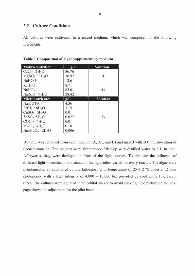
6
22 Culture Conditions
All cultures were cultivated in a mixed medium which was composed of the following
ingredients
Table 1 Composition of algae supplementary medium
Makro Nutrition gL Solution CaCl2 2H2O 3676
A MgSO4 7 H2O 3697 NaHCO3 126 K2HPO3 871
A1 NaNO3 8501 Na2SiO 9H2O 2842 Micronutrientes gL Solution Na2EDTA 436
B
FeCl3 6H2O 315 CuSO4 5H2O 001 ZnSO4 5H2O 0022 COCl2 6H2O MnCl2 4H2O Na2MoO4 2H2O
001 018 0006
105 mL was removed from each medium (A A1 and B) and mixed with 200 mL inoculum of
Scenedesmus sp The reactors were furthermore filled up with distilled water to 2 L in total
Afterwards they were deployed in front of the light sources To simulate the influence of
different light intensities the distance to the light tubes varied for every reactor The algae were
maintained in an automated culture laboratory with temperature of 25 plusmn 2 under a 12 hour
photoperiod with a light intensity of 4000 ndash 10000 lux provided by cool white fluorescent
tubes The cultures were agitated in an orbital shaker to avoid sticking The picture on the next
page shows the adjustment for the pilot batch
7
Figure 1 Pilot batch deployment
The batches were daily readjusted because the light intensity changes when the water level
decreases They were always positioned in a way that at the middle height of the liquid the given
light intensities are steady
8
23 Photometry
Measurement of optical radiation fluxes (light intensities) was performed with use of a
photometer A distinction is made in the analysis between the measurement of absorption
scattering (scattered light) and the fluorescence in liquids and gases
231 Lambert-Beer law
The Lambert-Beer law is considered the fundamental law of absorptiometry It applies to all
optical methods of analytical chemistry Therefore it is based on measuring the absorption of
radiation in the ultraviolet and visible regions of the spectrum Two laws are combined in it The
Beers law which says that the light absorption of a colored solution is proportional to the
concentration of a substance which is dissolved in a colorless solvent and the Lambert law in
which the light absorption of a solution is proportional to the way the light travels through the
sample (at constant concentration of the solute)
A ndash Absorption (excitation)
I0 ndash intensity of emitted light
I ndash intensity of attenuated light
ndash Transmission
c ndash Concentration of sample
d ndash Distance of the light or sample diameter [cm]
ε1 ndash molar absorption coefficient
The equations shows that the absorbance is nothing else than the common logarithm of the
quotient of emitted and detected light The relationship between absorbance and transmission is
shown on the next page 1 This is a specific size in case of the absorbing substance may vary on the pH or the solvent dependent
9
Figure 2 Relation between transmittance and absorbance (httpteachingshuacuk 2014)
The Law states that the fraction of the light absorbed by each layer of solution is the same which
leads to a linear function instead of a logarithmic function by using the Absorbance In terms of
analysis it is easier to have linear function This is why the effect is mainly displayed as a
function of absorbance
Usually the scattering and luminescence effects in the spectroscopy analysis are neglected
Therefore in this work the term absorbance is used (when not specified otherwise) since
extinction is the sum of the effects of absorption scattering and luminescence (Mills Cvitaš
Homann Kallay amp Kuchitsu 1993)
The law applies only under certain conditions Firstly the dissolved substance must be
homogeneously distributed in the cuvette Furthermore it should be noted that the law does not
apply for open-end concentrations This means there is a limit to the concentration that is
measurable After a certain point the absorbance no longer increases in a linear fashion caused
by an over concentration of molecules in the solution In this case light rays can no longer pass
through the medium and correspondingly it is necessary to dilute the sample
10
232 Photometer
A Photometer is in a broad sense a device that is used in biology medicine physics and
chemistry for measuring the light absorption especially for the determination of concentrations
of known substances The main approach is to illuminate a sample and to measure the resulting
light intensity with a detector Different measurement methods are used The following figure
shows the principle of the basic process with one light beam using the example of absorption
measurement
The light source (L) emits a light beam through the medium to be measured in the measuring cell
(M) and the photodetector (Ph) measures the intensity of the remaining light In the amplifier
(V) the electric signal is amplified and output as a measured value
The light source can be a tungsten mercury cadmium H2 or a D2 lamp depending on the used
spectrum Tungsten lamps for example are used in the visible wavelength range and mercury and
cadmium light sources in the ultraviolet wavelength region (wwwphotometercom 2014)
Figure 3 Structure of a photometer (wwwphotometercom 2014)
11
233 Spectrophotometer
Table 2 Specifications of the used T80 spectrophotometer
Double-beam optical system Instrument Type T80 Spectral Bandwidth 2 nm (fixed slit)
Working Mode MPU ModePC Mode
Software Support MPU Software PlatformSpec UV software workstation
Wavelength Range 190 - 1100nm Wavelength Accuracy plusmn 03nm (Automatic wavelength correction) Wavelength Reproducibility 02 nm Stray Light lt 012T (220nm Nal 340nm NaNo2)
Photometric Mode Transmittance Absorbance Energy
Photometric Range -03 - 3Abs
Photometric Accuracy
plusmn 0002 Abs (0 - 05A) plusmn 0004 Abs (05 - 1A) plusmn 03 T (0 - 100 T)
Photometric Reproducibility 0002 Abs (05 - 1A) 015 T (0 ndash 100 T )
Baseline Flatness plusmn 00015 Abs (190 - 1100nm) Baseline Stability 00008 Absh (500nm0Abs 2nm Spectral
Bandwidth 2hr warm-up_ Spectral Bandwidth 2nm (fixed slit) Photometric Noise plusmn 0001 Abs (500nm 0Abs 2nmSpectral
Bandwidth)
In the case of the spectrophotometer white light is decomposed by a prism or a diffraction
grating so that only light with a specific wavelength can pass through a shutter and into the
sample solution With lenses and apertures a narrowly defined light beam is produced consisting
of parallel rays By using filters or monochromators the spectrum of the light is reduced to a
limited wavelength range
While the light passes through the sample a part of the incident light is absorbed by the
molecules in the solution causing a weakening of the light intensity which can be recognized by
the photo detector and the attenuation of light is calculated by a computer (Lehmann 1892)
12
The light attenuation is a measurement of the absorption of light and is therefore a measurement
of the concentration of the absorbing molecules in the analyzed solution In this way the
concentration of the substance can be determined using the Lambert-Beer law or a calibration
curve (Boumlcker 1979)
The final aim of the measurement is the detection of the attenuation of the light intensity by the
substance in the measuring cell The measurement result depends on the brightness of the light
source (L) and the sensitivity of the photodetector (Ph) However the properties of these
components change under the influence of fluctuations in the supply voltage temperature and
aging The single-beam therefore is not stable in the long run and must be frequently
recalibrated (wwwphotometercom 2014)
This may be justifiable for individual measurements in the laboratory but in the context of
industrial settings continuous measurement influences of the light source fluctuations have to be
eliminated This leads to the dual-beam method
Figure 4 Structure of a photometer with a dual-bean (wwwphotometercom 2014)
Here a semi-transparent mirror splits the ray into two beams a measurement beam (M) which
passes through the sample and impinges on a first photodetector and a reference beam (V) which
falls directly on a second receiver
The measured value is created by forming a ratio so that the variations in the luminosity of the
light source have no effect However a remaining error source is the change in the sensitivity of
the two photodetectors Therefore the optimum solution is to use two beams and only one
photoreceptor During the project an UVVIS Spectrophomater (model T80 from PG Insturments
Ltd) was used which works exactly in the described manner
13
Figure 5 Dual beam measuring method with only one photodetector (wwwphotometercom 2014)
Again the measured value is created by calculating the ratio of the sample and reference beams
Due to a rotating disc profile (Chopper) the two beams alternate on the same photo detector This
eliminates not only the variations in the light source but also changes of sensitivity of the
photoreceptor are eliminated (Spektrum 1999)
24 Fluorimeter
Table 3 Specifications of the used FluoroMaxR Fluorimeter
FluoroMaxR-4 with USB von HORIBA Lamp Vertically mounted CW 150 W Ozone-free xenon
arc lamp Gratings 1200 groovemm blazed at 330 nm (excitation) and
500 nm (emission) plane ruled Detectors Emission R928P photon counting PMT (185-850
nm) and reference photodiode for monitoring lamp output
Water Raman SN 60001 (RMS method) See Signal-to-noise ratio Slits Continuously variable from 0 to 30 nm Accuracy 05 nm Repeatability 01 nm Minimum step 00525 nm Integration time 0001 to 160 sec Software FluorEssence Monochromators Automatic self-calibration of all wavelength drives
and slits All reflective optics Czerny-Turner spectrometers
Spectral Correction Factors Included
14
Fluorometry is a molecule-spectroscopic analysis that utilizes the property of electronically
excited molecules to emit the absorbed excitation energy as luminescence radiation Since the
electronic excitation of the molecules take place by absorption of light fluorimetry is a
photoluminecense method It finds versatile applications in both organic and inorganic analysis
The outstanding features of this method are their high selectivity and high sensitivity (Zander
1981)
The process is characterized particularly by some features At first it is a direct photometric
method for qualitative and quantitative analysis It is highly sensitive and has a wide range of
linearity Furthermore there are small amounts of material required for the analysis Online as
well as in-situ analysis are possible Lastly there is no or little sample preparations required
which leads to a non-destructive procedure That means the sample can be returned without
problems (Zander 1981)
Fluorimetry is generally based on the detection of emitted luminescent radiation from a sample
or a photochemical mediator molecule (fluorescent marker)
Luminescence radiation arises when electrons move from a higher to a lower orbital This is
called Stokes shift Stokes fluorescence is the re-emission of longer wavelength photons (lower
frequency or energy) by a molecule that has absorbed photons of shorter wavelengths (higher
frequency or energy) It is characteristic for every substance (Schmidt 2000)
A prevention of fluorescence by other types of dissipation of the excitation energy may occur
For instance an energy transfer to other molecules without radiation (eg photosynthesis) or
internal conversion
The intensity of the fluorescence of a solution depends on the intensity of the excitation light
(Iα) the molar absorption coefficient ε of the fluorescent substance the concentration c of the
sample and the quantum yield Q
I0 ndash intensity of emitted light
Ia ndash intensity of attenuated light
15
c ndash Concentration of sample
d ndash Distance of the light or sample diameter
ε ndash molar absorption coefficient
Fluorimetry is used especially often in the field of quantitative analysis because in this case the
detection sensitivity is much higher than for pure absorption photometry The reason is the ratio
of the absorption photometry where usually slightly different signals are measured (Boumlcker
1979)
The majority of chemical compounds have a fluorescence ability Almost all aromatic
hydrocarbons are characterized by fluorescence assets Nevertheless the introduction of
substituents derogates this Particularly nitro and carboxylic acid as well SH-groups and related
substituents almost completely delate the fluorescence (Schmidt 2000)
Fluorimetry has a high detection limit of 10-12 Mol whereas in the absorption analysis only up
to 10-8 Mol can be detected At high substrate concentrations attention should be paid to the fact
that the fluorescence intensity Q is no longer a linear function of the concentration c To stay in
the linear range a maximum concentration of should not be exceeded In the following
figure the structure of a fluorimeter device is presented
Figure 6 Common structure of a fluorimeter device (Rouilly 2014)
16
Mercury or xenon lamps are often used as sources of excitation light Mercury vapor lamps emit
a line spectrum with high intensities in the lines (at 254 313 36566 405 546 577 630 nm )
via a low-intensity continuous background Xenon lamps have a continuous emission spectrum
but its intensity decreases in the UV range
Important properties of monochromators are their light intensity the spectral slit width and the
freedom of scattered light In modern appliances imaging holographic gratings are used All
optical elements such as lenses gratings mirrors and beam splitters influenced by their spectral
characteristics influence the intensity and polarization of the reflected and transmitted radiation
as a function of wavelength
Photomultiplier are used as which allow due to their high amplification (106 to 108) the
measuring of lower light intensities up to single photons Depending on the material of the
photocathode different types of photoreceptors can vary in terms of their absolute and spectral
sensitivities The gain of the photomultiplier depends on the applied voltage (Zander 1981)
25 Prototype
The instrument which was used for this project was designed to measure and analyze samples of
microalgae by using the method of a fluorimeter In line with the idea of inexpensive production
the construction is relatively basic A schematic diagram is presented in the graphic below
Figure 7 schematic diagram of the prototype sensor (left) and photo (right) (Rolim Heinen amp Huff 2014)
17
As is shown above the installation is similar to the fluorimeter (qv figure 6) The main
components are an LED light source which sends a light beam into an opaque chamber where
the sample is placed and two optical receptors which are positioned at angles of 180deg and 90deg
In contrast to the fluorimeter only one filter is used here (in the fluorimeter three mochrometers
were used) The filter works in the same manner as the monochrometer and blocks all unwanted
wavelengths so that just one specific or particular spectrum can pass through
Figure 8 Filter ldquoStrawrdquo to eliminate unwished wave length
The filter absorbs undesired wavelengths between 300 and 400 nm but has a transmission of 88
in case of the important spectrum (lt 400 nm) which is not optimal but a calculable factor
since itrsquos the same loss in any sample and series of tests
Even though lasers have excellent characteristics in case of accuracy and wavelength they are
relatively expensive In opposition to LEDs In opposition to LEDs Caused by that an LED light
source is installed together with the two optical sensors The high potency LED lamp emits a
blue light beam which fits well with the potential spectrum of absorbance of the chlorophyll and
should provide optimal requirements for the microalgae
18
26 Measurement of Biomass
The analyses of the biomass provides information about growth rate and as a consequence
thereof biological activity Therefore a vacuum pressure pump was used together with paper
filters with a diameter of 205 μm and a pore size of 14 μm
A sample of 50 ml was taken from the batches and filtered through the paper (weighted before)
while the vacuum pump supported the passaging of the liquid Afterwards the nearly-dry paper
was stored in an oven at 60 degC for approximately 24 hours The mass difference gives some
indication of the amount of biomass in the 50 ml solution
27 Measurement of Chlorophyll
An issue in chlorophyll measurement is extracting the pigments from the cells Therefore a
sample of 10 ml is filtered (same procedure as for biomass) The extract is stored afterwards in a
90 acetone solution at 4 degC for approximately 24 hours Acetone is a moderate polar solvent
which is after methanol the best solution for chlorophyll pigments because it consists of polar
areas as well as a lipophilic phytel rest (see figure 9) (Lourenccedilo 2006)
Figure 9 Chemical structure of chlorophyll (Willows 2013)
19
Due to the reference (Lourenccedilo 2006) the solution should be centrifuged for around 10 minutes
and 3000 rpm This strategy is used because usually the filter is cut in pieces before stored in the
tube to guarantee a better detachment of the chlorophyll The pre-tests have shown that the
results are more accurate when the filter isnrsquot cut but rolled up and put into the tube (filtrate
towards the tubes inside) If than filled carefully up with acetone (washing out of the extract
must be avoided during infusion) the extraction of chlorophyll will be optimal without the
problem of filter rests and other cell bodies
In a further step the chlorophyllacetone solution is measured in a spectrophotometer by 630 nm
647 nm and 663 - 665 nm The amount of chlorophyll is calculated by the following statistic
equations from Lourenccedilo (2006)
D663-665 D647 D630 ndash absorbance at the wavelength Dx after correction by the cell-to-cell blank and subtraction of the cell-to-cell blank corrected absorbance at 750nm
l - Cell (cuvette) length [cm] = 1
v - Volume of acetone [ml] = 10
V - Volume of filtered water [l] = 10
Accordingly the term That simplifies the equations
20
3 Results and discussion
During the project the algae suspension was scanned over a time interval of 10 days plus one
day incubation During this time the batches were subjected to various light conditions (Batch A
= 4000 Lux Batch B = 5500 Lux Batch C = 7000 Lux Batch D = 8500 Lux Batch E = 10000
Lux) This was performed to analyze the effect of different light intensity on algae and
accumulation of chlorophyll To obtain useful results it is essential to eliminate as much
unwished problems as possible According to this the growing of the algae was analyzed at first
because any discrepancies of the algae growth would lead to consequential errors in case of
chlorophyll tests
31 Algae growth The growth of Scanedesmus Sp was measured via spectrophotometer and biomass dry weight
Optical density of biomass was determined at 750 nm One ml of the sample batch was taken and
measured in a spectrum between 400 nm and 750 nm
Usually the growth of an algae culture follows certain steps It starts with the lag phase (1)
followed by an exponential phase (2) The culture growth will reach a point of overpopulation in
which one or more essential resources are limited Growth and death rate are either in
equilibrium or the cells already stopped the proliferation This is called the stationary phase (4)
At the end the living conditions are so bad that the cell population starts to decrease rapidly
(usually caused by a deficiency of important nutrients) The last phase is called death phase (5)
Figure 10 Sketch of algae growth dynamics
21
The before explained growth dynamic differs to the culture development during the test Figure 7
(below) presents all graphs (of absorbance [400hellip750 nm]) of the five batches in a time interval
of ten days So in total 50 single graphs summarized in that 3D - graphic It gives an interesting
overview of the total experiment
Figure 11 Progress of all 5 batches in a time interval of 11 days
In the figure a formation can be seen that looks like one side of a steep ridge that starts relatively
flat in the beginning and becomes steeper in the posterior tier Rifts in the formation are caused
by some problems associated with the spectrophotometer at certain wavelengths Following the
observation that the results are the same regardless of the kind of sample analyzed the
assumption that the spectrophotometer doesnrsquot work at these wave length may be accepted
Furthermore a pattern of wave formations is recognizable Every wave formation has a
maximum at around 400 nm and 480 nm and between 650 nm and 670 nm The first ldquowaverdquo is
the result of the batch analyses from the first day the second from the second day and so on
The wavelike formation is caused by the differential growth of the algae under different light
22
conditions The most exposed batch (E) already has a higher algae concentration on dayx as
compared to the lowest exposed batch (A) one day after
Figure 12 By comparison absorbance between 400 nm and 750 nm of five batches at day 6 and 72
The first figure curvebatch E has the highest absorbance starting between 06 and 065 at 400
nm and ending up at the second maximum at around 059 In comparison batchcurve A from
one day after also starts between 06 and 065 but falls under the values of Batch E at the second
maximum which occurs at around 056 This is responsible for the wave effect between the
days Only at the last day does Batch A exceed the high peaks of Batch E from the previous day
This is caused by the beginning of the exponential phase Unfortunately the cultures did not pass
through all four phases as expected The exponential phase started between day 7 and 9
depending on the Batch
2 The days are chosen randomly to proof the above delineated statement The same course of curves could be confirmed for every day Just the intensity of absorbance varies
23
We can see the effect of light between the different figures The culture of Batch E already began
exponential growth at day 7 while the lag phase in Batch A persisted until the 8th9th day
Figure 13 Progress of culture growth comparing Batch E (left) and A (right) during the 10 days in comparison to the Absorbance
The following statements can be made to summarize the observed algae growth Since the
different colonies in the Batches react to the light intensity as expected the assertion can be
made that the Biomass (mB) of
When comparing the results of the optical density with the gravimetric measurements some
issues have to be mentioned The dry weight measurement was only performed after day four
because the amount of biomass measured before day five was considered too small to be reliably
assessed Even after the fifth day some unexpected changes in the curve shape were visible
Nonetheless the main shape of the curve approximates an exponential slope after day eight
which is consistent with the measurement of the optical density
24
Figure 14 Dry weight (mgl) of Scenedesmus Sp for 10 days grown under different light conditions
In addition the amount of biomass increases daily in every Batch according to the results of the
optical density
This is not so in the case of the dry weight measurement where no decipherable pattern can be
determined for the first half of the test period Some problems occurred during the laboratory
processing including the malfunctioning of an oven during day 6 and a restoration of the
samples during day seven Additionally as a consequence of the high error-proneness of the
earlier dry weight analysis due to the use of relatively small volumes findings from the dry
weight analyses should be considered with caution
Beyond these issues it has to be mentioned that the colonies didnrsquot reach the stationary phase
and thus also failed reach the death phase These two statuses of the growth dynamic could
have been interesting for the comparison of the algaechlorophyll ratio while exposed to different
light intensities
25
The results of biomass and spectrophotometer analyses confirm the findings of the designed
prototype in the way that the order of the batches in proportion to dissolved substances (
biomass) is the same as the order of the Batches themselves (BA lt BB lt BC lt BD lt BE dayx)
Figure 15 Algae development measured by prototype during the days 7 - 11 plotted as a function of voltage
The figure above shows the general light intensity that passes through the sample filled with
water (~ 245 V) The larger the amount of dissolved material in the sample the less light will
pass through it and consequently the lower the measured voltage will be With a general
tendency toward a lower voltage a larger amount of biomass can be ascertained but it has to be
mentioned that no statements about the type of curve shape can be made Unfortunately more
test results would have been necessary to make further statements
0
05
1
15
2
25
3
7 8 9 10 11
Outp
ut vo
ltage
at 1
80deg(
V)
Days
A
B
C
D
E
Water
26
32 Chlorophyll formation
After the chlorophyll-acetone mix is stored for 24 hours it is analyzed with a spectrophotometer
For the calculation of chlorophyll content according to Jeffrey amp Humphrey (1975) only some
wavelengths are important Nevertheless the chlorophyll was treated in the same way as the
algae and measurements were made in the range of 400 nm to 750 nm in order to determine
possible similarities
Figure 16 Chlorophyll (mgl) of Scenedesmus sp for 10 days grown under different illumination conditions
The concentration of total chlorophyll increases during the test The results show a steady growth
if expressed as the exponential regression curve (dotted lines) for Batches D and E (R = 09) A
better correlation is shown for a linear regression for Batches A and B (R = 09 instead of 076)
Batch C doesnrsquot show a strong correlation under either a linear (R = 072) or an exponential
growth (R = 076) assumption Many factors affect the results of the Chlorophyll measurement
Firstly the analyses are susceptible to mistakes made during the processing When removing 10
ml from the batches with a concentration of barely 1 mgL and using those samples in a cuvette
of 3 mL the amount of Chlorophyll is typically in a range of 0 ndash 10 μgmL Working with such
small quantities can lead to inaccuracies during processing in addition to errors made on behalf
of the measuring engine itself
Rsup2 = 07602
Rsup2 = 07602
Rsup2 = 09004
Rsup2 = 09037
Rsup2 = 07594
0
05
1
15
2
25
0 1 2 3 4 5 6 7 8 9 10 11
Chlo
roph
yll a
+b (m
gl)
Day
C
D
E
B
A
Expon (C)
Expon (C)
Expon (C)
Expon (D)
Expon (D)
Expon (E)
Linear (B)
Expon (A)
Linear (A)
27
Nevertheless we can make the assumption that the tendency (daily increase) makes sense The
results of the pilot engine show slightly decreasing curves At day 8 there is an obvious mistake
to declare This is not visible with regard to algae measurement at day 93 This leads to the
assumption of a mistake made during the preparing procedure with acetone Since the
abnormality can be found in all batches a mistake during the withdrawal can be ruled out
Figure 17 Chlorophyll development during the days 7 - 11 plotted as a function of voltage
A further problem is that the curves are not clearly separable They cross each other without
showing a decipherable trend with regard to which batch has the highest or the lowest
translucency (which would be proportional to the voltage) As a consequence these results
cannot provide information about the effect of different light irradiation and it is questionable
whether they can be used to make an assumption about chlorophyll accumulation
3 The spectrophotometer analyzes of chlorophyll is one day after due to the 24 hours storing of the samples
0
05
1
15
2
25
3
7 8 9 10 11
Outp
ut vo
ltage
at 1
80deg(
V)
Days
E
B
C
D
A
Water
28
33 Correlation of Algae and Chlorophyll growth The main rationale for using different light irradiation for the Batches was to determine the
relationship between algae growth and the Chlorophyll enhancement Hence interest lay beyond
simply examining the thesis that the concentration of Chlorophyll is directly linked to the algae
growth Furthermore there was interest in exploring whether a specific relationship existed
between the algae growth rate the exposure to light and the amount of chlorophyll produced
Figure 18 Collocation of AlgaeChlorophyll absorbance (by 665 nm) by a spectrophotometer for 11 days
Unfortunately an incomplete test phase (no algae growth until the stationary phase) was
responsible for a lack of results that could be used for further analysis Nevertheless the ratio of
Chlorophyll-to-Algae growth shows a decent progression (see also Table 4) There is no
evidence for a similar progression if the tests proceed for one or two weeks In theory the
chlorophyll concentration should increase more rapidly in the exponential phase (until now the
progress is best described as a linear growth) Furthermore the concentration of algae as well as
of chlorophyll from batch E should reach its maximum first followed by batch D C B A (in
this order) and continue at a stationary rate
BAA
lgae
BAC
hlBB
Alg
aeBB
Chl
BCA
lgae
BCC
hl
BDA
lgae
BDC
hl
BEA
lgae
BEC
hl
002040608
112141618
12
34
56
78
9 1011
BatchSubstrate
Abso
rban
ce
Days
BAAlgae
BAChl
BBAlgae
BBChl
BCAlgae
BCChl
BDAlgae
BDChl
BEAlgae
BEChl
29
Due to the issues described in the earlier chapters the results from analyses on biomass are less
convincing than those arising from the analyses of the spectrophotometer In addition and
contrary to the absorbance measurement the values of dry weight and calculated chlorophyll
correlate weakly in cases of batches with higher light saturation This may be due to inaccuracies
from the dry weight results or another reason could be the earlier start of a kind of exponential
growth for the chlorophyll while the results for the biomass donrsquot show an exponential increase
until the 7th day
Table 4 Overview of the results of biomass prototype and spectrophotometer analyzes
Substrate Biomass (mgl) ndash Dry weight and Chl Optical density (V) -
Prototype Absorbance - Spectrophotometer
Min Max R Min Max R Min Max R BAAlgae 146 327
092 185 061
- 013 156
094 BAChl 001 164 212 170 001 017 BBAlgae 154 444
085 124 049
- 013 169
089 BBChl 004 172 206 175 001 026 BCAlgae 170 478
078 097 042
- 012 170
082 BCChl 002 188 194 181 001 023 BDAlgae 162 504
068 104 044
- 011 172
094 BDChl 002 124 196 171 001 026 BEAlgae 160 515
066 130 035
- 009 175
097 BEChl 002 114 215 195 001 031 The less exciting results are unfortunately given by the Prototype Here no significant correlation
can be mentioned at all In contrast to the spectrophotometer these values are provided by the
direct transmission Therefore the highest solution has the lowest value because more light is
absorbed by the dissolved material which is in this case biomass (or pure chlorophyll) This
result is surprisingly disappointing because the tests performed beforehand with fluorescence
(realized by Leonardo M Rolim) show a straight dependency of proportional relationship
between percental solution and transmission (see Figure 19 below)
Fluorescein is a fluorescent dye from the group of the xanthene It was used for the previous tests
because itrsquos a non-biological and well known substance with which all unwished side effects of a
living system can be avoided during tests
30
Figure 19 Measuring points of concentration given in optical density from fluorescence (Rolim Heinen amp Huff 2014)
The graph shows the transmission by 180 degC as accomplished with the algae and chlorophyll
during this work The curve suggests a negative exponential trend This was also expected for the
new series of tests While a clear difference can be recorded in the case of fluorescein the values
of chlorophyll almost didnrsquot change This could be an effect of the high fluorescent impact of
fluorescence Due to the growth rate of chlorophyll (see Table 4 Chl Min and Max) which goes
from 001 gmL up to almost 18 gmL (180 times more) compared with the fluorescence which
goes from 001 gmL up to 03 gmL (30 times more) this is questionable since the concentration
difference is 5 times higher for pure chlorophyll a fluorescent pigment as well but the effect is
very little Nevertheless it could be an indication as to why results from the test were not as
expected
The analyses by the fluorimeter provides further interesting results The figure below presents
the results of chlorophyll for the 11th day The x-axis shows the input of the wave length
produced by the laser The excitation is visible on the y-axis while curves on the graph present
one specific wave length each between 400 and 800 nm (with an interval of 5 ie a new
measurement was performed for every 5 nm) In order to simplify the graphical presentation the
legend was omitted
31
Figure 20 Display of emission and excitation measured by the fluorimeter of day 11 for chlorophyll
The figure provides an important insight into the behavior of chlorophyll fluorescent The
formation on the bluish part of the light spectrum (270 ndash 430 nm) and the second cluster of peaks
between 650 and 675 nm are quite revealing The table below explains the most important
curves
Table 5 Legend of figure 16
Color wave length (nm) red 675 blue 670 gray 680
light green 665 orange 685
light blue 660 dark blue 690 dark green 695
These eight curves are explicitly mentioned because they have the highest response in the tested
emission spectrum Due to usually low concentrations of samples eg chlorophyll in μgml a
high response is vital The results of the other test days are equal They simply vary in the height
of excitation as a result of a higher concentration
0
200000
400000
600000
800000
1000000
1200000
1400000
1600000
300 325 350 375 400 425 450 475 500 525 550 575 600 625 650 675 700 725 750
Exita
tion
ampe
rage
at 9
0deg(m
A)
Emission wave lenght (nm)
32
Figure 21 Display of emission and excitation measured by the fluorimeter between the days 0 and 11 for chlorophyll (BA)
The daily difference of the excitation is presented above The course of the curves is equal and
just differs as mentioned before in the amount of ampere measured by the receptor The same
shape would be plotted by the other batches The only difference again would be the level of
excitation
The progression of the chlorophyll curves during the tests shows a permanent increase beginning
at day three An exponential correlation can be verified for the plotted curves Thus the results
from the fluorimeter are as expected before Still the problem as mentioned before of the
incomplete growth of the algae was responsible for a lack of further information which could
have been interesting
0
200000
400000
600000
800000
1000000
1200000
350 375 400 425 450 475 500 525 550 575 600 625 650 675 700 725 750
Excit
atio
n am
pera
ge a
t 90
deg(m
A)
Emission wave lenght (nm)
0
1
2
3
4
5
6
7
8
9
10
11
33
Figure 22 Trend of the chlorophyll excitation peaks during 11 days measured by the fluorimeter
In the following section the results from the algae analyses are explained One problem has to be
mentioned beforehand
The graph below shows the outcome from the last day Highly overlapping curves are visible
This is not caused by fluorescence but by the reflection of each wave length itself due to a high
solution The analyses made by the fluorimeter requires at least 30 minutes That it enough time
for the dissolved particle to settle down The x-axis can accordingly be viewed as a timeline
scale As more time passes by the reflection impact reduces
Rsup2 = 08453
0
200000
400000
600000
800000
1000000
1200000
1400000
1600000
1800000
2000000
0 2 4 6 8 10 12
Excit
atio
n am
pera
ge a
t 90
deg(m
A)
Days
660
665
430
405
375
Log (375)
34
Figure 23 Fluorimeter results of algae (BA day11)4
When the y-axis is limited to 100000 mA some other formations are visible Interestingly they
have the same shape as the curves of the chlorophyll which leads to the assumption that those
overlapped curves are indeed the fluorescent impact of the chlorophyll pigments
4 Every curve presents one wave length of the emission spectrum in an interval of five The legend is once more excluded due to a better overview
0
1000000
2000000
3000000
4000000
5000000
6000000
7000000
8000000
300 325 350 375 400 425 450 475 500 525 550 575 600 625 650 675 700 725 750
Excit
atio
n am
pera
ge a
t 90deg
(mA)
Emission wave lenght (nm)
35
Figure 24 Fluorimeter results of algae (BA day11) with limited y-axes up to 100000 mA5
On closer examination it can be interpreted that the higher curves (blue orange green dark
blue redhellip) are the same wavelengths as seen in the Table 5 Legend of figure 16rdquo The highest
response again is at 675 nm Measureing by a different wave length than 675 nm will cause
lower excitation The same happens in case of chlorophyll
The excitation is low in comparison with the results of the pure chlorophyll because the
chlorophyll is not separated from the cells which hinders the light from reaching the pigments
in addition to leaving the sample and stimulating the receptor
The comparison with the other batches and the analyses of the different days provides the same
results as for the chlorophyll That means the Excitation of BA(dx) lt BB(dx) lt BC(dx) lt BD(dx)
lt BE(dx) and the Excitation of BA(dx) lt BA(dx+1) BB(dx) lt BB(dx+1) BC(dx) lt BC(dx+1)
BD(dx) lt BD(dx+1) BE(dx) lt BE(dx+1)
5 The legend is once more excluded due to a better overview
0
10000
20000
30000
40000
50000
60000
70000
80000
90000
100000
300 325 350 375 400 425 450 475 500 525 550 575 600 625 650 675 700 725 750
Excit
atio
n am
pera
ge a
t 90
deg(m
A)
Emission wave lenght (nm)
36
4 Conclusiones
According to the results from the fluorimeter the algae growth and chlorophyll enhancement
appear to be as expected This leads to the question as to why the previous tests donrsquot have
similar outcomes The answer to this question and the reason why fluorimeters are used for low
quantities is the same They have a very high accuracy and are thus extremely efficient even
for low quantities Nevertheless they are extremely expensive and the main task of this project
was to determine whether it was possible to measure chlorophyll (pure or even intracellular) with
the prototype or if not to work out further steps for the development of the engine
The first step apart from the biological section is to make the engine more stable During the
project problems often occurred with regard to replication of results because small changes in the
electrical connection contributed to different outcomes while using the same sample This made
the testing more complicated and made unnecessary repetitions of measurement indispensable A
shell for the entire construction in which the electronic is fixed should solve this problem An
extension cable which leads to the measuring box together with a smaller diameter of the cell
itself would also be useful The laser and the two receptors should be installed separately from
the cell and waterproofed (plastic and glue should be sufficient) As a result the cell could be
introduced into a sample to measure which not only simplifies the procedure but it is also closer
to any practical application
The next action is the acquisition of the correct optical filter The results of the fluorimeter
suggest an optimal emission at 430 plusmn 10 nm while the excitation should be measured at 675 plusmn 10
nm The closer the measurement is to these wavelengths the higher the values of the results
Furthermore it was explained how other wave lengths overlap the fluorescence effect This can
be avoided by use of at least two filters one which filters the light of the laser and blocks out
every wavelength except for those in the range of eg 420 ndash 440 nm and a second filter which
allows for only the spectrum from 665 to 685 nm to pass
Nevertheless an upgrade of either the receptor or laser but probably both will be inevitable As
mentioned in the previous chapter the outcome of the 90deg measurement for algae and
chlorophyll is almost zero In actuality it has the same value as if measured with water which
means that the receptor is not able to recognize any approaching light On the other hand it may
37
be that the laser is too weak so that not enough light is injected In any case adjustment for the
right filter range should be the first step
When the filter and laserreceptor problems are solved a new test with fluorescence would make
sense At this stage it is important not only that the results are good for one series of tests but
also that they are repeatable Daily calibration of the engine is not only effortful and time-
consuming but it can also lead to variable results After good and stable results are achieved
with fluoresce a new test series with algae can be started Therefore it would be useful to create
a serial dilution of an algae culture which is already in the stationary phase and highly
concentrated If the results are suitable it can be continued with a serial dilution of those algae
Even if the results from the 90deg measurement are not satisfying a further test with pure
chlorophyll could be accomplished on condition that the results from the 180deg measurement are
decent
Only after all the described experiments have sufficient results should a new long-term test series
be started For this purpose no more than three batches should be installed with an intensity of
illumination between 3000 and 10000 lux The test duration should be approximately 30 days to
ensure that the culture passes through all growing and dying phases Tests performed with the
spectrophotometer can indicate a change of the growing conditions so that further and more
elaborated tests with the fluorimeter and biomass can be performed The measurement of
biomass should be sufficient if performed every three days (a daily testing during the exponential
phase would perhaps be useful) By using the fluorimeter care has to be taken so that the dilution
of the sample is large enough otherwise overlapping effects occur The analyses with the sensor
should be performed daily in order to get a consistent overview of the chlorophyllalgae ratio as
well as to gauge the accuracy of the sensor
38
5 Bibliography Boumlcker J (1979) Spektroskopie Instrumentelle Analytik mit Atom- und Molekuumllspektroskopie
(1 Edition Ausg) Wuumlrzburg Vogel Verlag und Druck GmbH amp Co
Hegewald P (2006) Scenedesmusndashlike algae of Ukraine Tsarenko E amp B Braband
Lehmann E W (1892) Uumlber ein Photometer Erlangen
Lourenccedilo S (2006) Cultivo de Microalgas Marinhas Princiacutepios e Aplicaccedilotildees
Luumlrling M (1999) The Smell of Water Grazer-Induced Colony Formation in Scenedesmus
Wageningen Pulz und Gross
Mills I Cvitaš T Homann K Kallay N amp Kuchitsu K (1993) Quantities Units and
Symbols in Physical Chemistry (Green Book)
Rolim L M Heinen A L amp Huff D D (2014) Desenvolvimento de sensor oacuteptico portaacutetil
para mediccedilatildeoes online de concentraccedilatildeo no cultivo de microalgas Porto Alegre
Rouilly V (2014) Schmidt W (2000) Optische Spektroskopie (Bd 2 Edition) Weinheim
WILEY-VCH Verlag GmbH
Unknown (1999) Photometer Spektrum Akademischer Verlag
Willows R D (2013) Structure of chlorophyll Organic Letters
Zander M (1981) Fluorimetrie Berlin-Heidelberg-New York Springer-Verlag
Internet sources Openwetwareorg
photometercom
teachingshuacuk
wikipediaorg
39
6 List of figures Figure 1 Pilot batch deployment 7
Figure 2 Relation between transmittance and absorbance 9
Figure 3 Structure of a photometer 10
Figure 4 Structure of a photometer with a dual-bean 12
Figure 5 Dual beam measuring method with only one photodetector 13
Figure 6 Common structure of a fluorimeter device 15
Figure 7 schematic diagram of the prototype sensor (left) and photo (right) 16
Figure 8 Filter ldquoStrawrdquo to eliminate unwished wave length 17
Figure 9 Chemical structure of chlorophyll 18
Figure 10 Sketch of algae growth dynamics 20
Figure 11 Progress of all 5 batches in a time interval of 11 days 21
Figure 13 By comparison absorbance between 400 nm and 750 nm of five batches at day 6 and 7
22
Figure 14 Progress of culture growth comparing Batch E (left) and A (right) during the 10 days
in comparison to the Absorbance 23
Figure 15 Dry weight (mgl) of Scenedesmus Sp for 10 days grown under different light
conditions 24
Figure 16 Algae development measured by prototype during the days 7 - 11 plotted as a function
of voltage 25
Figure 17 Chlorophyll (mgl) of Scenedesmus sp for 10 days grown under different illumination
conditions 26
Figure 18 Chlorophyll development during the days 7 - 11 plotted as a function of voltage 27
Figure 19 Collocation of AlgaeChlorophyll absorbance (by 665 nm) by a spectrophotometer for
11 days 28
Figure 20 Measuring points of concentration given in optical density from fluorescence 30
Figure 21 Display of emission and excitation measured by the fluorimeter of day 11 for
chlorophyll 31
Figure 22 Display of emission and excitation measured by the fluorimeter between the days 0
and 11 for chlorophyll (BA) 32
Figure 23 Trend of the chlorophyll excitation peaks during 11 days measured by the fluorimeter
33
Figure 24 Fluorimeter results of algae (BA day11) 34
Figure 25 Fluorimeter results of algae (BA day11) with limited y-axes up to 100000 mA 35
40
7 List of tables Table 1 Composition of algae supplementary medium 6
Table 2 Specifications of the used T80 spectrophotometer 11
Table 3 Specifications of the used FluoroMaxR Fluorimeter 13
Table 4 Overview of the results of biomass prototype and spectrophotometer analyzes 29
Table 5 Legend of figure 16 31
41
Declaration of Authorship I hereby certify that this work has been composed by me and is based on my own work
unless stated otherwise No other person`s work has been used without due
acknowledgement in this report All references and verbatim extracts have been quoted
and all sources of information including graphs and data sets have been specifically
acknowledged
______________________ ________________________ Ort Datum Signature
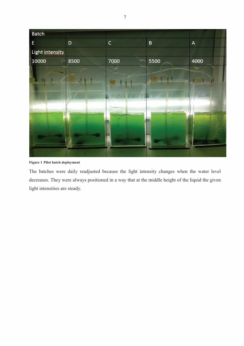
7
Figure 1 Pilot batch deployment
The batches were daily readjusted because the light intensity changes when the water level
decreases They were always positioned in a way that at the middle height of the liquid the given
light intensities are steady
8
23 Photometry
Measurement of optical radiation fluxes (light intensities) was performed with use of a
photometer A distinction is made in the analysis between the measurement of absorption
scattering (scattered light) and the fluorescence in liquids and gases
231 Lambert-Beer law
The Lambert-Beer law is considered the fundamental law of absorptiometry It applies to all
optical methods of analytical chemistry Therefore it is based on measuring the absorption of
radiation in the ultraviolet and visible regions of the spectrum Two laws are combined in it The
Beers law which says that the light absorption of a colored solution is proportional to the
concentration of a substance which is dissolved in a colorless solvent and the Lambert law in
which the light absorption of a solution is proportional to the way the light travels through the
sample (at constant concentration of the solute)
A ndash Absorption (excitation)
I0 ndash intensity of emitted light
I ndash intensity of attenuated light
ndash Transmission
c ndash Concentration of sample
d ndash Distance of the light or sample diameter [cm]
ε1 ndash molar absorption coefficient
The equations shows that the absorbance is nothing else than the common logarithm of the
quotient of emitted and detected light The relationship between absorbance and transmission is
shown on the next page 1 This is a specific size in case of the absorbing substance may vary on the pH or the solvent dependent
9
Figure 2 Relation between transmittance and absorbance (httpteachingshuacuk 2014)
The Law states that the fraction of the light absorbed by each layer of solution is the same which
leads to a linear function instead of a logarithmic function by using the Absorbance In terms of
analysis it is easier to have linear function This is why the effect is mainly displayed as a
function of absorbance
Usually the scattering and luminescence effects in the spectroscopy analysis are neglected
Therefore in this work the term absorbance is used (when not specified otherwise) since
extinction is the sum of the effects of absorption scattering and luminescence (Mills Cvitaš
Homann Kallay amp Kuchitsu 1993)
The law applies only under certain conditions Firstly the dissolved substance must be
homogeneously distributed in the cuvette Furthermore it should be noted that the law does not
apply for open-end concentrations This means there is a limit to the concentration that is
measurable After a certain point the absorbance no longer increases in a linear fashion caused
by an over concentration of molecules in the solution In this case light rays can no longer pass
through the medium and correspondingly it is necessary to dilute the sample
10
232 Photometer
A Photometer is in a broad sense a device that is used in biology medicine physics and
chemistry for measuring the light absorption especially for the determination of concentrations
of known substances The main approach is to illuminate a sample and to measure the resulting
light intensity with a detector Different measurement methods are used The following figure
shows the principle of the basic process with one light beam using the example of absorption
measurement
The light source (L) emits a light beam through the medium to be measured in the measuring cell
(M) and the photodetector (Ph) measures the intensity of the remaining light In the amplifier
(V) the electric signal is amplified and output as a measured value
The light source can be a tungsten mercury cadmium H2 or a D2 lamp depending on the used
spectrum Tungsten lamps for example are used in the visible wavelength range and mercury and
cadmium light sources in the ultraviolet wavelength region (wwwphotometercom 2014)
Figure 3 Structure of a photometer (wwwphotometercom 2014)
11
233 Spectrophotometer
Table 2 Specifications of the used T80 spectrophotometer
Double-beam optical system Instrument Type T80 Spectral Bandwidth 2 nm (fixed slit)
Working Mode MPU ModePC Mode
Software Support MPU Software PlatformSpec UV software workstation
Wavelength Range 190 - 1100nm Wavelength Accuracy plusmn 03nm (Automatic wavelength correction) Wavelength Reproducibility 02 nm Stray Light lt 012T (220nm Nal 340nm NaNo2)
Photometric Mode Transmittance Absorbance Energy
Photometric Range -03 - 3Abs
Photometric Accuracy
plusmn 0002 Abs (0 - 05A) plusmn 0004 Abs (05 - 1A) plusmn 03 T (0 - 100 T)
Photometric Reproducibility 0002 Abs (05 - 1A) 015 T (0 ndash 100 T )
Baseline Flatness plusmn 00015 Abs (190 - 1100nm) Baseline Stability 00008 Absh (500nm0Abs 2nm Spectral
Bandwidth 2hr warm-up_ Spectral Bandwidth 2nm (fixed slit) Photometric Noise plusmn 0001 Abs (500nm 0Abs 2nmSpectral
Bandwidth)
In the case of the spectrophotometer white light is decomposed by a prism or a diffraction
grating so that only light with a specific wavelength can pass through a shutter and into the
sample solution With lenses and apertures a narrowly defined light beam is produced consisting
of parallel rays By using filters or monochromators the spectrum of the light is reduced to a
limited wavelength range
While the light passes through the sample a part of the incident light is absorbed by the
molecules in the solution causing a weakening of the light intensity which can be recognized by
the photo detector and the attenuation of light is calculated by a computer (Lehmann 1892)
12
The light attenuation is a measurement of the absorption of light and is therefore a measurement
of the concentration of the absorbing molecules in the analyzed solution In this way the
concentration of the substance can be determined using the Lambert-Beer law or a calibration
curve (Boumlcker 1979)
The final aim of the measurement is the detection of the attenuation of the light intensity by the
substance in the measuring cell The measurement result depends on the brightness of the light
source (L) and the sensitivity of the photodetector (Ph) However the properties of these
components change under the influence of fluctuations in the supply voltage temperature and
aging The single-beam therefore is not stable in the long run and must be frequently
recalibrated (wwwphotometercom 2014)
This may be justifiable for individual measurements in the laboratory but in the context of
industrial settings continuous measurement influences of the light source fluctuations have to be
eliminated This leads to the dual-beam method
Figure 4 Structure of a photometer with a dual-bean (wwwphotometercom 2014)
Here a semi-transparent mirror splits the ray into two beams a measurement beam (M) which
passes through the sample and impinges on a first photodetector and a reference beam (V) which
falls directly on a second receiver
The measured value is created by forming a ratio so that the variations in the luminosity of the
light source have no effect However a remaining error source is the change in the sensitivity of
the two photodetectors Therefore the optimum solution is to use two beams and only one
photoreceptor During the project an UVVIS Spectrophomater (model T80 from PG Insturments
Ltd) was used which works exactly in the described manner
13
Figure 5 Dual beam measuring method with only one photodetector (wwwphotometercom 2014)
Again the measured value is created by calculating the ratio of the sample and reference beams
Due to a rotating disc profile (Chopper) the two beams alternate on the same photo detector This
eliminates not only the variations in the light source but also changes of sensitivity of the
photoreceptor are eliminated (Spektrum 1999)
24 Fluorimeter
Table 3 Specifications of the used FluoroMaxR Fluorimeter
FluoroMaxR-4 with USB von HORIBA Lamp Vertically mounted CW 150 W Ozone-free xenon
arc lamp Gratings 1200 groovemm blazed at 330 nm (excitation) and
500 nm (emission) plane ruled Detectors Emission R928P photon counting PMT (185-850
nm) and reference photodiode for monitoring lamp output
Water Raman SN 60001 (RMS method) See Signal-to-noise ratio Slits Continuously variable from 0 to 30 nm Accuracy 05 nm Repeatability 01 nm Minimum step 00525 nm Integration time 0001 to 160 sec Software FluorEssence Monochromators Automatic self-calibration of all wavelength drives
and slits All reflective optics Czerny-Turner spectrometers
Spectral Correction Factors Included
14
Fluorometry is a molecule-spectroscopic analysis that utilizes the property of electronically
excited molecules to emit the absorbed excitation energy as luminescence radiation Since the
electronic excitation of the molecules take place by absorption of light fluorimetry is a
photoluminecense method It finds versatile applications in both organic and inorganic analysis
The outstanding features of this method are their high selectivity and high sensitivity (Zander
1981)
The process is characterized particularly by some features At first it is a direct photometric
method for qualitative and quantitative analysis It is highly sensitive and has a wide range of
linearity Furthermore there are small amounts of material required for the analysis Online as
well as in-situ analysis are possible Lastly there is no or little sample preparations required
which leads to a non-destructive procedure That means the sample can be returned without
problems (Zander 1981)
Fluorimetry is generally based on the detection of emitted luminescent radiation from a sample
or a photochemical mediator molecule (fluorescent marker)
Luminescence radiation arises when electrons move from a higher to a lower orbital This is
called Stokes shift Stokes fluorescence is the re-emission of longer wavelength photons (lower
frequency or energy) by a molecule that has absorbed photons of shorter wavelengths (higher
frequency or energy) It is characteristic for every substance (Schmidt 2000)
A prevention of fluorescence by other types of dissipation of the excitation energy may occur
For instance an energy transfer to other molecules without radiation (eg photosynthesis) or
internal conversion
The intensity of the fluorescence of a solution depends on the intensity of the excitation light
(Iα) the molar absorption coefficient ε of the fluorescent substance the concentration c of the
sample and the quantum yield Q
I0 ndash intensity of emitted light
Ia ndash intensity of attenuated light
15
c ndash Concentration of sample
d ndash Distance of the light or sample diameter
ε ndash molar absorption coefficient
Fluorimetry is used especially often in the field of quantitative analysis because in this case the
detection sensitivity is much higher than for pure absorption photometry The reason is the ratio
of the absorption photometry where usually slightly different signals are measured (Boumlcker
1979)
The majority of chemical compounds have a fluorescence ability Almost all aromatic
hydrocarbons are characterized by fluorescence assets Nevertheless the introduction of
substituents derogates this Particularly nitro and carboxylic acid as well SH-groups and related
substituents almost completely delate the fluorescence (Schmidt 2000)
Fluorimetry has a high detection limit of 10-12 Mol whereas in the absorption analysis only up
to 10-8 Mol can be detected At high substrate concentrations attention should be paid to the fact
that the fluorescence intensity Q is no longer a linear function of the concentration c To stay in
the linear range a maximum concentration of should not be exceeded In the following
figure the structure of a fluorimeter device is presented
Figure 6 Common structure of a fluorimeter device (Rouilly 2014)
16
Mercury or xenon lamps are often used as sources of excitation light Mercury vapor lamps emit
a line spectrum with high intensities in the lines (at 254 313 36566 405 546 577 630 nm )
via a low-intensity continuous background Xenon lamps have a continuous emission spectrum
but its intensity decreases in the UV range
Important properties of monochromators are their light intensity the spectral slit width and the
freedom of scattered light In modern appliances imaging holographic gratings are used All
optical elements such as lenses gratings mirrors and beam splitters influenced by their spectral
characteristics influence the intensity and polarization of the reflected and transmitted radiation
as a function of wavelength
Photomultiplier are used as which allow due to their high amplification (106 to 108) the
measuring of lower light intensities up to single photons Depending on the material of the
photocathode different types of photoreceptors can vary in terms of their absolute and spectral
sensitivities The gain of the photomultiplier depends on the applied voltage (Zander 1981)
25 Prototype
The instrument which was used for this project was designed to measure and analyze samples of
microalgae by using the method of a fluorimeter In line with the idea of inexpensive production
the construction is relatively basic A schematic diagram is presented in the graphic below
Figure 7 schematic diagram of the prototype sensor (left) and photo (right) (Rolim Heinen amp Huff 2014)
17
As is shown above the installation is similar to the fluorimeter (qv figure 6) The main
components are an LED light source which sends a light beam into an opaque chamber where
the sample is placed and two optical receptors which are positioned at angles of 180deg and 90deg
In contrast to the fluorimeter only one filter is used here (in the fluorimeter three mochrometers
were used) The filter works in the same manner as the monochrometer and blocks all unwanted
wavelengths so that just one specific or particular spectrum can pass through
Figure 8 Filter ldquoStrawrdquo to eliminate unwished wave length
The filter absorbs undesired wavelengths between 300 and 400 nm but has a transmission of 88
in case of the important spectrum (lt 400 nm) which is not optimal but a calculable factor
since itrsquos the same loss in any sample and series of tests
Even though lasers have excellent characteristics in case of accuracy and wavelength they are
relatively expensive In opposition to LEDs In opposition to LEDs Caused by that an LED light
source is installed together with the two optical sensors The high potency LED lamp emits a
blue light beam which fits well with the potential spectrum of absorbance of the chlorophyll and
should provide optimal requirements for the microalgae
18
26 Measurement of Biomass
The analyses of the biomass provides information about growth rate and as a consequence
thereof biological activity Therefore a vacuum pressure pump was used together with paper
filters with a diameter of 205 μm and a pore size of 14 μm
A sample of 50 ml was taken from the batches and filtered through the paper (weighted before)
while the vacuum pump supported the passaging of the liquid Afterwards the nearly-dry paper
was stored in an oven at 60 degC for approximately 24 hours The mass difference gives some
indication of the amount of biomass in the 50 ml solution
27 Measurement of Chlorophyll
An issue in chlorophyll measurement is extracting the pigments from the cells Therefore a
sample of 10 ml is filtered (same procedure as for biomass) The extract is stored afterwards in a
90 acetone solution at 4 degC for approximately 24 hours Acetone is a moderate polar solvent
which is after methanol the best solution for chlorophyll pigments because it consists of polar
areas as well as a lipophilic phytel rest (see figure 9) (Lourenccedilo 2006)
Figure 9 Chemical structure of chlorophyll (Willows 2013)
19
Due to the reference (Lourenccedilo 2006) the solution should be centrifuged for around 10 minutes
and 3000 rpm This strategy is used because usually the filter is cut in pieces before stored in the
tube to guarantee a better detachment of the chlorophyll The pre-tests have shown that the
results are more accurate when the filter isnrsquot cut but rolled up and put into the tube (filtrate
towards the tubes inside) If than filled carefully up with acetone (washing out of the extract
must be avoided during infusion) the extraction of chlorophyll will be optimal without the
problem of filter rests and other cell bodies
In a further step the chlorophyllacetone solution is measured in a spectrophotometer by 630 nm
647 nm and 663 - 665 nm The amount of chlorophyll is calculated by the following statistic
equations from Lourenccedilo (2006)
D663-665 D647 D630 ndash absorbance at the wavelength Dx after correction by the cell-to-cell blank and subtraction of the cell-to-cell blank corrected absorbance at 750nm
l - Cell (cuvette) length [cm] = 1
v - Volume of acetone [ml] = 10
V - Volume of filtered water [l] = 10
Accordingly the term That simplifies the equations
20
3 Results and discussion
During the project the algae suspension was scanned over a time interval of 10 days plus one
day incubation During this time the batches were subjected to various light conditions (Batch A
= 4000 Lux Batch B = 5500 Lux Batch C = 7000 Lux Batch D = 8500 Lux Batch E = 10000
Lux) This was performed to analyze the effect of different light intensity on algae and
accumulation of chlorophyll To obtain useful results it is essential to eliminate as much
unwished problems as possible According to this the growing of the algae was analyzed at first
because any discrepancies of the algae growth would lead to consequential errors in case of
chlorophyll tests
31 Algae growth The growth of Scanedesmus Sp was measured via spectrophotometer and biomass dry weight
Optical density of biomass was determined at 750 nm One ml of the sample batch was taken and
measured in a spectrum between 400 nm and 750 nm
Usually the growth of an algae culture follows certain steps It starts with the lag phase (1)
followed by an exponential phase (2) The culture growth will reach a point of overpopulation in
which one or more essential resources are limited Growth and death rate are either in
equilibrium or the cells already stopped the proliferation This is called the stationary phase (4)
At the end the living conditions are so bad that the cell population starts to decrease rapidly
(usually caused by a deficiency of important nutrients) The last phase is called death phase (5)
Figure 10 Sketch of algae growth dynamics
21
The before explained growth dynamic differs to the culture development during the test Figure 7
(below) presents all graphs (of absorbance [400hellip750 nm]) of the five batches in a time interval
of ten days So in total 50 single graphs summarized in that 3D - graphic It gives an interesting
overview of the total experiment
Figure 11 Progress of all 5 batches in a time interval of 11 days
In the figure a formation can be seen that looks like one side of a steep ridge that starts relatively
flat in the beginning and becomes steeper in the posterior tier Rifts in the formation are caused
by some problems associated with the spectrophotometer at certain wavelengths Following the
observation that the results are the same regardless of the kind of sample analyzed the
assumption that the spectrophotometer doesnrsquot work at these wave length may be accepted
Furthermore a pattern of wave formations is recognizable Every wave formation has a
maximum at around 400 nm and 480 nm and between 650 nm and 670 nm The first ldquowaverdquo is
the result of the batch analyses from the first day the second from the second day and so on
The wavelike formation is caused by the differential growth of the algae under different light
22
conditions The most exposed batch (E) already has a higher algae concentration on dayx as
compared to the lowest exposed batch (A) one day after
Figure 12 By comparison absorbance between 400 nm and 750 nm of five batches at day 6 and 72
The first figure curvebatch E has the highest absorbance starting between 06 and 065 at 400
nm and ending up at the second maximum at around 059 In comparison batchcurve A from
one day after also starts between 06 and 065 but falls under the values of Batch E at the second
maximum which occurs at around 056 This is responsible for the wave effect between the
days Only at the last day does Batch A exceed the high peaks of Batch E from the previous day
This is caused by the beginning of the exponential phase Unfortunately the cultures did not pass
through all four phases as expected The exponential phase started between day 7 and 9
depending on the Batch
2 The days are chosen randomly to proof the above delineated statement The same course of curves could be confirmed for every day Just the intensity of absorbance varies
23
We can see the effect of light between the different figures The culture of Batch E already began
exponential growth at day 7 while the lag phase in Batch A persisted until the 8th9th day
Figure 13 Progress of culture growth comparing Batch E (left) and A (right) during the 10 days in comparison to the Absorbance
The following statements can be made to summarize the observed algae growth Since the
different colonies in the Batches react to the light intensity as expected the assertion can be
made that the Biomass (mB) of
When comparing the results of the optical density with the gravimetric measurements some
issues have to be mentioned The dry weight measurement was only performed after day four
because the amount of biomass measured before day five was considered too small to be reliably
assessed Even after the fifth day some unexpected changes in the curve shape were visible
Nonetheless the main shape of the curve approximates an exponential slope after day eight
which is consistent with the measurement of the optical density
24
Figure 14 Dry weight (mgl) of Scenedesmus Sp for 10 days grown under different light conditions
In addition the amount of biomass increases daily in every Batch according to the results of the
optical density
This is not so in the case of the dry weight measurement where no decipherable pattern can be
determined for the first half of the test period Some problems occurred during the laboratory
processing including the malfunctioning of an oven during day 6 and a restoration of the
samples during day seven Additionally as a consequence of the high error-proneness of the
earlier dry weight analysis due to the use of relatively small volumes findings from the dry
weight analyses should be considered with caution
Beyond these issues it has to be mentioned that the colonies didnrsquot reach the stationary phase
and thus also failed reach the death phase These two statuses of the growth dynamic could
have been interesting for the comparison of the algaechlorophyll ratio while exposed to different
light intensities
25
The results of biomass and spectrophotometer analyses confirm the findings of the designed
prototype in the way that the order of the batches in proportion to dissolved substances (
biomass) is the same as the order of the Batches themselves (BA lt BB lt BC lt BD lt BE dayx)
Figure 15 Algae development measured by prototype during the days 7 - 11 plotted as a function of voltage
The figure above shows the general light intensity that passes through the sample filled with
water (~ 245 V) The larger the amount of dissolved material in the sample the less light will
pass through it and consequently the lower the measured voltage will be With a general
tendency toward a lower voltage a larger amount of biomass can be ascertained but it has to be
mentioned that no statements about the type of curve shape can be made Unfortunately more
test results would have been necessary to make further statements
0
05
1
15
2
25
3
7 8 9 10 11
Outp
ut vo
ltage
at 1
80deg(
V)
Days
A
B
C
D
E
Water
26
32 Chlorophyll formation
After the chlorophyll-acetone mix is stored for 24 hours it is analyzed with a spectrophotometer
For the calculation of chlorophyll content according to Jeffrey amp Humphrey (1975) only some
wavelengths are important Nevertheless the chlorophyll was treated in the same way as the
algae and measurements were made in the range of 400 nm to 750 nm in order to determine
possible similarities
Figure 16 Chlorophyll (mgl) of Scenedesmus sp for 10 days grown under different illumination conditions
The concentration of total chlorophyll increases during the test The results show a steady growth
if expressed as the exponential regression curve (dotted lines) for Batches D and E (R = 09) A
better correlation is shown for a linear regression for Batches A and B (R = 09 instead of 076)
Batch C doesnrsquot show a strong correlation under either a linear (R = 072) or an exponential
growth (R = 076) assumption Many factors affect the results of the Chlorophyll measurement
Firstly the analyses are susceptible to mistakes made during the processing When removing 10
ml from the batches with a concentration of barely 1 mgL and using those samples in a cuvette
of 3 mL the amount of Chlorophyll is typically in a range of 0 ndash 10 μgmL Working with such
small quantities can lead to inaccuracies during processing in addition to errors made on behalf
of the measuring engine itself
Rsup2 = 07602
Rsup2 = 07602
Rsup2 = 09004
Rsup2 = 09037
Rsup2 = 07594
0
05
1
15
2
25
0 1 2 3 4 5 6 7 8 9 10 11
Chlo
roph
yll a
+b (m
gl)
Day
C
D
E
B
A
Expon (C)
Expon (C)
Expon (C)
Expon (D)
Expon (D)
Expon (E)
Linear (B)
Expon (A)
Linear (A)
27
Nevertheless we can make the assumption that the tendency (daily increase) makes sense The
results of the pilot engine show slightly decreasing curves At day 8 there is an obvious mistake
to declare This is not visible with regard to algae measurement at day 93 This leads to the
assumption of a mistake made during the preparing procedure with acetone Since the
abnormality can be found in all batches a mistake during the withdrawal can be ruled out
Figure 17 Chlorophyll development during the days 7 - 11 plotted as a function of voltage
A further problem is that the curves are not clearly separable They cross each other without
showing a decipherable trend with regard to which batch has the highest or the lowest
translucency (which would be proportional to the voltage) As a consequence these results
cannot provide information about the effect of different light irradiation and it is questionable
whether they can be used to make an assumption about chlorophyll accumulation
3 The spectrophotometer analyzes of chlorophyll is one day after due to the 24 hours storing of the samples
0
05
1
15
2
25
3
7 8 9 10 11
Outp
ut vo
ltage
at 1
80deg(
V)
Days
E
B
C
D
A
Water
28
33 Correlation of Algae and Chlorophyll growth The main rationale for using different light irradiation for the Batches was to determine the
relationship between algae growth and the Chlorophyll enhancement Hence interest lay beyond
simply examining the thesis that the concentration of Chlorophyll is directly linked to the algae
growth Furthermore there was interest in exploring whether a specific relationship existed
between the algae growth rate the exposure to light and the amount of chlorophyll produced
Figure 18 Collocation of AlgaeChlorophyll absorbance (by 665 nm) by a spectrophotometer for 11 days
Unfortunately an incomplete test phase (no algae growth until the stationary phase) was
responsible for a lack of results that could be used for further analysis Nevertheless the ratio of
Chlorophyll-to-Algae growth shows a decent progression (see also Table 4) There is no
evidence for a similar progression if the tests proceed for one or two weeks In theory the
chlorophyll concentration should increase more rapidly in the exponential phase (until now the
progress is best described as a linear growth) Furthermore the concentration of algae as well as
of chlorophyll from batch E should reach its maximum first followed by batch D C B A (in
this order) and continue at a stationary rate
BAA
lgae
BAC
hlBB
Alg
aeBB
Chl
BCA
lgae
BCC
hl
BDA
lgae
BDC
hl
BEA
lgae
BEC
hl
002040608
112141618
12
34
56
78
9 1011
BatchSubstrate
Abso
rban
ce
Days
BAAlgae
BAChl
BBAlgae
BBChl
BCAlgae
BCChl
BDAlgae
BDChl
BEAlgae
BEChl
29
Due to the issues described in the earlier chapters the results from analyses on biomass are less
convincing than those arising from the analyses of the spectrophotometer In addition and
contrary to the absorbance measurement the values of dry weight and calculated chlorophyll
correlate weakly in cases of batches with higher light saturation This may be due to inaccuracies
from the dry weight results or another reason could be the earlier start of a kind of exponential
growth for the chlorophyll while the results for the biomass donrsquot show an exponential increase
until the 7th day
Table 4 Overview of the results of biomass prototype and spectrophotometer analyzes
Substrate Biomass (mgl) ndash Dry weight and Chl Optical density (V) -
Prototype Absorbance - Spectrophotometer
Min Max R Min Max R Min Max R BAAlgae 146 327
092 185 061
- 013 156
094 BAChl 001 164 212 170 001 017 BBAlgae 154 444
085 124 049
- 013 169
089 BBChl 004 172 206 175 001 026 BCAlgae 170 478
078 097 042
- 012 170
082 BCChl 002 188 194 181 001 023 BDAlgae 162 504
068 104 044
- 011 172
094 BDChl 002 124 196 171 001 026 BEAlgae 160 515
066 130 035
- 009 175
097 BEChl 002 114 215 195 001 031 The less exciting results are unfortunately given by the Prototype Here no significant correlation
can be mentioned at all In contrast to the spectrophotometer these values are provided by the
direct transmission Therefore the highest solution has the lowest value because more light is
absorbed by the dissolved material which is in this case biomass (or pure chlorophyll) This
result is surprisingly disappointing because the tests performed beforehand with fluorescence
(realized by Leonardo M Rolim) show a straight dependency of proportional relationship
between percental solution and transmission (see Figure 19 below)
Fluorescein is a fluorescent dye from the group of the xanthene It was used for the previous tests
because itrsquos a non-biological and well known substance with which all unwished side effects of a
living system can be avoided during tests
30
Figure 19 Measuring points of concentration given in optical density from fluorescence (Rolim Heinen amp Huff 2014)
The graph shows the transmission by 180 degC as accomplished with the algae and chlorophyll
during this work The curve suggests a negative exponential trend This was also expected for the
new series of tests While a clear difference can be recorded in the case of fluorescein the values
of chlorophyll almost didnrsquot change This could be an effect of the high fluorescent impact of
fluorescence Due to the growth rate of chlorophyll (see Table 4 Chl Min and Max) which goes
from 001 gmL up to almost 18 gmL (180 times more) compared with the fluorescence which
goes from 001 gmL up to 03 gmL (30 times more) this is questionable since the concentration
difference is 5 times higher for pure chlorophyll a fluorescent pigment as well but the effect is
very little Nevertheless it could be an indication as to why results from the test were not as
expected
The analyses by the fluorimeter provides further interesting results The figure below presents
the results of chlorophyll for the 11th day The x-axis shows the input of the wave length
produced by the laser The excitation is visible on the y-axis while curves on the graph present
one specific wave length each between 400 and 800 nm (with an interval of 5 ie a new
measurement was performed for every 5 nm) In order to simplify the graphical presentation the
legend was omitted
31
Figure 20 Display of emission and excitation measured by the fluorimeter of day 11 for chlorophyll
The figure provides an important insight into the behavior of chlorophyll fluorescent The
formation on the bluish part of the light spectrum (270 ndash 430 nm) and the second cluster of peaks
between 650 and 675 nm are quite revealing The table below explains the most important
curves
Table 5 Legend of figure 16
Color wave length (nm) red 675 blue 670 gray 680
light green 665 orange 685
light blue 660 dark blue 690 dark green 695
These eight curves are explicitly mentioned because they have the highest response in the tested
emission spectrum Due to usually low concentrations of samples eg chlorophyll in μgml a
high response is vital The results of the other test days are equal They simply vary in the height
of excitation as a result of a higher concentration
0
200000
400000
600000
800000
1000000
1200000
1400000
1600000
300 325 350 375 400 425 450 475 500 525 550 575 600 625 650 675 700 725 750
Exita
tion
ampe
rage
at 9
0deg(m
A)
Emission wave lenght (nm)
32
Figure 21 Display of emission and excitation measured by the fluorimeter between the days 0 and 11 for chlorophyll (BA)
The daily difference of the excitation is presented above The course of the curves is equal and
just differs as mentioned before in the amount of ampere measured by the receptor The same
shape would be plotted by the other batches The only difference again would be the level of
excitation
The progression of the chlorophyll curves during the tests shows a permanent increase beginning
at day three An exponential correlation can be verified for the plotted curves Thus the results
from the fluorimeter are as expected before Still the problem as mentioned before of the
incomplete growth of the algae was responsible for a lack of further information which could
have been interesting
0
200000
400000
600000
800000
1000000
1200000
350 375 400 425 450 475 500 525 550 575 600 625 650 675 700 725 750
Excit
atio
n am
pera
ge a
t 90
deg(m
A)
Emission wave lenght (nm)
0
1
2
3
4
5
6
7
8
9
10
11
33
Figure 22 Trend of the chlorophyll excitation peaks during 11 days measured by the fluorimeter
In the following section the results from the algae analyses are explained One problem has to be
mentioned beforehand
The graph below shows the outcome from the last day Highly overlapping curves are visible
This is not caused by fluorescence but by the reflection of each wave length itself due to a high
solution The analyses made by the fluorimeter requires at least 30 minutes That it enough time
for the dissolved particle to settle down The x-axis can accordingly be viewed as a timeline
scale As more time passes by the reflection impact reduces
Rsup2 = 08453
0
200000
400000
600000
800000
1000000
1200000
1400000
1600000
1800000
2000000
0 2 4 6 8 10 12
Excit
atio
n am
pera
ge a
t 90
deg(m
A)
Days
660
665
430
405
375
Log (375)
34
Figure 23 Fluorimeter results of algae (BA day11)4
When the y-axis is limited to 100000 mA some other formations are visible Interestingly they
have the same shape as the curves of the chlorophyll which leads to the assumption that those
overlapped curves are indeed the fluorescent impact of the chlorophyll pigments
4 Every curve presents one wave length of the emission spectrum in an interval of five The legend is once more excluded due to a better overview
0
1000000
2000000
3000000
4000000
5000000
6000000
7000000
8000000
300 325 350 375 400 425 450 475 500 525 550 575 600 625 650 675 700 725 750
Excit
atio
n am
pera
ge a
t 90deg
(mA)
Emission wave lenght (nm)
35
Figure 24 Fluorimeter results of algae (BA day11) with limited y-axes up to 100000 mA5
On closer examination it can be interpreted that the higher curves (blue orange green dark
blue redhellip) are the same wavelengths as seen in the Table 5 Legend of figure 16rdquo The highest
response again is at 675 nm Measureing by a different wave length than 675 nm will cause
lower excitation The same happens in case of chlorophyll
The excitation is low in comparison with the results of the pure chlorophyll because the
chlorophyll is not separated from the cells which hinders the light from reaching the pigments
in addition to leaving the sample and stimulating the receptor
The comparison with the other batches and the analyses of the different days provides the same
results as for the chlorophyll That means the Excitation of BA(dx) lt BB(dx) lt BC(dx) lt BD(dx)
lt BE(dx) and the Excitation of BA(dx) lt BA(dx+1) BB(dx) lt BB(dx+1) BC(dx) lt BC(dx+1)
BD(dx) lt BD(dx+1) BE(dx) lt BE(dx+1)
5 The legend is once more excluded due to a better overview
0
10000
20000
30000
40000
50000
60000
70000
80000
90000
100000
300 325 350 375 400 425 450 475 500 525 550 575 600 625 650 675 700 725 750
Excit
atio
n am
pera
ge a
t 90
deg(m
A)
Emission wave lenght (nm)
36
4 Conclusiones
According to the results from the fluorimeter the algae growth and chlorophyll enhancement
appear to be as expected This leads to the question as to why the previous tests donrsquot have
similar outcomes The answer to this question and the reason why fluorimeters are used for low
quantities is the same They have a very high accuracy and are thus extremely efficient even
for low quantities Nevertheless they are extremely expensive and the main task of this project
was to determine whether it was possible to measure chlorophyll (pure or even intracellular) with
the prototype or if not to work out further steps for the development of the engine
The first step apart from the biological section is to make the engine more stable During the
project problems often occurred with regard to replication of results because small changes in the
electrical connection contributed to different outcomes while using the same sample This made
the testing more complicated and made unnecessary repetitions of measurement indispensable A
shell for the entire construction in which the electronic is fixed should solve this problem An
extension cable which leads to the measuring box together with a smaller diameter of the cell
itself would also be useful The laser and the two receptors should be installed separately from
the cell and waterproofed (plastic and glue should be sufficient) As a result the cell could be
introduced into a sample to measure which not only simplifies the procedure but it is also closer
to any practical application
The next action is the acquisition of the correct optical filter The results of the fluorimeter
suggest an optimal emission at 430 plusmn 10 nm while the excitation should be measured at 675 plusmn 10
nm The closer the measurement is to these wavelengths the higher the values of the results
Furthermore it was explained how other wave lengths overlap the fluorescence effect This can
be avoided by use of at least two filters one which filters the light of the laser and blocks out
every wavelength except for those in the range of eg 420 ndash 440 nm and a second filter which
allows for only the spectrum from 665 to 685 nm to pass
Nevertheless an upgrade of either the receptor or laser but probably both will be inevitable As
mentioned in the previous chapter the outcome of the 90deg measurement for algae and
chlorophyll is almost zero In actuality it has the same value as if measured with water which
means that the receptor is not able to recognize any approaching light On the other hand it may
37
be that the laser is too weak so that not enough light is injected In any case adjustment for the
right filter range should be the first step
When the filter and laserreceptor problems are solved a new test with fluorescence would make
sense At this stage it is important not only that the results are good for one series of tests but
also that they are repeatable Daily calibration of the engine is not only effortful and time-
consuming but it can also lead to variable results After good and stable results are achieved
with fluoresce a new test series with algae can be started Therefore it would be useful to create
a serial dilution of an algae culture which is already in the stationary phase and highly
concentrated If the results are suitable it can be continued with a serial dilution of those algae
Even if the results from the 90deg measurement are not satisfying a further test with pure
chlorophyll could be accomplished on condition that the results from the 180deg measurement are
decent
Only after all the described experiments have sufficient results should a new long-term test series
be started For this purpose no more than three batches should be installed with an intensity of
illumination between 3000 and 10000 lux The test duration should be approximately 30 days to
ensure that the culture passes through all growing and dying phases Tests performed with the
spectrophotometer can indicate a change of the growing conditions so that further and more
elaborated tests with the fluorimeter and biomass can be performed The measurement of
biomass should be sufficient if performed every three days (a daily testing during the exponential
phase would perhaps be useful) By using the fluorimeter care has to be taken so that the dilution
of the sample is large enough otherwise overlapping effects occur The analyses with the sensor
should be performed daily in order to get a consistent overview of the chlorophyllalgae ratio as
well as to gauge the accuracy of the sensor
38
5 Bibliography Boumlcker J (1979) Spektroskopie Instrumentelle Analytik mit Atom- und Molekuumllspektroskopie
(1 Edition Ausg) Wuumlrzburg Vogel Verlag und Druck GmbH amp Co
Hegewald P (2006) Scenedesmusndashlike algae of Ukraine Tsarenko E amp B Braband
Lehmann E W (1892) Uumlber ein Photometer Erlangen
Lourenccedilo S (2006) Cultivo de Microalgas Marinhas Princiacutepios e Aplicaccedilotildees
Luumlrling M (1999) The Smell of Water Grazer-Induced Colony Formation in Scenedesmus
Wageningen Pulz und Gross
Mills I Cvitaš T Homann K Kallay N amp Kuchitsu K (1993) Quantities Units and
Symbols in Physical Chemistry (Green Book)
Rolim L M Heinen A L amp Huff D D (2014) Desenvolvimento de sensor oacuteptico portaacutetil
para mediccedilatildeoes online de concentraccedilatildeo no cultivo de microalgas Porto Alegre
Rouilly V (2014) Schmidt W (2000) Optische Spektroskopie (Bd 2 Edition) Weinheim
WILEY-VCH Verlag GmbH
Unknown (1999) Photometer Spektrum Akademischer Verlag
Willows R D (2013) Structure of chlorophyll Organic Letters
Zander M (1981) Fluorimetrie Berlin-Heidelberg-New York Springer-Verlag
Internet sources Openwetwareorg
photometercom
teachingshuacuk
wikipediaorg
39
6 List of figures Figure 1 Pilot batch deployment 7
Figure 2 Relation between transmittance and absorbance 9
Figure 3 Structure of a photometer 10
Figure 4 Structure of a photometer with a dual-bean 12
Figure 5 Dual beam measuring method with only one photodetector 13
Figure 6 Common structure of a fluorimeter device 15
Figure 7 schematic diagram of the prototype sensor (left) and photo (right) 16
Figure 8 Filter ldquoStrawrdquo to eliminate unwished wave length 17
Figure 9 Chemical structure of chlorophyll 18
Figure 10 Sketch of algae growth dynamics 20
Figure 11 Progress of all 5 batches in a time interval of 11 days 21
Figure 13 By comparison absorbance between 400 nm and 750 nm of five batches at day 6 and 7
22
Figure 14 Progress of culture growth comparing Batch E (left) and A (right) during the 10 days
in comparison to the Absorbance 23
Figure 15 Dry weight (mgl) of Scenedesmus Sp for 10 days grown under different light
conditions 24
Figure 16 Algae development measured by prototype during the days 7 - 11 plotted as a function
of voltage 25
Figure 17 Chlorophyll (mgl) of Scenedesmus sp for 10 days grown under different illumination
conditions 26
Figure 18 Chlorophyll development during the days 7 - 11 plotted as a function of voltage 27
Figure 19 Collocation of AlgaeChlorophyll absorbance (by 665 nm) by a spectrophotometer for
11 days 28
Figure 20 Measuring points of concentration given in optical density from fluorescence 30
Figure 21 Display of emission and excitation measured by the fluorimeter of day 11 for
chlorophyll 31
Figure 22 Display of emission and excitation measured by the fluorimeter between the days 0
and 11 for chlorophyll (BA) 32
Figure 23 Trend of the chlorophyll excitation peaks during 11 days measured by the fluorimeter
33
Figure 24 Fluorimeter results of algae (BA day11) 34
Figure 25 Fluorimeter results of algae (BA day11) with limited y-axes up to 100000 mA 35
40
7 List of tables Table 1 Composition of algae supplementary medium 6
Table 2 Specifications of the used T80 spectrophotometer 11
Table 3 Specifications of the used FluoroMaxR Fluorimeter 13
Table 4 Overview of the results of biomass prototype and spectrophotometer analyzes 29
Table 5 Legend of figure 16 31
41
Declaration of Authorship I hereby certify that this work has been composed by me and is based on my own work
unless stated otherwise No other person`s work has been used without due
acknowledgement in this report All references and verbatim extracts have been quoted
and all sources of information including graphs and data sets have been specifically
acknowledged
______________________ ________________________ Ort Datum Signature
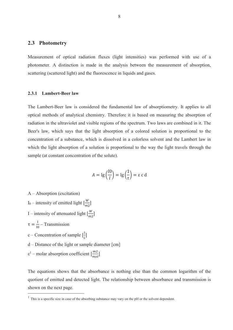
8
23 Photometry
Measurement of optical radiation fluxes (light intensities) was performed with use of a
photometer A distinction is made in the analysis between the measurement of absorption
scattering (scattered light) and the fluorescence in liquids and gases
231 Lambert-Beer law
The Lambert-Beer law is considered the fundamental law of absorptiometry It applies to all
optical methods of analytical chemistry Therefore it is based on measuring the absorption of
radiation in the ultraviolet and visible regions of the spectrum Two laws are combined in it The
Beers law which says that the light absorption of a colored solution is proportional to the
concentration of a substance which is dissolved in a colorless solvent and the Lambert law in
which the light absorption of a solution is proportional to the way the light travels through the
sample (at constant concentration of the solute)
A ndash Absorption (excitation)
I0 ndash intensity of emitted light
I ndash intensity of attenuated light
ndash Transmission
c ndash Concentration of sample
d ndash Distance of the light or sample diameter [cm]
ε1 ndash molar absorption coefficient
The equations shows that the absorbance is nothing else than the common logarithm of the
quotient of emitted and detected light The relationship between absorbance and transmission is
shown on the next page 1 This is a specific size in case of the absorbing substance may vary on the pH or the solvent dependent
9
Figure 2 Relation between transmittance and absorbance (httpteachingshuacuk 2014)
The Law states that the fraction of the light absorbed by each layer of solution is the same which
leads to a linear function instead of a logarithmic function by using the Absorbance In terms of
analysis it is easier to have linear function This is why the effect is mainly displayed as a
function of absorbance
Usually the scattering and luminescence effects in the spectroscopy analysis are neglected
Therefore in this work the term absorbance is used (when not specified otherwise) since
extinction is the sum of the effects of absorption scattering and luminescence (Mills Cvitaš
Homann Kallay amp Kuchitsu 1993)
The law applies only under certain conditions Firstly the dissolved substance must be
homogeneously distributed in the cuvette Furthermore it should be noted that the law does not
apply for open-end concentrations This means there is a limit to the concentration that is
measurable After a certain point the absorbance no longer increases in a linear fashion caused
by an over concentration of molecules in the solution In this case light rays can no longer pass
through the medium and correspondingly it is necessary to dilute the sample
10
232 Photometer
A Photometer is in a broad sense a device that is used in biology medicine physics and
chemistry for measuring the light absorption especially for the determination of concentrations
of known substances The main approach is to illuminate a sample and to measure the resulting
light intensity with a detector Different measurement methods are used The following figure
shows the principle of the basic process with one light beam using the example of absorption
measurement
The light source (L) emits a light beam through the medium to be measured in the measuring cell
(M) and the photodetector (Ph) measures the intensity of the remaining light In the amplifier
(V) the electric signal is amplified and output as a measured value
The light source can be a tungsten mercury cadmium H2 or a D2 lamp depending on the used
spectrum Tungsten lamps for example are used in the visible wavelength range and mercury and
cadmium light sources in the ultraviolet wavelength region (wwwphotometercom 2014)
Figure 3 Structure of a photometer (wwwphotometercom 2014)
11
233 Spectrophotometer
Table 2 Specifications of the used T80 spectrophotometer
Double-beam optical system Instrument Type T80 Spectral Bandwidth 2 nm (fixed slit)
Working Mode MPU ModePC Mode
Software Support MPU Software PlatformSpec UV software workstation
Wavelength Range 190 - 1100nm Wavelength Accuracy plusmn 03nm (Automatic wavelength correction) Wavelength Reproducibility 02 nm Stray Light lt 012T (220nm Nal 340nm NaNo2)
Photometric Mode Transmittance Absorbance Energy
Photometric Range -03 - 3Abs
Photometric Accuracy
plusmn 0002 Abs (0 - 05A) plusmn 0004 Abs (05 - 1A) plusmn 03 T (0 - 100 T)
Photometric Reproducibility 0002 Abs (05 - 1A) 015 T (0 ndash 100 T )
Baseline Flatness plusmn 00015 Abs (190 - 1100nm) Baseline Stability 00008 Absh (500nm0Abs 2nm Spectral
Bandwidth 2hr warm-up_ Spectral Bandwidth 2nm (fixed slit) Photometric Noise plusmn 0001 Abs (500nm 0Abs 2nmSpectral
Bandwidth)
In the case of the spectrophotometer white light is decomposed by a prism or a diffraction
grating so that only light with a specific wavelength can pass through a shutter and into the
sample solution With lenses and apertures a narrowly defined light beam is produced consisting
of parallel rays By using filters or monochromators the spectrum of the light is reduced to a
limited wavelength range
While the light passes through the sample a part of the incident light is absorbed by the
molecules in the solution causing a weakening of the light intensity which can be recognized by
the photo detector and the attenuation of light is calculated by a computer (Lehmann 1892)
12
The light attenuation is a measurement of the absorption of light and is therefore a measurement
of the concentration of the absorbing molecules in the analyzed solution In this way the
concentration of the substance can be determined using the Lambert-Beer law or a calibration
curve (Boumlcker 1979)
The final aim of the measurement is the detection of the attenuation of the light intensity by the
substance in the measuring cell The measurement result depends on the brightness of the light
source (L) and the sensitivity of the photodetector (Ph) However the properties of these
components change under the influence of fluctuations in the supply voltage temperature and
aging The single-beam therefore is not stable in the long run and must be frequently
recalibrated (wwwphotometercom 2014)
This may be justifiable for individual measurements in the laboratory but in the context of
industrial settings continuous measurement influences of the light source fluctuations have to be
eliminated This leads to the dual-beam method
Figure 4 Structure of a photometer with a dual-bean (wwwphotometercom 2014)
Here a semi-transparent mirror splits the ray into two beams a measurement beam (M) which
passes through the sample and impinges on a first photodetector and a reference beam (V) which
falls directly on a second receiver
The measured value is created by forming a ratio so that the variations in the luminosity of the
light source have no effect However a remaining error source is the change in the sensitivity of
the two photodetectors Therefore the optimum solution is to use two beams and only one
photoreceptor During the project an UVVIS Spectrophomater (model T80 from PG Insturments
Ltd) was used which works exactly in the described manner
13
Figure 5 Dual beam measuring method with only one photodetector (wwwphotometercom 2014)
Again the measured value is created by calculating the ratio of the sample and reference beams
Due to a rotating disc profile (Chopper) the two beams alternate on the same photo detector This
eliminates not only the variations in the light source but also changes of sensitivity of the
photoreceptor are eliminated (Spektrum 1999)
24 Fluorimeter
Table 3 Specifications of the used FluoroMaxR Fluorimeter
FluoroMaxR-4 with USB von HORIBA Lamp Vertically mounted CW 150 W Ozone-free xenon
arc lamp Gratings 1200 groovemm blazed at 330 nm (excitation) and
500 nm (emission) plane ruled Detectors Emission R928P photon counting PMT (185-850
nm) and reference photodiode for monitoring lamp output
Water Raman SN 60001 (RMS method) See Signal-to-noise ratio Slits Continuously variable from 0 to 30 nm Accuracy 05 nm Repeatability 01 nm Minimum step 00525 nm Integration time 0001 to 160 sec Software FluorEssence Monochromators Automatic self-calibration of all wavelength drives
and slits All reflective optics Czerny-Turner spectrometers
Spectral Correction Factors Included
14
Fluorometry is a molecule-spectroscopic analysis that utilizes the property of electronically
excited molecules to emit the absorbed excitation energy as luminescence radiation Since the
electronic excitation of the molecules take place by absorption of light fluorimetry is a
photoluminecense method It finds versatile applications in both organic and inorganic analysis
The outstanding features of this method are their high selectivity and high sensitivity (Zander
1981)
The process is characterized particularly by some features At first it is a direct photometric
method for qualitative and quantitative analysis It is highly sensitive and has a wide range of
linearity Furthermore there are small amounts of material required for the analysis Online as
well as in-situ analysis are possible Lastly there is no or little sample preparations required
which leads to a non-destructive procedure That means the sample can be returned without
problems (Zander 1981)
Fluorimetry is generally based on the detection of emitted luminescent radiation from a sample
or a photochemical mediator molecule (fluorescent marker)
Luminescence radiation arises when electrons move from a higher to a lower orbital This is
called Stokes shift Stokes fluorescence is the re-emission of longer wavelength photons (lower
frequency or energy) by a molecule that has absorbed photons of shorter wavelengths (higher
frequency or energy) It is characteristic for every substance (Schmidt 2000)
A prevention of fluorescence by other types of dissipation of the excitation energy may occur
For instance an energy transfer to other molecules without radiation (eg photosynthesis) or
internal conversion
The intensity of the fluorescence of a solution depends on the intensity of the excitation light
(Iα) the molar absorption coefficient ε of the fluorescent substance the concentration c of the
sample and the quantum yield Q
I0 ndash intensity of emitted light
Ia ndash intensity of attenuated light
15
c ndash Concentration of sample
d ndash Distance of the light or sample diameter
ε ndash molar absorption coefficient
Fluorimetry is used especially often in the field of quantitative analysis because in this case the
detection sensitivity is much higher than for pure absorption photometry The reason is the ratio
of the absorption photometry where usually slightly different signals are measured (Boumlcker
1979)
The majority of chemical compounds have a fluorescence ability Almost all aromatic
hydrocarbons are characterized by fluorescence assets Nevertheless the introduction of
substituents derogates this Particularly nitro and carboxylic acid as well SH-groups and related
substituents almost completely delate the fluorescence (Schmidt 2000)
Fluorimetry has a high detection limit of 10-12 Mol whereas in the absorption analysis only up
to 10-8 Mol can be detected At high substrate concentrations attention should be paid to the fact
that the fluorescence intensity Q is no longer a linear function of the concentration c To stay in
the linear range a maximum concentration of should not be exceeded In the following
figure the structure of a fluorimeter device is presented
Figure 6 Common structure of a fluorimeter device (Rouilly 2014)
16
Mercury or xenon lamps are often used as sources of excitation light Mercury vapor lamps emit
a line spectrum with high intensities in the lines (at 254 313 36566 405 546 577 630 nm )
via a low-intensity continuous background Xenon lamps have a continuous emission spectrum
but its intensity decreases in the UV range
Important properties of monochromators are their light intensity the spectral slit width and the
freedom of scattered light In modern appliances imaging holographic gratings are used All
optical elements such as lenses gratings mirrors and beam splitters influenced by their spectral
characteristics influence the intensity and polarization of the reflected and transmitted radiation
as a function of wavelength
Photomultiplier are used as which allow due to their high amplification (106 to 108) the
measuring of lower light intensities up to single photons Depending on the material of the
photocathode different types of photoreceptors can vary in terms of their absolute and spectral
sensitivities The gain of the photomultiplier depends on the applied voltage (Zander 1981)
25 Prototype
The instrument which was used for this project was designed to measure and analyze samples of
microalgae by using the method of a fluorimeter In line with the idea of inexpensive production
the construction is relatively basic A schematic diagram is presented in the graphic below
Figure 7 schematic diagram of the prototype sensor (left) and photo (right) (Rolim Heinen amp Huff 2014)
17
As is shown above the installation is similar to the fluorimeter (qv figure 6) The main
components are an LED light source which sends a light beam into an opaque chamber where
the sample is placed and two optical receptors which are positioned at angles of 180deg and 90deg
In contrast to the fluorimeter only one filter is used here (in the fluorimeter three mochrometers
were used) The filter works in the same manner as the monochrometer and blocks all unwanted
wavelengths so that just one specific or particular spectrum can pass through
Figure 8 Filter ldquoStrawrdquo to eliminate unwished wave length
The filter absorbs undesired wavelengths between 300 and 400 nm but has a transmission of 88
in case of the important spectrum (lt 400 nm) which is not optimal but a calculable factor
since itrsquos the same loss in any sample and series of tests
Even though lasers have excellent characteristics in case of accuracy and wavelength they are
relatively expensive In opposition to LEDs In opposition to LEDs Caused by that an LED light
source is installed together with the two optical sensors The high potency LED lamp emits a
blue light beam which fits well with the potential spectrum of absorbance of the chlorophyll and
should provide optimal requirements for the microalgae
18
26 Measurement of Biomass
The analyses of the biomass provides information about growth rate and as a consequence
thereof biological activity Therefore a vacuum pressure pump was used together with paper
filters with a diameter of 205 μm and a pore size of 14 μm
A sample of 50 ml was taken from the batches and filtered through the paper (weighted before)
while the vacuum pump supported the passaging of the liquid Afterwards the nearly-dry paper
was stored in an oven at 60 degC for approximately 24 hours The mass difference gives some
indication of the amount of biomass in the 50 ml solution
27 Measurement of Chlorophyll
An issue in chlorophyll measurement is extracting the pigments from the cells Therefore a
sample of 10 ml is filtered (same procedure as for biomass) The extract is stored afterwards in a
90 acetone solution at 4 degC for approximately 24 hours Acetone is a moderate polar solvent
which is after methanol the best solution for chlorophyll pigments because it consists of polar
areas as well as a lipophilic phytel rest (see figure 9) (Lourenccedilo 2006)
Figure 9 Chemical structure of chlorophyll (Willows 2013)
19
Due to the reference (Lourenccedilo 2006) the solution should be centrifuged for around 10 minutes
and 3000 rpm This strategy is used because usually the filter is cut in pieces before stored in the
tube to guarantee a better detachment of the chlorophyll The pre-tests have shown that the
results are more accurate when the filter isnrsquot cut but rolled up and put into the tube (filtrate
towards the tubes inside) If than filled carefully up with acetone (washing out of the extract
must be avoided during infusion) the extraction of chlorophyll will be optimal without the
problem of filter rests and other cell bodies
In a further step the chlorophyllacetone solution is measured in a spectrophotometer by 630 nm
647 nm and 663 - 665 nm The amount of chlorophyll is calculated by the following statistic
equations from Lourenccedilo (2006)
D663-665 D647 D630 ndash absorbance at the wavelength Dx after correction by the cell-to-cell blank and subtraction of the cell-to-cell blank corrected absorbance at 750nm
l - Cell (cuvette) length [cm] = 1
v - Volume of acetone [ml] = 10
V - Volume of filtered water [l] = 10
Accordingly the term That simplifies the equations
20
3 Results and discussion
During the project the algae suspension was scanned over a time interval of 10 days plus one
day incubation During this time the batches were subjected to various light conditions (Batch A
= 4000 Lux Batch B = 5500 Lux Batch C = 7000 Lux Batch D = 8500 Lux Batch E = 10000
Lux) This was performed to analyze the effect of different light intensity on algae and
accumulation of chlorophyll To obtain useful results it is essential to eliminate as much
unwished problems as possible According to this the growing of the algae was analyzed at first
because any discrepancies of the algae growth would lead to consequential errors in case of
chlorophyll tests
31 Algae growth The growth of Scanedesmus Sp was measured via spectrophotometer and biomass dry weight
Optical density of biomass was determined at 750 nm One ml of the sample batch was taken and
measured in a spectrum between 400 nm and 750 nm
Usually the growth of an algae culture follows certain steps It starts with the lag phase (1)
followed by an exponential phase (2) The culture growth will reach a point of overpopulation in
which one or more essential resources are limited Growth and death rate are either in
equilibrium or the cells already stopped the proliferation This is called the stationary phase (4)
At the end the living conditions are so bad that the cell population starts to decrease rapidly
(usually caused by a deficiency of important nutrients) The last phase is called death phase (5)
Figure 10 Sketch of algae growth dynamics
21
The before explained growth dynamic differs to the culture development during the test Figure 7
(below) presents all graphs (of absorbance [400hellip750 nm]) of the five batches in a time interval
of ten days So in total 50 single graphs summarized in that 3D - graphic It gives an interesting
overview of the total experiment
Figure 11 Progress of all 5 batches in a time interval of 11 days
In the figure a formation can be seen that looks like one side of a steep ridge that starts relatively
flat in the beginning and becomes steeper in the posterior tier Rifts in the formation are caused
by some problems associated with the spectrophotometer at certain wavelengths Following the
observation that the results are the same regardless of the kind of sample analyzed the
assumption that the spectrophotometer doesnrsquot work at these wave length may be accepted
Furthermore a pattern of wave formations is recognizable Every wave formation has a
maximum at around 400 nm and 480 nm and between 650 nm and 670 nm The first ldquowaverdquo is
the result of the batch analyses from the first day the second from the second day and so on
The wavelike formation is caused by the differential growth of the algae under different light
22
conditions The most exposed batch (E) already has a higher algae concentration on dayx as
compared to the lowest exposed batch (A) one day after
Figure 12 By comparison absorbance between 400 nm and 750 nm of five batches at day 6 and 72
The first figure curvebatch E has the highest absorbance starting between 06 and 065 at 400
nm and ending up at the second maximum at around 059 In comparison batchcurve A from
one day after also starts between 06 and 065 but falls under the values of Batch E at the second
maximum which occurs at around 056 This is responsible for the wave effect between the
days Only at the last day does Batch A exceed the high peaks of Batch E from the previous day
This is caused by the beginning of the exponential phase Unfortunately the cultures did not pass
through all four phases as expected The exponential phase started between day 7 and 9
depending on the Batch
2 The days are chosen randomly to proof the above delineated statement The same course of curves could be confirmed for every day Just the intensity of absorbance varies
23
We can see the effect of light between the different figures The culture of Batch E already began
exponential growth at day 7 while the lag phase in Batch A persisted until the 8th9th day
Figure 13 Progress of culture growth comparing Batch E (left) and A (right) during the 10 days in comparison to the Absorbance
The following statements can be made to summarize the observed algae growth Since the
different colonies in the Batches react to the light intensity as expected the assertion can be
made that the Biomass (mB) of
When comparing the results of the optical density with the gravimetric measurements some
issues have to be mentioned The dry weight measurement was only performed after day four
because the amount of biomass measured before day five was considered too small to be reliably
assessed Even after the fifth day some unexpected changes in the curve shape were visible
Nonetheless the main shape of the curve approximates an exponential slope after day eight
which is consistent with the measurement of the optical density
24
Figure 14 Dry weight (mgl) of Scenedesmus Sp for 10 days grown under different light conditions
In addition the amount of biomass increases daily in every Batch according to the results of the
optical density
This is not so in the case of the dry weight measurement where no decipherable pattern can be
determined for the first half of the test period Some problems occurred during the laboratory
processing including the malfunctioning of an oven during day 6 and a restoration of the
samples during day seven Additionally as a consequence of the high error-proneness of the
earlier dry weight analysis due to the use of relatively small volumes findings from the dry
weight analyses should be considered with caution
Beyond these issues it has to be mentioned that the colonies didnrsquot reach the stationary phase
and thus also failed reach the death phase These two statuses of the growth dynamic could
have been interesting for the comparison of the algaechlorophyll ratio while exposed to different
light intensities
25
The results of biomass and spectrophotometer analyses confirm the findings of the designed
prototype in the way that the order of the batches in proportion to dissolved substances (
biomass) is the same as the order of the Batches themselves (BA lt BB lt BC lt BD lt BE dayx)
Figure 15 Algae development measured by prototype during the days 7 - 11 plotted as a function of voltage
The figure above shows the general light intensity that passes through the sample filled with
water (~ 245 V) The larger the amount of dissolved material in the sample the less light will
pass through it and consequently the lower the measured voltage will be With a general
tendency toward a lower voltage a larger amount of biomass can be ascertained but it has to be
mentioned that no statements about the type of curve shape can be made Unfortunately more
test results would have been necessary to make further statements
0
05
1
15
2
25
3
7 8 9 10 11
Outp
ut vo
ltage
at 1
80deg(
V)
Days
A
B
C
D
E
Water
26
32 Chlorophyll formation
After the chlorophyll-acetone mix is stored for 24 hours it is analyzed with a spectrophotometer
For the calculation of chlorophyll content according to Jeffrey amp Humphrey (1975) only some
wavelengths are important Nevertheless the chlorophyll was treated in the same way as the
algae and measurements were made in the range of 400 nm to 750 nm in order to determine
possible similarities
Figure 16 Chlorophyll (mgl) of Scenedesmus sp for 10 days grown under different illumination conditions
The concentration of total chlorophyll increases during the test The results show a steady growth
if expressed as the exponential regression curve (dotted lines) for Batches D and E (R = 09) A
better correlation is shown for a linear regression for Batches A and B (R = 09 instead of 076)
Batch C doesnrsquot show a strong correlation under either a linear (R = 072) or an exponential
growth (R = 076) assumption Many factors affect the results of the Chlorophyll measurement
Firstly the analyses are susceptible to mistakes made during the processing When removing 10
ml from the batches with a concentration of barely 1 mgL and using those samples in a cuvette
of 3 mL the amount of Chlorophyll is typically in a range of 0 ndash 10 μgmL Working with such
small quantities can lead to inaccuracies during processing in addition to errors made on behalf
of the measuring engine itself
Rsup2 = 07602
Rsup2 = 07602
Rsup2 = 09004
Rsup2 = 09037
Rsup2 = 07594
0
05
1
15
2
25
0 1 2 3 4 5 6 7 8 9 10 11
Chlo
roph
yll a
+b (m
gl)
Day
C
D
E
B
A
Expon (C)
Expon (C)
Expon (C)
Expon (D)
Expon (D)
Expon (E)
Linear (B)
Expon (A)
Linear (A)
27
Nevertheless we can make the assumption that the tendency (daily increase) makes sense The
results of the pilot engine show slightly decreasing curves At day 8 there is an obvious mistake
to declare This is not visible with regard to algae measurement at day 93 This leads to the
assumption of a mistake made during the preparing procedure with acetone Since the
abnormality can be found in all batches a mistake during the withdrawal can be ruled out
Figure 17 Chlorophyll development during the days 7 - 11 plotted as a function of voltage
A further problem is that the curves are not clearly separable They cross each other without
showing a decipherable trend with regard to which batch has the highest or the lowest
translucency (which would be proportional to the voltage) As a consequence these results
cannot provide information about the effect of different light irradiation and it is questionable
whether they can be used to make an assumption about chlorophyll accumulation
3 The spectrophotometer analyzes of chlorophyll is one day after due to the 24 hours storing of the samples
0
05
1
15
2
25
3
7 8 9 10 11
Outp
ut vo
ltage
at 1
80deg(
V)
Days
E
B
C
D
A
Water
28
33 Correlation of Algae and Chlorophyll growth The main rationale for using different light irradiation for the Batches was to determine the
relationship between algae growth and the Chlorophyll enhancement Hence interest lay beyond
simply examining the thesis that the concentration of Chlorophyll is directly linked to the algae
growth Furthermore there was interest in exploring whether a specific relationship existed
between the algae growth rate the exposure to light and the amount of chlorophyll produced
Figure 18 Collocation of AlgaeChlorophyll absorbance (by 665 nm) by a spectrophotometer for 11 days
Unfortunately an incomplete test phase (no algae growth until the stationary phase) was
responsible for a lack of results that could be used for further analysis Nevertheless the ratio of
Chlorophyll-to-Algae growth shows a decent progression (see also Table 4) There is no
evidence for a similar progression if the tests proceed for one or two weeks In theory the
chlorophyll concentration should increase more rapidly in the exponential phase (until now the
progress is best described as a linear growth) Furthermore the concentration of algae as well as
of chlorophyll from batch E should reach its maximum first followed by batch D C B A (in
this order) and continue at a stationary rate
BAA
lgae
BAC
hlBB
Alg
aeBB
Chl
BCA
lgae
BCC
hl
BDA
lgae
BDC
hl
BEA
lgae
BEC
hl
002040608
112141618
12
34
56
78
9 1011
BatchSubstrate
Abso
rban
ce
Days
BAAlgae
BAChl
BBAlgae
BBChl
BCAlgae
BCChl
BDAlgae
BDChl
BEAlgae
BEChl
29
Due to the issues described in the earlier chapters the results from analyses on biomass are less
convincing than those arising from the analyses of the spectrophotometer In addition and
contrary to the absorbance measurement the values of dry weight and calculated chlorophyll
correlate weakly in cases of batches with higher light saturation This may be due to inaccuracies
from the dry weight results or another reason could be the earlier start of a kind of exponential
growth for the chlorophyll while the results for the biomass donrsquot show an exponential increase
until the 7th day
Table 4 Overview of the results of biomass prototype and spectrophotometer analyzes
Substrate Biomass (mgl) ndash Dry weight and Chl Optical density (V) -
Prototype Absorbance - Spectrophotometer
Min Max R Min Max R Min Max R BAAlgae 146 327
092 185 061
- 013 156
094 BAChl 001 164 212 170 001 017 BBAlgae 154 444
085 124 049
- 013 169
089 BBChl 004 172 206 175 001 026 BCAlgae 170 478
078 097 042
- 012 170
082 BCChl 002 188 194 181 001 023 BDAlgae 162 504
068 104 044
- 011 172
094 BDChl 002 124 196 171 001 026 BEAlgae 160 515
066 130 035
- 009 175
097 BEChl 002 114 215 195 001 031 The less exciting results are unfortunately given by the Prototype Here no significant correlation
can be mentioned at all In contrast to the spectrophotometer these values are provided by the
direct transmission Therefore the highest solution has the lowest value because more light is
absorbed by the dissolved material which is in this case biomass (or pure chlorophyll) This
result is surprisingly disappointing because the tests performed beforehand with fluorescence
(realized by Leonardo M Rolim) show a straight dependency of proportional relationship
between percental solution and transmission (see Figure 19 below)
Fluorescein is a fluorescent dye from the group of the xanthene It was used for the previous tests
because itrsquos a non-biological and well known substance with which all unwished side effects of a
living system can be avoided during tests
30
Figure 19 Measuring points of concentration given in optical density from fluorescence (Rolim Heinen amp Huff 2014)
The graph shows the transmission by 180 degC as accomplished with the algae and chlorophyll
during this work The curve suggests a negative exponential trend This was also expected for the
new series of tests While a clear difference can be recorded in the case of fluorescein the values
of chlorophyll almost didnrsquot change This could be an effect of the high fluorescent impact of
fluorescence Due to the growth rate of chlorophyll (see Table 4 Chl Min and Max) which goes
from 001 gmL up to almost 18 gmL (180 times more) compared with the fluorescence which
goes from 001 gmL up to 03 gmL (30 times more) this is questionable since the concentration
difference is 5 times higher for pure chlorophyll a fluorescent pigment as well but the effect is
very little Nevertheless it could be an indication as to why results from the test were not as
expected
The analyses by the fluorimeter provides further interesting results The figure below presents
the results of chlorophyll for the 11th day The x-axis shows the input of the wave length
produced by the laser The excitation is visible on the y-axis while curves on the graph present
one specific wave length each between 400 and 800 nm (with an interval of 5 ie a new
measurement was performed for every 5 nm) In order to simplify the graphical presentation the
legend was omitted
31
Figure 20 Display of emission and excitation measured by the fluorimeter of day 11 for chlorophyll
The figure provides an important insight into the behavior of chlorophyll fluorescent The
formation on the bluish part of the light spectrum (270 ndash 430 nm) and the second cluster of peaks
between 650 and 675 nm are quite revealing The table below explains the most important
curves
Table 5 Legend of figure 16
Color wave length (nm) red 675 blue 670 gray 680
light green 665 orange 685
light blue 660 dark blue 690 dark green 695
These eight curves are explicitly mentioned because they have the highest response in the tested
emission spectrum Due to usually low concentrations of samples eg chlorophyll in μgml a
high response is vital The results of the other test days are equal They simply vary in the height
of excitation as a result of a higher concentration
0
200000
400000
600000
800000
1000000
1200000
1400000
1600000
300 325 350 375 400 425 450 475 500 525 550 575 600 625 650 675 700 725 750
Exita
tion
ampe
rage
at 9
0deg(m
A)
Emission wave lenght (nm)
32
Figure 21 Display of emission and excitation measured by the fluorimeter between the days 0 and 11 for chlorophyll (BA)
The daily difference of the excitation is presented above The course of the curves is equal and
just differs as mentioned before in the amount of ampere measured by the receptor The same
shape would be plotted by the other batches The only difference again would be the level of
excitation
The progression of the chlorophyll curves during the tests shows a permanent increase beginning
at day three An exponential correlation can be verified for the plotted curves Thus the results
from the fluorimeter are as expected before Still the problem as mentioned before of the
incomplete growth of the algae was responsible for a lack of further information which could
have been interesting
0
200000
400000
600000
800000
1000000
1200000
350 375 400 425 450 475 500 525 550 575 600 625 650 675 700 725 750
Excit
atio
n am
pera
ge a
t 90
deg(m
A)
Emission wave lenght (nm)
0
1
2
3
4
5
6
7
8
9
10
11
33
Figure 22 Trend of the chlorophyll excitation peaks during 11 days measured by the fluorimeter
In the following section the results from the algae analyses are explained One problem has to be
mentioned beforehand
The graph below shows the outcome from the last day Highly overlapping curves are visible
This is not caused by fluorescence but by the reflection of each wave length itself due to a high
solution The analyses made by the fluorimeter requires at least 30 minutes That it enough time
for the dissolved particle to settle down The x-axis can accordingly be viewed as a timeline
scale As more time passes by the reflection impact reduces
Rsup2 = 08453
0
200000
400000
600000
800000
1000000
1200000
1400000
1600000
1800000
2000000
0 2 4 6 8 10 12
Excit
atio
n am
pera
ge a
t 90
deg(m
A)
Days
660
665
430
405
375
Log (375)
34
Figure 23 Fluorimeter results of algae (BA day11)4
When the y-axis is limited to 100000 mA some other formations are visible Interestingly they
have the same shape as the curves of the chlorophyll which leads to the assumption that those
overlapped curves are indeed the fluorescent impact of the chlorophyll pigments
4 Every curve presents one wave length of the emission spectrum in an interval of five The legend is once more excluded due to a better overview
0
1000000
2000000
3000000
4000000
5000000
6000000
7000000
8000000
300 325 350 375 400 425 450 475 500 525 550 575 600 625 650 675 700 725 750
Excit
atio
n am
pera
ge a
t 90deg
(mA)
Emission wave lenght (nm)
35
Figure 24 Fluorimeter results of algae (BA day11) with limited y-axes up to 100000 mA5
On closer examination it can be interpreted that the higher curves (blue orange green dark
blue redhellip) are the same wavelengths as seen in the Table 5 Legend of figure 16rdquo The highest
response again is at 675 nm Measureing by a different wave length than 675 nm will cause
lower excitation The same happens in case of chlorophyll
The excitation is low in comparison with the results of the pure chlorophyll because the
chlorophyll is not separated from the cells which hinders the light from reaching the pigments
in addition to leaving the sample and stimulating the receptor
The comparison with the other batches and the analyses of the different days provides the same
results as for the chlorophyll That means the Excitation of BA(dx) lt BB(dx) lt BC(dx) lt BD(dx)
lt BE(dx) and the Excitation of BA(dx) lt BA(dx+1) BB(dx) lt BB(dx+1) BC(dx) lt BC(dx+1)
BD(dx) lt BD(dx+1) BE(dx) lt BE(dx+1)
5 The legend is once more excluded due to a better overview
0
10000
20000
30000
40000
50000
60000
70000
80000
90000
100000
300 325 350 375 400 425 450 475 500 525 550 575 600 625 650 675 700 725 750
Excit
atio
n am
pera
ge a
t 90
deg(m
A)
Emission wave lenght (nm)
36
4 Conclusiones
According to the results from the fluorimeter the algae growth and chlorophyll enhancement
appear to be as expected This leads to the question as to why the previous tests donrsquot have
similar outcomes The answer to this question and the reason why fluorimeters are used for low
quantities is the same They have a very high accuracy and are thus extremely efficient even
for low quantities Nevertheless they are extremely expensive and the main task of this project
was to determine whether it was possible to measure chlorophyll (pure or even intracellular) with
the prototype or if not to work out further steps for the development of the engine
The first step apart from the biological section is to make the engine more stable During the
project problems often occurred with regard to replication of results because small changes in the
electrical connection contributed to different outcomes while using the same sample This made
the testing more complicated and made unnecessary repetitions of measurement indispensable A
shell for the entire construction in which the electronic is fixed should solve this problem An
extension cable which leads to the measuring box together with a smaller diameter of the cell
itself would also be useful The laser and the two receptors should be installed separately from
the cell and waterproofed (plastic and glue should be sufficient) As a result the cell could be
introduced into a sample to measure which not only simplifies the procedure but it is also closer
to any practical application
The next action is the acquisition of the correct optical filter The results of the fluorimeter
suggest an optimal emission at 430 plusmn 10 nm while the excitation should be measured at 675 plusmn 10
nm The closer the measurement is to these wavelengths the higher the values of the results
Furthermore it was explained how other wave lengths overlap the fluorescence effect This can
be avoided by use of at least two filters one which filters the light of the laser and blocks out
every wavelength except for those in the range of eg 420 ndash 440 nm and a second filter which
allows for only the spectrum from 665 to 685 nm to pass
Nevertheless an upgrade of either the receptor or laser but probably both will be inevitable As
mentioned in the previous chapter the outcome of the 90deg measurement for algae and
chlorophyll is almost zero In actuality it has the same value as if measured with water which
means that the receptor is not able to recognize any approaching light On the other hand it may
37
be that the laser is too weak so that not enough light is injected In any case adjustment for the
right filter range should be the first step
When the filter and laserreceptor problems are solved a new test with fluorescence would make
sense At this stage it is important not only that the results are good for one series of tests but
also that they are repeatable Daily calibration of the engine is not only effortful and time-
consuming but it can also lead to variable results After good and stable results are achieved
with fluoresce a new test series with algae can be started Therefore it would be useful to create
a serial dilution of an algae culture which is already in the stationary phase and highly
concentrated If the results are suitable it can be continued with a serial dilution of those algae
Even if the results from the 90deg measurement are not satisfying a further test with pure
chlorophyll could be accomplished on condition that the results from the 180deg measurement are
decent
Only after all the described experiments have sufficient results should a new long-term test series
be started For this purpose no more than three batches should be installed with an intensity of
illumination between 3000 and 10000 lux The test duration should be approximately 30 days to
ensure that the culture passes through all growing and dying phases Tests performed with the
spectrophotometer can indicate a change of the growing conditions so that further and more
elaborated tests with the fluorimeter and biomass can be performed The measurement of
biomass should be sufficient if performed every three days (a daily testing during the exponential
phase would perhaps be useful) By using the fluorimeter care has to be taken so that the dilution
of the sample is large enough otherwise overlapping effects occur The analyses with the sensor
should be performed daily in order to get a consistent overview of the chlorophyllalgae ratio as
well as to gauge the accuracy of the sensor
38
5 Bibliography Boumlcker J (1979) Spektroskopie Instrumentelle Analytik mit Atom- und Molekuumllspektroskopie
(1 Edition Ausg) Wuumlrzburg Vogel Verlag und Druck GmbH amp Co
Hegewald P (2006) Scenedesmusndashlike algae of Ukraine Tsarenko E amp B Braband
Lehmann E W (1892) Uumlber ein Photometer Erlangen
Lourenccedilo S (2006) Cultivo de Microalgas Marinhas Princiacutepios e Aplicaccedilotildees
Luumlrling M (1999) The Smell of Water Grazer-Induced Colony Formation in Scenedesmus
Wageningen Pulz und Gross
Mills I Cvitaš T Homann K Kallay N amp Kuchitsu K (1993) Quantities Units and
Symbols in Physical Chemistry (Green Book)
Rolim L M Heinen A L amp Huff D D (2014) Desenvolvimento de sensor oacuteptico portaacutetil
para mediccedilatildeoes online de concentraccedilatildeo no cultivo de microalgas Porto Alegre
Rouilly V (2014) Schmidt W (2000) Optische Spektroskopie (Bd 2 Edition) Weinheim
WILEY-VCH Verlag GmbH
Unknown (1999) Photometer Spektrum Akademischer Verlag
Willows R D (2013) Structure of chlorophyll Organic Letters
Zander M (1981) Fluorimetrie Berlin-Heidelberg-New York Springer-Verlag
Internet sources Openwetwareorg
photometercom
teachingshuacuk
wikipediaorg
39
6 List of figures Figure 1 Pilot batch deployment 7
Figure 2 Relation between transmittance and absorbance 9
Figure 3 Structure of a photometer 10
Figure 4 Structure of a photometer with a dual-bean 12
Figure 5 Dual beam measuring method with only one photodetector 13
Figure 6 Common structure of a fluorimeter device 15
Figure 7 schematic diagram of the prototype sensor (left) and photo (right) 16
Figure 8 Filter ldquoStrawrdquo to eliminate unwished wave length 17
Figure 9 Chemical structure of chlorophyll 18
Figure 10 Sketch of algae growth dynamics 20
Figure 11 Progress of all 5 batches in a time interval of 11 days 21
Figure 13 By comparison absorbance between 400 nm and 750 nm of five batches at day 6 and 7
22
Figure 14 Progress of culture growth comparing Batch E (left) and A (right) during the 10 days
in comparison to the Absorbance 23
Figure 15 Dry weight (mgl) of Scenedesmus Sp for 10 days grown under different light
conditions 24
Figure 16 Algae development measured by prototype during the days 7 - 11 plotted as a function
of voltage 25
Figure 17 Chlorophyll (mgl) of Scenedesmus sp for 10 days grown under different illumination
conditions 26
Figure 18 Chlorophyll development during the days 7 - 11 plotted as a function of voltage 27
Figure 19 Collocation of AlgaeChlorophyll absorbance (by 665 nm) by a spectrophotometer for
11 days 28
Figure 20 Measuring points of concentration given in optical density from fluorescence 30
Figure 21 Display of emission and excitation measured by the fluorimeter of day 11 for
chlorophyll 31
Figure 22 Display of emission and excitation measured by the fluorimeter between the days 0
and 11 for chlorophyll (BA) 32
Figure 23 Trend of the chlorophyll excitation peaks during 11 days measured by the fluorimeter
33
Figure 24 Fluorimeter results of algae (BA day11) 34
Figure 25 Fluorimeter results of algae (BA day11) with limited y-axes up to 100000 mA 35
40
7 List of tables Table 1 Composition of algae supplementary medium 6
Table 2 Specifications of the used T80 spectrophotometer 11
Table 3 Specifications of the used FluoroMaxR Fluorimeter 13
Table 4 Overview of the results of biomass prototype and spectrophotometer analyzes 29
Table 5 Legend of figure 16 31
41
Declaration of Authorship I hereby certify that this work has been composed by me and is based on my own work
unless stated otherwise No other person`s work has been used without due
acknowledgement in this report All references and verbatim extracts have been quoted
and all sources of information including graphs and data sets have been specifically
acknowledged
______________________ ________________________ Ort Datum Signature
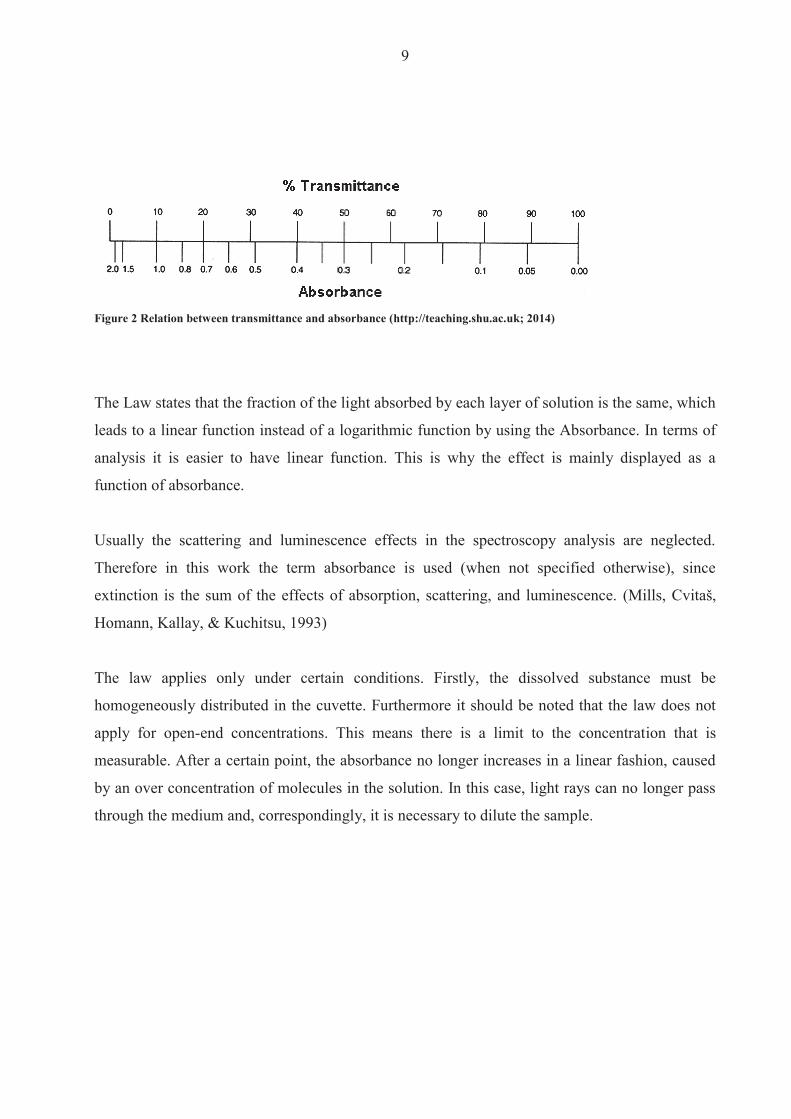
9
Figure 2 Relation between transmittance and absorbance (httpteachingshuacuk 2014)
The Law states that the fraction of the light absorbed by each layer of solution is the same which
leads to a linear function instead of a logarithmic function by using the Absorbance In terms of
analysis it is easier to have linear function This is why the effect is mainly displayed as a
function of absorbance
Usually the scattering and luminescence effects in the spectroscopy analysis are neglected
Therefore in this work the term absorbance is used (when not specified otherwise) since
extinction is the sum of the effects of absorption scattering and luminescence (Mills Cvitaš
Homann Kallay amp Kuchitsu 1993)
The law applies only under certain conditions Firstly the dissolved substance must be
homogeneously distributed in the cuvette Furthermore it should be noted that the law does not
apply for open-end concentrations This means there is a limit to the concentration that is
measurable After a certain point the absorbance no longer increases in a linear fashion caused
by an over concentration of molecules in the solution In this case light rays can no longer pass
through the medium and correspondingly it is necessary to dilute the sample
10
232 Photometer
A Photometer is in a broad sense a device that is used in biology medicine physics and
chemistry for measuring the light absorption especially for the determination of concentrations
of known substances The main approach is to illuminate a sample and to measure the resulting
light intensity with a detector Different measurement methods are used The following figure
shows the principle of the basic process with one light beam using the example of absorption
measurement
The light source (L) emits a light beam through the medium to be measured in the measuring cell
(M) and the photodetector (Ph) measures the intensity of the remaining light In the amplifier
(V) the electric signal is amplified and output as a measured value
The light source can be a tungsten mercury cadmium H2 or a D2 lamp depending on the used
spectrum Tungsten lamps for example are used in the visible wavelength range and mercury and
cadmium light sources in the ultraviolet wavelength region (wwwphotometercom 2014)
Figure 3 Structure of a photometer (wwwphotometercom 2014)
11
233 Spectrophotometer
Table 2 Specifications of the used T80 spectrophotometer
Double-beam optical system Instrument Type T80 Spectral Bandwidth 2 nm (fixed slit)
Working Mode MPU ModePC Mode
Software Support MPU Software PlatformSpec UV software workstation
Wavelength Range 190 - 1100nm Wavelength Accuracy plusmn 03nm (Automatic wavelength correction) Wavelength Reproducibility 02 nm Stray Light lt 012T (220nm Nal 340nm NaNo2)
Photometric Mode Transmittance Absorbance Energy
Photometric Range -03 - 3Abs
Photometric Accuracy
plusmn 0002 Abs (0 - 05A) plusmn 0004 Abs (05 - 1A) plusmn 03 T (0 - 100 T)
Photometric Reproducibility 0002 Abs (05 - 1A) 015 T (0 ndash 100 T )
Baseline Flatness plusmn 00015 Abs (190 - 1100nm) Baseline Stability 00008 Absh (500nm0Abs 2nm Spectral
Bandwidth 2hr warm-up_ Spectral Bandwidth 2nm (fixed slit) Photometric Noise plusmn 0001 Abs (500nm 0Abs 2nmSpectral
Bandwidth)
In the case of the spectrophotometer white light is decomposed by a prism or a diffraction
grating so that only light with a specific wavelength can pass through a shutter and into the
sample solution With lenses and apertures a narrowly defined light beam is produced consisting
of parallel rays By using filters or monochromators the spectrum of the light is reduced to a
limited wavelength range
While the light passes through the sample a part of the incident light is absorbed by the
molecules in the solution causing a weakening of the light intensity which can be recognized by
the photo detector and the attenuation of light is calculated by a computer (Lehmann 1892)
12
The light attenuation is a measurement of the absorption of light and is therefore a measurement
of the concentration of the absorbing molecules in the analyzed solution In this way the
concentration of the substance can be determined using the Lambert-Beer law or a calibration
curve (Boumlcker 1979)
The final aim of the measurement is the detection of the attenuation of the light intensity by the
substance in the measuring cell The measurement result depends on the brightness of the light
source (L) and the sensitivity of the photodetector (Ph) However the properties of these
components change under the influence of fluctuations in the supply voltage temperature and
aging The single-beam therefore is not stable in the long run and must be frequently
recalibrated (wwwphotometercom 2014)
This may be justifiable for individual measurements in the laboratory but in the context of
industrial settings continuous measurement influences of the light source fluctuations have to be
eliminated This leads to the dual-beam method
Figure 4 Structure of a photometer with a dual-bean (wwwphotometercom 2014)
Here a semi-transparent mirror splits the ray into two beams a measurement beam (M) which
passes through the sample and impinges on a first photodetector and a reference beam (V) which
falls directly on a second receiver
The measured value is created by forming a ratio so that the variations in the luminosity of the
light source have no effect However a remaining error source is the change in the sensitivity of
the two photodetectors Therefore the optimum solution is to use two beams and only one
photoreceptor During the project an UVVIS Spectrophomater (model T80 from PG Insturments
Ltd) was used which works exactly in the described manner
13
Figure 5 Dual beam measuring method with only one photodetector (wwwphotometercom 2014)
Again the measured value is created by calculating the ratio of the sample and reference beams
Due to a rotating disc profile (Chopper) the two beams alternate on the same photo detector This
eliminates not only the variations in the light source but also changes of sensitivity of the
photoreceptor are eliminated (Spektrum 1999)
24 Fluorimeter
Table 3 Specifications of the used FluoroMaxR Fluorimeter
FluoroMaxR-4 with USB von HORIBA Lamp Vertically mounted CW 150 W Ozone-free xenon
arc lamp Gratings 1200 groovemm blazed at 330 nm (excitation) and
500 nm (emission) plane ruled Detectors Emission R928P photon counting PMT (185-850
nm) and reference photodiode for monitoring lamp output
Water Raman SN 60001 (RMS method) See Signal-to-noise ratio Slits Continuously variable from 0 to 30 nm Accuracy 05 nm Repeatability 01 nm Minimum step 00525 nm Integration time 0001 to 160 sec Software FluorEssence Monochromators Automatic self-calibration of all wavelength drives
and slits All reflective optics Czerny-Turner spectrometers
Spectral Correction Factors Included
14
Fluorometry is a molecule-spectroscopic analysis that utilizes the property of electronically
excited molecules to emit the absorbed excitation energy as luminescence radiation Since the
electronic excitation of the molecules take place by absorption of light fluorimetry is a
photoluminecense method It finds versatile applications in both organic and inorganic analysis
The outstanding features of this method are their high selectivity and high sensitivity (Zander
1981)
The process is characterized particularly by some features At first it is a direct photometric
method for qualitative and quantitative analysis It is highly sensitive and has a wide range of
linearity Furthermore there are small amounts of material required for the analysis Online as
well as in-situ analysis are possible Lastly there is no or little sample preparations required
which leads to a non-destructive procedure That means the sample can be returned without
problems (Zander 1981)
Fluorimetry is generally based on the detection of emitted luminescent radiation from a sample
or a photochemical mediator molecule (fluorescent marker)
Luminescence radiation arises when electrons move from a higher to a lower orbital This is
called Stokes shift Stokes fluorescence is the re-emission of longer wavelength photons (lower
frequency or energy) by a molecule that has absorbed photons of shorter wavelengths (higher
frequency or energy) It is characteristic for every substance (Schmidt 2000)
A prevention of fluorescence by other types of dissipation of the excitation energy may occur
For instance an energy transfer to other molecules without radiation (eg photosynthesis) or
internal conversion
The intensity of the fluorescence of a solution depends on the intensity of the excitation light
(Iα) the molar absorption coefficient ε of the fluorescent substance the concentration c of the
sample and the quantum yield Q
I0 ndash intensity of emitted light
Ia ndash intensity of attenuated light
15
c ndash Concentration of sample
d ndash Distance of the light or sample diameter
ε ndash molar absorption coefficient
Fluorimetry is used especially often in the field of quantitative analysis because in this case the
detection sensitivity is much higher than for pure absorption photometry The reason is the ratio
of the absorption photometry where usually slightly different signals are measured (Boumlcker
1979)
The majority of chemical compounds have a fluorescence ability Almost all aromatic
hydrocarbons are characterized by fluorescence assets Nevertheless the introduction of
substituents derogates this Particularly nitro and carboxylic acid as well SH-groups and related
substituents almost completely delate the fluorescence (Schmidt 2000)
Fluorimetry has a high detection limit of 10-12 Mol whereas in the absorption analysis only up
to 10-8 Mol can be detected At high substrate concentrations attention should be paid to the fact
that the fluorescence intensity Q is no longer a linear function of the concentration c To stay in
the linear range a maximum concentration of should not be exceeded In the following
figure the structure of a fluorimeter device is presented
Figure 6 Common structure of a fluorimeter device (Rouilly 2014)
16
Mercury or xenon lamps are often used as sources of excitation light Mercury vapor lamps emit
a line spectrum with high intensities in the lines (at 254 313 36566 405 546 577 630 nm )
via a low-intensity continuous background Xenon lamps have a continuous emission spectrum
but its intensity decreases in the UV range
Important properties of monochromators are their light intensity the spectral slit width and the
freedom of scattered light In modern appliances imaging holographic gratings are used All
optical elements such as lenses gratings mirrors and beam splitters influenced by their spectral
characteristics influence the intensity and polarization of the reflected and transmitted radiation
as a function of wavelength
Photomultiplier are used as which allow due to their high amplification (106 to 108) the
measuring of lower light intensities up to single photons Depending on the material of the
photocathode different types of photoreceptors can vary in terms of their absolute and spectral
sensitivities The gain of the photomultiplier depends on the applied voltage (Zander 1981)
25 Prototype
The instrument which was used for this project was designed to measure and analyze samples of
microalgae by using the method of a fluorimeter In line with the idea of inexpensive production
the construction is relatively basic A schematic diagram is presented in the graphic below
Figure 7 schematic diagram of the prototype sensor (left) and photo (right) (Rolim Heinen amp Huff 2014)
17
As is shown above the installation is similar to the fluorimeter (qv figure 6) The main
components are an LED light source which sends a light beam into an opaque chamber where
the sample is placed and two optical receptors which are positioned at angles of 180deg and 90deg
In contrast to the fluorimeter only one filter is used here (in the fluorimeter three mochrometers
were used) The filter works in the same manner as the monochrometer and blocks all unwanted
wavelengths so that just one specific or particular spectrum can pass through
Figure 8 Filter ldquoStrawrdquo to eliminate unwished wave length
The filter absorbs undesired wavelengths between 300 and 400 nm but has a transmission of 88
in case of the important spectrum (lt 400 nm) which is not optimal but a calculable factor
since itrsquos the same loss in any sample and series of tests
Even though lasers have excellent characteristics in case of accuracy and wavelength they are
relatively expensive In opposition to LEDs In opposition to LEDs Caused by that an LED light
source is installed together with the two optical sensors The high potency LED lamp emits a
blue light beam which fits well with the potential spectrum of absorbance of the chlorophyll and
should provide optimal requirements for the microalgae
18
26 Measurement of Biomass
The analyses of the biomass provides information about growth rate and as a consequence
thereof biological activity Therefore a vacuum pressure pump was used together with paper
filters with a diameter of 205 μm and a pore size of 14 μm
A sample of 50 ml was taken from the batches and filtered through the paper (weighted before)
while the vacuum pump supported the passaging of the liquid Afterwards the nearly-dry paper
was stored in an oven at 60 degC for approximately 24 hours The mass difference gives some
indication of the amount of biomass in the 50 ml solution
27 Measurement of Chlorophyll
An issue in chlorophyll measurement is extracting the pigments from the cells Therefore a
sample of 10 ml is filtered (same procedure as for biomass) The extract is stored afterwards in a
90 acetone solution at 4 degC for approximately 24 hours Acetone is a moderate polar solvent
which is after methanol the best solution for chlorophyll pigments because it consists of polar
areas as well as a lipophilic phytel rest (see figure 9) (Lourenccedilo 2006)
Figure 9 Chemical structure of chlorophyll (Willows 2013)
19
Due to the reference (Lourenccedilo 2006) the solution should be centrifuged for around 10 minutes
and 3000 rpm This strategy is used because usually the filter is cut in pieces before stored in the
tube to guarantee a better detachment of the chlorophyll The pre-tests have shown that the
results are more accurate when the filter isnrsquot cut but rolled up and put into the tube (filtrate
towards the tubes inside) If than filled carefully up with acetone (washing out of the extract
must be avoided during infusion) the extraction of chlorophyll will be optimal without the
problem of filter rests and other cell bodies
In a further step the chlorophyllacetone solution is measured in a spectrophotometer by 630 nm
647 nm and 663 - 665 nm The amount of chlorophyll is calculated by the following statistic
equations from Lourenccedilo (2006)
D663-665 D647 D630 ndash absorbance at the wavelength Dx after correction by the cell-to-cell blank and subtraction of the cell-to-cell blank corrected absorbance at 750nm
l - Cell (cuvette) length [cm] = 1
v - Volume of acetone [ml] = 10
V - Volume of filtered water [l] = 10
Accordingly the term That simplifies the equations
20
3 Results and discussion
During the project the algae suspension was scanned over a time interval of 10 days plus one
day incubation During this time the batches were subjected to various light conditions (Batch A
= 4000 Lux Batch B = 5500 Lux Batch C = 7000 Lux Batch D = 8500 Lux Batch E = 10000
Lux) This was performed to analyze the effect of different light intensity on algae and
accumulation of chlorophyll To obtain useful results it is essential to eliminate as much
unwished problems as possible According to this the growing of the algae was analyzed at first
because any discrepancies of the algae growth would lead to consequential errors in case of
chlorophyll tests
31 Algae growth The growth of Scanedesmus Sp was measured via spectrophotometer and biomass dry weight
Optical density of biomass was determined at 750 nm One ml of the sample batch was taken and
measured in a spectrum between 400 nm and 750 nm
Usually the growth of an algae culture follows certain steps It starts with the lag phase (1)
followed by an exponential phase (2) The culture growth will reach a point of overpopulation in
which one or more essential resources are limited Growth and death rate are either in
equilibrium or the cells already stopped the proliferation This is called the stationary phase (4)
At the end the living conditions are so bad that the cell population starts to decrease rapidly
(usually caused by a deficiency of important nutrients) The last phase is called death phase (5)
Figure 10 Sketch of algae growth dynamics
21
The before explained growth dynamic differs to the culture development during the test Figure 7
(below) presents all graphs (of absorbance [400hellip750 nm]) of the five batches in a time interval
of ten days So in total 50 single graphs summarized in that 3D - graphic It gives an interesting
overview of the total experiment
Figure 11 Progress of all 5 batches in a time interval of 11 days
In the figure a formation can be seen that looks like one side of a steep ridge that starts relatively
flat in the beginning and becomes steeper in the posterior tier Rifts in the formation are caused
by some problems associated with the spectrophotometer at certain wavelengths Following the
observation that the results are the same regardless of the kind of sample analyzed the
assumption that the spectrophotometer doesnrsquot work at these wave length may be accepted
Furthermore a pattern of wave formations is recognizable Every wave formation has a
maximum at around 400 nm and 480 nm and between 650 nm and 670 nm The first ldquowaverdquo is
the result of the batch analyses from the first day the second from the second day and so on
The wavelike formation is caused by the differential growth of the algae under different light
22
conditions The most exposed batch (E) already has a higher algae concentration on dayx as
compared to the lowest exposed batch (A) one day after
Figure 12 By comparison absorbance between 400 nm and 750 nm of five batches at day 6 and 72
The first figure curvebatch E has the highest absorbance starting between 06 and 065 at 400
nm and ending up at the second maximum at around 059 In comparison batchcurve A from
one day after also starts between 06 and 065 but falls under the values of Batch E at the second
maximum which occurs at around 056 This is responsible for the wave effect between the
days Only at the last day does Batch A exceed the high peaks of Batch E from the previous day
This is caused by the beginning of the exponential phase Unfortunately the cultures did not pass
through all four phases as expected The exponential phase started between day 7 and 9
depending on the Batch
2 The days are chosen randomly to proof the above delineated statement The same course of curves could be confirmed for every day Just the intensity of absorbance varies
23
We can see the effect of light between the different figures The culture of Batch E already began
exponential growth at day 7 while the lag phase in Batch A persisted until the 8th9th day
Figure 13 Progress of culture growth comparing Batch E (left) and A (right) during the 10 days in comparison to the Absorbance
The following statements can be made to summarize the observed algae growth Since the
different colonies in the Batches react to the light intensity as expected the assertion can be
made that the Biomass (mB) of
When comparing the results of the optical density with the gravimetric measurements some
issues have to be mentioned The dry weight measurement was only performed after day four
because the amount of biomass measured before day five was considered too small to be reliably
assessed Even after the fifth day some unexpected changes in the curve shape were visible
Nonetheless the main shape of the curve approximates an exponential slope after day eight
which is consistent with the measurement of the optical density
24
Figure 14 Dry weight (mgl) of Scenedesmus Sp for 10 days grown under different light conditions
In addition the amount of biomass increases daily in every Batch according to the results of the
optical density
This is not so in the case of the dry weight measurement where no decipherable pattern can be
determined for the first half of the test period Some problems occurred during the laboratory
processing including the malfunctioning of an oven during day 6 and a restoration of the
samples during day seven Additionally as a consequence of the high error-proneness of the
earlier dry weight analysis due to the use of relatively small volumes findings from the dry
weight analyses should be considered with caution
Beyond these issues it has to be mentioned that the colonies didnrsquot reach the stationary phase
and thus also failed reach the death phase These two statuses of the growth dynamic could
have been interesting for the comparison of the algaechlorophyll ratio while exposed to different
light intensities
25
The results of biomass and spectrophotometer analyses confirm the findings of the designed
prototype in the way that the order of the batches in proportion to dissolved substances (
biomass) is the same as the order of the Batches themselves (BA lt BB lt BC lt BD lt BE dayx)
Figure 15 Algae development measured by prototype during the days 7 - 11 plotted as a function of voltage
The figure above shows the general light intensity that passes through the sample filled with
water (~ 245 V) The larger the amount of dissolved material in the sample the less light will
pass through it and consequently the lower the measured voltage will be With a general
tendency toward a lower voltage a larger amount of biomass can be ascertained but it has to be
mentioned that no statements about the type of curve shape can be made Unfortunately more
test results would have been necessary to make further statements
0
05
1
15
2
25
3
7 8 9 10 11
Outp
ut vo
ltage
at 1
80deg(
V)
Days
A
B
C
D
E
Water
26
32 Chlorophyll formation
After the chlorophyll-acetone mix is stored for 24 hours it is analyzed with a spectrophotometer
For the calculation of chlorophyll content according to Jeffrey amp Humphrey (1975) only some
wavelengths are important Nevertheless the chlorophyll was treated in the same way as the
algae and measurements were made in the range of 400 nm to 750 nm in order to determine
possible similarities
Figure 16 Chlorophyll (mgl) of Scenedesmus sp for 10 days grown under different illumination conditions
The concentration of total chlorophyll increases during the test The results show a steady growth
if expressed as the exponential regression curve (dotted lines) for Batches D and E (R = 09) A
better correlation is shown for a linear regression for Batches A and B (R = 09 instead of 076)
Batch C doesnrsquot show a strong correlation under either a linear (R = 072) or an exponential
growth (R = 076) assumption Many factors affect the results of the Chlorophyll measurement
Firstly the analyses are susceptible to mistakes made during the processing When removing 10
ml from the batches with a concentration of barely 1 mgL and using those samples in a cuvette
of 3 mL the amount of Chlorophyll is typically in a range of 0 ndash 10 μgmL Working with such
small quantities can lead to inaccuracies during processing in addition to errors made on behalf
of the measuring engine itself
Rsup2 = 07602
Rsup2 = 07602
Rsup2 = 09004
Rsup2 = 09037
Rsup2 = 07594
0
05
1
15
2
25
0 1 2 3 4 5 6 7 8 9 10 11
Chlo
roph
yll a
+b (m
gl)
Day
C
D
E
B
A
Expon (C)
Expon (C)
Expon (C)
Expon (D)
Expon (D)
Expon (E)
Linear (B)
Expon (A)
Linear (A)
27
Nevertheless we can make the assumption that the tendency (daily increase) makes sense The
results of the pilot engine show slightly decreasing curves At day 8 there is an obvious mistake
to declare This is not visible with regard to algae measurement at day 93 This leads to the
assumption of a mistake made during the preparing procedure with acetone Since the
abnormality can be found in all batches a mistake during the withdrawal can be ruled out
Figure 17 Chlorophyll development during the days 7 - 11 plotted as a function of voltage
A further problem is that the curves are not clearly separable They cross each other without
showing a decipherable trend with regard to which batch has the highest or the lowest
translucency (which would be proportional to the voltage) As a consequence these results
cannot provide information about the effect of different light irradiation and it is questionable
whether they can be used to make an assumption about chlorophyll accumulation
3 The spectrophotometer analyzes of chlorophyll is one day after due to the 24 hours storing of the samples
0
05
1
15
2
25
3
7 8 9 10 11
Outp
ut vo
ltage
at 1
80deg(
V)
Days
E
B
C
D
A
Water
28
33 Correlation of Algae and Chlorophyll growth The main rationale for using different light irradiation for the Batches was to determine the
relationship between algae growth and the Chlorophyll enhancement Hence interest lay beyond
simply examining the thesis that the concentration of Chlorophyll is directly linked to the algae
growth Furthermore there was interest in exploring whether a specific relationship existed
between the algae growth rate the exposure to light and the amount of chlorophyll produced
Figure 18 Collocation of AlgaeChlorophyll absorbance (by 665 nm) by a spectrophotometer for 11 days
Unfortunately an incomplete test phase (no algae growth until the stationary phase) was
responsible for a lack of results that could be used for further analysis Nevertheless the ratio of
Chlorophyll-to-Algae growth shows a decent progression (see also Table 4) There is no
evidence for a similar progression if the tests proceed for one or two weeks In theory the
chlorophyll concentration should increase more rapidly in the exponential phase (until now the
progress is best described as a linear growth) Furthermore the concentration of algae as well as
of chlorophyll from batch E should reach its maximum first followed by batch D C B A (in
this order) and continue at a stationary rate
BAA
lgae
BAC
hlBB
Alg
aeBB
Chl
BCA
lgae
BCC
hl
BDA
lgae
BDC
hl
BEA
lgae
BEC
hl
002040608
112141618
12
34
56
78
9 1011
BatchSubstrate
Abso
rban
ce
Days
BAAlgae
BAChl
BBAlgae
BBChl
BCAlgae
BCChl
BDAlgae
BDChl
BEAlgae
BEChl
29
Due to the issues described in the earlier chapters the results from analyses on biomass are less
convincing than those arising from the analyses of the spectrophotometer In addition and
contrary to the absorbance measurement the values of dry weight and calculated chlorophyll
correlate weakly in cases of batches with higher light saturation This may be due to inaccuracies
from the dry weight results or another reason could be the earlier start of a kind of exponential
growth for the chlorophyll while the results for the biomass donrsquot show an exponential increase
until the 7th day
Table 4 Overview of the results of biomass prototype and spectrophotometer analyzes
Substrate Biomass (mgl) ndash Dry weight and Chl Optical density (V) -
Prototype Absorbance - Spectrophotometer
Min Max R Min Max R Min Max R BAAlgae 146 327
092 185 061
- 013 156
094 BAChl 001 164 212 170 001 017 BBAlgae 154 444
085 124 049
- 013 169
089 BBChl 004 172 206 175 001 026 BCAlgae 170 478
078 097 042
- 012 170
082 BCChl 002 188 194 181 001 023 BDAlgae 162 504
068 104 044
- 011 172
094 BDChl 002 124 196 171 001 026 BEAlgae 160 515
066 130 035
- 009 175
097 BEChl 002 114 215 195 001 031 The less exciting results are unfortunately given by the Prototype Here no significant correlation
can be mentioned at all In contrast to the spectrophotometer these values are provided by the
direct transmission Therefore the highest solution has the lowest value because more light is
absorbed by the dissolved material which is in this case biomass (or pure chlorophyll) This
result is surprisingly disappointing because the tests performed beforehand with fluorescence
(realized by Leonardo M Rolim) show a straight dependency of proportional relationship
between percental solution and transmission (see Figure 19 below)
Fluorescein is a fluorescent dye from the group of the xanthene It was used for the previous tests
because itrsquos a non-biological and well known substance with which all unwished side effects of a
living system can be avoided during tests
30
Figure 19 Measuring points of concentration given in optical density from fluorescence (Rolim Heinen amp Huff 2014)
The graph shows the transmission by 180 degC as accomplished with the algae and chlorophyll
during this work The curve suggests a negative exponential trend This was also expected for the
new series of tests While a clear difference can be recorded in the case of fluorescein the values
of chlorophyll almost didnrsquot change This could be an effect of the high fluorescent impact of
fluorescence Due to the growth rate of chlorophyll (see Table 4 Chl Min and Max) which goes
from 001 gmL up to almost 18 gmL (180 times more) compared with the fluorescence which
goes from 001 gmL up to 03 gmL (30 times more) this is questionable since the concentration
difference is 5 times higher for pure chlorophyll a fluorescent pigment as well but the effect is
very little Nevertheless it could be an indication as to why results from the test were not as
expected
The analyses by the fluorimeter provides further interesting results The figure below presents
the results of chlorophyll for the 11th day The x-axis shows the input of the wave length
produced by the laser The excitation is visible on the y-axis while curves on the graph present
one specific wave length each between 400 and 800 nm (with an interval of 5 ie a new
measurement was performed for every 5 nm) In order to simplify the graphical presentation the
legend was omitted
31
Figure 20 Display of emission and excitation measured by the fluorimeter of day 11 for chlorophyll
The figure provides an important insight into the behavior of chlorophyll fluorescent The
formation on the bluish part of the light spectrum (270 ndash 430 nm) and the second cluster of peaks
between 650 and 675 nm are quite revealing The table below explains the most important
curves
Table 5 Legend of figure 16
Color wave length (nm) red 675 blue 670 gray 680
light green 665 orange 685
light blue 660 dark blue 690 dark green 695
These eight curves are explicitly mentioned because they have the highest response in the tested
emission spectrum Due to usually low concentrations of samples eg chlorophyll in μgml a
high response is vital The results of the other test days are equal They simply vary in the height
of excitation as a result of a higher concentration
0
200000
400000
600000
800000
1000000
1200000
1400000
1600000
300 325 350 375 400 425 450 475 500 525 550 575 600 625 650 675 700 725 750
Exita
tion
ampe
rage
at 9
0deg(m
A)
Emission wave lenght (nm)
32
Figure 21 Display of emission and excitation measured by the fluorimeter between the days 0 and 11 for chlorophyll (BA)
The daily difference of the excitation is presented above The course of the curves is equal and
just differs as mentioned before in the amount of ampere measured by the receptor The same
shape would be plotted by the other batches The only difference again would be the level of
excitation
The progression of the chlorophyll curves during the tests shows a permanent increase beginning
at day three An exponential correlation can be verified for the plotted curves Thus the results
from the fluorimeter are as expected before Still the problem as mentioned before of the
incomplete growth of the algae was responsible for a lack of further information which could
have been interesting
0
200000
400000
600000
800000
1000000
1200000
350 375 400 425 450 475 500 525 550 575 600 625 650 675 700 725 750
Excit
atio
n am
pera
ge a
t 90
deg(m
A)
Emission wave lenght (nm)
0
1
2
3
4
5
6
7
8
9
10
11
33
Figure 22 Trend of the chlorophyll excitation peaks during 11 days measured by the fluorimeter
In the following section the results from the algae analyses are explained One problem has to be
mentioned beforehand
The graph below shows the outcome from the last day Highly overlapping curves are visible
This is not caused by fluorescence but by the reflection of each wave length itself due to a high
solution The analyses made by the fluorimeter requires at least 30 minutes That it enough time
for the dissolved particle to settle down The x-axis can accordingly be viewed as a timeline
scale As more time passes by the reflection impact reduces
Rsup2 = 08453
0
200000
400000
600000
800000
1000000
1200000
1400000
1600000
1800000
2000000
0 2 4 6 8 10 12
Excit
atio
n am
pera
ge a
t 90
deg(m
A)
Days
660
665
430
405
375
Log (375)
34
Figure 23 Fluorimeter results of algae (BA day11)4
When the y-axis is limited to 100000 mA some other formations are visible Interestingly they
have the same shape as the curves of the chlorophyll which leads to the assumption that those
overlapped curves are indeed the fluorescent impact of the chlorophyll pigments
4 Every curve presents one wave length of the emission spectrum in an interval of five The legend is once more excluded due to a better overview
0
1000000
2000000
3000000
4000000
5000000
6000000
7000000
8000000
300 325 350 375 400 425 450 475 500 525 550 575 600 625 650 675 700 725 750
Excit
atio
n am
pera
ge a
t 90deg
(mA)
Emission wave lenght (nm)
35
Figure 24 Fluorimeter results of algae (BA day11) with limited y-axes up to 100000 mA5
On closer examination it can be interpreted that the higher curves (blue orange green dark
blue redhellip) are the same wavelengths as seen in the Table 5 Legend of figure 16rdquo The highest
response again is at 675 nm Measureing by a different wave length than 675 nm will cause
lower excitation The same happens in case of chlorophyll
The excitation is low in comparison with the results of the pure chlorophyll because the
chlorophyll is not separated from the cells which hinders the light from reaching the pigments
in addition to leaving the sample and stimulating the receptor
The comparison with the other batches and the analyses of the different days provides the same
results as for the chlorophyll That means the Excitation of BA(dx) lt BB(dx) lt BC(dx) lt BD(dx)
lt BE(dx) and the Excitation of BA(dx) lt BA(dx+1) BB(dx) lt BB(dx+1) BC(dx) lt BC(dx+1)
BD(dx) lt BD(dx+1) BE(dx) lt BE(dx+1)
5 The legend is once more excluded due to a better overview
0
10000
20000
30000
40000
50000
60000
70000
80000
90000
100000
300 325 350 375 400 425 450 475 500 525 550 575 600 625 650 675 700 725 750
Excit
atio
n am
pera
ge a
t 90
deg(m
A)
Emission wave lenght (nm)
36
4 Conclusiones
According to the results from the fluorimeter the algae growth and chlorophyll enhancement
appear to be as expected This leads to the question as to why the previous tests donrsquot have
similar outcomes The answer to this question and the reason why fluorimeters are used for low
quantities is the same They have a very high accuracy and are thus extremely efficient even
for low quantities Nevertheless they are extremely expensive and the main task of this project
was to determine whether it was possible to measure chlorophyll (pure or even intracellular) with
the prototype or if not to work out further steps for the development of the engine
The first step apart from the biological section is to make the engine more stable During the
project problems often occurred with regard to replication of results because small changes in the
electrical connection contributed to different outcomes while using the same sample This made
the testing more complicated and made unnecessary repetitions of measurement indispensable A
shell for the entire construction in which the electronic is fixed should solve this problem An
extension cable which leads to the measuring box together with a smaller diameter of the cell
itself would also be useful The laser and the two receptors should be installed separately from
the cell and waterproofed (plastic and glue should be sufficient) As a result the cell could be
introduced into a sample to measure which not only simplifies the procedure but it is also closer
to any practical application
The next action is the acquisition of the correct optical filter The results of the fluorimeter
suggest an optimal emission at 430 plusmn 10 nm while the excitation should be measured at 675 plusmn 10
nm The closer the measurement is to these wavelengths the higher the values of the results
Furthermore it was explained how other wave lengths overlap the fluorescence effect This can
be avoided by use of at least two filters one which filters the light of the laser and blocks out
every wavelength except for those in the range of eg 420 ndash 440 nm and a second filter which
allows for only the spectrum from 665 to 685 nm to pass
Nevertheless an upgrade of either the receptor or laser but probably both will be inevitable As
mentioned in the previous chapter the outcome of the 90deg measurement for algae and
chlorophyll is almost zero In actuality it has the same value as if measured with water which
means that the receptor is not able to recognize any approaching light On the other hand it may
37
be that the laser is too weak so that not enough light is injected In any case adjustment for the
right filter range should be the first step
When the filter and laserreceptor problems are solved a new test with fluorescence would make
sense At this stage it is important not only that the results are good for one series of tests but
also that they are repeatable Daily calibration of the engine is not only effortful and time-
consuming but it can also lead to variable results After good and stable results are achieved
with fluoresce a new test series with algae can be started Therefore it would be useful to create
a serial dilution of an algae culture which is already in the stationary phase and highly
concentrated If the results are suitable it can be continued with a serial dilution of those algae
Even if the results from the 90deg measurement are not satisfying a further test with pure
chlorophyll could be accomplished on condition that the results from the 180deg measurement are
decent
Only after all the described experiments have sufficient results should a new long-term test series
be started For this purpose no more than three batches should be installed with an intensity of
illumination between 3000 and 10000 lux The test duration should be approximately 30 days to
ensure that the culture passes through all growing and dying phases Tests performed with the
spectrophotometer can indicate a change of the growing conditions so that further and more
elaborated tests with the fluorimeter and biomass can be performed The measurement of
biomass should be sufficient if performed every three days (a daily testing during the exponential
phase would perhaps be useful) By using the fluorimeter care has to be taken so that the dilution
of the sample is large enough otherwise overlapping effects occur The analyses with the sensor
should be performed daily in order to get a consistent overview of the chlorophyllalgae ratio as
well as to gauge the accuracy of the sensor
38
5 Bibliography Boumlcker J (1979) Spektroskopie Instrumentelle Analytik mit Atom- und Molekuumllspektroskopie
(1 Edition Ausg) Wuumlrzburg Vogel Verlag und Druck GmbH amp Co
Hegewald P (2006) Scenedesmusndashlike algae of Ukraine Tsarenko E amp B Braband
Lehmann E W (1892) Uumlber ein Photometer Erlangen
Lourenccedilo S (2006) Cultivo de Microalgas Marinhas Princiacutepios e Aplicaccedilotildees
Luumlrling M (1999) The Smell of Water Grazer-Induced Colony Formation in Scenedesmus
Wageningen Pulz und Gross
Mills I Cvitaš T Homann K Kallay N amp Kuchitsu K (1993) Quantities Units and
Symbols in Physical Chemistry (Green Book)
Rolim L M Heinen A L amp Huff D D (2014) Desenvolvimento de sensor oacuteptico portaacutetil
para mediccedilatildeoes online de concentraccedilatildeo no cultivo de microalgas Porto Alegre
Rouilly V (2014) Schmidt W (2000) Optische Spektroskopie (Bd 2 Edition) Weinheim
WILEY-VCH Verlag GmbH
Unknown (1999) Photometer Spektrum Akademischer Verlag
Willows R D (2013) Structure of chlorophyll Organic Letters
Zander M (1981) Fluorimetrie Berlin-Heidelberg-New York Springer-Verlag
Internet sources Openwetwareorg
photometercom
teachingshuacuk
wikipediaorg
39
6 List of figures Figure 1 Pilot batch deployment 7
Figure 2 Relation between transmittance and absorbance 9
Figure 3 Structure of a photometer 10
Figure 4 Structure of a photometer with a dual-bean 12
Figure 5 Dual beam measuring method with only one photodetector 13
Figure 6 Common structure of a fluorimeter device 15
Figure 7 schematic diagram of the prototype sensor (left) and photo (right) 16
Figure 8 Filter ldquoStrawrdquo to eliminate unwished wave length 17
Figure 9 Chemical structure of chlorophyll 18
Figure 10 Sketch of algae growth dynamics 20
Figure 11 Progress of all 5 batches in a time interval of 11 days 21
Figure 13 By comparison absorbance between 400 nm and 750 nm of five batches at day 6 and 7
22
Figure 14 Progress of culture growth comparing Batch E (left) and A (right) during the 10 days
in comparison to the Absorbance 23
Figure 15 Dry weight (mgl) of Scenedesmus Sp for 10 days grown under different light
conditions 24
Figure 16 Algae development measured by prototype during the days 7 - 11 plotted as a function
of voltage 25
Figure 17 Chlorophyll (mgl) of Scenedesmus sp for 10 days grown under different illumination
conditions 26
Figure 18 Chlorophyll development during the days 7 - 11 plotted as a function of voltage 27
Figure 19 Collocation of AlgaeChlorophyll absorbance (by 665 nm) by a spectrophotometer for
11 days 28
Figure 20 Measuring points of concentration given in optical density from fluorescence 30
Figure 21 Display of emission and excitation measured by the fluorimeter of day 11 for
chlorophyll 31
Figure 22 Display of emission and excitation measured by the fluorimeter between the days 0
and 11 for chlorophyll (BA) 32
Figure 23 Trend of the chlorophyll excitation peaks during 11 days measured by the fluorimeter
33
Figure 24 Fluorimeter results of algae (BA day11) 34
Figure 25 Fluorimeter results of algae (BA day11) with limited y-axes up to 100000 mA 35
40
7 List of tables Table 1 Composition of algae supplementary medium 6
Table 2 Specifications of the used T80 spectrophotometer 11
Table 3 Specifications of the used FluoroMaxR Fluorimeter 13
Table 4 Overview of the results of biomass prototype and spectrophotometer analyzes 29
Table 5 Legend of figure 16 31
41
Declaration of Authorship I hereby certify that this work has been composed by me and is based on my own work
unless stated otherwise No other person`s work has been used without due
acknowledgement in this report All references and verbatim extracts have been quoted
and all sources of information including graphs and data sets have been specifically
acknowledged
______________________ ________________________ Ort Datum Signature
10
232 Photometer
A Photometer is in a broad sense a device that is used in biology medicine physics and
chemistry for measuring the light absorption especially for the determination of concentrations
of known substances The main approach is to illuminate a sample and to measure the resulting
light intensity with a detector Different measurement methods are used The following figure
shows the principle of the basic process with one light beam using the example of absorption
measurement
The light source (L) emits a light beam through the medium to be measured in the measuring cell
(M) and the photodetector (Ph) measures the intensity of the remaining light In the amplifier
(V) the electric signal is amplified and output as a measured value
The light source can be a tungsten mercury cadmium H2 or a D2 lamp depending on the used
spectrum Tungsten lamps for example are used in the visible wavelength range and mercury and
cadmium light sources in the ultraviolet wavelength region (wwwphotometercom 2014)
Figure 3 Structure of a photometer (wwwphotometercom 2014)
11
233 Spectrophotometer
Table 2 Specifications of the used T80 spectrophotometer
Double-beam optical system Instrument Type T80 Spectral Bandwidth 2 nm (fixed slit)
Working Mode MPU ModePC Mode
Software Support MPU Software PlatformSpec UV software workstation
Wavelength Range 190 - 1100nm Wavelength Accuracy plusmn 03nm (Automatic wavelength correction) Wavelength Reproducibility 02 nm Stray Light lt 012T (220nm Nal 340nm NaNo2)
Photometric Mode Transmittance Absorbance Energy
Photometric Range -03 - 3Abs
Photometric Accuracy
plusmn 0002 Abs (0 - 05A) plusmn 0004 Abs (05 - 1A) plusmn 03 T (0 - 100 T)
Photometric Reproducibility 0002 Abs (05 - 1A) 015 T (0 ndash 100 T )
Baseline Flatness plusmn 00015 Abs (190 - 1100nm) Baseline Stability 00008 Absh (500nm0Abs 2nm Spectral
Bandwidth 2hr warm-up_ Spectral Bandwidth 2nm (fixed slit) Photometric Noise plusmn 0001 Abs (500nm 0Abs 2nmSpectral
Bandwidth)
In the case of the spectrophotometer white light is decomposed by a prism or a diffraction
grating so that only light with a specific wavelength can pass through a shutter and into the
sample solution With lenses and apertures a narrowly defined light beam is produced consisting
of parallel rays By using filters or monochromators the spectrum of the light is reduced to a
limited wavelength range
While the light passes through the sample a part of the incident light is absorbed by the
molecules in the solution causing a weakening of the light intensity which can be recognized by
the photo detector and the attenuation of light is calculated by a computer (Lehmann 1892)
12
The light attenuation is a measurement of the absorption of light and is therefore a measurement
of the concentration of the absorbing molecules in the analyzed solution In this way the
concentration of the substance can be determined using the Lambert-Beer law or a calibration
curve (Boumlcker 1979)
The final aim of the measurement is the detection of the attenuation of the light intensity by the
substance in the measuring cell The measurement result depends on the brightness of the light
source (L) and the sensitivity of the photodetector (Ph) However the properties of these
components change under the influence of fluctuations in the supply voltage temperature and
aging The single-beam therefore is not stable in the long run and must be frequently
recalibrated (wwwphotometercom 2014)
This may be justifiable for individual measurements in the laboratory but in the context of
industrial settings continuous measurement influences of the light source fluctuations have to be
eliminated This leads to the dual-beam method
Figure 4 Structure of a photometer with a dual-bean (wwwphotometercom 2014)
Here a semi-transparent mirror splits the ray into two beams a measurement beam (M) which
passes through the sample and impinges on a first photodetector and a reference beam (V) which
falls directly on a second receiver
The measured value is created by forming a ratio so that the variations in the luminosity of the
light source have no effect However a remaining error source is the change in the sensitivity of
the two photodetectors Therefore the optimum solution is to use two beams and only one
photoreceptor During the project an UVVIS Spectrophomater (model T80 from PG Insturments
Ltd) was used which works exactly in the described manner
13
Figure 5 Dual beam measuring method with only one photodetector (wwwphotometercom 2014)
Again the measured value is created by calculating the ratio of the sample and reference beams
Due to a rotating disc profile (Chopper) the two beams alternate on the same photo detector This
eliminates not only the variations in the light source but also changes of sensitivity of the
photoreceptor are eliminated (Spektrum 1999)
24 Fluorimeter
Table 3 Specifications of the used FluoroMaxR Fluorimeter
FluoroMaxR-4 with USB von HORIBA Lamp Vertically mounted CW 150 W Ozone-free xenon
arc lamp Gratings 1200 groovemm blazed at 330 nm (excitation) and
500 nm (emission) plane ruled Detectors Emission R928P photon counting PMT (185-850
nm) and reference photodiode for monitoring lamp output
Water Raman SN 60001 (RMS method) See Signal-to-noise ratio Slits Continuously variable from 0 to 30 nm Accuracy 05 nm Repeatability 01 nm Minimum step 00525 nm Integration time 0001 to 160 sec Software FluorEssence Monochromators Automatic self-calibration of all wavelength drives
and slits All reflective optics Czerny-Turner spectrometers
Spectral Correction Factors Included
14
Fluorometry is a molecule-spectroscopic analysis that utilizes the property of electronically
excited molecules to emit the absorbed excitation energy as luminescence radiation Since the
electronic excitation of the molecules take place by absorption of light fluorimetry is a
photoluminecense method It finds versatile applications in both organic and inorganic analysis
The outstanding features of this method are their high selectivity and high sensitivity (Zander
1981)
The process is characterized particularly by some features At first it is a direct photometric
method for qualitative and quantitative analysis It is highly sensitive and has a wide range of
linearity Furthermore there are small amounts of material required for the analysis Online as
well as in-situ analysis are possible Lastly there is no or little sample preparations required
which leads to a non-destructive procedure That means the sample can be returned without
problems (Zander 1981)
Fluorimetry is generally based on the detection of emitted luminescent radiation from a sample
or a photochemical mediator molecule (fluorescent marker)
Luminescence radiation arises when electrons move from a higher to a lower orbital This is
called Stokes shift Stokes fluorescence is the re-emission of longer wavelength photons (lower
frequency or energy) by a molecule that has absorbed photons of shorter wavelengths (higher
frequency or energy) It is characteristic for every substance (Schmidt 2000)
A prevention of fluorescence by other types of dissipation of the excitation energy may occur
For instance an energy transfer to other molecules without radiation (eg photosynthesis) or
internal conversion
The intensity of the fluorescence of a solution depends on the intensity of the excitation light
(Iα) the molar absorption coefficient ε of the fluorescent substance the concentration c of the
sample and the quantum yield Q
I0 ndash intensity of emitted light
Ia ndash intensity of attenuated light
15
c ndash Concentration of sample
d ndash Distance of the light or sample diameter
ε ndash molar absorption coefficient
Fluorimetry is used especially often in the field of quantitative analysis because in this case the
detection sensitivity is much higher than for pure absorption photometry The reason is the ratio
of the absorption photometry where usually slightly different signals are measured (Boumlcker
1979)
The majority of chemical compounds have a fluorescence ability Almost all aromatic
hydrocarbons are characterized by fluorescence assets Nevertheless the introduction of
substituents derogates this Particularly nitro and carboxylic acid as well SH-groups and related
substituents almost completely delate the fluorescence (Schmidt 2000)
Fluorimetry has a high detection limit of 10-12 Mol whereas in the absorption analysis only up
to 10-8 Mol can be detected At high substrate concentrations attention should be paid to the fact
that the fluorescence intensity Q is no longer a linear function of the concentration c To stay in
the linear range a maximum concentration of should not be exceeded In the following
figure the structure of a fluorimeter device is presented
Figure 6 Common structure of a fluorimeter device (Rouilly 2014)
16
Mercury or xenon lamps are often used as sources of excitation light Mercury vapor lamps emit
a line spectrum with high intensities in the lines (at 254 313 36566 405 546 577 630 nm )
via a low-intensity continuous background Xenon lamps have a continuous emission spectrum
but its intensity decreases in the UV range
Important properties of monochromators are their light intensity the spectral slit width and the
freedom of scattered light In modern appliances imaging holographic gratings are used All
optical elements such as lenses gratings mirrors and beam splitters influenced by their spectral
characteristics influence the intensity and polarization of the reflected and transmitted radiation
as a function of wavelength
Photomultiplier are used as which allow due to their high amplification (106 to 108) the
measuring of lower light intensities up to single photons Depending on the material of the
photocathode different types of photoreceptors can vary in terms of their absolute and spectral
sensitivities The gain of the photomultiplier depends on the applied voltage (Zander 1981)
25 Prototype
The instrument which was used for this project was designed to measure and analyze samples of
microalgae by using the method of a fluorimeter In line with the idea of inexpensive production
the construction is relatively basic A schematic diagram is presented in the graphic below
Figure 7 schematic diagram of the prototype sensor (left) and photo (right) (Rolim Heinen amp Huff 2014)
17
As is shown above the installation is similar to the fluorimeter (qv figure 6) The main
components are an LED light source which sends a light beam into an opaque chamber where
the sample is placed and two optical receptors which are positioned at angles of 180deg and 90deg
In contrast to the fluorimeter only one filter is used here (in the fluorimeter three mochrometers
were used) The filter works in the same manner as the monochrometer and blocks all unwanted
wavelengths so that just one specific or particular spectrum can pass through
Figure 8 Filter ldquoStrawrdquo to eliminate unwished wave length
The filter absorbs undesired wavelengths between 300 and 400 nm but has a transmission of 88
in case of the important spectrum (lt 400 nm) which is not optimal but a calculable factor
since itrsquos the same loss in any sample and series of tests
Even though lasers have excellent characteristics in case of accuracy and wavelength they are
relatively expensive In opposition to LEDs In opposition to LEDs Caused by that an LED light
source is installed together with the two optical sensors The high potency LED lamp emits a
blue light beam which fits well with the potential spectrum of absorbance of the chlorophyll and
should provide optimal requirements for the microalgae
18
26 Measurement of Biomass
The analyses of the biomass provides information about growth rate and as a consequence
thereof biological activity Therefore a vacuum pressure pump was used together with paper
filters with a diameter of 205 μm and a pore size of 14 μm
A sample of 50 ml was taken from the batches and filtered through the paper (weighted before)
while the vacuum pump supported the passaging of the liquid Afterwards the nearly-dry paper
was stored in an oven at 60 degC for approximately 24 hours The mass difference gives some
indication of the amount of biomass in the 50 ml solution
27 Measurement of Chlorophyll
An issue in chlorophyll measurement is extracting the pigments from the cells Therefore a
sample of 10 ml is filtered (same procedure as for biomass) The extract is stored afterwards in a
90 acetone solution at 4 degC for approximately 24 hours Acetone is a moderate polar solvent
which is after methanol the best solution for chlorophyll pigments because it consists of polar
areas as well as a lipophilic phytel rest (see figure 9) (Lourenccedilo 2006)
Figure 9 Chemical structure of chlorophyll (Willows 2013)
19
Due to the reference (Lourenccedilo 2006) the solution should be centrifuged for around 10 minutes
and 3000 rpm This strategy is used because usually the filter is cut in pieces before stored in the
tube to guarantee a better detachment of the chlorophyll The pre-tests have shown that the
results are more accurate when the filter isnrsquot cut but rolled up and put into the tube (filtrate
towards the tubes inside) If than filled carefully up with acetone (washing out of the extract
must be avoided during infusion) the extraction of chlorophyll will be optimal without the
problem of filter rests and other cell bodies
In a further step the chlorophyllacetone solution is measured in a spectrophotometer by 630 nm
647 nm and 663 - 665 nm The amount of chlorophyll is calculated by the following statistic
equations from Lourenccedilo (2006)
D663-665 D647 D630 ndash absorbance at the wavelength Dx after correction by the cell-to-cell blank and subtraction of the cell-to-cell blank corrected absorbance at 750nm
l - Cell (cuvette) length [cm] = 1
v - Volume of acetone [ml] = 10
V - Volume of filtered water [l] = 10
Accordingly the term That simplifies the equations
20
3 Results and discussion
During the project the algae suspension was scanned over a time interval of 10 days plus one
day incubation During this time the batches were subjected to various light conditions (Batch A
= 4000 Lux Batch B = 5500 Lux Batch C = 7000 Lux Batch D = 8500 Lux Batch E = 10000
Lux) This was performed to analyze the effect of different light intensity on algae and
accumulation of chlorophyll To obtain useful results it is essential to eliminate as much
unwished problems as possible According to this the growing of the algae was analyzed at first
because any discrepancies of the algae growth would lead to consequential errors in case of
chlorophyll tests
31 Algae growth The growth of Scanedesmus Sp was measured via spectrophotometer and biomass dry weight
Optical density of biomass was determined at 750 nm One ml of the sample batch was taken and
measured in a spectrum between 400 nm and 750 nm
Usually the growth of an algae culture follows certain steps It starts with the lag phase (1)
followed by an exponential phase (2) The culture growth will reach a point of overpopulation in
which one or more essential resources are limited Growth and death rate are either in
equilibrium or the cells already stopped the proliferation This is called the stationary phase (4)
At the end the living conditions are so bad that the cell population starts to decrease rapidly
(usually caused by a deficiency of important nutrients) The last phase is called death phase (5)
Figure 10 Sketch of algae growth dynamics
21
The before explained growth dynamic differs to the culture development during the test Figure 7
(below) presents all graphs (of absorbance [400hellip750 nm]) of the five batches in a time interval
of ten days So in total 50 single graphs summarized in that 3D - graphic It gives an interesting
overview of the total experiment
Figure 11 Progress of all 5 batches in a time interval of 11 days
In the figure a formation can be seen that looks like one side of a steep ridge that starts relatively
flat in the beginning and becomes steeper in the posterior tier Rifts in the formation are caused
by some problems associated with the spectrophotometer at certain wavelengths Following the
observation that the results are the same regardless of the kind of sample analyzed the
assumption that the spectrophotometer doesnrsquot work at these wave length may be accepted
Furthermore a pattern of wave formations is recognizable Every wave formation has a
maximum at around 400 nm and 480 nm and between 650 nm and 670 nm The first ldquowaverdquo is
the result of the batch analyses from the first day the second from the second day and so on
The wavelike formation is caused by the differential growth of the algae under different light
22
conditions The most exposed batch (E) already has a higher algae concentration on dayx as
compared to the lowest exposed batch (A) one day after
Figure 12 By comparison absorbance between 400 nm and 750 nm of five batches at day 6 and 72
The first figure curvebatch E has the highest absorbance starting between 06 and 065 at 400
nm and ending up at the second maximum at around 059 In comparison batchcurve A from
one day after also starts between 06 and 065 but falls under the values of Batch E at the second
maximum which occurs at around 056 This is responsible for the wave effect between the
days Only at the last day does Batch A exceed the high peaks of Batch E from the previous day
This is caused by the beginning of the exponential phase Unfortunately the cultures did not pass
through all four phases as expected The exponential phase started between day 7 and 9
depending on the Batch
2 The days are chosen randomly to proof the above delineated statement The same course of curves could be confirmed for every day Just the intensity of absorbance varies
23
We can see the effect of light between the different figures The culture of Batch E already began
exponential growth at day 7 while the lag phase in Batch A persisted until the 8th9th day
Figure 13 Progress of culture growth comparing Batch E (left) and A (right) during the 10 days in comparison to the Absorbance
The following statements can be made to summarize the observed algae growth Since the
different colonies in the Batches react to the light intensity as expected the assertion can be
made that the Biomass (mB) of
When comparing the results of the optical density with the gravimetric measurements some
issues have to be mentioned The dry weight measurement was only performed after day four
because the amount of biomass measured before day five was considered too small to be reliably
assessed Even after the fifth day some unexpected changes in the curve shape were visible
Nonetheless the main shape of the curve approximates an exponential slope after day eight
which is consistent with the measurement of the optical density
24
Figure 14 Dry weight (mgl) of Scenedesmus Sp for 10 days grown under different light conditions
In addition the amount of biomass increases daily in every Batch according to the results of the
optical density
This is not so in the case of the dry weight measurement where no decipherable pattern can be
determined for the first half of the test period Some problems occurred during the laboratory
processing including the malfunctioning of an oven during day 6 and a restoration of the
samples during day seven Additionally as a consequence of the high error-proneness of the
earlier dry weight analysis due to the use of relatively small volumes findings from the dry
weight analyses should be considered with caution
Beyond these issues it has to be mentioned that the colonies didnrsquot reach the stationary phase
and thus also failed reach the death phase These two statuses of the growth dynamic could
have been interesting for the comparison of the algaechlorophyll ratio while exposed to different
light intensities
25
The results of biomass and spectrophotometer analyses confirm the findings of the designed
prototype in the way that the order of the batches in proportion to dissolved substances (
biomass) is the same as the order of the Batches themselves (BA lt BB lt BC lt BD lt BE dayx)
Figure 15 Algae development measured by prototype during the days 7 - 11 plotted as a function of voltage
The figure above shows the general light intensity that passes through the sample filled with
water (~ 245 V) The larger the amount of dissolved material in the sample the less light will
pass through it and consequently the lower the measured voltage will be With a general
tendency toward a lower voltage a larger amount of biomass can be ascertained but it has to be
mentioned that no statements about the type of curve shape can be made Unfortunately more
test results would have been necessary to make further statements
0
05
1
15
2
25
3
7 8 9 10 11
Outp
ut vo
ltage
at 1
80deg(
V)
Days
A
B
C
D
E
Water
26
32 Chlorophyll formation
After the chlorophyll-acetone mix is stored for 24 hours it is analyzed with a spectrophotometer
For the calculation of chlorophyll content according to Jeffrey amp Humphrey (1975) only some
wavelengths are important Nevertheless the chlorophyll was treated in the same way as the
algae and measurements were made in the range of 400 nm to 750 nm in order to determine
possible similarities
Figure 16 Chlorophyll (mgl) of Scenedesmus sp for 10 days grown under different illumination conditions
The concentration of total chlorophyll increases during the test The results show a steady growth
if expressed as the exponential regression curve (dotted lines) for Batches D and E (R = 09) A
better correlation is shown for a linear regression for Batches A and B (R = 09 instead of 076)
Batch C doesnrsquot show a strong correlation under either a linear (R = 072) or an exponential
growth (R = 076) assumption Many factors affect the results of the Chlorophyll measurement
Firstly the analyses are susceptible to mistakes made during the processing When removing 10
ml from the batches with a concentration of barely 1 mgL and using those samples in a cuvette
of 3 mL the amount of Chlorophyll is typically in a range of 0 ndash 10 μgmL Working with such
small quantities can lead to inaccuracies during processing in addition to errors made on behalf
of the measuring engine itself
Rsup2 = 07602
Rsup2 = 07602
Rsup2 = 09004
Rsup2 = 09037
Rsup2 = 07594
0
05
1
15
2
25
0 1 2 3 4 5 6 7 8 9 10 11
Chlo
roph
yll a
+b (m
gl)
Day
C
D
E
B
A
Expon (C)
Expon (C)
Expon (C)
Expon (D)
Expon (D)
Expon (E)
Linear (B)
Expon (A)
Linear (A)
27
Nevertheless we can make the assumption that the tendency (daily increase) makes sense The
results of the pilot engine show slightly decreasing curves At day 8 there is an obvious mistake
to declare This is not visible with regard to algae measurement at day 93 This leads to the
assumption of a mistake made during the preparing procedure with acetone Since the
abnormality can be found in all batches a mistake during the withdrawal can be ruled out
Figure 17 Chlorophyll development during the days 7 - 11 plotted as a function of voltage
A further problem is that the curves are not clearly separable They cross each other without
showing a decipherable trend with regard to which batch has the highest or the lowest
translucency (which would be proportional to the voltage) As a consequence these results
cannot provide information about the effect of different light irradiation and it is questionable
whether they can be used to make an assumption about chlorophyll accumulation
3 The spectrophotometer analyzes of chlorophyll is one day after due to the 24 hours storing of the samples
0
05
1
15
2
25
3
7 8 9 10 11
Outp
ut vo
ltage
at 1
80deg(
V)
Days
E
B
C
D
A
Water
28
33 Correlation of Algae and Chlorophyll growth The main rationale for using different light irradiation for the Batches was to determine the
relationship between algae growth and the Chlorophyll enhancement Hence interest lay beyond
simply examining the thesis that the concentration of Chlorophyll is directly linked to the algae
growth Furthermore there was interest in exploring whether a specific relationship existed
between the algae growth rate the exposure to light and the amount of chlorophyll produced
Figure 18 Collocation of AlgaeChlorophyll absorbance (by 665 nm) by a spectrophotometer for 11 days
Unfortunately an incomplete test phase (no algae growth until the stationary phase) was
responsible for a lack of results that could be used for further analysis Nevertheless the ratio of
Chlorophyll-to-Algae growth shows a decent progression (see also Table 4) There is no
evidence for a similar progression if the tests proceed for one or two weeks In theory the
chlorophyll concentration should increase more rapidly in the exponential phase (until now the
progress is best described as a linear growth) Furthermore the concentration of algae as well as
of chlorophyll from batch E should reach its maximum first followed by batch D C B A (in
this order) and continue at a stationary rate
BAA
lgae
BAC
hlBB
Alg
aeBB
Chl
BCA
lgae
BCC
hl
BDA
lgae
BDC
hl
BEA
lgae
BEC
hl
002040608
112141618
12
34
56
78
9 1011
BatchSubstrate
Abso
rban
ce
Days
BAAlgae
BAChl
BBAlgae
BBChl
BCAlgae
BCChl
BDAlgae
BDChl
BEAlgae
BEChl
29
Due to the issues described in the earlier chapters the results from analyses on biomass are less
convincing than those arising from the analyses of the spectrophotometer In addition and
contrary to the absorbance measurement the values of dry weight and calculated chlorophyll
correlate weakly in cases of batches with higher light saturation This may be due to inaccuracies
from the dry weight results or another reason could be the earlier start of a kind of exponential
growth for the chlorophyll while the results for the biomass donrsquot show an exponential increase
until the 7th day
Table 4 Overview of the results of biomass prototype and spectrophotometer analyzes
Substrate Biomass (mgl) ndash Dry weight and Chl Optical density (V) -
Prototype Absorbance - Spectrophotometer
Min Max R Min Max R Min Max R BAAlgae 146 327
092 185 061
- 013 156
094 BAChl 001 164 212 170 001 017 BBAlgae 154 444
085 124 049
- 013 169
089 BBChl 004 172 206 175 001 026 BCAlgae 170 478
078 097 042
- 012 170
082 BCChl 002 188 194 181 001 023 BDAlgae 162 504
068 104 044
- 011 172
094 BDChl 002 124 196 171 001 026 BEAlgae 160 515
066 130 035
- 009 175
097 BEChl 002 114 215 195 001 031 The less exciting results are unfortunately given by the Prototype Here no significant correlation
can be mentioned at all In contrast to the spectrophotometer these values are provided by the
direct transmission Therefore the highest solution has the lowest value because more light is
absorbed by the dissolved material which is in this case biomass (or pure chlorophyll) This
result is surprisingly disappointing because the tests performed beforehand with fluorescence
(realized by Leonardo M Rolim) show a straight dependency of proportional relationship
between percental solution and transmission (see Figure 19 below)
Fluorescein is a fluorescent dye from the group of the xanthene It was used for the previous tests
because itrsquos a non-biological and well known substance with which all unwished side effects of a
living system can be avoided during tests
30
Figure 19 Measuring points of concentration given in optical density from fluorescence (Rolim Heinen amp Huff 2014)
The graph shows the transmission by 180 degC as accomplished with the algae and chlorophyll
during this work The curve suggests a negative exponential trend This was also expected for the
new series of tests While a clear difference can be recorded in the case of fluorescein the values
of chlorophyll almost didnrsquot change This could be an effect of the high fluorescent impact of
fluorescence Due to the growth rate of chlorophyll (see Table 4 Chl Min and Max) which goes
from 001 gmL up to almost 18 gmL (180 times more) compared with the fluorescence which
goes from 001 gmL up to 03 gmL (30 times more) this is questionable since the concentration
difference is 5 times higher for pure chlorophyll a fluorescent pigment as well but the effect is
very little Nevertheless it could be an indication as to why results from the test were not as
expected
The analyses by the fluorimeter provides further interesting results The figure below presents
the results of chlorophyll for the 11th day The x-axis shows the input of the wave length
produced by the laser The excitation is visible on the y-axis while curves on the graph present
one specific wave length each between 400 and 800 nm (with an interval of 5 ie a new
measurement was performed for every 5 nm) In order to simplify the graphical presentation the
legend was omitted
31
Figure 20 Display of emission and excitation measured by the fluorimeter of day 11 for chlorophyll
The figure provides an important insight into the behavior of chlorophyll fluorescent The
formation on the bluish part of the light spectrum (270 ndash 430 nm) and the second cluster of peaks
between 650 and 675 nm are quite revealing The table below explains the most important
curves
Table 5 Legend of figure 16
Color wave length (nm) red 675 blue 670 gray 680
light green 665 orange 685
light blue 660 dark blue 690 dark green 695
These eight curves are explicitly mentioned because they have the highest response in the tested
emission spectrum Due to usually low concentrations of samples eg chlorophyll in μgml a
high response is vital The results of the other test days are equal They simply vary in the height
of excitation as a result of a higher concentration
0
200000
400000
600000
800000
1000000
1200000
1400000
1600000
300 325 350 375 400 425 450 475 500 525 550 575 600 625 650 675 700 725 750
Exita
tion
ampe
rage
at 9
0deg(m
A)
Emission wave lenght (nm)
32
Figure 21 Display of emission and excitation measured by the fluorimeter between the days 0 and 11 for chlorophyll (BA)
The daily difference of the excitation is presented above The course of the curves is equal and
just differs as mentioned before in the amount of ampere measured by the receptor The same
shape would be plotted by the other batches The only difference again would be the level of
excitation
The progression of the chlorophyll curves during the tests shows a permanent increase beginning
at day three An exponential correlation can be verified for the plotted curves Thus the results
from the fluorimeter are as expected before Still the problem as mentioned before of the
incomplete growth of the algae was responsible for a lack of further information which could
have been interesting
0
200000
400000
600000
800000
1000000
1200000
350 375 400 425 450 475 500 525 550 575 600 625 650 675 700 725 750
Excit
atio
n am
pera
ge a
t 90
deg(m
A)
Emission wave lenght (nm)
0
1
2
3
4
5
6
7
8
9
10
11
33
Figure 22 Trend of the chlorophyll excitation peaks during 11 days measured by the fluorimeter
In the following section the results from the algae analyses are explained One problem has to be
mentioned beforehand
The graph below shows the outcome from the last day Highly overlapping curves are visible
This is not caused by fluorescence but by the reflection of each wave length itself due to a high
solution The analyses made by the fluorimeter requires at least 30 minutes That it enough time
for the dissolved particle to settle down The x-axis can accordingly be viewed as a timeline
scale As more time passes by the reflection impact reduces
Rsup2 = 08453
0
200000
400000
600000
800000
1000000
1200000
1400000
1600000
1800000
2000000
0 2 4 6 8 10 12
Excit
atio
n am
pera
ge a
t 90
deg(m
A)
Days
660
665
430
405
375
Log (375)
34
Figure 23 Fluorimeter results of algae (BA day11)4
When the y-axis is limited to 100000 mA some other formations are visible Interestingly they
have the same shape as the curves of the chlorophyll which leads to the assumption that those
overlapped curves are indeed the fluorescent impact of the chlorophyll pigments
4 Every curve presents one wave length of the emission spectrum in an interval of five The legend is once more excluded due to a better overview
0
1000000
2000000
3000000
4000000
5000000
6000000
7000000
8000000
300 325 350 375 400 425 450 475 500 525 550 575 600 625 650 675 700 725 750
Excit
atio
n am
pera
ge a
t 90deg
(mA)
Emission wave lenght (nm)
35
Figure 24 Fluorimeter results of algae (BA day11) with limited y-axes up to 100000 mA5
On closer examination it can be interpreted that the higher curves (blue orange green dark
blue redhellip) are the same wavelengths as seen in the Table 5 Legend of figure 16rdquo The highest
response again is at 675 nm Measureing by a different wave length than 675 nm will cause
lower excitation The same happens in case of chlorophyll
The excitation is low in comparison with the results of the pure chlorophyll because the
chlorophyll is not separated from the cells which hinders the light from reaching the pigments
in addition to leaving the sample and stimulating the receptor
The comparison with the other batches and the analyses of the different days provides the same
results as for the chlorophyll That means the Excitation of BA(dx) lt BB(dx) lt BC(dx) lt BD(dx)
lt BE(dx) and the Excitation of BA(dx) lt BA(dx+1) BB(dx) lt BB(dx+1) BC(dx) lt BC(dx+1)
BD(dx) lt BD(dx+1) BE(dx) lt BE(dx+1)
5 The legend is once more excluded due to a better overview
0
10000
20000
30000
40000
50000
60000
70000
80000
90000
100000
300 325 350 375 400 425 450 475 500 525 550 575 600 625 650 675 700 725 750
Excit
atio
n am
pera
ge a
t 90
deg(m
A)
Emission wave lenght (nm)
36
4 Conclusiones
According to the results from the fluorimeter the algae growth and chlorophyll enhancement
appear to be as expected This leads to the question as to why the previous tests donrsquot have
similar outcomes The answer to this question and the reason why fluorimeters are used for low
quantities is the same They have a very high accuracy and are thus extremely efficient even
for low quantities Nevertheless they are extremely expensive and the main task of this project
was to determine whether it was possible to measure chlorophyll (pure or even intracellular) with
the prototype or if not to work out further steps for the development of the engine
The first step apart from the biological section is to make the engine more stable During the
project problems often occurred with regard to replication of results because small changes in the
electrical connection contributed to different outcomes while using the same sample This made
the testing more complicated and made unnecessary repetitions of measurement indispensable A
shell for the entire construction in which the electronic is fixed should solve this problem An
extension cable which leads to the measuring box together with a smaller diameter of the cell
itself would also be useful The laser and the two receptors should be installed separately from
the cell and waterproofed (plastic and glue should be sufficient) As a result the cell could be
introduced into a sample to measure which not only simplifies the procedure but it is also closer
to any practical application
The next action is the acquisition of the correct optical filter The results of the fluorimeter
suggest an optimal emission at 430 plusmn 10 nm while the excitation should be measured at 675 plusmn 10
nm The closer the measurement is to these wavelengths the higher the values of the results
Furthermore it was explained how other wave lengths overlap the fluorescence effect This can
be avoided by use of at least two filters one which filters the light of the laser and blocks out
every wavelength except for those in the range of eg 420 ndash 440 nm and a second filter which
allows for only the spectrum from 665 to 685 nm to pass
Nevertheless an upgrade of either the receptor or laser but probably both will be inevitable As
mentioned in the previous chapter the outcome of the 90deg measurement for algae and
chlorophyll is almost zero In actuality it has the same value as if measured with water which
means that the receptor is not able to recognize any approaching light On the other hand it may
37
be that the laser is too weak so that not enough light is injected In any case adjustment for the
right filter range should be the first step
When the filter and laserreceptor problems are solved a new test with fluorescence would make
sense At this stage it is important not only that the results are good for one series of tests but
also that they are repeatable Daily calibration of the engine is not only effortful and time-
consuming but it can also lead to variable results After good and stable results are achieved
with fluoresce a new test series with algae can be started Therefore it would be useful to create
a serial dilution of an algae culture which is already in the stationary phase and highly
concentrated If the results are suitable it can be continued with a serial dilution of those algae
Even if the results from the 90deg measurement are not satisfying a further test with pure
chlorophyll could be accomplished on condition that the results from the 180deg measurement are
decent
Only after all the described experiments have sufficient results should a new long-term test series
be started For this purpose no more than three batches should be installed with an intensity of
illumination between 3000 and 10000 lux The test duration should be approximately 30 days to
ensure that the culture passes through all growing and dying phases Tests performed with the
spectrophotometer can indicate a change of the growing conditions so that further and more
elaborated tests with the fluorimeter and biomass can be performed The measurement of
biomass should be sufficient if performed every three days (a daily testing during the exponential
phase would perhaps be useful) By using the fluorimeter care has to be taken so that the dilution
of the sample is large enough otherwise overlapping effects occur The analyses with the sensor
should be performed daily in order to get a consistent overview of the chlorophyllalgae ratio as
well as to gauge the accuracy of the sensor
38
5 Bibliography Boumlcker J (1979) Spektroskopie Instrumentelle Analytik mit Atom- und Molekuumllspektroskopie
(1 Edition Ausg) Wuumlrzburg Vogel Verlag und Druck GmbH amp Co
Hegewald P (2006) Scenedesmusndashlike algae of Ukraine Tsarenko E amp B Braband
Lehmann E W (1892) Uumlber ein Photometer Erlangen
Lourenccedilo S (2006) Cultivo de Microalgas Marinhas Princiacutepios e Aplicaccedilotildees
Luumlrling M (1999) The Smell of Water Grazer-Induced Colony Formation in Scenedesmus
Wageningen Pulz und Gross
Mills I Cvitaš T Homann K Kallay N amp Kuchitsu K (1993) Quantities Units and
Symbols in Physical Chemistry (Green Book)
Rolim L M Heinen A L amp Huff D D (2014) Desenvolvimento de sensor oacuteptico portaacutetil
para mediccedilatildeoes online de concentraccedilatildeo no cultivo de microalgas Porto Alegre
Rouilly V (2014) Schmidt W (2000) Optische Spektroskopie (Bd 2 Edition) Weinheim
WILEY-VCH Verlag GmbH
Unknown (1999) Photometer Spektrum Akademischer Verlag
Willows R D (2013) Structure of chlorophyll Organic Letters
Zander M (1981) Fluorimetrie Berlin-Heidelberg-New York Springer-Verlag
Internet sources Openwetwareorg
photometercom
teachingshuacuk
wikipediaorg
39
6 List of figures Figure 1 Pilot batch deployment 7
Figure 2 Relation between transmittance and absorbance 9
Figure 3 Structure of a photometer 10
Figure 4 Structure of a photometer with a dual-bean 12
Figure 5 Dual beam measuring method with only one photodetector 13
Figure 6 Common structure of a fluorimeter device 15
Figure 7 schematic diagram of the prototype sensor (left) and photo (right) 16
Figure 8 Filter ldquoStrawrdquo to eliminate unwished wave length 17
Figure 9 Chemical structure of chlorophyll 18
Figure 10 Sketch of algae growth dynamics 20
Figure 11 Progress of all 5 batches in a time interval of 11 days 21
Figure 13 By comparison absorbance between 400 nm and 750 nm of five batches at day 6 and 7
22
Figure 14 Progress of culture growth comparing Batch E (left) and A (right) during the 10 days
in comparison to the Absorbance 23
Figure 15 Dry weight (mgl) of Scenedesmus Sp for 10 days grown under different light
conditions 24
Figure 16 Algae development measured by prototype during the days 7 - 11 plotted as a function
of voltage 25
Figure 17 Chlorophyll (mgl) of Scenedesmus sp for 10 days grown under different illumination
conditions 26
Figure 18 Chlorophyll development during the days 7 - 11 plotted as a function of voltage 27
Figure 19 Collocation of AlgaeChlorophyll absorbance (by 665 nm) by a spectrophotometer for
11 days 28
Figure 20 Measuring points of concentration given in optical density from fluorescence 30
Figure 21 Display of emission and excitation measured by the fluorimeter of day 11 for
chlorophyll 31
Figure 22 Display of emission and excitation measured by the fluorimeter between the days 0
and 11 for chlorophyll (BA) 32
Figure 23 Trend of the chlorophyll excitation peaks during 11 days measured by the fluorimeter
33
Figure 24 Fluorimeter results of algae (BA day11) 34
Figure 25 Fluorimeter results of algae (BA day11) with limited y-axes up to 100000 mA 35
40
7 List of tables Table 1 Composition of algae supplementary medium 6
Table 2 Specifications of the used T80 spectrophotometer 11
Table 3 Specifications of the used FluoroMaxR Fluorimeter 13
Table 4 Overview of the results of biomass prototype and spectrophotometer analyzes 29
Table 5 Legend of figure 16 31
41
Declaration of Authorship I hereby certify that this work has been composed by me and is based on my own work
unless stated otherwise No other person`s work has been used without due
acknowledgement in this report All references and verbatim extracts have been quoted
and all sources of information including graphs and data sets have been specifically
acknowledged
______________________ ________________________ Ort Datum Signature
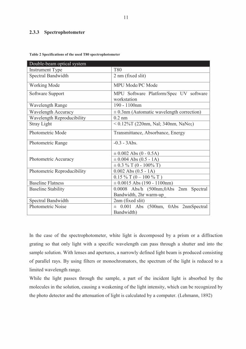
11
233 Spectrophotometer
Table 2 Specifications of the used T80 spectrophotometer
Double-beam optical system Instrument Type T80 Spectral Bandwidth 2 nm (fixed slit)
Working Mode MPU ModePC Mode
Software Support MPU Software PlatformSpec UV software workstation
Wavelength Range 190 - 1100nm Wavelength Accuracy plusmn 03nm (Automatic wavelength correction) Wavelength Reproducibility 02 nm Stray Light lt 012T (220nm Nal 340nm NaNo2)
Photometric Mode Transmittance Absorbance Energy
Photometric Range -03 - 3Abs
Photometric Accuracy
plusmn 0002 Abs (0 - 05A) plusmn 0004 Abs (05 - 1A) plusmn 03 T (0 - 100 T)
Photometric Reproducibility 0002 Abs (05 - 1A) 015 T (0 ndash 100 T )
Baseline Flatness plusmn 00015 Abs (190 - 1100nm) Baseline Stability 00008 Absh (500nm0Abs 2nm Spectral
Bandwidth 2hr warm-up_ Spectral Bandwidth 2nm (fixed slit) Photometric Noise plusmn 0001 Abs (500nm 0Abs 2nmSpectral
Bandwidth)
In the case of the spectrophotometer white light is decomposed by a prism or a diffraction
grating so that only light with a specific wavelength can pass through a shutter and into the
sample solution With lenses and apertures a narrowly defined light beam is produced consisting
of parallel rays By using filters or monochromators the spectrum of the light is reduced to a
limited wavelength range
While the light passes through the sample a part of the incident light is absorbed by the
molecules in the solution causing a weakening of the light intensity which can be recognized by
the photo detector and the attenuation of light is calculated by a computer (Lehmann 1892)
12
The light attenuation is a measurement of the absorption of light and is therefore a measurement
of the concentration of the absorbing molecules in the analyzed solution In this way the
concentration of the substance can be determined using the Lambert-Beer law or a calibration
curve (Boumlcker 1979)
The final aim of the measurement is the detection of the attenuation of the light intensity by the
substance in the measuring cell The measurement result depends on the brightness of the light
source (L) and the sensitivity of the photodetector (Ph) However the properties of these
components change under the influence of fluctuations in the supply voltage temperature and
aging The single-beam therefore is not stable in the long run and must be frequently
recalibrated (wwwphotometercom 2014)
This may be justifiable for individual measurements in the laboratory but in the context of
industrial settings continuous measurement influences of the light source fluctuations have to be
eliminated This leads to the dual-beam method
Figure 4 Structure of a photometer with a dual-bean (wwwphotometercom 2014)
Here a semi-transparent mirror splits the ray into two beams a measurement beam (M) which
passes through the sample and impinges on a first photodetector and a reference beam (V) which
falls directly on a second receiver
The measured value is created by forming a ratio so that the variations in the luminosity of the
light source have no effect However a remaining error source is the change in the sensitivity of
the two photodetectors Therefore the optimum solution is to use two beams and only one
photoreceptor During the project an UVVIS Spectrophomater (model T80 from PG Insturments
Ltd) was used which works exactly in the described manner
13
Figure 5 Dual beam measuring method with only one photodetector (wwwphotometercom 2014)
Again the measured value is created by calculating the ratio of the sample and reference beams
Due to a rotating disc profile (Chopper) the two beams alternate on the same photo detector This
eliminates not only the variations in the light source but also changes of sensitivity of the
photoreceptor are eliminated (Spektrum 1999)
24 Fluorimeter
Table 3 Specifications of the used FluoroMaxR Fluorimeter
FluoroMaxR-4 with USB von HORIBA Lamp Vertically mounted CW 150 W Ozone-free xenon
arc lamp Gratings 1200 groovemm blazed at 330 nm (excitation) and
500 nm (emission) plane ruled Detectors Emission R928P photon counting PMT (185-850
nm) and reference photodiode for monitoring lamp output
Water Raman SN 60001 (RMS method) See Signal-to-noise ratio Slits Continuously variable from 0 to 30 nm Accuracy 05 nm Repeatability 01 nm Minimum step 00525 nm Integration time 0001 to 160 sec Software FluorEssence Monochromators Automatic self-calibration of all wavelength drives
and slits All reflective optics Czerny-Turner spectrometers
Spectral Correction Factors Included
14
Fluorometry is a molecule-spectroscopic analysis that utilizes the property of electronically
excited molecules to emit the absorbed excitation energy as luminescence radiation Since the
electronic excitation of the molecules take place by absorption of light fluorimetry is a
photoluminecense method It finds versatile applications in both organic and inorganic analysis
The outstanding features of this method are their high selectivity and high sensitivity (Zander
1981)
The process is characterized particularly by some features At first it is a direct photometric
method for qualitative and quantitative analysis It is highly sensitive and has a wide range of
linearity Furthermore there are small amounts of material required for the analysis Online as
well as in-situ analysis are possible Lastly there is no or little sample preparations required
which leads to a non-destructive procedure That means the sample can be returned without
problems (Zander 1981)
Fluorimetry is generally based on the detection of emitted luminescent radiation from a sample
or a photochemical mediator molecule (fluorescent marker)
Luminescence radiation arises when electrons move from a higher to a lower orbital This is
called Stokes shift Stokes fluorescence is the re-emission of longer wavelength photons (lower
frequency or energy) by a molecule that has absorbed photons of shorter wavelengths (higher
frequency or energy) It is characteristic for every substance (Schmidt 2000)
A prevention of fluorescence by other types of dissipation of the excitation energy may occur
For instance an energy transfer to other molecules without radiation (eg photosynthesis) or
internal conversion
The intensity of the fluorescence of a solution depends on the intensity of the excitation light
(Iα) the molar absorption coefficient ε of the fluorescent substance the concentration c of the
sample and the quantum yield Q
I0 ndash intensity of emitted light
Ia ndash intensity of attenuated light
15
c ndash Concentration of sample
d ndash Distance of the light or sample diameter
ε ndash molar absorption coefficient
Fluorimetry is used especially often in the field of quantitative analysis because in this case the
detection sensitivity is much higher than for pure absorption photometry The reason is the ratio
of the absorption photometry where usually slightly different signals are measured (Boumlcker
1979)
The majority of chemical compounds have a fluorescence ability Almost all aromatic
hydrocarbons are characterized by fluorescence assets Nevertheless the introduction of
substituents derogates this Particularly nitro and carboxylic acid as well SH-groups and related
substituents almost completely delate the fluorescence (Schmidt 2000)
Fluorimetry has a high detection limit of 10-12 Mol whereas in the absorption analysis only up
to 10-8 Mol can be detected At high substrate concentrations attention should be paid to the fact
that the fluorescence intensity Q is no longer a linear function of the concentration c To stay in
the linear range a maximum concentration of should not be exceeded In the following
figure the structure of a fluorimeter device is presented
Figure 6 Common structure of a fluorimeter device (Rouilly 2014)
16
Mercury or xenon lamps are often used as sources of excitation light Mercury vapor lamps emit
a line spectrum with high intensities in the lines (at 254 313 36566 405 546 577 630 nm )
via a low-intensity continuous background Xenon lamps have a continuous emission spectrum
but its intensity decreases in the UV range
Important properties of monochromators are their light intensity the spectral slit width and the
freedom of scattered light In modern appliances imaging holographic gratings are used All
optical elements such as lenses gratings mirrors and beam splitters influenced by their spectral
characteristics influence the intensity and polarization of the reflected and transmitted radiation
as a function of wavelength
Photomultiplier are used as which allow due to their high amplification (106 to 108) the
measuring of lower light intensities up to single photons Depending on the material of the
photocathode different types of photoreceptors can vary in terms of their absolute and spectral
sensitivities The gain of the photomultiplier depends on the applied voltage (Zander 1981)
25 Prototype
The instrument which was used for this project was designed to measure and analyze samples of
microalgae by using the method of a fluorimeter In line with the idea of inexpensive production
the construction is relatively basic A schematic diagram is presented in the graphic below
Figure 7 schematic diagram of the prototype sensor (left) and photo (right) (Rolim Heinen amp Huff 2014)
17
As is shown above the installation is similar to the fluorimeter (qv figure 6) The main
components are an LED light source which sends a light beam into an opaque chamber where
the sample is placed and two optical receptors which are positioned at angles of 180deg and 90deg
In contrast to the fluorimeter only one filter is used here (in the fluorimeter three mochrometers
were used) The filter works in the same manner as the monochrometer and blocks all unwanted
wavelengths so that just one specific or particular spectrum can pass through
Figure 8 Filter ldquoStrawrdquo to eliminate unwished wave length
The filter absorbs undesired wavelengths between 300 and 400 nm but has a transmission of 88
in case of the important spectrum (lt 400 nm) which is not optimal but a calculable factor
since itrsquos the same loss in any sample and series of tests
Even though lasers have excellent characteristics in case of accuracy and wavelength they are
relatively expensive In opposition to LEDs In opposition to LEDs Caused by that an LED light
source is installed together with the two optical sensors The high potency LED lamp emits a
blue light beam which fits well with the potential spectrum of absorbance of the chlorophyll and
should provide optimal requirements for the microalgae
18
26 Measurement of Biomass
The analyses of the biomass provides information about growth rate and as a consequence
thereof biological activity Therefore a vacuum pressure pump was used together with paper
filters with a diameter of 205 μm and a pore size of 14 μm
A sample of 50 ml was taken from the batches and filtered through the paper (weighted before)
while the vacuum pump supported the passaging of the liquid Afterwards the nearly-dry paper
was stored in an oven at 60 degC for approximately 24 hours The mass difference gives some
indication of the amount of biomass in the 50 ml solution
27 Measurement of Chlorophyll
An issue in chlorophyll measurement is extracting the pigments from the cells Therefore a
sample of 10 ml is filtered (same procedure as for biomass) The extract is stored afterwards in a
90 acetone solution at 4 degC for approximately 24 hours Acetone is a moderate polar solvent
which is after methanol the best solution for chlorophyll pigments because it consists of polar
areas as well as a lipophilic phytel rest (see figure 9) (Lourenccedilo 2006)
Figure 9 Chemical structure of chlorophyll (Willows 2013)
19
Due to the reference (Lourenccedilo 2006) the solution should be centrifuged for around 10 minutes
and 3000 rpm This strategy is used because usually the filter is cut in pieces before stored in the
tube to guarantee a better detachment of the chlorophyll The pre-tests have shown that the
results are more accurate when the filter isnrsquot cut but rolled up and put into the tube (filtrate
towards the tubes inside) If than filled carefully up with acetone (washing out of the extract
must be avoided during infusion) the extraction of chlorophyll will be optimal without the
problem of filter rests and other cell bodies
In a further step the chlorophyllacetone solution is measured in a spectrophotometer by 630 nm
647 nm and 663 - 665 nm The amount of chlorophyll is calculated by the following statistic
equations from Lourenccedilo (2006)
D663-665 D647 D630 ndash absorbance at the wavelength Dx after correction by the cell-to-cell blank and subtraction of the cell-to-cell blank corrected absorbance at 750nm
l - Cell (cuvette) length [cm] = 1
v - Volume of acetone [ml] = 10
V - Volume of filtered water [l] = 10
Accordingly the term That simplifies the equations
20
3 Results and discussion
During the project the algae suspension was scanned over a time interval of 10 days plus one
day incubation During this time the batches were subjected to various light conditions (Batch A
= 4000 Lux Batch B = 5500 Lux Batch C = 7000 Lux Batch D = 8500 Lux Batch E = 10000
Lux) This was performed to analyze the effect of different light intensity on algae and
accumulation of chlorophyll To obtain useful results it is essential to eliminate as much
unwished problems as possible According to this the growing of the algae was analyzed at first
because any discrepancies of the algae growth would lead to consequential errors in case of
chlorophyll tests
31 Algae growth The growth of Scanedesmus Sp was measured via spectrophotometer and biomass dry weight
Optical density of biomass was determined at 750 nm One ml of the sample batch was taken and
measured in a spectrum between 400 nm and 750 nm
Usually the growth of an algae culture follows certain steps It starts with the lag phase (1)
followed by an exponential phase (2) The culture growth will reach a point of overpopulation in
which one or more essential resources are limited Growth and death rate are either in
equilibrium or the cells already stopped the proliferation This is called the stationary phase (4)
At the end the living conditions are so bad that the cell population starts to decrease rapidly
(usually caused by a deficiency of important nutrients) The last phase is called death phase (5)
Figure 10 Sketch of algae growth dynamics
21
The before explained growth dynamic differs to the culture development during the test Figure 7
(below) presents all graphs (of absorbance [400hellip750 nm]) of the five batches in a time interval
of ten days So in total 50 single graphs summarized in that 3D - graphic It gives an interesting
overview of the total experiment
Figure 11 Progress of all 5 batches in a time interval of 11 days
In the figure a formation can be seen that looks like one side of a steep ridge that starts relatively
flat in the beginning and becomes steeper in the posterior tier Rifts in the formation are caused
by some problems associated with the spectrophotometer at certain wavelengths Following the
observation that the results are the same regardless of the kind of sample analyzed the
assumption that the spectrophotometer doesnrsquot work at these wave length may be accepted
Furthermore a pattern of wave formations is recognizable Every wave formation has a
maximum at around 400 nm and 480 nm and between 650 nm and 670 nm The first ldquowaverdquo is
the result of the batch analyses from the first day the second from the second day and so on
The wavelike formation is caused by the differential growth of the algae under different light
22
conditions The most exposed batch (E) already has a higher algae concentration on dayx as
compared to the lowest exposed batch (A) one day after
Figure 12 By comparison absorbance between 400 nm and 750 nm of five batches at day 6 and 72
The first figure curvebatch E has the highest absorbance starting between 06 and 065 at 400
nm and ending up at the second maximum at around 059 In comparison batchcurve A from
one day after also starts between 06 and 065 but falls under the values of Batch E at the second
maximum which occurs at around 056 This is responsible for the wave effect between the
days Only at the last day does Batch A exceed the high peaks of Batch E from the previous day
This is caused by the beginning of the exponential phase Unfortunately the cultures did not pass
through all four phases as expected The exponential phase started between day 7 and 9
depending on the Batch
2 The days are chosen randomly to proof the above delineated statement The same course of curves could be confirmed for every day Just the intensity of absorbance varies
23
We can see the effect of light between the different figures The culture of Batch E already began
exponential growth at day 7 while the lag phase in Batch A persisted until the 8th9th day
Figure 13 Progress of culture growth comparing Batch E (left) and A (right) during the 10 days in comparison to the Absorbance
The following statements can be made to summarize the observed algae growth Since the
different colonies in the Batches react to the light intensity as expected the assertion can be
made that the Biomass (mB) of
When comparing the results of the optical density with the gravimetric measurements some
issues have to be mentioned The dry weight measurement was only performed after day four
because the amount of biomass measured before day five was considered too small to be reliably
assessed Even after the fifth day some unexpected changes in the curve shape were visible
Nonetheless the main shape of the curve approximates an exponential slope after day eight
which is consistent with the measurement of the optical density
24
Figure 14 Dry weight (mgl) of Scenedesmus Sp for 10 days grown under different light conditions
In addition the amount of biomass increases daily in every Batch according to the results of the
optical density
This is not so in the case of the dry weight measurement where no decipherable pattern can be
determined for the first half of the test period Some problems occurred during the laboratory
processing including the malfunctioning of an oven during day 6 and a restoration of the
samples during day seven Additionally as a consequence of the high error-proneness of the
earlier dry weight analysis due to the use of relatively small volumes findings from the dry
weight analyses should be considered with caution
Beyond these issues it has to be mentioned that the colonies didnrsquot reach the stationary phase
and thus also failed reach the death phase These two statuses of the growth dynamic could
have been interesting for the comparison of the algaechlorophyll ratio while exposed to different
light intensities
25
The results of biomass and spectrophotometer analyses confirm the findings of the designed
prototype in the way that the order of the batches in proportion to dissolved substances (
biomass) is the same as the order of the Batches themselves (BA lt BB lt BC lt BD lt BE dayx)
Figure 15 Algae development measured by prototype during the days 7 - 11 plotted as a function of voltage
The figure above shows the general light intensity that passes through the sample filled with
water (~ 245 V) The larger the amount of dissolved material in the sample the less light will
pass through it and consequently the lower the measured voltage will be With a general
tendency toward a lower voltage a larger amount of biomass can be ascertained but it has to be
mentioned that no statements about the type of curve shape can be made Unfortunately more
test results would have been necessary to make further statements
0
05
1
15
2
25
3
7 8 9 10 11
Outp
ut vo
ltage
at 1
80deg(
V)
Days
A
B
C
D
E
Water
26
32 Chlorophyll formation
After the chlorophyll-acetone mix is stored for 24 hours it is analyzed with a spectrophotometer
For the calculation of chlorophyll content according to Jeffrey amp Humphrey (1975) only some
wavelengths are important Nevertheless the chlorophyll was treated in the same way as the
algae and measurements were made in the range of 400 nm to 750 nm in order to determine
possible similarities
Figure 16 Chlorophyll (mgl) of Scenedesmus sp for 10 days grown under different illumination conditions
The concentration of total chlorophyll increases during the test The results show a steady growth
if expressed as the exponential regression curve (dotted lines) for Batches D and E (R = 09) A
better correlation is shown for a linear regression for Batches A and B (R = 09 instead of 076)
Batch C doesnrsquot show a strong correlation under either a linear (R = 072) or an exponential
growth (R = 076) assumption Many factors affect the results of the Chlorophyll measurement
Firstly the analyses are susceptible to mistakes made during the processing When removing 10
ml from the batches with a concentration of barely 1 mgL and using those samples in a cuvette
of 3 mL the amount of Chlorophyll is typically in a range of 0 ndash 10 μgmL Working with such
small quantities can lead to inaccuracies during processing in addition to errors made on behalf
of the measuring engine itself
Rsup2 = 07602
Rsup2 = 07602
Rsup2 = 09004
Rsup2 = 09037
Rsup2 = 07594
0
05
1
15
2
25
0 1 2 3 4 5 6 7 8 9 10 11
Chlo
roph
yll a
+b (m
gl)
Day
C
D
E
B
A
Expon (C)
Expon (C)
Expon (C)
Expon (D)
Expon (D)
Expon (E)
Linear (B)
Expon (A)
Linear (A)
27
Nevertheless we can make the assumption that the tendency (daily increase) makes sense The
results of the pilot engine show slightly decreasing curves At day 8 there is an obvious mistake
to declare This is not visible with regard to algae measurement at day 93 This leads to the
assumption of a mistake made during the preparing procedure with acetone Since the
abnormality can be found in all batches a mistake during the withdrawal can be ruled out
Figure 17 Chlorophyll development during the days 7 - 11 plotted as a function of voltage
A further problem is that the curves are not clearly separable They cross each other without
showing a decipherable trend with regard to which batch has the highest or the lowest
translucency (which would be proportional to the voltage) As a consequence these results
cannot provide information about the effect of different light irradiation and it is questionable
whether they can be used to make an assumption about chlorophyll accumulation
3 The spectrophotometer analyzes of chlorophyll is one day after due to the 24 hours storing of the samples
0
05
1
15
2
25
3
7 8 9 10 11
Outp
ut vo
ltage
at 1
80deg(
V)
Days
E
B
C
D
A
Water
28
33 Correlation of Algae and Chlorophyll growth The main rationale for using different light irradiation for the Batches was to determine the
relationship between algae growth and the Chlorophyll enhancement Hence interest lay beyond
simply examining the thesis that the concentration of Chlorophyll is directly linked to the algae
growth Furthermore there was interest in exploring whether a specific relationship existed
between the algae growth rate the exposure to light and the amount of chlorophyll produced
Figure 18 Collocation of AlgaeChlorophyll absorbance (by 665 nm) by a spectrophotometer for 11 days
Unfortunately an incomplete test phase (no algae growth until the stationary phase) was
responsible for a lack of results that could be used for further analysis Nevertheless the ratio of
Chlorophyll-to-Algae growth shows a decent progression (see also Table 4) There is no
evidence for a similar progression if the tests proceed for one or two weeks In theory the
chlorophyll concentration should increase more rapidly in the exponential phase (until now the
progress is best described as a linear growth) Furthermore the concentration of algae as well as
of chlorophyll from batch E should reach its maximum first followed by batch D C B A (in
this order) and continue at a stationary rate
BAA
lgae
BAC
hlBB
Alg
aeBB
Chl
BCA
lgae
BCC
hl
BDA
lgae
BDC
hl
BEA
lgae
BEC
hl
002040608
112141618
12
34
56
78
9 1011
BatchSubstrate
Abso
rban
ce
Days
BAAlgae
BAChl
BBAlgae
BBChl
BCAlgae
BCChl
BDAlgae
BDChl
BEAlgae
BEChl
29
Due to the issues described in the earlier chapters the results from analyses on biomass are less
convincing than those arising from the analyses of the spectrophotometer In addition and
contrary to the absorbance measurement the values of dry weight and calculated chlorophyll
correlate weakly in cases of batches with higher light saturation This may be due to inaccuracies
from the dry weight results or another reason could be the earlier start of a kind of exponential
growth for the chlorophyll while the results for the biomass donrsquot show an exponential increase
until the 7th day
Table 4 Overview of the results of biomass prototype and spectrophotometer analyzes
Substrate Biomass (mgl) ndash Dry weight and Chl Optical density (V) -
Prototype Absorbance - Spectrophotometer
Min Max R Min Max R Min Max R BAAlgae 146 327
092 185 061
- 013 156
094 BAChl 001 164 212 170 001 017 BBAlgae 154 444
085 124 049
- 013 169
089 BBChl 004 172 206 175 001 026 BCAlgae 170 478
078 097 042
- 012 170
082 BCChl 002 188 194 181 001 023 BDAlgae 162 504
068 104 044
- 011 172
094 BDChl 002 124 196 171 001 026 BEAlgae 160 515
066 130 035
- 009 175
097 BEChl 002 114 215 195 001 031 The less exciting results are unfortunately given by the Prototype Here no significant correlation
can be mentioned at all In contrast to the spectrophotometer these values are provided by the
direct transmission Therefore the highest solution has the lowest value because more light is
absorbed by the dissolved material which is in this case biomass (or pure chlorophyll) This
result is surprisingly disappointing because the tests performed beforehand with fluorescence
(realized by Leonardo M Rolim) show a straight dependency of proportional relationship
between percental solution and transmission (see Figure 19 below)
Fluorescein is a fluorescent dye from the group of the xanthene It was used for the previous tests
because itrsquos a non-biological and well known substance with which all unwished side effects of a
living system can be avoided during tests
30
Figure 19 Measuring points of concentration given in optical density from fluorescence (Rolim Heinen amp Huff 2014)
The graph shows the transmission by 180 degC as accomplished with the algae and chlorophyll
during this work The curve suggests a negative exponential trend This was also expected for the
new series of tests While a clear difference can be recorded in the case of fluorescein the values
of chlorophyll almost didnrsquot change This could be an effect of the high fluorescent impact of
fluorescence Due to the growth rate of chlorophyll (see Table 4 Chl Min and Max) which goes
from 001 gmL up to almost 18 gmL (180 times more) compared with the fluorescence which
goes from 001 gmL up to 03 gmL (30 times more) this is questionable since the concentration
difference is 5 times higher for pure chlorophyll a fluorescent pigment as well but the effect is
very little Nevertheless it could be an indication as to why results from the test were not as
expected
The analyses by the fluorimeter provides further interesting results The figure below presents
the results of chlorophyll for the 11th day The x-axis shows the input of the wave length
produced by the laser The excitation is visible on the y-axis while curves on the graph present
one specific wave length each between 400 and 800 nm (with an interval of 5 ie a new
measurement was performed for every 5 nm) In order to simplify the graphical presentation the
legend was omitted
31
Figure 20 Display of emission and excitation measured by the fluorimeter of day 11 for chlorophyll
The figure provides an important insight into the behavior of chlorophyll fluorescent The
formation on the bluish part of the light spectrum (270 ndash 430 nm) and the second cluster of peaks
between 650 and 675 nm are quite revealing The table below explains the most important
curves
Table 5 Legend of figure 16
Color wave length (nm) red 675 blue 670 gray 680
light green 665 orange 685
light blue 660 dark blue 690 dark green 695
These eight curves are explicitly mentioned because they have the highest response in the tested
emission spectrum Due to usually low concentrations of samples eg chlorophyll in μgml a
high response is vital The results of the other test days are equal They simply vary in the height
of excitation as a result of a higher concentration
0
200000
400000
600000
800000
1000000
1200000
1400000
1600000
300 325 350 375 400 425 450 475 500 525 550 575 600 625 650 675 700 725 750
Exita
tion
ampe
rage
at 9
0deg(m
A)
Emission wave lenght (nm)
32
Figure 21 Display of emission and excitation measured by the fluorimeter between the days 0 and 11 for chlorophyll (BA)
The daily difference of the excitation is presented above The course of the curves is equal and
just differs as mentioned before in the amount of ampere measured by the receptor The same
shape would be plotted by the other batches The only difference again would be the level of
excitation
The progression of the chlorophyll curves during the tests shows a permanent increase beginning
at day three An exponential correlation can be verified for the plotted curves Thus the results
from the fluorimeter are as expected before Still the problem as mentioned before of the
incomplete growth of the algae was responsible for a lack of further information which could
have been interesting
0
200000
400000
600000
800000
1000000
1200000
350 375 400 425 450 475 500 525 550 575 600 625 650 675 700 725 750
Excit
atio
n am
pera
ge a
t 90
deg(m
A)
Emission wave lenght (nm)
0
1
2
3
4
5
6
7
8
9
10
11
33
Figure 22 Trend of the chlorophyll excitation peaks during 11 days measured by the fluorimeter
In the following section the results from the algae analyses are explained One problem has to be
mentioned beforehand
The graph below shows the outcome from the last day Highly overlapping curves are visible
This is not caused by fluorescence but by the reflection of each wave length itself due to a high
solution The analyses made by the fluorimeter requires at least 30 minutes That it enough time
for the dissolved particle to settle down The x-axis can accordingly be viewed as a timeline
scale As more time passes by the reflection impact reduces
Rsup2 = 08453
0
200000
400000
600000
800000
1000000
1200000
1400000
1600000
1800000
2000000
0 2 4 6 8 10 12
Excit
atio
n am
pera
ge a
t 90
deg(m
A)
Days
660
665
430
405
375
Log (375)
34
Figure 23 Fluorimeter results of algae (BA day11)4
When the y-axis is limited to 100000 mA some other formations are visible Interestingly they
have the same shape as the curves of the chlorophyll which leads to the assumption that those
overlapped curves are indeed the fluorescent impact of the chlorophyll pigments
4 Every curve presents one wave length of the emission spectrum in an interval of five The legend is once more excluded due to a better overview
0
1000000
2000000
3000000
4000000
5000000
6000000
7000000
8000000
300 325 350 375 400 425 450 475 500 525 550 575 600 625 650 675 700 725 750
Excit
atio
n am
pera
ge a
t 90deg
(mA)
Emission wave lenght (nm)
35
Figure 24 Fluorimeter results of algae (BA day11) with limited y-axes up to 100000 mA5
On closer examination it can be interpreted that the higher curves (blue orange green dark
blue redhellip) are the same wavelengths as seen in the Table 5 Legend of figure 16rdquo The highest
response again is at 675 nm Measureing by a different wave length than 675 nm will cause
lower excitation The same happens in case of chlorophyll
The excitation is low in comparison with the results of the pure chlorophyll because the
chlorophyll is not separated from the cells which hinders the light from reaching the pigments
in addition to leaving the sample and stimulating the receptor
The comparison with the other batches and the analyses of the different days provides the same
results as for the chlorophyll That means the Excitation of BA(dx) lt BB(dx) lt BC(dx) lt BD(dx)
lt BE(dx) and the Excitation of BA(dx) lt BA(dx+1) BB(dx) lt BB(dx+1) BC(dx) lt BC(dx+1)
BD(dx) lt BD(dx+1) BE(dx) lt BE(dx+1)
5 The legend is once more excluded due to a better overview
0
10000
20000
30000
40000
50000
60000
70000
80000
90000
100000
300 325 350 375 400 425 450 475 500 525 550 575 600 625 650 675 700 725 750
Excit
atio
n am
pera
ge a
t 90
deg(m
A)
Emission wave lenght (nm)
36
4 Conclusiones
According to the results from the fluorimeter the algae growth and chlorophyll enhancement
appear to be as expected This leads to the question as to why the previous tests donrsquot have
similar outcomes The answer to this question and the reason why fluorimeters are used for low
quantities is the same They have a very high accuracy and are thus extremely efficient even
for low quantities Nevertheless they are extremely expensive and the main task of this project
was to determine whether it was possible to measure chlorophyll (pure or even intracellular) with
the prototype or if not to work out further steps for the development of the engine
The first step apart from the biological section is to make the engine more stable During the
project problems often occurred with regard to replication of results because small changes in the
electrical connection contributed to different outcomes while using the same sample This made
the testing more complicated and made unnecessary repetitions of measurement indispensable A
shell for the entire construction in which the electronic is fixed should solve this problem An
extension cable which leads to the measuring box together with a smaller diameter of the cell
itself would also be useful The laser and the two receptors should be installed separately from
the cell and waterproofed (plastic and glue should be sufficient) As a result the cell could be
introduced into a sample to measure which not only simplifies the procedure but it is also closer
to any practical application
The next action is the acquisition of the correct optical filter The results of the fluorimeter
suggest an optimal emission at 430 plusmn 10 nm while the excitation should be measured at 675 plusmn 10
nm The closer the measurement is to these wavelengths the higher the values of the results
Furthermore it was explained how other wave lengths overlap the fluorescence effect This can
be avoided by use of at least two filters one which filters the light of the laser and blocks out
every wavelength except for those in the range of eg 420 ndash 440 nm and a second filter which
allows for only the spectrum from 665 to 685 nm to pass
Nevertheless an upgrade of either the receptor or laser but probably both will be inevitable As
mentioned in the previous chapter the outcome of the 90deg measurement for algae and
chlorophyll is almost zero In actuality it has the same value as if measured with water which
means that the receptor is not able to recognize any approaching light On the other hand it may
37
be that the laser is too weak so that not enough light is injected In any case adjustment for the
right filter range should be the first step
When the filter and laserreceptor problems are solved a new test with fluorescence would make
sense At this stage it is important not only that the results are good for one series of tests but
also that they are repeatable Daily calibration of the engine is not only effortful and time-
consuming but it can also lead to variable results After good and stable results are achieved
with fluoresce a new test series with algae can be started Therefore it would be useful to create
a serial dilution of an algae culture which is already in the stationary phase and highly
concentrated If the results are suitable it can be continued with a serial dilution of those algae
Even if the results from the 90deg measurement are not satisfying a further test with pure
chlorophyll could be accomplished on condition that the results from the 180deg measurement are
decent
Only after all the described experiments have sufficient results should a new long-term test series
be started For this purpose no more than three batches should be installed with an intensity of
illumination between 3000 and 10000 lux The test duration should be approximately 30 days to
ensure that the culture passes through all growing and dying phases Tests performed with the
spectrophotometer can indicate a change of the growing conditions so that further and more
elaborated tests with the fluorimeter and biomass can be performed The measurement of
biomass should be sufficient if performed every three days (a daily testing during the exponential
phase would perhaps be useful) By using the fluorimeter care has to be taken so that the dilution
of the sample is large enough otherwise overlapping effects occur The analyses with the sensor
should be performed daily in order to get a consistent overview of the chlorophyllalgae ratio as
well as to gauge the accuracy of the sensor
38
5 Bibliography Boumlcker J (1979) Spektroskopie Instrumentelle Analytik mit Atom- und Molekuumllspektroskopie
(1 Edition Ausg) Wuumlrzburg Vogel Verlag und Druck GmbH amp Co
Hegewald P (2006) Scenedesmusndashlike algae of Ukraine Tsarenko E amp B Braband
Lehmann E W (1892) Uumlber ein Photometer Erlangen
Lourenccedilo S (2006) Cultivo de Microalgas Marinhas Princiacutepios e Aplicaccedilotildees
Luumlrling M (1999) The Smell of Water Grazer-Induced Colony Formation in Scenedesmus
Wageningen Pulz und Gross
Mills I Cvitaš T Homann K Kallay N amp Kuchitsu K (1993) Quantities Units and
Symbols in Physical Chemistry (Green Book)
Rolim L M Heinen A L amp Huff D D (2014) Desenvolvimento de sensor oacuteptico portaacutetil
para mediccedilatildeoes online de concentraccedilatildeo no cultivo de microalgas Porto Alegre
Rouilly V (2014) Schmidt W (2000) Optische Spektroskopie (Bd 2 Edition) Weinheim
WILEY-VCH Verlag GmbH
Unknown (1999) Photometer Spektrum Akademischer Verlag
Willows R D (2013) Structure of chlorophyll Organic Letters
Zander M (1981) Fluorimetrie Berlin-Heidelberg-New York Springer-Verlag
Internet sources Openwetwareorg
photometercom
teachingshuacuk
wikipediaorg
39
6 List of figures Figure 1 Pilot batch deployment 7
Figure 2 Relation between transmittance and absorbance 9
Figure 3 Structure of a photometer 10
Figure 4 Structure of a photometer with a dual-bean 12
Figure 5 Dual beam measuring method with only one photodetector 13
Figure 6 Common structure of a fluorimeter device 15
Figure 7 schematic diagram of the prototype sensor (left) and photo (right) 16
Figure 8 Filter ldquoStrawrdquo to eliminate unwished wave length 17
Figure 9 Chemical structure of chlorophyll 18
Figure 10 Sketch of algae growth dynamics 20
Figure 11 Progress of all 5 batches in a time interval of 11 days 21
Figure 13 By comparison absorbance between 400 nm and 750 nm of five batches at day 6 and 7
22
Figure 14 Progress of culture growth comparing Batch E (left) and A (right) during the 10 days
in comparison to the Absorbance 23
Figure 15 Dry weight (mgl) of Scenedesmus Sp for 10 days grown under different light
conditions 24
Figure 16 Algae development measured by prototype during the days 7 - 11 plotted as a function
of voltage 25
Figure 17 Chlorophyll (mgl) of Scenedesmus sp for 10 days grown under different illumination
conditions 26
Figure 18 Chlorophyll development during the days 7 - 11 plotted as a function of voltage 27
Figure 19 Collocation of AlgaeChlorophyll absorbance (by 665 nm) by a spectrophotometer for
11 days 28
Figure 20 Measuring points of concentration given in optical density from fluorescence 30
Figure 21 Display of emission and excitation measured by the fluorimeter of day 11 for
chlorophyll 31
Figure 22 Display of emission and excitation measured by the fluorimeter between the days 0
and 11 for chlorophyll (BA) 32
Figure 23 Trend of the chlorophyll excitation peaks during 11 days measured by the fluorimeter
33
Figure 24 Fluorimeter results of algae (BA day11) 34
Figure 25 Fluorimeter results of algae (BA day11) with limited y-axes up to 100000 mA 35
40
7 List of tables Table 1 Composition of algae supplementary medium 6
Table 2 Specifications of the used T80 spectrophotometer 11
Table 3 Specifications of the used FluoroMaxR Fluorimeter 13
Table 4 Overview of the results of biomass prototype and spectrophotometer analyzes 29
Table 5 Legend of figure 16 31
41
Declaration of Authorship I hereby certify that this work has been composed by me and is based on my own work
unless stated otherwise No other person`s work has been used without due
acknowledgement in this report All references and verbatim extracts have been quoted
and all sources of information including graphs and data sets have been specifically
acknowledged
______________________ ________________________ Ort Datum Signature
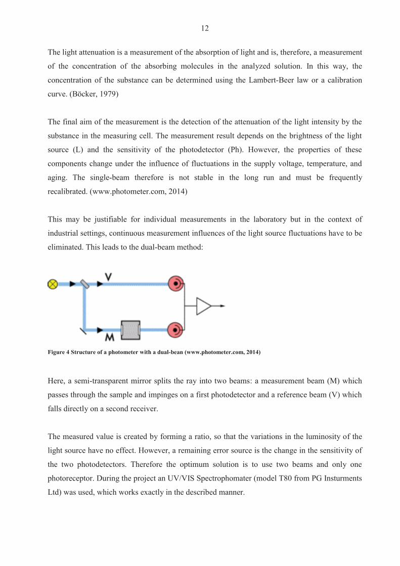
12
The light attenuation is a measurement of the absorption of light and is therefore a measurement
of the concentration of the absorbing molecules in the analyzed solution In this way the
concentration of the substance can be determined using the Lambert-Beer law or a calibration
curve (Boumlcker 1979)
The final aim of the measurement is the detection of the attenuation of the light intensity by the
substance in the measuring cell The measurement result depends on the brightness of the light
source (L) and the sensitivity of the photodetector (Ph) However the properties of these
components change under the influence of fluctuations in the supply voltage temperature and
aging The single-beam therefore is not stable in the long run and must be frequently
recalibrated (wwwphotometercom 2014)
This may be justifiable for individual measurements in the laboratory but in the context of
industrial settings continuous measurement influences of the light source fluctuations have to be
eliminated This leads to the dual-beam method
Figure 4 Structure of a photometer with a dual-bean (wwwphotometercom 2014)
Here a semi-transparent mirror splits the ray into two beams a measurement beam (M) which
passes through the sample and impinges on a first photodetector and a reference beam (V) which
falls directly on a second receiver
The measured value is created by forming a ratio so that the variations in the luminosity of the
light source have no effect However a remaining error source is the change in the sensitivity of
the two photodetectors Therefore the optimum solution is to use two beams and only one
photoreceptor During the project an UVVIS Spectrophomater (model T80 from PG Insturments
Ltd) was used which works exactly in the described manner
13
Figure 5 Dual beam measuring method with only one photodetector (wwwphotometercom 2014)
Again the measured value is created by calculating the ratio of the sample and reference beams
Due to a rotating disc profile (Chopper) the two beams alternate on the same photo detector This
eliminates not only the variations in the light source but also changes of sensitivity of the
photoreceptor are eliminated (Spektrum 1999)
24 Fluorimeter
Table 3 Specifications of the used FluoroMaxR Fluorimeter
FluoroMaxR-4 with USB von HORIBA Lamp Vertically mounted CW 150 W Ozone-free xenon
arc lamp Gratings 1200 groovemm blazed at 330 nm (excitation) and
500 nm (emission) plane ruled Detectors Emission R928P photon counting PMT (185-850
nm) and reference photodiode for monitoring lamp output
Water Raman SN 60001 (RMS method) See Signal-to-noise ratio Slits Continuously variable from 0 to 30 nm Accuracy 05 nm Repeatability 01 nm Minimum step 00525 nm Integration time 0001 to 160 sec Software FluorEssence Monochromators Automatic self-calibration of all wavelength drives
and slits All reflective optics Czerny-Turner spectrometers
Spectral Correction Factors Included
14
Fluorometry is a molecule-spectroscopic analysis that utilizes the property of electronically
excited molecules to emit the absorbed excitation energy as luminescence radiation Since the
electronic excitation of the molecules take place by absorption of light fluorimetry is a
photoluminecense method It finds versatile applications in both organic and inorganic analysis
The outstanding features of this method are their high selectivity and high sensitivity (Zander
1981)
The process is characterized particularly by some features At first it is a direct photometric
method for qualitative and quantitative analysis It is highly sensitive and has a wide range of
linearity Furthermore there are small amounts of material required for the analysis Online as
well as in-situ analysis are possible Lastly there is no or little sample preparations required
which leads to a non-destructive procedure That means the sample can be returned without
problems (Zander 1981)
Fluorimetry is generally based on the detection of emitted luminescent radiation from a sample
or a photochemical mediator molecule (fluorescent marker)
Luminescence radiation arises when electrons move from a higher to a lower orbital This is
called Stokes shift Stokes fluorescence is the re-emission of longer wavelength photons (lower
frequency or energy) by a molecule that has absorbed photons of shorter wavelengths (higher
frequency or energy) It is characteristic for every substance (Schmidt 2000)
A prevention of fluorescence by other types of dissipation of the excitation energy may occur
For instance an energy transfer to other molecules without radiation (eg photosynthesis) or
internal conversion
The intensity of the fluorescence of a solution depends on the intensity of the excitation light
(Iα) the molar absorption coefficient ε of the fluorescent substance the concentration c of the
sample and the quantum yield Q
I0 ndash intensity of emitted light
Ia ndash intensity of attenuated light
15
c ndash Concentration of sample
d ndash Distance of the light or sample diameter
ε ndash molar absorption coefficient
Fluorimetry is used especially often in the field of quantitative analysis because in this case the
detection sensitivity is much higher than for pure absorption photometry The reason is the ratio
of the absorption photometry where usually slightly different signals are measured (Boumlcker
1979)
The majority of chemical compounds have a fluorescence ability Almost all aromatic
hydrocarbons are characterized by fluorescence assets Nevertheless the introduction of
substituents derogates this Particularly nitro and carboxylic acid as well SH-groups and related
substituents almost completely delate the fluorescence (Schmidt 2000)
Fluorimetry has a high detection limit of 10-12 Mol whereas in the absorption analysis only up
to 10-8 Mol can be detected At high substrate concentrations attention should be paid to the fact
that the fluorescence intensity Q is no longer a linear function of the concentration c To stay in
the linear range a maximum concentration of should not be exceeded In the following
figure the structure of a fluorimeter device is presented
Figure 6 Common structure of a fluorimeter device (Rouilly 2014)
16
Mercury or xenon lamps are often used as sources of excitation light Mercury vapor lamps emit
a line spectrum with high intensities in the lines (at 254 313 36566 405 546 577 630 nm )
via a low-intensity continuous background Xenon lamps have a continuous emission spectrum
but its intensity decreases in the UV range
Important properties of monochromators are their light intensity the spectral slit width and the
freedom of scattered light In modern appliances imaging holographic gratings are used All
optical elements such as lenses gratings mirrors and beam splitters influenced by their spectral
characteristics influence the intensity and polarization of the reflected and transmitted radiation
as a function of wavelength
Photomultiplier are used as which allow due to their high amplification (106 to 108) the
measuring of lower light intensities up to single photons Depending on the material of the
photocathode different types of photoreceptors can vary in terms of their absolute and spectral
sensitivities The gain of the photomultiplier depends on the applied voltage (Zander 1981)
25 Prototype
The instrument which was used for this project was designed to measure and analyze samples of
microalgae by using the method of a fluorimeter In line with the idea of inexpensive production
the construction is relatively basic A schematic diagram is presented in the graphic below
Figure 7 schematic diagram of the prototype sensor (left) and photo (right) (Rolim Heinen amp Huff 2014)
17
As is shown above the installation is similar to the fluorimeter (qv figure 6) The main
components are an LED light source which sends a light beam into an opaque chamber where
the sample is placed and two optical receptors which are positioned at angles of 180deg and 90deg
In contrast to the fluorimeter only one filter is used here (in the fluorimeter three mochrometers
were used) The filter works in the same manner as the monochrometer and blocks all unwanted
wavelengths so that just one specific or particular spectrum can pass through
Figure 8 Filter ldquoStrawrdquo to eliminate unwished wave length
The filter absorbs undesired wavelengths between 300 and 400 nm but has a transmission of 88
in case of the important spectrum (lt 400 nm) which is not optimal but a calculable factor
since itrsquos the same loss in any sample and series of tests
Even though lasers have excellent characteristics in case of accuracy and wavelength they are
relatively expensive In opposition to LEDs In opposition to LEDs Caused by that an LED light
source is installed together with the two optical sensors The high potency LED lamp emits a
blue light beam which fits well with the potential spectrum of absorbance of the chlorophyll and
should provide optimal requirements for the microalgae
18
26 Measurement of Biomass
The analyses of the biomass provides information about growth rate and as a consequence
thereof biological activity Therefore a vacuum pressure pump was used together with paper
filters with a diameter of 205 μm and a pore size of 14 μm
A sample of 50 ml was taken from the batches and filtered through the paper (weighted before)
while the vacuum pump supported the passaging of the liquid Afterwards the nearly-dry paper
was stored in an oven at 60 degC for approximately 24 hours The mass difference gives some
indication of the amount of biomass in the 50 ml solution
27 Measurement of Chlorophyll
An issue in chlorophyll measurement is extracting the pigments from the cells Therefore a
sample of 10 ml is filtered (same procedure as for biomass) The extract is stored afterwards in a
90 acetone solution at 4 degC for approximately 24 hours Acetone is a moderate polar solvent
which is after methanol the best solution for chlorophyll pigments because it consists of polar
areas as well as a lipophilic phytel rest (see figure 9) (Lourenccedilo 2006)
Figure 9 Chemical structure of chlorophyll (Willows 2013)
19
Due to the reference (Lourenccedilo 2006) the solution should be centrifuged for around 10 minutes
and 3000 rpm This strategy is used because usually the filter is cut in pieces before stored in the
tube to guarantee a better detachment of the chlorophyll The pre-tests have shown that the
results are more accurate when the filter isnrsquot cut but rolled up and put into the tube (filtrate
towards the tubes inside) If than filled carefully up with acetone (washing out of the extract
must be avoided during infusion) the extraction of chlorophyll will be optimal without the
problem of filter rests and other cell bodies
In a further step the chlorophyllacetone solution is measured in a spectrophotometer by 630 nm
647 nm and 663 - 665 nm The amount of chlorophyll is calculated by the following statistic
equations from Lourenccedilo (2006)
D663-665 D647 D630 ndash absorbance at the wavelength Dx after correction by the cell-to-cell blank and subtraction of the cell-to-cell blank corrected absorbance at 750nm
l - Cell (cuvette) length [cm] = 1
v - Volume of acetone [ml] = 10
V - Volume of filtered water [l] = 10
Accordingly the term That simplifies the equations
20
3 Results and discussion
During the project the algae suspension was scanned over a time interval of 10 days plus one
day incubation During this time the batches were subjected to various light conditions (Batch A
= 4000 Lux Batch B = 5500 Lux Batch C = 7000 Lux Batch D = 8500 Lux Batch E = 10000
Lux) This was performed to analyze the effect of different light intensity on algae and
accumulation of chlorophyll To obtain useful results it is essential to eliminate as much
unwished problems as possible According to this the growing of the algae was analyzed at first
because any discrepancies of the algae growth would lead to consequential errors in case of
chlorophyll tests
31 Algae growth The growth of Scanedesmus Sp was measured via spectrophotometer and biomass dry weight
Optical density of biomass was determined at 750 nm One ml of the sample batch was taken and
measured in a spectrum between 400 nm and 750 nm
Usually the growth of an algae culture follows certain steps It starts with the lag phase (1)
followed by an exponential phase (2) The culture growth will reach a point of overpopulation in
which one or more essential resources are limited Growth and death rate are either in
equilibrium or the cells already stopped the proliferation This is called the stationary phase (4)
At the end the living conditions are so bad that the cell population starts to decrease rapidly
(usually caused by a deficiency of important nutrients) The last phase is called death phase (5)
Figure 10 Sketch of algae growth dynamics
21
The before explained growth dynamic differs to the culture development during the test Figure 7
(below) presents all graphs (of absorbance [400hellip750 nm]) of the five batches in a time interval
of ten days So in total 50 single graphs summarized in that 3D - graphic It gives an interesting
overview of the total experiment
Figure 11 Progress of all 5 batches in a time interval of 11 days
In the figure a formation can be seen that looks like one side of a steep ridge that starts relatively
flat in the beginning and becomes steeper in the posterior tier Rifts in the formation are caused
by some problems associated with the spectrophotometer at certain wavelengths Following the
observation that the results are the same regardless of the kind of sample analyzed the
assumption that the spectrophotometer doesnrsquot work at these wave length may be accepted
Furthermore a pattern of wave formations is recognizable Every wave formation has a
maximum at around 400 nm and 480 nm and between 650 nm and 670 nm The first ldquowaverdquo is
the result of the batch analyses from the first day the second from the second day and so on
The wavelike formation is caused by the differential growth of the algae under different light
22
conditions The most exposed batch (E) already has a higher algae concentration on dayx as
compared to the lowest exposed batch (A) one day after
Figure 12 By comparison absorbance between 400 nm and 750 nm of five batches at day 6 and 72
The first figure curvebatch E has the highest absorbance starting between 06 and 065 at 400
nm and ending up at the second maximum at around 059 In comparison batchcurve A from
one day after also starts between 06 and 065 but falls under the values of Batch E at the second
maximum which occurs at around 056 This is responsible for the wave effect between the
days Only at the last day does Batch A exceed the high peaks of Batch E from the previous day
This is caused by the beginning of the exponential phase Unfortunately the cultures did not pass
through all four phases as expected The exponential phase started between day 7 and 9
depending on the Batch
2 The days are chosen randomly to proof the above delineated statement The same course of curves could be confirmed for every day Just the intensity of absorbance varies
23
We can see the effect of light between the different figures The culture of Batch E already began
exponential growth at day 7 while the lag phase in Batch A persisted until the 8th9th day
Figure 13 Progress of culture growth comparing Batch E (left) and A (right) during the 10 days in comparison to the Absorbance
The following statements can be made to summarize the observed algae growth Since the
different colonies in the Batches react to the light intensity as expected the assertion can be
made that the Biomass (mB) of
When comparing the results of the optical density with the gravimetric measurements some
issues have to be mentioned The dry weight measurement was only performed after day four
because the amount of biomass measured before day five was considered too small to be reliably
assessed Even after the fifth day some unexpected changes in the curve shape were visible
Nonetheless the main shape of the curve approximates an exponential slope after day eight
which is consistent with the measurement of the optical density
24
Figure 14 Dry weight (mgl) of Scenedesmus Sp for 10 days grown under different light conditions
In addition the amount of biomass increases daily in every Batch according to the results of the
optical density
This is not so in the case of the dry weight measurement where no decipherable pattern can be
determined for the first half of the test period Some problems occurred during the laboratory
processing including the malfunctioning of an oven during day 6 and a restoration of the
samples during day seven Additionally as a consequence of the high error-proneness of the
earlier dry weight analysis due to the use of relatively small volumes findings from the dry
weight analyses should be considered with caution
Beyond these issues it has to be mentioned that the colonies didnrsquot reach the stationary phase
and thus also failed reach the death phase These two statuses of the growth dynamic could
have been interesting for the comparison of the algaechlorophyll ratio while exposed to different
light intensities
25
The results of biomass and spectrophotometer analyses confirm the findings of the designed
prototype in the way that the order of the batches in proportion to dissolved substances (
biomass) is the same as the order of the Batches themselves (BA lt BB lt BC lt BD lt BE dayx)
Figure 15 Algae development measured by prototype during the days 7 - 11 plotted as a function of voltage
The figure above shows the general light intensity that passes through the sample filled with
water (~ 245 V) The larger the amount of dissolved material in the sample the less light will
pass through it and consequently the lower the measured voltage will be With a general
tendency toward a lower voltage a larger amount of biomass can be ascertained but it has to be
mentioned that no statements about the type of curve shape can be made Unfortunately more
test results would have been necessary to make further statements
0
05
1
15
2
25
3
7 8 9 10 11
Outp
ut vo
ltage
at 1
80deg(
V)
Days
A
B
C
D
E
Water
26
32 Chlorophyll formation
After the chlorophyll-acetone mix is stored for 24 hours it is analyzed with a spectrophotometer
For the calculation of chlorophyll content according to Jeffrey amp Humphrey (1975) only some
wavelengths are important Nevertheless the chlorophyll was treated in the same way as the
algae and measurements were made in the range of 400 nm to 750 nm in order to determine
possible similarities
Figure 16 Chlorophyll (mgl) of Scenedesmus sp for 10 days grown under different illumination conditions
The concentration of total chlorophyll increases during the test The results show a steady growth
if expressed as the exponential regression curve (dotted lines) for Batches D and E (R = 09) A
better correlation is shown for a linear regression for Batches A and B (R = 09 instead of 076)
Batch C doesnrsquot show a strong correlation under either a linear (R = 072) or an exponential
growth (R = 076) assumption Many factors affect the results of the Chlorophyll measurement
Firstly the analyses are susceptible to mistakes made during the processing When removing 10
ml from the batches with a concentration of barely 1 mgL and using those samples in a cuvette
of 3 mL the amount of Chlorophyll is typically in a range of 0 ndash 10 μgmL Working with such
small quantities can lead to inaccuracies during processing in addition to errors made on behalf
of the measuring engine itself
Rsup2 = 07602
Rsup2 = 07602
Rsup2 = 09004
Rsup2 = 09037
Rsup2 = 07594
0
05
1
15
2
25
0 1 2 3 4 5 6 7 8 9 10 11
Chlo
roph
yll a
+b (m
gl)
Day
C
D
E
B
A
Expon (C)
Expon (C)
Expon (C)
Expon (D)
Expon (D)
Expon (E)
Linear (B)
Expon (A)
Linear (A)
27
Nevertheless we can make the assumption that the tendency (daily increase) makes sense The
results of the pilot engine show slightly decreasing curves At day 8 there is an obvious mistake
to declare This is not visible with regard to algae measurement at day 93 This leads to the
assumption of a mistake made during the preparing procedure with acetone Since the
abnormality can be found in all batches a mistake during the withdrawal can be ruled out
Figure 17 Chlorophyll development during the days 7 - 11 plotted as a function of voltage
A further problem is that the curves are not clearly separable They cross each other without
showing a decipherable trend with regard to which batch has the highest or the lowest
translucency (which would be proportional to the voltage) As a consequence these results
cannot provide information about the effect of different light irradiation and it is questionable
whether they can be used to make an assumption about chlorophyll accumulation
3 The spectrophotometer analyzes of chlorophyll is one day after due to the 24 hours storing of the samples
0
05
1
15
2
25
3
7 8 9 10 11
Outp
ut vo
ltage
at 1
80deg(
V)
Days
E
B
C
D
A
Water
28
33 Correlation of Algae and Chlorophyll growth The main rationale for using different light irradiation for the Batches was to determine the
relationship between algae growth and the Chlorophyll enhancement Hence interest lay beyond
simply examining the thesis that the concentration of Chlorophyll is directly linked to the algae
growth Furthermore there was interest in exploring whether a specific relationship existed
between the algae growth rate the exposure to light and the amount of chlorophyll produced
Figure 18 Collocation of AlgaeChlorophyll absorbance (by 665 nm) by a spectrophotometer for 11 days
Unfortunately an incomplete test phase (no algae growth until the stationary phase) was
responsible for a lack of results that could be used for further analysis Nevertheless the ratio of
Chlorophyll-to-Algae growth shows a decent progression (see also Table 4) There is no
evidence for a similar progression if the tests proceed for one or two weeks In theory the
chlorophyll concentration should increase more rapidly in the exponential phase (until now the
progress is best described as a linear growth) Furthermore the concentration of algae as well as
of chlorophyll from batch E should reach its maximum first followed by batch D C B A (in
this order) and continue at a stationary rate
BAA
lgae
BAC
hlBB
Alg
aeBB
Chl
BCA
lgae
BCC
hl
BDA
lgae
BDC
hl
BEA
lgae
BEC
hl
002040608
112141618
12
34
56
78
9 1011
BatchSubstrate
Abso
rban
ce
Days
BAAlgae
BAChl
BBAlgae
BBChl
BCAlgae
BCChl
BDAlgae
BDChl
BEAlgae
BEChl
29
Due to the issues described in the earlier chapters the results from analyses on biomass are less
convincing than those arising from the analyses of the spectrophotometer In addition and
contrary to the absorbance measurement the values of dry weight and calculated chlorophyll
correlate weakly in cases of batches with higher light saturation This may be due to inaccuracies
from the dry weight results or another reason could be the earlier start of a kind of exponential
growth for the chlorophyll while the results for the biomass donrsquot show an exponential increase
until the 7th day
Table 4 Overview of the results of biomass prototype and spectrophotometer analyzes
Substrate Biomass (mgl) ndash Dry weight and Chl Optical density (V) -
Prototype Absorbance - Spectrophotometer
Min Max R Min Max R Min Max R BAAlgae 146 327
092 185 061
- 013 156
094 BAChl 001 164 212 170 001 017 BBAlgae 154 444
085 124 049
- 013 169
089 BBChl 004 172 206 175 001 026 BCAlgae 170 478
078 097 042
- 012 170
082 BCChl 002 188 194 181 001 023 BDAlgae 162 504
068 104 044
- 011 172
094 BDChl 002 124 196 171 001 026 BEAlgae 160 515
066 130 035
- 009 175
097 BEChl 002 114 215 195 001 031 The less exciting results are unfortunately given by the Prototype Here no significant correlation
can be mentioned at all In contrast to the spectrophotometer these values are provided by the
direct transmission Therefore the highest solution has the lowest value because more light is
absorbed by the dissolved material which is in this case biomass (or pure chlorophyll) This
result is surprisingly disappointing because the tests performed beforehand with fluorescence
(realized by Leonardo M Rolim) show a straight dependency of proportional relationship
between percental solution and transmission (see Figure 19 below)
Fluorescein is a fluorescent dye from the group of the xanthene It was used for the previous tests
because itrsquos a non-biological and well known substance with which all unwished side effects of a
living system can be avoided during tests
30
Figure 19 Measuring points of concentration given in optical density from fluorescence (Rolim Heinen amp Huff 2014)
The graph shows the transmission by 180 degC as accomplished with the algae and chlorophyll
during this work The curve suggests a negative exponential trend This was also expected for the
new series of tests While a clear difference can be recorded in the case of fluorescein the values
of chlorophyll almost didnrsquot change This could be an effect of the high fluorescent impact of
fluorescence Due to the growth rate of chlorophyll (see Table 4 Chl Min and Max) which goes
from 001 gmL up to almost 18 gmL (180 times more) compared with the fluorescence which
goes from 001 gmL up to 03 gmL (30 times more) this is questionable since the concentration
difference is 5 times higher for pure chlorophyll a fluorescent pigment as well but the effect is
very little Nevertheless it could be an indication as to why results from the test were not as
expected
The analyses by the fluorimeter provides further interesting results The figure below presents
the results of chlorophyll for the 11th day The x-axis shows the input of the wave length
produced by the laser The excitation is visible on the y-axis while curves on the graph present
one specific wave length each between 400 and 800 nm (with an interval of 5 ie a new
measurement was performed for every 5 nm) In order to simplify the graphical presentation the
legend was omitted
31
Figure 20 Display of emission and excitation measured by the fluorimeter of day 11 for chlorophyll
The figure provides an important insight into the behavior of chlorophyll fluorescent The
formation on the bluish part of the light spectrum (270 ndash 430 nm) and the second cluster of peaks
between 650 and 675 nm are quite revealing The table below explains the most important
curves
Table 5 Legend of figure 16
Color wave length (nm) red 675 blue 670 gray 680
light green 665 orange 685
light blue 660 dark blue 690 dark green 695
These eight curves are explicitly mentioned because they have the highest response in the tested
emission spectrum Due to usually low concentrations of samples eg chlorophyll in μgml a
high response is vital The results of the other test days are equal They simply vary in the height
of excitation as a result of a higher concentration
0
200000
400000
600000
800000
1000000
1200000
1400000
1600000
300 325 350 375 400 425 450 475 500 525 550 575 600 625 650 675 700 725 750
Exita
tion
ampe
rage
at 9
0deg(m
A)
Emission wave lenght (nm)
32
Figure 21 Display of emission and excitation measured by the fluorimeter between the days 0 and 11 for chlorophyll (BA)
The daily difference of the excitation is presented above The course of the curves is equal and
just differs as mentioned before in the amount of ampere measured by the receptor The same
shape would be plotted by the other batches The only difference again would be the level of
excitation
The progression of the chlorophyll curves during the tests shows a permanent increase beginning
at day three An exponential correlation can be verified for the plotted curves Thus the results
from the fluorimeter are as expected before Still the problem as mentioned before of the
incomplete growth of the algae was responsible for a lack of further information which could
have been interesting
0
200000
400000
600000
800000
1000000
1200000
350 375 400 425 450 475 500 525 550 575 600 625 650 675 700 725 750
Excit
atio
n am
pera
ge a
t 90
deg(m
A)
Emission wave lenght (nm)
0
1
2
3
4
5
6
7
8
9
10
11
33
Figure 22 Trend of the chlorophyll excitation peaks during 11 days measured by the fluorimeter
In the following section the results from the algae analyses are explained One problem has to be
mentioned beforehand
The graph below shows the outcome from the last day Highly overlapping curves are visible
This is not caused by fluorescence but by the reflection of each wave length itself due to a high
solution The analyses made by the fluorimeter requires at least 30 minutes That it enough time
for the dissolved particle to settle down The x-axis can accordingly be viewed as a timeline
scale As more time passes by the reflection impact reduces
Rsup2 = 08453
0
200000
400000
600000
800000
1000000
1200000
1400000
1600000
1800000
2000000
0 2 4 6 8 10 12
Excit
atio
n am
pera
ge a
t 90
deg(m
A)
Days
660
665
430
405
375
Log (375)
34
Figure 23 Fluorimeter results of algae (BA day11)4
When the y-axis is limited to 100000 mA some other formations are visible Interestingly they
have the same shape as the curves of the chlorophyll which leads to the assumption that those
overlapped curves are indeed the fluorescent impact of the chlorophyll pigments
4 Every curve presents one wave length of the emission spectrum in an interval of five The legend is once more excluded due to a better overview
0
1000000
2000000
3000000
4000000
5000000
6000000
7000000
8000000
300 325 350 375 400 425 450 475 500 525 550 575 600 625 650 675 700 725 750
Excit
atio
n am
pera
ge a
t 90deg
(mA)
Emission wave lenght (nm)
35
Figure 24 Fluorimeter results of algae (BA day11) with limited y-axes up to 100000 mA5
On closer examination it can be interpreted that the higher curves (blue orange green dark
blue redhellip) are the same wavelengths as seen in the Table 5 Legend of figure 16rdquo The highest
response again is at 675 nm Measureing by a different wave length than 675 nm will cause
lower excitation The same happens in case of chlorophyll
The excitation is low in comparison with the results of the pure chlorophyll because the
chlorophyll is not separated from the cells which hinders the light from reaching the pigments
in addition to leaving the sample and stimulating the receptor
The comparison with the other batches and the analyses of the different days provides the same
results as for the chlorophyll That means the Excitation of BA(dx) lt BB(dx) lt BC(dx) lt BD(dx)
lt BE(dx) and the Excitation of BA(dx) lt BA(dx+1) BB(dx) lt BB(dx+1) BC(dx) lt BC(dx+1)
BD(dx) lt BD(dx+1) BE(dx) lt BE(dx+1)
5 The legend is once more excluded due to a better overview
0
10000
20000
30000
40000
50000
60000
70000
80000
90000
100000
300 325 350 375 400 425 450 475 500 525 550 575 600 625 650 675 700 725 750
Excit
atio
n am
pera
ge a
t 90
deg(m
A)
Emission wave lenght (nm)
36
4 Conclusiones
According to the results from the fluorimeter the algae growth and chlorophyll enhancement
appear to be as expected This leads to the question as to why the previous tests donrsquot have
similar outcomes The answer to this question and the reason why fluorimeters are used for low
quantities is the same They have a very high accuracy and are thus extremely efficient even
for low quantities Nevertheless they are extremely expensive and the main task of this project
was to determine whether it was possible to measure chlorophyll (pure or even intracellular) with
the prototype or if not to work out further steps for the development of the engine
The first step apart from the biological section is to make the engine more stable During the
project problems often occurred with regard to replication of results because small changes in the
electrical connection contributed to different outcomes while using the same sample This made
the testing more complicated and made unnecessary repetitions of measurement indispensable A
shell for the entire construction in which the electronic is fixed should solve this problem An
extension cable which leads to the measuring box together with a smaller diameter of the cell
itself would also be useful The laser and the two receptors should be installed separately from
the cell and waterproofed (plastic and glue should be sufficient) As a result the cell could be
introduced into a sample to measure which not only simplifies the procedure but it is also closer
to any practical application
The next action is the acquisition of the correct optical filter The results of the fluorimeter
suggest an optimal emission at 430 plusmn 10 nm while the excitation should be measured at 675 plusmn 10
nm The closer the measurement is to these wavelengths the higher the values of the results
Furthermore it was explained how other wave lengths overlap the fluorescence effect This can
be avoided by use of at least two filters one which filters the light of the laser and blocks out
every wavelength except for those in the range of eg 420 ndash 440 nm and a second filter which
allows for only the spectrum from 665 to 685 nm to pass
Nevertheless an upgrade of either the receptor or laser but probably both will be inevitable As
mentioned in the previous chapter the outcome of the 90deg measurement for algae and
chlorophyll is almost zero In actuality it has the same value as if measured with water which
means that the receptor is not able to recognize any approaching light On the other hand it may
37
be that the laser is too weak so that not enough light is injected In any case adjustment for the
right filter range should be the first step
When the filter and laserreceptor problems are solved a new test with fluorescence would make
sense At this stage it is important not only that the results are good for one series of tests but
also that they are repeatable Daily calibration of the engine is not only effortful and time-
consuming but it can also lead to variable results After good and stable results are achieved
with fluoresce a new test series with algae can be started Therefore it would be useful to create
a serial dilution of an algae culture which is already in the stationary phase and highly
concentrated If the results are suitable it can be continued with a serial dilution of those algae
Even if the results from the 90deg measurement are not satisfying a further test with pure
chlorophyll could be accomplished on condition that the results from the 180deg measurement are
decent
Only after all the described experiments have sufficient results should a new long-term test series
be started For this purpose no more than three batches should be installed with an intensity of
illumination between 3000 and 10000 lux The test duration should be approximately 30 days to
ensure that the culture passes through all growing and dying phases Tests performed with the
spectrophotometer can indicate a change of the growing conditions so that further and more
elaborated tests with the fluorimeter and biomass can be performed The measurement of
biomass should be sufficient if performed every three days (a daily testing during the exponential
phase would perhaps be useful) By using the fluorimeter care has to be taken so that the dilution
of the sample is large enough otherwise overlapping effects occur The analyses with the sensor
should be performed daily in order to get a consistent overview of the chlorophyllalgae ratio as
well as to gauge the accuracy of the sensor
38
5 Bibliography Boumlcker J (1979) Spektroskopie Instrumentelle Analytik mit Atom- und Molekuumllspektroskopie
(1 Edition Ausg) Wuumlrzburg Vogel Verlag und Druck GmbH amp Co
Hegewald P (2006) Scenedesmusndashlike algae of Ukraine Tsarenko E amp B Braband
Lehmann E W (1892) Uumlber ein Photometer Erlangen
Lourenccedilo S (2006) Cultivo de Microalgas Marinhas Princiacutepios e Aplicaccedilotildees
Luumlrling M (1999) The Smell of Water Grazer-Induced Colony Formation in Scenedesmus
Wageningen Pulz und Gross
Mills I Cvitaš T Homann K Kallay N amp Kuchitsu K (1993) Quantities Units and
Symbols in Physical Chemistry (Green Book)
Rolim L M Heinen A L amp Huff D D (2014) Desenvolvimento de sensor oacuteptico portaacutetil
para mediccedilatildeoes online de concentraccedilatildeo no cultivo de microalgas Porto Alegre
Rouilly V (2014) Schmidt W (2000) Optische Spektroskopie (Bd 2 Edition) Weinheim
WILEY-VCH Verlag GmbH
Unknown (1999) Photometer Spektrum Akademischer Verlag
Willows R D (2013) Structure of chlorophyll Organic Letters
Zander M (1981) Fluorimetrie Berlin-Heidelberg-New York Springer-Verlag
Internet sources Openwetwareorg
photometercom
teachingshuacuk
wikipediaorg
39
6 List of figures Figure 1 Pilot batch deployment 7
Figure 2 Relation between transmittance and absorbance 9
Figure 3 Structure of a photometer 10
Figure 4 Structure of a photometer with a dual-bean 12
Figure 5 Dual beam measuring method with only one photodetector 13
Figure 6 Common structure of a fluorimeter device 15
Figure 7 schematic diagram of the prototype sensor (left) and photo (right) 16
Figure 8 Filter ldquoStrawrdquo to eliminate unwished wave length 17
Figure 9 Chemical structure of chlorophyll 18
Figure 10 Sketch of algae growth dynamics 20
Figure 11 Progress of all 5 batches in a time interval of 11 days 21
Figure 13 By comparison absorbance between 400 nm and 750 nm of five batches at day 6 and 7
22
Figure 14 Progress of culture growth comparing Batch E (left) and A (right) during the 10 days
in comparison to the Absorbance 23
Figure 15 Dry weight (mgl) of Scenedesmus Sp for 10 days grown under different light
conditions 24
Figure 16 Algae development measured by prototype during the days 7 - 11 plotted as a function
of voltage 25
Figure 17 Chlorophyll (mgl) of Scenedesmus sp for 10 days grown under different illumination
conditions 26
Figure 18 Chlorophyll development during the days 7 - 11 plotted as a function of voltage 27
Figure 19 Collocation of AlgaeChlorophyll absorbance (by 665 nm) by a spectrophotometer for
11 days 28
Figure 20 Measuring points of concentration given in optical density from fluorescence 30
Figure 21 Display of emission and excitation measured by the fluorimeter of day 11 for
chlorophyll 31
Figure 22 Display of emission and excitation measured by the fluorimeter between the days 0
and 11 for chlorophyll (BA) 32
Figure 23 Trend of the chlorophyll excitation peaks during 11 days measured by the fluorimeter
33
Figure 24 Fluorimeter results of algae (BA day11) 34
Figure 25 Fluorimeter results of algae (BA day11) with limited y-axes up to 100000 mA 35
40
7 List of tables Table 1 Composition of algae supplementary medium 6
Table 2 Specifications of the used T80 spectrophotometer 11
Table 3 Specifications of the used FluoroMaxR Fluorimeter 13
Table 4 Overview of the results of biomass prototype and spectrophotometer analyzes 29
Table 5 Legend of figure 16 31
41
Declaration of Authorship I hereby certify that this work has been composed by me and is based on my own work
unless stated otherwise No other person`s work has been used without due
acknowledgement in this report All references and verbatim extracts have been quoted
and all sources of information including graphs and data sets have been specifically
acknowledged
______________________ ________________________ Ort Datum Signature
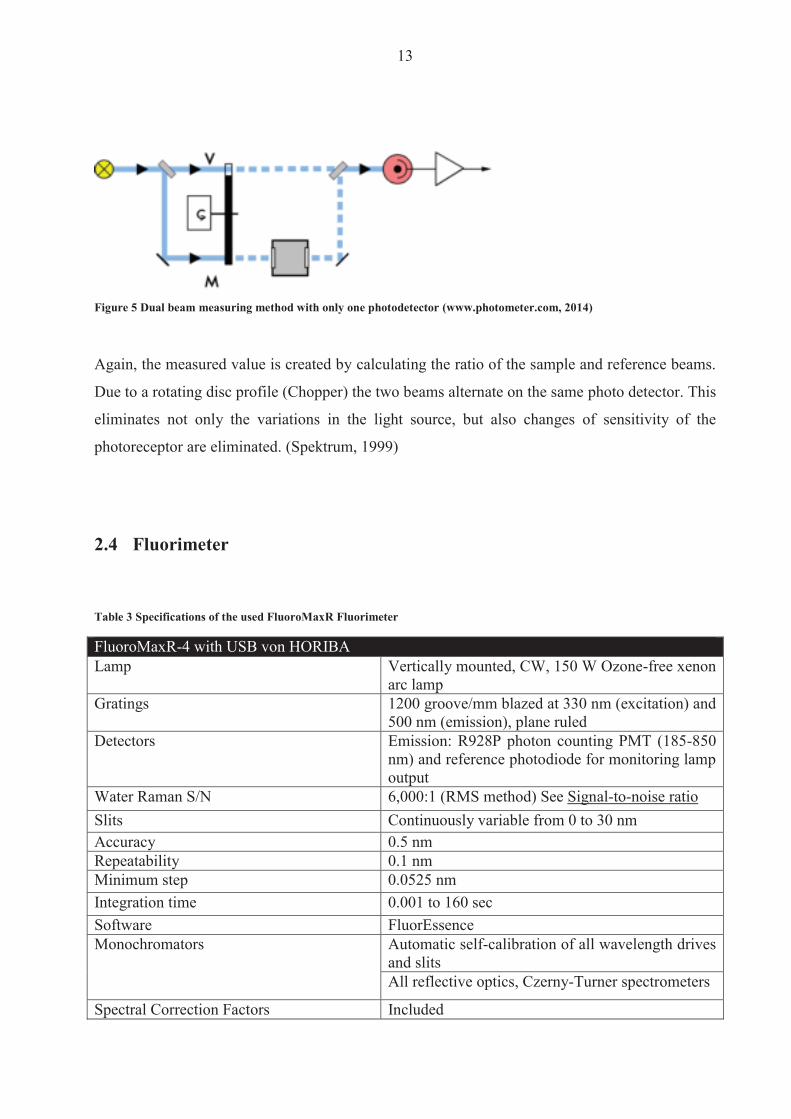
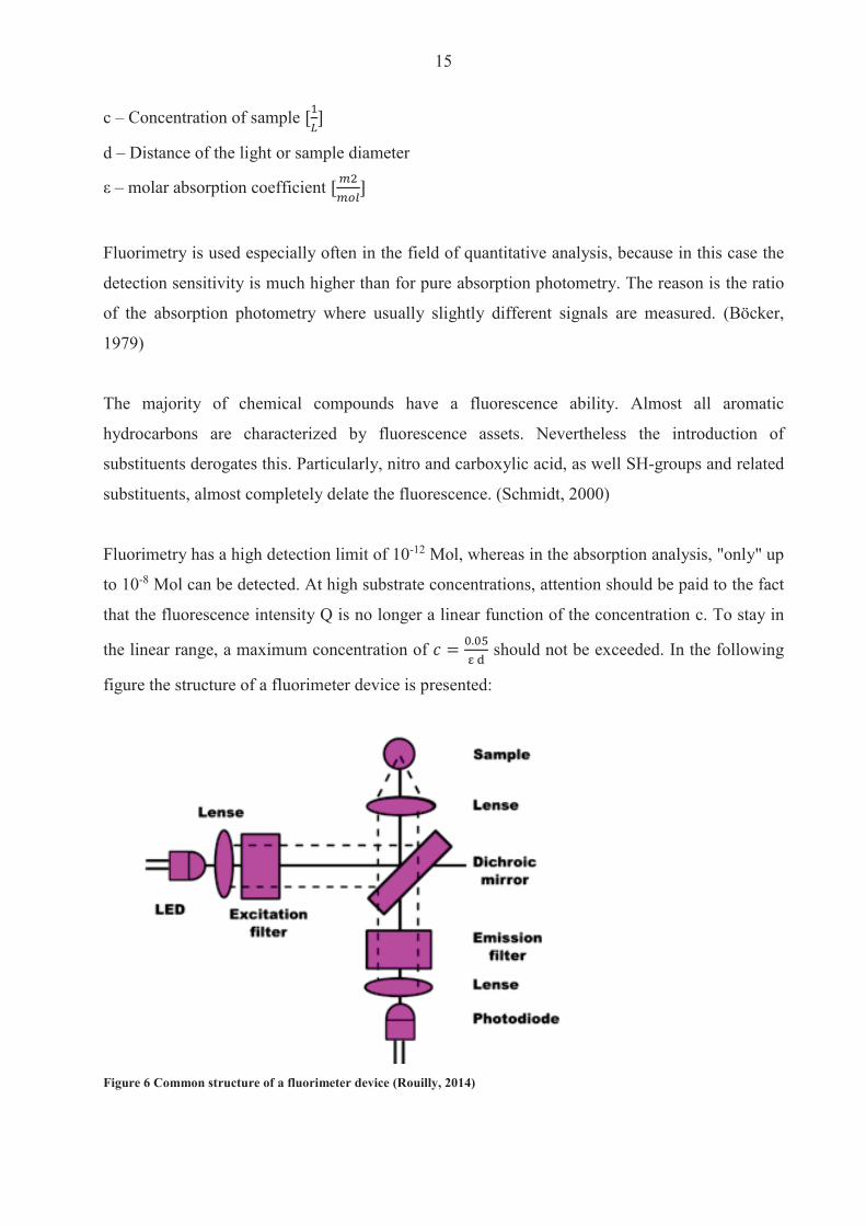
15
c ndash Concentration of sample
d ndash Distance of the light or sample diameter
ε ndash molar absorption coefficient
Fluorimetry is used especially often in the field of quantitative analysis because in this case the
detection sensitivity is much higher than for pure absorption photometry The reason is the ratio
of the absorption photometry where usually slightly different signals are measured (Boumlcker
1979)
The majority of chemical compounds have a fluorescence ability Almost all aromatic
hydrocarbons are characterized by fluorescence assets Nevertheless the introduction of
substituents derogates this Particularly nitro and carboxylic acid as well SH-groups and related
substituents almost completely delate the fluorescence (Schmidt 2000)
Fluorimetry has a high detection limit of 10-12 Mol whereas in the absorption analysis only up
to 10-8 Mol can be detected At high substrate concentrations attention should be paid to the fact
that the fluorescence intensity Q is no longer a linear function of the concentration c To stay in
the linear range a maximum concentration of should not be exceeded In the following
figure the structure of a fluorimeter device is presented
Figure 6 Common structure of a fluorimeter device (Rouilly 2014)
16
Mercury or xenon lamps are often used as sources of excitation light Mercury vapor lamps emit
a line spectrum with high intensities in the lines (at 254 313 36566 405 546 577 630 nm )
via a low-intensity continuous background Xenon lamps have a continuous emission spectrum
but its intensity decreases in the UV range
Important properties of monochromators are their light intensity the spectral slit width and the
freedom of scattered light In modern appliances imaging holographic gratings are used All
optical elements such as lenses gratings mirrors and beam splitters influenced by their spectral
characteristics influence the intensity and polarization of the reflected and transmitted radiation
as a function of wavelength
Photomultiplier are used as which allow due to their high amplification (106 to 108) the
measuring of lower light intensities up to single photons Depending on the material of the
photocathode different types of photoreceptors can vary in terms of their absolute and spectral
sensitivities The gain of the photomultiplier depends on the applied voltage (Zander 1981)
25 Prototype
The instrument which was used for this project was designed to measure and analyze samples of
microalgae by using the method of a fluorimeter In line with the idea of inexpensive production
the construction is relatively basic A schematic diagram is presented in the graphic below
Figure 7 schematic diagram of the prototype sensor (left) and photo (right) (Rolim Heinen amp Huff 2014)
17
As is shown above the installation is similar to the fluorimeter (qv figure 6) The main
components are an LED light source which sends a light beam into an opaque chamber where
the sample is placed and two optical receptors which are positioned at angles of 180deg and 90deg
In contrast to the fluorimeter only one filter is used here (in the fluorimeter three mochrometers
were used) The filter works in the same manner as the monochrometer and blocks all unwanted
wavelengths so that just one specific or particular spectrum can pass through
Figure 8 Filter ldquoStrawrdquo to eliminate unwished wave length
The filter absorbs undesired wavelengths between 300 and 400 nm but has a transmission of 88
in case of the important spectrum (lt 400 nm) which is not optimal but a calculable factor
since itrsquos the same loss in any sample and series of tests
Even though lasers have excellent characteristics in case of accuracy and wavelength they are
relatively expensive In opposition to LEDs In opposition to LEDs Caused by that an LED light
source is installed together with the two optical sensors The high potency LED lamp emits a
blue light beam which fits well with the potential spectrum of absorbance of the chlorophyll and
should provide optimal requirements for the microalgae
18
26 Measurement of Biomass
The analyses of the biomass provides information about growth rate and as a consequence
thereof biological activity Therefore a vacuum pressure pump was used together with paper
filters with a diameter of 205 μm and a pore size of 14 μm
A sample of 50 ml was taken from the batches and filtered through the paper (weighted before)
while the vacuum pump supported the passaging of the liquid Afterwards the nearly-dry paper
was stored in an oven at 60 degC for approximately 24 hours The mass difference gives some
indication of the amount of biomass in the 50 ml solution
27 Measurement of Chlorophyll
An issue in chlorophyll measurement is extracting the pigments from the cells Therefore a
sample of 10 ml is filtered (same procedure as for biomass) The extract is stored afterwards in a
90 acetone solution at 4 degC for approximately 24 hours Acetone is a moderate polar solvent
which is after methanol the best solution for chlorophyll pigments because it consists of polar
areas as well as a lipophilic phytel rest (see figure 9) (Lourenccedilo 2006)
Figure 9 Chemical structure of chlorophyll (Willows 2013)
19
Due to the reference (Lourenccedilo 2006) the solution should be centrifuged for around 10 minutes
and 3000 rpm This strategy is used because usually the filter is cut in pieces before stored in the
tube to guarantee a better detachment of the chlorophyll The pre-tests have shown that the
results are more accurate when the filter isnrsquot cut but rolled up and put into the tube (filtrate
towards the tubes inside) If than filled carefully up with acetone (washing out of the extract
must be avoided during infusion) the extraction of chlorophyll will be optimal without the
problem of filter rests and other cell bodies
In a further step the chlorophyllacetone solution is measured in a spectrophotometer by 630 nm
647 nm and 663 - 665 nm The amount of chlorophyll is calculated by the following statistic
equations from Lourenccedilo (2006)
D663-665 D647 D630 ndash absorbance at the wavelength Dx after correction by the cell-to-cell blank and subtraction of the cell-to-cell blank corrected absorbance at 750nm
l - Cell (cuvette) length [cm] = 1
v - Volume of acetone [ml] = 10
V - Volume of filtered water [l] = 10
Accordingly the term That simplifies the equations
20
3 Results and discussion
During the project the algae suspension was scanned over a time interval of 10 days plus one
day incubation During this time the batches were subjected to various light conditions (Batch A
= 4000 Lux Batch B = 5500 Lux Batch C = 7000 Lux Batch D = 8500 Lux Batch E = 10000
Lux) This was performed to analyze the effect of different light intensity on algae and
accumulation of chlorophyll To obtain useful results it is essential to eliminate as much
unwished problems as possible According to this the growing of the algae was analyzed at first
because any discrepancies of the algae growth would lead to consequential errors in case of
chlorophyll tests
31 Algae growth The growth of Scanedesmus Sp was measured via spectrophotometer and biomass dry weight
Optical density of biomass was determined at 750 nm One ml of the sample batch was taken and
measured in a spectrum between 400 nm and 750 nm
Usually the growth of an algae culture follows certain steps It starts with the lag phase (1)
followed by an exponential phase (2) The culture growth will reach a point of overpopulation in
which one or more essential resources are limited Growth and death rate are either in
equilibrium or the cells already stopped the proliferation This is called the stationary phase (4)
At the end the living conditions are so bad that the cell population starts to decrease rapidly
(usually caused by a deficiency of important nutrients) The last phase is called death phase (5)
Figure 10 Sketch of algae growth dynamics
21
The before explained growth dynamic differs to the culture development during the test Figure 7
(below) presents all graphs (of absorbance [400hellip750 nm]) of the five batches in a time interval
of ten days So in total 50 single graphs summarized in that 3D - graphic It gives an interesting
overview of the total experiment
Figure 11 Progress of all 5 batches in a time interval of 11 days
In the figure a formation can be seen that looks like one side of a steep ridge that starts relatively
flat in the beginning and becomes steeper in the posterior tier Rifts in the formation are caused
by some problems associated with the spectrophotometer at certain wavelengths Following the
observation that the results are the same regardless of the kind of sample analyzed the
assumption that the spectrophotometer doesnrsquot work at these wave length may be accepted
Furthermore a pattern of wave formations is recognizable Every wave formation has a
maximum at around 400 nm and 480 nm and between 650 nm and 670 nm The first ldquowaverdquo is
the result of the batch analyses from the first day the second from the second day and so on
The wavelike formation is caused by the differential growth of the algae under different light
22
conditions The most exposed batch (E) already has a higher algae concentration on dayx as
compared to the lowest exposed batch (A) one day after
Figure 12 By comparison absorbance between 400 nm and 750 nm of five batches at day 6 and 72
The first figure curvebatch E has the highest absorbance starting between 06 and 065 at 400
nm and ending up at the second maximum at around 059 In comparison batchcurve A from
one day after also starts between 06 and 065 but falls under the values of Batch E at the second
maximum which occurs at around 056 This is responsible for the wave effect between the
days Only at the last day does Batch A exceed the high peaks of Batch E from the previous day
This is caused by the beginning of the exponential phase Unfortunately the cultures did not pass
through all four phases as expected The exponential phase started between day 7 and 9
depending on the Batch
2 The days are chosen randomly to proof the above delineated statement The same course of curves could be confirmed for every day Just the intensity of absorbance varies
23
We can see the effect of light between the different figures The culture of Batch E already began
exponential growth at day 7 while the lag phase in Batch A persisted until the 8th9th day
Figure 13 Progress of culture growth comparing Batch E (left) and A (right) during the 10 days in comparison to the Absorbance
The following statements can be made to summarize the observed algae growth Since the
different colonies in the Batches react to the light intensity as expected the assertion can be
made that the Biomass (mB) of
When comparing the results of the optical density with the gravimetric measurements some
issues have to be mentioned The dry weight measurement was only performed after day four
because the amount of biomass measured before day five was considered too small to be reliably
assessed Even after the fifth day some unexpected changes in the curve shape were visible
Nonetheless the main shape of the curve approximates an exponential slope after day eight
which is consistent with the measurement of the optical density
24
Figure 14 Dry weight (mgl) of Scenedesmus Sp for 10 days grown under different light conditions
In addition the amount of biomass increases daily in every Batch according to the results of the
optical density
This is not so in the case of the dry weight measurement where no decipherable pattern can be
determined for the first half of the test period Some problems occurred during the laboratory
processing including the malfunctioning of an oven during day 6 and a restoration of the
samples during day seven Additionally as a consequence of the high error-proneness of the
earlier dry weight analysis due to the use of relatively small volumes findings from the dry
weight analyses should be considered with caution
Beyond these issues it has to be mentioned that the colonies didnrsquot reach the stationary phase
and thus also failed reach the death phase These two statuses of the growth dynamic could
have been interesting for the comparison of the algaechlorophyll ratio while exposed to different
light intensities
25
The results of biomass and spectrophotometer analyses confirm the findings of the designed
prototype in the way that the order of the batches in proportion to dissolved substances (
biomass) is the same as the order of the Batches themselves (BA lt BB lt BC lt BD lt BE dayx)
Figure 15 Algae development measured by prototype during the days 7 - 11 plotted as a function of voltage
The figure above shows the general light intensity that passes through the sample filled with
water (~ 245 V) The larger the amount of dissolved material in the sample the less light will
pass through it and consequently the lower the measured voltage will be With a general
tendency toward a lower voltage a larger amount of biomass can be ascertained but it has to be
mentioned that no statements about the type of curve shape can be made Unfortunately more
test results would have been necessary to make further statements
0
05
1
15
2
25
3
7 8 9 10 11
Outp
ut vo
ltage
at 1
80deg(
V)
Days
A
B
C
D
E
Water
26
32 Chlorophyll formation
After the chlorophyll-acetone mix is stored for 24 hours it is analyzed with a spectrophotometer
For the calculation of chlorophyll content according to Jeffrey amp Humphrey (1975) only some
wavelengths are important Nevertheless the chlorophyll was treated in the same way as the
algae and measurements were made in the range of 400 nm to 750 nm in order to determine
possible similarities
Figure 16 Chlorophyll (mgl) of Scenedesmus sp for 10 days grown under different illumination conditions
The concentration of total chlorophyll increases during the test The results show a steady growth
if expressed as the exponential regression curve (dotted lines) for Batches D and E (R = 09) A
better correlation is shown for a linear regression for Batches A and B (R = 09 instead of 076)
Batch C doesnrsquot show a strong correlation under either a linear (R = 072) or an exponential
growth (R = 076) assumption Many factors affect the results of the Chlorophyll measurement
Firstly the analyses are susceptible to mistakes made during the processing When removing 10
ml from the batches with a concentration of barely 1 mgL and using those samples in a cuvette
of 3 mL the amount of Chlorophyll is typically in a range of 0 ndash 10 μgmL Working with such
small quantities can lead to inaccuracies during processing in addition to errors made on behalf
of the measuring engine itself
Rsup2 = 07602
Rsup2 = 07602
Rsup2 = 09004
Rsup2 = 09037
Rsup2 = 07594
0
05
1
15
2
25
0 1 2 3 4 5 6 7 8 9 10 11
Chlo
roph
yll a
+b (m
gl)
Day
C
D
E
B
A
Expon (C)
Expon (C)
Expon (C)
Expon (D)
Expon (D)
Expon (E)
Linear (B)
Expon (A)
Linear (A)
27
Nevertheless we can make the assumption that the tendency (daily increase) makes sense The
results of the pilot engine show slightly decreasing curves At day 8 there is an obvious mistake
to declare This is not visible with regard to algae measurement at day 93 This leads to the
assumption of a mistake made during the preparing procedure with acetone Since the
abnormality can be found in all batches a mistake during the withdrawal can be ruled out
Figure 17 Chlorophyll development during the days 7 - 11 plotted as a function of voltage
A further problem is that the curves are not clearly separable They cross each other without
showing a decipherable trend with regard to which batch has the highest or the lowest
translucency (which would be proportional to the voltage) As a consequence these results
cannot provide information about the effect of different light irradiation and it is questionable
whether they can be used to make an assumption about chlorophyll accumulation
3 The spectrophotometer analyzes of chlorophyll is one day after due to the 24 hours storing of the samples
0
05
1
15
2
25
3
7 8 9 10 11
Outp
ut vo
ltage
at 1
80deg(
V)
Days
E
B
C
D
A
Water
28
33 Correlation of Algae and Chlorophyll growth The main rationale for using different light irradiation for the Batches was to determine the
relationship between algae growth and the Chlorophyll enhancement Hence interest lay beyond
simply examining the thesis that the concentration of Chlorophyll is directly linked to the algae
growth Furthermore there was interest in exploring whether a specific relationship existed
between the algae growth rate the exposure to light and the amount of chlorophyll produced
Figure 18 Collocation of AlgaeChlorophyll absorbance (by 665 nm) by a spectrophotometer for 11 days
Unfortunately an incomplete test phase (no algae growth until the stationary phase) was
responsible for a lack of results that could be used for further analysis Nevertheless the ratio of
Chlorophyll-to-Algae growth shows a decent progression (see also Table 4) There is no
evidence for a similar progression if the tests proceed for one or two weeks In theory the
chlorophyll concentration should increase more rapidly in the exponential phase (until now the
progress is best described as a linear growth) Furthermore the concentration of algae as well as
of chlorophyll from batch E should reach its maximum first followed by batch D C B A (in
this order) and continue at a stationary rate
BAA
lgae
BAC
hlBB
Alg
aeBB
Chl
BCA
lgae
BCC
hl
BDA
lgae
BDC
hl
BEA
lgae
BEC
hl
002040608
112141618
12
34
56
78
9 1011
BatchSubstrate
Abso
rban
ce
Days
BAAlgae
BAChl
BBAlgae
BBChl
BCAlgae
BCChl
BDAlgae
BDChl
BEAlgae
BEChl
29
Due to the issues described in the earlier chapters the results from analyses on biomass are less
convincing than those arising from the analyses of the spectrophotometer In addition and
contrary to the absorbance measurement the values of dry weight and calculated chlorophyll
correlate weakly in cases of batches with higher light saturation This may be due to inaccuracies
from the dry weight results or another reason could be the earlier start of a kind of exponential
growth for the chlorophyll while the results for the biomass donrsquot show an exponential increase
until the 7th day
Table 4 Overview of the results of biomass prototype and spectrophotometer analyzes
Substrate Biomass (mgl) ndash Dry weight and Chl Optical density (V) -
Prototype Absorbance - Spectrophotometer
Min Max R Min Max R Min Max R BAAlgae 146 327
092 185 061
- 013 156
094 BAChl 001 164 212 170 001 017 BBAlgae 154 444
085 124 049
- 013 169
089 BBChl 004 172 206 175 001 026 BCAlgae 170 478
078 097 042
- 012 170
082 BCChl 002 188 194 181 001 023 BDAlgae 162 504
068 104 044
- 011 172
094 BDChl 002 124 196 171 001 026 BEAlgae 160 515
066 130 035
- 009 175
097 BEChl 002 114 215 195 001 031 The less exciting results are unfortunately given by the Prototype Here no significant correlation
can be mentioned at all In contrast to the spectrophotometer these values are provided by the
direct transmission Therefore the highest solution has the lowest value because more light is
absorbed by the dissolved material which is in this case biomass (or pure chlorophyll) This
result is surprisingly disappointing because the tests performed beforehand with fluorescence
(realized by Leonardo M Rolim) show a straight dependency of proportional relationship
between percental solution and transmission (see Figure 19 below)
Fluorescein is a fluorescent dye from the group of the xanthene It was used for the previous tests
because itrsquos a non-biological and well known substance with which all unwished side effects of a
living system can be avoided during tests
30
Figure 19 Measuring points of concentration given in optical density from fluorescence (Rolim Heinen amp Huff 2014)
The graph shows the transmission by 180 degC as accomplished with the algae and chlorophyll
during this work The curve suggests a negative exponential trend This was also expected for the
new series of tests While a clear difference can be recorded in the case of fluorescein the values
of chlorophyll almost didnrsquot change This could be an effect of the high fluorescent impact of
fluorescence Due to the growth rate of chlorophyll (see Table 4 Chl Min and Max) which goes
from 001 gmL up to almost 18 gmL (180 times more) compared with the fluorescence which
goes from 001 gmL up to 03 gmL (30 times more) this is questionable since the concentration
difference is 5 times higher for pure chlorophyll a fluorescent pigment as well but the effect is
very little Nevertheless it could be an indication as to why results from the test were not as
expected
The analyses by the fluorimeter provides further interesting results The figure below presents
the results of chlorophyll for the 11th day The x-axis shows the input of the wave length
produced by the laser The excitation is visible on the y-axis while curves on the graph present
one specific wave length each between 400 and 800 nm (with an interval of 5 ie a new
measurement was performed for every 5 nm) In order to simplify the graphical presentation the
legend was omitted
31
Figure 20 Display of emission and excitation measured by the fluorimeter of day 11 for chlorophyll
The figure provides an important insight into the behavior of chlorophyll fluorescent The
formation on the bluish part of the light spectrum (270 ndash 430 nm) and the second cluster of peaks
between 650 and 675 nm are quite revealing The table below explains the most important
curves
Table 5 Legend of figure 16
Color wave length (nm) red 675 blue 670 gray 680
light green 665 orange 685
light blue 660 dark blue 690 dark green 695
These eight curves are explicitly mentioned because they have the highest response in the tested
emission spectrum Due to usually low concentrations of samples eg chlorophyll in μgml a
high response is vital The results of the other test days are equal They simply vary in the height
of excitation as a result of a higher concentration
0
200000
400000
600000
800000
1000000
1200000
1400000
1600000
300 325 350 375 400 425 450 475 500 525 550 575 600 625 650 675 700 725 750
Exita
tion
ampe
rage
at 9
0deg(m
A)
Emission wave lenght (nm)
32
Figure 21 Display of emission and excitation measured by the fluorimeter between the days 0 and 11 for chlorophyll (BA)
The daily difference of the excitation is presented above The course of the curves is equal and
just differs as mentioned before in the amount of ampere measured by the receptor The same
shape would be plotted by the other batches The only difference again would be the level of
excitation
The progression of the chlorophyll curves during the tests shows a permanent increase beginning
at day three An exponential correlation can be verified for the plotted curves Thus the results
from the fluorimeter are as expected before Still the problem as mentioned before of the
incomplete growth of the algae was responsible for a lack of further information which could
have been interesting
0
200000
400000
600000
800000
1000000
1200000
350 375 400 425 450 475 500 525 550 575 600 625 650 675 700 725 750
Excit
atio
n am
pera
ge a
t 90
deg(m
A)
Emission wave lenght (nm)
0
1
2
3
4
5
6
7
8
9
10
11
33
Figure 22 Trend of the chlorophyll excitation peaks during 11 days measured by the fluorimeter
In the following section the results from the algae analyses are explained One problem has to be
mentioned beforehand
The graph below shows the outcome from the last day Highly overlapping curves are visible
This is not caused by fluorescence but by the reflection of each wave length itself due to a high
solution The analyses made by the fluorimeter requires at least 30 minutes That it enough time
for the dissolved particle to settle down The x-axis can accordingly be viewed as a timeline
scale As more time passes by the reflection impact reduces
Rsup2 = 08453
0
200000
400000
600000
800000
1000000
1200000
1400000
1600000
1800000
2000000
0 2 4 6 8 10 12
Excit
atio
n am
pera
ge a
t 90
deg(m
A)
Days
660
665
430
405
375
Log (375)
34
Figure 23 Fluorimeter results of algae (BA day11)4
When the y-axis is limited to 100000 mA some other formations are visible Interestingly they
have the same shape as the curves of the chlorophyll which leads to the assumption that those
overlapped curves are indeed the fluorescent impact of the chlorophyll pigments
4 Every curve presents one wave length of the emission spectrum in an interval of five The legend is once more excluded due to a better overview
0
1000000
2000000
3000000
4000000
5000000
6000000
7000000
8000000
300 325 350 375 400 425 450 475 500 525 550 575 600 625 650 675 700 725 750
Excit
atio
n am
pera
ge a
t 90deg
(mA)
Emission wave lenght (nm)
35
Figure 24 Fluorimeter results of algae (BA day11) with limited y-axes up to 100000 mA5
On closer examination it can be interpreted that the higher curves (blue orange green dark
blue redhellip) are the same wavelengths as seen in the Table 5 Legend of figure 16rdquo The highest
response again is at 675 nm Measureing by a different wave length than 675 nm will cause
lower excitation The same happens in case of chlorophyll
The excitation is low in comparison with the results of the pure chlorophyll because the
chlorophyll is not separated from the cells which hinders the light from reaching the pigments
in addition to leaving the sample and stimulating the receptor
The comparison with the other batches and the analyses of the different days provides the same
results as for the chlorophyll That means the Excitation of BA(dx) lt BB(dx) lt BC(dx) lt BD(dx)
lt BE(dx) and the Excitation of BA(dx) lt BA(dx+1) BB(dx) lt BB(dx+1) BC(dx) lt BC(dx+1)
BD(dx) lt BD(dx+1) BE(dx) lt BE(dx+1)
5 The legend is once more excluded due to a better overview
0
10000
20000
30000
40000
50000
60000
70000
80000
90000
100000
300 325 350 375 400 425 450 475 500 525 550 575 600 625 650 675 700 725 750
Excit
atio
n am
pera
ge a
t 90
deg(m
A)
Emission wave lenght (nm)
36
4 Conclusiones
According to the results from the fluorimeter the algae growth and chlorophyll enhancement
appear to be as expected This leads to the question as to why the previous tests donrsquot have
similar outcomes The answer to this question and the reason why fluorimeters are used for low
quantities is the same They have a very high accuracy and are thus extremely efficient even
for low quantities Nevertheless they are extremely expensive and the main task of this project
was to determine whether it was possible to measure chlorophyll (pure or even intracellular) with
the prototype or if not to work out further steps for the development of the engine
The first step apart from the biological section is to make the engine more stable During the
project problems often occurred with regard to replication of results because small changes in the
electrical connection contributed to different outcomes while using the same sample This made
the testing more complicated and made unnecessary repetitions of measurement indispensable A
shell for the entire construction in which the electronic is fixed should solve this problem An
extension cable which leads to the measuring box together with a smaller diameter of the cell
itself would also be useful The laser and the two receptors should be installed separately from
the cell and waterproofed (plastic and glue should be sufficient) As a result the cell could be
introduced into a sample to measure which not only simplifies the procedure but it is also closer
to any practical application
The next action is the acquisition of the correct optical filter The results of the fluorimeter
suggest an optimal emission at 430 plusmn 10 nm while the excitation should be measured at 675 plusmn 10
nm The closer the measurement is to these wavelengths the higher the values of the results
Furthermore it was explained how other wave lengths overlap the fluorescence effect This can
be avoided by use of at least two filters one which filters the light of the laser and blocks out
every wavelength except for those in the range of eg 420 ndash 440 nm and a second filter which
allows for only the spectrum from 665 to 685 nm to pass
Nevertheless an upgrade of either the receptor or laser but probably both will be inevitable As
mentioned in the previous chapter the outcome of the 90deg measurement for algae and
chlorophyll is almost zero In actuality it has the same value as if measured with water which
means that the receptor is not able to recognize any approaching light On the other hand it may
37
be that the laser is too weak so that not enough light is injected In any case adjustment for the
right filter range should be the first step
When the filter and laserreceptor problems are solved a new test with fluorescence would make
sense At this stage it is important not only that the results are good for one series of tests but
also that they are repeatable Daily calibration of the engine is not only effortful and time-
consuming but it can also lead to variable results After good and stable results are achieved
with fluoresce a new test series with algae can be started Therefore it would be useful to create
a serial dilution of an algae culture which is already in the stationary phase and highly
concentrated If the results are suitable it can be continued with a serial dilution of those algae
Even if the results from the 90deg measurement are not satisfying a further test with pure
chlorophyll could be accomplished on condition that the results from the 180deg measurement are
decent
Only after all the described experiments have sufficient results should a new long-term test series
be started For this purpose no more than three batches should be installed with an intensity of
illumination between 3000 and 10000 lux The test duration should be approximately 30 days to
ensure that the culture passes through all growing and dying phases Tests performed with the
spectrophotometer can indicate a change of the growing conditions so that further and more
elaborated tests with the fluorimeter and biomass can be performed The measurement of
biomass should be sufficient if performed every three days (a daily testing during the exponential
phase would perhaps be useful) By using the fluorimeter care has to be taken so that the dilution
of the sample is large enough otherwise overlapping effects occur The analyses with the sensor
should be performed daily in order to get a consistent overview of the chlorophyllalgae ratio as
well as to gauge the accuracy of the sensor
38
5 Bibliography Boumlcker J (1979) Spektroskopie Instrumentelle Analytik mit Atom- und Molekuumllspektroskopie
(1 Edition Ausg) Wuumlrzburg Vogel Verlag und Druck GmbH amp Co
Hegewald P (2006) Scenedesmusndashlike algae of Ukraine Tsarenko E amp B Braband
Lehmann E W (1892) Uumlber ein Photometer Erlangen
Lourenccedilo S (2006) Cultivo de Microalgas Marinhas Princiacutepios e Aplicaccedilotildees
Luumlrling M (1999) The Smell of Water Grazer-Induced Colony Formation in Scenedesmus
Wageningen Pulz und Gross
Mills I Cvitaš T Homann K Kallay N amp Kuchitsu K (1993) Quantities Units and
Symbols in Physical Chemistry (Green Book)
Rolim L M Heinen A L amp Huff D D (2014) Desenvolvimento de sensor oacuteptico portaacutetil
para mediccedilatildeoes online de concentraccedilatildeo no cultivo de microalgas Porto Alegre
Rouilly V (2014) Schmidt W (2000) Optische Spektroskopie (Bd 2 Edition) Weinheim
WILEY-VCH Verlag GmbH
Unknown (1999) Photometer Spektrum Akademischer Verlag
Willows R D (2013) Structure of chlorophyll Organic Letters
Zander M (1981) Fluorimetrie Berlin-Heidelberg-New York Springer-Verlag
Internet sources Openwetwareorg
photometercom
teachingshuacuk
wikipediaorg
39
6 List of figures Figure 1 Pilot batch deployment 7
Figure 2 Relation between transmittance and absorbance 9
Figure 3 Structure of a photometer 10
Figure 4 Structure of a photometer with a dual-bean 12
Figure 5 Dual beam measuring method with only one photodetector 13
Figure 6 Common structure of a fluorimeter device 15
Figure 7 schematic diagram of the prototype sensor (left) and photo (right) 16
Figure 8 Filter ldquoStrawrdquo to eliminate unwished wave length 17
Figure 9 Chemical structure of chlorophyll 18
Figure 10 Sketch of algae growth dynamics 20
Figure 11 Progress of all 5 batches in a time interval of 11 days 21
Figure 13 By comparison absorbance between 400 nm and 750 nm of five batches at day 6 and 7
22
Figure 14 Progress of culture growth comparing Batch E (left) and A (right) during the 10 days
in comparison to the Absorbance 23
Figure 15 Dry weight (mgl) of Scenedesmus Sp for 10 days grown under different light
conditions 24
Figure 16 Algae development measured by prototype during the days 7 - 11 plotted as a function
of voltage 25
Figure 17 Chlorophyll (mgl) of Scenedesmus sp for 10 days grown under different illumination
conditions 26
Figure 18 Chlorophyll development during the days 7 - 11 plotted as a function of voltage 27
Figure 19 Collocation of AlgaeChlorophyll absorbance (by 665 nm) by a spectrophotometer for
11 days 28
Figure 20 Measuring points of concentration given in optical density from fluorescence 30
Figure 21 Display of emission and excitation measured by the fluorimeter of day 11 for
chlorophyll 31
Figure 22 Display of emission and excitation measured by the fluorimeter between the days 0
and 11 for chlorophyll (BA) 32
Figure 23 Trend of the chlorophyll excitation peaks during 11 days measured by the fluorimeter
33
Figure 24 Fluorimeter results of algae (BA day11) 34
Figure 25 Fluorimeter results of algae (BA day11) with limited y-axes up to 100000 mA 35
40
7 List of tables Table 1 Composition of algae supplementary medium 6
Table 2 Specifications of the used T80 spectrophotometer 11
Table 3 Specifications of the used FluoroMaxR Fluorimeter 13
Table 4 Overview of the results of biomass prototype and spectrophotometer analyzes 29
Table 5 Legend of figure 16 31
41
Declaration of Authorship I hereby certify that this work has been composed by me and is based on my own work
unless stated otherwise No other person`s work has been used without due
acknowledgement in this report All references and verbatim extracts have been quoted
and all sources of information including graphs and data sets have been specifically
acknowledged
______________________ ________________________ Ort Datum Signature
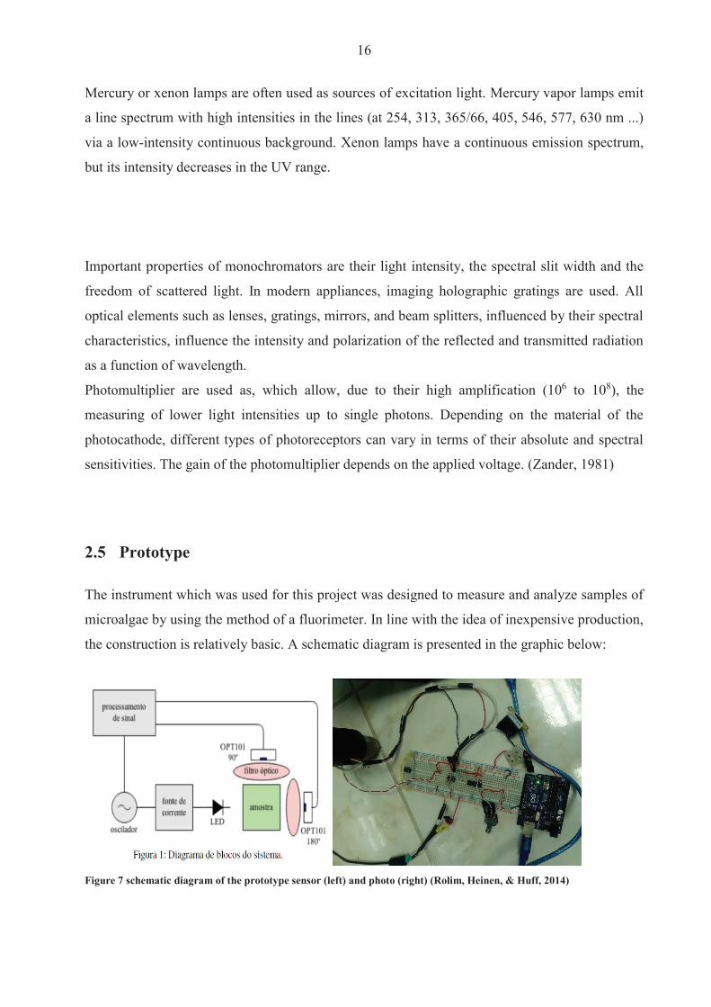
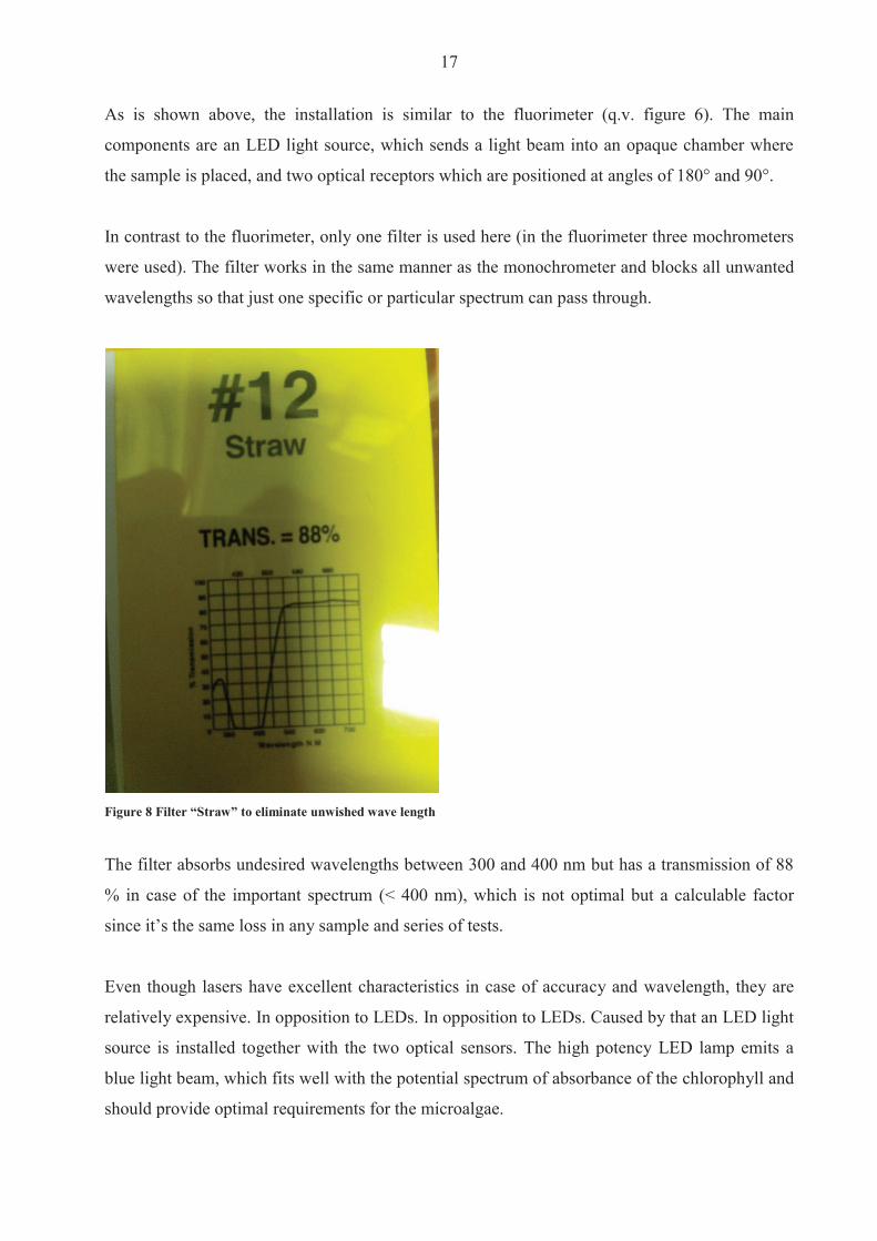
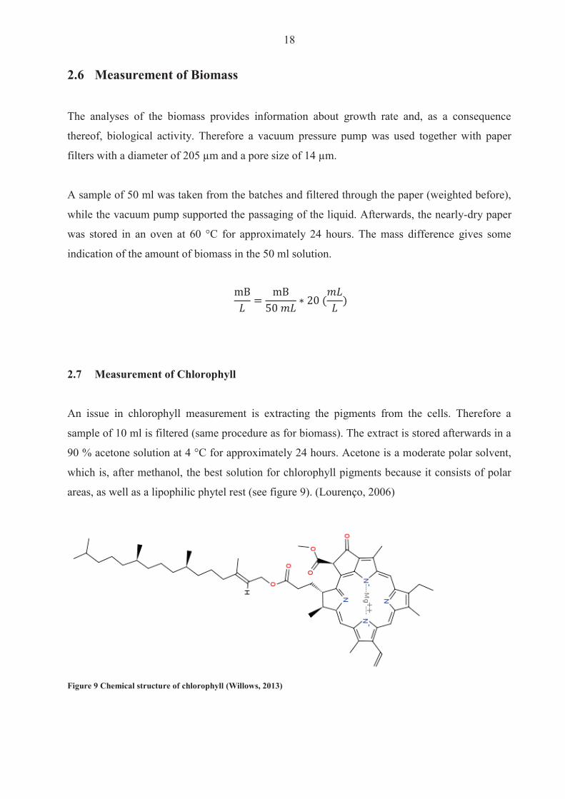

22
conditions The most exposed batch (E) already has a higher algae concentration on dayx as
compared to the lowest exposed batch (A) one day after
Figure 12 By comparison absorbance between 400 nm and 750 nm of five batches at day 6 and 72
The first figure curvebatch E has the highest absorbance starting between 06 and 065 at 400
nm and ending up at the second maximum at around 059 In comparison batchcurve A from
one day after also starts between 06 and 065 but falls under the values of Batch E at the second
maximum which occurs at around 056 This is responsible for the wave effect between the
days Only at the last day does Batch A exceed the high peaks of Batch E from the previous day
This is caused by the beginning of the exponential phase Unfortunately the cultures did not pass
through all four phases as expected The exponential phase started between day 7 and 9
depending on the Batch
2 The days are chosen randomly to proof the above delineated statement The same course of curves could be confirmed for every day Just the intensity of absorbance varies
23
We can see the effect of light between the different figures The culture of Batch E already began
exponential growth at day 7 while the lag phase in Batch A persisted until the 8th9th day
Figure 13 Progress of culture growth comparing Batch E (left) and A (right) during the 10 days in comparison to the Absorbance
The following statements can be made to summarize the observed algae growth Since the
different colonies in the Batches react to the light intensity as expected the assertion can be
made that the Biomass (mB) of
When comparing the results of the optical density with the gravimetric measurements some
issues have to be mentioned The dry weight measurement was only performed after day four
because the amount of biomass measured before day five was considered too small to be reliably
assessed Even after the fifth day some unexpected changes in the curve shape were visible
Nonetheless the main shape of the curve approximates an exponential slope after day eight
which is consistent with the measurement of the optical density
24
Figure 14 Dry weight (mgl) of Scenedesmus Sp for 10 days grown under different light conditions
In addition the amount of biomass increases daily in every Batch according to the results of the
optical density
This is not so in the case of the dry weight measurement where no decipherable pattern can be
determined for the first half of the test period Some problems occurred during the laboratory
processing including the malfunctioning of an oven during day 6 and a restoration of the
samples during day seven Additionally as a consequence of the high error-proneness of the
earlier dry weight analysis due to the use of relatively small volumes findings from the dry
weight analyses should be considered with caution
Beyond these issues it has to be mentioned that the colonies didnrsquot reach the stationary phase
and thus also failed reach the death phase These two statuses of the growth dynamic could
have been interesting for the comparison of the algaechlorophyll ratio while exposed to different
light intensities
25
The results of biomass and spectrophotometer analyses confirm the findings of the designed
prototype in the way that the order of the batches in proportion to dissolved substances (
biomass) is the same as the order of the Batches themselves (BA lt BB lt BC lt BD lt BE dayx)
Figure 15 Algae development measured by prototype during the days 7 - 11 plotted as a function of voltage
The figure above shows the general light intensity that passes through the sample filled with
water (~ 245 V) The larger the amount of dissolved material in the sample the less light will
pass through it and consequently the lower the measured voltage will be With a general
tendency toward a lower voltage a larger amount of biomass can be ascertained but it has to be
mentioned that no statements about the type of curve shape can be made Unfortunately more
test results would have been necessary to make further statements
0
05
1
15
2
25
3
7 8 9 10 11
Outp
ut vo
ltage
at 1
80deg(
V)
Days
A
B
C
D
E
Water
26
32 Chlorophyll formation
After the chlorophyll-acetone mix is stored for 24 hours it is analyzed with a spectrophotometer
For the calculation of chlorophyll content according to Jeffrey amp Humphrey (1975) only some
wavelengths are important Nevertheless the chlorophyll was treated in the same way as the
algae and measurements were made in the range of 400 nm to 750 nm in order to determine
possible similarities
Figure 16 Chlorophyll (mgl) of Scenedesmus sp for 10 days grown under different illumination conditions
The concentration of total chlorophyll increases during the test The results show a steady growth
if expressed as the exponential regression curve (dotted lines) for Batches D and E (R = 09) A
better correlation is shown for a linear regression for Batches A and B (R = 09 instead of 076)
Batch C doesnrsquot show a strong correlation under either a linear (R = 072) or an exponential
growth (R = 076) assumption Many factors affect the results of the Chlorophyll measurement
Firstly the analyses are susceptible to mistakes made during the processing When removing 10
ml from the batches with a concentration of barely 1 mgL and using those samples in a cuvette
of 3 mL the amount of Chlorophyll is typically in a range of 0 ndash 10 μgmL Working with such
small quantities can lead to inaccuracies during processing in addition to errors made on behalf
of the measuring engine itself
Rsup2 = 07602
Rsup2 = 07602
Rsup2 = 09004
Rsup2 = 09037
Rsup2 = 07594
0
05
1
15
2
25
0 1 2 3 4 5 6 7 8 9 10 11
Chlo
roph
yll a
+b (m
gl)
Day
C
D
E
B
A
Expon (C)
Expon (C)
Expon (C)
Expon (D)
Expon (D)
Expon (E)
Linear (B)
Expon (A)
Linear (A)
27
Nevertheless we can make the assumption that the tendency (daily increase) makes sense The
results of the pilot engine show slightly decreasing curves At day 8 there is an obvious mistake
to declare This is not visible with regard to algae measurement at day 93 This leads to the
assumption of a mistake made during the preparing procedure with acetone Since the
abnormality can be found in all batches a mistake during the withdrawal can be ruled out
Figure 17 Chlorophyll development during the days 7 - 11 plotted as a function of voltage
A further problem is that the curves are not clearly separable They cross each other without
showing a decipherable trend with regard to which batch has the highest or the lowest
translucency (which would be proportional to the voltage) As a consequence these results
cannot provide information about the effect of different light irradiation and it is questionable
whether they can be used to make an assumption about chlorophyll accumulation
3 The spectrophotometer analyzes of chlorophyll is one day after due to the 24 hours storing of the samples
0
05
1
15
2
25
3
7 8 9 10 11
Outp
ut vo
ltage
at 1
80deg(
V)
Days
E
B
C
D
A
Water
28
33 Correlation of Algae and Chlorophyll growth The main rationale for using different light irradiation for the Batches was to determine the
relationship between algae growth and the Chlorophyll enhancement Hence interest lay beyond
simply examining the thesis that the concentration of Chlorophyll is directly linked to the algae
growth Furthermore there was interest in exploring whether a specific relationship existed
between the algae growth rate the exposure to light and the amount of chlorophyll produced
Figure 18 Collocation of AlgaeChlorophyll absorbance (by 665 nm) by a spectrophotometer for 11 days
Unfortunately an incomplete test phase (no algae growth until the stationary phase) was
responsible for a lack of results that could be used for further analysis Nevertheless the ratio of
Chlorophyll-to-Algae growth shows a decent progression (see also Table 4) There is no
evidence for a similar progression if the tests proceed for one or two weeks In theory the
chlorophyll concentration should increase more rapidly in the exponential phase (until now the
progress is best described as a linear growth) Furthermore the concentration of algae as well as
of chlorophyll from batch E should reach its maximum first followed by batch D C B A (in
this order) and continue at a stationary rate
BAA
lgae
BAC
hlBB
Alg
aeBB
Chl
BCA
lgae
BCC
hl
BDA
lgae
BDC
hl
BEA
lgae
BEC
hl
002040608
112141618
12
34
56
78
9 1011
BatchSubstrate
Abso
rban
ce
Days
BAAlgae
BAChl
BBAlgae
BBChl
BCAlgae
BCChl
BDAlgae
BDChl
BEAlgae
BEChl
29
Due to the issues described in the earlier chapters the results from analyses on biomass are less
convincing than those arising from the analyses of the spectrophotometer In addition and
contrary to the absorbance measurement the values of dry weight and calculated chlorophyll
correlate weakly in cases of batches with higher light saturation This may be due to inaccuracies
from the dry weight results or another reason could be the earlier start of a kind of exponential
growth for the chlorophyll while the results for the biomass donrsquot show an exponential increase
until the 7th day
Table 4 Overview of the results of biomass prototype and spectrophotometer analyzes
Substrate Biomass (mgl) ndash Dry weight and Chl Optical density (V) -
Prototype Absorbance - Spectrophotometer
Min Max R Min Max R Min Max R BAAlgae 146 327
092 185 061
- 013 156
094 BAChl 001 164 212 170 001 017 BBAlgae 154 444
085 124 049
- 013 169
089 BBChl 004 172 206 175 001 026 BCAlgae 170 478
078 097 042
- 012 170
082 BCChl 002 188 194 181 001 023 BDAlgae 162 504
068 104 044
- 011 172
094 BDChl 002 124 196 171 001 026 BEAlgae 160 515
066 130 035
- 009 175
097 BEChl 002 114 215 195 001 031 The less exciting results are unfortunately given by the Prototype Here no significant correlation
can be mentioned at all In contrast to the spectrophotometer these values are provided by the
direct transmission Therefore the highest solution has the lowest value because more light is
absorbed by the dissolved material which is in this case biomass (or pure chlorophyll) This
result is surprisingly disappointing because the tests performed beforehand with fluorescence
(realized by Leonardo M Rolim) show a straight dependency of proportional relationship
between percental solution and transmission (see Figure 19 below)
Fluorescein is a fluorescent dye from the group of the xanthene It was used for the previous tests
because itrsquos a non-biological and well known substance with which all unwished side effects of a
living system can be avoided during tests
30
Figure 19 Measuring points of concentration given in optical density from fluorescence (Rolim Heinen amp Huff 2014)
The graph shows the transmission by 180 degC as accomplished with the algae and chlorophyll
during this work The curve suggests a negative exponential trend This was also expected for the
new series of tests While a clear difference can be recorded in the case of fluorescein the values
of chlorophyll almost didnrsquot change This could be an effect of the high fluorescent impact of
fluorescence Due to the growth rate of chlorophyll (see Table 4 Chl Min and Max) which goes
from 001 gmL up to almost 18 gmL (180 times more) compared with the fluorescence which
goes from 001 gmL up to 03 gmL (30 times more) this is questionable since the concentration
difference is 5 times higher for pure chlorophyll a fluorescent pigment as well but the effect is
very little Nevertheless it could be an indication as to why results from the test were not as
expected
The analyses by the fluorimeter provides further interesting results The figure below presents
the results of chlorophyll for the 11th day The x-axis shows the input of the wave length
produced by the laser The excitation is visible on the y-axis while curves on the graph present
one specific wave length each between 400 and 800 nm (with an interval of 5 ie a new
measurement was performed for every 5 nm) In order to simplify the graphical presentation the
legend was omitted
31
Figure 20 Display of emission and excitation measured by the fluorimeter of day 11 for chlorophyll
The figure provides an important insight into the behavior of chlorophyll fluorescent The
formation on the bluish part of the light spectrum (270 ndash 430 nm) and the second cluster of peaks
between 650 and 675 nm are quite revealing The table below explains the most important
curves
Table 5 Legend of figure 16
Color wave length (nm) red 675 blue 670 gray 680
light green 665 orange 685
light blue 660 dark blue 690 dark green 695
These eight curves are explicitly mentioned because they have the highest response in the tested
emission spectrum Due to usually low concentrations of samples eg chlorophyll in μgml a
high response is vital The results of the other test days are equal They simply vary in the height
of excitation as a result of a higher concentration
0
200000
400000
600000
800000
1000000
1200000
1400000
1600000
300 325 350 375 400 425 450 475 500 525 550 575 600 625 650 675 700 725 750
Exita
tion
ampe
rage
at 9
0deg(m
A)
Emission wave lenght (nm)
32
Figure 21 Display of emission and excitation measured by the fluorimeter between the days 0 and 11 for chlorophyll (BA)
The daily difference of the excitation is presented above The course of the curves is equal and
just differs as mentioned before in the amount of ampere measured by the receptor The same
shape would be plotted by the other batches The only difference again would be the level of
excitation
The progression of the chlorophyll curves during the tests shows a permanent increase beginning
at day three An exponential correlation can be verified for the plotted curves Thus the results
from the fluorimeter are as expected before Still the problem as mentioned before of the
incomplete growth of the algae was responsible for a lack of further information which could
have been interesting
0
200000
400000
600000
800000
1000000
1200000
350 375 400 425 450 475 500 525 550 575 600 625 650 675 700 725 750
Excit
atio
n am
pera
ge a
t 90
deg(m
A)
Emission wave lenght (nm)
0
1
2
3
4
5
6
7
8
9
10
11
33
Figure 22 Trend of the chlorophyll excitation peaks during 11 days measured by the fluorimeter
In the following section the results from the algae analyses are explained One problem has to be
mentioned beforehand
The graph below shows the outcome from the last day Highly overlapping curves are visible
This is not caused by fluorescence but by the reflection of each wave length itself due to a high
solution The analyses made by the fluorimeter requires at least 30 minutes That it enough time
for the dissolved particle to settle down The x-axis can accordingly be viewed as a timeline
scale As more time passes by the reflection impact reduces
Rsup2 = 08453
0
200000
400000
600000
800000
1000000
1200000
1400000
1600000
1800000
2000000
0 2 4 6 8 10 12
Excit
atio
n am
pera
ge a
t 90
deg(m
A)
Days
660
665
430
405
375
Log (375)
34
Figure 23 Fluorimeter results of algae (BA day11)4
When the y-axis is limited to 100000 mA some other formations are visible Interestingly they
have the same shape as the curves of the chlorophyll which leads to the assumption that those
overlapped curves are indeed the fluorescent impact of the chlorophyll pigments
4 Every curve presents one wave length of the emission spectrum in an interval of five The legend is once more excluded due to a better overview
0
1000000
2000000
3000000
4000000
5000000
6000000
7000000
8000000
300 325 350 375 400 425 450 475 500 525 550 575 600 625 650 675 700 725 750
Excit
atio
n am
pera
ge a
t 90deg
(mA)
Emission wave lenght (nm)
35
Figure 24 Fluorimeter results of algae (BA day11) with limited y-axes up to 100000 mA5
On closer examination it can be interpreted that the higher curves (blue orange green dark
blue redhellip) are the same wavelengths as seen in the Table 5 Legend of figure 16rdquo The highest
response again is at 675 nm Measureing by a different wave length than 675 nm will cause
lower excitation The same happens in case of chlorophyll
The excitation is low in comparison with the results of the pure chlorophyll because the
chlorophyll is not separated from the cells which hinders the light from reaching the pigments
in addition to leaving the sample and stimulating the receptor
The comparison with the other batches and the analyses of the different days provides the same
results as for the chlorophyll That means the Excitation of BA(dx) lt BB(dx) lt BC(dx) lt BD(dx)
lt BE(dx) and the Excitation of BA(dx) lt BA(dx+1) BB(dx) lt BB(dx+1) BC(dx) lt BC(dx+1)
BD(dx) lt BD(dx+1) BE(dx) lt BE(dx+1)
5 The legend is once more excluded due to a better overview
0
10000
20000
30000
40000
50000
60000
70000
80000
90000
100000
300 325 350 375 400 425 450 475 500 525 550 575 600 625 650 675 700 725 750
Excit
atio
n am
pera
ge a
t 90
deg(m
A)
Emission wave lenght (nm)
36
4 Conclusiones
According to the results from the fluorimeter the algae growth and chlorophyll enhancement
appear to be as expected This leads to the question as to why the previous tests donrsquot have
similar outcomes The answer to this question and the reason why fluorimeters are used for low
quantities is the same They have a very high accuracy and are thus extremely efficient even
for low quantities Nevertheless they are extremely expensive and the main task of this project
was to determine whether it was possible to measure chlorophyll (pure or even intracellular) with
the prototype or if not to work out further steps for the development of the engine
The first step apart from the biological section is to make the engine more stable During the
project problems often occurred with regard to replication of results because small changes in the
electrical connection contributed to different outcomes while using the same sample This made
the testing more complicated and made unnecessary repetitions of measurement indispensable A
shell for the entire construction in which the electronic is fixed should solve this problem An
extension cable which leads to the measuring box together with a smaller diameter of the cell
itself would also be useful The laser and the two receptors should be installed separately from
the cell and waterproofed (plastic and glue should be sufficient) As a result the cell could be
introduced into a sample to measure which not only simplifies the procedure but it is also closer
to any practical application
The next action is the acquisition of the correct optical filter The results of the fluorimeter
suggest an optimal emission at 430 plusmn 10 nm while the excitation should be measured at 675 plusmn 10
nm The closer the measurement is to these wavelengths the higher the values of the results
Furthermore it was explained how other wave lengths overlap the fluorescence effect This can
be avoided by use of at least two filters one which filters the light of the laser and blocks out
every wavelength except for those in the range of eg 420 ndash 440 nm and a second filter which
allows for only the spectrum from 665 to 685 nm to pass
Nevertheless an upgrade of either the receptor or laser but probably both will be inevitable As
mentioned in the previous chapter the outcome of the 90deg measurement for algae and
chlorophyll is almost zero In actuality it has the same value as if measured with water which
means that the receptor is not able to recognize any approaching light On the other hand it may
37
be that the laser is too weak so that not enough light is injected In any case adjustment for the
right filter range should be the first step
When the filter and laserreceptor problems are solved a new test with fluorescence would make
sense At this stage it is important not only that the results are good for one series of tests but
also that they are repeatable Daily calibration of the engine is not only effortful and time-
consuming but it can also lead to variable results After good and stable results are achieved
with fluoresce a new test series with algae can be started Therefore it would be useful to create
a serial dilution of an algae culture which is already in the stationary phase and highly
concentrated If the results are suitable it can be continued with a serial dilution of those algae
Even if the results from the 90deg measurement are not satisfying a further test with pure
chlorophyll could be accomplished on condition that the results from the 180deg measurement are
decent
Only after all the described experiments have sufficient results should a new long-term test series
be started For this purpose no more than three batches should be installed with an intensity of
illumination between 3000 and 10000 lux The test duration should be approximately 30 days to
ensure that the culture passes through all growing and dying phases Tests performed with the
spectrophotometer can indicate a change of the growing conditions so that further and more
elaborated tests with the fluorimeter and biomass can be performed The measurement of
biomass should be sufficient if performed every three days (a daily testing during the exponential
phase would perhaps be useful) By using the fluorimeter care has to be taken so that the dilution
of the sample is large enough otherwise overlapping effects occur The analyses with the sensor
should be performed daily in order to get a consistent overview of the chlorophyllalgae ratio as
well as to gauge the accuracy of the sensor
38
5 Bibliography Boumlcker J (1979) Spektroskopie Instrumentelle Analytik mit Atom- und Molekuumllspektroskopie
(1 Edition Ausg) Wuumlrzburg Vogel Verlag und Druck GmbH amp Co
Hegewald P (2006) Scenedesmusndashlike algae of Ukraine Tsarenko E amp B Braband
Lehmann E W (1892) Uumlber ein Photometer Erlangen
Lourenccedilo S (2006) Cultivo de Microalgas Marinhas Princiacutepios e Aplicaccedilotildees
Luumlrling M (1999) The Smell of Water Grazer-Induced Colony Formation in Scenedesmus
Wageningen Pulz und Gross
Mills I Cvitaš T Homann K Kallay N amp Kuchitsu K (1993) Quantities Units and
Symbols in Physical Chemistry (Green Book)
Rolim L M Heinen A L amp Huff D D (2014) Desenvolvimento de sensor oacuteptico portaacutetil
para mediccedilatildeoes online de concentraccedilatildeo no cultivo de microalgas Porto Alegre
Rouilly V (2014) Schmidt W (2000) Optische Spektroskopie (Bd 2 Edition) Weinheim
WILEY-VCH Verlag GmbH
Unknown (1999) Photometer Spektrum Akademischer Verlag
Willows R D (2013) Structure of chlorophyll Organic Letters
Zander M (1981) Fluorimetrie Berlin-Heidelberg-New York Springer-Verlag
Internet sources Openwetwareorg
photometercom
teachingshuacuk
wikipediaorg
39
6 List of figures Figure 1 Pilot batch deployment 7
Figure 2 Relation between transmittance and absorbance 9
Figure 3 Structure of a photometer 10
Figure 4 Structure of a photometer with a dual-bean 12
Figure 5 Dual beam measuring method with only one photodetector 13
Figure 6 Common structure of a fluorimeter device 15
Figure 7 schematic diagram of the prototype sensor (left) and photo (right) 16
Figure 8 Filter ldquoStrawrdquo to eliminate unwished wave length 17
Figure 9 Chemical structure of chlorophyll 18
Figure 10 Sketch of algae growth dynamics 20
Figure 11 Progress of all 5 batches in a time interval of 11 days 21
Figure 13 By comparison absorbance between 400 nm and 750 nm of five batches at day 6 and 7
22
Figure 14 Progress of culture growth comparing Batch E (left) and A (right) during the 10 days
in comparison to the Absorbance 23
Figure 15 Dry weight (mgl) of Scenedesmus Sp for 10 days grown under different light
conditions 24
Figure 16 Algae development measured by prototype during the days 7 - 11 plotted as a function
of voltage 25
Figure 17 Chlorophyll (mgl) of Scenedesmus sp for 10 days grown under different illumination
conditions 26
Figure 18 Chlorophyll development during the days 7 - 11 plotted as a function of voltage 27
Figure 19 Collocation of AlgaeChlorophyll absorbance (by 665 nm) by a spectrophotometer for
11 days 28
Figure 20 Measuring points of concentration given in optical density from fluorescence 30
Figure 21 Display of emission and excitation measured by the fluorimeter of day 11 for
chlorophyll 31
Figure 22 Display of emission and excitation measured by the fluorimeter between the days 0
and 11 for chlorophyll (BA) 32
Figure 23 Trend of the chlorophyll excitation peaks during 11 days measured by the fluorimeter
33
Figure 24 Fluorimeter results of algae (BA day11) 34
Figure 25 Fluorimeter results of algae (BA day11) with limited y-axes up to 100000 mA 35
40
7 List of tables Table 1 Composition of algae supplementary medium 6
Table 2 Specifications of the used T80 spectrophotometer 11
Table 3 Specifications of the used FluoroMaxR Fluorimeter 13
Table 4 Overview of the results of biomass prototype and spectrophotometer analyzes 29
Table 5 Legend of figure 16 31
41
Declaration of Authorship I hereby certify that this work has been composed by me and is based on my own work
unless stated otherwise No other person`s work has been used without due
acknowledgement in this report All references and verbatim extracts have been quoted
and all sources of information including graphs and data sets have been specifically
acknowledged
______________________ ________________________ Ort Datum Signature
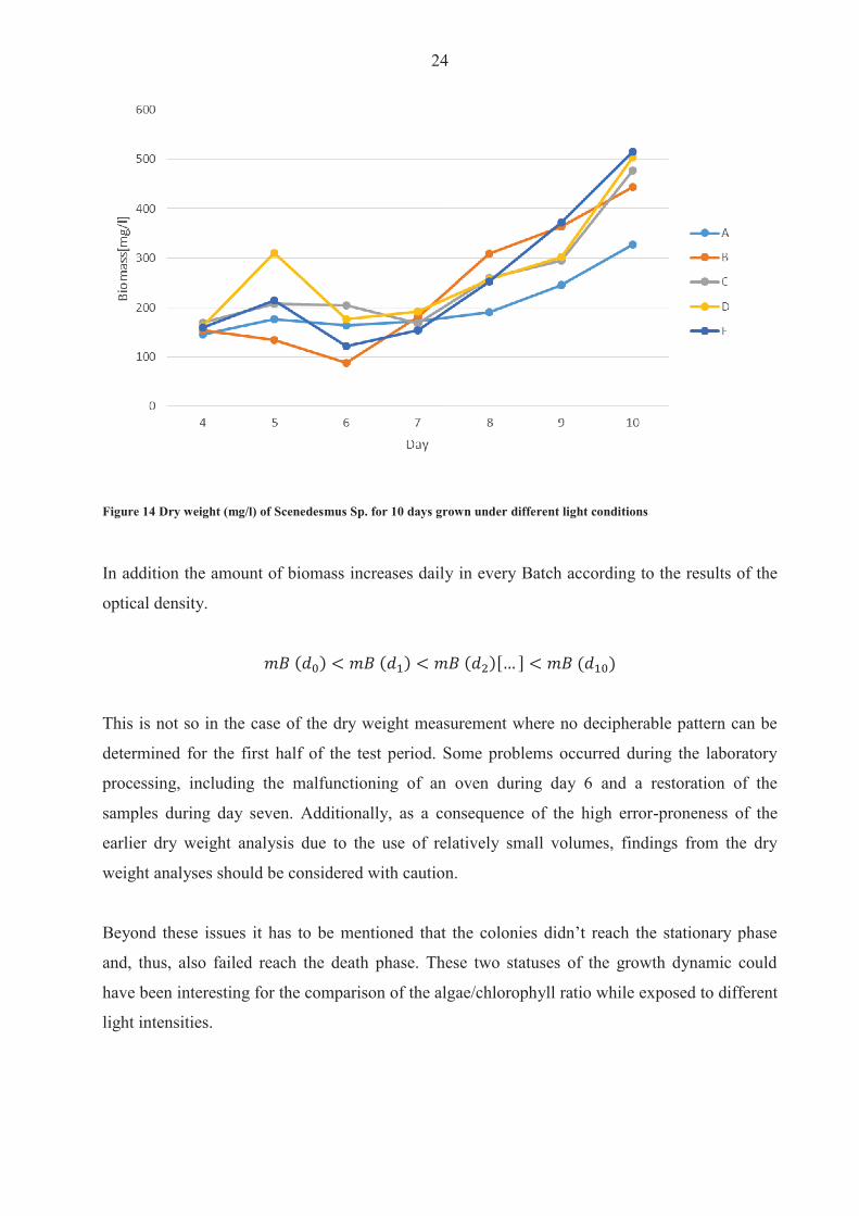
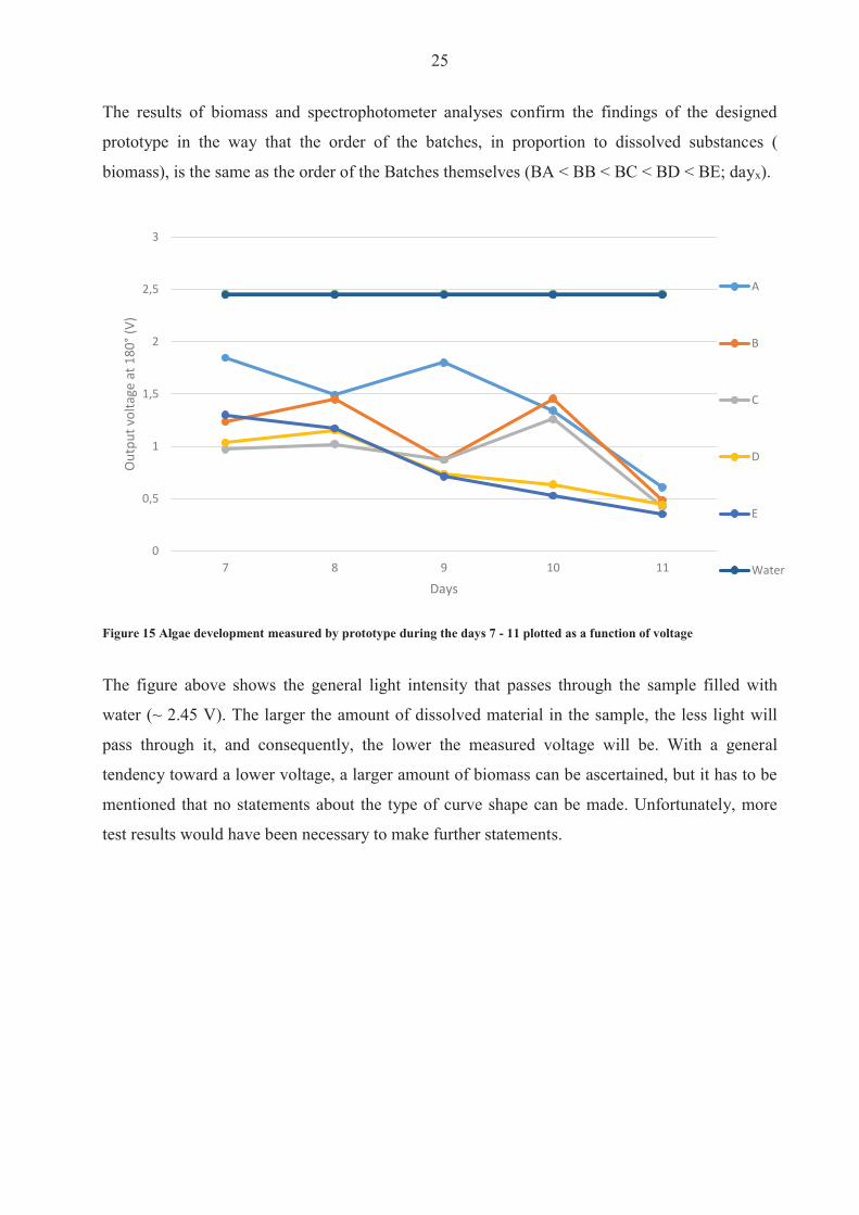
25
The results of biomass and spectrophotometer analyses confirm the findings of the designed
prototype in the way that the order of the batches in proportion to dissolved substances (
biomass) is the same as the order of the Batches themselves (BA lt BB lt BC lt BD lt BE dayx)
Figure 15 Algae development measured by prototype during the days 7 - 11 plotted as a function of voltage
The figure above shows the general light intensity that passes through the sample filled with
water (~ 245 V) The larger the amount of dissolved material in the sample the less light will
pass through it and consequently the lower the measured voltage will be With a general
tendency toward a lower voltage a larger amount of biomass can be ascertained but it has to be
mentioned that no statements about the type of curve shape can be made Unfortunately more
test results would have been necessary to make further statements
0
05
1
15
2
25
3
7 8 9 10 11
Outp
ut vo
ltage
at 1
80deg(
V)
Days
A
B
C
D
E
Water
26
32 Chlorophyll formation
After the chlorophyll-acetone mix is stored for 24 hours it is analyzed with a spectrophotometer
For the calculation of chlorophyll content according to Jeffrey amp Humphrey (1975) only some
wavelengths are important Nevertheless the chlorophyll was treated in the same way as the
algae and measurements were made in the range of 400 nm to 750 nm in order to determine
possible similarities
Figure 16 Chlorophyll (mgl) of Scenedesmus sp for 10 days grown under different illumination conditions
The concentration of total chlorophyll increases during the test The results show a steady growth
if expressed as the exponential regression curve (dotted lines) for Batches D and E (R = 09) A
better correlation is shown for a linear regression for Batches A and B (R = 09 instead of 076)
Batch C doesnrsquot show a strong correlation under either a linear (R = 072) or an exponential
growth (R = 076) assumption Many factors affect the results of the Chlorophyll measurement
Firstly the analyses are susceptible to mistakes made during the processing When removing 10
ml from the batches with a concentration of barely 1 mgL and using those samples in a cuvette
of 3 mL the amount of Chlorophyll is typically in a range of 0 ndash 10 μgmL Working with such
small quantities can lead to inaccuracies during processing in addition to errors made on behalf
of the measuring engine itself
Rsup2 = 07602
Rsup2 = 07602
Rsup2 = 09004
Rsup2 = 09037
Rsup2 = 07594
0
05
1
15
2
25
0 1 2 3 4 5 6 7 8 9 10 11
Chlo
roph
yll a
+b (m
gl)
Day
C
D
E
B
A
Expon (C)
Expon (C)
Expon (C)
Expon (D)
Expon (D)
Expon (E)
Linear (B)
Expon (A)
Linear (A)
27
Nevertheless we can make the assumption that the tendency (daily increase) makes sense The
results of the pilot engine show slightly decreasing curves At day 8 there is an obvious mistake
to declare This is not visible with regard to algae measurement at day 93 This leads to the
assumption of a mistake made during the preparing procedure with acetone Since the
abnormality can be found in all batches a mistake during the withdrawal can be ruled out
Figure 17 Chlorophyll development during the days 7 - 11 plotted as a function of voltage
A further problem is that the curves are not clearly separable They cross each other without
showing a decipherable trend with regard to which batch has the highest or the lowest
translucency (which would be proportional to the voltage) As a consequence these results
cannot provide information about the effect of different light irradiation and it is questionable
whether they can be used to make an assumption about chlorophyll accumulation
3 The spectrophotometer analyzes of chlorophyll is one day after due to the 24 hours storing of the samples
0
05
1
15
2
25
3
7 8 9 10 11
Outp
ut vo
ltage
at 1
80deg(
V)
Days
E
B
C
D
A
Water
28
33 Correlation of Algae and Chlorophyll growth The main rationale for using different light irradiation for the Batches was to determine the
relationship between algae growth and the Chlorophyll enhancement Hence interest lay beyond
simply examining the thesis that the concentration of Chlorophyll is directly linked to the algae
growth Furthermore there was interest in exploring whether a specific relationship existed
between the algae growth rate the exposure to light and the amount of chlorophyll produced
Figure 18 Collocation of AlgaeChlorophyll absorbance (by 665 nm) by a spectrophotometer for 11 days
Unfortunately an incomplete test phase (no algae growth until the stationary phase) was
responsible for a lack of results that could be used for further analysis Nevertheless the ratio of
Chlorophyll-to-Algae growth shows a decent progression (see also Table 4) There is no
evidence for a similar progression if the tests proceed for one or two weeks In theory the
chlorophyll concentration should increase more rapidly in the exponential phase (until now the
progress is best described as a linear growth) Furthermore the concentration of algae as well as
of chlorophyll from batch E should reach its maximum first followed by batch D C B A (in
this order) and continue at a stationary rate
BAA
lgae
BAC
hlBB
Alg
aeBB
Chl
BCA
lgae
BCC
hl
BDA
lgae
BDC
hl
BEA
lgae
BEC
hl
002040608
112141618
12
34
56
78
9 1011
BatchSubstrate
Abso
rban
ce
Days
BAAlgae
BAChl
BBAlgae
BBChl
BCAlgae
BCChl
BDAlgae
BDChl
BEAlgae
BEChl
29
Due to the issues described in the earlier chapters the results from analyses on biomass are less
convincing than those arising from the analyses of the spectrophotometer In addition and
contrary to the absorbance measurement the values of dry weight and calculated chlorophyll
correlate weakly in cases of batches with higher light saturation This may be due to inaccuracies
from the dry weight results or another reason could be the earlier start of a kind of exponential
growth for the chlorophyll while the results for the biomass donrsquot show an exponential increase
until the 7th day
Table 4 Overview of the results of biomass prototype and spectrophotometer analyzes
Substrate Biomass (mgl) ndash Dry weight and Chl Optical density (V) -
Prototype Absorbance - Spectrophotometer
Min Max R Min Max R Min Max R BAAlgae 146 327
092 185 061
- 013 156
094 BAChl 001 164 212 170 001 017 BBAlgae 154 444
085 124 049
- 013 169
089 BBChl 004 172 206 175 001 026 BCAlgae 170 478
078 097 042
- 012 170
082 BCChl 002 188 194 181 001 023 BDAlgae 162 504
068 104 044
- 011 172
094 BDChl 002 124 196 171 001 026 BEAlgae 160 515
066 130 035
- 009 175
097 BEChl 002 114 215 195 001 031 The less exciting results are unfortunately given by the Prototype Here no significant correlation
can be mentioned at all In contrast to the spectrophotometer these values are provided by the
direct transmission Therefore the highest solution has the lowest value because more light is
absorbed by the dissolved material which is in this case biomass (or pure chlorophyll) This
result is surprisingly disappointing because the tests performed beforehand with fluorescence
(realized by Leonardo M Rolim) show a straight dependency of proportional relationship
between percental solution and transmission (see Figure 19 below)
Fluorescein is a fluorescent dye from the group of the xanthene It was used for the previous tests
because itrsquos a non-biological and well known substance with which all unwished side effects of a
living system can be avoided during tests
30
Figure 19 Measuring points of concentration given in optical density from fluorescence (Rolim Heinen amp Huff 2014)
The graph shows the transmission by 180 degC as accomplished with the algae and chlorophyll
during this work The curve suggests a negative exponential trend This was also expected for the
new series of tests While a clear difference can be recorded in the case of fluorescein the values
of chlorophyll almost didnrsquot change This could be an effect of the high fluorescent impact of
fluorescence Due to the growth rate of chlorophyll (see Table 4 Chl Min and Max) which goes
from 001 gmL up to almost 18 gmL (180 times more) compared with the fluorescence which
goes from 001 gmL up to 03 gmL (30 times more) this is questionable since the concentration
difference is 5 times higher for pure chlorophyll a fluorescent pigment as well but the effect is
very little Nevertheless it could be an indication as to why results from the test were not as
expected
The analyses by the fluorimeter provides further interesting results The figure below presents
the results of chlorophyll for the 11th day The x-axis shows the input of the wave length
produced by the laser The excitation is visible on the y-axis while curves on the graph present
one specific wave length each between 400 and 800 nm (with an interval of 5 ie a new
measurement was performed for every 5 nm) In order to simplify the graphical presentation the
legend was omitted
31
Figure 20 Display of emission and excitation measured by the fluorimeter of day 11 for chlorophyll
The figure provides an important insight into the behavior of chlorophyll fluorescent The
formation on the bluish part of the light spectrum (270 ndash 430 nm) and the second cluster of peaks
between 650 and 675 nm are quite revealing The table below explains the most important
curves
Table 5 Legend of figure 16
Color wave length (nm) red 675 blue 670 gray 680
light green 665 orange 685
light blue 660 dark blue 690 dark green 695
These eight curves are explicitly mentioned because they have the highest response in the tested
emission spectrum Due to usually low concentrations of samples eg chlorophyll in μgml a
high response is vital The results of the other test days are equal They simply vary in the height
of excitation as a result of a higher concentration
0
200000
400000
600000
800000
1000000
1200000
1400000
1600000
300 325 350 375 400 425 450 475 500 525 550 575 600 625 650 675 700 725 750
Exita
tion
ampe
rage
at 9
0deg(m
A)
Emission wave lenght (nm)
32
Figure 21 Display of emission and excitation measured by the fluorimeter between the days 0 and 11 for chlorophyll (BA)
The daily difference of the excitation is presented above The course of the curves is equal and
just differs as mentioned before in the amount of ampere measured by the receptor The same
shape would be plotted by the other batches The only difference again would be the level of
excitation
The progression of the chlorophyll curves during the tests shows a permanent increase beginning
at day three An exponential correlation can be verified for the plotted curves Thus the results
from the fluorimeter are as expected before Still the problem as mentioned before of the
incomplete growth of the algae was responsible for a lack of further information which could
have been interesting
0
200000
400000
600000
800000
1000000
1200000
350 375 400 425 450 475 500 525 550 575 600 625 650 675 700 725 750
Excit
atio
n am
pera
ge a
t 90
deg(m
A)
Emission wave lenght (nm)
0
1
2
3
4
5
6
7
8
9
10
11
33
Figure 22 Trend of the chlorophyll excitation peaks during 11 days measured by the fluorimeter
In the following section the results from the algae analyses are explained One problem has to be
mentioned beforehand
The graph below shows the outcome from the last day Highly overlapping curves are visible
This is not caused by fluorescence but by the reflection of each wave length itself due to a high
solution The analyses made by the fluorimeter requires at least 30 minutes That it enough time
for the dissolved particle to settle down The x-axis can accordingly be viewed as a timeline
scale As more time passes by the reflection impact reduces
Rsup2 = 08453
0
200000
400000
600000
800000
1000000
1200000
1400000
1600000
1800000
2000000
0 2 4 6 8 10 12
Excit
atio
n am
pera
ge a
t 90
deg(m
A)
Days
660
665
430
405
375
Log (375)
34
Figure 23 Fluorimeter results of algae (BA day11)4
When the y-axis is limited to 100000 mA some other formations are visible Interestingly they
have the same shape as the curves of the chlorophyll which leads to the assumption that those
overlapped curves are indeed the fluorescent impact of the chlorophyll pigments
4 Every curve presents one wave length of the emission spectrum in an interval of five The legend is once more excluded due to a better overview
0
1000000
2000000
3000000
4000000
5000000
6000000
7000000
8000000
300 325 350 375 400 425 450 475 500 525 550 575 600 625 650 675 700 725 750
Excit
atio
n am
pera
ge a
t 90deg
(mA)
Emission wave lenght (nm)
35
Figure 24 Fluorimeter results of algae (BA day11) with limited y-axes up to 100000 mA5
On closer examination it can be interpreted that the higher curves (blue orange green dark
blue redhellip) are the same wavelengths as seen in the Table 5 Legend of figure 16rdquo The highest
response again is at 675 nm Measureing by a different wave length than 675 nm will cause
lower excitation The same happens in case of chlorophyll
The excitation is low in comparison with the results of the pure chlorophyll because the
chlorophyll is not separated from the cells which hinders the light from reaching the pigments
in addition to leaving the sample and stimulating the receptor
The comparison with the other batches and the analyses of the different days provides the same
results as for the chlorophyll That means the Excitation of BA(dx) lt BB(dx) lt BC(dx) lt BD(dx)
lt BE(dx) and the Excitation of BA(dx) lt BA(dx+1) BB(dx) lt BB(dx+1) BC(dx) lt BC(dx+1)
BD(dx) lt BD(dx+1) BE(dx) lt BE(dx+1)
5 The legend is once more excluded due to a better overview
0
10000
20000
30000
40000
50000
60000
70000
80000
90000
100000
300 325 350 375 400 425 450 475 500 525 550 575 600 625 650 675 700 725 750
Excit
atio
n am
pera
ge a
t 90
deg(m
A)
Emission wave lenght (nm)
36
4 Conclusiones
According to the results from the fluorimeter the algae growth and chlorophyll enhancement
appear to be as expected This leads to the question as to why the previous tests donrsquot have
similar outcomes The answer to this question and the reason why fluorimeters are used for low
quantities is the same They have a very high accuracy and are thus extremely efficient even
for low quantities Nevertheless they are extremely expensive and the main task of this project
was to determine whether it was possible to measure chlorophyll (pure or even intracellular) with
the prototype or if not to work out further steps for the development of the engine
The first step apart from the biological section is to make the engine more stable During the
project problems often occurred with regard to replication of results because small changes in the
electrical connection contributed to different outcomes while using the same sample This made
the testing more complicated and made unnecessary repetitions of measurement indispensable A
shell for the entire construction in which the electronic is fixed should solve this problem An
extension cable which leads to the measuring box together with a smaller diameter of the cell
itself would also be useful The laser and the two receptors should be installed separately from
the cell and waterproofed (plastic and glue should be sufficient) As a result the cell could be
introduced into a sample to measure which not only simplifies the procedure but it is also closer
to any practical application
The next action is the acquisition of the correct optical filter The results of the fluorimeter
suggest an optimal emission at 430 plusmn 10 nm while the excitation should be measured at 675 plusmn 10
nm The closer the measurement is to these wavelengths the higher the values of the results
Furthermore it was explained how other wave lengths overlap the fluorescence effect This can
be avoided by use of at least two filters one which filters the light of the laser and blocks out
every wavelength except for those in the range of eg 420 ndash 440 nm and a second filter which
allows for only the spectrum from 665 to 685 nm to pass
Nevertheless an upgrade of either the receptor or laser but probably both will be inevitable As
mentioned in the previous chapter the outcome of the 90deg measurement for algae and
chlorophyll is almost zero In actuality it has the same value as if measured with water which
means that the receptor is not able to recognize any approaching light On the other hand it may
37
be that the laser is too weak so that not enough light is injected In any case adjustment for the
right filter range should be the first step
When the filter and laserreceptor problems are solved a new test with fluorescence would make
sense At this stage it is important not only that the results are good for one series of tests but
also that they are repeatable Daily calibration of the engine is not only effortful and time-
consuming but it can also lead to variable results After good and stable results are achieved
with fluoresce a new test series with algae can be started Therefore it would be useful to create
a serial dilution of an algae culture which is already in the stationary phase and highly
concentrated If the results are suitable it can be continued with a serial dilution of those algae
Even if the results from the 90deg measurement are not satisfying a further test with pure
chlorophyll could be accomplished on condition that the results from the 180deg measurement are
decent
Only after all the described experiments have sufficient results should a new long-term test series
be started For this purpose no more than three batches should be installed with an intensity of
illumination between 3000 and 10000 lux The test duration should be approximately 30 days to
ensure that the culture passes through all growing and dying phases Tests performed with the
spectrophotometer can indicate a change of the growing conditions so that further and more
elaborated tests with the fluorimeter and biomass can be performed The measurement of
biomass should be sufficient if performed every three days (a daily testing during the exponential
phase would perhaps be useful) By using the fluorimeter care has to be taken so that the dilution
of the sample is large enough otherwise overlapping effects occur The analyses with the sensor
should be performed daily in order to get a consistent overview of the chlorophyllalgae ratio as
well as to gauge the accuracy of the sensor
38
5 Bibliography Boumlcker J (1979) Spektroskopie Instrumentelle Analytik mit Atom- und Molekuumllspektroskopie
(1 Edition Ausg) Wuumlrzburg Vogel Verlag und Druck GmbH amp Co
Hegewald P (2006) Scenedesmusndashlike algae of Ukraine Tsarenko E amp B Braband
Lehmann E W (1892) Uumlber ein Photometer Erlangen
Lourenccedilo S (2006) Cultivo de Microalgas Marinhas Princiacutepios e Aplicaccedilotildees
Luumlrling M (1999) The Smell of Water Grazer-Induced Colony Formation in Scenedesmus
Wageningen Pulz und Gross
Mills I Cvitaš T Homann K Kallay N amp Kuchitsu K (1993) Quantities Units and
Symbols in Physical Chemistry (Green Book)
Rolim L M Heinen A L amp Huff D D (2014) Desenvolvimento de sensor oacuteptico portaacutetil
para mediccedilatildeoes online de concentraccedilatildeo no cultivo de microalgas Porto Alegre
Rouilly V (2014) Schmidt W (2000) Optische Spektroskopie (Bd 2 Edition) Weinheim
WILEY-VCH Verlag GmbH
Unknown (1999) Photometer Spektrum Akademischer Verlag
Willows R D (2013) Structure of chlorophyll Organic Letters
Zander M (1981) Fluorimetrie Berlin-Heidelberg-New York Springer-Verlag
Internet sources Openwetwareorg
photometercom
teachingshuacuk
wikipediaorg
39
6 List of figures Figure 1 Pilot batch deployment 7
Figure 2 Relation between transmittance and absorbance 9
Figure 3 Structure of a photometer 10
Figure 4 Structure of a photometer with a dual-bean 12
Figure 5 Dual beam measuring method with only one photodetector 13
Figure 6 Common structure of a fluorimeter device 15
Figure 7 schematic diagram of the prototype sensor (left) and photo (right) 16
Figure 8 Filter ldquoStrawrdquo to eliminate unwished wave length 17
Figure 9 Chemical structure of chlorophyll 18
Figure 10 Sketch of algae growth dynamics 20
Figure 11 Progress of all 5 batches in a time interval of 11 days 21
Figure 13 By comparison absorbance between 400 nm and 750 nm of five batches at day 6 and 7
22
Figure 14 Progress of culture growth comparing Batch E (left) and A (right) during the 10 days
in comparison to the Absorbance 23
Figure 15 Dry weight (mgl) of Scenedesmus Sp for 10 days grown under different light
conditions 24
Figure 16 Algae development measured by prototype during the days 7 - 11 plotted as a function
of voltage 25
Figure 17 Chlorophyll (mgl) of Scenedesmus sp for 10 days grown under different illumination
conditions 26
Figure 18 Chlorophyll development during the days 7 - 11 plotted as a function of voltage 27
Figure 19 Collocation of AlgaeChlorophyll absorbance (by 665 nm) by a spectrophotometer for
11 days 28
Figure 20 Measuring points of concentration given in optical density from fluorescence 30
Figure 21 Display of emission and excitation measured by the fluorimeter of day 11 for
chlorophyll 31
Figure 22 Display of emission and excitation measured by the fluorimeter between the days 0
and 11 for chlorophyll (BA) 32
Figure 23 Trend of the chlorophyll excitation peaks during 11 days measured by the fluorimeter
33
Figure 24 Fluorimeter results of algae (BA day11) 34
Figure 25 Fluorimeter results of algae (BA day11) with limited y-axes up to 100000 mA 35
40
7 List of tables Table 1 Composition of algae supplementary medium 6
Table 2 Specifications of the used T80 spectrophotometer 11
Table 3 Specifications of the used FluoroMaxR Fluorimeter 13
Table 4 Overview of the results of biomass prototype and spectrophotometer analyzes 29
Table 5 Legend of figure 16 31
41
Declaration of Authorship I hereby certify that this work has been composed by me and is based on my own work
unless stated otherwise No other person`s work has been used without due
acknowledgement in this report All references and verbatim extracts have been quoted
and all sources of information including graphs and data sets have been specifically
acknowledged
______________________ ________________________ Ort Datum Signature
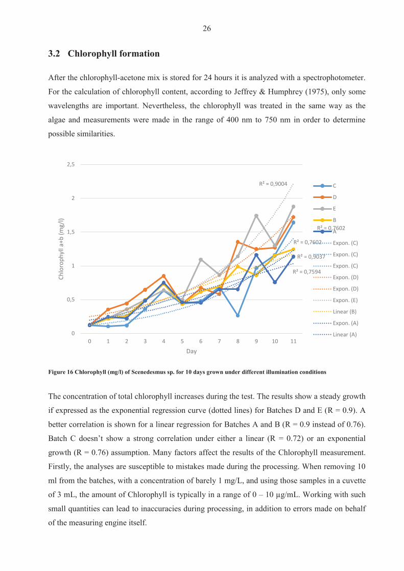
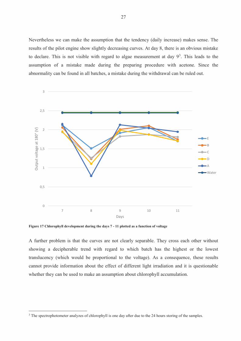
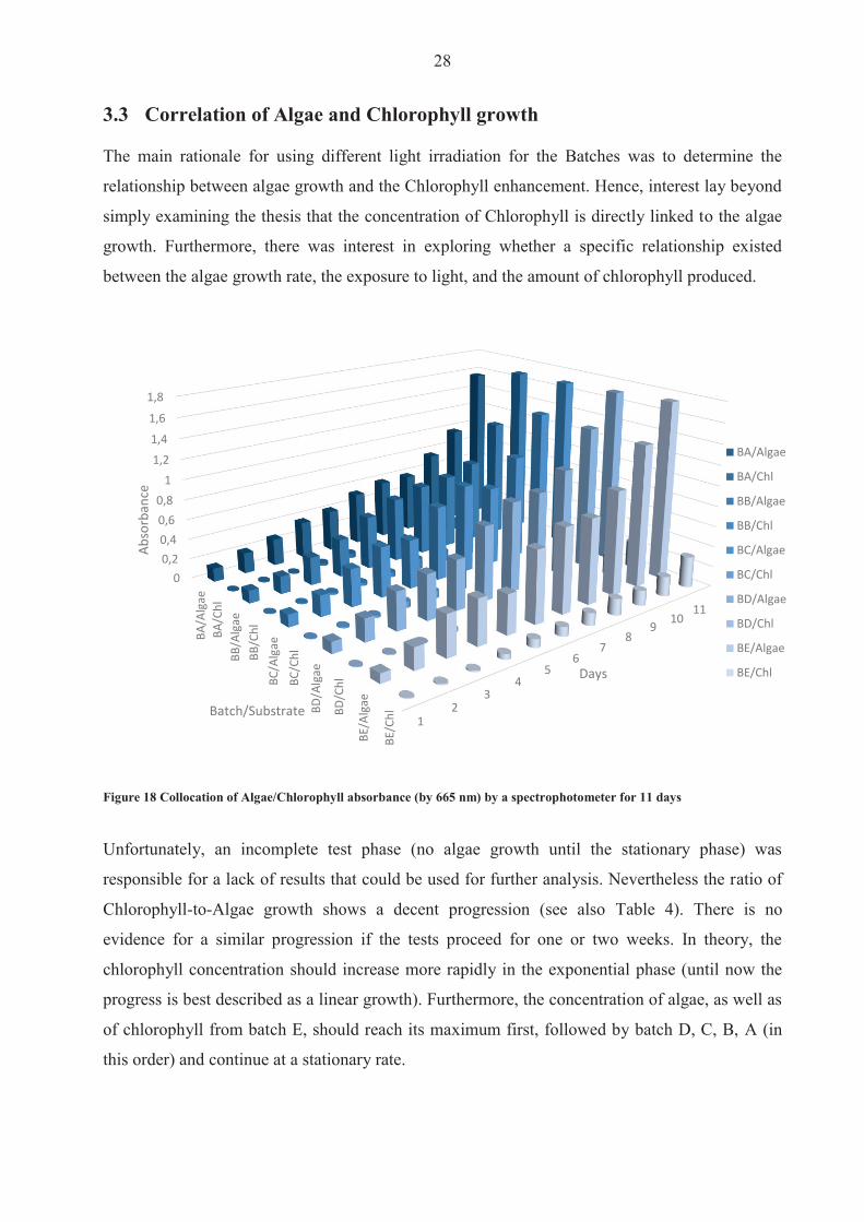
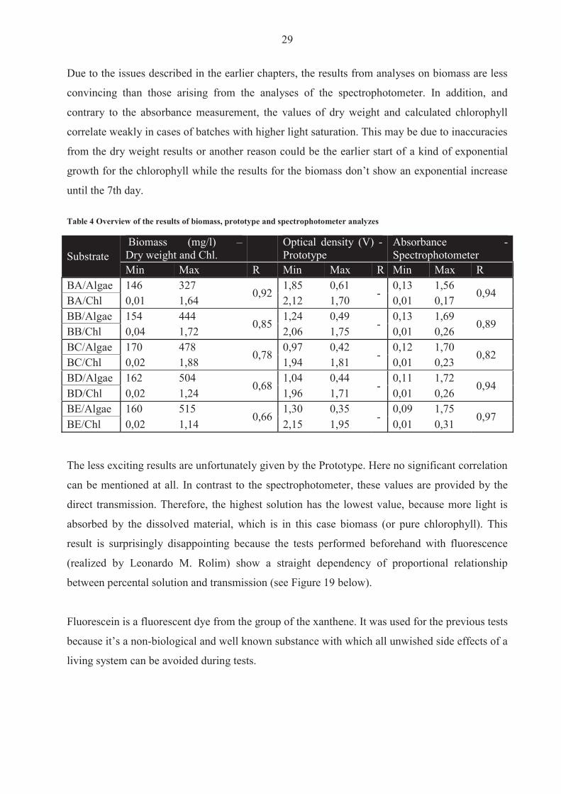
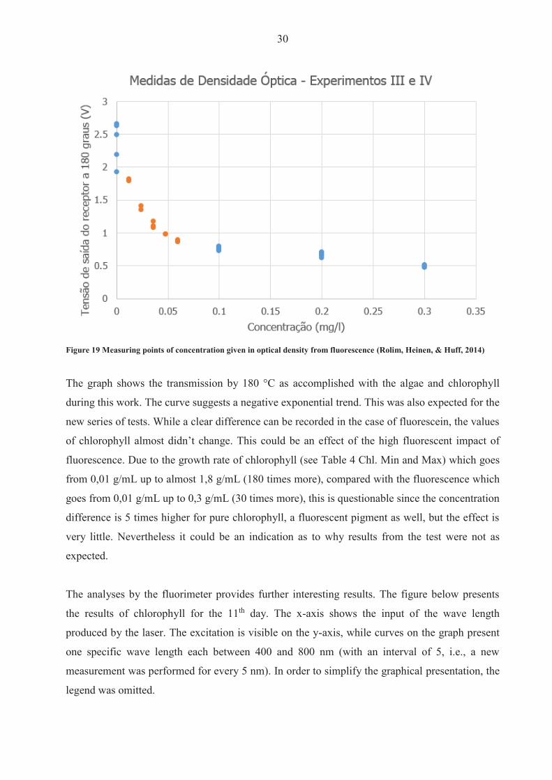
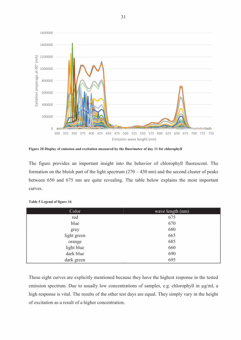
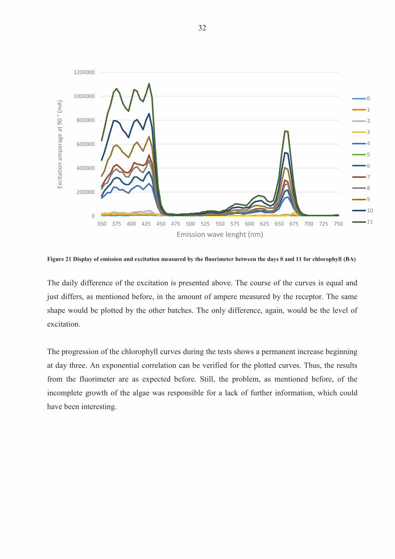
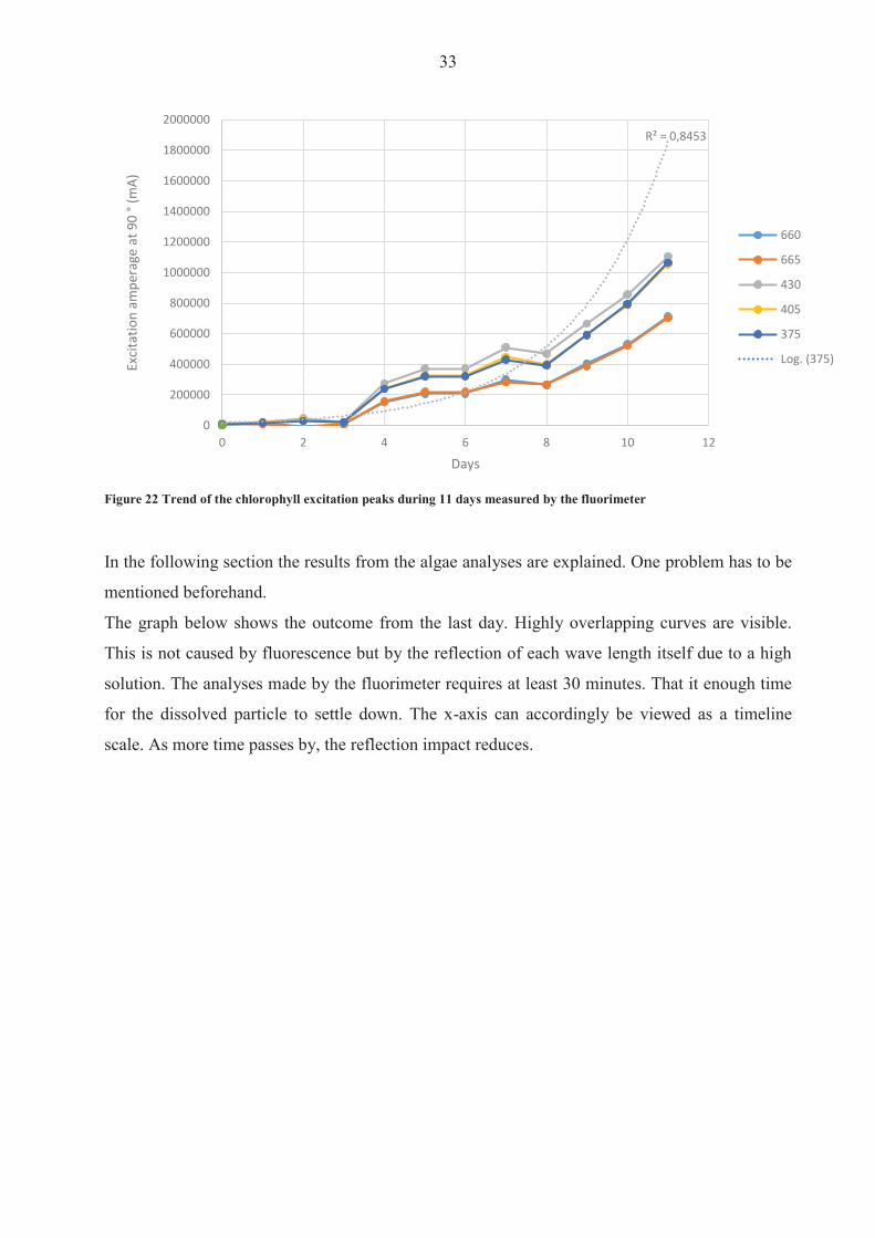
33
Figure 22 Trend of the chlorophyll excitation peaks during 11 days measured by the fluorimeter
In the following section the results from the algae analyses are explained One problem has to be
mentioned beforehand
The graph below shows the outcome from the last day Highly overlapping curves are visible
This is not caused by fluorescence but by the reflection of each wave length itself due to a high
solution The analyses made by the fluorimeter requires at least 30 minutes That it enough time
for the dissolved particle to settle down The x-axis can accordingly be viewed as a timeline
scale As more time passes by the reflection impact reduces
Rsup2 = 08453
0
200000
400000
600000
800000
1000000
1200000
1400000
1600000
1800000
2000000
0 2 4 6 8 10 12
Excit
atio
n am
pera
ge a
t 90
deg(m
A)
Days
660
665
430
405
375
Log (375)
34
Figure 23 Fluorimeter results of algae (BA day11)4
When the y-axis is limited to 100000 mA some other formations are visible Interestingly they
have the same shape as the curves of the chlorophyll which leads to the assumption that those
overlapped curves are indeed the fluorescent impact of the chlorophyll pigments
4 Every curve presents one wave length of the emission spectrum in an interval of five The legend is once more excluded due to a better overview
0
1000000
2000000
3000000
4000000
5000000
6000000
7000000
8000000
300 325 350 375 400 425 450 475 500 525 550 575 600 625 650 675 700 725 750
Excit
atio
n am
pera
ge a
t 90deg
(mA)
Emission wave lenght (nm)
35
Figure 24 Fluorimeter results of algae (BA day11) with limited y-axes up to 100000 mA5
On closer examination it can be interpreted that the higher curves (blue orange green dark
blue redhellip) are the same wavelengths as seen in the Table 5 Legend of figure 16rdquo The highest
response again is at 675 nm Measureing by a different wave length than 675 nm will cause
lower excitation The same happens in case of chlorophyll
The excitation is low in comparison with the results of the pure chlorophyll because the
chlorophyll is not separated from the cells which hinders the light from reaching the pigments
in addition to leaving the sample and stimulating the receptor
The comparison with the other batches and the analyses of the different days provides the same
results as for the chlorophyll That means the Excitation of BA(dx) lt BB(dx) lt BC(dx) lt BD(dx)
lt BE(dx) and the Excitation of BA(dx) lt BA(dx+1) BB(dx) lt BB(dx+1) BC(dx) lt BC(dx+1)
BD(dx) lt BD(dx+1) BE(dx) lt BE(dx+1)
5 The legend is once more excluded due to a better overview
0
10000
20000
30000
40000
50000
60000
70000
80000
90000
100000
300 325 350 375 400 425 450 475 500 525 550 575 600 625 650 675 700 725 750
Excit
atio
n am
pera
ge a
t 90
deg(m
A)
Emission wave lenght (nm)
36
4 Conclusiones
According to the results from the fluorimeter the algae growth and chlorophyll enhancement
appear to be as expected This leads to the question as to why the previous tests donrsquot have
similar outcomes The answer to this question and the reason why fluorimeters are used for low
quantities is the same They have a very high accuracy and are thus extremely efficient even
for low quantities Nevertheless they are extremely expensive and the main task of this project
was to determine whether it was possible to measure chlorophyll (pure or even intracellular) with
the prototype or if not to work out further steps for the development of the engine
The first step apart from the biological section is to make the engine more stable During the
project problems often occurred with regard to replication of results because small changes in the
electrical connection contributed to different outcomes while using the same sample This made
the testing more complicated and made unnecessary repetitions of measurement indispensable A
shell for the entire construction in which the electronic is fixed should solve this problem An
extension cable which leads to the measuring box together with a smaller diameter of the cell
itself would also be useful The laser and the two receptors should be installed separately from
the cell and waterproofed (plastic and glue should be sufficient) As a result the cell could be
introduced into a sample to measure which not only simplifies the procedure but it is also closer
to any practical application
The next action is the acquisition of the correct optical filter The results of the fluorimeter
suggest an optimal emission at 430 plusmn 10 nm while the excitation should be measured at 675 plusmn 10
nm The closer the measurement is to these wavelengths the higher the values of the results
Furthermore it was explained how other wave lengths overlap the fluorescence effect This can
be avoided by use of at least two filters one which filters the light of the laser and blocks out
every wavelength except for those in the range of eg 420 ndash 440 nm and a second filter which
allows for only the spectrum from 665 to 685 nm to pass
Nevertheless an upgrade of either the receptor or laser but probably both will be inevitable As
mentioned in the previous chapter the outcome of the 90deg measurement for algae and
chlorophyll is almost zero In actuality it has the same value as if measured with water which
means that the receptor is not able to recognize any approaching light On the other hand it may
37
be that the laser is too weak so that not enough light is injected In any case adjustment for the
right filter range should be the first step
When the filter and laserreceptor problems are solved a new test with fluorescence would make
sense At this stage it is important not only that the results are good for one series of tests but
also that they are repeatable Daily calibration of the engine is not only effortful and time-
consuming but it can also lead to variable results After good and stable results are achieved
with fluoresce a new test series with algae can be started Therefore it would be useful to create
a serial dilution of an algae culture which is already in the stationary phase and highly
concentrated If the results are suitable it can be continued with a serial dilution of those algae
Even if the results from the 90deg measurement are not satisfying a further test with pure
chlorophyll could be accomplished on condition that the results from the 180deg measurement are
decent
Only after all the described experiments have sufficient results should a new long-term test series
be started For this purpose no more than three batches should be installed with an intensity of
illumination between 3000 and 10000 lux The test duration should be approximately 30 days to
ensure that the culture passes through all growing and dying phases Tests performed with the
spectrophotometer can indicate a change of the growing conditions so that further and more
elaborated tests with the fluorimeter and biomass can be performed The measurement of
biomass should be sufficient if performed every three days (a daily testing during the exponential
phase would perhaps be useful) By using the fluorimeter care has to be taken so that the dilution
of the sample is large enough otherwise overlapping effects occur The analyses with the sensor
should be performed daily in order to get a consistent overview of the chlorophyllalgae ratio as
well as to gauge the accuracy of the sensor
38
5 Bibliography Boumlcker J (1979) Spektroskopie Instrumentelle Analytik mit Atom- und Molekuumllspektroskopie
(1 Edition Ausg) Wuumlrzburg Vogel Verlag und Druck GmbH amp Co
Hegewald P (2006) Scenedesmusndashlike algae of Ukraine Tsarenko E amp B Braband
Lehmann E W (1892) Uumlber ein Photometer Erlangen
Lourenccedilo S (2006) Cultivo de Microalgas Marinhas Princiacutepios e Aplicaccedilotildees
Luumlrling M (1999) The Smell of Water Grazer-Induced Colony Formation in Scenedesmus
Wageningen Pulz und Gross
Mills I Cvitaš T Homann K Kallay N amp Kuchitsu K (1993) Quantities Units and
Symbols in Physical Chemistry (Green Book)
Rolim L M Heinen A L amp Huff D D (2014) Desenvolvimento de sensor oacuteptico portaacutetil
para mediccedilatildeoes online de concentraccedilatildeo no cultivo de microalgas Porto Alegre
Rouilly V (2014) Schmidt W (2000) Optische Spektroskopie (Bd 2 Edition) Weinheim
WILEY-VCH Verlag GmbH
Unknown (1999) Photometer Spektrum Akademischer Verlag
Willows R D (2013) Structure of chlorophyll Organic Letters
Zander M (1981) Fluorimetrie Berlin-Heidelberg-New York Springer-Verlag
Internet sources Openwetwareorg
photometercom
teachingshuacuk
wikipediaorg
39
6 List of figures Figure 1 Pilot batch deployment 7
Figure 2 Relation between transmittance and absorbance 9
Figure 3 Structure of a photometer 10
Figure 4 Structure of a photometer with a dual-bean 12
Figure 5 Dual beam measuring method with only one photodetector 13
Figure 6 Common structure of a fluorimeter device 15
Figure 7 schematic diagram of the prototype sensor (left) and photo (right) 16
Figure 8 Filter ldquoStrawrdquo to eliminate unwished wave length 17
Figure 9 Chemical structure of chlorophyll 18
Figure 10 Sketch of algae growth dynamics 20
Figure 11 Progress of all 5 batches in a time interval of 11 days 21
Figure 13 By comparison absorbance between 400 nm and 750 nm of five batches at day 6 and 7
22
Figure 14 Progress of culture growth comparing Batch E (left) and A (right) during the 10 days
in comparison to the Absorbance 23
Figure 15 Dry weight (mgl) of Scenedesmus Sp for 10 days grown under different light
conditions 24
Figure 16 Algae development measured by prototype during the days 7 - 11 plotted as a function
of voltage 25
Figure 17 Chlorophyll (mgl) of Scenedesmus sp for 10 days grown under different illumination
conditions 26
Figure 18 Chlorophyll development during the days 7 - 11 plotted as a function of voltage 27
Figure 19 Collocation of AlgaeChlorophyll absorbance (by 665 nm) by a spectrophotometer for
11 days 28
Figure 20 Measuring points of concentration given in optical density from fluorescence 30
Figure 21 Display of emission and excitation measured by the fluorimeter of day 11 for
chlorophyll 31
Figure 22 Display of emission and excitation measured by the fluorimeter between the days 0
and 11 for chlorophyll (BA) 32
Figure 23 Trend of the chlorophyll excitation peaks during 11 days measured by the fluorimeter
33
Figure 24 Fluorimeter results of algae (BA day11) 34
Figure 25 Fluorimeter results of algae (BA day11) with limited y-axes up to 100000 mA 35
40
7 List of tables Table 1 Composition of algae supplementary medium 6
Table 2 Specifications of the used T80 spectrophotometer 11
Table 3 Specifications of the used FluoroMaxR Fluorimeter 13
Table 4 Overview of the results of biomass prototype and spectrophotometer analyzes 29
Table 5 Legend of figure 16 31
41
Declaration of Authorship I hereby certify that this work has been composed by me and is based on my own work
unless stated otherwise No other person`s work has been used without due
acknowledgement in this report All references and verbatim extracts have been quoted
and all sources of information including graphs and data sets have been specifically
acknowledged
______________________ ________________________ Ort Datum Signature
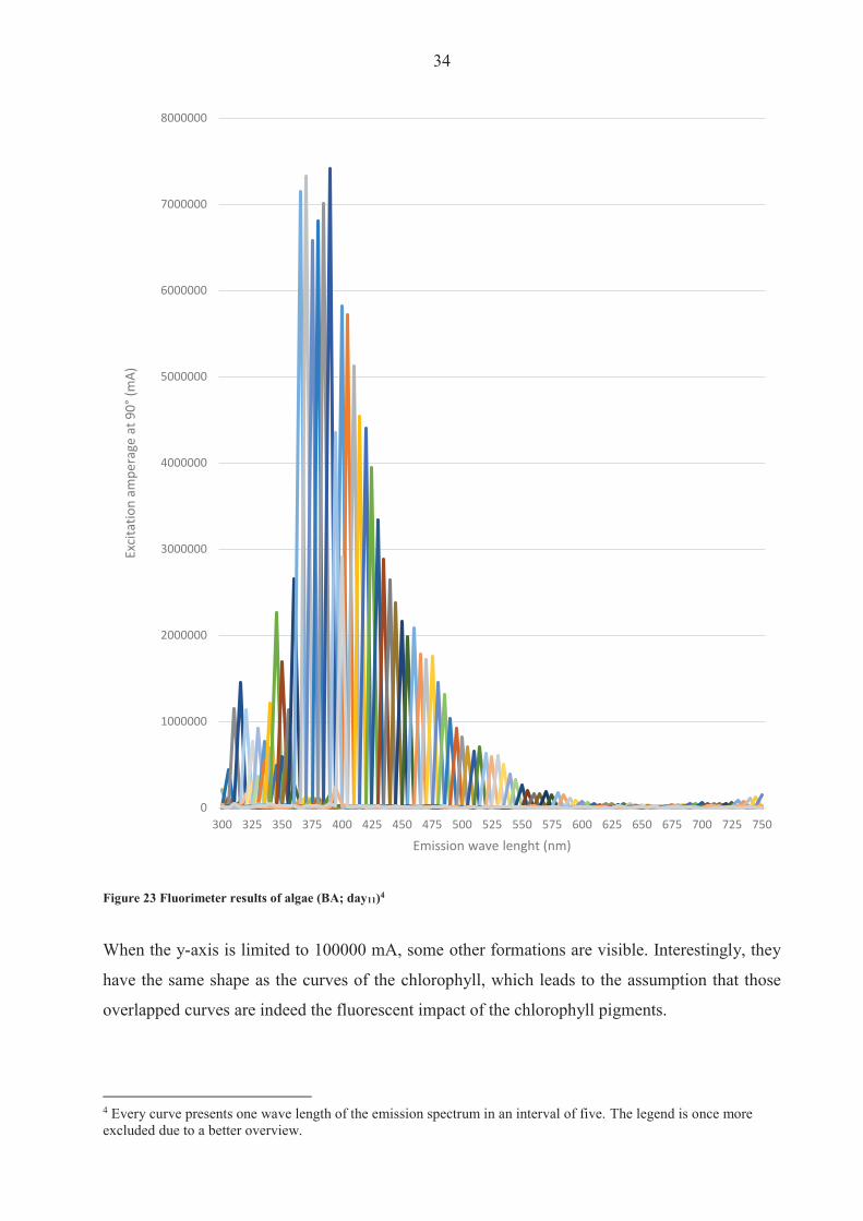
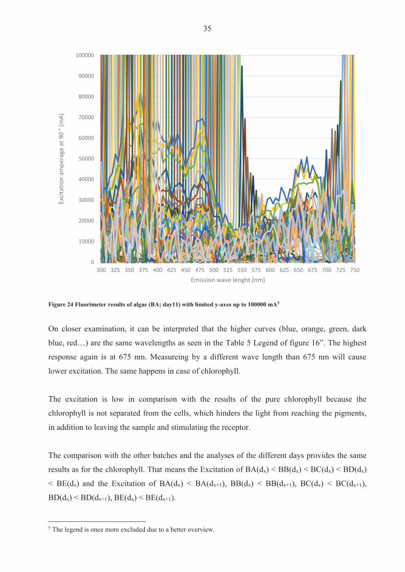