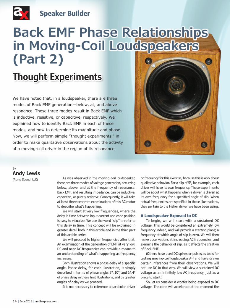
We have noted that, in a loudspeaker, there are three modes of Back EMF generation—below, at, and above resonance. These three modes result in Back EMF which is inductive, resistive, or capacitive, respectively. We explained how to identify Back EMF in each of these modes, and how to determine its magnitude and phase. Now, we will perform simple “thought experiments,” in order to make qualitative observations about the activity of a moving-coil driver in the region of its resonance.

ax Speaker Builder

14 | June 2018 | audioxpress.com

As was observed in the moving-coil loudspeaker, there are three modes of voltage generation, occurring below, above, and at the frequency of resonance. Back EMF, and resulting impedance, can be inductive, capacitive, or purely resistive. Consequently, it will take at least three separate examinations of this AC motor to describe what’s happening.

We will start at very low frequencies, where the delay in time between input current and cone position is easy to visualize. We use the word “slip” to refer to this delay in time. This concept will be explained in greater detail both in this article and in the third part of this article series.

We will proceed to higher frequencies after that. An examination of the generation of EMF at very low, DC and near-DC frequencies can provide a means to an understanding of what’s happening as frequency increases.

Each illustration shows a phase delay of a specific angle. Phase delay, for each illustration, is simply described in terms of phase angle: 5°, 10°, and 14.4° of phase delay in these first illustrations, and by greater angles of delay as we proceed.

It is not necessary to reference a particular driver

or frequency for this exercise, because this is only about qualitative behavior. For a slip of 5°, for example, each driver will have its own frequency. These experiments will be about what happens when a driver is driven at its own frequency for a specified angle of slip. When actual frequencies are specified in these illustrations, they pertain to the Fisher driver we have been using.

A Loudspeaker Exposed to DCTo begin, we will start with a sustained DC

voltage. This would be considered an extremely low frequency indeed, and will provide a starting place; a frequency at which angle of slip is zero. We will then make observations at increasing AC frequencies, and examine the behavior of slip, as it affects the creation of Back EMF.

(Others have used DC spikes or pulses as tools for testing moving-coil loudspeakers[1] and have drawn certain inferences from their observations. We will not use DC in that way. We will view a sustained DC voltage as an infinitely low AC frequency, just as a place to start.)

So, let us consider a woofer being exposed to DC voltage. The cone will accelerate at the moment the

By

Andy Lewis(Acme Sound, LLC)

Back EMF Phase Relationships in Moving-Coil Loudspeakers (Part 2)Thought Experiments

audioxpress.com | June 2018 | 15

voltage is applied, and the position of the cone will, for a short time, lag behind the resulting DC current (and force), as its mass is accelerated. As it changes position, it comes to its point of equilibrium for a given current, and its position remains constant—meaning velocity is zero. This point of equilibrium is the position at which the motor force on the voice coil is equal to the restoring spring force of the woofer’s suspension.

Current continues to flow at this point of equilibrium, even though the cone is not moving. Because cone velocity at this point of equilibrium is zero, there is no reverse voltage being generated. A motor force, as a result of this DC current still exists, but because it is opposed by an equal but opposite spring force, due to the speaker’s compliance, velocity is zero.

When exposed to DC, the unit’s impedance can be calculated, just as with AC. The impedance is equal to DC resistance plus Back EMF. Since velocity is zero, Back EMF is also zero. Therefore, the impedance at this (zero) frequency is equal to the DC resistance of the voice coil.

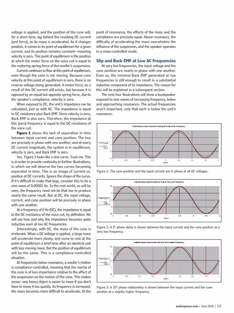
Figure 1 shows the lack of separation in time between input current and cone position. The two are precisely in phase with one another, and at every DC current magnitude, the system is in equilibrium, velocity is zero, and Back EMF is zero.

Yes, Figure 1 looks like a sine curve. Trust me. This is in order to provide continuity to further illustrations, in which we will observe the two curves becoming separated in time. This is an image of current vs. position at DC currents. Ignore the shape of the curve. If it’s difficult to make that leap, consider this to be a sine wave of 0.00001 Hz. In the real world, as will be seen, the frequency need not be that low to produce nearly the same result. But at DC, the input voltage, current, and cone position will be precisely in phase with one another.

At a frequency of 0 Hz (DC), the impedance is equal to the DC resistance of the voice coil, by definition. We will see how and why the impedance becomes quite inductive even at low AC frequencies.

Interestingly, with DC, the mass of the cone is irrelevant. When a DC voltage is applied, a large mass will accelerate more slowly, and come to rest at the point of equilibrium a brief time after an identical unit with less moving mass. But the position of equilibrium will be the same. This is a compliance-controlled situation.

At frequencies below resonance, a woofer’s motion is compliance-controlled, meaning that the inertia of the cone is of less importance relative to the effect of the suspension on the motion of the cone. This makes sense—any heavy object is easier to move if you don’t have to move it too quickly. As frequency is increased, the mass becomes more difficult to accelerate. At the

point of resonance, the effects of the mass and the compliance are precisely equal. Above resonance, the difficulty of accelerating the mass overwhelms the influence of the suspension, and the speaker operates in a mass-controlled mode.

Slip and Back EMF at Low AC FrequenciesAt very low frequencies, the input voltage and the

cone position are nearly in phase with one another. Even so, the minimal Back EMF generated at low frequencies is still enough to result in a substantial inductive component of its impedance. The reason for this will be explained in a subsequent section.

The next four illustrations will show a loudspeaker exposed to sine waves of increasing frequency, below and approaching resonance. The actual frequencies aren’t important, only that each is below the unit’s resonance.

Figure 1: The cone position and the input current are in phase at all DC voltages.

Figure 2: A 5° phase delay is shown between the input current and the cone position at a very low frequency.

Figure 3: A 10° phase relationship is shown between the input current and the cone position at a slightly higher frequency.

ax Speaker Builder

16 | June 2018 | audioxpress.com

We don’t need to specify a specific frequency, or a specific driver. These illustrations are a qualitative representation of the delay in time, or phase angle, between the input current and the resulting position of the cone. As was mentioned, each driver will have its own frequencies at which it exhibits any of these specific angles of slip.

With pure DC, input current and position are in phase with one another, and slip is zero. But as frequency is increased, cone position lags behind input current due to inertia, as slip increases, in turn. Therefore, the two curves begin to exhibit a separation in time.

We will gradually increase the frequency from zero (DC), and examine the position of the cone, relative to input current, below resonance. Even at extremely low frequencies, it’s easy to observe the slip graphically.

Which low frequency should we illustrate? Let us arbitrarily use the frequency at which the angle of slip is 5° as shown in Figure 2.

The third part of this article series will show how to calculate the angle of slip for a given Frequency. For now, we will graphically illustrate the behavior.

Referring to the Fisher woofer we discussed in the first part of the article series (audioXpress, May 2018), it can be calculated that the frequency at which the

phase delay between the input current and the cone position is 5°, is roughly 12 Hz. Again, that’s specific to this woofer. Each driver will have its own frequency of 5° slip.

As we increase the frequency slightly more, the phase delay between the input current and the slip increases to 10° (see Figure 3). This 10° slip corresponds to an input frequency of roughly 19 Hz using our Fisher woofer. As was said, each moving-coil driver will have its own frequency for a specific amount of slip.

As frequency is increased from near-DC, slip increases, in turn, because the moving mass and its acceleration remain constant as the period decreases. And therefore, the moving mass lags farther behind the input current, in Newtonian fashion:

F = ma

As frequency increases, so does angle of slip. It’s intuitively obvious, when viewed this way, and it’s important to gaining an understanding of the bigger picture.

Slip At Test Frequency f1 Figure 2 and Figure 3 illustrate the trend as

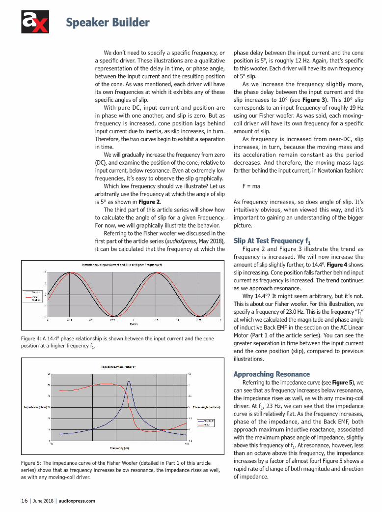
frequency is increased. We will now increase the amount of slip slightly further, to 14.4°. Figure 4 shows slip increasing. Cone position falls farther behind input current as frequency is increased. The trend continues as we approach resonance.

Why 14.4°? It might seem arbitrary, but it’s not. This is about our Fisher woofer. For this illustration, we specify a frequency of 23.0 Hz. This is the frequency “f1” at which we calculated the magnitude and phase angle of inductive Back EMF in the section on the AC Linear Motor (Part 1 of the article series). You can see the greater separation in time between the input current and the cone position (slip), compared to previous illustrations.

Approaching ResonanceReferring to the impedance curve (see Figure 5), we

can see that as frequency increases below resonance, the impedance rises as well, as with any moving-coil driver. At f1, 23 Hz, we can see that the impedance curve is still relatively flat. As the frequency increases, phase of the impedance, and the Back EMF, both approach maximum inductive reactance, associated with the maximum phase angle of impedance, slightly above this frequency of f1. At resonance, however, less than an octave above this frequency, the impedance increases by a factor of almost four! Figure 5 shows a rapid rate of change of both magnitude and direction of impedance.

Figure 4: A 14.4° phase relationship is shown between the input current and the cone position at a higher frequency f1.

Figure 5: The impedance curve of the Fisher Woofer (detailed in Part 1 of this article series) shows that as frequency increases below resonance, the impedance rises as well, as with any moving-coil driver.

audioxpress.com | June 2018 | 17

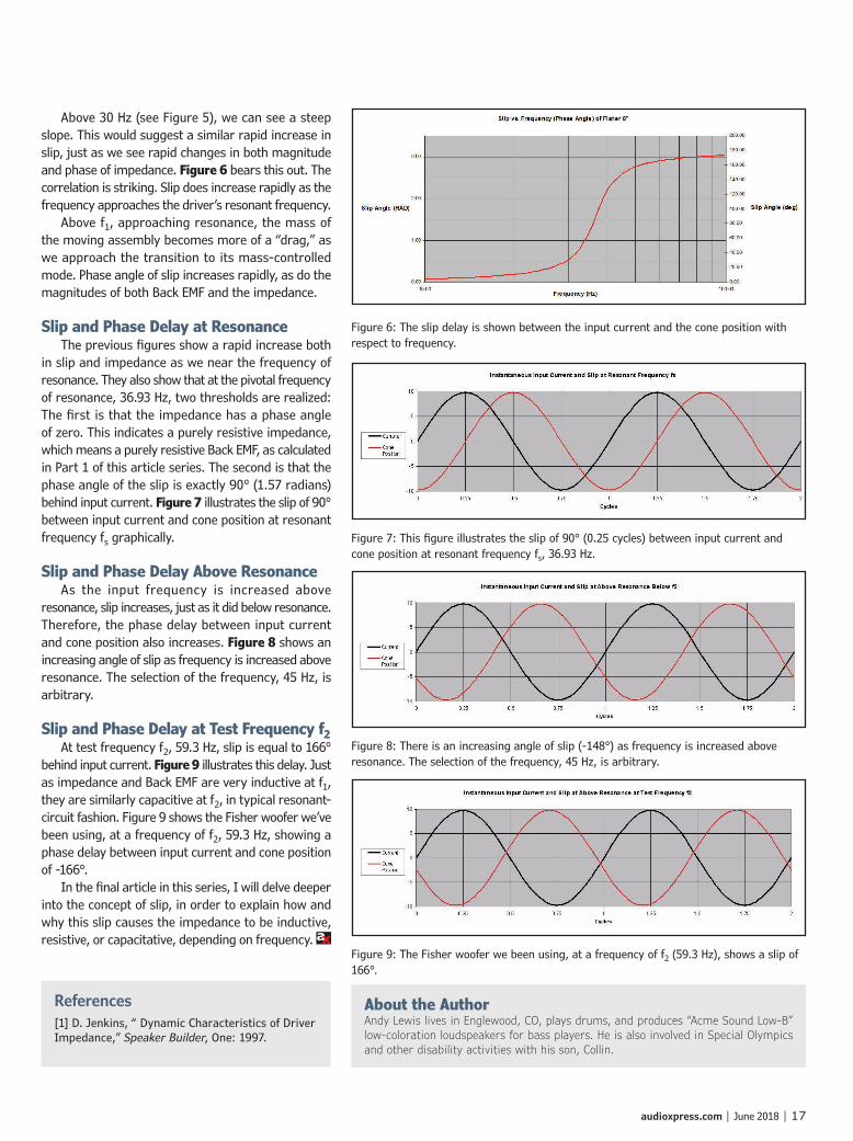
Above 30 Hz (see Figure 5), we can see a steep slope. This would suggest a similar rapid increase in slip, just as we see rapid changes in both magnitude and phase of impedance. Figure 6 bears this out. The correlation is striking. Slip does increase rapidly as the frequency approaches the driver’s resonant frequency.

Above f1, approaching resonance, the mass of the moving assembly becomes more of a “drag,” as we approach the transition to its mass-controlled mode. Phase angle of slip increases rapidly, as do the magnitudes of both Back EMF and the impedance.

Slip and Phase Delay at Resonance The previous figures show a rapid increase both

in slip and impedance as we near the frequency of resonance. They also show that at the pivotal frequency of resonance, 36.93 Hz, two thresholds are realized: The first is that the impedance has a phase angle of zero. This indicates a purely resistive impedance, which means a purely resistive Back EMF, as calculated in Part 1 of this article series. The second is that the phase angle of the slip is exactly 90° (1.57 radians) behind input current. Figure 7 illustrates the slip of 90° between input current and cone position at resonant frequency fs graphically.

Slip and Phase Delay Above Resonance As the input frequency is increased above

resonance, slip increases, just as it did below resonance. Therefore, the phase delay between input current and cone position also increases. Figure 8 shows an increasing angle of slip as frequency is increased above resonance. The selection of the frequency, 45 Hz, is arbitrary.

Slip and Phase Delay at Test Frequency f2At test frequency f2, 59.3 Hz, slip is equal to 166°

behind input current. Figure 9 illustrates this delay. Just as impedance and Back EMF are very inductive at f1, they are similarly capacitive at f2, in typical resonant-circuit fashion. Figure 9 shows the Fisher woofer we’ve been using, at a frequency of f2, 59.3 Hz, showing a phase delay between input current and cone position of -166°.

In the final article in this series, I will delve deeper into the concept of slip, in order to explain how and why this slip causes the impedance to be inductive, resistive, or capacitative, depending on frequency. ax

Figure 6: The slip delay is shown between the input current and the cone position with respect to frequency.

Figure 7: This figure illustrates the slip of 90° (0.25 cycles) between input current and cone position at resonant frequency fs, 36.93 Hz.

Figure 8: There is an increasing angle of slip (-148°) as frequency is increased above resonance. The selection of the frequency, 45 Hz, is arbitrary.

Figure 9: The Fisher woofer we been using, at a frequency of f2 (59.3 Hz), shows a slip of 166°.

References[1] D. Jenkins, “ Dynamic Characteristics of Driver Impedance,” Speaker Builder, One: 1997.

About the AuthorAndy Lewis lives in Englewood, CO, plays drums, and produces “Acme Sound Low-B” low-coloration loudspeakers for bass players. He is also involved in Special Olympics and other disability activities with his son, Collin.