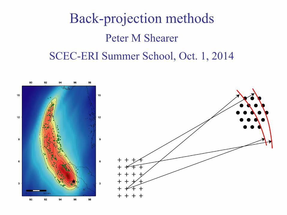
Back-projection methods

Peter M Shearer SCEC-ERI Summer School, Oct. 1, 2014

http://igppweb.ucsd.edu/~shearer/SCECERI/

Back-projection is a very intuitive idea and can be related to: • Earthquake location • Time reversal • Beam-forming and array processing • Migration in reflection seismology • Adjoint methods

A

B

C

North

East

Earthquake!

Seismic waves recorded at three stations:

Where did it happen?

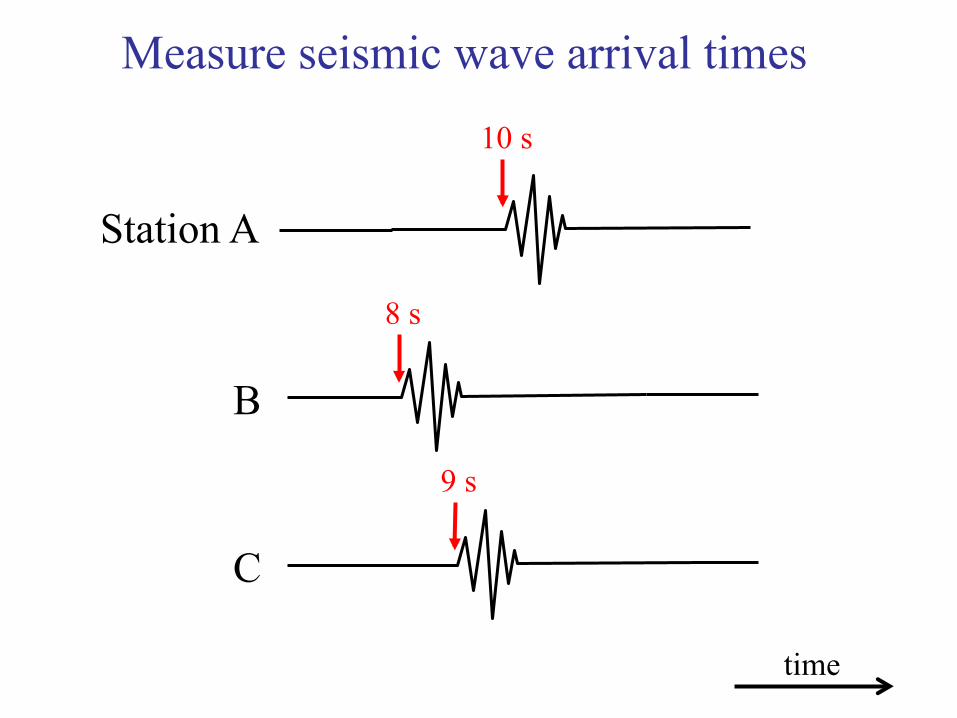
Measure seismic wave arrival times

Station A

B

C

time

10 s

9 s

8 s

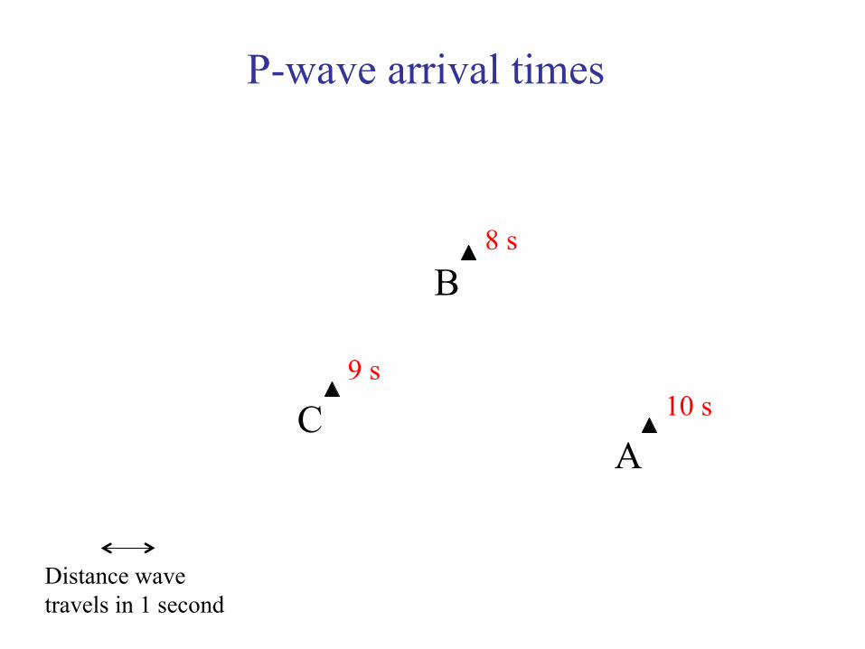
A

B

C

8 s

9 s 10 s

P-wave arrival times

Distance wave travels in 1 second

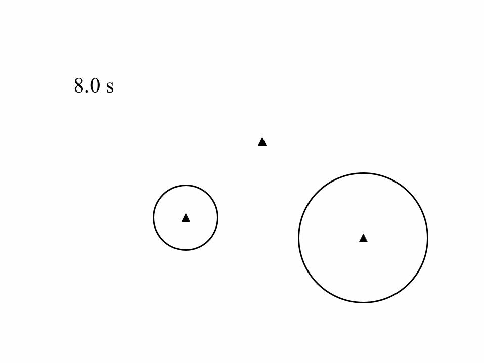
8 s 8 s

8 s 9 s 9 s

10 s

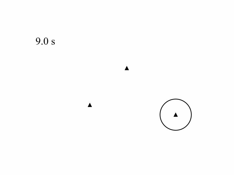
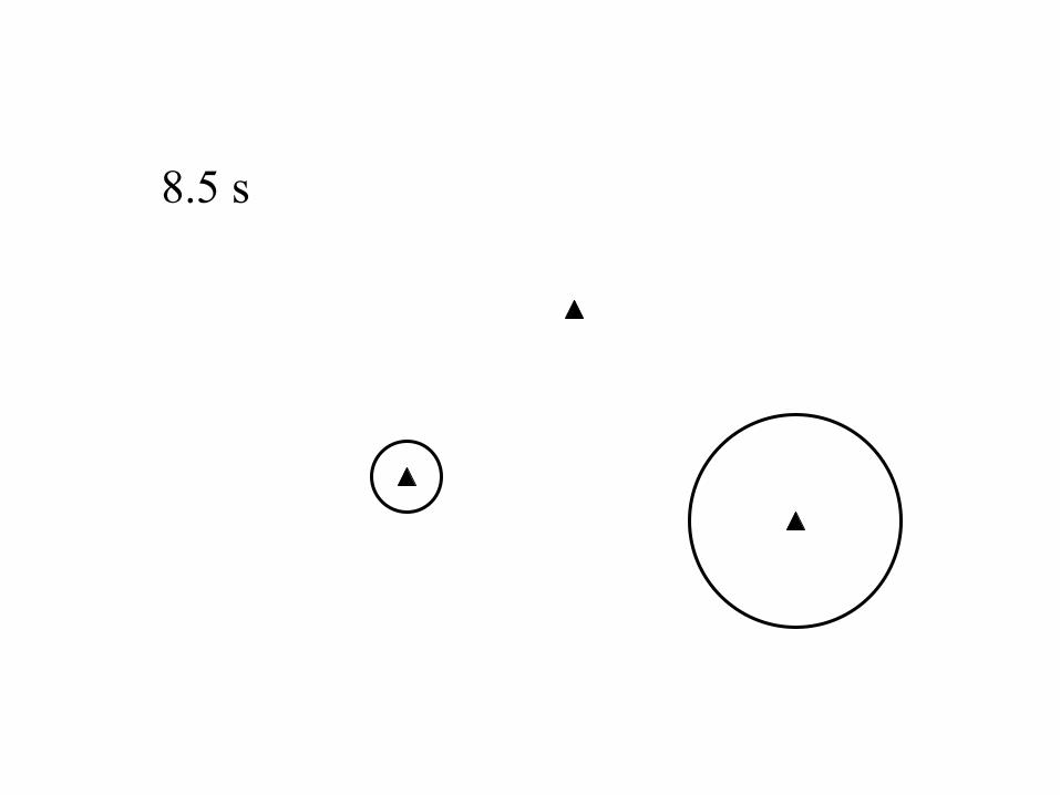
Possible event locations at 8 s (red circles)

Distance wave travels in 1 second

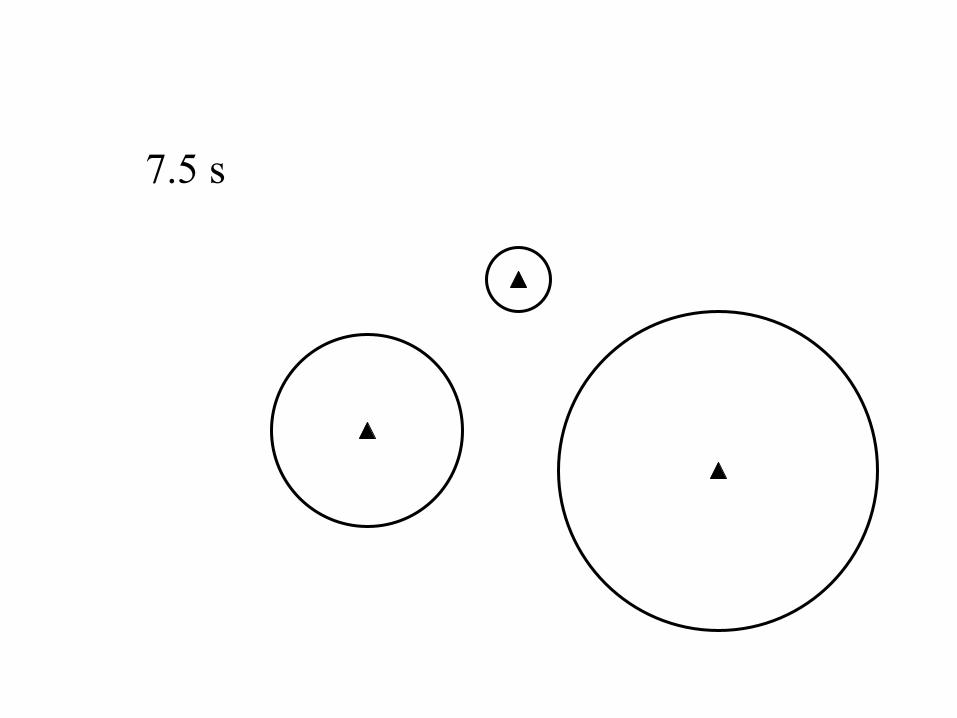
Possible event locations at 7 s (red circles)

7 s

7 7

8 8

9 9 10

Distance wave travels in 1 second

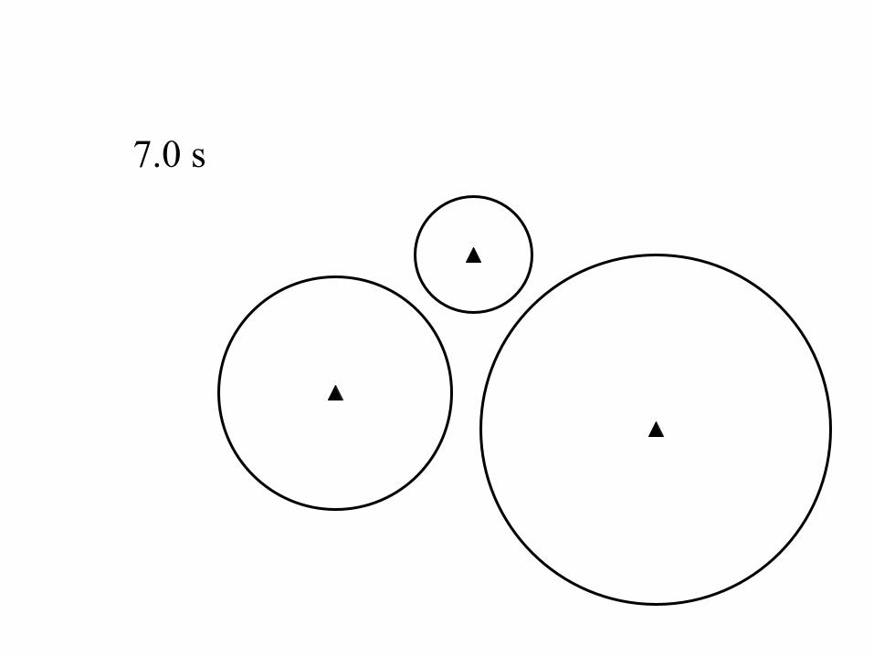
Possible event locations at 6.5 s (red circles)

6.5 s

6.5 s 6.5 s 8 s

9 s 10 s

Best-fitting location

Distance wave travels in 1 second

Time reversal and back-projection

Possible event locations at 7 s (red circles)

7 s

7 7

8 8

9 9 10

Distance wave travels in 1 second

10.0 s

9.5 s

9.0 s

8.5 s

8.0 s

7.5 s

7.0 s

6.5 s

6.5 s

Exact fit from three stations

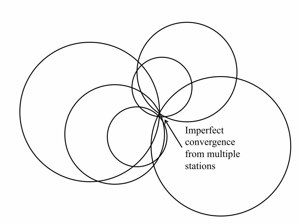
Imperfect convergence from multiple stations

Image of "best" location

Source-receiver reciprocity

Both have same ray path and travel time

Source

Source

Receiver

Receiver

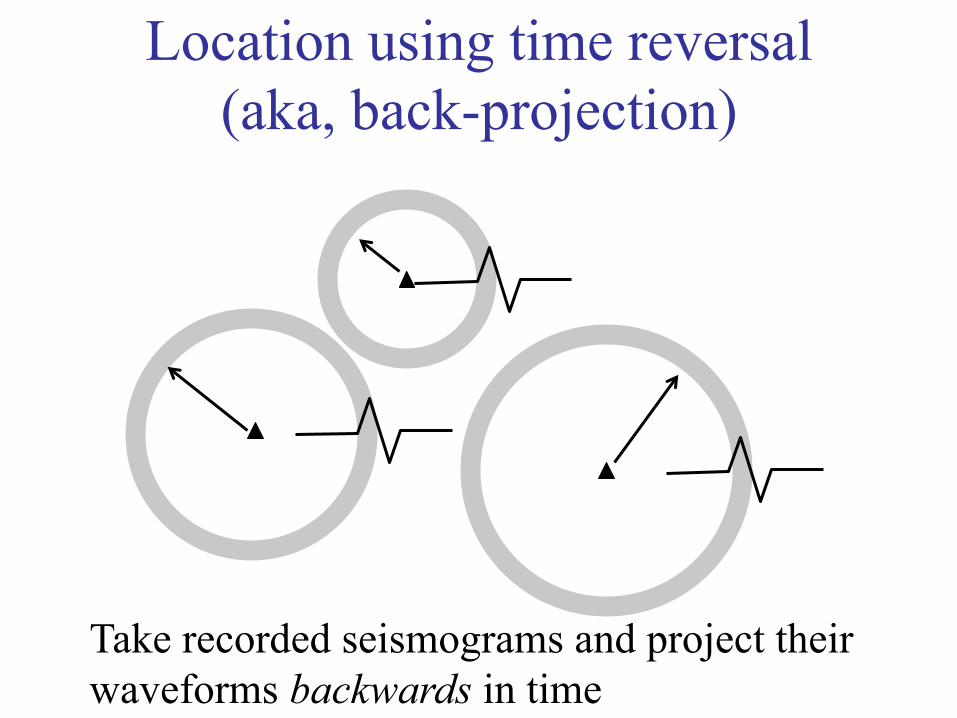
Location using time reversal (aka, back-projection)

Take recorded seismograms and project their waveforms backwards in time

At the source origin time, their waves will constructively interfere at the source location:

So what? We already have better ways to locate earthquakes.

Finite source inversion

• Assume specific fault geometry & gridding

• Compute Green’s function (synthetic seismogram) from each grid point to each station

• Set up and solve inverse problem for time-space slip model that predicts observed seismograms

• Only stable at relatively long periods

data

Slip model

First-arrival locations define the earthquake hypocenter, where the rupture starts. The seismic radiation from the rest of the rupture arrives later in the seismogram.

? ? ?

Fault slip

Hypocenter

Later parts of rupture

First arrival comes from hypocenter

Later energy comes from later parts of rupture

Back-projection potentially can locate sources of energy throughout the rupture

Migration in Reflection Seismology

Complete image is sum of individual point scatterers

* * * *

* * * * * *

Assume point scatterers

For each pixel in image, sum values from each trace at time of predicted source-to-scatterer-to-receiver travel time

“Exploding reflector” model

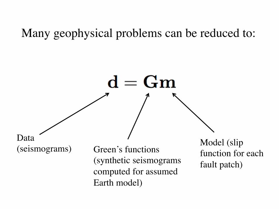
Data (seismograms) Green’s functions

(synthetic seismograms computed for assumed Earth model)

Model (slip function for each fault patch)

Many geophysical problems can be reduced to:

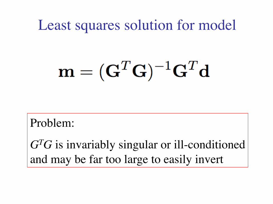
Least squares solution for model

Problem:

GTG is invariably singular or ill-conditioned and may be far too large to easily invert

A practical inversion approach

Ignore the troublesome inverse term, i.e., set it to one

Then an estimate for the model is easily obtained

GT is called the adjoint operator

Can we really get away with this?

Jon Claerbout

Inverse theory is the fine art of dividing by zero (inverting a singular matrix).

…. in practice the adjoint sometimes does a better job than the inverse! This is because the adjoint operator tolerates imperfections in the data and does not demand that the data provide full information.

With large real data sets, the answer is yes surprisingly often.

Back-projection to image earthquake rupture

2004 Sumatra-Andaman earthquake

Japanese Hi-Net array of 700 stations

Miaki Ishii

Source Imaging Using Back-projection

Assume grid of possible source locations

Stack along predicted P-wave travel time curves

Problem: Incoherent stacking from time shifts from 3-D structure

Unmodeled 3-D velocity perturbations cause time shifts in wavefront

Sumatra earthquake P-waves

Aligned on theoretical (iasp91) P-wave travel times

Migration in Reflection Seismology

*

Problem:

Time shifts from 3-D structure can destroy stack coherence

Solution:

Statics corrections (station terms)

slow slow fast

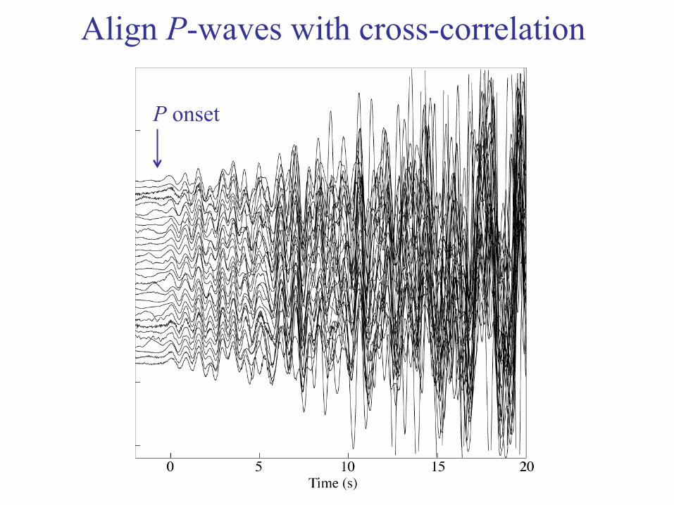
Align P-waves with cross-correlation

P onset

Method forces coherent stack at hypocenter

Cross-correlation times correct for perturbations along each hypocenter-station ray path

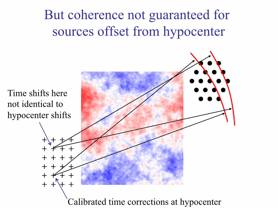
But coherence not guaranteed for sources offset from hypocenter

Calibrated time corrections at hypocenter

Time shifts here not identical to hypocenter shifts

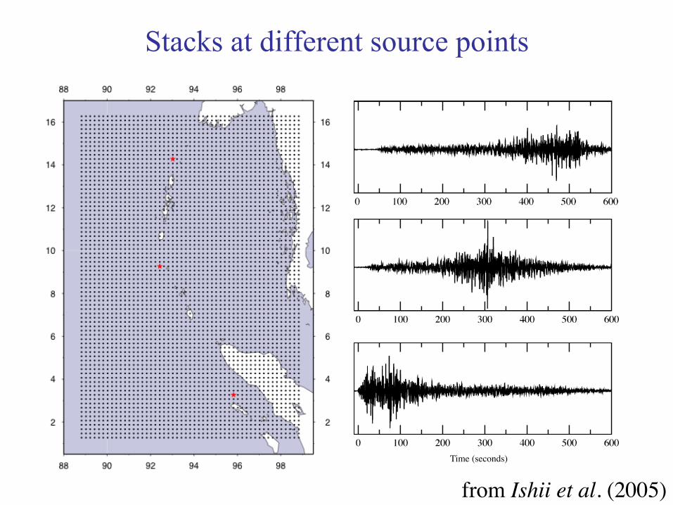
Stacks at different source points

Time (seconds)

from Ishii et al. (2005)

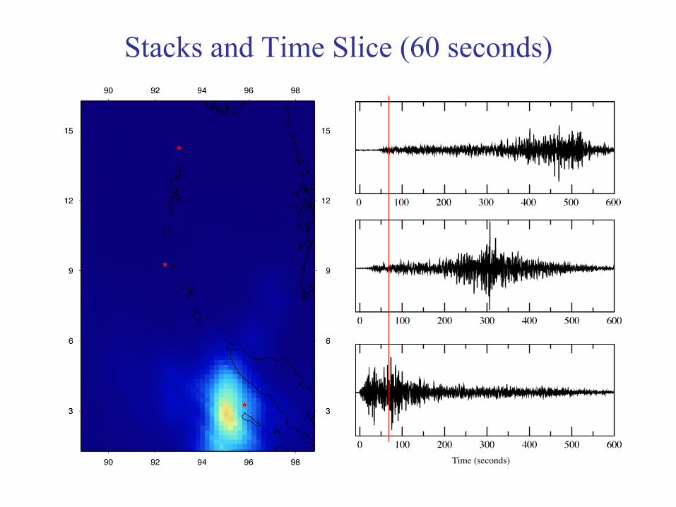
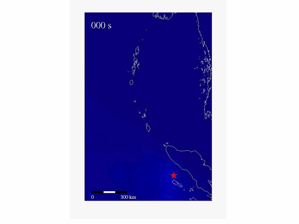
Stacks and Time Slice (60 seconds)

Time (seconds)

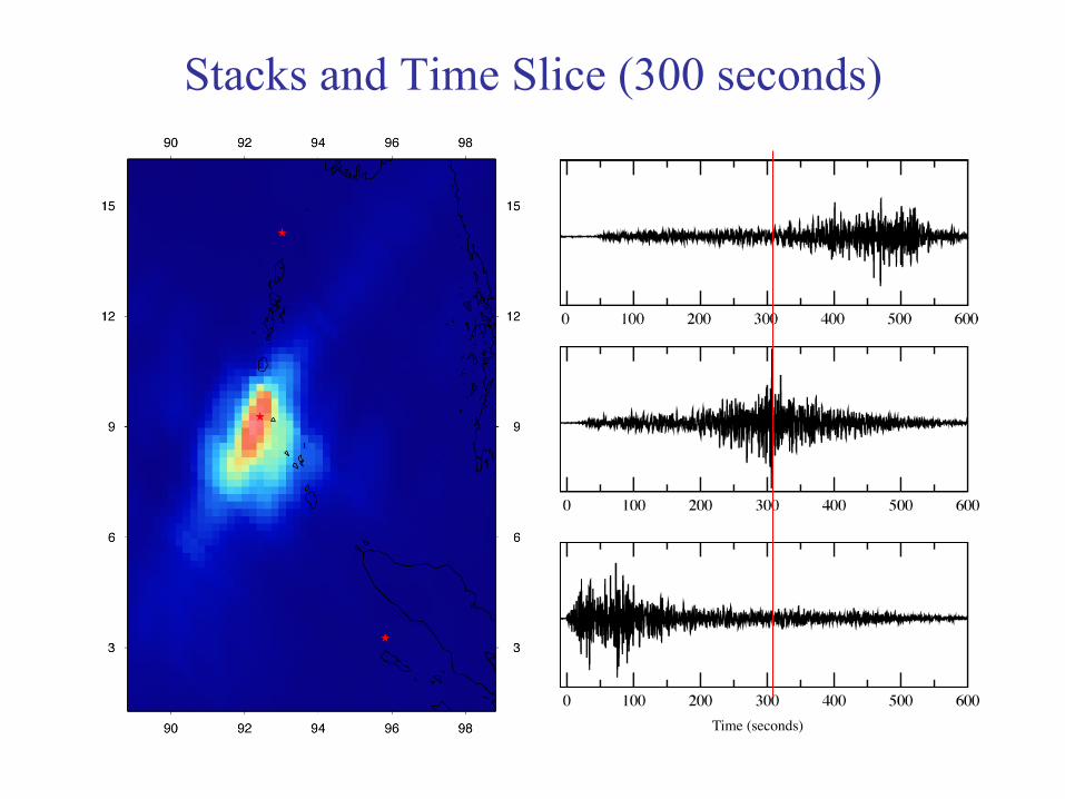
Stacks and Time Slice (300 seconds)

Time (seconds)

Short-period radiation from Hi-net backprojection (Ishii et al., 2005)

Harvard multiple CMT solution (Tsai et al., 2005)

Technical Note:

Back-projection is a form of time reversal where we approximate the P-wave Green’s function as a time-shifted delta function.

This works well for teleseismic arrivals between 30° and 90° where pulses are simple and amplitude variations are small.

Full waveform time reversal

Seismograms from 165 global stations sent back in time using normal mode Green’s functions (> 150 s period). Image is mainly of surface waves.

from Larmat et al. (2006)

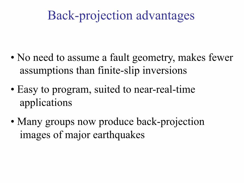
Back-projection advantages

• No need to assume a fault geometry, makes fewer assumptions than finite-slip inversions

• Easy to program, suited to near-real-time applications

• Many groups now produce back-projection images of major earthquakes

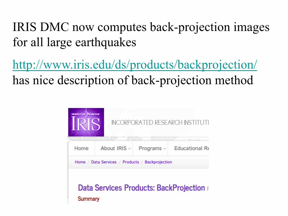
IRIS DMC now computes back-projection images for all large earthquakes

http://www.iris.edu/ds/products/backprojection/ has nice description of back-projection method

Back-projection cautionary note

Making images is easy!

The real problem is figuring out what parts of the images are reliable.

Details and Complications

• Maps high-frequency radiation, not slip (complementary to finite slip inversions)

• Subject to ‘sweeping’ artifacts

• Works best using regional arrays, not full global network, not clear why

• In principle, could be improved using aftershock calibration events, but Ishii et al. follow up study did not show much improvement

High-frequency radiation imaged by back-projection does not necessarily come from the fault patches with the largest slip

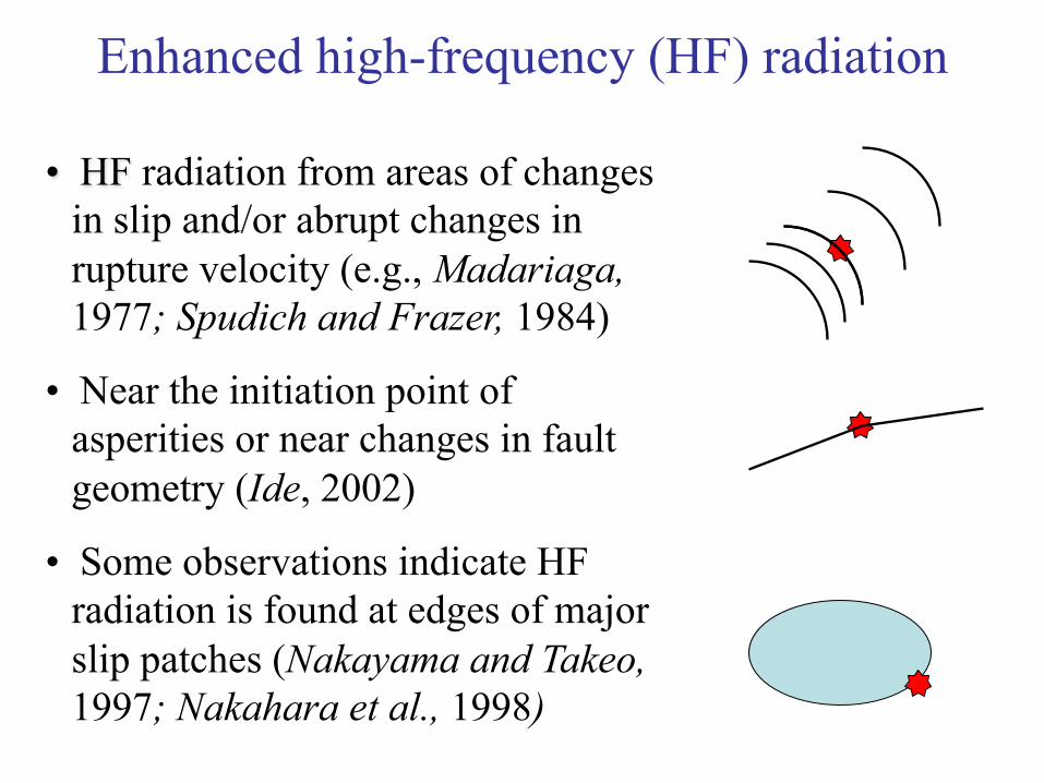
Enhanced high-frequency (HF) radiation

• HF radiation from areas of changes in slip and/or abrupt changes in rupture velocity (e.g., Madariaga, 1977; Spudich and Frazer, 1984)

• Near the initiation point of asperities or near changes in fault geometry (Ide, 2002)

• Some observations indicate HF radiation is found at edges of major slip patches (Nakayama and Takeo, 1997; Nakahara et al., 1998)

Distance ( km )

Dis

tanc

e ( k

m )

Left mouse button picks points, Right mouse button picks last point.

−100 −50 0 50 100

−50

0

50

0.5

1

1.5

Distance ( km )

Dis

tanc

e ( k

m )

−100 −50 0 50 100

−50

0

50

10

20

30

40

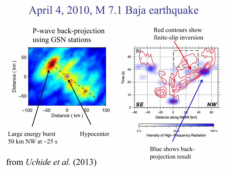
April 4, 2010, M 7.1 Baja earthquake

P-wave back-projection using GSN stations

Hypocenter Large energy burst 50 km NW at ~25 s

from Uchide et al. (2013)

Red contours show finite-slip inversion

Blue shows back-projection result

“Sweeping” or “Swimming” artifacts often seen in back-projection animations. Do not confuse these with rupture propagation.

Radiator imaged at t = 0 s

Image at t = 1 s

Image at t = 2 s

Image at t = 3 s

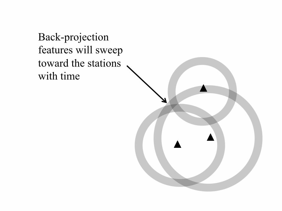
Back-projection features will sweep toward the stations with time

Sweeping artifacts

Back-projection of 2010 Chile earthquake by Kiser and Ishii

Hi-Net USArray

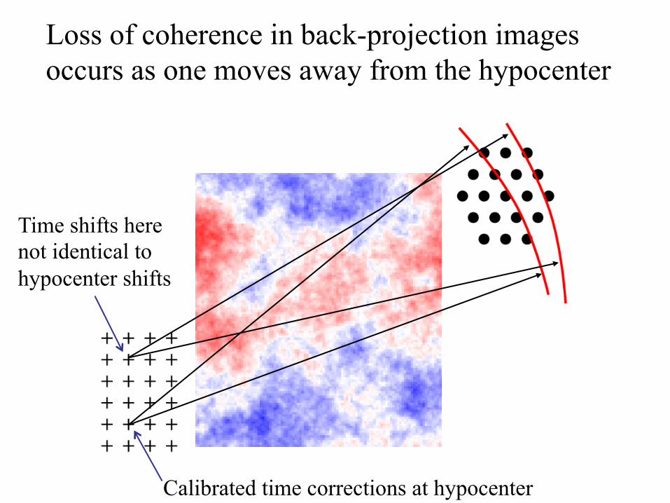
Loss of coherence in back-projection images occurs as one moves away from the hypocenter

Calibrated time corrections at hypocenter

Time shifts here not identical to hypocenter shifts

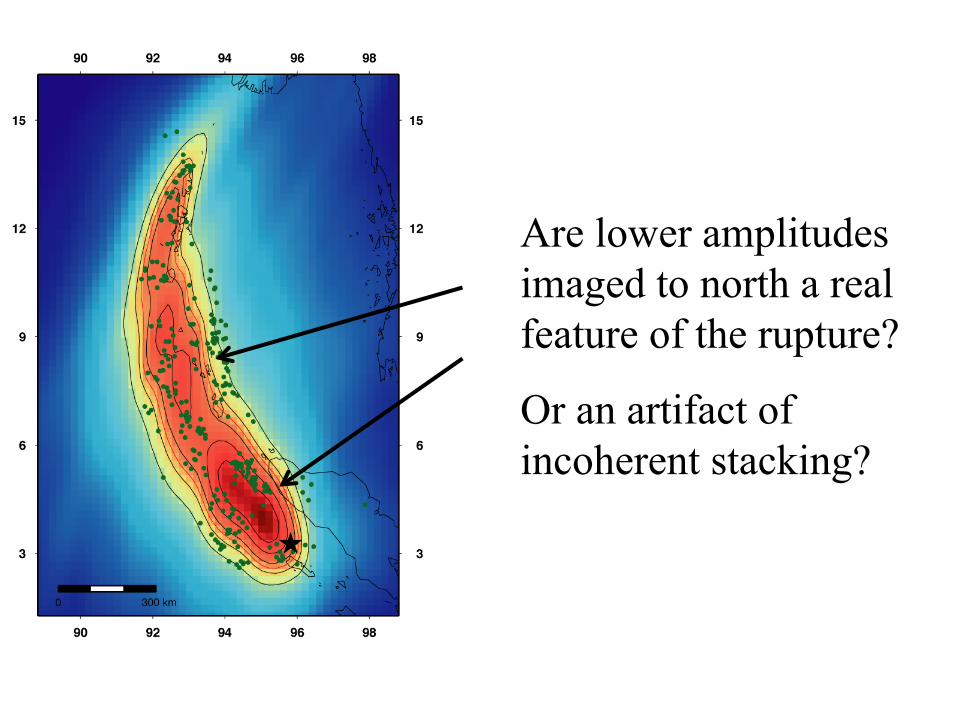
Are lower amplitudes imaged to north a real feature of the rupture?

Or an artifact of incoherent stacking?

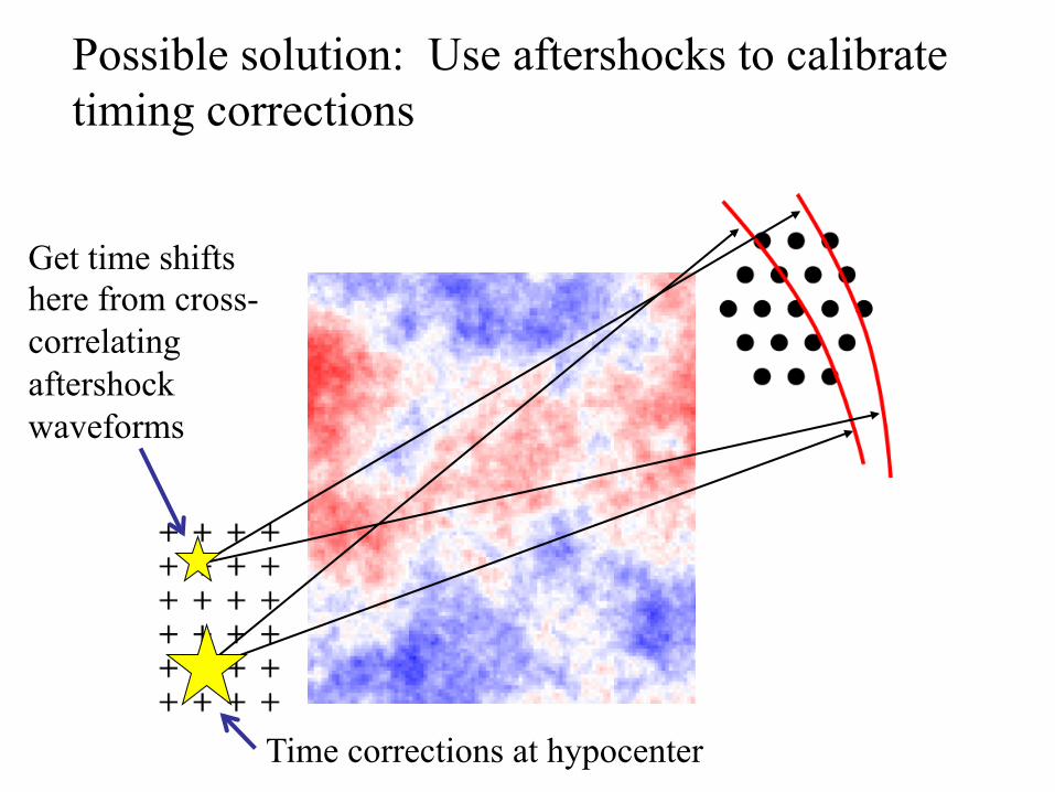
Possible solution: Use aftershocks to calibrate timing corrections

Time corrections at hypocenter

Get time shifts here from cross-correlating aftershock waveforms

Aftershock calibration for back-projection

from Ishii et al. (2007)

Time corrected using mainshock hypocenter

Time corrected using 46 aftershocks (black dots)

In theory, back-projection resolution kernels are smaller (i.e., better resolution) for:

Higher frequencies (but incoherence limits how high one can go)

Better azimuthal station coverage (but not always true in practice)

Theoretical Resolution Kernels

Global station distribution yields very tight kernel, should have much better resolution.

Regional array (Hi-Net, USArray) yields broader kernel, should have poorer resolution. But in practice usually works better! Why?

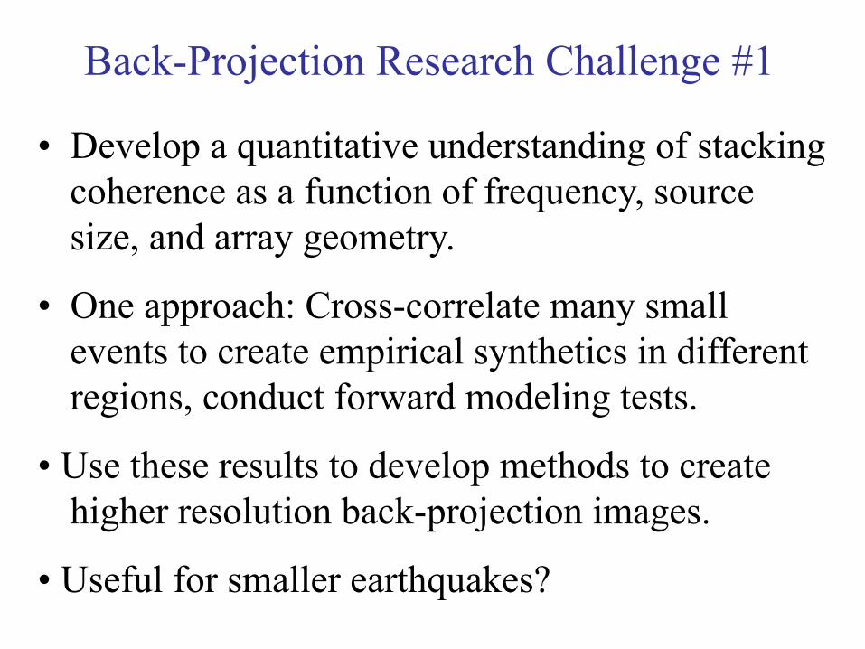
Back-Projection Research Challenge #1

• Develop a quantitative understanding of stacking coherence as a function of frequency, source size, and array geometry.

• One approach: Cross-correlate many small events to create empirical synthetics in different regions, conduct forward modeling tests.

• Use these results to develop methods to create higher resolution back-projection images.

• Useful for smaller earthquakes?

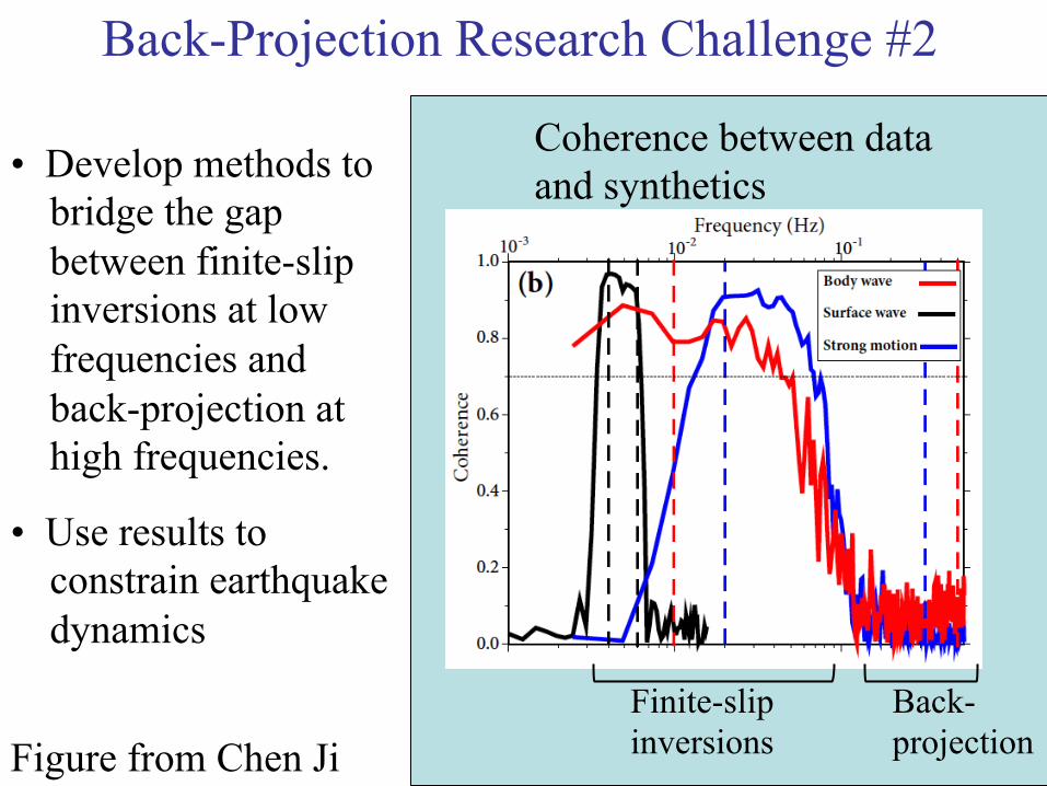
Back-Projection Research Challenge #2

• Develop methods to bridge the gap between finite-slip inversions at low frequencies and back-projection at high frequencies.

• Use results to constrain earthquake dynamics

Coherence between data and synthetics

Finite-slip inversions

Back-projection Figure from Chen Ji

Your Immediate Task: Computer Exercise 1

• Described at end of notes. Get needed files from: http://igppweb.ucsd.edu/~shearer/SCECERI/

• Data are provided. You must write your own program (e.g., F90, C, or Python) to back-project and image tremor sources.