Background-error correlation modelling in variational ...€¦ · Applications of data assimilation in oceanography Providing initial conditions for climate forecasts. Monthly, seasonal,

.

......

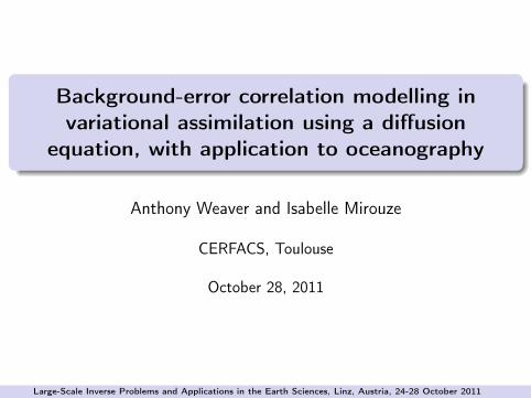
Background-error correlation modelling invariational assimilation using a diffusion

equation, with application to oceanography

Anthony Weaver and Isabelle Mirouze

CERFACS, Toulouse

October 28, 2011

Large-Scale Inverse Problems and Applications in the Earth Sciences, Linz, Austria, 24-28 October 2011

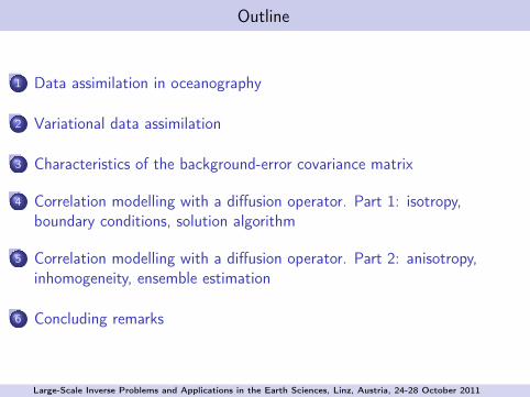
Outline

...1 Data assimilation in oceanography

...2 Variational data assimilation

...3 Characteristics of the background-error covariance matrix

...4 Correlation modelling with a diffusion operator. Part 1: isotropy,boundary conditions, solution algorithm

...5 Correlation modelling with a diffusion operator. Part 2: anisotropy,inhomogeneity, ensemble estimation

...6 Concluding remarks


Outline








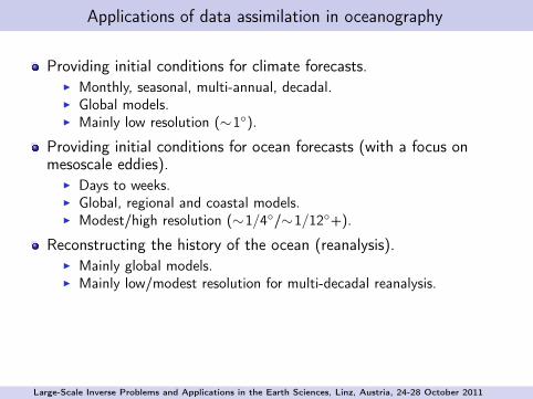
Applications of data assimilation in oceanography

Providing initial conditions for climate forecasts.▶ Monthly, seasonal, multi-annual, decadal.▶ Global models.▶ Mainly low resolution (∼1◦).

Providing initial conditions for ocean forecasts (with a focus onmesoscale eddies).

▶ Days to weeks.▶ Global, regional and coastal models.▶ Modest/high resolution (∼1/4◦/∼1/12◦+).

Reconstructing the history of the ocean (reanalysis).▶ Mainly global models.▶ Mainly low/modest resolution for multi-decadal reanalysis.


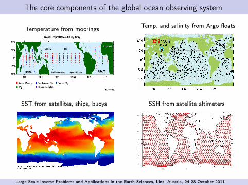
The core components of the global ocean observing system

Temperature from moorings Temp. and salinity from Argo floats

SST from satellites, ships, buoys SSH from satellite altimeters


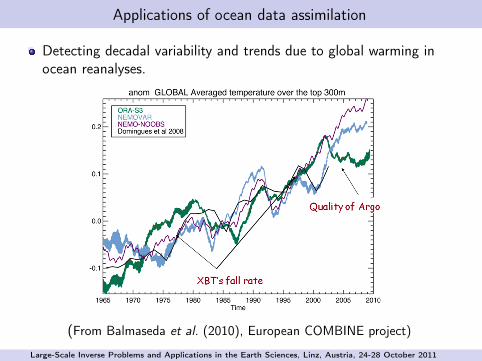
Applications of ocean data assimilation

Detecting decadal variability and trends due to global warming inocean reanalyses.

(From Balmaseda et al. (2010), European COMBINE project)


Outline








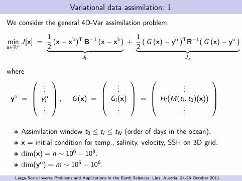
Variational data assimilation: I

We consider the general 4D-Var assimilation problem:

minx∈Rn

J[x] =12(x − xb)T B−1 (x − xb)︸︷︷︸

Jb

+12(G (x)− yo )TR−1(G (x)− yo )︸︷︷︸

Jo

where

yo =

...

yoi...

, G (x) =

...

Gi (x)...

=

...

Hi (M(ti , t0)(x))...

Assimilation window t0 ≤ ti ≤ tN (order of days in the ocean).x = initial condition for temp., salinity, velocity, SSH on 3D grid.dim(x) = n ∼ 106 − 108.dim(yo) = m ∼ 105 − 106.


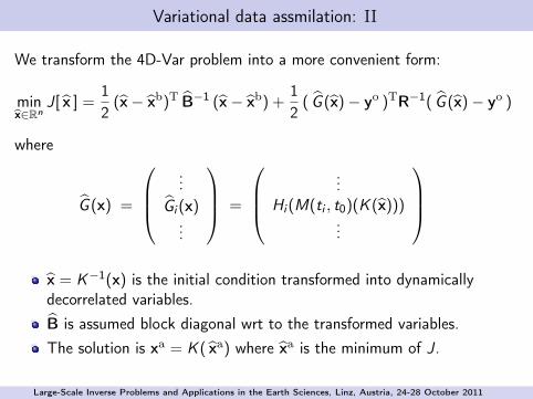
Variational data assmilation: II

We transform the 4D-Var problem into a more convenient form:

minx∈Rn

J[ x ] =12(x − xb)T B−1 (x − xb) +

12( G (x)− yo )TR−1( G (x)− yo )

where

G (x) =

...

Gi (x)...

=

...

Hi (M(ti , t0)(K (x)))...

x = K−1(x) is the initial condition transformed into dynamicallydecorrelated variables.B is assumed block diagonal wrt to the transformed variables.The solution is xa = K ( xa) where xa is the minimum of J.


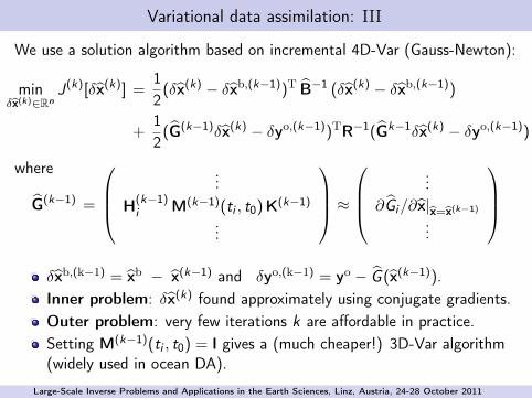
Variational data assimilation: III

We use a solution algorithm based on incremental 4D-Var (Gauss-Newton):

minδx(k)∈Rn

J(k)[δx(k)] =12(δx(k) − δxb,(k−1))T B−1 (δx(k) − δxb,(k−1))

+12(G(k−1)δx(k) − δyo,(k−1))TR−1(Gk−1δx(k) − δyo,(k−1))

where

G(k−1) =

...

H(k−1)i M(k−1)(ti , t0)K(k−1)

...

≈

...

∂Gi/∂x|x=x(k−1)

...

δxb,(k−1) = xb − x(k−1) and δyo,(k−1) = yo − G (x(k−1)).Inner problem: δx(k) found approximately using conjugate gradients.Outer problem: very few iterations k are affordable in practice.Setting M(k−1)(ti , t0) = I gives a (much cheaper!) 3D-Var algorithm(widely used in ocean DA).


Outline








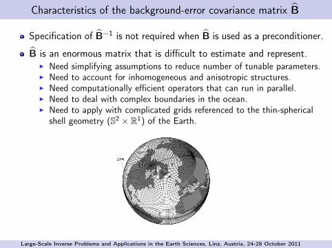
Characteristics of the background-error covariance matrix B

Specification of B−1 is not required when B is used as a preconditioner.

B is an enormous matrix that is difficult to estimate and represent.▶ Need simplifying assumptions to reduce number of tunable parameters.▶ Need to account for inhomogeneous and anisotropic structures.▶ Need computationally efficient operators that can run in parallel.▶ Need to deal with complex boundaries in the ocean.▶ Need to apply with complicated grids referenced to the thin-spherical

shell geometry (S2 × R1) of the Earth.


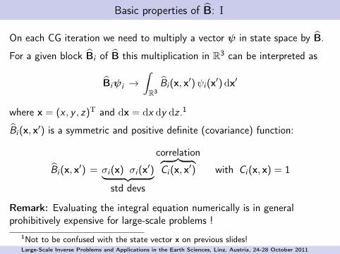
Basic properties of B: I

On each CG iteration we need to multiply a vector ψ in state space by B.

For a given block Bi of B this multiplication in R3 can be interpreted as

Biψi →∫R3

Bi (x, x′)ψi (x′) dx′

where x = (x , y , z)T and dx = dx dy dz .1

Bi (x, x′) is a symmetric and positive definite (covariance) function:

Bi (x, x′) = σi (x) σi (x′)︸︷︷︸std devs

correlation︷︸︸︷Ci (x, x′) with Ci (x, x) = 1

Remark: Evaluating the integral equation numerically is in generalprohibitively expensive for large-scale problems !

1Not to be confused with the state vector x on previous slides!Large-Scale Inverse Problems and Applications in the Earth Sciences, Linz, Austria, 24-28 October 2011

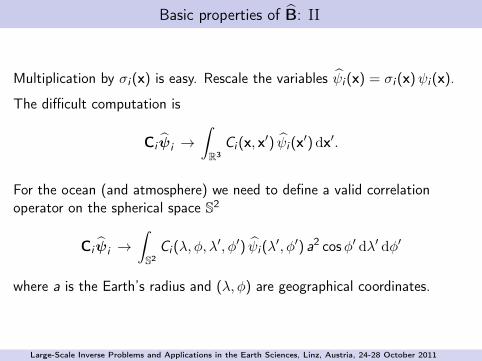
Basic properties of B: II

Multiplication by σi (x) is easy. Rescale the variables ψi (x) = σi (x)ψi (x).

The difficult computation is

Ci ψi →∫R3

Ci (x, x′) ψi (x′) dx′.

For the ocean (and atmosphere) we need to define a valid correlationoperator on the spherical space S2

Ci ψi →∫S2

Ci (λ, ϕ, λ′, ϕ′) ψi (λ

′, ϕ′) a2 cosϕ′ dλ′ dϕ′

where a is the Earth’s radius and (λ, ϕ) are geographical coordinates.


Outline








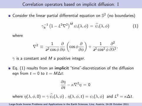
Correlation operators based on implicit diffusion: I

Consider the linear partial differential equation on S2 (no boundaries)

γ−1h

(1 − L2∇2)M ψi (λ, ϕ) = ψi (λ, ϕ) (1)

where

∇2 ≡ 1a2 cosϕ

∂

∂ϕ

(cosϕ

∂

∂ϕ

)+

1a2 cos2 ϕ

∂2

∂λ2 ,

γ is a constant and M a positive integer.

Eq. (1) results from an implicit “time”-discretization of the diffusioneqn from t = 0 to t = M∆t:

∂η

∂t− κ∇2η = 0

where η(λ, ϕ, 0) = γ ψi (λ, ϕ) , η(λ, ϕ, t) = ψi (λ, ϕ) and L2 = κ∆t.


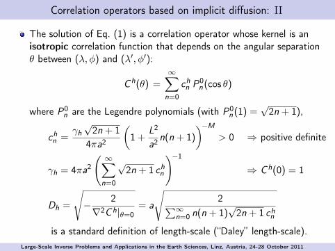
Correlation operators based on implicit diffusion: II

The solution of Eq. (1) is a correlation operator whose kernel is anisotropic correlation function that depends on the angular separationθ between (λ, ϕ) and (λ′, ϕ′):

C h(θ) =∞∑

n=0

chn P0

n(cos θ)

where P0n are the Legendre polynomials (with P0

n(1) =√

2n + 1),

chn =

γh√

2n + 14πa2

(1 +

L2

a2 n(n + 1))−M

> 0 ⇒ positive definite

γh = 4πa2

( ∞∑n=0

√2n + 1 ch

n

)−1

⇒ Ch(0) = 1

Dh =

√− 2∇2Ch|θ=0

= a

√2∑∞

n=0 n(n + 1)√

2n + 1 chn

is a standard definition of length-scale (“Daley” length-scale).Large-Scale Inverse Problems and Applications in the Earth Sciences, Linz, Austria, 24-28 October 2011

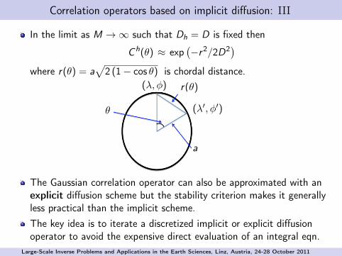
Correlation operators based on implicit diffusion: III

In the limit as M → ∞ such that Dh = D is fixed then

Ch(θ) ≈ exp(−r2/2D2)

where r(θ) = a√

2 (1 − cos θ) is chordal distance.(λ, ϕ)

(λ′, ϕ′)θ

r(θ)

a

The Gaussian correlation operator can also be approximated with anexplicit diffusion scheme but the stability criterion makes it generallyless practical than the implicit scheme.The key idea is to iterate a discretized implicit or explicit diffusionoperator to avoid the expensive direct evaluation of an integral eqn.


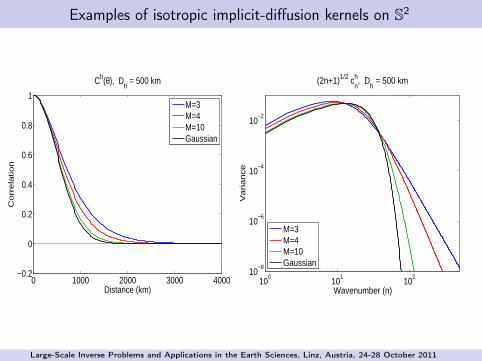
Examples of isotropic implicit-diffusion kernels on S2

0 1000 2000 3000 4000−0.2

0

0.2

0.4

0.6

0.8

1

Distance (km)

Co

rre

latio

n

Ch(θ), Dh = 500 km

M=3M=4M=10Gaussian

100

101

102

10−8

10−6

10−4

10−2

Wavenumber (n)

Va

ria

nce

(2n+1)1/2 chn, D

h = 500 km

M=3M=4M=10Gaussian


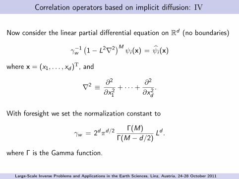
Correlation operators based on implicit diffusion: IV

Now consider the linear partial differential equation on Rd (no boundaries)

γ−1w(1 − L2∇2)M ψi (x) = ψi (x)

where x = (x1, . . . , xd)T, and

∇2 ≡ ∂2

∂x21+ · · ·+ ∂2

∂x2d.

With foresight we set the normalization constant to

γw = 2dπd/2 Γ(M)

Γ(M − d/2)Ld .

where Γ is the Gamma function.


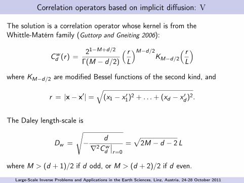
Correlation operators based on implicit diffusion: V

The solution is a correlation operator whose kernel is from theWhittle-Matérn family (Guttorp and Gneiting 2006):

Cwd (r) =

21−M+d/2

Γ(M − d/2)

( rL

)M−d/2KM−d/2

( rL

)where KM−d/2 are modified Bessel functions of the second kind, and

r = |x − x′| =√

(x1 − x ′1)

2 + . . .+ (xd − x ′d )

2.

The Daley length-scale is

Dw =

√− d∇2Cw

d

∣∣r=0

=√

2M − d − 2 L

where M > (d + 1)/2 if d odd, or M > (d + 2)/2 if d even.


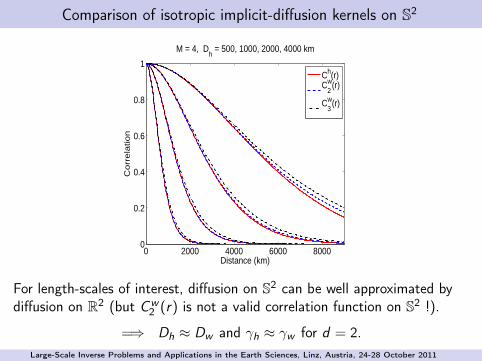
Comparison of isotropic implicit-diffusion kernels on S2

0 2000 4000 6000 80000

0.2

0.4

0.6

0.8

1

Distance (km)

Co

rre

latio

n

M = 4, Dh = 500, 1000, 2000, 4000 km

Ch(r)Cw

2(r)

Cw3

(r)

For length-scales of interest, diffusion on S2 can be well approximated bydiffusion on R2 (but Cw

2 (r) is not a valid correlation function on S2 !).

=⇒ Dh ≈ Dw and γh ≈ γw for d = 2.Large-Scale Inverse Problems and Applications in the Earth Sciences, Linz, Austria, 24-28 October 2011

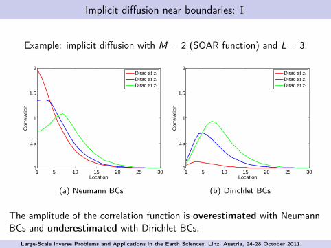
Implicit diffusion near boundaries: I

Example: implicit diffusion with M = 2 (SOAR function) and L = 3.

1 5 10 15 20 25 300

0.5

1

1.5

2

Location

Cor

rela

tion

Dirac at z1

Dirac at z4

Dirac at z7

(a) Neumann BCs

1 5 10 15 20 25 300

0.5

1

1.5

2

LocationC

orre

latio

n

Dirac at z1

Dirac at z4

Dirac at z7

(b) Dirichlet BCs

The amplitude of the correlation function is overestimated with NeumannBCs and underestimated with Dirichlet BCs.


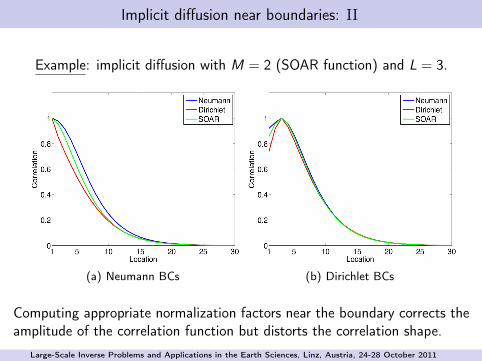
Implicit diffusion near boundaries: II


(a) Neumann BCs (b) Dirichlet BCs

Computing appropriate normalization factors near the boundary corrects theamplitude of the correlation function but distorts the correlation shape.


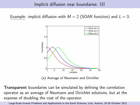
Implicit diffusion near boundaries: III


1 5 10 15 20 25 300

0.5

1

1.5

2

Location

Cor

rela

tion

Dirac at z1

Dirac at z4

Dirac at z7

(a) Average of Neumann and Dirichlet

Transparent boundaries can be simulated by defining the correlationoperator as an average of Neumann and Dirichlet solutions, but at theexpense of doubling the cost of the operator.


Solving the implicit diffusion equation: I

The implicit diffusion equation requires the solution of a large linearsystem

AMψ = (I − D)M ψ = ψ (1)

where D → ∇ · L2∇ with L = L(x) to account for geographicallyvarying length-scales.

Let L−1 = A so that the (unnormalized) solution can be written as

ψ = LMψ.

Direct methods for solving Eq. (1) are not practical in 2D or 3D, butcan be applied in 1D (e.g., using Cholesky factorization).


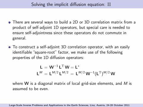
Solving the implicit diffusion equation: II

There are several ways to build a 2D or 3D correlation matrix from aproduct of self-adjoint 1D operators, but special care is needed toensure self-adjointness since these operators do not commute ingeneral.

To construct a self-adjoint 3D correlation operator, with an easilyidentifiable “square-root” factor, we make use of the followingproperties of the 1D diffusion operators:

L = W−1 LT W = L∗

LM = LM/2 LM/2 = LM/2 W−1(LT)M/2 W

where W is a diagonal matrix of local grid-size elements, and M isassumed to be even.


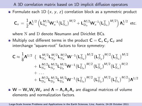
A 3D correlation matrix based on 1D implicit diffusion operators

Formulate each 1D (x , y , z) correlation block as a symmetric product

Cx =12Λ

1/2x

(LM/2

NxW−1

x(LT

Nx

)M/2+ LM/2

DxW−1

x(LT

Dx

)M/2)Λ

1/2x etc.

where N and D denote Neumann and Dirichlet BCs.Multiply out different terms in the product C = Cx Cy Cz andinterchange “square-root” factors to force symmetry:

C ≈ 18Λ1/2 { LM/2

NxLM/2

NyLM/2

NzW−1(LT

Nz

)M/2(LT

Ny )M/2(

LTNx

)M/2

+ LM/2Nx

LM/2Ny

LM/2Dz

W−1(LTDz

)M/2(LT

Ny )M/2(

LTNx

)M/2

+ . . .

+ LM/2Dx

LM/2Dy

LM/2Dz

W−1(LTDz

)M/2(LT

Dy )M/2(

LTDx

)M/2}Λ1/2

W = WxWyWz and Λ = ΛxΛyΛz are diagonal matrices of volumeelements and normalization factors.


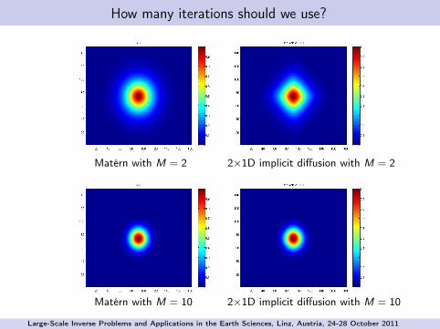
How many iterations should we use?

Matérn with M = 2 2×1D implicit diffusion with M = 2

Matérn with M = 10 2×1D implicit diffusion with M = 10


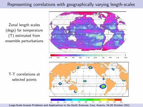
Representing correlations with geographically varying length-scales

Zonal length scales(degs) for temperature

(T) estimated fromensemble perturbations

T-T correlations atselected points


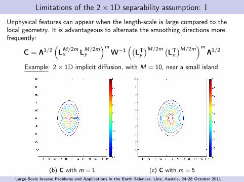
Limitations of the 2 × 1D separability assumption: I

Unphysical features can appear when the length-scale is large compared to thelocal geometry. It is advantageous to alternate the smoothing directions morefrequently:

C = Λ1/2(LM/2m

x LM/2my

)mW−1

((LT

y)M/2m (LT

x)M/2m

)mΛ1/2

Example: 2 × 1D implicit diffusion, with M = 10, near a small island.

(b) C with m = 1 (c) C with m = 5Large-Scale Inverse Problems and Applications in the Earth Sciences, Linz, Austria, 24-28 October 2011

Limitations of the 2 × 1D separability assumption: II

SST bias increments obtained with a 2 × 1D implicit diffusion: M = 12, m = 1.

(Courtesy of James While, Met Office)Large-Scale Inverse Problems and Applications in the Earth Sciences, Linz, Austria, 24-28 October 2011

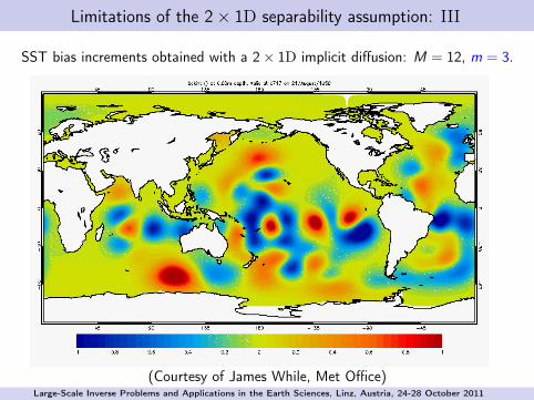
Limitations of the 2 × 1D separability assumption: III

SST bias increments obtained with a 2 × 1D implicit diffusion: M = 12, m = 3.

(Courtesy of James While, Met Office)Large-Scale Inverse Problems and Applications in the Earth Sciences, Linz, Austria, 24-28 October 2011

Outline








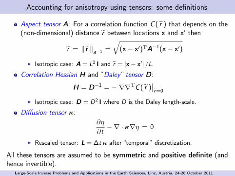
Accounting for anisotropy using tensors: some definitions

Aspect tensor A: For a correlation function C ( r ) that depends on the(non-dimensional) distance r between locations x and x′ then

r = ∥ r ∥A−1 =

√(x − x′)TA−1(x − x′)

▶ Isotropic case: A = L2 I and r = |x − x′| /L.

Correlation Hessian H and “Daley” tensor D:

H = D−1 = − ∇∇TC ( r )∣∣r=0

▶ Isotropic case: D = D2 I where D is the Daley length-scale.

Diffusion tensor κ:∂η

∂t−∇ · κ∇η = 0

▶ Rescaled tensor: L = ∆t κ after “temporal” discretization.

All these tensors are assumed to be symmetric and positive definite (andhence invertible).


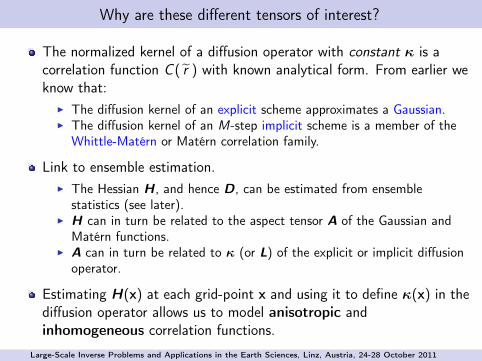
Why are these different tensors of interest?

The normalized kernel of a diffusion operator with constant κ is acorrelation function C ( r ) with known analytical form. From earlier weknow that:

▶ The diffusion kernel of an explicit scheme approximates a Gaussian.▶ The diffusion kernel of an M-step implicit scheme is a member of the

Whittle-Matérn or Matérn correlation family.

Link to ensemble estimation.▶ The Hessian H , and hence D, can be estimated from ensemble

statistics (see later).▶ H can in turn be related to the aspect tensor A of the Gaussian and

Matérn functions.▶ A can in turn be related to κ (or L) of the explicit or implicit diffusion

operator.

Estimating H(x) at each grid-point x and using it to define κ(x) in thediffusion operator allows us to model anisotropic andinhomogeneous correlation functions.


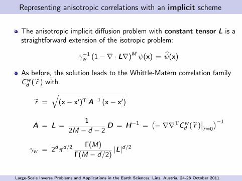
Representing anisotropic correlations with an implicit scheme

The anisotropic implicit diffusion problem with constant tensor L is astraightforward extension of the isotropic problem:

γ−1w (1 −∇ · L∇)M ψ(x) = ψ(x)

As before, the solution leads to the Whittle-Matérn correlation familyCw

d ( r ) with

r =

√(x − x′)T A−1 (x − x′)

A = L =1

2M − d − 2D = H−1 =

(− ∇∇TCw

d ( r )∣∣r=0

)−1

γw = 2dπd/2 Γ(M)

Γ(M − d/2)|L|d/2


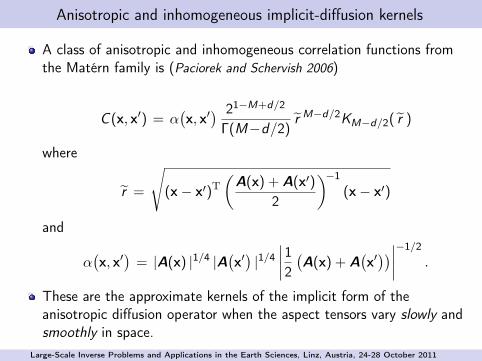
Anisotropic and inhomogeneous implicit-diffusion kernels

A class of anisotropic and inhomogeneous correlation functions fromthe Matérn family is (Paciorek and Schervish 2006)

C (x, x′) = α(x, x′

) 21−M+d/2

Γ(M−d/2)r M−d/2KM−d/2( r )

where

r =

√(x − x′)T

(A(x) + A(x′)

2

)−1

(x − x′)

and

α(x, x′

)= |A(x) |1/4 |A

(x′)|1/4

∣∣∣∣12 (A(x) + A(x′))∣∣∣∣−1/2

.

These are the approximate kernels of the implicit form of theanisotropic diffusion operator when the aspect tensors vary slowly andsmoothly in space.


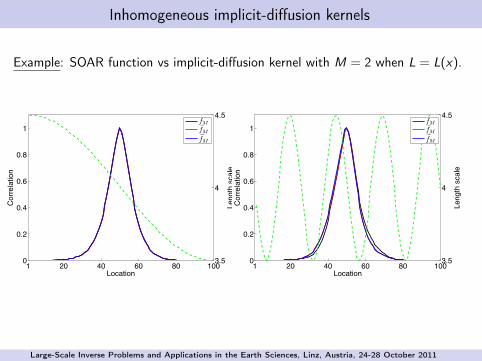
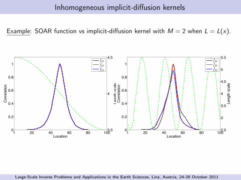
Inhomogeneous implicit-diffusion kernels

Example: SOAR function vs implicit-diffusion kernel with M = 2 when L = L(x).

1 20 40 60 80 1000

0.2

0.4

0.6

0.8

1

Cor

rela

tion

Location

3.5

4

4.5

Leng

th s

cale

fM

fM!fM

1 20 40 60 80 1000

0.2

0.4

0.6

0.8

1

Cor

rela

tion

Location

3.5

4

4.5

Leng

th s

cale

fM

fM!fM


Inhomogeneous implicit-diffusion kernels

Example: SOAR function vs implicit-diffusion kernel with M = 2 when L = L(x).

1 20 40 60 80 1000

0.2

0.4

0.6

0.8

1

Cor

rela

tion

Location

3.5

4

4.5

Leng

th s

cale

fM

fM!fM

1 20 40 60 80 1000

0.2

0.4

0.6

0.8

1

Cor

rela

tion

Location

2.5

3

3.5

4

4.5

5

5.5

Leng

th s

cale

fM

fM!fM


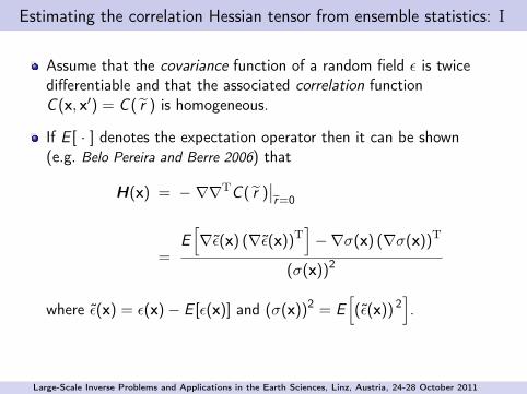
Estimating the correlation Hessian tensor from ensemble statistics: I

Assume that the covariance function of a random field ϵ is twicedifferentiable and that the associated correlation functionC (x, x′) = C ( r ) is homogeneous.

If E [ · ] denotes the expectation operator then it can be shown(e.g. Belo Pereira and Berre 2006) that

H(x) = − ∇∇TC ( r )∣∣r=0

=E[∇ϵ(x) (∇ϵ(x))T

]−∇σ(x) (∇σ(x))T

(σ(x))2

where ϵ(x) = ϵ(x)− E [ϵ(x)] and (σ(x))2 = E[(ϵ(x)) 2

].


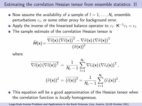
Estimating the correlation Hessian tensor from ensemble statistics: II

Now assume the availability of a sample of l = 1, . . . ,Ne ensembleperturbations εl , or some other proxy for background error.Apply the inverse of the linearized balance operator to εl : K−1εl = ϵl .The sample estimate of the correlation Hessian tensor is

H(x)=∇ϵ(x) (∇ϵ(x))T −∇σ(x) (∇σ(x))T

(σ(x))2

where

∇ϵ(x) (∇ϵ(x))T =1

Ne − 1

Ne∑l=1

∇ϵl(x) (∇ϵl (x))T ,

(σ(x))2 = (ϵ(x))2 =1

Ne − 1

Ne∑l=1

(ϵl(x))2 .

This equation will be a good approximation of the Hessian tensor whenthe correlation function is locally homogeneous.


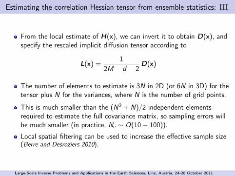
Estimating the correlation Hessian tensor from ensemble statistics: III

From the local estimate of H(x), we can invert it to obtain D(x), andspecify the rescaled implicit diffusion tensor according to

L(x) =1

2M − d − 2D(x)

The number of elements to estimate is 3N in 2D (or 6N in 3D) for thetensor plus N for the variances, where N is the number of grid points.

This is much smaller than the (N2 + N)/2 independent elementsrequired to estimate the full covariance matrix, so sampling errors willbe much smaller (in practice, Ne ∼ O(10 − 100)).

Local spatial filtering can be used to increase the effective sample size(Berre and Desroziers 2010).


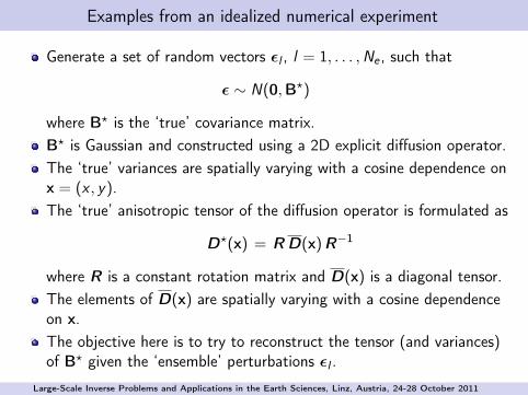
Examples from an idealized numerical experiment

Generate a set of random vectors ϵl , l = 1, . . . ,Ne , such that

ϵ ∼ N(0,B⋆)

where B⋆ is the ‘true’ covariance matrix.B⋆ is Gaussian and constructed using a 2D explicit diffusion operator.The ‘true’ variances are spatially varying with a cosine dependence onx = (x , y).The ‘true’ anisotropic tensor of the diffusion operator is formulated as

D⋆(x) = R D(x)R−1

where R is a constant rotation matrix and D(x) is a diagonal tensor.The elements of D(x) are spatially varying with a cosine dependenceon x.The objective here is to try to reconstruct the tensor (and variances)of B⋆ given the ‘ensemble’ perturbations ϵl .


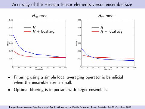
Accuracy of the Hessian tensor elements versus ensemble size

10 20 30 40 50 60 70 80 90 1000

0.01

0.02

0.03

0.04

0.05

0.06

Members

Rm

se

10 20 30 40 50 60 70 80 90 1000

0.01

0.02

0.03

0.04

0.05

0.06

Members

Rm

se

Hxx rmse Hxy rmse

—— H—— H + local avg

—— H—— H + local avg

• Filtering using a simple local averaging operator is beneficialwhen the ensemble size is small.

• Optimal filtering is important with larger ensembles.


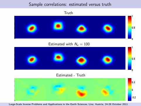
Sample correlations: estimated versus truth

Truth

Estimated with Ne = 100

Estimated - Truth


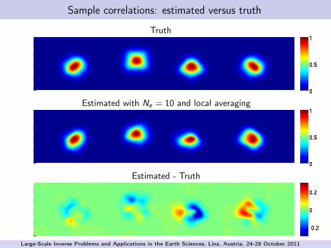
Sample correlations: estimated versus truth

Truth

Estimated with Ne = 10 and local averaging

Estimated - Truth


Outline








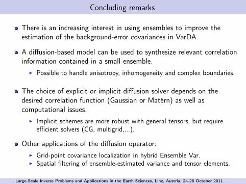
Concluding remarks

There is an increasing interest in using ensembles to improve theestimation of the background-error covariances in VarDA.

A diffusion-based model can be used to synthesize relevant correlationinformation contained in a small ensemble.

▶ Possible to handle anisotropy, inhomogeneity and complex boundaries.

The choice of explicit or implicit diffusion solver depends on thedesired correlation function (Gaussian or Matérn) as well ascomputational issues.

▶ Implicit schemes are more robust with general tensors, but requireefficient solvers (CG, multigrid,...).

Other applications of the diffusion operator:▶ Grid-point covariance localization in hybrid Ensemble Var.▶ Spatial filtering of ensemble-estimated variance and tensor elements.


References I

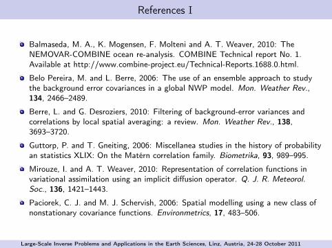
Balmaseda, M. A., K. Mogensen, F. Molteni and A. T. Weaver, 2010: TheNEMOVAR-COMBINE ocean re-analysis. COMBINE Technical report No. 1.Available at http://www.combine-project.eu/Technical-Reports.1688.0.html.

Belo Pereira, M. and L. Berre, 2006: The use of an ensemble approach to studythe background error covariances in a global NWP model. Mon. Weather Rev.,134, 2466–2489.

Berre, L. and G. Desroziers, 2010: Filtering of background-error variances andcorrelations by local spatial averaging: a review. Mon. Weather Rev., 138,3693–3720.

Guttorp, P. and T. Gneiting, 2006: Miscellanea studies in the history of probabilityan statistics XLIX: On the Matérn correlation family. Biometrika, 93, 989–995.

Mirouze, I. and A. T. Weaver, 2010: Representation of correlation functions invariational assimilation using an implicit diffusion operator. Q. J. R. Meteorol.Soc., 136, 1421–1443.

Paciorek, C. J. and M. J. Schervish, 2006: Spatial modelling using a new class ofnonstationary covariance functions. Environmetrics, 17, 483–506.


References II

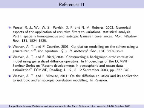
Purser, R. J., Wu, W. S., Parrish, D. F. and N. M. Roberts, 2003. Numericalaspects of the application of recursive filters to variational statistical analysis.Part I: spatially homogeneous and isotropic Gaussian covariances. Mon. WeatherRev., 131, 1524–1535.

Weaver, A. T. and P. Courtier, 2001: Correlation modelling on the sphere using ageneralized diffusion equation. Q. J. R. Meteorol. Soc., 131, 3605–3625.

Weaver, A. T. and S. Ricci, 2004: Constructing a background-error correlationmodel using generalized diffusion operators. In Proceedings of the ECMWFSeminar Series on “Recent developments in atmospheric and ocean dataassimilation”, ECMWF, Reading, U. K., 8–12 September 2003, pp. 327–340.

Weaver, A. T. and I. Mirouze, 2011: On the diffusion equation and its applicationto isotropic and anisotropic correlation modelling. In Revision.


Documents

Background-error correlation modelling in variational ...€¦ · Applications of data assimilation in oceanography Providing initial conditions for climate forecasts. Monthly, seasonal,