Backscattering, extinction, and liquid water contentin fog: a detailed study of their relationsfor use in lidar systems

Glauco Tonna

A solution to the single-scattering lidar equation to infer optical extinction, liquid water content W, andvisibility in a fog through a monostatic pulsed lidar, requires the use of the relations, and combinations ofthem, between backscattering coefficient Al, extinction coefficient a, and W. To this end, 3 and a have beencomputed for 239 droplet size spectra and forty wavelengths from 0.25 to 12 ,ui, together with W, and thethree relations f vs a, W vs a, and a(0.55 ,um) vs a have been determined. The analysis of their behavior withwavelength shows that (1) the relation vs a is mostly reliable in the X = 0. 2 5-2-/im region, where thedispersion of the ,B values around the best-fit curve is within 20%; (2) the relation W vs is generally not wellverified (the dispersion is centered around 30%), and when used in connection with the A vs a relation to inferliquid water content, their joint dispersion PD is always greater than 20%; (3) the relation a(0.55 im) vs a is wellverified in the region X = 0.25-2 ,m (dispersion within 15%), and when used in connection with the a3 vs arelation to infer visibility PD appears to be minimum at _ 0.35 gm (PD = 4.7%).

1. Introduction

For a monostatic pulsed lidar operating at wave-length , the returned power P(R), corresponding to adistance R from the lidar apparatus, is a function ofboth the volume backscattering coefficient A(R) andthe volume extinction coefficient a(R) of the suspend-ed fog droplets. It is customary to define the moreconvenient variable S(R) = ln[R2 X P(R)], in terms ofwhich the single-scattering lidar differential equationis

X d 2 = dS (1)f3 dR dR

Let us assume that we know the signal S(R); Eq. (1)contains two unknown functions and thus its solutionrequires the previous determination of a relation be-tween and a, to eliminate /3 and to solve for a(R).Once a has been determined, if a reliable W vs a rela-tion is available, it is possible to evaluate the liquidwater content W as a function of range R. In a similarway, through a a(0.55 ,um) vs a relation (hereafter,

The author is with CNR Institute of Atmospheric Physics, 31 P. leL. Sturzo, 1-00144 Rome, Italy.

Received 24 July 1989.0003-6935/91/091132-09$05.00/0.© 1991 Optical Socioty of Amorica.

these relations are briefly indicated as -a, W-a, etc.)one can try to evaluate the visibility as a function of R.

Before reviewing previous work concerning theabove quantities and their mutual relations, we notethat the optical properties of clouds or fogs are oftenassumed to be valid for both clouds and fogs, which aretogether referred to as water clouds; this is because fogand cloud spectra are often similar, mainly whenclouds have a limited vertical extent, as do stratusclouds.

Mallow' used forty fog droplet size distributions ofthe gamma type to compute , a, and the ratios /3/a at X= 0.6943,gm. Results showthat 3and avarybyalmost2 orders of magnitude within the distributions used,and the /a ratios have a mean value of 0.0898 sr-' andvary from 0.0796 to 0.0936, with a somewhat more than17% variation.

Derr2 computed the average ratio /a and the rele-vant dispersion coefficient, for a set of sixteen watercloud spectra taken from Deirmendjian,3 at nine laserwavelengths from 0.275 to 10.6,gm. The results showthat the dispersion of the $3/a- ratios is greatest at X 3.75 and 10.6 gim, and least at X = 0.530,0.694, and 1.06

Pinnick et al.4 derived theoretical relations between

a and /3 for water clouds at visible and near infraredwavelengths. The predicted relation at X = 1.06 m isa = 18.2 and agrees within 50% with calculationsbased on 156 measured cloud spectra; at X = 0.6328 gm,

1132 APPLIED OPTICS / Vol. 30, No. 9 / 20 March 1991

a = 17.7 A and agrees within 20% with measurementsmade in water clouds generated in the laboratory.

Dubinski et al. 5 studied the a- relation at X = 0.514Mm, in water clouds of three different types (S,M,L)produced in the laboratory. The relation comes out tobe linear and is given by a = 51 A3, a* = 23 , and a = 20 /for the S, M, and L types of water cloud, respectively.

Jennings 6 measured /3 and of at the CO2 laser wave-length X = 10.591 Am, for water clouds produced in thelaboratory; measurements were found to be within afactor of 2 with the relation a = 3.21 X 103, derivedfrom theory.

Pinnick et al. 7 verified the validity of linear relationsbetween a and W derived from theory, at several wave-lengths in the X = 0.55-12.5-Mm interval, using 341experimental fog spectra; their results show thataround X = 11 Mm the (a,W) data points are strictly inagreement with the predicted relation af = 128W (a inkm-', Win g-m-3 ).

Tonna and Valenti8 studied the -W relation atseventy-four wavelengths from 0.35 to 90 Am, with asample of 239 experimental fog spectra. Results showthat the a-W relation is mostly reliable in the 10-12-Mm X-region, where the correlation coefficient for apower-law fit is between 0.971 and 0.989, and the rela-tive dispersion is within 16%.

Low9 examined the relations a(0.55 Mm)-W, a(0.55Mm)-a-(3 .7 5 Mm), and a(0.55 Mm)-a(10.5 Mm) on thebasis of thirty fog spectra of the gamma and lognormaltype. The regression equation for the first relation isa(0.55 Mm) = 93.2 W06 38 , with correlation coefficient p= 0.997; for the other two relations we have a(3.75 Mm)= 1.487[a-(0.55 Mm)]0.92 8, p 0.999, and a(10.5 Mm) =0.211[a-(0.55 Mm)]1. 378 , p = 0.997.

Once the above-mentioned relations have been de-termined Eq. (1) can be integrated, and some proper-ties of the atmosphere inferred as a function of range.Previous works on this topic are now briefly summa-rized.

Klett' 0 in 1981 presented a new method of integra-tion of Eq. (1), for determining a(R) in an inhomogene-ous atmosphere, which assumes a power-law relationbetween /3 and a of the form a = ciaKl, with cl and K1depending on wavelength, and an upper referencerange Rm, so that the solution is generated for R < Rrn.The suggested solution, given by

a(R) = Rxp( S )

I +( 2 ) JRm (S RSm)

is shown to be stable with respect to perturbations insignal S, in the assumed -a- relation and in the value ofthe extinction estimated at the far-end boundary R.,a. = a(Rr).

Hughes et al.,"1 Measure,12 and Bissonnette1 3 inves-tigated the sensitivity of Eq. (2) to uncertainties in the3-a- relation and in the boundary value a,,,.Ferguson and Stephens,' 4 Mulders,15 and Fernald16

described numerical algorithms for inverting lidar re-

turns, while Klett17 considered a particular boundaryvalue model for estimating arm.

Lindberg et al.18 and Carnuth and Reiter' 9 usedKlett's inversion method to derive optical extinctionprofiles (R) from cloudy and foggy atmospheres at X =0.347, 0.530, 0.694, and 1.06 Am.

In this paper we study the behavior of relations p-a,W-a, and a(0.55 Am)-a in the X = 0.25-12-Mm range,with the aim of locating those wavelengths more suit-able for inferring through lidar techniques, extinction,LWC, and visibility vertical profiles in fog.

II. Computations

Computations were performed on the basis of a sam-ple of 239 experimental size spectra of valley, advec-tion, and radiation fogs taken from the literature,20-27

which had droplet radii ranging from 0.3 to 54 Mm.Forty wavelengths from 0.25 to 12MAm were considered,and those corresponding to the main laser lines wereincluded, namely, 0.4880- and 0.514 -,m (argon laser),0.63 2 8-Mm (He-Ne), 0.69 4 3-Mm (ruby), 1.06-Mm(Nd:YAG), 10.6-Mm (CO2), and the ruby (0.3472 Am)and Nd:YAG (0.5320 Mm) second harmonics.

For each droplet radius distribution f(r) and eachwavelength, the following quantities were computed:

a(X), the volume extinction coefficient, given by

a = m rr2 K[r,m(X)]f(r)dr,frm

(3)

where rn and rM are the lower and upper radii of thef(r) considered, K is the efficiency factor for extinction,and m(X) is the complex refractive index of water.

p(X), the volume backscattering coefficient, given by

: A2 rM ij[7rrm(X)] + i217r,r,m( r)dN3X) = 4?r2 Jrr. 2frd,

where il and i2 are the Mie intensity functions for lightscattered at 0 = 7r.

W, the liquid water content.Data elaboration consisted of:(1) Determining, at each wavelength, the average:

and a, together with the relevant dispersion coefficient(DISP = standard deviation over mean value in per-cent), skewness and kurtosis (a3 and a4 are the thirdand fourth dimensionless moments about the mean,respectively) as well as the average ratio //a and therelevant dispersion coefficient.

(2) Fitting, at eachwavelength, the (/,), (Wa,), and[a-(0.55 Mm),a] data points with power-law functions ofthe form y = cxK and determining the relevant correla-tion coefficients, the dispersion coefficients around thebest-fit curves, the dispersion coefficients pertainingto the regression coefficients c and K, and the degree ofcorrelation between c and K.

(3) Fitting the above data points with a straight lineand determining the relative differences in correlationand dispersion between the nonlinear and the linearcases.

Computations were carried out with an IBM 370 indouble precision (14 digits). Integrations over r in

20 March 1991 / Vol. 30, No. 9 / APPLIED OPTICS 1133

(4)

Eqs. (3) and (4) used steps of Ar = 0.01 Am for X S 6Mmand Ar 0.1 gm for X > 6 Am. Mie efficiency factorsand intensity functions were computed with a programby Wiscombe.28 The complex refractive index ofdroplets was taken from data by Hale and Querry29

concerning pure water, as is generally done in theliterature.4' 6' 7' 1 2' 30 Systematic and complete measure-ments of the chemical composition of fog during itsevolution, together with simultaneous measurementsof droplet spectra, both at ground level and along thevertical, became only recently available,31 and nowallow a realistic estimate of the effect of contaminantson the values of the optical quantities, which by apreliminary evaluation7 should be limited to within afew percent.

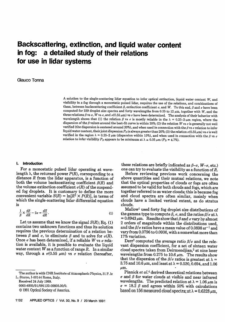
The optical quantities considered present markedvariations with wavelength. This general feature ismainly due to the behavior of the imaginary part of thecomplex refractive index m(X) = n(X) - ik(X) in the X =0.35-7-Am interval. Indeed, while the real part n re-mains almost constant, the imaginary coefficient kvaries over more than 8 orders of magnitude within theconsidered -interval, with well-pronounced maximaand minima at X = 0.5, 1.4, 1.6,2.0,2.2,3.0, 3.8,4.7,5.3,and 6.05Am, which induce corresponding peaks on theoptical quantities.

Not all the computed data are shown in this paper;further details and tables can be found in Ref. 32,which is available from the authors.

Ill. Results

A. Features of the , , //a, and WData

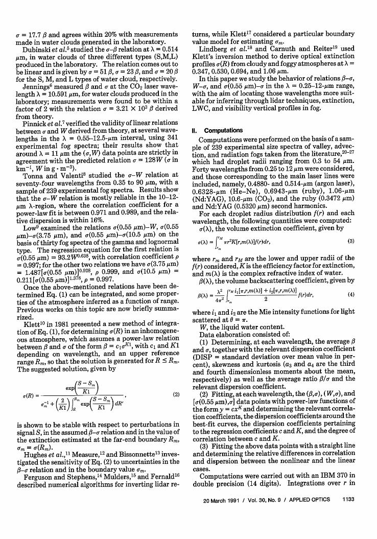
In Figs. 1 and 2 the behavior of the average : and a asa function of , is reported, respectively, together withthe relevant dispersion, skewness, and kurtosis coeffi-cients.

The mean backscattering coefficient fi (Fig. 1) haswell-pronounced minima close to X = 3, 6, and 11 Mm,and it varies over more than 2 orders of magnitudewithin the considered spectral interval. The otherparameters (DISP, a3, a4) also show many oscillations,while their values indicate that the distribution of thefi values around the mean is highly dispersed (DISPcentered around 70%), skewed to the right (a3 > 0), andmore peaked than a normal distribution (a4 > 3).

The mean extinction coefficient Id (Fig. 2) has mini-ma around X = 2.75,6, and 11 m, while it varies withina factor of 1.8 over the whole -range. CoefficientsDISP, a3, and a4 are almost constant with X and cen-tered around 68%, 1, and 3.5, respectively.

Note that the decreasing of fi of 2 orders of magni-tude around X = 3m, as well as the minima around =6 and 11,um, together with the almost constant behav-ior of , might have some implication in the problemsof propagation and possibly of visibility in fog.

The behavior of /a strictly parallels32 that of 3 givenin Fig. 1, while the relevant dispersion coefficientshows maxima at X = 2.85, 3.25, 6, and 10 Am, whereDISP = 38, 48, 70, and 56%, respectively, and minima

8

A

2' * !.

0. __ _ -

u6'68 10 1

u z 4 6 8 lb0 liA (im)

Fig. 1. Behavior, with A, of the average backscattering coefficient and the relevant coefficients of dispersion, skewness, and kurtosis

(DISP, a3, and a4).

80I DISP %1

60.

2 a

. I_____ _____ __________ _____ _____

a:4 :

0 2 4 6A (m)

8 10 12

Fig. 2. Behavior, with X, of the average extinction coefficient -a andthe relevant coefficients of dispersion, skewness, and kurtosis

(DISP, a, and a4).

1134 APPLIED OPTICS / Vol. 30, No. 9 / 20 March 1991

I *o~~~sP (%) --~~N_ __ ____ _

*CORRI

:'1'S - ,11

8c1 (%:IK 8-sca%

6 .

) (M)8 10 - 12

Table I. Correlation Coefficient (CORR1), Dispersion Coefficient(DISP1), and Regression Coefficients (c1 ,K1), as a Function of X for , =

cl.K1 (is in mrn1 sr-, a in mr1)

CORRI DISPI c, - 10' KI

0.2500 0.991 9.45 5.649 1.026

0.3472 0.999 3.49 5.139 0.992

0.4880 0.981 12.94 4.214 0.940

05140 0.977 14.18 4.052 0.929

0.5320 0.975 14.80 4.021 0.926

0.5500 0.972 15.80 3.844 0.918

0.6328 0.965 17.56 3.598 0.900

0.6943 0.961 18.70 3.486 0.897

0.7250 0.957 19.42 3.499 0.893

0.8000 0.956 19.70 3.441 0.890

0.9000 0.958 1937 3.718 0.907

1.0600 0.962 18.25 3.584 0.903

1.4000 0.976 14.78 3.824 0.949

1.6000 0.976 14.58 4.154 0.957

2.0000 0.959 20.48 3.753 1.010

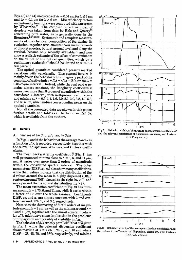
Fig. 3. Behavior, with A, of the correlation and dispersion coeffi-cients (CORRI and DISP1) for = cKl, and of the dispersioncoefficients (6c, and K1) for the regression coefficients cl and K1.

at X = 0.3472,3,3.75,7, and 12 Am, where DISP = 4,25,25, 29, and 27%, respectively.

Finally, the liquid water content computed for the239 spectra of the sample has the following features:W = 0.128 g . m-3, DISP =68%, a3 = 1.3, and a4 = 5.6.

B. Relation 3-a

Figure 3 gives the behavior, with X, of the correlation(CORR1) and dispersion (DISP1) coefficients of thebest-fit curve of the 239 (ha) data points expressed by

0 = CJUKI, (5)

where cl and K1 depend on X; Fig. 3 also gives thespectral behavior of the dispersion coefficients (6c,and 5K1) of the regression coefficients cl and K1.

The types of function usually adopted to express the-a dependence are Eq. (5) and the linear relation ,B =

aja. Some authors 4' 6'7 have found, as summarized inSec. I, that at certain wavelengths the assumption oflinearity was, for practical purposes, consistent withthe data they analyzed. On the other hand, Measure'2

and Klett30 showed, through a simulation of lidar re-turns at X = 1.06 ,um based on measured droplet sizedistributions, that the use of a power law allows greateraccuracy in the determination of a(R) through Eq. (2).Moreover, Klett30 holds that it is more realistic toassume /3 and a as linearly related but with a propor-tionality coefficient a, which depends on a and, on thebasis of droplet size distributions measured in fog andlow clouds, he found a, (a) = 0.0074 + 0.055 exp{-[(lna- 4)/3.1]21. When this expression is used in a simula-tion of lidar returns at X = 1.06 gim, the agreementbetween the recovered and the actual extinction pro-

file is seen to be considerably better than with the useof a power law.

From the values of CORR1 and DISP1 in Fig. 3, itcomes out that Eq. (5) is well verified in the X = 0.25-0.5-,m range, where CORR1 2 0.975 and DISP1 •14%; the best situation occurs at X = 0.35 gim, whereCORR1 = 0.999 and DISP1 = 3.5%. Equation (5) stillappears reliable in the 0.5-2-Am range and around 6.3,gm, where CORR1 > 0.950 and DISP1 • 20%, but isunreliable elsewhere. The dispersion coefficients 6c,and bK1 follow the behavior of DISP1, but their behav-ior is more uniform; the correlation coefficient be-tween cl and K1, r(c,,K1), is practically constant andequal to 0.99, so that its behavior is not reported. Ourfindings concerning Eq. (5) in the X = 0.25-2-gm inter-val, are given in Table I. To verify to what extent thepower-law fit excels the linear one, a straight line hasalso been fitted to the data points; the comparisonbetween the two cases is presented in Sec. III.E.

If we insert Eq. (5) into Eq. (1) and solve with respectto a(R), we obtain Eq. (2). We note that cl does notexplicitly appear in Eq. (2) but it possibly enters theinversion algorithms, while its variations there ap-pear through the corresponding variations of K1, be-cause r(c,,K1) = 0.99.

From the features of the f-a relation with X, itappears that a(X) can be determined, as a function ofrange, with reasonable accuracy in the X = 0.25-2-gminterval. On the other hand, for a definitive evalua-tion of the limits of validity of Eq. (5) in connectionwith its use in Eq. (1), a(R) should be determinedthrough a numerical simulation which, starting from agiven vertical behavior of the droplet size distributionfunction,3 2 computes the behavior of Al, a, and S as afunction of R and X and determines through Eq. (2)a(R) and its dispersion induced by the dispersions 6c,and bK1 of cl and K1.

20 March 1991 / Vol. 30, No. 9 / APPLIED OPTICS 1135

to0

0.8

40

20

C

2C

C

6

a

l.01CORR2

0,

20:1'--

:.'12 **) .

0. _____ _____ _____ _____

0 2 4 6 8 lbA (Um)

Fig. 4. Same as Fig. 3 except for W = c2 UK2.

1.0

0.8

40

20

0.

1.0'

nlR.

]

40

20'

0.

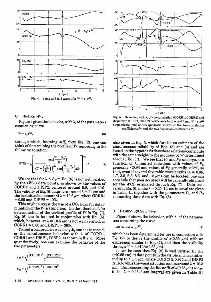
C. Relation W-

Figure 4 gives the behavior, with X, of the parametersconcerning curve

W = c2o 2,

PC

PCI4

1 ~~~~~~~~~~0 A P 6

A (pm )8 ' 10 12

Fig. 5. Behavior, with , of the correlation (CORR1, CORR2) anddispersion (DISPI, DISP2) coefficients for A = caKl and W = c 2aK2respectively, and of the quadratic means of the two correlation

coefficients Pc and the two dispersion coefficients PD.

(6)

through which, knowing o-(R) from Eq. (2), one canthink of determining the profile of W, according to thefollowing equation:

exp S1Sm)]2

W(R) = C2-L 1 + ( ) R exp(S m)dRf

We see that for X < 8 m Eq. (6) is not well verifiedby the (Wo) data points, as shown by the values ofCORR2 and DISP2, centered around 0.9, and 30%.The validity of Eq. (6) improves around X = 11 um andthe best situation occurs at X = 10.6 Am, where CORR2= 0.99 and DISP2 = 10%.

This might suggest the use of a C02 lidar for deter-mination of the W(R) function. On the other hand, fordetermination of the vertical profile of W in Eq. (7),Eq. (6) has to be used in conjunction with Eq. (5),which, however, at X = 10.6 m is not well verified, asCORR1 = 0.86 and DISP = 36%.

To find a compromise wavelength, one has to consid-er the simultaneous behavior with X of CORR1,CORR2 and DISPI, DISP2, as shown in Fig. 5. Morequantitatively, one can examine the behavior of thetwo parameters

C (CORR1) 2 + (CORR2) 2

2

PD = (DISP1)2 + (DISP2)2

2

also given in Fig. 5, which furnish an estimate of thesimultaneous reliability of Eqs. (5) and (6) and arebased on the hypothesis that these relations contributewith the same weight to the accuracy of W determinedthrough Eq. (7). We see that PC and PD undergo, as afunction of , limited variations with values of PCgenerally <0.93 and values of PD generally >25%, sothat, even if several favorable wavelengths (A = 0.35,1.7, 3.5, 6.3, 8.5, and 12 m) can be located, one canconclude that poor accuracy will be generally obtainedfor the W(R) estimated through Eq. (7). Data con-cerning Eq. (6) in the X = 0 .25-12-,m interval are givenin Table II, together with the parameters P and PDconnecting these data with Eq. (5).

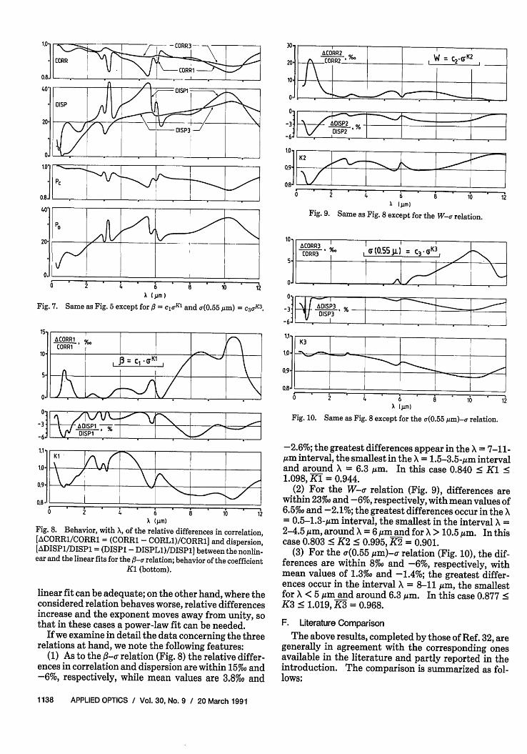
D. Relation uoj.55 m)-cr

Figure 6 shows the behavior, with A, of the parame-ters concerning the curve

a(0.55 Am) = C3aK3, (8)

which has been determined for use in connection withEq. (2) to derive the profile of (0.55 m) with anexpression similar to Eq. (7), and then the visibilitythrough V = 3.912/u(0.55 Mm).

It can be seen that Eq. (8) is well verified by the(W0.55 m),a) data points in the visible and near infra-red up to X - 2 m, where CORR3 0.975 and DISP3< 15%, while the worst situation occurs around X = 10.5,m. Data concerning the linear fit of (0.55,Mm) = a-in the = 0.25-3-Mum interval are given in Table III

1136 APPLIED OPTICS / Vol. 30, No. 9 / 20 March 1991

_ _

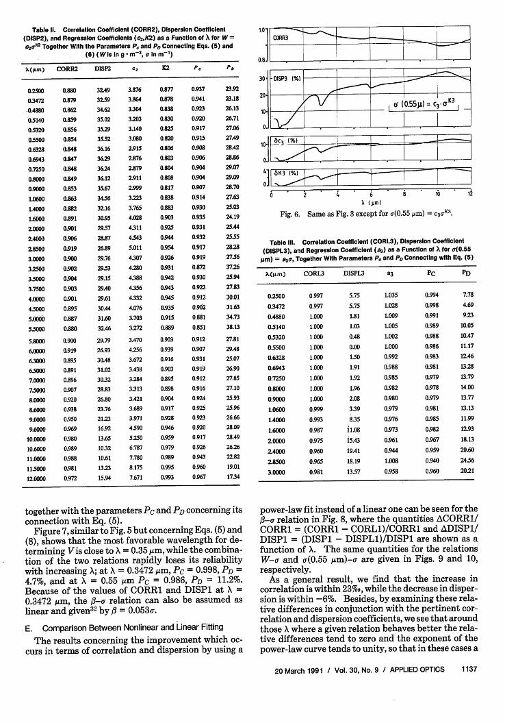
Table II. Correlation Coefficient (CORR2), Dispersion Coefficient(DISP2), and Regression Coefficients (c2,K2) as a Function of X for W =c2a02 Together With the Parameters P. and PD Connecting Eqs. (5) and

(6) (W Is in g m 3 , o n m 1)

X(m) CORR2 DISP2 C2 K2 PC PD

0.2500

0.3472

.0.4880

0514005320055000.6328

0.6943

0.7250

0.8000

0.9000

1.0600

1.4000

1.6000

2.0000

2.4000

2.8500

3.0000

3.2500

350003.7500

4.0000

450005.0000

55000

5.8000

6.0000

63000650007.0000

750008.0000

8.6000

9.0000

9.6000

10.0000

10.6000

11.0000

115000

12.0000

0.880

0.879

0.862

0.859

0.856

0.854

0.848

0.847

0.848

0.849

0.853

0.863

0.882

0.891

0.901

0.906

0.919

0.900

0.902

0.904

0.903

0.901

0.895

0.887

0.880

0.900

0.919

0.895

0.891

0.896

0.907

0.920

0.938

0.950

0.969

0.980

0.989

0.988

0.981

0.972

32.49

325934.62

35.02

35.29

35.52

36.16

36.29

36.24

36.12

35.67

34.56

32.16

30.95

29.57

28.87

26.89

29.76

295329.15

29A0

29.61

30.44

31.60

32.46

29.79

26.93

30A831.02

30.32

28.83

26.80

23.76

21.23

16.92

13.65

10.32

10.61

13.23

15.94

3.876

3.864

3.304

3.203

3.140

3.080

2.915

2.876

2.879

2.911

2.999

3.223

3.765

4.028

4.311

4.543

5.011

4.307

4.280

4.388

4.356

4.332

4.076

3.703

3.272

3.470

4.256

3.672

3.438

3.284

3.313

3.421

3.689

3.971

4.590

5.250

6.787

7.780

8.175

7.671

0.877

0.878

0.838

0.830

0.825

0.820

0.806

0.803

0.804

0.808

0.817

0.838

0.883

0.903

0.925

0.944

0.954

0.926

0.931

0.942

0.943

0.945

0.935

0.915

0.889

0.903

0.939

0.916

0.903

0.895

0.898

0.904

0.917

0.928

0.946

0.959

0.979

0.989

0.995

0.993

0.937

0.941

0.923

0.920

0.917

0.915

0.908

0.906

0.904

0.904

0.907

0.914

0.930

0.935

0.931

0.932

0.917

0.919

0.872

0.930

0.922

0.912

0.902

0.881

0.851

0.912

0.907

0.931

0.919

0.912

0.916

0.924

0.925

0.923

0.920

0.917

0.926

0.943

0.960

0.967

23.92

23.18

26.13

26.71

27.06

27.49

28.42

28.86

29.07

29.09

28.70

27.63

25.03

24.19

25.44

2555

28.28

275637.26

25.94

27.83

30.01

31.63

34.73

38.13

27.81

29.48

25.07

26.90

27.85

27.10

25.93

25.96

26.66

28.09

28A9

26.26

22.82

19.01

17.34

1.0I

una

CORR3 -f

30 OISP3(%C

roll ar I (0155j1) C3 GI 20.

010

10 6C3 (%N__

0.

0 ,-

6 2 4. .. . . . . . . .6

6(m)

Fig. 6. Same as Fig. 3 except for a(0.55 gm) = c3 aKS.

Table il. Correlation Coefficlent (CORL3), Dispersion Coefficient(DISPL3), and Regression Coefficlent (a3) as a Function of X for a(0.55

pm) = a3a, Together With Parameters PC and PD Connecting with Eq. (5)

XG(-m) CORL3 DISPL3 a3 PC PD

0.2500 0.997 5.75 1.035 0.994 7.78

0.3472 0.997 5.75 1.028 0.998 4.69

0.4880 1.000 1.81 1.009 0.991 9.23

05140 1.000 1.03 1.005 0.989 10.05

05320 1.000 0.48 1.002 0.988 10A7

05500 1.000 0.00 1.000 0.986 11.17

0.6328 1.000 1.50 0.992 0.983 12A6

0.6943 1.000 1.91 0.988 0.981 13.28

0.7250 1.000 1.92 0.985 0.979 13.79

0.8000 1.000 1.96 0.982 0.978 14.00

0.9000 1.000 2.08 0.980 0.979 13.77

1.0600 0.999 3.39 0.979 0.981 13.13

lA000 0.993 8.35 0.976 0.985 11.99

1.6000 0.987 il.08 0.973 0.982 12.93

2.0000 0.975 15.43 0.961 0.967 18.13

2.4000 0.960 19.41 0.944 0.959 20.60

2.8500 0.965 18.19 1.008 0.940 2456

3.0000 0.981 13.57 0.958 0.960 20.21

together with the parameters PC and PD concerning itsconnection with Eq. (5).

Figure 7, similar to Fig. 5 but concerning Eqs. (5) and(8), shows that the most favorable wavelength for de-termining V is close to X = 0.35 Am, while the combina-tion of the two relations rapidly loses its reliabilitywith increasing X; at X = 0.3472 Am, PC = 0.998, PD =4.7%, and at X = 0.55 ,um PC = 0.986, PD = 11.2%.Because of the values of CORR1 and DISP1 at X =0.3472 Asm, the fl- relation can also be assumed aslinear and given32 by fi = 0.053a.

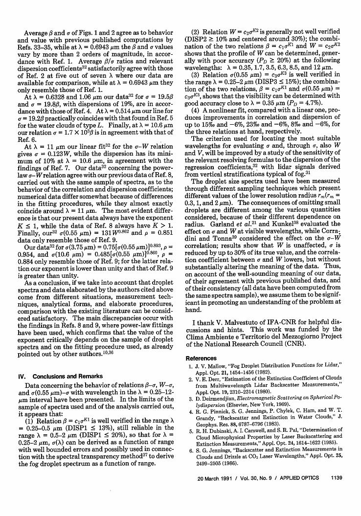
E. Comparison Between Nonlinear and Linear Fitting

The results concerning the improvement which oc-curs in terms of correlation and dispersion by using a

power-law fit instead of a linear one can be seen for thef-c relation in Fig. 8, where the quantities ACORR1/CORR1 = (CORR1 - CORL1)/CORR1 and ADISPl/DISP1 = (DISP1 - DISPL1)/DISP1 are shown as afunction of X. The same quantities for the relationsW-a and a(0.55 Am)-a are given in Figs. 9 and 10,respectively.

As a general result, we find that the increase incorrelation is within 23%o, while the decrease in disper-sion is within -6%. Besides, by examining these rela-tive differences in conjunction with the pertinent cor-relation and dispersion coefficients, we see that aroundthose X where a given relation behaves better the rela-tive differences tend to zero and the exponent of thepower-law curve tends to unity, so that in these cases a

20 March 1991 / Vol. 30, No. 9 / APPLIED OPTICS 1137

1.0*

PC

) . . I _ _ _ _ _ _ _ _ _ _

40'

2 0 - _ _ _ _ _ _ _ _ _ _ _ __ _ _ _ _ _

A. * * & &

A (Jim)Fig. 7. Same as Fig. 5 except for # = ClGK1 and (0.55 Am) = c3aK3.

1.1-

1.0-

0.9.

0.8*

Kl ,,

0 2 6 10 12x (pm)

Fig. 8. Behavior, with A, of the relative differences in correlation,[ACORR1/CORR1 = (CORR1 - CORL1)/CORR11 and dispersion,[ADISPl/DISP1 = (DISP1 - DISPL1)/DISPI] between the nonlin-ear and the linear fits for the ,-o relation; behavior of the coefficient

Ki (bottom).

linear fit can be adequate; on the other hand, where theconsidered relation behaves worse, relative differencesincrease and the exponent moves away from unity, sothat in these cases a power-law fit can be needed.

If we examine in detail the data concerning the threerelations at hand, we note the following features:

(1) As to the -a relation (Fig. 8) the relative differ-ences in correlation and dispersion are within 15%o and-6%, respectively, while mean values are 3.8oo and

30.

20-

10.

0

I _ 1 1 ,

(m)

Fig. 9. Same as Fig. 8 except for the W-a relation.

10. A R I I F

EORR3 Is O55 IL) C3 (5K)1

(3 9

1.0 .

0.9.

0.8'6 2 4

(LM)

6 .- . -8 l 12

Fig. 10. Same as Fig. 8 except for the a(0.55 lum)-a relation.

-2.6%; the greatest differences appear in the X = 7-11-,m interval, the smallest in the X = 1.5- 3.5-Am intervaland around X = 6.3 m. In this case 0.840 K1 1.098, K1 = 0.944.

(2) For the W-c relation (Fig. 9), differences arewithin 23%o and -6%, respectively, with mean values of6.5%o and -2.1%; the greatest differences occur in the X= 0 .5-1.3-Am interval, the smallest in the interval X =2-4.5 m, around X = 6um and for X > 10.5 m. In thiscase 0.803 K2 0.995, K2 = 0.901.

(3) For the (0.55,Mm)-c relation (Fig. 10), the dif-ferences are within 8%o and -6%, respectively, withmean values of 1.3%o and -1.4%; the greatest differ-ences occur in the interval X = 8-11 Am, the smallestfor X < 5 m and around 6.3 m. In this case 0.877 K3 1.019, K3 = 0.968.

F. Literature Comparison

The above results, completed by those of Ref. 32, aregenerally in agreement with the corresponding onesavailable in the literature and partly reported in theintroduction. The comparison is summarized as fol-lows:

1138 APPLIED OPTICS / Vol. 30, No. 9 / 20 March 1991

OI SI ________

l l l - l

, _ .

.

I ! s I HE

Pi

I

I

0 2 4 6

V'110. . V\.-

-3 1 __2RL' %-6 DISPI

Average fi and a of Figs. 1 and 2 agree as to behaviorand value with previous published computations byRefs. 33-35, while at X = 0.6943,um the f and a valuesvary by more than 2 orders of magnitude, in accor-dance with Ref. 1. Average l/ ratios and relevantdispersion coefficients32 satisfactorily agree with thoseof Ref. 2 at five out of seven X where our data areavailable for comparison, while at X = 0.6943 Am theyonly resemble those of Ref. 1.

At X = 0.6328 and 1.06 Am our data3 2 for a = 19.5,Band a = 19.83, with dispersions of 19%, are in accor-dance with those of Ref.4. At X = 0.514,um our line fora = 19.2f practically coincides with that found in Ref. 5for the water clouds of type L. Finally, at X = 10.6 mour relation ar = 1.7 X 103 is in agreement with that ofRef. 6.

At X = 11 m our linear fit32 for the o-W relationgives a = 0.123W, while the dispersion has its mini-mum of 10% at X = 10.6 m, in agreement with thefindings of Ref. 7. Our data3 2 concerning the power-law cr-W relation agree with our previous data of Ref. 8,carried out with the same sample of spectra, as to thebehavior of the correlation and dispersion coefficients;numerical data differ somewhat because of differencesin the fitting procedures, while they almost exactlycoincide around X = 11 m. The most evident differ-ence is that our present data always have the exponentK S 1, while the data of Ref. 8 always have K > 1.Finally, our3 2 a(0.55 Am) = 131W0 86 2 and p = 0.851data only resemble those of Ref. 9.

Our data32 for a(3.75 Am) = 0.75[a.(0.55 Mm)]0 893 , p =0.954, and a(10.6 Am) = 0.485[ao(0.55 Mm)]0 860, p =

0.884 only resemble those of Ref. 9; for the latter rela-tion our exponent is lower than unity and that of Ref. 9is greater than unity.

As a conclusion, if we take into account that dropletspectra and data elaborated by the authors cited abovecome from different situations, measurement tech-niques, analytical forms, and elaborate procedures,comparison with the existing literature can be consid-ered satisfactory. The main discrepancies occur withthe findings in Refs. 8 and 9, where power-law fittingshave been used, which confirms that the value of theexponent critically depends on the sample of dropletspectra and on the fitting procedure used, as alreadypointed out by other authors.1036

IV. Conclusions and Remarks

Data concerning the behavior of relations p-a, W-a,and a(0.55 ,m)-a with wavelength in the X = 0.25-12-Mm interval have been presented. In the limits of thesample of spectra used and of the analysis carried out,it appears that:

(1) Relation ,B = ciaK' is well verified in the range X= 0.25-0.5 Am (DISP1 < 13%), still reliable in therange X = 0.5-2 Am (DISPI < 20%), so that for X =0.25-2 ,m, a(X) can be derived as a function of rangewith well bounded errors and possibly used in connec-tion with the spectral transparency method37 to derivethe fog droplet spectrum as a function of range.

(2) Relation W = c2crK2 is generally not well verified(DISP2 ' 10% and centered around 30%); the combi-nation of the two relations = cKl and W = c2 UK2

shows that the profile of W can be determined, gener-ally with poor accuracy (PD 2 20%) at the followingwavelengths: X = 0.35, 1.7, 3.5, 6.3, 8.5, and 12/im.

(3) Relation (0.55 Am) = c3 aK3 is well verified inthe range X = 0.25-2 Am (DISP3 • 15%); the combina-tion of the two relations, 3 = cKl and o(0.55 Mm) =c3 aK3, shows that the visibility can be determined withgood accuracy close to X = 0.35 gm (PD = 4.7%).

(4) A nonlinear fit, compared with a linear one, pro-duces improvements in correlation and dispersion ofup to 15%o and -6%, 23%o and -6%, 8%o and -6%, forthe three relations at hand, respectively.

The criterion used for locating the most suitablewavelengths for evaluating a and, through a, also Wand V, will be improved by a study of the sensitivity ofthe relevant resolving formulas to the dispersion of theregression coefficients,32 with lidar signals derivedfrom vertical stratifications typical of fog.31

The droplet size spectra used have been measuredthrough different sampling techniques which presentdifferent values of the lower resolution radius rm(rm =0.3, 1, and 2 Mm). The consequences of omitting smalldroplets are different among the various quantitiesconsidered, because of their different dependence onradius. Garland et al. 21 and Kunkel38 evaluated theeffect on a and W at visible wavelengths, while Corra-dini and Tonna39 considered the effect on the a-Wcorrelation; results show that W is unaffected, a isreduced by up to 30% of its true value, and the correla-tion coefficient between a and W lowers, but withoutsubstantially altering the meaning of the data. Thus,on account of the well-sounding meaning of our data,of their agreement with previous published data, andof their consistency (all data have been computed fromthe same spectra sample), we assume them to be signif-icant in promoting an understanding of the problem athand.

I thank V. Malvestuto of IFA-CNR for helpful dis-cussions and hints. This work was funded by theClima Ambiente e Territorio del Mezzogiorno Projectof the National Research Council (CNR).

References1. J. V. Mallow, "Fog Droplet Distribution Functions for Lidar,"

Appl. Opt. 21, 1454-1456 (1982).2. V. E. Derr, "Estimation of the Extinction Coefficient of Clouds

from Multiwavelength Lidar Backscatter Measurements,"Appl. Opt. 19, 2310-2314 (1980).

3. D. Deirmendjian, Electromagnetic Scattering on Spherical Po-lydispersion (Elsevier, New York, 1969).

4. R. G. Pinnick, S. G. Jennings, P. Chylek, C. Ham, and W. T.Grandy, "Backscatter and Extinction in Water Clouds," J.Geophys. Res. 88, 6787-6796 (1983).

5. R. H. Dubinski, A. I. Carswell, and S. R. Pal, "Determination ofCloud Microphysical Properties by Laser Backscattering andExtinction Measurements," Appl. Opt. 24, 1614-1622 (1985).

6. S. G. Jennings, "Backscatter and Extinction Measurements inClouds and Drizzle at CO2 Laser Wavelengths," Appl. Opt. 25,

2499-2505 (1986).

20 March 1991 / Vol. 30, No. 9 / APPLIED OPTICS 1139

7. R. G. Pinnick, S. G. Jennings, P. Chylek, and H. J. Auvermann,"Verification of a Linear Relation Between IR Extinction, Ab-sorption and Liquid Water Content of Fogs," J. Atmos. Sci. 36,1577-1586 (1979).

8. G. Tonna and C. Valenti, "Optical Attenuation Coefficients andLiquid Water Content Relationship in Fog, at Seventy-FourWavelengths from 0.35 to 90 um," Atmos. Environ. 17, 2075-2080 (1983).

9. R. D. H. Low, "A Theoretical Investigation of Cloud/Fog Extinc-tion Coefficients and Their Spectral Correlations," Contrib.Atmos. Phys. 52, 44-57 (1979).

10. J. D. Klett, "Stable Analytical Inversion Solution for ProcessingLidar Returns," Appl. Opt. 20, 211-220 (1981).

11. H. G. Hughes, J. A. Ferguson, and D. H. Stephens, "Sensitivityof a Lidar Inversion Algorithm to Parameters Relating Atmo-spheric Backscatter and Extinction," Appl. Opt. 24, 1609-1613(1985).

12. E. M. Measure, "Effect of Backscatter-to-Extinction Ratio onLidar Inversions," in Abstracts, Thirteenth International Con-ference on Laser Radar (NASA Conference Publication 2431,Toronto, Ontario, Canada, 1986).

13. L. R. Bissonnette, "Sensitivity.Analysis of Lidar Inversion Al-gorithms," Appl. Opt. 25, 2122-2125 (1986).

14. J. A. Ferguson and D. H. Stephens, "Algorithm for InvertingLidar Returns," Appl. Opt. 22, 3673-3675 (1983).

15. J. M. Mulders, "Algorithm for Inverting Lidar Returns: Com-ments," Appl. Opt. 23, 2855-2856 (1984).

16. F. G. Fernald, "Analysis of Atmospheric Lidar Observations:Some Comments," Appl. Opt. 23, 652-653 (1984).

17. J. D. Klett, "Lidar Calibration and Extinction Coefficients,"Appl. Opt. 22, 514-515 (1983).

¶8. J. D. Lindberg, W. J. Lentz, E. M. Measure, and R. Rubio, "LidarDeterminations of Extinction in Stratus Clouds," Appl. Opt. 23,2172-2177 (1984).

19. W. Carnuth and R. Reiter, "Cloud Extinction Profile Measure-ments by Lidar Using Klett's Inversion Method," Appl. Opt. 25,2899-2907 (1986).

20. J. A. Garland, "Some Fog Droplet Size Distributions Obtainedby an Impaction Method," Q. J. R. Meteorol. Soc. 97, 483-494(1971).

21. J. A. Garland, J. R. Branson, and L. C. Cox, "A Study of theContribution of Pollution to Visibility in a Radiation Fog,"Atmos. Environ. 7, 1079-1092 (1973).

22. W. C. Kocmond, "Dissipation of Natural Fog in the Atmosphere,Progress of NASA Research on Warm Fog Properties and Modi-fication Concepts," NASA Spec. Publ. SP-212 (1969), p. 57.

23. M. Kumai, "Artic Fog Droplet Size Distribution and Its Effectson Light Attenuation," J. Atmos. Sci. 30, 635-643 (1973).

24. B. A. Kunkel, "Fog Drop-Size Distributions Measured with aLaser Hologram Camera," J. Appl. Meteorol. 10, 482-486(1971).

25. E. J. Mack and R. J. Pilie, "The Microstructure of Radiation Fogat Travis Air Force Base," AFCRL-TR-730609, Calspan ReportCJ-5076-M-2, Calspan Corp., Buffalo, NY (1973).

26. R. J. Pilie, W. J. Eadie, E. J. Mack, C. W. Rogers, and W. C.Kocmond, "Project Fog Drops, Part I: Investigation of WarmFog Properties," NASA Contract Rep. CR-2078 (1972).

27. C. W. Rogers, E. J. Mack, and U. Katz, "The Life Cycle ofCalifornia Coastal Fog Onshore," AFCRL-TR-74-0419, CalspanReport CJ-5076-M-3, Calspan Corp., Buffalo, NY (1974).

28. W. J. Wiscombe, "Mie Scattering Calculations: Advances inTechnique and Fast, Vector-Speed Computer Code," TN-140+STR, NCAR, Boulder, CO (1979).

29. G. M. Hale and M. R. Querry, "Optical Constants of Water in the200-nm to 200-jum Wavelength Region," Appl. Opt. 12,555-563(1973).

30. J. D. Klett, "Lidar Inversion with Variable Backscatter/Extinc-tion Ratios," Appl. Opt. 24, 1638-1643 (1985).

31. S. Fuzzi, G. Orsi, G. Nardini, M. C. Facchini, M. Mariotti, S.McLaren, and E. McLaren, "Heterogeneous Processes in PoValley Radiation Fog," J. Geophys. Res. 93, 11,141-11,151(1988).

32. G. Tonna and V. Malvestuto, "Numerical Data Concerning theRelations Between Backscattering, Extinction and LWC inFog," IFA, Scientific Report (1991).

33. W. Zdunkowski and R. F. Strand, "Light Scattering Constantsfor a Water Cloud," Pageoph 74, 110-133 (1969).

34. D. Deirmendjian, "Far-infrared and Submillimeter Wave At-tenuation by Clouds and Rain," J. Appl. Meteorol. 14, 1584-1593 (1975).

35. E. P. Shettle and R. W. Fenn, "Models for the Aerosols of theLower Atmosphere and the Effects of the Humidity Variationson Their Optical Properties," AFGL-TR-70-0214 (Air ForceGeophysics Laboratory, Hanscom AFB, MA, 1979).

36. R. G. Pinnick, D. L. Hoihjelle, G. Fernandez, E. B. Stenmark, J.D. Lindberg, and G. B. Hoidale, "Vertical Structure in Atmo--spheric Fog and Haze and Its Effects on Visible and InfraredExtinction," J. Atmos. Sci. 35, 2020-2032 (1978).

37. K. S. Shifrin, Physical Optics of Ocean Water (AIP, New York,1988).

38. B. A. Kunkel, "Comparison of Fog Drop Size Spectra Measuredby Light Scattering and Impaction Techniques," AFGL-TR-81-0049 (Air Force Geophysics Laboratory, Hanscom AFB, MA,1981).

39. C. Corradini and G. Tonna, "Absorption and Liquid WaterContent Relationship in Fog, at Thirteen IR Wavelengths,"Atmos. Environ. 15, 271-275 (1981).

1140 APPLIED OPTICS / Vol. 30, No. 9 / 20 March 1991