Once, or twice, though you should fail,Try, try again;

If you would, at last, prevail,Try, try again;

If we strive, ’tis no disgrace.Though we may not win the race;What should you do in that case?

Try, try again.— Thomas H. Palmer, The Teacher’s Manual: Being an Exposition

of an Efficient and Economical System of EducationSuited to the Wants of a Free People (1840)

I dropped my dinner, and ran back to the laboratory. There, in my excitement, I tastedthe contents of every beaker and evaporating dish on the table. Luckily for me, nonecontained any corrosive or poisonous liquid.

— Constantine Fahlberg on his discovery of saccharin,Scientific American (1886)

CHAPTER 2Backtracking

ÆÆÆStill in progress.This chapter describes another recursive algorithm strategy called backtracking. A back-tracking algorithm tries to build a solution to a computational problem incrementally,one small piece at a time. Whenever the algorithm needs to decide between multiplealternatives to the next component of the solution, it simply tries all possible optionsrecursively.

2.1 n Queens

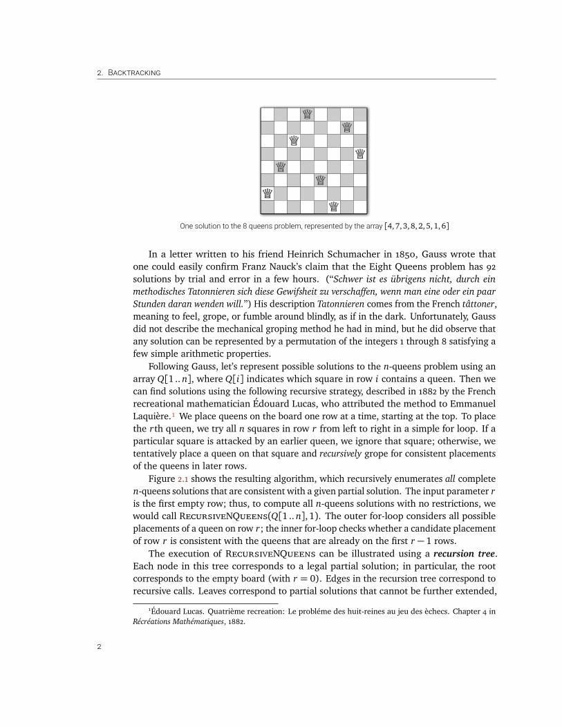
The prototypical backtracking problem is the classical n Queens Problem, first proposedby German chess enthusiast Max Bezzel in 1848 (under his pseudonym “Schachfreund”)for the standard 8× 8 board and by François-Joseph Eustache Lionnet in 1869 for themore general n× n board. The problem is to place n queens on an n× n chessboard,so that no two queens can attack each other. For readers not familiar with the rules ofchess, this means that no two queens are in the same row, column, or diagonal.

© Copyright 2016 Jeff Erickson.This work is licensed under a Creative Commons License (http://creativecommons.org/licenses/by-nc-sa/4.0/).Free distribution is strongly encouraged; commercial distribution is expressly forbidden.See http://jeffe.cs.illinois.edu/teaching/algorithms/ for the most recent revision. 1

2. BACKTRACKING

One solution to the 8 queens problem, represented by the array [4, 7,3, 8,2, 5,1,6]

In a letter written to his friend Heinrich Schumacher in 1850, Gauss wrote thatone could easily confirm Franz Nauck’s claim that the Eight Queens problem has 92solutions by trial and error in a few hours. (“Schwer ist es übrigens nicht, durch einmethodisches Tatonnieren sich diese Gewifsheit zu verschaffen, wenn man eine oder ein paarStunden daran wenden will.”) His description Tatonnieren comes from the French tâttoner,meaning to feel, grope, or fumble around blindly, as if in the dark. Unfortunately, Gaussdid not describe the mechanical groping method he had in mind, but he did observe thatany solution can be represented by a permutation of the integers 1 through 8 satisfying afew simple arithmetic properties.

Following Gauss, let’s represent possible solutions to the n-queens problem using anarray Q[1 .. n], where Q[i] indicates which square in row i contains a queen. Then wecan find solutions using the following recursive strategy, described in 1882 by the Frenchrecreational mathematician Édouard Lucas, who attributed the method to EmmanuelLaquière.¹ We place queens on the board one row at a time, starting at the top. To placethe rth queen, we try all n squares in row r from left to right in a simple for loop. If aparticular square is attacked by an earlier queen, we ignore that square; otherwise, wetentatively place a queen on that square and recursively grope for consistent placementsof the queens in later rows.

Figure 2.1 shows the resulting algorithm, which recursively enumerates all completen-queens solutions that are consistent with a given partial solution. The input parameter ris the first empty row; thus, to compute all n-queens solutions with no restrictions, wewould call RecursiveNQueens(Q[1 .. n], 1). The outer for-loop considers all possibleplacements of a queen on row r; the inner for-loop checks whether a candidate placementof row r is consistent with the queens that are already on the first r − 1 rows.

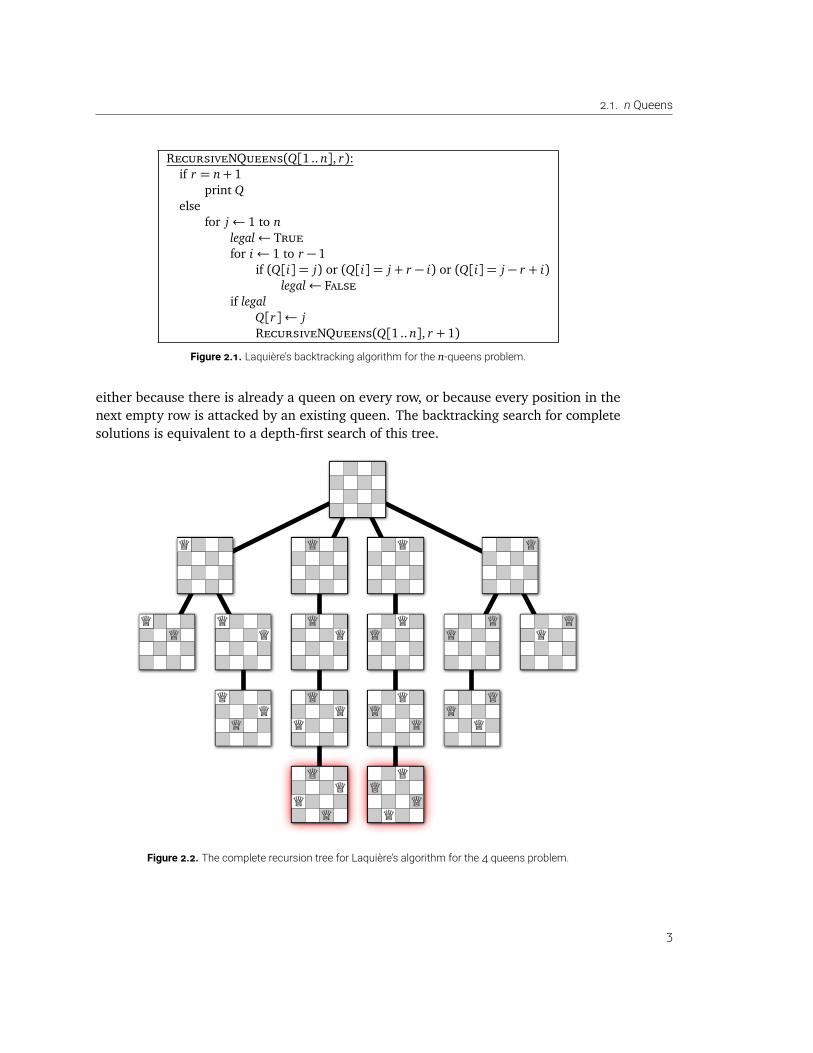
The execution of RecursiveNQueens can be illustrated using a recursion tree.Each node in this tree corresponds to a legal partial solution; in particular, the rootcorresponds to the empty board (with r = 0). Edges in the recursion tree correspond torecursive calls. Leaves correspond to partial solutions that cannot be further extended,

1Édouard Lucas. Quatrième recreation: Le probléme des huit-reines au jeu des èchecs. Chapter 4 inRécréations Mathématiques, 1882.

2

2.1. n Queens

RecursiveNQueens(Q[1 .. n], r):if r = n+ 1

print Qelse

for j← 1 to nlegal← Truefor i← 1 to r − 1

if (Q[i] = j) or (Q[i] = j + r − i) or (Q[i] = j − r + i)legal← False

if legalQ[r]← jRecursiveNQueens(Q[1 .. n], r + 1)

Figure 2.1. Laquière’s backtracking algorithm for the n-queens problem.

either because there is already a queen on every row, or because every position in thenext empty row is attacked by an existing queen. The backtracking search for completesolutions is equivalent to a depth-first search of this tree.

Figure 2.2. The complete recursion tree for Laquière’s algorithm for the 4 queens problem.

3

2. BACKTRACKING

2.2 Game Trees

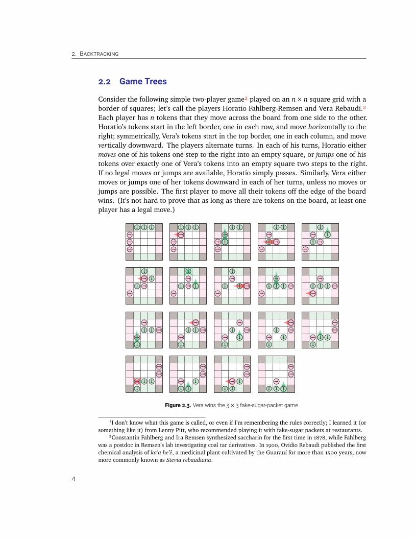
Consider the following simple two-player game² played on an n× n square grid with aborder of squares; let’s call the players Horatio Fahlberg-Remsen and Vera Rebaudi.³Each player has n tokens that they move across the board from one side to the other.Horatio’s tokens start in the left border, one in each row, and move horizontally to theright; symmetrically, Vera’s tokens start in the top border, one in each column, and movevertically downward. The players alternate turns. In each of his turns, Horatio eithermoves one of his tokens one step to the right into an empty square, or jumps one of histokens over exactly one of Vera’s tokens into an empty square two steps to the right.If no legal moves or jumps are available, Horatio simply passes. Similarly, Vera eithermoves or jumps one of her tokens downward in each of her turns, unless no moves orjumps are possible. The first player to move all their tokens off the edge of the boardwins. (It’s not hard to prove that as long as there are tokens on the board, at least oneplayer has a legal move.)

↓

↓ ↓ ↓→→→

↓ ↓ ↓

→→

↓ ↓→

→→

↓

↓ ↓→

→↓

↓→

→→

↓

↓↓

→→

↓

↓→→

→↓

↓→

→→

↓ ↓→

→→

↓ ↓ ↓→

→

↓ ↓→

→→

↓

↓ ↓ →→

↓

↓→

→→

↓

↓↓

→→

↓↓

→→

→

↓↓ ↓

→→

→↓

↓

→→

→↓ ↓

↓

→→

↓ ↓

→→

→

→

→→

→

→ →

→

↓↓

↓ ↓

↓↓ ↓

↓ ↓

Figure 2.3. Vera wins the 3× 3 fake-sugar-packet game.2I don’t know what this game is called, or even if I’m remembering the rules correctly; I learned it (or

something like it) from Lenny Pitt, who recommended playing it with fake-sugar packets at restaurants.3Constantin Fahlberg and Ira Remsen synthesized saccharin for the first time in 1878, while Fahlberg

was a postdoc in Remsen’s lab investigating coal tar derivatives. In 1900, Ovidio Rebaudi published the firstchemical analysis of ka’a he’ê, a medicinal plant cultivated by the Guaraní for more than 1500 years, nowmore commonly known as Stevia rebaudiana.

4

2.2. Game Trees

Unless you’ve seen this game before⁴, you probably don’t have any idea how to play itwell. Nevertheless, there is a relatively simple backtracking algorithm that can play thisgame—or any two-player game without randomness or hidden information—perfectly.That is, if we drop you into the middle of a game, and it is possible to win against anotherperfect player, the algorithm will tell you how to win.

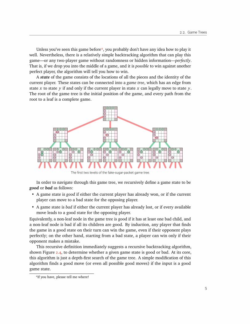
A state of the game consists of the locations of all the pieces and the identity of thecurrent player. These states can be connected into a game tree, which has an edge fromstate x to state y if and only if the current player in state x can legally move to state y .The root of the game tree is the initial position of the game, and every path from theroot to a leaf is a complete game.

↓ ↓ ↓→→→

↓ ↓ ↓

→→

→↓ ↓ ↓

→

→→

↓ ↓ ↓

→→

→

↓ ↓→

→→

↓

↓ ↓→

→→

↓↓ ↓→

→→

↓↓ ↓

→→

→

↓↓ ↓

→→

→

↓↓ ↓

→→

→

↓↓ ↓

→→

→

↓↓ ↓

→→

→

↓↓ ↓

→→

→

↓

The first two levels of the fake-sugar-packet game tree.In order to navigate through this game tree, we recursively define a game state to be

good or bad as follows:• A game state is good if either the current player has already won, or if the current

player can move to a bad state for the opposing player.

• A game state is bad if either the current player has already lost, or if every availablemove leads to a good state for the opposing player.

Equivalently, a non-leaf node in the game tree is good if it has at least one bad child, anda non-leaf node is bad if all its children are good. By induction, any player that findsthe game in a good state on their turn can win the game, even if their opponent playsperfectly; on the other hand, starting from a bad state, a player can win only if theiropponent makes a mistake.

This recursive definition immediately suggests a recursive backtracking algorithm,shown Figure 2.4, to determine whether a given game state is good or bad. At its core,this algorithm is just a depth-first search of the game tree. A simple modification of thisalgorithm finds a good move (or even all possible good moves) if the input is a goodgame state.

4If you have, please tell me where!

5

2. BACKTRACKING

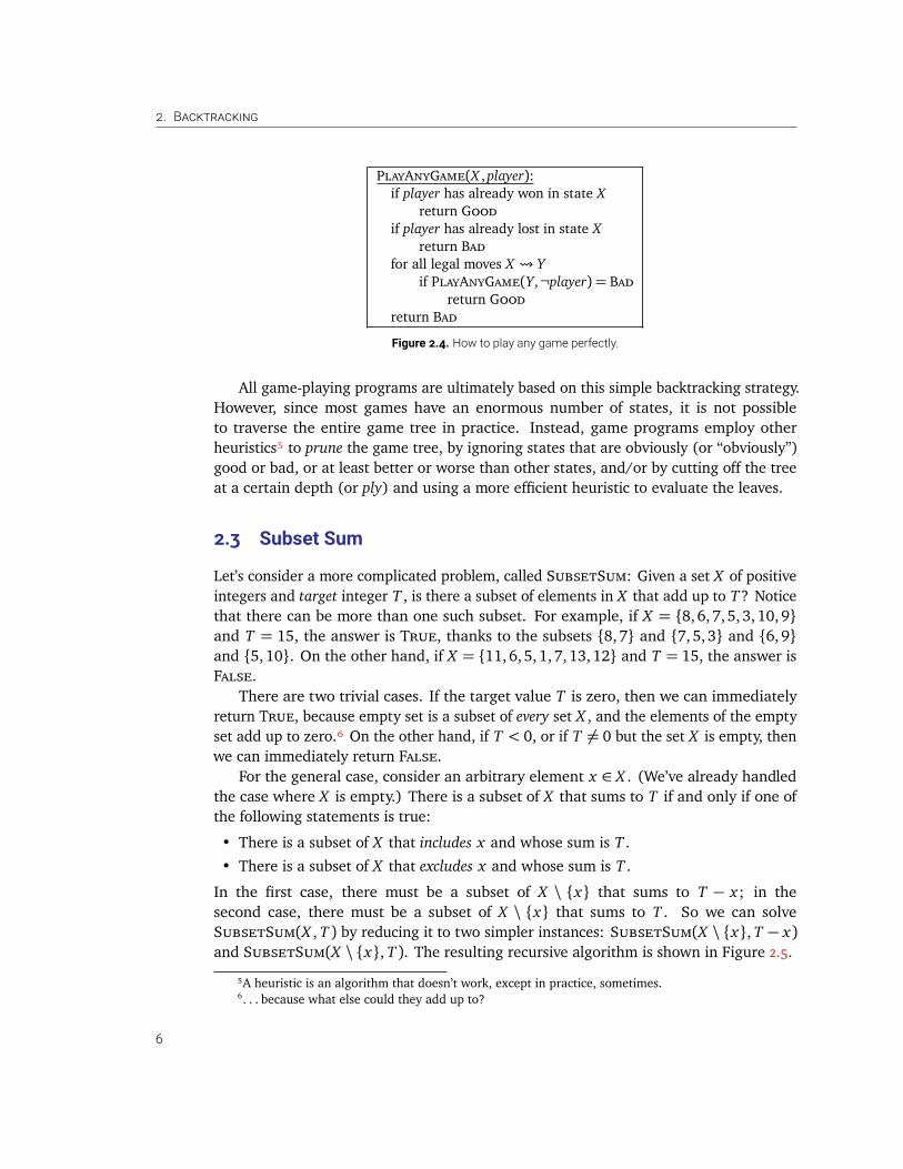
PlayAnyGame(X ,player):if player has already won in state X

return Goodif player has already lost in state X

return Badfor all legal moves X Y

if PlayAnyGame(Y,¬player) = Badreturn Good

return Bad

Figure 2.4. How to play any game perfectly.

All game-playing programs are ultimately based on this simple backtracking strategy.However, since most games have an enormous number of states, it is not possibleto traverse the entire game tree in practice. Instead, game programs employ otherheuristics⁵ to prune the game tree, by ignoring states that are obviously (or “obviously”)good or bad, or at least better or worse than other states, and/or by cutting off the treeat a certain depth (or ply) and using a more efficient heuristic to evaluate the leaves.

2.3 Subset Sum

Let’s consider a more complicated problem, called SubsetSum: Given a set X of positiveintegers and target integer T , is there a subset of elements in X that add up to T? Noticethat there can be more than one such subset. For example, if X = 8, 6,7,5, 3,10, 9and T = 15, the answer is True, thanks to the subsets 8,7 and 7, 5,3 and 6,9and 5,10. On the other hand, if X = 11,6, 5,1, 7,13, 12 and T = 15, the answer isFalse.

There are two trivial cases. If the target value T is zero, then we can immediatelyreturn True, because empty set is a subset of every set X , and the elements of the emptyset add up to zero.⁶ On the other hand, if T < 0, or if T 6= 0 but the set X is empty, thenwe can immediately return False.

For the general case, consider an arbitrary element x ∈ X . (We’ve already handledthe case where X is empty.) There is a subset of X that sums to T if and only if one ofthe following statements is true:

• There is a subset of X that includes x and whose sum is T .

• There is a subset of X that excludes x and whose sum is T .

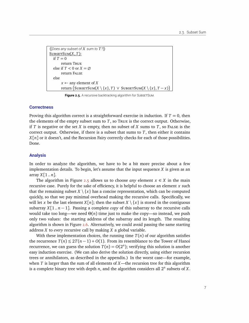
In the first case, there must be a subset of X \ x that sums to T − x; in thesecond case, there must be a subset of X \ x that sums to T . So we can solveSubsetSum(X , T ) by reducing it to two simpler instances: SubsetSum(X \ x, T − x)and SubsetSum(X \ x, T ). The resulting recursive algorithm is shown in Figure 2.5.

5A heuristic is an algorithm that doesn’t work, except in practice, sometimes.6. . . because what else could they add up to?

6

2.3. Subset Sum

⟨⟨Does any subset of X sum to T?⟩⟩SubsetSum(X , T ):if T = 0

return Trueelse if T < 0 or X =∅

return Falseelse

x ← any element of Xreturn

SubsetSum(X \ x, T ) ∨ SubsetSum(X \ x, T − x)

Figure 2.5. A recursive backtracking algorithm for SUBSETSUM.

Correctness

Proving this algorithm correct is a straightforward exercise in induction. If T = 0, thenthe elements of the empty subset sum to T , so True is the correct output. Otherwise,if T is negative or the set X is empty, then no subset of X sums to T , so False is thecorrect output. Otherwise, if there is a subset that sums to T , then either it containsX [n] or it doesn’t, and the Recursion Fairy correctly checks for each of those possibilities.Done.

Analysis

In order to analyze the algorithm, we have to be a bit more precise about a fewimplementation details. To begin, let’s assume that the input sequence X is given as anarray X [1 .. n].

The algorithm in Figure 2.5 allows us to choose any element x ∈ X in the mainrecursive case. Purely for the sake of efficiency, it is helpful to choose an element x suchthat the remaining subset X \ x has a concise representation, which can be computedquickly, so that we pay minimal overhead making the recursive calls. Specifically, wewill let x be the last element X [n]; then the subset X \ x is stored in the contiguoussubarray X [1 .. n− 1]. Passing a complete copy of this subarray to the recursive callswould take too long—we need Θ(n) time just to make the copy—so instead, we pushonly two values: the starting address of the subarray and its length. The resultingalgorithm is shown in Figure 2.6. Alternatively, we could avoid passing the same startingaddress X to every recursive call by making X a global variable.

With these implementation choices, the running time T (n) of our algorithm satisfiesthe recurrence T (n) ≤ 2T (n− 1) +O(1). From its resemblance to the Tower of Hanoirecurrence, we can guess the solution T (n) = O(2n); verifying this solution is anothereasy induction exercise. (We can also derive the solution directly, using either recursiontrees or annihilators, as described in the appendix.) In the worst case—for example,when T is larger than the sum of all elements of X—the recursion tree for this algorithmis a complete binary tree with depth n, and the algorithm considers all 2n subsets of X .

7

2. BACKTRACKING

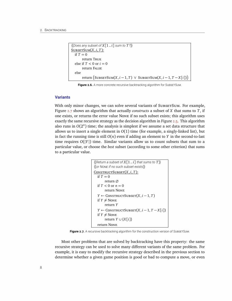
⟨⟨Does any subset of X [1 .. i] sum to T?⟩⟩SubsetSum(X , i, T ):if T = 0

return Trueelse if T < 0 or i = 0

return Falseelse

return

SubsetSum(X , i − 1, T ) ∨ SubsetSum(X , i − 1, T − X [i])

Figure 2.6. A more concrete recursive backtracking algorithm for SUBSETSUM.

Variants

With only minor changes, we can solve several variants of SubsetSum. For example,Figure 2.7 shows an algorithm that actually constructs a subset of X that sums to T , ifone exists, or returns the error value None if no such subset exists; this algorithm usesexactly the same recursive strategy as the decision algorithm in Figure 2.5. This algorithmalso runs in O(2n) time; the analysis is simplest if we assume a set data structure thatallows us to insert a single element in O(1) time (for example, a singly-linked list), butin fact the running time is still O(n) even if adding an element to Y in the second-to-lasttime requires O(|Y |) time. Similar variants allow us to count subsets that sum to aparticular value, or choose the best subset (according to some other criterion) that sumsto a particular value.

⟨⟨Return a subset of X [1 .. i] that sums to T ⟩⟩⟨⟨or NONE if no such subset exists⟩⟩ConstructSubset(X , i, T ):if T = 0

return ∅if T < 0 or n= 0

return NoneY ← ConstructSubset(X , i − 1, T )if Y 6= None

return YY ← ConstructSubset(X , i − 1, T − X [i])if Y 6= None

return Y ∪ X [i]return None

Figure 2.7. A recursive backtracking algorithm for the construction version of SUBSETSUM.

Most other problems that are solved by backtracking have this property: the samerecursive strategy can be used to solve many different variants of the same problem. Forexample, it is easy to modify the recursive strategy described in the previous section todetermine whether a given game position is good or bad to compute a move, or even

8

2.4. The General Pattern

the best possible move. For this reason, when we design backtracking algorithms, weshould aim for the simplest possible variant of the problem, computing a number or evena single bit instead of more complex information or structure.

2.4 The General Pattern

Backtracking algorithms are commonly used to make a sequence of decisions, with thegoal of building a recursively defined structure satisfying certain constraints; often thisgoal structure is itself a sequence. For example:

• In the n-queens problem, the goal is a sequence of queen positions, one in each row,such that no two queens attack each other. For each row, the algorithm decides whereto place the queen.

• In the game tree problem, the goal is a sequence of legal moves, such that each moveis as good as possible for the player making it. For each game state, the algorithmdecides the best possible next move.

• In the subset sum problem, the goal is a sequence of input elements that have aparticular sum. For each input element, the algorithm decides whether to include itin the output sequence or not.

(Hang on, why is the goal of subset sum finding a sequence? That was a deliberate designdecision. We impose a convenient ordering on the input set—by representing it using anarray as opposed to some other more amorphous data structure—that we can exploit inour recursive algorithm.)

In each recursive call to the backtracking algorithm, we need to make exactly onedecision, and our choice must be consistent with all previous decisions. Thus, eachrecursive call requires not only the portion of the input data we have not yet processed,but also a suitable summary of the decisions we have already made. For the same ofefficiency, the summary of past decisions should be as small as possible. For example:

• For the n-queens problem, we must pass in not only the number of empty rows, butthe positions of all previously placed queens. We have no choice but to rememberour past decisions in complete detail.

• For the game tree problem, we only need to pass in the current state of the game,including the identity of the next player. We don’t need to remember anything aboutour past decisions, because who wins from a given game state does not depend onthe moves that created that state.⁷

• For the subset sum problem, we need to pass in both the remaining available integersand the remaining target value, which is the original target value minus the sum of

7This requirement is not satisfied by all games. For example, the standard rules of chess allow a playerto declare a draw if the same arrangement of pieces occurs three times, and the Chinese rules for go simplyforbid repeating any earlier arrangement of stones. Thus, for these games, a game state formally includesthe entire history of previous moves.

9

2. BACKTRACKING

the previously chosen elements. Precisely which elements were previously chosen isunimportant.

When we design new recursive backtracking algorithms, we must figure out in advancewhat information we will need about past decisions in the middle of the algorithm. If thisinformation is nontrivial, our recursive algorithm must solve a more general problemthan the one we were originally asked to solve. (We’ve seen this kind of generalizationbefore: To find the median of an unsorted array in linear time, we derived an algorithmto find the kth smallest element for arbitrary k.)

2.5 Longest Increasing Subsequence

For any sequence S, a subsequence of S is another sequence from S obtained by deletingzero or more elements, without changing the order of the remaining elements; theelements of the subsequence need not be together in the original sequence S. Forexample, when you drive down a major street in any city, you drive through a sequenceof intersections with traffic lights, but you only have to stop at a subsequence of thoseintersections, where the traffic lights are red. If you’re very lucky, you never stop at all:the empty sequence is a subsequence of S. On the other hand, if you’re very unlucky,you may have to stop at every intersection: S is a subsequence of itself.

As another example, the strings BENT, ACKACK, SQUARING, and SUBSEQUENT are allsubsequences of the string SUBSEQUENCEBACKTRACKING, as are the empty string andthe entire string SUBSEQUENCEBACKTRACKING, but the strings QUEUE and DIMAGGIO arenot. A subsequence whose elements are contiguous in the original sequence is called asubstring; for example, MASHER and LAUGHTER are both subsequences of MANSLAUGHTER,but only LAUGHTER is a substring.

Now suppose we are given a sequence of integers, and we need to find the longestsubsequence whose elements are in increasing order. More concretely, the input is aninteger array A[1 .. n], and we need to compute the longest possible sequence of indices1≤ i1 < i2 < · · ·< i` ≤ n such that A[ik]< A[ik+1] for all k.

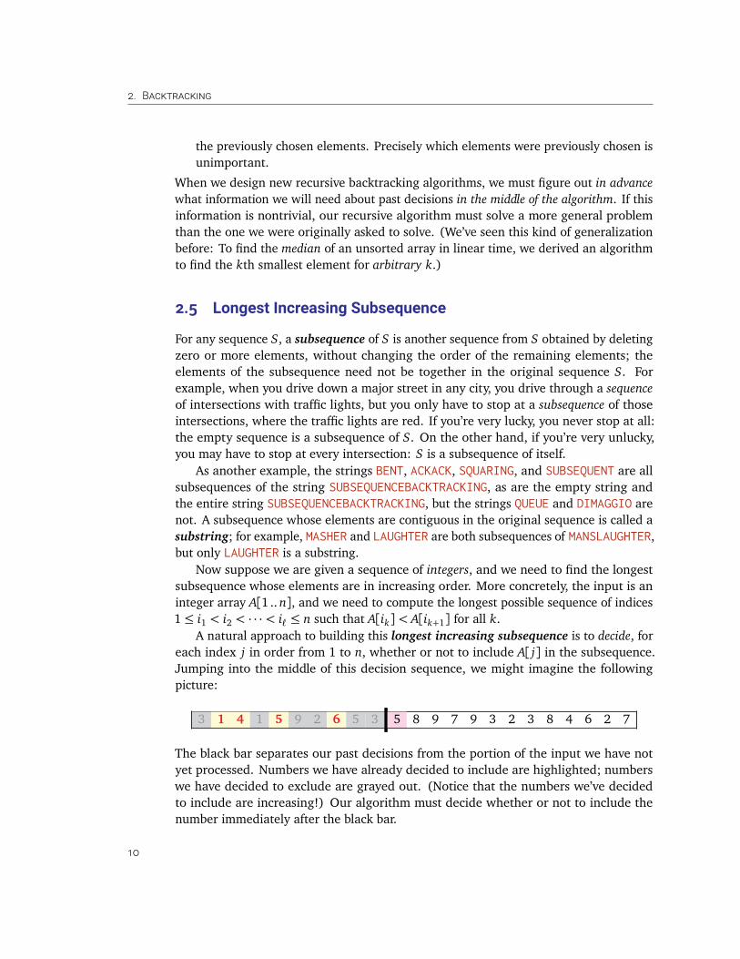
A natural approach to building this longest increasing subsequence is to decide, foreach index j in order from 1 to n, whether or not to include A[ j] in the subsequence.Jumping into the middle of this decision sequence, we might imagine the followingpicture:

3 1 4 1 5 9 2 6 5 3 5 8 9 7 9 3 2 3 8 4 6 2 7

The black bar separates our past decisions from the portion of the input we have notyet processed. Numbers we have already decided to include are highlighted; numberswe have decided to exclude are grayed out. (Notice that the numbers we’ve decidedto include are increasing!) Our algorithm must decide whether or not to include thenumber immediately after the black bar.

10

2.5. Longest Increasing Subsequence

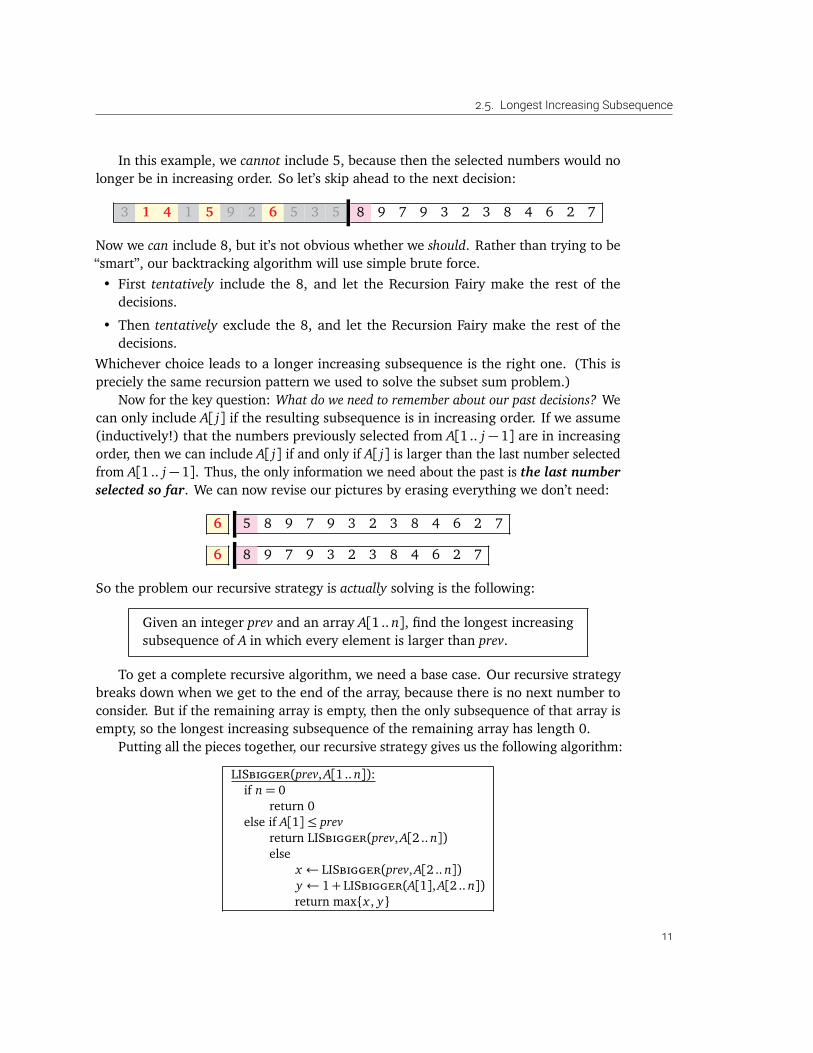
In this example, we cannot include 5, because then the selected numbers would nolonger be in increasing order. So let’s skip ahead to the next decision:

3 1 4 1 5 9 2 6 5 3 5 8 9 7 9 3 2 3 8 4 6 2 7

Now we can include 8, but it’s not obvious whether we should. Rather than trying to be“smart”, our backtracking algorithm will use simple brute force.• First tentatively include the 8, and let the Recursion Fairy make the rest of the

decisions.

• Then tentatively exclude the 8, and let the Recursion Fairy make the rest of thedecisions.

Whichever choice leads to a longer increasing subsequence is the right one. (This ispreciely the same recursion pattern we used to solve the subset sum problem.)

Now for the key question: What do we need to remember about our past decisions? Wecan only include A[ j] if the resulting subsequence is in increasing order. If we assume(inductively!) that the numbers previously selected from A[1 .. j − 1] are in increasingorder, then we can include A[ j] if and only if A[ j] is larger than the last number selectedfrom A[1 .. j − 1]. Thus, the only information we need about the past is the last numberselected so far. We can now revise our pictures by erasing everything we don’t need:

6 5 8 9 7 9 3 2 3 8 4 6 2 7

6 8 9 7 9 3 2 3 8 4 6 2 7

So the problem our recursive strategy is actually solving is the following:

Given an integer prev and an array A[1 .. n], find the longest increasingsubsequence of A in which every element is larger than prev.

To get a complete recursive algorithm, we need a base case. Our recursive strategybreaks down when we get to the end of the array, because there is no next number toconsider. But if the remaining array is empty, then the only subsequence of that array isempty, so the longest increasing subsequence of the remaining array has length 0.

Putting all the pieces together, our recursive strategy gives us the following algorithm:

LISbigger(prev, A[1 .. n]):if n= 0

return 0else if A[1]≤ prev

return LISbigger(prev, A[2 .. n])else

x ← LISbigger(prev, A[2 .. n])y ← 1+ LISbigger(A[1], A[2 .. n])return maxx , y

11

2. BACKTRACKING

Finally, we need to connect our recursive strategy to the original problem: Findingthe longest increasing subsequence of an array with no other constraints. The simplestapproach is to use an artificial sentinel value −∞:

LIS(A[1 .. n]):return LISbigger(−∞, A[1 .. n])

Assuming we can pass around the arrays in constant time, the running time of thisalgorithm satisfies the recurrence T (n)≤ 2T (n− 1) +O(1), which as usual implies thatT (n) = O(2n). We really shouldn’t be surprised by this running time; in the worst case,the algorithm examines each of the 2n subsequences of the input array.

Index Formulation

In practice, passing arrays as input parameters to algorithm is rather slow; we shouldreally find a more compact way to describe our recursive subproblems. for purposes ofdesigning the algorithm, it’s often useful to treat the original input array A[1 .. n] as aglobal variable⁸ and then reformulate the problem we’re trying to solve in terms of arrayindices instead of explicit subarrays.

For our longest increasing subsequence problem, the integer prev is typically an arrayelement A[i], and the remaining array is always a suffix A[ j .. n] of the original inputarray. So we can reformulate our recursive problem as follows:

Given two indices i and j, where i < j, find the longest increasingsubsequence of A[ j .. n] in which every element is larger than A[i].

Let LIS(i, j) denote the length of the longest increasing subsequence of A[ j .. n] with allelements larger than A[i]. Our recursive strategy gives us the following recurrence:

LIS(i, j) =

0 if j > n

LIS(i, j + 1) if A[i]≥ A[ j]maxLIS(i, j + 1), 1+ LIS( j, j + 1) otherwise

To solve the original problem, we can add a sentinel value A[0] = −∞ to the input array,and then recursively compute LIS(0, 1) following the recurrence above.

This is precisely the same algorithm as LISbigger; the only thing we’ve changedis notation. However, using index notation instead of array notation will be importantwhen we start discussing dynamic programming in the next chapter.

ÆÆÆ Alternative strategy: Let LIS(i)denote the length of the longest increasing subsequenceof A[i .. n] that begins with A[i]. If we set A[0] = −∞, then we want LIS(0)− 1. In fact,this is how longest increasing subsequences are computed in O(n log n) time.8In practice, we would more likely pass a pointer/reference to the original input array as another

parameter of our recursive subroutine.

12

2.6. Optimal Binary Search Trees

2.6 Optimal Binary Search Trees

Our final example combines recursive backtracking with the divide-and-conquer strategy.Recall that the running time for a successful search in a binary search tree is proportionalto the number of ancestors of the target node.⁹ As a result, the worst-case search time isproportional to the depth of the tree. Thus, to minimize the worst-case search time, theheight of the tree should be as small as possible; by this metric, the ideal tree is perfectlybalanced.

In many applications of binary search trees, however, it is more important to minimizethe total cost of several searches rather than the worst-case cost of a single search. If xis a more frequent search target than y , we can save time by building a tree where thedepth of x is smaller than the depth of y , even if that means increasing the overall depthof the tree. A perfectly balanced tree is not the best choice if some items are significantlymore popular than others. In fact, a totally unbalanced tree with depth Ω(n) mightactually be the best choice!

This situation suggests the following problem. Suppose we are given a sorted arrayof keys A[1 .. n] and an array of corresponding access frequencies f [1 .. n]. Our task isto build the binary search tree that minimizes the total search time, assuming that therewill be exactly f [i] searches for each key A[i].

Before we think about how to solve this problem, we should first come up with agood recursive definition of the function we are trying to optimize! Suppose we are alsogiven a binary search tree T with n nodes. Let vi denote the node that stores A[i], andlet r be the index of the root node. Then ignoring constant factors, the total cost ofperforming all the binary searches is given by the following expression:

Cost(T, f [1 .. n]) =n∑

i=1

f [i] ·#ancestors of vi in T (∗)

The root vr is an ancestor of every node in the tree. If i < r, then all ancestors of vi inthe left subtree; similarly, if i > r, all other ancestors of vi are in the right subtree. Thus,we can partition the cost function into three parts as follows:

Cost(T, f [1 .. n]) =n∑

i=1

f [i] +r−1∑

i=1

f [i] ·#ancestors of vi in left(T )

+n∑

i=r+1

f [i] ·#ancestors of vi in right(T )

9An ancestor of a node v is either the node itself or an ancestor of the parent of v. A proper ancestorof v is either the parent of v or a proper ancestor of the parent of v.

13

2. BACKTRACKING

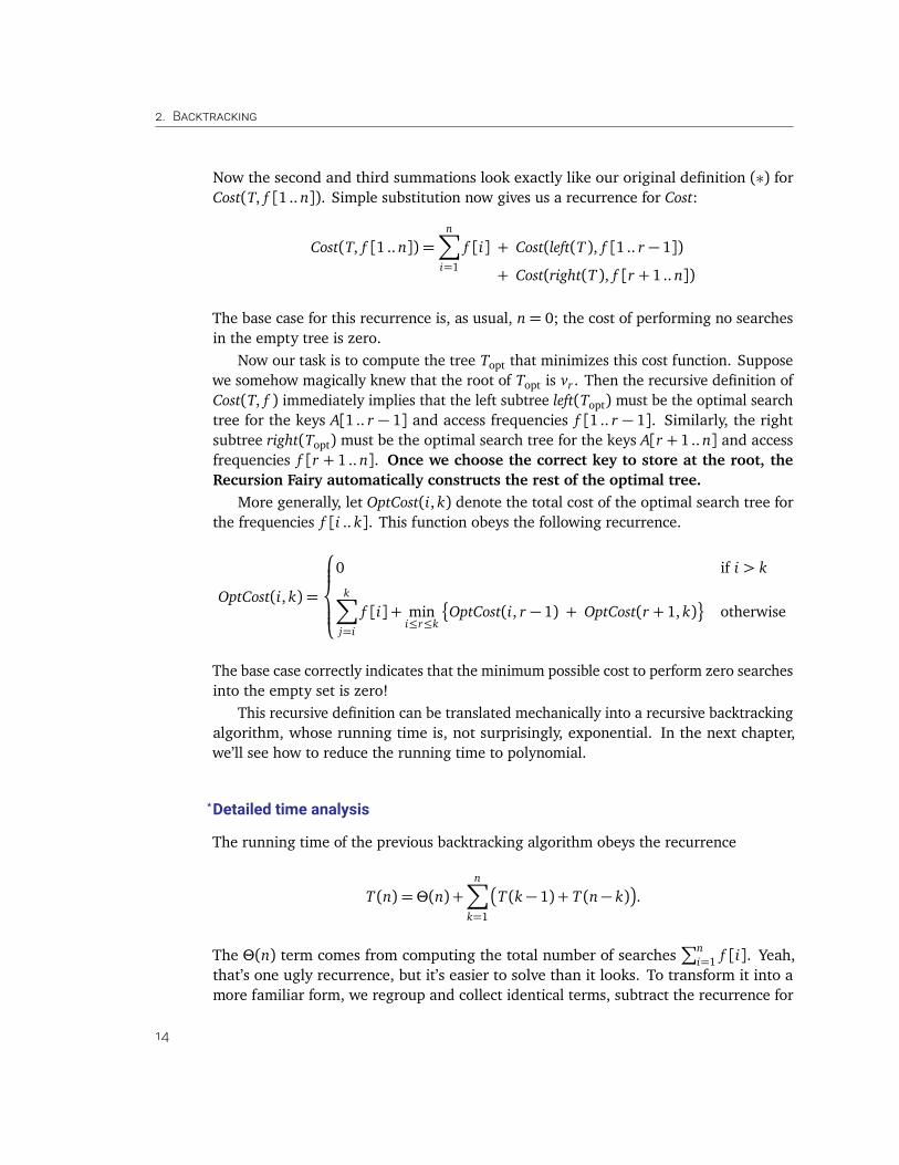
Now the second and third summations look exactly like our original definition (∗) forCost(T, f [1 .. n]). Simple substitution now gives us a recurrence for Cost:

Cost(T, f [1 .. n]) =n∑

i=1

f [i] + Cost(left(T ), f [1 .. r − 1])

+ Cost(right(T ), f [r + 1 .. n])

The base case for this recurrence is, as usual, n= 0; the cost of performing no searchesin the empty tree is zero.

Now our task is to compute the tree Topt that minimizes this cost function. Supposewe somehow magically knew that the root of Topt is vr . Then the recursive definition ofCost(T, f ) immediately implies that the left subtree left(Topt) must be the optimal searchtree for the keys A[1 .. r − 1] and access frequencies f [1 .. r − 1]. Similarly, the rightsubtree right(Topt) must be the optimal search tree for the keys A[r + 1 .. n] and accessfrequencies f [r + 1 .. n]. Once we choose the correct key to store at the root, theRecursion Fairy automatically constructs the rest of the optimal tree.

More generally, let OptCost(i, k) denote the total cost of the optimal search tree forthe frequencies f [i .. k]. This function obeys the following recurrence.

OptCost(i, k) =

0 if i > k

k∑

j=i

f [i] + mini≤r≤k

OptCost(i, r − 1) + OptCost(r + 1, k)

otherwise

The base case correctly indicates that the minimum possible cost to perform zero searchesinto the empty set is zero!

This recursive definition can be translated mechanically into a recursive backtrackingalgorithm, whose running time is, not surprisingly, exponential. In the next chapter,we’ll see how to reduce the running time to polynomial.

?Detailed time analysis

The running time of the previous backtracking algorithm obeys the recurrence

T (n) = Θ(n) +n∑

k=1

T (k− 1) + T (n− k)

.

The Θ(n) term comes from computing the total number of searches∑n

i=1 f [i]. Yeah,that’s one ugly recurrence, but it’s easier to solve than it looks. To transform it into amore familiar form, we regroup and collect identical terms, subtract the recurrence for

14

Exercises

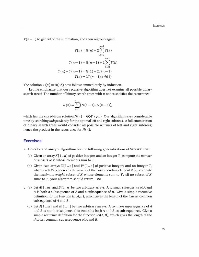
T (n− 1) to get rid of the summation, and then regroup again.

T (n) = Θ(n) + 2n−1∑

k=0

T (k)

T (n− 1) = Θ(n− 1) + 2n−2∑

k=0

T (k)

T (n)− T (n− 1) = Θ(1) + 2T (n− 1)

T (n) = 3T (n− 1) +Θ(1)

The solution T(n) = Θ(3n) now follows immediately by induction.Let me emphasize that our recursive algorithm does not examine all possible binary

search trees! The number of binary search trees with n nodes satisfies the recurrence

N(n) =n−1∑

r=1

N(r − 1) · N(n− r)

,

which has the closed-from solution N(n) = Θ(4n/p

n). Our algorithm saves considerabletime by searching independently for the optimal left and right subtrees. A full enumerationof binary search trees would consider all possible pairings of left and right subtrees;hence the product in the recurrence for N(n).

Exercises

1. Describe and analyze algorithms for the following generalizations of SubsetSum:

(a) Given an array X [1 .. n] of positive integers and an integer T , compute the numberof subsets of X whose elements sum to T .

(b) Given two arrays X [1 .. n] and W [1 .. n] of positive integers and an integer T ,where each W [i] denotes the weight of the corresponding element X [i], computethe maximum weight subset of X whose elements sum to T . sIf no subset of Xsums to T , your algorithm should return −∞.

2. (a) Let A[1 .. m] and B[1 .. n] be two arbitrary arrays. A common subsequence of A andB is both a subsequence of A and a subsequence of B. Give a simple recursivedefinition for the function lcs(A, B), which gives the length of the longest commonsubsequence of A and B.

(b) Let A[1 .. m] and B[1 .. n] be two arbitrary arrays. A common supersequence of Aand B is another sequence that contains both A and B as subsequences. Give asimple recursive definition for the function scs(A, B), which gives the length of theshortest common supersequence of A and B.

15

2. BACKTRACKING

(c) Call a sequence X [1 .. n] oscillating if X [i] < X [i + 1] for all even i, and X [i] >X [i + 1] for all odd i. Give a simple recursive definition for the function los(A),which gives the length of the longest oscillating subsequence of an arbitrary arrayA of integers.

(d) Give a simple recursive definition for the function sos(A), which gives the lengthof the shortest oscillating supersequence of an arbitrary array A of integers.

(e) Call a sequence X [1 .. n] accelerating if 2 ·X [i]< X [i−1]+X [i+1] for all i. Givea simple recursive definition for the function lxs(A), which gives the length of thelongest accelerating subsequence of an arbitrary array A of integers.

For more backtracking exercises, see the next chapter!

© Copyright 2016 Jeff Erickson.This work is licensed under a Creative Commons License (http://creativecommons.org/licenses/by-nc-sa/4.0/).Free distribution is strongly encouraged; commercial distribution is expressly forbidden.See http://jeffe.cs.illinois.edu/teaching/algorithms/ for the most recent revision.16