Department of Economics Working Paper

Bad Government Can Be Good Politics: Political Reputation, Negative Campaigning, and Strategic

Shirking

Deborah Fletcher Miami University

Steven Slutsky

University of Florida

February 2009

Working Paper # - 2009-01

*We would like to thank James Foster and David Sappington for their helpful comments. An earlier version of this paper was presented at the Third World Congress of the Game Theory Society in 2008.

Bad Government Can Be Good Politics: Political Reputation, Negative Campaigning,

and Strategic Shirking*

by

Deborah Fletcher Department of Economics

208 Laws Hall Miami University

Oxford, OH 45056

and

Steven Slutsky Department of Economics

Matherly Hall University of Florida

Gainesville, FL 32611  

February 2009

Abstract: We develop a model of a contest between two political candidates who may care about their reputations separately from how they affect the election outcome. In the game’s first stage, each candidate chooses to maintain his maximum reputation or to shirk to lower it. In the second stage, candidates undertake positive or negative campaigns. We allow the magnitudes of reputational effects of positive and negative campaigns, and the relative importance candidates place on reputation and winning, to vary. Under many parameter values, candidates shirk in order to change the equilibrium strategies and outcome in the second stage of the game.

 

  2

 “Good government is good politics.” 

                                                                                                                           Mayor Richard J. Daley 

I. Introduction

Whether politicians shirk has been extensively studied as a type of principal-agent problem:

the agent-politician has different interests from the principal-voters and acts in accordance with

the voters' interests only if disciplined at the ballot box. One branch of that literature has studied

whether term-limited politicians in their final term behave differently than when reelection is

possible1. Even when reelection is possible, a representative may shirk to get large campaign

contributions or direct transfers of wealth.2 In these cases, good government remains good

politics: a politician who shirks gives up political advantage for personal gain.

In this paper, we demonstrate an alternative possibility: political shirking, instead of being

minimized by the electoral process, can be caused by strategic factors arising from that process

even when politicians and voters have common preferences. To establish this, we develop a

simple stylized model of a political contest between an incumbent and a challenger.

Candidates begin the contest with initial reputations that are then altered by campaign

activities. Initial reputations could be based on many factors including policy positions,

competence in governing, and personal attributes, some of which can be affected by the

candidates, at least in a downward direction. The incumbent might intentionally choose a

reputation below the maximum by being inefficient or by adopting unpopular policies. The

challenging party might run a candidate whose reputation is lower than some other potential

challenger’s, since all the potential challengers will not start with the same reputations. In the

first initial reputation stage, candidates may choose their initial reputations simultaneously or

sequentially.

In the second campaign stage, candidates simultaneously choose whether to run positive or

negative campaigns. A candidate raises his own reputation by running a positive campaign, and

lowers the opponent’s reputation by running a negative campaign. If both run negative

campaigns, both lose reputation but by an amount that may be larger or smaller than the loss

from running a positive campaign against the opponent’s negative one. At the end of the

1 See Bender and Lott (1996) for a review of the political shirking literature. Later treatments of this topic include, among others, Schmidt et al (1996), Figlio (2000), Rothenberg and Sanders (2000) and Lawrence (2007). 2 See Chappell (1981) and Bender (1991).

  3

campaign, the winner of the election is the candidate with the higher reputation. The winning

candidate values the sum of her reputation and a bonus from winning. The loser values his post-

election reputation.

Some assumptions about voter and candidate preferences are crucial to the analysis. We

treat the electorate as a single representative voter. In effect, all voters view the candidates

identically rather than having different preferences. One justification for this approach is that

Downsian convergence has occurred, so that both candidates advocate the same policies. All

voters would then prefer the candidate who is more competent.

Candidate preferences depend on reputation both because reputations affect the outcome of

the contest and because candidates value reputation directly.3 One pole would be politicians

who follow the famous precept attributed to Vince Lombardi: “Winning isn’t everything; it’s the

only thing.” These candidates would care only about winning the election. The opposite pole

would be “gentlemen politicians” who behave according to the Grantland Rice adage: “It’s not

that you won or lost, but how you played the game,” and care only about reputation independent

of the election’s outcome. We consider how the equilibrium varies as different importance is

given to these two factors when candidates are between the two poles.4

For many parameter values, in the first stage, one candidate engages in a type of shirking by

selecting an initial reputation lower than the maximum feasible value. Such strategic shirking

occurs because having a lower reputation yields a more advantageous second stage equilibrium

for the candidate. In particular, with a reduced initial reputation, a candidate is often less likely

3 Placing a value on reputation need not be altruistic. It might be for long-term gain, such as to increase future political or commercial success. This could take a number of forms. For example, Francis et al (1994) explore how politicians’ past policy decisions affect their probability of achieving a higher elected office, while Parker (2003) considers whether reputational capital can limit shirking by politicians. 4 Varying the bonus to be larger or smaller than other reputational factors is formally equivalent to candidates valuing a weighted sum of those factors and the bonus and varying the weights. A substantial literature explores the impact of different objective functions for political candidates. Most of this literature has focused on the differences between maximizing expected vote share and maximizing the probability of winning. Aranson, Hinich and Ordeshook (1974), Ledyard (1984), Snyder (1989), Duggan (2000) and Patty (2005) have considered the relation between outcomes under these two objectives. Politicians with policy preferences as well as preferences for the election outcome were considered by Wittman (1973). The distinction between the utility a candidate would get from winning the election and other reputational factors has not been previously considered. Since all voters in our model are identical, maximizing vote share and probability of winning would be equivalent candidate objectives. Unlike the setting with policy preferences, voters and candidates have the same preferences for candidate reputations in our setting.

  4

to be the target of a negative campaign by the opponent. Bad government, to some extent and in

some circumstances, can be good politics.

A simple example illustrates this possibility. Consider an election between a challenger

and an incumbent who start with equal reputations of 30. Before the actual campaign begins, the

incumbent must vote either for or against some measure. Voting for it will raise the incumbent’s

reputation to 40 in the eyes of the voters while voting against it will lower the incumbent’s

reputation to 20. Both the voters and the incumbent himself prefer that he have the highest

possible reputation, so it would seem straightforward that the incumbent would vote yes.

However, a campaign will take place after the incumbent’s action on the measure and

before the election. In the campaign, each candidate may run either a positive campaign or a

negative campaign. A positive campaign raises the candidate’s own reputation by 7. Negative

campaigns are very effective, so a negative campaign lowers the opponent’s reputation by 20 if

the opponent runs a positive campaign. If both run negative campaigns, the voters are angered by

the negative campaign war, and each candidate’s reputation drops by 25. The candidate who

wins the election gets a boost to reputation of 10.

What happens if the incumbent votes for, rather than against, the measure? Since the

incumbent has the larger initial reputation, he loses the election only if he runs a positive

campaign against the opponent’s negative one, as this combination reduces his reputation by 13

and leaves the challenger’s reputation unchanged. The payoff matrix for the campaign stage is

then:

C

Even though the incumbent loses when he goes positive against the challenger’s negative

campaign, this is better for him than going negative, since the reputation loss of 25 from the

campaign war is larger than the bonus from winning of 10. Thus, when starting with the higher

P N

P

N I

57, 37 27, 40

50, 17 25, 5

  5

reputation, the incumbent has a dominant strategy of going positive in the campaign game. The

challenger goes negative and wins the election. The incumbent ends with a reputation of 27.

If instead, the incumbent voted against the measure and began the campaign stage with

the reduced reputation, the incumbent would win only when going negative against the

challenger’s positive campaign. The campaign game payoff matrix is now the following:

C

In every box, the incumbent is worse off than when voting yes. However, it is the

challenger now who has the dominant strategy of going positive. In equilibrium, the incumbent

goes negative and wins the election, ending with a reputation of 30. The incumbent ends up

gaining by voting against the preferences of the voters in the first stage.

This example is sufficient to show that strategic shirking can be politically beneficial. A

more general analysis is needed to determine how typical is this behavior --- when does such

shirking occur? Additionally, it will help us to understand why such shirking can be beneficial --

- is it always so that in the campaign stage the shirker goes negative instead of positive and wins

the election? The rest of the paper presents this general analysis.

Related literature is discussed in Section II. The model is described in Section III. Second

stage equilibria for all possible parameter values are presented in Section IV, and first stage

equilibria are derived in Section V. Extensions and conclusions are discussed in Section VI.

II. Related Literature

We are not the first to suggest the possibility of gains from actions that appear to be self-

destructive. In the game theory literature, it has been argued that players can gain by sacrificing

resources or “burning money” (see, for example Ben-Porath and Dekel (1992) and Van Damme

(1989)). In that literature, the self-sacrifice is a way for a player to signal what action will be

taken in a later stage of the game, and is used as a method of equilibrium selection based on

forward induction. Often, what matters is that burning money is possible, but this action is not

P N

P

N I

27, 47 7, 40

30, 17 -5, 15

  6

chosen in equilibrium. In our model, the reduction in reputation is not done to select among

multiple equilibria or to signal future actions. Instead, it alters the nature of the second stage

equilibrium, which may well be unique.

In the political context, Hess and Orphanides (1995) show that elections may induce

shirking instead of preventing it, a result similar to ours. An incumbent in her first term may

enter an avoidable war (shirk) in order to enhance her reputation and improve her chance of re-

election. A term-limited incumbent in the final term never does this. Although reputation is

crucial in both our framework and theirs, the logic behind the results is very different. In their

model, shirking raises reputation and this increases the chances of winning the election. In our

model, shirking always reduces reputation, but a lower reputation can enhance a candidate’s

electoral chances by changing the equilibrium in the campaign stage.

Hodler, Loertscher and Rohner (2007) also develop a model in which incumbents can gain

electoral advantage by selecting inefficient policies. Their model is based upon asymmetric

information between incumbents and voters. The incumbent chooses inefficient policies that

change voter beliefs in a way that improves his odds of re-election. Our model has no

information asymmetries, with the results based on strategic interactions between the candidates.

In the industrial organization literature, a related thread shows that a firm or agent may gain

by intentionally harming itself for one of two reasons: the action harms a rival more than it

harms the initiator, or rivals are not directly harmed but are induced to take actions benefiting the

initiator. Examples of the first, where self-sabotage --- analogous to shirking --- directly harms

the rival, are Williamson (1968) and Sappington and Weisman (2005). Williamson shows that a

firm may increase its own costs by agreeing to a high-wage union contract that binds not only

itself but also rivals that are harmed even more by the higher wages. Sappington-Weisman show

that a vertically integrated producer supplying itself and rivals downstream may gain by reducing

the quality of those inputs, if the competitors suffer a greater harm.

The second reason occurs in Gelman and Salop (1983), in which an entrant can gain by

limiting capacity if it then becomes so small that the incumbent does not seek to force it out of

the market by undercutting its price. Shirking directly benefits the opponent, but is undertaken

because it leads to a more advantageous outcome later in the game. In Bose, Pal, and Sappington

(2008), an agent intentionally increases total production costs while reducing marginal cost to

  7

induce the principal to offer a more attractive compensation scheme. In some situations, a Pareto

improvement results from the agent’s sabotage.

Our result is more akin to the second reason: shirking by a candidate with no other change

may actually increase the opponent’s probability of being elected. It is nevertheless undertaken

because it brings about a new second stage equilibrium that is more advantageous to the shirker.

Our argument is somewhat more complex than in the literature discussed above, since shirking

does not simply affect the opponent’s actions, but induces a new equilibrium where both players

may adjust their behavior. For example, there exist situations where the candidate entering the

second stage with the higher reputation runs a positive campaign against the opponent’s negative

one and loses the election. By shirking, the situation is reversed, and the shirker now goes

negative against an opponent’s positive campaign and wins.

The interaction between first stage reputation and second stage negative campaigning is

crucial to generating equilibrium shirking. The emphasis by pundits and campaign managers on

the importance of negative campaigning in determining the outcomes of elections is consistent

with its importance in our model. Surprisingly, there have been few formal models of negative

campaigning. One model by Skaperdas and Grofman (1995) assumes that there are initially

three types of voters: partisans of each candidate and undecided voters. Through positive

campaigning, a candidate shifts initially undecided voters into supporters. By negative

campaigning, a candidate shifts some opponent partisans into the undecided category. However,

due to a boomerang effect, some of the candidate’s own partisans become undecided.

Harrington and Hess (1996) develop a model of negative campaigning in which voters

evaluate candidates in terms of issue positions and personal traits. Voters differ in their

preferences over the former, but agree in their evaluation of the latter. Campaigning affects

voters’ views only on the policy dimension. A candidate who runs positive ads is perceived to

have issue positions more compatible with the preferences of swing voters while after running

negative ads, the opponent’s position is perceived to be further away from the preferences of

swing voters. As in Skaperdas-Grofman, candidates maximize expected vote share and make a

continuous decision between positive and negative campaigning. In both models there is a single

type of equilibrium. One result in Harrington-Hess is that a candidate preferred on the personal

dimension runs a relatively positive campaign, while the opponent runs a relatively negative one.

  8

In some ways, our model is simpler than those discussed above. In our model, candidates

differ only in reputation, which corresponds to the personal traits. We do not include a

boomerang effect, have only a single representative voter rather than three types or a continuum,

and assume that candidates make a discrete decision over a positive or negative campaign rather

than a continuous one.5 These simplifications allow us to add the complication that the

effectiveness of a candidate’s negative campaign can depend on whether the opponent chooses a

positive or negative campaign. We also allow candidates to care about more than the electoral

outcome. Finally, the above papers only have a single stage, which is equivalent to the second

stage of our two-stage model. In our game, the initial reputation in the second stage is

endogenous, where the factors analogous to reputation are exogenously determined in the papers

discussed above. These additional complications mean that instead of there being only one type

of equilibrium, as in Skaperdas-Grofman and Harrington-Hess, different types of equilibria exist

at different parameter values in our model. This is crucial for the existence of strategic shirking.

III. The Model

a. The Campaign Game

The game between an incumbent I and a challenger C takes place in two stages. In the first

stage, the initial reputations of the candidates are determined. For the incumbent, this is largely

based upon the way the incumbent governs. Governing in the best manner possible for that

individual would attain for the incumbent some maximum value of reputation. Deviating from

this by choosing policies the voters do not want, by implementing policies inefficiently, or by

engaging in personal scandals would reduce the incumbent’s initial reputation below the

maximum value. The incumbent’s initial reputation is denoted by X, and the range it can take by

the interval [XL, XU]. For the challenger, initial reputation is denoted as Y, and is based upon

5 While a continuous decision might seem more realistic, modeling negative campaigning as a discrete choice might be more appropriate under some circumstances. A candidate running a single negative ad could be viewed as running a negative campaign if that ad received a significant amount of media attention. For example, the famed Swift Boat ads of the 2004 Presidential election ran only a few times. Similarly, the Daisy ad by Lyndon B. Johnson in the 1964 campaign only ran once. In these cases, using the fraction of ads that were negative would grossly underestimate the extent to which the campaign was viewed as negative.

  9

which individual the party not in power decides to select as its nominee. We assume that there is

a range of possible candidates the party can choose from, denoted by the interval [YL, YU].6

Different timings of when the two candidates choose their initial reputations are possible.

The most realistic is that the incumbent, having been in office, selects a reputation first and then

the challenger chooses a reputation knowing what the incumbent has done. However, the

incumbent may be able to take actions late in the term of office after the challenger has been

selected to alter this initial reputation, especially in a downward direction. Thus, it may be

possible to have a game in which the incumbent moves second. We also consider a simultaneous

move game, although this may be harder to justify in reality.

The second stage is the actual campaign. After the candidates observe the initial reputations

each has chosen in the first stage, perhaps by polling voters, they each must decide whether to

run a positive or a negative campaign, where these choices are denoted as P and N. If a

candidate runs a positive campaign, this raises that candidate’s reputation by an amount G. If a

candidate runs a negative campaign, this lowers the opponent’s reputation by an amount L,

provided the opponent runs a positive campaign. However, if both run negative campaigns, then

each reputation is reduced by an amount D.7 Assuming the candidates must make a discrete

choice of running either a positive or negative campaign, then the post-campaign reputation

matrix is shown below, with the incumbent’s reputation shown as the first term in each cell8:

6 We treat reputation as a choice variable in the first stage. In actuality, these reputations are determined by other choices about policy or personal behavior. However, since we assume voters are identical in their preferences and the effect of these policies is through reputation, we can treat reputation as the choice variable without any loss.

7 For simplicity, we assume that G, L and D are independent of the candidates’ initial reputations. More realistically, these parameters might differ between the incumbent or the challenger, or between the winner and loser of the race. However, adding these complications would not change the general nature of the results. We discuss the effects of some of these modifications in the conclusion section. 8 This is not the payoff matrix in the second stage since the bonus is not included in each box. Who wins varies with the specific parameter values.

C

P N

P

N I

X + G, Y + G X + G – L, Y

X, Y + G – L X – D, Y – D

  10

Two relations among the parameters G, L, and D are significant in the analysis of the

second stage equilibria: how L compares to G and how D compares to L – G. Having L greater

than G would impose the commonly believed proposition that negative campaigning is

particularly effective. This means not just that a negative campaign lowers the opponent’s

reputation (L positive) but that a negative campaign lowers the opponent’s reputation more than

a positive campaign would raise the candidate’s own reputation.9 If G were greater than or equal

to L, there would be no advantage to a candidate from running a negative campaign.10

The second comparison relates to what has been called meltdown, where both candidates run

negative campaigns. The resulting voter alienation has two different manifestations with very

different implications for the outcome. One is that the voters are angry with the candidates for

mudslinging, greatly lowering the reputations of both, making D greater than L. Alternatively,

voters are disillusioned by the campaign, become apathetic, and pay little attention to it. Largely

ignored, negative ads become less effective, leading D to be less than L. What turns out to be

crucial to the results is whether this voter apathy is extreme, occurring to such an extent that D is

less than or equal to L – G. 11 A candidate concerned about the effect of an opponent’s negative

ads on his reputation could run positive ads to directly restore reputation or could run negative

ads to make voters apathetic about the campaign and thereby make the opponent’s negative ads

less effective. When D is small relative to L – G, the second strategy is the more effective one.

The candidates are assumed to choose their strategies simultaneously in the second stage

game. Whether either candidate would have the opportunity to move first might depend upon

when the challenger is chosen. If primaries are close to the final election, potential challengers

9 The relative effectiveness of negative and positive campaign ads has been the subject of significant debate. Authors including Lau (1982, 1985), Basil, Schooler, and Reeves (1991) and Newhagen and Reeves (1991) have suggested that voters are more likely to remember negative information about political candidates than positive information. However, a review and meta-analysis performed by Lau et al (1999) suggests there is no strong evidence that negative ads are more effective than positive ones. 10 A “boomerang” effect, where a candidate running a negative campaign also loses reputation, would reinforce this. Candidates would then run negative campaigns only if L were significantly larger than G. Boomerang effects are discussed in Garramone (1984) and Merritt (1984), and play an important role in the negative campaigning model of Skaperdas and Grofman (1995). Assuming them here would complicate our analysis but not change the essential nature of the results. 11 The empirical evidence about meltdown is sparse and gives mixed results. Mayer (1996) quotes a Congressional Research Service report and several popular press articles that suggest negative campaign wars alienate voters, although Mayer himself defends the use of negative advertising. There has also been a debate about whether negative campaign wars decrease participation, which could be a signal that such wars cause voter apathy. This debate began with Ansolabehere and Iyengar’s (1995) contention that negative campaigns depress participation, but several other authors have found that negative campaigns actually increase turnout. See Brooks (2006) for a discussion of this debate.

  11

might begin negative attacks on the incumbent even before a specific individual is chosen to be

the actual opposing candidate. The incumbent might have to wait until after the primary to know

which individual to attack. On the other hand, if the primary is a relatively long time before the

general election, attacking the incumbent so early might be counterproductive. In this case, the

incumbent and challenger would be in a symmetric situation and would make their strategic

decisions on the type of campaign to run simultaneously.

b. Election Outcome and Voter Preferences

When individuals decide for whom to vote, their only concern is the candidates’ post-

campaign reputations. Thus, in any of the boxes in the matrix in (1), the candidate with the

higher reputation wins. If both candidates play the same strategy, so that either (P, P) or (N, N)

results, then the winner is the candidate with the higher initial reputation since the campaign

affects them equally. I wins if X > Y and C wins if the reverse holds. If X = Y, we assume that

each has an equal chance of winning. If I chooses P and C chooses N, similarly, the outcome

depends on whether X + G – L – Y is positive, negative, or zero while if I chooses N and C

chooses P, the outcome depends on whether Y + G – L – X is positive, negative, or zero.

c. Candidate Preferences

The goal of each candidate is to maximize his reputation. In addition to the post-campaign

reputation, the winning candidate gets a boost to reputation denoted B. When the post-campaign

reputations are the same, the candidates are equally likely to win. We assume risk neutrality so

that, ex ante, each gets an expected boost of B/2. There are a number of reasons why candidates

care about their reputations and not just winning. A winning candidate may be able to achieve

more in office when starting with a higher reputation. A losing candidate may intend to run

again for that or some other office in the future, and a higher reputation coming out of this

campaign will affect success in future campaigns. In addition, prospects out of office for losing

candidates or retiring incumbents may depend upon their reputations. Varying the size of B

relative to the direct effects of campaign activities on reputation allows the candidates to have

preferences that, in effect, vary between the polar cases of gentleman politicians and

Lombardians. The objective of maximizing reputation will approach that of being concerned

only with winning if B is large relative to G, L, and D. If B is smaller than these, even

approaching zero, then the gentleman politician polar case is approached.

  12

Note that candidate and voter preferences have a large element of agreement in that both

value candidate reputations. The candidates do not directly gain by reducing their own

reputations as might occur in a principal-agent model, where reducing effort increases the

agent’s leisure. There might seem to be one aspect of disagreement in that the candidates also

care about the bonus B from winning, which does not appear to enter voter preferences.

However, if the voters were assumed to care about the post-election reputation of the winner, this

would not alter their behavior. The bonus B would be a constant awarded to whomever they

selected and would not affect their choice among the candidates.

d. Solution Concept

The game tree when the incumbent moves first in the initial stage and the candidates make

their decisions simultaneously in the second stage is shown in Figure 1. Given the sequential

nature of the game, we consider the equilibria to be the subgame perfect Nash equilibria. In

particular, when choosing initial reputations in the first stage, the candidates look ahead to how

these will affect the outcomes in the second stage campaign. Hence, as is standard, we will solve

the game backwards, first computing the second stage equilibria conditional on the initial

reputations and then finding the equilibrium choice of initial reputations in the first stage.

Due to multiple second stage equilibria and discontinuities in first stage payoffs, we need

several additional assumptions to specify the equilibria. First, when the multiple second stage

equilibria are Pareto ranked so that both candidates agree on which is best, we assume that the

Pareto preferred equilibrium is the one selected by the candidates. Second, when the multiple

second stage equilibria are not Pareto ranked, we assume that the candidates have a common

belief in the form of a probability distribution over the equilibria. Taking the expected value of

the payoffs given this distribution specifies their expected payoffs in this situation. Third, due to

discontinuities in the first stage payoffs found from backwards induction, when reputations are

chosen sequentially in the first stage, a best reply may not exist for one of the candidates. When

this happens, there is a choice for that candidate that gives her a payoff arbitrarily close to the

supremum. In such cases, we assume that the outcomes are described by ε-equilibria.12

IV. Second Stage Equilibria

12 Radner (1980) developed the notion of ε-equilibria in the context of firms playing a finitely repeated Cournot game. An ε-equilibrium requires that each player’s strategy yields a payoff within ε of the maximum possible against the other player’s equilibrium strategies.

  13

The equilibria in the second stage subgame depend on the reputations chosen in the first

stage only in how those reputations (X and Y) affect which candidate wins the election under

different choices of positive and negative campaigns (P and N) by the candidates. In fact, these

reputations affect the election outcomes only through their difference X – Y. In Lemmas 1, 2,

and 3, we specify the second stage equilibria for all parameter values. Lemma 1 considers the

case where negative campaigning is relatively ineffective.

Lemma 1: When L ≤ G, the unique equilibrium at all values of X and Y is (P, P).

When X < Y, UI = X + G and UC = Y + G + B; when X = Y, UI = X + G + B/2 and UC = Y + G

+ B/2; and when X > Y, UI = X + G + B and UC = Y + G.

That is, when negative campaigning is less effective than positive campaigning, positive

campaigns strictly dominate. Not only will a candidate not choose a negative campaign as a pure

strategy, but there will also be no mixed strategies with a positive probability of negative

campaigning in equilibrium. A positive campaign directly raises a candidate’s reputation, and

also gives the candidate at least as good a chance of winning the election as a negative campaign.

Lemmas 2 and 3 consider the cases where L is greater than G. The seven possible ranges in

which X – Y could fall are shown in Figure 2. Note that as X increases from 0, X – Y moves in

order through all seven regions as shown by the arrow in the Figure. The regions are as follows:

(1) X – Y < G – L with C winning for all choices of second stage strategies, (2) X – Y = G – L

with the candidates tying when I chooses N and C chooses P and with C winning in the other

three cases, (3) G – L < X – Y < 0 with I winning under the strategies (N, P) and C winning in

the other three cases, (4) X – Y = 0 with I winning under (N, P), C winning under (P, N), and

their tying in the remaining two cases, (5) 0 < X – Y < L – G with C winning under (P, N) and I

winning in the other three cases, (6) X – Y = L – G with I winning in all cases except (P, N)

where a tie occurs, and finally, (7) L – G < X – Y with I winning in all cases. Regions (1), (3),

(5), and (7) are interior regions in that in each of them X – Y can take a range of values. Regions

(2), (4), and (6) are boundary regions in that in each of them X – Y must take a particular value.

The equilibria for ranges (5), (6), and (7) are not stated since I and C differ only in the values of

their initial reputations. Since the game is otherwise symmetric, the equilibria in ranges (5), (6),

and (7) are identical to those in ranges (3), (2), and (1), respectively, reversing the names of the

  14

candidates and their strategies. When mixed strategy equilibria exist, p and q denote the

probabilities with which I and C respectively run positive campaigns.

Lemma 2 considers the case when a candidate’s own reputation is higher when responding

to an opponent’s negative campaign with a negative rather than a positive campaign.

Lemma 2: When D < L – G, (N, N) is an equilibrium at all values of the other parameters

with UI = X – D and UC = Y – D + B in regions (1), (2), and (3) and with UI = X – D + B/2 and

UC = Y – D + B/2 in region (4). In addition,

(a) (P, P) is also an equilibrium in region (1) if G < B/2

(b) (P, P) is also an equilibrium in regions (1), (2), and (4), if B/2 < G < B,

(c) (P, P) is also an equilibrium in regions (1), (2), (3), and (4) if B < G.

The payoffs for (P, P) in the different regions are the same as in Lemma 1 above. When both

(P, P) and (N, N) are equilibria, there is also a mixed strategy equilibrium with payoffs for each

player in between those for the pure strategy equilibria. When multiple equilibria exist, they are

Pareto ranked, with both candidates preferring (P, P) to the mixed strategy equilibrium, which is

preferred to (N, N). When the equilibria relate in this fashion, it is reasonable to assume that,

when contemplating setting reputations so that X – Y would fall into a region with multiple

equilibria, either candidate would assume that the Pareto optimal equilibrium (P, P) would be the

one selected in the second stage.

The importance of winning relative to direct reputation (how B and B/2 compare to G)

determines whether (N, N) is a unique equilibrium or whether (P, P) is also an equilibrium in

regions (2), (3), and (4). The smaller is B relative to G (that is, the more gentlemanly are the

politicians), the larger is the number of regions with multiple equilibria. When G is less than B,

(N, N) is the unique equilibrium in the interior regions (3) and (5), and when G is less than B/2,

it is also the unique equilibrium in boundary regions (2) and (4). Thus, when candidates have

preferences near the Lombardian pole, both candidates go negative in the second stage

equilibrium, except in regions (1) and (7). When candidate preferences are near the opposite

pole, the candidates always choose positive campaigns in the second stage equilibrium.

Finally, in Lemma 3 we consider the case where negative campaigning is relatively effective

but the harm from meltdown is sufficiently large that, when the opponent goes negative, a

positive campaign in response gives the candidate a higher reputation than does a negative one.

  15

Lemma 3: When D > L – G > 0, the equilibrium strategies and payoffs in the seven regions are:

(1) (P, P) with UI = X + G and UC = Y + G + B

(2) (a) If G > B/2, (P, P) with UI = X + G and UC = Y + G + B

(b) If G < B/2 < D + G – L, (N, P) with UI = X + B/2 and UC = Y + G – L + B/2

(c) If B/2 > max [G, D + G – L], [(P, N, p), (P, N, q)] where p =

(B/2 + L – G – D)/(B/2 + L – D) and q = (D + G – L)/(B/2 + D – L) with UI =

X + G – L(B/2 – G)/( B/2 + D – L) and UC = Y + G + B – G(B/2 + L)/( B + L – D)

(3) (a) If G < B < D + G – L, (N, P) with UI = X + B and UC = Y + G – L

(b) If B > max [G, D + G – L], [(P, N, p), (P, N, q)] where p = 1 – G/(B + L – D) and q =

(D + G – L)/(B + D – L) with UI = X + G – L(B – G)/( B + D – L) and UC =

Y + G + B – G(B + L)/( B + L – D)

(c) If B < G, (P, P) with UI = X + G + B/2 and UC = Y + G + B/2

(4) (a) If B/2 < min [G, D + G – L], (P, P) with UI = X + G + B/2 and UC = Y + G + B/2

(b) If D + G – L < B/2 < G, (P, P) with UI = X + G + B/2 and UC = Y + G + B/2, (N, N)

with UI = X – D + B/2 and UC = Y – D + B/2, and [(P, N, p), (P, N, q)] where p = q =

1 – (G – B/2)/(L – D) with UI = X + G + B/2 – (G – B/2)/(B/2 + L)/(L – D) and UC =

Y + G + B/2 – (G – B/2)(B/2 + L)/(L – D)

(c) If G < B/2 < D + G – L, (N, P) with UI = X + B and UC = Y + G –L, (P, N) with

UI = X + G - L and UC = Y + B, and [(P, N, p), (P, N, q)] where p = q =

1 – (B/2 – G)/(D – L) with UI = X + G + B/2 – (B/2 – G)(B/2 + L)/(D – L) and UC =

Y + G + B/2 – (B/2 – G)(B/2 + L)/(D – L)

(d) If B/2 > max [G, D + G – L], (N, N) with UI = X + B/2 – D and UC = Y + B/2 – D

In all regions except (1) and (7), subcases exist depending upon whether either B or B/2 is

greater or less than G or D + G – L. Only in subcases 4(b) and 4(c), in which X = Y and B/2 lies

between G and D + G – L, do multiple equilibria exist. 4(b) arises when D < L, and 4(c) when D

> L. The multiple equilibria in these two subcases are very different. The multiple equilibria in

4(b) are the same as those in Lemma 2, and so can be Pareto ranked, with the (P, P) equilibrium

preferred. In 4(c), however, the equilibria cannot be Pareto ranked. The candidates have

opposite rankings, with I preferring (N, P) to (P, N) and C preferring the reverse, and both

ranking the mixed strategy equilibrium in between. Since X = Y in this subcase and the mixed

  16

strategy equilibrium is symmetric, the candidates receive the same expected payoff in it. Overall,

the expected payoffs across the three equilibria, given the common beliefs of the candidates, lie

in a range between their values when (N, P) and (P, N) are the equilibria. Parameter values exist

making the mixed strategy payoff near the upper and lower end of the range. Because of this, the

expected payoffs of the candidates could be selected independently of each other.

In the other subcases, there is a unique equilibrium, which can either be in pure strategies or

in mixed strategies. In subcases 2(c) and 3(b) the unique equilibrium is in mixed strategies; note

that in both of these subcases, B can be relatively large (and thus the candidates can be near the

Lombardian pole). In these mixed strategy equilibria, both candidates run negative ads with

some probability greater than zero. Depending on the specific parameter values in each subcase,

the probability of a candidate running a negative campaign can be anywhere between 0 and 1 and

either candidate could have the higher probability of going negative.

Among the unique pure strategy equilibria, only in 4(d) --- which again has B large --- do

both candidates choose negative campaigns. (P, P) is the unique pure strategy equilibrium either

when B is small (subcases 2(a), 3(c) and 4(a) and the symmetric subcases 6(a) and 5(c)), or when

the difference between X and Y is large (regions (1) and (7)). The candidates will both choose

positive campaigns when other reputational effects are very important relative to the bonus from

winning, or when one candidate has a large reputational advantage at the beginning of the second

stage. When B has intermediate values, in the cases with pure strategy equilibria (subcases 2(b)

and 3(a)), one candidate will choose a negative campaign and the other will choose a positive

campaign in equilibrium.

Based upon the parameter restrictions in the three lemmas, six qualitatively different

scenarios exist which are mutually exclusive and which exhaust the parameter space.13 These

six scenarios are described below, with Figures 3 to 8 showing a representative graph of the

equilibrium utilities as functions of X and Y for each of them. The restrictions defining each

scenario are written as bounds on G, the reputation gain from running a positive ad. G has a key

role in specifying these conditions because a candidate is always able to take an action that gains

13 That there are not more scenarios follows from a number of reasons. One is that subcases in one region may not occur with subcases in another region. For example, in Lemma 3, subcase 3(a) is not consistent with 2(c), 4(b), or 4(d). Another is that some of the subcases differ in their full sets of Nash equilibria but after equilibrium selection such as taking the Pareto preferred equilibria, they are identical. This is true for subcases 4(a) and 4(b) of Lemma 3.

  17

that candidate G independently of the other candidate’s actions. The other parameters B, L, and

D are reputation changes that depend on the actions of the other candidate. Note that, as shown

in Figure 3, the game is symmetric between the two candidates. Thus, only the incumbent’s

graph is shown in Figures 4 – 8.

(i) min [B, L] ≤ G [Lemma 1 or Lemma 2(c), or Lemma 3 subcases 2(a), 3(c), and 4(a) or 4(b)]

Either negative campaigning is ineffective or the candidates value reputation more than

winning. This scenario includes the polar case of gentlemen politicians. As shown in

Figure 3, each candidate’s utility is strictly increasing in the candidate’s reputation.

(ii) max [B/2, B + L – D] < G < min [B, L] [Lemma 3 subcases 2(a), 3(a), and 4(a)]

Negative campaigning is effective, voters become angry at the candidates if both go

negative, and candidate preferences are relatively gentlemanly, putting significant weight on

reputation beyond winning. As shown in Figure 4, for X ≤ Y, UI is strictly increasing in X,

then at X > Y it decreases discontinuously and is always below the value at X = Y until X =

Y + L – G, where it jumps above.

(iii) B/2 < G < min [B, L, B + L – D] [Lemma 2(b) or Lemma 3 subcases 2(a), 3(b), and 4(a) or

4(b)]

Negative campaigning is effective, meltdown could be of either type, and the candidates are

intermediate between the two polar cases. As shown in Figure 5, for X ≤ Y + G – L, UI is

continuous and strictly increasing, then it decreases discontinuously for X above Y + G – L.

It then increases linearly for X < Y, with its peak as X approaches Y being above or below

the value at Y + G – L. It increases discontinuously at X = Y, then decreases discontinuously

for X greater than Y. It again increases linearly for X above Y. Its value as X approaches Y

+ L – G may be above or below the value at X = Y. Finally, it increases discontinuously

again at X = Y + L – G.

(iv) max [0, B + L – D] < G < min [B/2, L] [Lemma 3 subcases 2(b), 3(a), and 4(c)]

Negative campaigning is effective, voters become extremely angry at the candidates if both

go negative, and candidate preferences are intermediate but may lean toward the Lombardian

pole, putting significant weight on the bonus from winning. As shown in Figure 6, UI is

strictly increasing in X for X < Y. At X = Y + ε, UI is strictly below its value at Y - ε. At X =

Y, there are multiple equilibria, where the best one closes UI from below and the worst closes

it from above. The expected payoffs across the multiple equilibria must lie between

  18

these limits.

(v) max [0, B/2 + L – D] < G < min [B/2, L, B + L – D] [2(b), 3(b), and 4(c) of Lemma 3]

Negative campaigning is effective, voters become angry if there is a negative campaign war,

and candidate preferences are between the poles, but tend toward the Lombardian pole.

There exist many ambiguities in specifying the graph of payoffs in this scenario due to

ambiguities in the comparison of the payoffs in the different regions (for example, either of

the region 3 and 5 lines could be above the other) as well as multiple possibilities for

expected payoffs when X = Y. The best and worst values there can be above and below the

nearby values in the neighboring interior regions. In region (2), UI is above the limiting value

in region (1) and it is also below the value in region (6). Figure 7 shows one representative

possibility for the graph of UI.

(vi) 0 < G < min [B/2, L, B/2 + L – D] [2(c), 3(b), and 4(d) of Lemma 3 or Lemma 2(a)]

Negative campaigning is effective, neither form of meltdown is either implied or ruled out,

and the candidates strongly value winning. The Lombardian pole is included in this scenario.

As shown in Figure 8, the graph of UI is strictly increasing in X for Y ≤ X. For X < Y, it

decreases discontinuously around X = Y + G – L with the value at Y + G – L lying between

the limiting values as X approaches Y + G – L from above and below.

Scenario (i), which contains the gentleman candidate polar case, always arises under

sufficiently large G regardless of the values of the other parameters. For any particular values of

B, L, and D some of the other scenarios will not arise at any G, since the conditions needed for

those scenarios cannot be satisfied at the particular parameter values. As G declines, there is a

tendency to move in order through those scenarios that can exist. The space of parameters B, L,

and D can be partitioned into three regions: (a) 0 < B/2 < D – L, (b) 0 < D – L < B/2, and (c) D –

L < 0. Under (a), scenarios (iii) and (vi) can never occur and as G gets smaller, the scenario

shifts from (i) to (ii) to (iv) to (v). Under (b), the shift is from scenario (i) to (ii) to (iii) to (v) to

(vi) while under (c) it is from (i) to (iii) to (vi). When L < B, additional scenarios may no longer

exist with the shift across scenarios as G changes continuing in order through the remaining

ones.

In scenario (i), utilities are strictly increasing in reputation. In the other five scenarios, they

are discontinuous, globally nonmonotonic, and are not quasiconcave. Utilities within a single

  19

interior region rise monotonically with reputation, but can have a discontinuous drop when

moving from one region to the next due to differences in the second stage equilibria in different

regions. As seen in the next section, these properties create the possibility that candidates can

benefit by reducing their own reputations in the first stage; that is, they can benefit from shirking.

V. First Stage Equilibria

Since the game is symmetric between the candidates except for differences in XU and YU

and between XL and YL, only cases where XU – YU > 0 will be considered14. For XU – YU < 0,

the outcomes are the same as for XU – YU > 0 with I and C reversed. This means that any

equilibrium given for C moving first can also be interpreted as the equilibrium when the

incumbent moves first but has a lower reputation than the challenger.

In the appendices, the formal specifications of the equilibria for each scenario are stated in

six theorems and their proofs. In the text, we present a series of propositions giving the intuition

behind these results. First, Propositions 1 and 2 give conditions under which neither candidate

shirks.

Proposition 1: Assume that at least one of the following parameter restrictions is satisfied:

A. positive campaigning is at least as effective as negative campaigning;

B. candidates are close to the gentleman politician pole, gaining at least as much in

reputation from running a positive campaign as from the winning bonus;

C. the difference in their maximum possible initial reputations is greater than the difference

between L and G.

Then, regardless of the timing by which initial reputations are selected, the unique subgame

perfect Nash equilibrium is that neither candidate shirks in the first stage, both candidates run

positive campaigns in the second stage, and the incumbent is reelected.

Proposition 1 is formally stated in Theorem 1. Conditions A and B correspond to

scenario (i). As shown in Figure 3, each candidate’s first stage utility is strictly increasing in the

candidate’s own initial reputation, causing each to have a dominant strategy of maximizing

14 Boundary situations, such as when XU – YU equals 0 or L – G or when B + L – D equals 0, are not considered. A variety of additional equilibria can sometimes arise in these situations that typically can be ruled out since one of the candidates is using a weakly dominated strategy. Otherwise, the equilibria are essentially the same as in the non-boundary cases.  

  20

initial reputation. Under condition C, XU – YU > L – G, so that in each of the remaining

scenarios the game is in region (7). In this region, candidate I always has a dominant strategy to

choose XU, and the challenger’s best reply is YU. This leads to the no-shirking outcome,

regardless of the timing of decisions in the first stage.

Proposition 2: Assume that all of the following conditions hold:

A. negative campaigning is more effective than positive campaigning;

B. the bonus from winning exceeds the reputation gain from running a positive campaign;

C. the difference in the maximum possible reputations of the candidates is less than L – G;

D. either (i) taking into account any response the opponent might make, the candidates do

not gain from lowering their initial reputations below their maximal levels, even given

the non-monotonicities in their utility functions or (ii)given the lower limits on their

initial reputations, candidates cannot lower their reputations sufficiently to take

advantage of any non-monotonicity.

Then, regardless of the timing by which initial reputations are selected, the unique subgame

perfect Nash equilibrium is that neither candidate shirks in the first stage. In the second

stage, depending on the parameter values, there are three possible outcomes: (a) the

incumbent may run a positive campaign against the challenger's negative campaign in the

second stage, and the challenger wins the election, (b) both run negative campaigns with the

incumbent winning, or (c) they both mix between running positive and negative campaigns and

each has some probability of winning the election.

Proposition 2 combines results in Theorem 2A, Theorem 3A, Theorem 4A(i), B(i), and C(i),

and Theorem 6A, which concern scenarios (ii), (iii), (iv), and (vi), respectively. It also includes

results from scenario (v), which we do not formally state. In scenario (ii), the challenger’s utility

is strictly increasing in Y when Y is below X, so the challenger would never gain by lowering

reputation. The incumbent’s utility in region (5) is always less than its value in region (4) with X

= Y, so the incumbent always desires to reduce reputation until it equals that of the challenger.

The no-shirking outcome occurs when XL is above YU, so that the incumbent is unable to reduce

his reputation enough to equal the challenger’s.

In scenario (vi), the incumbent would never gain from shirking, but the challenger might if

YU were close to XU + G – L. Thus, no shirking occurs if YL is above XU + G – L, or if YU is

  21

sufficiently above XU + G – L. In scenario (iii), similar restrictions must be placed on the

maximum and minimum values of the initial reputations of both candidates.

In scenario (iv), the conditions to rule out shirking depend on the timing of moves in the

first stage. When the challenger selects reputation first or the candidates select simultaneously,

the outcome is the same as in scenario (ii). However, when the incumbent moves first,

determining whether there is a gain from shirking requires considering the potential response by

the challenger. The incumbent would like to reduce X below YU but then the challenger would

respond by reducing Y below X, which could leave the incumbent worse off than initially. The

incumbent will not shirk if the possible reductions in reputation are too small to yield a benefit

(XL is not low enough) or if they allow for a harmful countermove by the challenger.

When the conditions of these two Propositions do not hold, different types of equilibria with

shirking exist. One of these, given in Proposition 3, is a type of coordination game equilibrium.

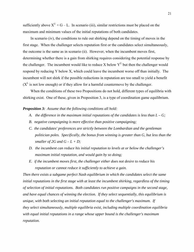
Proposition 3: Assume that the following conditions all hold:

A. the difference in the maximum initial reputations of the candidates is less than L – G;

B. negative campaigning is more effective than positive campaigning;

C. the candidates' preferences are strictly between the Lombardian and the gentleman

politician poles. Specifically, the bonus from winning is greater than G, but less than the

smaller of 2G and G – L + D;

D. the incumbent can reduce his initial reputation to levels at or below the challenger’s

maximum initial reputation, and would gain by so doing;

E. if the incumbent moves first, the challenger either does not desire to reduce his

reputation or cannot reduce it sufficiently to achieve a gain.

Then there exists a subgame perfect Nash equilibrium in which the candidates select the same

initial reputations in the first stage with at least the incumbent shirking, regardless of the timing

of selection of initial reputations. Both candidates run positive campaigns in the second stage,

and have equal chances of winning the election. If they select sequentially, this equilibrium is

unique, with both selecting an initial reputation equal to the challenger's maximum. If

they select simultaneously, multiple equilibria exist, including multiple coordination equilibria

with equal initial reputations in a range whose upper bound is the challenger's maximum

reputation.

  22

This Proposition covers scenarios (ii) and (iii), as given in Theorems 2 and 3B, and scenario

(v), which is not formally stated. In these equilibria, the candidates are better off having the

same reputations than for either to have a small reputational advantage. In scenarios (ii) and (iii),

when their reputations are the same, the candidates both run positive campaigns and have equal

chances of winning the election. In scenario (ii), when the reputations differ slightly the

disadvantaged candidate runs a negative campaign against the opponent’s positive one, and

although he always wins the election (instead of winning only half the time) the direct reputation

loss from not getting G with a positive campaign exceeds the gain of ½ B. In scenario (iii), both

candidates use mixed strategies when their reputations differ slightly, and the expected payoffs

can be less than when their reputations are the same. Finally, scenario (v) is more complex,

given the multiple equilibria when reputations are equal. If both candidates believe that the

mixed strategy equilibrium is highly likely and this gives both a high payoff, this coordination

game equilibrium can occur.

When reputations are chosen sequentially, both players choose a reputation of YU, so that

the incumbent shirks but the challenger does not. In scenario (ii), selecting YU is a dominant

strategy for the challenger. The only requirement this equilibrium, then, is that the incumbent is

able to reduce reputation to YU and desires to do so. In scenarios (iii) and (v), additional

conditions are needed to ensure that the challenger does not gain from shirking in response.

When the candidates select their initial reputations simultaneously, multiple equilibria exist.

In all but the boundary case where X = Y = YU, both candidates shirk. All of these coordination

equilibria are strict, but the one where they each choose reputations of YU is the Pareto superior

equilibrium among them. If the Pareto preferred selection criterion were imposed here, then just

as under sequential choice of initial reputation, only that equilibrium would be assumed to occur.

Such sequential choice could be viewed as one way in which the equilibrium selection is

achieved since each candidate would be willing to let the other select a reputation first.

A second type of equilibrium has only the challenger shirking. The conditions for this are

given in Proposition 4.

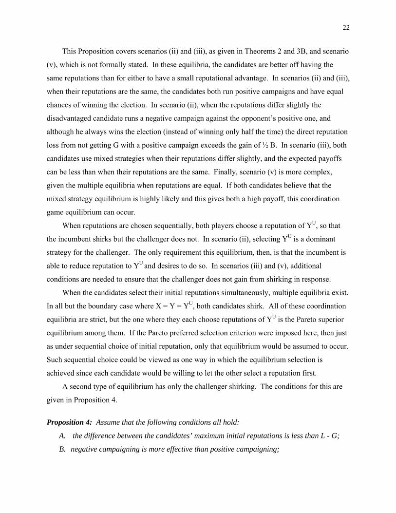
Proposition 4: Assume that the following conditions all hold:

A. the difference between the candidates’ maximum initial reputations is less than L - G;

B. negative campaigning is more effective than positive campaigning;

  23

C. the candidates' preferences are toward the Lombardian pole. Specifically, the bonus

from winning is greater than the larger of G and G – L + D;

D. the challenger gains by reducing reputation, taking into account the incumbent’s

response when the challenger moves first, and has sufficient flexibility to achieve that

gain;

E. the incumbent gains if the challenger reduces reputation, or the incumbent is unable to

block a reduction in reputation by the challenger via a reduction in his own reputation.

Then there exist subgame perfect Nash equilibria in which the incumbent chooses his maximal

reputation15, while the challenger reduces his reputation until it equals or is ε below XU + G - L.

Both candidates run positive campaigns in the second stage, and the incumbent always wins the

election.

This proposition encompasses scenarios (iii) and (vi), given in Theorems 3C and 6B, and

results from scenario (v). In all three of these scenarios, there are ranges of challenger

reputations above XU + G – L such that the challenger would benefit from reducing reputation to

either XU + G – L or to XU + G – L – ε when the incumbent’s reputation is fixed at XU. In

scenarios (iii) and (vi), such a move by the challenger yields the best possible outcome for the

incumbent. In scenario (vi), the incumbent never directly or indirectly benefits by reducing his

reputation, so if YU is in the specified range and YL is sufficiently low to allow the challenger’s

move, that will be an equilibrium independent of the order of moves. In scenario (iii), for XU

sufficiently close to YU, the incumbent would gain by shirking to YU, and such a move would

yield the best possible outcome for the challenger. Thus, if the challenger moves first, he might

refrain from shirking so that the incumbent, moving second, would. Therefore, for this to be an

equilibrium, XU must be sufficiently above YU so that the incumbent does not want to shirk to

YU, or XL must be above YU so that the incumbent is unable to shirk to YU. Given the

ambiguities in scenario (v), the incumbent may be made worse off when the challenger shirks,

and when moving first might block the challenger’s shirking by shirking himself. Condition E of

the Proposition rules out these possibilities, and is thus necessary only in scenario (v). For most

15 Note that this equilibrium need not be unique, as multiple equilibria sometimes exist. Under the parameter restrictions consistent with scenario (iii), when the candidates select reputations simultaneously, then the coordination equilibrium from Proposition 3 and the equilibrium where only the challenger shirks can exist simultaneously. 

  24

relevant parameter values, this equilibrium holds regardless of the order of moves, although in

some cases more stringent restrictions are needed when the incumbent moves first.

It is interesting to note that the challenger shirks even though this never increases his

probability of winning the election in the second stage, and may strictly reduce it. If neither

candidate shirks, the second stage equilibrium is either in mixed strategies, so that each would

have some chance of winning the election, or both undertake negative campaigns and the

incumbent always wins.16 After the challenger shirks, both run positive campaigns and the

challenger always loses. A non-pure Lombardian would prefer this outcome, since reputation is

important independent of the outcome of the election.

At first glance this seems puzzling, since scenario (vi), whose equilibria are treated in

Propositions 2 and 3, contains the Lombardian pole, where the candidates care only about

winning. The only two equilibria in this scenario are no shirking and having the challenger shirk

to move the second stage game to region (6). In the latter equilibrium, the challenger always

loses the election after shirking, but wins with some probability in the mixed strategy

equilibrium of region (5). However, as B gets large and winning becomes very important, the

probability of the challenger winning in the mixed strategy equilibrium goes to zero, apparently

at a faster rate than G/B. If reputation has any weight, however small, the challenger prefers to

avoid being the target of negative attacks.

In the previous four Propositions, the equilibria are essentially independent of the order of

moves in the first stage. In the equilibria given in Proposition 5, the first mover shirks and the

second mover does not, regardless of which candidate moves first.

Proposition 5: Assume that all of the following hold:

A. negative campaigning is more effective than positive campaigning;

B. the difference between the maximum initial reputations of the candidates is less than

either L – G or G;

C. the candidates' preferences are strictly between the Lombardian and the gentleman

politician poles. Specifically, G – L + D > B > 2G;

D. both candidates can reduce their initial reputations to levels at or below their

opponent’s maximum initial reputation less L – G. 16 The (N, N) equilibrium arises when B/2 < G < min [B, L – D]. 

  25

Then the unique subgame perfect Nash equilibrium is for the first mover to choose a reputation ε

below his opponent’s maximal reputation less L – G. Both candidates run positive campaigns in

the second stage, and the first mover always loses.

This proposition includes scenario (iv), as given in Theorem 4A(iii) and 4B(iv)17. The

results are based on who is the first mover rather than whether a candidate is an incumbent or a

challenger. If the candidates moved simultaneously and had sufficient downward flexibility in

their choice of reputation, a pure strategy equilibrium would not exist due to the desire of each to

undercut the other. 18

In scenario (iv), the first mover shirks sufficiently to move the equilibrium to regions (1) or

(7), at which point the second mover no longer wants to undercut and thus does not shirk. The

equilibrium is now (P, P), with the first mover losing, but avoiding a loss in reputation from the

negative campaign the opponent would have run if shirking had not occurred. When the

challenger is the first mover, this effect is indirect. If neither shirked, the challenger would have

run the negative campaign and would have won the election. After shirking, the election outcome

is switched with the incumbent winning. However, if the challenger had not shirked, the

incumbent would have been able to just undercut the challenger and the challenger would have

faced a negative campaign as well as an election loss. Similar behavior could occur in scenario

(v), where shirking moves the second stage equilibrium from mixed strategies to both running a

positive campaign.

There exists a mirror image of the equilibrium in Proposition 5, where instead of the first

mover, it is the second mover who shirks to the opponent’s maximum reputation less L – G. The

conditions for this are given in Proposition 6.

Proposition 6: Assume that all of the following hold:

A. negative campaigning is more effective than positive campaigning, and voters are

angered by a negative campaign war, so that D > L;

17 A similar equilibrium exists in scenario (v) but the exact parameter restrictions for it are complicated to state.

18 Dasgupta and Maskin (1986) and Reny (1999) give sufficient conditions for the existence of mixed strategy equilibria in games with discontinuous strategy spaces, as occurs in our first stage. Even if a mixed strategy equilibrium exists, the candidates would be placing positive probability on reputations below their maximums, and hence would be shirking with positive probability.

  26

B. the difference between the candidates’ maximum initial reputations is less than L – G;

C. the candidates' preferences are strictly between the Lombardian and the gentleman

politician poles. Specifically, the bonus from winning is greater than the larger of 2G

and G – L + D, but is smaller than 2(G – L + D);

D. Each candidate would gain by reducing reputation if the other did not, and both gain

more from the other’s reduction than from their own.

Then the unique subgame perfect Nash equilibrium is for the first mover to choose his maximum

possible reputation, and for the second mover to choose a reputation equal to his opponent’s

maximum less L – G. The first mover runs a positive campaign against the second mover’s

negative one, and the candidates have equal probabilities of winning the election.

This equilibrium can only occur in scenario (v); the conditions for it are presented in

Theorem 5. The equilibrium here has some similarity to that in Proposition 4, where the

challenger shirked to XU + G - L and the incumbent did not shirk. The difference is that the

equilibrium from Proposition 4 did not depend on the order of moves, whereas in this

equilibrium the challenger only shirks when moving second. In addition, this is the only case in

which an incumbent moving second chooses to reduce his reputation below that of the challenger

by more than an arbitrarily small ε.

The second mover runs a negative campaign after shirking, and wins the election half the

time. If not shirking, there would be a mixed strategy equilibrium in the second stage, under

which the expected payoff could be lower than the payoff when each candidate chooses a

reputation of his opponent’s maximum plus G – L. The shirking candidate may even have a

lower probability of winning, but avoids the loss of reputation in the meltdown situation that

occurs when both run negative campaigns.

The intuition in the cases where the incumbent moves first is straightforward: the

discontinuous reduction in the challenger’s payoff when Y = XU + G – L can make it beneficial

for the challenger to shirk to that level. The incumbent can benefit from such shirking by the

challenger, so does not shirk when moving first. The incumbent, when moving second, would

choose a reputation of YU + G – L not only because there is a discontinuity in his utility at that

value, but also because it is worse for him to set his reputation at any of the intervening values,

including YU. In scenario (v), the payoff to the incumbent when X = Y can be low, depending

  27

on the beliefs the players have about the probabilities of different second stage equilibria arising,

satisfying this requirement.

In the final equilibrium type, as given in Proposition 7, only the first mover shirks, but to a

different level than in Proposition 5.

Proposition 7: Assume that all of the following hold:

A. negative campaigning is more effective than positive campaigning;

B. the difference between the candidates’ maximum initial reputations is less than L – G;

C. the candidates' preferences are strictly between the Lombardian and gentleman

politician poles. Specifically, G – L + D > B > 2G;

D. the second mover’s minimal reputation is greater than that of the first mover, and is

greater than the second mover’s maximal reputation less L – G;

E. if the second mover chooses his lowest possible reputation, the first mover prefers

undercutting that level by ε to not shirking.

Then in sequential games, the first mover always shirks to ε below the second mover’s lowest

possible reputation. In the second stage, the first mover runs a negative campaign against the

second mover’s positive campaign, and the first mover wins the election.

This Proposition is from scenario (iv), as given in Theorems 4A(ii) and 4B(ii). The crucial

feature of the first stage preferences is that when the reputations are in regions (3) to (5), each

candidate would prefer to have a reputation slightly below that of the opponent. When moving

first, each candidate must be concerned about whether the opponent moving second will be able

to undercut and end up with the lower reputation. The first mover may have to shirk enough so

that the opponent cannot also shirk and end up with the lower reputation. Thus, shirking is done

to affect the opponent’s first stage action and not just the second stage equilibrium. When the

incumbent moves first, shirking to YL – ε leaves the challenger unable to undercut and

successfully changes the second stage outcome to (N, P) from (P, N). The other parameter

restrictions in this case guarantee that this is the incumbent’s best achievable outcome. When the

challenger moves first, shirking to XL – ε prevents the incumbent from being able to respond,

thus ensuring that the equilibrium remains (P, N).

If the second mover’s minimal reputation is below that of the first mover, then the first

mover cannot block the first mover from undercutting his reputation, and thus does not shirk at

  28

all. When the incumbent is the first mover, the challenger’s best response is to remain at a

reputation of YU, yielding the no shirking outcome of Proposition 2. When the challenger moves

first and cannot block the incumbent from undercutting his reputation, the incumbent responds

by shirking to YU – ε. The conditions for this to occur are given in Theorem 4B(iii).

VI. Conclusions

In this paper, we have developed a model of political behavior that includes three important

elements. First, candidates seek to maximize their political reputations, which depend both on

winning the election and on how they campaign and govern. Second, prior to the start of the

election campaign, the candidates choose an initial reputation. The incumbent does this in part

by governing well or poorly and the non-incumbent party by selecting a candidate to run against

the incumbent. By governing poorly or by choosing an individual who does not have the

highest reputation, the candidate or party has engaged in a type of political shirking. Third,

candidates choose between positive campaigning to raise the candidate’s own reputation and

negative campaigning to lower that of the opponent. When both run negative campaigns, the

reputations are reduced by a different amount than if just one candidate goes negative.

Our main conclusion is that shirking can be equilibrium behavior for one of the candidates.

This is done not to give the candidate a private benefit at a political cost but for political gain.

Having a lower initial reputation can lead to a more favorable equilibrium in the campaign stage

where the candidates decide on going negative or positive. The changes in the second stage can

be of different types. One possibility is that when neither candidate shirks, at least one of the

candidates engages in negative campaigning with some probability, but after one shirks both go

positive. A second possibility is that the candidate who shirks runs a negative campaign against

the opponent’s positive one whereas, if neither had shirked, with some probability that candidate

would have run a positive campaign and the opponent a negative one.

In addition, we also derive specific results on the nature of such shirking and how it varies

with the model’s parameters. One important result is that strategic shirking only occurs when the

maximum possible reputations of the two candidates are not very different. This type of

shirking, then, is complementary to the more standard shirking done for direct private gain. That

would tend to occur when the maximal reputations differ significantly, with the higher reputation

candidate so heavily favored that giving up some advantage would incur little political cost.

  29

Combining the two possibilities indicates that shirking may occur, albeit for different reasons, no

matter how large or small is the difference between the maximum reputations of the candidates.

Another insight is that there is no single pattern of which candidate shirks. It could be a

leader (the candidate selecting first if they choose initial reputations sequentially) or a follower

(the candidate selecting reputation second or either candidate if they choose simultaneously). A

follower shirks only to get a direct benefit, holding fixed the opponent’s choice. A first mover

may also shirk to make it undesirable for the second mover to shirk. In some cases, shirking by

the first mover would induce the second mover to shirk, but this is never beneficial to the first

mover so is never done in equilibrium. Hence, at most one of the candidates engages in shirking.

Furthermore, the candidate who shirks could be either the incumbent or the challenger. When

the incumbent shirks, he could choose a reputation equal to that of the challenger or could select

a reputation either slightly or significantly below that of his opponent. Entering the election

campaign from behind sometimes can be advantageous.

The lower bounds on reputations are also quite important. If these are very close to the upper

bounds then the candidates may not have enough flexibility to gain from shirking, so select their

maximum possible initial reputations. Given the non-convexities in first stage preferences, only

large reputation reductions are beneficial. On the other hand, situations exist where the first

mover shirks but if the second mover’s lower bound were sufficiently smaller, neither would

shirk because the second mover could counter any reduction by the opponent.

The nature of candidate preferences is also important. Gentleman politicians who care little

about winning never shirk and only engage in positive campaigning. Lombardians who care

almost solely about winning either shirk or have positive probabilities of going negative, but do

not do both. When reputation and winning matter, shirking and negative campaigning are both

possible in equilibrium, and the political advantage to shirking can arise in different ways.

Shirking sometimes increases the shirker’s chance of winning. In one case, the candidate with

the lower reputation goes negative against a positive campaign by the other candidate and wins

the election. Shirking by the incumbent that changes the ranking of their reputations increases

his probability of winning from zero to one. In other situations, shirking lowers the probability

of the shirker winning, but raises his post-election reputation by inducing a new second stage

equilibrium where either his opponent is less negative or he is more positive.

  30

To derive these results, we made a number of highly stylized assumptions. While the full

implications of relaxing these assumptions are worth exploring, shirking is likely to continue to

exist. It arises due to the non-monotonicities and discontinuities in the first-stage payoff

functions, and these properties will continue to hold even when the assumptions are generalized.

One assumption is that the candidates are identical except for their feasible reputation sets. It

would be reasonable to assume that they have different preferences over winning versus direct

reputation effects. For example, an incumbent has previously received a winning bonus that was

already incorporated into his initial reputation. A second winning bonus might be smaller than

that for a challenger who had not previously been elected to office. If the candidates have

different preferences, the analysis would become more complicated but shirking would still exist

over a wide range of parameter values. Interesting new questions would arise. Do gentleman

candidates win with lower probabilities than Lombardians? Answering this might require a

model with multiple periods. A Lombardian might defeat a gentleman if they start with similar

reputations but the gentleman might gain in reputation over time.

Second, we assume that the effects of positive and negative campaigns are independent of the

candidates' initial reputations. It would be reasonable to assume that positive campaigns might

be less effective and negative campaigns more effective at lower initial reputations. This would

tend to reduce the benefits to shirking. However, given that the non-monotonicities in first stage

payoffs arise due to discontinuous jumps in such payoffs, shirking would not be eliminated by

this change in assumptions. When a small drop in reputation yields a large gain in payoff,

changes in G or L due to the reputation change would be second order. However, some of the

cases where a large drop in reputation is needed for shirking to benefit a candidate might no

longer arise.

Second, we assume a very discontinuous electoral game. The candidate with the higher post-

campaign reputation wins the election with certainty no matter how small the reputational

advantage. This is analogous to deterministic voting. An alternative, analogous to probabilistic

voting, would have the winner random with the probability of winning increasing in the

difference between their reputations. This would tend to eliminate the discontinuities in the first

stage utility functions but would not necessarily remove the non-monotonicities, so would not

eliminate the benefits to shirking. The results would depend on the specific properties of the

function specifying the election outcome as a function of the reputational difference.

  31

Third, we assume reputation can vary continuously in the first stage of the game. In

actuality, it might be discrete, especially for a challenger party selecting a specific candidate

from a small set of contenders. Even an incumbent’s reputation can be determined by discrete

acts such as voting against a bill. Having discrete feasible reputation sets could alter the nature

of the results but would not eliminate shirking. For example, coordination game equilibria in

which candidates choose identical reputations might become less likely or even be eliminated, as

they could not be achieved. Instead, the undercutting equilibria, in which one candidate gains by

choosing a reputation slightly below that of the opponent, would be more likely to occur.

Finally, alternative assumptions about the campaign stage should be explored. Candidates

might make sequential rather than simultaneous choices in that stage, and the timing could either

be exogenously given or endogenously determined. This would tend to eliminate mixed strategy

equilibria in this stage. Since shirking can occur under simultaneous choices in the second stage

when only pure strategies are used, the same equilibria would arise under sequential decisions.

In addition, the choice of going negative could be made continuous instead of discrete. This

would require specifying the nature of meltdown in this context. When are both campaigns

sufficiently negative so that voters become angry or apathetic? Under reasonable specifications

for this, it seems likely that shirking would still arise in some situations.

  32

References

Ansolabehere, Stephen and Shanto Iyengar, 1995. Going Negative: How Political

Advertisements Shrink and Polarize the Electorate. New York: The Free Press.

Aranson, Peter H., Melvin J. Hinich, and Peter C. Ordeshook, 1974. :Election Goals and

Strategies: Equivalent and Nonequivalent Candidate Objectives.” American Political

Science Review 68(4): 135 – 152.

Basil, Michael, Caroline Schooler, and Byron Reeves, 1991. “Positive and Negative Political

Advertising: Effectiveness of Ads and Perceptions of Candidates.” In ed. Frank Biocca,

Television and Political Advertising, Vol. 1, Hillsdale, NJ: Lawrence Erlbaum.

Ben-Porath, Elchanan and Eddie Dekel, 1992. “Signaling Future Actions and the Potential for Sacrifice.” Journal of Economic Theory 57: 36 – 51.

Bender, Bruce, 1991. “The Influence of Ideology on Congressional Voting.” Economic Inquiry

29: 416 – 428.

Bender, Bruce and John R. Lott, Jr., 1996. “Legislator Voting and Shirking: A Critical Review

of the Literature.” Public Choice 87(1): 67 – 100.

Bose, Arup, Debashis Pal, and David E.M. Sappington, 2008. “Pareto-Improving Inefficiency.”

University of Florida Working Paper.

Brooks, Deborah Jordan, 2006. “The Resilient Voter: Moving Toward Closure in the Debate

over Negative Campaigning and Turnout.” The Journal of Politics 68(3): 684 – 696.

Chappell, Jr., Henry W., 1981. “Conflict of Interest and Congressional Voting: A Note.” Public

Choice 37(2): 331 – 335.

Dasgupta, Partha and Eric Maskin, 1986. “The Existence of Equilibria in Discontinuous Games,

I: Theory.” Review of Economic Studies 53(1): 1 – 26.

Duggan, J., 2000. “Equilibrium Equivalence under Expected Plurality and Probability of

Winning Maximization.” University of Rochester working paper.

Figlio, David N., 2000. “Political Shirking, Opponent Quality and Electoral Support.” Public

Choice 103(3): 271 – 284.

Francis, Wayne L., Lawrence W. Kenny, Rebecca B. Morton, and Amy B. Schmidt, 1994.

“Retrospective Voting and Political Mobility.” American Journal of Political Science

38(4): 999 – 1024.

  33

Garramone, Gina M., 1984. “Voter Responses to Negative Political Ads.” Journalism Quarterly

61(2): 250 – 259.

Gelman, Judith and Steven Salop, 1983. “Judo Economics: Capacity Limitation and Coupon

Competition.” Bell Journal of Economics 14(2): 315 – 325.

Harrington, Joseph E. and Gregory D. Hess, 1996. “A Spatial Theory of Positive and Negative

Campaigning.” Games and Economic Behavior 17: 209 – 229.

Hess, Gregory D. and Athanasios Orphanides, 1995. “War Politics: An Economic, Rational-

Voter Framework.” American Economic Review 85(4): 828 – 846.

Hodler, Roland, Simon Loertscher, and Dominic Rohner, 2007. “Inefficient Policies and

Incumbency Advantage.” University of Melbourne Department of Economics Working

Paper No. 996.

Lau, Richard R., 1982. “Negativity in Person Perception.” Political Behavior 4(4): 343 – 77.

Lau, Richard R., 1985. “Two Explanations for Negativity Effects in Political Behavior.”

American Journal of Political Science 29: 119 – 138.

Lau, Richard R. and Gerald M. Pomper, 2002. “Effectiveness of Negative Campaigning in U.S.

Senate Elections.” American Journal of Political Science 46(1): 47 – 66.

Lau, Richard R., Lee Sigelman, Caroline Heldman, and Paul Babbitt, 1999. “The Effects of

Negative Political Advertisements: A Meta-Analytic Assessment.” American Political

Science Review 93(4): 851 – 875.

Lawrence, Christopher N., 2007. “Of Shirking, Outliers and Statistical Artifacts: Lame-Duck

Legislators and Support for Impeachment.” Political Research Quarterly 60(1): 159 –

162.

Ledyard, J., 2005. “The pure theory of large two-candidate elections.” Public Choice 44: 7 - 41

Mayer, William G., 1996. “In Defense of Negative Campaigning.” Political Science Quarterly

111(3): 437 – 455.

Merritt, Sharyne, 1984. “Negative Political Advertising: Some Empirical Findings.” Journal of

Advertising 13: 27 – 38.

Newhagen, John E. and Byron Reeves, 1991. “Emotion and Memory Responses for Negative

Political Advertising: A Study of Television Commercials Used in the 1988 Presidential

Election.” Television and Political Advertising, Vol. 1, ed. Frank Bioca, 197 - 220.

Hillsdale, NJ: Lawrence Erlbaum.

  34

Parker, Glenn R., 2005. “Reputational Capital, Opportunism, and Self-Policing in Legislatures.”

Public Choice 122(3 – 4): 333 – 354.

Patty, J., 2005. “Generic Difference of Expected Vote Share and Probability of Victory

Maximization in Simple Plurality Elections with Probabilistic Voters.” Harvard

University working paper.

Radner, Roy, 1980. “Collusive Behavior in Noncooperative Epsilon-Equilibria of Oligopolies

with Long but Finite Lives.” Journal of Economic Theory 22(2): 136 – 154.

Reny, Philip J., 1999. “On the Existence of Pure and Mixed Strategy Nash Equilibria in

Discontinuous Games.” Econometrica 67(5): 1029 – 1056.

Rothenberg, Lawrence and Mitchell S. Sanders, 2000. “Lame-Duck Politics: Impending

Departure and the Votes on Impeachment.” Political Research Quarterly 53(3): 523 -

536

Sappington, David E.M. and Dennis L. Weisman, 2005. “Self-Sabotage.” Journal of Regulatory

Economics 27(2): 155 – 175.

Schmidt, Amy B., Lawrence W. Kenny, and Rebecca B. Morton, 1996. “Evidence on Electoral

Accountability in the U.S. Senate: Are Unfaithful Agents Really Punished?” Economic

Inquiry 34(3): 545 – 567.

Skaperdas, Stergios and Bernard Grofman, 1995. “Modeling Negative Campaigning.” American

Political Science Review 89(1): 49 – 61.

Snyder, J., “Election Goals and the Allocation of Campaign Resources.” 1989. Econometrica

57(3): 637 – 660.

Theilmann, John and Allen Wilhite, 1998. “Campaign Tactics and the Decision to Attack.” The

Journal of Politics 60(4): 1050 – 1062.

Van Damme, Eric, 1989. “Stable equilibria and forward induction.” Journal of Economic

Theory 48: 476-496.

Williamson, Oliver, 1968. “Wage Rates as a Barrier to Entry: The Pennington Case in

perspective.” Quarterly Journal of Economics 82(1): 85 – 116.

Wittman, Donald A., 1973. “Parties as Utility Maximizers.” American Political Science Review

67: 490 – 498.

  35

Figure 2: Possible regions for X – Y when L > G

Y

X

Region (1): X - Y < G - L

(2) X - Y = G - L

(4) X – Y = 0

(6) X – Y = L – G

(3) G – L < X – Y < 0

(5) 0 < X – Y < L – G

(7) X – Y > L - G

I

C

C

P

P P N N

XL

N

Figure 1

XU

YL YU

. .

. . . .

  36

Figure 3: Scenario (i) min [B, L] ≤ G

UC

G + B

G

X + L - G X X + G - L Y

. G + ½B

UI

G + B

G

Y + L – G Y Y + G – L X

. G + ½B

  37

Figure 4: Scenario (ii) max [B/2, B + L – D] < G < min [B, L]

Figure 5: Scenario (iii)

B/2 < G < min [B, L, B + L - D]

UI

G + B

DLBBLGBG

−++

−+)(

G

DLBGBLG

+−−

−)(

Y + G – L Y X* Y + L – G

X

. . G + ½B

This graph shows utility levels when this scenario arises under Lemma 3. A qualitatively identical figure would be generated by Lemma 2, with the values of the utilities being different but the relations among them being the same.

UI

G + B

B

G

G - L Y + G – L Y Y + L – G X

. G + ½B. .

.

  38

Figure 6: Scenario (iv) max [0, B + L – D] < G < min [B/2, L]

Figure 7: Scenario (v)

max [0, B/2 + L – D] < G < min [B/2, L, B + L – D]

UI

G + B

DLBBLGBG

−++

−+)(

G

DLBGBLG

+−−

−)(

Y + G – L Y X′ Y + L – G X

. .

UI

G + B

B

G

G - L Y + G – L Y Y + L – G X

. . G – L + ½B

½B . . .

.

  39

Figure 8: Scenario (vi) 0 < G < min [B/2, L, B/2 + L – D]

UI

G + B

DLBBLGBG

−++

−+)(

G

DLBGBLG

+−−

−)( Y + G – L Y Y + L – G

X

. Note: the multiple dots at region (4) do not indicate the existence of multiple equilibria. Rather, the value of the candidates’ utilities at this point is ambiguous. This turns out to be inconsequential for the results. Additionally, this graph shows the utilities from Lemma 3. A qualitatively identical figure would be generated by Lemma 2, with the values of the utilities being different but the relations among them being the same, but for the value at regions (2) and (6). In Lemma 2, the value in region (2) closes region (3) and the value in region 6 closes region (5). This does not affect the results in Theorem 6.

.

  40

Appendix: Theorems and Proofs

Theorem 1: If min [B, L] ≤ G (scenario (i)) or if XU – YU > L – G, then the unique subgame

perfect Nash equilibrium actions in the first stage are X = XU and Y = YU whether I moves first,

C moves first, or they select initial reputations simultaneously. The second stage equilibrium is

always (P, P).

Proof: For I, choosing XU is a strictly dominant strategy since for all values of Y at or below Yu,

the second stage equilibrium is in region (7) with UI = XU + G + B. For any X < XU, UI is

reduced whether the equilibrium remains in region (7) or the region shifts. When I selects XU,

the best reply for C in region (7) is YU. It immediately follows that X = XU and Y = YU are the

equilibrium strategies in simultaneous play or when C moves first. In general, a first mover may

not play a dominant strategy if choosing another strategy leads the second mover to change

strategies, resulting in an outcome that is better for the first mover. However, in this case, XU +

G + B is strictly greater than UI(X, Y) for any Y and any X < XU. Hence, when moving first, I

will choose XU and C will follow with YU. Q.E.D.

Theorem 2: Assume that 0 < XU – YU < L – G and that max [B/2, B + L – D] < G < min [B, L]

(scenario (ii)). If XL > YU, then X = XU and Y = YU is the unique subgame perfect Nash

equilibrium regardless of which candidate moves first or if the candidates move simultaneously.

The second stage equilibrium is (P, N). If XL ≤ YU and the candidates move sequentially, then

the unique equilibrium, regardless of which candidate moves first, is X = Y = YU. If XL ≤ YU

and the candidates move simultaneously, then X and Y are equilibria iff max [XL, YL, XU + G –

L] ≤ X = Y ≤ YU with the lower bound strict if XU + G – L is the maximum. The second stage

equilibrium in the latter two cases is (P, P).

Specifying the equilibrium in scenario (iii), which is shown in Figure 5, involves defining

three critical values denoted X*, Y*, and Y'. First, given the challenger’s reputation, X* is the

critical value of the incumbent’s reputation such that for XU above X* the incumbent is better at

XU than at any lower reputation, while for XU below X* the incumbent gains by selecting a

lower initial reputation. To determine this value, note that UI decreases discontinuously as X

increases from equaling Y to equaling Y + ε, and then increases linearly for X below Y + L – G.

  41

Then X* equals the minimum of YU + L – G, which is the upper bound for region (5) and the

value of X at which the UI function in region (5) equals its value in region (4). Second, given the

incumbent’s reputation, Y* is the critical value of the challenger’s reputation such that for YU

above Y* the challenger is better at YU than at any lower reputation, while for YU below Y* the

challenger gains by selecting a lower initial reputation. To find this, note that UC decreases

discontinuously as Y increases from being in region (6) at XU + G – L to being in region (5), and

then rises linearly as Y increases to the upper bound of region (5) at XU. Then Y* is the

minimum of the upper bound and the value of Y which would make UC in region (5) equal what

it is in region (6). Third, Y' is the critical value of reputation such that for values of Y below Y'

the incumbent prefers to have X at XU instead of at Y while for Y above Y', the incumbent

prefers to be at Y. Such a value exists because UI when X equals Y is smaller at lower Y, then UI

decreases discontinuously as X increases from Y to slightly above Y and rises linearly as X

increases in region (5).19

Proof: Consider the case with XL > YU, which implies that XU – YU > 0. Since X ≥ XL > YU ≥

Y, for all feasible X and Y, the second stage game is always in regions (5), (6) and (7). As

shown in Figure 4, UI is strictly increasing in X in these regions and UC is strictly increasing in

Y. Then a second mover and either player when they move simultaneously in the first stage will

choose their maximum possible reputation regardless of what the other player does. It then

follows that a first mover will also choose the maximum possible reputation. Hence, for all three

timings, X = XU and Y = YU is the equilibrium.

Consider XL ≤ YU with I moving first. If X = YU, then C’s best reply is Y= YU with UI =

YU + G + ½ B. If X > YU, C’s best reply is again Y = YU, giving I a payoff of X + G – L, which

is maximized at X = XU. Since XU – YU < L – G < L + ½ B, I’s payoff is higher at X = YU. If I

sets X < YU, then C’s best reply is Y = X if YL ≤ X with UI = X + G + ½ B and is Y = YU if YL >

X with UI = X + B or UI = X + G. In all cases, UI is less than at X = YU. Hence, X = YU and Y

= YU is the equilibrium.

19 For the parameter restriction B/2 < G < [B, L – D], X* = min[YU + L – G, YU + G + D – B/2], Y* = min[XU, XU

+ 2G – D – L], and Y' = XU + B/2 – G – D. For the parameter restriction max [B/2 + L – D, B/2] < G < min [B, L, B+ L – D], X* = min[YU + L – G, YU – B/2 + G(B + L)/(B + L – D)], Y* = min[XU, XU

+ G – L + L(G – B)/(B + D – L)], and Y' = XU + B/2 – G(B + L)/(B + L – D). 

  42

Next consider XL ≤ YU with C moving first and choosing some Y < YU. I’s best response

must be either X = Y or X = XU with UC < YU + G + ½ B. If C chooses Y = YU, I chooses X =

YU with UC = YU + G + ½ B. Hence Y = YU and X = YU is the equilibrium in this case.

Finally, consider simultaneous choices when XL ≤ YU. A pure strategy equilibrium cannot

exist with X ≠ Y. If X < Y, then X < XU and I would gain by increasing X to Y. If Y < X, then

Y = YU must hold or C would gain by increasing Y. When Y = YU, I is better setting X = YU

than any feasible X > YU. Hence, the only possible equilibria would have X = Y. This is

feasible iff X ≥ XL and X ≥ YL. At any X = Y, neither candidate would gain by lowering his

reputation. The best increase for either is to go to the maximum, XU or YU. Since XU ≥ YU, I

does not gain by moving to XU, and C would not gain by moving to YU. I does not gain by

moving if XU – Y < L – G or X = Y > XU + G – L. The three requirements (X ≥ XL, X ≥ YL, and

X > XU + G – L) yield the set specified in the theorem as simultaneous move equilibria. Q.E.D.

Theorem 3: Assume that 0 < XU – YU < L – G, and that B/2 < G < min [B, L, B + L – D]

(scenario (iii)). Then

(A) X = XU and Y = YU is the subgame perfect Nash equilibrium in the first stage whether I

moves first, C moves first, or they move simultaneously if either XU > X* or XL > YU

and if either YU > Y* or YL > XU + G – L. The second stage equilibrium is (N, N) if

B/2 < G < [B, L – D] and is in mixed strategies if max [B/2 + L – D, B/2] < G < min [B,

L, B+ L – D].

(B) max [S, XL, YL] ≤ X = Y ≤ YU is the subgame perfect Nash equilibrium in the first stage

with (P, P) the second stage equilibrium

i. when I moves first and S = YU, if XU < X*, if XL ≤ YU and if either YU > Y* or

YL > XU + G – L

ii. when C moves first and S = YU, if XU < X* and if XL ≤ YU

iii. when I and C choose simultaneously and S = Y', if XU < X* and XL ≤ YU

(C) X = XU and Y = XU + G – L is the subgame perfect Nash equilibria in the first stage with

(P, P) the second stage equilibrium

i. when I moves first or when I and C move simultaneously, if YU < Y* and YL ≤

XU + G – L

ii. when C moves first, if YU<Y*, if YL≤XU + G – L, and if either XU>X* or XL>YU.

  43

Proof: As shown in Figure 5, starting in region 5, if XU is below X*, I would gain by reducing

to X to equal Y assuming that C’s reputation is fixed there but would not gain by any smaller

reduction in reputation. If YU is below Y* then C would gain by moving to X + G – L assuming

that I’s reputation remains at X and would not gain by a smaller reduction. If these inequalities

were reversed, both candidates would prefer to have their maximal reputations. Note that X*

declines in Y and Y* declines in X. Assume one candidate gained by shirking when the

opponent had the maximum reputation. That candidate might no longer gain by shirking if the

opponent chose a reputation below the maximum. However, if a candidate did not gain by

shirking, nothing the opponent does would cause the candidate to desire to shirk.

(A) If I moves first and does not shirk, then under the given conditions, C either does not desire

to shirk or is not able to shirk sufficiently to achieve a gain hence, no matter what I does, C

chooses not to shirk. I then either cannot gain by shirking or cannot shirk sufficiently to achieve

a gain. A similar argument holds when C moves first. When they choose simultaneously,

neither can achieve a gain by shirking.

(B) Given the conditions of part (Bi), C will never shirk no matter what I does but I gains by

shirking if C does not. Hence, when moving first, I will reduce X to equal YU. Under the

conditions of part (Bii), I wants and is able to reduce X to YU if C is at YU. C prefers this

outcome to any other outcome it could achieve by reducing Y. Hence, in this case, when moving

first in this case, C does not shirk and I does. Under simultaneous moves as given in (Biii), C

always prefers to have the same reputation as I to having any lower reputation. Under the given

conditions, I prefers to have the same reputation as C to anything lower. If this common

reputation is not below Y', then I is better than having the same reputation as C than having the

higher reputation at XU.

(C) Under the conditions of (Ci), C desires and is able to move to XU + G – L if I is at XU. I

prefers this outcome to any other. Hence, if I moves first or if they move simultaneously, I will

not shirk but C will. (Cii) treats the case when C moves first. In this case, although C would

gain by shirking to XU + G – L, he would gain even more by not shirking and having I shirk to

YU. The additional conditions in this part ensure that I will not do this when moving second.

Hence, knowing this, C does reduce reputation to XU + G – L. Q.E.D.

Theorem 4: Assume 0<XU–YU<L – G, and max [0, B + L – D]<G<min [B/2, L] (scenario (iv)).

  44

(A) If I moves first, then Y = YU holds in the equilibria at all parameter values. The

equilibrium values of X satisfy:

i. X = XU if max [YU + G – L, YL] < XL or max [XL, YL] < YU + G – L ≤ XU – L

or max [XL, YU + G – L] < YL ≤ XU + G – L – B. (P, N) is the second stage

equilibrium.

ii. X = YL – ε if max [XL, YU + G – L, XU + G – L – B] < YL. (N, P) is the second

stage equilibrium.

iii. X = YU + G – L – ε if max [XL, YL, XU – L] < YU + G – L. (P, P) is the second

stage equilibrium.

(B) If C moves first, then:

i. X = XU and Y = YU if XL > YU. (P, N) is the second stage equilibrium.

ii. X = XU and Y = XL – ε if YU > XL > max [XU + G – L, YL]. (P, N) is the

second stage equilibrium.

iii. X = YU – ε and Y = YU if YL > max [XU + G – L, XL]. (N, P) is the second

stage equilibrium.

iv. X = XU and Y = XU + G – L – ε if XU + G – L > max [XL, YL]. (P, P) is the

second stage equilibrium.

(C) If I and C choose reputations simultaneously, then:

i. X = XU and Y = YU if XL > YU. (P, N) is the second stage equilibrium.

ii. No pure strategy equilibria exist if YL ≠ XL < YU

Scenario (v) is the most complex. For different parameter values consistent with this

scenario, the relation between payoffs in different regions can vary. For I, the line giving the

payoffs in region 3 can be above or below that in region 5. Beliefs are possible about second

stage selection among the multiple equilibria in region 4 that would lead the expected payoff of

each candidate to lie in a wide range. Many different first stage equilibria are possible. Most of

these duplicate the types of equilibria specified in the other Theorems. However, one type of

equilibria exists which differs from any found in other scenarios. Sufficient conditions for that

equilibrium are presented in Theorem 5. To specify these conditions, conceptually extend the

payoffs in region 5 to cover all values of X and Y while disregarding any changes that would

occur in the second stage equilibria. Let X′, X′′, and X′′′ be the values of X in this extended

  45

region 5 at which the value of UI exactly equals those in regions 2, 4, and 6 respectively. The

only unambiguous relation among these is that X′ < X′′′.

Proof: (A) There are four regions to consider for I’s choice of X: (a) YU < X ≤ XU, (b) X = YU,

(c) YU + G – L ≤ X < YU, (d) X < YU + G – L. In (a), C’s best reply is Y = YU with UI = X + G

– L. I’s best choice in this region is X = XU. In (b), if C set Y = YU, multiple equilibria would

exist. If C believes that there is some probability that an equilibrium would be selected other than

the one he or she most preferred, then C’s best reply would be Y = YU– ε with UI = YU + G – L.

In (c), C’s best reply if feasible would be Y = X – ε with UI = X + G – L. In this region, the best

choice for I when YL does not restrict C’s best reply is X = YU – ε with UI = YU + G – L – ε. If

YL does restrict C’s best reply, then I might set X below YL in which case C’s best reply is YU

and I’s best choice is YL – ε with UI = YL + B – ε. In (d), C’s best reply is Y = YU with UI = X +

G. The best choice for I in this region is X = YU + G – L – ε with UI = YU + 2G – L – ε. In

region (a), I’s best choice and C’s best reply are feasible regardless of any bounds on XL and YL.

If region (b) is feasible for I then C’s best reply is also feasible. Clearly, I is better at its best

choice in (a) than in (b). Hence, (b) is either infeasible for I or non-optimal so need not be

considered. If region (c) is feasible for I and YL does not restrict C’s best reply then I’s best

choice in region (c) is not as good as that in region (a). This region only needs to be considered

if both XL and YU + G – L are below YL so that I’s best choice in region (c) is YL – ε. Hence,

determining I’s equilibrium strategy requires comparing UI in regions (a), (c), and (d) when the

latter two are feasible. This comparison yields the result in (A). As given in (Ai), no shirking is

the equilibrium if region (d) is not reachable and I cannot guarantee having a lower reputation

than C or if either the undercutting situation in (c) or region (d) is possible but both have a lower

payoff than o shirking. (Aii) gives the conditions under which I chooses maximal reputation in

region (c) that just ensures that C will have the higher reputation. Finally, (Aiv) gives the

conditions under which is both feasible and optimal for I to reduce reputation enough to be in

region (d).

(B) When C moves first, as given in (Bi), no shirking is the equilibrium if and only if I cannot

move out of region 5, that is if XL > YU. C wants to stay in that region if I will not move out

acting as a follower. Since I always would want to move to region 3, I must be unable to move

out for this equilibrium to exist. If I can move out of the region, then C’s choice might be in one

  46

of two regions: (a) Y < XU + G – L and (b) XU + G – L ≤ Y ≤ YU. In (a), I’s best reply is X = XU

with UC = Y + G. The best choice for C in this region is Y = XU + G – L – ε. In (b), I’s best

reply is X = Y – ε with UC = Y + G – L if I is unrestricted by C’s choice, that is, if XL < Y. C’s

best choice is then Y = YU. If I is restricted, with XL > Y, I’s best reply is XU making UC = Y +

B with C’s best choice in this region XL – ε. For C setting Y = XL – ε to be possible then requires

that YL < XL and that XU + G – L < XL < YU so that C can guarantee that I will be undercut while

being in region (b). Under these conditions, this value of Y is also optimal for C showing (Bii).

If YL > XL and XU + G – L ≤ YL, then C cannot get to region (a) or to a restricted situation in

region (b), so C’s best choice is setting Y = YU with I responding with X = YU – ε as given in

(Biii). Being in region (a) is possible if YL < XU + G – L. The undercutting equilibrium in (Biii)

is ruled out if XL < XU + G – L also holds. Since the unrestricted equilibrium in region (b) is

inferior for C, Y = XU + G – L – ε is the equilibrium choice for C showing (Biv).

(C) First note that X = XU and Y = YU can only be an equilibrium when XL > YU since I would

otherwise gain by reducing X to YU – ε. When X is at XU, C’s best reply is YU so this is an

equilibrium showing (Ci). Consider XL < YU. Using the argument for region (b) in the proof of

(A) above, an equilibrium cannot have X = Y since one of the players could gain by reducing

reputation by ε holding the others reputation fixed unless X = Y = XL = YL. Consider X > Y in

regions (5) or (6) and at least one of these were below the candidates’ maximum reputations.

Then such a candidate could gain by raising reputation slightly. If both were at their maximums,

then I could gain by going to YU – ε. If X > Y in region (7), then C must be shirking and could

gain by a small increase in Y holding X fixed. If Y > X holds then I must be shirking and can

always gain by increasing X for Y fixed. Thus any (X, Y) pair is ruled out as a pure strategy

equilibrium showing (Cii). Q.E.D. 

Theorem 5: Assume that 0 < XU – YU < L – G and that max [0, B/2 + L – D] < G < min [B/2,

L, (B + L – D)(B + D)/(B + L + D)] (scenario (v)). Assume further that max [XU, X′′] < X′, that

XL < YU + G – L, and that YL < XU + G – L. Then:

(A) X = XU and Y = XU + G – L is a subgame perfect Nash equilibrium if I moves first or

if the candidates choose simultaneously. The second stage equilibrium is (P, N).

(B) X = YU + G – L and Y = YU is a subgame perfect Nash equilibrium if C moves first or

if the candidates choose simultaneously. The second stage equilibrium is (N, P).

  47

Proof: Note that this theorem covers only a subset of scenario (v) since the parameter restriction

G < (B + L – D)(B + D)/(B + L + D) is stricter than the condition G < B + L – D defining the

scenario. The condition that XU < X′ implies that YU < X′. This means that, with Y fixed, I has a

higher utility in region 2 than at the lower end of region 5. Direct comparison of the relevant

values of UI shows that YU < X′ implies that I is better off in region 6 than anywhere in region 5

with Y + L – G < X′′′. It further implies that C is better off in region 6 than anywhere in region

5. The condition that X′′ < X′ means that UI is higher in region 2 than in region 4. Given the

multiple equilibria in region 4, whether this is true depends upon the candidates’ beliefs about the

probabilities of the different equilibria being selected in the second stage. If the (P, N) equilibrium has

sufficient probability weight or if the parameters are such that the mixed strategy equilibrium yields low

utility and is believed to be likely to arise then this condition will hold. If B = 10, L = 4, D = 12, and

G = 1.295, then all the restrictions given in the theorem are satisfied showing that this case is

possible.

Consider I moving first. If I chooses any X not equal to YU with YU + G – L < X ≤ XU,

then C’s best reply is to set Y = X + G – L which is feasible given the condition on YL. Setting

X = XU is the best choice for I among these values. If X = YU, C’s best reply could be setting Y

at YU + G – L or at YU depending upon the value of UC in region 4. In either case, the outcome is

worse for I than that when XU is chosen. If I sets X ≤ YU + G – L, then C’s best choice is to set Y =

YU. The best choice for I among these values is YU + G – L. Thus, I’s two best choices lead to

outcomes in region 2 when X = YU + G – L and region 6 when X = XU. Since UI = XU + G – L +

B/2 in region 6 but YU + G – L + B/2 in region 2, I prefers region 6 so the equilibrium choice is

X = XU and Y = XU + G – L. If the candidates choose simultaneously, this pair would be an

equilibrium. Clearly, C would not gain by deviating since it did not as a follower in the

sequential game facing the same choice by I. Lowering X would not benefit I since UI in region

6 is higher than under any lower X holding Y fixed. This shows (A).

Similarly, when moving first, C could set Y at XU + G – L moving to region 6. In

response, I would set X at XU. Alternatively, C could set Y at YU with I responding by setting X

= YU + G – L moving to region 2 which again is feasible given the condition on YL. Since C

prefers region 2 to region 6, the equilibrium is Y = YU and X = YU + G – L. Note that no

restriction on UC in region 4 is needed since C must set Y below XU. Again, this is a

  48

simultaneous equilibrium since, starting from it, neither would gain by unilaterally deviating.

Thus both parts of (B) are shown. Q. E. D.

Theorem 6: Assume that 0 < XU – YU < L – G and that 0 < G < min [B/2, L, B/2 + L – D]

(scenario (vi)). Then the unique subgame perfect Nash equilibria, whether the candidates choose

reputations sequentially or simultaneously, are:

(A) X = XU and Y = YU if YU > XU + G – L + (D – G)/(B + D – L) or if YL > XL + G – L.

The second stage equilibrium is in mixed strategies. 

(B) X = XU and Y = XU + G – L – ε if YU < XU + G – L + (D – G)/(B + D – L) and YL < XL

+ G – L. (P, P) is the second stage equilibrium.

The conditions in (A) and (B) placing bounds on YU are valid when this scenario arises under

Lemma 3. The same equilibria would arise under Lemma 2, with different values for the

bounds on YU.

Proof: For any fixed Y less than X, I has a dominant strategy of choosing XU. Holding X fixed

at XU, if it were feasible to do, C would gain by moving to XU + G – L – ε unless YU > XU + G –

L + (D – G)/(B + D – L). Under the conditions of (A), C either cannot or does not gain by

making this move. I cannot induce C to desire to lower Y by lowering X. Hence, under these

conditions, neither candidate shirks regardless of the timing of their decisions in the first stage.

When the conditions of (A) do not hold and C acts as a follower, C will move to XU + G – L – ε

when X is at XU. When C is a leader, it will do the same knowing that I has a dominant strategy

of choosing XU. When I moves first, by lowering X sufficiently, it could create a situation in

which C is no longer willing or able to gain by shirking. However, this would make I worse off

since C’s shirking to X + G – L – ε benefits I. Hence, under the conditions of (B), regardless of

timing, I does not shirk and C reduces Y to XU + G – L – ε. Q. E. D.