BADM Project Report Group-10

8/4/2019 BADM Project Report Group-10

http://slidepdf.com/reader/full/badm-project-report-group-10 1/24

On

Business Analytics for Decision Making

Submitted in partial fulfilment of the requirements of

Post Graduate Programme

IILM Institute for Higher Education

Gurgaon

Submitted To: Submitted By:

Mr. Piyush Singhal Rotash Chandra Sahu

Mr. Dinesh kumar Raju Sharma

Abhishek Dudani

Sharvan Pandey

Pradeep Saini

Vineet Singh





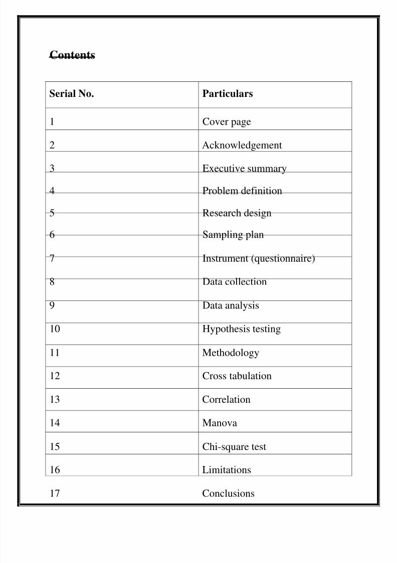
Contents

Serial No. Particulars

1 Cover page

2 Acknowledgement

3 Executive summary

4 Problem definition

5 Research design

6 Sampling plan

7 Instrument (questionnaire)

8 Data collection

9 Data analysis

10 Hypothesis testing

11 Methodology

12 Cross tabulation

13 Correlation

14 Manova

15 Chi-square test

16 Limitations

17 Conclusions



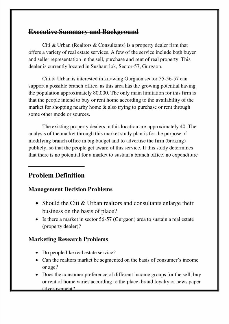
Executive Summary and Background

Citi & Urban (Realtors & Consultants) is a property dealer firm that

offers a variety of real estate services. A few of the service include both buyer

and seller representation in the sell, purchase and rent of real property. This

dealer is currently located in Sushant lok, Sector-57, Gurgaon.

Citi & Urban is interested in knowing Gurgaon sector 55-56-57 can

support a possible branch office, as this area has the growing potential having

the population approximately 80,000. The only main limitation for this firm is

that the people intend to buy or rent home according to the availability of the

market for shopping nearby home & also trying to purchase or rent through

some other mode or sources.

The existing property dealers in this location are approximately 40 .The

analysis of the market through this market study plan is for the purpose of

modifying branch office in big budget and to advertise the firm (broking)

publicly, so that the people get aware of this service. If this study determines

that there is no potential for a market to sustain a branch office, no expenditure

should be made.

Problem Definition

Management Decision Problems

Should the Citi & Urban realtors and consultants enlarge their

business on the basis of place?

Is there a market in sector 56-57 (Gurgaon) area to sustain a real estate

(property dealer)?

Marketing Research Problems

Do people like real estate service?

Can the realtors market be segmented on the basis of consumer’s income

or age?

Does the consumer preference of different income groups for the sell, buy

or rent of home varies according to the place, brand loyalty or news paperadvertisement?



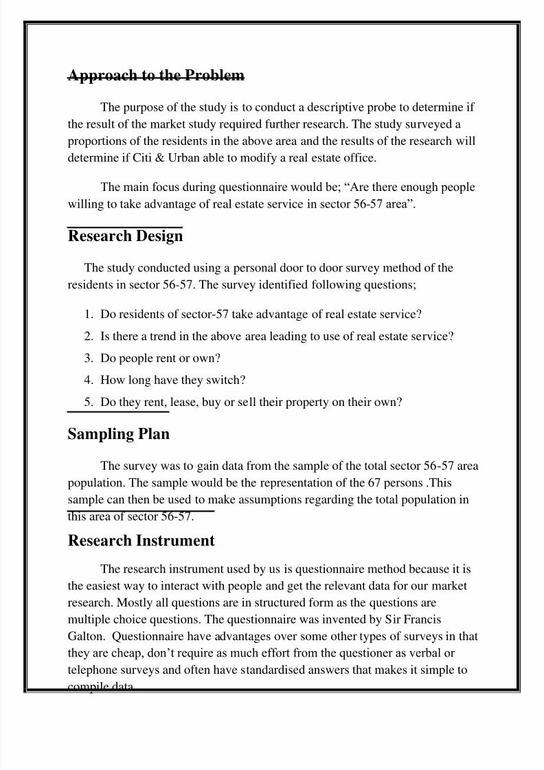
Approach to the Problem

The purpose of the study is to conduct a descriptive probe to determine if

the result of the market study required further research. The study surveyed a

proportions of the residents in the above area and the results of the research will

determine if Citi & Urban able to modify a real estate office.

The main focus during questionnaire would be; “Are there enough people

willing to take advantage of real estate service in sector 56-57 area”.

Research Design

The study conducted using a personal door to door survey method of theresidents in sector 56-57. The survey identified following questions;

1. Do residents of sector-57 take advantage of real estate service?

2. Is there a trend in the above area leading to use of real estate service?

3. Do people rent or own?

4. How long have they switch?

5. Do they rent, lease, buy or sell their property on their own?

Sampling Plan

The survey was to gain data from the sample of the total sector 56-57 area

population. The sample would be the representation of the 67 persons .This

sample can then be used to make assumptions regarding the total population in

this area of sector 56-57.

Research Instrument

The research instrument used by us is questionnaire method because it is

the easiest way to interact with people and get the relevant data for our market

research. Mostly all questions are in structured form as the questions are

multiple choice questions. The questionnaire was invented by Sir Francis

Galton. Questionnaire have advantages over some other types of surveys in that

they are cheap, don’t require as much effort from the questioner as verbal or

telephone surveys and often have standardised answers that makes it simple tocompile data.



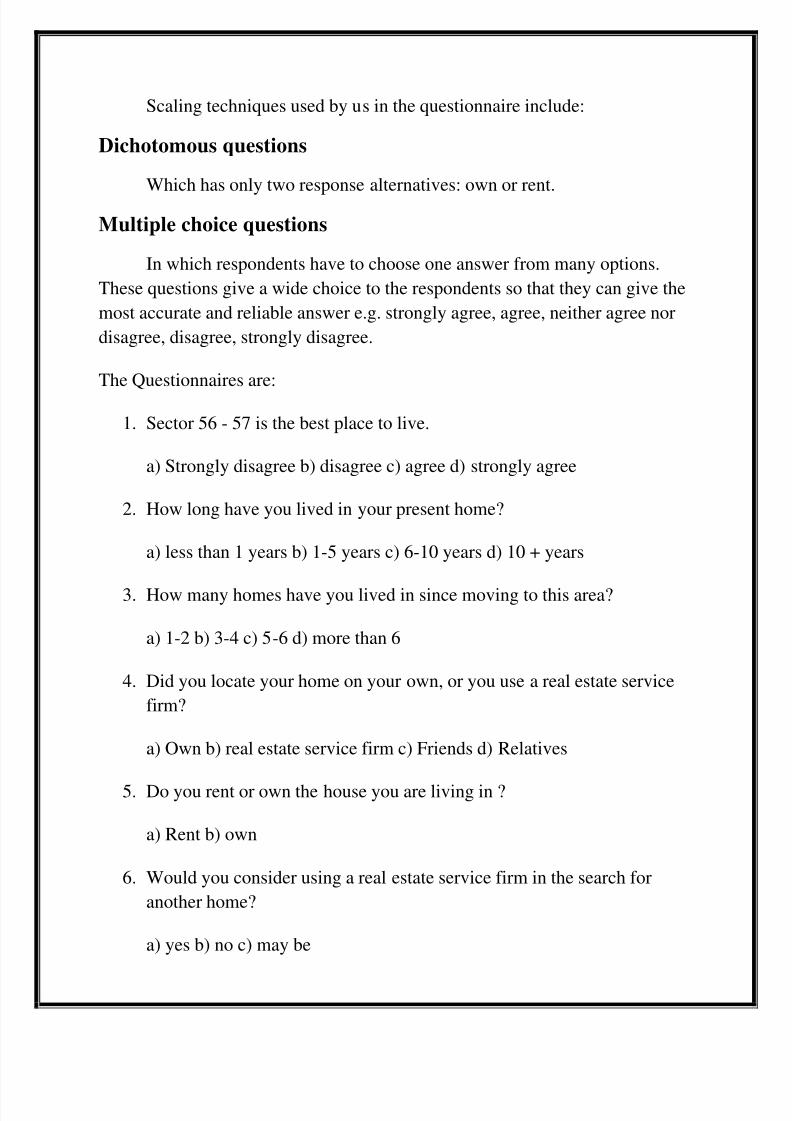
Scaling techniques used by us in the questionnaire include:

Dichotomous questions

Which has only two response alternatives: own or rent.

Multiple choice questions

In which respondents have to choose one answer from many options.

These questions give a wide choice to the respondents so that they can give the

most accurate and reliable answer e.g. strongly agree, agree, neither agree nor

disagree, disagree, strongly disagree.

The Questionnaires are:

1. Sector 56 - 57 is the best place to live.

a) Strongly disagree b) disagree c) agree d) strongly agree

2. How long have you lived in your present home?

a) less than 1 years b) 1-5 years c) 6-10 years d) 10 + years

3. How many homes have you lived in since moving to this area?

a) 1-2 b) 3-4 c) 5-6 d) more than 6

4. Did you locate your home on your own, or you use a real estate service

firm?

a) Own b) real estate service firm c) Friends d) Relatives

5. Do you rent or own the house you are living in ?

a) Rent b) own

6. Would you consider using a real estate service firm in the search for

another home?

a) yes b) no c) may be



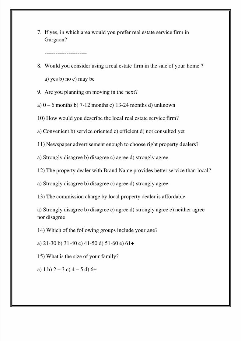
7. If yes, in which area would you prefer real estate service firm in

Gurgaon?

-----------------------

8. Would you consider using a real estate firm in the sale of your home ?

a) yes b) no c) may be

9. Are you planning on moving in the next?

a) 0 – 6 months b) 7-12 months c) 13-24 months d) unknown

10) How would you describe the local real estate service firm?

a) Convenient b) service oriented c) efficient d) not consulted yet

11) Newspaper advertisement enough to choose right property dealers?


12) The property dealer with Brand Name provides better service than local?


13) The commission charge by local property dealer is affordable

a) Strongly disagree b) disagree c) agree d) strongly agree e) neither agree

nor disagree

14) Which of the following groups include your age?

a) 21-30 b) 31-40 c) 41-50 d) 51-60 e) 61+

15) What is the size of your family?

a) 1 b) 2 – 3 c) 4 – 5 d) 6+



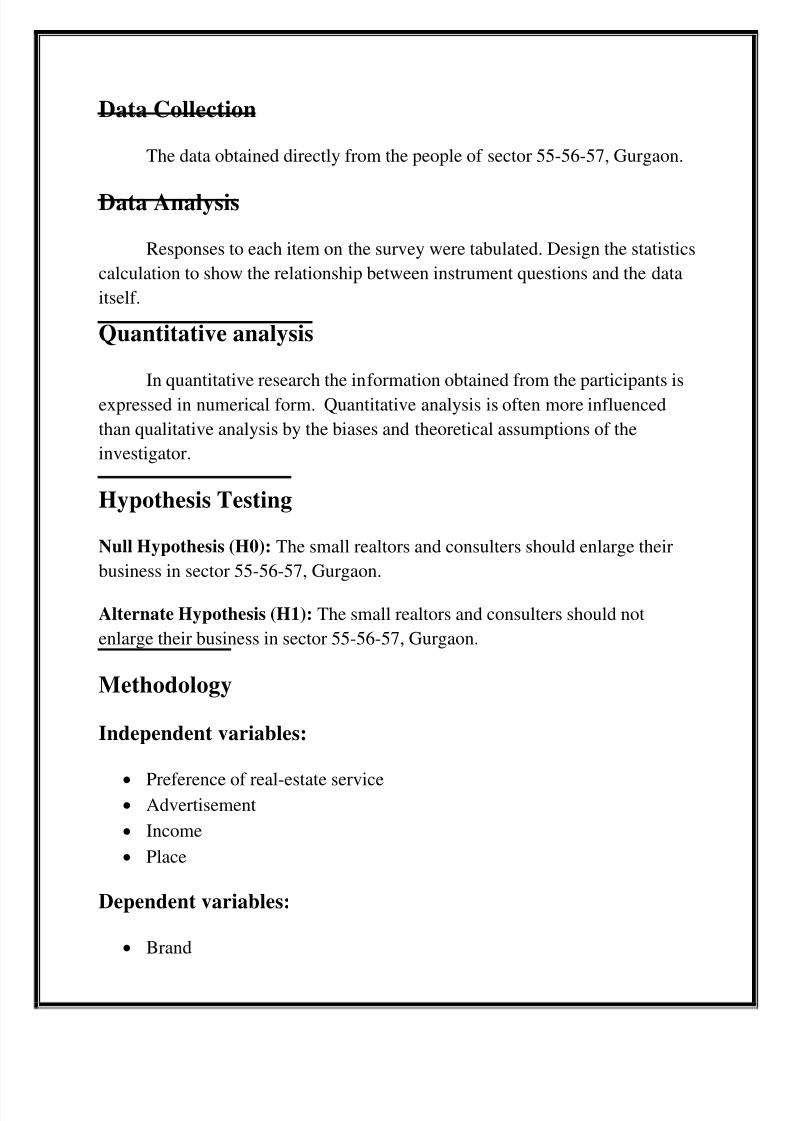
Data Collection

The data obtained directly from the people of sector 55-56-57, Gurgaon.

Data Analysis

Responses to each item on the survey were tabulated. Design the statistics

calculation to show the relationship between instrument questions and the data

itself.

Quantitative analysis

In quantitative research the information obtained from the participants is

expressed in numerical form. Quantitative analysis is often more influenced

than qualitative analysis by the biases and theoretical assumptions of the

investigator.

Hypothesis Testing

Null Hypothesis (H0): The small realtors and consulters should enlarge their

business in sector 55-56-57, Gurgaon.

Alternate Hypothesis (H1): The small realtors and consulters should not

enlarge their business in sector 55-56-57, Gurgaon.

Methodology

Independent variables:

Preference of real-estate service Advertisement

Income

Place

Dependent variables:

Brand



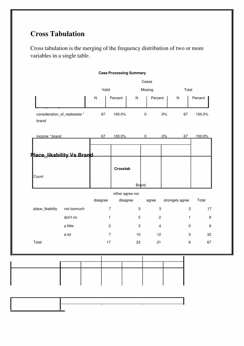
Cross Tabulation

Cross tabulation is the merging of the frequency distribution of two or more

variables in a single table.

Case Processing Summary

Cases

Valid Missing Total

N Percent N Percent N Percent

place_likability * brand 67 100.0% 0 .0% 67 100.0%

consideration_of_realestate *

brand

67 100.0% 0 .0% 67 100.0%

news_advertisement * brand 67 100.0% 0 .0% 67 100.0%

income * brand 67 100.0% 0 .0% 67 100.0%

Place_likability Vs Brand

Crosstab

Count

Brand

Totaldisagree

nither agree nor

disagree agree strongely agree

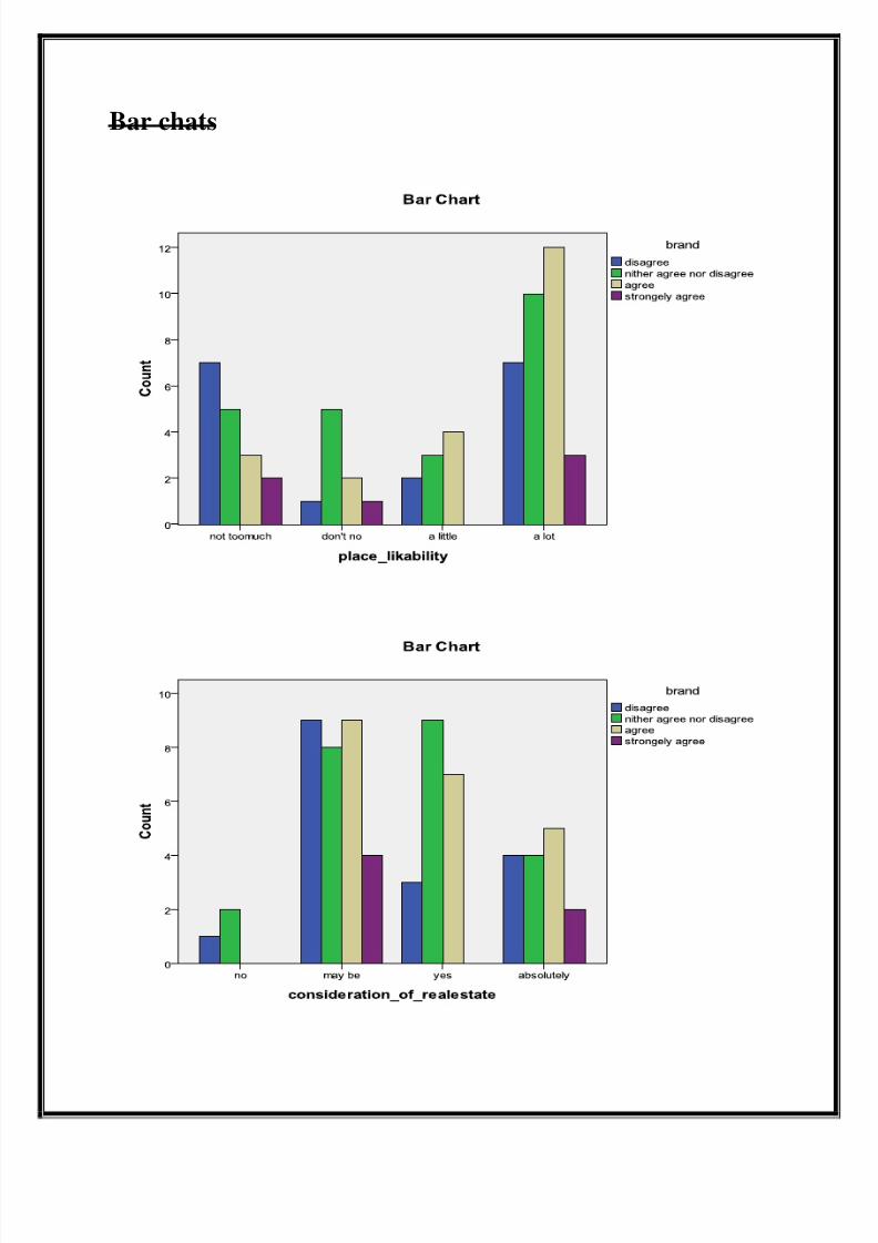
place_likability not toomuch 7 5 3 2 17

don't no 1 5 2 1 9

a little 2 3 4 0 9

a lot 7 10 12 3 32

Total 17 23 21 6 67



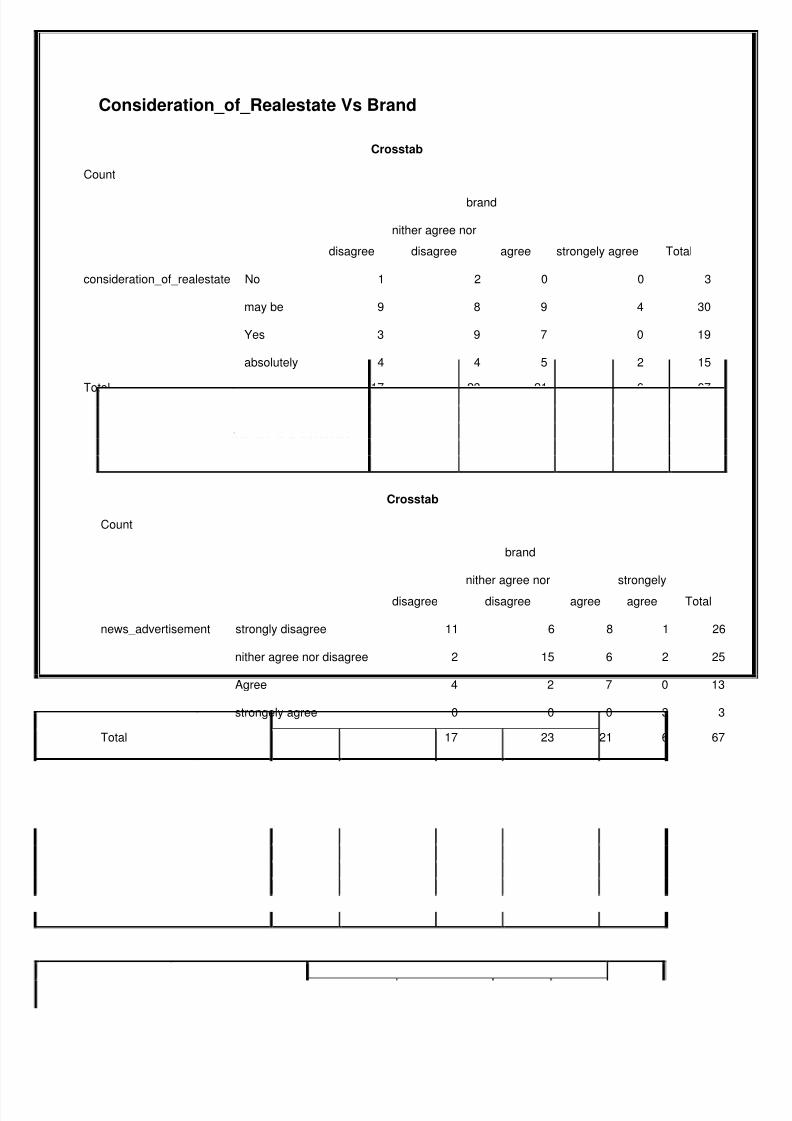
Consideration_of_Realestate Vs Brand

Crosstab

Count

brand

Totaldisagree

nither agree nor

disagree agree strongely agree

consideration_of_realestate No 1 2 0 0 3

may be 9 8 9 4 30

Yes 3 9 7 0 19

absolutely 4 4 5 2 15

Total 17 23 21 6 67

News_advertisement Vs Brand

Crosstab

Count

brand

Totaldisagree

nither agree nor

disagree agree

strongely

agree

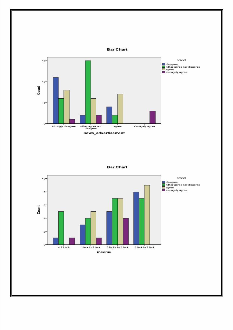
news_advertisement strongly disagree 11 6 8 1 26

nither agree nor disagree 2 15 6 2 25

Agree 4 2 7 0 13

strongely agree 0 0 0 3 3

Total 17 23 21 6 67



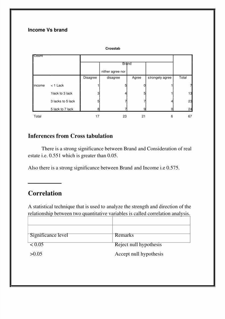
Income Vs brand

Crosstab

Count

Brand

TotalDisagree

nither agree nor

disagree Agree strongely agree

income < 1 Lack 1 5 0 1 7

1lack to 3 lack 3 4 5 1 13

3 lacks to 5 lack 5 7 7 4 23

5 lack to 7 lack 8 7 9 0 24

Total 17 23 21 6 67

Inferences from Cross tabulation

There is a strong significance between Brand and Consideration of real

estate i.e. 0.551 which is greater than 0.05.

Also there is a strong significance between Brand and Income i.e 0.575.

Correlation

A statistical technique that is used to analyze the strength and direction of the

relationship between two quantitative variables is called correlation analysis.

Significance level Remarks

< 0.05 Reject null hypothesis

>0.05 Accept null hypothesis



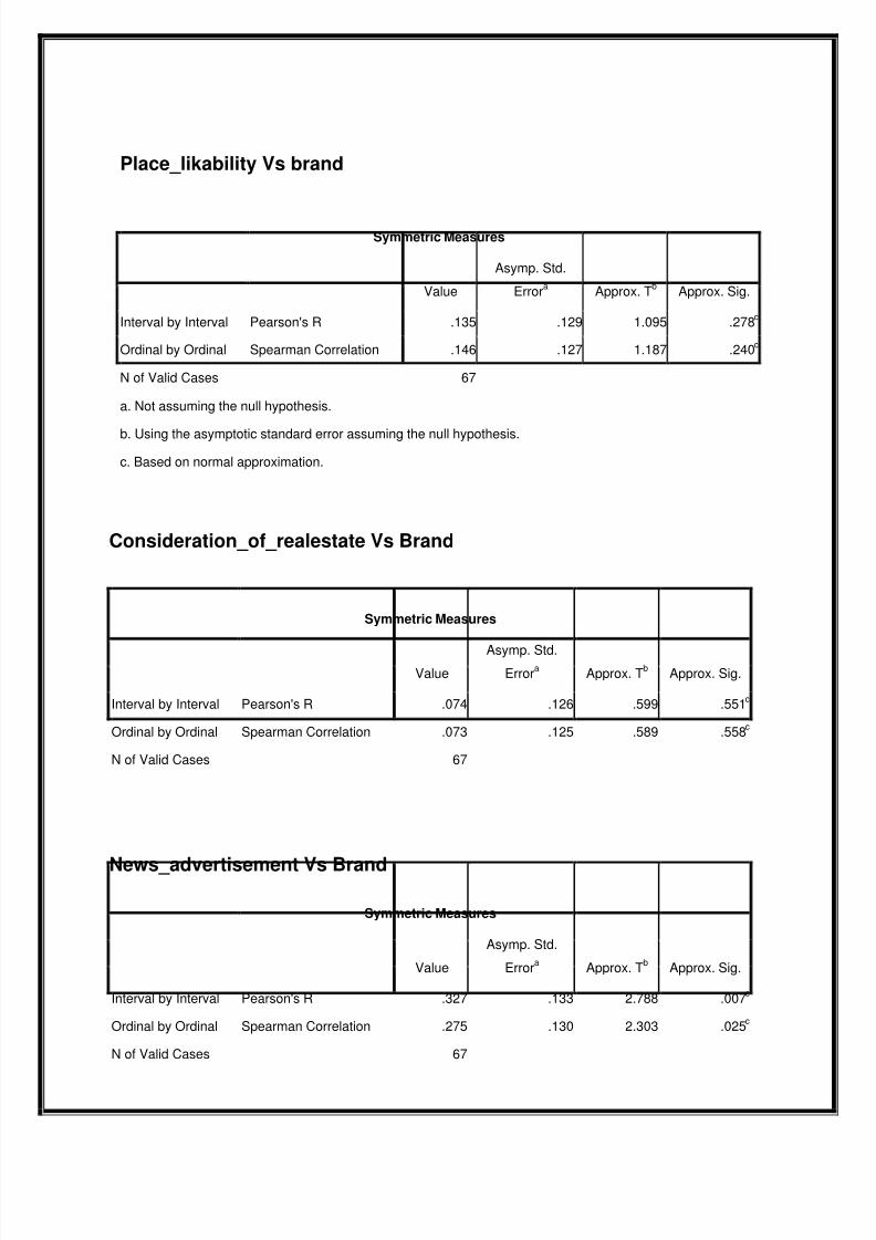
Place_likability Vs brand

Symmetric Measures

Value

Asymp. Std.

Errora

Approx. Tb

Approx. Sig.

Interval by Interval Pearson's R .135 .129 1.095 .278c

Ordinal by Ordinal Spearman Correlation .146 .127 1.187 .240c

N of Valid Cases 67

a. Not assuming the null hypothesis.

b. Using the asymptotic standard error assuming the null hypothesis.

c. Based on normal approximation.

Consideration_of_realestate Vs Brand

Symmetric Measures

Value

Asymp. Std.

Errora

Approx. Tb

Approx. Sig.

Interval by Interval Pearson's R .074 .126 .599 .551c

Ordinal by Ordinal Spearman Correlation .073 .125 .589 .558c

N of Valid Cases 67


Symmetric Measures

Value

Asymp. Std.

Errora

Approx. Tb

Approx. Sig.

Interval by Interval Pearson's R .327 .133 2.788 .007c

Ordinal by Ordinal Spearman Correlation .275 .130 2.303 .025c

N of Valid Cases 67



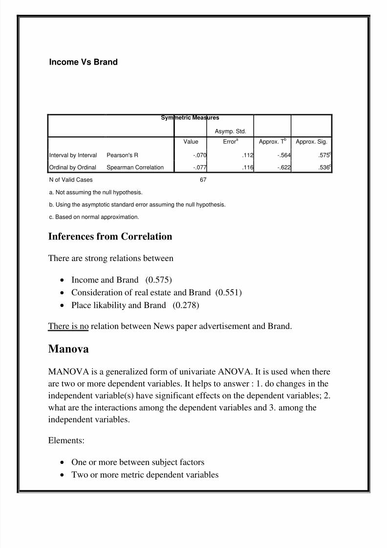
Income Vs Brand

Symmetric Measures

Value

Asymp. Std.

Errora

Approx. Tb

Approx. Sig.

Interval by Interval Pearson's R -.070 .112 -.564 .575c

Ordinal by Ordinal Spearman Correlation -.077 .116 -.622 .536c

N of Valid Cases 67

a. Not assuming the null hypothesis.

b. Using the asymptotic standard error assuming the null hypothesis.

c. Based on normal approximation.

Inferences from Correlation

There are strong relations between

Income and Brand (0.575)

Consideration of real estate and Brand (0.551)

Place likability and Brand (0.278)

There is no relation between News paper advertisement and Brand.

Manova

MANOVA is a generalized form of univariate ANOVA. It is used when there

are two or more dependent variables. It helps to answer : 1. do changes in theindependent variable(s) have significant effects on the dependent variables; 2.

what are the interactions among the dependent variables and 3. among the

independent variables.

Elements:

One or more between subject factors

Two or more metric dependent variables



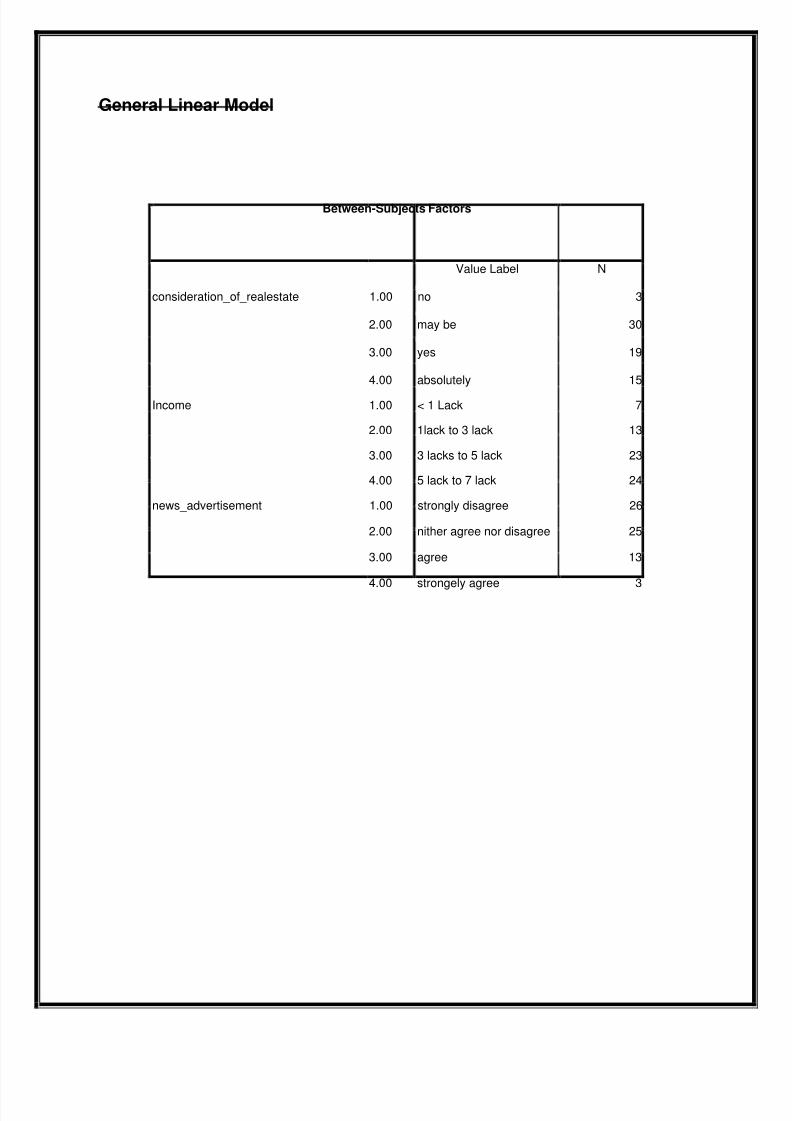
General Linear Model

Between-Subjects Factors

Value Label N

consideration_of_realestate 1.00 no 3

2.00 may be 30

3.00 yes 19

4.00 absolutely 15

Income 1.00 < 1 Lack 7

2.00 1lack to 3 lack 13

3.00 3 lacks to 5 lack 23

4.00 5 lack to 7 lack 24

news_advertisement 1.00 strongly disagree 26

2.00 nither agree nor disagree 25

3.00 agree 13

4.00 strongely agree 3



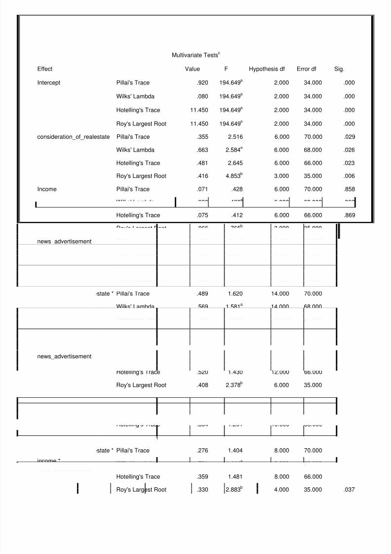
Multivariate Testsc

Effect Value F Hypothesis df Error df Sig.

Intercept Pillai's Trace .920 194.649a

2.000 34.000 .000

Wilks' Lambda .080 194.649a

2.000 34.000 .000

Hotelling's Trace 11.450 194.649a

2.000 34.000 .000

Roy's Largest Root 11.450 194.649a

2.000 34.000 .000

consideration_of_realestate Pillai's Trace .355 2.516 6.000 70.000 .029


6.000 68.000 .026

Hotelling's Trace .481 2.645 6.000 66.000 .023

Roy's Largest Root .416 4.853b

3.000 35.000 .006

Income Pillai's Trace .071 .428 6.000 70.000 .858

Wilks' Lambda .930 .420a

6.000 68.000 .863

Hotelling's Trace .075 .412 6.000 66.000 .869

Roy's Largest Root .066 .765b

3.000 35.000 .521

news_advertisement Pillai's Trace .452 3.406 6.000 70.000 .005


6.000 68.000 .005



3.000 35.000 .002


income

Pillai's Trace .489 1.620 14.000 70.000 .095


14.000 68.000 .107



7.000 35.000 .091


news_advertisement

Pillai's Trace .391 1.416 12.000 70.000 .180


12.000 68.000 .177



6.000 35.000 .049

income *

news_advertisement

Pillai's Trace .307 1.270 10.000 70.000 .264


10.000 68.000 .285



5.000 35.000 .226


income *

news_advertisement

Pillai's Trace .276 1.404 8.000 70.000 .210


8.000 68.000 .194



4.000 35.000 .037



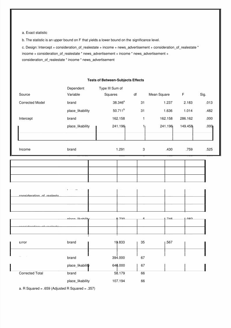
a. Exact statistic

b. The statistic is an upper bound on F that yields a lower bound on the significance level.

c. Design: Intercept + consideration_of_realestate + income + news_advertisement + consideration_of_realestate *

income + consideration_of_realestate * news_advertisement + income * news_advertisement +

consideration_of_realestate * income * news_advertisement

Tests of Between-Subjects Effects

Source

Dependent

Variable

Type III Sum of

Squares df Mean Square F Sig.

Corrected Model brand 38.346a

31 1.237 2.183 .013

place_likability 50.711b

31 1.636 1.014 .482

Intercept brand 162.158 1 162.158 286.162 .000

place_likability 241.196 1 241.196 149.458 .000

consideration_of_realestate brand 4.572 3 1.524 2.689 .061


Income brand 1.291 3 .430 .759 .525

place_likability .526 3 .175 .109 .954

news_advertisement brand 9.751 3 3.250 5.736 .003



income

brand 6.912 7 .987 1.743 .131



news_advertisement

brand 8.086 6 1.348 2.378 .049

place_likability 6.465 6 1.078 .668 .676

income * news_advertisement brand 4.137 5 .827 1.460 .228



income * news_advertisement

brand 6.530 4 1.632 2.881 .037

place_likability 1.926 4 .482 .298 .877

Error brand 19.833 35 .567

place_likability 56.483 35 1.614

Total brand 394.000 67

place_likability 646.000 67

Corrected Total brand 58.179 66


a. R Squared = .659 (Adjusted R Squared = .357)



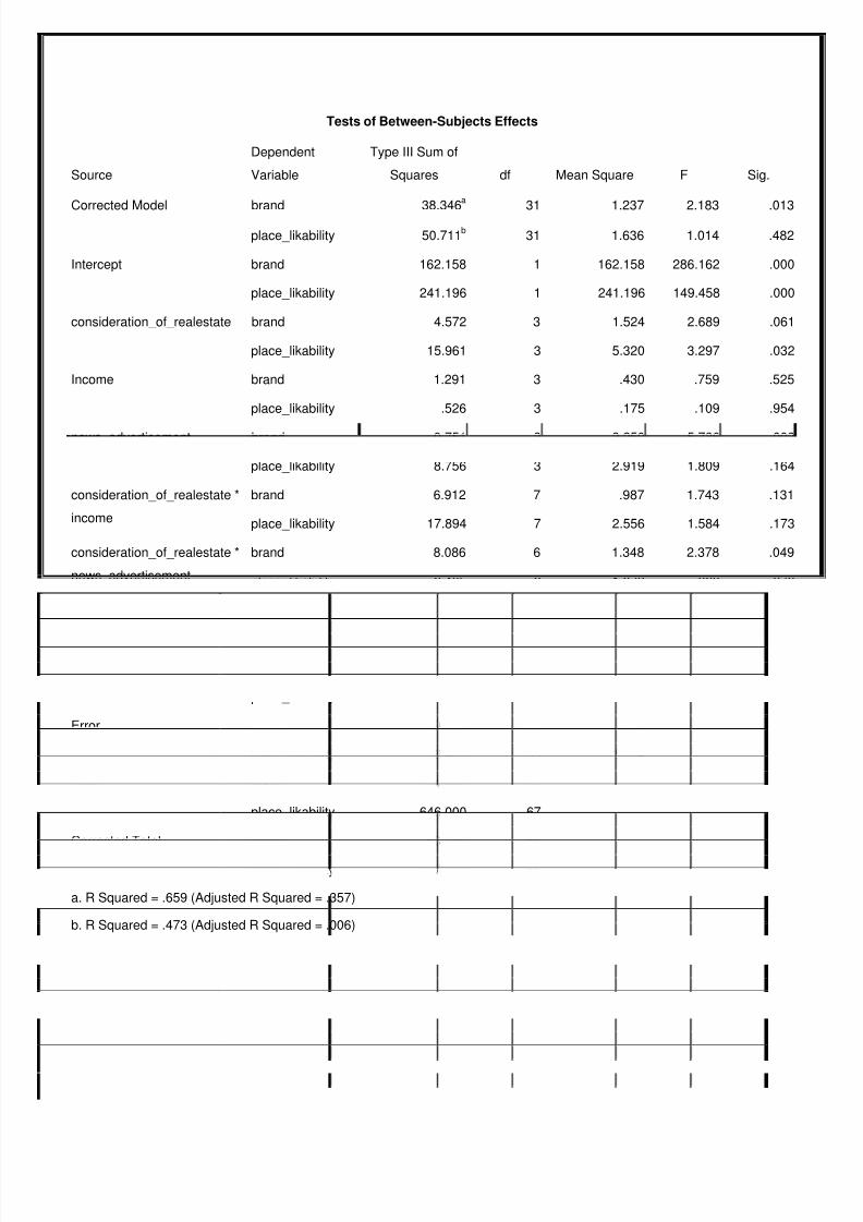
Tests of Between-Subjects Effects

Source

Dependent

Variable

Type III Sum of

Squares df Mean Square F Sig.

Corrected Model brand 38.346a

31 1.237 2.183 .013

place_likability 50.711b

31 1.636 1.014 .482

Intercept brand 162.158 1 162.158 286.162 .000


consideration_of_realestate brand 4.572 3 1.524 2.689 .061


Income brand 1.291 3 .430 .759 .525

place_likability .526 3 .175 .109 .954

news_advertisement brand 9.751 3 3.250 5.736 .003



income

brand 6.912 7 .987 1.743 .131



news_advertisement

brand 8.086 6 1.348 2.378 .049

place_likability 6.465 6 1.078 .668 .676

income * news_advertisement brand 4.137 5 .827 1.460 .228



income * news_advertisement

brand 6.530 4 1.632 2.881 .037

place_likability 1.926 4 .482 .298 .877

Error brand 19.833 35 .567

place_likability 56.483 35 1.614

Total brand 394.000 67


Corrected Total brand 58.179 66


a. R Squared = .659 (Adjusted R Squared = .357)

b. R Squared = .473 (Adjusted R Squared = .006)



Bar chats





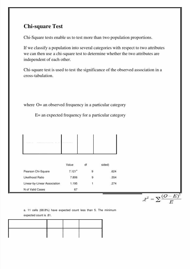
Chi-square Test

Chi-Square tests enable us to test more than two population proportions.

If we classify a population into several categories with respect to two attributeswe can then use a chi-square test to determine whether the two attributes are

independent of each other.

Chi-square test is used to test the significance of the observed association in a

cross-tabulation.

where O= an observed frequency in a particular category

E= an expected frequency for a particular category

Place_likability Vs Brand

Chi-Square Tests

Value df

Asymp. Sig. (2-

sided)

Pearson Chi-Square 7.121a

9 .624

Likelihood Ratio 7.806 9 .554

Linear-by-Linear Association 1.195 1 .274

N of Valid Cases 67

a. 11 cells (68.8%) have expected count less than 5. The minimum

expected count is .81.



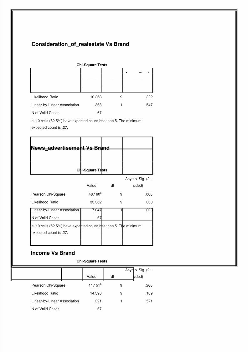
Consideration_of_realestate Vs Brand

Chi-Square Tests

Value df

Asymp. Sig. (2-

sided)


9 .560


Linear-by-Linear Association .363 1 .547

N of Valid Cases 67




Chi-Square Tests

Value df

Asymp. Sig. (2-

sided)


9 .000


Linear-by-Linear Association 7.047 1 .008

N of Valid Cases 67



Income Vs Brand

Chi-Square Tests

Value df

Asymp. Sig. (2-

sided)


9 .266


Linear-by-Linear Association .321 1 .571

N of Valid Cases 67



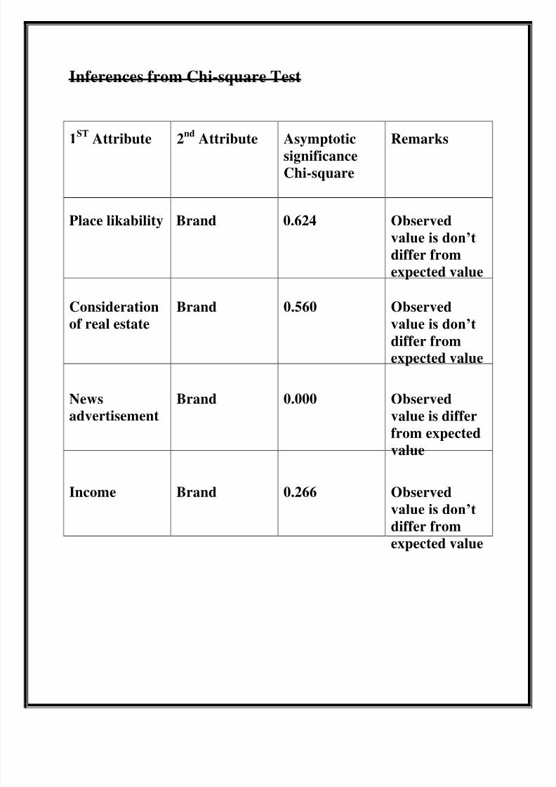
Inferences from Chi-square Test

1ST Attribute 2nd Attribute Asymptoticsignificance

Chi-square

Remarks

Place likability Brand 0.624 Observed

value is don’t

differ from

expected value

Consideration

of real estate

Brand 0.560 Observed

value is don’t

differ from

expected value

News

advertisement

Brand 0.000 Observed

value is differfrom expected

value

Income Brand 0.266 Observed

value is don’t

differ from

expected value



Study Limitations

This includes Respondent Errors

There are two types of respondent errors. They are, Non-Response Error

and Response Error. Non- Response errors include non-respondents error,

where people could refuse to cooperate. Here people could refuse to answer

some questions like information relating to the amount of income they receive

per month or their age.

Customers could also answer questions with a certain incline that does

not represent the truth completely. This is called a response bias. Here theanswers are misinterpreted or falsified.

The interviewer could sometimes influence the way the respondent

answers the question. The presence of the interviewer could make the

respondent modify their answer so that the interviewer does not see them as un-

usual.

Social desirability bias is also a form of response bias. This is when

people try to create a good impression in the interviewer’s presence. A good

example can be when respondents are answering a question about the amount of

income they earn per month. The respondents may give an answer of a higher

income than what they truly receive, especially if they are planning on going to

a better paying job in a few months or years to come.

Administrative Errors:

This refers to errors caused by “the improper administration or executionof the research task” by the researchers.

Data Processing Error:

This is when the researcher codes the data received from the interview or

questioner wrongly on the computer. E.g., a researcher can code the age of a

respondent wrongly on the computer, and this might affect the end result of the

survey conducted.



Interviewer Error:

This can occur when the interviewer incorrectly records the responses

from the survey.

Interviewer Cheating: This is when the interviewer fills in questions that were left out by the

respondent.

Conclusion

Null hypothesis is accepted because:

There are strong relations between:

Income and Brand (0.575)

Consideration of real estate and Brand (0.551)

Place likability and Brand (0.278)

Also from the chi-square test it is clear that the p value is greater in maximum

cases it means that observed values do not differ significantly from expectedvalue.

The realtors and consultants should enlarge their businesses in sector 55-56-57

(Gurgaon), by spending more money. So that it will be beneficial for them.

Documents

BADM Project Report Group-10